Name :

Homework Project #5Math 365, Fall 2015

Due November 6th

You may work in terms of two on this homework assignment.

1. (Splines) For this problem, you will use the Matlab routine spline to create a spline interpolant forthe two data sets dq1.dat and dq2.dat from the course website.

(a) Use the the Matlab function spline to create a spline interpolant for the two curves describedby the data sets. Plot the results of your data interpolant.

Here are a few tips.

• You will want to add the command

set(gca,’ydir’,’reverse’);

after your plot command so that your image is oriented correctly!

• Be sure to plot your final spline using enough data points. I suggest evaluating your resultingspline at roughly 2000 data points.

• Write a function which loads a file name, extracts the data, does the spline interpolation, andplots the results. Then call this function for each of the two data files.

• Note : It is not enough to just plot a the data points and connect them with linearinterpolants! You must fit a spline through the data points.

(b) (5 points Extra credit) What famous artist created this drawing?

2. (Piecewise Cubic Hermite Interpolating Polynomial) The Matlab function pchip is a piecewisepolynomial that has the feature that its values do not produce values larger than those that appearin the data. This is particularly useful for data that should physically remain within a given interval.In this problem, you will use pchip to interpolate measurements of fractional water content measuredfrom various depths in a snowpack. The data file, snow.dat, is available on the course website. Thefirst column of this file is a measurement of snow depth (cm), and second column is the percentageof liquid water content p, 0 < p < 100 found at that depth. Plot your interpolating polynomial andinclude the following

• Include your data points in your plot (use markersize).

• Plot the snow depth on the y-axis so that zero depth is at the top of the plot, and 200 cm is atthe bottom. Hint: Use set(gca,’ydir’,’reverse’).

• Plot the water content along the x-axis.

• Add a title and axis labels.

• Use your interpolation routine to approximate the snow water content at a depth of 106.3 cen-timeters. Write your results to the file watercontent.out (using write file).

• Why is this particular choice of derivatives particularly advantageous for this data set?

(Thanks to Santiago Rodriguez, Department of Geophysics (BSU) and former Math 365 student, forthe snow data.)

1

3. (Roller Coaster!) For this problem, you will use the spline function to construct a closed-loop rollercoaster track. On this track, you’ll plot vectors indicating the strength of the centrifugal force as yougo around the track.

To construct the track, download the file rollercoaster.dat. This file contains a list of points,(t, x(t), y(t), z(t)) for the parameterized curve describing the track.

Then do the following.

(a) Plot a closed curve through these points using the spline function and the plot3 function. Thiscurve should resemble a roller-coaster.

(b) Assume that the cars on this roller coaster are attached to a cable on the tracks, and this cablepulls the cars around the roller coaster track at constant speed S = 60. Also, assume that the carsare always oriented outwards in the direction of the normal to the curve. Sitting in the car, youwon’t experience any acceleration in the direction tangent to the tracks, but you will experiencecentrifugal force as you bend around the curves. This acceleration can be described as

a(α) = S2κ(α)N(α)

where α is the parameter you have used to model the spline, κ(α) is the curvature of the track,and N(α) is a vector perpendicular to the direction of travel.

Plot acceleration vectors on your roller coaster at several points on the ride. The plot in Figure 1shows 50 vectors per polynomial segment. These vectors illustrate how the acceleration is largerin regions with tight curvature. Use the cubic spline you found, and notes on the course websiteto compute the normal N(α) and the curvature κ(α). Scale your acceleration vectors by gravityg = 9.81 so they plot nicely.

(c) (Extra credit - 5 points) You will notice that your acceleration vectors are not continuous atthe point where the first and last data point meet. Figure out a way to get at least continuousfirst and second derivatives at this point. Hint: One way to do this is to use the function csape

from the curve-fitting toolbox. This function gives you many more options for end-conditions(including the periodic end point conditions) than does the spline function. A second way todo this is to implement the cubic spline, along with periodic boundary conditions as discussed onthe online notes.

For this problem, you will need the functions spline, norm, polyder, polyval, cross, mkpp and ppval.

For hints on how to do this problem, see the tutorial on the course website on “Splines and the geometryof curves”. See Figure 1 for an example of what your final plot should look like.

4. (Newton’s method) The almost universally used algorithm to compute√a, where a > 0, is the

recursion

xn+1 =1

2

(xn +

a

xn

), (1)

easily obtained by means of Newton’s method for the function f(x) = x2 − a. One potential problemwith this method is that it requires a floating point division, which not all computer processors support,or which may too expensive for a particular application.

For these reasons, it is advantageous to devise a method for computing the square root that does notrequire any floating point divisions, (except division by 2, which can be easily done by shifting thebinary representation one bit to the right), but only addition, subtraction and multiplication. Thetrick for doing this is to use Newton’s method to compute 1√

a, and then obtain

√a by multiplying by

a.

Your goal is to write an algorithm for computing the square root using this trick above. Division by 2is allowed, but no other floating point division. Your algorithm should work for any input value a > 0.

2

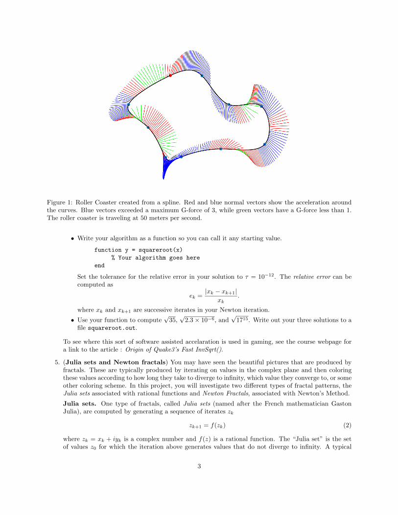
Figure 1: Roller Coaster created from a spline. Red and blue normal vectors show the acceleration aroundthe curves. Blue vectors exceeded a maximum G-force of 3, while green vectors have a G-force less than 1.The roller coaster is traveling at 50 meters per second.

• Write your algorithm as a function so you can call it any starting value.

function y = squareroot(x)

% Your algorithm goes here

end

Set the tolerance for the relative error in your solution to τ = 10−12. The relative error can becomputed as

ek =|xk − xk+1|

xk.

where xk and xk+1 are successive iterates in your Newton iteration.

• Use your function to compute√

35,√

2.3× 10−6, and√

1715. Write out your three solutions to afile squareroot.out.

To see where this sort of software assisted accelaration is used in gaming, see the course webpage fora link to the article : Origin of Quake3’s Fast InvSqrt().

5. (Julia sets and Newton fractals) You may have seen the beautiful pictures that are produced byfractals. These are typically produced by iterating on values in the complex plane and then coloringthese values according to how long they take to diverge to infinity, which value they converge to, or someother coloring scheme. In this project, you will investigate two different types of fractal patterns, theJulia sets associated with rational functions and Newton Fractals, associated with Newton’s Method.

Julia sets. One type of fractals, called Julia sets (named after the French mathematician GastonJulia), are computed by generating a sequence of iterates zk

zk+1 = f(zk) (2)

where zk = xk + iyk is a complex number and f(z) is a rational function. The “Julia set” is the setof values z0 for which the iteration above generates values that do not diverge to infinity. A typical

3

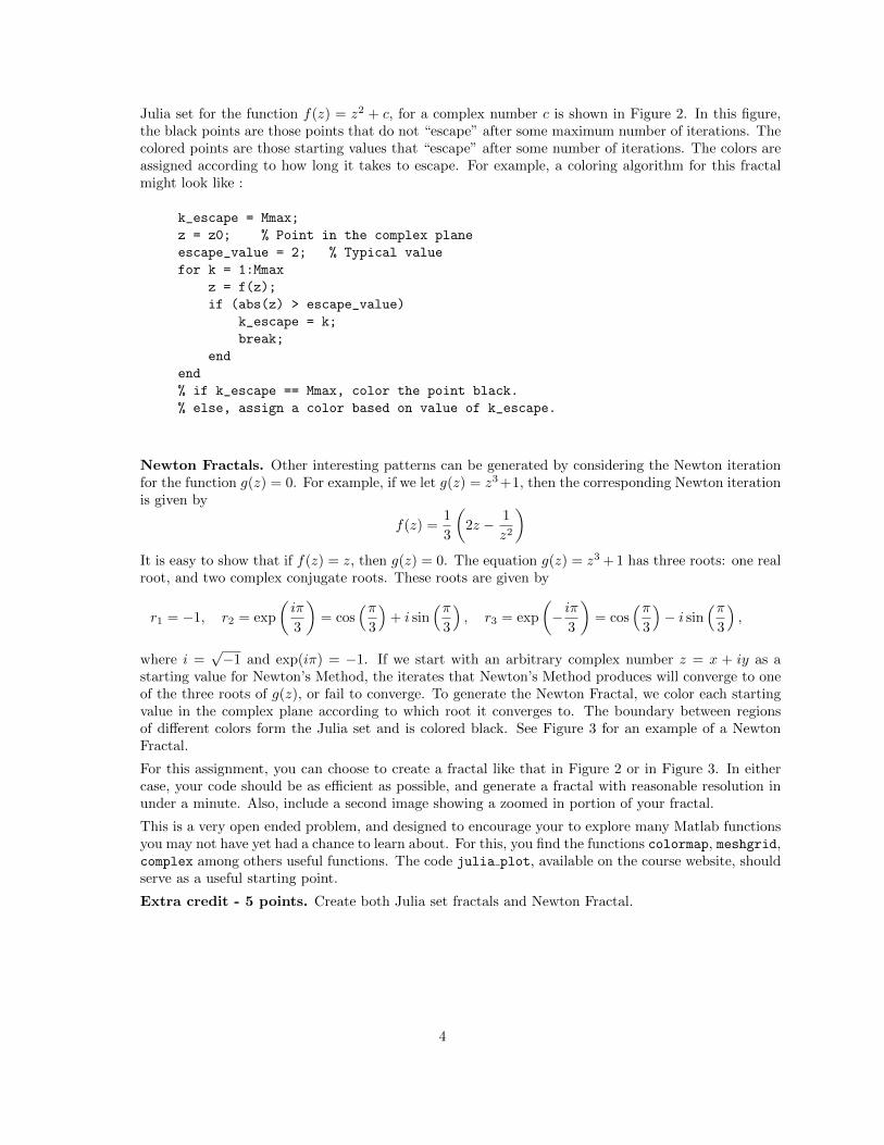
Julia set for the function f(z) = z2 + c, for a complex number c is shown in Figure 2. In this figure,the black points are those points that do not “escape” after some maximum number of iterations. Thecolored points are those starting values that “escape” after some number of iterations. The colors areassigned according to how long it takes to escape. For example, a coloring algorithm for this fractalmight look like :

k_escape = Mmax;

z = z0; % Point in the complex plane

escape_value = 2; % Typical value

for k = 1:Mmax

z = f(z);

if (abs(z) > escape_value)

k_escape = k;

break;

end

end

% if k_escape == Mmax, color the point black.

% else, assign a color based on value of k_escape.

Newton Fractals. Other interesting patterns can be generated by considering the Newton iterationfor the function g(z) = 0. For example, if we let g(z) = z3+1, then the corresponding Newton iterationis given by

f(z) =1

3

(2z − 1

z2

)It is easy to show that if f(z) = z, then g(z) = 0. The equation g(z) = z3 + 1 has three roots: one realroot, and two complex conjugate roots. These roots are given by

r1 = −1, r2 = exp

(iπ

3

)= cos

(π3

)+ i sin

(π3

), r3 = exp

(− iπ

3

)= cos

(π3

)− i sin

(π3

),

where i =√−1 and exp(iπ) = −1. If we start with an arbitrary complex number z = x + iy as a

starting value for Newton’s Method, the iterates that Newton’s Method produces will converge to oneof the three roots of g(z), or fail to converge. To generate the Newton Fractal, we color each startingvalue in the complex plane according to which root it converges to. The boundary between regionsof different colors form the Julia set and is colored black. See Figure 3 for an example of a NewtonFractal.

For this assignment, you can choose to create a fractal like that in Figure 2 or in Figure 3. In eithercase, your code should be as efficient as possible, and generate a fractal with reasonable resolution inunder a minute. Also, include a second image showing a zoomed in portion of your fractal.

This is a very open ended problem, and designed to encourage your to explore many Matlab functionsyou may not have yet had a chance to learn about. For this, you find the functions colormap, meshgrid,complex among others useful functions. The code julia plot, available on the course website, shouldserve as a useful starting point.

Extra credit - 5 points. Create both Julia set fractals and Newton Fractal.

4

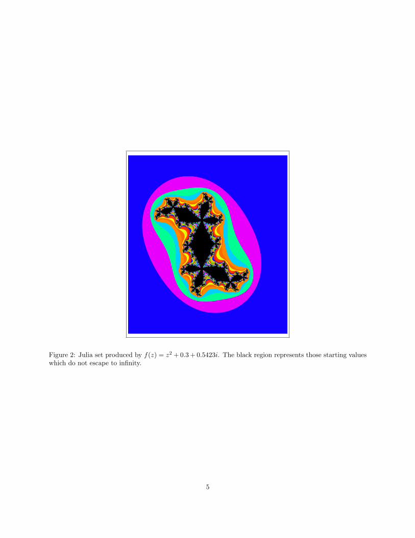
Figure 2: Julia set produced by f(z) = z2 + 0.3 + 0.5423i. The black region represents those starting valueswhich do not escape to infinity.

5

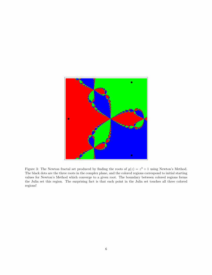
Figure 3: The Newton fractal set produced by finding the roots of g(z) = z3 + 1 using Newton’s Method.The black dots are the three roots in the complex plane, and the colored regions correspond to initial startingvalues for Newton’s Method which converge to a given root. The boundary between colored regions formsthe Julia set this region. The surprising fact is that each point in the Julia set touches all three coloredregions!

6