Embed Size (px)
Citation preview

MATH 53 NOTES
ARUN DEBRAYMARCH 2, 2014
These notes were taken in Stanford’s Math 53 (Ordinary Differential Equations) class in Spring 2013, taught by Akshay Venkatesh.I live-TEXed them using vim, and as such there may be typos; please send questions, comments, complaints, and corrections [email protected].
Contents
1. Overview: 4/1/13 12. First-Order Linear Differential Equations: 4/3/13 23. Examples of Integrating Factors: 4/5/13 44. Separation of Variables: 4/8/13 55. Autonomous Equations: 4/10/13 76. Exact Equations: 4/12/13 97. More Exact Equations: 4/15/13 108. Numerical Methods and Existence and Uniqueness: 4/17/13 119. Review of Weeks 1 to 3: 4/19/13 1210. Systems of Differential Equation: 4/22/13 1311. Review of Linear Algebra: 4/24/13 1512. Systems of Linear Equations: 4/26/13 1613. Complex Eigenvalues: 4/29/13 1714. Complex Exponentials: 5/1/13 1815. Repeated Eigenvalues: 5/6/13 1916. Variation of Parameters I: 5/8/13 2017. Variation of Parameters II: 5/10/13 2118. Review of Weeks 4 to 6: 5/13/13 2219. Second Order Linear Systems: 5/15/13 2320. Inhomogeneous Second-Order Equations: 5/17/13 2421. The Laplace Transform: 5/20/13 25
Note that I never took Math 53, but that I audited classes in order to understand the material better. Beware of typos.
1. Overview: 4/1/13
A little bit of administrative stuff: homework will be due Thursdays, and here is the course website.Let’s start with an example:
Theorem 1.1. Suppose the population of the United States is 315 million, and grows by 0.75% each year. Let P(t)be the population in year t, so that P(2012) = 315. Then, P(t + 1) = P(t) + 0.0075P(t). But the population growscontinuously, so consider the derivative: P′(t) = 0.0075P(t).
This is a simple differential equation, which is an equation relating a function f (x) and its derivatives d fdx , d2 f
dx2 etc.,and the goal is to find f . This course will develop techniques for solving standard classes of ODEs.
1
Example 1.1. Another example is a pendulum swinging on a rod. Let θ be the angle of the rod with the vertical, sothat the pendulum satisfies the equation
d2θ
dt2 +g`
sin θ = 0,
where g is the acceleration due to gravity. This equation comes from the equation F = ma: F = −mg sin θ and a = ` d2θdt2 .
This equation is already not so simple to solve, since the sine is a tricky function. The exact solution will be givenin terms of an integral rather than familiar elementary functions. However, if θ is small, then one can approximatesin θ ≈ θ, giving the approximate differential equation d2θ
dt2 + gθ/` = 0. This is much simpler to solve.
Differential equations often model how systems change with time1
Example 1.2. Planetary motion is also given by a differential equation: again using F = ma, suppose the sun islocated at the origin in the plane. Then, the system becomes
d2xdt2 = −C
x
(x2 + y2)32
d2ydt2 = −C
y
(x2 + y2)32
,
where C depends on the masses of the sun and the planet and the gravitational constant. This is a system of twodifferential equations, which looks trickier but isn’t all that much worse.
This example is somewhat complicated, because the functions themselves are, and will resurface near the end of thecourse.
Other examples include calculating airflow or weather. Some of these involve partial differential equations (e.g.differentiating with respect to time and space), which are beyond the scope of this course. Many of these are toocomplicated to solve analytically, and instead numerical approximations are sought.
Differential equations can be classified by their order: for example, a first-order differential equation involves onlythe first derivative of a function. Example 1.1 is first-order, but the others given above aren’t.
Differential equations can also be linear: the function y and its derivatives occur only as multiplied by a function ofx. For example, y′ + y = 3 and xy′ + x2y = sin x are both linear, but y′ + sin y = y2 and the equation in Example 1.1aren’t. Linear equations are easier to solve, but many important equations are nonlinear.
Thus, the simplest differential equations are first-order and linear. These look like A(x)y′ + B(x)y = C(x).2 Anylinear first-order equation can be rewritten by dividing by A:
dydx
+B(x)A(x)︸︷︷︸b(x)
y =C(x)A(x)︸︷︷︸c(x)
.
Simplifying even further, suppse c(x) and b(x) are constants: y′ = c − by. These are the simplest differential equations.Solving this requires a trick (as do differential equations in general; sadly, these tricks are somewhat hard to motivate
most of the time). Dividing by c − by, one has1
c − bydydx
= 1
=⇒ddx
(log(c − by)−b
)= 1 (just using the Chain Rule)
Let A be a constant of integration. Then, after integrating,
=⇒ −log(c − by)
b= x + A
=⇒ c − by = e−bxe−bA
=⇒ y =cb− e−bx
(e−bA
b
).
Then, e−bA/b is some arbitrary constant, so call it K. Thus, the solution to the differential equation is y = c/b − Ke−bx.This is the general solution to y′ = c − by; K is an arbitrary constant, but given y(0) (or y at any other value of x) it ispossible to determine k.
1. . . as well as changes in space, though that won’t be discussed today.2There are plenty of first-order equations that aren’t linear at all, such as yeyy′ + x3 = 0.
2

For example, if y′ = 1 − y and y(0) = 2, then b = c = 1, so y = 1 − Ke−x for some K. Then, 2 = 1 − Ke0, so K = 1,and the specific solution is y = 1 + e−x.
2. First-Order Linear Differential Equations: 4/3/13
Last time, we considered first-order linear differential equations with constant coefficients, such as y′ = 1 + y. Whensolving, a solution was obtained by finding something which had a specified function as its derivative. This can also bethought of as multiplying by dx:
11 + y
dydx
= 1
=⇒dy
1 + y= dx
=⇒
∫dy
1 + y=
∫dx
log(1 + y) = x + C
and then the equation can be solved as before. This is called separation of variables, and will resurface next week.One can produce plots of integral curves: if the solution depends on a parameter K, it is possible to plot several
curves to get an idea of the family of solutions; see Figure 1.
Figure 1. Integral curves of y′ = 1 + y, with y(0) ∈ {−10, . . . , 10}.
In fact, this can be done without a solution, plotting direction fields, and obtaining a numerical solution. See Sections1.1 and 1.3 of the book for more details. If y(0) = 2 and y′ = 1 + y, then near 0 y′ ≈ −1, so y(0.1) ≈ y(0) − 0.1 = 1.9.This approximation is only good near zero. After successive approximations, one discovers that y(1) ≈ 1.349. Using theexact solution, y(1) = 1.366, so this can be pretty useful. This method works for any first-order differential equation,linear or not.
Some applications of differential equations: population growth modeling was discussed in the previous lecture,though it can often be more nuanced: there can be many sources of population growth or loss, and they may be given bytheir own equations. Alternatively, one can consider the cooling of a hot object, or the concentration of (for example) adrug in someone’s bloodstream. These should help with intuition for the constants given in the solutions; they providesome specific physical constant that gives the particular solution from the general formula.
Now, it is possible to generalize: consider only first-order linear differential equations, but with possibly nonconstantcoefficients, such as xy′+x2y = sin x or exy′+xy = 1/(1+x). Any such equation can be put into the form y′+p(x)y = q(x)by dividing by the y′-coefficient: the first example above becomes y′ + xy = sin x
x . Here, p(x) can represent some growth3
or removal rate, and q(x) measures the amount that is externally added or removed. Of course, there are cases in whichthey might represent something different, but this representation aids intuition.
To motivate the general case, y′ = 1 − y will be solved in a somewhat different way: rewrite it as y′ + y = 1 andmultiply it by something such that the left hand side looks like a derivative: M(x)y′ + M(x)y = M(x). It would be niceif we had My′ + M′y, so we need M to be its own derivative. Take M = ex:
exy′ + exy = ex
=⇒ddx
(exy) = ex
=⇒ exy = ex + C
y = 1 + Ce−x.
Example 2.1. Another example, this one slightly more complicated. Suppose y + y′ = e−x. Then, multiplying by ex,exy′ + exy = 1, so exy = x + C, or y = xe−x + Ce−x.
Now, let’s take the general case for a first-order linear differential equation y′ + p(x)y = q(x). Again, we will multiplyby the integrating factor M(x), in order to make the equation easier to integrate. Take M = e
∫p(x) dx (which will be
motivated later; right now, it just works, since you obtain the right derivative), and take
M(x)q(x) = M(x)dydx
+ M(x)p(x)y
=ddx
(M(x)y)
=⇒ M(x)y =
∫M(x)q(x) dx
=⇒ y =
∫M(x)q(x) dx
M(x).
A closed-form solution depends on being able to find∫
M(x)q(x), but it’s an explicit solution in either case.
Example 2.2. In y′ + y/x = sin x, p(x) = 1/x, so M(x) = elog x = x. Thus, the formula is
y =
∫x sin x dx
x=−x cos x + sin x
x+ C = − cos x +
sin xx
+ C.
after integration by parts.
3. Examples of Integrating Factors: 4/5/13
Integrating factors as discussed in the last lecture seem like magic, but in solving an equation y′ + p(x)y = q(x), onechooses M(x) = e
∫p(x) dx, so that by the Chain Rule dM
dx = p(x)M(x). Thus, the differential equation can be multipliedby M(x) to obtain y′M + yM′ = qM, so the solution is y =
(∫q(x)M(x) dx
)/M(x).
Example 3.1. Consider a bank account with variable interest. let M(t) be the amount of money in the account at timet, measured in years (though the specific unit isn’t important conceptually), and let I(t) be the rate of interest at time t:for example, 3% interest corresponds to I(t) = 0.03. Finally, let Q(t) be the amount of money put in (or negative forremoving money) in year t. Thus, M(t) obeys the differential equation
dMdt
= I(t)M(t) + Q(t).
This illustrates a common trend: the first term indicates how it would grow independent of external forces, and thesecond term represents external influences.
This can be solved in different ways: first, suppose Q(t) = 0 and I(t) = I is constant. Then, M(t) = M(0)eIt, as hasbeen done in calculus classes. If I(t) can vary, then M(t) = M(0)e
∫ t0 I(u) du, where the integral represents the average
value of the interest rate.When Q(t) isn’t zero, it can be broken into the cases Q(0),Q(1), . . . , giving a solution
M(t) = M(0)e∫ t
0 I(u) du + Q(1)e∫ t
1 I(u) du + Q(2)e∫ t
2 I(u) du + . . .4
This is an approximation assuming money is only added once at the end of each year. If it is done continuously, the sumshould be replaced by an integral:
M(t) = M(0)e∫ t
0 I(u) du +
∫ t
0Q(x)e
∫ tx I(u) du dx.
This could have also been derived with the method of integrating factors, or more specifically, the given general solutionfor first-order linear equations. The M(0)-term comes from the constant of integration, so a little bit of algebra isinvolved.Example 3.2. Consider the equation y′ = sin(t) − y. This approximates a common phenomenon: it models thetemerature of an object that’s being alternately heated and cooled (for example, a body of water heated in the day andcooled at night, or some sort of yearly temperature variation). Without the sine term, y′ = −y is Newton’s Law ofCooling, but adding it in gives a reasonably crude model. To solve, rewrite it as y′ + y = sin t and multiply by M(t) = et.Thus,
ety′ + ety = et sin t
=⇒ y =
∫et sin t dt
et .
This is an integration by parts: ∫et sin t dt = et sin t −
∫et cos t dt
= et sin t − et cos t −∫
et sin t dt
=⇒ 2∫
et sin t dt = et sin t − et cos t
=⇒
∫et sin t dt =
et sin t − et cos t2
+ C.
Plugging this back into the differential equation,
y =sin t − cos t
2+ Ce−t.
The second term is not very large, particularly as t becomes large. However, sin t − cos t =√
2 sin (t − π/4), so thetemperature oscillates with the heating and cooling, but it las behind by 1/8 of a full heating-cooling cycle. Of course,this is an approximation, but it still says interesting things: a more realistic model is y′ = sin t− ay, where a is a constantrepresenting how quickly the object cools or heats. Then, the lag depends on a: it becomes lesser as a increases.Exercise 3.1. Solve the refined model y′ = sin t − ay, and determine how the lag depends on a.
Moving to the next topic, we will now discuss first-order nonlinear differential equations. This moves into Chapter 2of the textbook, so Section 1.3 is skipped. This is the study of equations y′ = f (x, y) for any f , such as y′ = x2y3 sin y+ey.
Of course it won’t be possible to solve every first-order differential equation, but many classes of them can be solved.Additionally, many more real-world system are modelled by nonlinear differential equations.Example 3.3. Consider a falling object that encounters some air resistance. This is most relaistic for a sphericalobject, as otherwise the air resistance would vary in complicated ways. Let v(t) be the speed at time t, so that v′ is theacceleration. Let g be the acceleration due to gravity, so that the equation is v′ = g − av2, where the second term is amodel of the air resistance. a is some constant, and the term is quadratic because as an object moves faster, it hits the airfaster, but it also travels through more air. This will be solved exactly next week.
When g = av2, the object achieves a constant speed. Using this terminal velocity, it is possible to determine the valueof a.Example 3.4. This example isn’t necessarily as realistic, but is commonly used. The logistic model of populationgrowth takes p(t) to be the population at time t. The model takes some additional factor that illustrates that a space cnaonly hold a fixed carrying capacity of the population, producing the equation
dPdt
= cP(t)(1 −
P(t)A
). (1)
5

When P(t) = A, the change is zero, and when it’s greater, it becomes negative, indicating that A is the largest populationsupported by the environment.
4. Separation of Variables: 4/8/13
The basic idea behind separation of variables (section 2.1 in the book) is to split dx and dy, then move all things interms of x and dx to one side, all terms involving y and dy to the other, and integrate.
Example 4.1. Suppose dydx = xy. This is linear, so it could be solved by any of the techniques presented last week, but
let’s try separation of variables: it becomes separated asdyy
= x dx
=⇒
∫dyy
=
∫x dx
=⇒ log |y| =x2
2+ C
=⇒ y = Kex2/2,
where K = e±C depending on how the absolute value is taken. This is the same solution as would be obtained with theintegrating factor ex2/2.
Example 4.2. Another fairly easy example is dydx = y+1. Then, dy/(y+1) = dx, and after integrating, log |y+1| = x+C.
Thus, y = Kex − 1, by roughly the same logic as in the previous example.
Example 4.3. Now, for a more interesting example: dydt = y2. This isn’t linear, but can be solved by separation of
variables, and more generally, any differential equation in which y′ = f (y) and there is no dependence on t can alwaysbe solved by separation of variables. Suppose y(0) = 1; then, dy/y2 = dt, so −1/y = t + C. Given the initial condition,C = −1, so y = 1/(1 − t). Notice that this graph diverges at t = 1; thus, it can’t perfectly model a real phenomenon.However, no linear differential equation will diverge like this.
Example 4.4. Consider logistic population growth, as in Example 3.4, given by (1). Here cP(t) represents the naturalgrowth without any restrictions, and (1 − P/A) is the factor corresponding to the carrying capacity. This isn’t the mostprecise model, but it has the right ideas and is quite simple. It can be solved exactly: today, call c r instead, and A willbe denoted K. Then,
dPdt
=rK
P(K − P)
=⇒ KdP
P(K − P)= r dt
=⇒ K∫
dPP(K − P)
= rt + C.
6
Now, integrate by partial fractions: K/P(K − P) = 1/P + 1/(K − P), so∫K
P(K − P)dP =
∫ (1P
+1
K − P
)dP = log P − log(K − P) + C.
=⇒ log P − log(K − P) = rt + C
=⇒P(t)
K − P(t)= Dert
=⇒ P(t) = (Dert)(K − P(t))
=⇒ P(t)(1 + Dert) = KDert
=⇒ P(t) = KDert
1 + Dert .
As t → ∞, the Dert-term dominates the 1 in the deominator, so P(t)→ K, no matter whether it starts above or below it.The initial growth is exponential, however. The value of r determines the time scale: larger r implies the populationstabilizes more quickly.Example 4.5. Consider a falling body with air resistance, given by Example 3.3, so v′ = g − av2, where a isthe air resistance. This is going to be kind of algebraically ugly, as it involves using partial fractions to integratedv/(g − av2) = dt:
1g − av2 =
1(√g −√
av) (√
g +√
av) =
12√
g
1√
g −√
av+
1√
g +√
av
=⇒
∫dv
g − av2 =1
2√
g√
a
(log(√
g +√
av) − log(√
g −√
av))
+ C.
If this is confusing, use g = a = 1, which illustrates the concept but isn’t quite as messy. It would also be helpful toknow how the general answer depends on g and a, however.
Now, the general equation can be solved:
12√
g√
a
(log(√
g +√
av) − log(√
g −√
av))
= t + C
=⇒
√g +√
av√
g −√
av= Ke2
√agt.
As in the logistic case, solve for v, first multiplying by√
g −√
av. Then,
v =
√ga
Ke2√
agt − 1Ke2
√agt + 1
.
This looks like the solution in Example 4.4 in that it has exponentials in the numerator and the deominator.if the body starts at rest (i.e. dropped rather than thrown), then v(0) = 0, so K = 1. Thus,
v(t) =
√ga
e2√
agt − 1e2√
agt + 1= tanh
(√agt
).
As t → ∞, the exponential term dominates, and v(t)→√
g/a, called the terminal velocity. One could also calculatehow long it takes to reach half of the original velocity, which can be shown to be log(2)/(2
√ag). Thus, as a gets smaller,
the air resistance decreases, and the maximum speed increases and it takes longer to reach the terminal velocity, whichis exactly what one might expect.
5. Autonomous Equations: 4/10/13
The logistic equation and falling body examples presented in the previous lecture (Examples 4.4 and 4.5 respectively)are examples of autonomous equations: those in which y′ = f (y), and there is no x-dependence.
In the logistic equation, looking at the signs of the two terms can indicate the rough behavior of the system withoutexplicitly solving. This can be generalized: if y′ = sin y, then y increases when y ∈ (0, π) and decreases when y ∈ (π, 2π),and so on. This has logistic-like properties: the zeros of f (y) are equilibrium points, and curves converge towards
7
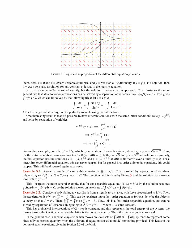
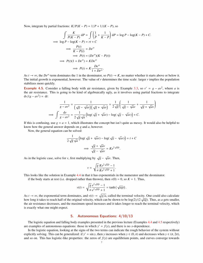
Figure 2. Logistic-like properties of the differential equation y′ = sin y.
them. here, y = 0 and y = 2π are unstable equilibria, and y = π is stable. Additionally, if y = g(x) is a solution, theny = g(x + c) is also a solution for any constant c, just as in the logisitc equation.
y′ = sin y can actually be solved exactly, but the solution is somewhat complicated. This illustrates the moregeneral fact that all autonomous equaations can be solved by a separation of variables: take dy/ f (y) = dx. This gives∫
dy/ sin y, which can be solved by the following trick: let u = cos y:∫dy
sin y=
∫sin y dy
sin2 y= −
∫du
1 − u2 .
After this, it gets a bit messy, but it’s perfectly solvable using partial fractions.One interesting result is that it’s possible to have different solutions with the same initial condition! Take y′ = y1/3,
and solve by separation of variables:
y−1/3 dy = dt =⇒y2/3
2/3= t + C
=⇒ y2/3 =2t3
+ C
=⇒ y =
(2t3
+ C)3/2
.
For another example, consider y′ = 1/y, which by separation of variables gives y dy = dt, or y = ±√
2t + C. Thus,for the initial condition corresponding to C = 0 (i.e. y(0) = 0), both y =
√2t and y = −
√2t are solutions. Similarly,
the first equation has the solutions y = −(2t/3)3/2 and y = (2t/3)3/2 at y(0) = 0; there’s even a third, y = 0. For alinear first-order differential equation, this can never happen, but for general first-order differential equations, this couldhappen. This will be discussed again next week.
Example 5.1. Anoher example of a separable equation is dydx = x/y. This is solved by separation of variables:
y dy − x dx¡ so y2/2 = x2/2 + C, or y2 − x2 = C. The direction field is given by Figure 3, and the solution can move onlevel sets of y2 − x2.
This illustrates the more general example. that for any separable equation A(x) dx = B(y) dy, the solution becomes∫A(x) dx −
∫B(y) dy = C, so the solution moves on level sets of
∫A(x) dx −
∫B(y) dy.
Example 5.2. Consider a body falling towards Earth from a significant distance, with force proportional to 1/r2. Then,the acceleration is c/r2, or d2r
dt2 = − cr2 . This can be rewritten into a first-order equation as follows: let v be the object’s
velocity, so that v′ = r′′. Then, dvdr
drdt = dv
dr v, so dvdr v = − c
r2 . Now, this is a first-order separable equation, and can besolved by separation of variables, integrating to v2/2 = c/r + C, where C is some constant.
This has a physical interpretation: v2/2 − c/r is constant, and this represents the total energy of the system: theformer term is the kinetic energy, and the latter is the potential energy. Thus, the total energy is conserved.
In the general case, a separable system which moves on level sets of∫
A(t) dt −∫
B(y) dy tends to represent somephysically conserved quantity when the differential equation is used to model something physical. This leads to thenotion of exact equations, given in Section 2.5 of the book:
8
Figure 3. Direction field for the equation y′ = x/y.
Definition. An exact equation is an equation for which one can find a “conserved quantity,” even if it isn’t separable.A large class of inseparable equations have some relatively obvious quantity that remains constant.
Example 5.3. This is a pretty contrived example, but shoud help illustrate the idea: y′ sin x + y cos x + 2x = 0. This is alinear equation, but it’s not separable, so one could solve it with an integrating factor. But there’a another, simpler way:the first two terms look like the derivative of a product y sin x, and the latter is the derivative of x2. Thus, the equationbecomes d
dx (y sin x + x2) = 0. Thus, y sin x + x2 is a constant, and from there it is easy to solve for y: y = (C − x2)/ sin x.Next time, we will discuss precisely how and when this sort of solution works.
6. Exact Equations: 4/12/13
With the techniques now developed, it will be possible to solve the pendulum equation given in Example 1.1. Recallthat the differential equation is
d2θ
dt2 +g`
sin θ = 0, (2)
where g is the acceleration due to gravity. This formula is due to calculating the forces and accelerations.This is a second-order equation, but can be broken into two first-order equations and thus solved: let v = dθ
dt , so thatd2θdt2 = dv
dt = dvdθ
dθdt = dv
dθv. Thus, the equation has simplified to
vdvdθ
+g`
sin θ = 0,
which is a separable first-order equation. Integrating,
v2
2=
g`
cos θ + C
=⇒v2
2−
g`
cos θ = C.
The left-hand side of the above equation is a conserved quantity, and is proportional to the energy. Then, substituting inthe initial condition θ = θ0, one can calculate that C = −g cos θ0/`, which when plugged back into the equation gives
v2
2=
g`
(cos θ − cos θ0)
v =
√2g`
(cos θ − cos θ0).
9

Thus, v is maximum when θ = 0 and is 0 when θ = θ0. However, in order to solve for θ there’s another equation tosolve, though once again it’s separable:
dθdt
=
√2g`
(cos θ − cos θ0)
=⇒
√`
2gdθ
√cos θ − cos θ0
= dt
There is no closed form for∫
dθ√
cos θ−a; such expressions are elliptic integrals. However, the period can still be calculated:
the time it takes the pendulum to go from angle θ0 to 0 is√`
2g
∫ θ0
0
dθ√
cos θ − cos θ0.
Thus, the total period is four times that. This is ugly, but works well for numerical approximations and such. However,when θ0 is small, the elliptic integral becomes approximately π/
√2, so the period is about 2π
√`/g. Of course, even the
“exact” formula doesn’t account for things like air resistance. The approximation can also be seen by taking sin θ ≈ θfor small θ in the original equation (2), and then solving the resulting linear equation.
An exact equation is an equation y′ = f (y, t), such that the goal is to find a function ψ(y, t)such that if y(t) is asolution of the equation, then ψ(y(t), t) is constant. Exact equations, discussed in Section 2.5 of the book, are those forwhich it is easy to find such a ψ, and include all separable equations.3
Example 6.1. Take 2t + y + (x + 3y2)y′ = 0. Then, ψ(y, t) = y3 + ty + t2, so that any solution y(t) satisfiesy(t)3 + ty(t) + t2 = C, giving an implcit expression for y(t).
Why does this work? Take the derivative:
dψdt
=ddt
(y3 + ty + t2) = 3y2 dydt
+ tdydt
+ y + 2t = 0,
because that was the differential equation posed at the head of the problem.In the general case, one has an equation M(y, t) + N(y, t)y′ = 0. Then, if ∂M
∂y = ∂N∂t , then there exists a function ψ(y, t)
such that ∂ψ∂t = M, ∂ψ
∂y = N, and ψ is constant along solutions, so if y(t) is a solution to the differential equation, thenψ(t, y(t)) is constant.
Though the specific method of finding these conserved quantities might not be useful, conserved quantities areextrenely important in general.
Returning to Example 6.1, M = 2t + y and N = t + 3y2, so ∂M∂y = 1 and ∂N
∂t = 1. Thus, such a ψ exists, but theresult cited above isn’t constructive. Fortunately, it’s not too difficult to find ψ: the goal is to find the function whosepartial derivatives are M and N. First, integrate ∂ψ
∂t = 2t + y with respect to t, treating y as a constant of integration.Thus, ψ = t2 + yt + C(y), since for each value of y, the constant of integration could be different. Similarly, integrating∂ψ∂t = t + 3y2, there’s a different constant (function) of integration: ψ = ty + y3 + D(t). Then, set these expressions equaland solve: y3 + D(t) = C(y) + t2, so ψ = ty + y3 + t2 + K, where K is an actual constant of integration.
Alternatively, after integrating the first equation, one could take ∂ψ∂y = t + dC
dy , and solve to obtain C. Note, however,that if the partial derivatives of M and N don’t agree, then this won’t work, as the two expressions for ψ will beincompatible.
The next example will show that separation of variables is a special case.Example 6.2. Suppose A(y) dy + B(t) dt = 0, or A(y)y′ + B(t) = 0. Thus, N(y, t) = A(y) and M(y, t) = B(t). Thus,∂M∂y = ∂N
∂t = 0. Thus, one can integrate: ψ =∫
A(y) dy +∫
B(t) dt = C for some constant C, once the above method isused, and this is exactly what separability already told us.
7. More Exact Equations: 4/15/13
Recall the defintion of an exact equation: a first order ODE M(x.y) + N(x.y)y′ = 0 is exact when Nx = My (partialderivatives). Thus, there is a function ψ(x, y) such that ∂ψ
∂y = N and ∂ψ∂x = M and if y = y(x) is a solution to the original
3The professor doesn’t actually think this is useful, and that it is in the syllabus of ODE courses largely by tradition. Admittedly, it is a powerfultechnique, but in the vast majority of cases, the equation is separable anyways, and worrying about exactness is needlessly complicated.
10
ODE, then ψ(x, y(x)) is constant. Then, one can sometimes solve for y(x) in terms of x, and even if not, it can be seenimplicitly.
Example 7.1. Suppose (2y + x2) dydx + (3x2 + 2xy) = 0. Then, N = 2y + y2 and M = 3x2 + 2xy. First, it is necessary
to check for exactness: ∂N∂x = 2x = ∂N
∂y , so we can proceed. The goal is to find a ψ such that ∂ψ∂y = 2y + x2 and
∂ψ∂x = 3x2 + 2xy.
Integrating the first equation with respect to y, ψ = y2 + x2y + C(x) for some function C of x, and integrating thesecond equation, ψ = x3 + x2y + D(y). Comparing these, C(x) = x3 and D(y) = y2, so ψ(x, y) = x3 + x2y + y2.4
Thus, if y(x) is a solution, then ψ(x, y(x)) is constant, so suppose y(0) = 1, so y(x)2 + x2y(x) + x3 = 1. This can besolved explicitly as y = (−x2 +
√x4 − 4x3 + 4)/2.
Why does this procedure work? If Ny′+ M = 0 and the partials agree, it’s necessary to check that the ψ defined abovealways exists, and that ψ(x, y(x)) is constant for every solution of the equation. Notice that for any twice-differentiablefunction g, ∂2g
∂x∂y =∂2g∂y∂x , so that order in evaluating partial derivatives doesn’t matter. Thus, if ψ exists, then ∂2ψ
∂x∂y = ∂N∂x
and ∂2ψ∂y∂x = ∂M
∂y , so the partials agree and ∂N∂x = ∂N
∂y . Then, if ψ(x, y(x)) is constant, then ddxψ(x, y(x)) = 0. This requires
using the two-variable chain rule:d fdx
=∂ f∂u
dudx
+∂ f∂v
dvdx
where f (u, v) and u and v are functions of x. Then, for ψ,dψdx
=∂ψ
∂x+∂ψ
∂ydydx
= M + Ndydx
= 0
by the given differential equation. Finally, it is necessary to establish why such a ψ should exist. See Theorem 2.5.1 inthe textbook for a more detailed discussion; the gist of it is that the integration method given always works: given Nand M, let ψ =
∫N dy + A(x), so that
∂ψ
∂x=
∂
∂x
(∫N dy + A(x)
)=
∫∂N∂x
dy +dA(x)
dx=
∫∂M∂y
dy +dAdx
= M(y) + B(x) + A′(x).
Thus, one can choose A(x) such that A′(x) + B(x) = 0, so that ∂ψ∂x = M(y) as needed.
Example 7.2. Suppose (2y/x + x)y′ + (3x − 2y) = 0. This isn’t exact: ∂N∂x = 1 − 2y/x2 and ∂M
∂y = 2. However, aftermultiplying by x, the equation from Example 7.1 is obtained, and the eqation can be solved.
In general, multiplying by an integrating factor can lead to solutions to more equations. The book has a morethorough discussion on this.
One can also talk about numerical solutions. This is covered in Section 2.6 of the book, and goes into quite a bit ofdetail. Most of it won’t be necessary for this class.Example 7.3. Let y′ = y2 and y(0) = 1. This can be solved exactly by separation of variables, where y = 1/(1 − x).This will be used so that the numerical value can be compared to the actual value: specifically, y(0.9) = 10.
Supposing this weren’t known, one could use Euler’s method to approximate y by the tangent line. y(0) = 1, soy(0, 1) ≈ y(0) + y′(0)(0.1) = 1.1, y(0.2) ≈ y(0.1) + y′(0.1)(0.1) = 1.21. Continuing in this way, y(0.9) ≈ 4.3.
This isn’t very good; how might it be done better? The most obvious solution is to increase the step size. Using stepsof 0.05, the approximation is y(0.9) ≈ 8.28, and if the step size is 0.001, the approximation is y(0.9) ≈ 9.78. This isactually close, but the tradeoff is that a lot more has to be calculated.
Thankfully, there are much better methods to approximate equations (e.g. using the tangent line in the midpoint ofan interval).
8. Numerical Methods and Existence and Uniqueness: 4/17/13
Return again to the equation y′ = y2, with y(0) = 1. The exact solution is y(x) = 1/(1 − x), but if this weren’tknown, how could it be approximated? Euler’s method was discussed in the previous lecture, but as shown, since eachaproximation depends on the previous one, this method becomes quite inacurate after repeated approximation. This canbe made better by reducing the step size. For exams, it’s helpful to know the basic idea, but in practice, there are muchbetter methods (which won’t be on the exam).
4Alternatively, after ψ = y2 + x2y + C(x) is obtained, one could differentiate with respect to x: ∂ψ∂x = 2xy + C′(x) = 3x2 + 2xy, so C′(x) = 3x2 and
C(x) = x3. The constant term will be irrelevant.11
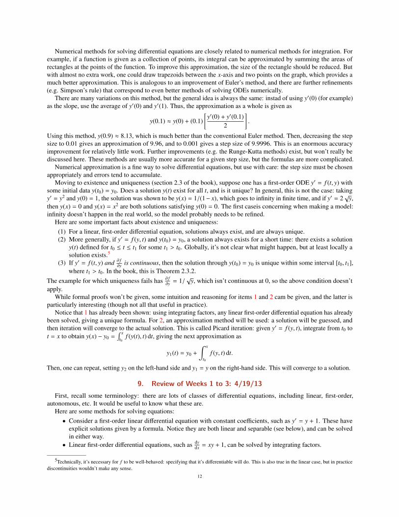
Numerical methods for solving differential equations are closely related to numerical methods for integration. Forexample, if a function is given as a collection of points, its integral can be approximated by summing the areas ofrectangles at the points of the function. To improve this approximation, the size of the rectangle should be reduced. Butwith almost no extra work, one could draw trapezoids between the x-axis and two points on the graph, which provides amuch better approximation. This is analogous to an improvement of Euler’s method, and there are further refinements(e.g. Simpson’s rule) that correspond to even better methods of solving ODEs numerically.
There are many variations on this method, but the general idea is always the same: instad of using y′(0) (for example)as the slope, use the average of y′(0) and y′(1). Thus, the approximation as a whole is given as
y(0.1) ≈ y(0) + (0.1)[y′(0) + y′(0.1)
2
].
Using this method, y(0.9) ≈ 8.13, which is much better than the conventional Euler method. Then, decreasing the stepsize to 0.01 gives an approximation of 9.96, and to 0.001 gives a step size of 9.9996. This is an enormous accuracyimprovement for relatively little work. Further improvements (e.g. the Runge-Kutta methods) exist, but won’t really bediscussed here. These methods are usually more accurate for a given step size, but the formulas are more complicated.
Numerical approximation is a fine way to solve differential equations, but use with care: the step size must be chosenappropriately and errors tend to accumulate.
Moving to existence and uniqueness (section 2.3 of the book), suppose one has a first-order ODE y′ = f (t, y) withsome initial data y(t0) = y0. Does a solution y(t) exist for all t, and is it unique? In general, this is not the case: takingy′ = y2 and y(0) = 1, the solution was shown to be y(x) = 1/(1− x), which goes to infinity in finite time, and if y′ = 2
√y,
then y(x) = 0 and y(x) = x2 are both solutions satisfying y(0) = 0. The first caseis concerning when making a model:infinity doesn’t happen in the real world, so the model probably needs to be refined.
Here are some important facts about existence and uniqueness:(1) For a linear, first-order differential equation, solutions always exist, and are always unique.(2) More generally, if y′ = f (y, t) and y(t0) = y0, a solution always exists for a short time: there exists a solution
y(t) defined for t0 ≤ t ≤ t1 for some t1 > t0. Globally, it’s not clear what might happen, but at least locally asolution exists.5
(3) If y′ = f (t, y) and ∂ f∂y is continuous, then the solution through y(t0) = y0 is unique within some interval [t0, t1],
where t1 > t0. In the book, this is Theorem 2.3.2.The example for which uniqueness fails has ∂ f
∂y = 1/√
y, which isn’t continuous at 0, so the above condition doesn’tapply.
While formal proofs won’t be given, some intuition and reasoning for items 1 and 2 cam be given, and the latter isparticularly interesting (though not all that useful in practice).
Notice that 1 has already been shown: using integrating factors, any linear first-order differential equation has alreadybeen solved, giving a unique formula. For 2, an approximation method will be used: a solution will be guessed, andthen iteration will converge to the actual solution. This is called Picard iteration: given y′ = f (y, t), integrate from t0 tot = x to obtain y(x) − y0 =
∫ xt0
f (y(t), t) dt, giving the next approximation as
y1(t) = y0 +
∫ x
t0f (y, t) dt.
Then, one can repeat, setting y2 on the left-hand side and y1 = y on the right-hand side. This will converge to a solution.
9. Review of Weeks 1 to 3: 4/19/13
First, recall some terminology: there are lots of classes of differential equations, including linear, first-order,autonomous, etc. It would be useful to know what these are.
Here are some methods for solving equations:• Consider a first-order linear differential equation with constant coefficients, such as y′ = y + 1. These have
explicit solutions given by a formula. Notice they are both linear and separable (see below), and can be solvedin either way.
• Linear first-order differential equations, such as dydx = xy + 1, can be solved by integrating factors.
5Technically, it’s necessary for f to be well-behaved: specifying that it’s differentiable will do. This is also true in the linear case, but in practicediscontinuities wouldn’t make any sense.
12
Example 9.1. Suppose y′ = y/x+. Since a linear differential equation looks like y′ = p(x)y + q(x), this islinear, and can be solved with integrating factors. Intutively, this can be thought of as a model in which p(x) issome sort of interest-like quantity, and q(x) represents some outside change. This isn’t essential, but having themodel is useful for intuition.
This can be solved by rewriting t as y′ − p(x)y = q(x) and multiplying by the integrating factor e−∫
p(x) dx.Then, this can be integrated: the integrating factor is M(x) = e−
∫1/x dx = e− log x = 1/x, so
1x
y′ −yx2 =
1x
=⇒ddx
( yx
)=
1x
yx
= log x + C
=⇒ y = x log x + Cx.
• Separable equations, such as y′ = y/x, can be solved by separation of variables.Example 9.2. Suppose y′ = x/y. Then, the idea in separation of variables is to move all x terms to one sideand all y terms to the other. This implies that y dy = x dx, which can be integrated:∫
x dx =
∫y dy
y2
2=
x2
2+ C
y2 = x2 + 2C
y = ±√
D + x2,
where D = 2C is a constant of integration determined by the initial conditions (e.g. if y(0) = 3, then D = 9 andthe sign of the square root is forced: y =
√9 + x2).
On the midterm, you may be asked to integrate things using partial fractions, integrating by parts, etc., butnothing overly tedious or tricky will be necessary.
• Separable equations can be further generalized to exact equations: M + Ny′ = 0, where ∂M∂X = ∂N
∂y . This implies
there is a function ψ(x, y) such that ∂ψ∂x = M and ∂ψ
∂y = N. ψ can be found by integrating, and leads to thesolutions: any solutiion of the original differential equation y = y(x) satisfies ψ(x, y(x)) is constant.
Example 9.3. Suppose 2xy4 + cos x + (4x2y3 + cos y) dydx = 0. First, this should be checked for exactness:
∂M∂y = ∂N
∂x = 8xy3, so this is in fact exact.
Then, ψ can be found by integrating: ∂ψ∂x = M, so ψ = x2y4 + sin x + f (y). Then, this can be plugged into
∂ψ∂y = N: ∂ψ
∂y = 4x2y3 + f ′(y) = N = 4x2y3 + cos y. Thus, f (y) = sin y + C, so ψ(x, y) = x2y4 + sin x + sin y, so ify = y(x) is a solution to the original differential equation, x2y4 + sin x + sin y is constant, and the specific valueis determined by the initial data.
Sometimes, an explicit solution in terms of y can be given; the above example doesn’t allow that, however.
Equations can be graphed as a slope field: if y′ = f (y, x), one can visualize solutions by following the slope field. Aspecial case happens for autonomous equations, where f is independent of x, and a graph can be visualized by justgraphing f (y). This leads to the idea of equilibrium solutions being stable or unstable. Since computers are so goodat graphing, there’s no reason to actually do this by hand, but the important concept is that solution trajectories willfollow these direction fields. For an autonomous equation, looking at f (y) indicates where the solution is increasing ordecreasing.
An equilibrium solution, corresponding to a zero of an autonomous equation, is a constant solution to the equation(e.g. y(t) = kπ for k ∈ Z when y′(x) = sin x). Here, y = 0 is an unstable solution: a small perturbation leads to differentlong-term behavior, but y = π is stable: nearby solution curves are pulled in.
Sometimes, a solution may be neither stable nor unstable, in which case it is called semistable. If y′(x) = x2, theny = 0 is semistable: solution curves below it converge to it, but those above it diverge.
As for numerical solutions, there is Euler’s method, which approximates a solution by its tangent line, and severalbetter approximations, but only Euler’s method will be tested.
13
Existence and uniqueness: for linear, first-order equations, solutions exist and are unique given some initial data. Inthe general case, however, all that is known is that solutions exist locally and they might not be unique. Relatedly, y cango to infinity in a finite time.
10. Systems of Differential Equation: 4/22/13
For the next three weeks, this course will look at systems of differential equations. An example of this is dxdt = x + y2
and dydt = y − x. Given x(0) = 3 and y(0) = 1, what are x(t) and y(t)? For another example, suppose dx
dt = x + y + z,dydt = y − z, and dz
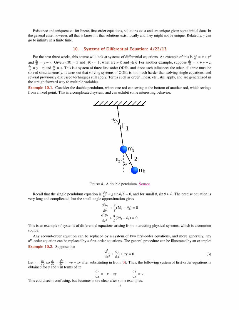
dt = x. This is a system of three first-order ODEs, and since each influences the other, all three must besolved simultaneously. It turns out that solving systems of ODEs is not much harder than solving single equations, andseveral previously discussed techniques still apply. Terms such as order, linear, etc., still apply, and are generalized inthe straightforward way to multiple variables.Example 10.1. Consider the double pendulum, where one rod can swing at the bottom of another rod, which swingsfrom a fixed point. This is a complicated system, and can exhibit some interesting behavior.
Figure 4. A double pendulum. Source
Recall that the single pendulum equation is d2θdt2 + g sin θ/` = 0, and for small θ, sin θ ≈ θ. The precise equation is
very long and complicated, but the small-angle approximation gives
d2θ1
dt2 +g`
(2θ1 − θ2) = 0
d2θ2
dt2 +g`
(2θ2 − θ1) = 0.
This is an example of systems of differential equations arising from interacting physical systems, which is a commonsource.
Any second-order equation can be replaced by a system of two first-order equations, and more generally, anynth-order equation can be replaced by n first-order equations. The general procedure can be illustrated by an example:Example 10.2. Suppose that
d2ydx2 +
dydx
+ xy = 0. (3)
Let v =dydx , so dv
dx =d2ydx2 = −v − xy after substituting in from (3). Thus, the following system of first-order equations is
obtained for y and v in terms of x:dvdx
= −v − xydydx
= v.
This could seem confusing, but becomes more clear after some examples.14
Similarly, for higher-order equations, one makes substitutions for higher-order derivatives. If y′′ + y′ + y − x = 0,then one makes the substitution v = y′ and u = y′′ to obtain a system of three first-order equations.
Just as the general form for a first-order ODE is y′ = f (x, y), the general form of a system of two first-order equationsis du
dx = f1(x, u, v), and dvdx = f2(x, u, v). Similarly, a first-order linear equation looks like y′ = p(x)y + q(x), and in the
case of two equations is generalized todudx
= a(x)u + b(x)v + e(x)
dvdx
= c(x)u + d(x)v + f (x).
Example 10.3. Consider the motion of the Earth around the Sun. From F = ma, one obtains
d2xdt
=−Cx
(x2 + y2)3/2 andd2ydt
=−Cy
(x2 + y2)3/2 ,
where the Sun is at the origin and the Earth traces out the trajectory (x(t), y(t)). This is a system of nonlinear, second-order differential equations, and is kind of complicated. Another example of where systems arise is when an object hasmore than one degree of freedom.Example 10.4. Suppose one has a chemical reaction A + B → C. Let a(t) be the amount of molecule A presentat time t, and similarlly for b(t) and B, and c(t) and C. A typical rate law for the reaction is da
dt = −Ca(t)b(t), anddbdt = −Ca(t)b(t) as well,6 giving a system of first-order, nonlinear dfferential equations. This is a nuance: products ofthe two dependent variables are not allowed in a system of linear equations. This equation can actually be solved byconverting it to a single equation and then using separation of variables.
An important way to understand these systems is to think of them in the linear-algebraic sense: if dxdt = 2x + y + t and
dydt = x − 2y + t2, then this can be rewritten in matrix notation: dV
dt = PV + Q, where the product is matrix multiplication,
and V(t) =
[x(t)y(t)
], P =
[2 11 2
], and Q =
[tt2
]. Using this formalism, many of the previous solution methods will apply,
but with scalars replaced with matrices. This can be seen by explicitly computing PV + Q, which will evaluate to[ dxdtdydt
]=
[2x + y + tx + 2y + t
],
which is the same system, but written in a way that looks much more like the previous examples.
Example 10.5. Suppose dxdt = 2x + y and dy
dt = x = 2y. This system can be solved from the matrix viewpoint. First, asustitution will be made: though it looks like it comes from nowhere, it will be explained in a future lecture. It has to dowith eigenvectors, but don’t worry about that yet; it will make sense. Let x = u + v and y = u − v, which gives
dudt
+dvdt
= 2(u + v) + (u − v) anddudt−
dvdt
= (u + v) + 2(u − v).
Then, u and v can be obtained, and the reverse substitution can be made in the end. Then, the equations simplify,dudt = 3u and dv
dt = v after solving. Now, these two equations are completely independent, and can be solved separately:u(t) = C1e3t and v(t) = C2et. Thus, x(t) = C1e3t + C2et and y = C1e3t −C2et.
11. Review of Linear Algebra: 4/24/13
In order to solve systems of linear equations, eigenvalues and eigenvectors are necessary to obtain good coordinatesfor the system, so they will be reviewed.
Let A be a 2 × 2 matrix. Everything will generalize nicely to n × n, but this will have easier intuition.
Definition. The determinant of a matrix is det[a bc d
]= ad − bc.
This indicates how the area of a region changes under action by A: if R ⊂ R2 and A(R) = R′, then area(R′) =
| det A| area(R). This formula will not be used much in this course, but it’s important in order to understand what thedeterminant does. Here are some facts about the determinant:
• If det A , 0, then A is invertible; that is, there exists a matrix A−1 such that AA−1 = A−1A = I.
6There are plenty of reactions where more complicated rate laws exist, because of some sort of intermediate process. However, the equationsgiven above are correct for many reactions.
15
• if det A = 0, then A has a null space; that is, there is a nonzero vector v =
[v1v2
]such that Av = 0.
Definition. A vector v =
[v1v2
]is called an eigenvector of A if Av is a scalar multiple of v, or Av =
[v1v2
]= λ
[v1v2
].
Then, λ is called an eigenvalue of A.
Example 11.1. If A =
[2 11 2
], then v =
[11
]is an eigenvector with eigenvalue 3, because
A[11
]=
[2 11 2
] [11
]=
[33
]= 3v.
Additionally, v =
[1−1
]is an eigenvector with eigenvalue 1.
Eigenvectors are important in differential equations because every eigenvector of A gives a solution to the differential
equationddt
[xy
]= A
[xy
]. Specifically, let v =
[v1v2
]be an eigenvector of A with eigenvalue λ. Then, x = v1eλt and
y = v2eλt is a solution to the indicated differential equation. One can also think of this as[xy
]= veλt.
Example 11.2. When A =
[2 11 2
]and v =
[11
], then x = e3t and y = e3t is a solution, by Example 11.1
Why does this method work? Set[xy
]= veλt =
[v1eλt
v2eλt
], and it will be shown that it satisfies the equation:
ddt
[xy
]=
ddt
[v1eλt
v2eλt
]=
[λv1eλt
λv2eλt
]= λeλt
[v1v2
].
A[xy
]= Aveλt = λveλt.
Thus, the equation is satisfied. These turn out to give all possible solutions, as will be seen later.Returning to the review of linear algebra, suppose λ is an eigenvalue of A. Then, Av = λv = λIv, so (A − λI)v = 0.
Then, take the determinant: det(A − λI) = 0 is a quadratic polynomial in λ whose roots yield the eigenvalues of A. Thisis called the characteristic polynomial of A.
In the case of the matrix A from Example 11.1, det(A − λI) = (2 − λ)2 − 1. Thus, λ = 1 and λ = 3 are the twoeigenvalues.
There are some wrinkles in this solution process: the eigenvalues could be complex or repeated. This is fine, but willhave to be dealt with later.
Assuming these issues don’t pop up, the eigenvectors can be found: if Av = λ1v, then (A − λ1I)v = 0, so theeigenvectors are the null space of A − λ1I.
For the matrix A we’ve been working with, an eigenvector for λ1 = 3 is in the null space of[−1 11 −1
], so v =
[11
]works, as does any scalar multiple of it.
Now, it is possible to obtain the general solution toddt
[xy
]= A
[xy
]. This is the analogue to the linear equation with
constant coefficients. This will correspond to Theorems 3.3.1 and 3.3.2 in the book. For now, assume the eigenvalues ofA are distinct: λ1 , λ2, and let v1 and v2 be the corresponding eigenvectors. Then, the general solution is[
xy
]= c1eλ1tv1 + c1eλ2tv2,
where c1 and c2 are constant determined by the initial conditions. Note that λ1 and λ2 might be complex, and that theircorresponding eigenvectors also might have complex entries.
It turns out that all solutions of the equation come from these eigenvalues. First observe that the solution can berewritten as [
xy
]= eAt
[b1b2
]for some constants b1 and b2. However, this involves taking the exponential of a matrix. . . which is in fact a perfectlylegitimate operation.
16
Definition. If M is a square matrix, then its exponential can be given by two equivalent definitions:
eM = limn→∞
(I +
Mn
)n
= 1 + M +M2
2+ · · ·
This is advantageous because it allows the solution to be rewritten so that it looks like the single-variable case.However, it requires computing the matrix exponential, which in practice boils down to the same eigenvalue andeigenvector calculations as before.
12. Systems of Linear Equations: 4/26/13
Recall that the differential equationddt
[xy
]= A
[xy
]has the general solution
[xy
]= c1v1eλ1t + c2v2eλ2t, where λ1 and
λ2 are the distinct eigenvalues of A and v1 and v2 are their corresponding eigenvectors. However, this compact solutioncontains a lot of information: λ1, λ2 > 0 looks very different to when they have opposite sign, or when they are complex,etc.
The derivation can be understood by setting U = [v1 v2], and make the substitution[xy
]= U
[uv
]. Then, the equation
becomes dudt = λ1u and dv
dt = λ2v, which is easy to solve. This is because AU = [Av1 Av2] = [λ1v1 λ2v2].
Example 12.1. If dxdt = 2x + y and dy
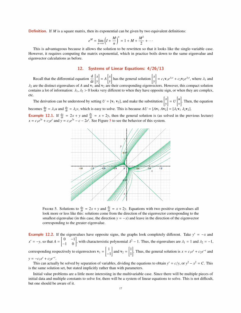
dt = x + 2y, then the general solution is (as solved in the previous lecture)x = c1e3t + c2et and y = c1e3t − c − 2et. See Figure 5 to see the behavior of this system.
Figure 5. Solutions to dxdt = 2x + y and dy
dt = x + 2y. Equations with two positive eigenvalues alllook more or less like this: solutions come from the direction of the eigenvector corresponding to thesmallest eigenvalue (in this case, the direction y = −x) and leave in the direction of the eigenvectorcorresponding to the greater eigenvalue.
Example 12.2. If the eigenvalues have opposite signs, the graphs look completely different. Take y′ = −x and
x′ = −y, so that A =
[0 −1−1 0
], with charactersistic polynomial λ2 − 1. Thus, the eigenvalues are λ1 = 1 and λ2 = −1,
corresponding respectively to eigenvectors v1 =
[1−1
]and v2 =
[11
]. Thus, the general solution is x = c1et + c2e−t and
y = −c1et + c2e−t.This can actually be solved by separation of variables, dividing the equations to obtain y′ = c/y, or y2 − x2 = C. This
is the same solution set, but stated implicitly rather than with parameters.Initial value problems are a little more interesting in the multivariable case. Since there will be multiple pieces of
initial data and multiple constants to solve for, there will be a system of linear equations to solve. This is not difficult,but one should be aware of it.
17
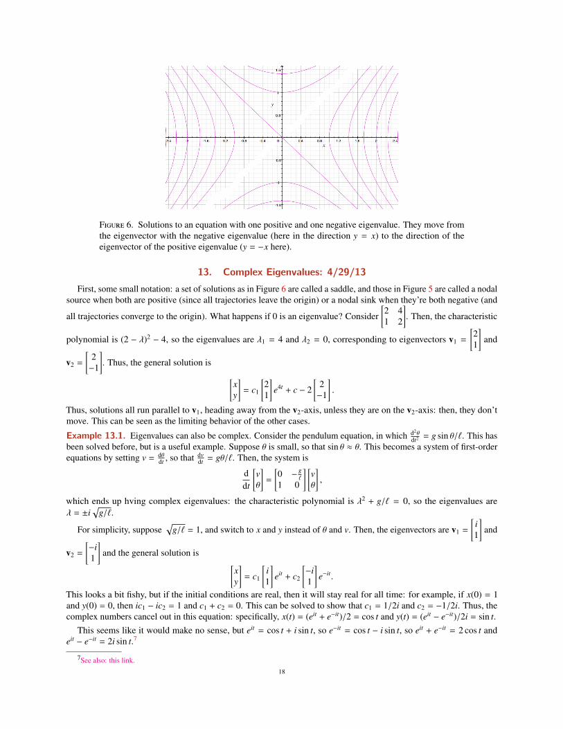
Figure 6. Solutions to an equation with one positive and one negative eigenvalue. They move fromthe eigenvector with the negative eigenvalue (here in the direction y = x) to the direction of theeigenvector of the positive eigenvalue (y = −x here).
13. Complex Eigenvalues: 4/29/13
First, some small notation: a set of solutions as in Figure 6 are called a saddle, and those in Figure 5 are called a nodalsource when both are positive (since all trajectories leave the origin) or a nodal sink when they’re both negative (and
all trajectories converge to the origin). What happens if 0 is an eigenvalue? Consider[2 41 2
]. Then, the characteristic
polynomial is (2 − λ)2 − 4, so the eigenvalues are λ1 = 4 and λ2 = 0, corresponding to eigenvectors v1 =
[21
]and
v2 =
[2−1
]. Thus, the general solution is [
xy
]= c1
[21
]e4t + c − 2
[2−1
].
Thus, solutions all run parallel to v1, heading away from the v2-axis, unless they are on the v2-axis: then, they don’tmove. This can be seen as the limiting behavior of the other cases.
Example 13.1. Eigenvalues can also be complex. Consider the pendulum equation, in which d2θdt2 = g sin θ/`. This has
been solved before, but is a useful example. Suppose θ is small, so that sin θ ≈ θ. This becomes a system of first-orderequations by setting v = dθ
dt , so that dvdt = gθ/`. Then, the system is
ddt
[vθ
]=
[0 −
g`
1 0
] [vθ
],
which ends up hving complex eigenvalues: the characteristic polynomial is λ2 + g/` = 0, so the eigenvalues areλ = ±i
√g/`.
For simplicity, suppose√
g/` = 1, and switch to x and y instead of θ and v. Then, the eigenvectors are v1 =
[i1
]and
v2 =
[−i1
]and the general solution is [
xy
]= c1
[i1
]eit + c2
[−i1
]e−it.
This looks a bit fishy, but if the initial conditions are real, then it will stay real for all time: for example, if x(0) = 1and y(0) = 0, then ic1 − ic2 = 1 and c1 + c2 = 0. This can be solved to show that c1 = 1/2i and c2 = −1/2i. Thus, thecomplex numbers cancel out in this equation: specifically, x(t) = (eit + e−it)/2 = cos t and y(t) = (eit − e−it)/2i = sin t.
This seems like it would make no sense, but eit = cos t + i sin t, so e−it = cos t − i sin t, so eit + e−it = 2 cos t andeit − e−it = 2i sin t.7
7See also: this link.18

This gives another way to write the general solution: if λ1 is complex and corresponds to eigenvalue v1, then insome sense these contain all of the necessary information for the other eigenvalue: the general solution can be writtenc1 Re(v1eλ1t) + c2 Im(v1eλ1t). Both equations are valid for any equation, but the constants will be different.
In Example 13.1 discussed above, this second form can be found as
v − 1eλ1t =
[i1
]eit =
[i(cos t + i sin t)cos t + i sin t
]=
[− sin t + i cos tcos t + i sin t
],
so the general solution is c1
[− sin tcos t
]+ c2
[cos tsint
].
14. Complex Exponentials: 5/1/13
Recall that if the eigenvalues of A are complex (if one is, then the other is), then the general solution to ddt
[xy
]= A
[xy
]is
[xy
]= c1 Re(v1eλ1t) + c2 Im(v1eλ1t). These solutions tend to have trigonometric functions in the solution, and in some
sense they oscillate. Also, note the lack of λ2 or v2 in the solution: their information can be extracted from λ1 and v1.Since the complex exponential comes up so often, it’s worth reviewing. The goal is to understand that eit =
cos t + i sin t, which is called Euler’s formula. The picture is that eit lives on the unit circle in the complex numbers. Fora plausibility argument, recall that cos(x + y) = cos x cos y + sin x sin y and sin(x + y) = sin x cos y + sin y cos x. Thus, ifg(x) = cos x + i sin x, so
g(x)g(y) = (cos x + i sin x)(cos y + i sin y)− (cos x cos y − sin x sin y) + i(sin x cos y + cos x sin y)= g(x + y).
There are several proofs of this formula, including a geometric one.
Proof 1. Set g(x) = cos x + i sin x as before and f (x) = eix. Then, d fdx = ieix = i f (x) and dg
dx = − sin x + i cos x = ig(x).Thus, both f and g satisfy the differential equation y′ = iy. Additionally, they have the same initial conditions:f (0) = g(0) = 1. Thus, by uniqueness of differential equations, f (x) = g(x). �
The second proof is more historical, and is due to Euler:
Proof 2. Write out the Taylor expansions of f and g and of cos x and sin x: ex =∑∞
n=0 xn/n!, so
eix =
∞∑n=0
inxn
n!=
∞∑n=0
(−1)2nx2n
(2n)!+ i
∞∑n=0
(−1)2n+1x2n+1
(2n + 1)!= cos x + i sin x. �
Example 14.1. Suppose A =
[8 −52 1
]and d
dt
[xy
]= A
[xy
], with the initial condition
[x(0)y(0)
]=
[12
]. This will be a more
representative example of the case of complex eigenvalues than Example 13.1. Then, the characteristic polynomial isλ2 − 4λ + 13 = 0, so λ1 = 2 + 3i and λ2 = 2 − 3i. Notice that the eigenvalues are complex conjugates of each other:λ2 = λ1 (recall that a + bi = a − bi). This is because a quadratic polynomial with one (strictly) complex root has twocomplex roots that are conjugates of each other, and the determinant is given by a polynomial.
The eigenvectors also exhibit this behavior: after some computation, v1 =
[1 + 3i
2
](though any multiple of v1 works,
even complex multiples). Since λ2 = λ1, then v2 = v1, so v2 =
[1 − 3i
2
]. This is why v2 and λ2 don’t appear in the
general solution. Thus,
v1eλ1t =
[1 + 3i
2
]e(2+3i)t = e2t
[(1 + 3i)(cos 3t + i sin 3t)
2(cos 3t + i sin 3t)
],
so the general solution is [xy
]= c1
[e2t(cos 3t − 3 sin 3t)
2e2t cos 3t
]+ c2
[e2t(3 cos 3t + sin 3t)
2e2t sin 3t
].
19
Unfortunately, this sort of messiness tends to be inevitable. With the initial conditions, c1 = 1 and c2 = 0, so[xy
]=
[e2t(cos 3t − 3 sin 3t)
2e2t cos 3t
]. Notice that a real differential equation with a real initial condition has a real solution.
Geometrically, this graph oscillates, but the oscillations in the x- and y-directions are staggered, and the exponentialterm causes them to increase. This can be rewritten to make the lag clearer: 1 + 3i =
√10eiθ, where θ = arctan 3 ≈ 71◦.
This indicates exactly what the lag is.
15. Repeated Eigenvalues: 5/6/13
Example 15.1. Recall the double pendulum equation from Example 10.1, which was given by
d2θ1
dt2 =g`
(−2θ1 + θ2)
d2θ2
dt2 =g`
(2θ1 − 2θ2).
This will be solved by breaking it into a system of four first-order equations: let u = θ′1 and v = θ′2, and suppose g/` = 1for ease of algebra. The four equations are
dθ1
dt= u
dθ2
dt= v
dudt
= −2θ1 + θ2dvdt
= 2θ1 − 2θ2
which gives the matrix
ddt
θ1θ2uv
=
0 0 1 00 0 0 1−2 1 0 02 −2 0 0
θ1θ2uv
.All of the theory still works, but there will be four eigenvalues rather than two. In particular, the general solution isgiven by
θ1θ2uv
=
4∑i=1
civieλit,
where λ1, . . . , λ4 are the eigenvalues and v1, . . . , v4 are their corresponding eigenvectors.After some unfortunate algebra, the characteristic polynomial is λ4 + 4λ2 + 2 = 0. Thus, the solutions are given by
the roots of −2 ±√
2, and are thus λ = ±i√
2 +√
2 ≈ 1.848i and λ = ±i√
2 −√
2 ≈ 0.765i. For general g, `, these are
instead λ = ±i√
g/`√
2 ±√
2. Thus, the solutions will be given by sines and cosines of 1.848√
g/`t and 0.765√
g/`t.Physically, this means that there are two modes of oscillation with different frequencies 1.848
√g/` and 0.765
√g/`,
and a typical solution will combine both modes, so it’s not as obvious that it is periodic. Compare with the singlependulum, which only has frequencies
√g/`.
In all of the cases mentioned before, there was a caveat that eigenvalues cannot be repeated. What happens if theyare?
Example 15.2. Supposeddt
[xy
]=
[1 10 1
] [xy
], so the eigenvalues are λ = 1, 1 given by a repeated root. Then, v =
[10
]is an eigenvector, so cveλt is a solution, but it’s not the completely general solution.
Notice that one of the equations doesn’t depend on x. This is no coincidence: in a system of repeated eigenvalues,this tends to happen. Thus, y(t) = et if y(0) = 1 and x(0) = 1, so we also have dx
dt = x + et. This can be solved with theintegrting factor e−t, yielding e−t dx
dt − e−t x = 1, so e−t x = t + C. and x = tet + et.
There’s another way to solve the system: look instead atddt
[xy
]=
[a 10 1
] [xy
], where a ≈ 1. This shouldn’t have
repeated eigenvalues, but will approach the solution we look for when a → 1. Here, the eigenvalues are λ1 = 1 and20
λ2 = a, and the eigenvectors are v1 =
[1
1 − a
]and v2 =
[10
]. Thus, the general solution is
[xy
]= c1
[1
1 − a
]et + d
[10
]eat.
With the initial conditions x(0) = y(0) = 1, d = 1 − 1/(1 − a), which goes to infinity as a → 1. However, c and dwill sort of cancel each other out, so that there is a valid solution: when a → 1, y(t) → et, which is fine, and thenx(t) = eat + (ret − eat)/(1 − a), so as a→ 1, x(t)→ et + teat/1.
More generally, suppose A has only one eigenvalue λ and that A is not diagonal (which is an easy case anyways).
Then, the general soluton to x′ = Ax is[xy
]= wteλt + veλt, where w is an eigenvector of λ and Av − λv = w. The
apparent lack of constants is because they can be absorbed into the eigenvector.
16. Variation of Parameters I: 5/8/13
Though this has a new name, this is just the use of integrating factors in the context of systems of differentialequations.
Up to now, the only systems that have been considered are homogeneous, where there are no terms just in t. Aninhomogeneous system is one of the form
ddt
[xy
]= A
[xy
]+
[f (t)g(t)
].
Recall that if dxdt = 3x + et, the integrating factor is e−3t, which can be multiplied in. But one can alternately make a
substitution x = e3tu, which turns the equation into dudt = e2u. For systems, the exponential in the integrating factor (or
substitution) is replaced by a matrix exponential.
To solve a system ddt v = Av + f, where v =
[x(t)y(t)
]and f =
[f (t)g(t)
], then a substitution v = X(t)u, where X(t) is a
2 × 2 matrix, and then the objective is to solve for u. The goal is to choose X to make life simpler (X = eAt will work).Specifically, after substitution, X(t) du
dt + dXdt u = AXu + f, since the product rule still holds on matrices. After simplifying,
X dudt = f, or du
dt = X−1f. Thus, u =∫
X−1f dt, where X and f both depend on t. Thus, the general solution to dvdt = Av + f
is
v(t) = X(t)∫
X(t)−1f(t) dt,
where X(t) satisfies ddt X(t) = AX(t). In order to actually obtain X, solve dx
dt = Ax, obtaining two vector solutions x1 =[x1(t)y1(t)
]and x2 =
[x2(t)y2(t)
]. It is necessary that these solutions be independent. Then, X(t) = [x1(t) x2(t)] =
[x1(t) y1(t)x2(t) y2(t)
].
Notice that the f term is ignored in this calculation. The idea here is that if it’s possible to solve the equation without f,then it is possible to solve with f just as easily.Example 16.1. Suppose
ddt
[xy
]=
[2 11 2
] [xy
]+
[10
]. (4)
Then, A has eigenvalues λ1 = 3 and λ2 = 1, corresponding to eigenvectors v1 =
[11
]and v2 =
[1−1
]. A general solution
to the homogeneous equation is x(t) = c1
[11
]e3t + c1
[1−1
]et, so two independent solutions are
[e3t
e3t
]and
[et
e−t
], so
X =
[e3t et
e3t e−t
]. Thus, the general solution to (4) is X(t)
∫X(t)−1
[10
]dt, which is just algebra. To specifically obtain
X−1f, one could compute the matrix inverse, but a potentially less error-prone method is to solve Xy = f for y, which isa conventional linear, non-differential system. The inverse of a 2 × 2 matrix can be given by an explicit formula:
B−1 =
[a bc d
]−1
=1
det B
[d −b−c a
],
21
where the determinant is det B = ad − bc. Thus, det X(t) = −2e4t, so
X−1 =1−2e4t
[−et −et
−e3t e3t
]=
[ 12 e−3t 1
2 e−3t
12 e−t − 1
2 e−t
],
so X−1f =
[e−3t/2w−t/2
]. Then, the vetor can be integrated termwise, and
∫X(t)f dt =
[−e−3t/6−e−t/2
]+
[c1c2
]. Then, the general
solution is found by multiplying this by X again.
17. Variation of Parameters II: 5/10/13
Example 17.1. Suppose A =
[2 11 2
], which has eigenvalues λ1 = 3 and λ2 = 1 and eigenvectors v1 =
[11
]and
v2 =
[1−1
]/ Then, the general solution to x′ = Ax is c1
[11
]e3t + c2
[1−1
]et. Then, let
[x1y1
]=
[e3t
e3t
]and
[x2y2
]=
[et
e−t
], so that
X(t) =
[e3t et
e3t e−t
].
Then, to solve the system ddt
[xy
]= A
[xy
]+
[10
], variation of parameters can be used. det = −2e4t, so X(t)−1 =
1det X
[−et −et
−e3t e3t
], so that X−t
[10
]=
[e−3t/2e−t/2
], so the general solution is[
xy
]= X(t)
∫ [e−3t/2e−t/2
]= X(t)
[−e−3t/6 + c1−e−t/2 + c2
]=
[−2/31/3
]+ c1
[e3t
e3t
]+ c2
[et
e−t
].
Notice that the general solution for the inhomogeneous equation is the general solution for the inhomogeneous solutionplus some additional data.
Alternatively, if ddt
[xy
]= A
[xy
]+
[et
0
], then X(t)
[et
0
]=
[e−2t/21/2
](which can also be found by Xy = f if you don’t want
to compute X−1), so the general solution is
X(t)[−e−2t/4 + c1
t/2 + c2
]=
[−et/4 + tet/2−et/4 − tet/2
]+ c1
[e3t
e3t
]+ c2
[et
e−t
].
In order to invert X(t), it’s necessary to compute its determinant. This happens to be simpler than in the general case,motivating the idea of a Wronskian.
Definition. If v1(t) =
[x1(t)y1(t)
]and v2(t) =
[x2(t)y2(t)
]are solutions to the homogeneous equation d
dt
[xy
]= A
[xy
], then the
Wronskian of v1 and v2 is
W(t) = det[x1(t) x2(t)y1(t) y2(t)
]= ke(a+d)t,
where k is some constant and A =
[a bc d
].
This is modtly helpful when the differential equation is messy.
Example 17.2. Suppose A =
[0 1−1 0
], for which a general solution is c1
[sin tcos t
]+ c2
[cos t− sin t
]. Then, the Wronskian of[
sin tcos t
]and
[cos t− sin n
]is det
[sin t cos tcos t − sin t
]= − sin2 t − cos2 t = −1 as predicted.
The reason this makes sense is that the Wronskian satifies the differential equation W ′(t) = (a + d)W(t), which is asimple differential equation and yields the formula given above. This is because the determinant is given by x1y2 − x2y1,so using the product rule,
W ′(t) = x′1y2 + x1y′2 − x′2y1 − x2y′1= (ax1 + by1)y2 + x1(cx2 + dy2) − (ax2 + by2)y1 − x2(cx1 + dy1)= (a + d)(x − 1y2 − x2y1) = (a + d)W(t),
after some messy algebra and using the fact that x′ = Ax. This can be generalized to larger systems, and is even valid ifthe entries in A depend on t.
22
Definition. Suppose v1 and v2 are two solutions of an equation and X(t) = [v1 v2]. Then, they are said to beindependent if their Wronskian is nonzero.
The following statements are equivalent:
(1) v1 and v2 are a fundamental set of solutions.(2) v1 is not a multiple of v2.(3) X(t) is invertible for all t.(4) Any solutin to the equation is of the form c1v1(t) + c2v2(t).
Example 17.3. If A is as in Example 17.2, then v1 =
[sin tcos t
]and v2 =
[cos t− sin t
]has Wronskian −1 and is thus a
fundamental set of solutions. There are many such sets; take v2 as before and v1 =
[sin t + cos tcos t − sin t
], so that the Wronskian
is still the same. However,[sin tcos t
]and
[2 sin t2 cos t
]is not such a soluton set.
18. Review of Weeks 4 to 6: 5/13/13
Suppose ddt
[xy
]= A
[xy
], for some 2 × 2 matrix that doesn’t depend on A. Then, suppose λ1, λ2 are distict eigenvalues
of A corresponding to eigenvectors v1, v2 respectively, then the general solution is c1v1eλ1t + c2v2eλ2t. This workswhether the eigenvalues are real or complex.
If λ − 1 = λ2 and A isn’t diagonal (which is an easy case, because the equations are unrelated), then let v1 be aneigenvector and v2 be given by Av2 − λv2 = v1. Then, the general solution is c1v1teλ1t + (c1v2 + c2v1)eλ1t. Alternatively,this can be given as uteλ1t + weλ1t, for every eigenvector u and every solution w to Aw − λ1w = u.
If λ1 and λ2 are complex, then they are conjugates of each other, as are v1 and v2, soa general solution is c1 Re(v1eλ1t)+c2 Im(v1eλ1t), which can be made more real by taking eiθ = cos θ + i sin θ.
If λ1 > λ2 > 0, then the phase portrait (what happens geometrically), solutions proceed from the direction of theeienvector corresponding to the smaller eigenvalue and proceed to the eigenvector corresponding to the larger eigenvalue.This is known as a nodal source. If both eigenvalues are negative, the trajectories are reversed, and converge at zero.This is called a nodal sink.
If the eigenvalues have opposite signs, the solutions form hyperbolas with the eigenvectors as the asympotes. This iscalled a saddle. If λ2 = 0, then the trajectories are just lines perpendicular to v2.
In the case of repeated eigenvalues, there are spirals that start pointing in one direction of v1 and end up pointingin the other. This is called an improper nodal source, and can be thought of as the limit of the nodal source as theeigenvectors appproach each other.
In the case of complex eigenvalues, λ1, λ2 = α ± iβ. If α > 0, then trajectories spiral away from the origin, and thegraph is called a spiral source. This corresponds to oscillations of increasing magnitude. if α < 0, then one has a spiralsink: the trajectories converge to zero, corresponding to oscilaltions of decreasing magnitude. In order to determinewhether the spirals travel clockwise or counterclockwise, it is necessaery to compute a sample direction in the directionfield; then, all trajectories will travel in that direction.
For variation of parameters, consider an inhomogeneous equation ddt
[xy
]= A
[xy
]+
[f (t)g(t)
], where A is a 2 × 2 real
matrix. Then, one finds two solutions[x1(t)y1(t)
]and
[x2(t)y2(t)
]of the homogeneous equation x′ = Ax, and take the matrix
X(t) =
[x1(t) x2(t)y1(t) y2(t)
]. The Wronskian of these two vectors is W(t) = det(X(t)) = Ce(Tr A)t. If the Wronskian is nonzero,
then these two solutions are called a fundamental set (i.e. they are independent of each other). Then, the general solution
is X(t) =∫
X(t)−1[
f (t)g(t)
]dt when the Wronskian is nonzero (so that the inverse makes sense). Once again, there could
be complex eigenvalues. The general solution to the homogeneous equation will be part of the answer. As it happens,this method works just as well in the case of repeated eigenvalues.
One convenient formula for X−1 is X−1 = (Tr X)(I − X)/ det X.23

Example 18.1. This example will demonstrate the calculation of the Wronskian of a matrix with repeated eigenvalues:
suppose A =
[1 10 1
], which has λ = 1 as its sole eigenvalue, for which an eigenvector is v =
[10
]. Solving Av2−λv2 = v1,
one obtains v2 =
[01
]. Thus, the general form of solutions to the homogeneous equation is c−1
[1t
]et +
(c1
[01
]+ c2
[10
])et,
so take c1 = 1 and c2 = 0 to obtain[x1y1
]=
[tet
et
]and for the second c1 = 0 and c2 = 1 to obtain
[x2y2
]=
[et
0
]. Thus, the
Wronskian is
∣∣∣∣∣∣tet et
et 0
∣∣∣∣∣∣ = −e2t.
19. Second Order Linear Systems: 5/15/13
Today’s lecture will consider second-order, linear equations
a(x)d2ydx2 + b(x)
dydx
+ c(x)y = d(x).
Generall,y the equations will be taken to have a, b, c constant, such as 2y′′ + y′ + 3y = 0. More generally, it will bepossible to obtain a general solution to ay′′ + by′ + cy = 0, which arises often in oscillating systems.
First, reduce the equation to two fist-order equations: let v = y′, so v′ = (−b/a)v − (c/a)y, leading to a system
ddx
[yv
]=
[0 1− c
a − ba
] [yv
],
which has characteristic polynomial aλ2 + bλ + c = 0. Notice that this looks like the original equation.8 The generalsolution to this system is y = c1v11eλ1t + c2v21eλ2t, where λ1 and λ2 are the eigenvalues and v11 and v21 are the firstentries of the corresponding eigenvectors as before. The key here is that we can just obtain v by differentiating if wecare. Thus, we can just define d1 = c1v11 and d2 in the same way, leading to a simpler solution y = d1eλ−1t + d2eλ2t. Allof the things said about system still apply: if the eigenvalues are complex, the realification still works. But this is a lotnicer because the eigenvectors aren’t necessary.
In higher orders, the same thing happens: if 2y′′′ + 3y′ + 4y = 0, the eigenvalues are the solutions to 2λ3 + 3λ+ 4 = 0.Example 19.1. Recall the pendulum equation, which has approximately the equation θ′′ + gθ/` = 0. The generalsolution is thus θ = Aeλ1t + Beλ2t, where λ = ±i
√g/` by solving the polynomial. Thus, the general solution is
θ = Aei√
g/`t + Be−ie√
g/`t = A cos(t√
g`
)+ B sin
(t√
g`
).
Thus, the system oscillates with period 2π√`/g.
One can throw in some friction (air resistance), which adds an aθ term (i.e. there is greater friction when the systemis moving faster). Then, the eigenvalues are λ1, λ2 = (−a ±
√a2 − 4g/`)/2. Thus, there are two cases:
• If a < 4g2/`, the system is underdamped (there isn’t much friction). Then, the system oscillates with decreasingamplitude, so the origin is a spiral point. The period of this is 2π/
√g/` − a2/4.
• If the friction is larger, then the system is overdamped: a2 > 4g/`, so the eigenvalues are real. The origin is anodal sink, and there is no oscilation.
• On the boundary case, the system is critically damped (a2 = 4g/`). Then, the origin is an improper nodal sink.There are lots of other examples: a mass m might move on a spring, which has velocity v = x′, so that mv′′ + kx = 0.
One could also model oscillations in time and space. For example, a string vibrates with magnitude u(x, t) at a positionx and time t, which satisfies the wave equation (which is a PDE) c2 ∂2u
∂x2 = ∂2u∂t2 . Generally, these are unpleasant to handle,
but this can be solved by converting it to a system of ODEs. Here, c is a constant representing the stiffness of the string.This PDE can actually be solved by separation of variables: assume u is the product of functions of x and t:
u(x, t) = f (x)g(t). Then, d2udx2 = f ′′(x)g(t), and similarly for d2u
dt2 ,, so one can reduce this to a system in f and g.
8All of this can be generalized in the obvious way to higher-order equations, leading to larger matrices but the same ideas.24
20. Inhomogeneous Second-Order Equations: 5/17/13
Suppose ay′′+by′+cy = f (t), and in particular, we will consider the case where the system oscillates, so f (t) = Aeiωt,or f (t) = A cosωt when the real part is taken. A shortcut called the method of undetermined coefficients will make thiseasier than conventional variation of parameters.Example 20.1. Consider a mass m that moves on a spring, and let x(t) be the displacement of the mass. If the frictionis given by a, the stiffness of the spring by k, and a force f (t) is applied to the mass, then the system is described by thesystem mx′′ + ax′ + kx = f (t).
The first step of the method of undetermined coefficients first begins by reducing to a system.:
ddt
[yu
]=
[0 1−c/a −b/a
] [yu
]+
[0
Aeiωt/a
],
so variation of parameters can be used roughly in order to understand what the solution looks like. Specifically, the
coefficients on the exponential, terms will be completely ignored, so X(t) ≈[eλ1t eλ2t
eλ1t eλ2t
], so X−1(t)f =
[e−(λ1+iω)t
e−(λ2+iω)t
], and
after integrating (which only does stuff with constants anyways), the solutions look loke[k1eiωt
k2eiωt
], plus the solution to
the homogeneous equation.Thus, there exists a solutioon of the form y(t) = Ceiωt.9 To find C, one can just substitute into the original equation:
y′ = iωCeiωt and y′′ = −ω2Ceiωt, so Aeiωt = (−aω2 + ibω + c)Ceiωt, and therefore C = A/(−aω2 + bω + c).This method also requires a reasonable guess at the solution, and the book contain some examples of how one might
reasonably guess. For example, if y′′ + 3y + 2 = t2 − t + 1, try y = a1t2 + at2 + a3.Returning to the mass on a spring, if there is no friction and no force, the equation is x = A cos(t
√k/m)+B sin(t
√k/m).
Set ω0 =√
k/m, the “natural frequency” of the system without friction or forcing. Then, if a and f (t) are added back in,the general solution is x(t) = Aeiωt/(−mω2 + iωa + k) + c1eλ1t + c2eλ2t. If there is friction, the homogeneous part goes tozero as t → ∞, since λ1 and λ2 have negative real part. Thus, consider only the first term as an approximation, so thesolution looks like
Aeiωt
−mω2 + iωa + k=
Am·
eiωt
−ω2 + iωa/m + k/m=
Am
eiωt
(ω20 − ω
2) + iωa/m.
Notice that if ω ≈ ω0, then the oscillations of x(t) become very large. This is known as resonance. More explicitly,write things in polar coordinates: ω2
0 − ω2 + iωa/m = r(ω)eiθ(ω). Then, the solution becomes
x(t) =Am
1r(ω)
ei(ωt−θ(ω)),
where 1/r(ω) is the gain, or the amplitude of x(t) relative to the force supplied, and θ(ω) is the phase lag between theapplied force and the movement of the mass. The gain as a function of ω looks like a normal distribution centered atω = ω0, and in the case where the friction is zero, r(ω)→ ∞ when ω = ω0.Example 20.2. Consider an RLC circuit, with a capacitor and an inductor, and a voitage V(t) applied to them. If thecurrent is i(t), then it satisfies the differential equation L d2i
dt2 + i/C = dVdt (though there may also be a resistance Ri′ on the
wire). The gain can be used to pik out a radio signal at a particular frequency.
21. The Laplace Transform: 5/20/13
The Laplace transform is a technique that is helpful for solving inhomgeneous ODEs with constant coefficients, suchas y′′ + 2y′ + 3y = ex. It solves a similar range of problems to the techniques already discussed, but is convenient andwidely used, so it is helpful to be familiar with it.Definition. The Laplace transform of a function f (t) is the function
F(s) =
∫ ∞
0e−st f (t) dt.
Example 21.1. If f (t) = 1, then
F(s) =
∫ ∞
0e−st dt =
[−
e−st
s
]∞0
=1s.
9The general solution is Ceiωt + c1eλ1t + c2eλ2t .25
If f (t) = eat, then
F(s) =
∫ ∞
0eate−st dt =
∫ ∞
0e−(s−a)t dt =
1s − a
.
The Laplace transform of a function f is also denoted L{ f }, such as L{e2t} = 1/(s − 2). This doesn’t have to bereal-values: L{cos t} = L{(eit + e−it)/2} = (1/(s + i) + 1/(s − i))/2 = s/(s2 + 1).
Here are some of its useful properties:• L{ f1 + f2} = L{ f1} +L{ f2}, since the integral can be split up.• L{ f ′} = sL{ f } − f (0). Specifically, differentiation becomes something simpler.
Now, L{− sin t} = s2/(s2 + 1) − 1, so L{sin t} = 1/(s2 + 1).The derivation for the second point is as follows:
L{ f ′} =
∫ ∞
0f ′(t)e−st dt
=[f (t)e−st
]∞0−
∫ ∞
0f (t)(−se−st) dt by integration by parts
= − f (0) + s∫ ∞
0f (t)e−st dt.
This can be applied again: L{ f ′′} = s2L{ f } − s f ′(0) − f (0).Example 21.2. Suppose y′′ + 4y = eix, and y(0) = y′(0) = 0. One could use the method of undetermined coefficients,trying y = Aeix and y′′ = −Aeix, leading (eventually) to a solution eix/3 + c1e2ix + c2e−2ix.
Alaternatively, one could take the Laplace transform of both sides: L{y′′+4y} = L{eix}, which becomes (s2+4)L{y} =
1/(s − i). In general, the inverse Laplace transform will be used to proceed, but this can be solved by hand: first, usepartial fractions to write
1(s2 + 4)(s − i)
=1
(s + 2i)(s − 2i)(s − i)=
As + 2i
+B
s − 2i+
Cs − i
.
Then, y(t) = Ae−2it + Be2it + Ceit will work. Then, A, B, and C can be computed: 1 = A(s− 2i)(s− i) + B(s + 2i)(s + i) +
C(s + 2i)(s − 2i), so A = 1/3, B = −1/4, and C = −1/12.Often, if the differential equation is hard to solve, the Laplace transform won’t provide that much help.Unfortunately, the Laplace transform doesn’t have much physical meaning, though it’s closely related to the more
meaningful Fourier transform
F { f } =
∫ ∞
−∞
f (t)e−ist dt,
which represents the amount of frequency s in f (t), sort of: it will be large where the function has a period of oscillation.This lies behind how the ear hears frequencies of music.
The Fourier transform can be inverted as
f (t) =1
2π
∫ ∞
−∞
F { f }(s)eist ds,
and a similar formula exists for the Laplace transform. Notice how similar the two formulas are.Fourier transforms can be used to solve differential equations as well.
Example 21.3. If y′′ + 4y = f (x), then the solution in which f (x) = eiωx is known, so any function can be given bydecomposing f into a combination of eiωx, which are already solved.
26