Embed Size (px)
Citation preview
MATH 55 NOTES
AARON LANDESMAN
Contents
1. Set Theory 11.1. Defining Sets 11.2. Equivalence Relations 22. Category Theory 32.1. Categories 32.2. Functors 42.3. Natural Transformations 43. 1/29/15 43.1. Metric Spaces 43.2. Topological Spaces 53.3. The Intermediate Value Theorem 64. 2/3/15 65. 2/5/15 95.1. Heine-Borel 106. 2/12/15 117. 2/19/15 168. 2/24/15 179. 2/26/15 2010. 3/3/15 2111. 3/5/15 2311.1. Inverse Function Theorem 2311.2. Step 2: As long as Df is invertible, then f is open. 2511.3. Step 3: Show g is differentiable. 2612. 3/10/15 2612.1. Differential Equations 2613. 3/12/15 2714. 3/26/16 2915. 3/31/15 and 4/2/15 3115.1. Integration 3115.2. Fubini’s theorem 3215.3. Partitions of Unity 3315.4. A is compact 3415.5. A = ∪iAi with Ai compact and Ai ⊂ int(Ai+1) 3415.6. A is open 3415.7. A general 3416. 4/7/15 3516.1. Case 1 3616.2. Case 2 3716.3. Case 3 3717. 4/9/15 3817.1. Stokes’ Theorem 3918. 4/14/15 4019. 4/16/15 42
1
2 AARON LANDESMAN
19.1. Case 1: f(z) = 1, z0 = 0, and S is the circle of radius 1 centered at 0. 4419.2. Case 2: General f , with z0 = 0. 4419.3. Case 3: General Case 4420. 4/21/15 4521. 4/23/15 4721.1. Meromorphic Functions 4722. 4/28/15 49
1. Set Theory
1.1. Defining Sets.
Remark 1.1. For the purposes of this class, we will think of a set as an object specified byits elements, and there is a membership operation, denoted a ∈ A if a is an element of A.
Example 1.2. (Examples of sets)
• R• Z• +1,-1
Here, we specify sets by their elements, although this is sort of cheating.
Example 1.3. (Examples of Subsets)
• Y ⊂ X• Q ⊂ R• 0 ⊂ R• ∅ ⊂ R• R ⊂ R• 2, 3, 5, 6 ⊂ R
Definition 1.4. For X1, X2 ⊂ X, define the intersection X1 ∩ X2 = x ∈ X|x ∈ X1, x ∈X2.Example 1.5. X = students at 55 , X1 = wearing t-shirts , X2 = wearing red.
Definition 1.6. The union X1 ∪ X2 = x ∈ X|x ∈ X1, or x ∈ X2, For Y ⊂ X thecomplement Y = x ∈ X|x /∈ Y . We also notate Y as Y \X,Y −X.
For a bit more of a formal introduction, here are some of the axioms of set theory,although these weren’t mentioned in class.
Axiom 1.7. (1) A = B ⇐⇒ ∀x, x ∈ A ⇐⇒ x ∈ B)(2) A set =⇒ x ∈ P (x) is a set.(3) A,B sets =⇒ ∃A,B(4) A = Ai =⇒ ∪A = ∪Ai = x|∃B ∈ A, x ∈ B.(5) (Power Set Axiom) A a set, then P(A) = B|B ⊂ A is a set.(6) (Infinity) ∃N = 0, 1, 2, . . ., the natural numbers(7) (Choice) For any set B ⊂ A, there exists a choice function c : P(A) \ ∅ → A such
that c(B) ∈ B.
The following lemma is included for pedagogical purposes, to show how solutions shouldbe written up for homework.
Lemma 1.8. For Y ⊂ X, ¯Y = Y .
Proof.
x ∈ ¯Y ⇐⇒x /∈ Y ⇐⇒x ∈ Y
MATH 55 NOTES 3
Lemma 1.9. ¯(X1 ∩X2) = X1 ∪ X2.
Proof.
x ∈ ¯(X1 ∩X2) ⇐⇒x /∈ X1 ∩X2 ⇐⇒x /∈ X1 or x /∈ X2 ⇐⇒x ∈ X1 or x ∈ X2 ⇐⇒x ∈ X1 ∪ X2
Lemma 1.10. X1 ∪X2 = X1 ∩ X2.
Proof. Homework.
Definition 1.11. Define the power set of X, denoted Subset(X) as the set of all subsets ofX. Sometimes this is also notated as P(X).
Example 1.12. The set X = 1, . . . , n has 2n elements.
Definition 1.13. A map (of sets) f : X → Y is an assignment ∀x ∈ X of an elementf(x) ∈ Y .
Example 1.14. • X = students of 55 , Y = Z. Define fi : X → Y by f1(student) =age, f2(student) = height, f3 = $.
• X = Y = R, take functions f1(r) = r + 1, f2(r) = 2r, f3(r) = r3, f4(r) = 0.
Can X1 6= X2, f(x1) = f(x2)? Yes! (As long as the function is not injective).
Definition 1.15. A map f : X → Y is injective (a monomorphism) if x1 6= x2 =⇒ f(x1) 6=f(x2). A map is surjective (an epimorphism) if ∀y ∈ Y,∃x ∈ X|f(x) = y.
Example 1.16. Consider f : Z → Z, n 7→ 2n. This is a monomorphism but not anepimorphism.
Definition 1.17. For f : X → Y, g : Y → Z, we can define the composition, g f : X →Z, x 7→ f(g(x)).
Example 1.18. Let X = R, Y = R, f(x) = x2, Z = R, g(y) = y3. Then, g f : R →R, (g f)(x) = (x2)3.
Example 1.19. Again, X = Y = Z = R, let f(x) = x+ 1, g(y) = y2, (g f)(x) = (x+ 1)2.Then, f g(x) = x2 + 1.
1.2. Equivalence Relations.
Definition 1.20. For X a set, an equivalence relation is a relation satisfying
(1) (symmetry) X1 ∼ X2 =⇒ X2 ∼ X1
(2) (reflexivity) X ∼ X(3) (transitivity) X1 ∼ X2, X2 ∼ X3 =⇒ X1 ∼ X3.
Technically, we haven’t defined a relation. Formally, one can write a relation r : X×X →0, 1 and say x ∼ y if and only if r(x, y) = 1.
Example 1.21. • Let X = students , and define x ∼ y if x lives in the same dormas y.
• x1 ∼ x2 if x1 − x2 is divisible by 2.• (non-example) Let X = people and x1x2 if they are friends on Facebook is not
an equivalence relation.
4 AARON LANDESMAN
Definition 1.22. For X a set, ∼ an equivalence relation, as subset Y ⊂ X is called a coset(w.r.t. ∼) if
(1) Y 6= ∅(2) x ∈ Y, x ∼ x′ =⇒ x′ ∈ Y(3) x1, x2 ∈ Y =⇒ x1 ∼ x2.
Example 1.23. In the case of X = Z with x ∼ y if x − y is divisible by 2, the cosets areset of even integers and the set of odd integers.
A coset is essentially the same as an equivalence class.
Proposition 1.24. For all x ∈ X, there exists a unique coset x such that x ∈ x.
Proof. First, let us show uniqueness. Suppose Y1, Y2, are two cosets with x ∈ Y1, x ∈ Y2. Itsuffices to show Y1 = Y2, that is a ∈ Y1 =⇒ a ∈ Y2, as the converse is analogous. If a ∈ Y1
by the third condition of coset, a ∼ x and by the second property a ∈ Y2.Next we show existence. We do this by constructing x. We claim that in fact x = y ∈
X|y ∼ x. We just have to check that this is indeed a coset and that x ∈ x. But, x ∈ xby reflexivity of equivalence relations. Now, we check the three definitions of coset. First,x 6= ∅ because x ∈ x. Second, x′1 ∈ x, x′2 ∼ x′1 implies x′2 ∼ x by transitivity, and so x′2 ∈ x.Third, if x′1 ∈ x, x′2 ∈ x, then x′1 ∼ x, x ∼ x′2 and by transitivity, x′1 ∼ x′2.
Definition 1.25. For X a set, ∼ an equivalence relation on X we define the quotientX/ ∼⊂ Subset(X), where X/ ∼ is the set of cosets.
We will show this satisfies a universal property.
2. Category Theory
2.1. Categories.
Definition 2.1. A category C is a collection of Objects such that for any two ob-ject c1, c2 ∈ Ob(C ) we can assign a set HomC (c1, c2). There exists a map Hom(a, b) ×Hom(b, c) → Hom(a, c), (f, g) 7→ g f, which is associative. We can express associativityas a commutative diagram:
Hom(c1, c2)×Hom(c2, c3)×Hom(c3, c4) Hom(c1, c2)×Hom(c2, c4)
Hom(c1, c3)×Hom(c3, c4) Hom(c1, c4)
Additionally, there exists particular elements idc ∈ HomC (c, c) for all c such that idcf =f, g idc = g.
Example 2.2. (1) Let C = Set. The objects are sets and the maps are maps of sets.(2) Let C = Groups. The objects are all groups and the maps are maps are group
homomorphisms.(3) Let C = Ring. The objects are rings, and the maps are ring maps.(4) Let C = Rmod. The objects are all modules over a fixed ring R. The maps are
maps of R modules.(5) Let C = V ect. The objects are vector spaces and the maps are maps of vector
spaces.(6) Let C = GRep. The objects are G-representations. The maps are G equivariant
maps of representations.(7) Let =Ab. This is a special case of Rmod where the ring is Z. In other words, the
objects are abelian groups and the maps are group homomorphisms.(8) Let X be set. Define C to be the category with Ob(C ) = x ∈ X and let
HomC (x1, x2) =
∅, if x1 6= x2
∗ if x1 = x2
.
MATH 55 NOTES 5
(9) ForM an arbitrary monoid, we let define CM so thatOb(CM ) = ∗ andHomCM (∗, ∗) =M .
2.2. Functors.
Definition 2.3. For C1,C2 two categories, a covariant functor F : C1 → C2 is a mapF : Ob(C1) → Ob(C2) and for all c′1, c
′′1 ∈ Ob(C1) we have maps HomC1
(C ′1,C′′1 ) →
HomC2(F(C ′1),F(C ′′1 )). Additionally, we require F(idc) = idF(c) and F(f g) = F(f) F(g).
We can similarly define a contravariant functor between F : C1 → C2 is a map F :Ob(C1)→ Ob(C2) and for all HomC1(C ′1,C
′′1 )→ HomC2(F(C ′′1 ),F(C ′1)). ) Additionally, we
must have F(idc) = idF(c) and F(f g) = F(g) F(f).
Remark 2.4. Observe covariant functors preserve the order of composition and contravari-ant functors reverse the order of composition.
Example 2.5. (1) The identity functor id : C → C , c 7→ c.(2) The functor Ab→ Grp sending an abelian group to itself as a group.(3) The trivial functor Grp→ Ab,G 7→ 0.(4) The abelianization functor Grp→ Ab,G 7→ G/[G,G].(5) The forgetful functor Grp→ Set,G 7→ G where we send G to the underlying set of
G.(6) The group ring functor Grp→ Ring,G 7→ k[G].(7) The functor of points (a.k.a. Yoneda Functor) hc : C → Set, defined by c′ 7→
Hom(c′, c), and defined on morphisms byHomC (c′, c′′)→ HomSet(HomC (c, c′), HomC (c, c′′)), f 7→(g 7→ f g).
(8) Fix a group H. The functor Grp→ Grp,G 7→ G×H, f 7→ f × id.(9) The free Abelian group functor Set→ Ab, S 7→ ZS .
(10) Given φ : R1 → R2. The restriction functor R2−Mod→ R1−Mod,M 7→M wherethe former is viewed as an R2 module and the latter is an R1 module. There is alsoa tensoring-up functor R1 −Mod→ R2 −Mod,M 7→ R2 ⊗R1
M.
2.3. Natural Transformations.
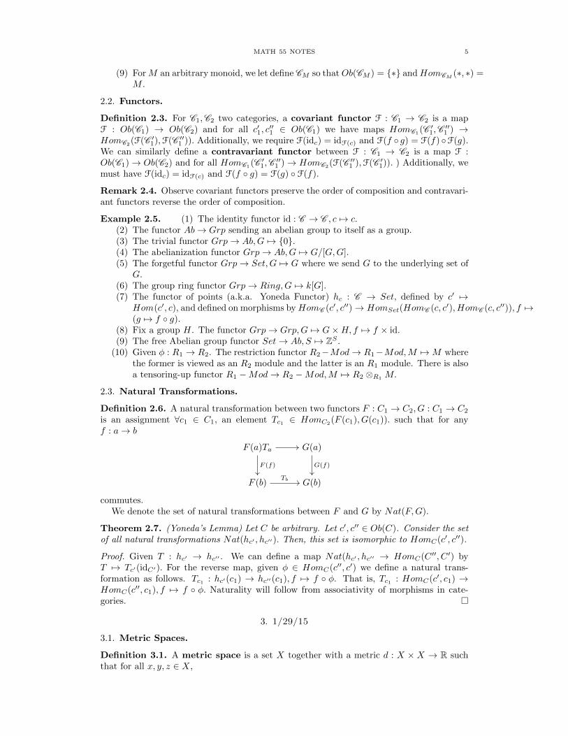
Definition 2.6. A natural transformation between two functors F : C1 → C2, G : C1 → C2
is an assignment ∀c1 ∈ C1, an element Tc1 ∈ HomC2(F (c1), G(c1)). such that for any
f : a→ b
F (a)Ta G(a)
F (b) G(b)
F (f) G(f)
Tb
commutes.We denote the set of natural transformations between F and G by Nat(F,G).
Theorem 2.7. (Yoneda’s Lemma) Let C be arbitrary. Let c′, c′′ ∈ Ob(C). Consider the setof all natural transformations Nat(hc′ , hc′′). Then, this set is isomorphic to HomC(c′, c′′).
Proof. Given T : hc′ → hc′′ . We can define a map Nat(hc′ , hc′′ → HomC(C ′′, C ′) byT 7→ Tc′(idC′). For the reverse map, given φ ∈ HomC(c′′, c′) we define a natural trans-formation as follows. Tc1 : hc′(c1) → hc′′(c1), f 7→ f φ. That is, Tc1 : HomC(c′, c1) →HomC(c′′, c1), f 7→ f φ. Naturality will follow from associativity of morphisms in cate-gories.
3. 1/29/15
3.1. Metric Spaces.
Definition 3.1. A metric space is a set X together with a metric d : X ×X → R suchthat for all x, y, z ∈ X,
6 AARON LANDESMAN
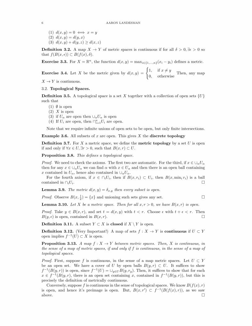
(1) d(x, y) = 0 ⇐⇒ x = y(2) d(x, y) = d(y, x)(3) d(x, y) + d(y, z) ≥ d(x, z)
Definition 3.2. A map X → Y of metric spaces is continuous if for all δ > 0,∃ε > 0 sothat f(B(x, ε)) ⊂ B(f(x), δ).
Exercise 3.3. For X = Rn, the function d(x, y) = maxi∈1,...,n(xi − yi) defines a metric.
Exercise 3.4. Let X be the metric given by d(x, y) =
1, if x 6= y
0, otherwiseThen, any map
X → Y is continuous.
3.2. Topological Spaces.
Definition 3.5. A topological space is a set X together with a collection of open sets Usuch that
(1) ∅ is open(2) X is open(3) if Uα are open then ∪αUα is open(4) If Ui are open, then ∩ni=1Ui are open.
Note that we require infinite unions of open sets to be open, but only finite intersections.
Example 3.6. All subsets of x are open. This gives X the discrete topology
Definition 3.7. For X a metric space, we define the metric topology by a set U is openif and only if ∀x ∈ U,∃r > 0, such that B(x, r) ⊂ U .
Proposition 3.8. This defines a topological space.
Proof. We need to check the axioms. The first two are automatic. For the third, if x ∈ ∪αUαthen for any x ∈ ∪αUα we can find α with x ∈ Uα and then there is an open ball containingx contained in Uα, hence also contained in ∪αUα.
For the fourth axiom, if x ∈ ∩iUi, then if B(x, ri) ⊂ Ui, then B(x,mini ri) is a ballcontained in ∩iUi.
Lemma 3.9. The metric d(x, y) = δx,y then every subset is open.
Proof. Observe B(x, 12 ) = x and unioning such sets gives any set.
Lemma 3.10. Let X be a metric space. Then for all x, r > 0, we have B(x, r) is open.
Proof. Take y ∈ B(x, r), and set t = d(x, y) with t < r. Choose ε with t + ε < r. ThenB(y, ε) is open, contained in B(x, r).
Definition 3.11. A subset Y ⊂ X is closed if X \ Y is open.
Definition 3.12. (Very Important!) A map of sets f : X → Y is continuous if U ⊂ Yopen implies f−1(U) ⊂ X is open.
Proposition 3.13. A map f : X → Y between metric spaces. Then, X is continuous, inthe sense of a map of metric spaces, if and only if f is continuous, in the sense of a map oftopological spaces.
Proof. First, suppose f is continuous, in the sense of a map metric spaces. Let U ⊂ Ybe an open set. We have a cover of U by open balls B(y, r) ⊂ U . It suffices to showf−1(B(y, r)) is open, since f−1(U) = ∪y∈UB(y, ry). Then, it suffices to show that for eachx ∈ f−1(B(y, r), there is an open set containing x, contained in f−1(B(y, r)), but this isprecisely the definition of metrically continuous.
Conversely, suppose f is continuous in the sense of topological spaces. We knowB(f(x), r)is open, and hence it’s preimage is open. But, B(x, r′) ⊂ f−1(B(f(x), r)), as we sawabove.
MATH 55 NOTES 7
3.3. The Intermediate Value Theorem.
Theorem 3.14. Let A ⊂ R be bounded above. Then, there exists a least upper bound. Thatis, there is y ∈ R with a ≤ y, but for any y′ < y, there is a ∈ A with a > y′.
Proof.
Remark 3.15. We can also take Theorem 3.14 as part of the definition of real numbers.
Theorem 3.16. Let f : [0, 1] → R be continuous. Say f(0) < 0, f(1) > 0. Then, thereexists a ∈ [0, 1] so that f(a) = 0.
Proof. Let A = x | f(x) < 0. Using Theorem 3.14, the set A has a least upper bound. Callit y. Then, we claim f(y) = 0. If f(y) < 0, using continuity, the preimage of V = [−∞, 0)is open, and since y lies in the preimage of V, there is an open set y ∈ U ⊂ f−1(U), with Uopen. In particular, taking a ∈ U, a > y, we obtain with a bigger than y, but a ∈ A. Thisis possible, as by metric continuity, we can take U to be an open ball. Hence, y is not anupper bound. The case f(y) > 0 is analogous, except in this case, we produce an upperbound for A less than y.
Remark 3.17. Note this is false if we replace R by Q. For instance, this fails for f(x) =
x+ 1−√
2.
4. 2/3/15
Review from last time:
(1) Metric Spaces(2) Topological Spaces(3) Metric Topology
Definition 4.1. A map X → Y is a homeomorphism if f is bijective and f, f−1 arecontinuous.
Remark 4.2. The notion of homeomorphism corresponds to isomorphism in the categoryof topological spaces.
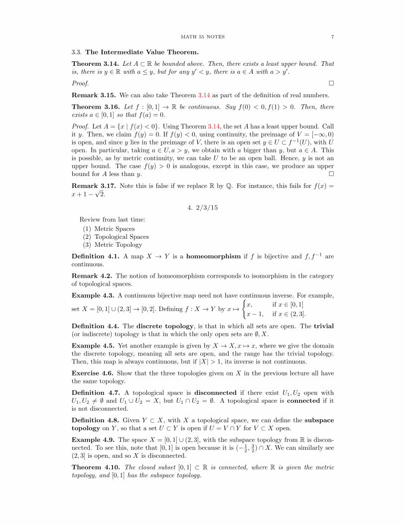
Example 4.3. A continuous bijective map need not have continuous inverse. For example,
set X = [0, 1] ∪ (2, 3]→ [0, 2]. Defining f : X → Y by x 7→
x, if x ∈ [0, 1]
x− 1, if x ∈ (2, 3].
Definition 4.4. The discrete topology, is that in which all sets are open. The trivial(or indiscrete) topology is that in which the only open sets are ∅, X.
Example 4.5. Yet another example is given by X → X,x 7→ x, where we give the domainthe discrete topology, meaning all sets are open, and the range has the trivial topology.Then, this map is always continuous, but if |X| > 1, its inverse is not continuous.
Exercise 4.6. Show that the three topologies given on X in the previous lecture all havethe same topology.
Definition 4.7. A topological space is disconnected if there exist U1, U2 open withU1, U2 6= ∅ and U1 ∪ U2 = X, but U1 ∩ U2 = ∅. A topological space is connected if itis not disconnected.
Definition 4.8. Given Y ⊂ X, with X a topological space, we can define the subspacetopology on Y , so that a set U ⊂ Y is open if U = V ∩ Y for V ⊂ X open.
Example 4.9. The space X = [0, 1] ∪ (2, 3], with the subspace topology from R is discon-nected. To see this, note that [0, 1] is open because it is (− 1
2 ,32 ) ∩X. We can similarly see
(2, 3] is open, and so X is disconnected.
Theorem 4.10. The closed subset [0, 1] ⊂ R is connected, where R is given the metrictopology, and [0, 1] has the subspace topology.
8 AARON LANDESMAN
Proof. Assume [0, 1] = U1 ∪U2 with U1 ∩U2 = ∅. We can assume 1 /∈ U1. Then, in fact theleast upper bound of U1 must be less than 1, because there is some open set containing 1,which is contained in U1. Let y = LUB(U1). We know y < 1.
There are now two cases: either y ∈ U1 or y 6 U1.Let us assume, for now y 6= 1. If y ∈ U1, then there exists r with (y − r, y + r) ⊂ U1¡
implying y + r2 ∈ U1. So, y + r
2 > y, implying y was not the upper bound of U1.If y /∈ U1, then y ∈ U2, and so there exists r so that (y − r, y + r) ⊂ U2, and we can take
y − r2 is also an upper bound for U1 implying y was not a least upper bound for U1.
Corollary 4.11. (Intermediate Value Theorem) Any f : [0, 1]→ R, continuous with f(0) <0, f(1) > 0, then there exists a ∈ [0, 1] with f(a) = 0
Proof. Let U1 = (−∞, 0), U2 = (0,∞), if there does not exist such an a, then f−1(U1) ∪f−1(U2) covers [0, 1], implying [0, 1] is disconnected, a contradiction.
Definition 4.12. A sequence (in X) is a map N → X. We often identify this functionwith the set of points in its image, indexed by natural numbers.
Definition 4.13. Let X be a topological space. A sequence of points xn → x if for allx ∈ U ⊂ X open, there exists N such that for all n ≥ N, xn ∈ U .
Example 4.14. If X has the trivial topology, then any sequence converges to all points ofX.
Definition 4.15. A topological space is Hausdorff if for any x′ 6= x′′ there are U ′, U ′′ withx′ ∈ U ′, x′′ ∈ U ′′ so that U ′ ∩ U ′′ 6= ∅.
Lemma 4.16. If X is a Hausdorff space (e.g. a metric space), and xn → x′, xn → x′′, thenx′ = x′′.
Proof. Suppose the sequence converges to two distinct points x′, x′′. If x′ ∈ U ′, x′′ ∈ U ′′ takeN ′, N ′′ as in the definition of convergence for x′, x′′. Then, n ≥ N ′ =⇒ xn ∈ U ′, n ≥ N ′′.Taking n ≥ max(N ′, N ′′) we obtain a contradiction, as xn ∈ U ′ ∩ U ′′ = ∅.
Lemma 4.17. Any Metric space X is Hausdorff.
Proof. For x, y ∈ X, say d(x, y) = r. Then, B(x, r/4), B(y, r/4) define two open setscontaining x, y which do not intersect.
Definition 4.18. Let X be a set. Define the cofinite topology on X, by letting all closedsets be those that are of the form
(1) ∅(2) X(3) x1, . . . , xn
Example 4.19. If X is an infinite set with the cofinite topology, then X is not Hausdorff.Indeed, U1 ∩ U2 6= ∅ if both U1 6= ∅, U2 6= ∅.
Theorem 4.20. Let xn = 1n . Then, xn → 0.
Proof. Given r, take N > 1r . Then, for all n ≥ N , we have xn = 1
n <1N ≤ r.
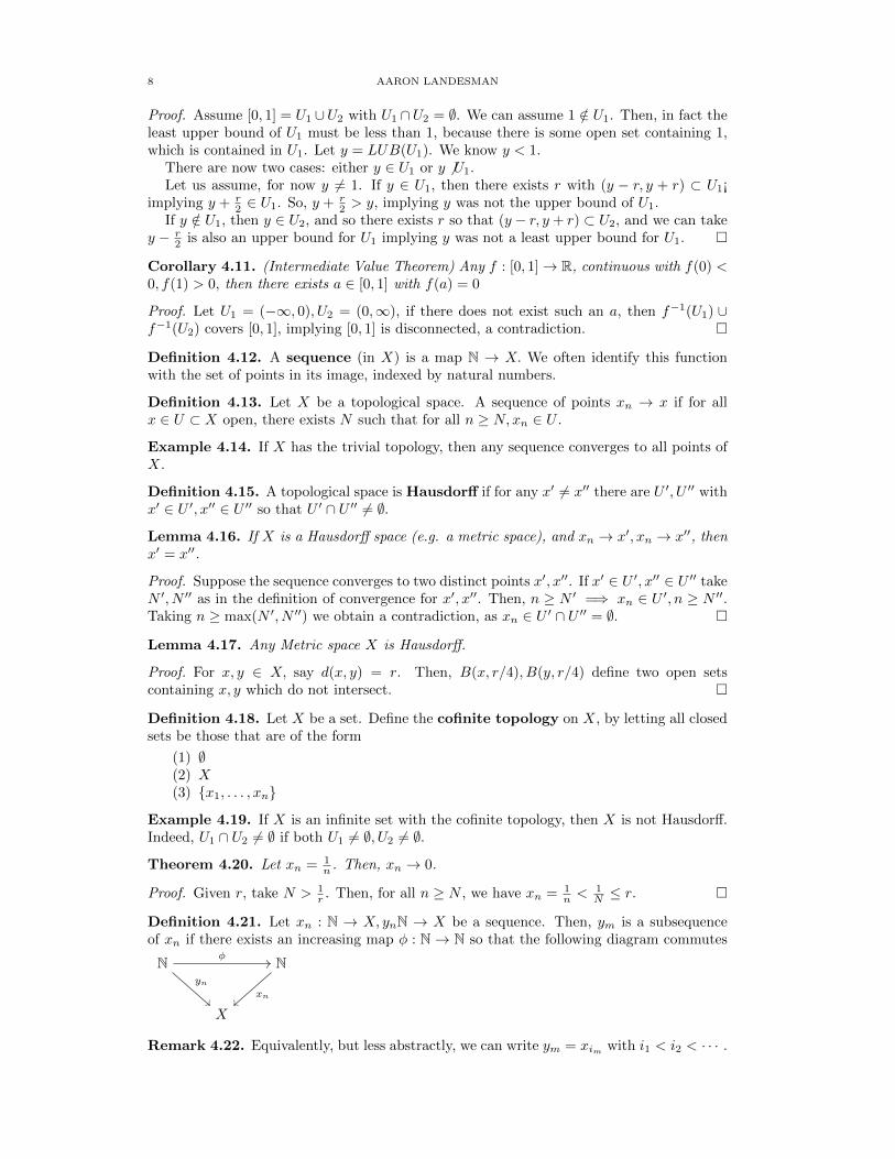
Definition 4.21. Let xn : N → X, ynN → X be a sequence. Then, ym is a subsequenceof xn if there exists an increasing map φ : N → N so that the following diagram commutes
N N
X
yn
φ
xn
Remark 4.22. Equivalently, but less abstractly, we can write ym = xim with i1 < i2 < · · · .
MATH 55 NOTES 9
Definition 4.23. Let xn be a sequence in X. Then, x is a partial limit of xn if there existsa subsequence xin that converges to x.
Lemma 4.24. Let xn be a sequence such that
(1) xn → x if and only if for all U, x ∈ U , then for all but finitely many n ∈ N, we haveXn ∈ U .
(2) Assuming further that X is a first countable space (e.g. a metric space), X is apartial limit if and only if for all r, there exist infinitely many n so that xn ∈ B(x, r).
Proof. (1) Pick an N so that for all n > N , xn in U . Then, there are only finitelymany xn /∈ U , namely, there are at most N such xi. Conversely, choose N to be themaximum over all N with xn /∈ U .
(2) Let x be a partial limit. We want to know that for all U , there are infinitely indicesi with xi ∈ U . Let xin be a convergent subsequence so that for all U , there existsN so that for all n ≥ N , we have xin ∈ U .
By first countability, we will construct a chain · · · ⊂ U4 ⊂ U3 ⊂ U2 ⊂ U1. Takexi1 ∈ U1. There exists i2 > i1 so that xi2 ∈ U2. This produces a subsequence xin sothat xin ∈ Un. Then, xin → x. To see this, for any U, x ∈ U , by first countability,we have some UN ⊂ U . Then xin ∈ UN for n ≥ N , hence xin ∈ U for n ≥ N . So, xis a partial limit of xn.
Definition 4.25. Let X be a metric space. Let xn be a sequence. Then, xn is Cauchy iffor all r there exists N so that for any n′, n′′ ≥ N , we have d(xn′ , xn′′) < r.
Definition 4.26. Let X be a metric space. A subset A ⊂ X is bounded if ∃x,R withA ⊂ B(x,R).
Lemma 4.27. (1) Every Cauchy sequence is bounded.(2) If a Cauchy sequence has a partial limit x then it converges to x.
Proof. (1) Take r = 1. There existsN so that for all n′, n′′ ≥ N we have d(xn′ , xn′′) < 1.So, choosing a large enough ball around xN , with radius bigger than 1, so that thefirst N terms lie in that ball, then all of the sequence will lie in that ball.
(2) Let xin → x. Pick r. We want and N so that for all n ≥ N , then xn ∈ B(x, r).Pick N given by the definition of Cauchy, so that for any n′, n′′ ≥ N , we haved(xn′ , xn′′) <
r2 . Then, there exists k > N , so that d(xik , x) < r/2. Then, d(x, xn) ≤
d(x, xk) + d(xk, xn) < r/2 + r/2 = r.
Definition 4.28. A space X is complete if every Cauchy sequence converges.
Lemma 4.29. If xn converges, then xn is Cauchy.
Proof. Follows from the triangle inequality.
Theorem 4.30. (Heine-Borel) Every bounded sequence in R has a partial limit.
Proof. Let
A = a ∈ R | there exist infinitely many indices n such that xn ≥ a.First, A 6= ∅ because xn is bounded from below. Second, A is bounded above, becausexn are bounded above. Let y = LUB(A). We will show that for all r there are infinitelymany n so that xn ∈ (y − r, y + r). Suppose not. Then, there are infinitely many n so thatxn ≥ y + r. Then, y + r/2 ∈ A, contradicting that y = LUB(A).
Suppose that all but finitely many xn are ≤ y− r. Then, y− r/2 would also be an upperbound for A, and so y is not the least upper bound.
Theorem 4.31. Every Cauchy sequence in R converges.
Proof. Every Cauchy sequence is bounded, as we saw above. If x is a partial limit of oursequence, then since our sequence is Cauchy, it actually converges to x.
10 AARON LANDESMAN
5. 2/5/15
Review:
(1) Cauchy sequences(2) Convergent =⇒ Cauchy Convergent(3) X is complete if every Cauchy sequence is convergent(4) R is complete(5) (Weierstrass) every sequence in [0, 1] has a convergent subsequence.
Definition 5.1. A subset X ′ ⊂ X is dense if for any U ⊂ X,X ′ ∩ U 6= ∅.
Lemma 5.2. If X is a metric space, X ′ ⊂ X is dense if and only if for all x, r thenB(x, r) ∩X ′ 6= ∅.
Proof. If X ′ is dense, then we know it intersects every open set, in particular it intersects anyball. Conversely, if X ′ intersects every ball non-trivially, we know every open set contains aball, so it intersects every open set non-trivially.
Theorem 5.3. Let X be a metric space.
(1) There exists i : X → X so that(a) X is complete(b) i is an isometric embedding(c) Im(i) is dense.
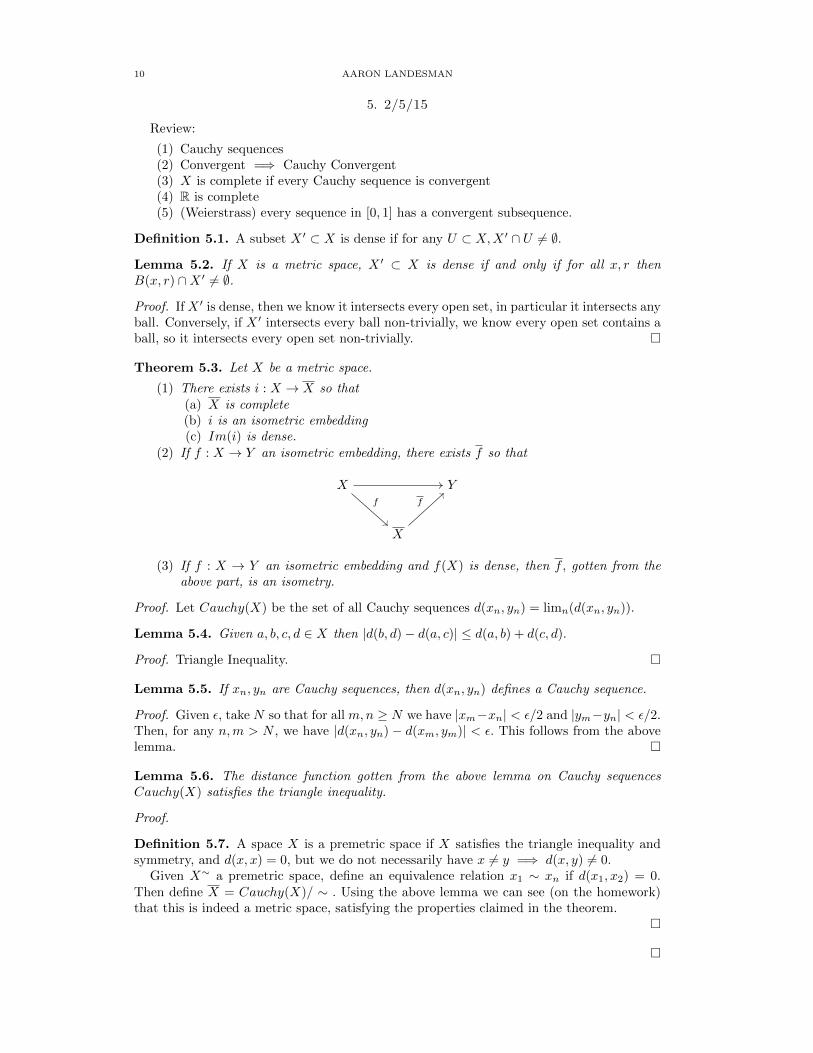
(2) If f : X → Y an isometric embedding, there exists f so that
X Y
X
f f
(3) If f : X → Y an isometric embedding and f(X) is dense, then f, gotten from theabove part, is an isometry.
Proof. Let Cauchy(X) be the set of all Cauchy sequences d(xn, yn) = limn(d(xn, yn)).
Lemma 5.4. Given a, b, c, d ∈ X then |d(b, d)− d(a, c)| ≤ d(a, b) + d(c, d).
Proof. Triangle Inequality.
Lemma 5.5. If xn, yn are Cauchy sequences, then d(xn, yn) defines a Cauchy sequence.
Proof. Given ε, take N so that for all m,n ≥ N we have |xm−xn| < ε/2 and |ym−yn| < ε/2.Then, for any n,m > N , we have |d(xn, yn) − d(xm, ym)| < ε. This follows from the abovelemma.
Lemma 5.6. The distance function gotten from the above lemma on Cauchy sequencesCauchy(X) satisfies the triangle inequality.
Proof.
Definition 5.7. A space X is a premetric space if X satisfies the triangle inequality andsymmetry, and d(x, x) = 0, but we do not necessarily have x 6= y =⇒ d(x, y) 6= 0.
Given X∼ a premetric space, define an equivalence relation x1 ∼ xn if d(x1, x2) = 0.Then define X = Cauchy(X)/ ∼ . Using the above lemma we can see (on the homework)that this is indeed a metric space, satisfying the properties claimed in the theorem.
MATH 55 NOTES 11
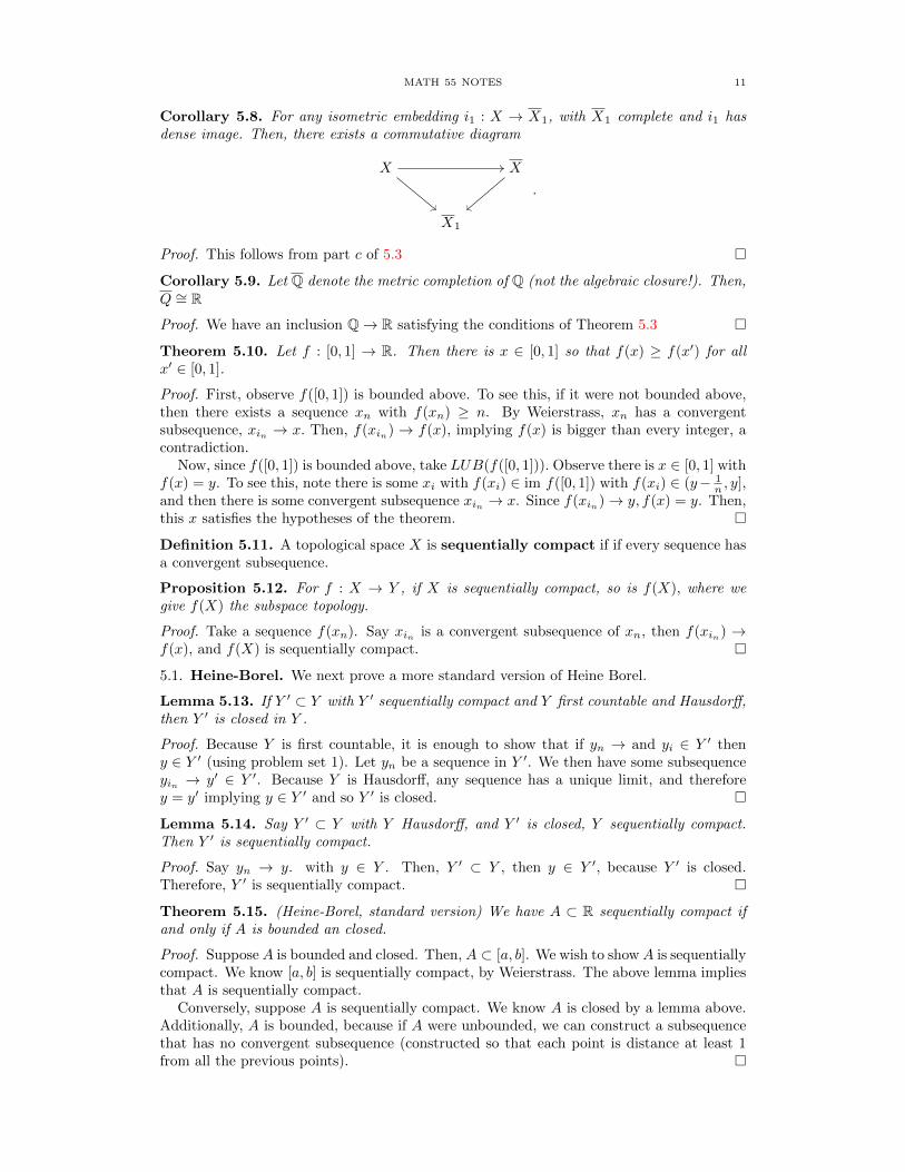
Corollary 5.8. For any isometric embedding i1 : X → X1, with X1 complete and i1 hasdense image. Then, there exists a commutative diagram
X X
X1
.
Proof. This follows from part c of 5.3
Corollary 5.9. Let Q denote the metric completion of Q (not the algebraic closure!). Then,Q ∼= R
Proof. We have an inclusion Q→ R satisfying the conditions of Theorem 5.3
Theorem 5.10. Let f : [0, 1] → R. Then there is x ∈ [0, 1] so that f(x) ≥ f(x′) for allx′ ∈ [0, 1].
Proof. First, observe f([0, 1]) is bounded above. To see this, if it were not bounded above,then there exists a sequence xn with f(xn) ≥ n. By Weierstrass, xn has a convergentsubsequence, xin → x. Then, f(xin) → f(x), implying f(x) is bigger than every integer, acontradiction.
Now, since f([0, 1]) is bounded above, take LUB(f([0, 1])). Observe there is x ∈ [0, 1] withf(x) = y. To see this, note there is some xi with f(xi) ∈ im f([0, 1]) with f(xi) ∈ (y− 1
n , y],and then there is some convergent subsequence xin → x. Since f(xin)→ y, f(x) = y. Then,this x satisfies the hypotheses of the theorem.
Definition 5.11. A topological space X is sequentially compact if if every sequence hasa convergent subsequence.
Proposition 5.12. For f : X → Y , if X is sequentially compact, so is f(X), where wegive f(X) the subspace topology.
Proof. Take a sequence f(xn). Say xin is a convergent subsequence of xn, then f(xin) →f(x), and f(X) is sequentially compact.
5.1. Heine-Borel. We next prove a more standard version of Heine Borel.
Lemma 5.13. If Y ′ ⊂ Y with Y ′ sequentially compact and Y first countable and Hausdorff,then Y ′ is closed in Y .
Proof. Because Y is first countable, it is enough to show that if yn → and yi ∈ Y ′ theny ∈ Y ′ (using problem set 1). Let yn be a sequence in Y ′. We then have some subsequenceyin → y′ ∈ Y ′. Because Y is Hausdorff, any sequence has a unique limit, and thereforey = y′ implying y ∈ Y ′ and so Y ′ is closed.
Lemma 5.14. Say Y ′ ⊂ Y with Y Hausdorff, and Y ′ is closed, Y sequentially compact.Then Y ′ is sequentially compact.
Proof. Say yn → y. with y ∈ Y . Then, Y ′ ⊂ Y , then y ∈ Y ′, because Y ′ is closed.Therefore, Y ′ is sequentially compact.
Theorem 5.15. (Heine-Borel, standard version) We have A ⊂ R sequentially compact ifand only if A is bounded an closed.
Proof. SupposeA is bounded and closed. Then, A ⊂ [a, b]. We wish to show A is sequentiallycompact. We know [a, b] is sequentially compact, by Weierstrass. The above lemma impliesthat A is sequentially compact.
Conversely, suppose A is sequentially compact. We know A is closed by a lemma above.Additionally, A is bounded, because if A were unbounded, we can construct a subsequencethat has no convergent subsequence (constructed so that each point is distance at least 1from all the previous points).
12 AARON LANDESMAN
Lemma 5.16. If A ⊂ R is bounded and closed, then LUB(A) ∈ A
Proof. Done above in the proof of completions.
Lemma 5.17. Heine-Borel implies Theorem 5.10
Proof. We know [0, 1] is bounded and closed, so [0, 1], is sequentially compact, so f([0, 1])is sequentially compact, hence bounded and closed, by Heine-Borel.
Definition 5.18. (Important Definition!) A topological space is compact if ∪α∈AUα = Xthen there is a finite subset A′ ⊂ A so that ∪α∈A′Uα = X.
Proposition 5.19. If f : X → Y is continuous and X compact, then f(X) is compact.
Proof. Choose an open cover f(X) = ∪αUα. Then, ∪αf−1(Uα) = X. Choose a finite subsetB ⊂ A. Then, ∪βf−1(Uβ) = X implies ∪βUβ = f(X).
Lemma 5.20. Y ′ ⊂ Y with Y ′ compact (in the subset topology) and Y Hausdorff, then Y ′
is closed.
Proof. It suffices to show U = Y \ Y ′ is open. For this, it suffices to show each x ∈ Y , wehave some open set V with x ∈ V ⊂ U . To do this, for each y ∈ Y ′, take Ay, By opensets with y ∈ Ay, x ∈ By and Ay ∩ By = ∅, which exist as Y is Hausdorff. Therefore,∪y∈YAy. By compactness of Y ′, we have a finite subset y1, . . . , yn so that Y ⊂ ∪ni=1Ayi .Therefore, V = ∩ni=1Byi ⊂ U , which is a finite intersection of opens, hence open. It followsthat x ∈ V ⊂ U is an open set of the desired form. Hence, U is open, and Y ′ is closed.
Definition 5.21. We say X is first countable if every x ∈ X has a countable neighborhoodbase. That is, there exist countably many U1, . . . , Un, . . . so that for every open x ∈ U thereis some Ui with Ui ⊂ U .
Proposition 5.22. Say X is first countable and compact. Then X is sequentially compact.
Proof. Say xn is a sequence. Suppose it has no partial limits. For every x ∈ X thereis Ux ⊂ X with Ux contains only finitely may xi in the sequence. Then, ∪xUx = X. Bycompactness, there exists a finite cover ∪ni=1Uxi = X. But this only contains a finite numberof elements of our sequence, implying the entire space has only finitely many elements ofthe sequence, a contradiction.
Definition 5.23. A neighborhood base for a topological space X is a collection of opensets of X,Ui so that any open set U in X can be written as U = ∪iUi.
Definition 5.24. A space X is second countable if if has a countable neighborhood base.That is, a neighborhood base containing only countable many closed subsets.
Proposition 5.25. If X is second countable, and sequentially compact, then X is compact.
Proof.
6. 2/12/15
Lemma 6.1. (1) If ai → a, bi → b then if we define ci = ai + bi then ci → a+ b.(2) aibi → ab(3) For a 6= 0, we have 1/ai → 1/a.
Proof. This follows from continuity of addition multiplication, and inversion, which can bechecked by simple ε, δ arguments.
Lemma 6.2. (Sandwich Rule) If a′n ≤ an ≤ a′′n and a′n → a, a′′n → a then an → a.
Proof. Use ε, δ arguments.
Example 6.3. For |a| < 1 we have an → 0. To see this, write b = 1a and then bn =
(1 + (b− 1))n ≥ n(b− 1). Then, 0 ≤ an ≤ 1(b−1)n and by the sandwich rule, an → 0.
MATH 55 NOTES 13
Lemma 6.4. For any a ∈ R ≥ 0, a1n exists.
Proof. Intermediate value theorem, applied to f(x) = xn.
Example 6.5. We have a1n → 1 as n → ∞. To see this, it suffices to show it for a > 1,
using the fact that 1ai→ 1 implies ai → 1. Then, 1 ≤ a
1a ≤ 1 + a−1
n , using the binomialtheorem.
Example 6.6. We have n1n → 1. We can again use the sandwich rule, bounding 1 ≤ n 1
n ≤2
n−1 , again using the binomial theorem, since (1 + (n1n − 1))n ≥ n(n− 1)(n
1n − 1)/2.
Definition 6.7. Given ai a sequence the series ai refers to the partial sums bi =∑ni=1 ai.
Notation 6.8. From now on, we will often use ai to denote a series, and bi to denote the
corresponding partials sums bi =∑ij=1 aj .
Definition 6.9. Let ai be a series with∑ni=1 ai = bi. Then we say the series ai converges
if the sequence bi converges.
Definition 6.10. The series ai converges absolutely if the series |ai| converges.
Lemma 6.11. Let an = an for |a| < 1. This series converges absolutely.
Proof. We have∑i ai = 1
1−a −1
1−aan+1 → 1
a−1 .
Lemma 6.12. If the series an converges then the sequence an converges to 0.
Proof. Say bn → a and bn+1 → a then ai = bn+1 − bn → a− a = 0.
Lemma 6.13. The series an converges if and only if for every ε > 0 there exists N so that|∑n2
i=n1ai| < ε
Proof. This condition is equivalent to the sequence bi of partial sums being Cauchy. But,since the reals are complete, Cauchy convergence is equivalent to convergence.
Lemma 6.14. If ai converges absolutely, then it converges.
Proof. We have |∑n2
i=n1|ai|| ≤ ε then certainly |
∑n2
i=n1ai| ≤ ε by the triangle inequality,
and this implies convergence by the previous lemma.
Theorem 6.15. Let an converge absolutely. and φ : N → N, then aφ(i) converges and thesum equals
∑i ai.
Proof.
Theorem 6.16. Let an be convergent but not absolutely convergent. Then, for any b ∈ R,there exists φ : N→ N with
∑i aφ(i) = b.
Proof. Omitted, see Rudin.
Example 6.17. A sequence which converges but not absolutely is ai =
1/√i/2, if n ≡ 0 (mod 2)
−1/√
(i− 1)/2 otherwise
Lemma 6.18. Let bn be a bounded, monotonically increasing sequence. Then bn is conver-gent.
Proof. (Sketch) Let B = lim sup bi, which exists as bi is bounded. We claim bi → B. To seethis, take any ε > 0 and then there exists some N so that for any n > N we have bn > B−r.Since B is an upper bound, and bi are arbitrarily close to B, we have bi → B.
Proposition 6.19. Let an have positive terms. Then, an converges if and only if thereexists A > 0 so that
∑i ai ≤ A.
Proof. If the partial sums converge to b, then b bounds bn for all n. For the converse, usethe above lemma.
14 AARON LANDESMAN
Corollary 6.20. Say ai, ai have positive terms. If∑ni=1 ai ≤
∑ni=1 ai for all n and ai
converges then ai converges.
Proof.
Proposition 6.21. (1) Let ai be so that lim sup n√|an| < 1 =⇒ an converges abso-
lutely.(2) Let an be so that lim sup |an|
1n > 1 then an diverges.
Proof. (1) Let a = lim sup |an|1n . Take a = lim sup |an|
1n and ai = ai. For all but
finitely many i, we have |ai|1n ≤ a if and only if |ai| ≤ ai, and we know ai converges
as it is a geometric series.(2) We have the ai do not converge to 0, as there are infinitely many i for which |ai| ≥ 1.
Proposition 6.22. Assume that lim sup |ai+1
ai| < 1. Then, ai converge absolutely.
Proof. Let r = lim sup |an+1
an| and for all but finitely many i we have |ai+1
ai| and so we may
take r ≤ r′ < 1 we may assume ai+1
ai< r′ and so ai+1 ≤ r′i|a1|.
Example 6.23. Let an = xn
n! . This converges absolutely. Note an+1
an= x/n + 1 → 0. It
satisfies the ratio test, and hence converges.
Example 6.24. Take an = 1na for a > 0. Then, if we use the ration test, we have an+1
an→ 1.
The root test also is inconclusive, since 1
nan→ 1.
Lemma 6.25. Let an be a series of positive numbers that is monotonically decreasing, andlet an = 2na2n . Then an converges if and only if an does.
Proof. Homework.
Theorem 6.26. The series 1na converges for a > 1 and diverges for a ≤ 1.
Proof. For our series, using the associated zeta series from the above lemma an = 12(a−1)n =
1bn , which converges if and only if b > 1, which is equivalent to a > 1.
Definition 6.27. Let exp(x) =∑∞i=0
xi
i!
Lemma 6.28. If an converge absolutely to A and bn converge absolutely to B and cn =∑i aibn−i then cn converges absolutely and converges to AB
Proof. We want to find and N for which∑2Ni=0 ci−AB) < ε. Consider |(
∑ni=0 an)·(
∑ni=0 bn−
AB| < ε3 for n ≥ N . These two sums differ by a sum of aibj with i + j ≤ 2n but i > n or
j > n. Then,
|∑
j≤n,n≤i≤2n
aibj | <∑
1≤j≤n
bj ·∑
n<i≤2n
|ai| < B ·∑
n<i≤2n
ai < B · ε/B = ε,
where the penultimate step uses cauchyness of bi.
Theorem 6.29. exp(x) exp(y) = exp(x+ y).
Proof. Note (x+y)n
n! =∑ni=0
xiyn−i
i!(n−i)! , and so we can use the above lemma.
Definition 6.30. Let X be a sequentially compact topological space. Let Functcont(X,Y )denote the set of continuous functions f : X → Y .
Define a metric on Functcont(X,R) by ρ(f, g) = maxx∈X |f(x)− g(x)|.
Lemma 6.31. The function ρ defined above is a metric.
Proof. Omitted.
Definition 6.32. Let f : X → Y be a map between metric spaces. We say f is uniformlycontinuous if for all ε there exists δ such that ρ(x1, x2) < δ, then ρ(f(x1), f(x2)) < ε.
MATH 55 NOTES 15
Example 6.33. If ρ(f(x1), f(x2)) ≤ C · ρ(x1, x2) then f is uniformly continuous. Suchfunctions are called lipschitz functions.
Proposition 6.34.
X ′ X
Y
f ′
i
with X ′ → X a dense injection, f ′ uniformly continuous, Y complete. Then, there existsf : X → Y so that f ′ = f i and f uniformly continuous.
Proof. Given x ∈ X choose xn → x, with xn ∈ X ′.
Lemma 6.35. We have f(xn) is convergent.
Proof. We see xn is Cauchy. By uniform continuity, f(xn) is Cauchy. As Y is complete,f(xn)→ y.
Define y = limn f(xn), and define f(x) = y. We only need show f is uniformly continuous.Given ε, let δ be so that ρ(x1, x2) < δ =⇒ ρ(f(x1), f(x2)) < ε for x1, x2 ∈ X ′. We wantthe same for x1, x2 ∈ X. Take x1, x2 ∈ X let ρ(x1, x2) = δ′ < δ. We want to showρ(f(x1), f(x2)) < ε. Choose xn1 → x1, x
n2 → x2. So, for n > N , we have ρ(xn1 , x
n2 ) < δ. So,
ρ(f(x1), f(x2)) = limn ρ(f(xn1 ), f(xn2 )). Therefore, rho(f(x1), f(x2)) ≤ ε.Uniqueness follows from the fact that Y is Hausdorff, so the sequence converges to a
unique limit point.
Definition 6.36. Define Functcont,pw−linear(X,R) to be the set of continuous piecewiselinear functions f : X → R.
Corollary 6.37. Given
Functcont([a, b],R) R
Functcont,pw−linear([a, b],R)
∫
we get a unique map∫
: Functcont([a, b],R)→ R.
Proof. We need to check uniform continuous of∫
. If maxx |f(x) − g(x)| < C then |∫f −∫
g| ≤ (b− a)C then |∫f −
∫g| ≤ (b− a) maxx(|f(x)− g(x)|). If f is piecewise linear, then
|f | < C implies |∫f | < (b− a)C.
Theorem 6.38. We have Functcont,pw−linear([a, b],R) is dense in Functcont([a, b],R).
Proof. Let us prove this, assuming Theorem 6.39 below. But this is immediate, as [a, b] is
compact. Given f : [a, b] → R, and ε we will produce f piecewise linear so that ρ(f(x) −f(x)| < ε. Choose the δ given by uniform continuity. Choose a partition of [a, b] into
[xi, xi+1] with |xi−xi+1| < δ. Then, define f(x) = f(xi), for xi ≤ x < xi+1. It is then clearthat
Theorem 6.39. Let X be a compact metric space and f : X → Y . Then f continuousimplies f is uniformly continuous.
Proof. Given ε we want δ so that ρ(x1, x2) < δ implies f(x1, x2) < ε.
Proof 1. For all x let δx be so that ρ(x′, x) < δx implies ρ(f(x), f(x′)) < ε/2. Considerthe balls B(x, δx). Let X = ∪xB(x, δx/2). We can replace this by a finite subcover, andlet δ = min(δx/2). We claim this δ works, because ρ(x1, x2) < δimplies there exists x withx1, x2 ∈ B(x, δx) implies ρ(f(x1), f(x)) < ε/2, ρ(f(x2), f(x)) < ε/2 =⇒ ρ(f(x1), f(x2)) <ε.
16 AARON LANDESMAN
Proof 2. For all n, there exists xn1 , xn2 so that ρ(xn1 , x
n2 ) < 1/n but ρ(f(x1), f(x2)) ≥ ε.
Choose convergent subsequences of xni → xi, and we obtain x1 = x2 = x. This is acontradiction, as for N large enough, we have ρ(f(x)−f(xni )) < ε/3 implying ρ(f(x1, x2)) <ε.
Definition 6.40. We define a map∫: Functcont([a, b],R),
called integration by first defining it on linear functions, then continuous piecewise linearfunctions, then positive continuous functions, then all continuous functions.
(1) If f is linear on [a, b] then∫[a,b]
f = (b− a)d+b2 − a2
2c.
(2) If f is linear of [x0, x1], . . . , [xn−1, xn], with x0 = a, xn = b. The define∫[a,b]
f =
n∑i=1
∫[xi−1,xi]
f.
(3) For positive functions, define the integral by the extension of piecewise linear inte-grals, using the theorems above.
(4) For general functions f let f+ =∫
max(f, 0), f− =∫
min(0, f) and define∫f =∫
f+ +∫f−.
Lemma 6.41. (1)∫f1 + f2 =
∫f1 + f2.
(2)∫cf = c
∫f .
(3)∫
[a,b]−∫
[a,c]f +
∫[c,b]
f
(4) f ≥ 0 =⇒∫f ≥ 0.
(5) If f ≥ 0 and∫f = 0 then f = 0.
Proof. (1) Look at
Functcont,pw−linear([a, b],R)2 R
Functcont([a, b],R)2
and consider the two functions f1, f2 →∫f1 + f2 and f1, f2 7→
∫f1 +
∫f2.
(2) Consider
Functcont,pw−linear([a, b],R) R
Functcont([a, b],R)
The two functions f 7→ c·∫f, f 7→
∫cf obviously agree of piecewise linear functions,
hence everywhere.(3) Similar to the above part.(4)
Lemma 6.42. We have Functcont,pw−linear([a, b],R≥0) is dense in Functcont([a, b],R).
MATH 55 NOTES 17
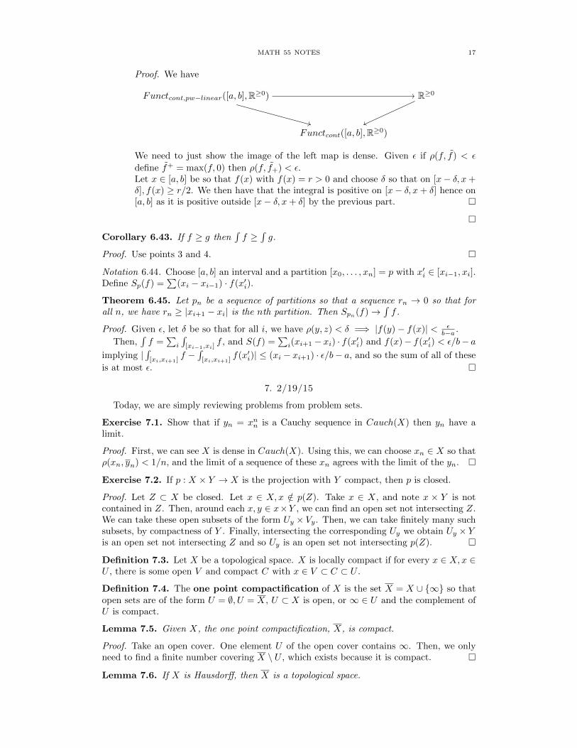
Proof. We have
Functcont,pw−linear([a, b],R≥0) R≥0
Functcont([a, b],R≥0)
We need to just show the image of the left map is dense. Given ε if ρ(f, f) < ε
define f+ = max(f, 0) then ρ(f, f+) < ε.Let x ∈ [a, b] be so that f(x) with f(x) = r > 0 and choose δ so that on [x− δ, x+δ], f(x) ≥ r/2. We then have that the integral is positive on [x− δ, x+ δ] hence on[a, b] as it is positive outside [x− δ, x+ δ] by the previous part.
Corollary 6.43. If f ≥ g then∫f ≥
∫g.
Proof. Use points 3 and 4.
Notation 6.44. Choose [a, b] an interval and a partition [x0, . . . , xn] = p with x′i ∈ [xi−1, xi].Define Sp(f) =
∑(xi − xi−1) · f(x′i).
Theorem 6.45. Let pn be a sequence of partitions so that a sequence rn → 0 so that forall n, we have rn ≥ |xi+1 − xi| is the nth partition. Then Spn(f)→
∫f .
Proof. Given ε, let δ be so that for all i, we have ρ(y, z) < δ =⇒ |f(y)− f(x)| < εb−a .
Then,∫f =
∑i
∫[xi−1,xi]
f , and S(f) =∑i(xi+1 − xi) · f(x′i) and f(x)− f(x′i) < ε/b− a
implying |∫
[xi,xi+1]f −
∫[xi,xi+1]
f(x′i)| ≤ (xi − xi+1) · ε/b− a, and so the sum of all of these
is at most ε.
7. 2/19/15
Today, we are simply reviewing problems from problem sets.
Exercise 7.1. Show that if yn = xnn is a Cauchy sequence in Cauch(X) then yn have alimit.
Proof. First, we can see X is dense in Cauch(X). Using this, we can choose xn ∈ X so thatρ(xn, yn) < 1/n, and the limit of a sequence of these xn agrees with the limit of the yn.
Exercise 7.2. If p : X × Y → X is the projection with Y compact, then p is closed.
Proof. Let Z ⊂ X be closed. Let x ∈ X,x /∈ p(Z). Take x ∈ X, and note x × Y is notcontained in Z. Then, around each x, y ∈ x×Y , we can find an open set not intersecting Z.We can take these open subsets of the form Uy × Vy. Then, we can take finitely many suchsubsets, by compactness of Y . Finally, intersecting the corresponding Uy we obtain Uy × Yis an open set not intersecting Z and so Uy is an open set not intersecting p(Z).
Definition 7.3. Let X be a topological space. X is locally compact if for every x ∈ X,x ∈U , there is some open V and compact C with x ∈ V ⊂ C ⊂ U .
Definition 7.4. The one point compactification of X is the set X = X ∪ ∞ so thatopen sets are of the form U = ∅, U = X, U ⊂ X is open, or ∞ ∈ U and the complement ofU is compact.
Lemma 7.5. Given X, the one point compactification, X, is compact.
Proof. Take an open cover. One element U of the open cover contains ∞. Then, we onlyneed to find a finite number covering X \ U , which exists because it is compact.
Lemma 7.6. If X is Hausdorff, then X is a topological space.
18 AARON LANDESMAN
Proof. It is straightforward to check that arbitrary unions of opens and finite intersectionsare open.
Lemma 7.7. We have X is Hausdorff if and only if X is locally compact.
Proof. Again, follows from the definitions.
Exercise 7.8. For r ∈ R the function xr exists.
Proof. Say rn → r. We want to show xrn is Cauchy.
Lemma 7.9. For x > 0, xr is monotonic.
Lemma 7.10. x1n → 1 as n→∞.
Then, xrn − xrm = xrn(xrm−rn − 1)→ 0.
Exercise 7.11. Show, xr is continuous.
Proof. If xi → x then xri − xr = xr((xi/x)r − 1). Since(xix
)ris monotonic in r so this ratio
converges to 0 as xi → x.
Exercise 7.12. Show ax is continuous in x.
Proof. It suffices to show ari → 1 as ri → 0, which follows as a1n → 1 and the squeeze
theorem.
Lemma 7.13. If f : [a, b]→ R is continuous and strictly increasing on rationals, then it ismonotonic on all reals.
Proof. For x < y, want f(x) < f(y). Just write both real numbers as a limit of rationals.
Lemma 7.14. The function ax is surjective onto R>0.
Proof. This follows from the intermediate value theorem.
8. 2/24/15
Definition 8.1. A function f : X → Y is continuous at x if for all f(x) ∈ Uy there existsx ∈ Ux with f(Ux) ⊂ UY .
Definition 8.2. A function f : X − x → Y , we say the limit of f at x is y if f can beextended to f : X → Y so that f(x) = y and f is continuous at x.
Lemma 8.3. The limit of f at x is y if for all Uy 3 y there exists Ux 3 x so that for allx′ ∈ Ux − x we have f(x′) 3 Uy.
Proof.
Remark 8.4. Let Y = R. If limx′→x fi(x′) = yi and limx′→x f1(x′)f2(x′) = y1y2, limx′→x f1(x′)+
f2(x′) = y1 + y2.If limx′→x f(x′) = 0 and g is bounded in X − x then limx′→x f(x′)g(x′) = 0.
Definition 8.5. Let X be a metric space and f : X − x0 → R. Then, f is o(ρ(x, x0)n), or
equivalently f ∈ o(ρ(x, x0)n), viewing o(ρ(x, x0)n) as a set of functions, if limx→x0
fρ(x,x0)n =
0 if and only if for all ε the is some δ so that ρ(x, x0) < δ implies f(x)| < ε|ρ(x, x0)|n.
Remark 8.6. Observe f is o(1) if and only if limx0→x f(x) = 0.
Example 8.7. If X = R and f(x) = x, x0 = 0. Then, for which n is f in o((x − x0)n)?Answer: only n = 0.
MATH 55 NOTES 19
Definition 8.8. We say f : [a, b]→ R is differentiable at x0 if there exists f ′(x0) ∈ R sothat f(x)− f(x0)− (x− x0)f ′(x0) is o(x− x0). I.e., if
limx→x0
f(x)− f(x0)− (x− x0)f ′(x0)
x− x0= 0.
Equivalently, for every ε there exists δ so that |x− x0| < δ implies
|f(x)− f(x0)− (x− x0)f ′(x0)
x− x0| < ε.
Lemma 8.9. If f ′(x0) exists, then it is unique.
Proof. Take the difference of two such derivatives, which is f ′1(x0)− f ′2(x0), but tends to 0,hence equals 0.
Lemma 8.10. If f is differentiable at x0 it is continuous at x0.
Proof. We want to see limx→x0f(x) = f(x0). Observe
limx→x0
f(x) = limx→x0
(f(x)− f(x0)− f ′(x0)(x− x0)
x− x0
)(x−x0)+f(x0)+f ′(x0)(x−x0) = f(x0).
Example 8.11. Say f(x) = x. What is f ′(x)? We see f ′(x0) = 1, directly from thedefinition.
Lemma 8.12. If f, g are differentiable at x0 then f ·g is differentiable at x0 and (f ·g)′(x0) =f ′(x0)g(x0) + f(x0)g′(x0).
Proof. Behold
limf(x)g(x)− f(x0)g(x0)− f ′(x0)g(x0) · (x− x0)− g′(x0)f(x0)(x− x0)
x− x0
= limf(x)g(x)− f(x0)g(x)− (x− x0)f ′(x0)g(x)
x− x0+f(x0)g(x)− f(x0)g(x)− (x− x0)g′(x0)f(x0)
x− x0+
(x− x0)g(x)− g(x0)f ′(x0)
x− x0
and all three terms tend to 0.
Example 8.13. We have f(x) = xn then f ′(x) = nxn−1.
Lemma 8.14. (Chain rule) Suppose f : (a, b)→ (c, d), g : (c, d)→ R. If f is differentiableat x0 and g at y0 = f(x0) then g f is differentiable at x0 and (g f)′(x0) = g′(y0) · f ′(x0).
Proof. Behold
limg f(x)− g f(x0)− g′(y0)f ′(x0)(x− x0)
x− x0
= limg(f(x))− g(y0)− g′(y0)f(x)− y0)
x− x0+g′(y0)(f(x)− y0 − g′(x0)(x− x0)
x− x0
= limg(f(x))− g(y0)− g′(y0)f(x)− y0)
x− x0
Now, we claim this goes to 0. First, for ε given, choose µ so that |y−y0| < µ implies |y−y0| <µ implies | g(y)−g′(y0)−g′(y0)(y−y0)
y−y0 | < ε. Let δ be so that |x − x0| < δ =⇒ |f(x) − y0| < µ,
and theng(f(x))− g(y0)− g′(y0)(f(x)− y0)
x− x0≤ εf(x)− y0
x− x0.
Note that lim f(x)−y0x−x0
= f ′(x0), is bounded, hence the above expression goes to 0.
20 AARON LANDESMAN
Theorem 8.15. Let f : [a, b] → R and f continuous on [a, b] is differentiable on (a, b).Then f attains its maximum at x0 ∈ (a, b) implies f ′(x0) = 0.
Proof. Assume f ′(x0) > 0. Then, f(x) = f(x0) + (x−x0)(f ′(x0) + f(x)−f(x0)−f ′(x0)(x−x0)x−x0
),
and so for x > x0 we have f(x) > f(x0).
Theorem 8.16. Let f : [a, b] → R be continuous and differentiable on (a, b) with f(a) =f(b). Then, there exists x ∈ (a, b) so that f ′(x) = 0.
Proof. Let x be the maximum point. The only problem is if the maximum occurs at one ofthe endpoints. Then let x be the minimum point. If that is also at one of the endpoints,the the function is constant.
Theorem 8.17. There exists x so that f(b)−f(a)b−a = f ′(x). Consider g(x) = f(x)− f(b)−f(a)
b−a (x−a). Then there is an x for which g′(x) = 0 and so g′(x) = f ′(x)− f(b)−f(a)
b−a .
Proof. (1) If f is differentiable on (a, b) then f ′(x) ≥ 0 implies f is nondecreasing(2) f ′(x) ≤ 0 implies f is non-increasing(3) f ′(x) = 0 implies f is constant.
(1) Suppose not. Then there exists x, y with x < y but f(x) > f(y). Then f(y)−f(x)y−x =
f ′(z), a contradiction.(2) Similar to the above(3) If f is not increasing and not decreasing, then f is constant.
Definition 8.18. Let f : (a, b) → R. We say that f is differentiable n times at X0 if f isdifferentiable n− 1 times on (a′, b′) 3 x0 and f (n−1) : (a′, b′)→ R is differentiable at x0.
Theorem 8.19. Let f be differentiable n times at x0 so that f (k)(x0) = 0 for k = 0, . . . , n.Then, f = o((x− x0)n).
Proof. If n = 1 we have f(x)x−x0
→ 0 is equivalent to f ∈ o((x − x0)n). Next, we will do
n = 2 as the general case is similar. Take f(x) = (x− x0)f ′(x1), we have f(x)/(x− x0)2 =f ′(x1)/(x− x0) ≤ f ′(x1)/(x1 − x0)→ 0.
For the n = 3 case,
f(x)
(x− x0)3=
f ′(x1)
(x− x0)2≤ f ′(x1)
(x− x0)(x1 − x0)≤ f ′′(x0)
x− x0≤ f ′′(x2)
x2 − x0→ 0.
Theorem 8.20. Let f be differentiable n times at x0, then
f(x)−n∑i=0
f i(x0)(x− x0)i
i!
is o((x− x0)n).
Proof. Note that this function is n times differentiable at x0, and so by the previous theorem,it suffices to check this has first n derivatives equal to 0. But we precisely constructed thisdifference to have first n derivatives 0.
Theorem 8.21. Let f : (a, b)→ R by
f(x) =
0, if x ≤ 0
e−1/x x ¿ 0.
Proof. For now, assume ex is differentiable. We’ll prove this later. We need to show f(x) =o(xn) for all n. We want to show e−1/x/xn → 0 as x → 0. Letting y = 1
x then yn/ey →0 ⇐⇒ ey/yn →∞.
MATH 55 NOTES 21
9. 2/26/15
Theorem 9.1. Let f : [a, b] → R be continuous. Let F (x) =∫
[a,x]f Then, F (x) is differ-
entiable and F ′(x) = f(x), and F is continuous on [a, b].
Proof. We want to show
limF (x′)− F (x)− f(x)(x′ − x)
x′ − x→ 0.
Given ε, we want δ so that |x′ − x| < δ implies∫f−f(x)x′−x < ε. Since f is continuous, there is
δ so that |f(x′)− f(x)| ≤ ε. This same δ works to bound F ′(x). We know F is continuouson (a, b). To see it is continuous at a, we have |f | ≤ C, then
∫[a,x]
f ≤ C(x − a) < ε for x
close to a. Similarly, it is continuous at b.
Lemma 9.2. Let f be a continuous function on [a, b] differentiable on (a, b) so that f ′ = 0.Then, f is constant.
Proof. For any d there exists a e for which, f(c) − f(d) = (c − d)f ′(e) = 0 implyingf(c) = f(d)
Corollary 9.3. Let F be continuous on [a, b] and differentiable on (a, b) and F ′ extends toa continuous function on [a, b], then F (b)− F (a) =
∫[a,b]
F ′.
Proof. Set G(x) =∫ xaF ′. By the preceding theorem, G is differentiable and note that G−F
has zero derivative. Hence, it is a constant. Then, G(x) − F (x) − G(a) − F (a) = −F (a).Therefore, G(b)− F (b) = −F (a). This implies
∫[a,b]
F ′ = F (b)− F (a).
Definition 9.4. We say fn → f converge uniformly, if they converge as L∞ functions (inthe sup metric.) That is, for all ε there is N so that |f(x)− fn(x)| ≤ ε.
Theorem 9.5. Let fn be a sequence of continuous functions on [a, b] and differentiable on(a, b). Assume each f ′n extends to a continuous function on [a, b] and f ′n → g uniformly andfn(x)→ f(x) uniformly. Then, f differentiable and f ′ = g.
Proof. Take
f(x) =
∫[a,x]
g + (limnfn(c)−
∫[a,c]
g).
By the fundamental theorem of calculus, f is differentiable and f ′ = g. We need to checkfn(x)→ f uniformly. We have
fn(x) =
∫[a,x]
f ′n + (fn(c)−∫
[a,c]
f ′n)→∫
[a,x]
g + (lim fn(c)−∫
[a,c]
g).
We claim all three terms converge uniformly to the corresponding terms. The first andsecond are by definition. We need to show
|∫
[a,x]
f ′n −∫
[a,x]
g| ≤∫
[a,x]
|f ′n − g| ≤ ε(x− a).
Exercise 9.6. If the fn do not converge uniformly the above theorem may not hold. Forexample, consider
gn =
0, if x < 1/2− 1/n
1 if x > 1/2 + 1/n
n/2(x− 1/2 + 1/n)otherwise
.
Let fn(x) =∫ x
0gn. We claim fn → f where
f =
0, if x ≤ 1/2
x− 12 otherwise
.
22 AARON LANDESMAN
We want fn(x)→ f(x). Then, fn(x) =∫
[0,x]gn − g → 0. However, f is not differentiable at
12 .
Proposition 9.7. Letting exp(x) =∑ni=0
xn
n! , then (exp(x))′ = exp(x).
Proof. Using the above theorem, we may note that fn =∑ni=0
xn
n! are polynomials. Choosean arbitrary interval [a, b]. Note f ′n are polynomials, hence continuous on [a, b]. We wantf ′n = fn−1 → exp uniformly, which holds as the difference at b bounds the differenceeverywhere.
This shows exp′(x) =∑ni=0
xn−1
(n−1)! = exp(x), as desired.
Definition 9.8. Let Γ : (a, b) → Rn. Then, writing γ = (γ1, . . . , γn) with γi : (a, b) → R,we say γ is differentiable if for all i, γi is differentiable.
Notation 9.9. Let γ : [a, b]→ Rn be differentiable on (a, b) so that f ′ : (a, b)→ Rn extendsto a continuous function on [a, b]. Choose a norm || · || on Rn. Define
lg(γ) =
∫[a,b]
||γ′||.
Notation 9.10. Let p, be a partition a = c0 ≤ c1 ≤ · · · ≤ cm = b of [a, b]. Let
lgpn(γ) =
m∑i=1
||γ(ci)− γ(ci−1)||.
Theorem 9.11. We have limn lgpn(γ) = lg(γ) for any sequence of partitions pn so thatmaxm(ci − ci−1)→ 0.
Proof. Letting di be arbitrary points, we want to showm∑i=1
||γ′(di)|| →∫
[a,b]
||γ′||.
The main step is to show ||∫
[a,b]f || ≤
∫[a,b]||f ||.
10. 3/3/15
Definition 10.1. Let V be a finite dimensional normed vector space. Let U ⊂ V be anopen subset, contained in a compact set. Then f : U → R, is differentiable at x if thereexists Df(x) ∈ V ∨ so that
limv→0
f(x+ v)− f(x)− 〈Df(x), v〉||v||
= 0.
In this case, Df is called the differential.
Lemma 10.2. If Df exists, it is unique.
Proof. Same as 1 variable case, if you have two derivatives, subtract them, and obtain theirdifference is 0.
Lemma 10.3. The definition of derivative is independent of the choice of norm on V.
Proof. Any two norms differ by a constant and if g is bounded, and h → 0 then gh → 0,where we take g to be the constant that the norms differ by and h to be
limv→0
f(x+ v)− f(x)− 〈Df(x), v〉||v||
= 0
with respect to one of the norms.
Lemma 10.4. Choose v ∈ V , and let gv(t) = f(x + tv). If f is differentiable at x withdifferential Df(x) then gv is differentiable at 0, and g′v(0) = 〈Df(x), v〉.
MATH 55 NOTES 23
Proof. We want to show
limgv(t)− gv(0)− 〈Df(x), v〉t
t= 0.
For this,
limgv(t)− gv(0)− 〈Df(x), v〉t
t
=f(x+ tv)− f(x)− 〈Df(x), tv〉
||tv||· ||tv||
t→ 0
by the definition of the derivative.
Definition 10.5. Let V = Rn. Denote 〈Df(x), v〉 = Dvf(x). We will use the followingpieces of notation.
∂f
∂xi(x) = Deif(x)
∂
∂xif(x) = Deif(x)
∂if(x) = Deif(x)
These have no content, and are purely notational.
Remark 10.6. Observe that if we know ∂if(x), and that Df exists and let v =∑i aiei
then we must have 〈Df(x), v〉 = ai∂if(x).
Example 10.7. If all partials of a function exist, the derivative of that function need notexist. For example
f(x, y) =
xy
x2+y2 , if (x, y) 6= 0
0 otherwise
We have f(0, y) = 0, f(x, 0) = 0 so ∂1f = ∂2f = 0. If v = (1, 1) then gv(t) = t2√2|t| , so its
derivative at 0 is |t|, which is not differentiable at 0.
Theorem 10.8. Suppose ∂if exists and are continuous on some U ′, x ∈ U ′ ⊂ U . Then fis differentiable.
Proof. For each x there is some 0 < x′ < x for which
limf(x, y)− f(0, 0)− x∂xf(0, 0)− y∂y(0, )√
x2 + y2
= limf(x, y)− f(0, y)− x∂xf(0, 0)√
x2 + y2+f(0, y)− f(0, )− y∂yf(0, 0)√
x2 + y2
= limf(x, y)− f(0, y)− x∂xf(0, 0)√
x2 + y2
=x(∂xf(x′, y)− ∂xf(0, 0))√
x2 + y2
≤ ∂xf(x′, y)− ∂xf(0, 0)
→ 0
where we are crucially using the mean value theorem.
Definition 10.9. Say V1, V2 are two normed vector spaces with U1 ⊂ V1, U2 ⊂ V2. Say wehave f : U1 → U2. Then, f is differentiable at x ∈ U1 if there exists Df(x) ∈ Homk(V1, v2)so that
limf(x+ v1)− f(x)−Df(x)(v1)
||v1||= 0.
Lemma 10.10. Let V2 = Rm and f = (f1, . . . , fm), πi : V → R. Then, f is differentiable ifand only if each fi is differentiable and πi(Df(x)) = Dfi(x).
24 AARON LANDESMAN
Proof. Follows from the definition of the derivative. Evaluating the derivative on a basisdetermines it everywhere.
Theorem 10.11. Let f be differentiable at x1 ∈ U1 and g be differentiable at x2 = f(x1) ∈U2 then g f is differentiable at x then D(g f)(x1) = Dg(x2) Df(x1).
Proof. Same as 1 variable.
Definition 10.12. Say f : U →W . We say f is differentiable twice at x if f is differentiableonce on some neighborhood of x. Then, Df : U → Hom(V,W ).
For practice:
Definition 10.13. Say f : U → W is differentiable thrice at x if f is differentiable twiceon U and D2f : U → Hom(V,Hom(V,W )) ∼= Hom(V ⊗2,W ) is differentiable at x.
In general:
Definition 10.14. Say f : U →W is k time differentiable at x if it is k− 1 times differen-tiable and Dk−1f : U → Hom(V ⊗k−1,W ) is differentiable at x.
Example 10.15. Say f(x) = ax, f ′(x) = a. In general, say T : V1 → V2. I claim Df(x) ∈Homk(V1, V2). To see this
f(x+ v1)− f(x)− T (v1)
||v1||= 0,
so T (v1) is the derivative.
Theorem 10.16. Let f : V → R be differentiable twice. Suppose DwDvf,DwDvf are bothcontinuous. Then, DwDvf = DvDwf . In particular ∂j∂if = ∂i∂jf if both partials arecontinuous.
Proof. There are two cases. Either v, w are colinear, or not. If they are colinear, wecan use the fact that Dav = aDv, and then the directional derivatives certainly commute.So, suppose v, w are independent. We can then complete v, w to a basis, and assumev = e1, w = e2. We can further assume V = R2 and x = (0, 0). We can further supposef(0, 0) = 0 by subtracting a constant. We can further assume ∂1f(0, 0) = ∂2f(0, 0) = 0, bysubtracting Df(0, 0).
Then, define H(x, y) = . f(x,y)−f(x,0)−f(0,y)+f(0,0)xy . We claim limx,y→0H(x, y) = ∂x∂yf =
∂y∂xf. To see this, consider gy(x) = f(x, y)− f(x, 0). Then,
H(x, y) =gy(x)− gy(0)
xy=x · g′y(x)
xy=g′Y (x)
y.
Also,
g′y(x) = ∂xf(x, y)− ∂xf(x, 0) = y · ∂xf(x, y).
Then, H(x, y) =g′y(x)
y =y∂y∂xf(x,y)
y = ∂y∂x(fx, y)→ ∂y∂xf(0, 0).
Theorem 10.17. (Taylor’s Theorem) Say f : U → R. Then, there exists p ∈ ⊕ni=1SymnV ∨
so that |f(x)− p(x)| = o(|x|n+1).
Proof. See problem set.
11. 3/5/15
11.1. Inverse Function Theorem.
Remark 11.1. Suppose we have U1 ⊂ V1, U2 ⊂ V2 open with f continuously differentiable.We want a g so that f g = id, g f = id. If x ∈ U1, x = f(x1) ∈ U2 then we obtainDf(x1) : V1 → V2. Suppose an inverse g exists. Observe that Dg(x2) : V2 → V1. By thechain rule, Df(x1) Dg(x2) = idV2
, Dg(x2) Df(x1) = idV1.
MATH 55 NOTES 25
Lemma 11.2. With the same setup as in the remark above, if Df(x1) is invertible, thenthen there is U ′i with x ∈ U ′1 ⊂ U1, x2 ∈ U ′2 ⊂ U2 with f(U ′1) ⊂ U ′2, then f : U ′1 → U ′2 has aninverse.
First some remarks:
Remark 11.3. By Remark 11.1, we see that having a local inverse at x (meaning a pointx has a neighborhood on which f is invertible) is equivalent to having invertible derivative.Hence, we have a slogan. If f is a function with an invertible derivative, then f locally hasa derivative, and the inverse of the derivative is the derivative of the inverse.
Remark 11.4. If you know about fundamental groups, and you know that U2 is simplyconnected, then f actually has a global inverse.
Remark 11.5. Throughout this proof, we’ll constantly shrink U ′1 but we’ll still use thenotation U ′1 to refer to this shrunk open set.
Proof. We will prove this in three steps.
11.1.1. Step 1: First, we’ll show that for small enough x ∈ U ′1 we have f |U ′1 is injective.Choose norms || · || on V1, V2.
Notation 11.6. Given norms || · || on V1, V2, define a norm on HomR(V1, V2) then ||t|| =maxv1≤1 ||T (v1)||.
Lemma 11.7. (Easy) This defines a norm.
Lemma 11.8. We have HomR(V1, V2)inv ⊂ HomR(V1, V2). This subset is open.
Proof. Note this is vacuous if V1, V2 have different dimensions, as the subset is empty. IfdimV1 = dimV2, then det : MatR(n, n) → R is a continuous map. The invertible elementsare the preimage of the R \ 0, hence open.
Lemma 11.9. We have a map HomR(V1, V2)inv → HomR(V2, V1)inv, T 7→ T−1.
Proof. Set T−1 = T adj · (detT )−1. The determinant and all entries of the adjugate arecontinuous expressions in the variables of T .
Corollary 11.10. If Df(x1) is invertible, there exists x1 ∈ U ′1 ⊂ U1 so that Df(x′1) isinvertible for all x′1 ∈ U ′1, and the map x′1 7→ (Df(x′1))−1 is continuous.
Proof. By the previous lemma, taking the inverse is continuous. We can further shrink U ′1so that the derivative is invertible everywhere on U ′1 because the set of invertible matricesis open, by Lemma 11.8
Proposition 11.11. Let g : U1 → U2 with Dg uniformly continuous and U1 convex. Then,for all ε there exists a δ so that ||x′ − x′′|| < δ implies
g(x′′)− g(x′)−Dg(x′)(x′′ − x′)||||x′′ − x′||
< ε,
Note, the above statement is a sort of uniform differentiability, in the difference of x1, x2.
Proof. We may as well use the max norm on Rn since all norms are equivalent. We haveV2 = Rn. We can assume V2 = R. Now, we can use the mean value theorem, to obtain,there exists g(x′′)− g(x′) = Dg(x)(x′′−x′) for some x1 ∈ [x′, x′′], using convexity. We thenhave
||Dg(x1)−Dg(x′1)(x′′ − x′)||||x′′ − x′||
≤ ||Dg(x1)−Dg(x′1)||.
Since Dg was uniformly continuous there is δ so that
||x′1 − x′′1 || < δ =⇒ ||Dg(x1)−Dg(x′1)|| ≤ ε.
26 AARON LANDESMAN
Proposition 11.12. Let U ′1 ⊂ U1 be convex and Df uniformly continuous on U ′1. Let||(Df(xi))
−1|| < Λ. Then, there is a δ so that ||x′1 − x′′1 || < δ then |f(x′1) − f(x′′1)| ≥1
2Λ ||x′1 − x′′1 ||.
Proof. Let ε = 12Λ and let δ be as in the above proposition. We have ||f(x′′1) − f(x′′1) −
Df(x′1)(x′′ − x′)|| ≤ 12Λ||x′′−x′|| . We want |f(x′1)− f(x′′1)| ≥ 1
2Λ||x′1−x′′1 ||.
We then haveUNCOMMENT THIS:
||Df(x′1)−1(f(x′′1)− f(x′1)−Df(x′1)(x′′1 − x′1))|| ≤ 1
2||x′′1 − x′1||
||Df(x′1)−1(f(x′′1)− f(x′1))− (x′′1 − x′1)|| ≤ 1
2||x′′1 − x′1||
||Df(x′1)−1(f(x′′1)− f(x′1))|| ≥ 1
2||x′′1 − x′1||
||f(x′′1)− f(x′1)|| ≥ 1
2Λ||x′′1 − x′1||
Now, we are ready to complete step 1:
Proposition 11.13. There is a small enough neighborhood of x on which f is injective.
Proof. Choose r small enough so that Df is invertible of B(x1, r). Take B(x1, r′) for r′ < r.
Since B(x1, r′) is compact, Df is uniformly continuous, and ||(Df)−1|| is bounded by Λ,
by uniform continuity. Now, set r′′ = min(r′, δ2 ). Then, the proposition above implies f isinjective on U ′1.
This completes step 1.
11.2. Step 2: As long as Df is invertible, then f is open. Suppose f : U1 → U2.Assume Df(x1) is invertible for all x1 ∈ U1. We want to show f is open. We will prove
Proposition 11.14. For all x1 ∈ U1 there is ε, r so that B(f(x1), ε) ⊂ f(B(x, r)).
Showing Proposition 11.14 will suffice, because if V ⊂ U ′1 we will show f(V ) is open. Takeany x2 ∈ f(V ). That is, x2 = f(x1), x1 ∈ V . Then, the ball of radius ε will be contained inthe image of f , by assumption.
To prove this, we need a useful lemma:
Lemma 11.15. (Contraction Principle) Suppose X is a complete metric space with φ :X → X so that there exists λ with 0 < λ < 1 so that ρ(φ(x1, ), φ(x2)) ≤ λρ(x1, x2). Then,there exists a unique x ∈ X with φ(x) = x.
Proof. Uniqueness follows because if φ(xi) = xi for i = 1, 2 then applying φ again yieldsthat x1 = x2.
For existence, consider the sequence φi(x). Then, ρ(φi(x), φi+1(x)) ≤ λi(ρ(x, φ(x)),implying the sequence is Cauchy, and we can take x to be the limit of this sequence.
Proof. (Proof of 11.14) (There may be some typos in the following) Say f(x1) = x2. For allx′2 so that ρ(x′2, x2) < Mε there exists a solution to f(x′1) = x′2 with x′1 ∈ B(x1, r).
We now want to construct φ : U1 → V with φ(x′1) = x′1 −Df(x1)−1(f(x′1)− x′2).Notice φ(xi) = x′1 ⇐⇒ f(x′1) = x′2.We have Dφ(x′1) = id − Df(x1)−1 Df(x′1) = Df(x−1
1 (Df(x1) − Df(x′1)), and setΛ = ||Df(x1)−1||.
We can choose r small enough so that ||Df(x1) − Df(x′)|| ≤ 12Λ , by continuity of Df .
For this choice of r we have ||Dφ(x′1)|| ≤ 12 .
We want to apply the contraction principle. We want φ : B(x1, r) → B(x1, r) with||φ(x′1) − x1|| ≤ r. We have ||φ(x′1) − x1|| = ||φ(x′1) − φ(x1)|| + ||φ(x1) − x1|| The firstterm is bounded by r/2. It suffices to bound ||φ(x1) − x1|| by r/2. But, φ(x1) − x1 =
MATH 55 NOTES 27
Df(x1)−1(f(x1) − x′2) = Df(x1)−1(x2 − x′2). We have Df(x1)−1 a constant Λ, so once||x2 − x′2|| ≤ r
2Λ then our estimate is satisfied.
By step 2, set U ′2 = f(U ′1). We then have f : U ′1 → U ′2, and since f is open, and bijective,it has an inverse g.
11.3. Step 3: Show g is differentiable. Say f(x1) = x2. We will show Dg(x2) =Df(x1)−1.
We need to show
limx′2→x2
||g(x′2)− g(x2)−Df(x′1)(x′2 − x2)||||x′2 − x2||
= 0
where x2 = f(x1), x′2 = f(x′1). Then,
||(x′1 − x1 −Df(x1)−1(f(x′1)− f(x1))||||f(x′1)− f(x1)||
=||Df(x−1
1 (Df(x1)(x′1 − x1)− f(x′1)− f(x1))||||f(x′1)− f(x1)||
≤ ||Df(x1)−1|| · ||f(x′1)− f(x1)−Df(x1)(x′1 − x1)||||x′1 − x1||
· ||x′1 − x1||||f(x′1)− f(x1)||
<1
2Λ
12. 3/10/15
Exercise 12.1. (Implicit Function Theorem) Say x ∈ U1 ⊂ V1 = V ′1 ⊕ V ′′1 and f : U1 →U2 ⊂ V2. Then, Df(x1)|V ′1 is an isomorphism with x1 = (x′1, x
′′1), x2 = f(x1). We want
x1 ∈ U ′1 ⊂ V ′1 , x2 ∈ U ′′1 ⊂ V ′′1 and U ′1 × U ′′1 ⊂ U1. For all x′′1 ∈ U ′′1 there exists a uniquex′1 ∈ U ′1 so that f(x′1, x
′′1) = x2 and the resulting function U ′′1 → U ′1 is continuous and
differentiable.
Proof. Let V2 = V2 ⊕ V ′′1 . Construct f : V1 → V2, and pr : V1 → V ′′1 with f(x1) =
(Df, id) : V ′1 ⊕ V ′′1 → V2 ⊕ V ′′1 . Then, note that f is locally invertible, so we may apply the
inverse function theorem to f . We can find U2 ⊂ V2, g : U2∼= U ′1 × U ′′1 . Then, the function
x′′1 → pr′′ g(x2, x′′1). Then, f(x′1, x
′′1) = x2. Then, f(x′1, x
′′1) = (x2, x
′′1).
Exercise 12.2. (Implicit function Theorem, Version 2)Say f : U1 → U2 with Df(x1) is surjective. Then, there exists 0 ∈ U3 ⊂ V3 with
f(x) ∈ U ′2 ⊂ U2, x ∈ U ′1 ⊂ U1. Then, g : U ′1∼= U ′2 × U3. We have g(x) = (f(x), 0) and
f = prU ′2 g.
Proof. Then, Df(x1) : V1 → V2, T : V1 → V3. Define g : U1 → V2 ⊕ V3, g = (f, T −T (x1)).
In class, we now went back and finished the proof of the inverse function theorem.
12.1. Differential Equations.
Definition 12.3. Let V be a vector space, U a subspace. Then, a vector field on U isξ : U → V.
Definition 12.4. Let γ(−d, d) → U . Then, γ is a solution to the differential equationdefined by ξ if for all f ∈ (−d, d) we have Dγ(t) = ξ(γ(t))
Example 12.5. Say U = R and let ξ(x) = x. Then, γ′(t) = γ(t). Any function γ(t) =C exp(t) is a solution. If instead ξ(x) = bx then γ′(t) = bγ(t). Then, γ(t) = C exp(bt) is asolution. If ξ(x) = x2 then γ′(t) = (γ(t))2, (A solution was not given in class.)
Definition 12.6. In general, let ξ = (ξ1, . . . , ξn) with ξi : Rn → R. Take V = Rn. Defineγ(t) = (γ1(t), . . . , γn(t)). Then, for all i, the equations γ′i(t) = ξi(γ1(t), . . . , γn(t)) defines adifferential equation.
28 AARON LANDESMAN
Example 12.7. Let ξ1(x, y) = x2y, ξ2(x, y) = xy5. Then, a solution to the associateddifferential equation would be one of the form γ′x(t) = γ2
x(t)γy(t), γ′y(t) = γx(t)γy(t)5
Example 12.8. Say f ′(t) = λt f(t). This is not a differential equation because there is a t
in the denominator. Also, γ′′(t) = −cγ2(t) is not a differential equation in the sense we have
defined, as it involves a second derivative, although we will see on the p-set how to makesense of this.
Theorem 12.9. Let U ⊂ V, ξ : U → V be so that there exists Λ so that ||ξ(x′)− ξ(x′′)|| ≤Λ||x′ − x′′||, (which exists if ξ is continuously differentiable)
(1) Suppose that for all x0 ∈ U, there exists (−d, d) and γ : (−d, d) → U , so thatDγ(t) = ξ(γ(t)) and γ(0) = x0.
(2) If γ, ˜γ are two solutions, so that γ(0) = ˜γ(0) then γ = ˜γ.
Proof. Consider B(x0, r). Consider X = Funct(−d,d)(B(x0, r)) = X. Observe that B(x0, r)is a complete metric space, so X is also. Define φ : X → X that is contracting. Takeφ(γ)(t) = x0 +
∫[0,t]
ξ(γ(s)). Note that φ(γ : (−d, d) → V. Suppose φ(γ) = γ. Then, γ is
differentiable, and satisfies the differential equation. To see this, note that φ(γ)′ = ξ(γ(t)),by the fundamental theorem of calculus. If we know φ(γ) = γ then γ′(t) = ξ(γ(t)). So, afixed point of φ is the same as a solution. In particular, φ(γ) is continuous.
So, we need to show two things. First, that φ(γ) lies inside B(x0, r) and second that themap φ is contracting.
For the first part, we want to show ||φ(γ)(t) − x0|| ≤ r. Let A1 = maxx∈B(x,r)(||ξ(x)||,which exists because ξ is a continuous function on a compact set. Choose, d so that d·A1 < r.But
||φ(γ)(t)− x0|| = ||∫
[0,t]
ξ(γ(s))||
≤∫
[0,t]
||ξ(γ(s))||
≤ t ·max ||ξ(γ(s))||≤ d ·A1
≤ r.
It only remains to show φ is contracting. We want ρ(φ(γ1), φ(γ2)) ≤ λ||γ1 − γ|| for someλ < 1, with ρ the metric on Functcont(B(x, r)).
By assumption, we have Λ, ||ξ(x′)− ξ(x′′)|| ≤ Λ||x′ − x′′||.First, ||φ(γ1)(t) − φ(γ2)(t)|| = ||
∫[0,t]
ξ(γ1(s) − ξ(γ2(s))|| ≤∫
[0,t]||ξ(γ1(s)) − ξ(γ2(s))|| ≤
t · Λ sup[0,t] ||γ1(s)− γ2(s)|| ≤ d · Λ sup(−d,d) ||γ1(s)− γ2(s)||.
Example 12.10. If ξ is only continuously differentiable, then things can go wrong. Say
n = 1, ξ(x) = x2/3 and x0 = 0. Then, γ(t) = 0, γ(t) =(t3
)3. Then, γ′(t) = t2
9 , ξ(γ(t)) = t2
32 .
13. 3/12/15
Example 13.1. Say Dγ(t) = ξ(γ(t) is our differential equation, with ξ(x) = v for allx, v ∈ V . Then, γ(t) = x+ tv is the solution.
Remark 13.2. In a way, every equation will be similar to this. We’ll show every domainwith a nowhere vanishing vector field can be diffeomorphed to another domain, sending onevector field to this one.
The standing assumption for the rest of this class is that our vector field is Lipschitz.I.e., there is Λ for which ||ξ(x1)− ξ(x2)|| ≤ Λ||x1 − x2||. This is satisfied if we are workingon a compact space and ξ is continuously differentiable. By a theorem from last class, thisimplies that for all x ∈ U there exists (−d, d) and a solution γ : (−d, d)→ U so that γ is asolution and γ(0) = x.
MATH 55 NOTES 29
Recall from our proof of the theorem: if γ0(t) = x and γn+1(t) = x+∫
[0,t]ξ(γn(s)). Then,
there exists a small enough d so that γn : (−d, d)→ U AND γn → γ uniformly.
Proposition 13.3. For all x ∈ U there exists x ∈ U ′ ⊂ U there exists d so that γmastern (x, t),defined inductively so that γmaster0 (x, t) = x and γmastern+1 (x, t) = x+
∫[0,t]
ξ(γmastern (x, s)) are
continuous functions U ′×(−d, d)→ U that converge uniformly to γmaster : U ′×(−d, d)→ Uwhich is
(1) continuous(2) Dtimeγ
master(x, t) = ξ(γmaster(x, t)),(3) γmaster(x, 0) = x.
Proof. The proof is similar to the theorem from last time on the existence of a solution toa differential equation defined by a lipschitz function ξ.
Theorem 13.4. Consider γmaster(x, t) : U ′ × (−d, d) → U . If ξ is continuously differen-tiable n+1 times for n ≥ 1, then γmaster will be continuously differentiable n times (possiblyon a smaller U ′, d).
Proof. We know Dtimeγmaster exists. We want to find Dspaceγ
master exists. To see this, we
will construct it as a solution to another differential equation. Define V = V ×End(V ), U =
U × End(V ). We will construct ξ : U → V , ξ(x, T ) = (ξ(x), Dξ(x) T ).Let us solve this differential equation near (x, idV ). Then, by the above proposition, there
exists γmaster : U ′× (−d, d)→ V is a solution to ξ with initial condition (x, idV ). Then, fixidV as the second coordinate, so that we view γmaster : U ′ × (−d, d) → V × End(V ), withγmaster = (′γmaster(x, t), δ(x, t)). Then, γmaster satisfies
D′timeγmaster(x, t) = ξ(′γmaster(x, t))
Dtimeδ(x, t) = Dξ(′γmaster(x, t)) δ(x, t))
To see that, we haveDtimeγmaster(x, t) = ξ(γ(x, t)) To see this, γmaster(x, t) = (′γmaster(x, t), δ(x, t)).
The two components of Dtimeγmaster(x, t) are the two components of the derivatives of the
above expression with ′γ(x, 0) = x, δ(x, 0) = id. Hence, ′γ = γ as they obey the samedifferential equation, with the same initial conditions.
Theorem 13.5. We claim δ(x, t) = Dspaceγ(x, t).
Proof. Given γn, δn with γ0(x, t) = x, δ0(x, t) = id then define Define
γn+1(x, t) = x+
∫[0,t]
ξ(γn(x, s))
δn+1(x, t) = id +
∫[0,t]
Dξ(γn(x, s)) δn(x, s)
Lemma 13.6. We claim Dspaceγn(x, t) = δn(x, t) and γn → γ uniformly and δn → δuniformly implies Dspaceγ = δ
Proof. Observe
Dspaceγn+1(x, t) = Dspace(x+
∫[0,1]
ξ(γn(x, s))
= id +Dspace
∫[0,1]
ξ(γn(x, s))
= id +
∫[0,1]
Dspaceξ(γn(x, s))
30 AARON LANDESMAN
We want Dspace(ξ(γn(x, s))) = Dξ(γn(x, s)) δn(x, s). By the chain rule
Dspace(ξ(γn(x, s))) = Dξ(γn(x, s))
= Dξ(γn(x, s)) Dspaceγn(x, s)
= Dξ(γn(x, s)) δn(x, s)
by induction.
Corollary 13.7. We can now complete the first theorem, because DtimeDspaceγ(x, t) =Dξ(γ(x, t) Dspaceγ(x, t).
Proof. If δ(x, t) = Dspaceγ(x, t) andDtimeδ(x, t) = Dξ(γmaster(x, t))δ(x, t)) thenDtimeDspaceγ(x, t) =Dξ(γ(x, t) Dspaceγ(x, t).
We can now complete the proof of our first theorem. By induction on n ≥ 1 then
Dtimeγ(x, t) = ξ(γ(x, t))
Dspaceγ(x, t) = δ(x, t)
If ξ is differentiable n+ 2 times, then we want to show γ is differentiable n+ 1 times. Thisis equivalent to the first derivative of γ is n times differentiable. That is, we want to showDtimeγ to be n times differentiable and Dspaceγ to be n times differentiable.
Recall problem 6 from problem set 7: Let ξ be a vector field so that ξ(x) 6= 0. Then,
there exists x ∈ U ′ → U ′ so that f transforms ξ to the vector field (0, 1).
Then, let f : U → U and ξ a vector field on U . Let ξ(f(x)) = Df(x)(ξ(x)). In this sense,we can straighten out our vector field, which we now make precise.
Theorem 13.8. Let ξ be continuously twice differentiable and nowhere vanishing. Then,there is a map f : U → U sending ξ to the trivial vector field. That is, ξ(f(x)) = v
Proof. We have γmaster : U ′ × (−d, d) → U. We have ξ(x) 6= 0. Let V ′ ⊂ V be n − 1dimensional with V ′ ⊕ Span(ξ(x)) = V. Take g : V ′ × (−d, d)→ U . Take γmaster(x+ v′, t).
First, we claim and Dg(0, 0) is invertible. Well, calculating Dg, we have Dg(0, 0) :V ′×R→ V and Dtimeg(0, 0) = ξ(x), and Dspaceg(0, 0) = id with id : V ′ → V. So, this mapis an isomorphism, as ξ is nonzero and V ′ was chosen as a complement to Span(ξ(x)).
Second, we claim g transforms the constant vector field (0, 1) to ξ. We want to show
(Dg(v′, t))(0, 1) = ξ(g(v′, t)).
(Dg(v′, t))(0, 1) = limg(v′, t+ s)− g(v′, t)
s= Dtimeγ
master(v′, t)
= ξ(γmaster(v, t))
14. 3/26/16
Let U ⊂ V,C∞(U) = Ω0(U) and define C∞(U, V ∨) = Ω1(U). In general, define Ωk(U) =C∞(U,∧k(V ∨)). We have α ∧ β(x) = α(x) ∧ β(x) and (fα)(x) = f(x)α(x).
Theorem 14.1. There is a unique map d : Ωk(U)→ Ωk+1(U) so that
(1) d(f) = Df(2) d(α ∧ β) = dα ∧ β + (−1)degαα ∧ dβ(3) d(d(α)) = 0
Proof. Homework
We have d(f dg) = df ∧ dg.
MATH 55 NOTES 31
Lemma 14.2. Any 1 form is a sum of 1-forms of the shape f dg. If V = Rn then any 1form can be written uniquely as
∑i fidxi.
Note V = Rn with basis ei the let e∨i be the dual basis. Let α =∑i fie
∨i . Define the
1-form α = dxi by α(x) = e∨i . Observe dfψ = Dfψ with Dfψ(x) : V → R equal to ψ.
Definition 14.3. We can pull back 1-forms along a map. Given φ : U1 → U2 with Ui ⊂ Viwe have φ∗ : C∞(U2) → C∞(U1), given by φ∗(α)(x) ∈ ∧k(V ∨1 ).We have Dφ(x) : V1 → V2
and a corresponding map (Dφ(x))∨ : V ∨1 ← V ∨2 . We then get a map ∧k(Dφ(x))∨) :∧k(V ∨2 )→ ∧k(V ∨1 ).
Definition 14.4. A topological manifold of dimension n is a Hausdorff topological spaceso that for all x ∈ X there is x ∈ Ux so that we have x ∈ Ux ⊂ X with a homeomorphismUx → U ⊂ Rn.
Example 14.5. (1) X = Rn.(2) X = U ⊂ Rn open.(3) Sn ⊂ Rn+1 is a manifold using the stereographic projection.
Definition 14.6. A C∞ manifold is a topological manifold equipped with a collection ofcharts which are maps
φα : Uα → U ⊂ Xwith Uα ⊂ Rn so that
(1) for all x ∈ X there exists a chart φα with x ∈ Uα.(2) Given Vα ⊃ Uα ∼= U ′ → X,Vβ ⊃ Uβ ∼= U ′′ → X with φα : Uα → U ′, φβUβ → U ′′,
consider U ′ ∩ U ′′ ⊂ X. Then, let φ−1α (U ′ ∩ U ′′) ⊂ Uα, φ
−1β (U ′ ∩ U ′′) ⊂ Uβ so that
the charts are C∞ on the overlaps. That is, φα φ−1β : φ−1
α (U ′∩U ′′)→ φ−1β (U ′∩U ′′
is C∞.
Definition 14.7. An atlas is a collection of charts (Uα, φα) satisfying the first two prop-erties of the above definition (but not necessarily the third).
Lemma 14.8. Let X be a Hausdorff be a topological space equipped with an atlas. Then,up to isomorphism, X admits a unique structure of a C∞ manifold such that (Uα, φα) arecompatible charts.
Proof. Suppose we have φγ : Uγ → U ⊂ X, which is not among our charts in our givenatlas. We declare (Uα, φα) to be a chart if it is C∞ compatible against the charts in ouratlas. It is easy to see that this collection satisfies the definition of being a manifold.
Example 14.9. The n-sphere Sn ⊂ Rn+1 We can show this by taking two charts, one whichis Sn \NP,Sn \ SP where SP, NP are the two point, north pole and south pole. There is aC∞ map along the overlaps given by inversion, given by Sn−1 × R≥0, (x, y) 7→ (x, 1
y ).
Definition 14.10. Let X be a C∞ manifold. Then, a function f : X → Rk, is C∞ if forevery chart Uα → U → X,, we have f |U φα is C∞.
Definition 14.11. An element α ∈ Ωk(X) is the datum of a k form on every chart (Uα, φα)
so that φ′φ′′−1
(α′) = α′′ on the overlap, where U ′, U ′′ are two open sets and φ′ : U ′ → U ′ ⊂V ′, φ′′ : U ′′ → U ′′ ⊂ V ′′.
Definition 14.12. Let X be a differentiable manifold, x ∈ X. Then, Df(x) = 0 if it is 0when restrict to every chart (equivalently if it is 0 when restricted to some chart). Definethe cotangent space T∨x X = f |f(x) = 0/f |f(x) = 0, Df(x) = 0.
Lemma 14.13. We have T∨x X∼= V ∨.
Proof. We have the isomorphism given by f 7→ Df(x).
Definition 14.14. Formally we define the tangent space TxX = (TxX∨)∨.
32 AARON LANDESMAN
Definition 14.15. Let X,Y be C∞ manifolds. A C∞ map f : X → Y is a continuous mapso that for any chart Uα on X and Uβ on Y the induced map Uα ∩ f−1Uβ → Uβ is C∞ asa map of domains inside Rn.
Proposition 14.16. Let γ : (−ε, ε) → X with γ(0) = x. Define an equivalence relationγ1 ∼ γ2 if Dγ1(0) = Dγ2(0) when taken through any chart. The set of all pats through xmodule the above equivalence relation is isomorphic to TxX.
15. 3/31/15 and 4/2/15
15.1. Integration. The goal of the next several lectures is to define integration on mani-folds. First, we’ll define integration on boxed regions, then on bounded regions. After this,we can use partitions of unity to define integration on arbitrary regions. And finally, we willuse the change of variables formula, to allow us to piece open regions together.
Definition 15.1. Let S =∏i[ai, bi] be a box and f : S → R be uniformly continuous. De-
fine the integral∫Sf as follows. Choose a sequence of partitions Pi of S with corresponding
sets Sαi , and choose xα ∈ Sαi . Denote the ith approximation Σi =∑α f(xα)vol(Sαi ). Then,
define∫Sf = limi→∞ Σi.
Theorem 15.2. The limit limi Σi exists and is independent of the choices of partition andxα ∈ Sα.
Proposition 15.3. For any partition Sαi with ε > 0,∃δ > 0 so that if V ol(Sαi ) ≤ δ then Σiwith points xα and Σi with points yα differ by at most ε.
Proof. Choose δ so that |x1 − x2|max < δ =⇒ |f(x1)− f(x2)| < ε/vol(S). Observe that
|Σi(xα)− Σi(yα)| = |∑α
f(xα)vol(Sαi )−∑α
f(yα)vol(Sαi )|
≤∑α
|f(xα)− f(yα)|vol(Sαi )
<∑α
ε
vol(S)vol(Sαi )
= ε
Definition 15.4. Given two partitions, P1, P2 with corresponding sets Sα1 , Sα2 . Then, a
common refinement is a partition P with corresponding sets Sα so that for each Sα
there is some Sβ1 , Sγ2 so that Sα ⊂ Sβ1 , Sα ⊂ S
γ2 .
Proof. (Proof of theorem)Next, let us check the limit exists. We will show for all ε > 0, there exists some N so
that for all m,n > N , we have |Σm−Σn| < 2ε. Pick ε > 0, since f is uniformly continuous,there is some δ > 0 so that whenever |x− x′| < δ, we have |f(x)− f(x′)| < ε/vol(S), thereexists N so that for all n > N and α ∈ Pn there is some ball of diameter δ with Snα ⊂ B.Let P ′ be a common refinement.
The theorem now follows, because Σi form a Cauchy sequence, and therefore converge.Uniqueness holds because any two such sequences eventually have all terms within ε, forany ε, as we can choose a common refinement. We will show |Σ′ − Σm| < ε, |Σ′ − Σn| < ε.
MATH 55 NOTES 33
Then,
|Σ′ − Σm| = |∑α∈P ′
f(xα)vol(Sα)−∑β∈Pm
f(xmβ )vol(Smβ )|
= |∑β∈Pm
∑α∈B
(f(xα)− f(xmβ ))vol(Sα)
=∑
β∈Pm,α∈β
|f(xα)− f(xmβ )|vol(Sα)
<∑
β∈Pm,α∈β
ε
vol(S)· vol(Sα)
= ε
So, the limit exists. Now, suppose we have two such sequences of partitions Pi, Qi. WeconsiderRn to be the sequence P1, Q1, P2, Q2, . . .. Observe the limit exists, and Σn(P ),Σn(Q)are convergent subsequences of Σn(R) which converge to the same limit because the sequenceis Cauchy.
15.2. Fubini’s theorem. From now on, let S = [a1, b1] × [a2, b2] ⊂ R2. Again, definef : S → R continuous,
g(x) =
∫y∈[a1,b1]
f(x, y).
Lemma 15.5. As defined above, g(x) is continuous.
Proof. Pick x ∈ [a1, b1]. Consider B(x, r) ⊂ [a1, b1]. We know f is uniformly continuous onB(x, r)× [a2, b2]. Given ε > 0, pick δ > 0 so that |x− x′| < δ implies |f(x, y)− f(x′, y)| < ε
for all y ∈ [x2, b2], where x′ ∈ B(x, r). Then,
|g(x′)− g(x)| = |∫y∈[a2,b2]
f(x′, y)− f(x, y)| ≤∫y∈[a2,b2]
|f(x′, y)− f(x, y)| < ε(b2 − a2).
Theorem 15.6. (Fubini’s Theorem)∫s
f =
∫x∈[a1,b1]
g(x) =
∫y∈[a2,b2]
h(y)
where h(y) =∫x∈[a1,b1]
f(x, y).
Proof. Let F1(t) =∫x∈[a1,t]
g(x) and let F2(t) =∫
(x,y)∈[a1,t]×[a2,b2]f(x, y). Note F1(a1) =
F2(a1) = 0. Now, suppose F1, F2 are differentiable and F ′1(t) = F ′2(t), when we obtain thatF1(t) = F2(t). Observe F ′1(t) = g(t) by the fundamental theorem of calculus. It only remainsto show F2(t) is differentiable, and its derivative is g. Recall that f is uniformly continuous,so for all ε > 0 we can find h > 0 so that for all y ∈ [a2, b2] we have |f(t+h′, y)−f(t, y)| < εwhen 0 ≤ h′ < h.
Then, in the limit as h→ 0, we have∫(x,y)∈[t,t+h]×[a2,b2]
f(t, y) = h
∫y∈[a2,b2]
f(t, y).
34 AARON LANDESMAN
By definition,
F ′2(t) = limh→0
1
h
∫(x,y)∈[t,t+h]×[a1,b1]
f(x, y)
= limh→0
1
h
(∫(x,y)∈[t,t+h]×[a2,b2]
f(t, y) +
∫(x,y)∈[t,t+h]×[a2,b2]
f(x, y)− f(t, y)
)
= limh→0
1
h
(h
∫y∈[a2,b2]
f(t, y) +
∫(x,y)∈[t,t+h]×[a2,b2]
f(x, y)− f(t, y)
)
=
∫y∈[a2,b2]
f(t, y) + limh→0
1
h
∫(x,y)∈[t,t+h]×[a2,b2]
f(x, y)− f(t, y)
To complete the proof, it suffices to show | limh→01h
∫(x,y)∈[t,t+h]×[a2,b2]
f(x, y)−f(t, y)| = 0.
But,
| limh→0
1
h
∫(x,y)∈[t,t+h]×[a2,b2]
f(x, y)− f(t, y)| = limh→0
1
|h|
∣∣∣∣∣∫
(x,y)∈[t,t+h]×[a2,b2]
f(x, y)− f(t, y)
∣∣∣∣∣≤ limh→0
1
|h|
∫(x,y)∈[t,t+h]×[a2,b2]
|f(x, y)− f(t, y)|
< limh→0
1
|h|· |h| · (b2 − a2) · ε
= ε · (b2 − a2).
So, the limit is 0, meaning the derivative is g(t) and so the derivatives of the two functionsagree. Hence, they are equal.
Next, we are ready to define integration on an arbitrary bounded set.
Definition 15.7. Let U be a bounded open set, and let f : U → Rn be uniformly continu-ous. The support of f, denote supp(f) is the closure (in Rn) of the set x ∈ U |f(x) 6= 0.
Definition 15.8. Define
f =
f(x) if x ∈ U0 if x /∈ U
Lemma 15.9. Suppose supp(f) ⊂ U . Then,
Proof. If x ∈ U then f is continuous because f is. If x /∈ U then there is an open set aroundx on which f = 0, so f is continuous.
Definition 15.10. For U an open bounded set and S a box with supp(f) ⊂ U ⊂ S ⊂ Rn,choose
∫Uf =
∫Sf .
This is independent of the choice of S, as for two different choices of S, the difference ofthe integrals is clearly 0.
15.3. Partitions of Unity. Partitions of unity are devices that let us piece together func-tions on a manifold.
Definition 15.11. A partition of unity of A subordinate to a cover Uα is a collectionof functions Φ, with U some open set containing A and φ : U → [0, 1] so that
(1) For each x ∈ A there exists an open set V with x ∈ V so that only finitely manyφ ∈ Φ are nonzero on V .
(2) We have∑φ∈Φ φ(x) = 1, which makes sense as the sum is a finite sum, by the
previous point.(3) For each φ ∈ Φ, there exists α so that. we have Supp(φ) ⊂ Uα.
Theorem 15.12. Given any set A ⊂ Rn, and any open cover Uα, a partition of unity onA subordinate to Uα exists.
MATH 55 NOTES 35
Proof. We prove this by breaking successively tackling more and more complicated types ofsets A.
15.4. A is compact.
Lemma 15.13. For any open ball B(x, r) there exists a smaller open ball B(x, s) ⊂ B(x, r)and a smooth φ with φ|B(x,s) = 1 and φ|Rn\B(x,r) = 0.
Proof. We can replace B(x, r) and B(x, s) by cubes S =∏i(ai, bi) ⊂ R =
∏i(ci, di) by
choosing s so that B(x, s) ⊂ S ⊂ R ⊂ B(x, r). So, it suffices to prove the theorem forcubes. Now, we have already shown this on problem set 5, problem 4c in the case n = 1.Let fi : R → R be a function which is 1 on on (ai, bi) and 0 outside of (ci, di). Then,f(x1, . . . , xn) =
∏i fi(xi) is the desired function.
In this case, for each x ∈ X, choose Bx to be an open ball so that there is some Uα withBx ⊂ Uα, and choose Cx to be a smaller open ball so that x ∈ Cx ⊂ Bx, so that there existsa function which takes the value 1 in Cx and 0 outside of Bx. Then, take a finite cover ofA by such balls Cx. call the associated functions ψi, with 1 ≤ i ≤ n. Define
φk =ψk∑ni=1 φn
.
Observe thatk∑i=1
φi = 1.
This shows the φi sum to 1 everywhere. Additionally, each φi has support contained in thesame Uα that ψi does.
15.5. A = ∪iAi with Ai compact and Ai ⊂ int(Ai+1). t Take our given open cover Uαof A. Construct U iα an open cover of Bi = int(Ai+1) \ Ai−2, by defining U iα = Uα ∩ Bi.Define Ci = Ai \
∫(Ai−1). Then, Ci ⊂ Bi. Therefore, we can construct a partition of unity
subordinate of Ci subordinate to U iα, Let the partition of unity be denoted Φi. Define
σ(x) =∑
i∈N,φ∈φi
ψ(x).
Define φ(x) = ψ(x)/σ(x). Note that σ 6= 0 on some open set containing A, since at eachx ∈ A, some φ are strictly positive at x. Say x ∈ Ai, x /∈ Ai−1. Therefore, on the domainwhere σ 6= 0, we obtain there are only finitely many φ with φ(x) 6= 0, since we musthave φ ∈ Φk for k ≤ i + 2, and there are only finitely many such functions in each Φk.Additionally, the φi sum to 1 by construction, because we divided by their sum, σ.
15.6. A is open. Construct
Ai = x ∈ A|d(x, ∂A) ≥ 1
i, |x| ≤ i.
Observe this give a cover of A by sets as in the previous case.
15.7. A general. Say our open cover of A is Uα. Then, choose B = ∪αUα. Note that thereis a partition of unity for B, which is also a partition of unity for A.
Definition 15.14. Suppose U is bounded and f is uniformly continuous. Define∫Uf =∑
k
∫Uφk · f, and check this is independent of choices.
Theorem 15.15. The definition of integration is independent of choices. Specifically,
(1) Reordering the terms in the sum shouldn’t matter(2) If f does have compact support then this definition agrees with our previous defini-
tion.(3) This definition is independent of the choice of partition of unity.
36 AARON LANDESMAN
Proof. First, suppose∑k
∫f · φk is absolutely convergent. Then it is independent of the
order of summation, because any absolutely convergent sequence has sum independent ofthe order of the sequence.
Next, we show independence of the choice of partition of unity, from which we alsoimmediately obtain that this definition agrees with our previous definition.
Proposition 15.16. Suppose supp(f) is compact. Then,∫Uf =
∑k
∫fφk.
Proof. It suffices to show f · φk = 0 for all but finitely many k. This holds because for allx ∈ supp(f) there is some neighborhood with only finitely many φk not equal to 0 on thatneighborhood. Then, use compactness to obtain a subcover by such neighborhoods.
Lemma 15.17. If φk, ψj are two partitions of unity, then φkψj is also a partition of unity.
Proof. Just check the properties, they are all automatic: The product of two smooth func-tions is smooth, the support of the product is the intersection of the supports, around anypoint, we can find a neighborhood for each partition with only finitely many functions, andthe intersection is a neighborhood for both partition. Finally,
∑i,j φiψj =
∑k φk
∑j φj =
1 · 1 = 1.
Proposition 15.18. If φk, ψj are two partitions of unity, then∑k
∫fφk =
∑j
∫fψj.
Proof. We will prove that∑k,j
∫fφkψj . This follows from the next lemma:
Lemma 15.19. Let∑k,j bk,j be an absolutely convergent Bi-series.
We shall omit the proof of the lemma, which can be done on its own, or by Fubini’stheorem.
Now, given the lemma, we have∑j
∫fψj =
∑j
∑k
∫fφkψj
=∑k,j
∫fφkψj
=∑k
∑j
∫fφkψj
=∑k
∫fφk
We next come to a way of piecing together integration between open subsets, the changeof variable formula.
16. 4/7/15
Today we will discuss change of variables.
Lemma 16.1. If T : Rn → Rn, f : Rn → R, we have∫Uf = |detT | ·
∫T−1U
f T.
Proof.
Theorem 16.2. (Change of variables) Let φ : U1 → U2 be a diffeomorphism of openneighborhoods in Rn. Let f2 : U2 → Rn and let f1 = f2 φ. Then,∫
φ
(A)f2(x)dx =
∫A
f1(x) · |Dφ(x)|dx.
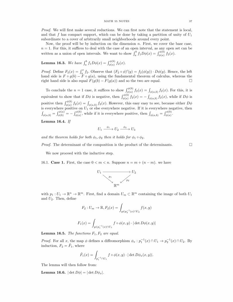
MATH 55 NOTES 37
Proof. We will first make several reductions. We can first note that the statement is local,and that f has compact support, which can be done by taking a partition of unity of U1
subordinate to a cover of arbitrarily small neighborhoods around every point.Now, the proof will be by induction on the dimension n. First, we cover the base case,
n = 1. For this, it suffices to deal with the case of an open interval, as any open set can be
written as a union of open intervals. We want to show∫ baf1Dφ(x) =
∫ φ(b)
φ(a)f2(x).
Lemma 16.3. We have∫ baf1Dφ(x) =
∫ φ(b)
φ(a)f2(x).
Proof. Define F2(x) =∫ xaf2. Observe that (F2 φ)′(y) = f2(φ(y)) ·Dφ(y). Hence, the left
hand side is F g(b) − F g(a), using the fundamental theorem of calculus, whereas theright hand side is also equal F (g(b)− F (g(a)) and so the two are equal.
To conclude the n = 1 case, it suffices to show∫ φ(b)
φ(a)f2(x) =
∫φ(a,b)
f2(x). For this, it is
equivalent to show that if Dφ is negative, then∫ φ(b)
φ(a)f2(x) = −
∫φ(a,b)
f2(x), while if Dφ is
positive then∫ φ(b)
φ(a)f2(x) =
∫φ(a,b)
f2(x). However, this easy easy to see, because either Dφ
is everywhere positive on U1 or else everywhere negative. If it is everywhere negative, then∫φ(a,b)
=∫ φ(a)
φ(b)= −
∫ φ(b)
φ(a), while if it is everywhere positive, then
∫φ(a,b)
=∫ φ(b)
φ(a).
Lemma 16.4. If
U1 U2 U3φ1 φ2
and the theorem holds for both φ1, φ2 then it holds for φ1 φ2.
Proof. The determinant of the composition is the product of the determinants.
We now proceed with the inductive step.
16.1. Case 1. First, the case 0 < m < n. Suppose n = m+ (n−m). we have
U1 U2
Rm
p1p2
with p1 : U1 → Rn → Rm. First, find a domain Um ⊂ Rm containing the image of both U1
and U2. Then, define
F2 : Um → R, F2(x) =
∫y∈p−1
2 (x)∩U2
f(x, y)
F1(x) =
∫y∈p−1
1 (x)∩U1
f φ(x, y) · | detDφ(x, y)|
Lemma 16.5. The functions F1, F2 are equal.
Proof. For all x, the map φ defines a diffeomorphism φx : p−11 (x) ∩ U1 → p−1
2 (x) ∩ U2. By
induction, F2 = F1, where
F1(x) =
∫p−11 ∩U1
f φ(x, y) · | detDφx(x, y)|.
The lemma will then follow from:
Lemma 16.6. |detDφ| = |detDφx|.
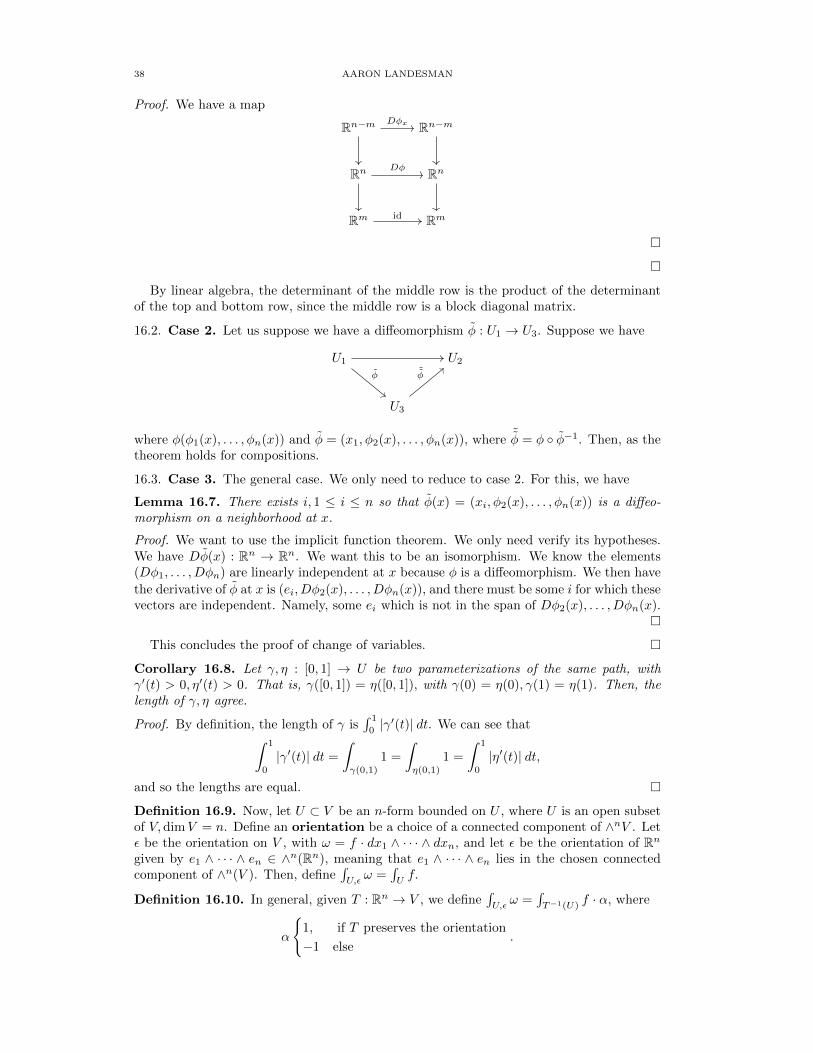
38 AARON LANDESMAN
Proof. We have a map
Rn−m Rn−m
Rn Rn
Rm Rm
Dφx
Dφ
id
By linear algebra, the determinant of the middle row is the product of the determinantof the top and bottom row, since the middle row is a block diagonal matrix.
16.2. Case 2. Let us suppose we have a diffeomorphism φ : U1 → U3. Suppose we have
U1 U2
U3
φ˜φ
where φ(φ1(x), . . . , φn(x)) and φ = (x1, φ2(x), . . . , φn(x)), where˜φ = φ φ−1. Then, as the
theorem holds for compositions.
16.3. Case 3. The general case. We only need to reduce to case 2. For this, we have
Lemma 16.7. There exists i, 1 ≤ i ≤ n so that φ(x) = (xi, φ2(x), . . . , φn(x)) is a diffeo-morphism on a neighborhood at x.
Proof. We want to use the implicit function theorem. We only need verify its hypotheses.We have Dφ(x) : Rn → Rn. We want this to be an isomorphism. We know the elements(Dφ1, . . . , Dφn) are linearly independent at x because φ is a diffeomorphism. We then have
the derivative of φ at x is (ei, Dφ2(x), . . . , Dφn(x)), and there must be some i for which thesevectors are independent. Namely, some ei which is not in the span of Dφ2(x), . . . , Dφn(x).
This concludes the proof of change of variables.
Corollary 16.8. Let γ, η : [0, 1] → U be two parameterizations of the same path, withγ′(t) > 0, η′(t) > 0. That is, γ([0, 1]) = η([0, 1]), with γ(0) = η(0), γ(1) = η(1). Then, thelength of γ, η agree.
Proof. By definition, the length of γ is∫ 1
0|γ′(t)| dt. We can see that∫ 1
0
|γ′(t)| dt =
∫γ(0,1)
1 =
∫η(0,1)
1 =
∫ 1
0
|η′(t)| dt,
and so the lengths are equal.
Definition 16.9. Now, let U ⊂ V be an n-form bounded on U , where U is an open subsetof V,dimV = n. Define an orientation be a choice of a connected component of ∧nV . Letε be the orientation on V , with ω = f · dx1 ∧ · · · ∧ dxn, and let ε be the orientation of Rngiven by e1 ∧ · · · ∧ en ∈ ∧n(Rn), meaning that e1 ∧ · · · ∧ en lies in the chosen connectedcomponent of ∧n(V ). Then, define
∫U,ε
ω =∫Uf.
Definition 16.10. In general, given T : Rn → V , we define∫U,ε
ω =∫T−1(U)
f · α, where
α
1, if T preserves the orientation
−1 else.
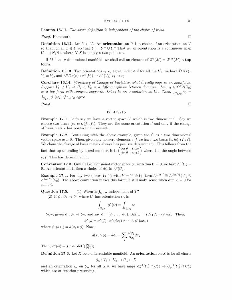
MATH 55 NOTES 39
Lemma 16.11. The above definition is independent of the choice of basis.
Proof. Homework
Definition 16.12. Let U ⊂ V . An orientation on U is a choice of an orientation on Vso that for all x ∈ U so that U = U+ ∪ U−.That is, an orientation is a continuous mapU → N,S. where N,S is simply a two point set.
If M is an n dimensional manifold, we shall call an element of Ωn(M) = Ωtop(M) a topform.
Definition 16.13. Two orientations ε1, ε2 agree under φ if for all x ∈ U1, we have Dφ(x) :V1 ' V2, and ∧nDφ(x) : ∧n(V1)→ ∧n(V2), ε1 7→ ε2.
Corollary 16.14. (Corollary of Change of Variables, what it really buys us on manifolds)Suppose V1 ⊃ U1 → U2 ⊂ V2 is a diffeomorphism between domains. Let ω2 ∈ Ωtop(U2)be a top form with compact supports. Let εi be an orientation on Ui. Then,
∫U2,ε2
∧2 =∫U1,ε1
φ∗(ω2) if ε1, ε2 agree.
Proof.
17. 4/9/15
Example 17.1. Let’s say we have a vector space V which is two dimensional. Say wechoose two bases (e1, e2), (f1, f2). They are the same orientation if and only if the changeof basis matrix has positive determinant.
Example 17.2. Continuing with the above example, given the C as a two dimensionalvector space over R. Then, given any nonzero elements e, f we have two bases (e, ie), (f, if).We claim the change of basis matrix always has positive determinant. This follows from the
fact that up to scaling by a real number, it is
(cos θ sin θsin θ cos θ
)where θ is the angle between
e, f . This has determinant 1.
Convention 17.3. Given a 0-dimensional vector space U , with dimV = 0, we have ∧0(U) =R. An orientation is then a choice of ±1 in ∧0(U).
Example 17.4. For any two spaces V1, V2 with V = V1 ⊕ V2, then ∧dimV ∼= ∧dimV1(V1)⊗∧dimV2(V2). The above convention makes this formula still make sense when dimVi = 0 forsome i.
Question 17.5. (1) When is∫U,ε
ω independent of T?
(2) If φ : U1 → U2 where Ui has orientation εi, is∫U1,ε1
φ∗(ω) =
∫U2,ε2
ω
Now, given φ : U1 → U2, and say φ = (φ1, . . . , φn). Say ω = fdx1 ∧ · · · ∧ dxn. Then,
φ∗(ω = φ∗(f) · φ∗(dx1) ∧ · · · ∧ φ∗(dxn)
where φ∗(dxi) = d(xi φ). Now,
d(xi φ) = dφi =∑j
∂φj∂xi
dxi
Then, φ∗(ω) = f φ · det(( ∂φi∂φj))
Definition 17.6. Let X be a differentiable manifold. An orientation on X is for all charts
φα : Vα ⊂ Uα → U ′α ⊂ Xand an orientation εα on Uα for all α, β, we have maps φ−1
α (U ′α ∩ U ′β) → U−1β (U ′β ∩ U ′α)
which are orientation preserving.
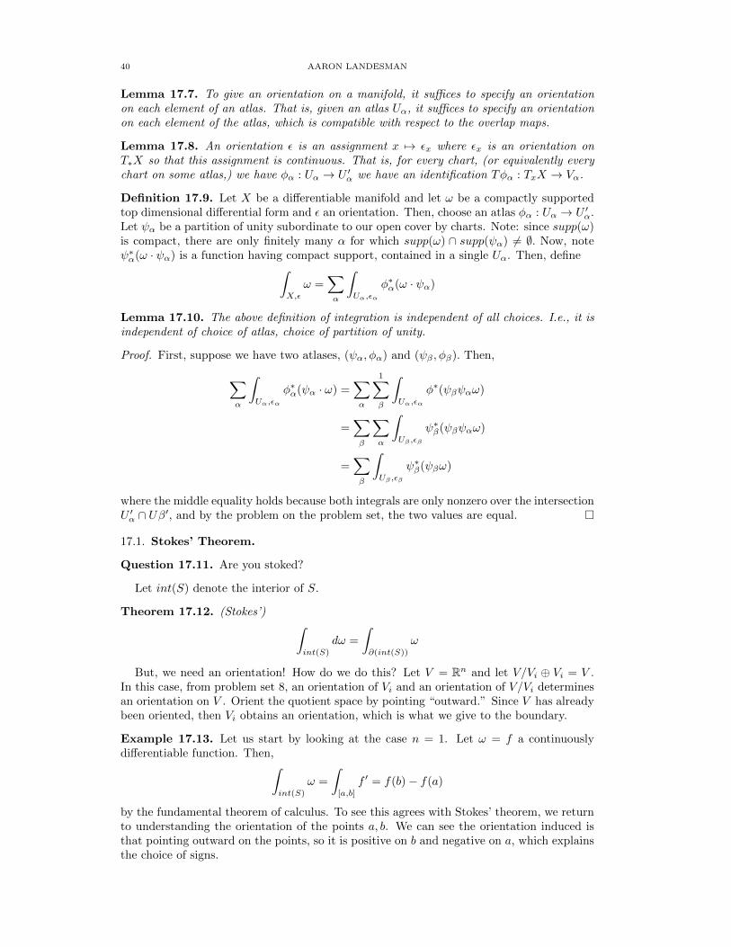
40 AARON LANDESMAN
Lemma 17.7. To give an orientation on a manifold, it suffices to specify an orientationon each element of an atlas. That is, given an atlas Uα, it suffices to specify an orientationon each element of the atlas, which is compatible with respect to the overlap maps.
Lemma 17.8. An orientation ε is an assignment x 7→ εx where εx is an orientation onT∗X so that this assignment is continuous. That is, for every chart, (or equivalently everychart on some atlas,) we have φα : Uα → U ′α we have an identification Tφα : TxX → Vα.
Definition 17.9. Let X be a differentiable manifold and let ω be a compactly supportedtop dimensional differential form and ε an orientation. Then, choose an atlas φα : Uα → U ′α.Let ψα be a partition of unity subordinate to our open cover by charts. Note: since supp(ω)is compact, there are only finitely many α for which supp(ω) ∩ supp(ψα) 6= ∅. Now, noteψ∗α(ω · ψα) is a function having compact support, contained in a single Uα. Then, define∫
X,ε
ω =∑α
∫Uα,εα
φ∗α(ω · ψα)
Lemma 17.10. The above definition of integration is independent of all choices. I.e., it isindependent of choice of atlas, choice of partition of unity.
Proof. First, suppose we have two atlases, (ψα, φα) and (ψβ , φβ). Then,
∑α
∫Uα,εα
φ∗α(ψα · ω) =∑α
1∑β
∫Uα,εα
φ∗(ψβψαω)
=∑β
∑α
∫Uβ ,εβ
ψ∗β(ψβψαω)
=∑β
∫Uβ ,εβ
ψ∗β(ψβω)
where the middle equality holds because both integrals are only nonzero over the intersectionU ′α ∩ Uβ′, and by the problem on the problem set, the two values are equal.
17.1. Stokes’ Theorem.
Question 17.11. Are you stoked?
Let int(S) denote the interior of S.
Theorem 17.12. (Stokes’) ∫int(S)
dω =
∫∂(int(S))
ω
But, we need an orientation! How do we do this? Let V = Rn and let V/Vi ⊕ Vi = V .In this case, from problem set 8, an orientation of Vi and an orientation of V/Vi determinesan orientation on V . Orient the quotient space by pointing “outward.” Since V has alreadybeen oriented, then Vi obtains an orientation, which is what we give to the boundary.
Example 17.13. Let us start by looking at the case n = 1. Let ω = f a continuouslydifferentiable function. Then,∫
int(S)
ω =
∫[a,b]
f ′ = f(b)− f(a)
by the fundamental theorem of calculus. To see this agrees with Stokes’ theorem, we returnto understanding the orientation of the points a, b. We can see the orientation induced isthat pointing outward on the points, so it is positive on b and negative on a, which explainsthe choice of signs.
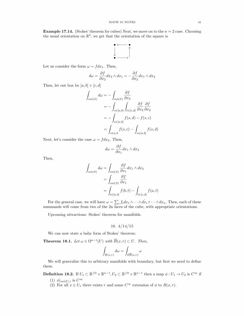
MATH 55 NOTES 41
Example 17.14. (Stokes’ theorem for cubes) Next, we move on to the n = 2 case. Choosingthe usual orientation on R2, we get that the orientation of the square is
• •
•
Let us consider the form ω = fdx1. Then,
dω =∂f
∂x2dx2 ∧ dx1 = − ∂f
∂x2dx1 ∧ dx2
Then, let out box be [a, b]× [c, d]∫int(S)
dω = −∫int(S)
∂f
∂x2
= −∫s∈[a,b]
∫t∈[c,d]
∂f
∂x2
∂f
∂x2
= −∫s∈[a,b]
f(s, d)− f(s, c)
=
∫s∈a,b
f(s, c)−∫s∈[a,b]
f(s, d)
Next, let’s consider the case ω = fdx2. Then,
dω =∂f
∂x1dx1 ∧ dx2
Then, ∫int(S)
dω =
∫int(S)
∂f
∂x1dx1 ∧ dx2
=
∫int(S)
∂f
∂x1
=
∫t∈[a,b]
f(b, t)−∫t∈[c,d]
f(a, t)
For the general case, we will have ω =∑i fidx1∧· · ·∧ ˆdxi∧· · ·∧dxn. Then, each of these
summands will come from two of the 2n faces of the cube, with appropriate orientations.
Upcoming attractions: Stokes’ theorem for manifolds.
18. 4/14/15
We can now state a baby form of Stokes’ theorem:
Theorem 18.1. Let ω ∈ Ωn−1(U) with B(x, r) ⊂ U . Then,∫B(x,r)
dω =
∫∂B(x,r)
ω
We will generalize this to arbitrary manifolds with boundary, but first we need to definethem.
Definition 18.2. If U1 ⊂ R≥0 ×Rn−1, U2 ⊂ R≥0 ×Rn−1 then a map φ : U1 → U2 is C∞ if
(1) φ|int(U1) is C∞
(2) For all x ∈ U1 there exists r and some C∞ extension of φ to B(x, r).
42 AARON LANDESMAN
Definition 18.3. Let X ⊃ ∂X be Hausdorff, second countable, paracompact topologicalspace. A structure of (X, ∂X) of a manifold with boundary is a collection of chartsR≥0 × Rn−1 ⊃ Uα → U ′α ⊂ X and φα(∂X) = Uα ∩ (0 × R−1), so that the transitionmaps are C∞ in the sense of Definition 18.2, and transition maps send the boundary to theboundary.
Example 18.4. We have M = B(x, 1) is a manifold with boundary. We can cover it withfour charts, corresponding to the 4 sets x > 0∩M, y > 0∩M, x < 0∩M, y < 0∩M .and the chart |(x, y)| < 1/2, where the first 4 charts are given by radially pushing out pointsto the strip (0, 1]× R.
Definition 18.5. Let (X, ∂X) be a manifold with boundary X → R. Then f is C∞ if forany chart containing x (equivalently for some chart containing x)
(1) f |int(X) is C∞
(2) ∀x, ∃r so that f extends to a C∞ function on B(x, r).
Definition 18.6. A k-differential form on (X, ∂X) is a form ω so that
(1) ω restricts to a k form on int(X) and(2) on any chart containing x, there exists an extension of ω to B(x, r).
Lemma 18.7. There is a natural restriction map Ωk(X)→ Ωk(∂X).
Proof. Fix x ∈ ∂X and fix a chart φα containing x. Extend φ∗(ω) to B(x, r) and restrict toB(x, r)∩Rn−1. Note that our choice of extension does not the restriction to the boundary,because the restriction of ω to the boundary is determined by continuity on the part of theball corresponding to R>0 × Rn−1.
Definition 18.8. An orientation on (X, ∂X) is an orientation on the interior.
Definition 18.9. Given (X, ∂X), ω ∈ Ωk(X) and an orientation ε, we can define∫X,ε
ω.
Using a partition of unity, we can assume that Supp(ω) ⊂ Uα and is compactly supported.Then, define ∫
U ′α,ε
ω =
∫int(Uα),ε
φ∗α(ω).
Lemma 18.10. Let ε be an orientation on the interior of (X, ∂X). This induces an orien-tation on ∂X.
Proof. First, let us deal with the case of a chart (U, φ). Let x ∈ ∂U . We want to orientRn−1. We write the exact sequence
0 Rn−1 Rn Rn/Rn−1 0
and an isomorphism ∧n(Rn) ∼= Rn/Rn−1 ⊗ ∧n−1(Rn−1). From this, it suffices to orientRn) and Rn/Rn−1. The orientation for Rn comes from the orientation on X, as the n ballaround x is oriented. We need to orient Rn/Rn−1, and we orient this so that the “outward”direction is positive. More explicitly, let γ : (−ε, ε)→ U be a path so that Dγ ∈ Rn projectsto a positive vector on Rn/Rn−1.Then, for all sufficiently small t we have γ(t) /∈ U .
Theorem 18.11. Let (X, ∂X) be a manifold with boundary, and ω ∈ Ωn−1(X) with compactsupport. Then, ∫
X,ε
dω =
∫∂X,ε
ω
Proof. Since ω has compact support, we can write ω =∑α ωψα is a finite sum, and if we
show this for ω, η it automatically holds for ω + η. So, we may reduce to the case thatsupp(ω) ⊂ Uα. It remains to show∫
Uα,ε
d(φ∗ω) =
∫∂Uα,ε
φ∗ω
MATH 55 NOTES 43
Now, take a box containing Uα, and extend by 0. We are now done, because we have alreadyshown stokes’ theorem on boxes.
Corollary 18.12. If X is a n-manifold with no boundary and ω ∈ Ωn−1(X) then∫X,ε
dω =0.
Proof. Use stokes’ theorem and the fact that∫X,ε
ω = 0.
19. 4/16/15
We will now begin complex analysis!
Definition 19.1. A function f : U → C is complex differentiable at x ∈ U if thereexists λ ∈ C so that
lim|v|→0
f(x+ v)− f(x)− λ · v|v|
= 0
Remark 19.2. Recall that f is differentiable as a function U → R2 at x ∈ U if there existsT ∈ HomR(C,C) so that
lim|v|→0
f(x+ v)− f(x)− T (v)
|v|= 0
The difference is that in one case we require T to be multiplication by a complex number.That is T ∈ HomR(C,C) instead of T ∈ C ∼= HomC(C,C). So, T comes from a complexnumber λ if T multi = multi T . That is T commutes with
multi =
(0 −11 0
)Corollary 19.3. (Cauchy-Riemann) Let f : U → C be differentiable in the real sense.Then, f = fR + i · fI is complex differentiable if and only if(
∂fR∂x
∂fR∂y
∂fI∂x
∂fI∂y
)·(
0 −11 0
)=
(0 −11 0
)·
(∂fR∂x
∂fR∂y
∂fI∂x
∂fI∂y
)Expanding this out gives
∂fR∂y
= −∂fI∂x
∂fR∂x
=∂fI∂y
Proof. Follows from the prior discussion of complex differentiable functions.
Remark 19.4. We will see
polynomials ⊂ complex differentiable ⊂ C∞-functions
Complex differentiable functions are also called holomorphic or analytic
Example 19.5. (1) If f1, f2 are holomorphic then so are f1 + f2, f1 · f2.(2) The functions f(z) = 0, f(z) = 6, f(z) = z are holomorphic. In general, any
polynomial, f(z) =∑ki=0 ciz
i with ci ∈ C are complex differentiable.(3) If U = C \ 0 then f(z) = 1
z is differentiable.
(4) f(z) = exp(z) =∑∞n=0
zn
n! , which converges by one of our convergence tests.
Notation 19.6. When we write f ′(z) we mean the value of λ from definition 19.1.
Lemma 19.7. We have exp′(z) = exp(z)
Proof. We have exp(z + v) = exp(z) · exp(v) and viewed as a function of z, plugging inz = 1, we obtain the result.
44 AARON LANDESMAN
Lemma 19.8. If
U1 U2 U3f g
with f, g holomorphic, then g f is holomorphic with (g f)′(x) = g′(f(x)) · f ′(x)
Proof. The composition of the two maps has differential which is the product of the twoderivatives coming from Definition 19.1.
Lemma 19.9. If f : U1 → U2, g : U2 → U1 are complex differentiable homeomorphismswith f ′(x) 6= 0 then f−1(x) is also complex differentiable. Further, f−1(y)′ = 1
f ′(f−1(y))
Proof. We know by the inverse function theorem, we have that f−1 is differentiable. By theinverse function theorem, if a map is given by multiplication by a complex number, then theinverse map is given by multiplication by the inverse complex number, hence the inverse isholomorphic.
Let U ⊂ Rn and consider ΩnC(U) = Ωn(U)⊗R C. Let ω ∈ Ωn(U) with ω = ωR + iωI .
Lemma 19.10. Note that
(1) Ω•C(U) is a ring
(2) d : Ω•C(U)→ Ω•+1C (U)
(3) Given φ : U1 → U2, we have a map φ∗ : Ω•C(U2)→ Ω•C(U1)(4) d φ∗ = φ∗ d(5) We have df = Df .
Proof. Omitted, analogous to the real case.
Let f be a holomorphic function which is C1 on a domain U . Let z0 ∈ U and B(z0, r) ∈ U .
Then, f(z)z−z0 is a complex valued function on U \z0. Note that z ∈ Ω0
C(U). Then, dz ∈ Ω1C(U).
We can write z = x+iy. Then, dz = dx+idy. Now, consider the function f(z)z−z0 dz ∈ Ω1
C(U\z).
Remark 19.11. The assumption that it is C1 is not needed, which will be shown later,possibly on homework.
Lemma 19.12. (Cauchy Integral Formula)∫S(z0,r)
f(z)
z − z0dz = 2πi · f(z0)
independent of r.
Remark 19.13. Using the fact that we can exchange integration and differentiation, it isvery easy to differentiate f with respect to z0, and show it is infinitely differentiable.
Proof.
Lemma 19.14. Let f be C1. Then, f is holomorphic if and only if d(fdz) = 0.
Proof. Letting f = fR + ifI we have
d((fR + ifI) · (dx+ i dy)) =∂fR∂x
dx ∧ dx+∂fR∂y
dy ∧ dx− ∂fI∂x
dx ∧ dy − ∂fI∂y
dx ∧ dy
+ i · (∂fI∂x
dx ∧ dx+∂fI∂y
dy ∧ dx+∂fR∂x
dx ∧ dy +∂fR∂y
dy ∧ dy)
= −(∂fR∂y
+∂fI∂x
dx ∧ dy) + i(∂fR∂x− ∂fI
∂xdx ∧ dy)
Then, these are precisely the Cauchy Riemann equations, so it is 0 if and only if the functionis holomorphic.
MATH 55 NOTES 45
Corollary 19.15. If we have two circles containing z0 the value of∫S(a,r1)−S(b,r2)
f(z)
z − z0dz
is independent of the choice of circles so long as the annulus between the circles is containedin U .
Proof. Apply stokes theorem to the annulus. We orient the annulus by the inherited orien-
tation from R2. Let ω = f(z)z−z0 dz. Then,∫
X,ε
dω =
∫∂X
ω
Note the left hand side is 0 by the previous lemma, since f(z)z−z0 is holomorphic. The right
hand side is imply the integral over the outer circle minus the integral over the inner circle.So, the integral is independent of the choice of circle.
Let us now prove the theorem in steps.
19.1. Case 1: f(z) = 1, z0 = 0, and S is the circle of radius 1 centered at 0. Wewish to calculate
intSdz
z= 2πi
We can do this by parameterizing the circle, R → S, t 7→ exp(it) = φ(t). Let us calculateφ∗(dzz ) ∈ Ω1
C(R).
Lemma 19.16. φ∗(dzz ) = i dt.
Proof. We see this is φ∗(dz)zφ = d(zφ)
zφ and z φ : R → C, t 7→ exp(it). Then, the ratiod(exp(it))
zφ = i dt.
Now, using change of variables,∫S,ε
dz
z=
∫[0,2π]
φ∗(dz
z)
Note that the function φ : [0, 2π] → S is not an isomorphism, but it is on the open set(0, 2π) and the function is bounded, and the integral on the open integral is equal to theintegral on the closed interval.
19.2. Case 2: General f , with z0 = 0. We claim∫Sr
f(z)− f(0)dz
z= 0
which certainly implies the theorem, as we can reduce to the case of a constant function. Tosee this, we can make r arbitrarily small, as the left hand side is independent of the valueof r. We can see
∫Sr
f(z)− f(0)dz
z=
∫[0,2π]
φ∗(dz
z)(f(z)− f(0)) φ
= i
∫[0,2π]
f(r exp(it))− f(0)
Now, since the function is continuous, this value is arbitrarily small, hence, it must be 0.
19.3. Case 3: General Case. Compose with translation by z, so we can assume z = 0and reduce to case 2.
46 AARON LANDESMAN
20. 4/21/15
Question 20.1. Is∫f =
∫f dz?
Their values agree, but in some sense they are different objects, as in one case we areintegrating a function, and in another we are integrating a 1-form. If we wanted to, wecould define
∫f(x) =
∫f(x) dx.
Theorem 20.2. (Maximum Principle) Suppose we have a domain U and a disk B(z0, r) ⊂U. Then, |f(z0)| ≤ maxz∈∂B(z0,r) |f(z)|. In fact,
∫∂B(z0,r)
f(z) = f(z0).
Proof. Let S = ∂B(z0, r). Using Cauchy-Riemann, we have
f(z0) =1
2πi
∫S
f(z)dz
z − z0
Let us assume now z0 = 0, as can be done by composing with translation. Then, we have amap [0, 2π]→ S, t 7→ exp it. ∫
S
f(z) dz
z= i
∫t∈[0,2π]
f(exp it)
Therefore,
|∫S
f(z) dz
z| = |i
∫t∈[0,2π]
f(exp it)|
≤∫
[0,2π]
|f(exp(it))|
≤∫
0,2π
maxz∈S|f(z)|
= 2πmaxz∈S|f(z)|
Definition 20.3. An entire function is an analytic function C → C. I.e., defined on theentire complex plane.
Theorem 20.4. (Louiville’s Theorem) Let f be holomorphic on all of C and for all ε thereis some R so that |f(z)| < ε for |z| > R then f = 0.
Proof. Pick z0. We want to show f(z0) = 0. For all ε, draw a circle around z0 of radius R,and apply the maximum principle, Theorem 20.2.
Corollary 20.5. (Fundamental Theorem of Algebra) Any complex polynomial has a root.
Proof. Suppose there is no z so that p(z) = 0. Suppose there is such a polynomial f . Notethat f → ∞ as z → ∞. Consider 1
f . Note it is holomorphic. Note that | 1f | < ε for R
sufficiently large, as the highest term dominates, i.e., the if f(z) = azn + · · · we have f(z)is approximately azn, which goes to ∞ for |z| → ∞. So 1
f = 0, a contradiction.
Remark 20.6. Thanks to Wyatt Mackey for taking the rest of today’s notes, as I was away,at a talk of J.P. Serre.
Theorem 20.7. Let f be holomorphic and C1 on U . Then f is C∞.
Proof. It suffices to show f ′ is C1 by problem 8 on the PSet. Take any ball B ⊆ U
with z0 ∈ B, then f(z0) =∫Sf(z)dzz−z0 . Partials exist by the midterm, as we have ∂fR
∂x0=
12πi
∫∂∂x0
( 1z−z0 )f(z)dz, and the inner term is clearly differentiable with respect to z0. Then
it continues to satisfy the Caucy-Riemann equations after you do the integration, whichfinishes the problem.
“We’ll now state the following false theorem.” –Gaitsgory
MATH 55 NOTES 47
Theorem 20.8. Let f be C∞ on (a, b) such that for some x ∈ (a, b), f (n) = 0. Then f = 0.
We’ve already seen this is false–consider for instance e−1x at x = 0.
“This is completely false in the real world.” – Gaitsgory
However,
Theorem 20.9. Let f be holomorphic on U and B ⊆ U a disk of radius r, with z0 the
center. Then f(z) =∑ f(n)(z0)
n! (z − z0)n uniformly and absolutely on B.
Proof. By the Cauchy Integral Formula, f(z) = 12πi
∫S
f(z)(z−z) , where S is a circle slightly
larger than B.
“No, z′ isn’t good, what should we use... Ah, z.” –Gaitsgory (paraphrased)
Then 1z−z = 1
z (1 + zz + z2
z2 + ...) converges uniformly and absolutely, by taking the radius of
S to be r0, so that | zz | <rr0< 1. Then gn → g uniformly implies
∫Sgn →
∫Sg, so we are
left with∫ f(z)dz
z (∑∞n=m
zn
zn ), which we want to bound < ε, which is clear. This will show
that the sequence∑ni=0(
∫Sf(z)zi+1 )zi converges to f(z).
Now f(n)(0)n! = 1
2πi
∫f(z)dz · ( 1
z−z0 )(n)|z0=0, which follows by the Cauchy formula on
f (n)(0).
Theorem 20.10. Let ai be a sequence of complex numbers such that lim sup n√|an| ≤ 1
r0.
Then the series∑anz
n converges pointwise to a holomorphic function on Br, and theconvergence is uniform on Br, for any r < r0.
Proof. First, uniform convergence on Br: Take r < r′ < r0, then for all but finitely manyn, n√|an| < 1
r′ =⇒ |an| < 1(r′)n , so |anzn| < ( rr′ )
n, which we know how to estimate. Then
the tails are ≤∑∞n=m( rr′ )
n = ( rr′ )m( 1
1− rr′
).
We now need a lemma. In particular, if fn → f uniformly on some domain in U , withfi holomorphic, then we’d like to claim f is as well. This will be presented below. Thenwe can apply this to our case to get that our function is holomorphic, and then by writingBr0 = ∪r<r0Br, we get our theorem. (Note that our functions are holomorphic on Br, so afortiori they are holomorphic on Br.)
We used the following lemma in our theorem:
Lemma 20.11. Let fn → f uniformly on U be holomorphic. Then f is holomorphic.
Proof. We have f(z0) = lim fn(z0) = lim 12πi
∫S
dzz−z0 fn(z) = 1
2πi
∫dzz−z0 f(z), hence the limit
is a holomorphic function.
Theorem 20.12. Let U0 ⊆ U and f0 a holomorphic function on U0. Assume U is con-nected. Then there is at most one f on U such that f |U0 = f0. (We say that there is atmost one analytic continuation of f0.)
Proof. Let f1, f2 be two holomorphic extensions, then (f1 − f2)|U0= 0. We may therefore
assume that f0 = 0, and we wish to show f = 0. Set V n = z ∈ U | f (n)(z) = 0. Notethese are closed sets. Then write V = ∩nV n, and the intersection of closed sets is closed,so V is closed as well.
We claim that V is also open in U . Given z ∈ V , there is a disk B ⊆ U around z. On B,
f(z) =∑ f(n)(z0)
n! (z − z0)n = f = 0 on all of B, so V contains B =⇒ V is open. Then Uconnected implies V = U .
On Thursday we will study the geometry of holomorphic mappings. Suppose U1, U2 are
domains, and U1f−→ U2. Then f is biholomorphic if f, f−1 are both holomorphic.
Example 20.13. Take U1 = C and U2 = B. There are diffeomorphisms between C and Bthrough stereographic projections. However, we’ll prove that there is not a biholomorphicmap between the two.
48 AARON LANDESMAN
Theorem 20.14. (Liouville) A bounded holomorphic function on C is constant.
From this, we can conclude C 6= B.
Example 20.15. Take U1 = C and U2 = z ∈ C | Im(z) > 0. Here U2 is holomorphic toB by the map exp(iz), so U2 = B 6= C holomorphically.
We will also show that all transforms of C are of the form az + b. Similarly, U2 fromExample 20.15 (the upper half plane) may be manipulated exclusively by maps of the formz 7→ az+b
bz+a.
21. 4/23/15
Theorem 21.1. Let U0 → C with U0 ⊂ U connected. Then f0 admits at most one extensionto a holomorphic function on U .
Proof. This follows from the identity principal. That if two holomorphic functions agree onan open set, they agree everywhere.
Lemma 21.2. Consider f(z) = 1z . Take B(1, r) with r < 1. Then there exists log z :
B(1, r)→ C so that log′(z) = 1z . Then, log z can be analytically extended to the complement
of any ray ending at the origin.
Proof. Consider the map exp : C→ C \ 0 given by
sz|θ < Re(z) < θ + 2π → w ∈ C \ ray
Lemma 21.3. f f : U1 → U2 is holomorphic and f ′ 6= 0, bijective, then f−1 is a holomorphicfunction. I
Proof. This follows from the following lemma, as we showed previously in class, as theinverse of a complex number is a complex number.
Lemma 21.4. If f : U1 → U2 is a C∞ function with Df(x) an isomorphism for all x ∈ U1
and f is bijective, then f−1 is C∞.
Proof. We know that for every x there is a small ball around x so that on this ball, thisfunction has an inverse. Since f is C∞ its inverse is also C∞ by repeated applications ofthe inverse function theorem.
Using the above lemma, we have that log is the inverse of this map.
Remark 21.5. In fact, as we approach the ray from different directions, the values willdiffer by 2πi. That is, we can locally analytically extend log but not globally.
Example 21.6. We can define z1/n for n ∈ N given by exp( 1n log z). Alternatively, we can
define the map f : C\0→ C\0, w 7→ wn. We have a map from a slice of angle 2π/n to C\0given by z 7→ zn and the inverse function is z1/n. This cannot be defined on all of C, but ifwe go around a circle and take the limit from both sides, they will differ by exp(2πi/n). Wesay these functions are multi-valued functions though we won’t use this terminology.
21.1. Meromorphic Functions. Recall the following problem from the problem set:
Proposition 21.7. Let f : U → C with f(z0) = 0. Then, f(z)z−z0 extends to a holomorphic
function on U .
Proof. Without loss of generality, assume z0 = 0. Then, we can write f(z) =∑n≥0 anz
n.
Then, f(z)z =
∑n≥1 anz
n−1. This series also converges on some region around 0, whichholds as the coefficients of a holomorphic function are bounded by a geometric series, andthe derivative will have the same radius of convergence.
MATH 55 NOTES 49
Definition 21.8. A holomorphic function f : U \ z0 → C can be extended to a meromor-phic function f : U → C if there is some n so that f(z)(z− z0)n extends to a holomorphicfunction on U . In this case, the function is said to be meromorphic at z0.
Remark 21.9. Heuristically, meromorphic functions can be obtained by starting with aholomorphic function f and then divide by a power of z− z0. In particular, all holomorphicfunctions are meromorphic. Further, one can say that a function is meromorphic if and onlyif at all points, its Laurant expansion only has finitely many negative terms.
Lemma 21.10. Any meromorphic function f , we can write f(z) =∑n≥k anz
n for somepossibly negative k ∈ Z.
Proof. Apparent from the fact that holomorphic functions being equal to their taylor seriesaround any point, and the definition of a meromorphic function.
Definition 21.11. A holomorphic function f : U \ z1, . . . , zn → C is meromorphic if fis meromorphic on some small disc around zi, which is in turn equivalent to the existenceof some mi so that f(z) ·
∏i(z − zi)mi extends to a holomorphic function on U .
Definition 21.12. Let f : U\z1, . . . , zn → C be meromorphic. Let f =∑n≥k an(z−z0)k.
Then, define the residue at zi be Reszi(f) = a−1.
Theorem 21.13. Let f : U \z1, . . . , zn → C be a meromorphic function. Let B ⊂ U, andlet S be the boundary of B. Then,
∫Sf(z)dz = 2πi
∑zi∈B Reszif.
Proof. Use Stokes’ theorem. Consider the manifold where we remove small open circlesaround each of the poles in S. This is a manifold with boundary, and the integral over it is0 by stokes’ theorem, as the function is analytic on this manifold. Therefore,∫
S,ε
f(z) dz +∑i
∫Si,−ε
f(z) dz = 0
Note that the key step is that the small circles are oriented with the opposite orientationfrom the standard orientation.
To complete the proof, it suffices to compute the integral of a small disk around a point.Let T be one of the small circles around a point. That is, it suffices to show∫
T
dz
zn=
0 if n > 1
2πi if n = 1
The latter case was shown in class by Cauchy’s formula. It suffices to show the case n > 1,which was done on homework. This can be done by performing a change of variables totransfer it to a line segment, and then computing it explicitly.
Example 21.14. Suppose f(z) = P (z)Q(zx) where Q(z) has no real roots and degQ ≥ degP+2.
We will compute ∫(−∞,∞)
= limΛ→∞
∫[−Λ,Λ]
f(x)
Theorem 21.15. Let R(f) be the ramification locus of f , which is the set of points ziat which f has a pole at zi. Then,∫
(−∞,∞)
= 2πi∑
zi∈R(f)
Reszif
Proof. Integrate over a large semicircle. We then have∫[−Λ,Λ]
f(z) dz +
∫arch
f(z) dz = 2πi∑
zi∈R(f)
Reszif
This equality follows from the same sort of procedure as Theorem 21.13. It suffices to show∫arch
f(z) dz = 0. To see this, note that f(z)|arch ∼ 1Λ2 while len(arch) ∼ Λ. Then, the
integral is the ratio of these in the limit, ΛΛ2 = 1
Λ → 0 as Λ→∞.
50 AARON LANDESMAN
Definition 21.16. Define the Upper half plane, H = z|im (z) > 0 and the unit diskB = z||z| < 1.
Definition 21.17. We have an action of GL2(R)+, the group of real 2×2 invertible matrices
with positive determinant, acting on H by
(a bc d
)7→ (z 7→ az+b
cz+d . Note that all diagonal
matrices act trivially, so we have that GL2(R)+/R≥0. The group of Linear fractionaltransformations is GL2(R)+/R≥0.
Lemma 21.18. We have a biholomorphism H ∼= B.
Proof. Take f : H→ B, z 7→ z−iz+i with inverse w 7→ i(w+1)
1−w .
Theorem 21.19. Every automorphism of H is given by a linear fractional transformation.
Proof. Using the biholomorphism above, we can translate automorphisms on H to auto-morphisms on B by conjugating by the biholomorphism given. If we start with the linearfractional transformation w 7→ aw+b
cw+b with a = −d, b = −c. Then, this is sent to the auto-
morphism z 7→ eiθ(a−z)1−az . Note such automorphisms send 0 7→ a. So to complete the proof,
by composing with a translation, it suffices to show the only automorphisms fixing 0 arerotations. That is
Theorem 21.20. Any automorphisms of B with f(0) = 0 is given by multiplication by eiθ.
Proof. To prove this, we will employ the following lemma
Lemma 21.21. (Schwarz Lemma) If f : B → B is holomorphic with f(0) = 0 and |f(z)| ≤|z| then, if the equality takes place for at least one z0 ∈ B then f(z) = eiθz.
Recall the maximum principle. That if f is holomorphic in some ball B ⊂ U thenmaxz∈B |f(z)| is acheived on the boundary.
Proof. By assumption f(0) = 0. By the homework, we obtain a well defined function
φ(z) = f(z)z . It suffices to show |φ(z)| ≤ 1 and if equality is achieved at some z0 6= 0, z0 ∈ B
then φ(z) is constant. We can now apply the maximum principle.
Assuming the above lemma, we have f(z) ≤ z and |f−1(w)| ≤ |w|. Taking w = f(z) wehave |f(z)| ≤ |z| ≤ |f(z)|, so we obtain a point at which |f(z)| = |z| and by the schwartzlemma, f is a rotation. It suffices to prove |φ(z)| ≤ 1
r for all r < 1. Consider the disk ofradius r inside the unit disk. Applying the maximum principle to φ on the disk of radius r.Note that |φ(z)| ≤ maxz∈Sr |φ(z)| ≤ 1
r . From the second part of the maximum principle, iff acheives its maximum on the interior, it is constant.
22. 4/28/15
Today, we will prove the Riemann Mapping Theorem.
Theorem 22.1. (Riemann Mapping Theorem) Let U ⊂ C be a simply connected domain.Then, there exists a biholomorphism U ∼= B(0, 1).
Proof. We’ll prove this theorem in four steps.
22.0.1. Step 1: Desired properties of the biholomorphism. Cosider the set S of injectivefunctions U → B(0, 1). Pick any z0 ∈ U . Consider the map S → R≥0, f 7→ |f ′(z0)|. Let Fbe the element of S so that |F ′(z0)| ≥ |f ′(z0)| for all f ∈ s.
Let us assume S is nonempty and the maximum derivative is attained by some function,and that F has holomorphic inverse. We will show this later. We now prove two desiredproperties of such a biholomorphism, assuming one exists.
Lemma 22.2. (1) Let F (z0) = 0.
MATH 55 NOTES 51
(2) F is surjective.
Proof. Suppose F (z0) 6= 0. Then,
G(z) =F (z)− F (z0)
1− F (z0)F (z)
G′(z0) =F ′(z0)
1− |F (z0)|2
Note that if F is injective, so is G, as the map w 7→ w−F (z0)
1−F (z0)wis an automorphism. But the
absolute value of |G′(z0)| > |F ′(z0)| contradicting the fact that F has maximum derivativeat 0.
Next, we will show F is surjective. Say w /∈ Im(F (z)). Consider
H0(z) =F (z)− w
1− w · F (z)
H1(z) =√H0(z)
H2(z) =H1(z)−H1(z0)
1−H1(z0)H1(z)
Note that H1 is defined because U is simply connected and H0 never vanishes. This is wherewe crucially use simply-connectedness of U . Either square root of H0 will do. Note that H1
is injective if H0 is. Observe
H ′2(z0) =1 + |w|2√|w|· F ′(z0)
Note that 1+|w|2√|w|
> 1.
22.0.2. Step 2: Such an F is a biholomorphism.
Lemma 22.3. Let f be an injective map U → C. Then f ′(z) 6= 0 for all z ∈ U .
Proof. We may assume f(0) = 0 and f ′(0) = 0. Write f(z) = zng(z) = (zh(z))n. Then,zh(z) is biholomorphic on a sufficiently small disk around the origin. Then, the derivativeof (zh(z))′ = h(0) 6= 0. So, f(z) is the composition (z 7→ zn) (z 7→ z · h(z)). Hence, anybiholomorphism must have nonzero derivative at every point.
Hence, F is in fact a biholomorphism.
22.0.3. Step 3: There exists some injective holomorphic function. We want to produce aninjective holomorphic function U → B(0, 1). Suppose a /∈ U . Then, there is some element
b /∈ U , because U is simply connected. Consider φ1 =√
z−az−b and let φ2 be the other
squareroot. We could even take√z − a, and proceed with the same proof.
Lemma 22.4. We have φ1(z′) = φ1(z′′) =⇒ z′ = z′′, φ2(z′) = φ2(z′′) =⇒ z′ = z′′.
Proof. Observe z′−az′−b = z′′−a
z′′−b =⇒ z′ = z′′.
Note φ1, φ2 have non-vanishing derivative, so they are open maps. Let w ∈ Im(φ1).There is some r so that B(w, r) ∈ Im(φ1) and B(w, r) ∩ Im(φ2) = ∅. Consider
f(z) =r
w − φ2(z)
Note that f(z) ∈ S, since φ2(z) is injective.
52 AARON LANDESMAN
22.0.4. Step 4: The maximum is attained. Recall
S = injective holomorphic maps U → B(0, 1)α : S → R, f 7→ |f(z0)|
Theorem 22.5. Let R be any set of holomorphic functions on U so that there exist Λ with|f(z)| ⊂ Λ for all f ∈ S, z ∈ U . Then, any sequence fn ∈ S has a subsequence that convergesuniformly for all compact K ⊂ U .
Proof. Write U = ∪nKn for Kn compact, Kn ⊂ Kn+1. Using this, it is enough to show thefollowing proposition, as we can then applying to each Kn in the above cover sequentially.
Proposition 22.6. Let R be any set of holomorphic functions on U so that there exist Λwith |f(z)| ⊂ Λ for all f ∈ S, z ∈ U . For every compact K ⊂ U , and sequence fn, thereexists a subsequence that converges uniformly on K.
The difference between this and the previous theorem, is that here we only have to do iton a given compact, whereas in the theorem, we have to do it for all compact sets.
Proof. Note that using compactness of K, there exists r so that for all x ∈ K,B(x, r) ⊂ U .
Lemma 22.7. The sequence fn|K is equicontinuous.
Proof. For every ε > 0 we must find δ so that for all z1, z2, n, |z1 − z2| ≤ δ =⇒ |fn(z1)−fn(z2)| ≤ ε. We will show for all ε, there is some δ so that
| 1
|z − z1− 1
z − z2| < ε
for all z ∈ ∂B(z1, r) for all |z1 − z2| < ε/rΛ. Now, let
f(z1) =1
2πi
∫∂B(z1,r)
f(z) dz
z − z1
f(z2) =1
2πi
∫∂B(z1,r)
f(z) dz
z − z2
Then, by assumption,
|f(z1)− f(z2)| < 1
2πi
∫f(z) dz(
1
z − z1− 1
z − z2) ≤ r2π
2πΛ · ε
Λr
using Cauchy’s integral formula. I.e., Cauchy’s integral formula shows uniform boundednessimplies equicontinuity on every compact.
By the Arzela-Ascoli theorem, from the midterm, we obtain a convergent subsequence.
Theorem 22.8. (Hurwitz) Let fn → f converge uniformly on every compact set. Then, iff is nonconstant and fn are injective, then so is f .
Proof.
Theorem 22.9. If fn → f on z0 ∈ U with f(z0) = 0, f 6= 0. If f(z0) = 0, for every r thereis some N so that for all n ≥ N , we have that Fn will have a zero on B(z0, r).
Proof. In a failed attempt to prove 22.9, we provide the following theorem.
Theorem 22.10. Let f and g be holomorphic on U so that |g| < |f |. If f has a zero onsome B(z0, r) then so does f + g.
Proof. Take f + g = f(1 + gf ). Note that g
f is a well defined holomorphic function, as
if f(z0) = 0, then f(z) = (z − z0)nh(z), and g(z) = (z − z0)mi(z) where m > n as fis everywhere bigger in absolute value. Hence, the ratio is a well defined holomorphicfunction.
MATH 55 NOTES 53
Here is a more successful attempt to prove 22.9.
Theorem 22.11. Let g be holomorphic on U , and B(z0, r) ⊂ U and g has no zeros on∂B(z0, r). If ∫
∂B(z0,r)
g′(z)
g(z)dz 6= 0
then g has zeroes in B(z0, r).
Proof. Immediate, for example, one can take the taylor expansion of f locally.
Remark 22.12. In fact, we have∫∂B(z0,r)
g′
gdz = 2πi
∑z∈∂B(z0,r)
ordz(f).
Let us see why 22.11 implies 22.9. Tak fn → f . Then, f ′n → f ′, so∫ f ′nfndz →
∫f ′
f dz.
Let us see why 22.9 implies 22.8. If f(z′) = f(z′′) then consider fn(z) − fn(z′′) →f(z)− f(z′′). Take r so that z′′ /∈ B(z′, r). Note g(z′) = 0, so for all n large enoguh, thereis some z′′′ ∈ B(z′, r) so that gn(z′′′) = 0. Hence, fn(z′′′) − fn(z′′) = 0. Because fn isinjective, we have z′′′ = z′′, contradicting that z′′ /∈ B(z′, r).
Let us see why the maxumim is attained, using the above two theorems. Consider fn → fso |f ′n(z0)| → supf∈S |f ′(z0)|. Then, f is injective by the second theorem. The supremumexists because it is equal to the derivative of f .