MATH 567: Mathematical Techniques in DataScienceLab 8

Dominique Guillot

Departments of Mathematical Sciences

University of Delaware

April 11, 2017

1/14

Recall

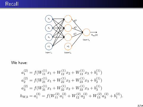
We have:

a(2)1 = f(W

(1)11 x1 +W

(1)12 x2 +W

(1)13 x3 + b

(1)1 )

a(2)2 = f(W

(1)21 x1 +W

(1)22 x2 +W

(1)23 x3 + b

(1)2 )

a(2)3 = f(W

(1)31 x1 +W

(1)32 x2 +W

(1)33 x3 + b

(1)3 )

hW,b = a(3)1 = f(W

(2)11 a

(2)1 +W

(2)12 a

(2)2 +W

(2)13 a

(2)3 + b

(2)1 ).

2/14

Recall (cont.)

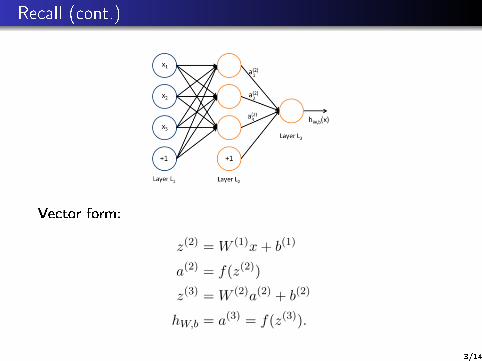
Vector form:

z(2) =W (1)x+ b(1)

a(2) = f(z(2))

z(3) =W (2)a(2) + b(2)

hW,b = a(3) = f(z(3)).

3/14

Training neural networks

Suppose we have

A neural network with sl neurons in layer l (l = 1, . . . , nl).

Observations (x(1), y(1)), . . . , (x(m), y(m)) ∈ Rs1 × Rsnl .

We would like to choose W (l) and b(l) in some optimal way for all

l.

Let

J(W, b;x, y) :=1

2‖hW,b(x)−y‖22 (Squared error for one sample).

De�ne

J(W, b) :=1

m

m∑i=1

J(W, b;x(i), y(i)) +λ

2

nl−1∑l=1

sl∑i=1

sl+1∑j=1

(W(l)ji )

2.

(average squared error with Ridge penalty).

Note:

The Ridge penalty prevents over�tting.

We do not penalize the bias terms b(l)i .

4/14

Training neural networks

Suppose we have

A neural network with sl neurons in layer l (l = 1, . . . , nl).

Observations (x(1), y(1)), . . . , (x(m), y(m)) ∈ Rs1 × Rsnl .

We would like to choose W (l) and b(l) in some optimal way for all

l.

Let

J(W, b;x, y) :=1

2‖hW,b(x)−y‖22 (Squared error for one sample).

De�ne

J(W, b) :=1

m

m∑i=1

J(W, b;x(i), y(i)) +λ

2

nl−1∑l=1

sl∑i=1

sl+1∑j=1

(W(l)ji )

2.

(average squared error with Ridge penalty).

Note:

The Ridge penalty prevents over�tting.

We do not penalize the bias terms b(l)i .

4/14

Training neural networks

Suppose we have

A neural network with sl neurons in layer l (l = 1, . . . , nl).

Observations (x(1), y(1)), . . . , (x(m), y(m)) ∈ Rs1 × Rsnl .

We would like to choose W (l) and b(l) in some optimal way for all

l.

Let

J(W, b;x, y) :=1

2‖hW,b(x)−y‖22 (Squared error for one sample).

De�ne

J(W, b) :=1

m

m∑i=1

J(W, b;x(i), y(i)) +λ

2

nl−1∑l=1

sl∑i=1

sl+1∑j=1

(W(l)ji )

2.

(average squared error with Ridge penalty).

Note:

The Ridge penalty prevents over�tting.

We do not penalize the bias terms b(l)i .

4/14

Training neural networks

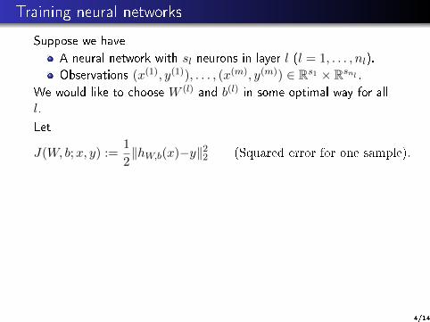
Suppose we have

A neural network with sl neurons in layer l (l = 1, . . . , nl).

Observations (x(1), y(1)), . . . , (x(m), y(m)) ∈ Rs1 × Rsnl .

We would like to choose W (l) and b(l) in some optimal way for all

l.

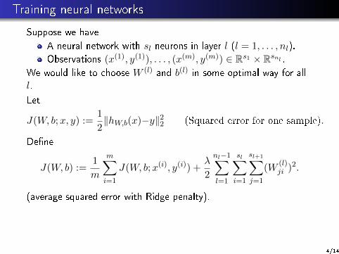
Let

J(W, b;x, y) :=1

2‖hW,b(x)−y‖22 (Squared error for one sample).

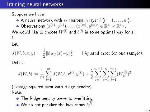
De�ne

J(W, b) :=1

m

m∑i=1

J(W, b;x(i), y(i)) +λ

2

nl−1∑l=1

sl∑i=1

sl+1∑j=1

(W(l)ji )

2.

(average squared error with Ridge penalty).

Note:

The Ridge penalty prevents over�tting.

We do not penalize the bias terms b(l)i .

4/14

Training neural networks

Suppose we have

A neural network with sl neurons in layer l (l = 1, . . . , nl).

Observations (x(1), y(1)), . . . , (x(m), y(m)) ∈ Rs1 × Rsnl .

We would like to choose W (l) and b(l) in some optimal way for all

l.

Let

J(W, b;x, y) :=1

2‖hW,b(x)−y‖22 (Squared error for one sample).

De�ne

J(W, b) :=1

m

m∑i=1

J(W, b;x(i), y(i)) +λ

2

nl−1∑l=1

sl∑i=1

sl+1∑j=1

(W(l)ji )

2.

(average squared error with Ridge penalty).

Note:

The Ridge penalty prevents over�tting.

We do not penalize the bias terms b(l)i .

4/14

Some remarks

Can use other loss functions (e.g. for classi�cation).

Can use other penalties (e.g. `1, elastic net, etc.).

In classi�cation problems, we choose the labels y ∈ {0, 1} (ifworking with sigmoid) or y ∈ {−1, 1} (if working with tanh).

For regression problems, we scale the output so that y ∈ [0, 1](if working with sigmoid) or y ∈ [−1, 1] (if working with tanh).

We can use gradient descent to minimize J(W, b). Note that

since the function J(W, b) is non-convex, we may only �nd a

local minimum.

We need an initial choice for W(l)ij and b

(l)i . If we initialize all

the parameters to 0, then the parameters remain constant over

the layers because of the symmetry of the problem.

As a result, we initialize the parameters to a small constant at

random (say, using N(0, ε2) for ε = 0.01).

5/14

Some remarks

Can use other loss functions (e.g. for classi�cation).

Can use other penalties (e.g. `1, elastic net, etc.).

In classi�cation problems, we choose the labels y ∈ {0, 1} (ifworking with sigmoid) or y ∈ {−1, 1} (if working with tanh).

For regression problems, we scale the output so that y ∈ [0, 1](if working with sigmoid) or y ∈ [−1, 1] (if working with tanh).

We can use gradient descent to minimize J(W, b). Note that

since the function J(W, b) is non-convex, we may only �nd a

local minimum.

We need an initial choice for W(l)ij and b

(l)i . If we initialize all

the parameters to 0, then the parameters remain constant over

the layers because of the symmetry of the problem.

As a result, we initialize the parameters to a small constant at

random (say, using N(0, ε2) for ε = 0.01).

5/14

Some remarks

Can use other loss functions (e.g. for classi�cation).

Can use other penalties (e.g. `1, elastic net, etc.).

In classi�cation problems, we choose the labels y ∈ {0, 1} (ifworking with sigmoid) or y ∈ {−1, 1} (if working with tanh).

For regression problems, we scale the output so that y ∈ [0, 1](if working with sigmoid) or y ∈ [−1, 1] (if working with tanh).

We can use gradient descent to minimize J(W, b). Note that

since the function J(W, b) is non-convex, we may only �nd a

local minimum.

We need an initial choice for W(l)ij and b

(l)i . If we initialize all

the parameters to 0, then the parameters remain constant over

the layers because of the symmetry of the problem.

As a result, we initialize the parameters to a small constant at

random (say, using N(0, ε2) for ε = 0.01).

5/14

Some remarks

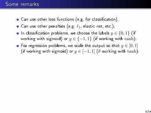
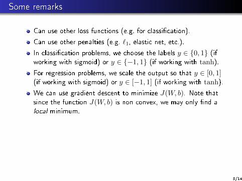
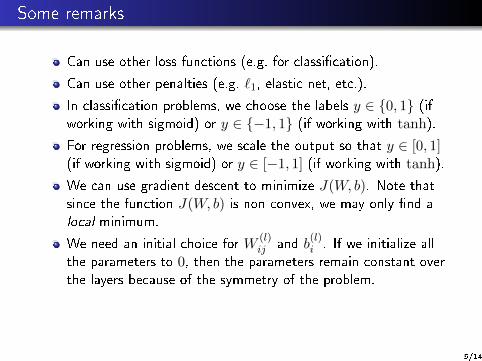
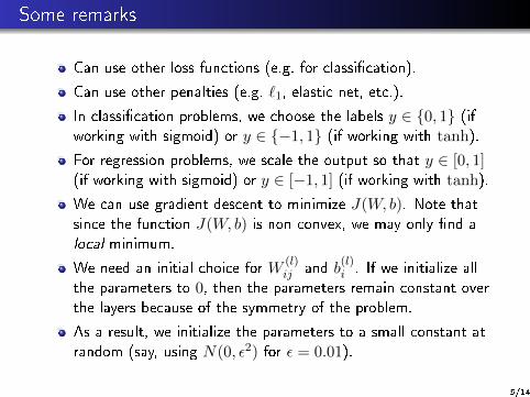
Can use other loss functions (e.g. for classi�cation).

Can use other penalties (e.g. `1, elastic net, etc.).

In classi�cation problems, we choose the labels y ∈ {0, 1} (ifworking with sigmoid) or y ∈ {−1, 1} (if working with tanh).

For regression problems, we scale the output so that y ∈ [0, 1](if working with sigmoid) or y ∈ [−1, 1] (if working with tanh).

We can use gradient descent to minimize J(W, b). Note that

since the function J(W, b) is non-convex, we may only �nd a

local minimum.

We need an initial choice for W(l)ij and b

(l)i . If we initialize all

the parameters to 0, then the parameters remain constant over

the layers because of the symmetry of the problem.

As a result, we initialize the parameters to a small constant at

random (say, using N(0, ε2) for ε = 0.01).

5/14

Some remarks

Can use other loss functions (e.g. for classi�cation).

Can use other penalties (e.g. `1, elastic net, etc.).

In classi�cation problems, we choose the labels y ∈ {0, 1} (ifworking with sigmoid) or y ∈ {−1, 1} (if working with tanh).

For regression problems, we scale the output so that y ∈ [0, 1](if working with sigmoid) or y ∈ [−1, 1] (if working with tanh).

We can use gradient descent to minimize J(W, b). Note that

since the function J(W, b) is non-convex, we may only �nd a

local minimum.

We need an initial choice for W(l)ij and b

(l)i . If we initialize all

the parameters to 0, then the parameters remain constant over

the layers because of the symmetry of the problem.

As a result, we initialize the parameters to a small constant at

random (say, using N(0, ε2) for ε = 0.01).

5/14

Gradient descent and the backpropagation algorithm

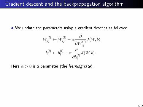
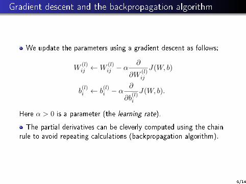
We update the parameters using a gradient descent as follows:

W(l)ij ←W

(l)ij − α

∂

∂W(l)ij

J(W, b)

b(l)i ← b

(l)i − α

∂

∂b(l)i

J(W, b).

Here α > 0 is a parameter (the learning rate).

The partial derivatives can be cleverly computed using the chain

rule to avoid repeating calculations (backpropagation algorithm).

6/14

Gradient descent and the backpropagation algorithm

We update the parameters using a gradient descent as follows:

W(l)ij ←W

(l)ij − α

∂

∂W(l)ij

J(W, b)

b(l)i ← b

(l)i − α

∂

∂b(l)i

J(W, b).

Here α > 0 is a parameter (the learning rate).

The partial derivatives can be cleverly computed using the chain

rule to avoid repeating calculations (backpropagation algorithm).

6/14

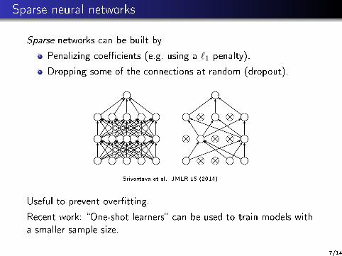
Sparse neural networks

Sparse networks can be built by

Penalizing coe�cients (e.g. using a `1 penalty).

Dropping some of the connections at random (dropout).

Srivastava et al., JMLR 15 (2014).

Useful to prevent over�tting.

Recent work: �One-shot learners� can be used to train models with

a smaller sample size.

7/14

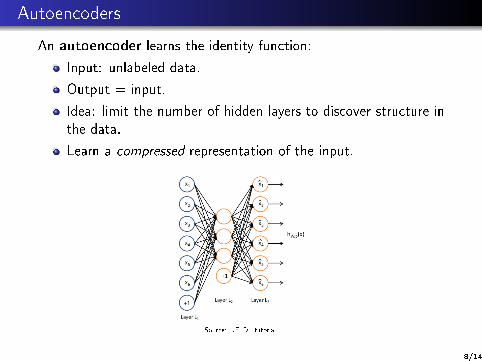
Autoencoders

An autoencoder learns the identity function:

Input: unlabeled data.

Output = input.

Idea: limit the number of hidden layers to discover structure in

the data.

Learn a compressed representation of the input.

Source: UFLDL tutorial.

8/14

Example (UFLDL)

Train an autoencoder on 10× 10 images with one hidden layer.

Each hidden unit i computes:

a(2)i = f

100∑j=1

W(1)ij xj + b

(1)j

.

Think of a(2)i as some non-linear feature of the input x.

Problem: Find x that maximally activates a(2)i over ‖x‖2 ≤ 1.

Claim:

xj =W

(1)ij√∑100

j=1(W(1)ij )2

.

(Hint: Use Cauchy�Schwarz).

We can now display the image maximizing a(2)i for each i.

9/14

Example (UFLDL)

Train an autoencoder on 10× 10 images with one hidden layer.

Each hidden unit i computes:

a(2)i = f

100∑j=1

W(1)ij xj + b

(1)j

.

Think of a(2)i as some non-linear feature of the input x.

Problem: Find x that maximally activates a(2)i over ‖x‖2 ≤ 1.

Claim:

xj =W

(1)ij√∑100

j=1(W(1)ij )2

.

(Hint: Use Cauchy�Schwarz).

We can now display the image maximizing a(2)i for each i.

9/14

Example (UFLDL)

Train an autoencoder on 10× 10 images with one hidden layer.

Each hidden unit i computes:

a(2)i = f

100∑j=1

W(1)ij xj + b

(1)j

.

Think of a(2)i as some non-linear feature of the input x.

Problem: Find x that maximally activates a(2)i over ‖x‖2 ≤ 1.

Claim:

xj =W

(1)ij√∑100

j=1(W(1)ij )2

.

(Hint: Use Cauchy�Schwarz).

We can now display the image maximizing a(2)i for each i.

9/14

Example (UFLDL)

Train an autoencoder on 10× 10 images with one hidden layer.

Each hidden unit i computes:

a(2)i = f

100∑j=1

W(1)ij xj + b

(1)j

.

Think of a(2)i as some non-linear feature of the input x.

Problem: Find x that maximally activates a(2)i over ‖x‖2 ≤ 1.

Claim:

xj =W

(1)ij√∑100

j=1(W(1)ij )2

.

(Hint: Use Cauchy�Schwarz).

We can now display the image maximizing a(2)i for each i.

9/14

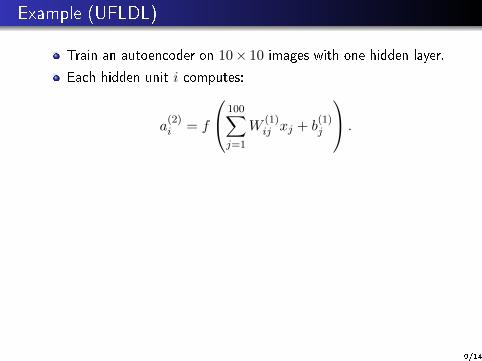
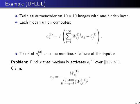
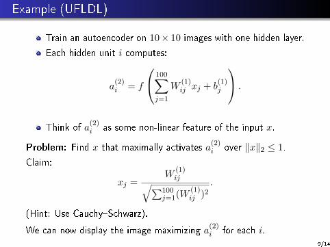
Example (UFLDL)

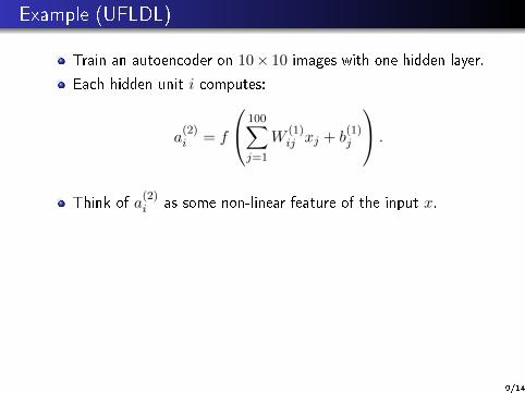
Train an autoencoder on 10× 10 images with one hidden layer.

Each hidden unit i computes:

a(2)i = f

100∑j=1

W(1)ij xj + b

(1)j

.

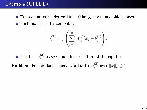
Think of a(2)i as some non-linear feature of the input x.

Problem: Find x that maximally activates a(2)i over ‖x‖2 ≤ 1.

Claim:

xj =W

(1)ij√∑100

j=1(W(1)ij )2

.

(Hint: Use Cauchy�Schwarz).

We can now display the image maximizing a(2)i for each i.

9/14

Example (UFLDL)

Train an autoencoder on 10× 10 images with one hidden layer.

Each hidden unit i computes:

a(2)i = f

100∑j=1

W(1)ij xj + b

(1)j

.

Think of a(2)i as some non-linear feature of the input x.

Problem: Find x that maximally activates a(2)i over ‖x‖2 ≤ 1.

Claim:

xj =W

(1)ij√∑100

j=1(W(1)ij )2

.

(Hint: Use Cauchy�Schwarz).

We can now display the image maximizing a(2)i for each i.

9/14

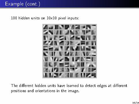
Example (cont.)

100 hidden units on 10x10 pixel inputs:

The di�erent hidden units have learned to detect edges at di�erent

positions and orientations in the image.

10/14

Using convolutions

Idea: Certain signals are stationary, i.e., their statistical

properties do not change in space or time.

For example, images often have similar statistical properties in

di�erent regions in space.

That suggests that the features that we learn at one part of an

image can also be applied to other parts of the image.

Can �convolve� the learned features with the larger image.

Example: 96× 96 image.

Learn features on small 8× 8 patches sampled randomly (e.g.

using a sparse autoencoder).

Run the trained model through all 8× 8 patches of the image

to get the feature activations.

Source: UFLDL tutorial.

11/14

Using convolutions

Idea: Certain signals are stationary, i.e., their statistical

properties do not change in space or time.

For example, images often have similar statistical properties in

di�erent regions in space.

That suggests that the features that we learn at one part of an

image can also be applied to other parts of the image.

Can �convolve� the learned features with the larger image.

Example: 96× 96 image.

Learn features on small 8× 8 patches sampled randomly (e.g.

using a sparse autoencoder).

Run the trained model through all 8× 8 patches of the image

to get the feature activations.

Source: UFLDL tutorial.

11/14

Using convolutions

Idea: Certain signals are stationary, i.e., their statistical

properties do not change in space or time.

For example, images often have similar statistical properties in

di�erent regions in space.

That suggests that the features that we learn at one part of an

image can also be applied to other parts of the image.

Can �convolve� the learned features with the larger image.

Example: 96× 96 image.

Learn features on small 8× 8 patches sampled randomly (e.g.

using a sparse autoencoder).

Run the trained model through all 8× 8 patches of the image

to get the feature activations.

Source: UFLDL tutorial.

11/14

Using convolutions

Idea: Certain signals are stationary, i.e., their statistical

properties do not change in space or time.

For example, images often have similar statistical properties in

di�erent regions in space.

That suggests that the features that we learn at one part of an

image can also be applied to other parts of the image.

Can �convolve� the learned features with the larger image.

Example: 96× 96 image.

Learn features on small 8× 8 patches sampled randomly (e.g.

using a sparse autoencoder).

Run the trained model through all 8× 8 patches of the image

to get the feature activations.

Source: UFLDL tutorial.

11/14

Using convolutions

Idea: Certain signals are stationary, i.e., their statistical

properties do not change in space or time.

For example, images often have similar statistical properties in

di�erent regions in space.

That suggests that the features that we learn at one part of an

image can also be applied to other parts of the image.

Can �convolve� the learned features with the larger image.

Example: 96× 96 image.

Learn features on small 8× 8 patches sampled randomly (e.g.

using a sparse autoencoder).

Run the trained model through all 8× 8 patches of the image

to get the feature activations.

Source: UFLDL tutorial.

11/14

Using convolutions

Idea: Certain signals are stationary, i.e., their statistical

properties do not change in space or time.

For example, images often have similar statistical properties in

di�erent regions in space.

That suggests that the features that we learn at one part of an

image can also be applied to other parts of the image.

Can �convolve� the learned features with the larger image.

Example: 96× 96 image.

Learn features on small 8× 8 patches sampled randomly (e.g.

using a sparse autoencoder).

Run the trained model through all 8× 8 patches of the image

to get the feature activations.

Source: UFLDL tutorial.

11/14

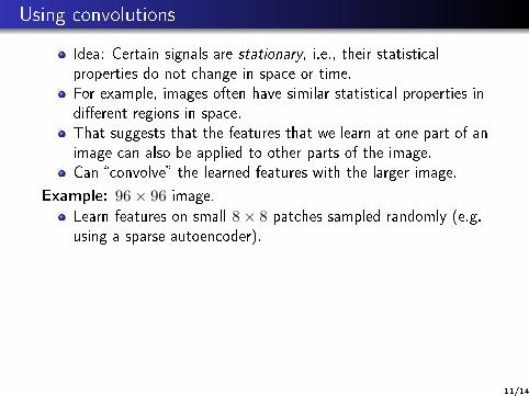
Using convolutions

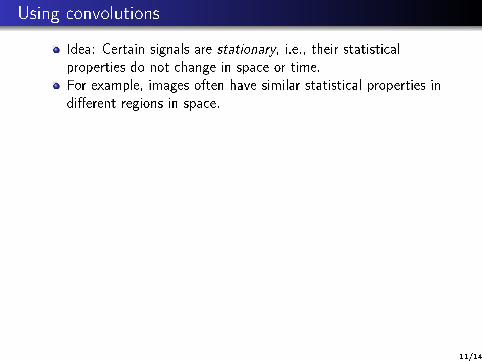
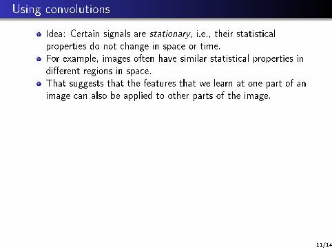
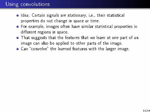
Idea: Certain signals are stationary, i.e., their statistical

properties do not change in space or time.

For example, images often have similar statistical properties in

di�erent regions in space.

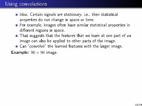
That suggests that the features that we learn at one part of an

image can also be applied to other parts of the image.

Can �convolve� the learned features with the larger image.

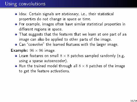
Example: 96× 96 image.

Learn features on small 8× 8 patches sampled randomly (e.g.

using a sparse autoencoder).

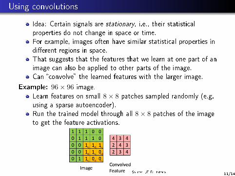
Run the trained model through all 8× 8 patches of the image

to get the feature activations.

Source: UFLDL tutorial.

11/14

Using convolutions

Idea: Certain signals are stationary, i.e., their statistical

properties do not change in space or time.

For example, images often have similar statistical properties in

di�erent regions in space.

That suggests that the features that we learn at one part of an

image can also be applied to other parts of the image.

Can �convolve� the learned features with the larger image.

Example: 96× 96 image.

Learn features on small 8× 8 patches sampled randomly (e.g.

using a sparse autoencoder).

Run the trained model through all 8× 8 patches of the image

to get the feature activations.

Source: UFLDL tutorial. 11/14

Pooling features

Once can also pool the features obtained via convolution.

For example, to describe a large image, one natural approach

is to aggregate statistics of these features at various locations.

E.g. compute the mean, max, etc. over di�erent regions.

Can lead to more robust features. Can lead to invariant

features.

For example, if the pooling regions are contiguous, then the

pooling units will be �translation invariant�, i.e., they won't

change much if objects in the image are undergo a (small)

translation.

12/14

Pooling features

Once can also pool the features obtained via convolution.

For example, to describe a large image, one natural approach

is to aggregate statistics of these features at various locations.

E.g. compute the mean, max, etc. over di�erent regions.

Can lead to more robust features. Can lead to invariant

features.

For example, if the pooling regions are contiguous, then the

pooling units will be �translation invariant�, i.e., they won't

change much if objects in the image are undergo a (small)

translation.

12/14

Pooling features

Once can also pool the features obtained via convolution.

For example, to describe a large image, one natural approach

is to aggregate statistics of these features at various locations.

E.g. compute the mean, max, etc. over di�erent regions.

Can lead to more robust features. Can lead to invariant

features.

For example, if the pooling regions are contiguous, then the

pooling units will be �translation invariant�, i.e., they won't

change much if objects in the image are undergo a (small)

translation.

12/14

Pooling features

Once can also pool the features obtained via convolution.

For example, to describe a large image, one natural approach

is to aggregate statistics of these features at various locations.

E.g. compute the mean, max, etc. over di�erent regions.

Can lead to more robust features. Can lead to invariant

features.

For example, if the pooling regions are contiguous, then the

pooling units will be �translation invariant�, i.e., they won't

change much if objects in the image are undergo a (small)

translation.

12/14

Pooling features

Once can also pool the features obtained via convolution.

For example, to describe a large image, one natural approach

is to aggregate statistics of these features at various locations.

E.g. compute the mean, max, etc. over di�erent regions.

Can lead to more robust features. Can lead to invariant

features.

For example, if the pooling regions are contiguous, then the

pooling units will be �translation invariant�, i.e., they won't

change much if objects in the image are undergo a (small)

translation.

12/14

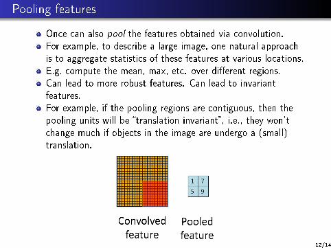
Pooling features

Once can also pool the features obtained via convolution.

For example, to describe a large image, one natural approach

is to aggregate statistics of these features at various locations.

E.g. compute the mean, max, etc. over di�erent regions.

Can lead to more robust features. Can lead to invariant

features.

For example, if the pooling regions are contiguous, then the

pooling units will be �translation invariant�, i.e., they won't

change much if objects in the image are undergo a (small)

translation.

12/14

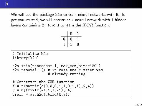
R

We will use the package h2o to train neural networks with R. To

get you started, we will construct a neural network with 1 hidden

layers containing 2 neurons to learn the XOR function:

0 1

0 0 1

1 1 0

# Initialize h2olibrary(h2o)

h2o.init(nthreads=-1, max_mem_size="2G")h2o.removeAll() # in case the cluster was

# already running

# Construct the XOR functionX = t(matrix(c(0,0,0,1,1,0,1,1),2,4))y = matrix(c(-1,1,1,-1), 4)train = as.h2o(cbind(X,y))

13/14

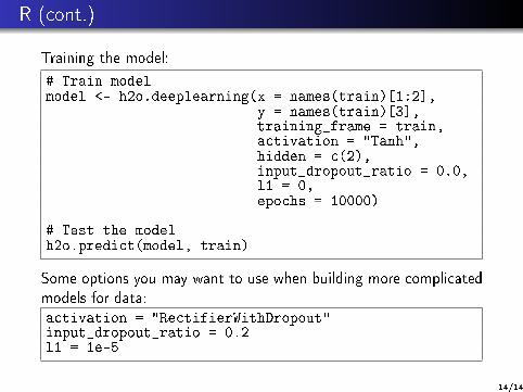
R (cont.)

Training the model:

# Train modelmodel <- h2o.deeplearning(x = names(train)[1:2],

y = names(train)[3],training_frame = train,activation = "Tanh",hidden = c(2),input_dropout_ratio = 0.0,l1 = 0,epochs = 10000)

# Test the modelh2o.predict(model, train)

Some options you may want to use when building more complicated

models for data:activation = "RectifierWithDropout"input_dropout_ratio = 0.2l1 = 1e-5

14/14