Embed Size (px)
Citation preview
MATH 590: Meshfree MethodsChapter 43: RBF-PS Methods in MATLAB
Greg Fasshauer
Department of Applied MathematicsIllinois Institute of Technology
Fall 2010
[email protected] MATH 590 – Chapter 43 1
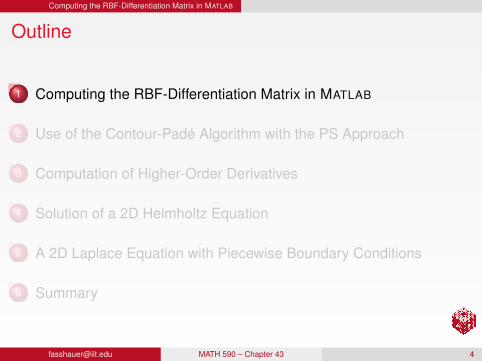
Outline
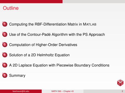
1 Computing the RBF-Differentiation Matrix in MATLAB
2 Use of the Contour-Padé Algorithm with the PS Approach
3 Computation of Higher-Order Derivatives
4 Solution of a 2D Helmholtz Equation
5 A 2D Laplace Equation with Piecewise Boundary Conditions
6 Summary
[email protected] MATH 590 – Chapter 43 2
The coupling of RBF collocation and pseudospectral methodsdiscussed in the previous chapter has provided a number of newinsights.
We can apply many standard pseudospectral procedures to RBFsolvers.In particular, we now have “standard” procedures for solvingtime-dependent PDEs with RBFs.
In this chapter we illustrate how the RBF pseudospectral approach canbe applied in a way very similar to standard polynomial pseudospectralmethods.Among our numerical illustrations are several examples taken from thebook [Trefethen (2000)] (see Programs 17, 35 and 36 there).We will also use the 1D transport equation from the previous chapterto compare the RBF and polynomial PS methods.
[email protected] MATH 590 – Chapter 43 3
The coupling of RBF collocation and pseudospectral methodsdiscussed in the previous chapter has provided a number of newinsights.
We can apply many standard pseudospectral procedures to RBFsolvers.
In particular, we now have “standard” procedures for solvingtime-dependent PDEs with RBFs.
In this chapter we illustrate how the RBF pseudospectral approach canbe applied in a way very similar to standard polynomial pseudospectralmethods.Among our numerical illustrations are several examples taken from thebook [Trefethen (2000)] (see Programs 17, 35 and 36 there).We will also use the 1D transport equation from the previous chapterto compare the RBF and polynomial PS methods.
[email protected] MATH 590 – Chapter 43 3
The coupling of RBF collocation and pseudospectral methodsdiscussed in the previous chapter has provided a number of newinsights.
We can apply many standard pseudospectral procedures to RBFsolvers.In particular, we now have “standard” procedures for solvingtime-dependent PDEs with RBFs.
In this chapter we illustrate how the RBF pseudospectral approach canbe applied in a way very similar to standard polynomial pseudospectralmethods.Among our numerical illustrations are several examples taken from thebook [Trefethen (2000)] (see Programs 17, 35 and 36 there).We will also use the 1D transport equation from the previous chapterto compare the RBF and polynomial PS methods.
[email protected] MATH 590 – Chapter 43 3
The coupling of RBF collocation and pseudospectral methodsdiscussed in the previous chapter has provided a number of newinsights.
We can apply many standard pseudospectral procedures to RBFsolvers.In particular, we now have “standard” procedures for solvingtime-dependent PDEs with RBFs.
In this chapter we illustrate how the RBF pseudospectral approach canbe applied in a way very similar to standard polynomial pseudospectralmethods.
Among our numerical illustrations are several examples taken from thebook [Trefethen (2000)] (see Programs 17, 35 and 36 there).We will also use the 1D transport equation from the previous chapterto compare the RBF and polynomial PS methods.
[email protected] MATH 590 – Chapter 43 3
The coupling of RBF collocation and pseudospectral methodsdiscussed in the previous chapter has provided a number of newinsights.
We can apply many standard pseudospectral procedures to RBFsolvers.In particular, we now have “standard” procedures for solvingtime-dependent PDEs with RBFs.
In this chapter we illustrate how the RBF pseudospectral approach canbe applied in a way very similar to standard polynomial pseudospectralmethods.Among our numerical illustrations are several examples taken from thebook [Trefethen (2000)] (see Programs 17, 35 and 36 there).
We will also use the 1D transport equation from the previous chapterto compare the RBF and polynomial PS methods.
[email protected] MATH 590 – Chapter 43 3
The coupling of RBF collocation and pseudospectral methodsdiscussed in the previous chapter has provided a number of newinsights.
We can apply many standard pseudospectral procedures to RBFsolvers.In particular, we now have “standard” procedures for solvingtime-dependent PDEs with RBFs.
In this chapter we illustrate how the RBF pseudospectral approach canbe applied in a way very similar to standard polynomial pseudospectralmethods.Among our numerical illustrations are several examples taken from thebook [Trefethen (2000)] (see Programs 17, 35 and 36 there).We will also use the 1D transport equation from the previous chapterto compare the RBF and polynomial PS methods.
[email protected] MATH 590 – Chapter 43 3
Computing the RBF-Differentiation Matrix in MATLAB
Outline
1 Computing the RBF-Differentiation Matrix in MATLAB
2 Use of the Contour-Padé Algorithm with the PS Approach
3 Computation of Higher-Order Derivatives
4 Solution of a 2D Helmholtz Equation
5 A 2D Laplace Equation with Piecewise Boundary Conditions
6 Summary
[email protected] MATH 590 – Chapter 43 4
Computing the RBF-Differentiation Matrix in MATLAB
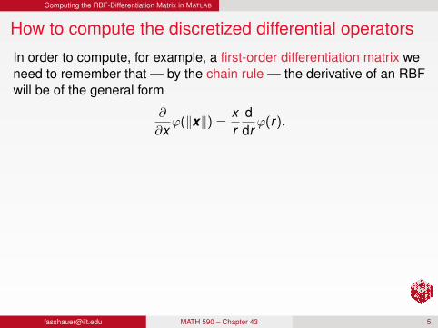
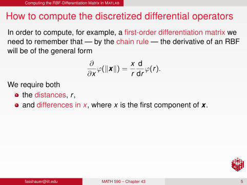
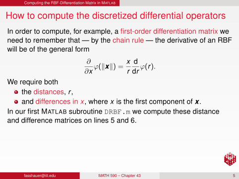
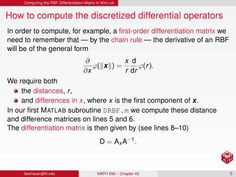
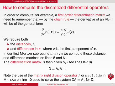
How to compute the discretized differential operators
In order to compute, for example, a first-order differentiation matrix weneed to remember that — by the chain rule — the derivative of an RBFwill be of the general form
∂
∂xϕ(‖x‖) =
xr
ddrϕ(r).
We require boththe distances, r ,and differences in x , where x is the first component of x .
In our first MATLAB subroutine DRBF.m we compute these distanceand difference matrices on lines 5 and 6.The differentiation matrix is then given by (see lines 8–10)
D = AxA−1.
Note the use of the matrix right division operator / or mrdivide inMATLAB on line 10 used to solve the system DA = Ax for D.
[email protected] MATH 590 – Chapter 43 5
Computing the RBF-Differentiation Matrix in MATLAB
How to compute the discretized differential operators
In order to compute, for example, a first-order differentiation matrix weneed to remember that — by the chain rule — the derivative of an RBFwill be of the general form
∂
∂xϕ(‖x‖) =
xr
ddrϕ(r).
We require boththe distances, r ,and differences in x , where x is the first component of x .
In our first MATLAB subroutine DRBF.m we compute these distanceand difference matrices on lines 5 and 6.
The differentiation matrix is then given by (see lines 8–10)
D = AxA−1.
Note the use of the matrix right division operator / or mrdivide inMATLAB on line 10 used to solve the system DA = Ax for D.
[email protected] MATH 590 – Chapter 43 5
Computing the RBF-Differentiation Matrix in MATLAB
How to compute the discretized differential operators
In order to compute, for example, a first-order differentiation matrix weneed to remember that — by the chain rule — the derivative of an RBFwill be of the general form
∂
∂xϕ(‖x‖) =
xr
ddrϕ(r).
We require boththe distances, r ,and differences in x , where x is the first component of x .
In our first MATLAB subroutine DRBF.m we compute these distanceand difference matrices on lines 5 and 6.The differentiation matrix is then given by (see lines 8–10)
D = AxA−1.
Note the use of the matrix right division operator / or mrdivide inMATLAB on line 10 used to solve the system DA = Ax for D.
[email protected] MATH 590 – Chapter 43 5
Computing the RBF-Differentiation Matrix in MATLAB
How to compute the discretized differential operators
In order to compute, for example, a first-order differentiation matrix weneed to remember that — by the chain rule — the derivative of an RBFwill be of the general form
∂
∂xϕ(‖x‖) =
xr
ddrϕ(r).
We require boththe distances, r ,and differences in x , where x is the first component of x .
In our first MATLAB subroutine DRBF.m we compute these distanceand difference matrices on lines 5 and 6.The differentiation matrix is then given by (see lines 8–10)
D = AxA−1.
Note the use of the matrix right division operator / or mrdivide inMATLAB on line 10 used to solve the system DA = Ax for D.
[email protected] MATH 590 – Chapter 43 5
Computing the RBF-Differentiation Matrix in MATLAB
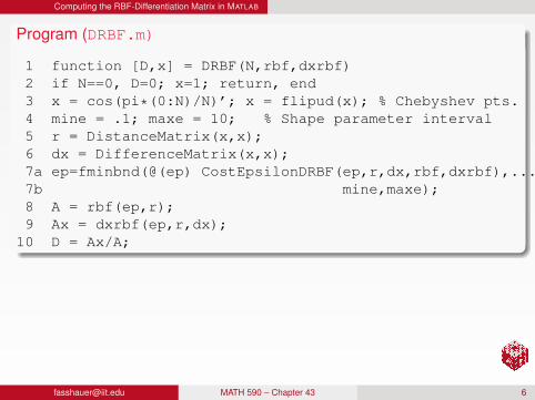
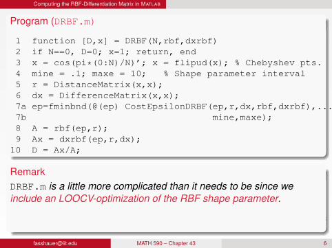
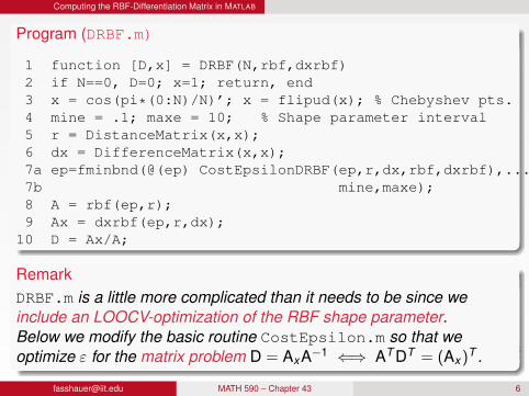
Program (DRBF.m)
1 function [D,x] = DRBF(N,rbf,dxrbf)2 if N==0, D=0; x=1; return, end3 x = cos(pi*(0:N)/N)’; x = flipud(x); % Chebyshev pts.4 mine = .1; maxe = 10; % Shape parameter interval5 r = DistanceMatrix(x,x);6 dx = DifferenceMatrix(x,x);7a ep=fminbnd(@(ep) CostEpsilonDRBF(ep,r,dx,rbf,dxrbf),...7b mine,maxe);8 A = rbf(ep,r);9 Ax = dxrbf(ep,r,dx);
10 D = Ax/A;
RemarkDRBF.m is a little more complicated than it needs to be since weinclude an LOOCV-optimization of the RBF shape parameter.Below we modify the basic routine CostEpsilon.m so that weoptimize ε for the matrix problem D = AxA−1 ⇐⇒ AT DT = (Ax )T .
[email protected] MATH 590 – Chapter 43 6
Computing the RBF-Differentiation Matrix in MATLAB
Program (DRBF.m)
1 function [D,x] = DRBF(N,rbf,dxrbf)2 if N==0, D=0; x=1; return, end3 x = cos(pi*(0:N)/N)’; x = flipud(x); % Chebyshev pts.4 mine = .1; maxe = 10; % Shape parameter interval5 r = DistanceMatrix(x,x);6 dx = DifferenceMatrix(x,x);7a ep=fminbnd(@(ep) CostEpsilonDRBF(ep,r,dx,rbf,dxrbf),...7b mine,maxe);8 A = rbf(ep,r);9 Ax = dxrbf(ep,r,dx);
10 D = Ax/A;
RemarkDRBF.m is a little more complicated than it needs to be since weinclude an LOOCV-optimization of the RBF shape parameter.
Below we modify the basic routine CostEpsilon.m so that weoptimize ε for the matrix problem D = AxA−1 ⇐⇒ AT DT = (Ax )T .
[email protected] MATH 590 – Chapter 43 6
Computing the RBF-Differentiation Matrix in MATLAB
Program (DRBF.m)
1 function [D,x] = DRBF(N,rbf,dxrbf)2 if N==0, D=0; x=1; return, end3 x = cos(pi*(0:N)/N)’; x = flipud(x); % Chebyshev pts.4 mine = .1; maxe = 10; % Shape parameter interval5 r = DistanceMatrix(x,x);6 dx = DifferenceMatrix(x,x);7a ep=fminbnd(@(ep) CostEpsilonDRBF(ep,r,dx,rbf,dxrbf),...7b mine,maxe);8 A = rbf(ep,r);9 Ax = dxrbf(ep,r,dx);
10 D = Ax/A;
RemarkDRBF.m is a little more complicated than it needs to be since weinclude an LOOCV-optimization of the RBF shape parameter.Below we modify the basic routine CostEpsilon.m so that weoptimize ε for the matrix problem D = AxA−1 ⇐⇒ AT DT = (Ax )T .
[email protected] MATH 590 – Chapter 43 6
Computing the RBF-Differentiation Matrix in MATLAB
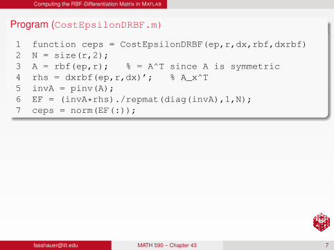
Program (CostEpsilonDRBF.m)
1 function ceps = CostEpsilonDRBF(ep,r,dx,rbf,dxrbf)2 N = size(r,2);3 A = rbf(ep,r); % = A^T since A is symmetric4 rhs = dxrbf(ep,r,dx)’; % A_x^T5 invA = pinv(A);6 EF = (invA*rhs)./repmat(diag(invA),1,N);7 ceps = norm(EF(:));
RemarkNote that CostEpsilonDRBF.m is very similar to CostEpsilon.m.Now, however, we compute a right-hand side matrix corresponding tothe transpose of Ax .Therefore, the denominator — which remains the same for allright-hand sides — needs to be cloned on line 6 via the repmatcommand.The cost of ε is now the Frobenius norm of the matrix EF.
[email protected] MATH 590 – Chapter 43 7
Computing the RBF-Differentiation Matrix in MATLAB
Program (CostEpsilonDRBF.m)
1 function ceps = CostEpsilonDRBF(ep,r,dx,rbf,dxrbf)2 N = size(r,2);3 A = rbf(ep,r); % = A^T since A is symmetric4 rhs = dxrbf(ep,r,dx)’; % A_x^T5 invA = pinv(A);6 EF = (invA*rhs)./repmat(diag(invA),1,N);7 ceps = norm(EF(:));
RemarkNote that CostEpsilonDRBF.m is very similar to CostEpsilon.m.Now, however, we compute a right-hand side matrix corresponding tothe transpose of Ax .Therefore, the denominator — which remains the same for allright-hand sides — needs to be cloned on line 6 via the repmatcommand.The cost of ε is now the Frobenius norm of the matrix EF.
[email protected] MATH 590 – Chapter 43 7
Computing the RBF-Differentiation Matrix in MATLAB Solution of a 1-D Transport Equation
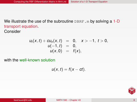
We illustrate the use of the subroutine DBRF.m by solving a 1-Dtransport equation.Consider
ut (x , t) + cux (x , t) = 0, x > −1, t > 0,u(−1, t) = 0,u(x ,0) = f (x),
with the well-known solution
u(x , t) = f (x − ct).
[email protected] MATH 590 – Chapter 43 8
Computing the RBF-Differentiation Matrix in MATLAB Solution of a 1-D Transport Equation
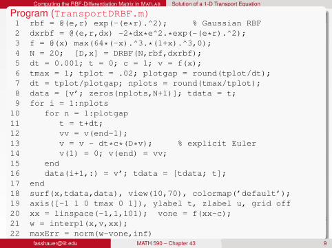
Program (TransportDRBF.m)1 rbf = @(e,r) exp(-(e*r).^2); % Gaussian RBF2 dxrbf = @(e,r,dx) -2*dx*e^2.*exp(-(e*r).^2);3 f = @(x) max(64*(-x).^3.*(1+x).^3,0);4 N = 20; [D,x] = DRBF(N,rbf,dxrbf);5 dt = 0.001; t = 0; c = 1; v = f(x);6 tmax = 1; tplot = .02; plotgap = round(tplot/dt);7 dt = tplot/plotgap; nplots = round(tmax/tplot);8 data = [v’; zeros(nplots,N+1)]; tdata = t;9 for i = 1:nplots
10 for n = 1:plotgap11 t = t+dt;12 vv = v(end-1);13 v = v - dt*c*(D*v); % explicit Euler14 v(1) = 0; v(end) = vv;15 end16 data(i+1,:) = v’; tdata = [tdata; t];17 end18 surf(x,tdata,data), view(10,70), colormap(’default’);19 axis([-1 1 0 tmax 0 1]), ylabel t, zlabel u, grid off20 xx = linspace(-1,1,101); vone = f(xx-c);21 w = interp1(x,v,xx);22 maxErr = norm(w-vone,inf)
[email protected] MATH 590 – Chapter 43 9
Computing the RBF-Differentiation Matrix in MATLAB Solution of a 1-D Transport Equation
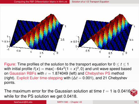
Figure: Time profiles of the solution to the transport equation for 0 ≤ t ≤ 1with initial profile f (x) = max(−64x3(1 + x)3,0) and unit wave speed basedon Gaussian RBFs with ε = 1.874049 (left) and Chebyshev PS method(right). Explicit Euler time-stepping with (∆t = 0.001), and 21 Chebyshevpoints.
The maximum error for the Gaussian solution at time t = 1 is 0.0416,while for the PS solution we get 0.0418.
[email protected] MATH 590 – Chapter 43 10
Computing the RBF-Differentiation Matrix in MATLAB Solution of a 1-D Transport Equation
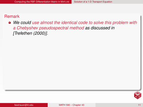
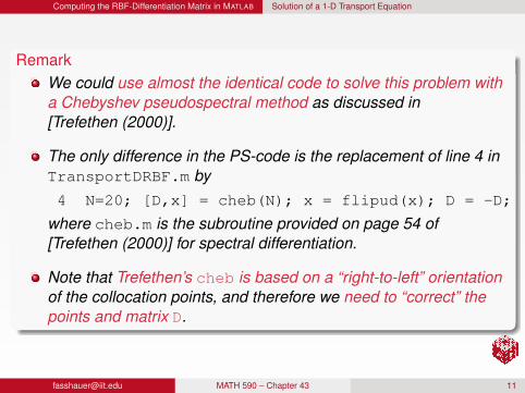
RemarkWe could use almost the identical code to solve this problem witha Chebyshev pseudospectral method as discussed in[Trefethen (2000)].
The only difference in the PS-code is the replacement of line 4 inTransportDRBF.m by4 N=20; [D,x] = cheb(N); x = flipud(x); D = -D;
where cheb.m is the subroutine provided on page 54 of[Trefethen (2000)] for spectral differentiation.
Note that Trefethen’s cheb is based on a “right-to-left” orientationof the collocation points, and therefore we need to “correct” thepoints and matrix D.
[email protected] MATH 590 – Chapter 43 11
Computing the RBF-Differentiation Matrix in MATLAB Solution of a 1-D Transport Equation
RemarkWe could use almost the identical code to solve this problem witha Chebyshev pseudospectral method as discussed in[Trefethen (2000)].
The only difference in the PS-code is the replacement of line 4 inTransportDRBF.m by4 N=20; [D,x] = cheb(N); x = flipud(x); D = -D;
where cheb.m is the subroutine provided on page 54 of[Trefethen (2000)] for spectral differentiation.
Note that Trefethen’s cheb is based on a “right-to-left” orientationof the collocation points, and therefore we need to “correct” thepoints and matrix D.
[email protected] MATH 590 – Chapter 43 11
Use of the Contour-Padé Algorithm with the PS Approach
Outline
1 Computing the RBF-Differentiation Matrix in MATLAB
2 Use of the Contour-Padé Algorithm with the PS Approach
3 Computation of Higher-Order Derivatives
4 Solution of a 2D Helmholtz Equation
5 A 2D Laplace Equation with Piecewise Boundary Conditions
6 Summary
[email protected] MATH 590 – Chapter 43 12
Use of the Contour-Padé Algorithm with the PS Approach
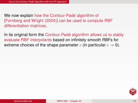
We now explain how the Contour-Padé algorithm of[Fornberg and Wright (2004)] can be used to compute RBFdifferentiation matrices.
In its original form the Contour-Padé algorithm allows us to stablyevaluate RBF interpolants based on infinitely smooth RBFs forextreme choices of the shape parameter ε (in particular ε→ 0).
The Contour-Padé algorithm uses FFTs and Padé approximations toevaluate the function
u(x , ε) = bT (x , ε)(A(ε))−1f (1)
with b(x , ε)j = ϕε(‖x − x j‖) at some evaluation point x andA(ε)i,j = ϕε(‖x i − x j‖).
[email protected] MATH 590 – Chapter 43 13
Use of the Contour-Padé Algorithm with the PS Approach
We now explain how the Contour-Padé algorithm of[Fornberg and Wright (2004)] can be used to compute RBFdifferentiation matrices.
In its original form the Contour-Padé algorithm allows us to stablyevaluate RBF interpolants based on infinitely smooth RBFs forextreme choices of the shape parameter ε (in particular ε→ 0).
The Contour-Padé algorithm uses FFTs and Padé approximations toevaluate the function
u(x , ε) = bT (x , ε)(A(ε))−1f (1)
with b(x , ε)j = ϕε(‖x − x j‖) at some evaluation point x andA(ε)i,j = ϕε(‖x i − x j‖).
[email protected] MATH 590 – Chapter 43 13

Use of the Contour-Padé Algorithm with the PS Approach
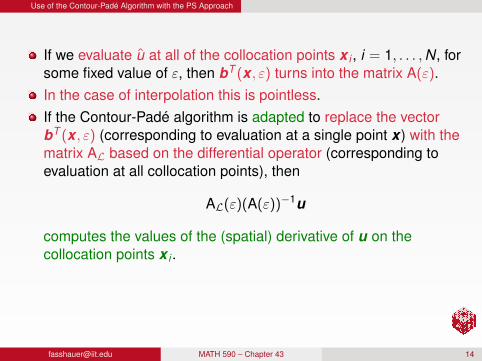
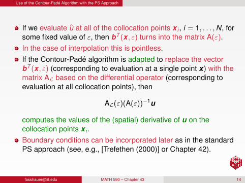
If we evaluate u at all of the collocation points x i , i = 1, . . . ,N, forsome fixed value of ε, then bT (x , ε) turns into the matrix A(ε).
In the case of interpolation this is pointless.If the Contour-Padé algorithm is adapted to replace the vectorbT (x , ε) (corresponding to evaluation at a single point x) with thematrix AL based on the differential operator (corresponding toevaluation at all collocation points), then
AL(ε)(A(ε))−1u
computes the values of the (spatial) derivative of u on thecollocation points x i .Boundary conditions can be incorporated later as in the standardPS approach (see, e.g., [Trefethen (2000)] or Chapter 42).
[email protected] MATH 590 – Chapter 43 14
Use of the Contour-Padé Algorithm with the PS Approach
If we evaluate u at all of the collocation points x i , i = 1, . . . ,N, forsome fixed value of ε, then bT (x , ε) turns into the matrix A(ε).In the case of interpolation this is pointless.
If the Contour-Padé algorithm is adapted to replace the vectorbT (x , ε) (corresponding to evaluation at a single point x) with thematrix AL based on the differential operator (corresponding toevaluation at all collocation points), then
AL(ε)(A(ε))−1u
computes the values of the (spatial) derivative of u on thecollocation points x i .Boundary conditions can be incorporated later as in the standardPS approach (see, e.g., [Trefethen (2000)] or Chapter 42).
[email protected] MATH 590 – Chapter 43 14
Use of the Contour-Padé Algorithm with the PS Approach
If we evaluate u at all of the collocation points x i , i = 1, . . . ,N, forsome fixed value of ε, then bT (x , ε) turns into the matrix A(ε).In the case of interpolation this is pointless.If the Contour-Padé algorithm is adapted to replace the vectorbT (x , ε) (corresponding to evaluation at a single point x) with thematrix AL based on the differential operator (corresponding toevaluation at all collocation points), then
AL(ε)(A(ε))−1u
computes the values of the (spatial) derivative of u on thecollocation points x i .
Boundary conditions can be incorporated later as in the standardPS approach (see, e.g., [Trefethen (2000)] or Chapter 42).
[email protected] MATH 590 – Chapter 43 14
Use of the Contour-Padé Algorithm with the PS Approach
If we evaluate u at all of the collocation points x i , i = 1, . . . ,N, forsome fixed value of ε, then bT (x , ε) turns into the matrix A(ε).In the case of interpolation this is pointless.If the Contour-Padé algorithm is adapted to replace the vectorbT (x , ε) (corresponding to evaluation at a single point x) with thematrix AL based on the differential operator (corresponding toevaluation at all collocation points), then
AL(ε)(A(ε))−1u
computes the values of the (spatial) derivative of u on thecollocation points x i .Boundary conditions can be incorporated later as in the standardPS approach (see, e.g., [Trefethen (2000)] or Chapter 42).
[email protected] MATH 590 – Chapter 43 14

Use of the Contour-Padé Algorithm with the PS Approach Solution of the 1D Transport Equation Revisited
This means that we can add another subroutine to compute thedifferentiation matrix on line 4 of TransportDRBF.m via theContour-Padé algorithm.
We comparea solution based on the Contour-Padé algorithm for Gaussian RBFsin the limiting case ε→ 0to the two methods described earlier (based on DRBF and cheb).
All methods use an implicit Euler method with time step∆t = 0.001 for the time discretization.For an implicit time-stepping method both the Contour-Padéapproach and the DRBF approach require an inversion of thedifferentiation matrix.Recall that our theoretical discussion suggested that this isjustified as long as we’re in the limiting case ε→ 0 and one spacedimension.We will see that the non-limiting case (using DRBF) seems to workjust as well.
[email protected] MATH 590 – Chapter 43 15
Use of the Contour-Padé Algorithm with the PS Approach Solution of the 1D Transport Equation Revisited
This means that we can add another subroutine to compute thedifferentiation matrix on line 4 of TransportDRBF.m via theContour-Padé algorithm.We compare
a solution based on the Contour-Padé algorithm for Gaussian RBFsin the limiting case ε→ 0to the two methods described earlier (based on DRBF and cheb).
All methods use an implicit Euler method with time step∆t = 0.001 for the time discretization.
For an implicit time-stepping method both the Contour-Padéapproach and the DRBF approach require an inversion of thedifferentiation matrix.Recall that our theoretical discussion suggested that this isjustified as long as we’re in the limiting case ε→ 0 and one spacedimension.We will see that the non-limiting case (using DRBF) seems to workjust as well.
[email protected] MATH 590 – Chapter 43 15
Use of the Contour-Padé Algorithm with the PS Approach Solution of the 1D Transport Equation Revisited
This means that we can add another subroutine to compute thedifferentiation matrix on line 4 of TransportDRBF.m via theContour-Padé algorithm.We compare
a solution based on the Contour-Padé algorithm for Gaussian RBFsin the limiting case ε→ 0to the two methods described earlier (based on DRBF and cheb).
All methods use an implicit Euler method with time step∆t = 0.001 for the time discretization.For an implicit time-stepping method both the Contour-Padéapproach and the DRBF approach require an inversion of thedifferentiation matrix.
Recall that our theoretical discussion suggested that this isjustified as long as we’re in the limiting case ε→ 0 and one spacedimension.We will see that the non-limiting case (using DRBF) seems to workjust as well.
[email protected] MATH 590 – Chapter 43 15
Use of the Contour-Padé Algorithm with the PS Approach Solution of the 1D Transport Equation Revisited
This means that we can add another subroutine to compute thedifferentiation matrix on line 4 of TransportDRBF.m via theContour-Padé algorithm.We compare
a solution based on the Contour-Padé algorithm for Gaussian RBFsin the limiting case ε→ 0to the two methods described earlier (based on DRBF and cheb).
All methods use an implicit Euler method with time step∆t = 0.001 for the time discretization.For an implicit time-stepping method both the Contour-Padéapproach and the DRBF approach require an inversion of thedifferentiation matrix.Recall that our theoretical discussion suggested that this isjustified as long as we’re in the limiting case ε→ 0 and one spacedimension.
We will see that the non-limiting case (using DRBF) seems to workjust as well.
[email protected] MATH 590 – Chapter 43 15
Use of the Contour-Padé Algorithm with the PS Approach Solution of the 1D Transport Equation Revisited
This means that we can add another subroutine to compute thedifferentiation matrix on line 4 of TransportDRBF.m via theContour-Padé algorithm.We compare
a solution based on the Contour-Padé algorithm for Gaussian RBFsin the limiting case ε→ 0to the two methods described earlier (based on DRBF and cheb).
All methods use an implicit Euler method with time step∆t = 0.001 for the time discretization.For an implicit time-stepping method both the Contour-Padéapproach and the DRBF approach require an inversion of thedifferentiation matrix.Recall that our theoretical discussion suggested that this isjustified as long as we’re in the limiting case ε→ 0 and one spacedimension.We will see that the non-limiting case (using DRBF) seems to workjust as well.
[email protected] MATH 590 – Chapter 43 15
Use of the Contour-Padé Algorithm with the PS Approach Solution of the 1D Transport Equation Revisited
6 8 10 12 14 16 1810
−2
10−1
100
N
Err
or
6 8 10 12 14 16 1810
−2
10−1
100
N
Err
or
6 8 10 12 14 16 1810
−2
10−1
100
N
Err
or
6 8 10 12 14 16 180
0.2
0.4
0.6
0.8
1
1.2
1.4
1.6
N
Opt
imal
eps
ilon
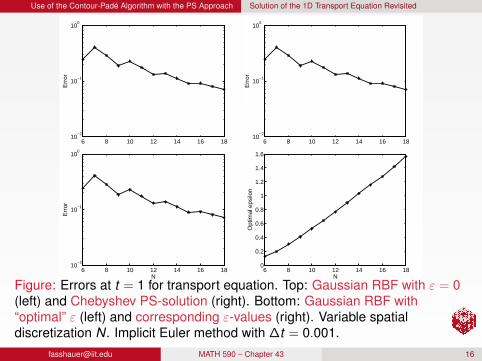
Figure: Errors at t = 1 for transport equation. Top: Gaussian RBF with ε = 0(left) and Chebyshev PS-solution (right). Bottom: Gaussian RBF with“optimal” ε (left) and corresponding ε-values (right). Variable spatialdiscretization N. Implicit Euler method with ∆t = 0.001.
[email protected] MATH 590 – Chapter 43 16
Use of the Contour-Padé Algorithm with the PS Approach Solution of the 1D Transport Equation Revisited
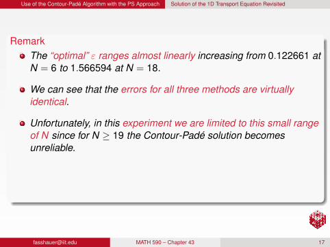
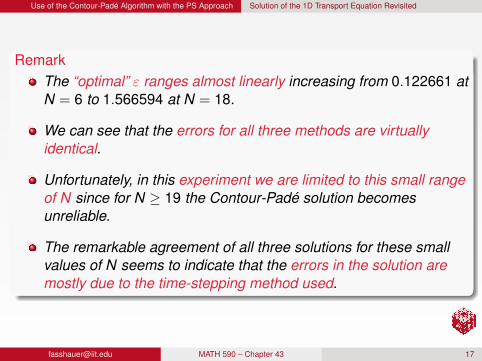
RemarkThe “optimal” ε ranges almost linearly increasing from 0.122661 atN = 6 to 1.566594 at N = 18.
We can see that the errors for all three methods are virtuallyidentical.
Unfortunately, in this experiment we are limited to this small rangeof N since for N ≥ 19 the Contour-Padé solution becomesunreliable.
The remarkable agreement of all three solutions for these smallvalues of N seems to indicate that the errors in the solution aremostly due to the time-stepping method used.
[email protected] MATH 590 – Chapter 43 17
Use of the Contour-Padé Algorithm with the PS Approach Solution of the 1D Transport Equation Revisited
−3 −2 −1 0 1 2 3
x 10−3
−2
−1
0
1
2
x 10−3
Re
Im
−0.2 −0.1 0 0.1 0.2−0.2
−0.15
−0.1
−0.05
0
0.05
0.1
0.15
0.2
Re
Im
−2 −1 0 1 2
−2
−1
0
1
2
Re
Im
−5 0 5 10−8
−6
−4
−2
0
2
4
6
8
Re
Im
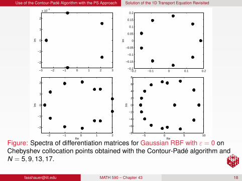
Figure: Spectra of differentiation matrices for Gaussian RBF with ε = 0 onChebyshev collocation points obtained with the Contour-Padé algorithm andN = 5,9,13,17.
[email protected] MATH 590 – Chapter 43 18
Use of the Contour-Padé Algorithm with the PS Approach Solution of the 1D Transport Equation Revisited
−2 −1 0 1 2
x 10−3
−2
−1
0
1
2
x 10−3
Re
Im
−0.2 −0.1 0 0.1 0.2−0.2
−0.15
−0.1
−0.05
0
0.05
0.1
0.15
0.2
Re
Im
−0.8 −0.6 −0.4 −0.2 0 0.2 0.4 0.6−0.8
−0.6
−0.4
−0.2
0
0.2
0.4
0.6
0.8
Re
Im
−2 −1 0 1 2−2
−1.5
−1
−0.5
0
0.5
1
1.5
2
Re
Im
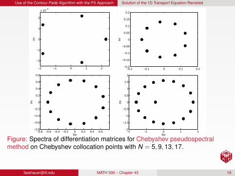
Figure: Spectra of differentiation matrices for Chebyshev pseudospectralmethod on Chebyshev collocation points with N = 5,9,13,17.
[email protected] MATH 590 – Chapter 43 19
Use of the Contour-Padé Algorithm with the PS Approach Solution of the 1D Transport Equation Revisited
RemarkThe plots for the Gaussian and Chebyshev methods show somesimilarities, but also some differences.
The general distribution of the eigenvalues for the two methods isquite similar.
The spectra for the Contour-Padé algorithm with Gaussian RBFsseem to be more or less a slightly stretched reflection about theimaginary axis of the spectra of the Chebyshev pseudospectralmethod.
The differences increase as N increases.
This is not surprising since the Contour-Padé algorithm is knownto be unreliable for larger values of N.
[email protected] MATH 590 – Chapter 43 20
Computation of Higher-Order Derivatives
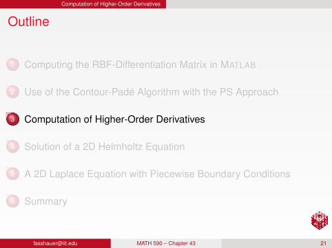
Outline
1 Computing the RBF-Differentiation Matrix in MATLAB
2 Use of the Contour-Padé Algorithm with the PS Approach
3 Computation of Higher-Order Derivatives
4 Solution of a 2D Helmholtz Equation
5 A 2D Laplace Equation with Piecewise Boundary Conditions
6 Summary
[email protected] MATH 590 – Chapter 43 21
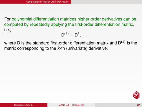
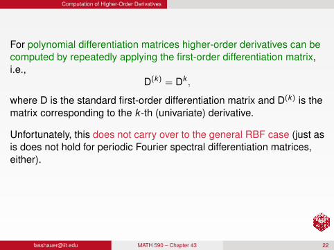
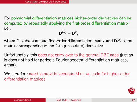
Computation of Higher-Order Derivatives
For polynomial differentiation matrices higher-order derivatives can becomputed by repeatedly applying the first-order differentiation matrix,i.e.,
D(k) = Dk ,
where D is the standard first-order differentiation matrix and D(k) is thematrix corresponding to the k -th (univariate) derivative.
Unfortunately, this does not carry over to the general RBF case (just asis does not hold for periodic Fourier spectral differentiation matrices,either).
We therefore need to provide separate MATLAB code for higher-orderdifferentiation matrices.
[email protected] MATH 590 – Chapter 43 22
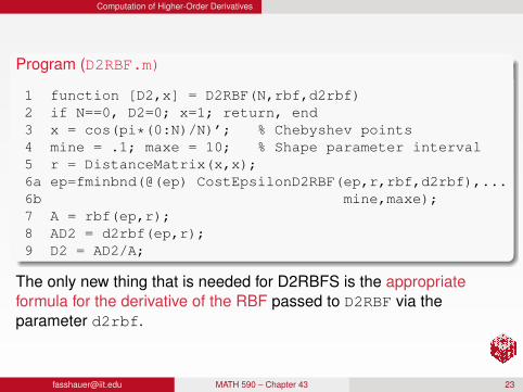
Computation of Higher-Order Derivatives
Program (D2RBF.m)
1 function [D2,x] = D2RBF(N,rbf,d2rbf)2 if N==0, D2=0; x=1; return, end3 x = cos(pi*(0:N)/N)’; % Chebyshev points4 mine = .1; maxe = 10; % Shape parameter interval5 r = DistanceMatrix(x,x);6a ep=fminbnd(@(ep) CostEpsilonD2RBF(ep,r,rbf,d2rbf),...6b mine,maxe);7 A = rbf(ep,r);8 AD2 = d2rbf(ep,r);9 D2 = AD2/A;
The only new thing that is needed for D2RBFS is the appropriateformula for the derivative of the RBF passed to D2RBF via theparameter d2rbf.
[email protected] MATH 590 – Chapter 43 23

Computation of Higher-Order Derivatives
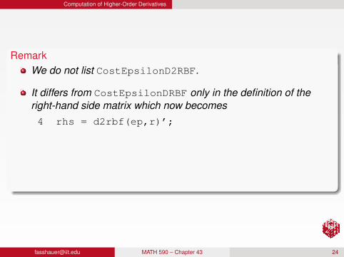
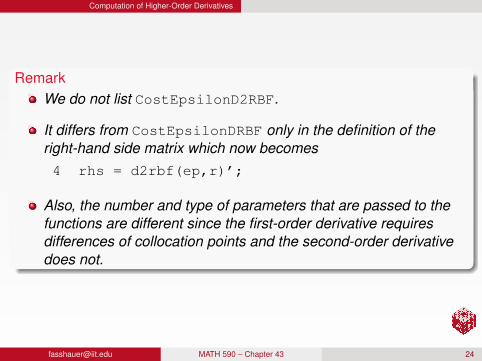
RemarkWe do not list CostEpsilonD2RBF.
It differs from CostEpsilonDRBF only in the definition of theright-hand side matrix which now becomes4 rhs = d2rbf(ep,r)’;
Also, the number and type of parameters that are passed to thefunctions are different since the first-order derivative requiresdifferences of collocation points and the second-order derivativedoes not.
[email protected] MATH 590 – Chapter 43 24
Computation of Higher-Order Derivatives
RemarkWe do not list CostEpsilonD2RBF.
It differs from CostEpsilonDRBF only in the definition of theright-hand side matrix which now becomes4 rhs = d2rbf(ep,r)’;
Also, the number and type of parameters that are passed to thefunctions are different since the first-order derivative requiresdifferences of collocation points and the second-order derivativedoes not.
[email protected] MATH 590 – Chapter 43 24
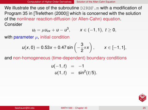
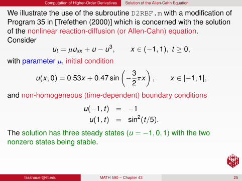
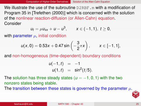
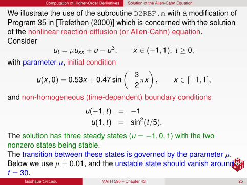
Computation of Higher-Order Derivatives Solution of the Allen-Cahn Equation
We illustrate the use of the subroutine D2RBF.m with a modification ofProgram 35 in [Trefethen (2000)] which is concerned with the solutionof the nonlinear reaction-diffusion (or Allen-Cahn) equation.
Considerut = µuxx + u − u3, x ∈ (−1,1), t ≥ 0,
with parameter µ, initial condition
u(x ,0) = 0.53x + 0.47 sin(−3
2πx), x ∈ [−1,1],
and non-homogeneous (time-dependent) boundary conditions
u(−1, t) = −1u(1, t) = sin2(t/5).
The solution has three steady states (u = −1,0,1) with the twononzero states being stable.The transition between these states is governed by the parameter µ.Below we use µ = 0.01, and the unstable state should vanish aroundt = 30.
[email protected] MATH 590 – Chapter 43 25
Computation of Higher-Order Derivatives Solution of the Allen-Cahn Equation
We illustrate the use of the subroutine D2RBF.m with a modification ofProgram 35 in [Trefethen (2000)] which is concerned with the solutionof the nonlinear reaction-diffusion (or Allen-Cahn) equation.Consider
ut = µuxx + u − u3, x ∈ (−1,1), t ≥ 0,
with parameter µ, initial condition
u(x ,0) = 0.53x + 0.47 sin(−3
2πx), x ∈ [−1,1],
and non-homogeneous (time-dependent) boundary conditions
u(−1, t) = −1u(1, t) = sin2(t/5).
The solution has three steady states (u = −1,0,1) with the twononzero states being stable.
The transition between these states is governed by the parameter µ.Below we use µ = 0.01, and the unstable state should vanish aroundt = 30.
[email protected] MATH 590 – Chapter 43 25
Computation of Higher-Order Derivatives Solution of the Allen-Cahn Equation
We illustrate the use of the subroutine D2RBF.m with a modification ofProgram 35 in [Trefethen (2000)] which is concerned with the solutionof the nonlinear reaction-diffusion (or Allen-Cahn) equation.Consider
ut = µuxx + u − u3, x ∈ (−1,1), t ≥ 0,
with parameter µ, initial condition
u(x ,0) = 0.53x + 0.47 sin(−3
2πx), x ∈ [−1,1],
and non-homogeneous (time-dependent) boundary conditions
u(−1, t) = −1u(1, t) = sin2(t/5).
The solution has three steady states (u = −1,0,1) with the twononzero states being stable.The transition between these states is governed by the parameter µ.
Below we use µ = 0.01, and the unstable state should vanish aroundt = 30.
[email protected] MATH 590 – Chapter 43 25
Computation of Higher-Order Derivatives Solution of the Allen-Cahn Equation
We illustrate the use of the subroutine D2RBF.m with a modification ofProgram 35 in [Trefethen (2000)] which is concerned with the solutionof the nonlinear reaction-diffusion (or Allen-Cahn) equation.Consider
ut = µuxx + u − u3, x ∈ (−1,1), t ≥ 0,
with parameter µ, initial condition
u(x ,0) = 0.53x + 0.47 sin(−3
2πx), x ∈ [−1,1],
and non-homogeneous (time-dependent) boundary conditions
u(−1, t) = −1u(1, t) = sin2(t/5).
The solution has three steady states (u = −1,0,1) with the twononzero states being stable.The transition between these states is governed by the parameter µ.Below we use µ = 0.01, and the unstable state should vanish aroundt = 30.
[email protected] MATH 590 – Chapter 43 25
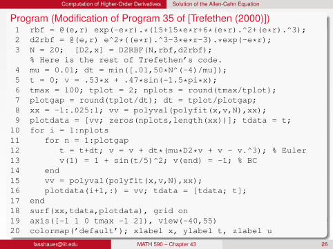
Computation of Higher-Order Derivatives Solution of the Allen-Cahn Equation
Program (Modification of Program 35 of [Trefethen (2000)])1 rbf = @(e,r) exp(-e*r).*(15+15*e*r+6*(e*r).^2+(e*r).^3);2 d2rbf = @(e,r) e^2*((e*r).^3-3*e*r-3).*exp(-e*r);3 N = 20; [D2,x] = D2RBF(N,rbf,d2rbf);
% Here is the rest of Trefethen’s code.4 mu = 0.01; dt = min([.01,50*N^(-4)/mu]);5 t = 0; v = .53*x + .47*sin(-1.5*pi*x);6 tmax = 100; tplot = 2; nplots = round(tmax/tplot);7 plotgap = round(tplot/dt); dt = tplot/plotgap;8 xx = -1:.025:1; vv = polyval(polyfit(x,v,N),xx);9 plotdata = [vv; zeros(nplots,length(xx))]; tdata = t;
10 for i = 1:nplots11 for n = 1:plotgap12 t = t+dt; v = v + dt*(mu*D2*v + v - v.^3); % Euler13 v(1) = 1 + sin(t/5)^2; v(end) = -1; % BC14 end15 vv = polyval(polyfit(x,v,N),xx);16 plotdata(i+1,:) = vv; tdata = [tdata; t];17 end18 surf(xx,tdata,plotdata), grid on19 axis([-1 1 0 tmax -1 2]), view(-40,55)20 colormap(’default’); xlabel x, ylabel t, zlabel u
[email protected] MATH 590 – Chapter 43 26
Computation of Higher-Order Derivatives Solution of the Allen-Cahn Equation
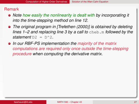
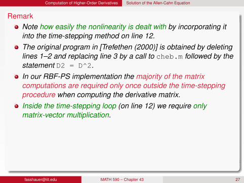
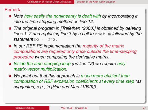
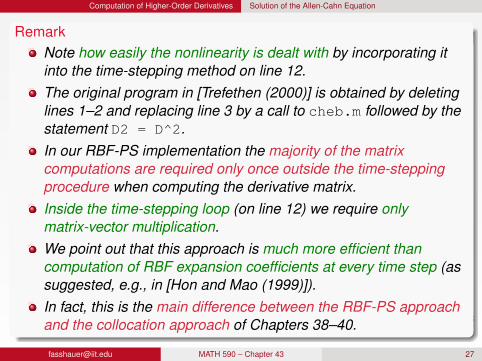
RemarkNote how easily the nonlinearity is dealt with by incorporating itinto the time-stepping method on line 12.
The original program in [Trefethen (2000)] is obtained by deletinglines 1–2 and replacing line 3 by a call to cheb.m followed by thestatement D2 = D^2.In our RBF-PS implementation the majority of the matrixcomputations are required only once outside the time-steppingprocedure when computing the derivative matrix.Inside the time-stepping loop (on line 12) we require onlymatrix-vector multiplication.We point out that this approach is much more efficient thancomputation of RBF expansion coefficients at every time step (assuggested, e.g., in [Hon and Mao (1999)]).In fact, this is the main difference between the RBF-PS approachand the collocation approach of Chapters 38–40.
[email protected] MATH 590 – Chapter 43 27
Computation of Higher-Order Derivatives Solution of the Allen-Cahn Equation
RemarkNote how easily the nonlinearity is dealt with by incorporating itinto the time-stepping method on line 12.The original program in [Trefethen (2000)] is obtained by deletinglines 1–2 and replacing line 3 by a call to cheb.m followed by thestatement D2 = D^2.
In our RBF-PS implementation the majority of the matrixcomputations are required only once outside the time-steppingprocedure when computing the derivative matrix.Inside the time-stepping loop (on line 12) we require onlymatrix-vector multiplication.We point out that this approach is much more efficient thancomputation of RBF expansion coefficients at every time step (assuggested, e.g., in [Hon and Mao (1999)]).In fact, this is the main difference between the RBF-PS approachand the collocation approach of Chapters 38–40.
[email protected] MATH 590 – Chapter 43 27
Computation of Higher-Order Derivatives Solution of the Allen-Cahn Equation
RemarkNote how easily the nonlinearity is dealt with by incorporating itinto the time-stepping method on line 12.The original program in [Trefethen (2000)] is obtained by deletinglines 1–2 and replacing line 3 by a call to cheb.m followed by thestatement D2 = D^2.In our RBF-PS implementation the majority of the matrixcomputations are required only once outside the time-steppingprocedure when computing the derivative matrix.
Inside the time-stepping loop (on line 12) we require onlymatrix-vector multiplication.We point out that this approach is much more efficient thancomputation of RBF expansion coefficients at every time step (assuggested, e.g., in [Hon and Mao (1999)]).In fact, this is the main difference between the RBF-PS approachand the collocation approach of Chapters 38–40.
[email protected] MATH 590 – Chapter 43 27
Computation of Higher-Order Derivatives Solution of the Allen-Cahn Equation
RemarkNote how easily the nonlinearity is dealt with by incorporating itinto the time-stepping method on line 12.The original program in [Trefethen (2000)] is obtained by deletinglines 1–2 and replacing line 3 by a call to cheb.m followed by thestatement D2 = D^2.In our RBF-PS implementation the majority of the matrixcomputations are required only once outside the time-steppingprocedure when computing the derivative matrix.Inside the time-stepping loop (on line 12) we require onlymatrix-vector multiplication.
We point out that this approach is much more efficient thancomputation of RBF expansion coefficients at every time step (assuggested, e.g., in [Hon and Mao (1999)]).In fact, this is the main difference between the RBF-PS approachand the collocation approach of Chapters 38–40.
[email protected] MATH 590 – Chapter 43 27
Computation of Higher-Order Derivatives Solution of the Allen-Cahn Equation
RemarkNote how easily the nonlinearity is dealt with by incorporating itinto the time-stepping method on line 12.The original program in [Trefethen (2000)] is obtained by deletinglines 1–2 and replacing line 3 by a call to cheb.m followed by thestatement D2 = D^2.In our RBF-PS implementation the majority of the matrixcomputations are required only once outside the time-steppingprocedure when computing the derivative matrix.Inside the time-stepping loop (on line 12) we require onlymatrix-vector multiplication.We point out that this approach is much more efficient thancomputation of RBF expansion coefficients at every time step (assuggested, e.g., in [Hon and Mao (1999)]).
In fact, this is the main difference between the RBF-PS approachand the collocation approach of Chapters 38–40.
[email protected] MATH 590 – Chapter 43 27
Computation of Higher-Order Derivatives Solution of the Allen-Cahn Equation
RemarkNote how easily the nonlinearity is dealt with by incorporating itinto the time-stepping method on line 12.The original program in [Trefethen (2000)] is obtained by deletinglines 1–2 and replacing line 3 by a call to cheb.m followed by thestatement D2 = D^2.In our RBF-PS implementation the majority of the matrixcomputations are required only once outside the time-steppingprocedure when computing the derivative matrix.Inside the time-stepping loop (on line 12) we require onlymatrix-vector multiplication.We point out that this approach is much more efficient thancomputation of RBF expansion coefficients at every time step (assuggested, e.g., in [Hon and Mao (1999)]).In fact, this is the main difference between the RBF-PS approachand the collocation approach of Chapters 38–40.
[email protected] MATH 590 – Chapter 43 27
Computation of Higher-Order Derivatives Solution of the Allen-Cahn Equation
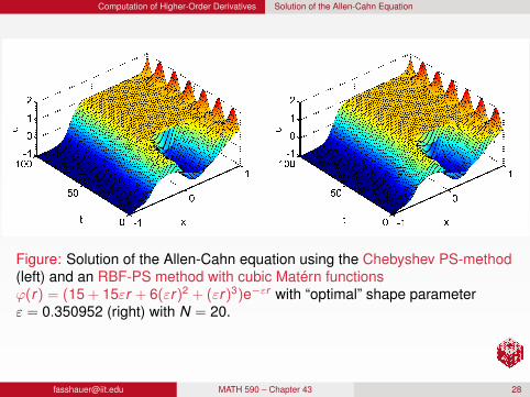
Figure: Solution of the Allen-Cahn equation using the Chebyshev PS-method(left) and an RBF-PS method with cubic Matérn functionsϕ(r) = (15 + 15εr + 6(εr)2 + (εr)3)e−εr with “optimal” shape parameterε = 0.350952 (right) with N = 20.
[email protected] MATH 590 – Chapter 43 28
Computation of Higher-Order Derivatives Solution of the Allen-Cahn Equation
RemarkWe can see that the solution based on Chebyshev polynomialsappears to be slightly more accurate since the transition occurs ata slightly later and correct time (i.e., at t ≈ 30) and is also a little“sharper”.
The differentiation matrix RBF is obtained directly with D2RBF.m(i.e., without the Contour-Padé algorithm – since that method isnot reliable for 21 points).
The plots show that reasonable solutions can also be obtained viathis direct (and much simpler) RBF approach.
True spectral accuracy will no longer be given if ε > 0.
[email protected] MATH 590 – Chapter 43 29
Solution of a 2D Helmholtz Equation
Outline
1 Computing the RBF-Differentiation Matrix in MATLAB
2 Use of the Contour-Padé Algorithm with the PS Approach
3 Computation of Higher-Order Derivatives
4 Solution of a 2D Helmholtz Equation
5 A 2D Laplace Equation with Piecewise Boundary Conditions
6 Summary
[email protected] MATH 590 – Chapter 43 30
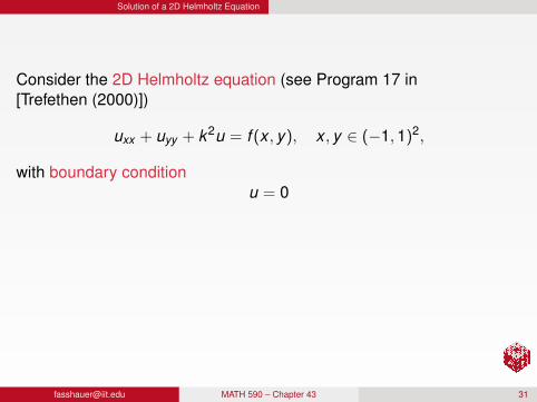
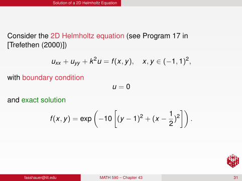
Solution of a 2D Helmholtz Equation
Consider the 2D Helmholtz equation (see Program 17 in[Trefethen (2000)])
uxx + uyy + k2u = f (x , y), x , y ∈ (−1,1)2,
with boundary conditionu = 0
and exact solution
f (x , y) = exp(−10
[(y − 1)2 + (x − 1
2)2])
.
[email protected] MATH 590 – Chapter 43 31
Solution of a 2D Helmholtz Equation
Consider the 2D Helmholtz equation (see Program 17 in[Trefethen (2000)])
uxx + uyy + k2u = f (x , y), x , y ∈ (−1,1)2,
with boundary conditionu = 0
and exact solution
f (x , y) = exp(−10
[(y − 1)2 + (x − 1
2)2])
.
[email protected] MATH 590 – Chapter 43 31
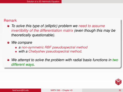
Solution of a 2D Helmholtz Equation
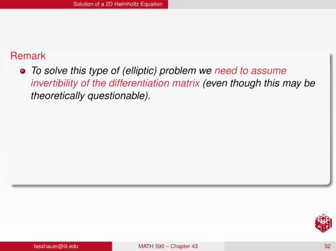
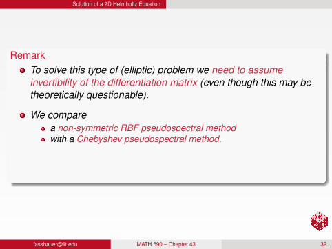
RemarkTo solve this type of (elliptic) problem we need to assumeinvertibility of the differentiation matrix (even though this may betheoretically questionable).
We comparea non-symmetric RBF pseudospectral methodwith a Chebyshev pseudospectral method.
We attempt to solve the problem with radial basis functions in twodifferent ways.
[email protected] MATH 590 – Chapter 43 32
Solution of a 2D Helmholtz Equation
RemarkTo solve this type of (elliptic) problem we need to assumeinvertibility of the differentiation matrix (even though this may betheoretically questionable).
We comparea non-symmetric RBF pseudospectral methodwith a Chebyshev pseudospectral method.
We attempt to solve the problem with radial basis functions in twodifferent ways.
[email protected] MATH 590 – Chapter 43 32
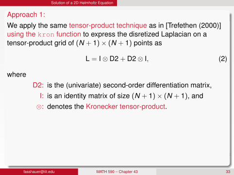
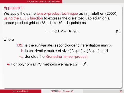
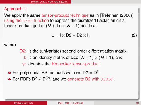
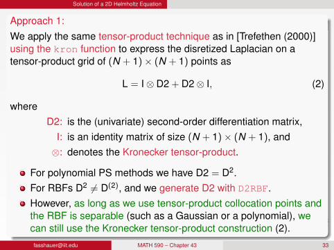
Solution of a 2D Helmholtz Equation
Approach 1:We apply the same tensor-product technique as in [Trefethen (2000)]using the kron function to express the disretized Laplacian on atensor-product grid of (N + 1)× (N + 1) points as
L = I⊗ D2 + D2⊗ I, (2)
whereD2: is the (univariate) second-order differentiation matrix,
I: is an identity matrix of size (N + 1)× (N + 1), and⊗: denotes the Kronecker tensor-product.
For polynomial PS methods we have D2 = D2.For RBFs D2 6= D(2), and we generate D2 with D2RBF.However, as long as we use tensor-product collocation points andthe RBF is separable (such as a Gaussian or a polynomial), wecan still use the Kronecker tensor-product construction (2).
[email protected] MATH 590 – Chapter 43 33
Solution of a 2D Helmholtz Equation
Approach 1:We apply the same tensor-product technique as in [Trefethen (2000)]using the kron function to express the disretized Laplacian on atensor-product grid of (N + 1)× (N + 1) points as
L = I⊗ D2 + D2⊗ I, (2)
whereD2: is the (univariate) second-order differentiation matrix,
I: is an identity matrix of size (N + 1)× (N + 1), and⊗: denotes the Kronecker tensor-product.
For polynomial PS methods we have D2 = D2.
For RBFs D2 6= D(2), and we generate D2 with D2RBF.However, as long as we use tensor-product collocation points andthe RBF is separable (such as a Gaussian or a polynomial), wecan still use the Kronecker tensor-product construction (2).
[email protected] MATH 590 – Chapter 43 33
Solution of a 2D Helmholtz Equation
Approach 1:We apply the same tensor-product technique as in [Trefethen (2000)]using the kron function to express the disretized Laplacian on atensor-product grid of (N + 1)× (N + 1) points as
L = I⊗ D2 + D2⊗ I, (2)
whereD2: is the (univariate) second-order differentiation matrix,
I: is an identity matrix of size (N + 1)× (N + 1), and⊗: denotes the Kronecker tensor-product.
For polynomial PS methods we have D2 = D2.For RBFs D2 6= D(2), and we generate D2 with D2RBF.
However, as long as we use tensor-product collocation points andthe RBF is separable (such as a Gaussian or a polynomial), wecan still use the Kronecker tensor-product construction (2).
[email protected] MATH 590 – Chapter 43 33
Solution of a 2D Helmholtz Equation
Approach 1:We apply the same tensor-product technique as in [Trefethen (2000)]using the kron function to express the disretized Laplacian on atensor-product grid of (N + 1)× (N + 1) points as
L = I⊗ D2 + D2⊗ I, (2)
whereD2: is the (univariate) second-order differentiation matrix,
I: is an identity matrix of size (N + 1)× (N + 1), and⊗: denotes the Kronecker tensor-product.
For polynomial PS methods we have D2 = D2.For RBFs D2 6= D(2), and we generate D2 with D2RBF.However, as long as we use tensor-product collocation points andthe RBF is separable (such as a Gaussian or a polynomial), wecan still use the Kronecker tensor-product construction (2).
[email protected] MATH 590 – Chapter 43 33
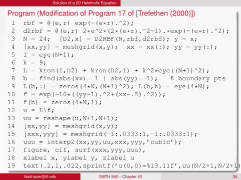
Solution of a 2D Helmholtz Equation
Program (Modification of Program 17 of [Trefethen (2000)])1 rbf = @(e,r) exp(-(e*r).^2);2 d2rbf = @(e,r) 2*e^2*(2*(e*r).^2-1).*exp(-(e*r).^2);3 N = 24; [D2,x] = D2RBF(N,rbf,d2rbf); y = x;4 [xx,yy] = meshgrid(x,y); xx = xx(:); yy = yy(:);5 I = eye(N+1);6 k = 9;7 L = kron(I,D2) + kron(D2,I) + k^2*eye((N+1)^2);8 b = find(abs(xx)==1 | abs(yy)==1); % boundary pts9 L(b,:) = zeros(4*N,(N+1)^2); L(b,b) = eye(4*N);
10 f = exp(-10*((yy-1).^2+(xx-.5).^2));11 f(b) = zeros(4*N,1);12 u = L\f;13 uu = reshape(u,N+1,N+1);14 [xx,yy] = meshgrid(x,y);15 [xxx,yyy] = meshgrid(-1:.0333:1,-1:.0333:1);16 uuu = interp2(xx,yy,uu,xxx,yyy,’cubic’);17 figure, clf, surf(xxx,yyy,uuu),18 xlabel x, ylabel y, zlabel u19 text(.2,1,.022,sprintf(’u(0,0)=%13.11f’,uu(N/2+1,N/2+1)))
[email protected] MATH 590 – Chapter 43 34
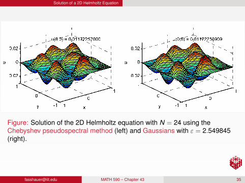
Solution of a 2D Helmholtz Equation
Figure: Solution of the 2D Helmholtz equation with N = 24 using theChebyshev pseudospectral method (left) and Gaussians with ε = 2.549845(right).
[email protected] MATH 590 – Chapter 43 35
Solution of a 2D Helmholtz Equation
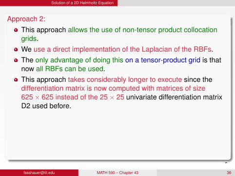
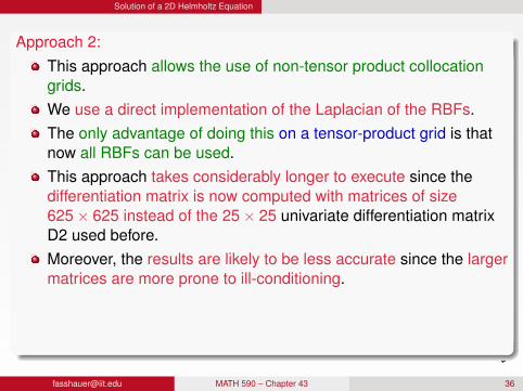
Approach 2:This approach allows the use of non-tensor product collocationgrids.
We use a direct implementation of the Laplacian of the RBFs.The only advantage of doing this on a tensor-product grid is thatnow all RBFs can be used.This approach takes considerably longer to execute since thedifferentiation matrix is now computed with matrices of size625× 625 instead of the 25× 25 univariate differentiation matrixD2 used before.Moreover, the results are likely to be less accurate since the largermatrices are more prone to ill-conditioning.However, the advantage of this approach is that it frees us of thelimitation of polynomial PS methods to tensor-product collocationgrids.
[email protected] MATH 590 – Chapter 43 36
Solution of a 2D Helmholtz Equation
Approach 2:This approach allows the use of non-tensor product collocationgrids.We use a direct implementation of the Laplacian of the RBFs.
The only advantage of doing this on a tensor-product grid is thatnow all RBFs can be used.This approach takes considerably longer to execute since thedifferentiation matrix is now computed with matrices of size625× 625 instead of the 25× 25 univariate differentiation matrixD2 used before.Moreover, the results are likely to be less accurate since the largermatrices are more prone to ill-conditioning.However, the advantage of this approach is that it frees us of thelimitation of polynomial PS methods to tensor-product collocationgrids.
[email protected] MATH 590 – Chapter 43 36
Solution of a 2D Helmholtz Equation
Approach 2:This approach allows the use of non-tensor product collocationgrids.We use a direct implementation of the Laplacian of the RBFs.The only advantage of doing this on a tensor-product grid is thatnow all RBFs can be used.
This approach takes considerably longer to execute since thedifferentiation matrix is now computed with matrices of size625× 625 instead of the 25× 25 univariate differentiation matrixD2 used before.Moreover, the results are likely to be less accurate since the largermatrices are more prone to ill-conditioning.However, the advantage of this approach is that it frees us of thelimitation of polynomial PS methods to tensor-product collocationgrids.
[email protected] MATH 590 – Chapter 43 36
Solution of a 2D Helmholtz Equation
Approach 2:This approach allows the use of non-tensor product collocationgrids.We use a direct implementation of the Laplacian of the RBFs.The only advantage of doing this on a tensor-product grid is thatnow all RBFs can be used.This approach takes considerably longer to execute since thedifferentiation matrix is now computed with matrices of size625× 625 instead of the 25× 25 univariate differentiation matrixD2 used before.
Moreover, the results are likely to be less accurate since the largermatrices are more prone to ill-conditioning.However, the advantage of this approach is that it frees us of thelimitation of polynomial PS methods to tensor-product collocationgrids.
[email protected] MATH 590 – Chapter 43 36
Solution of a 2D Helmholtz Equation
Approach 2:This approach allows the use of non-tensor product collocationgrids.We use a direct implementation of the Laplacian of the RBFs.The only advantage of doing this on a tensor-product grid is thatnow all RBFs can be used.This approach takes considerably longer to execute since thedifferentiation matrix is now computed with matrices of size625× 625 instead of the 25× 25 univariate differentiation matrixD2 used before.Moreover, the results are likely to be less accurate since the largermatrices are more prone to ill-conditioning.
However, the advantage of this approach is that it frees us of thelimitation of polynomial PS methods to tensor-product collocationgrids.
[email protected] MATH 590 – Chapter 43 36
Solution of a 2D Helmholtz Equation
Approach 2:This approach allows the use of non-tensor product collocationgrids.We use a direct implementation of the Laplacian of the RBFs.The only advantage of doing this on a tensor-product grid is thatnow all RBFs can be used.This approach takes considerably longer to execute since thedifferentiation matrix is now computed with matrices of size625× 625 instead of the 25× 25 univariate differentiation matrixD2 used before.Moreover, the results are likely to be less accurate since the largermatrices are more prone to ill-conditioning.However, the advantage of this approach is that it frees us of thelimitation of polynomial PS methods to tensor-product collocationgrids.
[email protected] MATH 590 – Chapter 43 36
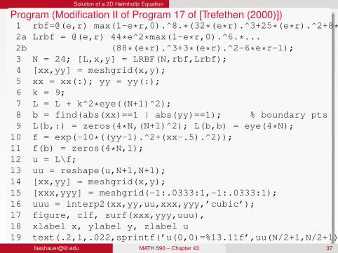
Solution of a 2D Helmholtz Equation
Program (Modification II of Program 17 of [Trefethen (2000)])1 rbf=@(e,r) max(1-e*r,0).^8.*(32*(e*r).^3+25*(e*r).^2+8*e*r+1);2a Lrbf = @(e,r) 44*e^2*max(1-e*r,0).^6.*...2b (88*(e*r).^3+3*(e*r).^2-6*e*r-1);3 N = 24; [L,x,y] = LRBF(N,rbf,Lrbf);4 [xx,yy] = meshgrid(x,y);5 xx = xx(:); yy = yy(:);6 k = 9;7 L = L + k^2*eye((N+1)^2);8 b = find(abs(xx)==1 | abs(yy)==1); % boundary pts9 L(b,:) = zeros(4*N,(N+1)^2); L(b,b) = eye(4*N);
10 f = exp(-10*((yy-1).^2+(xx-.5).^2));11 f(b) = zeros(4*N,1);12 u = L\f;13 uu = reshape(u,N+1,N+1);14 [xx,yy] = meshgrid(x,y);15 [xxx,yyy] = meshgrid(-1:.0333:1,-1:.0333:1);16 uuu = interp2(xx,yy,uu,xxx,yyy,’cubic’);17 figure, clf, surf(xxx,yyy,uuu),18 xlabel x, ylabel y, zlabel u19 text(.2,1,.022,sprintf(’u(0,0)=%13.11f’,uu(N/2+1,N/2+1)))
[email protected] MATH 590 – Chapter 43 37
Solution of a 2D Helmholtz Equation
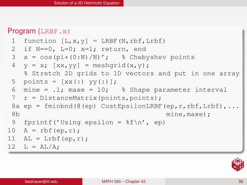
Program (LRBF.m)1 function [L,x,y] = LRBF(N,rbf,Lrbf)2 if N==0, L=0; x=1; return, end3 x = cos(pi*(0:N)/N)’; % Chebyshev points4 y = x; [xx,yy] = meshgrid(x,y);
% Stretch 2D grids to 1D vectors and put in one array5 points = [xx(:) yy(:)];6 mine = .1; maxe = 10; % Shape parameter interval7 r = DistanceMatrix(points,points);8a ep = fminbnd(@(ep) CostEpsilonLRBF(ep,r,rbf,Lrbf),...8b mine,maxe);9 fprintf(’Using epsilon = %f\n’, ep)
10 A = rbf(ep,r);11 AL = Lrbf(ep,r);12 L = AL/A;
[email protected] MATH 590 – Chapter 43 38
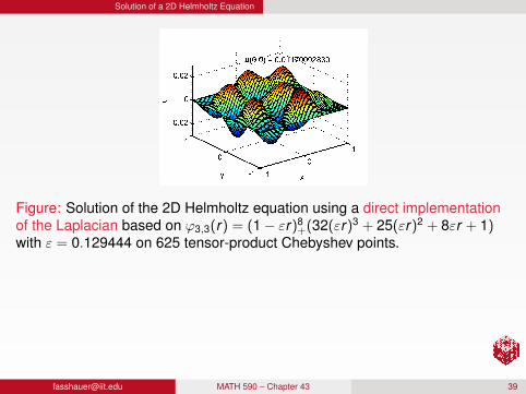
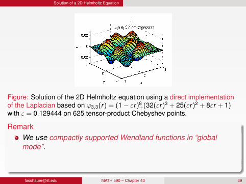
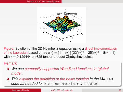
Solution of a 2D Helmholtz Equation
Figure: Solution of the 2D Helmholtz equation using a direct implementationof the Laplacian based on ϕ3,3(r) = (1− εr)8
+(32(εr)3 + 25(εr)2 + 8εr + 1)with ε = 0.129444 on 625 tensor-product Chebyshev points.
RemarkWe use compactly supported Wendland functions in “globalmode”.This explains the definition of the basic function in the MATLAB
code as needed for DistanceMatrix.m in LRBF.m.
[email protected] MATH 590 – Chapter 43 39
Solution of a 2D Helmholtz Equation
Figure: Solution of the 2D Helmholtz equation using a direct implementationof the Laplacian based on ϕ3,3(r) = (1− εr)8
+(32(εr)3 + 25(εr)2 + 8εr + 1)with ε = 0.129444 on 625 tensor-product Chebyshev points.
RemarkWe use compactly supported Wendland functions in “globalmode”.
This explains the definition of the basic function in the MATLAB
code as needed for DistanceMatrix.m in LRBF.m.
[email protected] MATH 590 – Chapter 43 39
Solution of a 2D Helmholtz Equation
Figure: Solution of the 2D Helmholtz equation using a direct implementationof the Laplacian based on ϕ3,3(r) = (1− εr)8
+(32(εr)3 + 25(εr)2 + 8εr + 1)with ε = 0.129444 on 625 tensor-product Chebyshev points.
RemarkWe use compactly supported Wendland functions in “globalmode”.This explains the definition of the basic function in the MATLAB
code as needed for DistanceMatrix.m in LRBF.m.
[email protected] MATH 590 – Chapter 43 39
A 2D Laplace Equation with Piecewise Boundary Conditions
Outline
1 Computing the RBF-Differentiation Matrix in MATLAB
2 Use of the Contour-Padé Algorithm with the PS Approach
3 Computation of Higher-Order Derivatives
4 Solution of a 2D Helmholtz Equation
5 A 2D Laplace Equation with Piecewise Boundary Conditions
6 Summary
[email protected] MATH 590 – Chapter 43 40
A 2D Laplace Equation with Piecewise Boundary Conditions
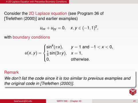
Consider the 2D Laplace equation (see Program 36 of[Trefethen (2000)] and earlier examples)
uxx + uyy = 0, x , y ∈ (−1,1)2,
with boundary conditions
u(x , y) =
sin4(πx), y = 1 and −1 < x < 0,15 sin(3πy), x = 1,0, otherwise.
RemarkWe don’t list the code since it is too similar to previous examples andthe original code in [Trefethen (2000)].
[email protected] MATH 590 – Chapter 43 41
A 2D Laplace Equation with Piecewise Boundary Conditions
−1−0.5
00.5
1
−1
0
1
0
0.5
1
x
u(0,0) = 0.0495946503
y
u
−1−0.5
00.5
1
−1
0
1
0
0.5
1
x
u(0,0) = 0.0495940466
y
u
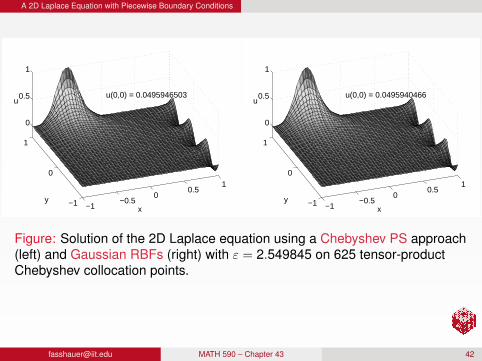
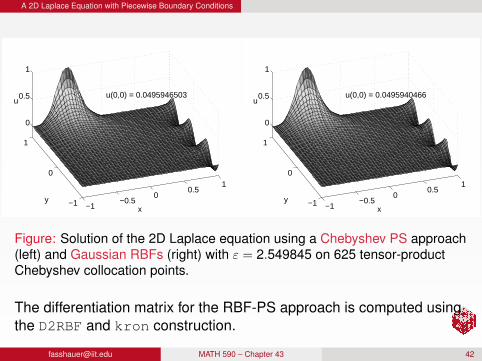
Figure: Solution of the 2D Laplace equation using a Chebyshev PS approach(left) and Gaussian RBFs (right) with ε = 2.549845 on 625 tensor-productChebyshev collocation points.
The differentiation matrix for the RBF-PS approach is computed usingthe D2RBF and kron construction.
[email protected] MATH 590 – Chapter 43 42
A 2D Laplace Equation with Piecewise Boundary Conditions
−1−0.5
00.5
1
−1
0
1
0
0.5
1
x
u(0,0) = 0.0495946503
y
u
−1−0.5
00.5
1
−1
0
1
0
0.5
1
x
u(0,0) = 0.0495940466
y
u
Figure: Solution of the 2D Laplace equation using a Chebyshev PS approach(left) and Gaussian RBFs (right) with ε = 2.549845 on 625 tensor-productChebyshev collocation points.
The differentiation matrix for the RBF-PS approach is computed usingthe D2RBF and kron construction.
[email protected] MATH 590 – Chapter 43 42
Summary
Outline
1 Computing the RBF-Differentiation Matrix in MATLAB
2 Use of the Contour-Padé Algorithm with the PS Approach
3 Computation of Higher-Order Derivatives
4 Solution of a 2D Helmholtz Equation
5 A 2D Laplace Equation with Piecewise Boundary Conditions
6 Summary
[email protected] MATH 590 – Chapter 43 43
Summary
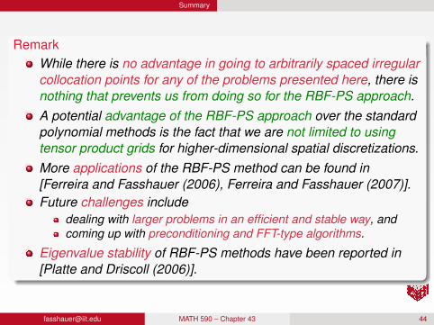
RemarkWhile there is no advantage in going to arbitrarily spaced irregularcollocation points for any of the problems presented here, there isnothing that prevents us from doing so for the RBF-PS approach.
A potential advantage of the RBF-PS approach over the standardpolynomial methods is the fact that we are not limited to usingtensor product grids for higher-dimensional spatial discretizations.More applications of the RBF-PS method can be found in[Ferreira and Fasshauer (2006), Ferreira and Fasshauer (2007)].Future challenges include
dealing with larger problems in an efficient and stable way, andcoming up with preconditioning and FFT-type algorithms.
Eigenvalue stability of RBF-PS methods have been reported in[Platte and Driscoll (2006)].
[email protected] MATH 590 – Chapter 43 44
Summary
RemarkWhile there is no advantage in going to arbitrarily spaced irregularcollocation points for any of the problems presented here, there isnothing that prevents us from doing so for the RBF-PS approach.A potential advantage of the RBF-PS approach over the standardpolynomial methods is the fact that we are not limited to usingtensor product grids for higher-dimensional spatial discretizations.
More applications of the RBF-PS method can be found in[Ferreira and Fasshauer (2006), Ferreira and Fasshauer (2007)].Future challenges include
dealing with larger problems in an efficient and stable way, andcoming up with preconditioning and FFT-type algorithms.
Eigenvalue stability of RBF-PS methods have been reported in[Platte and Driscoll (2006)].
[email protected] MATH 590 – Chapter 43 44
Summary
RemarkWhile there is no advantage in going to arbitrarily spaced irregularcollocation points for any of the problems presented here, there isnothing that prevents us from doing so for the RBF-PS approach.A potential advantage of the RBF-PS approach over the standardpolynomial methods is the fact that we are not limited to usingtensor product grids for higher-dimensional spatial discretizations.More applications of the RBF-PS method can be found in[Ferreira and Fasshauer (2006), Ferreira and Fasshauer (2007)].
Future challenges includedealing with larger problems in an efficient and stable way, andcoming up with preconditioning and FFT-type algorithms.
Eigenvalue stability of RBF-PS methods have been reported in[Platte and Driscoll (2006)].
[email protected] MATH 590 – Chapter 43 44
Summary
RemarkWhile there is no advantage in going to arbitrarily spaced irregularcollocation points for any of the problems presented here, there isnothing that prevents us from doing so for the RBF-PS approach.A potential advantage of the RBF-PS approach over the standardpolynomial methods is the fact that we are not limited to usingtensor product grids for higher-dimensional spatial discretizations.More applications of the RBF-PS method can be found in[Ferreira and Fasshauer (2006), Ferreira and Fasshauer (2007)].Future challenges include
dealing with larger problems in an efficient and stable way, andcoming up with preconditioning and FFT-type algorithms.
Eigenvalue stability of RBF-PS methods have been reported in[Platte and Driscoll (2006)].
[email protected] MATH 590 – Chapter 43 44
Summary
RemarkWhile there is no advantage in going to arbitrarily spaced irregularcollocation points for any of the problems presented here, there isnothing that prevents us from doing so for the RBF-PS approach.A potential advantage of the RBF-PS approach over the standardpolynomial methods is the fact that we are not limited to usingtensor product grids for higher-dimensional spatial discretizations.More applications of the RBF-PS method can be found in[Ferreira and Fasshauer (2006), Ferreira and Fasshauer (2007)].Future challenges include
dealing with larger problems in an efficient and stable way, andcoming up with preconditioning and FFT-type algorithms.
Eigenvalue stability of RBF-PS methods have been reported in[Platte and Driscoll (2006)].
[email protected] MATH 590 – Chapter 43 44
Appendix References
References I
Buhmann, M. D. (2003).Radial Basis Functions: Theory and Implementations.Cambridge University Press.
Fasshauer, G. E. (2007).Meshfree Approximation Methods with MATLAB.World Scientific Publishers.
Higham, D. J. and Higham, N. J. (2005).MATLAB Guide.SIAM (2nd ed.), Philadelphia.
Iske, A. (2004).Multiresolution Methods in Scattered Data Modelling.Lecture Notes in Computational Science and Engineering 37, Springer Verlag(Berlin).
Trefethen, L. N. (2000).Spectral Methods in MATLAB.SIAM (Philadelphia, PA).
[email protected] MATH 590 – Chapter 43 45
Appendix References
References II
G. Wahba (1990).Spline Models for Observational Data.CBMS-NSF Regional Conference Series in Applied Mathematics 59, SIAM(Philadelphia).
Wendland, H. (2005a).Scattered Data Approximation.Cambridge University Press (Cambridge).
Ferreira, A. J. M. and Fasshauer, G. E. (2006)Computation of natural frequencies of shear deformable beams and plates by anRBF-pseudospectral method.Comput. Meth. Appl. Mech. Engng. 196, 134–146.
Ferreira, A. J. M. and Fasshauer, G. E. (2007)Analysis of natural frequencies of composite plates by an RBF-pseudospectralmethod.Composite Structures 79, pp. 202–210.
[email protected] MATH 590 – Chapter 43 46

Appendix References
References III
Fornberg, B. and Wright, G. (2004).Stable computation of multiquadric interpolants for all values of the shapeparameter.Comput. Math. Appl. 47, pp. 497–523.
Hon, Y. C. and Mao, X. Z. (1999).A radial basis function method for solving options pricing model.Financial Engineering 8, pp. 31–49.
Platte, R. B. and Driscoll, T. A. (2006).Eigenvalue stability of radial basis function discretizations for time-dependentproblems.Comput. Math. Appl. 51 8, pp. 1251–1268.
Rippa, S. (1999).An algorithm for selecting a good value for the parameter c in radial basisfunction interpolation.Adv. in Comput. Math. 11, pp. 193–210.
[email protected] MATH 590 – Chapter 43 47


![MATH 590: Meshfree Methodsfass/590/notes/Notes590_Ch9.pdfMATH 590: Meshfree Methods “Flat” Limits of Kernel Interpolants ... LYY07, Sch05, Sch08]). For example,if the data sites](https://img.pdfslide.net/doc/110x75/5a9e64e67f8b9a8e178b48e9/pdfmath-590-meshfree-fass590notesnotes590ch9pdfmath-590-meshfree-methods.jpg)


![Galerking Weak Form [G.R. Liu] Meshfree Methods Moving Beyond the Fin(BookZZ.org)](https://img.pdfslide.net/doc/110x75/55cf8f5f550346703b9bb319/galerking-weak-form-gr-liu-meshfree-methods-moving-beyond-the-finbookzzorg.jpg)