DRAFT V2.1

From

Math, Numerics, & Programming

(for Mechanical Engineers)

Masayuki Yano

James Douglass Penn

George Konidaris

Anthony T Patera

August 2013

© The Authors. License: Creative Commons Attribution-Noncommercial-Share Alike 3.0 (CC BY-NC-SA 3.0), which permits unrestricted use,distribution, and reproduction in any medium, provided the original authors and MIT OpenCourseWare source are credited; the use isnon-commercial; and the CC BY-NC-SA license is retained. See also http://ocw.mit.edu/terms/.

©MIT 2011, 2012, 2013

Unit I

(Numerical) Calculus. ElementaryProgramming Concepts.

11

Chapter 1

Motivation

1.1 A Mobile Robot

Robot self-localization, or the ability of a robot to figure out where it is within its environment, isarguably the most fundamental skill for a mobile robot, such as the one shown in Figure 1.1. Wecan divide the robot self-localization problem into two parts: global position estimation and localposition tracking. Global position estimation is the robot’s ability to determine its initial positionand orientation (collectively, pose) within a known map of its environment. Local position trackingis then the ability of the robot to track changes in its pose over time. In this assignment, we willconsider two basic approaches to global position estimation and local position tracking.

1.2 Global Position Estimation: Infra-red Range-Finding

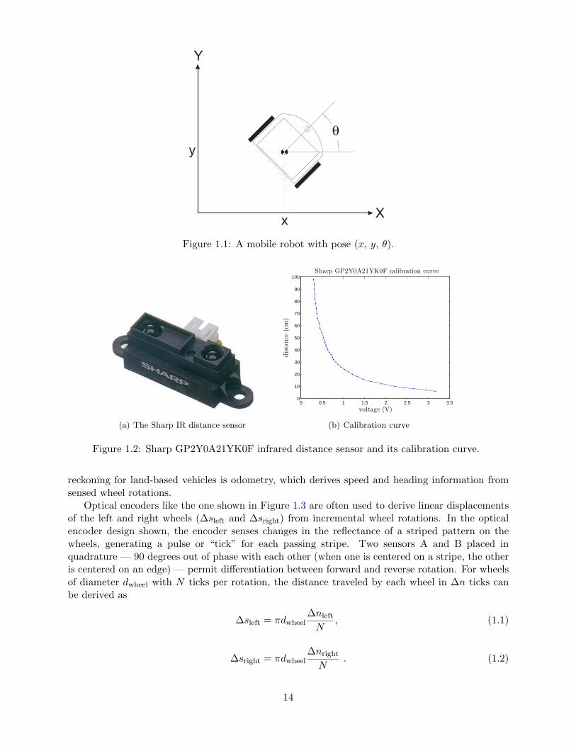
Many systems exist today for robot global position estimation. Perhaps the most familiar exampleis the Global Positioning System (GPS), a network of 24 satellites that can give an absolute po-sition estimate accurate to within several meters. For smaller scale position estimation, high-endsolutions such as robotic vision and laser range-finding can provide millimeter accuracy distancemeasurements, which can then be matched with map data to convert local distance measurementsto global position. As an alternative to these more expensive systems, ultrasonic and infrared dis-tance sensors can offer similar performance with modest compromises in speed and accuracy. Ofthese two, infrared distance sensors often have slightly narrower beam width and faster response.

Figure 1.2(a) shows the Sharp GP2Y0A21YK0F, a popular medium range (10-80 cm), infrared(IR) distance sensor. The Sharp sensor uses triangulation to calculate distance by measuring theangle of incidence of a transmitted IR beam reflected from a distant surface onto a receiving posi-tion sensitive device (PSD). Because the angle is a nonlinear function of the distance to the surface,the Sharp sensor has the nonlinear calibration curve shown in Figure 1.2(b). Given discrete cali-bration data, we can linearly interpolate voltage readings taken from the sensor to derive distancemeasurements.

1.3 Local Position Tracking: Odometry

Dead reckoning, which tracks location by integrating a moving system’s speed and heading overtime, forms the backbone of many mobile robot navigation systems. The simplest form of dead

13

DRAFT V2.1 © The Authors. License: Creative Commons BY-NC-SA 3.0.

X

Y

x

y

q

Figure 1.1: A mobile robot with pose (x, y, θ).

(a) The Sharp IR distance sensor

0 0.5 1 1.5 2 2.5 3 3.50

10

20

30

40

50

60

70

80

90

100

voltage (V)

distance

(cm)

Sharp GP2Y0A21YK0F calibration curve

(b) Calibration curve

Figure 1.2: Sharp GP2Y0A21YK0F infrared distance sensor and its calibration curve.

reckoning for land-based vehicles is odometry, which derives speed and heading information fromsensed wheel rotations.

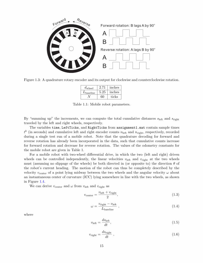
Optical encoders like the one shown in Figure 1.3 are often used to derive linear displacementsof the left and right wheels (∆sleft and ∆sright) from incremental wheel rotations. In the opticalencoder design shown, the encoder senses changes in the reflectance of a striped pattern on thewheels, generating a pulse or “tick” for each passing stripe. Two sensors A and B placed inquadrature — 90 degrees out of phase with each other (when one is centered on a stripe, the otheris centered on an edge) — permit differentiation between forward and reverse rotation. For wheelsof diameter dwheel with N ticks per rotation, the distance traveled by each wheel in ∆n ticks canbe derived as

∆sleft = πdwheel∆nleft

N, (1.1)

∆sright = πdwheel∆nright

N. (1.2)

14

A B

Forward Reverse

A

B

Forward rotation: B lags A by 90o

A

B

Reverse rotation: A lags B by 90o

Figure 1.3: A quadrature rotary encoder and its output for clockwise and counterclockwise rotation.

dwheel 2.71 inches

Lbaseline 5.25 inches

N 60 ticks

Table 1.1: Mobile robot parameters.

By “summing up” the increments, we can compute the total cumulative distances sleft and sright

traveled by the left and right wheels, respectively.The variables time, LeftTicks, and RightTicks from assignment1.mat contain sample times

tk (in seconds) and cumulative left and right encoder counts nleft and nright, respectively, recordedduring a single test run of a mobile robot. Note that the quadrature decoding for forward andreverse rotation has already been incorporated in the data, such that cumulative counts increasefor forward rotation and decrease for reverse rotation. The values of the odometry constants forthe mobile robot are given in Table 1.

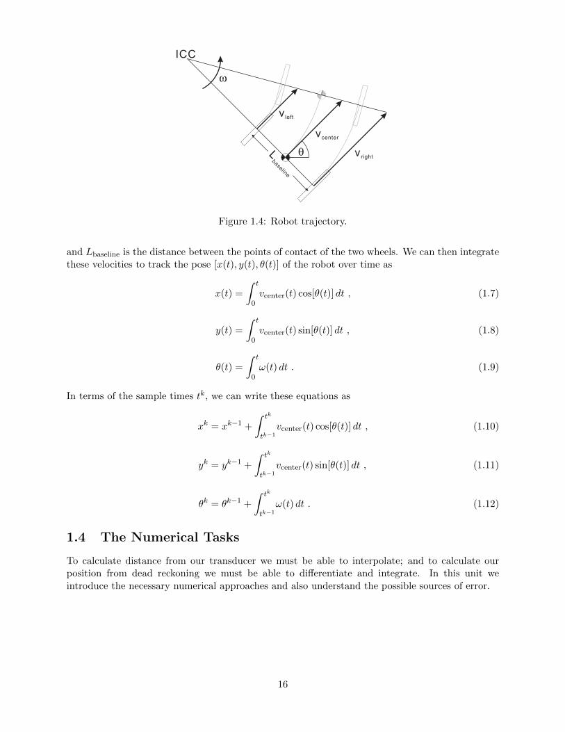
For a mobile robot with two-wheel differential drive, in which the two (left and right) drivenwheels can be controlled independently, the linear velocities vleft and vright at the two wheelsmust (assuming no slippage of the wheels) be both directed in (or opposite to) the direction θ ofthe robot’s current heading. The motion of the robot can thus be completely described by thevelocity vcenter of a point lying midway between the two wheels and the angular velocity ω aboutan instantaneous center of curvature (ICC) lying somewhere in line with the two wheels, as shownin Figure 1.4.

We can derive vcenter and ω from vleft and vright as

vcenter =vleft + vright

2, (1.3)

ω =vright − vleft

Lbaseline, (1.4)

where

vleft =dsleft

dt, (1.5)

vright =dsright

dt, (1.6)

15

qLbaseline

ICC

v right

vcenter

v left

w

Figure 1.4: Robot trajectory.

and Lbaseline is the distance between the points of contact of the two wheels. We can then integratethese velocities to track the pose [x(t), y(t), θ(t)] of the robot over time as

x(t) =

∫ t

0vcenter(t) cos[θ(t)] dt , (1.7)

y(t) =

∫ t

0vcenter(t) sin[θ(t)] dt , (1.8)

θ(t) =

∫ t

0ω(t) dt . (1.9)

In terms of the sample times tk, we can write these equations as

xk = xk−1 +

∫ tk

tk−1

vcenter(t) cos[θ(t)] dt , (1.10)

yk = yk−1 +

∫ tk

tk−1

vcenter(t) sin[θ(t)] dt , (1.11)

θk = θk−1 +

∫ tk

tk−1

ω(t) dt . (1.12)

1.4 The Numerical Tasks

To calculate distance from our transducer we must be able to interpolate; and to calculate ourposition from dead reckoning we must be able to differentiate and integrate. In this unit weintroduce the necessary numerical approaches and also understand the possible sources of error.

16

Chapter 2

Interpolation

2.1 Interpolation of Univariate Functions

The objective of interpolation is to approximate the behavior of a true underlying function usingfunction values at a limited number of points. Interpolation serves two important, distinct purposesthroughout this book. First, it is a mathematical tool that facilitates development and analysisof numerical techniques for, for example, integrating functions and solving differential equations.Second, interpolation can be used to estimate or infer the function behavior based on the functionvalues recorded as a table, for example collected in an experiment (i.e., table lookup).

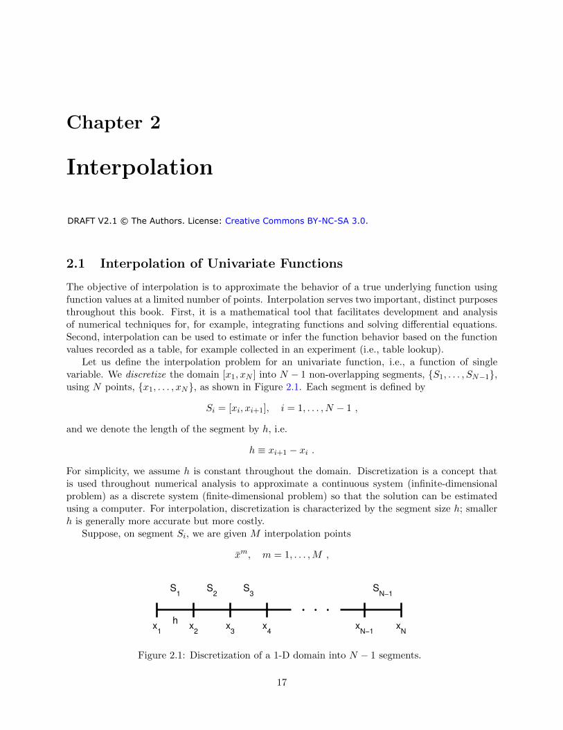
Let us define the interpolation problem for an univariate function, i.e., a function of singlevariable. We discretize the domain [x1, xN ] into N − 1 non-overlapping segments, {S1, . . . , SN−1},using N points, {x1, . . . , xN}, as shown in Figure 2.1. Each segment is defined by

Si = [xi, xi+1], i = 1, . . . , N − 1 ,

and we denote the length of the segment by h, i.e.

h ≡ xi+1 − xi .

For simplicity, we assume h is constant throughout the domain. Discretization is a concept thatis used throughout numerical analysis to approximate a continuous system (infinite-dimensionalproblem) as a discrete system (finite-dimensional problem) so that the solution can be estimatedusing a computer. For interpolation, discretization is characterized by the segment size h; smallerh is generally more accurate but more costly.

Suppose, on segment Si, we are given M interpolation points

xm, m = 1, . . . ,M ,

x1

x2

x3

x4

S1

S2

S3

hx

N−1x

N

SN−1

Figure 2.1: Discretization of a 1-D domain into N − 1 segments.

17

DRAFT V2.1 © The Authors. License: Creative Commons BY-NC-SA 3.0.

x1

x2

x3

x4

x5

S2

discretization

x1 x2 x3

local segment S2

x1

x2

x3

x4

x5

x6

x7

x8

x9

function evaluation points

(a) discretization

ei

S i

(x1 , f(x1))

(x2 , f(x2))

(x3 , f(x3))

xi xi+1

interpolant

interpolation points

function

(b) local interpolation

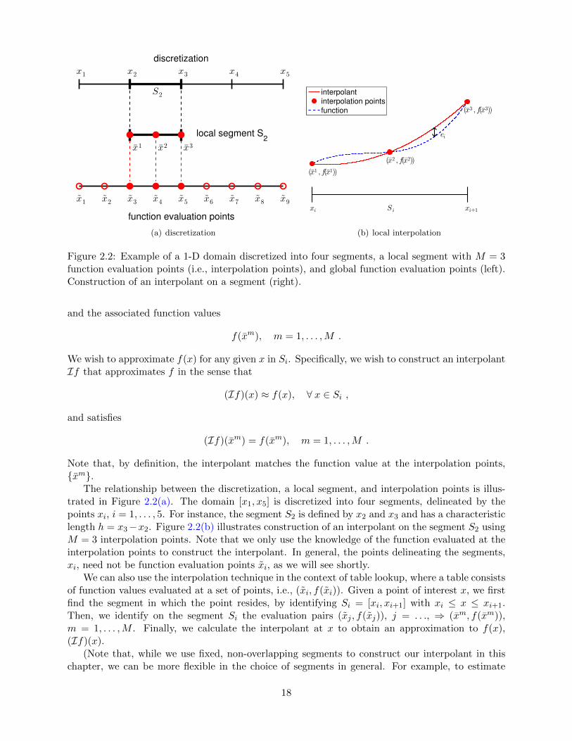
Figure 2.2: Example of a 1-D domain discretized into four segments, a local segment with M = 3function evaluation points (i.e., interpolation points), and global function evaluation points (left).Construction of an interpolant on a segment (right).

and the associated function values

f(xm), m = 1, . . . ,M .

We wish to approximate f(x) for any given x in Si. Specifically, we wish to construct an interpolantIf that approximates f in the sense that

(If)(x) ≈ f(x), ∀ x ∈ Si ,

and satisfies

(If)(xm) = f(xm), m = 1, . . . ,M .

Note that, by definition, the interpolant matches the function value at the interpolation points,{xm}.

The relationship between the discretization, a local segment, and interpolation points is illus-trated in Figure 2.2(a). The domain [x1, x5] is discretized into four segments, delineated by thepoints xi, i = 1, . . . , 5. For instance, the segment S2 is defined by x2 and x3 and has a characteristiclength h = x3−x2. Figure 2.2(b) illustrates construction of an interpolant on the segment S2 usingM = 3 interpolation points. Note that we only use the knowledge of the function evaluated at theinterpolation points to construct the interpolant. In general, the points delineating the segments,xi, need not be function evaluation points xi, as we will see shortly.

We can also use the interpolation technique in the context of table lookup, where a table consistsof function values evaluated at a set of points, i.e., (xi, f(xi)). Given a point of interest x, we firstfind the segment in which the point resides, by identifying Si = [xi, xi+1] with xi ≤ x ≤ xi+1.Then, we identify on the segment Si the evaluation pairs (xj , f(xj)), j = . . ., ⇒ (xm, f(xm)),m = 1, . . . ,M . Finally, we calculate the interpolant at x to obtain an approximation to f(x),(If)(x).

(Note that, while we use fixed, non-overlapping segments to construct our interpolant in thischapter, we can be more flexible in the choice of segments in general. For example, to estimate

18

the value of a function at some point x, we can choose a set of M data points in the neighborhoodof x. Using the M points, we construct a local interpolant as in Figure 2.2(b) and infer f(x)by evaluating the interpolant at x. Note that the local interpolant constructed in this mannerimplicitly defines a local segment. The segment “slides” with the target x, i.e., it is adaptivelychosen. In the current chapter on interpolation and in Chapter 7 on integration, we will emphasizethe fixed segment perspective; however, in discussing differentiation in Chapter 3, we will adoptthe sliding segment perspective.)

To assess the quality of the interpolant, we define its error as the maximum difference betweenthe true function and the interpolant in the segment, i.e.

ei ≡ maxx∈Si|f(x)− (If)(x)| .

Because the construction of an interpolant on a given segment is independent of that on anothersegment1, we can analyze the local interpolation error one segment at a time. The locality ofinterpolation construction and error greatly simplifies the error analysis. In addition, we definethe maximum interpolation error, emax, as the maximum error over the entire domain, which isequivalent to the largest of the segment errors, i.e.

emax ≡ maxi=1,...,N−1

ei .

The interpolation error is a measure we use to assess the quality of different interpolation schemes.Specifically, for each interpolation scheme, we bound the error in terms of the function f and thediscretization parameter h to understand how the error changes as the discretization is refined.

Let us consider an example of interpolant.

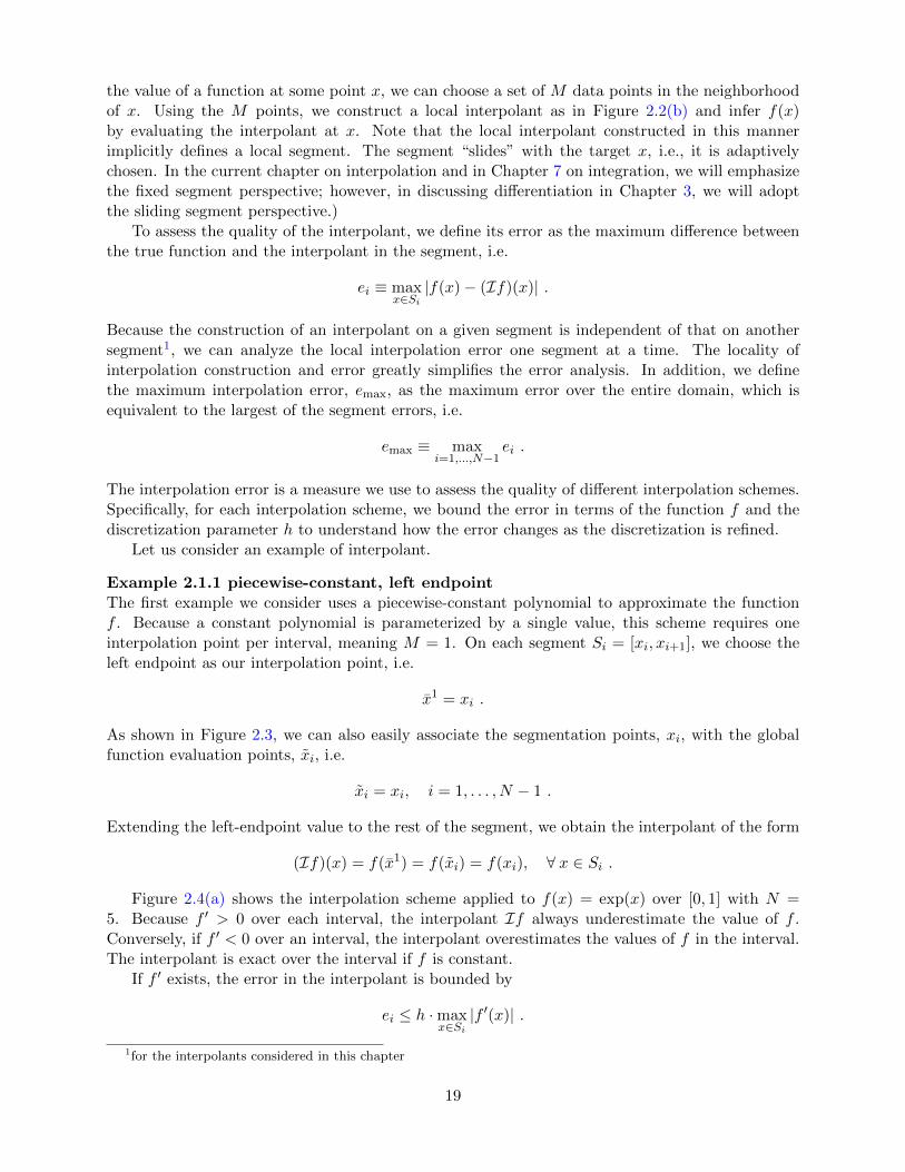
Example 2.1.1 piecewise-constant, left endpointThe first example we consider uses a piecewise-constant polynomial to approximate the functionf . Because a constant polynomial is parameterized by a single value, this scheme requires oneinterpolation point per interval, meaning M = 1. On each segment Si = [xi, xi+1], we choose theleft endpoint as our interpolation point, i.e.

x1 = xi .

As shown in Figure 2.3, we can also easily associate the segmentation points, xi, with the globalfunction evaluation points, xi, i.e.

xi = xi, i = 1, . . . , N − 1 .

Extending the left-endpoint value to the rest of the segment, we obtain the interpolant of the form

(If)(x) = f(x1) = f(xi) = f(xi), ∀ x ∈ Si .

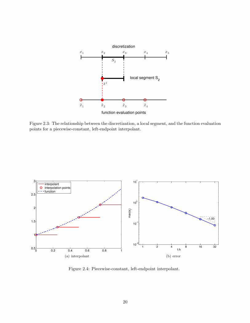
Figure 2.4(a) shows the interpolation scheme applied to f(x) = exp(x) over [0, 1] with N =5. Because f ′ > 0 over each interval, the interpolant If always underestimate the value of f .Conversely, if f ′ < 0 over an interval, the interpolant overestimates the values of f in the interval.The interpolant is exact over the interval if f is constant.

If f ′ exists, the error in the interpolant is bounded by

ei ≤ h ·maxx∈Si|f ′(x)| .

1for the interpolants considered in this chapter

19

x1

x2

x3

x4

x5

S2

discretization

x1

local segment S2

x1

x2

x3

x4

function evaluation points

Figure 2.3: The relationship between the discretization, a local segment, and the function evaluationpoints for a piecewise-constant, left-endpoint interpolant.

0 0.2 0.4 0.6 0.8 10.5

1

1.5

2

2.5

3

interpolant

interpolation points

function

(a) interpolant

1 2 4 8 16 3210

−2

10−1

100

101

−1.00

1/h

ma

x(e

i)

(b) error

Figure 2.4: Piecewise-constant, left-endpoint interpolant.

20

Since ei = O(h) and the error scales as the first power of h, the scheme is said to be first-orderaccurate. The convergence behavior of the interpolant applied to the exponential function is shownin Figure 2.4(b), where the maximum value of the interpolation error, emax = maxi ei, is plotted asa function of the number of intervals, 1/h.

We pause to review two related concepts that characterize asymptotic behavior of a sequence:the big-O notation (O( · )) and the asymptotic notation (∼). Say that Q and z are scalar quantities(real numbers) and q is a function of z. Using the big-O notation, when we say that Q is O(q(z))as z tends to, say, zero (or infinity), we mean that there exist constants C1 and z∗ such that|Q| < C1|q(z)|, ∀ z < z∗ (or ∀ z > z∗). On the other hand, using the asymptotic notation, whenwe say that Q ∼ C2q(z) as z tends to some limit, we mean that there exist a constant C2 (notnecessary equal to C1) such that Q/(C2q(z)) tends to unity as z tends to the limit. We shall usethese notations in two cases in particular: (i) when z is δ, a discretization parameter (h in ourexample above) — which tends to zero; (ii) when z is K, an integer related to the number of degreesof freedom that define a problem (N in our example above) — which tends to infinity. Note weneed not worry about small effects with the O (or the asymptotic) notation: for K tends to infinity,for example, O(K) = O(K − 1) = O(K +

√K). Finally, we note that the expression Q = O(1)

means that Q effectively does not depend on some (implicit, or “understood”) parameter, z.2

If f(x) is linear, then the error bound can be shown using a direct argument. Let f(x) = mx+b.The difference between the function and the interpolant over Si is

f(x)− (If)(x) = [mx− b]− [mx1 − b] = m · (x− x1) .

Recalling the local error is the maximum difference in the function and interpolant and noting thatSi = [xi, xi+1] = [x1, x1 + h], we obtain

ei = maxx∈Si

|f(x)− (If)(x)| = maxx∈Si

|m · (x− x1)| = |m| · maxx∈[x1,x1+h]

|x− x1| = |m| · h .

Finally, recalling that m = f ′(x) for the linear function, we have ei = |f ′(x)| · h. Now, let us provethe error bound for a general f .

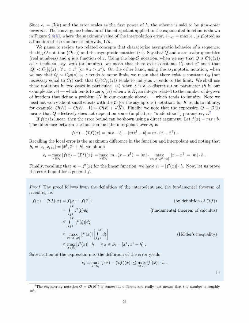
Proof. The proof follows from the definition of the interpolant and the fundamental theorem ofcalculus, i.e.

f(x)− (If)(x) = f(x)− f(x1) (by definition of (If))

=

∫ x

x1f ′(ξ)dξ (fundamental theorem of calculus)

≤∫ x

x1|f ′(ξ)|dξ

≤ maxx∈[x1,x]

|f ′(x)|∣∣∣∣∫ x

x1dξ

∣∣∣∣ (Holder’s inequality)

≤ maxx∈Si|f ′(x)| · h, ∀ x ∈ Si = [x1, x1 + h] .

Substitution of the expression into the definition of the error yields

ei ≡ maxx∈Si|f(x)− (If)(x)| ≤ max

x∈Si|f ′(x)| · h .

2The engineering notation Q = O(103) is somewhat different and really just means that the number is roughly103.

21

0 0.2 0.4 0.6 0.8 1

0

0.2

0.4

0.6

0.8

1

interpolantinterpolation pointsfunction

(a) interpolant

1 2 4 8 16 3210

−2

10−1

100

101

1/h

ma

x(e

i)

(b) error

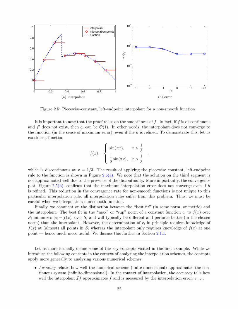
Figure 2.5: Piecewise-constant, left-endpoint interpolant for a non-smooth function.

It is important to note that the proof relies on the smoothness of f . In fact, if f is discontinuousand f ′ does not exist, then ei can be O(1). In other words, the interpolant does not converge tothe function (in the sense of maximum error), even if the h is refined. To demonstrate this, let usconsider a function

f(x) =

sin(πx), x ≤ 1

31

2sin(πx), x >

1

3

,

which is discontinuous at x = 1/3. The result of applying the piecewise constant, left-endpointrule to the function is shown in Figure 2.5(a). We note that the solution on the third segment isnot approximated well due to the presence of the discontinuity. More importantly, the convergenceplot, Figure 2.5(b), confirms that the maximum interpolation error does not converge even if his refined. This reduction in the convergence rate for non-smooth functions is not unique to thisparticular interpolation rule; all interpolation rules suffer from this problem. Thus, we must becareful when we interpolate a non-smooth function.

Finally, we comment on the distinction between the “best fit” (in some norm, or metric) andthe interpolant. The best fit in the “max” or “sup” norm of a constant function ci to f(x) overSi minimizes |ci − f(x)| over Si and will typically be different and perforce better (in the chosennorm) than the interpolant. However, the determination of ci in principle requires knowledge off(x) at (almost) all points in Si whereas the interpolant only requires knowledge of f(x) at onepoint — hence much more useful. We discuss this further in Section 2.1.1.

·Let us more formally define some of the key concepts visited in the first example. While we

introduce the following concepts in the context of analyzing the interpolation schemes, the conceptsapply more generally to analyzing various numerical schemes.

• Accuracy relates how well the numerical scheme (finite-dimensional) approximates the con-tinuous system (infinite-dimensional). In the context of interpolation, the accuracy tells howwell the interpolant If approximates f and is measured by the interpolation error, emax.

22

• Convergence is the property that the error vanishes as the discretization is refined, i.e.

emax → 0 as h→ 0 .

A convergent scheme can achieve any desired accuracy (error) in infinite prediction arith-metics by choosing h sufficiently small. The piecewise-constant, left-endpoint interpolant isa convergent scheme, because emax = O(h), and emax → 0 as h→ 0.

• Convergence rate is the power p such that

emax ≤ Chp as h→ 0 ,

where C is a constant independent of h. The scheme is first-order accurate for p = 1, second-order accurate for p = 2, and so on. The piecewise-constant, left-endpoint interpolant isfirst-order accurate because emax = Ch1. Note here p is fixed and the convergence (withnumber of intervals) is thus algebraic.

Note that typically as h→ 0 we obtain not a bound but in fact asymptotic behavior: emax ∼Chp or equivalently, emax/(Ch

p) → 1, as h → 0. Taking the logarithm of emax ∼ Chp,we obtain ln(emax) ∼ lnC + p lnh. Thus, a log-log plot is a convenient means of finding pempirically.

• Resolution is the characteristic length hcrit for any particular problem (described by f) forwhich we see the asymptotic convergence rate for h ≤ hcrit. Convergence plot in Figure 2.4(b)shows that the piecewise-constant, left-endpoint interpolant achieves the asymptotic conver-gence rate of 1 with respect to h for h ≤ 1/2; note that the slope from h = 1 to h = 1/2is lower than unity. Thus, hcrit for the interpolation scheme applied to f(x) = exp(x) isapproximately 1/2.

• Computational cost or operation count is the number of floating point operations (FLOPs3) tocompute Ih. As h→ 0, the number of FLOPs approaches∞. The scaling of the computationcost with the size of the problem is referred to as computational complexity . The actual run-time of computation is a function of the computational cost and the hardware. The cost ofconstructing the piecewise-constant, left end point interpolant is proportional to the numberof segments. Thus, the cost scales linearly with N , and the scheme is said to have linearcomplexity.

• Memory or storage is the number of floating point numbers that must be stored at any pointduring execution.

We note that the above properties characterize a scheme in infinite precision representation andarithmetic. Precision is related to machine precision, floating point number truncation, roundingand arithmetic errors, etc, all of which are absent in infinite-precision arithmetics.

We also note that there are two conflicting demands; the accuracy of the scheme increaseswith decreasing h (assuming the scheme is convergent), but the computational cost increases withdecreasing h. Intuitively, this always happen because the dimension of the discrete approximationmust be increased to better approximate the continuous system. However, some schemes producelower error for the same computational cost than other schemes. The performance of a numericalscheme is assessed in terms of the accuracy it delivers for a given computational cost.

We will now visit several other interpolation schemes and characterize the schemes using theabove properties.

3Not to be confused with the FLOPS (floating point operations per second), which is often used to measure theperformance of a computational hardware.

23

0 0.2 0.4 0.6 0.8 10.5

1

1.5

2

2.5

3

interpolant

interpolation points

function

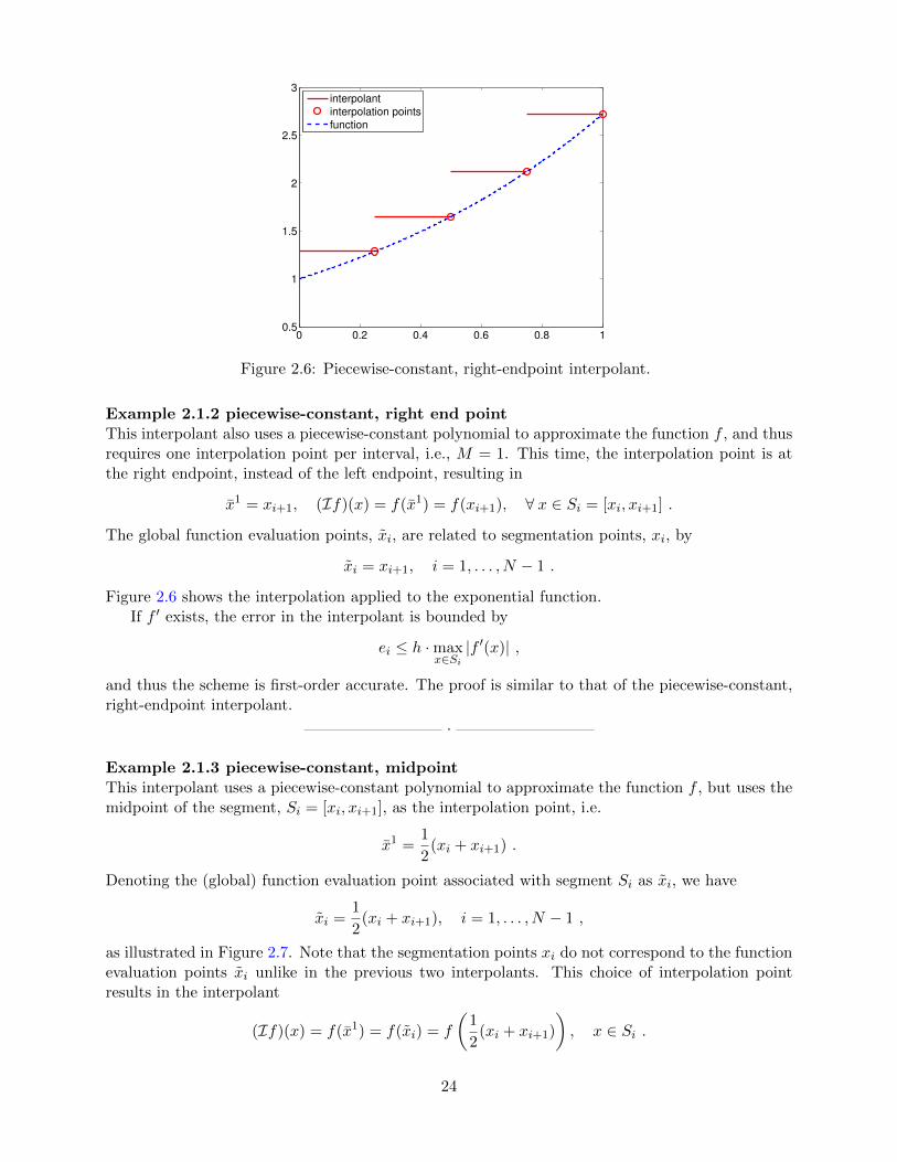
Figure 2.6: Piecewise-constant, right-endpoint interpolant.

Example 2.1.2 piecewise-constant, right end pointThis interpolant also uses a piecewise-constant polynomial to approximate the function f , and thusrequires one interpolation point per interval, i.e., M = 1. This time, the interpolation point is atthe right endpoint, instead of the left endpoint, resulting in

x1 = xi+1, (If)(x) = f(x1) = f(xi+1), ∀ x ∈ Si = [xi, xi+1] .

The global function evaluation points, xi, are related to segmentation points, xi, by

xi = xi+1, i = 1, . . . , N − 1 .

Figure 2.6 shows the interpolation applied to the exponential function.If f ′ exists, the error in the interpolant is bounded by

ei ≤ h ·maxx∈Si|f ′(x)| ,

and thus the scheme is first-order accurate. The proof is similar to that of the piecewise-constant,right-endpoint interpolant.

·

Example 2.1.3 piecewise-constant, midpointThis interpolant uses a piecewise-constant polynomial to approximate the function f , but uses themidpoint of the segment, Si = [xi, xi+1], as the interpolation point, i.e.

x1 =1

2(xi + xi+1) .

Denoting the (global) function evaluation point associated with segment Si as xi, we have

xi =1

2(xi + xi+1), i = 1, . . . , N − 1 ,

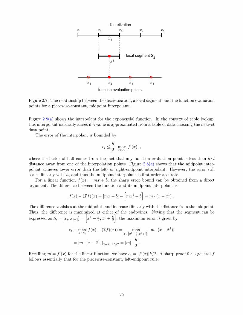
as illustrated in Figure 2.7. Note that the segmentation points xi do not correspond to the functionevaluation points xi unlike in the previous two interpolants. This choice of interpolation pointresults in the interpolant

(If)(x) = f(x1) = f(xi) = f

(1

2(xi + xi+1)

), x ∈ Si .

24

x1

x2

x3

x4

x5

S2

discretization

x1

local segment S2

x1

x2

x3

x4

function evaluation points

Figure 2.7: The relationship between the discretization, a local segment, and the function evaluationpoints for a piecewise-constant, midpoint interpolant.

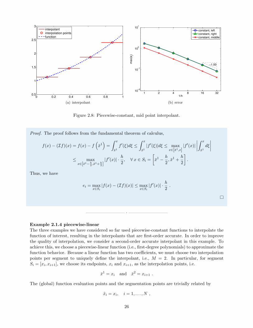
Figure 2.8(a) shows the interpolant for the exponential function. In the context of table lookup,this interpolant naturally arises if a value is approximated from a table of data choosing the nearestdata point.

The error of the interpolant is bounded by

ei ≤h

2·maxx∈Si|f ′(x)| ,

where the factor of half comes from the fact that any function evaluation point is less than h/2distance away from one of the interpolation points. Figure 2.8(a) shows that the midpoint inter-polant achieves lower error than the left- or right-endpoint interpolant. However, the error stillscales linearly with h, and thus the midpoint interpolant is first-order accurate.

For a linear function f(x) = mx + b, the sharp error bound can be obtained from a directargument. The difference between the function and its midpoint interpolant is

f(x)− (If)(x) = [mx+ b]−[mx1 + b

]= m · (x− x1) .

The difference vanishes at the midpoint, and increases linearly with the distance from the midpoint.Thus, the difference is maximized at either of the endpoints. Noting that the segment can be

expressed as Si = [xi, xi+1] =[x1 − h

2 , x1 + h

2

], the maximum error is given by

ei ≡ maxx∈Si

(f(x)− (If)(x)) = maxx∈[x1−h2 ,x1+h

2 ]|m · (x− x1)|

= |m · (x− x1)|x=x1±h/2 = |m| · h2.

Recalling m = f ′(x) for the linear function, we have ei = |f ′(x)|h/2. A sharp proof for a general ffollows essentially that for the piecewise-constant, left-endpoint rule.

25

0 0.2 0.4 0.6 0.8 10.5

1

1.5

2

2.5

3

interpolant

interpolation points

function

(a) interpolant

1 2 4 8 16 3210

−2

10−1

100

101

−1.00

1/h

max(e

i)

constant, left

constant, right

constant, middle

(b) error

Figure 2.8: Piecewise-constant, mid point interpolant.

Proof. The proof follows from the fundamental theorem of calculus,

f(x)− (If)(x) = f(x)− f(x1)

=

∫ x

x1f ′(ξ)dξ ≤

∫ x

x1|f ′(ξ)|dξ ≤ max

x∈[x1,x]|f ′(x)|

∣∣∣∣∫ x

x1dξ

∣∣∣∣≤ max

x∈[x1−h2 ,x1+h2 ]|f ′(x)| · h

2, ∀ x ∈ Si =

[x1 − h

2, x1 +

h

2

].

Thus, we have

ei = maxx∈Si|f(x)− (If)(x)| ≤ max

x∈Si|f ′(x)| · h

2.

·

Example 2.1.4 piecewise-linearThe three examples we have considered so far used piecewise-constant functions to interpolate thefunction of interest, resulting in the interpolants that are first-order accurate. In order to improvethe quality of interpolation, we consider a second-order accurate interpolant in this example. Toachieve this, we choose a piecewise-linear function (i.e., first-degree polynomials) to approximate thefunction behavior. Because a linear function has two coefficients, we must choose two interpolationpoints per segment to uniquely define the interpolant, i.e., M = 2. In particular, for segmentSi = [xi, xi+1], we choose its endpoints, xi and xi+1, as the interpolation points, i.e.

x1 = xi and x2 = xi+1 .

The (global) function evaluation points and the segmentation points are trivially related by

xi = xi, i = 1, . . . , N ,

26

x1

x2

x3

x4

x5

S2

discretization

x1 x2

local segment S2

x1

x2

x3

x4

x5

function evaluation points

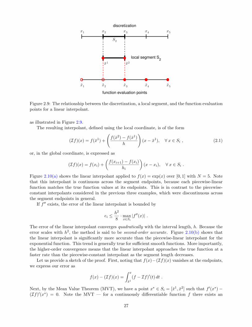
Figure 2.9: The relationship between the discretization, a local segment, and the function evaluationpoints for a linear interpolant.

as illustrated in Figure 2.9.The resulting interpolant, defined using the local coordinate, is of the form

(If)(x) = f(x1) +

(f(x2)− f(x1)

h

)(x− x1), ∀ x ∈ Si , (2.1)

or, in the global coordinate, is expressed as

(If)(x) = f(xi) +

(f(xi+1)− f(xi)

hi

)(x− xi), ∀ x ∈ Si .

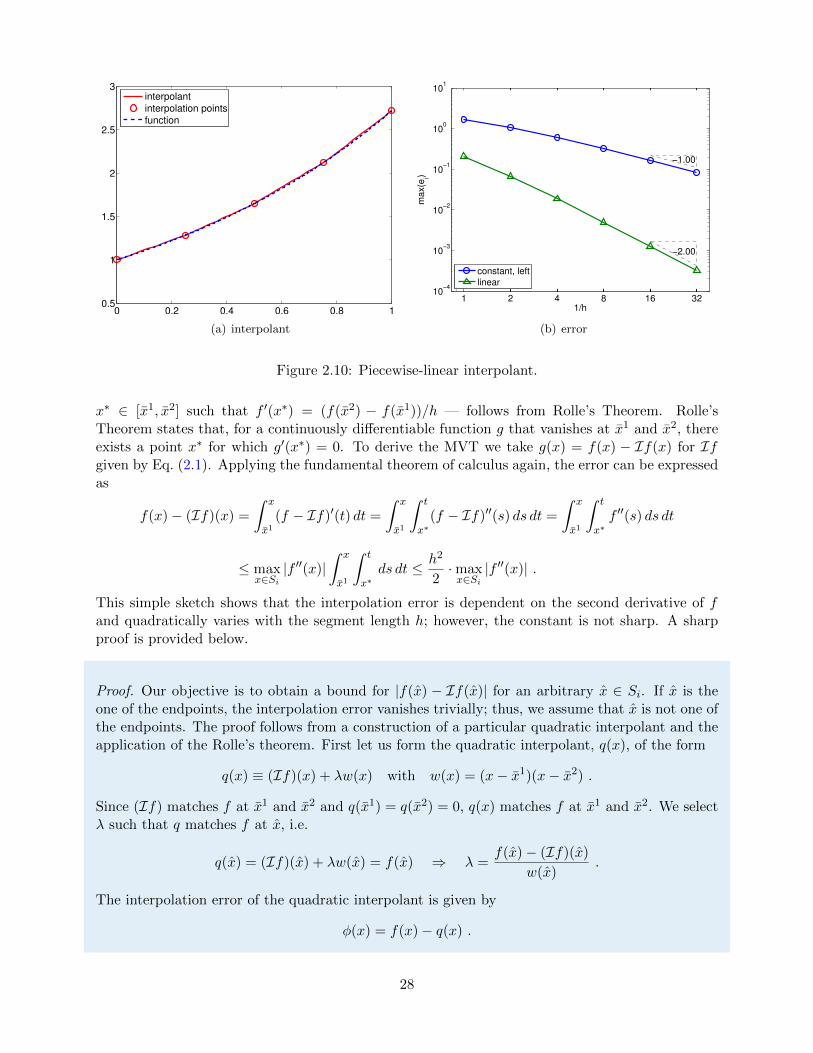
Figure 2.10(a) shows the linear interpolant applied to f(x) = exp(x) over [0, 1] with N = 5. Notethat this interpolant is continuous across the segment endpoints, because each piecewise-linearfunction matches the true function values at its endpoints. This is in contrast to the piecewise-constant interpolants considered in the previous three examples, which were discontinuous acrossthe segment endpoints in general.

If f ′′ exists, the error of the linear interpolant is bounded by

ei ≤h2

8·maxx∈Si|f ′′(x)| .

The error of the linear interpolant converges quadratically with the interval length, h. Because theerror scales with h2, the method is said to be second-order accurate. Figure 2.10(b) shows thatthe linear interpolant is significantly more accurate than the piecewise-linear interpolant for theexponential function. This trend is generally true for sufficient smooth functions. More importantly,the higher-order convergence means that the linear interpolant approaches the true function at afaster rate than the piecewise-constant interpolant as the segment length decreases.

Let us provide a sketch of the proof. First, noting that f(x)−(If)(x) vanishes at the endpoints,we express our error as

f(x)− (If)(x) =

∫ x

x1(f − If)′(t) dt .

Next, by the Mean Value Theorem (MVT), we have a point x∗ ∈ Si = [x1, x2] such that f ′(x∗) −(If)′(x∗) = 0. Note the MVT — for a continuously differentiable function f there exists an

27

0 0.2 0.4 0.6 0.8 10.5

1

1.5

2

2.5

3

interpolant

interpolation points

function

(a) interpolant

1 2 4 8 16 3210

−4

10−3

10−2

10−1

100

101

−1.00

−2.00

1/h

max(e

i)

constant, left

linear

(b) error

Figure 2.10: Piecewise-linear interpolant.

x∗ ∈ [x1, x2] such that f ′(x∗) = (f(x2) − f(x1))/h — follows from Rolle’s Theorem. Rolle’sTheorem states that, for a continuously differentiable function g that vanishes at x1 and x2, thereexists a point x∗ for which g′(x∗) = 0. To derive the MVT we take g(x) = f(x) − If(x) for Ifgiven by Eq. (2.1). Applying the fundamental theorem of calculus again, the error can be expressedas

f(x)− (If)(x) =

∫ x

x1(f − If)′(t) dt =

∫ x

x1

∫ t

x∗(f − If)′′(s) ds dt =

∫ x

x1

∫ t

x∗f ′′(s) ds dt

≤ maxx∈Si|f ′′(x)|

∫ x

x1

∫ t

x∗ds dt ≤ h2

2·maxx∈Si|f ′′(x)| .

This simple sketch shows that the interpolation error is dependent on the second derivative of fand quadratically varies with the segment length h; however, the constant is not sharp. A sharpproof is provided below.

Proof. Our objective is to obtain a bound for |f(x) − If(x)| for an arbitrary x ∈ Si. If x is theone of the endpoints, the interpolation error vanishes trivially; thus, we assume that x is not one ofthe endpoints. The proof follows from a construction of a particular quadratic interpolant and theapplication of the Rolle’s theorem. First let us form the quadratic interpolant, q(x), of the form

q(x) ≡ (If)(x) + λw(x) with w(x) = (x− x1)(x− x2) .

Since (If) matches f at x1 and x2 and q(x1) = q(x2) = 0, q(x) matches f at x1 and x2. We selectλ such that q matches f at x, i.e.

q(x) = (If)(x) + λw(x) = f(x) ⇒ λ =f(x)− (If)(x)

w(x).

The interpolation error of the quadratic interpolant is given by

φ(x) = f(x)− q(x) .

28

Because q is the quadratic interpolant of f defined by the interpolation points x1, x2, and x, φ hasthree zeros in Si. By Rolle’s theorem, φ′ has two zeros in Si. Again, by Rolle’s theorem, φ′′ hasone zero in Si. Let this zero be denoted by ξ, i.e., φ′′(ξ) = 0. Evaluation of φ′′(ξ) yields

0 = φ′′(ξ) = f ′′(ξ)− q′′(ξ) = f ′′(ξ)− (If)′′(ξ)− λw′′(ξ) = f ′′(ξ)− 2λ ⇒ λ =1

2f ′′(ξ) .

Evaluating φ(x), we obtain

0 = φ(x) = f(x)− (If)(x)− 1

2f ′′(ξ)w(x) (2.2)

f(x)− (If)(x) =1

2f ′′(ξ)(x− x1)(x− x2) . (2.3)

The function is maximized for x∗ = (x1 + x2)/2, which yields

f(x)− (If)(x) ≤ 1

8f ′′(ξ)(x2 − x1)2 =

1

8h2f ′′(ξ), ∀ x ∈ [x1, x2]

Since ξ ∈ Si, it follows that,

ei = maxx∈Si|f(x)− (If)(x)| ≤ 1

8h2f ′′(ξ) ≤ 1

8h2 max

x∈Si|f ′′(x)| .

·

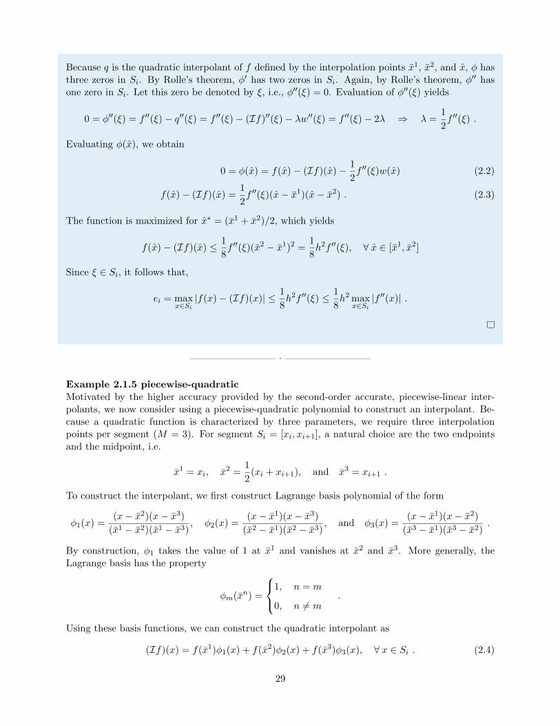
Example 2.1.5 piecewise-quadraticMotivated by the higher accuracy provided by the second-order accurate, piecewise-linear inter-polants, we now consider using a piecewise-quadratic polynomial to construct an interpolant. Be-cause a quadratic function is characterized by three parameters, we require three interpolationpoints per segment (M = 3). For segment Si = [xi, xi+1], a natural choice are the two endpointsand the midpoint, i.e.

x1 = xi, x2 =1

2(xi + xi+1), and x3 = xi+1 .

To construct the interpolant, we first construct Lagrange basis polynomial of the form

φ1(x) =(x− x2)(x− x3)

(x1 − x2)(x1 − x3), φ2(x) =

(x− x1)(x− x3)

(x2 − x1)(x2 − x3), and φ3(x) =

(x− x1)(x− x2)

(x3 − x1)(x3 − x2).

By construction, φ1 takes the value of 1 at x1 and vanishes at x2 and x3. More generally, theLagrange basis has the property

φm(xn) =

1, n = m

0, n 6= m.

Using these basis functions, we can construct the quadratic interpolant as

(If)(x) = f(x1)φ1(x) + f(x2)φ2(x) + f(x3)φ3(x), ∀ x ∈ Si . (2.4)

29

0 0.2 0.4 0.6 0.8 10.5

1

1.5

2

2.5

3

interpolant

interpolation points

function

(a) interpolant

1 2 4 8 16 3210

−8

10−6

10−4

10−2

100

102

−1.00

−2.00

−3.00

1/h

max(e

i)

constant, left

linear

quadratic

(b) error

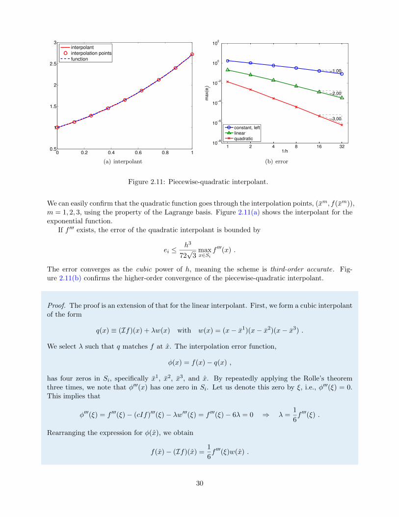
Figure 2.11: Piecewise-quadratic interpolant.

We can easily confirm that the quadratic function goes through the interpolation points, (xm, f(xm)),m = 1, 2, 3, using the property of the Lagrange basis. Figure 2.11(a) shows the interpolant for theexponential function.

If f ′′′ exists, the error of the quadratic interpolant is bounded by

ei ≤h3

72√

3maxx∈Si

f ′′′(x) .

The error converges as the cubic power of h, meaning the scheme is third-order accurate. Fig-ure 2.11(b) confirms the higher-order convergence of the piecewise-quadratic interpolant.

Proof. The proof is an extension of that for the linear interpolant. First, we form a cubic interpolantof the form

q(x) ≡ (If)(x) + λw(x) with w(x) = (x− x1)(x− x2)(x− x3) .

We select λ such that q matches f at x. The interpolation error function,

φ(x) = f(x)− q(x) ,

has four zeros in Si, specifically x1, x2, x3, and x. By repeatedly applying the Rolle’s theoremthree times, we note that φ′′′(x) has one zero in Si. Let us denote this zero by ξ, i.e., φ′′′(ξ) = 0.This implies that

φ′′′(ξ) = f ′′′(ξ)− (cIf)′′′(ξ)− λw′′′(ξ) = f ′′′(ξ)− 6λ = 0 ⇒ λ =1

6f ′′′(ξ) .

Rearranging the expression for φ(x), we obtain

f(x)− (If)(x) =1

6f ′′′(ξ)w(x) .

30

0 0.2 0.4 0.6 0.8 1

0

0.2

0.4

0.6

0.8

1

interpolantinterpolation pointsfunction

(a) interpolant

1 2 4 8 16 3210

−2

10−1

100

101

1/h

max(e

i)

constant, left

linear

quadratic

(b) error

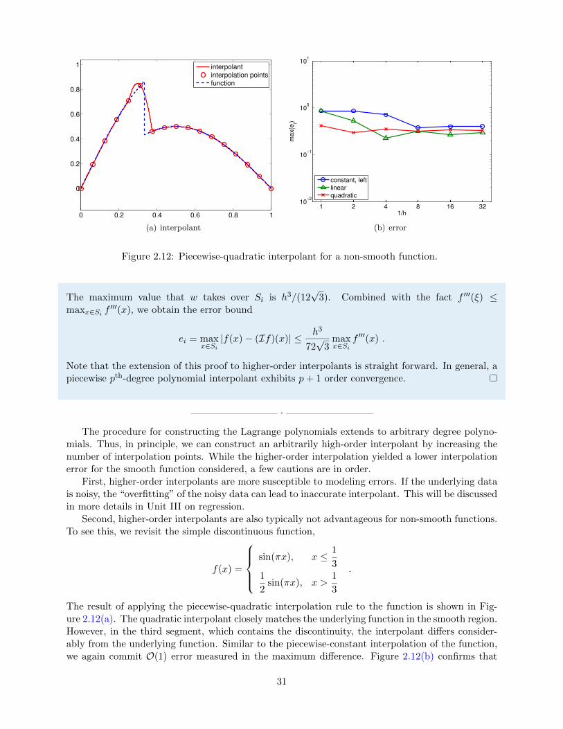
Figure 2.12: Piecewise-quadratic interpolant for a non-smooth function.

The maximum value that w takes over Si is h3/(12√

3). Combined with the fact f ′′′(ξ) ≤maxx∈Si f

′′′(x), we obtain the error bound

ei = maxx∈Si|f(x)− (If)(x)| ≤ h3

72√

3maxx∈Si

f ′′′(x) .

Note that the extension of this proof to higher-order interpolants is straight forward. In general, apiecewise pth-degree polynomial interpolant exhibits p+ 1 order convergence.

·The procedure for constructing the Lagrange polynomials extends to arbitrary degree polyno-

mials. Thus, in principle, we can construct an arbitrarily high-order interpolant by increasing thenumber of interpolation points. While the higher-order interpolation yielded a lower interpolationerror for the smooth function considered, a few cautions are in order.

First, higher-order interpolants are more susceptible to modeling errors. If the underlying datais noisy, the “overfitting” of the noisy data can lead to inaccurate interpolant. This will be discussedin more details in Unit III on regression.

Second, higher-order interpolants are also typically not advantageous for non-smooth functions.To see this, we revisit the simple discontinuous function,

f(x) =

sin(πx), x ≤ 1

31

2sin(πx), x >

1

3

.

The result of applying the piecewise-quadratic interpolation rule to the function is shown in Fig-ure 2.12(a). The quadratic interpolant closely matches the underlying function in the smooth region.However, in the third segment, which contains the discontinuity, the interpolant differs consider-ably from the underlying function. Similar to the piecewise-constant interpolation of the function,we again commit O(1) error measured in the maximum difference. Figure 2.12(b) confirms that

31

the higher-order interpolants do not perform any better than the piecewise-constant interpolantin the presence of discontinuity. Formally, we can show that the maximum-error convergence ofany interpolation scheme can be no better than hr, where r is the highest-order derivative thatis defined everywhere in the domain. In the presence of a discontinuity, r = 0, and we observeO(hr) = O(1) convergence (i.e., no convergence).

Third, for a very high-order polynomials, the interpolation points must be chosen carefully toachieve a good result. In particular, the uniform distribution suffers from the behavior knownas Runge’s phenomenon, where the interpolant exhibits excessive oscillation even if the underlyingfunction is smooth. The spurious oscillation can be minimized by clustering the interpolation pointsnear the segment endpoints, e.g., Chebyshev nodes.

Advanced Material

2.1.1 Best Fit vs. Interpolation: Polynomials of Degree n

We will study in more details how the choice of interpolation points affect the quality of a polynomialinterpolant. For convenience, let us denote the space of nth-degree polynomials on segment S byPn(S). For consistency, we will denote nth-degree polynomial interpolant of f , which is definedby n + 1 interpolation points {xm}n+1

m=1, by Inf . We will compare the quality of the interpolantwith the “best” n+ 1 degree polynomial. We will define “best” in the infinity norm, i.e., the bestpolynomial v∗ ∈ Pn(S) satisfies

maxx∈S|f(x)− v∗(x)| ≤ max

x∈S|f(x)− v(x)| , ∀ v ∈ Pn(x) .

In some sense, the polynomial v∗ fits the function f as closely as possible. Then, the quality ofa nth-degree interpolant can be assessed by measuring how close it is to v∗. More precisely, wequantify its quality by comparing the maximum error of the interpolant with that of the bestpolynomial, i.e.

maxx∈S|f(x)− (If)(x)| ≤ (1 + Λ({xm}n+1

m=1)) maxx∈S|f(x)− v∗(x)| ,

where the constant Λ is called the Lebesgue constant. Clearly, a smaller Lebesgue constant impliessmaller error, so higher the quality of the interpolant. At the same time, Λ ≥ 0 because themaximum error in the interpolant cannot be better than that of the “best” function, which bydefinition minimizes the maximum error. In fact, the Lebesgue constant is given by

Λ({xm}n+1

m=1

)= max

x∈S

n+1∑m=1

|φm(x)| ,

where φm, m = 1, . . . , n+ 1, are the Lagrange bases functions defined by the nodes {xm}n+1m=1.

Proof. We first express the interpolation error in the infinity norm as the sum of two contributions

maxx∈S|f(x)− (If)(x)| ≤ max

x∈S|f(x)− v∗(x) + v∗(x)− (If)(x)|

≤ maxx∈S|f(x)− v∗(x)|+ max

x∈S|v∗(x)− (If)(x)|.

32

Noting that the functions in the second term are polynomial, we express them in terms of theLagrange basis φm, m = 1, . . . , n,

maxx∈S|v∗(x)− (If)(x)| = max

x∈S

∣∣∣∣∣∣n+1∑m=1

(v∗(xm)− (If)(xm))φm(x)

∣∣∣∣∣∣≤ max

x∈S

∣∣∣∣∣∣ maxm=1,...,n+1

|v∗(xm)− (If)(xm)| ·n+1∑m=1

|φm(x)|

∣∣∣∣∣∣= max

m=1,...,n+1|v∗(xm)− (If)(xm)| ·max

x∈S

n+1∑m=1

|φm(x)| .

Because If is an interpolant, we have f(xm) = (If)(xm), m = 1, . . . , n+1. Moreover, we recognizethat the second term is the expression for Lebesgue constant. Thus, we have

maxx∈S|v∗(x)− (If)(x)| ≤ max

m=1,...,n+1|v∗(xm)− f(xm)| · Λ

≤ maxx∈S|v∗(x)− f(x)|Λ .

where the last inequality follows from recognizing xm ∈ S, m = 1, . . . , n+1. Thus, the interpolationerror in the maximum norm is bounded by

maxx∈S|f(x)− (If)(x)| ≤ max

x∈S|v∗(x)− f(x)|+ max

x∈S|v∗(x)− f(x)|Λ

≤ (1 + Λ) maxx∈S|v∗(x)− f(x)| ,

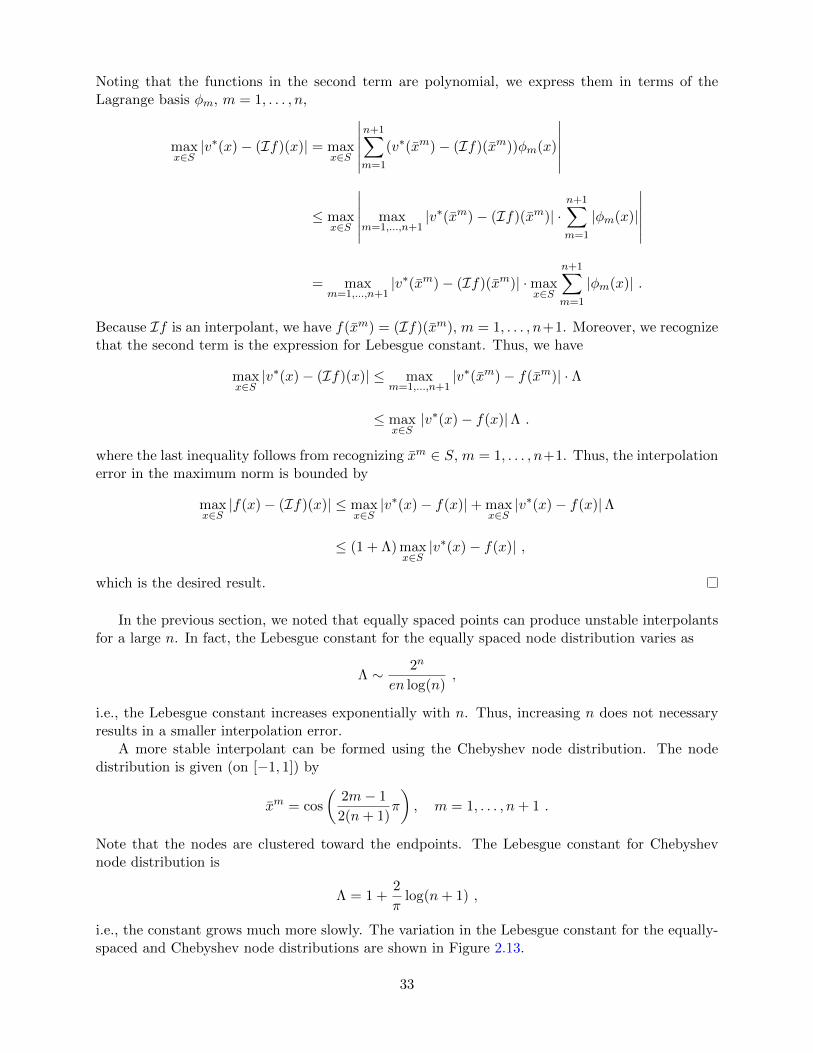
which is the desired result.

In the previous section, we noted that equally spaced points can produce unstable interpolantsfor a large n. In fact, the Lebesgue constant for the equally spaced node distribution varies as

Λ ∼ 2n

en log(n),

i.e., the Lebesgue constant increases exponentially with n. Thus, increasing n does not necessaryresults in a smaller interpolation error.

A more stable interpolant can be formed using the Chebyshev node distribution. The nodedistribution is given (on [−1, 1]) by

xm = cos

(2m− 1

2(n+ 1)π

), m = 1, . . . , n+ 1 .

Note that the nodes are clustered toward the endpoints. The Lebesgue constant for Chebyshevnode distribution is

Λ = 1 +2

πlog(n+ 1) ,

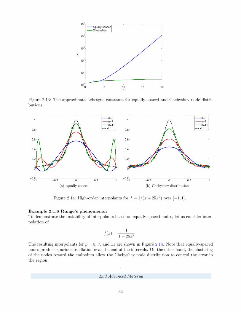
i.e., the constant grows much more slowly. The variation in the Lebesgue constant for the equally-spaced and Chebyshev node distributions are shown in Figure 2.13.

33

0 5 10 15 2010

0

101

102

103

104

105

n

Λ

equally spaced

Chebyshev

Figure 2.13: The approximate Lebesgue constants for equally-spaced and Chebyshev node distri-butions.

−1 −0.5 0 0.5 1−0.2

0

0.2

0.4

0.6

0.8

1

n=5

n=7

n=11

f

(a) equally spaced

−1 −0.5 0 0.5 1−0.2

0

0.2

0.4

0.6

0.8

1

n=5

n=7

n=11

f

(b) Chebyshev distribution

Figure 2.14: High-order interpolants for f = 1/(x+ 25x2) over [−1, 1].

Example 2.1.6 Runge’s phenomenonTo demonstrate the instability of interpolants based on equally-spaced nodes, let us consider inter-polation of

f(x) =1

1 + 25x2.

The resulting interpolants for p = 5, 7, and 11 are shown in Figure 2.14. Note that equally-spacednodes produce spurious oscillation near the end of the intervals. On the other hand, the clusteringof the nodes toward the endpoints allow the Chebyshev node distribution to control the error inthe region.

·

End Advanced Material

34

R1

R2

R3

Ri

(a) mesh

Ri

x1

x2

x3

(b) triangle Ri

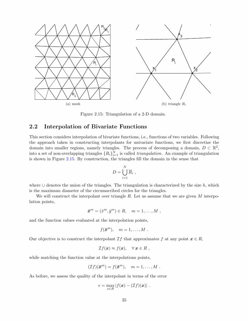
Figure 2.15: Triangulation of a 2-D domain.

2.2 Interpolation of Bivariate Functions

This section considers interpolation of bivariate functions, i.e., functions of two variables. Followingthe approach taken in constructing interpolants for univariate functions, we first discretize thedomain into smaller regions, namely triangles. The process of decomposing a domain, D ⊂ R2,into a set of non-overlapping triangles {Ri}Ni=1 is called triangulation. An example of triangulationis shown in Figure 2.15. By construction, the triangles fill the domain in the sense that

D =N⋃i=1

Ri ,

where ∪ denotes the union of the triangles. The triangulation is characterized by the size h, whichis the maximum diameter of the circumscribed circles for the triangles.

We will construct the interpolant over triangle R. Let us assume that we are given M interpo-lation points,

xm = (xm, ym) ∈ R, m = 1, . . . ,M ,

and the function values evaluated at the interpolation points,

f(xm), m = 1, . . . ,M .

Our objective is to construct the interpolant If that approximates f at any point x ∈ R,

If(x) ≈ f(x), ∀ x ∈ R ,

while matching the function value at the interpolations points,

(If)(xm) = f(xm), m = 1, . . . ,M .

As before, we assess the quality of the interpolant in terms of the error

e = maxx∈R|f(x)− (If)(x)| .

35

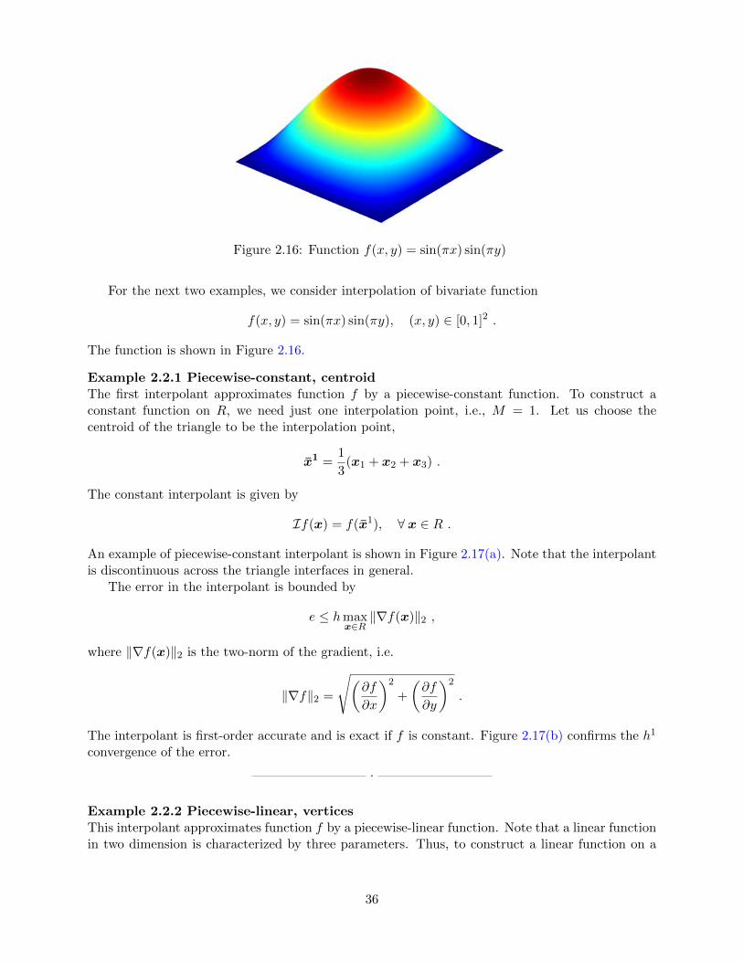
Figure 2.16: Function f(x, y) = sin(πx) sin(πy)

For the next two examples, we consider interpolation of bivariate function

f(x, y) = sin(πx) sin(πy), (x, y) ∈ [0, 1]2 .

The function is shown in Figure 2.16.

Example 2.2.1 Piecewise-constant, centroidThe first interpolant approximates function f by a piecewise-constant function. To construct aconstant function on R, we need just one interpolation point, i.e., M = 1. Let us choose thecentroid of the triangle to be the interpolation point,

x1 =1

3(x1 + x2 + x3) .

The constant interpolant is given by

If(x) = f(x1), ∀ x ∈ R .

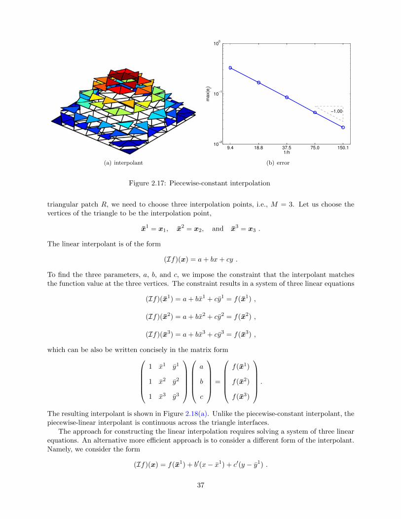
An example of piecewise-constant interpolant is shown in Figure 2.17(a). Note that the interpolantis discontinuous across the triangle interfaces in general.

The error in the interpolant is bounded by

e ≤ hmaxx∈R‖∇f(x)‖2 ,

where ‖∇f(x)‖2 is the two-norm of the gradient, i.e.

‖∇f‖2 =

√(∂f

∂x

)2

+

(∂f

∂y

)2

.

The interpolant is first-order accurate and is exact if f is constant. Figure 2.17(b) confirms the h1

convergence of the error.

·

Example 2.2.2 Piecewise-linear, verticesThis interpolant approximates function f by a piecewise-linear function. Note that a linear functionin two dimension is characterized by three parameters. Thus, to construct a linear function on a

36

(a) interpolant

9.4 18.8 37.5 75.0 150.110

−2

10−1

100

−1.00

1/h

ma

x(e

i)

(b) error

Figure 2.17: Piecewise-constant interpolation

triangular patch R, we need to choose three interpolation points, i.e., M = 3. Let us choose thevertices of the triangle to be the interpolation point,

x1 = x1, x2 = x2, and x3 = x3 .

The linear interpolant is of the form

(If)(x) = a+ bx+ cy .

To find the three parameters, a, b, and c, we impose the constraint that the interpolant matchesthe function value at the three vertices. The constraint results in a system of three linear equations

(If)(x1) = a+ bx1 + cy1 = f(x1) ,

(If)(x2) = a+ bx2 + cy2 = f(x2) ,

(If)(x3) = a+ bx3 + cy3 = f(x3) ,

which can be also be written concisely in the matrix form1 x1 y1

1 x2 y2

1 x3 y3

a

b

c

=

f(x1)

f(x2)

f(x3)

.

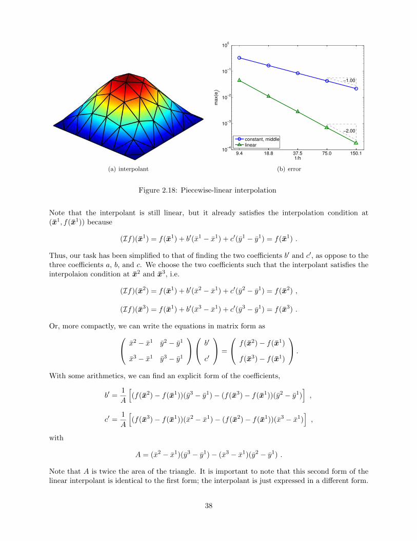
The resulting interpolant is shown in Figure 2.18(a). Unlike the piecewise-constant interpolant, thepiecewise-linear interpolant is continuous across the triangle interfaces.

The approach for constructing the linear interpolation requires solving a system of three linearequations. An alternative more efficient approach is to consider a different form of the interpolant.Namely, we consider the form

(If)(x) = f(x1) + b′(x− x1) + c′(y − y1) .

37

(a) interpolant

9.4 18.8 37.5 75.0 150.110

−4

10−3

10−2

10−1

100

−1.00

−2.00

1/h

max(e

i)

constant, middle

linear

(b) error

Figure 2.18: Piecewise-linear interpolation

Note that the interpolant is still linear, but it already satisfies the interpolation condition at(x1, f(x1)) because

(If)(x1) = f(x1) + b′(x1 − x1) + c′(y1 − y1) = f(x1) .

Thus, our task has been simplified to that of finding the two coefficients b′ and c′, as oppose to thethree coefficients a, b, and c. We choose the two coefficients such that the interpolant satisfies theinterpolaion condition at x2 and x3, i.e.

(If)(x2) = f(x1) + b′(x2 − x1) + c′(y2 − y1) = f(x2) ,

(If)(x3) = f(x1) + b′(x3 − x1) + c′(y3 − y1) = f(x3) .

Or, more compactly, we can write the equations in matrix form as x2 − x1 y2 − y1

x3 − x1 y3 − y1

b′

c′

=

f(x2)− f(x1)

f(x3)− f(x1)

.

With some arithmetics, we can find an explicit form of the coefficients,

b′ =1

A

[(f(x2)− f(x1))(y3 − y1)− (f(x3)− f(x1))(y2 − y1)

],

c′ =1

A

[(f(x3)− f(x1))(x2 − x1)− (f(x2)− f(x1))(x3 − x1)

],

with

A = (x2 − x1)(y3 − y1)− (x3 − x1)(y2 − y1) .

Note that A is twice the area of the triangle. It is important to note that this second form of thelinear interpolant is identical to the first form; the interpolant is just expressed in a different form.

38

The error in the interpolant is governed by the Hessian of the function, i.e.

e ≤ Ch2‖∇2f‖F ,

where ‖∇2f‖F is the Frobenius norm of the Hessian matrix, i.e.

‖∇2f‖F =

√(∂2f

∂x2

)2

+

(∂2f

∂y2

)2

+ 2

(∂2f

∂x∂y

)2

.

Thus, the piecewise-linear interpolant is second-order accurate and is exact if f is linear. Theconvergence result shown in Figure 2.18(b) confirms the h2 convergence of the error.

·

39

40

Chapter 3

Differentiation

3.1 Differentiation of Univariate Functions

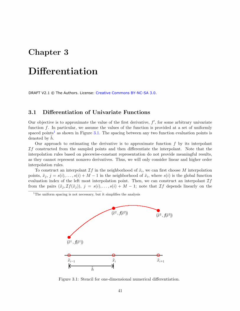
Our objective is to approximate the value of the first derivative, f ′, for some arbitrary univariatefunction f . In particular, we assume the values of the function is provided at a set of uniformlyspaced points1 as shown in Figure 3.1. The spacing between any two function evaluation points isdenoted by h.

Our approach to estimating the derivative is to approximate function f by its interpolantIf constructed from the sampled points and then differentiate the interpolant. Note that theinterpolation rules based on piecewise-constant representation do not provide meaningful results,as they cannot represent nonzero derivatives. Thus, we will only consider linear and higher orderinterpolation rules.

To construct an interpolant If in the neighborhood of xi, we can first choose M interpolationpoints, xj , j = s(i), . . . , s(i) + M − 1 in the neighborhood of xi, where s(i) is the global functionevaluation index of the left most interpolation point. Then, we can construct an interpolant Iffrom the pairs (xj , If(xj)), j = s(i), . . . , s(i) + M − 1; note that If depends linearly on the

1The uniform spacing is not necessary, but it simplifies the analysis

h

(x1 , f(x1))

(x2 , f(x2))(x3 , f(x3))

xixi−1 xi+1

Figure 3.1: Stencil for one-dimensional numerical differentiation.

41

DRAFT V2.1 © The Authors. License: Creative Commons BY-NC-SA 3.0.

function values, as we know from the Lagrange basis construction. As a result, the derivative of theinterpolant is also a linear function of f(xj), j = s(i), . . . , s(i) +M − 1. Specifically, our numericalapproximation to the derivative, f ′h(xi), is of the form

f ′h(xi) ≈s(i)+M−1∑j=s(i)

ωj(i)f(xj) ,

where ωj(i), j = 1, . . . ,M , are weights that are dependent on the choice of interpolant.These formulas for approximating the derivative are called finite difference formulas. In the

context of numerical differentiation, the set of function evaluation points used to approximate thederivative at xi is called numerical stencil . A scheme requiring M points to approximate thederivative has an M -point stencil. The scheme is said to be one-sided , if the derivative estimateonly involves the function values for either x ≥ xi or x ≤ xi. The computational cost of numericaldifferentiation is related to the size of stencil, M .

Throughout this chapter, we assess the quality of finite difference formulas in terms of the error

e ≡ |f ′(xi)− f ′h(xi)| .

Specifically, we are interested in analyzing the behavior of the error as our discretization is refined,i.e., as h decreases. Note that, because the interpolant, If , from which f ′h(xi) is constructedapproaches f as h → 0 for smooth functions, we also expect f ′h(xi) to approach f ′(xi) as h → 0.Thus, our goal is not just to verify that f ′(xi) approaches f(xi), but also to quantify how fast itconverges to the true value.

Let us provide a few examples of the differentiation rules.

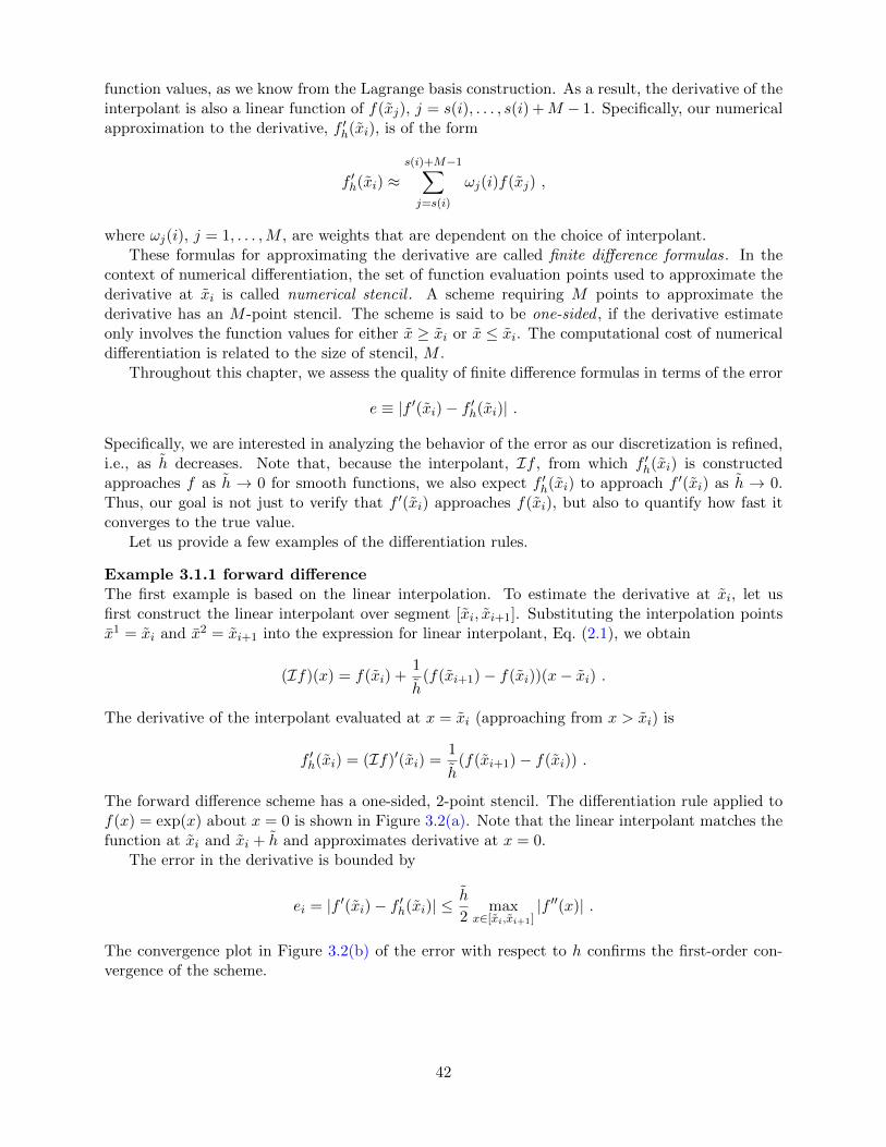
Example 3.1.1 forward differenceThe first example is based on the linear interpolation. To estimate the derivative at xi, let usfirst construct the linear interpolant over segment [xi, xi+1]. Substituting the interpolation pointsx1 = xi and x2 = xi+1 into the expression for linear interpolant, Eq. (2.1), we obtain

(If)(x) = f(xi) +1

h(f(xi+1)− f(xi))(x− xi) .

The derivative of the interpolant evaluated at x = xi (approaching from x > xi) is

f ′h(xi) = (If)′(xi) =1

h(f(xi+1)− f(xi)) .

The forward difference scheme has a one-sided, 2-point stencil. The differentiation rule applied tof(x) = exp(x) about x = 0 is shown in Figure 3.2(a). Note that the linear interpolant matches thefunction at xi and xi + h and approximates derivative at x = 0.

The error in the derivative is bounded by

ei = |f ′(xi)− f ′h(xi)| ≤h

2max

x∈[xi,xi+1]|f ′′(x)| .

The convergence plot in Figure 3.2(b) of the error with respect to h confirms the first-order con-vergence of the scheme.

42

−0.2 0 0.2 0.4 0.6 0.8 1 1.20.5

1

1.5

2

2.5

3

3.5

f’h(x)

f’(x)

interpolation points

function

(a) differentiation

2 4 8 16 32 6410

−3

10−2

10−1

100

−1.00

1/h

|f’−

f’h|

(b) error

Figure 3.2: Forward difference.

Proof. The proof of the error bound follows from Taylor expansion. Recall, assuming f ′′(x) isbounded in [xi, xi+1],

f(xi+1) = f(xi + h) = f(xi) + f ′(xi)h+1

2f ′′(ξ)h2 ,

for some ξ ∈ [xi, xi+1]. The derivative of the interpolant evaluated at x = xi can be expressed as

(If)′(xi) =1

h

(f(xi) + f ′(xi)h+

1

2f ′′(ξ)h2 − f(xi)

)= f ′(xi) +

1

2f ′′(ξ)h ,

and the error in the derivative is

|f ′(xi)− (If)′(xi)| =∣∣∣∣12f ′′(ξ)h

∣∣∣∣ ≤ 1

2h maxx∈[xi,xi+1]

|f ′′(x)| .

·

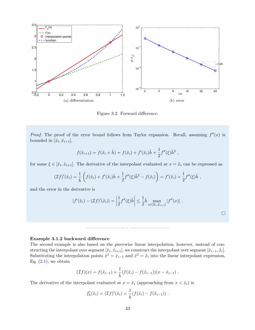
Example 3.1.2 backward differenceThe second example is also based on the piecewise linear interpolation; however, instead of con-structing the interpolant over segment [xi, xi+1], we construct the interpolant over segment [xi−1, xi].Substituting the interpolation points x1 = xi−1 and x2 = xi into the linear interpolant expression,Eq. (2.1), we obtain

(If)(x) = f(xi−1) +1

h(f(xi)− f(xi−1))(x− xi−1) .

The derivative of the interpolant evaluated at x = xi (approaching from x < xi) is

f ′h(xi) = (If)′(xi) =1

h(f(xi)− f(xi−1)) .

43

−1 −0.8 −0.6 −0.4 −0.2 0 0.2−0.2

0

0.2

0.4

0.6

0.8

1

1.2

1.4

f’h(x)

f’(x)

interpolation points

function

(a) differentiation (b) error

Figure 3.3: Backward difference.

The backward difference scheme has a one-sided, 2-point stencil. The differentiation rule appliedto f(x) = exp(x) about x = 0 is shown in Figure 3.3(a). The construction is similar to that of theforward difference, except that the interpolant matches the function at xi − h and xi.

The error in the derivative is bounded by

ei = |f ′(xi)− f ′h(xi)| ≤h

2max

x∈[xi−1,xi]|f ′′(x)| .

The proof is similar to the proof for the error bound of the forward difference formula. Theconvergence plot for f(x) = exp(x) is shown in Figure 3.3(b).

·

Example 3.1.3 centered differenceTo develop a more accurate estimate of the derivative at xi, let us construct a quadratic interpolantover segment [xi−1, xi+1] using the function values at xi−1, xi, and xi+1, and then differentiate theinterpolant. To form the interpolant, we first construct the quadratic Lagrange basis functions on[xi−1, xi+1] using the interpolation points x1 = xi−1, x2 = xi, and x3 = xi+1, i.e.

φ1(x) =(x− x2)(x− x3)

(x1 − x2)(x1 − x3)=

(x− xi)(x− xi+1)

(xi−1 − xi)(xi−1 − xi+1)=

1

2h2(x− xi)(x− xi+1) ,

φ2(x) =(x− x1)(x− x3)

(x2 − x1)(x2 − x3)=

(x− xi−1)(x− xi+1)

(xi − xi−1)(xi − xi+1)= − 1

h2(x− xi)(x− xi+1) ,

φ3(x) =(x− x1)(x− x2)

(x3 − x1)(x3 − x2)=

(x− xi−1)(x− xi)(xi+1 − xi−1)(xi+1 − xi)

=1

2h2(x− xi−1)(x− xi) ,

where h = xi+1 − xi = xi − xi−1.2 Substitution of the basis functions into the expression for a

2Note that, for the quadratic interpolant, h is half of the h defined in the previous chapter based on the length ofthe segment.

44

−1 −0.5 0 0.5 1−0.5

0

0.5

1

1.5

2

2.5

3

3.5

f’h(x)

f’(x)

interpolation points

function

(a) differentiation

2 4 8 16 32 6410

−5

10−4

10−3

10−2

10−1

100

−1.00

−2.00

1/h

|f’−

f’h|

foward

backward

centered

(b) error

Figure 3.4: Centered difference.

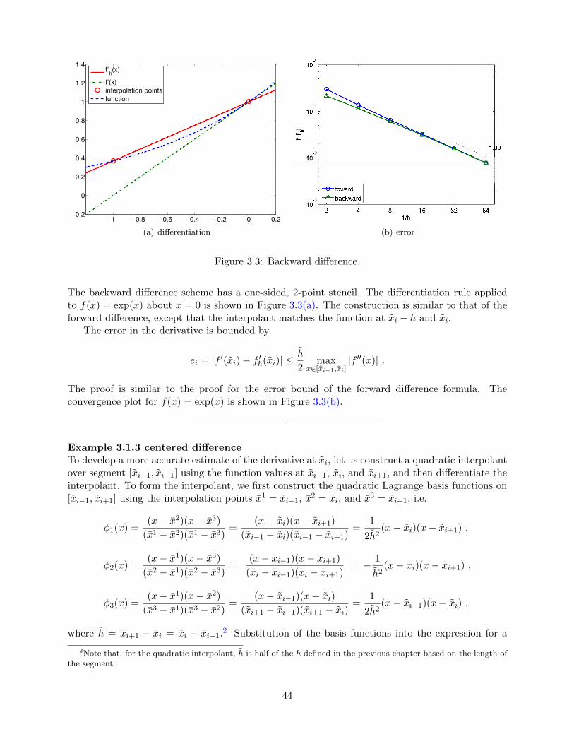
quadratic interpolant, Eq. (2.4), yields

(If)(x) = f(x1)φ1(x) + f(x2)φ2(x) + f(x3)φ3(x)

=1

2h2f(xi−1)(x− xi)(x− xi+1)− 1

h2f(xi)(x− xi−1)(x− xi+1)

+1

2h2f(xi+1)(x− xi−1)(x− xi) .

Differentiation of the interpolant yields

(If)′(x) =1

2h2f(xi−1)(2x− xi − xi+1)− 1

h2f(xi)(2x− xi−1 − xi+1) +

1

2h2f(xi+1)(2x− xi−1 − xi) .

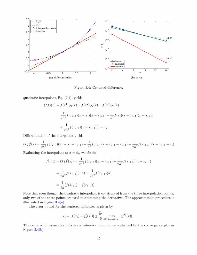
Evaluating the interpolant at x = xi, we obtain

f ′h(xi) = (If)′(xi) =1

2h2f(xi−1)(xi − xi+1) +

1

2h2f(xi+1)(xi − xi−1)

=1

2h2f(xi−1)(−h) +

1

2h2f(xi+1)(h)

=1

2h(f(xi+1)− f(xi−1)) .

Note that even though the quadratic interpolant is constructed from the three interpolation points,only two of the three points are used in estimating the derivative. The approximation procedure isillustrated in Figure 3.4(a).

The error bound for the centered difference is given by

ei = |f(xi)− f ′h(xi)| ≤h2

6max

x∈[xi−1,xi+1]|f ′′′(x)| .

The centered difference formula is second-order accurate, as confirmed by the convergence plot inFigure 3.4(b).

45

Proof. The proof of the error bound follows from Taylor expansion. Recall, assuming f ′′′(x) isbounded in [xi−1, xi+1],

f(xi+1) = f(xi + h) = f(xi) + f ′(xi)h+1

2f ′′(xi)h

2 +1

6f ′′′(ξ+)h3 ,

f(xi−1) = f(xi − h) = f(xi)− f ′(xi)h+1

2f ′′(xi)h

2 − 1

6f ′′′(ξ−)h3 ,

for some ξ+ ∈ [xi, xi+1] and ξ− ∈ [xi−1, xi]. The centered difference formula gives

(If)′(xi) =1

2h(f(xi+1)− f(xi−1))

=1

2h

[(f(xi) + f ′(xi)h+

1

2f ′′(xi)h

2 +1

6f ′′′(ξ+)h3

)

−(f(xi)− f ′(xi)h+

1

2f ′′(xi)h

2 − 1

6f ′′′(ξ−)h3

)]

= f ′(xi) +1

12h2(f ′′′(ξ+)− f ′′′(ξ−)

).

The error in the derivative estimate is∣∣f ′(xi)− (If)′(xi)∣∣ =

∣∣∣∣ 1

12h2(f ′′′(ξ+)− f ′′′(ξ−)

)∣∣∣∣ =1

6h2 max

x∈[xi−1,xi+1]|f ′′′(x)| .

Using a higher-order interpolation scheme, we can develop higher-order accurate numericaldifferentiation rules. However, the numerical stencil extends with the approximation order, becausethe number of interpolation points increases with the interpolation order.

·We would also like to make some remarks about how noise affects the quality of numerical

differentiation. Let us consider approximating a derivative of f(x) = exp(x) at x = 0. However,assume that we do not have access to f itself, but rather a function f with some small noise addedto it. In particular, let us consider

g(x) = f(x) + ε sin(kx) ,

with ε = 0.04 and k = 1/ε. We can think of ε sin(kx) as noise added, for example, in a measuringprocess. Considering f(0) = 1, this is a relatively small noise in terms of amplitude.

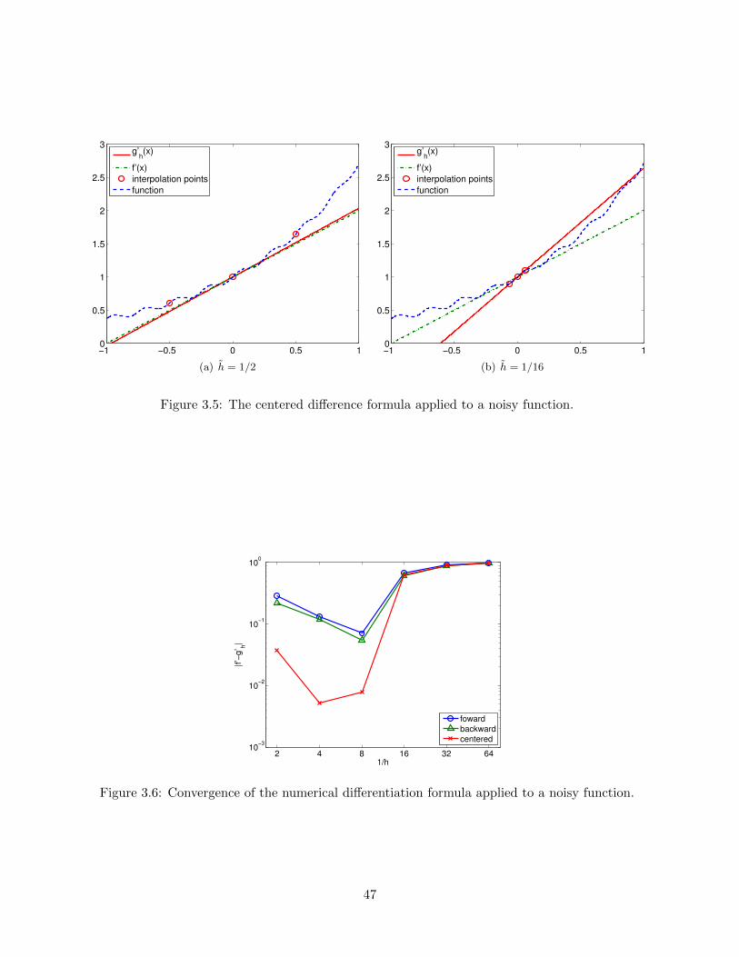
The result of applying the finite difference formulas to g in an attempt to approximate f ′(0)is shown in Figure 3.5. Comparing the approximations obtained for h = 1/2 and 1/16, we seethat the approximation in fact gets worse as h is refined. Figure 3.6 confirms that all numericaldifferentiation formulas considered in this section fail to converge. In fact, they all asymptoticallycommit O(1) error as h→ 0, even though the error decreases to less than 10−2 for a certain choiceof h.

46

−1 −0.5 0 0.5 10

0.5

1

1.5

2

2.5

3

g’h(x)

f’(x)

interpolation points

function

(a) h = 1/2

−1 −0.5 0 0.5 10

0.5

1

1.5

2

2.5

3

g’h(x)

f’(x)

interpolation points

function

(b) h = 1/16

Figure 3.5: The centered difference formula applied to a noisy function.

2 4 8 16 32 6410

−3

10−2

10−1

100

1/h

|f’−

g’ h

|

foward

backward

centered

Figure 3.6: Convergence of the numerical differentiation formula applied to a noisy function.

47

As essentially any data taken in real life is inherently noisy, we must be careful when differ-entiating the data. For example, let us say that our objective is to estimate the acceleration ofan object by differentiating a velocity measurement. Due to the presence of measurement noise,we in general cannot expect the quality of our acceleration estimate to improve as we improve thesampling rate and decreasing the discretization scale, h.

One strategy to effectively differentiate a noisy data is to first filter the noisy data. Filtering is atechnique to clean a signal by removing frequency content above a certain frequency3 For example,if a user is only interested in estimating the behavior of a signal below a certain frequency, allcontent above that threshold can be deemed noise. The cleaned data is essentially smooth withrespect to the scale of interest, and thus can be safely differentiated. Another alternative, discussedin Unit III, is to first fit a smooth function to many data points and then differentiate this smoothfit.

3.1.1 Second Derivatives

Following the same interpolation-based template, we can develop a numerical approximation tohigher-order derivatives. In general, to estimate the pth-derivative, we must use an interpolationrule based on pth- or higher-degree polynomial reconstruction. As an example, we demonstrate howto estimate the second derivative from a quadratic interpolation.

Example 3.1.4 second-order centered differenceWe can use the quadratic interpolant considered in the previous case to estimate the second deriva-tive of the function. Again, choosing x1 = xi−1, x2 = xi, x

3 = xi+1 as the interpolation points, thequadratic reconstruction is given by

(If)(x) = f(xi−1)φ1(x) + f(xi)φ2(x) + f(xi+1)φ3(x) ,

where the Lagrange basis function are given by

φ1(x) =(x− xi)(x− xi+1)

(xi−1 − xi)(xi−1 − xi+1),

φ2(x) =(x− xi−1)(x− xi+1)

(xi − xi−1)(xi − xi+1),

φ3(x) =(x− xi−1)(x− xi)

(xi+1 − xi−1)(xi+1 − xi).

Computing the second derivative of the quadratic interpolant can be proceeded as

(If)′′(x) = f(xi−1)φ′′1(x) + f(xi)φ′′2(x) + f(xi+1)φ′′3(x) .

In particular, note that once the second derivatives of the Lagrange basis are evaluated, we canexpress the second derivative of the interpolant as a sum of the functions evaluated at three points.

3Sometimes signals below a certain frequency is filtered to eliminate the bias.

48

The derivatives of the Lagrange basis are given by

φ′′1(x) =2

(xi−1 − xi)(xi−1 − xi+1)=

2

(−h)(−2h)=

1

h2,

φ′′2(x) =2

(xi − xi−1)(xi − xi+1)=

2

(h)(−h)= − 2

h2,

φ′′3(x) =2

(xi+1 − xi−1)(xi+1 − xi)=

2

(2h)(h)=

1

h2.

Substitution of the derivatives to the second derivative of the quadratic interpolant yields

(If)′′(xi) = f(xi−1)

(1

h2

)+ f(xi)

(−2

h2

)+ f(xi+1)

(1

h2

)=

1

h2

(f(xi−1)− 2f(xi) + f(xi+1)

).

The error in the second-derivative approximation is bounded by

ei ≡ |f ′′(xi)− (If)′′(xi)| ≤h2

12max

x∈[xi−1,xi+1]|f (4)(x)| .

Thus, the scheme is second-order accurate.

Proof. The proof of the error bound again follows from Taylor expansion. Recall, assuming f (4)(x)is bounded in [xi−1, xi+1],

f(xi+1) = f(xi + h) = f(xi) + f ′(xi)h+1

2f ′′(xi)h

2 +1

6f ′′′(xi)h

3 +1

24f (4)(ξ+)h4 ,

f(xi−1) = f(xi − h) = f(xi)− f ′(xi)h+1

2f ′′(xi)h

2 − 1

6f ′′′(xi)h

3 +1

24f (4)(ξ−)h4 .

The second derivative estimation gives

(If)′′(xi) =1

h2

[(f(xi) + f ′(xi)h+

1

2f ′′(xi)h

2 +1

6f ′′′(xi)h

3 +1

24f (4)(ξ+)h4

)

− 2f(xi)

+

(f(xi)− f ′(xi)h+

1

2f ′′(xi)h

2 − 1

6f ′′′(xi)h

3 +1

24f (4)(ξ−)h4

)]

= f ′′(xi) +1

24h2(f (4)(ξ+) + f (4)(ξ−)

).

The error in the second derivative is

|f ′′(xi)− (If)′′(xi)| =∣∣∣∣ 1

24h2(f (4)(ξ+) + f (4)(ξ−)

)∣∣∣∣ ≤ 1

12h2 max

x∈[xi−1,xi+1]|f (4)(x)| .

49

Let us demonstrate that the second-order derivative formula works for constant, linear, andquadratic function. First, we consider f(x) = c. Clearly, the second derivative is f ′′(x) = 0. Usingthe approximation formula, we obtain

(If)′′(xi) =1

h2

(f(xi−1)− 2f(xi) + f(xi+1)

)=

1

h2(c− 2c+ c) = 0 .

Thus, the approximation provides the exact second derivative for the constant function. This isnot surprising, as the error is bounded by the fourth derivative of f , and the fourth derivative ofthe constant function is zero.

Second, we consider f(x) = bx+c. The second derivative is again f ′′(x) = 0. The approximationformula gives

(If)′′(xi) =1

h2

(f(xi−1)− 2f(xi) + f(xi+1)

)=

1

h2[(bxi−1 + c)− 2(bxi + c) + (bxi+1 + c)]

=1

h2[(b(xi − h) + c)− 2(bxi + c) + (b(xi + h) + c)] = 0 .

Thus, the approximation also works correctly for a linear function.Finally, let us consider f(x) = ax2 + bx+ c. The second derivative for this case is f ′′(x) = 2a.

The approximation formula gives

(If)′′(xi) =1

h2[(ax2

i−1 + bxi−1 + c)− 2(ax2i + bxi + c) + (ax2

i+1 + bxi+1 + c)]

=1

h2[(a(xi − h)2 + b(xi − h) + c)− 2(ax2

i + bxi + c) + (a(xi + h)2 + b(xi + h) + c)]

=1

h2

[a(x2

i − 2hxi + h2)− 2ax2i + a(x2

i + 2hxi + h2)]

=1

h2

[2ah2

]= 2a .

Thus, the formula also yields the exact derivative for the quadratic function.

·The numerical differentiation rules covered in this section form the basis for the finite difference

method — a framework for numerically approximating the solution to differential equations. Inthe framework, the infinite-dimensional solution on a domain is approximated by a finite numberof nodal values on a discretization of the domain. This allows us to approximate the solution tocomplex differential equations — particularly partial differential equations — that do not haveclosed form solutions. We will study in detail these numerical methods for differential equations inUnit IV, and we will revisit the differential rules covered in this section at the time.

We briefly note another application of our finite difference formulas: they may be used (say)to approximately evaluate our (say) interpolation error bounds to provide an a posteriori estimatefor the error.

3.2 Differentiation of Bivariate Functions

Let us briefly consider differentiation of bivariate functions. For simplicity, we restrict ourselves toestimation of the first derivative, i.e., the gradient.

50

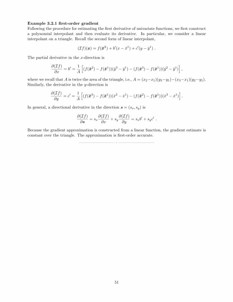
Example 3.2.1 first-order gradientFollowing the procedure for estimating the first derivative of univariate functions, we first constructa polynomial interpolant and then evaluate its derivative. In particular, we consider a linearinterpolant on a triangle. Recall the second form of linear interpolant,

(If)(x) = f(x1) + b′(x− x1) + c′(y − y1) .

The partial derivative in the x-direction is

∂(If)

∂x= b′ =

1

A

[(f(x2)− f(x1))(y3 − y1)− (f(x3)− f(x1))(y2 − y1)

],

where we recall that A is twice the area of the triangle, i.e., A = (x2−x1)(y3−y1)−(x3−x1)(y2−y1).Similarly, the derivative in the y-direction is

∂(If)

∂y= c′ =

1

A

[(f(x3)− f(x1))(x2 − x1)− (f(x2)− f(x1))(x3 − x1)

].

In general, a directional derivative in the direction s = (sx, sy) is

∂(If)

∂s= sx

∂(If)

∂x+ sy

∂(If)

∂y= sxb

′ + syc′ .

Because the gradient approximation is constructed from a linear function, the gradient estimate isconstant over the triangle. The approximation is first-order accurate.

·

51

52

Chapter 4

Elements of a Program and MatlabBasics

4.1 Computer Architecture and Computer Programming

4.1.1 Virtual Processor

It is convenient when programming a computer to have a mental model of the underlying architec-ture: the components or “units,” functions, and interconnections which ultimately implement theprogram. It is not important that the mental model directly correspond to the actual hardware ofany real computer. But it is important that the mental model lead to the right decisions as regardshow to write correct and efficient programs.

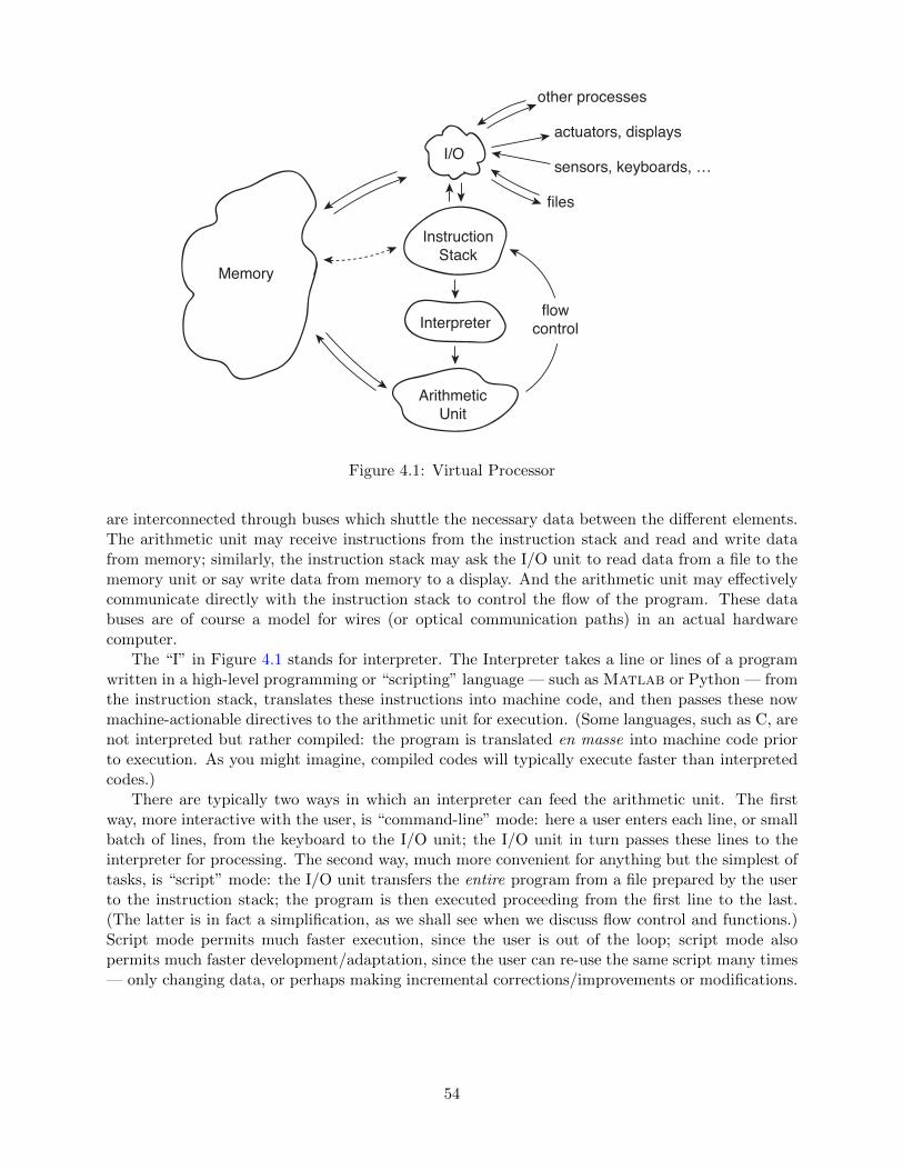
We show in Figure 4.1 the architecture for a “virtual computer.” There are many ways inwhich we can extend or refine our model to more accurately represent either particular processes orparticular computers of interest: we might break down each unit into smaller units — for example, amemory hierarchy; we might consider additional, special-purpose, units — for example for graphicsand visualization; and we might replicate our virtual computer many times to represent (a systemof) many interacting processes. We emphasize that if you put a screwdriver to computer case, youwould not find a one-to-one mapping from our virtual entities to corresponding hardware elements.But you might come close.

We now describe the different elements. On the far left we indicate the memory. This memoryis often hierarchical: faster and more expensive memory in a “cache”; slower and much more ex-tensive “RAM.” (Note also there will be archival memory outside the processor accessed throughI/O functions, as described shortly.) Next there is the arithmetic unit which performs the various“basic” operations on data — for example, assignment, addition, multiplication, and comparison.(The adjective “arithmetic” for this unit is overly restrictive, but since in this course we are primar-ily focused on numerical methods the key operations are indeed arithmetic.) We also identify the“instruction stack” which contains the instructions necessary to implement the desired program.And finally there is the I/O (Input/Output) unit which controls communication between our pro-cessor and external devices and other processes; the latter may take the form of files on archivalmedia (such as disks), keyboards and other user input devices, sensors and actuators (say, on arobot), and displays.

We note that all the components — memory, arithmetic unit, instruction stack, I/O unit —

53

DRAFT V2.1 © The Authors. License: Creative Commons BY-NC-SA 3.0.

Memory

I/O

InstructionStack

Interpreter

ArithmeticUnit

flowcontrol

other processes

actuators, displays

sensors, keyboards, …

files

Figure 4.1: Virtual Processor

are interconnected through buses which shuttle the necessary data between the different elements.The arithmetic unit may receive instructions from the instruction stack and read and write datafrom memory; similarly, the instruction stack may ask the I/O unit to read data from a file to thememory unit or say write data from memory to a display. And the arithmetic unit may effectivelycommunicate directly with the instruction stack to control the flow of the program. These databuses are of course a model for wires (or optical communication paths) in an actual hardwarecomputer.

The “I” in Figure 4.1 stands for interpreter. The Interpreter takes a line or lines of a programwritten in a high-level programming or “scripting” language — such as Matlab or Python — fromthe instruction stack, translates these instructions into machine code, and then passes these nowmachine-actionable directives to the arithmetic unit for execution. (Some languages, such as C, arenot interpreted but rather compiled: the program is translated en masse into machine code priorto execution. As you might imagine, compiled codes will typically execute faster than interpretedcodes.)

There are typically two ways in which an interpreter can feed the arithmetic unit. The firstway, more interactive with the user, is “command-line” mode: here a user enters each line, or smallbatch of lines, from the keyboard to the I/O unit; the I/O unit in turn passes these lines to theinterpreter for processing. The second way, much more convenient for anything but the simplest oftasks, is “script” mode: the I/O unit transfers the entire program from a file prepared by the userto the instruction stack; the program is then executed proceeding from the first line to the last.(The latter is in fact a simplification, as we shall see when we discuss flow control and functions.)Script mode permits much faster execution, since the user is out of the loop; script mode alsopermits much faster development/adaptation, since the user can re-use the same script many times— only changing data, or perhaps making incremental corrections/improvements or modifications.

54

4.1.2 The Matlab Environment

In Matlab the user interface is the command window. The command window provides the prompt>> to let the user know that Matlab is ready to accept inputs. The user can either directly enterlines of Matlab code after the >> prompt in command-line mode; alternatively, in script mode,the user can enter >> myscript.m to execute the entire program myscript.m. The suffix .m indicatesthat the file contains a Matlab program; files with the .m suffix are affectionately known as “mfiles.” (We will later encounter Matlab data files, which take the .mat suffix.) Note that mosteasily we run Matlab programs and subprograms (such as functions, discussed shortly) from thefolder which contains these programs; however we can also set “paths” which Matlab will searchto find (say) myscript.m.

Matlab in fact provides an entire environment of which the command window is just one(albeit the most important) part. In addition to the command window, there is a “current folder”window which displays the contents of the current directory — typically .m files and .mat files, butperhaps also other “non-Matlab ” (say, document) files — and provides tools for navigation withinthe file system of the computer. The Matlab environment also includes an editor — invoked bythe “Edit” pull-down menu — which permits the user to create and modify .m files. Matlab alsoprovides several forms of “manual”: doc invokes an extensive documentation facility window andsearch capability; and, even more useful, within the command window >>help keyword will bringup a short description of keyword (which typically but not always will be a Matlab “built–in”function). Similar environments, more or less graphical, exist for other (interpreted) programminglanguages such as Python.

We note that in actual practice we execute programs within programs within programs. We bootthe system to start the Operating System program; we launch Matlab from within in OperatingSystem to enter the Matlab environment; and then within the Matlab environment we run ascript to execute our particular (numerical) program. It is the latter on which we have focusedin our description above, though the other layers of the hierarchy are much better known to the“general computer user.” It is of course a major and complicated task to orchestrate these differentprograms at different levels both as regards process control and also memory and file management.We will illustrate how this is done at a much smaller scale when we discuss functions within theparticular Matlab context.

4.2 Data Types (and Classes)

All data in the computer is stored as 0’s and 1’s — binary digits. This is most convenient asbinary operations are very efficiently effected in terms of the necessary nonlinear circuit elements.The basic unit of memory is the “word-length” of the machine — the number of binary digits, or“bits,” which are used to represent data. Most machines these days are based on 32-bit or 64-bitwords (which are 4 Bytes and 8 Bytes, respectively); in some cases particular data types might berepresented by two words (or more).

But obviously we will need to interpret these 0’s and 1’s in different ways: in some cases the0’s and 1’s might represent machines codes (instructions) which tell the arithmetic unit what toexecute; in other cases, the 0’s and 1’s might represent data on which the the instructions willoperate (the “operands”). Furthermore, there are many different type of data: any piece of data isdefined not just by the 0’s and 1’s that make up the word, but also by the “data type” which tellsthe computer how to interpret and operate upon the data. As regards the latter, we note that thesame set of 0’s and 1’s can mean something very different — and be operated on in very differentways — depending on the data type associated with these 0’s and 1’s.

55

There are several important types within Matlab (and homologous types within other pro-gramming languages). There are logical variables which are either 0 or 1 which correspond respec-tively to (and in fact the data may be entered as) false or true . There is integer data — asigned whole number. There is character data, in which the 0’s and 1’s encode particular characterssuch as letters in the alphabet or numerals — the famous ASCII code and recent extensions. Andparticularly important for us, there are floating point numbers, which in Matlab are 64 bits andare called (for largely historical reasons) simply double. Representation of floating point numbers(FPNs) by a 64 bits is probably less obvious than representation of a whole number, and hencewe will discuss representation of FPNs, and also floating point operations, in a separate section.Matlab also supports a complex floating point type. These types are “atomic” in that they arepart of the core Matlab scripting language.

In some programming languages the user is required upon creation of a variable to specify thedata type. (We define variables in the next section — for now, think of a variable as the nameof a particular piece of data.) Each variable must be an instance of one of the available (in ourcase, Matlab ) data types. Matlab is much less picky than other programming languages — ablessing and a curse — and typically if no type is specified Matlab will simply assume a (double)floating point number, which is hence the “default.”

It is, however, possible to specify that any particular variable is logical, with the logical

function, an integer, with the (say) int32 command, a character, with the char command (ormore simply with quotes), and a floating point number, with the double command. We can alsodetermine what type of data a particular variable is with the islogical, isinteger, ischar, andisfloat functions.

We already above and will frequently below refer to functions. We do not fully define functionsuntil a later chapter, in which we learn how to create our own functions. For now, think of a functionas a program which takes some (zero, one, two, or many) input arguments and yields some output;we provide illustrations in the next section. All of the functions we describe in the precedingparagraph are “built-in” functions that are part of the core Matlab scripting language; we shallexercise these functions in the next section once we are armed with the assignment operation.(In fact, false (and true) are also built-in Matlab functions: false takes no arguments andreturns a logical zero.) Note the Matlab “core” is quite large compared to other languages suchas Python, in which most functions must be explicitly brought in as modules. There are, however,official Matlab extensions to the core, known as “toolkits.” In actual practice, functions can yieldmany outputs, not just a single output; we discuss this extension in a later chapter.

We note that often we might perform operations on data of different types. In that case wemight effect “conversion” before proceeding with the operation, or we might let the programminglanguage automatically perform “coercion” — conversion to a common data type based on rulesof precedence. For example, in Matlab , if we attempt to add an integer and a floating pointnumber, Matlab will (effectively) first convert the integer variable to a floating point variable.(Note that even when we invoke the various round, fix, floor, and ceil Matlab functions toround a floating point number (the input) to an integer ( the output), the output is of data typedouble.) In most cases Matlab makes reasonable choices, though on occasion more direct controlis warranted.

Finally we note that there is another term used to describe the proper specification and inter-pretation of given data: “class.” Typically data type is part of the language whereas data classesare created by the user. And typically data type would refer to a word or maybe two words whereasclass would refer to a compound type of many words (each of which might be specified as a differentdata type). Class also has a special significance in object-oriented programming: a class definesnot just a compound data type (an instance of which is known as an “object”), but also functionsor “methods” on members of this class. Matlab supports object-oriented programming both ex-

56

plicitly and implicitly, however we will only briefly touch on object-oriented programming in thiscourse, and primarily for purposes of interpretation of various operators.

This section is rather abstract simply because we do not yet know how to create data andhence we can not demonstrate any of the concepts. As already indicated, we shall illustrate thenotion of data types, the matlab functions used to define variables of a particular data type, andthe functions used to query variables as to their data type, once we learn how to create variables— in the next section.

4.3 Variables and Assignment

The assignment statement is the most basic operation. We proceed by example (using the command-line input mode):

>> pi_approx = 3.14159

pi_approx =

3.1416

>>

where we enter the material after the prompt >> and Matlab responds as indicated in the linesbelow the prompt line. In general, Matlab will display the result of an operation in the commandwindow unless we put a semi-colon at the end of the instruction.

It is important to understand what this statement actually does. The variable pi_approx is aname to which Matlab will associate a unique address — a location in memory; hence the variablepi_approx is in fact an address (a name), not a value. The assignment statement puts the value3.14159 at the address pi_approx. Again, pi_approx is the address, or reference, or pointer, orbox, which contains the value. If we change the value

>>pi_approx = 3.14

pi_approx =

3.14

>>

we are simply replacing the earlier value 3.14159 at address pi_approx with the new value 3.14 atthe same address pi_approx.

In the above assignment statement the = is an operator (and an operator which is part of the coreMatlab functionality). An operator is a function which takes one or two arguments and producesan output; operators, given the few operands, can be conveniently represented as a symbol. In thenext few sections we will introduce a number of useful operators. In terms of an operator, = looksto the right for the value and then places this value in the address indicated to the left.

In our assignment for pi_approx the way in which we have entered the number ensures thatpi_approx is of type floating point double. But we can be more explicit as in

57

>> pi_approx = double(3.14159)

pi_approx =

3.1416

>> floatcheck = isfloat(pi_approx)

floatcheck =

1

>>

which confirms that the double function indeed produces a variable of data type double.We emphasize that both double and isfloat are functions. The general syntax for a function

is simple: the input or inputs are included in parentheses following the function name, and theoutput (later, many outputs) — the evaluation of the function — is assigned to the variable to theleft of the =. For example, isfloat takes as input a variable — here the input is pi_approx — andreturns as output a logical variable which indicates whether the input is a floating point number —here the output is a 1 (true), since pi_approx is indeed a floating point number (or more precisely,an instance of the floating point double data type).

It is worth dissecting the above example a bit further. In fact, the statement

>> floatcheck = isfloat(pi_approx)

floatcheck = 1

>>

is a very simple example of a very powerful capability — composition. In particular, in this casewhen = looks to the right it finds not a value but a function, isfloat; the function isfloat isthen evaluated and the output of isfloat ( a logical 1) is then taken as the (right) input to the =

(assignment) operator; the = then looks to the left, floatcheck, to know where in memory to writethis value (a logical 1) (or to create a memory location with the “name” floatcheck, as needed).

We invite the reader to input a logical with logical and check that the result is logical withislogical, and an integer with int32 and check that the result is integer with isinteger. We willdiscuss characters and strings later in a separate section. Most often we will use the double datatype, which is the Matlab default and requires no special attention — we just enter the numberas 3.14159. We will also make extensive use of the logical data type.

4.4 The Workspace and Saving/Loading Data

In the previous section, we created variables such as pi_approx and floatcheck. Where do thesevariables go? These variables — and all variables we, or the programs we launch from the commandwindow, create — go to what is known as the “workspace.” In some sense, the workspace is thepart of the memory in Figure 4.1 (interpreted as the Matlab environment) which has already beenallocated. In order to see all the variables in our workspace we can do >> who. Note that >> who

58

does not evaluate the variables and hence does not provide the values; rather, it provides a list ofall the variable names to which we have assigned data. (To determine the value of a particularvariable we would simply type >>variable.) Note that whos is the same as who but with additionalinformation about size and data type (or “class”) of each variable.

If we wish to delete all the variables in the workspace, and start anew, we would do clear. (Thisof course only affects the Matlab variables you have created, with no effect on the file system —such as the .m files you might have created.) Alternatively, you might wish to just delete certainvariables, say variable 1 and variable 2 , in which case we would do >> clear variable 1 variable 2 .For smaller programs memory management is not an issue, but for larger programs it is importantto clear or more generally allocate and de-allocate memory carefully.

It is often the case that we wish to save the results of our calculations for future use — ratherthan re-compute. This is done very simply in Matlab : to save variables variable 1 and variable 2to a data file save_for_later.mat we do save save_for_later variable 1 variable 2 . To reloadthis data we simply do load save_for_later which will include the contents of save_for_later,in our case variable 1 and variable 2 , in the current workspace — that is, in addition to the currentcontents of your workspace. Note the .mat file is a Matlab specific data file which is the mostconvenient within Matlab , but there are also many other (and more universal) formats in whichdata can be saved.

4.5 Arithmetic Operations

We now turn to arithmetic operations, typically performed in Matlab on floating point numbers(though the operators also work on integers and indeed logicals through coercion, as discussedabove).

As already indicated, an operator is a function, syntactically represented by a symbol, whichtakes one or two input arguments, or parameters, or operands, and returns a result. The arithmeticoperators are ^ (exponentiation), / (division), * (multiplication), + (addition), and - (subtraction).These operations do the obvious thing, applied either to data or variables.

We consider addition: for data,

>> 2 + 3

ans =

5

or for variables

>> x = 2; y = 3;

>> x + y

ans =

5

>>

59

(Note the semi-colons suppress display of x and y; if we wish to confirm the value, we need only do(say) >> x without a semi-colon to evaluate x.) In more detail, the + operator takes the two valuesto the left and right and outputs as the answer (ans) the sum. The other arithmetic operators ^,/, *, and -, perform in a similar obvious fashion.

We note that in the above x + y is an expression — here a single function, but more generallya composition of many operations — which is evaluated to yield the result ans. Note when we doan evaluation of an expression expr , Matlab “finishes” the statement for us as ans = expr — inother words, Matlab assigns the result of the evaluation to a variable ans. We can in fact use thisvariable ans subsequently, but this is highly frowned upon since, as you can imagine, it is quiteeasy for the generic ans to be changed in unanticipated or unnoticed ways.

Rather, if we wish to subsequently use the result of an evaluation, we should explicitly assignthe output to a variable, say z: we need only do

>> z = x + y

z = 5

>>

which is a composition of the addition ( +) operator with the assignment ( =) operator: we evaluatethe expression (or operation, or function) x + y and then assign the result of this evaluation to avariable z.

We repeatedly above refer to the addition “function.” In fact, for most operators there is an“output = function name (inputs)” syntax which is equivalent to the operator syntax. For instance,we may compute the sum of x and y as plus(x,y). Obviously the operator form is much easierand more readable, however the plus contains the actual code which implements addition andfurthermore provides a mechanism by which to change what we mean by addition for different datatypes (and in the object-oriented context, different classes). We do not recommend that you changethe definition of plus for double data types — but in fact, it is quite easy to do, and could provean effective form of industrial numerical sabotage.

It is instructive to consider the statement

>> z = z + 1

z = 6

>>

which in fact serves quite often in iterative procedures (typically for z an integer, even if representedin Matlab by a double). What does this statement do? First Matlab evaluates the expressionz + 1 to obtain the value 6; then operator = assigns this value 6 to the address (variable) z.Although mathematically z = z + 1 appears nonsensical, it is important to remember that inz = z + 1 the = is the assignment operator and not an equal sign. (Of course, Matlab contributesto the confusion in very next line, z = 6, by using the = sign in the convention mathematical senseof equality.)

Up to this point we have composed operators for which we did not need to worry about theorder in which we performed the operations. For example, 3 + 4 + 5 can be evaluated either as(3 + 4) + 5 (i.e., 3 + 4 first, then + 5). (In fact, this is not quite true in finite precision, as wediscuss in the next section.) On the other hand, 3*2^4 gives quite different results if we perform

60

either the * first or the ^ first. Matlab thus provides rules of precedence for the order in whichoperators are evaluated: first the items in parentheses, from the inside out; then ^; then / and *;then + and -. The mnemonic is PEDMAS (not very mnemonic, in fact). If the rules of precedencedo not not dictate a unique order then Matlab operates from left to right.

The easiest way to avoid misinterpretation of your intentions is to liberally use parentheses,and for readability to always include ample spaces within and between your parentheses. Theevaluation of 3*2^4 gives us opportunity to introduce the notion of a bug. If you intended (3*2)^4

but simply wrote 3*2^4 Matlab would do something different from your intentions. This is notMatlab ’s fault, but your fault. There are many kinds of bugs: a statement may in fact notcorrespond to valid Matlab syntax and the statement will not even be interpreted; a statementmay correspond to valid Matlab syntax but may do something other than intended by the user— as in our 3*2^4 example; the statement may do what the users intends but in fact to achievethe desired end the user’s intentions are not correct — this occurs quite frequently in the contextof numerical computation.

4.6 Floating Point Numbers (FPNs): Representation and Opera-tions

4.6.1 FPN Truncation and Representation

Floating point numbers represent a challenge both in how we represent these numbers and in howwe perform arithmetic operations on these numbers. To begin, we express a number x in base 2 as

x = σ1

∞∑k=0

bk2−k

× 2σ2E ,

in which the bk are binary numbers — 0 or 1, E is an integer, and σ1 and σ2 are signs — ±1. Weassume that we have normalized the expansion such that b0 = 1. (In fact, we may express x in saybase 10 rather than base 2; this in turn will lead to a different floating point format.)

In some cases, we may only require a finite sum — a sum with a finite number of nonzero terms— to represent x. For example, x = 2 may be expressed by the single non-zero term b0 = 1 (andE = +1). However more generally a finite number of non-zero bk will not suffice — even 1/10leads to a repeating binary fraction. We thus must truncate the series to develop the floating pointnumber (FPN) approximation of x:

xFPN = σ1

K∑k=0

b′k2−k

× 2σ2E′.

Here b′k = bk, 1 ≤ k ≤ K — we perform truncation of our series — and E′ is the minimum of Eand Emax — we truncate the range of the exponent.

We now represent or encode xFPN in terms of (a finite number of) 0’s and 1’s. Towards thisend we assign one bit each to the signs σ1 and σ2; we assign p = K bits for the binary numbers b′k,1 ≤ k ≤ K, to represent the mantissa (or significand); we assign pE bits to represent the exponentE (and hence Emax = 2pE). (Our choice of base 2 makes the encoding of our approximation in 0’sand 1’s particularly simple.) In the 64-bit IEEE 754 binary double (now called binary64) floatingpoint format, p = 52 and pE = 10 (corresponding to Emax = 310 such that in total — including thesign bits — we require 2+52+10 = 64 bits. (The storage scheme actually implemented in practiceis slightly different: we need not store the leading unity bit and hence we effectively realize p = 53;the exponent sign σ2 is in fact represented as a shift.)

61

There are two primary sources or types of error in the approximation of x by xFPN: the firstis FPN truncation of the mantissa to p bits; the second is the FPN truncation of the exponent topE bits. The former, FPN mantissa truncation, is generally rather benign given the rather largevalue of p. However, in some cases, FPN mantissa truncation errors can be seriously amplified byarithmetic operations. The latter, FPN exponent truncation, takes the form of either overflow —exponents larger than 310, represented in Matlab as plus or minus Inf — which is typically anindication of ill-posedness, or underflow — exponents smaller than −310, represented in Matlabas 0 — which is typically less of a concern.

We note that the word “precision” is typically reserved to indicate the number of bits or dig-its with which a floating point number is approximated on any particular hardware (and IEEEformat); typically we focus on the mantissa. For example, 64-bit precision, or “double-precision,”corresponds to 52 (or 53) binary digits of precision — roughly 16 decimal digits of precision —in the mantissa. Precision can also be characterized in term of “machine precision” or “machineepsilon” which is essentially the (relative) magnitude of the FPN truncation error in the worst case:we can find machine epsilon from the Matlab built-in function eps, as we will illustrate below.We will define machine epsilon more precisely, and later construct a code to find an approximationto machine epsilon, once we have understood floating point arithmetic.

Oftentimes we will analyze a numerical scheme in hypothetical “infinite-precision” arithmeticin order to understand the errors due to numerical approximation and solution in the absence offinite-precision FPN truncation effects. But we must always bear in mind that in finite precisionarithmetic additional errors will be incurred due to the amplification of FPN truncation errors byvarious arithmetic operations. We shortly discuss the latter in particular to identify the kinds ofoperations which we should, if possible, avoid.

Finally, we remark that there are many ways in which we may choose to display a number sayin the command window. How we display the number will not affect how the number is stored inmemory or how it is approximated in various operations. The reader can do >> help format tounderstand the different ways to control the length of the mantissa and the form of the exponent indisplayed floating point numbers. (Confusingly, format in the context of how we display a numbercarries a different meaning from format in the context of (IEEE) FPN protocol.)

4.6.2 Arithmetic Operations

We shall focus on addition since in fact this particular (simple) operation is the cause of mostdifficulties. We shall consider two numbers x1 and x2 which we wish to add: the first numberhas mantissa m1 and exponent E1 and the second number has mantissa m2 and exponent E2. Wepresume that E1 > E2 (if not, we simply re-define “first” and “second”).

First, we divide the first mantissa by 2E1−E2 to obtain m′2 = m22−(E1−E2): in this form, x1 nowhas mantissa m′2 and exponent E1 . (Note this division corresponds to a shift of the mantissa: toobtain m′2 we shift m1 by E1−E2 places to the right — and pad with leading zeros.) At this stagewe have lost no precision. However, in actual practice we can only retain the first p bits of m′2(since we only have p bits available for a mantissa): we denote by m′′1 the truncation of m1 to fitwithin our p-bit restriction. Finally, we perform our FPN sum z = x1 +x2: z has mantissa m1 +m′′2and exponent E1. (Our procedure here is a simplification of the actual procedure — but we retainmost of the key features.)

We can immediately see the difficulty: as we shift m2 to the right we are losing E1 −E2 bits ofprecision. If the two exponents E1 and E2 are very different, we could lost all the significant digitsin x2. Armed with FPN we can in fact develop a simple definition of machine epsilon: the smallestepsilon such that 1 + epsilon = 1, where of course by + we now mean finite precision FPNaddition. Later we will take advantage of this definition to write a short program which computes

62

machine epsilon; for our purposes here, we shall simply use the Matlab built-in function eps.It is clear that finite-precision and infinite-precision arithmetic are different and will yield dif-

ferent results — the difference is commonly referred to as “round-off” error. Indeed, finite-precisionarthmetic does not even honor all the usual (e.g., commutative, associative) rules. We consider theexample (recall that in Matlab operations are performed from left to right in the absence of anyprecedence rules):

>> mach_eps = eps

mach_eps =

2.2204e-16

>> (mach_eps/2 + 1 + mach_eps/2 - 1)/mach_eps

ans =

0

>> (mach_eps/2 + mach_eps/2 + 1 - 1)/mach_eps

ans =

1

>>

Clearly, in infinite precision arithmetic both expressions should evaluate to unity. However, in finiteprecision the order matters: in the first expression by definition mach_eps/2 + 1 evaluates to 1; inthe second expression, mach_eps/2 + mach_eps/2 adds two numbers of identical exponent — noloss in precision — which are then large enough (just!) to survive addition to 1. This anomaly isa “bug” but can also be a feature: we can sometimes order our operations to reduce the effect ofround-off errors.

But there are situations which are rather difficult to salvage. In the following example weapproximate the derivative of sin(x) by a forward first-order difference with increment dx which isincreasingly small:

>> cos(pi/4)

ans =

0.707106781186548

>> dx = .01;

>> deriv_dx = (sin(pi/4 + dx) - sin(pi/4))/dx

deriv_dx =

0.703559491689210

63

>> dx = 1e-8;

>> deriv_dx = (sin(pi/4 + dx) - sin(pi/4))/dx

deriv_dx =

0.707106784236800

>> dx = 1e-20;

>> deriv_dx = (sin(pi/4 + dx) - sin(pi/4))/dx

deriv_dx =

0

>>

We observe that what Newton intended — and the error bound we presented in Chapter 3 — isindeed honored: as dx tends to zero the finite difference (slope) approaches the derivative (cos(π/4)).But not quite: as dx falls below machine precision, the numerator can no longer see the difference,and we obtain an O(1) error — precisely in the limit in which we should see a more and moreaccurate answer. (As the reader can no doubt guess, pi, sin, and cos are all Matlab built-infunctions.)

This is in fact very typical behavior. In order to make numerical errors small we must takesmaller increments or many degrees-of-freedom, however if we go “too far” then finite-precisioneffects unfortunately “kick in.” This trade-off could in fact be debilitating if machine precisionwere not sufficiently small, and indeed in the early days of computing with only a relatively fewbits to represent FPNs it was a struggle to balance numerical accuracy with finite precision round-off effects. These days, with the luxury of 64-bit precision, round-off errors are somewhat less of aconcern. However, there are situations in which round-off effects can become important.

In particular, we note that the problem is our derivative example is not just the numerator butalso the dx in the denominator. As a general rule, we wish to avoid — where possible — divisionby small numbers, which tends to amplify the effects of finite-precision truncation. (This relatesto stability , which is an important theme which we will encounter in many, often related, guisesin subsequent chapters.) We will see that even in much more sophisticated examples — solutionof large linear systems — “avoid division by small numbers” remains an important guideline andoften a feature (by construction) of good algorithms. The problem of course is aggravated whenwe must perform many operations as opposed to just a few operations.

We have focused our attention on addition since, as indicated, this operation is often the prox-imal cause of the round-off difficulties. Other operations are performed in the “obvious” way. Forexample, to multiply two numbers, we multiply the mantissas and add the exponents and thenre-adjust to conform to the necessary representation. Division and exponentiation follow similarrecipes. Obviously underflow and overflow can be undesired byproducts but these are typicallyeasier to avoid and not “fundamental.”

64

4.7 Relational and Logical Operations

4.7.1 Relational Operations

A relational operator performs some kind of comparison between two variables (typically floatingpoint double) and then returns a logical variable to indicate the outcome of the comparison. Therelational operators are equal, ==; not equal, ~=; less than, <; greater than, >; less than or equal, <=;greater than or equal, >=. Note that the equal operator, ==, is now interpreted in the mathematicalsense of = (vs. the Matlab assignment operator = which of course serves a different function).

As an example, we consider

>> x = 4.6; y = 4.7;

>> isless = x < y

isless =

1

>>

Here Matlab first evaluates the expression x < y — which, since x is less than y, is a truestatement, and hence returns a logical 1 — and then assigns this value of 1 to the (logical) variableisless. (As we know, floating point numbers are truncated in finite precision arithmetic; since the< operates on the truncated form, of course the comparison is only good to machine precision.)

We can of course consider composition. Typically, composition of relational operations is bylogical operations, as we now discuss. (In fact, we can apply usual arithmetic to logical variables,which are converted to floating point for the purpose. This is often convenient, but must be usedwith some care.)

4.7.2 Logical Operations

It would be possible to hi-jack operations such as + to perform Boolean operations on logicalvariables, however Matlab prefers to reserve the usual arithmetic functions for these operatorsapplied to logical variables. Hence we introduce new operators.

The three key logical operators are AND, indicated as &, OR, indicated as |, and NOT, indicatedas ~. (There are also other options, such as the exclusive or, or XOR.) The AND and OR operatorstake as (the two) operands logical variables and the result is of course also a logical variable. TheNOT takes a single logical operand and the result is also a logical variable. As already indicated,these logical operators are often composed with relational operators.

The AND, OR, and NOT behave in the expected fashion. The statement L3 = L1 & L2 yieldsL3 = 1 (true) only if both L1 and L2 are both == 1 (true), otherwise L3 = 0. The statementL3 = L1 | L2 yields L3 = 1 if either L1 == 1 or L2 == 1, otherwise L3 = 0 (note that if bothL1 == 1 and L2 == 1, then L3 = 1); conversely, L3 = 0 only if both L1 == 0 and L2 == 0. Fi-nally, the NOT: L3 = ~L1 yields L3 = 1 if L1 == 0 and L3 = 0 if L1 == 1.

As an example, we consider the AND and NOT:

>> x = 4.6; y = 4.7;

>> u = 3.1; v = 3.2;

>> z = (x < y) & ~(u < v)

65

z =

0

>>

which of course yields the correct result. Note the Matlab precedence convention is to evaluaterelational operators before logical operators and hence our parentheses in the above are redundant— but better too many parentheses than too few. And another example,

>> x = 4.6; y = 4.7;

>> u = 3.1; v = 3.2;

>> z = (x < y) | ~(u < v)

z =

1

>>

now with the OR and NOT.Finally, we mention that Matlab provides “short-circuit” versions of AND and OR, the oper-

ators for which are given by && and ||, respectively. These short-circuit operators will not evaluatethe second operand (i.e., to the right) if the first operand (i.e., to the left) suffices to make the de-cision. For example, in our OR example above, since x < y, z = (x < y) || ~(u < v) will onlyevaluate (x < y). This can lead to efficiencies — if the second operand is much more expensiveand or ensure that a (second) operand is only evaluated when it exists and is well-defined.

Logical (and relational) operations play a key role in flow control — in controlling the flow (or“direction”) of the program based on the results generated by the program itself. In some sense itis these logical and relations operations and the enabled flow control which distinguishes a programexecuted by a computer from arithmetic performed on a calculator.

4.8 Flow Control

4.8.1 The if Statement

The if statement is very simple. The general syntax is given by

if logical expression 1BLOCK 1

elseif logical expression 2BLOCK 2

else

BLOCK 3end

which is interpreted by Matlab as follows:

66

if logical expression 1 evaluates to true, execute BLOCK 1 and go to end (and continue onwith the next line in the program);

if logical expression 1 evaluates to false, but logical expression 2 evaluates to true, executeBLOCK 2 and go to end (and continue);

if logical expression 1 is false and logical expression 2 is false, execute BLOCK 3 and goto end (and continue).

Note several variants are possible: we may include multiple elseif statements between theBLOCK 1 and else; and we may omit the else and BLOCK 3 statements.

In the event that in fact there are many cases there is another Matlab statement which is nodoubt preferable to the if statement: the switch statement. We do not discuss the switch state-ment here, but rather use this opportunity to recall the very helpful help function: >> help switch

will provide you with a quick (but sufficient) description of the syntax and functionality of theswitch statement.

4.8.2 The while Statement

The syntax of the while statement is

initialize var 1, var 2,. . .while relational or logical expression while (var 1, var 2,. . . )

BLOCK % new values assigned to var 1, var 2, ...

end

This statement is a loop which is controlled by the value of the logical variable which is the result ofevaluation of relational_or_logical_expression_while. What makes the statement powerfulis that relational_or_logical_expression_while may depend on var 1, var 2, . . . , the valuesof which are changed at each pass through the loop. In particular, the while is executed as follows:if relational or logical expression while (var 1, var 2, . . . ) is true, execute (the instruction linesin) BLOCK , otherwise go to end and continue with next line of program of which the while ispart; repeat. Note that var 1, var 2, . . . must be initialized prior to entering the while loop.

As an example, we consider

>> i = 0;

>> sum_of_integers = 0;

>> while i <= 3

sum_of_integers = sum_of_integers + i;

i = i + 1;

end

>> sum

sum_of_integers =

6

>>

67

Here, relational or logical expression while (var 1) is the simple expression i <= 3, where i playsthe role of var 1. In fact, this particular sum is more easily performed with a for statement, as wedescribe shortly. The true value of the while is when the relational or logical expression is a morecomplicated function of the variables which are changed by the BLOCK and in particular when wedo not know a priori how many iterations through the loop will be required.

For example, we create the script machine eps.m

% script to calculate machine epsilon

mach_eps = 1;

while (1 + mach_eps ~= 1)

mach_eps = mach_eps/2.;

end

mach_eps

in the editor. Note that as we start to construct slightly longer programs we will start to use scriptmode rather than command-line mode. The input is easier, as are debugging and modification, andof course re-use. In addition, the editor within Matlab recognizes various keywords and automat-ically formats statements for improved readability. Note also the comment line: any material on aline which follows a % will be ignored by the interpreter and serves only to educate the author anduser’s as to the intent of the program or particular lines of the program.

We then enter in the command window

>> machine_eps

mach_eps =

1.1102e-16

>>

which runs our script. Of course this code is just calculating for us machine precision, which agreeswith the Matlab eps to within the factor of two related to our stopping tolerance.

Finally, we note that you may include a break in a BLOCK statement

if (relational or logical expression break) break

which will directly go to the end statement of the while loop quite independent of whetherrelational_or_logical_expression_while (for the current values of var 1, var 2, . . . ) is true

or false. Purists often try to avoid break statements, but pragmatists tolerate the occasionalbreak statement. Too many break statements may be a symptom of poor program design or moregenerally passive-aggressive tendencies.

4.8.3 The for Statement

The syntax for the for statement is

for VARCOUNTER = LIM 1 : INCREMENT : LIM 2BLOCK % no reassignment of VARCOUNTER

end

68

Typically LIM 1, INCREMENT, LIM 2 would be integers (even if of data type double), howeverthere are also many instances in which these variables could be (mathematically) non-integer. Notealso that INCREMENT can be positive or negative, and that if INCREMENT is not specified thenMatlab chooses the default value INCREMENT = 1.

The execution of the for loop is simple: we execute BLOCK for VARCOUNTER = LIM 1 ; weupdate VARCOUNTER = VARCOUNTER + INCREMENT ; then, if VARCOUNTER <= LIM 2 ,repeat. As for a while statement, we can interrupt the usual flow of the for loop with a break

statement. Note that if LIM 1 + INCREMENT is less than LIM 2 then BLOCK will never beexecuted.

We repeat our earlier example:

>> sum_of_integers = 0;

>> for i = 1:3

sum_of_integers = sum_of_integers + 1;

end

>> sum_of_integers

sum_of_integers =

3

>>

There are many situations in numerical methods in which the for loop is the ideal construct. How-ever, it is also true that in Matlab there are a number of functions related to array manipulationthat, although implicitly built upon a for construction, are typically more efficient than an explicitfor loop. We introduce some of these functions in the next section.

Finally, we note that our for syntax here is not as general as provided for by Matlab .However, the more general syntax requires the notions of single-index or multi-index arrays, whichwe have not yet introduced. Following the treatment of arrays the reader should do >> help for

to understand the generalization: in effect, we can require VARCOUNTER to cycle through anyparticular set of scalars (defined in a single-index array) or VARCOUNTER itself may even be asingle-index array which cycles through a particular set of single-index arrays (defined in a double-index array).

69

70

Chapter 5

Matlab Arrays

5.1 Single-Index Floating Point Arrays

5.1.1 The Concept

It is often the case that we have an ordered set of, say n, “elements” of data which are somehowrelated. The index could represent directions in three space dimensions (k = 1, 2, 3 for x, y, z,respectively) — at which we store, in each array location, the corresponding coordinate of a point(an array of length 3); or the index could represent 15 different times — at which we store, ineach location, the time of the measurement, or perhaps the measurement itself (an array of length15). Note the index plays the role of independent variable and the array value plays the role ofdependent variable. In all these cases we will often wish to operate on all n “related elements” ina similar fashion. We would thus like a way to reference all the elements with a common name,and an easy way to reference different elements through this common name, in order to developsuccinct, readable, and efficient code for implementing common operations on all the elements. Inparticular, we would not want to write n lines of code each time we wished, say, to square each ofthe n elements.

A single-index array — in this section, a floating point single-index array — is the simplest“class” which achieves these objectives. We first introduce a variable name, array name, whichshall be associated to all n elements of the array. We then index this array name in order to accessany particular element of the array: in particular, array name(i) is the pointer to element i of thearray. We emphasize that, as in the scalar case, array name(i) is not the value of element i ofthe array but rather the location in memory at which we shall store the value of element i. Forexample, array name(2) = 3.14159 would assign the value 3.14159 to the second element of thearray. (We discuss more efficient assignment methods below.)

Conceptually, you may think of the array as stored at n contiguous locations in memory. Ele-ment 1 of the array is stored in array name(1), element 2 of the array is stored in array name(2),. . . , and element n of the array is stored in array name(n). In this (virtual) sense, it suffices to(say) pass to a function simply the variable array name — which you may view as the addressof the first element — as the addresses of all the other elements of the array can then be readilydeduced from array name. (In actual practice, there is also some header information associatedwith the array — for example, in our single-index case, the length n.) Since many common arrayoperations can be performed in Matlab with simple function calls — or user-defined function

71

DRAFT V2.1 © The Authors. License: Creative Commons BY-NC-SA 3.0.

calls — at a high-level we can often deal exclusively with array name without explicit reference toparticular indices. (Of course, under the hood. . . )

5.1.2 Assignment and Access

The most explicit way to create a single-index array is by hand: X = [1,3,4] creates a single-index array of length 3, with entries X(1) = 1, X(2) = 3, and X(3) = 4. To determine thelength of an array Matlab provides a function length. In our example

>> X = [1,3,4]

X =

1 3 4

>> X(1)

ans = 1

>> length(X)

ans =

3

>>

Note that this single-index array is a row single-index array. (We can also consider column single-index arrays, in which the commas above are replaced by semi-colons: X = [1;3;4]. We reservetreatment of rows and columns to our discussion of double-index arrays.)

The input process is facilitated by the colon operator. In particular, Z = [J:D:K] createsthe single-index array J, J+ D,...,J + m*D] for m = fix((K-J)/D), where fix is a Matlabfunction which rounds to the nearest integer towards zero. (Note that J:D:K is empty if D == 0,if D > 0 & J > K, or if D < 0 & J < K.) The default value of D is 1 and hence J:K is equivalentto J:1:K, as in the example

>> firstfive = [1:5]

firstfive =

1 2 3 4 5

>>

You will in fact recognize this colon construction from the for statement; and indeed the for

statement may take the form for VARCOUNTER = S where S is any single-index array; we willrevisit this construction of the for statement shortly.

We may assign an entire array,

72

>> Y = X

Y =

1 3 4

>>

or we may assign or re-assign a particular element as, say,

>> X(3) = 10;

>> X

X =

1 3 10

>>

which we see modifies X accordingly.Of course the point of an array is that we have a systematic numerical approach to indexing,

and we may thus easily assign values with a for statement. We present two approaches. In thefirst, we zero out to initialize:

>> Z = zeros(1,10);

>> for i = 1:length(Z)

Z(i) = i^2;

end

>> Z

Z =

1 4 9 16 25 36 49 64 81 100

>>

Note that zeros(1,n) is a Matlab function which provides a (row) single-index array of all zerosof length n. (Note the first argument of zeros indicates that we wish to form a row single-indexarray; zeros(n, 1) would create a column single-index array of all zeros. We will understandzeros better once we discuss multi-index arrays.) This approach, of initialization, is preferredwhenever possible: it permits Matlab to be more efficient in memory allocation and management.

In the second approach, we concatenate:

>> Z = [];

>> for i = 1:10

Z = [Z,i^2];

end

>> Z

73

Z =

1 4 9 16 25 36 49 64 81 100

>>

Here Z = [] defines an array but the array is initially empty: we do this because we can not“add to” (append to, or concatenate to) an array which does not exist. Note that the expression[Z, i^2] evaluates to an array in which the first length(Z) elements are the elements of Z and thelast element is i^2. Thus at each iteration the length of Z grows. The above is less efficient thanthe initialization approach, but very convenient in particular (for example, in a while statement)when we do not a priori know the number of elements in our (ultimate) array.

As our last point on assignment and access, we note that Matlab supports a very convenientform of indirect addressing. In particular, if we create a single-index array of integers indvec thenwe can extract from (say) Z just those elements with indices in indvec:

>> indvec = [1,3,5,9];

>> U = Z(indvec)

U =

1 9 25 81

>>

Note you may also apply indirect addressing on the left-hand side of the assignment statement, butsome care must be exercised as regards the “shape” (row vs. column) of the resulting single-indexarray.

Note that in all these shortcuts there is always an equivalent underlying program (which is moreor less how these shortcuts are implemented). For example, in the above, an array index argumenttells Matlab to execute, effectively:

>> U_too = zeros(1,length(indvec))

>> for inew = 1:length(indvec)

U_too(inew) = Z(indvec(inew));

end

>> U_too

U_too =

1 9 25 81

>>

But of course much better to encapsulate and re-use this feature within the Matlab syntax thanto re-write this little loop on each occasion.

74

5.1.3 (Dotted) Arithmetic Operations

It is one of the major advantages of programming languages that as we develop more convenient datastructures (or types, or classes), in particular with many elements, we may also suitably define ouroperations to deal directly with these new entities — as a whole, rather than explicitly manipulatingeach element. In this section we define for the case of single-index arrays the corresponding arrayarithmetic operators.

We first discuss element-by-element operations. In these operations, we consider two arrays ofthe same length and we apply the same arithmetic operation on each pair of elements which sharethe same index. We begin with addition/subtraction (and multiplication by a scalar):

>> P = [1, 4, 7]; Q = [2, -1, 1];

>> R = P + 3.0*Q

R =

7 1 10

>>

which is simply shorthand for the loop

>> for i = 1:length(P)

R_too(i) = P(i) + 3.0*Q(i);

end

>> R_too

R_too =

7 1 10

>>

The loop makes clear the interpretation of “element by element,” but obviously the one-line state-ment is much preferred.

Note 3.0 is not an array, it is scalar , which scales all elements of the array Q in our aboveexample. This simple scaling feature can be very convenient in defining arrays of grid points or datapoints (for example, in interpolation, differentiation, and integration). To wit, if we have an intervalof length L and wish to createN segments of length L/N , we need only do >> xpts = (L/N)*[0:N].Note that xpts is of length (in the sense of number of elements in the array) N+1 since include bothendpoints: xpts(1) = 0 and xpts(N+1) = L/N.

Finally, we note one additional shortcut: if q is a scalar, then element-by-element addition toour vector P will add q to each element of P. To wit,

>> q = 3;

>> P + q

ans =

75

4 7 10

>>

We might write the above more properly as

>> P + q*ones(1,length(P))

ans =

4 7 10

>>

but there is no need given Matlab ’s automatic expansion of q when encountered in array addition.Note ones(1,n) is a Matlab function which creates a (row) single-index array of length n withall elements set to unity.

To implement element-by-element multiplication, division, and exponentiation we do

>> PdotmultQ = P.*Q

PdotmultQ =

2 -4 7

>> PdotdivideQ = P./Q

PdotdivideQ =

0.5000 -4.0000 7.0000

>> PdotexpQ = P.^Q

PdotexpQ =

1.0000 0.2500 7.0000

>>

which is equivalent to

>> for i = 1:length(P)

PdotmultQ_too(i) = P(i)*Q(i);

PdotdivideQ_too(i) = P(i)/Q(i);

PdotexpQ_too(i) = P(i)^Q(i);

end

>> PdotmultQ_too

PdotmultQ_too =

76

2 -4 7

>> PdotdivideQ_too

PdotdivideQ_too =

0.5000 -4.0000 7.0000

>> PdotexpQ_too

PdotexpQ_too =

1.0000 0.2500 7.0000

>>

As for addition, if we replace one of our vectors by a scalar, Matlab will expand out with a “ones”vector.

Why do we need the “dot” before the *, /, and ^ operators — so-called “dotted” (or element-by-element) operators: dotted multiplication, dotted division, and dotted exponentiation? It turns outthat there are two types of entities which look very similar, respectively arrays and vectors (latermulti-index arrays and matrices): both are ordered sets of n floating point numbers. However, thearithmetic operations are defined very differently for these two entities, respectively element-by-element operations for arrays and linear algebraic operations (e.g., inner products) for vectors. Wecould easily define say * to perform element-by-element multiplication for objects which are definedas arrays, and to perform an inner product for objects defined as vectors. Unfortunately, althoughconceptually quite clean, this would be very cumbersome since often in one line we wish to treat aset of numbers as an array and in the next line we wish to treat the same set of numbers as a vector:there would be much conversion and bookkeeping. Hence Matlab prefers a kind of “superclass”of array-and-vector (and matrix) entities, and hence perforce some new syntax to indicate whetherwe wish to treat the array-and-vector as an array (with dotted element-by-element operators) or avector (with undotted linear algebra operators). Note that we do not require dotted + (or dotted-) since element-by-element addition and vector addition in fact are equivalent. So there.

We note that there are many arithmetic operations on arrays in addition to element-by-elementoperations, many of which are available as Matlab functions. For example, we can easily performthe sum of the first three integers (as we did earlier with a for loop) as

>> ints = [1:3];

>> sum(ints)

ans =

6

>> mean(ints)

ans =

77

2

>>

where sum performs the sum of all the elements in an array (here ints) and mean calculates thearithmetic mean of all the element in an array.

Finally, we note here that the many Matlab built-in mathematical functions — we have alreadyencountered sin and cos, but there are many many more — look for “math function” and “specialfunctions” in the doc — which also accept single-index (and in fact, double–index) arguments. Forexample,

>> xpts = (pi/4)*0.5*[0:2];

>> sin_values = sin(xpts)

sin_values =

0 0.3827 0.7071

>>

with a single call provides the values of sin for all elements of xpts.

5.1.4 Relational and Logical (Array) Operations

For relational and logical operations we do not have the complication of array/vector conflation andhence we need no dots. In effect, when we apply any of our scalar relational/ logical operations topairs of vectors of the same length, Matlab returns a vector (of the same length as the operands)which is the result of the scalar relational/logical operation element-by-element.

As an example,

>> x = [1.2, 3.3, 2.2]; y = [-0.1, 15.6, 2.0];

>> z_1 = (x < y)

z_1 =

0 1 0

>> z_2 = (x > y)

z_2 =

1 0 1

>> z_3 = z_1 | ~z_2

z_3 =

0 1 0

78

>>

Similar example can be constructed for all of our relational operators and logical operators. Notethat z_1, z_2 and z_3 are logical arrays: each element is an instance of the logical data type.

For completeness, we indicate the implementation of the above as a for loop:

>> for i = 1:length(x)

z_1_too(i) = (x(i) < y(i));

z_2_too(i) = (x(i) > y(i));

z_3_too(i) = z_1_too(i) | ~ z_2_too(i) ;

end

>> z_1_too

z_1_too =

0 1 0

>> z_2_too

z_2_too =

1 0 1

>> z_3_too

z_3_too =

0 1 0

>>

which is indeed equivalent, but tedious.

5.1.5 “Data” Operations

There are also a number of operations which albeit numerical are focused as much on the indicesas the data — and hence we include these under the heading “data” operations.

A number of Matlab functions are available to reorder the elements or to identify distinguishedelements: sort, min, and max are perhaps the most useful in this regard. We illustrate just one ofthese functions, min:

>> T = [4.5, -2.2, 6.3, 4.4];

>> [minimum, minimizer] = min(T)

minimum =

-2.2000

79

minimizer =

2

>> minimum_too = min(T)

minimum_too =

-2.2000

>>

which yields the obvious result. This is our first example of a function with two outputs: minimumis the minimum of the array, and minimizer is the index of the minimizing element. Note also thatif we just wish to obtain the first output we can abbreviate the call.

Perhaps one of the most useful array data functions is the find function. Given a logical vectorL, find(L) will return a vector which contains (in increasing order) the indices of all the elementsof L which are nonzero (and are hence unity, since L is a logical array). (In fact, find can also beapplied to a double array, but one must be careful about round-off effects.) As an example:

>> L = logical([0,1,1,0,0,1]);

>> islogical(L)

ans =

1

>> ind_of_nonzero = find(L)

ind_of_nonzero =

2 3 6

>>

where we have also illustrated the construction of a logical vector. Note that the find functioneffectively implements the for loop

>> ind_of_nonzero_too = [];

>> for i = 1:length(L)

if( L(i) ~= 0 )

ind_of_nonzero_too = [ind_of_nonzero_too,i];

end

end

>> ind_of_nonzero_too

ind_of_nonzero_too =

2 3 6

80

>>

which demonstrates also an application of concatenation.The function find is very useful in the context of comparisons. For example, we may wish to

extract just those values of vector greater than some threshold:

>> H = [0.2, 1.4, 6.7, -3.4, 4.2];

>> log_H_thresh = (H > 1.2)

log_H_thresh =

0 1 1 0 1

>> inds_H_thresh = find(log_H_thresh)

inds_H_thresh =

2 3 5

>> H(inds_H_thresh)

ans =

1.4000 6.7000 4.2000

>>

We can of course replace H > 1.2 in the above with any more complicated composition of relationaland logical operators.

We could of course combine this as

>> H ( find ( H > 1.2 ) )

ans =

1.4000 6.7000 4.2000

>>

In fact, Matlab accepts a further abbreviation as

>> H ( H > 1.2 )

ans =

1.4000 6.7000 4.2000

>>

81

in which a find is automatically applied to a logical index vector. Apparently this somewhatsyntactically sloppy approach is in fact the most efficient.

We take this opportunity to revisit the for statement. We initially introduced the for statementof the form for VARCOUNTER = LIM_1:INC:LIM_2 and later noted that the for statement may takea more general form for VARCOUNTER = S where S is any single-index array. We now present anexample of this general form of the for statement. Our objective is to find a number of entries in a(row) single-index array that are positive. As before, we can write the for loop based on an indexas

>> scalars = [1,-3,1,2,-5];

>> num_pos = 0;

>> for i = 1:length(scalars)

if (scalars(i) > 0)

num_pos = num_pos + 1;

end

end

>> num_pos

num_pos =

3

>>

which gives the expected result. Alternatively, we may use our set of scalars directly as the argumentto the for loop. That is

>> scalars = [1,-3,1,2,-5];

>> num_pos = 0;

>> for sca = scalars

if (sca > 0)

num_pos = num_pos + 1;

end

end

>> num_pos

num_pos =

3

>>

which also gives the correct result. In this second form, within the for loop, the loop argumentsca is first set to the first element of scalars, 1, sca is then set to the second element of scalars,-3, and so on.

We may interpret the (restrictive) form of the for statement for VARCOUNTER = LIM_1:INC

:LIM_2 within this general form: LIM_1:INC:LIM_2 first yields an single-index array [LIM_1,

LIM_1+INC, ..., LIM_2] (assuming LIM_2 = LIM_1 + m*INC for some integer m); then the for

loop successively assigns an element of the array to VARCOUNTER. (We note that the argument of

82

the for loop must be a row single-index array, not a column single-index array. We revisit thispoint in our discussion of the for statement using double-index arrays.)

5.2 Characters and Character Single-Index Arrays (Strings)

Our focus is on numerical methods and hence we will not have too much demand for characterand string processing. However, it is good to know the basics, and there are instances — typicallyrelated to more sophisticated applications of software system management, “codes that write codes”(or less dramatically, codes some lines of which can be modified from case to case), and alsosymbolic manipulation — in which character concepts can play an important role. Note thatcharacter manipulation and symbolic manipulation are very different: the former does not attributeany mathematical significance to characters; the latter is built upon the former but now addsmathematical rules of engagement. We consider here only character manipulation.

A character variable (an instance of the character data type), say c, must represent a letterof numeral. As always, c ultimately must be stored (ultimately) by 0’s and 1’s. We thus need —as part of the data type definition — an encoding of different characters in terms of 0’s and 1’s.The most common such encoding, the original ASCII code, is a mapping from 8-bit words (binarynumbers) to the set of letters in the alphabet, numerals, punctuation marks, as well as some specialor control characters. (There are now many “extended” ASCII codes which include symbols fromlanguages other than English.)

We can create and assign a character variable as

>> c = '3'

c =

3

>> c_ascii = int8(c)

c_ascii =

51

>> c_too = char(c_ascii)

c_too =

3

>>

In the first statment, we enter the single-character data with quotes — which tells Matlab that3 is to be interpreted as a character and not a number. We can then obtain the ASCII codefor the number 3 — which happens to be 51. We can then recreate the character variable c bydirectly appealing to the ASCII code with the char command. Obviously, quotes are easier thanmemorizing the ASCII code.

A “string” is simply a single-index array of character elements. We can input a string most

83

easily with the quote feature:

>> pi_approx_str = '3.1416'

pi_approx_str =

3.1416

>> pi_approx_str(2)

ans =

.

>> pi_approx_str + 1

ans =

52 47 50 53 50 55

>>

We emphasize that pi_approx_str is not of type double and if we attempt to (say) add 1 topi_approx_str we get (effectively) nonsense: Matlab adds 1 to each element of the ASCII-translation of the our string according to the rules of single–index array addition.

We can readily concatenate strings, for example:

>> leader = 'The value is '

leader =

The value is

>> printstatement = [leader,pi_approx_str,' .']

printstatement =

The value is 3.1416 .

>>

However, this is of limited use since typically we would know an approximation to π not as a stringbut as double.

Fortunately, there are some simple conversion functions available in Matlab (and other pro-gramming languages as well). The Matlab function num2str will take a floating point numberand convert it to the corresponding string of characters; conversely, str2num will take a string (pre-sumably of ASCII codes for numerals) and convert it to the corresponding floating point (double)data type. So for example,

84

>> pi_approx_double = str2num(pi_approx_str)

pi_approx_double =

3.1416

>> pi_approx_str_too = num2str(pi_approx_double)

pi_approx_str_too =

3.1416

>>

This can then be used to create a print statement based on a floating point value (e.g., obtainedas part of our numerical calculations):

>> printstatement_too = [leader,num2str(pi_approx_double),' .']

printstatement_too =

The value is 3.1416 .

>>

In actual practice there are higher level printing functions (such as fprintf and sprintf) inMatlab built on the concepts described here. However, the above rather low-level constructs canalso serve, for example in developing a title for a figure which must change as (say) the time towhich the plot corresponds changes.

5.3 Double-Index Arrays

5.3.1 Concept

Double-index arrays (and more generally, multi-index arrays), are extremely important in theimplementation of numerical methods. However, conceptually, they are quite similar to single-index arrays, and inasmuch this section can be rather short: we just consider the “differentialinnovation.” In fact, as we will see shortly, a double-index array really is a single-index array asfar as internal representation in memory or “address space”: the two indices are just a convenientway to access a single-index array.

Reference by two indices (or three indices,. . . ) can be convenient for a variety of reasons: ina 10× 10 structured rectilinear mesh, the two indices might represent the location of a point in a“Cartesian” grid — at which we store, in each array location, say the value of the temperature field(a 10× 10 array); in an unstructured three-dimensional mesh (or a Monte Carlo random sample),the first index might represent the label/order of a point within a sample of say length 1000, and thesecond index might represent the spatial coordinate direction (e.g., 1, 2, 3 for the x, y, z directions)— at which we store, in the array locations, the coordinate of the point (a 1000 × 3 array); andmost notably, the two indices might represent the rows and columns of an m×n matrix — at whichwe store the matrix values (an m × n array). (We discuss matrices in depth later.) Recall that

85

the indices play the role of the independent variable and the array values the role of the dependentvariable.

For a double-index array, just as for a single-index array, we first introduce a variable name,array name, but now this double-index array is associated to m × n elements: we may think ofa double-index arrays as m rows by n columns, as we shall visualize shortly. We then index thisarray name to access any particular element of the array: in particular, array name(i,j) is thepointer to element i, j of the array. As always, the pointer is the location in memory at which westore the value of the array.

In fact, even this double-index array is stored at contiguous locations in memory. (It is inthis sense that a double-index array is internally equivalent to a single-index array; we shall takeadvantage of this equivalence later.) Matlab stores a double-index array as “first address fastest”:array name(1,1),...,array name(m,1),array name(1,2),...,array name(m,2),...,array name(m,n). As for the single-index case, it suffices to to pass to a function simply thevariable array name — the address of the first element — as the addresses of all other elements canthen be readily deduced (in practice, thanks to appropriate header information). And of course,as for a single-index array, we will endeavor to similarly define operations on the entire array, asrepresented by array name, rather than treat each index separately.

A note on nomenclature: we can also think of single-index and double-index arrays as “one-dimensional” and “two-dimensional” arrays. However, we will reserve “dimension” for the linearalgebra sense: a vector with n entries is a member of n-dimensional space. Hence the linear algebra“dimension” is analogous to the Matlab length. (And just to make sure this paragraph, inattempting to avoid confusion, is sufficiently confusing: to avoid confusion of Matlab length

with the linear algebra “length” of a vector we shall refer to the latter as the “norm” of the vector.We return to this point in Unit 3.)

5.3.2 Assignment and Access

We start with a simple example and then explain the syntax.

>> A = [1,2,3;4,5,6]

A =

1 2 3

4 5 6

>> size_of_A = size(A)

size_of_A =

2 3

>> A(2,2)

ans =

5

>>

86

We see that a comma separates elements within a row, and a semicolon separates different rows.The size function returns a single-index array of length 2: the first element is the number of rows— the limit for the first index — and the second element is the number of columns — the limit forthe second index. Finally, we see that we can access individual elements of A as (say) A(2,2). Ofcourse our interpretation as rows and columns is just an artifice — but a very useful artifice whichwe invoke on many many occasions — for visualization and interpretation.

Our row single-index array is special case of double-index array:

>> X = [1,3,4]

X =

1 3 4

>> size(X)

ans =

1 3

>> X(1,3)

ans =

4

>>

And we can now systematically introduce a column single-index array as

>> X_col = [1;3;4]

X_col =

1

3

4

>> size(X_col)

ans =

3 1

>> X_col(3,1)

ans =

4

87

>>

Note in this case each row is of length 1 so we require no comma delimiters. Note operations inMatlab require arrays of similar size, so always make sure that pairs of single-index array operandsare both row arrays or both column arrays. This is best ensured by initialization of the array withzeros and consistent assignment.

The transpose operation is very convenient: it “flips” the two indices. Hence

>> A_transp = A'

A_transp =

1 4

2 5

3 6

>> X'

ans =

1

3

4

>> size(X')

ans =

3 1

>>

Rows become columns and columns become rows. (In fact, the transpose operator is a special caseof a more general Matlab function reshape which allows us to “resize” an array.)

As always, the reader should mentally note the more expanded code which effects any particularoperation to make sure the operation is well understood: in this case

>> for i = 1:size(A,1)

for j = 1:size(A,2)

A_transp_too(j,i) = A(i,j);

end

end

>> A_transp_too

A_transp_too =

1 4

2 5

88

3 6

>>

Note that size(A,1) and size(A,2) conveniently return the first element and second element ofsize(A).

As for single-index arrays, we can directly assign an entire double-index array: B = A creates anew array B identical to A in terms of size as well as values; we may also assign or re-assign anyparticular element of the array as selected by the index — for example, B(1,1) = 0. Oftentimeswe can create the desired array as an assignment plus modification of an existing array.

We may also create an array with a “double” for loop:

>> m = 2;n = 3;

>> A = zeros(m,n);

>> for i = 1:size(A,1)

for j = 1:size(A,2)

A_too(i,j) = j + (i-1)*size(A,2);

end

end

>> A_too

A_too =

1 2 3

4 5 6

>>

Note initialization of multi-index arrays is particularly important since these arrays tend to belarger and memory management even more of an issue.

However, concatenation also works for multi-index arrays and can be very effective.

>> R1 = [1,2,3]; R2 = [4,5,6];

>> C1 = [1;4]; C2 = [2;5]; C3 = [3;6];

>> A_too_too = [R1; R2]

A_too_too =

1 2 3

4 5 6

>> A_too_too_too = [C1,C2,C3]

A_too_too_too =

1 2 3

4 5 6

>> A_four_times = [A_too, A_too; A_too, A_too]

89

A_four_times =

1 2 3 1 2 3

4 5 6 4 5 6

1 2 3 1 2 3

4 5 6 4 5 6

>> A_four_times_also = [[A_too;A_too],[A_too;A_too]]

A_four_times_also =

1 2 3 1 2 3

4 5 6 4 5 6

1 2 3 1 2 3

4 5 6 4 5 6

>> A_four_times_expand_by_one = [A_four_times,[C1;C2]; [R1,R2],0]

A_four_times_expand_by_one =

1 2 3 1 2 3 1

4 5 6 4 5 6 4

1 2 3 1 2 3 2

4 5 6 4 5 6 5

1 2 3 4 5 6 0

>>

The general procedures for concatenation are somewhat difficult to succinctly describe — we mustalways combine entities that “match” in the direction in which we concatenate — but the casesabove include most instances relevant in numerical methods.

We can also do indirect addressing for double-index arrays, as we illustrate on our arrayA_four_times. In particular, let ind1vec and ind2vec be single-index arrays given by (say)

>> ind1vec = [2,3]

ind1vec =

2 3

>> ind2vec = [2:4]

ind2vec =

2 3 4

>>

90

Then

>> extracted = A_four_times(ind1vec,ind2vec)

extracted =

5 6 4

2 3 1

>>

which in fact is implemented as

>> for i = 1:length(ind1vec)

for j = 1:length(ind2vec)

extracted_too(i,j) = A_four_times(ind1vec(i),ind2vec(j));

end

end

>> extracted_too

extracted_too =

5 6 4

2 3 1

>>

This can be very useful for extracting rows and columns, as we now describe.In particular, to extract say row 1 or column 2 of A, we need only do

>> R1_too = A(1,1:size(A,2))

R1_too =

1 2 3

>> C2_too = A(1:size(A,1),2)

C2_too =

2

5

>>

In fact, Matlab conveniently provides a function end which, when it appears in the place of kth

index (k = 1 or k = 2), evaluates to (say for our array A) size(A,k). We then can write moresuccinctly

91

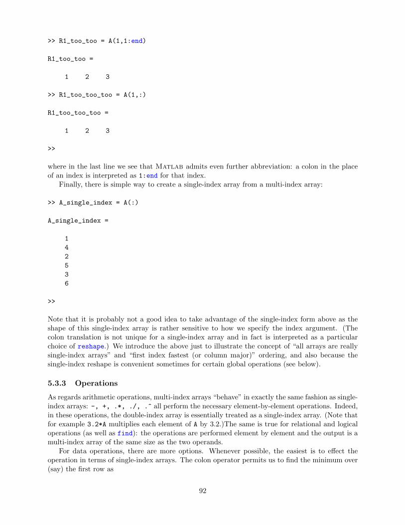
>> R1_too_too = A(1,1:end)

R1_too_too =

1 2 3

>> R1_too_too_too = A(1,:)

R1_too_too_too =

1 2 3

>>

where in the last line we see that Matlab admits even further abbreviation: a colon in the placeof an index is interpreted as 1:end for that index.

Finally, there is simple way to create a single-index array from a multi-index array:

>> A_single_index = A(:)

A_single_index =

1

4

2

5

3

6

>>

Note that it is probably not a good idea to take advantage of the single-index form above as theshape of this single-index array is rather sensitive to how we specify the index argument. (Thecolon translation is not unique for a single-index array and in fact is interpreted as a particularchoice of reshape.) We introduce the above just to illustrate the concept of “all arrays are reallysingle-index arrays” and “first index fastest (or column major)” ordering, and also because thesingle-index reshape is convenient sometimes for certain global operations (see below).

5.3.3 Operations

As regards arithmetic operations, multi-index arrays “behave” in exactly the same fashion as single-index arrays: -, +, .*, ./, .^ all perform the necessary element-by-element operations. Indeed,in these operations, the double-index array is essentially treated as a single-index array. (Note thatfor example 3.2*A multiplies each element of A by 3.2.)The same is true for relational and logicaloperations (as well as find): the operations are performed element by element and the output is amulti-index array of the same size as the two operands.

For data operations, there are more options. Whenever possible, the easiest is to effect theoperation in terms of single-index arrays. The colon operator permits us to find the minimum over(say) the first row as

92

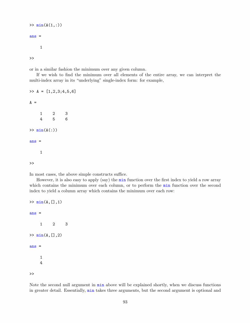
>> min(A(1,:))

ans =

1

>>

or in a similar fashion the minimum over any given column.If we wish to find the minimum over all elements of the entire array, we can interpret the

multi-index array in its “underlying” single-index form: for example,

>> A = [1,2,3;4,5,6]

A =

1 2 3

4 5 6

>> min(A(:))

ans =

1

>>

In most cases, the above simple constructs suffice.However, it is also easy to apply (say) the min function over the first index to yield a row array

which contains the minimum over each column, or to perform the min function over the secondindex to yield a column array which contains the minimum over each row:

>> min(A,[],1)

ans =

1 2 3

>> min(A,[],2)

ans =

1

4

>>

Note the second null argument in min above will be explained shortly, when we discuss functionsin greater detail. Essentially, min takes three arguments, but the second argument is optional and

93

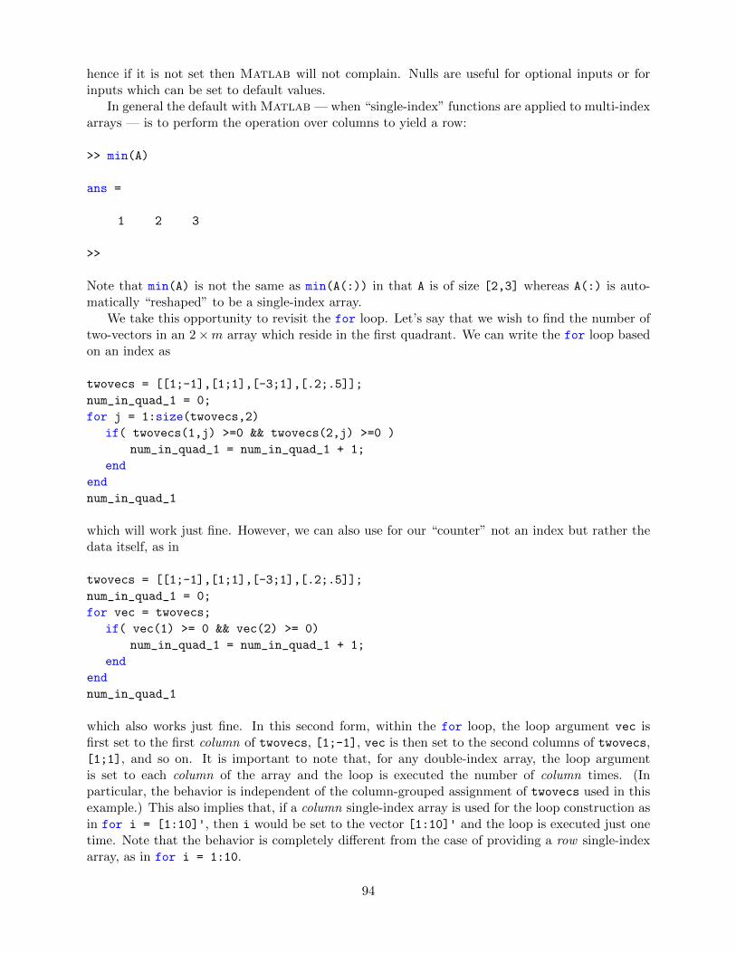
hence if it is not set then Matlab will not complain. Nulls are useful for optional inputs or forinputs which can be set to default values.

In general the default with Matlab — when “single-index” functions are applied to multi-indexarrays — is to perform the operation over columns to yield a row:

>> min(A)

ans =

1 2 3

>>

Note that min(A) is not the same as min(A(:)) in that A is of size [2,3] whereas A(:) is auto-matically “reshaped” to be a single-index array.

We take this opportunity to revisit the for loop. Let’s say that we wish to find the number oftwo-vectors in an 2×m array which reside in the first quadrant. We can write the for loop basedon an index as

twovecs = [[1;-1],[1;1],[-3;1],[.2;.5]];

num_in_quad_1 = 0;

for j = 1:size(twovecs,2)

if( twovecs(1,j) >=0 && twovecs(2,j) >=0 )

num_in_quad_1 = num_in_quad_1 + 1;

end

end

num_in_quad_1

which will work just fine. However, we can also use for our “counter” not an index but rather thedata itself, as in

twovecs = [[1;-1],[1;1],[-3;1],[.2;.5]];

num_in_quad_1 = 0;

for vec = twovecs;

if( vec(1) >= 0 && vec(2) >= 0)

num_in_quad_1 = num_in_quad_1 + 1;

end

end

num_in_quad_1

which also works just fine. In this second form, within the for loop, the loop argument vec isfirst set to the first column of twovecs, [1;-1], vec is then set to the second columns of twovecs,[1;1], and so on. It is important to note that, for any double-index array, the loop argumentis set to each column of the array and the loop is executed the number of column times. (Inparticular, the behavior is independent of the column-grouped assignment of twovecs used in thisexample.) This also implies that, if a column single-index array is used for the loop construction asin for i = [1:10]', then i would be set to the vector [1:10]' and the loop is executed just onetime. Note that the behavior is completely different from the case of providing a row single-indexarray, as in for i = 1:10.

94

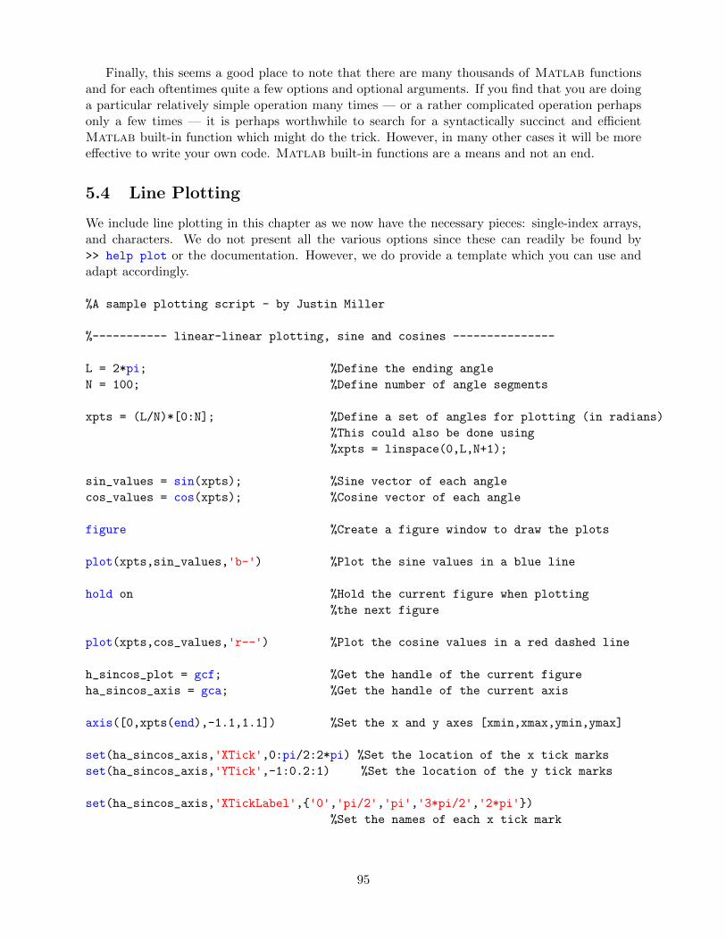
Finally, this seems a good place to note that there are many thousands of Matlab functionsand for each oftentimes quite a few options and optional arguments. If you find that you are doinga particular relatively simple operation many times — or a rather complicated operation perhapsonly a few times — it is perhaps worthwhile to search for a syntactically succinct and efficientMatlab built-in function which might do the trick. However, in many other cases it will be moreeffective to write your own code. Matlab built-in functions are a means and not an end.

5.4 Line Plotting

We include line plotting in this chapter as we now have the necessary pieces: single-index arrays,and characters. We do not present all the various options since these can readily be found by>> help plot or the documentation. However, we do provide a template which you can use andadapt accordingly.

%A sample plotting script - by Justin Miller

%----------- linear-linear plotting, sine and cosines ---------------

L = 2*pi; %Define the ending angle

N = 100; %Define number of angle segments

xpts = (L/N)*[0:N]; %Define a set of angles for plotting (in radians)

%This could also be done using

%xpts = linspace(0,L,N+1);

sin_values = sin(xpts); %Sine vector of each angle

cos_values = cos(xpts); %Cosine vector of each angle

figure %Create a figure window to draw the plots

plot(xpts,sin_values,'b-') %Plot the sine values in a blue line

hold on %Hold the current figure when plotting

%the next figure

plot(xpts,cos_values,'r--') %Plot the cosine values in a red dashed line

h_sincos_plot = gcf; %Get the handle of the current figure

ha_sincos_axis = gca; %Get the handle of the current axis

axis([0,xpts(end),-1.1,1.1]) %Set the x and y axes [xmin,xmax,ymin,ymax]

set(ha_sincos_axis,'XTick',0:pi/2:2*pi) %Set the location of the x tick marks

set(ha_sincos_axis,'YTick',-1:0.2:1) %Set the location of the y tick marks

set(ha_sincos_axis,'XTickLabel',{'0','pi/2','pi','3*pi/2','2*pi'})%Set the names of each x tick mark

95

xlabel('Angle (radians)') %Give a label name to the x axis

ylabel('Trigonomic output') %Give a label name to the y axis

title(['Plot of sin and cos from x = ',num2str(xpts(1)), ...

' to x = ',num2str(xpts(end))])%Give the figure a title

legend('sin','cos','location','best') %Provide a legend and tell matlab to place

%it in the best location

saveas(h_sincos_plot,'sin_cos.fig') %Take the figure specified by handle

%"h_sincos_plot" and save it

%as "sin_cos.fig" in the working directory

%----------- log-linear plotting, exponential ---------------

clear all

L = 5;

N = 100;

x = (L/N)*[0:N];

y = 2*exp(x);

figure

semilogy(x,y,'b-') %Create a plot where only the y axis is in log scale

%semilogx would plot only the x axis in log scale

xlabel('x')ylabel('y')

title(['Log-Linear plot of y = 2*exp(x) from x = ',num2str(x(1)), ...

' to x = ',num2str(x(end))])

saveas(gcf,'exp.fig')

%----------- log-log plotting, polynomials ---------------

clear all

L = 10^2;

N = 100;

x= (L/N)*[0:N];

y = 2*(x.^3);

figure

96

loglog(x,y,'b-') %Create a plot where both axes are in log scale

xlabel('x')ylabel('y')

title(['Log-Log plot of y = 2x^3 from x = ',num2str(x(1)), ...

' to x = ',num2str(x(end))])

saveas(gcf,'poly.fig')

Matlab also has extensive “3-D” plotting capabilities.

97

98

Chapter 6

Functions in Matlab

6.1 The Advantage: Encapsulation and Re-Use

As you know, a mathematical function is a “rule” which given some inputs (or arguments), returnsan output or outputs. A Matlab function (or a function in any programming language), is verysimilar: the function, given some inputs/arguments, returns an output or outputs. There are twomain reasons that functions are so important and useful as a programming construct: re-use andencapsulation. First, re-use: if we perform a particular set of operations — for example, calculationof sin(x) for given x — we prefer not to re-write this same code over and over again. Rather, wewrite it once and then use it over and over again, with enormous savings. Second, encapsulation: auser can take advantage of the function, and the “function” it performs — from inputs to outputs —without knowing how this function has been implemented or what is “inside” the code; from anotherperspective, what happens inside the function does not affect the user’s higher level objectives —the output is the entire “effect” (we discuss this further below).

We have already taken extensive advantage of both re-use and encapsulation: we have usedmany Matlab built-in functions in all of our examples above; and we have used these functionsnot only without knowing “what is inside” but in fact without even knowing how a function isdefined syntactically. In actual practice, it would not be good to proceed in quite such a trustingfashion.

6.2 Always Test a Function

Functions have serious implications as regards the correctness of results and the control of errors.From the positive side, the fact that the program is re-used many times, and developed onceintentionally for re-use, means that typically most bugs will have been identified and fixed. Fromthe negative side, encapsulation means that the user typically will not know what is inside, andhence can not personally vouch for correctness. The latter is, fortunately, quite easy to address ina reasonable if not rigorous fashion: confronted with any new function, it is alway worthwhile toconsider several test cases — for which you know the answer — to confirm correct behavior; themore authoritative the source, the more the function has been used, the simpler the task, perhapsthe less tests required. But remember that you are not just testing the code, you are also testingyour understanding of the inputs and outputs.

99

DRAFT V2.1 © The Authors. License: Creative Commons BY-NC-SA 3.0.

Note that is often difficult to find a test case in which we know the answer. In particular inthe numerical context there is an artifice by which to side-step this issue. In particular, it is oftenpossible to posit the answer and then easily determine the question (which yields this answer).For example, if we wish to test a code which finds the roots of a fourth-order polynomial, for anyparticular fourth-order polynomial it is not easy to deduce the correct answer (or we would notneed the code in the first place). However, it is easy to posit the four roots — the answer — andmultiply out to obtain the polynomial with these roots — the question. We then test the code bygoing backwards (in fact forwards), and verifying that the question leads to the answer. Note sucha test does not confirm that the code works in all cases; in fact, we have only confirmed one case.The numerical approach (or even the logic of the code) could thus be flawed in certain or even manyinstances. However, we have confirmed that we are using the code correctly, that we understandwhat in principle should happen, and that in at least one (or several) nontrivial cases that whatshould happen does indeed happen. You should always test a new function in this fashion.

We emphasize that our discussion here applies both to the many Matlab “built-in” functions— functions bundled with the Matlab core — and any third-party of user-defined function. Alsoin the remainder of this chapter many of the details are relevant both to built-in and user functions— for example, how to call a multi-output, multi-input function; however some details, such ashow to create a function, are obviously only important for user-defined functions.

6.3 What Happens in a Function Stays in a Function

When we launch a script (or a function) from the command window we may view this programas the “main” program (to use a somewhat archaic term). The (command-window) workspace ofthis main program is the set of variables of which the main program is aware (and which havebeen assigned at some point during the execution). When this main program calls a function, sayfunction name, we can view the process as the creation of a second virtual processor, as shownin Figure 6.1 2. In particular, it is critical to note that the two workspaces — the variablesassigned by the main program and by function name — are distinct: the main program is unawareof the variables in workspace function name and function name is unaware of the variables inworkspace command-window. The only connection between these two virtual processes are theinputs and outputs: function name receives the inputs from the main program, and the mainprogram receives the outputs from function name; note the direction of the arrows — inputs are notaffected by function name. Furthermore, workspace function name will disappear when executionof function name is completed and there will be no permanent record of workspace function name(unless of course you have written data to a file).

We make several comments. First, there are in fact ways to share variables between theworkspaces (global variables), however it is best to avoid global variables if possible since withproliferation they become a sort of programming duct tape. Second, although our picture is for amain program and a function, the same picture applies when one function calls another function(which may call another function, . . . ). In such a case the left virtual processor is associated tothe “calling program” more generally (e.g., a calling function) and the right virtual processor isassociated to the “called function.” Again, the critical point is that the workspaces of these twofunctions are distinct. Third, our picture of Figure 6.1 2 is a good mental model, but not necessarilyrepresentative of actual implementation. It is perhaps more realistic to envision an operation inwhich the “state” of the calling program is saved, the called function “takes over” the processor,and then the calling program is moved back in when the called function has returned control. Thispicture suggests that it is rather expensive to call a function, and that is indeed the case in partic-ular in Matlab ; for this reason, it is good to construct functions which, within their designated

100

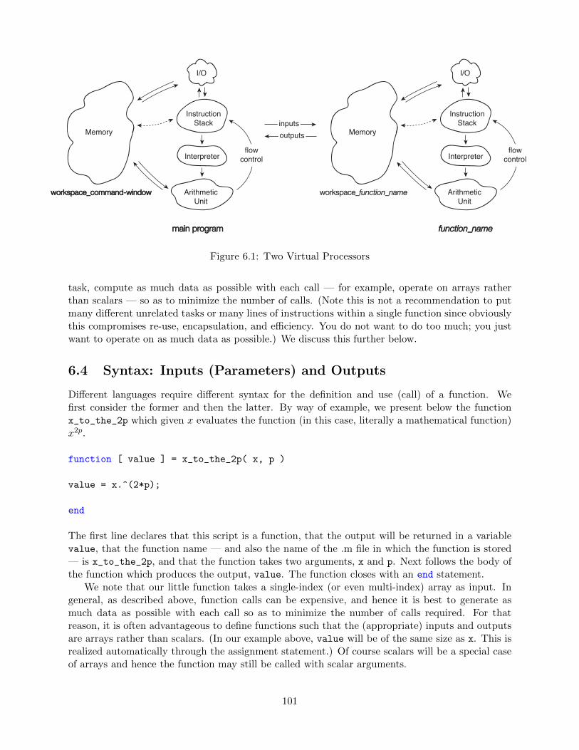
Memory

I/O

InstructionStack

Interpreter

ArithmeticUnit

flowcontrol

Memory

I/O

InstructionStack

Interpreter

ArithmeticUnit

flowcontrol

inputsoutputs

main programmain program function_namefunction_name

workspace_command-windowworkspace_command-window workspace_workspace_function_namefunction_name

Figure 6.1: Two Virtual Processors

task, compute as much data as possible with each call — for example, operate on arrays ratherthan scalars — so as to minimize the number of calls. (Note this is not a recommendation to putmany different unrelated tasks or many lines of instructions within a single function since obviouslythis compromises re-use, encapsulation, and efficiency. You do not want to do too much; you justwant to operate on as much data as possible.) We discuss this further below.

6.4 Syntax: Inputs (Parameters) and Outputs

Different languages require different syntax for the definition and use (call) of a function. Wefirst consider the former and then the latter. By way of example, we present below the functionx_to_the_2p which given x evaluates the function (in this case, literally a mathematical function)x2p.

function [ value ] = x_to_the_2p( x, p )

value = x.^(2*p);

end

The first line declares that this script is a function, that the output will be returned in a variablevalue, that the function name — and also the name of the .m file in which the function is stored— is x_to_the_2p, and that the function takes two arguments, x and p. Next follows the body ofthe function which produces the output, value. The function closes with an end statement.

We note that our little function takes a single-index (or even multi-index) array as input. Ingeneral, as described above, function calls can be expensive, and hence it is best to generate asmuch data as possible with each call so as to minimize the number of calls required. For thatreason, it is often advantageous to define functions such that the (appropriate) inputs and outputsare arrays rather than scalars. (In our example above, value will be of the same size as x. This isrealized automatically through the assignment statement.) Of course scalars will be a special caseof arrays and hence the function may still be called with scalar arguments.

101

More generally the syntax for a function with J inputs and K outputs is

function [output 1, output 2, . . . , output K] = function name(input 1, input 2, ..., input J)BODY of FUNCTIONend

Note that we may have not only multiple inputs but also multiple outputs. All outputs mustbe defined within the BODY of FUNCTION or Matlab will complain.

The operation of the function is fairly clear. First our little example (which we call here from thecommand window, but of course could also be called from a “main” program or another functionprogram):

>> clear all

>> y = x_to_the_2p( [1,2], 2)

y =

1 16

>> value

??? Undefined function or variable 'value'.>>

Note in the above our function is evaluated and the output assigned to the variable y. The variablevalue is internal to the function and the calling program — in this case the function is called fromthe command-line mode and hence the calling program variables are simply the workspace — hasno knowledge of this “dummy” variable.

More generally, we call a function with J outputs and K inputs as [output 1, output 2, . . . ,output J] = function name(input 1, input 2, . . . , input J); . (Note that if we omit the semi-colon then our outputs will all be displayed in the command window.) Upon being called bythe calling program, function name executes BODY of FUNCTION for the values of the inputarguments passed to function name and then upon reaching the end statement function namereturns the outputs — and control — to the calling program. Note is possible to force an earlyreturn of a function (to the calling program) before the end statement is encountered with a return

statement within the BODY of FUNCTION .It is possible to request only the first K ′ outputs as [output 1, output 2, . . . , output K′] =

function name(input 1, input 2, . . . , input J);. Particularly useful is the case in which you onlyrequire the first output, as in this case you can directly use the function through composition withina larger expression with the intermediary of assignment. Up to this point, with the exception of min,we have considered only single-output functions (or in any event only asked for the first output) inour examples — and for precisely this composition reason. Another example here:

>> z = x_to_the_2p( [1,2], 2) + [2,3]

z =

3 19

>>

102

Note it is important to distinguish between multiple outputs and arrays. An array corresponds toa particular output, not multiple outputs; in our example above, there is a single output, whichhappens to be a single-index array of length 2.

It is also possible to call a function without all inputs specified, either with [] (null) entries orsimply with a truncated list — the first J ′ inputs. However, in this case, it is important that withinthe function all inputs that will be encountered are defined. In this regard, the Matlab functionisempty is useful (for nulls) and the Matlab nargin is useful (for truncated argument lists)in order to detect any “unset” inputs which must be assigned to default values. (Note differentprogramming languages have different mechanisms for dealing with defaults.) There is also annargout Matlab function useful in tailoring the outputs provided.

6.5 Functions of Functions: Handles

It is often the case that we wish to pass a function to a function: in other words, we wish a calledfunction to be able to operate not just on different data but also on different “input functions.” Tomake matters more concrete (and avoid using the word function too many times with reference todifferent entities), consider the function f_o_diff:

function [ value ] = f_o_diff ( func, x, delta_x )

value = (func (x + delta_x) - func (x))./delta_x;

end

This little function calculates the first-order finite difference approximation to a function funcat the point x for a given segment-length delta_x. Obviously we could include the definition offunc within f_o_diff, but then we would need to have a different derivative function for eachfunction we wished to differentiate. In contrast, f_o_diff can be re-used for any function func— clearly much preferred. (Note we could now perform a much more systematic investigation ofround-off error; in our earlier discussion we were not yet armed with functions, or arrays.)

To call f_o_diff from a calling program is quite simple with only one wrinkle within theMatlab syntax. In particular, to pass the input function func from the calling program to thecalled function (f_o_diff) we do not wish to actually pass the function but rather a kind ofpointer — or handle — to where these instructions are stored for use by any (calling) program.(The description here is virtual — a mental model which provides the right intuition. In general,what and how a programming language passes within a function call can be a rather complicatedissue.) To create a handle for the function func — in other words, to find the pointer to (say) thebeginning of the set of instructions which define func — we put an “at sign” (@) in front of funcas in @func. So for example, to apply f_o_diff to the Matlab function sin we can either do

>> sin_handle = @sin;

>> fprime = f_o_diff( sin_handle, [pi/4, pi/2], .01)

fprime =

0.7036 -0.0050

>>

103

of more directly

>> fprime_too = f_o_diff( @sin, [pi/4, pi/2], .01)

fprime_too = 0.7036 -0.0050

>>

Note handles can also be created for other kinds of objects, for example (graphics) figures.It is often the case that a function func we wish to pass to (say) function name is somehow

more general — defined with respect to more inputs — than the functions which function nameexpects. In Matlab there is an easy way to deal with this common occurrence, which we nowdiscuss.

6.6 Anonymous (or In-Line) Functions

A Matlab “anonymous” (or in-line) function is a one-liner with a single output and multipleinputs that can be defined directly in the command window or indeed on the fly in any program(possibly another function). An anonymous function has a very important property: any variablesnot defined as inputs will be assigned the current values — at the time the anonymous functionis created — within the “variable space” (e.g., workspace) of the calling program (e.g., commandwindow).

We provide a concrete example. In particular, we define an anonymous function

p = 2;

x_to_the_2p_anon = @(x) x_to_the_2p(x,p);

which is identical to x_to_the_2p but now a function of single variable, x, rather than two variables.The value of p is frozen to 2, though of course more generally we can replace p = 2 with anyexpression by which to evaluate p in terms of other variables.

To call our anonymous function, we do (following the definition above):

>> x_to_the_2p_anon([1,2])

ans =

1 16

>>

The above appears rather pointless, but it serves an important role in passing functions to otherfunctions — in particular in the context of Matlab in which there are many built-in’s that requirefunction inputs of a particular form.

Let’s say that we wish to apply our function f_o_diff to our function x_to_the_2p. Butf_o_diff is expecting a function of a single input, x, whereas x_to_the_2p has two inputs — andtwo necessary inputs, since without p we can not evaluate x_to_the_2p. This conundrum is easilyresolved with inline functions:

104

>> p = 2;

>> x_to_the_2p_anon = @(x) x_to_the_2p(x,p);

>> z = f_o_diff( x_to_the_2p_anon, [1,2], .01 )

z =

4.0604 32.2408

>>

Note that for an in-line function the function “name” is in fact the function handle (hence we needno @ in front of the x_to_the_2p_anon in the above) — the name and handle for a single-linefunction coalesce.

6.7 String Inputs and the eval Function

We note that on occasion we do want the actual function to change — the instructions to beevaluated to change — as we change the inputs. This can be done with the eval function. Thefunction eval takes as input a string and returns the evaluation of this string given current valuesfor the various variables present in the string; in essence, eval is in the interpreter.

For example, we can create the function

function [ value ] = f_o_diff_eval ( fstring, x, delta_x )

z = x;

f_x = eval(fstring);

z = x + delta_x;

f_x_plus = eval(fstring);

value = (f_x_plus - f_x)./delta_x;

end

which is our finite difference function but now with a string input fstring to specify the functionto be differentiated. Note that eval(fstring) will simply evaluate the expression fstring giventhe current values of the workspace f o diff eval.

We now call f_o_diff_eval:

>> fstring = 'z.^4';>> f_o_diff_eval(fstring,[1,2],.01)

ans =

4.0604 32.2408

>>

which gives us the same result as previously. Note that f_x = eval(fstring) in f_o_diff_eval

105

for fstring as given is equivalent to f_x = z.^4 but since in the previous line we set z = x thenf_x is assigned x.^4 as desired. Similarly, two lines down, f_x_plus is assigned the appropriatevalue since we have changed z to be z = x + delta_x. The user can now specify any desiredfunction (expressed in terms of z) without creating a Matlab function (or anonymous function).

In actual practice there are certainly better ways to accomplish these goals. The purpose ofthis little section is only to illustrate that on occasions in which we would like to adapt the actualcode there are some simple ways to implement this feature.

106

Chapter 7

Integration

7.1 Integration of Univariate Functions

Our objective is to approximate the value of the integral

I =

∫ b

af(x) dx ,

for some arbitrary univariate function f(x). Our approach to this integration problem is to ap-proximate function f by an interpolant If and to exactly integrate the interpolant, i.e.

I =N−1∑i=1

∫Si

f(x) dx ≈N−1∑i=1

∫Si

(If)(x) dx ≡ Ih . (7.1)

Recall that in constructing an interpolant, we discretize the domain [a, b] into N−1 non-overlappingsegments, delineated by segmentation points xi, i = 1, . . . , N , as illustrated in Figure 7.11 Then,we construct a polynomial interpolant on each segment using the function values at the localinterpolation points, xm, m = 1, . . . ,M . These local interpolation points can be mapped to globalfunction evaluation points, xi, i = 1, . . . , Neval. The quality of the interpolant is dictated by its typeand the segment length h, which in turn governs the quality of the integral approximation, Ih. Thesubscript h on Ih signifies that the integration is performed on a discretization with a segment lengthh. This integration process takes advantage of the ease of integrating the polynomial interpolanton each segment.

Recalling that the error in the interpolation decreases with h, we can expect the approximationof the integral Ih to approach the true integral I as h goes to 0. Let us formally establish therelationship between the interpolation error bound, emax = maxi ei, and the integration error,

1For simplicity, we assume h is constant throughout the domain.

107

DRAFT V2.1 © The Authors. License: Creative Commons BY-NC-SA 3.0.

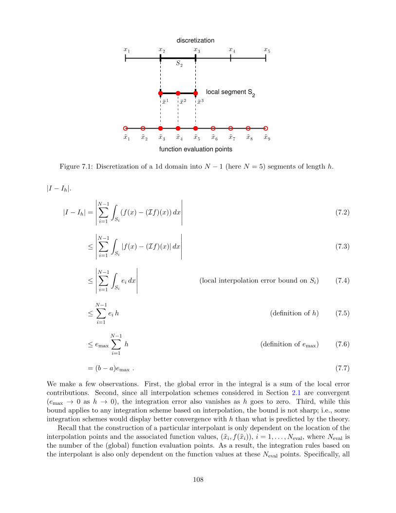
x1

x2

x3

x4

x5

S2

discretization

x1 x2 x3

local segment S2

x1

x2

x3

x4

x5

x6

x7

x8

x9

function evaluation points

Figure 7.1: Discretization of a 1d domain into N − 1 (here N = 5) segments of length h.

|I − Ih|.

|I − Ih| =

∣∣∣∣∣∣N−1∑i=1

∫Si

(f(x)− (If)(x)) dx

∣∣∣∣∣∣ (7.2)

≤

∣∣∣∣∣∣N−1∑i=1

∫Si

|f(x)− (If)(x)| dx

∣∣∣∣∣∣ (7.3)

≤

∣∣∣∣∣∣N−1∑i=1

∫Si

ei dx

∣∣∣∣∣∣ (local interpolation error bound on Si) (7.4)

≤N−1∑i=1

ei h (definition of h) (7.5)

≤ emax

N−1∑i=1

h (definition of emax) (7.6)

= (b− a)emax . (7.7)

We make a few observations. First, the global error in the integral is a sum of the local errorcontributions. Second, since all interpolation schemes considered in Section 2.1 are convergent(emax → 0 as h → 0), the integration error also vanishes as h goes to zero. Third, while thisbound applies to any integration scheme based on interpolation, the bound is not sharp; i.e., someintegration schemes would display better convergence with h than what is predicted by the theory.

Recall that the construction of a particular interpolant is only dependent on the location of theinterpolation points and the associated function values, (xi, f(xi)), i = 1, . . . , Neval, where Neval isthe number of the (global) function evaluation points. As a result, the integration rules based onthe interpolant is also only dependent on the function values at these Neval points. Specifically, all

108

integration rules considered in this chapter are of the form

Ih =

Neval∑i=1

wif(xi) ,

where wi are the weights associated with each point and are dependent on the interpolant fromwhich the integration rules are constructed. In the context of numerical integration, the functionevaluation points are called quadrature points and the associated weights are called quadratureweights. The quadrature points and weights together constitute a quadrature rule. Not too sur-prisingly considering the Riemann integration theory, the integral is approximated as a linearcombination of the function values at the quadrature points.

Let us provide several examples of integration rules.

Example 7.1.1 rectangle rule, leftThe first integration rule considered is a rectangle rule based on the piecewise-constant, left-endpoint interpolation rule considered in Example 2.1.1. Recall the interpolant over each segmentis obtained by approximating the value of the function by a constant function that matches thevalue of the function at the left endpoint, i.e., the interpolation point is x1 = xi on segmentSi = [xi, xi+1]. The resulting integration formula is

Ih =N−1∑i=1

∫Si

(If)(x) dx =N−1∑i=1

∫Si

f(xi) dx =N−1∑i=1

hf(xi) ,

where the piecewise-constant function results in a trivial integration. Recalling that the globalfunction evaluation points, xi, are related to the segmentation points, xi, by

xi = xi, i = 1, . . . , N − 1 ,

we can also express the integration rule as

Ih =

N−1∑i=1

hf(xi) .

Figure 7.2(a) illustrates the integration rule applied to f(x) = exp(x) over [0, 1] with N = 5. Recallthat for simplicity we assume that all intervals are of the same length, h ≡ xi+1−xi, i = 1, . . . , N−1.

Let us now analyze the error associated with this integration rule. From the figure, it is clearthat the error in the integrand is a sum of the local errors committed on each segment. The localerror on each segment is the triangular gap between the interpolant and the function, which hasthe length of h and the height proportional to f ′h. Thus, the local error scales as f ′h2. Since thereare (b− a)/h segments, we expect the global integration error to scale as

|I − Ih| ∼ f ′h2(b− a)/h ∼ hf ′ .

More formally, we can apply the general integration error bound, Eq. (7.7), to obtain

|I − Ih| ≤ (b− a)emax = (b− a)h maxx∈[a,b]

|f ′(x)| .

In fact, this bound can be tightened by a constant factor, yielding

|I − Ih| ≤ (b− a)h

2maxx∈[a,b]

|f ′(x)| .

109

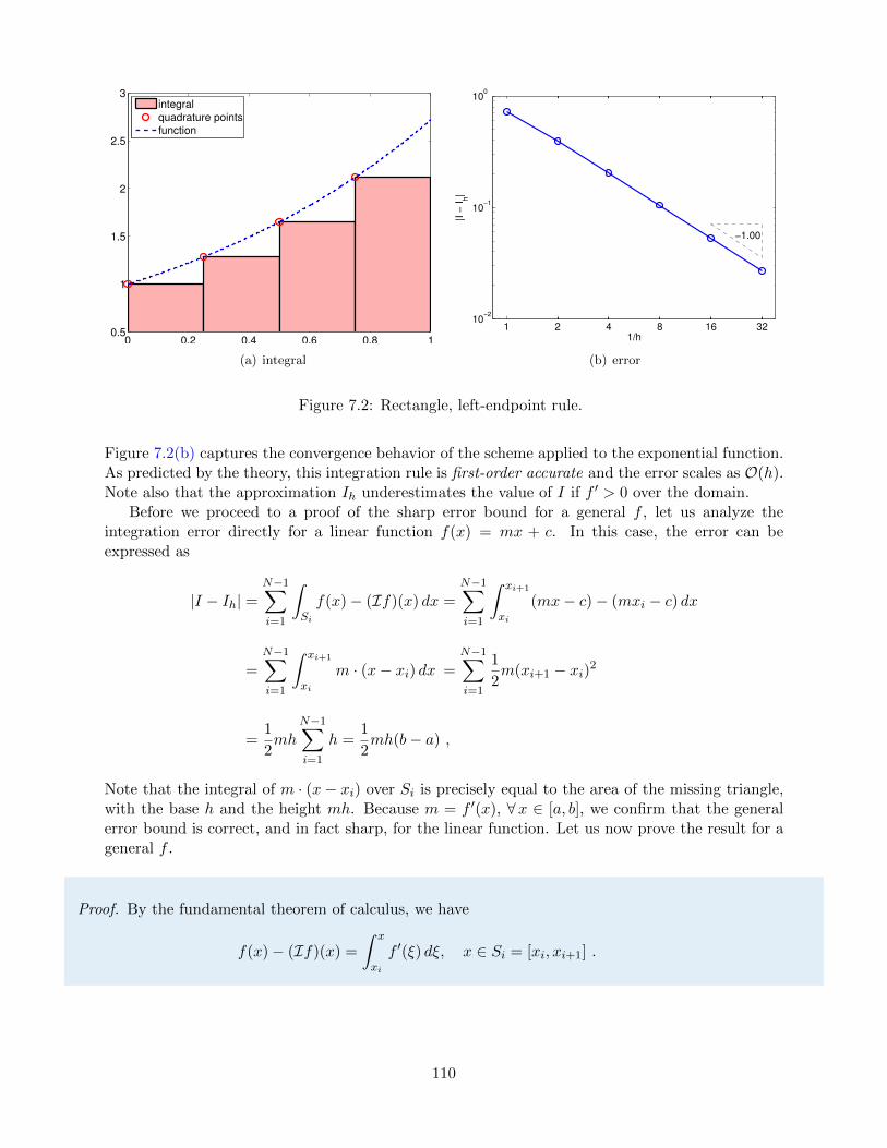
0 0.2 0.4 0.6 0.8 10.5

1

1.5

2

2.5

3

integral

quadrature points

function

(a) integral

1 2 4 8 16 3210

−2

10−1

100

−1.00

1/h

|I −

Ih|

(b) error

Figure 7.2: Rectangle, left-endpoint rule.

Figure 7.2(b) captures the convergence behavior of the scheme applied to the exponential function.As predicted by the theory, this integration rule is first-order accurate and the error scales as O(h).Note also that the approximation Ih underestimates the value of I if f ′ > 0 over the domain.

Before we proceed to a proof of the sharp error bound for a general f , let us analyze theintegration error directly for a linear function f(x) = mx + c. In this case, the error can beexpressed as

|I − Ih| =N−1∑i=1

∫Si

f(x)− (If)(x) dx =N−1∑i=1

∫ xi+1

xi

(mx− c)− (mxi − c) dx

=N−1∑i=1

∫ xi+1

xi

m · (x− xi) dx =N−1∑i=1

1

2m(xi+1 − xi)2

=1

2mh

N−1∑i=1

h =1

2mh(b− a) ,

Note that the integral of m · (x− xi) over Si is precisely equal to the area of the missing triangle,with the base h and the height mh. Because m = f ′(x), ∀x ∈ [a, b], we confirm that the generalerror bound is correct, and in fact sharp, for the linear function. Let us now prove the result for ageneral f .

Proof. By the fundamental theorem of calculus, we have

f(x)− (If)(x) =

∫ x

xi

f ′(ξ) dξ, x ∈ Si = [xi, xi+1] .

110

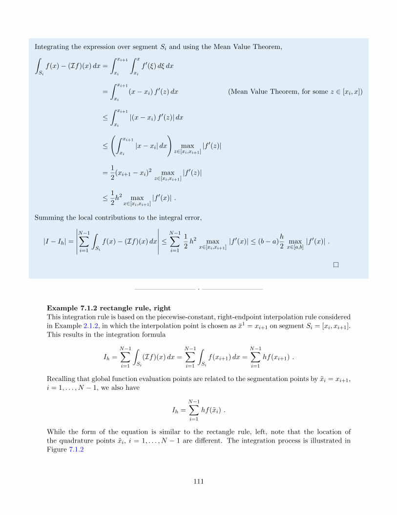
Integrating the expression over segment Si and using the Mean Value Theorem,∫Si

f(x)− (If)(x) dx =

∫ xi+1

xi

∫ x

xi

f ′(ξ) dξ dx

=

∫ xi+1

xi

(x− xi) f ′(z) dx (Mean Value Theorem, for some z ∈ [xi, x])

≤∫ xi+1

xi

|(x− xi) f ′(z)| dx

≤(∫ xi+1

xi

|x− xi| dx)

maxz∈[xi,xi+1]

|f ′(z)|

=1

2(xi+1 − xi)2 max

z∈[xi,xi+1]|f ′(z)|

≤ 1

2h2 max

x∈[xi,xi+1]|f ′(x)| .

Summing the local contributions to the integral error,

|I − Ih| =

∣∣∣∣∣∣N−1∑i=1

∫Si

f(x)− (If)(x) dx

∣∣∣∣∣∣ ≤N−1∑i=1

1

2h2 max

x∈[xi,xi+1]|f ′(x)| ≤ (b− a)

h

2maxx∈[a,b]

|f ′(x)| .

·

Example 7.1.2 rectangle rule, rightThis integration rule is based on the piecewise-constant, right-endpoint interpolation rule consideredin Example 2.1.2, in which the interpolation point is chosen as x1 = xi+1 on segment Si = [xi, xi+1].This results in the integration formula

Ih =

N−1∑i=1

∫Si

(If)(x) dx =

N−1∑i=1

∫Si

f(xi+1) dx =

N−1∑i=1

hf(xi+1) .

Recalling that global function evaluation points are related to the segmentation points by xi = xi+1,i = 1, . . . , N − 1, we also have

Ih =

N−1∑i=1

hf(xi) .

While the form of the equation is similar to the rectangle rule, left, note that the location ofthe quadrature points xi, i = 1, . . . , N − 1 are different. The integration process is illustrated inFigure 7.1.2

111

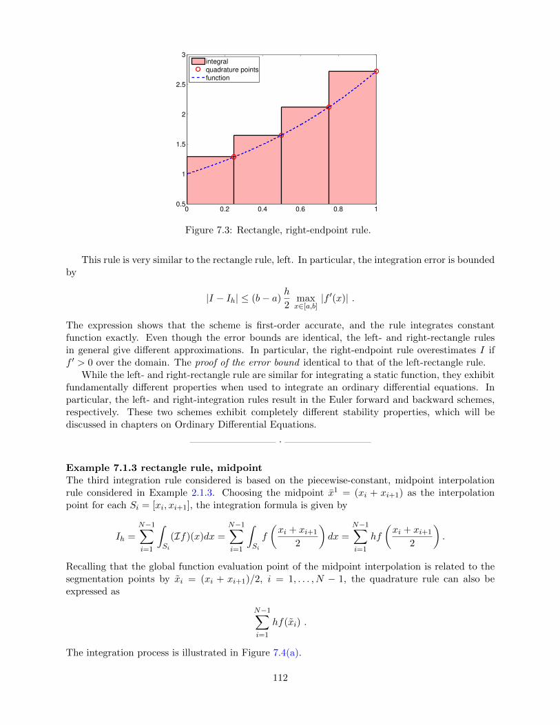
0 0.2 0.4 0.6 0.8 10.5

1

1.5

2

2.5

3

integral

quadrature points

function

Figure 7.3: Rectangle, right-endpoint rule.

This rule is very similar to the rectangle rule, left. In particular, the integration error is boundedby

|I − Ih| ≤ (b− a)h

2maxx∈[a,b]

|f ′(x)| .

The expression shows that the scheme is first-order accurate, and the rule integrates constantfunction exactly. Even though the error bounds are identical, the left- and right-rectangle rulesin general give different approximations. In particular, the right-endpoint rule overestimates I iff ′ > 0 over the domain. The proof of the error bound identical to that of the left-rectangle rule.

While the left- and right-rectangle rule are similar for integrating a static function, they exhibitfundamentally different properties when used to integrate an ordinary differential equations. Inparticular, the left- and right-integration rules result in the Euler forward and backward schemes,respectively. These two schemes exhibit completely different stability properties, which will bediscussed in chapters on Ordinary Differential Equations.

·

Example 7.1.3 rectangle rule, midpointThe third integration rule considered is based on the piecewise-constant, midpoint interpolationrule considered in Example 2.1.3. Choosing the midpoint x1 = (xi + xi+1) as the interpolationpoint for each Si = [xi, xi+1], the integration formula is given by

Ih =N−1∑i=1

∫Si

(If)(x)dx =N−1∑i=1

∫Si

f

(xi + xi+1

2

)dx =

N−1∑i=1

hf

(xi + xi+1

2

).

Recalling that the global function evaluation point of the midpoint interpolation is related to thesegmentation points by xi = (xi + xi+1)/2, i = 1, . . . , N − 1, the quadrature rule can also beexpressed as

N−1∑i=1

hf(xi) .

The integration process is illustrated in Figure 7.4(a).

112

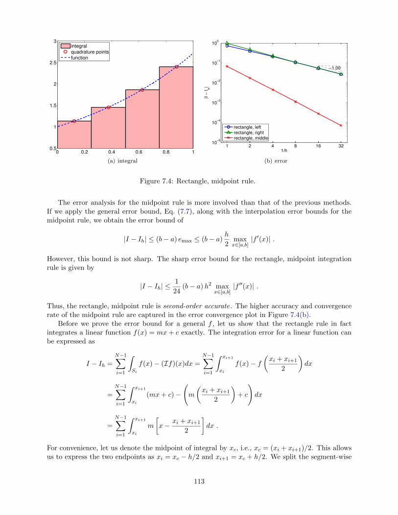
0 0.2 0.4 0.6 0.8 10.5

1

1.5

2

2.5

3

integral

quadrature points

function

(a) integral

1 2 4 8 16 3210

−5

10−4

10−3

10−2

10−1

100

−1.00

1/h

|I −

Ih|

rectangle, left

rectangle, right

rectangle, middle

(b) error

Figure 7.4: Rectangle, midpoint rule.

The error analysis for the midpoint rule is more involved than that of the previous methods.If we apply the general error bound, Eq. (7.7), along with the interpolation error bounds for themidpoint rule, we obtain the error bound of

|I − Ih| ≤ (b− a) emax ≤ (b− a)h

2maxx∈[a,b]

|f ′(x)| .

However, this bound is not sharp. The sharp error bound for the rectangle, midpoint integrationrule is given by

|I − Ih| ≤1

24(b− a)h2 max

x∈[a,b]|f ′′(x)| .

Thus, the rectangle, midpoint rule is second-order accurate. The higher accuracy and convergencerate of the midpoint rule are captured in the error convergence plot in Figure 7.4(b).

Before we prove the error bound for a general f , let us show that the rectangle rule in factintegrates a linear function f(x) = mx+ c exactly. The integration error for a linear function canbe expressed as

I − Ih =

N−1∑i=1

∫Si

f(x)− (If)(x)dx =N−1∑i=1

∫ xi+1

xi

f(x)− f(xi + xi+1

2

)dx

=N−1∑i=1

∫ xi+1

xi

(mx+ c)−(m

(xi + xi+1

2

)+ c

)dx

=

N−1∑i=1

∫ xi+1

xi

m

[x− xi + xi+1

2

]dx .

For convenience, let us denote the midpoint of integral by xc, i.e., xc = (xi + xi+1)/2. This allowsus to express the two endpoints as xi = xc − h/2 and xi+1 = xc + h/2. We split the segment-wise

113

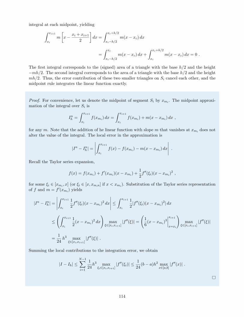
integral at each midpoint, yielding∫ xi+1

xi

m

[x− xi + xi+1

2

]dx =

∫ xc+h/2

xc−h/2m(x− xc) dx

=

∫ xc

xc−h/2m(x− xc) dx+

∫ xc+h/2

xc

m(x− xc) dx = 0 .

The first integral corresponds to the (signed) area of a triangle with the base h/2 and the height−mh/2. The second integral corresponds to the area of a triangle with the base h/2 and the heightmh/2. Thus, the error contribution of these two smaller triangles on Si cancel each other, and themidpoint rule integrates the linear function exactly.

Proof. For convenience, let us denote the midpoint of segment Si by xmi . The midpoint approxi-mation of the integral over Si is

Inh =

∫ xi+1

xi

f(xmi) dx =

∫ xi+1

xi

f(xmi) +m(x− xmi) dx ,

for any m. Note that the addition of he linear function with slope m that vanishes at xmi does notalter the value of the integral. The local error in the approximation is

|In − Inh | =∣∣∣∣∣∫ xi+1

xi

f(x)− f(xmi)−m(x− xmi) dx∣∣∣∣∣ .

Recall the Taylor series expansion,

f(x) = f(xmi) + f ′(xmi)(x− xmi) +1

2f ′′(ξi)(x− xmi)2 ,

for some ξi ∈ [xmi , x] (or ξi ∈ [x, xm,n] if x < xmi). Substitution of the Taylor series representationof f and m = f ′(xmi) yields

|In − Inh | =∣∣∣∣∣∫ xi+1

xi

1

2f ′′(ξi)(x− xmi)2 dx

∣∣∣∣∣ ≤∫ xi+1

xi

1

2|f ′′(ξi)(x− xmi)2| dx

≤(∫ xi+1

xi

1

2(x− xmi)2 dx

)max

ξ∈[xi,xi+1]|f ′′(ξ)| =

(1

6(x− xmi)3

∣∣∣∣xi+1

x=xi

)max

ξ∈[xi,xi+1]|f ′′(ξ)|

=1

24h3 max

ξ∈[xi,xi+1]|f ′′(ξ)| .

Summing the local contributions to the integration error, we obtain

|I − Ih| ≤N−1∑i=1

1

24h3 max

ξi∈[xi,xi+1]|f ′′(ξi)| ≤

1

24(b− a)h2 max

x∈[a,b]|f ′′(x)| .

114

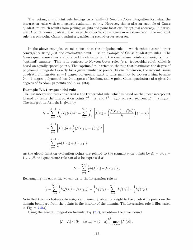
The rectangle, midpoint rule belongs to a family of Newton-Cotes integration formulas, theintegration rules with equi-spaced evaluation points. However, this is also an example of Gaussquadrature, which results from picking weights and point locations for optimal accuracy. In partic-ular, k point Gauss quadrature achieves the order 2k convergence in one dimension. The midpointrule is a one-point Gauss quadrature, achieving second-order accuracy.

·In the above example, we mentioned that the midpoint rule — which exhibit second-order

convergence using just one quadrature point — is an example of Gauss quadrature rules. TheGauss quadrature rules are obtained by choosing both the quadrature points and weights in an“optimal” manner. This is in contrast to Newton-Cotes rules (e.g. trapezoidal rule), which isbased on equally spaced points. The “optimal” rule refers to the rule that maximizes the degree ofpolynomial integrated exactly for a given number of points. In one dimension, the n-point Gaussquadrature integrates 2n − 1 degree polynomial exactly. This may not be too surprising because2n − 1 degree polynomial has 2n degrees of freedom, and n-point Gauss quadrature also gives 2ndegrees of freedom (n points and n weights).

Example 7.1.4 trapezoidal ruleThe last integration rule considered is the trapezoidal rule, which is based on the linear interpolantformed by using the interpolation points x1 = xi and x2 = xi+1 on each segment Si = [xi, xi+1].The integration formula is given by

Ih =N−1∑i=1

∫Si

(If)(x) dx =N−1∑i=1

∫Si

[f(xi) +

(f(xi+1)− f(xi)

h

)(x− xi)

]

=

N−1∑i=1

[f(xi)h+

1

2(f(xi+1)− f(xi))h

]

=N−1∑i=1

1

2h(f(xi) + f(xi+1)) .

As the global function evaluation points are related to the segmentation points by xi = xi, i =1, . . . , N , the quadrature rule can also be expressed as

Ih =

N−1∑i=1

1

2h(f(xi) + f(xi+1)) ,

Rearranging the equation, we can write the integration rule as

Ih =N−1∑i=1

1

2h(f(xi) + f(xi+1)) =

1

2hf(x1) +

N−1∑i=2

[hf(xi)

]+

1

2hf(xN ) .

Note that this quadrature rule assigns a different quadrature weight to the quadrature points on thedomain boundary from the points in the interior of the domain. The integration rule is illustratedin Figure 7.5(a).

Using the general integration formula, Eq. (7.7), we obtain the error bound

|I − Ih| ≤ (b− a)emax = (b− a)h2

8maxx∈[a,b]

|f ′′(x)| .

115

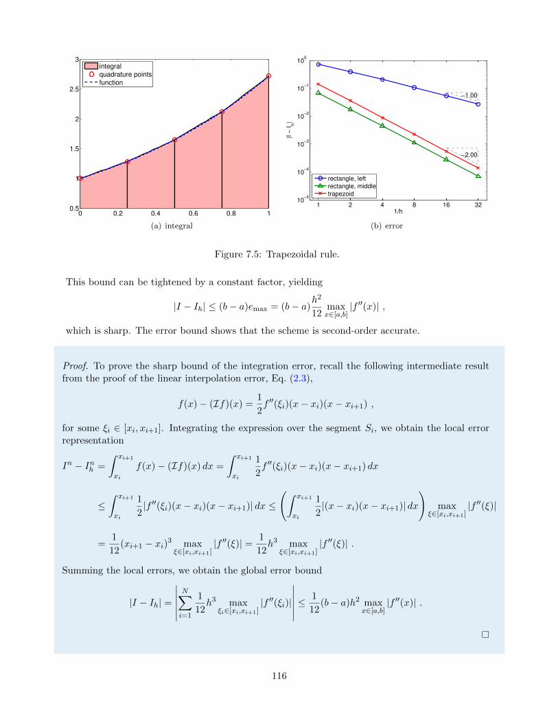
0 0.2 0.4 0.6 0.8 10.5

1

1.5

2

2.5

3

integral

quadrature points

function

(a) integral

1 2 4 8 16 3210

−5

10−4

10−3

10−2

10−1

100

−1.00

−2.00

1/h

|I −

Ih|

rectangle, left

rectangle, middle

trapezoid

(b) error

Figure 7.5: Trapezoidal rule.

This bound can be tightened by a constant factor, yielding

|I − Ih| ≤ (b− a)emax = (b− a)h2

12maxx∈[a,b]

|f ′′(x)| ,

which is sharp. The error bound shows that the scheme is second-order accurate.

Proof. To prove the sharp bound of the integration error, recall the following intermediate resultfrom the proof of the linear interpolation error, Eq. (2.3),

f(x)− (If)(x) =1

2f ′′(ξi)(x− xi)(x− xi+1) ,

for some ξi ∈ [xi, xi+1]. Integrating the expression over the segment Si, we obtain the local errorrepresentation

In − Inh =

∫ xi+1

xi

f(x)− (If)(x) dx =

∫ xi+1

xi

1

2f ′′(ξi)(x− xi)(x− xi+1) dx

≤∫ xi+1

xi

1

2|f ′′(ξi)(x− xi)(x− xi+1)| dx ≤

(∫ xi+1

xi

1

2|(x− xi)(x− xi+1)| dx

)max

ξ∈[xi,xi+1]|f ′′(ξ)|

=1

12(xi+1 − xi)3 max

ξ∈[xi,xi+1]|f ′′(ξ)| = 1

12h3 max

ξ∈[xi,xi+1]|f ′′(ξ)| .

Summing the local errors, we obtain the global error bound

|I − Ih| =

∣∣∣∣∣∣N∑i=1

1

12h3 max

ξi∈[xi,xi+1]|f ′′(ξi)|

∣∣∣∣∣∣ ≤ 1

12(b− a)h2 max

x∈[a,b]|f ′′(x)| .

116

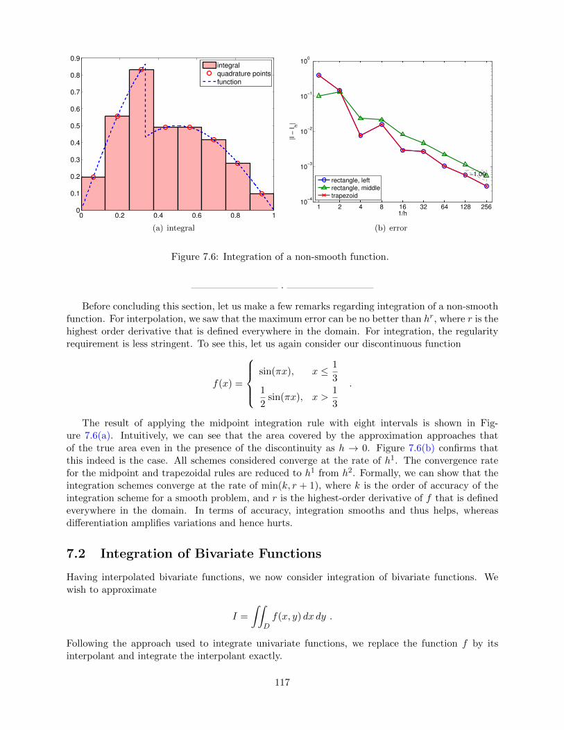
0 0.2 0.4 0.6 0.8 10

0.1

0.2

0.3

0.4

0.5

0.6

0.7

0.8

0.9

integralquadrature pointsfunction

(a) integral

1 2 4 8 16 32 64 128 25610

−4

10−3

10−2

10−1

100

−1.00

1/h

|I −

Ih|

rectangle, left

rectangle, middle

trapezoid

(b) error

Figure 7.6: Integration of a non-smooth function.

·Before concluding this section, let us make a few remarks regarding integration of a non-smooth

function. For interpolation, we saw that the maximum error can be no better than hr, where r is thehighest order derivative that is defined everywhere in the domain. For integration, the regularityrequirement is less stringent. To see this, let us again consider our discontinuous function

f(x) =

sin(πx), x ≤ 1

31

2sin(πx), x >

1

3

.

The result of applying the midpoint integration rule with eight intervals is shown in Fig-ure 7.6(a). Intuitively, we can see that the area covered by the approximation approaches thatof the true area even in the presence of the discontinuity as h → 0. Figure 7.6(b) confirms thatthis indeed is the case. All schemes considered converge at the rate of h1. The convergence ratefor the midpoint and trapezoidal rules are reduced to h1 from h2. Formally, we can show that theintegration schemes converge at the rate of min(k, r + 1), where k is the order of accuracy of theintegration scheme for a smooth problem, and r is the highest-order derivative of f that is definedeverywhere in the domain. In terms of accuracy, integration smooths and thus helps, whereasdifferentiation amplifies variations and hence hurts.

7.2 Integration of Bivariate Functions

Having interpolated bivariate functions, we now consider integration of bivariate functions. Wewish to approximate

I =

∫∫Df(x, y) dx dy .

Following the approach used to integrate univariate functions, we replace the function f by itsinterpolant and integrate the interpolant exactly.

117

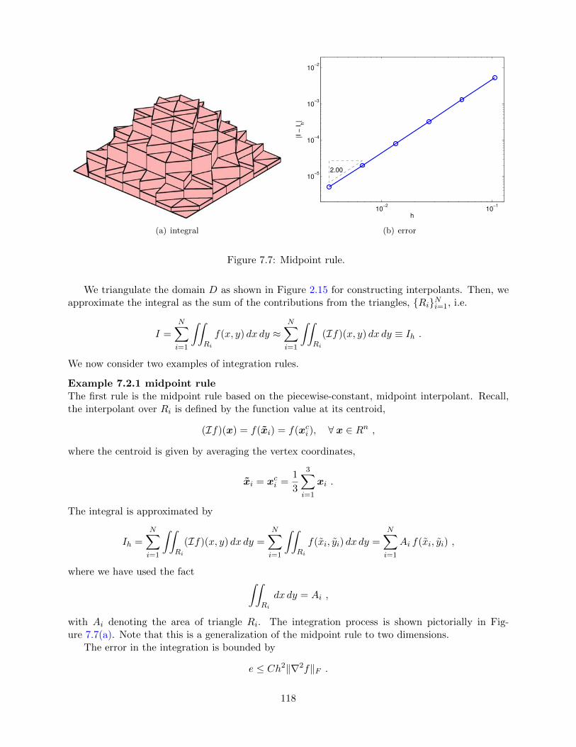
(a) integral

10−2

10−1

10−5

10−4

10−3

10−2

2.00

h

|I −

Ih|

(b) error

Figure 7.7: Midpoint rule.

We triangulate the domain D as shown in Figure 2.15 for constructing interpolants. Then, weapproximate the integral as the sum of the contributions from the triangles, {Ri}Ni=1, i.e.

I =

N∑i=1

∫∫Ri

f(x, y) dx dy ≈N∑i=1

∫∫Ri

(If)(x, y) dx dy ≡ Ih .

We now consider two examples of integration rules.

Example 7.2.1 midpoint ruleThe first rule is the midpoint rule based on the piecewise-constant, midpoint interpolant. Recall,the interpolant over Ri is defined by the function value at its centroid,

(If)(x) = f(xi) = f(xci ), ∀ x ∈ Rn ,

where the centroid is given by averaging the vertex coordinates,

xi = xci =1

3

3∑i=1

xi .

The integral is approximated by

Ih =N∑i=1

∫∫Ri

(If)(x, y) dx dy =

N∑i=1

∫∫Ri

f(xi, yi) dx dy =

N∑i=1

Ai f(xi, yi) ,

where we have used the fact ∫∫Ri

dx dy = Ai ,

with Ai denoting the area of triangle Ri. The integration process is shown pictorially in Fig-ure 7.7(a). Note that this is a generalization of the midpoint rule to two dimensions.

The error in the integration is bounded by

e ≤ Ch2‖∇2f‖F .

118

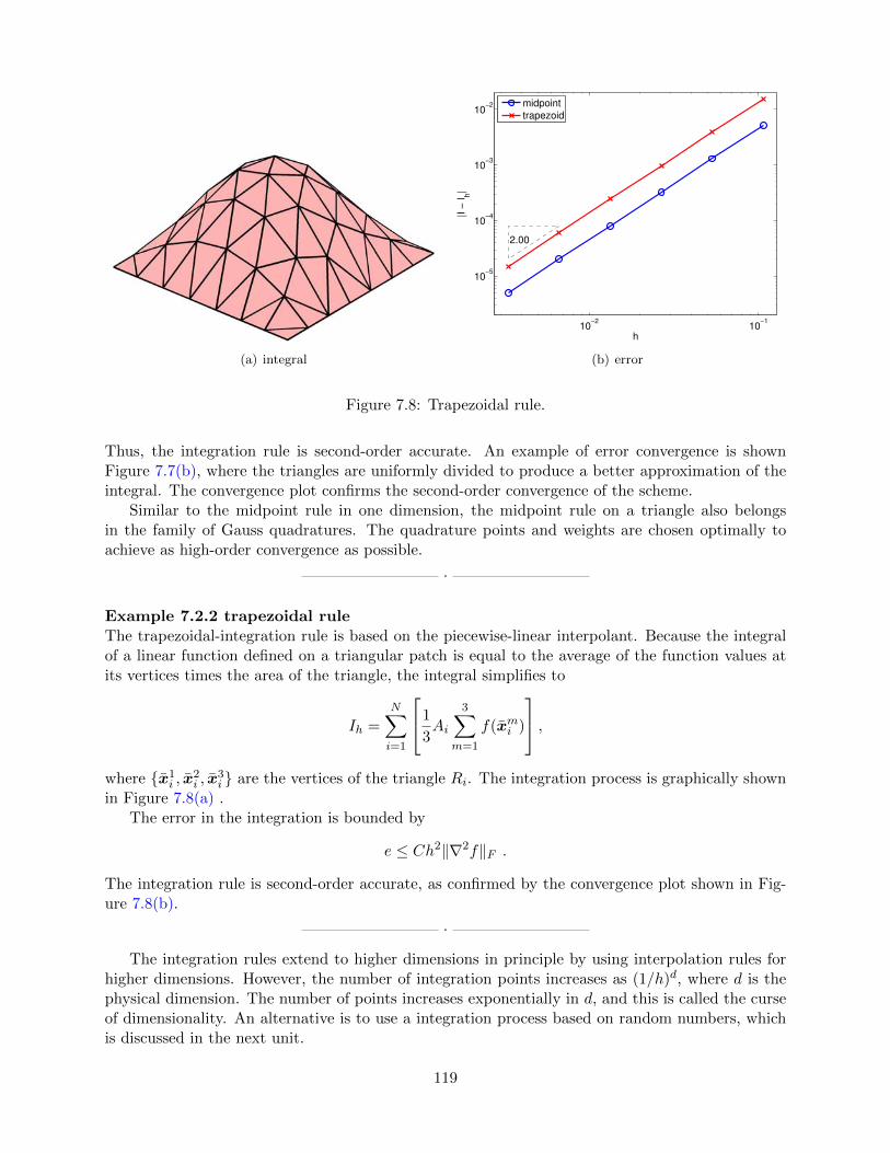
(a) integral

10−2

10−1

10−5

10−4

10−3

10−2

2.00

h

|I −

Ih|

midpoint

trapezoid

(b) error

Figure 7.8: Trapezoidal rule.

Thus, the integration rule is second-order accurate. An example of error convergence is shownFigure 7.7(b), where the triangles are uniformly divided to produce a better approximation of theintegral. The convergence plot confirms the second-order convergence of the scheme.

Similar to the midpoint rule in one dimension, the midpoint rule on a triangle also belongsin the family of Gauss quadratures. The quadrature points and weights are chosen optimally toachieve as high-order convergence as possible.

·

Example 7.2.2 trapezoidal ruleThe trapezoidal-integration rule is based on the piecewise-linear interpolant. Because the integralof a linear function defined on a triangular patch is equal to the average of the function values atits vertices times the area of the triangle, the integral simplifies to

Ih =N∑i=1

1

3Ai

3∑m=1

f(xmi )

,where {x1

i , x2i , x

3i } are the vertices of the triangle Ri. The integration process is graphically shown

in Figure 7.8(a) .The error in the integration is bounded by

e ≤ Ch2‖∇2f‖F .

The integration rule is second-order accurate, as confirmed by the convergence plot shown in Fig-ure 7.8(b).

·The integration rules extend to higher dimensions in principle by using interpolation rules for

higher dimensions. However, the number of integration points increases as (1/h)d, where d is thephysical dimension. The number of points increases exponentially in d, and this is called the curseof dimensionality. An alternative is to use a integration process based on random numbers, whichis discussed in the next unit.

119

120

MIT OpenCourseWarehttp://ocw.mit.edu

2.086 Numerical Computation for Mechanical EngineersSpring 2013

For information about citing these materials or our Terms of Use, visit: http://ocw.mit.edu/terms.