Chapter 1 Systems of Linear Equations

Elementary Row Operations

(I) Interchange two equations

(II) Multiply one equation by a nonzero number

(III) Add a multiple of one equation to a diff. equation

Theorem 1.1.1

Suppose that a sequence of elementary equations is performed

on a system of linear equations. Then the resulting system has

the same set of solutions as the original, so the two systems are

equivalent.

Row-echelon form

1. All zero rows (consisting entirely of zeros) are at the bottom

2. The first nonzero entry from the left in each nonzero row is

a 1, called the leading 1 for that row

3. Each leading 1 is to the right of all leading 1s in the rows

above it.

(Reduced row-echelon form)

4. Each leading 1 is the only nonzero entry in its column.

Theorem 1.2.1

Every matrix can be brought to (reduced) row-echelon form by

a sequence of elementary row operations.

Rank: The rank if matrix A is the number of leading 1s in any

row-echelon matrix to which A can be carried by row

operations

Theorem 1.2.2

Suppose a system of m equations in n variables is consistent,

and that the rank of the augmented matrix is r.

(1) The set of solutions involves exactly n-r parameters.

(2) If r<n, the system has infinitely many solutions.

(3) If r=n, the system has a unique solution.

Homogeneous Equations

If the equation has the form of “a1x1 + a2x2 + … + anxn = 0”,

clearly x1 = 0, x2 = 0, xn = 0 is a solution to such a system; it is

called trivial solution. Any solution in which at least one

variable has nonzero value is called a nontrivial solution.

Theorem 1.3.1

If a homogeneous system of linear equations has more

variables than equations, then it has a nontrivial solution (in

fact, infinitely many).

Linear combination

sx + ty (s, t arbitrary)

Any linear combination of solutions to a homogeneous system

is again a solution.

Basic solutions

The Gaussian algorithm systematically produces solutions to

any homogeneous linear system, called basic solution, one for

every parameter.

Any nonzero scalar multiple of a multiple of a basic solution

Theorem 1.3.2

Let A be an m x n matrix of rank r, and consider the

homogeneous system in n variables with A as coefficient

matrix. Then:

(1) The system has exactly n – r basic solutions, one for each

parameter.

(2) Every solution is a linear combination of these basic

solutions.

Chapter 2 Martix and Algebra

Theorem 2.1.1

Let A, B and C denote arbitrary m x n matrices where m and n

are fixed. Let k and p denote arbitrary real numbers. Then

A + B = B + A

A + (B + C) = (A + B) + C

There is an m x n matrix 0, such that 0 + A = A for each A

For each A there is an m x n matrix, -A, such that A + (-A) = 0

k(A + B) = kA + kB

(k + p)A = kA + pA

(kp)A = k(pA)

1A = A

Theorem 2.1.2

Let A and B denote matrices of the same size, and let k denote

a scalar.

If A is an m x n matrix, then AT is an n x m matrix.

(AT)T = A

(kA)T = kAT

(A + B)T = AT + BT

Let R denote the set of all real numbers. The set of all

ordered n-tuples from R has a special notation:

Rn denotes the set of all ordered n-tuples of real numbers.

(n-)Vectors: (r1, r2, …, rn) or columns [r1 r2 … rn]T

Theorem 2.2.1

(1) Every system of linear equations has the form Ax = b

where A is the coefficient matrix, b is the constant matrix, and

X is the matrix of variables.

(2) The system Ax = b is consistent if and only if b is a linear

combination of the columns of A.

(3) If a1, a2, …, an are the columns of A and if x = [x1 x2 … xn],

then x is a solution to the linear system Ax = b if and only if

x1, x2, … xn are a solution of the vector equation

x1a1 + x1a2 + … + xnan = b.

Theorem 2.2.2

Let A and B be m x n matrices, and let x and y be n-vectors in

Rn. Then:

(1) A(x + y) = Ax + Ay

(2) A(ax) = a(Ax) = (aA)x for all scalars a.

(3) (A + B)x = Ax + Bx

Theorem 2.2.3

Suppose x1 is any particular solution to the system Ax = b of

linear equations. Then every solution x2 has the form

x2 = x0 + x1, for some solution x0 of the associated

homogeneous system Ax = 0

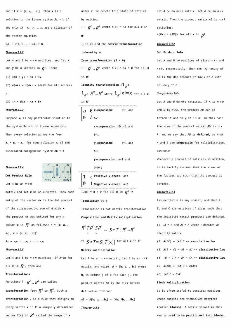
Theorem 2.2.4

Dot Product Rule

Let A be an m x n matrix

and let x be an n-vector. Then each entry of the vector Ax is

the dot product of the corresponding row of A with x.

The product Ax was defined for any n-column x in Rn as

follows: A = [a1 a2 … an], x = [x1 x2 … xn]T,

Ax = x1a1 + x1a2 + … + xnan

Theorem 2.2.5

Let A and B be m x n matrices. If A=Bx for all x in Rn, then

A=B

Transformations

Functions T: Rn → Rm are called transformation from

Rn to Rm

. Such a transformation T is a rule that assigns to

every vector x in Rn a uniquely determined vector T(x) in Rm

called the image of x under T. We denote this state of affairs

by writing

T : Rn → Rm where T(x) = Ax for all x in Rn

TA is called the matrix transformation induced by A.

Zero transformation (T = 0):

T : Rn → Rm where T(x) = Ax = 0 for all x in Rn

Identity transformation (1Rn):

1Rn: Rn → Rn where 1Rn ( x )=x for all x in Rn

[a 00 b]x-expansion: a>1 and b=1

x-compression: 0<a<1 and b=1

y-expansion: a=1 and b>1

y-compression: a=1 and 0<b<1

[1 c0 1] Positive x-shear: a>0

Negative x-shear: a<0

Tw(x) = x + w for all x in Rn Translation by w

Translation is not matrix transformation

Composition and Matrix Multiplication

Rk T→

Rn S→

Rm => S∘T : Rk → Rm

=> S∘T=S [T (x)] for all x in Rk

Matrix multiplication

Let A be an m x n matrix, let B be an n x k matrix, and write B

= [b1 b2 … bk] where bj is column j of B for each j. The

product matrix AB is the m x k matrix defined as follows:

AB = A[b1 b2 … bk] = [Ab1 Ab2 … Abk]

Theorem 2.3.1

Let A be an m x n matrix, let B be an n x k matrix. Then the

product matrix AB is m x k satisfies:

A(Bx) = (AB)x for all x in Rk

Theorem 2.3.2

Dot Product Rule

Let A and B be matrices of sizes m x n and n x k, respectively.

Then the (i,j)-entry of AB is the dot product of row I of A with

column j of B.

Compatibility Rule

Let A and B denote matrices. If A is m x n and B is n’ x k, the

product AB can be formed if and only if n = n’. In this case the

size of the product matrix AM is m x k, and we say that AB is

defined, or that A and B are compatible for multiplication.

Convention

Whenever a product of matrices is written, it is tacitly assumed

that the sizes of the factors are such that the product is defined.

Theorem 2.3.3

Assume that a is any scalar, and that A, B, and C are matrices

of sizes such that the indicated matrix products are defined.

(1) IA = A and AI = A where I denotes an identity matrix.

(2) A(BC) = (AB)C => associative law

(3) A(B + C) = AB + AC => distributive law

(4) (B + C)A = BA + CA => distributive law

(5) a(AB) = (aA)B = a(AB)

(6) (AB)T = BTAT

Block Multiplication

It is often useful to consider matrices whose entries are

themselves matrices (called blocks). A matrix viewed in this

way is said to be partitioned into blocks.

Theorem 2.3.4

Block Multiplication

If matrices A and B are partitioned compatibly into blocks, the

product AB can be computed by matrix multiplication using

blocks as entries

Theorem 2.3.5

Suppose matrices A=[B X0 C ] and

A1=[B1 X1

0 C1] are

partitioned as shown where B and B1 are square matrices of the

same size, and C and C1 are also square of the same size.

These are compatible partitionings and block multiplication

gives

A A1=[B X0 C ] [B1 X1

0 C1]=[BB1 B X1+X C1

0 C C1]

.

Theorem 2.3.6

If A is the adjacency matrix of a directed graph with n vertices,

then the (i,j)-entry of Ar is the number of r-paths vjvr.

A directed graph consists of a set of points (called vertices)

connected by arrows (called edges). For example, the vertices

could represent cities and the edges available flights. If the

graph has n vertices v1, v2, …, vn, the adjacency matrix A=[aij]

is the n x n matrix whose (i,j)-entry aij is 1 if there is an edge

from vj to vi (note the order), and zero otherwise.

Inverse

A matrix A that has an inverse is called an invertible matrix.

B is inverse of A if and only if AB = I and BA = I.

Theorem 2.4.1

If B and C are both inverses of A, then B = C

Theorem 2.4.2

Suppose a system of n equations in n variables is written in

matrix form as Ax = b. If the n x n coefficient matrix A is

invertible, the system has the unique solution x = A-1b.

det [a bc d ]=ad−bc , adj [a b

c d ]=[ d −b−c a ]

, A−1= 1

detAadjA

Matrix Inversion Algorithm

If A is an invertible (square) matrix there exists a sequence of

elementary row operations that carry A to the identity matrix I

of the same size, written AI. This same series of row

operations carries I to A-1; that is, IA-1. [A I][I A-1] where

the row operations on A and I are carried out simultaneously.

Theorem 2.4.3

If A is an n x n matrix, either A can be reduced to I by

elementary row operations or it cannot. In the first case, the

algorithm produces A-1; in the second case, A-1 does not exist.

Theorem 2.4.4

All of the following matrices are square matrices of the same

size.

(1) I is invertible and I-1 = I

(2) If A is invertible, so is A-1, and (A-1)-1 = A

(3) If A and B are invertible, so is AB, and (AB)-1 = B-1A-1

(4) If A1, A2, …, Ak are all invertible, so is their product A1A2…

Ak, and (A1A2…Ak)-1 = Ak-1…A2

-1A1-1.

(5) If A is invertible, so is Ak for any k ≥ 1, and (Ak)-1 = (A-1)k

(6) If A is invertible and a ≠ 0 is a number, then aA is

invertible and (aA)-1 = (1/a)A-1.

(7) If A is invertible, so is its transpose AT, and (AT)-1 = (A-1)T.

Corollary

A square matrix A is invertible if and only if AT is invertible.

Theorem 2.4.5

Inverse Theorem

The following conditions are equivalent for an n x n matrix A:

(1) A is invertible

(2) The homogeneous system Ax = 0 has only the trivial

solution x = 0

(3) A can be carried to the identity matrix In by ERO.

(4) The system Ax = b has at least one solution x for every

choice of column b.

(5) There exists an n x n matrix C such that AC = In.

Corollary 1: If A and C are matrices such that AC = I, then also

CA = I, In particular, both A and C are invertible, C = A-1 and A

= C-1.

Corollary 2: An n x n matrix A is invertible iff rank A = n.

Let P=[A X0 B ] and Q=[A 0

Y B] block

matrices where A is

m x m and B is n x n (possible m ≠n).

Q: Show that P is invertible iff A and B are both invertible. In

this case, show that P−1=[A−1 −A1 X B1

0 B1 ].

If A-1 and B-1 both exist, write

R=[A−1 −A1 X B1

0 B1 ]. Using

block multiplication, one verifies that PR = Im+n = RP, so P is

invertible, and P-1=R. Conversely, suppose that P is invertible,

and P−1=[ C VW D ] in block form, where is m x m and

D is

n x n. Then the equation PP-1 = In+m becomes

[A X0 B ][ C V

W D ]=[AC+ XW AV +XDBW BD ]=I m+n=[ I m 0

0 I n]

using block notation. Equating the corresponding blocks, we

find AC + XW = Im, BW = 0, and BD = In.

Hence B is invertible because BD = In (by Corollary 1), then

W = 0 because BW = 0, and finally, AC = Im (so A is invertible,

again by Corollary 1).

Inverse of Matrix transformation

Let T '=T A−1 :Rn→ Rn denote the transformation

induced by A-1. Then:

T ' [T ( x ) ]=A−1 [ A x ]=I x=xfor all x in Rn (*)

T [T ' (x ) ]=A [ A−1 x ]=I x=x

T carries x to a vector T(x) and T’ carries T(x) back to x, T’

reverses the action of T.

T '∘T=1Rn andT ∘T '=1R n (**)

When these conditions hold, the matrix transformation T’ is an

inverse T,

Theorem 2.4.6

Let T: Rn → Rn denote the matrix transformation induced

by an n x n matrix A. Then A is invertible if and only if T has

an inverse. In this case, T has exactly one inverse (denoted as

T-1), and T-1: Rn → Rn is the transformation induced by

the matrix A-1. In other words, (T A)−1=T A−1

.

Fundamental Identities:

T−1 [T (x ) ]=xandT [T−1 ( x ) ]=x for all x in Rn

(1) Let T be the linear transformation induced by A.

(2) Obtain the linear transformation T-1 which “reverses” the

action of T.

(3) Then A-1 is the matrix of T-1.

Elementary Matrices

An n x n matrix E is called an elementary matrix if it can be

obtained from the identity matrix In by a single elementary row

operation (called the operation corresponding to E). We say

that E is of type I, II, or III if the operation is of that type.

Lemma 1: If an elementary row operation is performed on an

m x n matrix A, the result is EA where E is the elementary

matrix obtained by performing the same operation on the m x

m identity matrix.

Lemma 2: Every elementary matrix E is invertible, and E-1 is

also a elementary matrix (of the same type). Moreover, E-1

corresponds to the inverse of the row operation that produce E.

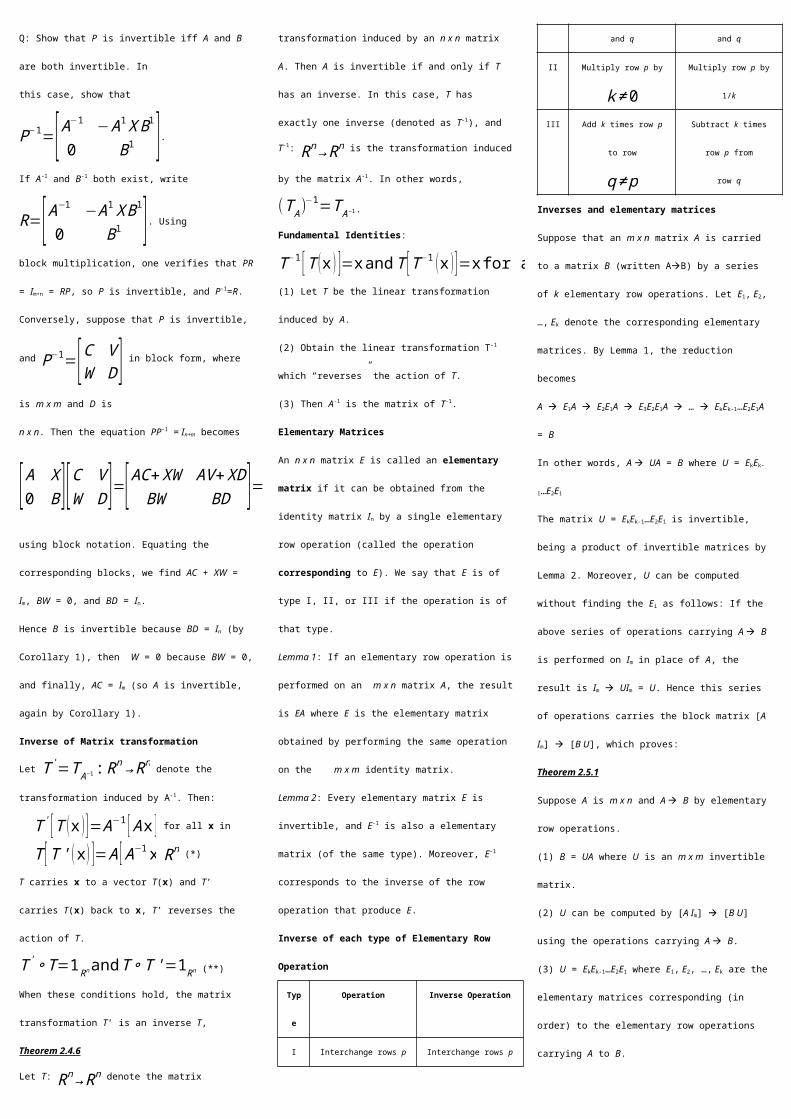
Inverse of each type of Elementary Row Operation

Type Operation Inverse Operation

I Interchange rows p and q Interchange rows p and q

IIMultiply row p by k ≠ 0 Multiply row p by 1/k

III Add k times row p to row

q ≠ p

Subtract k times row p from

row q

Inverses and elementary matrices

Suppose that an m x n matrix A is carried to a matrix B (written

AB) by a series of k elementary row operations. Let E1, E2,

…, Ek denote the corresponding elementary matrices. By

Lemma 1, the reduction becomes

A E1A E2E1A E3E2E1A … EkEk-1…E2E1A = B

In other words, A UA = B where U = EkEk-1…E2E1

The matrix U = EkEk-1…E2E1 is invertible, being a product of

invertible matrices by Lemma 2. Moreover, U can be

computed without finding the Ei as follows: If the above series

of operations carrying A B is performed on Im in place of A,

the result is Im UIm = U. Hence this series of operations

carries the block matrix [A Im] [B U], which proves:

Theorem 2.5.1

Suppose A is m x n and A B by elementary row operations.

(1) B = UA where U is an m x m invertible matrix.

(2) U can be computed by [A Im] [B U] using the operations

carrying A B.

(3) U = EkEk-1…E2E1 where E1, E2, …, Ek are the elementary

matrices corresponding (in order) to the elementary row

operations carrying A to B.

By theorem 2.5.1 (3), it gives A-1 = U = EkEk-1…E2E1, Hence

A = (A-1)-1 = (EkEk-1…E2E1)-1 = E1-1E2

-1… Ek-1-1Ek

-1

And by Lemma 2, every invertible matrix is a product of

elementary matrices and elementary matrices are invertible:

Theorem 2.5.2

A square matrix is invertible if and only if it is a product of

elementary matrices.

Smith Normal Form

Let A be an m x n matrix of rank r, and let R be the reduced

row-echelon form of A. Theorem 2.5.1 shows that R = UA

where U is invertible, and that U can be found from

[A Im] [R U].

The matrix R has r leading ones (since rank A = r) so, as R is

reduce, the n x m matrix RT contains each row of Ir in the first r

columns. Thus row operations will carry

RT →[ I r 00 0]

n xm

. Hence Theorem 2.5.1 (again)

shows that [ Ir 00 0]

n x m

=U 1 RT

where U1 is an n x n invertible matrix. Writing V = U1T, we get

UAV= RV=

R U 1T=(U 1 RT )T

=([I r 00 0]

nxm)

T

=[I r 00 0]

mxn

Moreover, this matrix U1 = VT can be computed by

[ RT I n ] →[[ I r 00 0 ]

nxm

V T ]Theorem 2.5.3

Let A be an m x n matrix of rank r. There exist invertible

matrices U and V of size m x m and n x n, respectively, such

that UAV =[I r 00 0]

mxn

.

Moreover, if R is the reduced row-echelon form of A, then:

(1) U can be computed by [A Im] [R U]

(2) V can be computed by

[ RT I n ] →[[ I r 00 0 ]

nxm

V T ]If A is an m x n matrix of rank r, the matrix[ Ir 0

0 0] is

called

the Smith normal form of A. Whereas the reduced row-

echelon form of A is the “nicest” matrix to which A can be

carried out by row operations, the Smith canonical form is the

“nicest” matrix to which A can be carried by row and column

operations. This is because doing row operations to RT

amounts to doing column operations to R and then transposing.

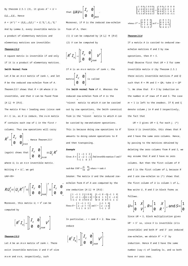
Example

Solution: The matrix U and the reduced roe-echelon form R of

A are computed by the row reduction [A I3] [R U]:

In particular, r = rank R = 2. Now row-reduce

[ RT I 4 ]→[ [I r 00 0]

nxm

V T ].

Theorem 2.5.4

If a matrix A is carried to reduced row-echelon matrices R and

S by row operations, then R = S.

Proof: Observe first that UR = S for some invertible matrix U

(by Theorem 2.5.1 there exists invertible matrices P and Q

such that R = PA and S = QA; take U = QP-1). We show that R

= S by induction on the number m of rows of R and S. The case

m = 1 is left to the readers. If Rj and Sj denote column j in R

and S respectively, the fact that

UR = S gives UR = Sj for each j. (*)

Since U is invertible, this shows that R and S have the same

zero columns. Hence, by passing to the matrices obtained by

deleting the zero columns from R and S, we may assume that R

and S have no zero columns. But then the first column of R

and S is the first column of Im because R and S are row-echelon

so (*) shows that the first column of U is column 1 of Im. Now

write U, R and S in block forms as follows.

U=[1 X0 V ] , R=[1 X

0 R ' ] ,and S=[1 Z0 S ' ]

Since UR = S, block multiplication gives VR’ = S’ so, since V

is invertible (U is invertible) and both R’ and S’ are reduced

row-echelon, we obtain R’ = S’ by induction. Hence R and S

have the same number (say r) of leading 1s, and so both have

m-r zero rows.

If fact, R and S have leading ones in the same columns, say r

of them. Applying (*) to these columns shows that the first r

columns of U are the first r columns of Im. Hence we can write

U, R and S in block form as follows:

U=[ I r M0 W ] , R=[R1 R2

0 0 ] , and S=[ S1 S2

0 0 ]where R1 and S1 are r x r. Then block multiplication gives UR

= R; that is, S = R. This completes the proof.

Linear Transformation

A transformationT : Rn→ Rm is called a linear

transformation if it satisfies the following two conditions for

all vectors x and y in Rn and all scalars a.

T1 T(x+y) = T(x) + T(y) T preserves addition

T2 T(ax) = aT(x) T preserves multiplication

Theorem 2.6.1

If T : Rn→ Rm is a linear transformation, then for each

k = 1, 2, …

T(a1x1 + a2x2 + … + akxk) = a1T(x1) + a2T(x2) + … + akT(xk)

For all scalars ai and all vectors xi in Rn

Standard basis

The standard basis of Rn is the set of columns {e1, e2, …, en}

of the identity matrix In. Then each ei is in Rn and every

vector x = [x1 x2 … xn]T in Rn is a linear combination of the ei.

x = x1e1 + x2e2 + … + xnen

Theorem 2.6.1 shows that

T(x) = T(x1e1 + x2e2 + … + xkek)

= x1T(e1) + x2T(e2) + … + xkT(ek)

Now observe that each T(ei) is a column in Rm, so

A = [T(e1) T(e2) … T(ek)] is an m x n matrix.

T(x) = x1T(e1) + x2T(e2) + … + xkT(ek)

= [T(e1) T(e2) … T(ek)] [x1 x2 … xn]T = Ax

Since this holds for every x in Rn, it shows that T is the

matrix transformation induced by A.

Theorem 2.6.2

Let T : Rn→ Rm be a transformation.

(1) T is linear if and only if it is a matrix transformation.

(2) In this case T = TA is the matrix transformation induced by

a unique m x n matrix A, given in terms of its columns by

A = [T(e1) T(e2) … T(ek)]

Where {e1, e2, …, en} is the standard basis of Rn.

Theorem 2.6.3

Let Rk T

→Rn S

→Rm, be linear transformations, and let A

and B

be the matrices of S and T respectively. Then S∘T is linear

with matrix AB.

Proof: S∘T (x) = S[T(x)] = A[Bx] = (AB)x for all x in Rk .

Some Geometry

It is convenient to view a vector x in R2 as an arrow from the

origin to the point x.

Scalar Multiple Law

Let x be a vector in R2. The arrow for kx is |k| times as long as

the arrow for x, and is in the same direction as the arrow for x

if k>0, and in the opposite direction if k<0.

Parallelogram Law

Consider vectors x and y in R2. If the arrows for x and y are

drawn, the arrow x+y corresponds to the fourth vertex of the

parallelogram determined by the points x, y and 0.

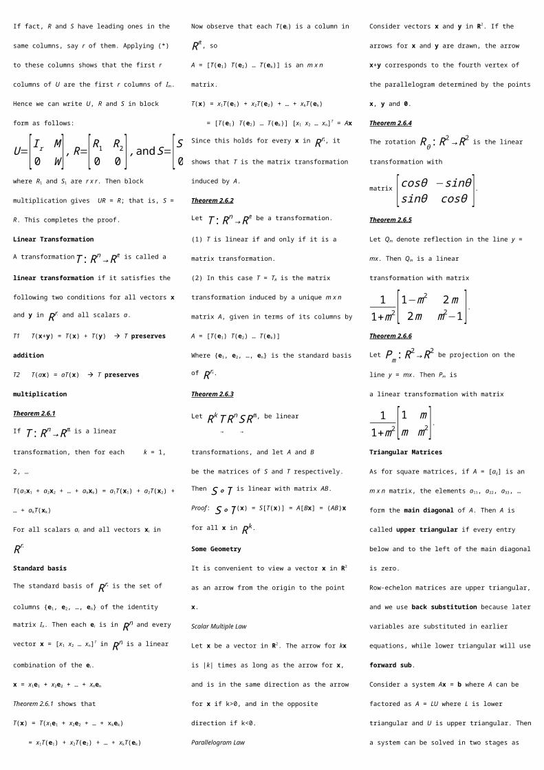
Theorem 2.6.4

The rotation Rθ : R2→ R2 is the linear transformation

with

matrix [cosθ −sinθsinθ cosθ ].

Theorem 2.6.5

Let Qm denote reflection in the line y = mx. Then Qm is a linear

transformation with matrix

11+m2 [1−m2 2m

2m m2−1].

Theorem 2.6.6

Let Pm : R2→ R2 be projection on the line y = mx. Then

Pm is

a linear transformation with matrix 1

1+m2 [ 1 mm m2].

Triangular Matrices

As for square matrices, if A = [aij] is an m x n matrix, the

elements a11, a22, a33, … form the main diagonal of A. Then A

is called upper triangular if every entry below and to the left

of the main diagonal is zero.

Row-echelon matrices are upper triangular, and we use back

substitution because later variables are substituted in earlier

equations, while lower triangular will use forward sub.

Consider a system Ax = b where A can be factored as A = LU

where L is lower triangular and U is upper triangular. Then a

system can be solved in two stages as follows:

(1) First solve Ly = b for y by forward substitution.

(2) Then solve Ux = y for x by back substitution.

Ax = LUx = Ly = b and take y = Ux.

Lemma: (1) If A and B are both lower (upper) triangular, the

same is true for AB. (2) If A is n x n and lower (upper)

triangular, then A is invertible if and only if every main

diagonal entry is nonzero. In this case A-1 is also lower (upper)

triangular.

LU-Factorization

Let A be an m x n matrix. Then A can be carried out to a row-

echelon matrix U (that is, upper triangular).

A E1A E2E1A E3E2E1A … EkEk-1…E2E1A = U

where E1, E2, …, Ek denote the corresponding elementary

matrices. Hence, A = LU,

where L = (EkEk-1…E2E1)-1 = E1-1E2

-1… Ek-1-1Ek

-1

If we do not insist that U is reduced then, except for row

interchanges, none of these row operations involve adding a

row to a row above it. Thus, if no row interchanges are used,

all the Ei are lower triangular, and so L is lower triangular (and

invertible by the lemma). A can be lower reduced if it can be

carried to row-echelon form using no row interchanges.

Theorem 2.7.1

If A can be lower reduced to a row-echelon matrix U, then

A = LU, where L is lower triangular and invertible and U is

upper triangular and row-echelon.

LU-Algorithm

The first nonzero column from the left in a matrix A is called

the leading column of A.

Let A be an m x n matrix with rank r, and suppose that A can

be lower reduced to a row-echelon matrix U. Then A = LU

where the lower triangular, invertible matrix L is constructed

as follows:

(1) If A = 0, take L = Im and U = 0

(2) If A ≠ 0, write A1 = A and let c1 be the leading column

of A1. Use c1 to create the first leading 1 and create zeros

below it (using the lower reduction). When this is completed,

let A2 denote the matrix consisting of rows 2 to m of the matrix

just created.

(3) If A2 ≠ 0, let c2 be the leading column of A2 and repeat

Step 2 on A2 to create A3.

(4) Continue in this way until U is reached, where all the rows

below the last leading 1 consists of zeros. This will happen

after r steps.

(5) Create L by replacing c1, c2, …, cr at the bottom of the first

r columns of Im.

Example

Find and LU-factorization for

A=[ 5−3−21

−532

−1

1020

10

02

−12

5105].

Solution

[ 5−3−21

−532

−1

1020

10

02

−12

5105]→[100

0

−1000

2848

02

−12

1424]→[100

0

−1000

2100

01/4−20

11/2

00

]→[1000

−1000

2100

01/410

11/2

00

]=U

.

If U denotes this row-echelon matrix, then A = LU, where

L=[ 5−3−21

0848

00

−20

0001].

Theorem 2.7.2

Suppose an m x n matrix A is carried to a row-echelon matrix

U via the Gaussian algorithm. Let P1, P2, …, Ps be the

elementary matrices corresponding (in order) to the row

interchanges used, and write P = Ps…P2P1. (If no interchanges

are used take P = Im) Then,

(1) PA is the matrix obtained from A by doing these

interchanges (in order) to A.

(2) PA has an LU-factorization.

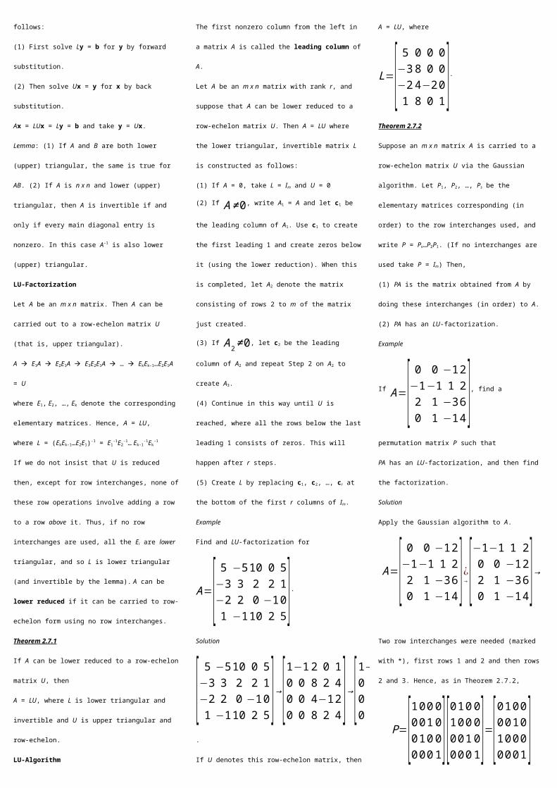
Example

If A=[ 0−120

0−111

−11

−3−1

2264], find a permutation matrix P

such that

PA has an LU-factorization, and then find the factorization.

Solution

Apply the Gaussian algorithm to A.

A=[ 0−120

0−111

−11

−3−1

2264] ¿→ [−1

020

−1011

1−1−3−1

2264]→

Two row interchanges were needed (marked with *), first rows

1 and 2 and then rows 2 and 3. Hence, as in Theorem 2.7.2,

P=[1000

0010

0100

0001][010

0

1000

0010

0001]=[001

0

1000

0100

0001]

If we do these interchanges (in order) to A, the result is PA.

Now apply the LU-algorithm to PA:

PA =

[−1200

−1101

1−3−1−1

2624]→[100

0

1−101

−1−1−1−1

−21024

]→[1000

1100

−11

−1−2

−2−10

214

]→[1000

1100

−1110

−2−10−210

]→[1000

1100

−1110

−2−10−21

]=U

.

Hence, PA = LU,

U=[1000

1100

−1110

−2−10−21

] , L=[−1−200

0−100

00

−1−2

000

10].

If A is any m x n matrix, it asserts that there exists a

permutation matrix P and an LU-factorization PA = LU.

Moreover, it shows that either P = I or P = Ps…P2P1, where

P1, P2, …, Ps are the elementary permutation matrices arising

in the reduction of A to row-echelon form. Now observe that

Pi-1 = Pi for each i (they are elementary row changes). Thus, P-1

= P1P2…Ps, so the matrix A can be factorized as

A = P-1LU where P-1 is the permutation matrix, L is lower

triangular and invertible, and U is a row-echelon matrix.

This is called a PLU-factorization of A.

Theorem 2.7.3

Let A be an m x n matrix that has an LU-factorization A = LU,

if A has rank m (that is, U has no rows of zeros), then L and U

are uniquely determined by A.

Lemma: Let Pk result from interchanging row k of Im with a

row below it. If j<k, let cj be a column of length m-j+1, Then

there is another column cj’ of length m-j+1 such that

Pk∙L(m)[k1, …, kj-1, cj] = L(m) [k1, …, kj-1, cj']∙Pk

Chapter 3 Determinants and Diagonalization

Cofactors

Assume that determinants of (n-1) x (n-1) matrices have been

defined. Given the n x n matrix A, let:

Aij denote the (n-1) x (n-1) matrix obtained from A by deleting

row i and column j.

Then, the (i,j)-cofactor cij(A) is the scalar defined by:

cij(A) = (-1)i+j det(Aij)

Here (-1)i+j is called the sign of the (i,j)-position.

Cofactor Expansion

Assume that determinants of (n-1) x (n-1) matrices have been

defined. If A = [aij] is n x n define

det A = a11c11(A) + a12c12(A) + … + a1nc1n(A)

Theorem 3.1.1

Cofactor Expansion Theorem

The determinant of an n x n matrix A can be computed by

using the cofactor expansion along any row or column if A.

That is det A can be computed by multiplying each entry of the

row or column by the corresponding cofactor and adding the

results.

Theorem 3.1.2

Let A denote an n x n matrix.

(1) If A has a row or column of zeros, det A = 0

(2) If two distinct rows (or columns) of A are interchange, the

determinant of the resulting matrix is –det A.

(3) If a row (or column) of A is multiplied by a constant u, the

determinant of the resulting matrix is u(det A).

(4) If two distinct rows (or columns) of A are identical, detA=0

(5) If a multiple of one row of A is added to a different row (or

if a multiple of a column is added to a different column), the

determinant of the resulting matrix is det A.

Theorem 3.1.3

If A is an n x n matrix, then det(uA) = undet A for any number u

Theorem 3.1.4

If A is a square triangular matrix, then det A is the product of

the entries on the main diagonal.

Theorem 3.1.5

Consider matrices [A X0 B ] and [A 0

Y B] in block

form, where

A and B are square matrices. Then

det[A X0 B ] = det A det B and det[A 0

Y B] = det A

det B.

Theorem 3.1.6

Given columns c1, …, cj-1, cj+1, …, cn in Rn, define T :

Rn → Rby

T(x) = det[c1 … cj-1 x cj+1 … cn] for all x in Rn.

Then, for all x and y in Rn and all a in R,

T(x + y) = T(x) + T(y) and T(ax) = aT(x)

Theorem 3.2.1

Product Theorem

If A and B are n x n matrices, then det(AB) = det A det B.

Theorem 3.2.2

An n x n matrix A is invertible if and only if det A≠ 0. When

this is the case, det(A-1) = (det A)-1

Theorem 3.2.3

If A is any square matrix, det AT = det A.

Orthogonal Matrix

A-1 = AT, det A = ±1

Adjugates

The adjugate of A, denoted as adj(A), is the transpose of this

cofactor matrix, is symbols, adj(A) = [cij(A)]T.

Theorem 3.2.4

Adjugates Formula

If A is any square matrix, then A(adj A) = (det A)I = (adj A)A.

In particular, if det A≠0, the inverse of A is given by

A-1 = (det A)-1 adj A

Theorem 3.2.5

Cramer’s Rule

If A is an invertible n x n matrix, the solution to the system Ax

= b of n equations in the variables x1, x2, …, xn is given by

x1=det A1

det A, x2=

det A2

det A, …, xn=

det An

det A

where, for each k, Ak is the matrix obtained from A by

replacing column k by b.

Theorem 3.2.6

Polynomial Interpolation

Let n data pairs (x1, y1), (x2, y2), …, (xn, yn) be given, and

assume that the xi are distinct. Then there exists a unique

polynomial p(x) = r0 + r1x + r2x2 + … + rn-1xn-1, such that p(xi)

= yi for each i = 1, 2, …, n.

Theorem 3.2.7

Vandermonde determinant

Let a1, a2, …, an be numbers where n≥2. Then the

corresponding Vandermonde determinant is given by

det [1 a1 a1

2

1 a2 a22

1 a3 a32

⋯a1

n−1

a2n−1

a3n−1

⋮ ⋱ ⋮1 an an

2 ⋯ ann−1

]= ∏1 ≤ j ≤i ≤n

(a i−a j)

For example, if n = 4, it is

(a4-a3) (a4-a2) (a4-a1) (a3-a2) (a3-a1) (a2-a1)

Theorem 3.3.1

If A = PDP-1 then Ak = PDkP-1 for k = 1, 2, …

Eigenvalues and Eigenvectors

If A is an n x n matrix, a number λ is called the eigenvalue of

A is Ax = λx for some column x≠0 in Rn.

In this case, x is called an eigenvector of A corresponding to

the eigenvalue λ , or a λ-eigenvector for short.

Characteristic Polynomial

If A is an n x n matrix, the characteristic polynomial cA(x) of

A is defined by cA(x) = det(xI - A)

Theorem 3.3.2

Let A be an n x n matrix,

(1) The eigenvalues λ of A are the roots of the characteristic

polynomial cA(x) of A.

(2) The λ-eigenvectors x are the nonzero solutions to the

homogeneous system (λI - A)x = 0

of linear equations with λI – A as coefficient matrix.