Math408: Combinatorics

University of North Dakota Mathematics Department

Spring 2011

Copyright (C) 2010,2011 University of North Dakota Mathematics Department. Permissionis granted to copy, distribute and/or modify this document under the terms of the GNUFree Documentation License, Version 1.3 or any later version published by the Free SoftwareFoundation; with no Invariant Sections, no Front-Cover Texts, and no Back-Cover Texts. Acopy of the license is included in the section entitled ”GNU Free Documentation License”.

Table of Contents

Chapter 0: Introduction . . . . . . . . . . . . . . . . . . . . . . . . . . . . . . . . . . . . . . . . . . . . . . . . . . . . . . . . . . . . . . . . . . 1Chapter 1: Basic Counting . . . . . . . . . . . . . . . . . . . . . . . . . . . . . . . . . . . . . . . . . . . . . . . . . . . . . . . . . . . . . . . .2

Section 1: Counting Principles . . . . . . . . . . . . . . . . . . . . . . . . . . . . . . . . . . . . . . . . . . . . . . . . . . . . . . . .2Section 2: Permutations and Combinations . . . . . . . . . . . . . . . . . . . . . . . . . . . . . . . . . . . . . . . . . . .3Section 3: Combinatorial Arguments and the Binomial Theorem . . . . . . . . . . . . . . . . . . . . . . 3Section 4: General Inclusion/Exclusion . . . . . . . . . . . . . . . . . . . . . . . . . . . . . . . . . . . . . . . . . . . . . . . 5Section 5: Novice Counting . . . . . . . . . . . . . . . . . . . . . . . . . . . . . . . . . . . . . . . . . . . . . . . . . . . . . . . . . . .7Section 6: Occupancy Problems . . . . . . . . . . . . . . . . . . . . . . . . . . . . . . . . . . . . . . . . . . . . . . . . . . . . . 10

Chapter 2: Introduction to Graphs . . . . . . . . . . . . . . . . . . . . . . . . . . . . . . . . . . . . . . . . . . . . . . . . . . . . . . .17Section 1: Graph Terminology . . . . . . . . . . . . . . . . . . . . . . . . . . . . . . . . . . . . . . . . . . . . . . . . . . . . . . .17Section 2: Graph Isomorphism . . . . . . . . . . . . . . . . . . . . . . . . . . . . . . . . . . . . . . . . . . . . . . . . . . . . . . 19Section 3: Paths . . . . . . . . . . . . . . . . . . . . . . . . . . . . . . . . . . . . . . . . . . . . . . . . . . . . . . . . . . . . . . . . . . . . 20Section 4: Trees . . . . . . . . . . . . . . . . . . . . . . . . . . . . . . . . . . . . . . . . . . . . . . . . . . . . . . . . . . . . . . . . . . . . . 23Section 5: Graph Coloring . . . . . . . . . . . . . . . . . . . . . . . . . . . . . . . . . . . . . . . . . . . . . . . . . . . . . . . . . . 24

Chapter 3: Intermediate Counting . . . . . . . . . . . . . . . . . . . . . . . . . . . . . . . . . . . . . . . . . . . . . . . . . . . . . . . 31Section 1: Generating Functions . . . . . . . . . . . . . . . . . . . . . . . . . . . . . . . . . . . . . . . . . . . . . . . . . . . . . 31Section 2: Applications to Counting . . . . . . . . . . . . . . . . . . . . . . . . . . . . . . . . . . . . . . . . . . . . . . . . . 32Section 3: Exponential Generating Functions . . . . . . . . . . . . . . . . . . . . . . . . . . . . . . . . . . . . . . . . 34Section 4: Recurrence Relations . . . . . . . . . . . . . . . . . . . . . . . . . . . . . . . . . . . . . . . . . . . . . . . . . . . . . 36Section 5: The Method of Characteristic Roots . . . . . . . . . . . . . . . . . . . . . . . . . . . . . . . . . . . . . 38Section 6: Solving Recurrence Relations by the Method of Generating Functions . . . . . 41

Chapter 4: PolyaCounting . . . . . . . . . . . . . . . . . . . . . . . . . . . . . . . . . . . . . . . . . . . . . . . . . . . . . . . . . . . . . . . 52Section 1: Equivalence Relations . . . . . . . . . . . . . . . . . . . . . . . . . . . . . . . . . . . . . . . . . . . . . . . . . . . . 52Section 2: Permutation Groups . . . . . . . . . . . . . . . . . . . . . . . . . . . . . . . . . . . . . . . . . . . . . . . . . . . . . . 53Section 3: Group Actions . . . . . . . . . . . . . . . . . . . . . . . . . . . . . . . . . . . . . . . . . . . . . . . . . . . . . . . . . . . .55Section 4: Colorings . . . . . . . . . . . . . . . . . . . . . . . . . . . . . . . . . . . . . . . . . . . . . . . . . . . . . . . . . . . . . . . . .57Section 5: The Cycle Index and the Pattern Inventory . . . . . . . . . . . . . . . . . . . . . . . . . . . . . . . 58

Chapter 5: Combinatorial Designs . . . . . . . . . . . . . . . . . . . . . . . . . . . . . . . . . . . . . . . . . . . . . . . . . . . . . . . 63Section 1: Finite Prime Fields . . . . . . . . . . . . . . . . . . . . . . . . . . . . . . . . . . . . . . . . . . . . . . . . . . . . . . . 63Section 2: Finite Fields . . . . . . . . . . . . . . . . . . . . . . . . . . . . . . . . . . . . . . . . . . . . . . . . . . . . . . . . . . . . . .67Section 3: Latin Squares . . . . . . . . . . . . . . . . . . . . . . . . . . . . . . . . . . . . . . . . . . . . . . . . . . . . . . . . . . . . 70Section 4: Introduction to Balanced Incomplete Block Designs . . . . . . . . . . . . . . . . . . . . . . . 74Section 5: Sufficient Conditions for, and Constructions of BIBDs . . . . . . . . . . . . . . . . . . . . . 77Section 6: Finite Plane Geometries . . . . . . . . . . . . . . . . . . . . . . . . . . . . . . . . . . . . . . . . . . . . . . . . . . 79

Chapter 6: Introductory Coding Theory . . . . . . . . . . . . . . . . . . . . . . . . . . . . . . . . . . . . . . . . . . . . . . . . . .83Section 1: Basic Background . . . . . . . . . . . . . . . . . . . . . . . . . . . . . . . . . . . . . . . . . . . . . . . . . . . . . . . . 83Section 2: Error Detection, Error Correction, and Distance . . . . . . . . . . . . . . . . . . . . . . . . . . 84Section 3: Linear Codes . . . . . . . . . . . . . . . . . . . . . . . . . . . . . . . . . . . . . . . . . . . . . . . . . . . . . . . . . . . . . 86

Appendices: . . . . . . . . . . . . . . . . . . . . . . . . . . . . . . . . . . . . . . . . . . . . . . . . . . . . . . . . . . . . . . . . . . . . . . . . . . . . 911: Polya’s Theorem and Structure in Cyclic Groups . . . . . . . . . . . . . . . . . . . . . . . . . . . . . . . . . .912: Some Linear Algebra . . . . . . . . . . . . . . . . . . . . . . . . . . . . . . . . . . . . . . . . . . . . . . . . . . . . . . . . . . . . 933: Some Handy Mathematica Commands . . . . . . . . . . . . . . . . . . . . . . . . . . . . . . . . . . . . . . . . . . . . 944. GNU Free Documentation License . . . . . . . . . . . . . . . . . . . . . . . . . . . . . . . . . . . . . . . . . . . . . . . 95

i

Chapter 0: Overview

There are three essential problems in combinatorics. These are the existence problem, thecounting problem, and the optimization problem. This course deals primarily with the first twoin reverse order.

The first two chapters are preparatory in nature. Chapter 1 deals with basic counting.Since Math208 is a prerequisite for this course, you should already have a pretty good grasp ofthis topic. This chapter will normally be covered at an accelerated rate. Chapter 2 is a shortintroduction to graph theory - which serves as a nice tie-in between the counting problem, andthe existence problem. Graph theory is also essential for the optimization problem. Not everyinstructor of Math208 covers graph theory beyond the basics of representing relations on aset via digraphs. This short chapter should level the playing field between those students whohave seen more graph theory and those who have not.

Chapter 3 is devoted to intermediate counting techniques. Again, some of this materialwill be review for certain, but not all, students who have successfully completed Math208. Thematerial on generating functions requires some ability to manipulate power series in a formalfashion. This explains why Calculus II is a prerequisite for this course.

Counting theory is crowned by the so-called Polya Counting, which is the topic of Chapter4. Polya Counting requires some basic group theory. This is not the last topic where abstractalgebra rears its head.

The terminal chapters are devoted to combinatorial designs and a short introduction tocoding theory. The existence problem is the main question addressed here. The flavor ofthese notes is to approach the problems from an algebraic perspective. Thus we will spendconsiderable effort investigating finite fields and finite geometries over finite fields.

My personal experience was that seeing these algebraic structures in action before takingabstract algebra was a huge advantage. I’ve also encountered quite a few students who tookthis course after completing abstract algebra. Prior experience with abstract algebra did notnecessarily give them an advantage in this course, but they did tend to come away with amuch improved opinion of, and improved respect for, the field of abstract algebra.

1

Chapter 1: Basic Counting

We generally denote sets by capital English letters, and their elements as lowercase Englishletters. We denote the cardinality of a finite set, A, by |A|. A set with |A| = n is called ann-set. We denote an arbitrary universal set by U , and the complement of a set (relative to U)by A. Unless otherwise indicated, all sets mentioned in this chapter are finite sets.

§1.1 Counting Principles

The basic principles of counting theory are the multiplication principle, the principle ofinclusion/exclusion, the addition principle, and the exclusion principle.

The multiplication principle states that the cardinality of a Cartesian product is the prod-uct of the cardinalities. In the most basic case we have |A× B| = |A| · |B|. An argument forthis is that A × B consists of all ordered pairs (a, b) where a ∈ A and b ∈ B. There are |A|choices for a and then |B| choices for b. A common rephrasing of the principle is that if a taskcan be decomposed into two sequential subtasks, where there are n1 ways to complete the firstsubtask, and then n2 ways to complete the second subtask, then altogether there are n1 · n2

ways to complete the task.Notice the connection between the multiplication principle and the logical connective

AND. Also, realize that this naturally extends to general Cartesian products with finitelymany terms.

Example: The number of binary strings of length 10 is 210 since it is |{0, 1}|10.

Example: The number of ternary strings of length n is 3n.

Example: The number of functions from a k-set to an n-set is nk.

Example: The number of strings of length k using n symbols with repetition allowed is nk.

Example: The number of 1-1 functions from a k-set to an n-set is n·(n−1)·(n−2)·...·(n−(k−1)).

The basic principle of inclusion/exclusion states that |A∪B| = |A|+ |B|− |A∩B|. So weinclude elements when either in A, or in B, but then have to exclude the elements in A ∩ B,since they’ve been included twice each.

Example: How many students are there in a discrete math class if 15 students are computerscience majors, 7 are math majors, and 3 are double majors in math and computer science?

Solution: Let A denote the subset of computer science majors in the class, and B denotethe math majors. Then |A| = 15, |B| = 7 and |A ∩ B| = 3 = 0. So by the principle ofinclusion/exclusion there are 15 + 7− 3 = 19 students in the class.

The general principle of inclusion/exclusion will be discussed in a later section.

The addition principle is a special case of the principle of inclusion/exclusion. If A∩B = ∅,then |A ∪ B| = |A| + |B|. In general the cardinality of a finite collection of pairwise disjointfinite sets is the sum of their cardinalities. That is, if Ai ∩Aj = ∅ for i = j, and |Ai| <∞ for

all i, then

∣∣∣∣ n∪i=1

Ai

∣∣∣∣ = n∑i=1

|Ai|.

The exclusion principle is a special case of the addition principle. A set and its complementare always disjoint, so |A|+ |A| = |U|, or equivalently |A| = |U| − |A|.

2

§1.2 Permutations and Combinations

Given an n-set of objects, an r-string from the n-set is a sequence of length r. We takethe convention that the string is identified with its output list. So the string a1 = a, a2 =b, a3 = c, a4 = b is denoted abcb.

The number of r-strings from a set of size n is nr as we saw in the previous section. As astring we see that order matters. That is, the string abcd is not the same as the string bcad.Also repetition is allowed, since for example aaa is a 3-string from the set of lowercase Englishletters.

An r-permutation from an n-set is an ordered selection of r distinct objects from the n-set.We denote the number of r-permutations of an n-set P (n, r). By the multiplication principle

P (n, r) = n(n− 1) · ... · (n− (r − 1)) = n(n− 1) · ... · (n− r + 1) =n!

(n− r)!.

The number P (n, r) is the same as the number of one-to-one functions from a set of sizer to a set of size n.

An r-combination from an n-set is an unordered collection of r distinct elements fromthe set. In other words an r-combination of an n-set is a r-subset. We denote the number of

r-combinations from an n-set by C(n, r) or

(n

r

).

Theorem 1 r!

(n

r

)= P (n, r)

Proof: For each r-combination from an n-set, there are r! ways for us to order the set withoutrepetition. Each ordering gives rise to exactly one r-permutation from the n-set. Every r-permutation from the n-set arises in this fashion.

Corollary 1

(n

r

)=

n!

r!(n− r)!

Since n− (n− r) = r, we also have

Corollary 2

(n

r

)=

(n

n− r

)Example: Suppose we have a club with 20 members. If we want to select a committee of 5members, then there are C(20, 5) ways to do this since the order of people on the committeedoesn’t matter. However if the club wants to elect a board of officers consisting of a president,vice president, secretary, treasurer, and sergeant-at-arms, then there are P (20, 5) ways to dothis. In each instance, repetition is not allowed. What makes the difference between the twocases is that the first is an unordered selection without repetition, whereas the second is anordered selection without repetition.

§1.3 Combinatorial Arguments and the Binomial Theorem

One of the most famous combinatorial arguments is attributed to Blaise Pascal and bears

his name. The understanding we adopt is that any number of the form

(m

s

), where m and s

are integers, is zero, if either s > m, or s < 0 (or both).

3

Theorem (Pascal’s Identity) Let n and k be non-negative integers, then

(n+ 1

k

)=

(n

k − 1

)+

(n

k

)

Proof: Let S be a set with n + 1 elements, and let a ∈ S. Put T = S − {a} so |T | = n. On

the one hand S has

(n+ 1

k

)subsets of size k. On the other hand, S has

(n

k

)k-subsets which

are subsets of T and

(n

k − 1

)k-subsets consisting of a together with a (k − 1)-subset of T .

Since these two types of subsets are disjoint, the result follows by the addition principle.

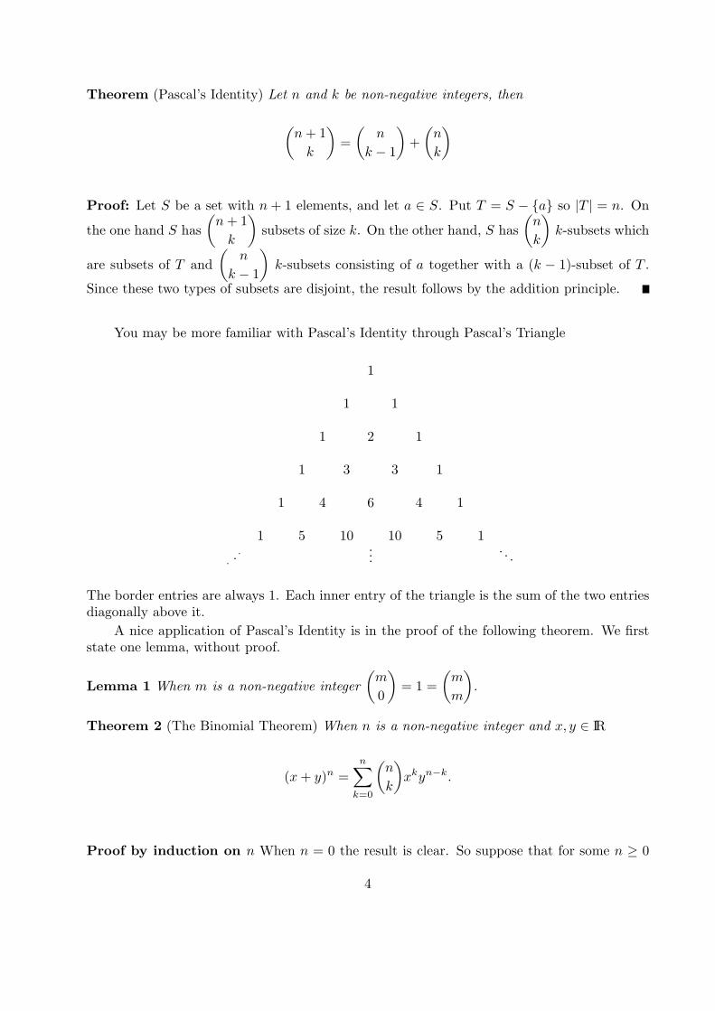
You may be more familiar with Pascal’s Identity through Pascal’s Triangle

1

1 1

1 2 1

1 3 3 1

1 4 6 4 1

1 5 10 10 5 1

. ··...

. . .

The border entries are always 1. Each inner entry of the triangle is the sum of the two entriesdiagonally above it.

A nice application of Pascal’s Identity is in the proof of the following theorem. We firststate one lemma, without proof.

Lemma 1 When m is a non-negative integer

(m

0

)= 1 =

(m

m

).

Theorem 2 (The Binomial Theorem) When n is a non-negative integer and x, y ∈ IR

(x+ y)n =n∑

k=0

(n

k

)xkyn−k.

Proof by induction on n When n = 0 the result is clear. So suppose that for some n ≥ 0

4

we have (x+ y)n =n∑

k=0

(n

k

)xkyn−k, for any x, y ∈ IR. Then

(x+ y)n+1 = (x+ y)n(x+ y), by recursive definition of integral exponents

=[ n∑k=0

(n

k

)xkyn−k

](x+ y), by inductive hypothesis

=[ n∑k=0

(n

k

)xk+1yn−k

]+[ n∑k=0

(n

k

)xkyn+1−k

]=

(n

n

)xn+1 +

[ n−1∑k=0

(n

k

)xk+1yn−k

]+[ n∑k=1

(n

k

)xkyn+1−k

]+

(n

0

)yn+1

=

(n

n

)xn+1 +

[ n∑l=1

(n

l − 1

)xlyn−(l−1)

]+[ n∑k=1

(n

k

)xkyn+1−k

]+

(n

0

)yn+1

=

(n

n

)xn+1 +

[ n∑l=1

(n

l − 1

)xlyn+1−l

]+[ n∑k=1

(n

k

)xkyn+1−k

]+

(n

0

)yn+1

=

(n

n

)xn+1 +

[ n∑k=1

[( n

k − 1

)+

(n

k

)]xkyn+1−k

]+

(n

0

)yn+1

=

(n+ 1

n+ 1

)xn+1 +

[ n∑k=1

(n+ 1

k

)xkyn+1−k

]+

(n+ 1

0

)yn+1,by Pascal′s identity

=n+1∑k=0

(n+ 1

k

)xkyn+1−k

From the binomial theorem we can derive facts such as

Theorem 3 A finite set with n elements has 2n subsets

Proof: By the addition principle the number of subsets of an n-set is

n∑k=0

(n

k

)=

n∑k=0

(n

k

)1k1n−k.

By the binomial theoremn∑

k=0

(n

k

)1k1n−k = (1 + 1)n = 2n

§1.4 General Inclusion/Exclusion

In general when we are given n finite sets A1, A2, ..., An and we want to compute thecardinality of their generalized union we use the following theorem.

5

Theorem 1 Given finite sets A1, A2, ..., An∣∣∣ n∪k=1

Ak

∣∣∣ = [ n∑k=1

|Ak|]−[ ∑1≤j<k≤n

|Aj∩Ak|]+[ ∑1≤i<j<k≤n

|Ai∩Aj∩Ak|]+...+(−1)n+1

∣∣∣ n∩k=1

Ak

∣∣∣Proof: We draw this as a corollary of the next theorem.

Let U be a finite universal set which contains the general union of A1, A2, ..., An. Tocompute the cardinality of the general intersection of complements of A1, A2, ..., An we use thegeneral version of DeMorgan’s laws and the principle of exclusion. That is

∣∣∣ n∩k=1

Ak

∣∣∣ = |U| − ∣∣∣ n∩k=1

Ak

∣∣∣ = |U| − ∣∣∣ n∪k=1

Ak

∣∣∣.So equivalent to theorem 1 is

Theorem 2 Given finite sets A1, A2, ..., An∣∣∣ n∩k=1

Ak

∣∣∣ = |U| − [ n∑k=1

|Ak|]+[ ∑1≤j<k≤n

|Aj ∩Ak|]− ...+ (−1)n

∣∣∣ n∩k=1

Ak

∣∣∣Proof: Let x ∈ U . Then two cases to consider are 1) x ∈ Ai for all i and 2) x ∈ Ai for exactlyp of the sets Ai, where 1 ≤ p ≤ n.

In the first case, x is counted once on the left hand side. It is also counted only once onthe right hand side in the |U| term. It is not counted in any of the subsequent terms on theright hand side.

In the second case, x is not counted on the left hand side, since it is not in the generalintersection of the complements.

Denote the term |U| as the 0th term,n∑

k=1

|Ak| as the 1st term, etc. Since x is a member

of exactly p of the sets A1, ..., An, it gets counted

(p

m

)times in the mth term. (Remember

that

(n

k

)= 0, when k > n)

So the total number of times x is counted on the right hand side is(p

0

)−(p

1

)+

(p

2

)− ...+ (−1)p

(p

p

).

All terms of the form

(p

k

), where k > p do not contribute. By the binomial theorem

0 = 0p = (1 + (−1))p =

(p

0

)−(p

1

)+

(p

2

)− ...+ (−1)p

(p

p

).

6

So the count is correct.

Example 1 How many students are in a calculus class if 14 are math majors, 22 are computerscience majors, 15 are engineering majors, and 13 are chemistry majors, if 5 students aredouble majoring in math and computer science, 3 students are double majoring in chemistryand engineering, 10 are double majoring in computer science and engineering, 4 are doublemajoring in chemistry and computer science, none are double majoring in math and engineeringand none are double majoring in math and chemistry, and no student has more than twomajors?

Solution: Let A1 denote the math majors, A2 denote the computer science majors, A3 denotethe engineering majors, and A4 the chemistry majors. Then the information given is|A1| = 14, |A2| = 22, |A3| = 15, |A4| = 13, |A1 ∩A2| = 5, |A1 ∩A3| = 0, |A1 ∩A4| = 0,|A2 ∩A3| = 10, |A2 ∩A4| = 4, |A3 ∩A4| = 3, |A1 ∩A2 ∩A3| = 0, |A1 ∩A2 ∩A4| = 0|A1 ∩A3 ∩A4| = 0, |A2 ∩A3 ∩A4| = 0, |A1 ∩A2 ∩A3 ∩A4| = 0.

So by the general rule of inclusion/exclusion, the number of students in the class is 14 +22 + 15 + 13− 5− 10− 4− 3 = 32.

Example 2 How many ternary strings (using 0’s, 1’s and 2’s) of length 8 either start with a 1,end with two 0’s or have 4th and 5th positions 12?

Solution: Let A1 denote the set of ternary strings of length 8 which start with a 1, A2 denote theset of ternary strings of length 8 which end with two 0’s, and A3 denote the set of ternary stringsof length 8 which have 4th and 5th positions 12. By the general rule of inclusion/exclusionour answer is

37 + 36 + 36 − 35 − 35 − 34 + 33

§1.5 Novice Counting

All of the counting exercises you’ve been asked to complete so far have not been realistic.In general it won’t be true that a counting problem fits neatly into a section. So we need towork on the bigger picture.

When we start any counting exercise it is true that there is an underlying exercise at thebasic level that we want to consider first. So instead of answering the question immediately wemight first want to decide on what type of exercise we have. So far we have seen three typeswhich are distinguishable by the answers to two questions.

1) In forming the objects we want to count, is repetition or replacement allowed?

2) In forming the objects we want to count, does the order of selection matter?

The three scenarios we have seen so far are described in the table below.

Order Repetition Type FormY Y r-strings nr

Y N r-permutations P (n, r)N N r-combinations

(nr

)There are two problems to address. First of all the table above is incomplete. What about,

for example, counting objects where repetition is allowed, but order doesn’t matter. Second

7

of all, there are connections among the types which make some solutions appear misleading.But as a general rule of thumb, if we correctly identify the type of problem we are workingon, then all we have to do is use the principles of addition, multiplication, inclusion/exclusion,or exclusion to decompose our problem into subproblems. The solutions to the subproblemsoften have the same form as the underlying problem. The principles we employed direct us onhow the sub-solutions should be recombined to give the final answer.

As an example of the second problem, if we ask how many binary strings of length 10contain exactly three 1’s, then the underlying problem is an r-string problem. But in this case

the answer is

(10

3

). Of course this is really

(10

3

)1317 from the binomial theorem. In this case

the part of the answer which looks like nr is suppressed since it’s trivial. To see the differencewe might ask how many ternary strings of length 10 contain exactly three 1’s. Now the answer

is

(10

3

)1327, since we choose the three positions for the 1’s to go in, and then fill in each of

the 7 remaining positions with a 0 or a 2.

To begin to address the first problem we introduce

The Donut Shop Problem If you get to the donut shop before the cops get there, you will findthat they have a nice variety of donuts. You might want to order several dozen. They willput your order in a box. You don’t particularly care what order the donuts are put into thebox. You do usually want more than one of several types. The number of ways for you tocomplete your order is therefore a counting problem where order doesn’t matter, and repetitionis allowed.

In order to answer the question of how many ways you can complete your order, wefirst recast the problem mathematically. From among n types of objects we want to select robjects. If xi denotes the number of objects of the ith type selected, we have 0 ≤ xi, (since wecannot choose a negative number of chocolate donouts), also xi ∈ ZZ, (since we cannot selectfractional parts of donuts). So the different ways to order are in one-to-one correspondencewith the solutions in non-negative integers to x1 + x2 + ...+ xn = r.

Next, in order to compute the number of solutions in non-negative integers to x1 + x2 +...+xn = r, we model each solution as a string (possibly empty) of x1 1’s followed by a +, thena string of x2 1’s followed by a +, ... then a string of xn−1 1’s followed by a +, then a string ofxn 1’s. So for example, if x1 = 2, x2 = 0, x3 = 1, x4 = 3 is a solution to x1 + x2 + x3 + x4 = 6the string we get is 11++1+111. So the total number of solutions in non-negative integers tox1 + ...+ xn = r, is the number of binary strings of length r + n− 1 with exactly r 1’s. From

the remark above, this is

(n+ r − 1

r

).

The donut shop problem is not very realistic in two ways. First it is common that someof your order will be determined by other people. You might for example canvas the peoplein your office before you go to see if there is anything you can pick up for them. So whereasyou want to order r donuts, you might have been asked to pick up a certain number of varioustypes.

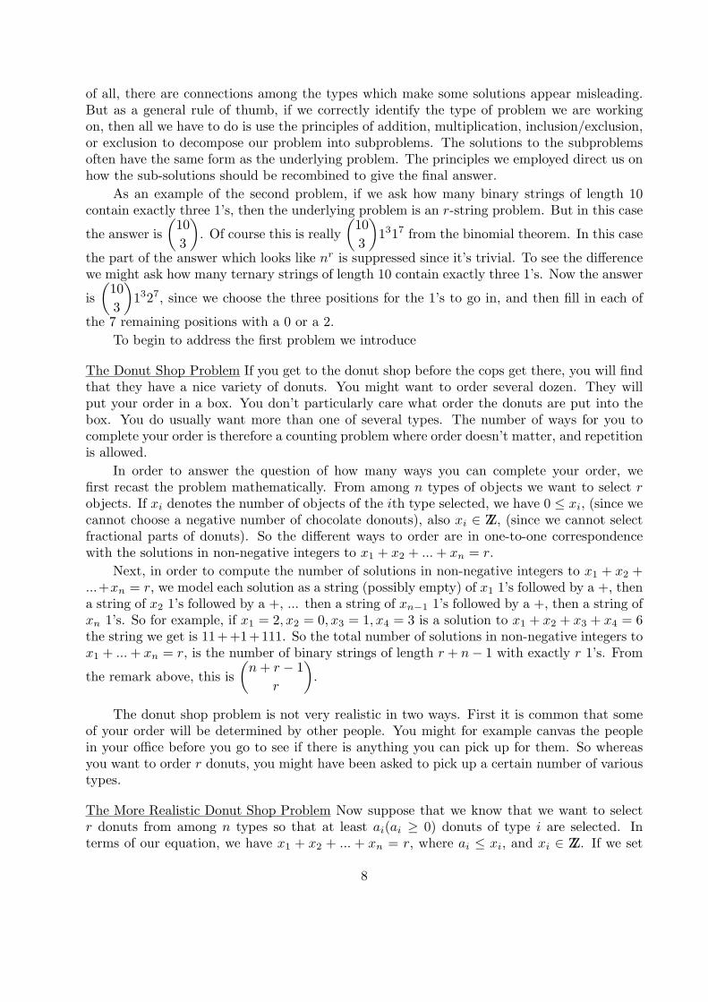
The More Realistic Donut Shop Problem Now suppose that we know that we want to selectr donuts from among n types so that at least ai(ai ≥ 0) donuts of type i are selected. Interms of our equation, we have x1 + x2 + ... + xn = r, where ai ≤ xi, and xi ∈ ZZ. If we set

8

yi = xi − ai for i = 1, ..., n, and a =n∑

i=1

ai, then 0 ≤ yi, yi ∈ ZZ and

n∑i=1

yi =

n∑i=1

(xi − ai) = [

n∑i=1

xi]− [

n∑i=1

ai] = r − a

So the number of ways to complete our order is

(n+ (r − a)− 1

(r − a)

).

Still, we qualified the donut shop problem by supposing that we arrived before the copsdid.

The Real Donut Shop Problem If we arrive at the donut shop after canvassing our friends, wewant to select r donuts from among n types. The problem is that there are probably only afew left of each type. This may place an upper limit on how often we can select a particulartype. So now we wish to count solutions to ai ≤ xi ≤ bi, xi ∈ ZZ, and x1+x2+ ...+xn = r. Weproceed by replacing r by s = r−a, where a is the sum of lower bounds. We also replace bi byci = bi − ai for i = 1, ..., n. So we want to find the number of solutions to 0 ≤ yi ≤ ci, yi ∈ ZZ,and y1 + y2 + ...+ yn = s. There are several ways to proceed. We choose inclusion/exclusion.Let us set U to be all solutions in non-negative integers to y1+ ...+yn = s. Next let Ai denotethose solutions in non-negative integers to y1 + ... + yn = r, where ci < yi. Then we want tocompute |A1 ∩ A2 ∩ A3 ∩ ... ∩ An|, which we can do by general inclusion/exclusion, and theideas from the more realistic donut shop problem.

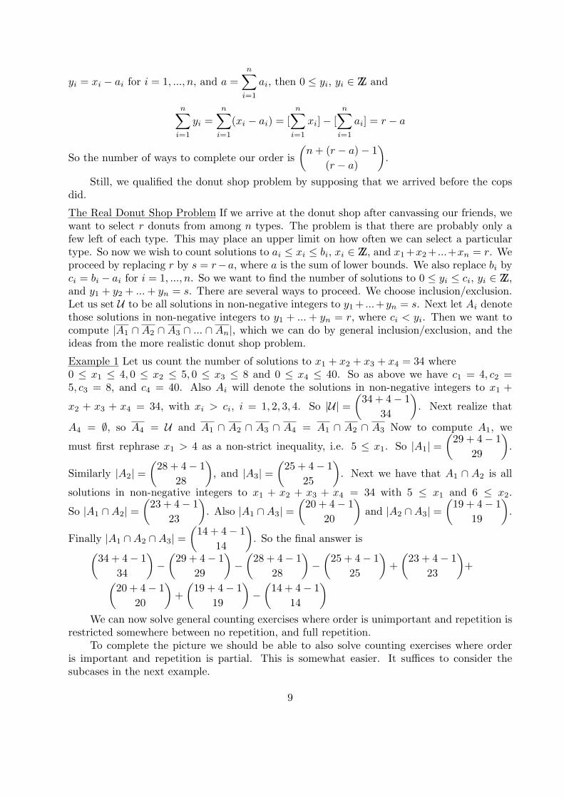
Example 1 Let us count the number of solutions to x1 + x2 + x3 + x4 = 34 where0 ≤ x1 ≤ 4, 0 ≤ x2 ≤ 5, 0 ≤ x3 ≤ 8 and 0 ≤ x4 ≤ 40. So as above we have c1 = 4, c2 =5, c3 = 8, and c4 = 40. Also Ai will denote the solutions in non-negative integers to x1 +

x2 + x3 + x4 = 34, with xi > ci, i = 1, 2, 3, 4. So |U| =(34 + 4− 1

34

). Next realize that

A4 = ∅, so A4 = U and A1 ∩ A2 ∩ A3 ∩ A4 = A1 ∩ A2 ∩ A3 Now to compute A1, we

must first rephrase x1 > 4 as a non-strict inequality, i.e. 5 ≤ x1. So |A1| =(29 + 4− 1

29

).

Similarly |A2| =(28 + 4− 1

28

), and |A3| =

(25 + 4− 1

25

). Next we have that A1 ∩ A2 is all

solutions in non-negative integers to x1 + x2 + x3 + x4 = 34 with 5 ≤ x1 and 6 ≤ x2.

So |A1 ∩A2| =(23 + 4− 1

23

). Also |A1 ∩A3| =

(20 + 4− 1

20

)and |A2 ∩A3| =

(19 + 4− 1

19

).

Finally |A1 ∩A2 ∩A3| =(14 + 4− 1

14

). So the final answer is(

34 + 4− 1

34

)−

(29 + 4− 1

29

)−(28 + 4− 1

28

)−(25 + 4− 1

25

)+

(23 + 4− 1

23

)+(

20 + 4− 1

20

)+

(19 + 4− 1

19

)−(14 + 4− 1

14

)We can now solve general counting exercises where order is unimportant and repetition is

restricted somewhere between no repetition, and full repetition.To complete the picture we should be able to also solve counting exercises where order

is important and repetition is partial. This is somewhat easier. It suffices to consider thesubcases in the next example.

9

Example 2 Let us take as initial problem the number of quaternary strings of length 15. There

are 415 of these. Now if we ask how many contain exactly two 0’s, the answer is

(15

2

)313. If

we ask how many contain exactly two 0’s and four 1’s, the answer is

(15

2

)(13

4

)29. And if we

ask how many contain exactly two 0’s, four 1’s and five 2’s, the answer is

(15

2

)(13

4

)(9

5

)(4

4

).

So in fact many types of counting are related by what we call the multinomial theorem.

Theorem 1 When r is a non-negative integer and x1, x2, ..., xn ∈ IR

(x1 + x2 + ...+ xn)r =

∑e1+e2+...+en=r

0≤ei

(r

e1, e2, ...en

)xe11 xe2

2 ...xenn ,

where

(r

e1, e2, ...en

)=

r!

e1!e2!...en!.

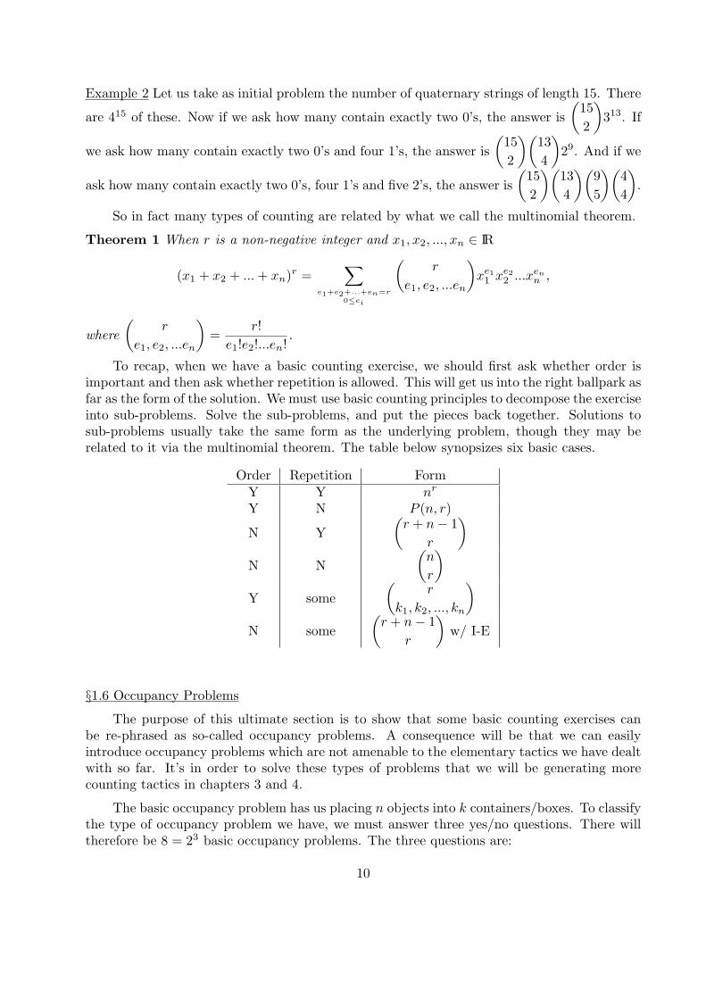
To recap, when we have a basic counting exercise, we should first ask whether order isimportant and then ask whether repetition is allowed. This will get us into the right ballpark asfar as the form of the solution. We must use basic counting principles to decompose the exerciseinto sub-problems. Solve the sub-problems, and put the pieces back together. Solutions tosub-problems usually take the same form as the underlying problem, though they may berelated to it via the multinomial theorem. The table below synopsizes six basic cases.

Order Repetition FormY Y nr

Y N P (n, r)

N Y

(r + n− 1

r

)N N

(n

r

)Y some

(r

k1, k2, ..., kn

)N some

(r + n− 1

r

)w/ I-E

§1.6 Occupancy Problems

The purpose of this ultimate section is to show that some basic counting exercises canbe re-phrased as so-called occupancy problems. A consequence will be that we can easilyintroduce occupancy problems which are not amenable to the elementary tactics we have dealtwith so far. It’s in order to solve these types of problems that we will be generating morecounting tactics in chapters 3 and 4.

The basic occupancy problem has us placing n objects into k containers/boxes. To classifythe type of occupancy problem we have, we must answer three yes/no questions. There willtherefore be 8 = 23 basic occupancy problems. The three questions are:

10

1) Are the objects distinguishable from one another?2) Are the boxes distinguishable from one another?3) Can a box remain unoccupied?

If the answer to all three questions is yes, then the number of ways to place the n objectsinto the k boxes is clearly the number of functions from an n-set to a k-set, which is kn.

If, on the other hand the answer to the first question is no, but the other two answersare yes, then we have the basic donut shoppe problem. So the number of ways to distributen identical objects among k distinguishable boxes is the number of solutions in non-negativewhole numbers to x1 + x2 + ...+ xk = n, where xi is the number of objects placed in the ithbox.

If we change the answer to the third question to no, then we have the more realistic donutshoppe problem. Now we need the number of solutions in positive integers to x1+ ...+xk = n,or equivalently the number of solutions in non-negative integers to y1 + ...+ yk = n− k. Thisis C((n− k) + k − 1, n− k) = C(n− 1, n− k) = C(n− 1, k − 1).

So it might appear that there is nothing really new here. That every one of our occupancyproblems can be solved by an elementary counting technique. However if we define S(n, k) tobe the number of ways to distribute n distinguishable objects into k indistinguishable boxeswe will derive in chapter 3 that

S(n, k) =1

k!

k∑i=0

(−1)i(k

i

)(k − i)n.

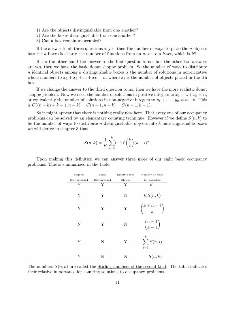
Upon making this definition we can answer three more of our eight basic occupancyproblems. This is summarized in the table.

Objects Boxes Empty boxes Number of ways

Distinguished Distingushed allowed to complete

Y Y Y kn

Y Y N k!S(n, k)

N Y Y

(k + n− 1

k

)

N Y N

(n− 1

k − 1

)

Y N Yk∑

i=1

S(n, i)

Y N N S(n, k)

The numbers S(n, k) are called the Stirling numbers of the second kind. The table indicatestheir relative importance for counting solutions to occupancy problems.

11

We close this section by pointing out that two occupancy problems remain. A partitionof a positive integer n is a collection of positive integers which sum to n.

Example: The partitions of 5 are {5}, {4, 1}, {3, 2}, {3, 1, 1}, {2, 2, 1}, {2, 1, 1, 1}, {1, 1, 1, 1, 1}.

So the number of ways to place n indistinguishable objects into k indistinguishable boxesif no box is empty is the number of partitions of n into exactly k parts. If we denote thisby pk(n), then we see that p2(5) = 2. Also p1(n) = pn(n) = 1 for all positive integers n.Meanwhile pk(n) = 0 is k > n. Finally p2(n) = ⌈(n− 1)/2⌉.

The final occupancy problem is to place n indistinguishable objects into k indistinguishable

boxes if some boxes may be empty. The number of ways this can be done isk∑

i=1

pi(n). This is

the number of partitions of n into k or fewer parts.A more complete discussion of the partitions of integers into parts can be found in most

decent number theory books, or a good combinatorics reference book like Marshall Hall’s.

12

Chapter 1 Exercises

1. How many non-negative whole numbers less than 1 million contain the digit 2?

2. How many bit strings have length 3, 4 or 5?

3. How many whole numbers are there which have five digits, each being a number in{1, 2, 3, 4, 5, 6, 7, 8, 9}, and either having all digits odd or having all digits even?

4. How many 5-letter words from the lowercase English alphabet either start with f or do nothave the letter f?

5. In how many ways can we get a sum of 3 or a sum of 4 when two dice are rolled?

6. List all permutations of {1, 2, 3}. Repeat for {1, 2, 3, 4}.

7. How many permutations of {1, 2, 3, 4, 5} begin with 5?

8. How many permutations of {1, 2, 3, ...., n} begin with 1 and end with n?

9. Find a) P (3, 2), b) P (5, 3), c) P (8, 5), d) P (1, 3).

10. Let A = {0, 1, 2, 3, 4, 5, 6}.a) Find the number of strings of length 4 using elements of A.

b) Repeat part a, if no element of A can be used twice.

c) Repeat part a, if the first element of the string is 3

d) Repeat part c, if no element of A can be used twice.

11. Enumerate the subsets of {a, b, c, d}.

12. If A is a 9-set, how many nonemepty subsets does A have?

13. If A is an 8-set, how many subsets with more than 2 elements does A have?

14. Find a) C(6, 3), b) C(7, 4), c) C(n, 1), d) C(2, 5).

15. In how many ways can 8 blood samples be divided into 2 groups to be sent to differentlaboratories for testing, if there are four samples per group.

16. Repeat exercise 15, if the laboratories are not distinguishable.

17. A committee is to be chosen from a set of 8 women and 6 men. How many ways are thereto form the committee if

a) the committee has 5 people, 3 women and 2 men?

b) the committee has any size, but there are an equal number of men and women?

c) the committee has 7 people and there must be more men than women?

18. Prove that

(n

m

)(m

k

)=

(n

k

)(n− k

m− k

).

19. Give a combinatorial argument to prove Vandermonde’s identity(n+m

r

)=

(n

0

)(m

r

)+

(n

1

)(m

r − 1

)+ ...+

(n

k

)(m

r − k

)+ ...+

(n

r

)(m

0

)13

20. Prove that

(n

0

)+

(n+ 1

1

)+

(n+ 2

2

)+ ...+

(n+ r

r

)=

(n+ r + 1

r

).

21. Calculate the probabilty that when a fair 6-sided die is tossed, the outcome is

a) an odd number.

b) a number less than or equal to 2.

c) a number divisible by 3,

22. Calculate the probability that in 4 tosses of a fair coin, there are at most 3 heads.

23. Calculate the probability that a family with three children has

a) exactly 2 boys.

b) at least 2 boys.

c) at least 1 boy and at least 1 girl.

24. What is the probability that a bit string of length 5, chosen at random, does not have twoconsecutive zeroes?

25. Suppose that a system with four independent components, each of which is equally likelyto work or to not work. Suppose that the system works if and only if at least three componentswork. What is the probability that the system works?

26. In how many ways can we choose 8 bottles of soda if there are 5 brands to choose from?

27. Find all partitions of a) 4, b) 6, c) 7.

28. Find all partitions of 8 into four or fewer parts.

29. Compute a) S(n, 0), b) S(n, 1), c) S(n, 2), d) S(n, n− 1), e) S(n, n)

30. Show by a combinatorial argument that S(n, k) = kS(n− 1, k) + S(n− 1, k − 1).

31. How many solutions in non-negative integers are there to x1 + x2 + x3 + x4 = 18 whichsatisfy 1 ≤ xi ≤ 8 for i = 1, 2, 3, 4?

32. Expand a) (x+ y)5, b) (a+ 2b)3, c) (2u+ 3v)4

33. Find the coefficient of x11 in the expansion of

a) (1 + x)15, b) (2 + x)13, c) (2x+ 3y)11

34. What is the coefficient of x10 in the expansion of (1 + x)12(1 + x)4?

35. What is the coefficient of a3b2c in the expansion of (a+ b+ c+ 2)8?

36. How many solutions in non-negative integers are there to x1 + x2 + x3 + x4 + x5 = 47which satisfy x1 ≤ 6, x2 ≤ 8, and x3 ≤ 10?

37. Findn∑

k=0

2k(n

k

).

38. Findn∑

k=0

4k(n

k

).

14

39.n∑

k=0

xk

(n

k

).

40. An octapeptide is a chain of 8 amino acids, each of which is one of 20 naturally occurringamino acids. How many octapeptides are there?

41. In an RNA chain of 15 bases, there are 4 A’s, 6 U’s, 4 G’s, and 1 C. If the chain beginswith AU and ends with UG, how many chains are there?

42. An ice cream parlor offers 29 different flavors. How many different triple cones are possibleif each scoop on the cone has to be a different flavor?

43. A cigarette company surveys 100,000 people. Of these 40,000 are males, according to thecompany’s report. Also 80,000 are smokers and 10,000 of those surveyed have cancer. However,of those suveyed, there are 1000 males with cancer, 2000 smokers with cancer, and 3000 malesmokers. Finally there are 100 male smokers with cancer. How many female nonsmokerswithout cancer are there? Is there something wrong with the company’s report?

44. One hundred water samples were tested for traces of three different types of chemicals,mercury, arsenic, and lead. Of the 100 samples 7 were found to have mercury, 5 to have arsenic,4 to have lead, 3 to have mercury and arsenic, 3 to have arsenic and lead, 2 to have mercuryand lead, and 1 to have mercury, arsenic, but no lead. How many samples had a trace of atleast one of the three chemiclas?

45. Of 100 cars tested at an inspection station, 9 had defective headlights, 8 defective brakes,7 defective horns, 2 defective windshield wipers, 4 defective headlights and brakes, 3 defectiveheadlights and horns, 2 defective headlights and windshield wipers, 1 defective horn and wind-shield wipers, 1 had defective headlights, brakes and horn, 1 had defective headlights, horn,and windshield wipers, and none had any other combination of defects. Find the number ofcars which had at least one of the defects in question.

46. How many integers between 1 and 10,000 inclusive are divisible by none of 5, 7, and 11?

47. A multiple choice test contains 10 questions. There are four possible answers for eachquestion.a) How many ways can a student answer the questions if every question must be answered?b) How many ways can a student answer the questions if questions can be left unanswered?

48. How many positive integers between 100 and 999 inclusive are divisible by 10 or 25?

49. How many strings of eight lowercase English letters are there

a) if the letters may be repeated?

b) if no letter may be repeated?

c) which start with the letter x, and letters may be repeated?

d) which contain the letter x, and the letters may be repeated?

e) which contain the letter x, if no letter can be repeated?

f) which contain at least one vowel (a, e, i, o or u), if letters may be repeated?

g) which contain exactly two vowels, if letters may be repeated?

h) which contain at least one vowel, where letters may not be repeated?

15

50. How many bit strings of length 9 either begin “00”, or end “1010”?

51. In how many different orders can six runners finish a race if no ties occur?

52. How many subsets with an odd number of elements does a set with 10 elements have?

53. How many bit strings of length 9 have

a) exactly three 1’s?

b) at least three 1’s?

c) at most three 1’s?

d) more zeroes than ones?

54. How many bit strings of length ten contain at least three ones and at least three zeroes?

55. How many ways are there to seat six people around a circular table where seatings areconsidered to be equivalent if they can be obtained from each other by rotating the table?

56. Show that if n is a positive integer, then

(2n

2

)= 2

(n

2

)+ n2

a) using a combinatorial argument.

b) by algebraic manipulation.

57. How many bit strings of length 15 start with the string 101, end with the string 1001 orhave 3rd through 6 bits 1010?

58. How many positive integers between 1000 and 9999 inclusive are not divisible by any of4, 10 and 25?

59. How many quaternary strings of length n are there (a quaternary string uses 0’s, 1’s, 2’s,and 3’s)?

60. How many solutions in integers are there to x1+x2+x3+x4+x5+x6 = 54, where 3 ≤ x1,4 ≤ x2, 5 ≤ x3, and 6 < x4, x5, x6?

61. How many strings of twelve lowercase English letters are there

a) which start with the letter x, if letters may be repeated?

b) which contain the letter x, if letters can be repeated?

c) which contain the letters x and y, if letters can be repeated?

d) which contain at least one vowel, where letters may not be repeated?

62. How many bit strings of length 19 either begin “00”, or have 4th, 5th and 6th digits “101”,or end “1010”?

63. How many pentary strings of length 15 consist of two 0’s, four 1’s, three 2’s, five 3’s andone 4?

64. How many ternary strings of length 9 have

a) exactly three 1’s?

b) at least three 1’s?

c) at most three 1’s?

16

Chapter 2: Introduction to Graphs

You should already have some experience representing set-theoretic objects as digraphs.In this chapter we introduce some ideas and uses of undirected graphs, those whose edges arenot directed.

§2.1 Graph Terminology

Loosely speaking, an undirected graph is a doodle, where we have a set of points (calledvertices). Some of the points are connected by arcs (called edges). If our graph containsloops, we call it a pseudograph. If we allow multiple connections between vertices we have amultigraph. Clearly in order to understand pseudographs and multigraphs it will be necessaryto understand the simplest case, where we do not have multiple edges, directed edges, orloops. Such an undirected graph is called a simple graph if we need to distinguish it from apseudograph or a multigraph. Henceforth in this chapter, unless specified otherwise, graphmeans undirected, simple graph.

Formally a graph, G = (V,E) consists of a set of vertices V and a set E of edges, whereany edge e ∈ E corresponds to an unordered pair of vertices {u, v}. We say that the edge e isincident with u and v. The vertices u and v are adjacent, when {u, v} ∈ E. otherwise they arenot. We often write u ∼ v to denote that u and v are adjacent. We also call u and v neighborsin this case. Of course u ∼ v denotes that {u, v} ∈ E. All of our graphs will have finite vertexsets, and therefore finite edge sets.

Most often we won’t want to deal with the set-theoretic version of a graph, we will wantto work with a graphical representation, or a 0, 1-matrix representation. This presents aproblem since there is possibly more than one way of representing the graph either way. Wewill deal with this problem formally in the next section. To represent a graph graphically wedraw a point for each vertex, and use arcs to connect those points corresponding to adjacentvertices. To represent a graph as a 0, 1-matrix we can either use an adjacency matrix or anincidence matrix. In the first case we use the vertex set in some order to label rows and columns(same order) of a |V | × |V | matrix. The entry in the row labeled u and column labeled v is 1if u ∼ v and 0 if u ∼ v. In the second case we use V to index the rows of a |V | × |E| matrix,and E to index the columns. The entry in the row labeled u and column labeled e is 1 if u isincident with e, and 0 otherwise.

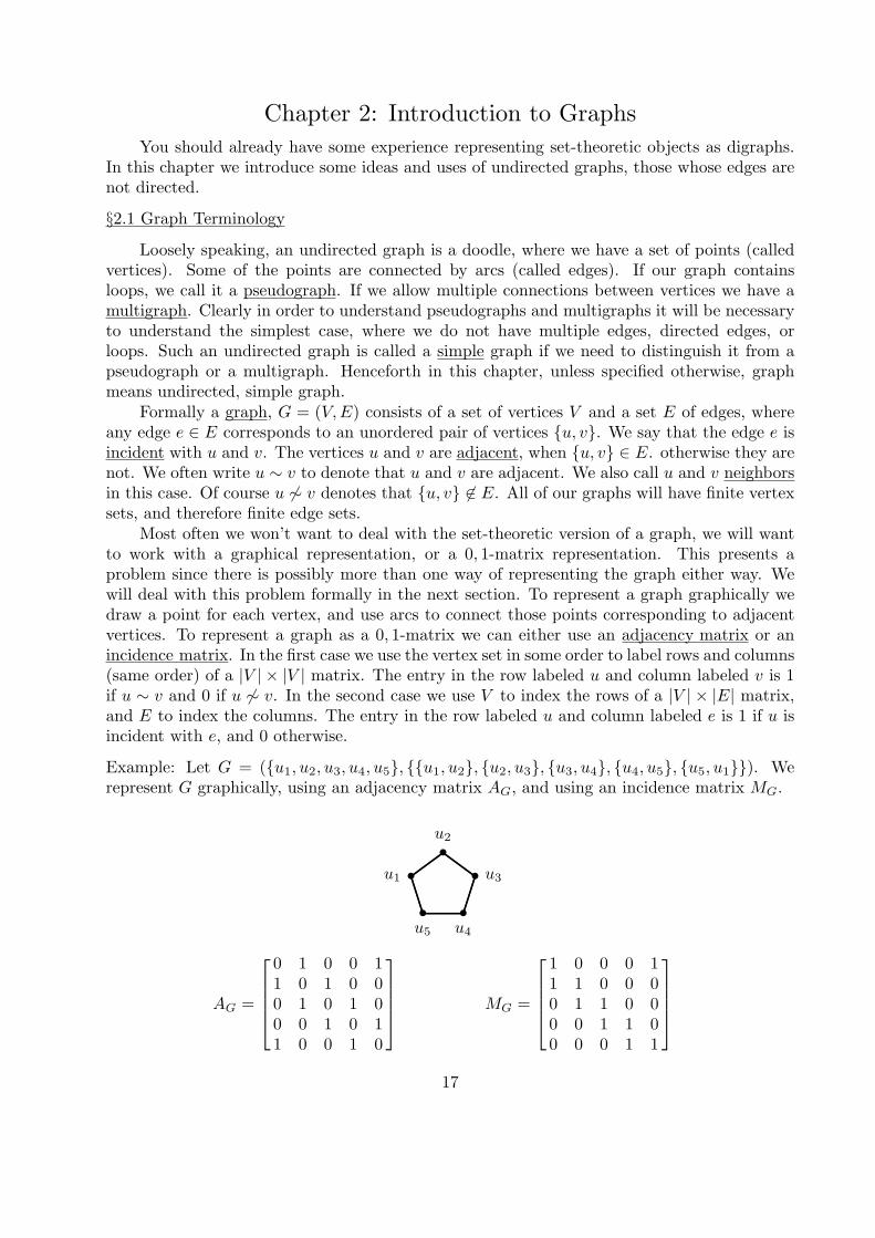
Example: Let G = ({u1, u2, u3, u4, u5}, {{u1, u2}, {u2, u3}, {u3, u4}, {u4, u5}, {u5, u1}}). Werepresent G graphically, using an adjacency matrix AG, and using an incidence matrix MG.

u2

u1 u3

u4u5

•••

••

...................................................................................................................................................................................

..........................................................

............................................................

AG =

0 1 0 0 11 0 1 0 00 1 0 1 00 0 1 0 11 0 0 1 0

MG =

1 0 0 0 11 1 0 0 00 1 1 0 00 0 1 1 00 0 0 1 1

17

All of these represent the same object. When doing graph theory we usually think of thegraphic object.

Now that we know what graphs are, we are naturally interested in their behavior. Forexample, for a vertex v in a graph G = (V,E) we denote the number of edges incident withv as deg(v), the degree of v. For a digraph it would then make sense to define the in-degreeof a vertex as the number of edges into v, and similarly the out-degree. These are denoted byid(v) and od(v) respectively.

Theorem (Hand-Shaking Theorem) In any graph G = (V,E),∑v∈V

deg(v) = 2|E|.

Proof: Every edge is incident with two vertices (counting multiplicity for loops).

Corollary In an undirected graph there are an even number of vertices of odd degree.

Corollary In a digraph D,∑v∈V

id(v) =∑v∈V

od(v) = |E|.

In order to explore the more general situations it is handy to have notation to describecertain special graphs. The reader is strongly encouraged to represent these graphically.

1) For n ≥ 0, Kn denotes the simple graph on n vertices where every pair of vertices is adjacent.K0 is of course the empty graph. Kn is the complete graph on n vertices.

2) For n ≥ 3, Cn denotes the simple graph on n vertices, v1, ..., vn, whereE = {{vi, vj}|j − i ≡ ±1 (mod n)}. Cn is the n-cycle.

3) For n ≥ 2, Ln denotes the n-link. L2 = K2, and for n > 2 Ln is the result of removing anyedge from Cn.

4) For n ≥ 3, Wn denotes the n-wheel. To form Wn add one vertex to Cn and make it adjacentto every other vertex.

5) For n ≥ 0, the n-cube, Qn, is the graph whose vertices are all binary strings of length n.Two vertices are adjacent only if they differ in exactly one position.

6) A graph is bipartite if there is a partition V = V1 ∪V2 so that any edge is incident with onevertex from each part of the partition. In case every vertex of V1 is adjacent to every vertexof V2 and |V1| = m with |V2| = n, the result is the complete bipartite graph Km,n.

As you might guess from the constructions of Ln and Wn from Cn it makes sense todiscuss the union and intersection of graphs. For a simple graph on n vertices, G, it evenmakes sense to discuss the complement G (relative to Kn).

As far as subgraphs are concerned we stress that a subgraph H = (W,F ) of a graphG = (V,E), has W ⊆ V , F ⊆ E, and if f = {u, v} ∈ F , then both u and v are in W . Finallywe define the induced subgraph on a subset W of V to be the graph with vertex set W , andall edges f = {u, v} ∈ E, where u, v ∈W .

18

§2.2 Graph Isomorphism

In this section we deal with the problem that there is more than one way to present a graph.Informally two graphs G = (V,E) and H = (W,F ) are isomorphic, if one can be redrawn to beidentical to the other. Thus the two graphs would represent equivalent set-theoretic objects.Clearly it is necessary that |V | = |W | and |E| = |F |.

Formally graphs G = (V,E) and H = (W,F ) are isomorphic if there exists a bijectivefunction φ : V −→ W , called a graph isomorphism, with the property that {u, v} ∈ E iff{φ(u), φ(v)} ∈ F . We write G ∼= H in case such a function exists. G ∼= H signifies that G andH are not isomorphic.

The property in the definition is called the adjacency-preserving property. It is absolutelyessential since for example L4 and K1,3 are both graphs with 4 vertices and 3 edges, yetthey are not isomorphic. In fact the adjacency-preserving property of a graph isomorphismguarantees that deg(u) = deg(φ(u)) for all u ∈ V . In particular if G ∼= H and the degrees ofthe vertices of G are listed in increasing order, then this list must be identical to the sequenceformed when the degrees of the vertices of H are listed in increasing order. The list of degreesof a graph, G, in increasing order is its degree sequence, and is denoted ds(G). Thus G ∼= Himplies ds(G) = ds(H). Equivalently ds(G) = ds(H) implies G ∼= H.

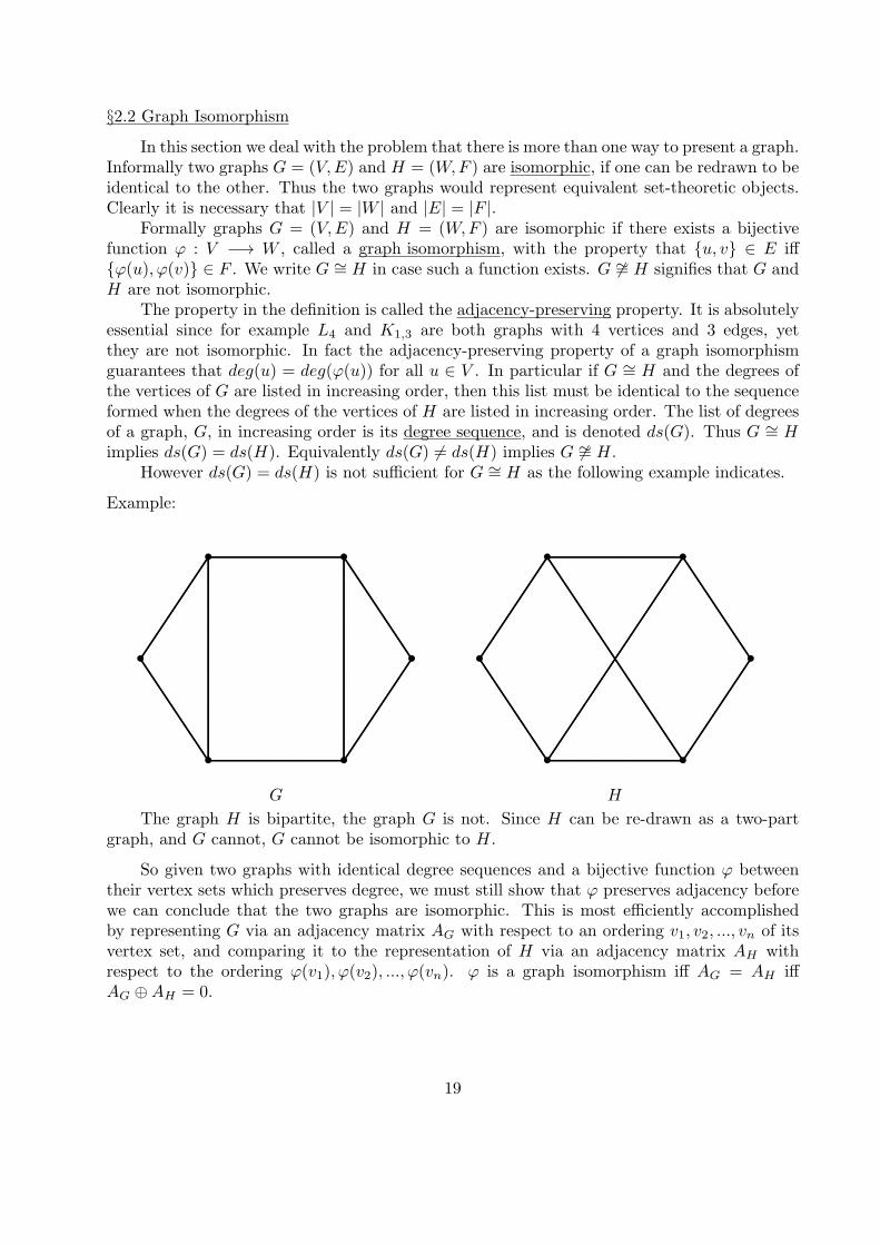
However ds(G) = ds(H) is not sufficient for G ∼= H as the following example indicates.

Example:

G H

• • • •

• • • •

• • • •

......................................................................................................................................................................................................... .........................................................................................................................................................................................................

.....................................................................................................................................................................................

.....................................................................................................................................................................................

......................................................................................................................................................................................................................................................................................................................................................................................................................................................................................................................

.............................................................................................................................................................................................................................................................................................................

.....................................................................................................................................................................................

..................................................................................................................................................................................... ................

.....................................................................................................................................................................

.....................................................................................................................................................................................

.........................................................................................................................................................................................................................................................................................................................................................................

..................................................................................................................................................................................................................................................................................................................................................................................................................................................................................................................................................................................

.....................................................................................................................................................................................

.....................................................................................................................................................................................

The graph H is bipartite, the graph G is not. Since H can be re-drawn as a two-partgraph, and G cannot, G cannot be isomorphic to H.

So given two graphs with identical degree sequences and a bijective function φ betweentheir vertex sets which preserves degree, we must still show that φ preserves adjacency beforewe can conclude that the two graphs are isomorphic. This is most efficiently accomplishedby representing G via an adjacency matrix AG with respect to an ordering v1, v2, ..., vn of itsvertex set, and comparing it to the representation of H via an adjacency matrix AH withrespect to the ordering φ(v1), φ(v2), ..., φ(vn). φ is a graph isomorphism iff AG = AH iffAG ⊕AH = 0.

19

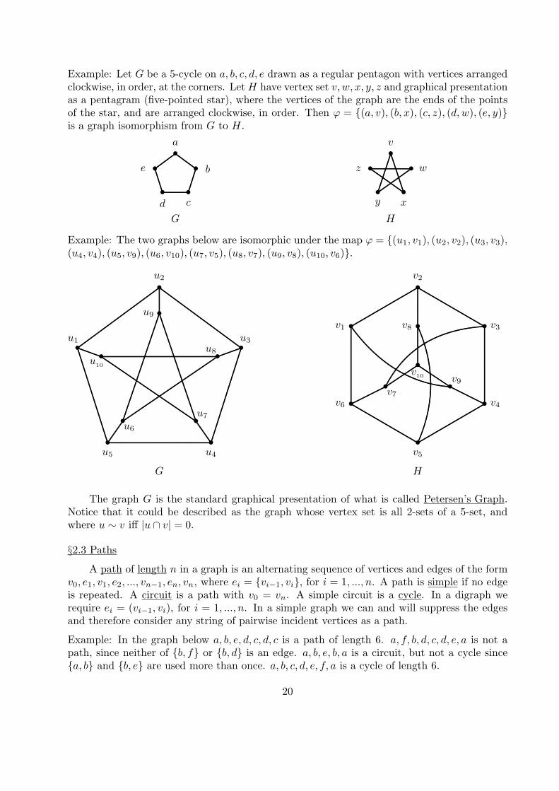
Example: Let G be a 5-cycle on a, b, c, d, e drawn as a regular pentagon with vertices arrangedclockwise, in order, at the corners. LetH have vertex set v, w, x, y, z and graphical presentationas a pentagram (five-pointed star), where the vertices of the graph are the ends of the pointsof the star, and are arranged clockwise, in order. Then φ = {(a, v), (b, x), (c, z), (d,w), (e, y)}is a graph isomorphism from G to H.

G

a

b

cd

e

•••

••

...................................................................................................................................................................................

..........................................................

............................................................

H

v

w

xy

z

•••

••

...............................................................................................

...............................................................................................................................................................................................................................................................................................................................................................................................

Example: The two graphs below are isomorphic under the map φ = {(u1, v1), (u2, v2), (u3, v3),(u4, v4), (u5, v9), (u6, v10), (u7, v5), (u8, v7), (u9, v8), (u10, v6)}.

u1

u2

u3

u4u5

u6

u7

u8

u9

u10

v1

v2

v3

v4

v5

v6v7

v8

v9v10

G H

•

•

• •• •

• •

• •

.............................................................

.............................................................................................................................................................................................................................................

.............................................................................................................................................................................................................................................

.........................................................................................................................................................................................................................................................................

.........................................................................................................................................................................................................................................................................

...........................................................

.......................................................................................................................................................................................................................................

..........................................................................................................................................................................................................................................................................................................................................................................................................................................................................................................................................................

..............................................................

...........................................................

...........................................................................................................................................................................................................................................................................

.................................................................................................................................................................................................................................................

.....................................................................................................................................................................................................................................................................................................

...........................................................................................

...............................................................................................................................................................................................................................................................................

....................................................................................................................................................................................

.........................................................................................................................................................................................................................................................................................................................................................................

........................................................

.............................................................................................................................

....................................................................................................................................................................................

.....................................................................................................................................................................................

.....................................................................................................................................................................................

•

•

•

•

• •

• •• •

....................................................................................................................................................................................................................................................................................... ............................................................................................................................................................................................................................................................................................

.......................................................................................................................................................................................................................................................................................

The graph G is the standard graphical presentation of what is called Petersen’s Graph.Notice that it could be described as the graph whose vertex set is all 2-sets of a 5-set, andwhere u ∼ v iff |u ∩ v| = 0.

§2.3 Paths

A path of length n in a graph is an alternating sequence of vertices and edges of the formv0, e1, v1, e2, ..., vn−1, en, vn, where ei = {vi−1, vi}, for i = 1, ..., n. A path is simple if no edgeis repeated. A circuit is a path with v0 = vn. A simple circuit is a cycle. In a digraph werequire ei = (vi−1, vi), for i = 1, ..., n. In a simple graph we can and will suppress the edgesand therefore consider any string of pairwise incident vertices as a path.

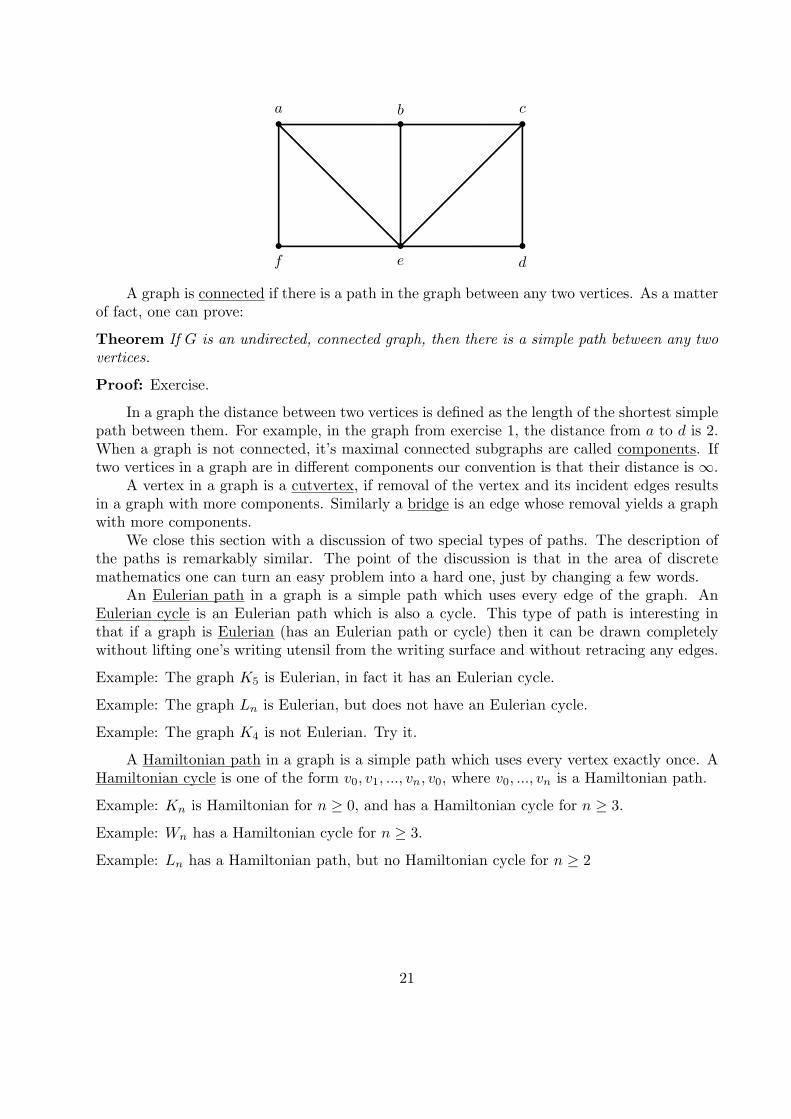
Example: In the graph below a, b, e, d, c, d, c is a path of length 6. a, f, b, d, c, d, e, a is not apath, since neither of {b, f} or {b, d} is an edge. a, b, e, b, a is a circuit, but not a cycle since{a, b} and {b, e} are used more than once. a, b, c, d, e, f, a is a cycle of length 6.

20

a b c

f e d

• • •

• • •

.................................................................................................................................................................................................................................................................................................................................................................................................................

.................................................................................................................................................................................................................................................................................................................................................................................................................

.........................................................................................................................................................................................................

.........................................................................................................................................................................................................

.........................................................................................................................................................................................................

......................................................................................................................................................................................................................................................................................................................................................................................................................................................................................................................................................................................

A graph is connected if there is a path in the graph between any two vertices. As a matterof fact, one can prove:

Theorem If G is an undirected, connected graph, then there is a simple path between any twovertices.

Proof: Exercise.

In a graph the distance between two vertices is defined as the length of the shortest simplepath between them. For example, in the graph from exercise 1, the distance from a to d is 2.When a graph is not connected, it’s maximal connected subgraphs are called components. Iftwo vertices in a graph are in different components our convention is that their distance is ∞.

A vertex in a graph is a cutvertex, if removal of the vertex and its incident edges resultsin a graph with more components. Similarly a bridge is an edge whose removal yields a graphwith more components.

We close this section with a discussion of two special types of paths. The description ofthe paths is remarkably similar. The point of the discussion is that in the area of discretemathematics one can turn an easy problem into a hard one, just by changing a few words.

An Eulerian path in a graph is a simple path which uses every edge of the graph. AnEulerian cycle is an Eulerian path which is also a cycle. This type of path is interesting inthat if a graph is Eulerian (has an Eulerian path or cycle) then it can be drawn completelywithout lifting one’s writing utensil from the writing surface and without retracing any edges.

Example: The graph K5 is Eulerian, in fact it has an Eulerian cycle.

Example: The graph Ln is Eulerian, but does not have an Eulerian cycle.

Example: The graph K4 is not Eulerian. Try it.

A Hamiltonian path in a graph is a simple path which uses every vertex exactly once. AHamiltonian cycle is one of the form v0, v1, ..., vn, v0, where v0, ..., vn is a Hamiltonian path.

Example: Kn is Hamiltonian for n ≥ 0, and has a Hamiltonian cycle for n ≥ 3.

Example: Wn has a Hamiltonian cycle for n ≥ 3.

Example: Ln has a Hamiltonian path, but no Hamiltonian cycle for n ≥ 2

21

These two types of path are similar, in that there is a list of necessary conditions whicha graph must satisfy, if it is to possess either type of cycle. If G is a graph with either anEulerian or Hamiltonian cycle, then

1) G is connected.2) every vertex has degree at least 2.3) G has no bridges.4) If G has a Hamiltonian cycle, then G has no cutvertices.These types of path are different in that Leonhard Euler completely solved the problem

of which graphs are Eulerian. Moreover the criteria is surprising simple. In contrast, no onehas been able to find a similar solution for the problem of which graphs are Hamiltonian.

Spurred by the Sunday afternoon pastime of people in Kaliningrad, Russia Euler provedthe following theorem.

Theorem A connected multigraph has an Eulerian cycle iff every vertex has even degree.

Proof: Let G be a connected multigraph with an Eulerian cycle and suppose that v is a vertexin G with deg(v) = 2m + 1, for some m ∈ IN. Let i denote the number of times the cyclepasses through v. Since every edge is used exactly once in the cycle, and each time v is visited2 different edges are used, we have 2i = 2m+ 1 −→←−.

Conversely, let G be a connected multigraph where every vertex has even degree. Selecta vertex u and build a simple path P starting at u. Each time a vertex is reached we add anyedge not already used. Any time a vertex v = u is reached its even degree guarantees a newedge out, since we used one edge to arrive there. Since G is finite, we must reach a vertexwhere P cannot continue. And this vertex must be u by the preceding remark. Therefore Pis a cycle.

If this cycle contains every edge we are done. Otherwise when these edges are removedfrom G we obtain a set of connected components H1, ..., Hm which are subgraphs of G andwhich each satisfy that all vertices have even degree. Since their sizes are smaller, we mayinductively construct an Eulerian cycle for each Hi. Since each G is connected, each Hi

contains a vertex of the initial cycle, say vj . If we call the Eulerian cycle of Hi, Ci, thenv0, ...vj , Ci, vj , ..., vn, v0 is a cycle in G. Since the Hi are disjoint, we may insert each Euleriansubcycle thus obtaining an Eulerian cycle for G.

As a corollary we have

Theorem A connected multigraph has an Eulerian path, but no Eulerian cycle iff it has exactlytwo vertices of odd degree.

The following theorem is an example of a sufficient condition for a graph to have a Hamil-tonian cycle. This condition is clearly not necessary by considering Cn for n ≥ 5.

Theorem Let G be a connected, simple graph on n ≥ 3 vertices. If deg(v) ≥ n/2 for everyvertex v, then G has a Hamiltonian cycle.

Proof: Suppose that the theorem is false. Let G satisfy the conditions on vertex degree,connectivity, and simplicity. Moreover suppose that of all counterexamples on n vertices, G ismaximal with respect to the number of edges.

G is not complete, since Kn has a Hamiltonian cycle, for n ≥ 3. Therefore G has twovertices v1 and vn with v1 ∼ vn. By maximality the graph G1 = G∪{v1, vn} has a Hamiltoniancycle. Moreover this cycle uses the edge {v1, vn}, else G has a Hamiltonian cycle. So we may

22

suppose that the Hamiltonian cycle in G1 is of the form v1, v2, ..., vn, v1. Thus v1, ..., vn is aHamiltonian path in G.

Let k = deg(v1). So k = |S| = |{v ∈ V |v1 ∼ v}|. If vi+1 ∈ S, then vi ∼ vn, elsev1, ..., vi, vn, vn−1, ..., vi+1, v1 is a Hamiltonian cycle in G. Therefore

deg(vn) ≤ (n− 1)− k ≤ n− 1− n/2 = n/2− 1. −→←−

§2.4 Trees

Trees are one of the most important classes of graphs. A tree is a connected, undirectedgraph, with no cycles. Consequently a tree is a simple graph. Moreover we have

Theorem A graph G is a tree iff there is a unique simple path between any two vertices.

Proof: Suppose that G is a tree, and let u and v be two vertices of G. Since G is connected,there is a simple path P of the form u = v0, v1, ..., vn = v. If Q is a different simple pathfrom u to v, say u = w0, w1, ..., wn = v let i be the smallest subscript so that wi = vi, butvi+1 = wi+1. Also let j be the next smallest subscript where vj = wj . By constructionvi, vi+1, ..., vj , wj−1, wj−2, ..., wi is a cycle in G −→←−.

Conversely, if G is a graph where there is a unique simple path between any pair ofvertices, then by definition G is connected. If G contained a cycle, C, then any two verticesof C would be joined by two distinct simple paths.−→←− Therefore G contains no cycles, andis a tree.

A consequence of theorem 1 is that given any vertex r in a tree, we can draw T with rat the top and the other vertices in levels below. The neighbors of r thus appear at the firstlevel and are called r’s children. The neighbors of r’s children are put in the second level, andare r’s grandchildren. In general the ith level consists of those vertices in the tree which areat distance i from r. The result is called a rooted tree. A rooted tree is by default directed,but we suppress the arrows on edges since every edge is drawn downwards. The height of arooted tree is the maximum level number.

Naturally, besides child and parent, many geneological terms apply to rooted trees, andare suggestive of the structure. For example if T = (V,E, r) is a rooted tree with root r,and v ∈ V − {r}, the ancestors of v are all vertices on the path from r to v, including r, butexcluding v. The descendants of a vertex, w consist of all vertices which have w as one of theirancestors. The subtree rooted at w is the rooted tree consisting of w, its descendants, and allrequisite paths. A vertex with no children is a leaf, and a vertex with at least one child iscalled an internal vertex.

To distinguish rooted trees by breadth, we use the term m-ary to mean that any internalvertex has at most m children. An m-ary tree is full if every internal vertex has exactly mchildren. When m = 2, we use the term binary.

As an initial application of rooted trees we prove the following theorem.

Theorem A tree on n vertices has n− 1 edges.

Proof: Let T = (V,E) be a tree with n vertices. Let u ∈ V and form the rooted treeT = (V,E, u) rooted at u. Any edge e ∈ E joins two vertices v and w where v is theparent of w. This allows us to define a function f : E −→ V − {u} by f(e) = w. f is

23

one-to-one by uniqueness of simple path from u to w. f is onto by connectivity. Therefore|E| = |V − {u}| = |V | − 1 = n− 1.

We draw as corollary

Corollary A full m-ary tree with i internal vertices has n = mi+ 1 vertices.

Since every vertex in a rooted tree is either internal or a leaf, we know that a full m-arytree with i internal vertices has l = (m − 1)i + 1 leaves. In short, if we know any two of thethree quantities n, i and l for a full m-ary tree, we can deduce the third.

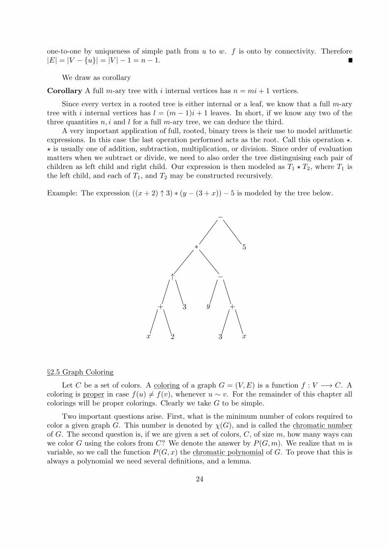
A very important application of full, rooted, binary trees is their use to model arithmeticexpressions. In this case the last operation performed acts as the root. Call this operation ⋆.⋆ is usually one of addition, subtraction, multiplication, or division. Since order of evaluationmatters when we subtract or divide, we need to also order the tree distinguising each pair ofchildren as left child and right child. Our expression is then modeled as T1 ⋆ T2, where T1 isthe left child, and each of T1, and T2 may be constructed recursively.

Example: The expression ((x+ 2) ↑ 3) ∗ (y − (3 + x))− 5 is modeled by the tree below.

−

∗ 5

↑ −

+ 3 y +

x 2 3 x

.....................................................................................................

.....................................................................................................

........................................................................................................

........................................................................................................

....................................................................................

....................................................................................

....................................................................................

....................................................................................

....................................................................................

....................................................................................

....................................................................................

....................................................................................

§2.5 Graph Coloring

Let C be a set of colors. A coloring of a graph G = (V,E) is a function f : V −→ C. Acoloring is proper in case f(u) = f(v), whenever u ∼ v. For the remainder of this chapter allcolorings will be proper colorings. Clearly we take G to be simple.

Two important questions arise. First, what is the minimum number of colors required tocolor a given graph G. This number is denoted by χ(G), and is called the chromatic numberof G. The second question is, if we are given a set of colors, C, of size m, how many ways canwe color G using the colors from C? We denote the answer by P (G,m). We realize that m isvariable, so we call the function P (G, x) the chromatic polynomial of G. To prove that this isalways a polynomial we need several definitions, and a lemma.

24

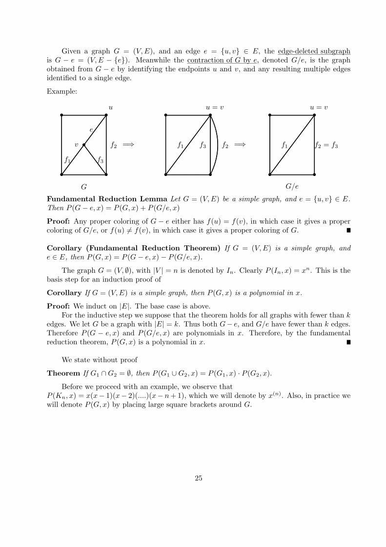
Given a graph G = (V,E), and an edge e = {u, v} ∈ E, the edge-deleted subgraphis G − e = (V,E − {e}). Meanwhile the contraction of G by e, denoted G/e, is the graphobtained from G − e by identifying the endpoints u and v, and any resulting multiple edgesidentified to a single edge.

Example:

G

e

u

v

f1

f2

f3

u = v

f1 f2f3

u = v

f1 f2 = f3

G/e

=⇒ =⇒

• •

•

• •

• •

• •

•

•

•

•

................................................................................................................................................................................................................................................................................................................................................................

..............................................................................................................................

..............................................................................................................................

.....................................................................................................................................................................................................................................................................................

.........................................................................................................................................................................................................

.......................................................................................................................................................

...........................................................................................................................................................................................................................................................

.........................................................................................................................................................................................................................................................................................................................................................................................................................................................................................................................................................................

.........................................................................................................................................................................................................

.......................................................................................................................................................

...........................................................................................................................................................................................................................................................

................................................................................................................................................................................................................................................................................................................................................................

.................................................................................................................................................................................................................

Fundamental Reduction Lemma Let G = (V,E) be a simple graph, and e = {u, v} ∈ E.Then P (G− e, x) = P (G, x) + P (G/e, x)

Proof: Any proper coloring of G − e either has f(u) = f(v), in which case it gives a propercoloring of G/e, or f(u) = f(v), in which case it gives a proper coloring of G.

Corollary (Fundamental Reduction Theorem) If G = (V,E) is a simple graph, ande ∈ E, then P (G, x) = P (G− e, x)− P (G/e, x).

The graph G = (V, ∅), with |V | = n is denoted by In. Clearly P (In, x) = xn. This is thebasis step for an induction proof of

Corollary If G = (V,E) is a simple graph, then P (G, x) is a polynomial in x.

Proof: We induct on |E|. The base case is above.For the inductive step we suppose that the theorem holds for all graphs with fewer than k

edges. We let G be a graph with |E| = k. Thus both G− e, and G/e have fewer than k edges.Therefore P (G − e, x) and P (G/e, x) are polynomials in x. Therefore, by the fundamentalreduction theorem, P (G, x) is a polynomial in x.

We state without proof

Theorem If G1 ∩G2 = ∅, then P (G1 ∪G2, x) = P (G1, x) · P (G2, x).

Before we proceed with an example, we observe thatP (Kn, x) = x(x− 1)(x− 2)(....)(x− n+1), which we will denote by x(n). Also, in practice wewill denote P (G, x) by placing large square brackets around G.

25

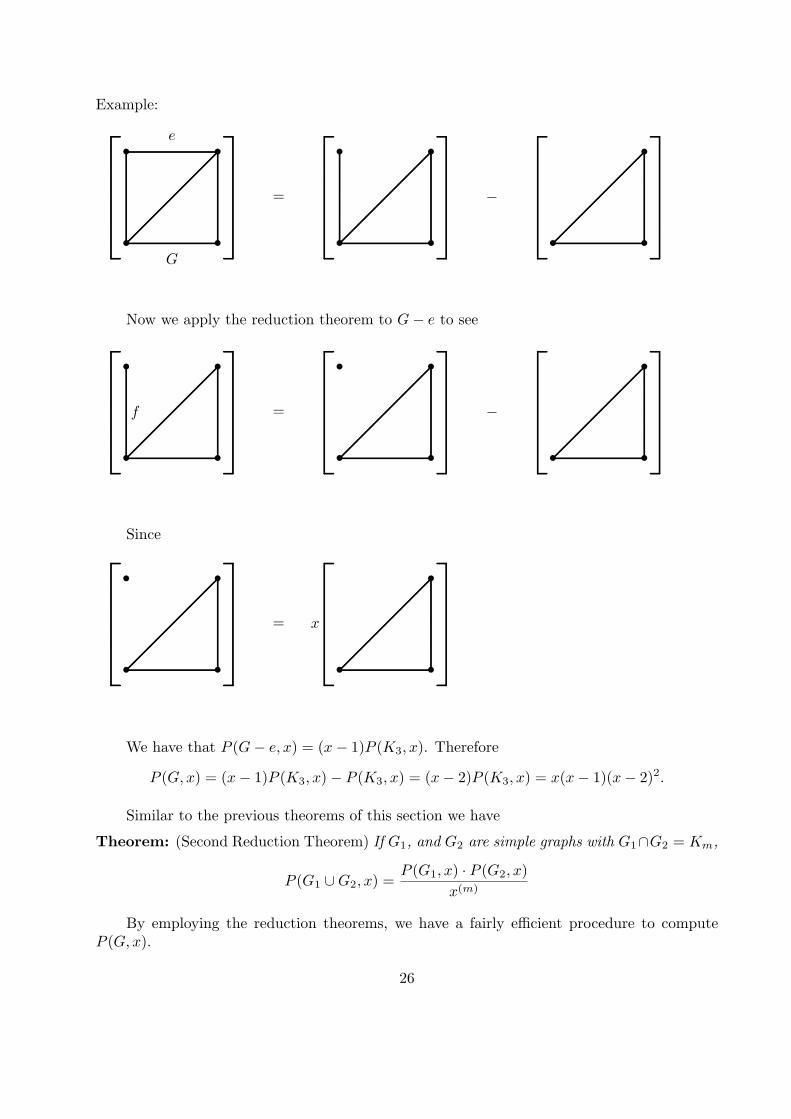
Example:

e

G

= −

• •

• •

• •

• •

•

• •

.................................................................................................................................................................................................................................................................................................................................................................................................................................................................................................................................................................................................................................................................................................................................................................................................................................................

.............

.............

.............

.............

.............

.............

.............

.............

.............

.............

.............

.............

.............

.............

.............

......

................

................ .........................................................................................................................................................................................................

................

................

...................................................................................................................................................................................................................................................................................................................................................................................................................................................................................................................................

.............

.............

.............

.............

.............

.............

.............

.............

.............

.............

.............

.................................................................................................................................................................................................................

................

................

.........................................................................................................................................................................................................

................

................

.....................................................................................................................................................................................................................

..............................................................................................................................................................................................................................................................................................................

.........................................................................................................................................................................................................

................

................

.........................................................................................................................................................................................................

................

................

Now we apply the reduction theorem to G− e to see

f = −

• •

• •

• •

• •

•

• •

..........................................................................................................................................................................................................................................................................................................................................................................................................................................................................................................................................................................................................................................................................................

.............

.............

.............

.............

.............

.............

.............

.............

.............

.............

.............

.............

.............

.............

.............

......

................

................ .........................................................................................................................................................................................................

................

............................................................................................................................................................................................................................................................................................................................................................................................

.............

.............

.............

.............

.............

.............

.............

.............

.............

.............

.............

.................................................................................................................................................................................................................

................

................

.........................................................................................................................................................................................................

................

................

.....................................................................................................................................................................................................................

..............................................................................................................................................................................................................................................................................................................

.........................................................................................................................................................................................................

................

................

.........................................................................................................................................................................................................

................

................

Since

= x

• •

• •

•

• •...................................................................................................................................................................................................................................................................................................................................................................................................................................................................................................................................

.............

.............

.............

.............

.............

.............

.............

.............

.............

.............

.............

.............

.............

.............

.............

......

................

................ .........................................................................................................................................................................................................

................

............................................................................................................................................................................................................................................................................................................................................................................................

.............

.............

.............

.............

.............

.............

.............

.............

.............

.............

.............

.................................................................................................................................................................................................................

................

................

.........................................................................................................................................................................................................

................

................

We have that P (G− e, x) = (x− 1)P (K3, x). Therefore

P (G, x) = (x− 1)P (K3, x)− P (K3, x) = (x− 2)P (K3, x) = x(x− 1)(x− 2)2.

Similar to the previous theorems of this section we have

Theorem: (Second Reduction Theorem) If G1, and G2 are simple graphs with G1∩G2 = Km,

P (G1 ∪G2, x) =P (G1, x) · P (G2, x)

x(m)

By employing the reduction theorems, we have a fairly efficient procedure to computeP (G, x).

26

This in turn allows us to compute χ(G). We observe that the value of P (G, x) willbe zero whenever x is a non-negative whole number strictly smaller than χ(G). So χ(G) ischaracterized as being the smallest non-negative integer for which P (G, x) = 0.

In addition, by the factor theorem from basic algebra, if χ(G) = k we can always writeP (G, x) in the form xe1(x − 1)e2(x − 2)e3 ...(x − (k − 1))ekg(x), where the exponents ei arepositive and g(x) is a polynomial with no integral roots. Conversely, writing P (G, x) in thisform allows us to deduce χ(G) = k.

Warning: A common mistake occurs when someone finds a coloring of G using k colors anddeduces that χ(G) = k. The correct deduction is χ(G) ≤ k. To show equality we must eitheruse the idea above, or perhaps the last theorem.

Theorem: If G is a simple graph with an induced subgraph isomorphic to Km, then χ(G) ≥ m.

27

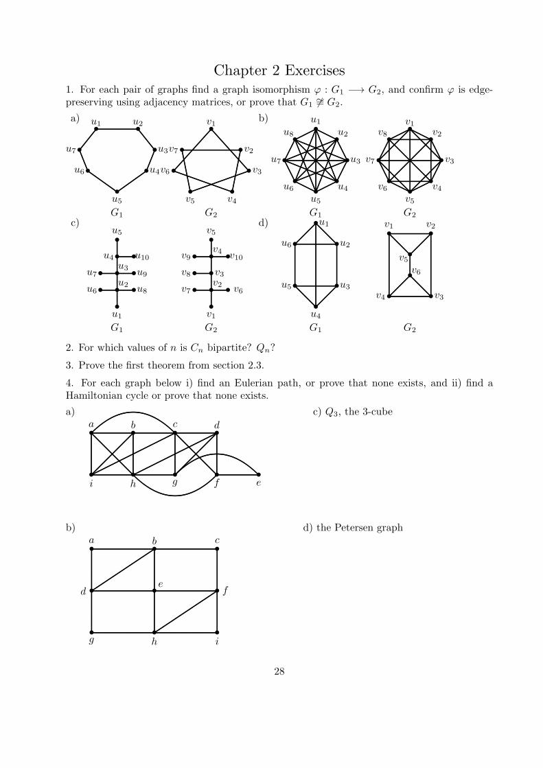
Chapter 2 Exercises1. For each pair of graphs find a graph isomorphism φ : G1 −→ G2, and confirm φ is edge-preserving using adjacency matrices, or prove that G1 ∼= G2.

a) b)

c) d)G1 G2 G1 G2

G1 G2 G1 G2

u1 u2

u3

u4

u5

u6

u7

v1

v2

v3

v4v5

v6

v7

u1

u2

u3

u4

u5

u6

u7

u8

v1v2

v3

v4v5

v6

v7

v8

u1

u2

u3

u4

u5

u6

u7

u10

u8

u9

v1

v2v3

v4

v5

v6v7

v8

v9 v10

u1

u2

u3

u4

u5

u6

v1 v2

v3v4

v5v6

• •

• •

• •

•

•

• •

• •

• •

••

••

•

•

•

•••

••

•

•

•

•

•••••

• •• •

•

•••••

• ••• •

•

• •

• •

•

• •

• •

•

•

...............................................................................................................................................................................................................................................................................................................................................................

............................................

...................................................................................................................... .........................................................................................................................................................................................................................................................................................................

..................................................................................................................................................................................................................................................................................................................................................................................

............................................................................

.......................................................................................................................................................................... ........................................................

.......................................................................................................................................

.......................................................................................................................................................

.......................................................................................................................................

........................................................ ........................................................

.......................................................................................................................................

..............................................................................................................................................

....................................................................................................................................... ........................................................

.......................................................................................................................................

....................................................................................................................................................... ....................................................................

...................................................................

........................................................

....................................................................

...................................................................

....................................

....................................

....................................

..................................

........................................................

.......................................................................................................................................

................................................................................................................

........................................................

...........................................................................................................

.......................................................................................................................................................

...........................................................................................................

........................................................ ........................................................

.....................................................................................................

..............................................................................................................................................

.....................................................................................................

........................................................

...........................................................................................................

.......................................................................................................................................................

........................................................

..................................................................................................... ....................................

....................................

....................................

..................................

........................................................

....................................

....................................

...................................

........................................................

.............

.............

.............

.............

.............

.............

.............

..........

........................................................

.............

.............

.............

........................................... .................................................

.............

.............

........................................... ......................................................

.............

.............

........................................................

.............

.............

..

.............

.............

.............

.................................................................................... .............

.............

.............

........................................... .............

.............

.............

........................................... ......................................................

.............

.............

..

.......................................................................

.........................................................................................................................................................................................................

....................................................................... ..................................................................................................... ............................................................................................................................................................................

.....................................................................................................

....................................

........................................................................................................................................

............................................................................................................................................................................

.......................................................................................................................................................

.......................................................................

.......................................................................................................................................................

..........................................................................................................................

....................................................................... .....................................................................................................

2. For which values of n is Cn bipartite? Qn?

3. Prove the first theorem from section 2.3.

4. For each graph below i) find an Eulerian path, or prove that none exists, and ii) find aHamiltonian cycle or prove that none exists.

a) c) Q3, the 3-cubea b c d

efghi

• • • •

•••••

...........................................................................................................................................................................................................................................................................................................................................................................................................................................................................................................................................................................................................................

..............................................................................................................................................

..............................................................................................................................................

.............................................................................................................................................................

........................................................

........................................................

.............................................................................................................................................................

..............................................................................................................................................

................................................................................................................................................................................................................................

..............................................................................................................................................

..........................................................................................................................................................................................................

......................................................................................................................................................................................................................................

............................................................................................................................................................................................................................................................................................................................................................................................................................................................................

b) d) the Petersen grapha b c

de

f

g h i

• • •

• • •

• • •

...................................................................................................................................................................................................................................................................................................................................................................................................................................................................................................................................................................................................................................................................................................................................................................................................................................

.............................................................................................................................................................................................................................................................................................................

.........................................................................................................................................................................................................

.........................................................................................................................................................................................................

.....................................................................................................................................................................................

.....................................................................................................................................................................................

28

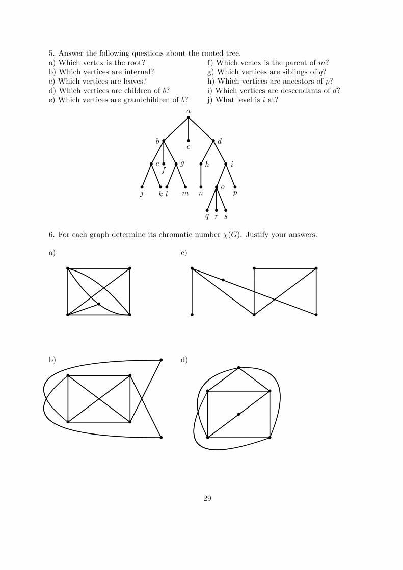
5. Answer the following questions about the rooted tree.a) Which vertex is the root? f) Which vertex is the parent of m?b) Which vertices are internal? g) Which vertices are siblings of q?c) Which vertices are leaves? h) Which vertices are ancestors of p?d) Which vertices are children of b? i) Which vertices are descendants of d?e) Which vertices are grandchildren of b? j) What level is i at?

a

bc

d

ef

g h i

j k l m no

p

q r s

•

• • •

• • • • •

• • • • • • •

• • •

..............................................................................................................

............................................................................

....................................................................................................................................................................................................

............................................................................

......................................................................................

......................................................................................

.......................................................................................................................................................................

.................................................................................

.................................................................................

.................................................................................

............................................................................

.................................................................................

..................................................................................................................................................................

............................................................................

.................................................................................

6. For each graph determine its chromatic number χ(G). Justify your answers.

a) c)

• •

•• •

• • •

• • •

•....................................................................................................................................................................................................................................................................................................................................................................................................................................................................................................................................................................................................................................................................................................................................................................................................................................

............................................................................

..............................

.......................................................................................................................................................

.......................................................................................................................................................

...........................................................................................................................................................................................................................................................

............................................................................................................................................................................................................................................................................................................................................................................................................................................

.......................................................................................................................................................

.........................................................................................................................................................................................................

..................................................................................................................................................................................................................................................................................................................................................................................................................

......................................................................................................................................................................................................................................................................

...............................................................................................................................................................................................................................................................

b) d)

• •

•

•

• •

• •

•

•

• •

................................................................................................................................................................................................................................................................................................................................................................

...........................................................................................................................................................................................................................................................

...........................................................................................................................................................................................................................................................

.......................................................................................................................................................

................................................................................................................................................................................................................................

................................................................................................................................................................................................................................

.........................................................................................................................................................................................................

................................................................................................................................................................................................................................................................................................................................................................

..............................................................................................................................

...........................................................................................................................................................................................................................................................

.........................................................................................................................................................................................................

..........................................

..........................................

..........................................

.......................................................................................................................................................

......................

......................................................................................................................................................................................................................

..............................................................................................................................

.........................................................................................................................................................................................

...................................................................................................................................................................................................................................................................................................................................................................................................................................................................................................................................................................

.....................................................................................................................................................................................................................................................................................................................

.....................................................................................................................................................................................................................................................................................................................................

.........................................................................................................................................................................................................................................................................................................................................................................................................

................................

29

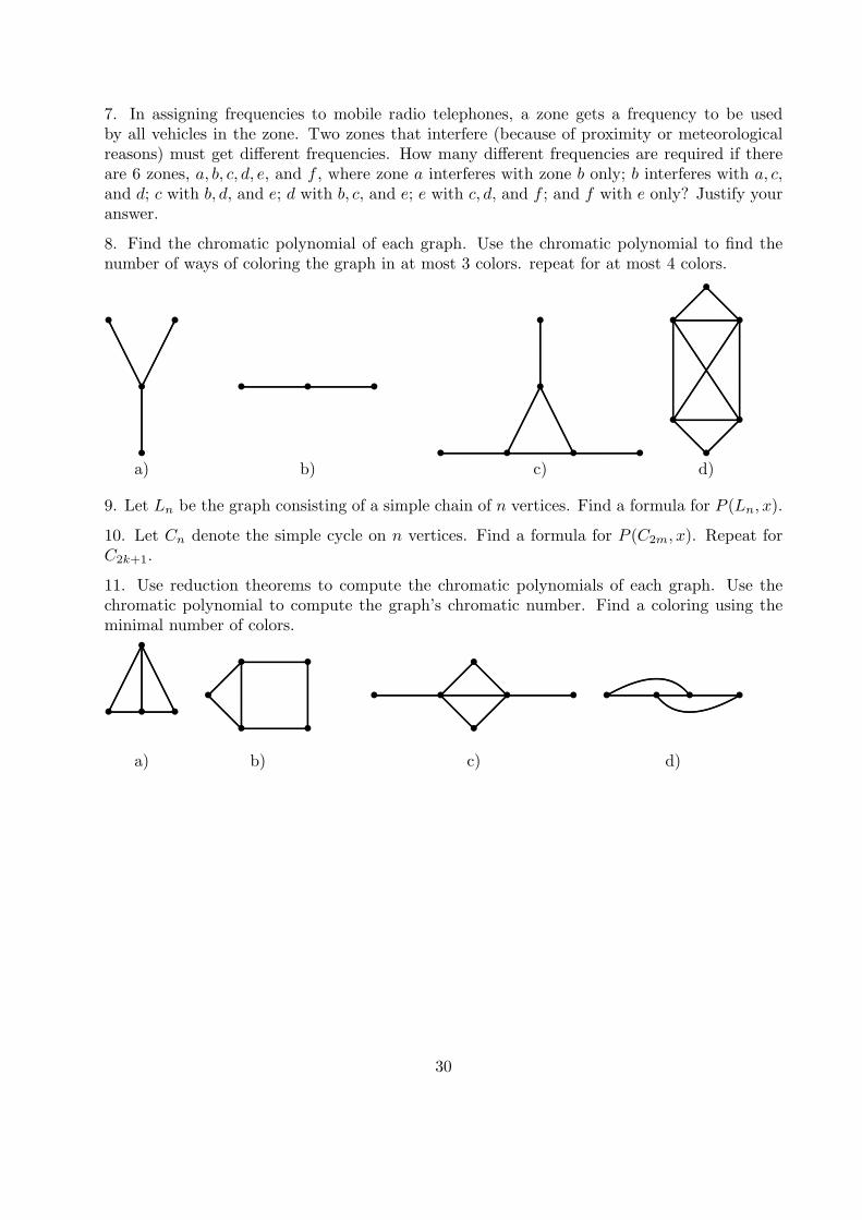
7. In assigning frequencies to mobile radio telephones, a zone gets a frequency to be usedby all vehicles in the zone. Two zones that interfere (because of proximity or meteorologicalreasons) must get different frequencies. How many different frequencies are required if thereare 6 zones, a, b, c, d, e, and f , where zone a interferes with zone b only; b interferes with a, c,and d; c with b, d, and e; d with b, c, and e; e with c, d, and f ; and f with e only? Justify youranswer.

8. Find the chromatic polynomial of each graph. Use the chromatic polynomial to find thenumber of ways of coloring the graph in at most 3 colors. repeat for at most 4 colors.

a) b) c) d)

• •

•

•

• • •

• • • •

•

•

•

• •

••

•.............................................................................................................................................................................................................................................................................................................................................................................................................................

.....................................................................................................................................................................................................................

.........................................................................................................................................................................................................

................................................................................................................................................................................................................................

.....................................................................................................

.......................................................................

.......................................................................

.......................................................................

....................................

...................................

.......................................................................................................................................................

...............................................................................................................................................................................................................................................................................................................................................................................................................................................................................

.....................................................................................................

.......................................................................................................................................................

9. Let Ln be the graph consisting of a simple chain of n vertices. Find a formula for P (Ln, x).

10. Let Cn denote the simple cycle on n vertices. Find a formula for P (C2m, x). Repeat forC2k+1.

11. Use reduction theorems to compute the chromatic polynomials of each graph. Use thechromatic polynomial to compute the graph’s chromatic number. Find a coloring using theminimal number of colors.

a) b) c) d)

•

• • ••

•

•

•

•

• • • •

•

•

• • • •................................................................................................................

..........................................................................................................................................................................................................

................................................................................................................

.......................................................................

.......................................................................

.....................................................................................................

...............................................................................................................................................................................................................................................................................................................

.................................................................................................................................................................................................................................................................................................................................................

...................................

.......................................................................

.......................................................................

.......................................................................

...................................................................................................................................................................................................................................................................................................................................................................................................................................................................

............................

30

Chapter 3: Intermediate CountingWe saw at the end of chapter 1 that there are problems which can easily be posed, which

do not admit solutions by the tactics of basic counting. In this chapter we develop furthertactics, in part to rectify this apparent short-fall of basic counting.

§3.1 Generating Functions

If f is a smooth enough function near x = 0 it can be expanded (maybe via Taylor’sTheorem) in terms of a Maclaurin Series. That is, in some neighborhood of x = 0, there

is no difference between the function f(x), and the values of the power series

∞∑k=0

akxk. In

fact Taylor’s Theorem tells us that the coefficients ak = f (k)(0)/k!, where f (k)(x) is the kthderivative of f(x).

If f(x) =

∞∑k=0

akxk, for all values of x in some neighborhood of x = 0, we say that f(x) is

the (ordinary) generating function for the sequence of coefficients

(ak

)∞

k=0

.

Example: f(x) =1

1− x= 1 + x+ x2 + x3 + ... =

∞∑k=0

xk, for |x| < 1, so f(x) generates the

constant sequence

(1, 1, 1, 1, 1, .....

)=

(1

)∞

k=0

.

Example: f(x) = (1 + x)4 = 1 + 4x + 6x2 + 4x3 + x4, for all x ∈ IR, so f(x) generates the

sequence

(1, 4, 6, 4, 1, 0, 0, 0....

)=

((4

k

))∞

k=0

.

Our first challenge is to develop a set of tools which allow us to build a library of basicgenerating functions.

Theorem: If f(x) generates the sequence

(an

)∞

n=0

, and g(x) generates the sequence

(bn

)∞

n=0then

1) f(x)± g(x) generates the sequence

(an ± bn

)∞

n=0

.

2) f(x)g(x) generates the sequence

(cn

)∞

n=0

, where ck =k∑

l=0

albk−l.

3) f ′(x) generates the sequence

(a1, 2a2, 3a3, ...

)=

((n+ 1)a+ n+ 1

)∞

n=0

.

4) The function F (x), with F (0) = 0 and F ′(x) = f(x), generates

(0, a0,

a12,a23, ...

).

Proof: See your favorite calculus II textbook.

Notice that we can also deduce that xf ′(x) generates

(nan

)∞

n=0

. Also if F is as in part

4, then F (x)/x generates

(an

n+ 1

)∞

n=0

.

31

Finally we remark that we may replace the symbol x with all sorts of things formally, anddeduce new and fun-filled facts.

Example: Since1

1− x, generates

(1n

)∞

n=0

,1

1− 2xgenerates

(2n

)∞

n=0

.

Also1

1 + xgenerates

((−1)n

)∞

n=0

.

Example: From the previous example,

∫dx

1 + x=

∫ [ ∞∑n=0

(−1)nxn

]dx

Now technically we can only interchange the order of integration and summation if we havethe right kind of convergence of our power series. Since we are only interested in formalmanipulation of power series, we’ll not worry about this subtlely here, nor henceforth. Thus

ln(1 + x) =

∫dx

1 + x=

∞∑n=0

[(−1)n

∫xn dx

]=

[ ∞∑n=0

(−1)nxn+1

n+ 1

]+ C

The value of C is found to be 0 by substituting in x = 0 and evaluating ln(1) = 0. So

ln(1 + x) generates the sequence

((−1)n

n+ 1

)∞

n=0

.

Example: Similar to the previous example we can start with1

1− x=

∞∑n=0

xn. We differentiate

both sides of the equation with respect to x, interchanging the order of differentiation and

summation on the right-hand side. We arrive at1

(1− x)2=

∞∑n=1

nxn−1 =

∞∑m=0

(m+ 1)xm. Thus

x

(1− x)2=

∞∑m=0

(m+ 1)xm+1 =∞∑k=0

kxk generates the sequence

(k

)∞

k=0

.

§3.2 Applications to Counting

Consider the generating function (1 + x)4 = 1 + 4x + 6x2 + 4x3 + x4 + 0x5 + 0x6 + ...,

which generates the sequence

((4

k

))∞

k=0

, whose terms are the number of k-subsets of a 4-set.

This function is the result of evaluating the expression (1 + ax)(1 + bx)(1 + cx)(1 + dx) ata = b = c = d = 1. The expansion of this function gives

1 + (a+ b+ c+ d)x+ (ab+ ac+ ad+ bc+ bd+ cd)x2 + (abc+ abd+ acd+ bcd)x3 + (abcd)x4.

The coefficients of xi in this expansion clearly describe all of the subsets of {a, b, c, d} of size i.More generally it occurs to us that the coefficient of xk in the expansion of (1+x)n is the

number of k-subsets of an n-set. If we write the expansion of (1+a1x)(1+a2x)(1+a3x)...(1+anx), then the coefficient of xk is an ordered list describing all k-subsets of {a1, a2, ..., an}. Infact (1 + x)n results if we set ai = 1, for i = 1 to n, in the expression (1 + a1x)(1 + a2x)(1 +a3x)...(1 + anx).

Now what about (1 + ax + a2x2 + a3x3)(1 + bx + b2x2)(1 + cx)? Upon expansion wefind this is 1 + (a + b + c)x + (a2 + ab + ac + b2 + bc)x2 + (a3 + a2b + a2c + ab2 + abc +

32

b2c)x3 + (a3b + ac + a2b2)x4 + (a3b2 + a3bc)x5 + (a3b2c)x6. Setting a = b = c = 1 we have(1 + x + x2 + x3)(1 + x + x2)(1 + x) = 1 + 3x + 5x2 + 6x3 + 3x4 + 2x5 + x6. So what is thecombinatorial significance of this sequence?

After a little thought, and considering the coefficients in the first expansion, we realize thiscounts the number of solutions in non-negative integers to y1+y2+y3 = i, where y1 ≤ 3, y2 ≤ 2,and y3 ≤ 1. Which is to say that the first expression generates all multisets of size i from{a, b, c}, using at most 3 a’s, at most 2 b’s, and at most one c.

In general we wish to compute the number of integral solutions to y1 + y2 + ...+ yk = r,where ai ≤ yi ≤ bi, i = 1, ...k, and the ai’s and bi’s are integral lower and upper bounds. Todo this we can now use a generating function approach. We simply compute the coefficient

of xr in the expansion ofk∏

i=1

(xai + xai+1 + xai+2 + ...+ xbi) =k∏

i=1

[

bi∑j=ai

xj ]. Probably we get a

computer algebra system to do this for us. Again we would use a computer algebra system if we

used place-holders di, i = 1, ..., k to generate the actual solutions, i.e. expandedk∏

i=1

[

bi∑j=ai

(dix)j ].

Naturally we could re-index the problem to count the number of solutions in non-negativeintegers to y1 + ... + yk = s, where yi ≤ ci = bi − ai, and s = r − a1 − a2 − ... − ak. Now we

need the coefficient of xs in the expansion ofk∏

i=1

(1 + x+ x2 + ...+ xci) =k∏

i=1

[

ci∑j=0

xj ].

And, as might happen in an ideal world, we might have s ≤ ci for all i, so that there areeffectively no upper bounds. Here we want to realize that the coefficient of xs in the expansion

ofk∏

i=1

(1 + x+ x2 + ...+ xci) =k∏

i=1

[

ci∑j=0

xj ], is the same as the coefficient of xs in the expansion

ofk∏

i=1

(1 + x+ x2 + ...) =k∏

i=1

[∞∑j=0

xj ] =k∏

i=1

1

1− x= (1− x)−k. So apparently

(1− x)−k generates the sequence

((s+ k − 1

s

))∞

s=0

??!!

Amazingly this little gem of information can also be derived from the general version ofthe Binomial Theorem discovered by Isaac Newton.

Theorem(Newton) For any real number u = 0, (1 + x)u =

∞∑k=0

(u

k

)xk, where(

u

k

)= u(u− 1)(u− 2)...(u− k + 1)/k!.

When we set u = −p, where p is a positive integer we find that(−pk

)=

(−p)(−p− 1)(−p− 2)...(−p− k + 1)

k!

= (−1)k (p+ k − 1)(p+ k − 2)...(p+ 1)p

k!

= (−1)k(p+ k − 1

k

)33

So replacing x by −x in the theorem we arrive at

(1− x)−p =

∞∑k=0

(−pk

)(−x)k

=∞∑k=0

(−1)k(p+ k − 1

k

)(−1)kxk

=∞∑k=0

(p+ k − 1

k

)xk

since (−1)k(−1)k = (−1)2k = 1. Thus (1 − x)−p generates the number of solutions to thedonut shoppe problem.

Before we leave this topic we remark that there are other directions in which we mightgeneralize. For example, the number of ways to make n cents change using pennies, nickels,dimes and quarters is the number of solutions in non-negative integers to

y1 + 5y2 + 10y3 + 25y4 = n.

This is also the coefficient of xn in the expansion of (1−x)−1(1−x5)−1(1−x10)−1(1−x25)−1.So we can use generating functions to compute the number of, and enumerate the solutions toa great variety of linear diophantine equations.

§3.3 Exponential Generating Functions

As we saw in chapter 1, Stirling Numbers of the second kind are important for countingsolutions to occupancy problems. In order to derive the formula given for S(n, k) in chapter1, we will use exponential generating functions.

If f(x) =

∞∑k=0

akk!

xk, for all values of x in some neighborhood of x = 0, we say that f(x) is

the exponential generating function for the sequence of coefficients

(ak

)∞

k=0

.

So, for example, f(x) = ex is the exponential generating function for

(1

)∞

k=0

. And in

general g(x) = eαx is the exponential generating function for

(αk

)∞

k=0

.

Next we recall that combinations and permutations are related by P (n, k) = k!C(n, k),or P (n, k)/k! = C(n, k). Similar formulas apply when some repetition is allowed, ala theMISSISSIPPI problem. So we consider the expansion of

(1 +a

1!x+

a2

2!x2 +

a3

3!)((1 +

b

1!x+

b2

2!x2)((1 +

c

1!x)

which comes out to

34

1 + (a

1!+

b

1!+

c

1!)x+ (

a2

2!+

ab

1!1!+

ac

1!1!+

b2

2!+

bc

1!1!)x2+

(a3

3!+

a2b

2!1!+

a2c

2!1!+

ab2

1!2!+

abc

1!1!1!+

b2c

2!1!)x3 + (

a3b

3!1!+

a3c

3!1!+

a2b2

2!2!+

a2bc

2!1!1!+

ab2c

1!2!1!)x4 + (

a3b2

3!2!+

a3bc

3!1!1!+

a2b2c

2!2!1!)x5 + (

a3b2c

3!2!1!)x6

Next we multiply and divide the coefficient of xk by k! to get

1 + 1!(a

1!+

b

1!+

c

1!)x

1!+ 2!(

a2

2!+

ab

1!1!+

ac

1!1!+

b2

2!+

bc

1!1!)x2

2!+

3!(a3

3!+

a2b

2!1!+

a2c

2!1!+

ab2

1!2!+

abc

1!1!1!+

b2c

2!1!)x3

3!+ 4!(

a3b

3!1!+

a3c

3!1!+

a2b2

2!2!+

a2bc

2!1!1!+

ab2c

1!2!1!)x4

4!+ 5!(

a3b2

3!2!+

a3bc

3!1!1!+

a2b2c

2!2!1!)x5

5!+ 6!(

a3b2c

3!2!1!)x6

6!

Now, for example, the coefficient on a “sub-multi-set” term like a2b2c, is the number of 5-strings over {a, b, c} using 2 a’s, 2 b’s and 1 c. So setting a = b = c = 1, we can generate thenumber of permutations with partial replacement over a given alphabet.

Theorem: Given r types of objects, with ei indistinguishable objects of type i, i = 1, 2, ..., r,the number of distinguishable permutations of length k using up to ei objects of type i is thecoefficient of xk/k! in the exponential generating function(

1 +x

1!+

x2

2!+ ...+

xe1

e1!

)(1 +

x

1!+ ...+

xe2

e2!

)....

(1 +

x

1!+ ...+

xer

er!

)As a final application of exponential generating functions we derive the formula

S(n, k) =1

k!

k∑i=0

(−1)i(k

i

)(k − i)n.

We find T (n, k) = k!S(n, k) = # onto functions from an n-set to a k-set = the number ofn-permutations of a k-set using each set element at least once. So T (n, k) is the coefficient ofxk/k! in the expansion of (

x+x2

2!+

x3

3!+ ....

)k

= (ex − 1)k.

By the binomial theorem

(ex − 1)k =k∑

i=0

(k

i

)(−1)ie(k−i)x

=k∑

i=0

(k

i

)(−1)i

∞∑n=0

(k − i)nxn

n!

=∞∑

n=0

xn

n!

k∑i=0

(k

i

)(−1)i(k − i)n

35

where the second equation is from the Maclaurin series for ex, and the order of summationcan be reversed since the Maclaurin series for ex converges absolutely on the entire real line.

So we have T (n, k) =k∑

i=0

(k

i

)(−1)i(k − i)n, and thus S(n, k) is as stated.

§3.4 Recurrence Relations

Given a sequence, a, with domain D = {n ∈ ZZ|n ≥ m} and codomain IR, a recurrencerelation is a formula which for all n ∈ {l ∈ ZZ|l ≥ k} (where k ≥ m) relates an, in somemanner, to a finite number of preceding terms of the sequence and possibly a function of n.

We will almost exclusively be interested in recurrence relations which take the form

an = c1an−1 + c2an−2 + ...+ ckan−k + f(n)

where c1, c2, ..., ck ∈ IR, and ck = 0. Such a recurrence relation is a linear recurrence relationwith constant coefficients. When the function f(n) = 0, we call the recurrence relationhomogeneous. If f(n) is not identically zero, the recurrence relation is non-homogeneous.The number k is called the degree of the relation.WARNING: A formula which recursively defines a sequence does not completely determinethe sequence. Observe, for example, that geometric sequences with common ratio r all satisfyan = r · an−1, for n ≥ 1. What picks out a single sequence in this case is its initial term. Ingeneral we may need to know several initial terms, which are called the initial conditions ofthe sequence. Given a sufficient number of initial conditions, and a recurrence relation, we getexactly one sequence of real numbers.

Example: Suppose that we deposit A0 dollars in an account drawing t percent interest perannum compounded yearly, and that no withdrawals occur. Then if An denotes the money inthe account after n years, we have An = (1 + t

100 )An−1, when n ≥ 1.

In this simplest of all cases, it is clear that the initial condition is of paramount importance.It’s also true that we can find an explicit formula for An in this case since the sequence isgeometric. In short An = rn · A0, where r = (1 + t

100 ). We call this process solving therecurrence relation. In this example we solved it by inspection. The general case is moredifficult and is the topic of the next section.

Example: A canonical example relates the story of the Towers of Hanoi. A group of monkswished a magical tower to be constructed from 1000 stone rings. The rings were to be of 1000different sizes. The size and composition of the rings was to be designed so that any ring couldsupport the entire weight of all of the rings smaller than itself, but each ring would be crushedbeneath the weight of any larger ring.

The monks hired the lowest bidder to construct the tower in a clearing in the dense junglenearby. Upon completion of construction the engineers brought the monks to see their work.The monks admired the exquisite workmanship, but informed the engineers that the towerwas not in the proper clearing.

In the jungle there were only three permanent clearings. The monks had labelled themA, B and C. The engineers had labelled them in reverse order. The monks instructed theengineers to move the tower from clearing A to clearing C!

36

Because of the massive size of the rings, the engineers could only move one per day. Noring could be left anywhere in the jungle except one of A, B, or C. Finally each clearing wasonly large enough so that rings could be stored there by stacking them one on top of another.

The monks then asked the engineers how long it would take for them to fix the problem.Before they all flipped a gasket, the most mathematically talented engineer came upon

the following solution.Let Hn denote the minimum number of days required to move an n ring tower from A to

C under the constraints given. Then H1 = 1, and in general an n ring tower can be movedfrom A to C by first moving the top (n − 1) rings from A to B leaving the bottom ring atA, then moving the bottom ring from A to C, and then moving the top (n − 1) rings fromclearing B to clearing C. So Hn = 2 ·Hn−1 + 1, for n ≥ 2.

By unwinding this sequence similar to the one at the end of section 2.4 we get

Hn = 2 ·Hn−1 + 1

= 2 · [2 ·Hn−2 + 1] + 1 = 22 ·Hn−2 + 2 + 1

= 22 · [2 ·Hn−3 + 1] + 2 + 1 = 23 ·Hn−3 + 22 + 2 + 1

...

At the kth iteration

Hn = 2kHn−k + 2k−1 + 2k−2 + ...+ 23 + 22 + 2 + 1

...

= 2n−1Hn−(n−1) + 2n−2 + ...+ 22 + 2 + 1

= 2n−1H1 + 2n−2 + ...+ 22 + 2 + 1

=n−1∑l=0

2l, since H1 = 1

= 2n − 1, by the geometric sum formula

So the problem would be fixed in 21000 − 1 days, or approximately 2.93564× 10296 centuries.Hence the term job security!

Example: A more realistic example might be to count the number of binary strings of lengthn ≥ 0 which contain a pair of consecutive 0’s.

Here we let bn denote the binary strings which have length n and contain a pair ofconsecutive zeroes. We can find b0 = b1 = 0 by inspection, as well as b2 = 1.

To find b3 we write down all bit strings of length 3 and cross out those which do not havea pair of consecutive zeroes. What’s left is 000, 001 and 100. So b3 = 3.

Similarly b4 = 8 since the strings of length 4 which contain a pair of consecutive zeroesare 0000, 0001, 0010, 0011, 0100, 1000, 1001, and 1100. We might continue this time-consumingand tedious process hoping to discover a pattern by sheer luck, or we can attempt to use acombinatorial approach.

Let Sk denote the bit strings of length k which contain a pair of consecutive zeroes. Noticethat |Sk| = bk.

37

If x ∈ Sn, then either x = 1y, where y ∈ Sn−1, or x = 0w, where w is a bit string oflength n − 1. In case x = 0w, either x = 01z, where z ∈ Sn−2, or w = 00v, where v is anybinary string of length n− 2. Since these sub-cases are exclusive, by the addition principle

bn = bn−1 + bn−2 + 2n−2, for n ≥ 2.

Together with the initial conditions b0 = b1 = 0, this completely determines the sequence. Agood check is that the terms we generated actually satisfy this relation. Of course we probablywould not want to use the recursive definition to find b128. This motivates the next section.

§3.5 The Method of Characteristic Roots

In the last section we noted that any homogeneous linear recurrence relation of degree 1with constant coefficient corresponds to a geometric sequence. These can therefore be solvedby inspection. Also from the Towers of Hanoi story one might guess correctly that most non-homogeneous linear recurrence relations with constant coefficients can be solved by unwinding.Neither of these methods is powerful enough in general. So in this section we introduce a basicmethod for solving homogeneous linear recurrence relations with constant coefficients.

We begin by considering the case k = 2. So we have a recurrence relation of the forman = c1an−1 + c2an−2, for n ≥ m, where c1 and c2 are real constants. We must also havetwo initial conditions am−1 and am−2 to get started at n = m. We will dispense with thegeneral case here and suppose that m = 2. That is, we are given a0 and a1 and the formulaan = c1an−1 + c2an−2, for n ≥ 2. Notice that c2 = 0 or else we have a linear recurrencerelation with constant coefficients and degree 1. What we seek is a closed form expression foran, which is a function of n alone, and which is therefore independent of the previous termsof the sequence.

Of fundamental importance to this method is the characteristic polynomial, denoted χ(x)of the recurrence relation. For the case above we define χ(x) = x2 − c1x − c2. Notice thatthe degree of χ(x) coincides with the degree of the recurrence relation. Notice also that thenon-leading coefficients of χ(x) are simply the negatives of the coefficients of the recurrencerelation. This allows us to generalize the definition so that the characteristic polynomial ofan = c1an−1 + ... + ckan−k is χ(x) = xk − c1x

k−1 − ... − ck−1x − ck. A number r (possiblycomplex) is a characteristic root if χ(r) = 0. From basic algebra we know that r is a root ofa polynomial iff (x− r) is a factor of the polynomial. When χ(x) is a degree 2 polynomial bythe quadratic formula, either χ(x) = (x − r1)(x − r2), where r1 = r2, or χ(x) = (x − r)2, forsome r.

Theorem: Let c1 and c2 be real numbers. Suppose that the polynomial x2 − c1x− c2 has twodistinct roots r1 and r2. Then a sequence a : IN −→ IR is a solution of the recurrence relationan = c1an−1 + c2an−2, for n ≥ 2 iff am = αrm1 + βrm2 , for all m ∈ IN, for some constants αand β.

Proof: If am = αrm1 + βrm2 for all m ∈ IN, where α and β are some constants, then sincer2i − c1ri − c2 = 0, i = 1, 2, we have r2i = c1ri + c2, i = 1, 2. So for n ≥ 2

c1an−1 + c2an−2 = c1(αrn−11 + βrn−1

2 ) + c2(αrn−21 + βrn−2

2 )

= αrn−21 (c1r1 + c2) + βrn−2

2 (c1r2 + c2), distributing and combining

= αrn−21 · r21 + βrn−2

2 · r22, by the remark above

= αrn1 + βrn2 = an

38

Conversely, if a is a solution of the recurrence relation and has initial terms a0 and a1, thenone checks that the sequence am = αrm1 + βrm2 with

α =a1 − a0 · r2r1 − r2

, and β =a0r1 − a1r1 − r2

also satisfies the relation and has the same initial conditions. The equations for α and β comefrom solving the system of linear equations

a0 = αr01 + βr02 = α+ β

a1 = αr11 + βr12 = αr1 + βr2

Thus we will want in general to be able to solve systems of linear equations.

Example: Solve the recurrence relation a0 = 2, a1 = 3 and an = an−2, for n ≥ 2.

Solution: The recurrence relation is a linear homogeneous recurrence relation of degree 2 withconstant coefficients c1 = 0 and c2 = 1. The characterisitic polynomial is

χ(x) = x2 − 0 · x− 1 = x2 − 1.

The characteristic polynomial has two distinct roots since x2 − 1 = (x − 1)(x + 1). So sayr1 = 1 and r2 = −1. Then

2 = a0 = α10 + β(−1)0 = α+ β

3 = a1 = α11 + β(−1)1 = α+ β(−1) = α− β

Adding the two equations eliminates β and gives 5 = 2α, so α = 5/2. Substituting this into the

first equation, 2 = 5/2+β, we see that β = −1/2. So an =5

2· 1n +

−12

(−1)n =5

2− 1

2· (−1)n.

Example: Solve the recurrence relation a1 = 3, a2 = 5, and an = 5an−1 − 6an−2, for n ≥ 3.

Solution: Here the characteristic polynomial is χ(x) = x2 − 5x + 6 = (x − 2)(x − 3). So wesuppose that am = α2m + β3m, for all m ≥ 1. The initial conditions give rise to the system ofequations

3 = a1 = α21 + β31 = 2α+ 3β

5 = a2 = α22 + β32 = 4α+ 9β

If we multiply the top equation through by 2 we get

6 = 4α+ 6β

5 = 4α+ 9β

Subtracting the second equation from the first eliminates α and gives 1 = −3β. So β = −1/3.Substitution into the first equation yields 3 = 2α+ 3 · (−1/3), so α = 2. Thus

am = 2 · 2m − 1

3· 3m = 2m+1 − 3m−1, for all m ≥ 1.

39

The other case we mentioned had a characteristic polynomial of degree two with one repeatedroot. Since the proof is similar we simply state

Theorem: Let c1 and c2 be real numbers with c2 = 0 and suppose that the polynomial x2 −c1x − c2 has a root r with multiplicity 2, so that x2 − c1x − c2 = (x − r)2. Then a sequencea : IN −→ IR is a solution of the recurrence relation an = c1an−1 + c2an−2, for n ≥ 2 iffam = (α+ βm)rm, for all m ∈ IN, for some constants α and β.

Example: Solve the recurrence relation a0 = −1, a1 = 4 and an = 4an−1 − 4an−2, for n ≥ 2.

Solution: In this case we have χ(x) = x2 − 4x + 4 = (x − 2)2. So we suppose that am =(α+ βm)2m for all m ∈ IN. The initial conditions give rise to the system of equations

−1 = a0 = (α+ β · 0)20 = (α) · 1 = α

4 = a1 = (α+ β · 1)21 = 2(α+ β) · 2

Substituting α = −1 into the second equation gives 4 = 2(β − 1), so 2 = β − 1 and β = 3.Therefore am = (3m− 1)2m for all m ∈ IN.

Finally we state without proof the theorem which governs the general method of charac-teristic roots.

Theorem: Let c1, c2, ..., ck ∈ IR with ck = 0. Suppose that

χ(x) = xk − c1xk−1 − c2x

k−2 − ...− ck−1x− ck = (x− r1)j1(x− r2)

j2 · ... · (x− rs)js

where r1, r2, ..., rs are distinct roots of χ(x), and j1, j2, ..., js are positive integers so thatj1+ j2+ j3+ ...+ js = k. Then a sequence a : IN −→ IR is a solution of the recurrence relationan = c1an−1 + c2an−2 + ...+ ckan−k, for n ≥ k iff am = p1(m)rm1 + p2(m)rm2 + ...+ ps(m)rmsfor all m ∈ IN, where pi(m) = α0,i + α1,im + α2,im

2 + ... + αji−1,imji−1, 1 ≤ i ≤ s and the

αl,i’s are constants.

The problem with the general case is that given the recurrence relation we can simplywrite down the characteristic polynomial. However it can be quite a challenge to factor it asper the theorem. Even if we succeed in factoring it we are faced with the tedious task of settingup and solving a system of k linear equations in k unknowns (the αl,i’s). The basic methodsof elimination, substitution, or graphing which are covered in a prerequisite course will oftennot be up to the task. This motivates better notation and more advanced methods for solvingsystems of equations. This has been a paid advertisement for a course in linear algebra.

Perhaps more to the point is the fact that recurrence relations are discrete versions ofdifferential equations. So as the final examples indicate, we can have systems of recurrencerelations, or even analogues of partial differential equations. The method of characteristic rootswill not necessarily apply to these. We will therefore be motivated for the ultimate section ofthis chapter.

Example: An example of a discrete partial differential equation is given by the two variablefunction A(m,n) which is called Ackerman’s Function. The function is recursively defined via

A(m,n) =

n+ 1, if m = 0A(m− 1, 1), if m > 0 and n = 0A(m− 1, A(m,n− 1)), if m,n > 0

40

Example: Another example, as one can show by combinatorial argument, is that the StirlingNumbers of the second kind satisfy

S(n, k) = kS(n− 1, k) + S(n− 1, k − 1).

Example: Pascal’s identity for binomial coefficients is a discrete partial differential equationwhich has an analytic solution.

Example: Let an be the number of ternary strings of length n which have an even number of0’s and an odd number of 1’s.

We can find a system of recurrence relations which the terms of the sequence (an) satisfies:For each natural number n, let Un = {0, 1, 2}n,An = {z ∈ Un|z has an even number of 0’s, and an odd number of 1’s},Bn = {z ∈ Un|z has an even number of 0’s, and an even number of 1’s},Cn = {z ∈ Un|z has an odd number of 0’s, and an odd number of 1’s}, andDn = {z ∈ Un|z has an odd number of 0’s, and an even number of 1’s}.Finally let bn = |Bn|, cn = |Cn|, and dn = |Dn|.1) By the addition principle an + bn + cn + dn = 3n, for n ≥ 0.2) If w ∈ An+1, then either w = 2x, for some x ∈ An, or w = 1y, for some y ∈ Bn, or w = 0z,for some z ∈ Cn. So again by the addition principle an+1 = an + bn + cn, for n ≥ 0.3) Similarly we have bn+1 = an + bn + dn, for n ≥ 0.4) Finally cn+1 = an + cn + dn, for n ≥ 0.

Now we have four sequences which satisfy the four recurrence relations

3n = an + bn + cn + dn

an+1 = an + bn + cn

bn+1 = an + bn + dn

cn+1 = an + cn + dn

The initial conditions are a0 = c0 = d0 = 0, and b0 = 1, since the empty string λ contains zero1’s and zero 0’s

§3.6 Solving Recurrence Relations by the Method of Generating Functions

We begin with an example.

Example: Suppose that we are given the generating function G(x) =2− x+ x2

1− 2x− x2 + 2x3. Now

let’s find a closed formula for the sequence it generates.This involves Partial Fraction Expansion, another subject you’re supposed to know from

Calculus II. In this case we factor the denominator. G(x) =2− x+ x2

(1 + x)(1− x)(1− 2x). So the

rules for partial fraction expansion tell us that

G(x) =2− x+ x2

(1 + x)(1− x)(1− 2x)=

A

1 + x+

B

1− x+

C

1− 2x, for all x ∈ IR− {−1, 1, 1

2}.

41

Now multiply both sides by (1 + x)(1− x)(1− 2x) to clear denominators. Thus

2−x+x2 = A(1−x)(1− 2x)+B(1+x)(1− 2x)+C(1+x)(1−x), for all x ∈ IR−{−1, 1, 12}.

Since polynomials are continuous we deduce that

2− x+ x2 = A(1− x)(1− 2x) +B(1 + x)(1− 2x) + C(1 + x)(1− x), for all x ∈ IR.

In particular we can choose three values of x to generate 3 equations in the three unknownsA,B and C in order to solve for them. Of course some values of x give rise to easier systemsof equations, especially the roots of the denominator of G(x). For example, if x = 1 we have2− x+ x2 = 2− 1 + 1 = 2 on the left-hand side of our equation, while the right-hand side isA(1− 1)(1− 2)+B(1+1)(1− 2)+C(1+1)(1− 1) = A · 0 · (−1)+B · 2 · (−1)+C · 2 · 0 = −2B.So B = −1. Similarly evaluating our expression at x = −1 gives A = 2/3, and evaluating atx = 1/2 gives C = 7/3. So

G(x) =2− x+ x2

(1 + x)(1− x)(1− 2x)=

23

1 + x− 1

1− x+

73

1− 2x, for all x ∈ IR− {−1, 1, 1

2}.

By the methods of section 3.1 we can now easily write a Maclaurin series for G(x),

G(x) =∞∑k=0

(2

3(−1)k − 1 · 1k +

7

32k)xk

in a neighborhood of x = 0. Thus G(x) generates the sequence

(2

3(−1)k − 1 · 1k +

7

32k)∞

k=0

.

The last theorem of the previous section indicates that this sequence (an), satisifes a linearhomogeneous recurrence relation with characteristic polynomial

χ(x) = (x− 1)(x+ 1)(x− 2) = x3 − 2x2 − x+ 2,

which one might recognize as x3·d( 1x ), where d is the denominator ofG. We say that χ and d arereciprocal polynomials. So our sequence is the solution of the linear homogeneous recurrencerelation an = 2an−1 + an−2 − 2an−3, for n ≥ 3, with initial conditions a0 = 2, a1 = 3, a3 = 9.

If we can find a way to recapture G(x) from this recurrence relation, we will have foundanother method for solving this recurrence relation.

We begin by realizing that we have infinitely many equations

a3 = 2a2 + a1 − 2a0

a4 = 2a3 + a2 − 2a1

a5 = 2a4 + a3 − 2a2

a6 = 2a5 + a4 − 2a3

... =...

ak+3 = 2ak+2 + ak+1 − 2ak

... =...

42

We multiply each term of the equation ending with an by xn, for all n ≥ 0.

a3x0 = 2a2x

0 + a1x0 − 2a0x

0

a4x1 = 2a3x

1 + a2x1 − 2a1x

1

a5x2 = 2a4x

2 + a3x2 − 2a2x

2

a6x3 = 2a5x

3 + a4x3 − 2a3x

3

... =...

ak+3xk = 2ak+2x

k + ak+1xk − 2akx

k

... =...

Now we add them all up collecting terms in columns

∞∑n=0

an+3xn = 2

[ ∞∑n=0

an+2xn

]+

[ ∞∑n=0

an+1xn

]− 2

[ ∞∑n=0

anxn

]By definition of generating function we have

∞∑n=0

an+3xn = 2

[ ∞∑n=0

an+2xn

]+

[ ∞∑n=0

an+1xn

]− 2G(x)

And in fact if we concentrate on the sum on the left-hand side we see that

∞∑n=0

an+3xn = a3x

0 + a4x1 + a5x

2 + ....

=x3

x3

[a3x

0 + a4x1 + a5x

2 + ....

]=

1

x3

[a3x

3 + a4x4 + a5x

5 + ....

]=

1

x3

[− a0 − a1x− a2x

2 + a0 + a1x+ a2x2 + a3x

3 + a4x4 + a5x

5 + ....

]=

1

x3

[− a0 − a1x− a2x

2 +G(x)

]=

1

x3

[− 2− 3x− 9x2 +G(x)

]Similarly

2

[ ∞∑n=0

an+2xn

]=

2

x2

[− 2− 3x+G(x)

]and [ ∞∑

n=0

an+1xn

]=

1

x

[− 2 +G(x)

]

43

So substitution yields

1

x3

[− 2− 3x− 9x2 +G(x)

]=

2

x2

[− 2− 3x+G(x)

]+

1

x

[− 2 +G(x)

]− 2G(x)

Now multiply through by x3 to give

−2− 3x− 9x2 +G(x) = 2x

[− 2− 3x+G(x)

]+ x2

[− 2 +G(x)

]− 2x3G(x)

Distribute products and collect all terms with G(x) on the left hand-side

−2− 3x− 9x2 +G(x) = −4x− 6x2 + 2xG(x) +−2x2 + x2G(x)− 2x3G(x)

G(x)− 2xG(x)− x2G(x) + 2x3G(X) = 2 + 3x+ 9x2 − 4x− 6x2 − 2x2

G(x)

[1− 2x− x2 + 2x3

]= 2− x+ x2

G(x) =2− x+ x2

1− 2x− x2 + 2x3

In general to solve an+k =

[ k∑i=1

cian+k−i

]+ f(n), for n ≥ 0 given the initial conditions

a0, a1, ..., ak−1, we let G(x) denote the generating function for the sequence (an) and H(x)denote the generating function for the sequence (f(n)). Then working as above we can write

1

xk

[G(x)−

k−1∑i=0

aixi

]=

c1xk−1

[G(x)−

k−2∑i=0

aixi

]+ ...+

ck−1

x

[G(x)− a0

]+ ckG(x) +H(x)

This expression can be solved for G(x) if we can find H(x). Then partial fraction expansionwill yield (an).

Some remarks are in order. First, realize that this method still requires us to solve asystem of linear equations of the same order as required by the method of characterisiticroots. However, we have no choice in the equations generated when we employ the method ofcharacteristic roots. With the method of generating functions, we often get to select equationscorresponding to eigenvalues of the linear system. These equations are therefore diagonal,or un-coupled. Also the method of generating functions is more amenable to changes in theforcing term f(n). So if we are interested in stabililty, or the qualitative study of a particularkind of recurrence relation, the method of generating functions is the way to go. Finally, themethods extends nicely to systems of linear recurrence relations.

Example: Let us solve hn+2 = 6hn+1− 9hn +2(n+2), for n ≥ 0 given h0 = 1, and h1 = 0, bythe method of generating functions.

Let H(x) generate (hn). Then

∞∑n=0

hn+2xn = 6

[ ∞∑n=0

hn+1xn

]− 9

[ ∞∑n=0

hnxn

]+ 2

[ ∞∑n=0

(n+ 2)xn

]

44

1

x2

[− 1 +H(x)

]=

6

x

[− 1 +H(x)

]− 9H(x) +

2

x2

[− 0x0 − 1x1 +

∞∑n=0

nxn

]

−1 +H(x) = −6x+ 6xH(x)− 9x2H(x)− 2x+2x

(1− x)2

H(x)[1− 6x+ 9x2] = 1− 8x+2x

(1− x)2

H(x)[1− 6x+ 9x2] =1− 8x+ 17x2 − 8x3

(1− x)2

H(x) =1− 8x+ 17x2 − 8x3

(1− 3x)2(1− x)2

For the partial fraction expansion

H(x) =1− 8x+ 17x2 − 8x3

(1− 3x)2(1− x)2=

A

1− x+

B

(1− x)2+

C

1− 3x+

D

(1− 3x)2

1− 8x+ 17x2 − 8x3 = A(1− x)(1− 3x)2 +B(1− 3x)2 + C(1− x)2(1− 3x) +D(1− x)2

When x = 1, 1− 8x+ 17x2 − 8x3 = 2, while the right-hand side reduces to B(−2)2 = 4B, soB = 1/2.When x = 1/3, 1− 8x+ 17x2 − 8x3 = −2/27, while the right-hand side reduces to D(2/3)2 =4D/9, so D = −1/6.Having exhausted the eigenvalues, we choose x = 0, which generates the equation 1 = A +B+C +D, so A+C = 2/3 Secondly we set x = −1 which gives 34 = 32A+16B+16C +4D,which becomes 2A+ C = 5/3. We solve these two linear equations for A = 1, and C = −1/3.Thus

H(x) =1

1− x+

12

(1− x)2−

13

1− 3x−

16

(1− 3x)2

=∞∑

n=0

(1n +

1

2(n+ 1)1n − 1

33n − 1

6(n+ 1)3n

)xn

So

hn = 1 +1

2(n+ 1)− 1

33n − 1

6(n+ 1)3n

=3

2+

n

2− 3n−1 − n

23n−1 − 1

23n−1

=1

2[3 + n− 3n − n3n−1], for n ≥ 0

Example: As an example of using generating functions to solve a system of linear recurrencerelations, let us consider the example from the end of the previous section.

3n = an + bn + cn + dn

an+1 = an + bn + cn

bn+1 = an + bn + dn

cn+1 = an + cn + dn

45

where the initial conditions are a0 = c0 = d0 = 0, and b0 = 1.

Solving the first equation for dn in terms of 3n and the other terms, and substituting gives

an+1 = an + bn + cn

bn+1 = 3n − cn

cn+1 = 3n − bn

Converting to generating functions gives

1

x

[A(x)− a0

]= A(x) +B(x) + C(x)

1

x

[B(x)− b0

]=

1

1− 3x− C(x)

1

x

[C(x)− c0

]=

1

1− 3x−B(x)

Clear denominators and input the initial conditions

A(x) = xA(x) + xB(x) + xC(x)

B(x)− 1 =x

1− 3x− xC(x)

C(x) =x

1− 3x− xB(x)

From the first equation we have (1− x)A(x) = x[B(x) + C(x)], so we can find A(x) if we canfind B(x), and C(x).

Substitute the third equation into the second

B(x) = 1 +x

1− 3x− xC(x)

=1− 3x+ x

1− 3x− x

[x

1− 3x− xB(x)

]=

1− 2x− x2

1− 3x+ x2B(x)

So B(x) =1− 2x− x2

(1− 3x)(1− x)(1 + x)=

12

1− x+

14

1 + x+

14

1− 3xwhich means

bn =1

2+

1

4(−1)n +

1

43n, for n ≥ 0.

Next,

C(x) =x

1− 3x− xB(x) =

x(1− x2)− (x− 2x2 − x3)

(1− 3x)(1− x2)

=2x2

(1− 3x)(1− x)(1 + x)=

−12

1− x+

14

1 + x+

14

1− 3x.

So cn = −1

2+

1

4(−1)n +

1

43n, for n ≥ 0.

46

Now B(x) + C(x) =1− 2x− x2 + 2x2

(1− 3x)(1− x)(1 + x)=

(1− x)2

(1− 3x)(1− x)(1 + x)=

1− x

(1− 3x)(1 + x).

So A(x) =x

1− x

[B(x) + C(x)

]=

x

(1− 3x)(1 + x)=

14

1− 3x−

14

1 + x. Consequently

an =1

4

[3n − (−1)n

], for n ≥ 0. By symmetry we see dn = an.

47

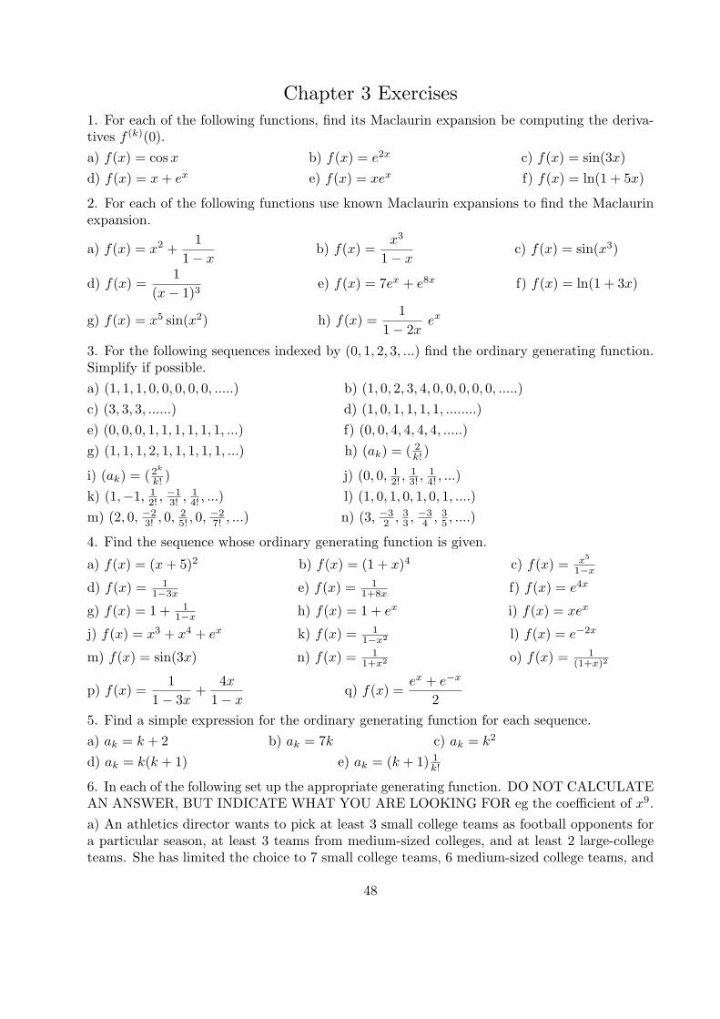
Chapter 3 Exercises1. For each of the following functions, find its Maclaurin expansion be computing the deriva-tives f (k)(0).

a) f(x) = cosx b) f(x) = e2x c) f(x) = sin(3x)

d) f(x) = x+ ex e) f(x) = xex f) f(x) = ln(1 + 5x)

2. For each of the following functions use known Maclaurin expansions to find the Maclaurinexpansion.

a) f(x) = x2 +1

1− xb) f(x) =

x3

1− xc) f(x) = sin(x3)

d) f(x) =1

(x− 1)3e) f(x) = 7ex + e8x f) f(x) = ln(1 + 3x)

g) f(x) = x5 sin(x2) h) f(x) =1

1− 2xex

3. For the following sequences indexed by (0, 1, 2, 3, ...) find the ordinary generating function.Simplify if possible.

a) (1, 1, 1, 0, 0, 0, 0, 0, .....) b) (1, 0, 2, 3, 4, 0, 0, 0, 0, 0, .....)

c) (3, 3, 3, ......) d) (1, 0, 1, 1, 1, 1, ........)

e) (0, 0, 0, 1, 1, 1, 1, 1, 1, ...) f) (0, 0, 4, 4, 4, 4, .....)

g) (1, 1, 1, 2, 1, 1, 1, 1, 1, ...) h) (ak) = ( 2k! )

i) (ak) = ( 2k

k! ) j) (0, 0, 12! ,

13! ,

14! , ...)

k) (1,−1, 12! ,

−13! ,

14! , ...) l) (1, 0, 1, 0, 1, 0, 1, ....)

m) (2, 0, −23! , 0,

25! , 0,

−27! , ...) n) (3, −3

2 , 33 ,

−34 , 3

5 , ....)

4. Find the sequence whose ordinary generating function is given.

a) f(x) = (x+ 5)2 b) f(x) = (1 + x)4 c) f(x) = x5

1−x

d) f(x) = 11−3x e) f(x) = 1

1+8x f) f(x) = e4x

g) f(x) = 1 + 11−x h) f(x) = 1 + ex i) f(x) = xex

j) f(x) = x3 + x4 + ex k) f(x) = 11−x2 l) f(x) = e−2x

m) f(x) = sin(3x) n) f(x) = 11+x2 o) f(x) = 1

(1+x)2

p) f(x) =1

1− 3x+

4x

1− xq) f(x) =

ex + e−x

2

5. Find a simple expression for the ordinary generating function for each sequence.

a) ak = k + 2 b) ak = 7k c) ak = k2

d) ak = k(k + 1) e) ak = (k + 1) 1k!

6. In each of the following set up the appropriate generating function. DO NOT CALCULATEAN ANSWER, BUT INDICATE WHAT YOU ARE LOOKING FOR eg the coefficient of x9.

a) An athletics director wants to pick at least 3 small college teams as football opponents fora particular season, at least 3 teams from medium-sized colleges, and at least 2 large-collegeteams. She has limited the choice to 7 small college teams, 6 medium-sized college teams, and

48

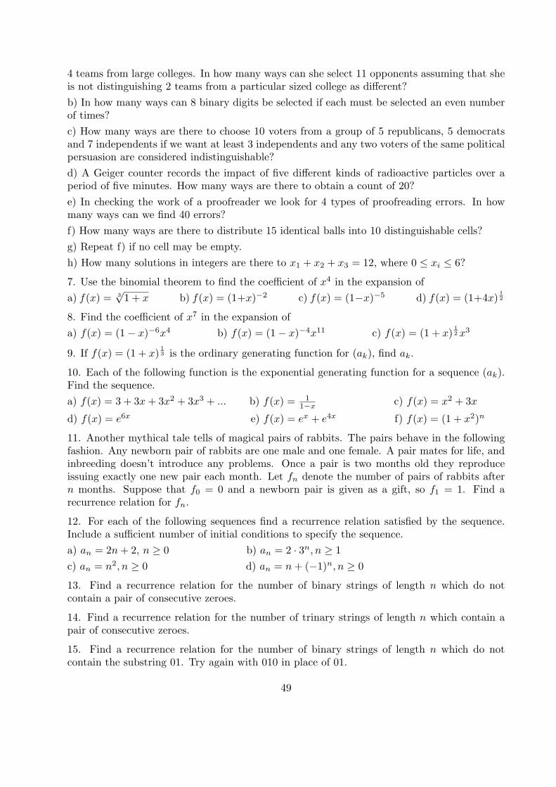
4 teams from large colleges. In how many ways can she select 11 opponents assuming that sheis not distinguishing 2 teams from a particular sized college as different?

b) In how many ways can 8 binary digits be selected if each must be selected an even numberof times?

c) How many ways are there to choose 10 voters from a group of 5 republicans, 5 democratsand 7 independents if we want at least 3 independents and any two voters of the same politicalpersuasion are considered indistinguishable?

d) A Geiger counter records the impact of five different kinds of radioactive particles over aperiod of five minutes. How many ways are there to obtain a count of 20?

e) In checking the work of a proofreader we look for 4 types of proofreading errors. In howmany ways can we find 40 errors?

f) How many ways are there to distribute 15 identical balls into 10 distinguishable cells?

g) Repeat f) if no cell may be empty.

h) How many solutions in integers are there to x1 + x2 + x3 = 12, where 0 ≤ xi ≤ 6?

7. Use the binomial theorem to find the coefficient of x4 in the expansion of

a) f(x) = 3√1 + x b) f(x) = (1+x)−2 c) f(x) = (1−x)−5 d) f(x) = (1+4x)

12

8. Find the coefficient of x7 in the expansion of

a) f(x) = (1− x)−6x4 b) f(x) = (1− x)−4x11 c) f(x) = (1 + x)12x3

9. If f(x) = (1 + x)13 is the ordinary generating function for (ak), find ak.

10. Each of the following function is the exponential generating function for a sequence (ak).Find the sequence.

a) f(x) = 3 + 3x+ 3x2 + 3x3 + ... b) f(x) = 11−x c) f(x) = x2 + 3x

d) f(x) = e6x e) f(x) = ex + e4x f) f(x) = (1 + x2)n

11. Another mythical tale tells of magical pairs of rabbits. The pairs behave in the followingfashion. Any newborn pair of rabbits are one male and one female. A pair mates for life, andinbreeding doesn’t introduce any problems. Once a pair is two months old they reproduceissuing exactly one new pair each month. Let fn denote the number of pairs of rabbits aftern months. Suppose that f0 = 0 and a newborn pair is given as a gift, so f1 = 1. Find arecurrence relation for fn.

12. For each of the following sequences find a recurrence relation satisfied by the sequence.Include a sufficient number of initial conditions to specify the sequence.

a) an = 2n+ 2, n ≥ 0 b) an = 2 · 3n, n ≥ 1

c) an = n2, n ≥ 0 d) an = n+ (−1)n, n ≥ 0

13. Find a recurrence relation for the number of binary strings of length n which do notcontain a pair of consecutive zeroes.

14. Find a recurrence relation for the number of trinary strings of length n which contain apair of consecutive zeroes.

15. Find a recurrence relation for the number of binary strings of length n which do notcontain the substring 01. Try again with 010 in place of 01.

49

16. A codeword over {0, 1, 2} is considered legitimate iff there is an even number of 0’s andan odd number of 1’s. Find simultaneous recurrence relations from which it is possible tocompute the number of legitimate codewords of length n.

17. Suppose that we have stamps of denominations 4,8, and 10 cents each in unlimited supply.Let f(n) be the number of ways to make n cents postage assuming the ordering of the stampsused matters. So a six cent stamp followed by a four cent stamp is different from a four centstamp followed by a six cent stamp. Find a recurrence relation for f(n). Check your recurrenceby computing f(14) and enumerating all possible ways to make fourteen cents postage.

18. Find the characteristic equation of each of the following recurrences.

a) an = 2an−1 − an−2 b) bk = 10bk−1 − 16bk−2

c) cn = 3cn−1 + 12cn−2 − 18cn−3 d) dn = 8dn−4 + 16dn−5

e) ek = ek−2 f) fn+1 = −fn + 2fn−1

g) gn = 15gn−1 + 12gn−2 + 11gn−3 − 33gn−8 h) hn = 4hn−2

i) in = 6in−1 − 11in−2 + 6in−3 j) jn = 2jn−1 + jn−2 − 2jn−3

19. Find the characteristic roots of each recurrence from exercise 18

20. Solve the recurrence relations using the method of characteristic roots.

a) a0 = 1, a1 = 6 and an = 6an−1 − 9an−2, for n ≥ 2.

b) a0 = 3, a1 = 6 and an = an−1 + 6an−2, for n ≥ 2.

c) a2 = 5, a3 = 13 and an = 7an−1 − 10an−2, for n ≥ 4.

d) a0 = 6, a1 = −3 and an = −4an−1 + 5an−2, for n ≥ 2.

e) a0 = 0, a1 = 1 and an = an−1 + an−2, for n ≥ 2.

f) a0 = 2, a1 = 5, a2 = 15, and an = 6an−1 − 11an−2 + 6an−3, for n ≥ 3.

21. Use generating functions to solve each of the recurrences.

a) an = 2an−1 − an−2 + 2n−2, n ≥ 2, where a0 = 3, a1 = 5

b) bk = 10bk−1 − 16bk−2, k ≥ 2, where b0 = 0, and b1 = 1

c) cm = −cm−1 + 2cm−2,m ≥ 2, where c0 = c1 = 1

d) dn = 6dn−1 − 11dn−2 + 6dn−3, whered0 = 0, d1 = 1, and d2 = 2.

22. Find a generating function forCn+1 = 2nCn + 2Cn + 2, n ≥ 0, where C0 = 1. Then findan exponential generating function for the same recurrence.

23. In each case suppose that G(x) is the ordinary generating function for (an). Find an.

a) G(x) =1

(1− 2x)(1− 4x)

b) G(x) =2x+ 1

(1− 3x)(1− 4x)

c) G(x) =x2

(1− 4x)(1− 5x)(1− 6x)

d) G(x) =1

8x2 − 6x+ 1

50

e) G(x) =x

x2 − 3x+ 2

f) G(x) =1

6x3 − 5x2 + x

g) G(x) =2− 3x

(1− x)2(1− 2x)

24. Solve simultaneously the recurrences

an+1 = an + bn + cn, n ≥ 1

bn+1 = 4n − cn, n ≥ 1

cn+1 = 4n − bn, n ≥ 1

subject to a1 = b1 = c1 = 1.

51

Chapter 4: Po′lya Counting

Abstract algebra, or modern algebra, is an area of mathematics where one studies generalalgebraic structures. In contrast the algebra that one studies in, for example, college algebrais very specific and concrete - dealing (almost) exclusively with algebra using real or complexnumber systems.

Basic counting requires only basic algebra. Intermediate counting requires algebra whichis a bit more generalized, namely the formal manipulation of power series. It therefore makessense that advanced counting requires abstract algebra.

The roots of the counting techniques we study are in the work Burnside and Frobenius.George Polya is credited with the most fundamental theorem pertinent to this approach tocounting. Thus this type of counting is named after him.

We start with a large collection of objects. We then decide upon a framework to help usclassify the objects (uniquely) by various types. The goal is to develop a theory to determinethe number of distinct types. The theory we develop uses group theory in deciding whichobjects are of the same type.

We therefore begin with a section devoted to developing the notion of when two objectsare of the same type. This is followed by some basic group theory in the second section. TheFundamental Lemma in section three is often attributed to Burnside. There are argumentsthat it should be attributed elsewhere. We will therefore not specifically attribute it to him.Still if the student should find themselves reading an older text, they’ll recognize the lemmaby the moniker “Burnside’s Lemma”.

§4.1 Equivalence Relations

Given a large set, in order to classify it’s members into distinct types, the classificationscheme must meet certain criteria. First, for any element of the set there should be a class thatthe element fits into. Second, no element should fall into two classes simultaeously. Otherwisewe cannot claim that the types actually classify the elements. Finally, in part because we wantto be able to determine the number of distinct classes, we shall want to require that no classis empty. The point is that we could arbitrarily define classes which will be empty and notreally be counting the number of necessary classes.

For such a classification scheme the distinct classes C1, C2, ..., Cr form a partition of theset A. A partition of a set , A, is a collection of pairwise-disjoint, non-empty subsets, whoseunion is A.

Given a partition of A into the parts C1, C2, ..., Cr we can relate two elements of A whenthey are in the same part. This relation, R ⊆ A×A, has the property that it is reflexive, sinceevery element of A is in some part. R is also symmetric, since if a and b are in the same part,so are b and a. Finally R is transitive since if a and b are in the same part Ci, and b and c arein the same part Cj , then b ∈ Ci ∩ Cj . From the fact that the parts are pairwise disjoint weconclude that Ci = Cj . Whence a and c are in the same part. So a partition of a set definesan equivalence relation on the set.

Conversely given a relation R on A which is an equivalence relation, so it’s simultaneouslyreflexive, symmetric and transitive, we can define the equivalence class of any a ∈ A, denotedby [a], as the set of all elements of A in the relation with a.

Theorem: If R is an equivalence relation on A, and a, b ∈ A, then [a] ∩ [b] = ∅ implies that[a] = [b]

52

Proof: Let c ∈ [a]∩ [b]. Then (a, c), (b, c) ∈ R. Since R is symmetric (a, c), (c, b) ∈ R. BecauseR is transitive we get (a, b) ∈ R. So now if d ∈ [a], we know (b, a) and (a, d) are in R. Therefore(b, d) ∈ R, which is equivalent to d ∈ [b]. Thus [a] ⊆ [b]. The result follows by appealing tosymmetry of argument.

As a corollary we draw that the distinct equivalence classes of an equivalence relationform a partition of the set.

Example: A standard deck of cards contains 52 cards. Each card has a rank 2, 3, 4, 5, 6, 7, 8, 9,10, J = jack,Q = queen, K = king, or A = ace. Each card also has a suit ♡,♠,♣,, or ♢.

So we could choose to classify the cards in a standard deck by considering two cards “thesame” if they had the same suit. In this case there would be four distinct types of objects.

Of course, we might also define two cards to be the same if they were of the same rank.Now there would be thirteen distinct types of objects.

So we sometimes might need to use a subscript [a]R to distinguish the equivalence classof an element a with respect to R as opposed to [a]T which would denote the equivalence classof a with respect to T .

Example: The relation (mod m) on ZZ.

Example: 2-Colorings of C4

§4.2 Permutation Groups

A binary operation on a set S is a function from S × S into S. Standard examples areaddition and multiplication. We will use multiplicative notation. So the image of (g, h) iswritten gh.

A group is a set with a binary operation which is associative, i.e. a(bc) = (ab)c for alla, b, c,∈ G, has identity, i.e. there exists e ∈ G with eg = g = ge for all g ∈ G, and inverses,so for each g ∈ G, there is h, denoted g−1, with gh = e = hg. If in addition the operation iscommutative (ab = ba for all a, b ∈ G) we call the group abelian. Denote the cardinality of Gby |G|. This is called the order of G.

Example: ZZ,+. Here the identity is additive 0 + n = n + 0 = n, and the inverse is too:n+ (−n) = (−n) + n = 0.

Example: IR∗ = IR− {0}, ·. Here we suppress the symbol and use juxtaposition. The identityis 1, and the inverse is the reciprocal.

Notice that in a group we have the cancellation property: ac = ab implies c = b.

Example: Let A be a set and put Sym(A) = {f : A −→ A|f is bijective }. Then Sym(A) isa group with operation being composition of functions. The identity is the identity functionon A, and inverses are inverse functions.

If |A| = |B| = n <∞, there is a bijective function f : A −→ B. Then Sym (A) ∼= Sym (B)where π ∈ Sym (A) corresponds to fπf−1 ∈ Sym (B) one must check the correspondence is 1-1, onto and preserves operations, f is a group isomorphism, which of course behaves somewhatlike a graph isomorphosm. The only difference is graph isomorphisms preserve adjacency andgroup isomorphisms preserve operation.

53

Standardly, if |A| = n, we therefore take A = {1, 2, 3, ..., n} and denote Sym (A) bySn, the symmetric group on n letters. This is a permutation group because its elements aren-permutations of an n-set.

Elements of Sn may be described by two-row tables, T-tables, bipartite graphs, etc.

For computational ease and typesetting efficiency we use cycle notation. (a1a2...al) de-notes the permutation on n letters where ai gets mapped to ai+1, with subscripts computedmodulo l, and where any letter not in {a1, ..., al} is fixed. This is a rather important convention.

Two permutations, π and ρ are disjoint, if π(a) = a implies ρ(a) = a and vice versa.

Theorem: Every nonidentity permutation π ∈ Sn can be written (uniquely up to order) as aproduct of disjoint cycles.

Sketch of proof: The proof uses the second form of mathematical induction, and can becompared to the standard proof of the Fundamental Theorem of Arithmetic. In the inductivestep we pick x with π(x) = x. Form the cycle γ = (x, π(x), π2(x), ..., πl−1(x)) (so l is theleast positive integer with πl(x) = x). If π = γ, we’re done. Otherwise, since γ fixes anyelement of {1, ..., n}−{x, π(x), ..., πl−1(x)}, πγ−1 fixes {x, π(x), ..., πl−1(x)} and can thereforebe considered as an element of Sn−l. Induction kicks in and we’re done.

The order of the cycles is not fixed in the previous theorem because

Fact: If γ and π are disjoint, then γπ = πγ.

Sketch of proof: Check that the two compositions have the same value at each i ∈ {1, 2, ..., n}.There are essentially three cases to consider.

Notice that the converse is not true. Any non-identity permutation will commute with itspowers, but will not be disjoint from them.

A subgroup of a group is a subset which is also a group. We write H ≤ G to mean H isa subgroup of G.

Theorem: Let ∅ = H ⊆ G, where G is a group. H is a subgroup iff ab−1 ∈ H for all a, b ∈ H.

Proof: The forward implication is trivial.For the converse, since H = ∅, there is a ∈ H. Hence e = aa−1 ∈ H. And if b ∈ H,

b−1 = eb−1 ∈ H. H inherits associativity from G.

Theorem: Let ∅ = H ⊆ G, where G is a group and #H = n <∞. H is a subgroup iff ab ∈ Hfor all a, b ∈ H.

Proof: The forward implication is trivial.Let a ∈ H. Among the elements a, a2, a3, ..., an, an+1, all must be in H by closure. Since

|H| = n, these elements cannot all be distinct. Therefore there exists superscripts i and j withj > i so that aj = ai. Therefore aj−i = e ∈ H. In fact we see that a−1 = aj−i−1. So fora, b ∈ H, a, b−1 ∈ H. By closure ab−1 ∈ H. And we’re done by the previous theorem.

Notice that a cycle γ of length l satisifies that l is the smallest positive integer for whichγl = id. We say the the cycle has order l, since the set of distinct powers of {id = γ0, γ, ....γl−1}is a group or order l, since it satisfies the previous theorem. We write ⟨γ⟩ for this group.

54

Example: < (1234) >= {id, (1234), (13)(24), (1432)}. Notice that a cycle’s order is the sameas its length.

For general permutations we have that when γπ = πγ, by induction (γπ)n = γnπn.Together with the fact that the order (as a group element) of an l-cycle is l when γ and πcommute o(γπ) = lcm(o(γ), o(π)). Thus if we write a permutation as a product of disjointcycles, we can easily compute its order.

When π is the product of disjoint cycles which includes exactly ea cycles of length a > 2,

we define the type of π to be type (π) =∏a

aea , and extend to the identity by saying the

identity has type 1. The order of π as a group element is the least common multiple of lengthsa, where ea > 0.

§4.3 Group Actions

If S is a set and G is a group, G acts on S if there is a map ∗ : G× S −→ S so that1) g1 ∗ (g2 ∗ s) = (g1g2) ∗ s and 2) e ∗ s = s for all s ∈ S.

Example: Every group acts on itself by left multiplication.

Remark: We sometimes will find it useful to use functional notation for a group action. Soinstead of writing g ∗ s we will write g(s).

If G acts on S define the relation ∼ on S by x ∼ y iff there exists g ∈ G with g ∗ x = y.

Theorem: ∼ is an equivalence relation on G.

Proof: 1) For s ∈ S, s ∼ s since e ∗ s = s. Therefore ∼ is reflexive.2) If x ∼ y, there is g ∈ G so that g ∗ x = y. Then g−1 ∗ y = g−1 ∗ (g ∗ x) = (g−1g) ∗ x =

e ∗ x = x, so y ∼ x. Therefore ∼ is symmetric.3) If x ∼ y and y ∼ z, then there are g, h ∈ G with g ∗ x = y, and h ∗ y = z. So

(hg) ∗ x = h ∗ (g ∗ x) = h ∗ y = z. Hence ∼ is transitive.

Example: ⟨(1234)⟩ acts on the 2-colored C4’s.

Example: {id, reverse} acts on the set of open necklaces of length k.

General example: G a group acts on itself by conjugation g ∗h = ghg−1. Here the equivalenceclasses are the conjugacy classes.

For x ∈ S, the orbit of x under G is denoted G ∗ x = {g ∗ x|g ∈ G}. Also Gx = {g ∈G|g ∗ x = x} is the stabilizer of x in G.

Fact: Gx ≤ G. (the proof is straightforward)

Theorem: |G| = |G ∗ a| · |Ga|.

Proof: Suppose that G ∗ a = {b1, ..., br}, where the bi’s are all distinct. Then there is anr-subset P = {π1, π2, ..., πr} of G with πi ∗ a = bi, for i = 1, 2, ..., r (the π’s are distinct sinceπ ∗ a is unique).

Now for γ ∈ G, if γ ∗ a = bk = πk ∗ a, then π−1k ∗ γ ∗ a = a. So π−1

k γ ∈ Ga. Sayπ−1k γ = σ ∈ Ga. Then γ = idγ = (πkπ

−1k )γ = πk(π

−1k γ) = πkσ. So every element of G can be

written as something in P times something in Ga. Therefore |G| ≤ |P ||Ga| = |G ∗ a||Ga|.

55

To show equality suppose that γ = πkσ = πmτ , where πk, πm ∈ P and σ, τ ∈ Ga. Thusπkσ ∗ a = πk ∗ a = bk, while πmτ ∗ a = πm ∗ a = bm. So bk = bm, and thus πk = πm. Thus bythe cancellation property of a group σ = τ .

When G is finite, the theorem gives a useful divisibility condition.

General Example: If H ≤ G, for any g ∈ G, gH = {gh|h ∈ H} is the left coset of H in Glabelled by g. The group G acts on S = {gH|g ∈ G}, the set of left cosets of H in G, by leftmultiplication i.e. g ∗ xH = gxH. In this case GH = H (i.e. aH = H iff a ∈ H, and generallyaH = bH iff ab−1 ∈ H). We denote the number of distinct left cosets of H in G by [G : H]and call it the index of H in G. The previous theorem says that |G| = |H| · [G : H], which isLagrange’s Theorem.

If G acts on S and there is s ∈ S so that G ∗ s = S, then G acts transitively on S. In theprevious general example G acts transitively on the left cosets of H by left multiplication. Ithappens that G also acts transitively on the right cosets of H in G, by g ∗Hk = Hkg. So thetheorem allows us to deduce that the number of distinct right cosets of H in G is the same asthe number of distinct left cosets of H in G.

When H ≤ G sometimes the set of left cosets is different from the set of right cosets. Forexample the cosets of ⟨(12)⟩ in S3. However sometimes the set of left cosets is the same as theset if right cosets, i.e. gH = Hg for all g ∈ G. We call such a subgroup normal, and writeN△G.

The condition that gN = Ng means that for every n ∈ N , gn ∈ Ng. Therefore thereexists n′ ∈ N with gn = n′g. So gN = Ng iff for all n ∈ N, gng−1 = n′ ∈ N iff gNg−1 = Nfor all g ∈ G.

If N△G and n ∈ N , then Cn the conjugacy class of n must be in N . Therefore N△Gimplies that N is a union of conjugacy classes. So computing the conjugacy classes of G canfacilitate finding normal subgroups of G.

By generalizing the example of ⟨(123)⟩△S3 we conclude that if [G : H] = 2, then H△G.

An element a ∈ A is invariant under π ∈ G if π ∗ a = a.

Example: The four bead necklace with all beads white is invariant under (1234).

For a permutation π we define Inv(π) = |{a ∈ A|π ∗ a = a}|. So Inv(π) is the numberof elements in A which π leaves invariant. We call the set {a ∈ A|π ∗ a = a} = Fix (π). SoInv(π) is the size of Fix(π). We also say that π ∈ G stabilizes a, if π ∗ a = a.

THE LEMMA: Let S be the equivalence relation on A induced by the action of a group G.Then the number of distinct equivalence classes is 1

|G|∑

π∈G Inv(π).

Proof: Let F = {(π, x) ∈ G × A|π ∗ x = x}. Define 1I(g, x) to be 1 if (π, x) ∈ F , and 0otherwise. Finally let S = {G ∗ x1, G ∗ x2, ..., G ∗ xr} be the distinct orbits of A under G.

|F | =∑x∈A

∑π∈G

1I(π, x) =∑x∈A

|Gx|

=∑π∈G

∑x∈A

1I(π, x) =∑π∈G

|Fix(π)| =∑π∈G

Inv (π)

56

Hence1

|G|∑π∈G

Inv(π) =1

|G|∑x∈A

|Gx| =∑x∈A

|Gx||G|

=∑x∈A

|Gx||G ∗ x||Gx|

=∑x∈A

1

|G ∗ x|

=r∑

i=1

∑x∈G∗xi

1

|G ∗ xi|

=r∑

i=1

[1

t+

1

t+ ...+

1

t

], t terms

=

r∑i=1

1 = r = |S|

So the number of orbits is the average of the fix set sizes.

Example: There are six equivalence classes when ⟨(1234)⟩ acts on the 2-colored necklaces with4 beads.

§4.4 Colorings

Let D be a set. A coloring of D is an assignment of a color to each element of D. That isa coloring corresponds to a function f : D −→ R, where R is a set of colors. When |D| = k,and |R| = m, there are mk colorings of D using the colors from R.

Let C(D,R) denote the set of all colorings of D using the colors from R.If G is a permutation group on D and π ∈ G, then there is a corresponding permutation

π∗ of C(D,R). If f is a coloring, then π∗(f) is another coloring where π∗f(d) = f(π(d)), forall d in D.

As will be seen in our examples, we might also define this more naturally as π∗f(d) =f(π−1(d)), for all d ∈ D. The point is that in our fundamental lemma, we are summing overall group elements - which is equivalent to summing over all of the inverses of group elements.

Example: Label the vertices of a 4-cycle clockwise 1,2,3, and 4. Color these Red, Blue, Yellowand Green. We can think of f as the output string RBYG. Let π = (1234). Then π∗fhasoutput string BYGR.

As an obvious fact we have

Fact: The set of induced permutations G∗ = {π∗|π ∈ G} is a group under composition offunctions, and |G∗| = |G|.

More to the point is the following fact.

Fact: If G induces an equivalence relation S on D, then G∗ induces an equivalence relationS∗ on C(D,R) by fS∗g iff there exists π ∈ G with g = π∗f .

The proof is left to the reader. Notice here that g = π∗f iff f = (π−1)∗g. So our previousremark is well-founded.

57

The point is that we may concentrate on D and groups acting on D, since really all thatis important about R is its cardinality.

§4.5 The Cycle Index and the Pattern Inventory

When π ∈ Sn is written as a product of disjoint cycles, the result is called its cycledecomposition. We will write cd(π) for the cycle decomposition of π. Given π we can order

the terms of cd(π) with all the 1-cycles first, followed by any 2-cycles, etc. So π =

l∏i=1

ei∏j=1

γi,j ,

where γi,j is a cycle of length i and there are ei cycles of length i appearing.

Next we define type(π) =l∏

i=1

iei . Notice thatl∑

i=1

iei = n. Also we define cyc(π) =l∑

i=1

ei

which is the number of cycles in cd(π).

Example: (1234)(56)(78) ∈ S8 has type 2241 and cyc((1234)(56)(78)) = 3.

Theorem: (Polya Version 1) Suppose that G is a group acting on D. Let R be an m-setof colors. Then the number of distinct colorings in C(D,R) which is the number of distinct

equivalence classes for S∗ induced by G on C(D,R) equals1

|G|∑π∈G

mcyc(π).

Proof: By the fundamental lemma it suffices to show that mcyc(π) = Inv(π∗) for all π ∈ G.But any element of C(D,R) is left invariant under π∗ iff all elements of D in a cycle of πare colored the same color. So for each cycle in cd(π) we have m choices for color. Themultiplication principle now gives the result.

So as promised the induced group G∗, and anything about the set of colors R, except itssize, are immaterial.

If G is a permutation group where k is the length of the longest cycle occuring in the cycledecomposition of any element of G, the cycle index of G is defined as

PG[x1, x2, ..., xk] =1

|G|∑π∈G

( ∏a≥1

xeaa

)

where the exponents in the products come from the cycle decompositions of the correspondingpermutations.

Example: G = ⟨(1234)⟩ consists of {(1)(2)(3)(4), (1234), (13)(24), (1432)}. So

PG(x1, x2, x3, x4) =1

4[x4

1 + x22 + 2x4].

Notice that PG(m,m,m,m) =1

4[m4 +m2 + 2m] =

1

|G|∑π∈G

mcyc(π).

A weight function w : R −→ S, is any function from a set, R, of colors into the set S.

58

Theorem: (Polya Version 2) If a group G acts on a set D whose elements are colored byelements of R, which are weighted by w, then the expression

PG

[∑r∈R

w(r),∑r∈R

(w(r)2), ...,∑r∈R

(w(r)k)

]

generates the pattern inventory of distinct colorings by weight, where PG[x1, x2, ..., xk] is thecycle index of G.

Proof: See appendix 1.

Most especially the constant function w(r) = 1 for all r ∈ R gives the number of distinctcolorings.

By singling out a particular color, say w(r) = 1 for r = b, and w(b) = b = 1. we cangenerate the distinct colorings enumerated by how many times the color b is used.

59

Chapter 4 Exercises1. In each case determine whether S is an equivalence relation on A. If it is not, determinewhich properties of an equivalence relation fail to hold.

a) A is the power set of {1, 2, 3, ..., n}, aSb iff a and b have the same number of elements.

b) A is the power set of {1, 2, 3, ..., n}, aSb iff a and b are disjoint.

c) A is all people in Grand Forks, aSb iff a and b have the same blood type.

d) A is all people in North Dakota, aSb iff a and b live within 10 miles of each other.

e) A is all bit strings of length 10, aSb iff a and b have the same number of ones.

2. For each equivalence relation from exercise 1, identify all equivalence classes.

3. In each case find π1 ◦ π2

a) π1 =

(1 2 3 44 3 2 1

), π2 =

(1 2 3 42 3 1 4

)b) π1 =

(1 2 3 42 1 4 3

), π2 =

(1 2 3 44 3 1 2

)c) π1 =

(1 2 3 4 51 3 2 4 5

), π2 =

(1 2 3 4 52 1 3 5 4

)d) π1 =

(1 2 3 4 5 66 1 5 2 4 3

), π2 =

(1 2 3 4 5 62 3 4 5 6 1

)4. In each case determine if ◦ is a binary operation on X. If it is, determine which of the threegroup axioms hold for X, ◦.

a) X =

{(1 2 3 4 51 2 3 4 5

),

(1 2 3 4 55 4 3 2 1

)}, where ◦ is composition of functions.

b) X = Q, ◦ is addition.c) X = Q, ◦ is multiplication.

d) X = IN, ◦ is addition.e) X = IR− {0}, ◦ is multiplication.

f) X is all 2× 2 matrices with real entries, ◦ is matrix multiplication.

5. In each case the group G induces an equivalence relation on the set A, find all of the distinctequivalence classes.

a) A = {1, 2, 3, 4, 5}, G =

{(1 2 3 4 51 2 3 4 5

),

(1 2 3 4 55 2 3 4 1

)}, ◦ is composition.

b) A = {1, 2, 3, 4, 5, 6}, G =

{(1 2 3 4 5 61 2 3 4 5 6

),

(1 2 3 4 5 62 1 3 4 5 6

),(

1 2 3 4 5 61 2 4 3 5 6

),

(1 2 3 4 5 61 2 3 4 6 5

),

(1 2 3 4 5 62 1 4 3 5 6

),(

1 2 3 4 5 62 1 3 4 6 5

),

(1 2 3 4 5 61 2 4 3 6 5

),

(1 2 3 4 5 62 1 4 3 6 5

)}, ◦ is composition.

c) A = {1, 2, 3, 4, 5}, G =

{(1 2 3 4 51 2 3 4 5

),

(1 2 3 4 52 3 4 5 1

),

(1 2 3 4 53 4 5 1 2

),(

1 2 3 4 54 5 1 2 3

),

(1 2 3 4 55 1 2 3 4

)}, ◦ is composition.

60

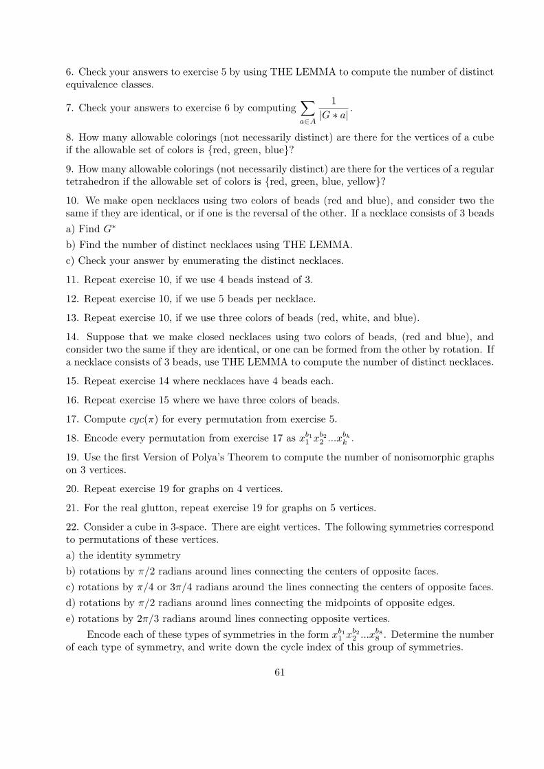
6. Check your answers to exercise 5 by using THE LEMMA to compute the number of distinctequivalence classes.

7. Check your answers to exercise 6 by computing∑a∈A

1

|G ∗ a|.

8. How many allowable colorings (not necessarily distinct) are there for the vertices of a cubeif the allowable set of colors is {red, green, blue}?

9. How many allowable colorings (not necessarily distinct) are there for the vertices of a regulartetrahedron if the allowable set of colors is {red, green, blue, yellow}?

10. We make open necklaces using two colors of beads (red and blue), and consider two thesame if they are identical, or if one is the reversal of the other. If a necklace consists of 3 beads

a) Find G∗

b) Find the number of distinct necklaces using THE LEMMA.

c) Check your answer by enumerating the distinct necklaces.

11. Repeat exercise 10, if we use 4 beads instead of 3.

12. Repeat exercise 10, if we use 5 beads per necklace.

13. Repeat exercise 10, if we use three colors of beads (red, white, and blue).

14. Suppose that we make closed necklaces using two colors of beads, (red and blue), andconsider two the same if they are identical, or one can be formed from the other by rotation. Ifa necklace consists of 3 beads, use THE LEMMA to compute the number of distinct necklaces.

15. Repeat exercise 14 where necklaces have 4 beads each.

16. Repeat exercise 15 where we have three colors of beads.

17. Compute cyc(π) for every permutation from exercise 5.

18. Encode every permutation from exercise 17 as xb11 xb2

2 ...xbkk .

19. Use the first Version of Polya’s Theorem to compute the number of nonisomorphic graphson 3 vertices.

20. Repeat exercise 19 for graphs on 4 vertices.

21. For the real glutton, repeat exercise 19 for graphs on 5 vertices.

22. Consider a cube in 3-space. There are eight vertices. The following symmetries correspondto permutations of these vertices.

a) the identity symmetry

b) rotations by π/2 radians around lines connecting the centers of opposite faces.

c) rotations by π/4 or 3π/4 radians around the lines connecting the centers of opposite faces.

d) rotations by π/2 radians around lines connecting the midpoints of opposite edges.

e) rotations by 2π/3 radians around lines connecting opposite vertices.

Encode each of these types of symmetries in the form xb11 xb2

2 ...xb88 . Determine the number

of each type of symmetry, and write down the cycle index of this group of symmetries.

61

23. The number of permutations of {1, 2, ..., n} with code xb11 xb2

2 ...xbnn is given by

n!

b1!b2!...bn!1b12b23b3 ...nbn

Verify this formula for n = 5, b1 = 1, b2 = 2, b3 = b4 = b5 = 0 by enumerating allpermutations of the proper type.

24. How many open four bead necklaces are there in which each bead is one of the colors b, r,or p, there is at least one p, and two necklaces are considered the same if they are identical orif one is the reversal of the other.

25. Repeat exercise 24 if the necklaces are closed and two are considered the same if one is arotation of the other.

26. Repeat exercise 24 if the necklaces are closed and two are considered the same if one is arotation, or a reflection of the other.

62

Chapter 5: Combinatorial Designs

This chapter begins our foray into the realm governed by the existence question. Givencertain conditions, can we find a configuration of finite sets which meet the conditions? Ifwe cannot, we wish to prove so. If we can, we’d like to be able to demonstrate that theconfiguration satisfies the conditions. If possible, we might even want to classify all possibleconfigurations which meet the requirements.

For non-existence proofs, we will not necessarily need the power of abstract algebra. Forconstructions, and to aid in discussing classification we will. So in this chapter we start withtwo sections dedicated to finite fields.

This is followed by a section on the most basic configurations we will consider, Latinsquares. The initial motivation for considering these configurations was to remove possibleambiguities which might negatively affect the collection of data from agricultural experiments.

The third section is devoted to introducing so-called balanced incomplete block designs,which were also used in the design of experiments.

In the last two sections we give some basic construction techniques for balanced incompleteblock designs, and discuss connections with the classification of finite simple groups.

§5.1 Finite Prime Fields

Recall that ZZ denotes the integers, aka whole numbers. With respect to the operationsof addition and multiplication the integers satisfy the following algebraic axioms:

1) and 5) Addition and Multiplication are associative, eg. (ab)c = abc = a(bc) always.

2) and 6) Addition and Multiplication are commutative, eg. a+ b = b+ a always.

3) and 7) There is an additive identity (0) and a multiplicative identity (1).

4) Every element has an additive inverse.

8) Multiplication distributes over addition.

The function mod n : ZZ −→ {0, 1, 2, 3, ..., n− 1} := ZZn takes as input any whole numbera and outputs r, where a = qn + r, and 0 ≤ r < n. We can use this to define and additionand a multiplication on ZZn where a+n b = (a+ b)mod n, and a×n b = (a× b)mod n.

Technically we’re operating on the equivalence classes modulo n. So [a]+n [b] = [a+b], and[a] ×n [b] = [ab], where the convention is that we always use the standard system of distinctrepresentatives for equivalence classes {[0], [1], [2], ...[n − 1]}. However the equivalence classnotation is a little cumbersome, so we”ll dispense with the technicalities to save ourselves alittle grief. Also when the context is clear we’ll drop the subscipts on the operations.

With these definitions ZZn = {0, 1, 2, ..., n− 1},+n,×n also satisfies axioms 1-8 by inheri-tance and the fact that mod n is a function.

Definition A (commutative) ring is a set R with operations addition and multiplicationwhich satisfies axioms 1)-8).

Definition A field is a set IF with operations addition and multiplication which satisfyaxioms 1-8 above, has 1 = 0 and which satisfies the further axiom

9) Every nonzero element has a multiplicative inverse.

63

Equivalently IF∗ := IF− {0} is a group under multiplication.

Note that the integers do not form a field since, for example, 2−1 = 12 /∈ ZZ.

Fact: If IF is a field and a = 0, then ab = ac implies b = c.

Proof: Since a = 0, a−1 ∈ IF. Thus ab = ac means a−1ab = a−1ac. Whence b = c.

Fact: If IF is a field and ab = 0, then a = 0, or b = 0.

Proof: If a = 0 and ab = 0, then b = a−1ab = a−10 = 0.

Corollary If R is a set with addition and multiplication satisfying axioms 1− 5, 7 and 8 andthere are nonzero elements a, b ∈ R with ab = 0, then R is not a field.

Theorem: Let n > 1 be an integer. ZZn is a field iff n is prime.

Proof: For the reverse implication it suffices to show that every nonzero element has a mul-tiplicative inverse. So let a ∈ ZZn − {0}, where n is prime. Because n is prime gcd(a, n) = 1.There are therefore integers s and t so that as+ tn = 1. Therefore a×n s = 1.

Conversely, since n > 1, if n is not prime, then it is composite. Therefore there existintegers a, b with 1 < a, b < n and n = ab. Therefore a×n b = 0. Therefore ZZn is not a fieldby the corollary above.

Fact: If a, b ∈ IF a field and a = 0, then there is a unique solution in IF to ax = b, namelyx = a−1b.

Corollary: If a ∈ IF− {0}, where IF is a field, then a−1 is unique.

Fact: If IF is a field then x2 − 1 = 0 has at most 2 solutions in IF.

Proof: In any field x2 − 1 = (x − 1)(x + 1), so if x2 − 1 = 0, either x + 1 = 0 or x − 1 = 0.Since 1 = −1 in ZZ2 these solutions do not need to be distinct.

Corollary: For p an odd prime ZZp − {−1, 0, 1} is the disjoint union of p−32 sets of the form

{a, a−1}.Proof: Any a ∈ ZZp − {−1, 0, 1} has a unique multiplicative inverse. a−1 satisfies that(a−1)−1 = a. Finally a = a−1 is equivalent to a2 = 1. Which is equivalent to a being asolution to x2 − 1 = 0.

Wilson’s Theorem: If p is prime, then (p− 1)! ≡ −1(mod p).

Proof: The theorem is trivial for p = 2 so suppose that p is an odd prime. Let I be a subsetof ZZp so that {1} ∪ {−1} ∪a∈I {a, a−1} is a partition of ZZ∗

p. Then

(p− 1)! = (p− 1)(p− 2)... · 2 · 1 ≡ −1 · 1 ·∏a∈I

aa−1 ≡ −1 · 1 · 1p−32 ≡ −1(mod p)

Fact: If a ∈ ZZ∗p, then for each k ∈ ZZ∗

p there is a unique j ∈ ZZ∗p with ak ≡ j(mod p).

Proof: If ak ≡ al(mod p), then multiplying both sides by a−1 gives k ≡ l(mod p)

64

Fermat’s Little Theorem: If p is prime and p | a, then ap−1 ≡ 1(mod p).

Proof: WLOG p = 2. Now a · 2a · 3a · ... · (p− 1)a ≡ 1 · 2 · 3 · ... · (p− 1)(mod p) by the previousfact after rearranging terms. We rewrite this as ap−1[(p− 1)!] ≡ (p− 1)!(mod p). We deducethe conclusion by cancelling −1 ≡ (p− 1)!(mod p) from both sides.

Definition: For integers n, a ordna is the least positive integer k so that ak ≡ 1(mod n).Notice that ordna exists only when gcd(a, n) = 1

Theorem: am ≡ 1(mod n) iff k = ordna|m.

Proof: (=⇒) If am ≡ 1(mod n) there are unique integers q, r with m = kq+ r and 0 ≤ r < k.Now 1 ≡ am ≡ akq+r ≡ akqar ≡ (ak)qar ≡ 1qar ≡ ar(mod n). By the minimality of k wemust have r = 0.(⇐=) If k|m, then m = kq for some q ∈ ZZ. Thus am = akq ≡ (ak)q ≡ 1q ≡ 1(mod n)

Corollary: If p is prime ordpa|(p− 1) for all a ∈ ZZ∗p.

Definition: An integer a is a primitive root modulo a prime p if ordpa = p− 1.

Theorem:(Lagrange) If p is a prime integer and f is a polynomial with integral coefficientsof degree n and p does not divide f ’s lead coefficient, then f(x) ≡ 0(mod p) has at most nincongruent solutions mod p.

Proof: We use induction on n. If f(x) = a1x + a0 where p |a1 then f(x) ≡ 0(mod p) isequivalent to a1x ≡ −a0(mod p). We are done by previous theorems. So suppose that thetheorem is true for all polynomials with integral coefficients of degree less than or equal to n−1for which p does not divide the lead coefficient. Let f(x) = anx

n + an−1xn−1 + ..+ a1x+ a0,

where p | an.If f(x) ≡ 0(mod p) has no solutions, then we’re done.Else if a is a solution write f(x) = (x − a)q(x) + r(x), where r(x) = 0, or the degree of

r(x) is less than the degree of x − a (which is one). Thus r is a constant polynomial. Noticethat the degree of q(x) = n− 1.

Now f(a) = (a− a)q(a) + r = r ≡ 0(mod p). So f(x) ≡ (x− a)q(x)(mod p).So if b is another solution to f(x) ≡ 0(mod p), then either (b − a) ≡ 0(mod p) or q(b) ≡

0(mod p). Thus any solution b ≡ a(mod p) is a solution to q(x) ≡ 0(mod p). We are now doneby inductive hypothesis.

Theorem: Let p be prime and d a positive divisor of p− 1. xd − 1 ≡ 0(mod p) has exactly dincongruent solutions modulo p.

Proof: Since d|(p− 1), there is an integer e with p− 1 = de. So xp−1− 1 = (xd− 1)(xd(e−1)+xd(e−2)+ ...+xd+1). Call the second polynomial q(x). By Fermat’s Little Theorem xp−1−1 ≡0(mod p) has exactly p− 1 incongruent solutions modulo p. Each of these is either a solutionof xd − 1 ≡ 0(mod p), or q(x) ≡ 0(mod p).

By Lagrange’s Theorem the number of incongruent solutions to xd− 1 ≡ 0(mod p) is lessthan or equal to d. Also the number of incongruent solutions to q(x) ≡ 0(mod p) is less thanor equal to (p− 1)− d = d(e− 1) = deg(q(x)). Therefore the number of incongruent solutionsto xd − 1 ≡ 0(mod p) is at least (p− 1)− [(p− 1)− d] = d. Thus the number of incongruentsolutions to xd − 1 ≡ 0(mod p) is exactly d.

65

Euler’s φ-function counts the number of positive whole numbers not greater than a given onewhich are also relatively prime to it.

Theorem: Let p be prime and d be a positive divisor of p− 1, there are exactly φ(d) incon-gruent integers with order d modulo p.

Proof: First we need a lemma due to K.F. Gauss.

Lemma: For a positive integer n,∑d|nd>0

φ(d) = n

Proof of lemma: Let d|n, d > 0 and Sd = {m ∈ ZZ|1 ≤ m ≤ n and gcd(m,n) = d}. Recallthat gcd(m,n) = d iff gcd(md ,

nd ) = 1. Thus |Sd| = φ(nd ).

Every integer m with 1 ≤ m ≤ n is in exactly one set Sd where d is a positive divisor of

n, therefore∑d|nd>0

φ(n

d) = n.

But since d|n and d > 0, n = dk, for some positive integer k which is also a divisor of n.

Therefore∑d|nd>0

φ(n

d) =

∑k|nk>0

φ(k) = n.

Now if we let f(d) denote the number of integers between 1 and p−1 inclusive which have

order d modulo p we have p− 1 =∑

d|(p−1)d>0

f(d) =∑

d|(p−1)d>0

φ(d).

To show f(d) = φ(d) for all positive divisors d of p− 1 it suffices to show f(d) ≤ φ(d) forall positive divisors d of p− 1, since we could not have strict inequality anywhere.

So if f(d) = 0 for some positive divisor d of p− 1, we are done since φ(d) > 0 for d > 0.Else f(d) > 0 and there is a ∈ ZZ∗

p with ordpa = d. The definition of order implies

that a, a2, ..., ad are all incongruent (else ordpa < d). Finally for 1 ≤ j ≤ d (aj)d ≡ ajd ≡adj ≡ (ad)j ≡ 1j ≡ 1(mod p). So the d powers of a above are all d incongruent solutions toxd − 1 ≡ 0(mod p).

The proof of the theorem is completed by the following lemma and corollary.

Lemma: For i ∈ ZZ ordn(ai) =

ordna

gcd(ordna, i).

Proof: Put d = gcd(ordna, i) and k = ordna. Write k = db and i = dc where b, c ∈ ZZ. Notice

that gcd(b, c) = 1 and b =k

d=

ordna

gcd(ordna, i).

Now (ai)b ≡ (adc)b ≡ abcd ≡ (abd)c ≡ (ak)c ≡ 1c ≡ 1(mod n). Therefore ordn(ai)|b.

Also ai·ordn(ai) ≡ (ai)ordna

i ≡ 1(mod n), so k|i · ordn(ai). Which is to say that db|dc ·ordn(a

i). Therefore b|c · ordn(ai). Since gcd(b, c) = 1 we have b|ordn(ai).Since b|ordn(ai) and vice versa, and they are both positive integers, they are equal.

Corollary: ordn(ai) = ordna iff gcd(ordna, i) = 1.

The theorem has now been proved.

Corollary: (Primitive Root Theorem) There are exactly φ(p−1) incongruent primitive rootsmodulo a prime p.

We wish to generalize the above set of theorems to a larger class of objects. So far whatwe have done is prove a body of theorems for the so-called finite prime fields, which are those

66

which have a prime number of elements. In general we can construct a finite field of orderq = pn for any prime p and positive integer n.

§5.2 Finite Fields

To begin with the characteristic of a ring (or field) is zero if m · 1 = 0 implies m = 0,otherwise it is the least positive integer m so that m · 1 = 1+ 1+ ...+ 1 = 0 in the ring.

Theorem: If IF is a finite field then its characteristic is prime, and IF contains a subfieldisomorphic to ZZp.

Proof: Let 1 ∈ IF, and n = |IF|. Then 1, 2 · 1, ..., (n + 1) · 1 are not all distinct. Thereforethere are positive integers i and j with i < j and i ·1 = j ·1. Thus (j− i) ·1 = 0 with j− i > 0.Thus a finite field does not have characteristic zero.

Let m be the characteristic of IF. So IF0 = {1, 2 · 1, 3 · 1, ....,m · 1 = 0} are all distinctin IF (if not, m is not be the least positive integer with m · 1 = 0). Notice that IF0 is closedunder addition and multiplication. Also IF0 satisfies the field axioms by inheritance from IF.Therefore IF0 is a subfield of IF.

Define a ring homomorphism (preserves + and ·) from IF0 to ZZm by f(k · 1) = k. Sincef is clearly bijective and preserves operations, ZZm must be a field. Thus m is prime and weare done.

Corollary: If IF is a finite field with characteristic p, then p · x = 0 for all x ∈ IF.

Proof: p · x = x+ x+ ...+ x = x(1+ 1+ ...+ 1) = x · p · 1 = x · 0 = 0

Corollary: If IF is a finite field with q elements and characteristic p, then q = pn for somen ∈ IN.

Proof: Since IF is finite we can form a set S = {x1, x2, ..., xn} with a minimal number ofelements so that every element x ∈ IF is a linear combination a1x1 + a2x2 + ...+ anxn, wherea1, a2, ..., an ∈ ZZp (from the previous corollary). No element of S can be written as a linearcombination of the others, or else S does not have a minimal number of elements.

For some x ∈ IF suppose that x = a1x1+a2x2+ ...+anxn and x = b1x1+b2x2+ ...+bnxn

where ai, bi ∈ ZZp. Suppose that there exists i so that aj = bj for all j > i, but ai = bi. Then0 = (a1− b1)x1 +(a2− b2)x2 + ...+(ai− bi)xi, with c = ai− bi = 0 ∈ ZZp. Put d = c−1 in ZZp.Then xi = −d[(a1 − b1)x1 + (a2 − b2)x2 + ...+ (ai−1 − bi−1)xi−1] a contradiction. Thus everyx ∈ IF is writable in exactly one way as a ZZp-linear combination of the xk’s. Every ZZp-linearcombination of elements in S is in IF because IF is closed under addition. We therefore havethat |IF| = pn.

In order to construct finite fields of order pn where p is prime and n > 1 we must firstconsider polynomials.

A natural power function is of the form xm where m ∈ IN = {0, 1, 2, ...}. For a ring, R, apolynomial over R is an R-linear combination of a finite number of natural power functions.For a nonzero polynomial the largest natural number n for which the coefficient of xn is nonzerois the degree of the polynomial. When a polynomial of degree n has 1 as the coefficient on xn

it is called a monic polynomial. The degree of the zero polynomial is not really defined, butcan be taken to be −1 or even −∞. The set of all polynomials over R is denoted R[x]. Wemay add two polynomials by adding the respective coefficients and multiply polynomials byconvoluting the coefficients.

67

Fact: R[x] is a ring with respect to the addition and multiplication described above. MoreoverR[x] is commutative if R is.

Proof: Omitted for esthetic reasons.

When the ring of coefficients R is a field special things happen. For example

Theorem: (The Division Algorithm for Polynomials) If IF is a field, f, g ∈ IF[x] and g = 0then there are unique polynomials q and r so that f = qg + r and either r = 0 or the degreeof r is strictly less than the degree of g.

Proof: Use induction on the degree of f .

We write g|f and say g divides f exactly when r = 0 from the division algorithm.

If c ∈ IF and f(x) =

n∑k=0

aixi, then f(c) =

n∑k=0

aici is the value of f at c. We say that c is

a root of f when f(c) = 0.

Theorem: (Factor Theorem) If f ∈ IF[x]−{0}, where IF is a field, then f(c) = 0 iff (x−c)|f(x).Proof: By the division algorithm f(x) =! q(x)(x − c) + r(x) where r(x) is zero or has degreeless than 1. In any case r(x) is a constant k ∈ IF. When we evaluate at c = 0 we find f(c) = k.Thus f(c) = 0 iff r = 0.

As a corollary (provable by induction) we have

Theorem: (Lagrange again) If IF is a field and f(x) ∈ IF[x] has degree n, then f has at mostn roots in IF.

We are mostly interested in the extreme behavior with respect to the previous theorem.For example one can show that x2 + x+ 1 has no roots in ZZ2[x]. On the other hand when pis prime xp − x has p distinct roots in ZZp[x] by Fermat’s Little Theorem. When a polynomialf of degree n has exactly n distinct roots in IF we say that IF splits f , or that f splits in IF.

A polynomial f ∈ IF[x] is irreducible over IF if f = gh implies either g ∈ IF or h ∈ IF.Notice that an irreducible polynomial has no roots in IF. The converse is false as demonstratedby x4 + x3 + x+ 2 = (x2 + x+ 2)(x2 + 1) in ZZ3[x]. However the following lemma is true

Lemma: If IF is a field, f is an irreducible monic polynomial in IF[x], g is monic and g|f , theng = 1 or g = f .

Thus irreducible monic polynomials in IF[x], where IF is a field, are analogous to primesin ZZ.

We are now ready to generalize modular arithmetic. In IF[x] we write g ≡ h(mod f) incase f |(g − h). This relation is called congruence modulo f .

Fact: If f(x) ∈ IF[x]− {0}, then congruence modulo f is an equivalence relation on IF[x].

We can therefore mimic the definition of +m and ×m for ZZm to build binary operationson the set of equivalence classes modulo f in IF[x], where IF is a field. If f has degree n then

by the division algorithm IK = {n−1∑i=0

cixi|ci ∈ IF} is a system of distinct representatives for the

equivalence classes modulo f . We define the binary operations +f and ×f on IK by g×f h = r

68

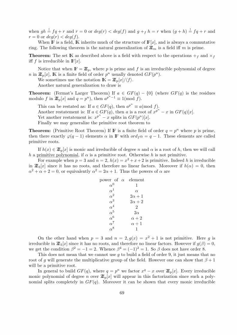
when gh =! fq + r and r = 0 or deg(r) < deg(f) and g +f h = r when (g + h) =! fq + r andr = 0 or deg(r) < deg(f).

When IF is a field, IK inherits much of the structure of IF[x], and is always a commutativering. The following theorem is the natural generalization of ZZm is a field iff m is prime.

Theorem: The set IK as described above is a field with respect to the operations +f and ×f

iff f is irreducible in IF[x].

Notice that when IF = ZZp, where p is prime and f is an irreducible polynomial of degreen in ZZp[x], IK is a finite field of order pn usually denoted GF (pn).

We sometimes use the notation IK = ZZp[x]/⟨f⟩.Another natural generalization to draw is

Theorem: (Fermat’s Larger Theorem) If a ∈ GF (q) − {0} (where GF (q) is the residuesmodulo f in ZZp[x] and q = pn), then ap

n−1 ≡ 1(mod f).

This can be restated as: If a ∈ GF (q), then apn ≡ a(mod f).

Another restatement is: If a ∈ GF (q), then a is a root of xpn − x in GF (q)[x].Yet another restatement is: xpn − x splits in GF (pn)[x].Finally we may generalize the primitive root theorem to

Theorem: (Primitive Root Theorem) If IF is a finite field of order q = pn where p is prime,then there exactly φ(q − 1) elements α in IF with ordfα = q − 1. These elements are calledprimitive roots.

If h(x) ∈ ZZp[x] is monic and irreducible of degree n and α is a root of h, then we will callh a primitive polynomial, if α is a primitive root. Otherwise h is not primitive.

For example when p = 3 and n = 2, h(x) = x2+x+2 is primitive. Indeed h is irreduciblein ZZ3[x] since it has no roots, and therefore no linear factors. Moreover if h(α) = 0, thenα2 + α+ 2 = 0, or equivalently α2 = 2α+ 1. Thus the powers of α are

power of α elementα0 1α1 αα2 2α+ 1α3 2α+ 2α4 2α5 2αα6 α+ 2α7 α+ 1α8 1

On the other hand when p = 3 and n = 2, g(x) = x2 + 1 is not primitive. Here g isirreducible in ZZ3[x] since it has no roots, and therefore no linear factors. However if g(β) = 0,we get the condition β2 = −1 = 2. Whence β4 = (−1)2 = 1. So β does not have order 8.

This does not mean that we cannot use g to build a field of order 9, it just means that noroot of g will generate the multiplicative group of the field. However one can show that β + 1will be a primitive root.

In general to build GF (q), where q = pn we factor xq − x over ZZp[x]. Every irreduciblemonic polynomial of degree n over ZZp[x] will appear in this factorization since such a poly-nomial splits completely in GF (q). Moreover it can be shown that every monic irreducible

69

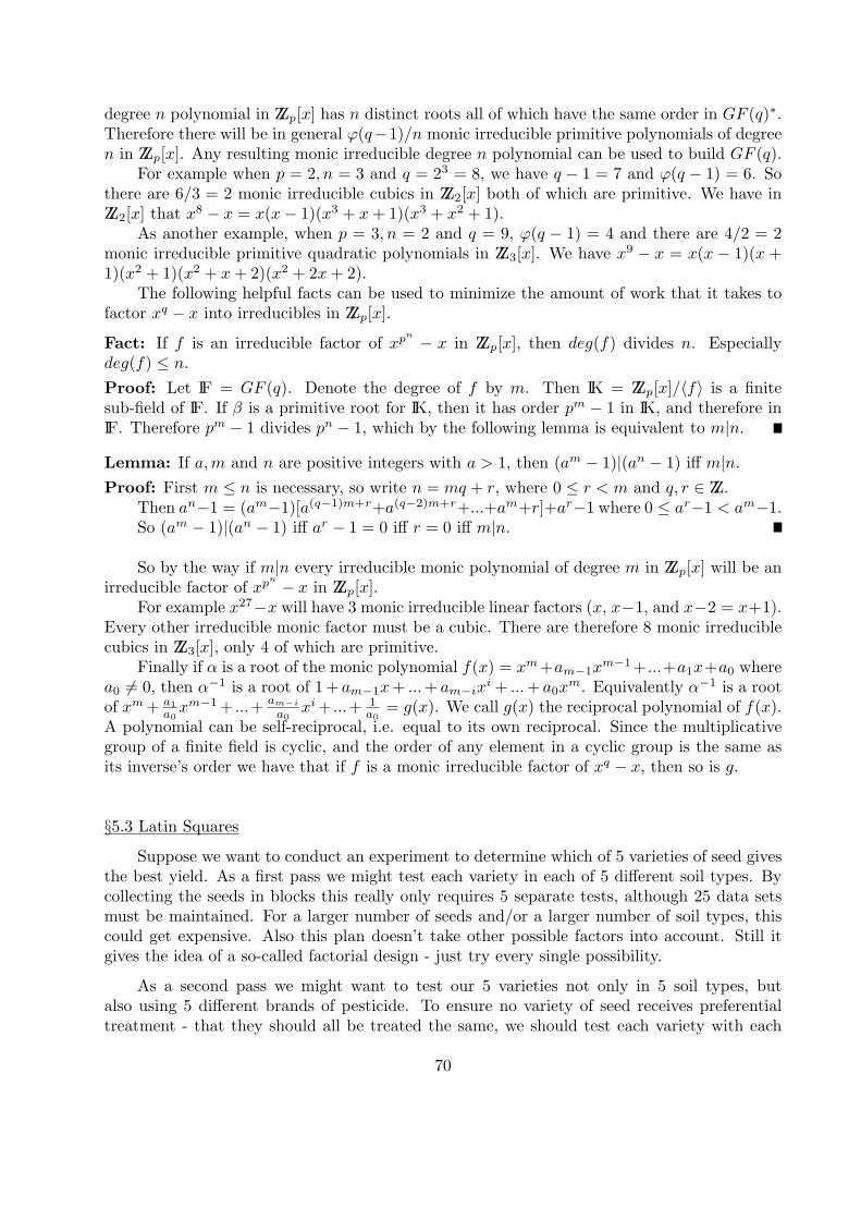
degree n polynomial in ZZp[x] has n distinct roots all of which have the same order in GF (q)∗.Therefore there will be in general φ(q−1)/n monic irreducible primitive polynomials of degreen in ZZp[x]. Any resulting monic irreducible degree n polynomial can be used to build GF (q).

For example when p = 2, n = 3 and q = 23 = 8, we have q − 1 = 7 and φ(q − 1) = 6. Sothere are 6/3 = 2 monic irreducible cubics in ZZ2[x] both of which are primitive. We have inZZ2[x] that x

8 − x = x(x− 1)(x3 + x+ 1)(x3 + x2 + 1).As another example, when p = 3, n = 2 and q = 9, φ(q − 1) = 4 and there are 4/2 = 2

monic irreducible primitive quadratic polynomials in ZZ3[x]. We have x9 − x = x(x − 1)(x +1)(x2 + 1)(x2 + x+ 2)(x2 + 2x+ 2).

The following helpful facts can be used to minimize the amount of work that it takes tofactor xq − x into irreducibles in ZZp[x].

Fact: If f is an irreducible factor of xpn − x in ZZp[x], then deg(f) divides n. Especiallydeg(f) ≤ n.

Proof: Let IF = GF (q). Denote the degree of f by m. Then IK = ZZp[x]/⟨f⟩ is a finitesub-field of IF. If β is a primitive root for IK, then it has order pm − 1 in IK, and therefore inIF. Therefore pm − 1 divides pn − 1, which by the following lemma is equivalent to m|n.

Lemma: If a,m and n are positive integers with a > 1, then (am − 1)|(an − 1) iff m|n.Proof: First m ≤ n is necessary, so write n = mq + r, where 0 ≤ r < m and q, r ∈ ZZ.

Then an−1 = (am−1)[a(q−1)m+r+a(q−2)m+r+...+am+r]+ar−1 where 0 ≤ ar−1 < am−1.So (am − 1)|(an − 1) iff ar − 1 = 0 iff r = 0 iff m|n.

So by the way if m|n every irreducible monic polynomial of degree m in ZZp[x] will be anirreducible factor of xpn − x in ZZp[x].

For example x27−x will have 3 monic irreducible linear factors (x, x−1, and x−2 = x+1).Every other irreducible monic factor must be a cubic. There are therefore 8 monic irreduciblecubics in ZZ3[x], only 4 of which are primitive.

Finally if α is a root of the monic polynomial f(x) = xm+am−1xm−1+ ...+a1x+a0 where

a0 = 0, then α−1 is a root of 1+ am−1x+ ...+ am−ixi + ...+ a0x

m. Equivalently α−1 is a rootof xm+ a1

a0xm−1+ ...+ am−i

a0xi+ ...+ 1

a0= g(x). We call g(x) the reciprocal polynomial of f(x).

A polynomial can be self-reciprocal, i.e. equal to its own reciprocal. Since the multiplicativegroup of a finite field is cyclic, and the order of any element in a cyclic group is the same asits inverse’s order we have that if f is a monic irreducible factor of xq − x, then so is g.

§5.3 Latin Squares

Suppose we want to conduct an experiment to determine which of 5 varieties of seed givesthe best yield. As a first pass we might test each variety in each of 5 different soil types. Bycollecting the seeds in blocks this really only requires 5 separate tests, although 25 data setsmust be maintained. For a larger number of seeds and/or a larger number of soil types, thiscould get expensive. Also this plan doesn’t take other possible factors into account. Still itgives the idea of a so-called factorial design - just try every single possibility.

As a second pass we might want to test our 5 varieties not only in 5 soil types, butalso using 5 different brands of pesticide. To ensure no variety of seed receives preferentialtreatment - that they should all be treated the same, we should test each variety with each

70

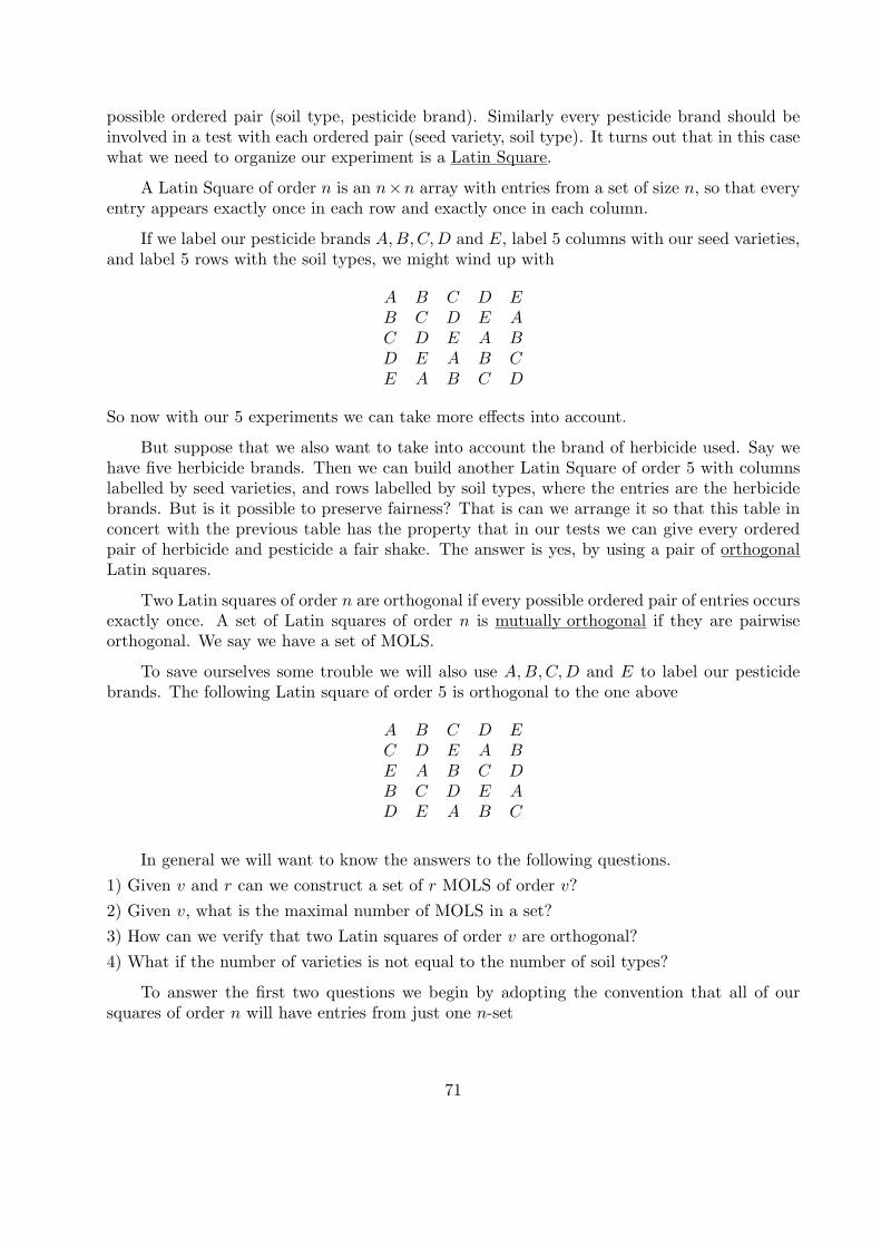
possible ordered pair (soil type, pesticide brand). Similarly every pesticide brand should beinvolved in a test with each ordered pair (seed variety, soil type). It turns out that in this casewhat we need to organize our experiment is a Latin Square.

A Latin Square of order n is an n×n array with entries from a set of size n, so that everyentry appears exactly once in each row and exactly once in each column.

If we label our pesticide brands A,B,C,D and E, label 5 columns with our seed varieties,and label 5 rows with the soil types, we might wind up with

A B C D EB C D E AC D E A BD E A B CE A B C D

So now with our 5 experiments we can take more effects into account.

But suppose that we also want to take into account the brand of herbicide used. Say wehave five herbicide brands. Then we can build another Latin Square of order 5 with columnslabelled by seed varieties, and rows labelled by soil types, where the entries are the herbicidebrands. But is it possible to preserve fairness? That is can we arrange it so that this table inconcert with the previous table has the property that in our tests we can give every orderedpair of herbicide and pesticide a fair shake. The answer is yes, by using a pair of orthogonalLatin squares.

Two Latin squares of order n are orthogonal if every possible ordered pair of entries occursexactly once. A set of Latin squares of order n is mutually orthogonal if they are pairwiseorthogonal. We say we have a set of MOLS.

To save ourselves some trouble we will also use A,B,C,D and E to label our pesticidebrands. The following Latin square of order 5 is orthogonal to the one above

A B C D EC D E A BE A B C DB C D E AD E A B C

In general we will want to know the answers to the following questions.

1) Given v and r can we construct a set of r MOLS of order v?

2) Given v, what is the maximal number of MOLS in a set?

3) How can we verify that two Latin squares of order v are orthogonal?

4) What if the number of varieties is not equal to the number of soil types?

To answer the first two questions we begin by adopting the convention that all of oursquares of order n will have entries from just one n-set

71

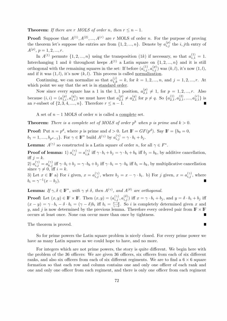
Theorem: If there are r MOLS of order n, then r ≤ n− 1.

Proof: Suppose that A(1), A(2), ..., A(r) are r MOLS of order n. For the purpose of proving

the theorem let’s suppose the entries are from {1, 2, ..., n}. Denote by a(p)i,j the i, jth entry of

A(p), p = 1, 2, ..., r.

In A(1) permute {1, 2, ..., n} using the transposition (1k) if necessary, so that a(1)1,1 = 1.

Interchanging 1 and k throughout keeps A(1) a Latin square on {1, 2, ..., n} and it is still

orthogonal with the remaining squares in the set: If before (a(1)i,j , a

(p)i,j ) was (k, l), it’s now (1, l),

and if it was (1, l), it’s now (k, l). This process is called normalization.

Continuing, we can normalize so that a(j)1,k = k, for k = 1, 2, ..., n, and j = 1, 2, ..., r. At

which point we say that the set is in standard order.

Now since every square has a 1 in the 1, 1 position, a(p)2,1 = 1, for p = 1, 2, ..., r. Also

because (i, i) = (a(p)1,i , a

(q)1,i ) we must have that a

(p)2,1 = a

(q)2,1 for p = q. So {a(1)2,1, a

(2)2,1, ...., a

(r)2,1} is

an r-subset of {2, 3, 4, ...., n}. Therefore r ≤ n− 1.

A set of n− 1 MOLS of order n is called a complete set.

Theorem: There is a complete set of MOLS of order pk when p is prime and k > 0.

Proof: Put n = pd, where p is prime and d > 0. Let IF = GF (pd). Say IF = {b0 = 0,

b1 = 1, ...., bpd−1}. For γ ∈ IF∗ build A(γ) by a(γ)i,j = γ · bi + bj .

Lemma: A(γ) so constructed is a Latin square of order n, for all γ ∈ F ∗.

Proof of lemma: 1) a(γ)i,j = a

(γ)i,k iff γ · bi + bj = γ · bi + bk iff bj = bk, by additive cancellation,

iff j = k.

2) a(γ)i,j = a

(γ)k,j iff γ · bi+ bj = γ · bk+ bj iff γ · bi = γ · bk iff bi = bk, by multiplicative cancellation

since γ = 0, iff i = k.

3) Let x ∈ IF a) For i given, x = a(γ)i,j , where bj = x − γ · bi. b) For j given, x = a

(γ)i,j , where

bi = γ−1(x− bj).

Lemma: If γ, δ ∈ IF∗, with γ = δ, then A(γ), and A(δ) are orthogonal.

Proof: Let (x, y) ∈ IF× IF. Then (x, y) = (a(γ)i,j , a

(δ)i,j ) iff x = γ · bi + bj , and y = δ · bi + bj iff

(x − y) = γ · bi − δ · bi = (γ − δ)bi iff bi =x−yγ−δ . So i is completely determined given x and

y, and j is now determined by the previous lemma. Therefore every ordered pair from IF× IFoccurs at least once. None can occur more than once by tightness.

The theorem is proved.

So for prime powers the Latin square problem is nicely closed. For every prime power wehave as many Latin squares as we could hope to have, and no more.

For integers which are not prime powers, the story is quite different. We begin here withthe problem of the 36 officers: We are given 36 officers, six officers from each of six differentranks, and also six officers from each of six different regiments. We are to find a 6× 6 squareformation so that each row and column contains one and only one officer of each rank andone and only one officer from each regiment, and there is only one officer from each regiment

72

of each rank. So the ranks give a Latin square, and the regiments, give an orthogonal Latinsquare.

In 1782, Leonhard Euler conjectured that this could not be done. In fact he conjecturedthat there was not a pair of MOLS for any positive whole number which was twice an oddnumber.

In 1900, a mathematician named John Tarry systematically checked all 9,408 pairs ofnormalized Latin squares of order 6 and showed that Euler was correct for this case. Nor-malization was an important part of Tarry’s proof, since there are 812,851,200 pairs of Latinsquares of order 6.

However in 1960, a trio of mathematicians proved that Euler was wrong in general.

Theorem: (Bose, Shrikhande, Parker) If n > 6 is twice an odd number, then there is a pairof MOLS of order n.

The proof of this theorem goes beyond the scope of our course, but we can discuss someof the tools that they had at hand, and why this was an important problem.

One of the most important construction techniques is due to MacNeish. In 1922 he usedwhat is commonly called the Kronecker product of matrices to build larger Latin squares fromsmaller ones. Given two square arrays, A of side m and B of side n, we can build a squarearray of side mn whose entries are ordered pairs (a, b). The first coordinate is the same forthe n × n block which is the intersection of the first n rows, and the first n columns. Thesecond coordinates in this block are simply the elements of B. In general the first coordinatefor the n×n block at the intersection of the (km+1)th through (km+n)th columns with the(jm+1)th through (jm+ n)th rows is the j, kth entry of A, while the second coordinates arethe entries of B. We will label the new square A⊗B.

Lemma: If A is a Latin square of order m, and B is a Latin square of order n, then A⊗ Bis a Latin square of order mn.

Proof: Exercise.

Theorem:(MacNeish) If there are r MOLS of order m and another r MOLS of order n, thenthere are r MOLS of order mn.

Proof: Let A(1), A(2), ..., A(r) be r MOLS of order m, and let B(1), B(2), ..., B(r) be r MOLSof order n. Put C(i) = A(i) ⊗ B(i), i = 1, 2, ..., r. Then the C(i)’s form a set of r MOLS oforder mn. The remainder of the proof is left as an exercise.

Corollary: Suppose that n > 1 has prime factorization pe11 pe22 ...pess , where all exponents arepositive whole numbers. Let r be the smallest of quantities peii − 1, i = 1, 2, ..., s. Then thereare at least r MOLS of order n.

Corollary: If n > 1 has prime factorization n = 2epe11 pe22 ...pess , where e = 1 and the pi’s areodd primes whose exponents are positive integers, then there is a pair of MOLS of order n.

So Bose, Shrikhande and Parker really had only to show existence of a pair of MOLS oforder 2p, for all odd primes p > 3. This noteworthy accomplishment touched off a flurry ofresearch in this area which lasted a good twenty years.

73

There are however many unanswered questions here. For example, for n = 10 are therethree MOLS of order 10? What is the largest value of r so that there is a set of r MOLS oforder 22?

Finally we mention the following, which may have been proven recently:

Conjecture: If there is a complete set of MOLS of order n, then n is a prime power.

The next section deals with our fourth question: What if the number of varieities is notequal to the number of soil types?

§5.4 Introduction to Balanced Incomplete Block Designs

In the preceding section we considered running experiments where we were given a certainnumber of varieties on which we wanted to run experiments under basic conditions. Almostnaively we had the number of varieties equal to the number of conditions, for each type ofcondition considered. If we consider the possibility of wanting to generate statistics for treadwear for automotive tires (vehicles with four wheels only) then we might have 8 differentbrands of tires and 10 different automobiles. Most importantly on any given car we couldrun experiments using at most four brands of tires. That is, when we separate our varietiesinto blocks we can no longer have all varieties per block. So we need to generalize the ideaof orthogonal Latin squares. The result of this abstraction will be objects called BalancedIncomplete Block Designs, or BIBDs for short.

A block design on a set V with |V | ≥ 2 consists of a collection B of non-empty subsets ofV called blocks. The elements of V are called varieties, or points.

A block design is balanced if all blocks have the same size k, every variety appears inexactly the same number of blocks r, and any two varieties are simultaneously in exactly λblocks.

A block design is incomplete in case k < v.

If V is a v-set of varieties and B a b-set of k-subsets of V , which are the blocks of a BIBDwhere every point is in r blocks, and every pair of points is in λ blocks we say that V and Bform a BIBD with parameters (b, v, r, k, λ). Equivalently a (b, v, r, k, λ)-BIBD means a BIBDwith parameters (b, v, r, k, λ).

Example: Let V = {0, 1, 2, 3, 4, 5, 6, 7, 8, 9, 10} and put B = {{1, 3, 4, 5, 9}, {2, 4, 5, 6, 10},{0, 3, 5, 6, 7}, {1, 4, 6, 7, 8}, {2, 5, 7, 8, 9}, {3, 6, 8, 9, 10}, {0, 4, 7, 9, 10}, {0, 1, 5, 8, 10},{0, 1, 2, 6, 9}, {1, 2, 3, 6, 10}, {0, 2, 3, 4, 8}}. Then V and B form an (11, 11, 5, 5, 2)-BIBD.

This example helps raise a number of pertinent questions

1) How do we know that this example really works, i.e. how can we verify that all pertinentconditions are actually satisfied?

2) What are necessary conditions, if any, which must be satisfied for a BIBD to exist?

3) What are sufficient conditions?

4) When a BIBD exists, is it essentially unique?, If so, why?, If not unique, how many essentiallydifferent configurations are there?

74

The remainder of this section will deal the second of these questions. Subsequent sectionswill address the remaining questions.

Lemma: In a BIBD with parameters (b, v, r, k, λ) we have bk = vr.

Proof: Count occurences of varieties in blocks two ways. On the one hand there are b blockseach consisting of k varieties. On the other hand there are v varieties each occuring in exactlyr blocks.

Lemma: In a BIBD with parameters (b, v, r, k, λ) we have λ(v − 1) = r(k − 1).

Proof: For a particular variety count pairs of varieties it occurs in blocks with two ways. Onthe one hand, there are v−1 other varieties that it must appear with in exactly λ blocks each.On the other hand this variety appears in exactly r blocks and in each block there are k − 1other varieties.

Example: The parameter set (12, 9, 4, 3, 2) satisfies the first lemma since 12 · 3 = 9 · 4, but itfails to satisfy the second condition 2 ·8 = 4 ·2. Therefore there can be no (12, 9, 4, 3, 2)-BIBD.

Example: The parameter set (43, 43, 7, 7, 1) satisfies both lemmata. However, as we’ll see,there is also no (43, 43, 7, 7, 1)-design. So we stress that the conditions from the lemmata arenecessary, but not sufficient.

It is useful when investigating BIBDs to represent them via incidence matrices similar towhat we did for graphs. An incidence matrix for a (b, v, r, k, λ)-BIBD is a v × b 0− 1 matrixwhose rows are labelled by the varieties, columns by blocks, and where the i, j entry is 1 incase the ith variety is in the jth block, and 0 if not.

Example: An incidence matrix for our example of an (11, 11, 5, 5, 2)-BIBD where the rows arelabelled in order 0, 1, 2, 3, 4, 5, 6, 7, 8, 9, 10 and the blocks are in reverse order except for thefirst one

0 1 0 1 1 1 0 0 0 1 01 0 1 1 1 0 0 0 1 0 00 1 1 1 0 0 0 1 0 0 11 1 1 0 0 0 1 0 0 1 01 1 0 0 0 1 0 0 1 0 11 0 0 0 1 0 0 1 0 1 10 0 0 1 0 0 1 0 1 1 10 0 1 0 0 1 0 1 1 1 00 1 0 0 1 0 1 1 1 0 01 0 0 1 0 1 1 1 0 0 00 0 1 0 1 1 1 0 0 0 1

We henceforth assume that the reader is familiar with the basics of matrix multiplication

and determinants.

An incidence matrix for a BIBD with parameters (b, v, r, k, λ) must have all column sumsequal to k, all row sums equal to r, and for i = j, the dot product of the ith row with the jthrow counts the number of columns in which both rows have a 1, which must equal λ. If wedenote the identity matrix of side n by In and the all 1’s matrix of size m by Jm we have

75

Lemma: An incidence matrix A for a (b, v, r, k, λ)-BIBD must satisfy the matrix equationAAT = (r − λ)Iv + λJv.

Proof: The i, j entry of AAT is the dot product of the ith row of A with the jth column ofAT , which is the dot product of the ith row of A and the jth row of A. This value is λ wheni = j and r when i = j.

Lemma: If A is an incidence matrix for a BIBD with parameters (b, v, r, k, λ), thendet(AAT ) = [r + (v − 1)λ](r − λ)v−1.

Proof:

det(AAT ) = det

r λ λ ... λλ r λ ... λ...

. . .. . .

. . ....

λ ... λ r λλ ... λ λ r

Adding the last v − 1 rows to the first row does not change the value of the determinant so

det(AAT ) = det

r + λ(v − 1) r + λ(v − 1) r + λ(v − 1) ... r + λ(v − 1)

λ r λ ... λ...

. . .. . .

. . ....

λ ... λ r λλ ... λ λ r

Next we factor r + λ(v − 1) out of the first row. So

det(AAT ) = [r + λ(v − 1)]det

1 1 1 ... 1λ r λ ... λ...

. . .. . .

. . ....

λ ... λ r λλ ... λ λ r

Subtract λ times the first row from each of the last v − 1 rows to get

det(AAT ) = [r + λ(v − 1)]det

1 1 1 ... 10 r − λ 0 ... 0...

. . .. . .

. . ....

0 ... 0 r − λ 00 ... 0 0 r − λ

From which the result follows.

A first application for the previous theorem follows from the fact that for an incompletedesign we have k < v. The constraint λ(v − 1) = r(k − 1) then implies that λ < r. So theprevious theorem shows that det(AAT ) > 0. Which led R.A. Fisher to the following theorem.

Theorem: (Fisher’s Inequality) For a BIBD with parameters (b, v, r, k, λ), v ≤ b.

76

Proof: If v > b we can pad an incidence matrix A for the design by adding v − b columnsof zeroes resulting in a matrix B with BBT = AAT . But since B has a column of zeroesdet(B) = det(BT ) = 0. So 0 = det(B)det(BT ) = det(BBT ) > 0, a contradiction.

When a BIBD with parameters (b, v, r, k, λ) has v = b, then the equation bk = vr impliesthat k = r too. We call a BIBD with parameters (v, v, k, k, λ) a (v, k, λ)-symmetric design, ora symmetric design with parameters (v, k, λ). The integer n = k − λ is called the order of thedesign. A second application of the determinant theorem explicitly for symmetric designs isdue to Schutzenberger.

Theorem: (Schutzenberger) For a symmetric design with parameters (v, k, λ), if v is even,then n = k − λ is a square.

Proof: Let D be a (v, k, λ)-symmetric design and A an incidence matrix for D. Since r = kthe equation λ(v−1) = r(k−1) now reads λ(v−1) = k(k−1). So r+λ(v−1) = k+k(k−1) =k + k2 − k = k2. Thus

[det(A)]2 = det(A)det(AT ) = det(AAT ) = [r + λ(v − 1)](k − λ)v−1 = k2nv−1.

Since the left hand side is a square, the right hand side must be too. But the exponent on nis odd, which means that n must be a square.

Example: Consider a putative symmetric design with parameters (22, 7, 2). These parameterssatisfy both earlier lemmata. However v = 22 is even, and n = 5 is not a square. Thereforeno such design can exist.

§5.5 Sufficient Conditions for, and Constructions of BIBDs

A design with block size k = 3 is called a triple system. If in addition λ = 1, we havewhat we call a Steiner Triple System, or STS. Notice that for an STS, given v, we can find band r from the lemmata of the previous section. So the parameter set of an STS is completelydetermined as soon as we know v. We call a Steiner Triple System on v varieties a STS(v).

Ten years before Steiner considered these objects the Rev. T.P. Kirkman considered themand proved:

Theorem: There exist an STS(v) with1) v = 6n+ 1, b = nv, and r = 3n for all n ∈ ZZ+

2) v = 6n+ 3, b = (3n+ 1)(2n+ 1), and r = 3n+ 1, for all n ∈ ZZ+

This theorem is a corollary of the following theorem, and known constructions of smallerSTS’s.

Theorem: If D1 is an STS(v1) and D2 is an STS(v2), then there exists an STS(v1v2).

Proof: Let the varieties of D1 be a1, a2, ...av1 , and the varieties of D2 be b1, b2, ..., bv2 . Letcij 1 ≤ i ≤ v1, 1 ≤ j ≤ v2 be a set of v1 · v2 symbols. Define the blocks of an STS(v1v2) by{cir, cjs, ckt} is a block iff one of the following conditions holds

1) r = s = t and {ai, aj , ak} is a block of D1

77

2) i = j = k and {br, bs, bt} is a block of D2

3) {ai, aj , ak} is a block of D1, and {br, bs, bt} is a block of D2.

Now check that all properties are satisfied.

To find small STS’s, and other designs there are a number of construction techniques. Thefirst way is to find what is called a difference set. A difference set D with parameters (v, k, λ),aka a (v, k, λ)-difference set, is a k-subset of a group G of order v, written multiplicatively, sothat every g ∈ G− {1} is writable as d−1

2 d1 for exactly λ pairs d1, d2 ∈ D, with d1 = d2.

Example: Let G be the integers modulo 13 written additively. D = {0, 1, 3, 9} is a (13, 4, 1)-difference set in G as can be seen by the following table of differences.

− 0 1 3 90 0 12 10 41 1 0 11 53 3 2 0 79 9 8 6 0

For a difference D in a group G the set Dg = {dg|d ∈ d} is called a translate of the differenceset. From the previous example D + 5 = {5, 6, 8, 1}.

Theorem: If D is a (v, k, λ)-difference set in a group G, then the set of translates {Dg|g ∈ G}form the blocks of a symmetric (v, k, λ)-design where G is the set of varieties.

Proof: First notice that the number of translates is v. Also each translate has cardinality kby the group cancellation law. A group element g is in the translate Dgi iff there is di ∈ Dwith g = digi. There are k chioces for di, there are therefore k choices for gi = d−1

i g. So wehave v varieties, v blocks, each block of cardinality k, and each variety in k blocks. It remainsto show that any pair of varieties is in exactly λ blocks together. So let g1 = g2 be two groupelements. Put x = g2g

−11 . x appears exactly λ times as d−1

2 d1 for d1, d2 ∈ D with d1 = d2.There are therefore exactly λ solutions in d1 and d2 to the equation d−1

2 d1 = g2g−11 = x. That

is, exactly λ times we have d1g1 = d2g2, with d1, d2 ∈ D. Thus |Dg1 ∩Dg2| = λ.

Example: Starting with the block D+0 = {0, 1, 3, 9}, we build a (13, 4, 1)-design with varietiesfrom ZZ13 = {0, 1, 2, 3, 4, 5, 6, 7, 8, 9, 10, 11, 12} and remaining blocks D + 1 = {1, 2, 4, 10},D + 2 = {2, 3, 5, 11}, D + 3 = {3, 4, 6, 12}, D + 4 = {0, 4, 5, 7}, D + 5 = {1, 5, 6, 8},D + 6 = {2, 6, 7, 9}, D + 7 = {3, 7, 8, 10}, D + 8 = {4, 8, 9, 11}, D + 9 = {5, 9, 10, 12},D + 10 = {0, 6, 10, 11}, D + 11 = {1, 7, 11, 12}, and D + 12 = {0, 2, 8, 12}.

For a (v, k, λ)-difference set, the number n = k−λ is called the order. It is often the casethat the difference set is left invariant by a multiplier. In fact frequently a prime dividing nwill be a multiplier.

Example: From our (13, 4, 1)-difference set in ZZ13 we have n = 3 which is prime. We candecompose ZZ13 into orbits under multiplication by 3. For g ∈ ZZ13 its orbit will be [g] ={3kg|k ∈ ZZ}. So we have [0] = {0}, [1] = {1, 3, 9}, [2] = {2, 6, 5}, [4] = {4, 12, 10}, [7] ={7, 8, 11}. Notice that the difference set is the union of orbits. Therefore 3 is a multiplier forthis difference set.

78

The term difference set comes from the fact that the first examples of this kind of behaviorwere discovered by Gauss. In his famous book Disquisitiones Arithmeticae Gauss essentiallyproves the following theorem which we present without proof.

Theorem: Let p be a prime congruent to 3 modulo 4. The set of quadratic residues modulop, which are those numbers x ∈ ZZ∗

p so that there is a y ∈ ZZ∗p with x = y2, form a

(p, (p− 1)/2, (p− 3)/4)-difference set in ZZp.

There are many other results on difference sets. It is also true that this method generalizesto what is called the method of mixed differences. This more general method is often usedto generate designs which are not symmetric designs by starting with a collection of starterblocks. For the method above, we have only one starter block - namely the difference set.

We close this section with a short list of methods which allow us to build new designsfrom a given design.

Replication: By simply repeating every block of a (b, v, r, k, λ)-design l times we can build a(bl, v, rl, k, λl)-design.

Complementation: For a (b, v, r, k, λ)-design on V with blocks {a1, ..., ab} the complementarydesign has blocks {V − a1, ..., V − ab} and parameters (b, v, b− r, v − k, b− 2r + λ). So up tocomplementation we can take 2k < v.

Set Difference: Starting with a symmetric (v, k, λ)-design with blocks a1, ..., av select someblock ai to delete, and remove all points on that block from the remaining blocks. So we geta (v − 1, v − k, k, k − λ, λ)-design on V − ai with blocks aj − ai, for i = j and 1 ≤ j ≤ v.

Restriction: Again start with a symmetrtic (v, k, λ)-design with blocks a1, ..., av. Now selecta block ai and for j = i form new blocks aj ∩ ai. This gives a (v − 1, k, k − 1, λ, λ− 1)-designas long as λ > 1.

§5.6 Finite Plane Geometries

The last major source of designs we wish to discuss are those coming from finite geometries.This is an incredibly rich area for research questions, especially if one does not assume that afinite field is used to coordinatize the space. We will stick to the relatively safe realm wherewe assume that we have a finite field IF of order q = pn for some prime integer p. We will alsodeal mainly with low dimensional geometries, namely planes.

Similar to continuous mathematics we can consider IF2 as a Cartesian product coordina-tizing a plane. It’s just that in this case because IF is finite, there will be only finitely manypoints in our plane, which we will denote EG(2, q). EG stands for Euclidean Geometry, and2 corresponds to the dimension.

In fact we clearly have exactly q2 points in our plane, since any point can be coordinatizedby an ordered pair (x, y), where x, y ∈ IF.

The other natural objects from Euclidean geometry to consider are lines, which over afield satisfy equations of the form Ax+By = D, where not both A and B are zero. In fact ifB = 0 we can re-write our line in point-intercept form y = mx+ b, where m is the slope, and bis the y-intercept. If B = 0, then A = 0 and we get the so-called vertical lines with equationsx = c. There are q2 lines of the first form since m, b ∈ IF. And there are q lines of the formx = c since c ∈ IF.

79

By the properties of a field each line will contain exactly q points. Also every point willbe on exactly q + 1 lines – one for each slope in IF, and one with infinite slope (vertical).

Finally, any two points determine a unique line. So the points and lines of EG(2, q) forma (q2 + q, q2, q + 1, q, 1)-design.

This design is slightly different from previous examples in that it is resolvable. This justmeans that blocks come in “parallel” classes - blocks from a parallel class partition the varietyset.

If we extend every line of slope m to∞, we get the effect of looking down a pair of parallelrailroad tracks - which we perceive as intersecting eventually. Let the common point at infinitywhich is the intersection of all lines of slope m be labelled (m). Include the point (∞) as theintersection of all of the vertical lines. Finally connect all of these points at infinity with a lineat infinity. The result will be a new structure with q + 1 new points and 1 new line. We callthis PG(2, q). PG stands for projective geometry.

The points and lines of PG(2, q) form a symmetric (q2 + q + 1, q + 1, 1)-design. It can beshown that the existence of such a design is equivalent to a complete set of MOLS of order q.It can also be shown that the result of performing the set difference construction starting witha projective plane of order q and using the line at infinity gives an affine plane of order q. Infact any line (not just the one at inifinity) can be used.

Another way to construct PG(2, q) is to define its points to be the one-dimensional sub-spaces of IF3, and its lines to be the two-dimensional subspaces. A point is on a line, if thecorresponding one-dimensional subspace is included in the two-dimensional subspace.

Now any “point” is completely determined by a direction vector v = ⟨0, 0, 0⟩. We assignthe components of v as the homogeneous coordinates of the point, with the convention thattwo sets of homogeneous coordinates determine the same point iff they are in a common ratio,that is [a : b : c] = [d : e : f ] iff there is α ∈ IF∗ with ⟨a, b, c⟩ = α⟨d, e, f⟩.

Given a point with homogeneous coordinates [a : b : c] and c = 0, the point also hascoordinates [a/c : b/c : 1] := [x : y : 1]. We call such a point a “finite” point and let itcorrespond to (x, y) ∈ IF2. If c = 0, then say x = 0, which means [x : y : 0] = [1 : y/x : 0] :=[1 : m : 0]. So the points at infinity labelling non-infinite slopes of lines are (m) = [1 : m : 0].Finally, if both a = c = 0, then b = 0 and [0 : b : 0] = [0 : 1 : 0] = (∞).

We can also use homogeneous coordinates for the lines, but commonly represent themas column vectors. Any line is really a plane through (0, 0, 0) in IF3, and so is completelydetermined by its normal vector. The point [x : y : z] lies on the line [A : B : C]T in caseAx+By + Cz = 0.

A line [A : B : C]T with B = 0 is the same as the line [−m : 1 : −b]T , where m = −A/Band b = −C/B. These have equation y = mx + b in the finite part of the plane. A line withB = 0 but A = 0 is [1 : 0 : −c]T , where −c = −C/A. These have equation x = c in the finitepart of the plane. Finally, the line at infinity l∞ has coordinates [0, 0, 1]T .

80

Chapter 5 Exercises1. Show that x2 +1 is irreducible mod 3. Show that if α2 +1 = 0 (mod 3), then α has order4 in GF(9). Hence x2 + 1 is not a primitive polynomial mod 3.

2. Show that x2 + 2x + 2 is irreducible mod 3. Show that if α2 + 2α + 2 = 0 mod 3, then αhas order 8 in GF(9). Hence x2 + 2x+ 2 is a primitive polynomial modulo 3.

3. Find the multiplicative inverse of 8 in a) GF(11), b) GF(13), c) GF(17).

4. In GF(7) solve the equationsx+ 2y + 3z = 2

2x+ 4y + 5z = 6

3x+ y + 6z = 4

5. Show that 5 is a primitive root modulo 23.

6. Find all monic irreducible quadratic polynomials mod 5.

7. Let p = 2 and n = 4a) How many monic irreducible quartics are there in ZZp[x]?b) How many primitive monic irreducible quartics are there in ZZp[x]?c) How many self-reciprocal monic irreducible quartics are there in ZZp[x]?

Use a-c to factor xp4 − x into monic irreducible factors in ZZp[x].

8. Show that q(x) = x2 + 1 is reducible mod 5. Repeat mod 7. Is q(x) primitive mod 7?

9. Show that the probability that a monic irreducible cubic is primitive in ZZ5[x] is12 .

10. Show that x4 + x+ 1 is primitive in ZZ2[x].

11. Find a primitive root modulo 31.

12. For each value of n determine how many mutually orthogonal Latin squares can beconstructed using MacNeish’s Theorem.

a) n = 12 b) n = 13 c) n = 21 d) n = 25

e) n = 35 f) n = 36 g) n = 39 h) n = 75

i) n = 140 j) n = 185 k) n = 369 l) n = 539

13. Describe how you would construct 10 MOLS of order 275.

14. Construct a complete set of MOLS of order 5.

15. Repeat exercise 3, with squares of order 7.

16. Repeat exercise 3, with squares of order 8.

17. For each of the following block designs, determine if the design is a BIBD and if so computeits parameters b, v, r, k, and λ.

a) Varieties: {1, 2, 3}Blocks: {1, 2}, {1, 3}, {2, 3}, {1, 2, 3}

b) Varieties: {1, 2, 3, 4, 5}Blocks: {1, 2, 3}, {2, 3, 4}, {3, 4, 5}, {1, 4, 5}, {1, 2, 5}

81

c) Varieties: {1, 2, 3, 4, 5}Blocks: {1, 2, 3, 4}, {1, 3, 4, 5}, {1, 2, 4, 5}, {1, 2, 3, 5}, {2, 3, 4, 5}

d) Varieties: {1, 2, 3, 4, 5, 6, 7, 8, 9}Blocks: {1, 2, 3}, {4, 5, 6}, {7, 8, 9}, {1, 4, 7}, {2, 5, 8}, {3, 6, 9}

{1, 5, 9}, {2, 6, 7}, {3, 4, 8}, {1, 6, 8}, {2, 4, 9}, {3, 5, 7}

18. Find an incidence matrix for each design from exercise 17.

19. If a BIBD has parameters v = 15, k = 10, and λ = 9, find b and r.

20. If a BIBD has parameters v = 47 = b, and r = 23, find k and λ.

21. If a BIBD has parameters b = 14, k = 3, and λ = 2, find v and r.

22. Show that there is no (7, 5, 4, 3, 2)−BIBD.

23. Show that there is no (22, 22, 7, 7, 1)-BIBD.

24. For a Steiner triple system with v = 9, find b and r.

25. The following nine blocks form part of a Steiner triple system on {a, b, c, d, e, f, g, h, i}:{a, b, c}, {d, e, f}, {g, h, i}, {a, d, g}, {c, e, h}, {b, f, i}, {a, e, i}, {c, f, g}, {b, d, h}Add the remaining blocks to complete the design.

26. Four of the blocks of a symmetric (7,3,1)-design are {1, 2, 3}, {2, 4, 6}, {3, 4, 5}, {3, 6, 7}.Find the remaining blocks.

27. Find a (11, 5, 2)-difference set in ZZ11. Display the table of differences.

28. Find a (13, 4, 1)-difference set in ZZ13. Display the table of differences.

29. Find a (21, 5, 1)-difference set in ZZ21. Display the table of differences.

30. Find a (16, 6, 2)-difference set in ZZ42. Display the table of differences.

31. Use your answer from exercise 30 to construct a 16× 16 matrix, H, whose entries are all±1, and for which H = HT , and H2 = 16I16.

32. If α is the primitive root of GF (9) = ZZ3/ < x2 + 2x + 2 >, find all points on the lineαx+ α3y = α7 in EG(2, 9).

33. Find the point of intersection of the lines 2x+ y = 5 and 3x+ 4y = 6 in EG(2, 7).

34. For the geometry EG(2, 4) find equations for every line and determine which points areincident with each line.

82

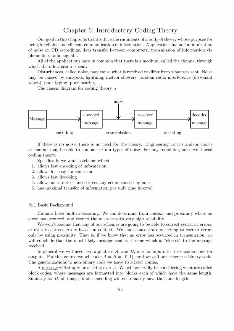
Chapter 6: Introductory Coding Theory

Our goal in this chapter is to introduce the rudiments of a body of theory whose purpose forbeing is reliable and efficient communication of information. Applications include minimizationof noise on CD recordings, data transfer between computers, transmission of information viaphone line, radio signal...

All of the applications have in common that there is a medium, called the channel throughwhich the information is sent.

Disturbances, called noise, may cause what is received to differ from what was sent. Noisemay be caused by sunspots, lightning, meteor showers, random radio interference (dissonantwaves), poor typing, poor hearing,....

The classic diagram for coding theory is

Message

encoding

encoded

message

noise

transmission

received

message

decoding

decoded

message

..........................................................................................................................................................................................................

..........................................................................................................................................................................................................

.........................................................................................................................

.........................................................................................................................

.........................................................................................................................

.........................................................................................................................

.....................................................................................................

.....................................................................................................

.....................................................................................................

.....................................................................................................

.....................................................................................................

.....................................................................................................

.....................................................................................................

.....................................................................................................

............................................................................................................................................................................................... ..................................................................................................................................................................................... ...............................................................................................................................................................................................

..................................................................................................................................................................

............................................................................

If there is no noise, there is no need for the theory. Engineering tactics and/or choiceof channel may be able to combat certain types of noise. For any remaining noise we’ll needcoding theory.

Specifically we want a scheme which1. allows fast encoding of information2. allows for easy transmission3. allows fast decoding4. allows us to detect and correct any errors caused by noise5. has maximal transfer of information per unit time interval

§6.1 Basic Background

Humans have built-in decoding. We can determine from context and proximity where anerror has occurred, and correct the mistake with very high reliability.

We won’t assume that any of our schemes are going to be able to correct syntactic errors,or even to correct errors based on context. We shall concentrate on trying to correct errorsonly by using proximity. That is, if we know that an error has occurred in transmission, wewill conclude that the most likely message sent is the one which is “closest” to the messagereceived.

In general we will need two alphabets A, and B, one for inputs to the encoder, one foroutputs. For this course we will take A = B = {0, 1}, and we call our scheme a binary code.The generalizations to non-binary code we leave to a later course.

A message will simply be a string over A. We will generally be considering what are calledblock codes, where messages are formatted into blocks each of which have the same length.Similarly for B, all images under encoding will customarily have the same length.

83

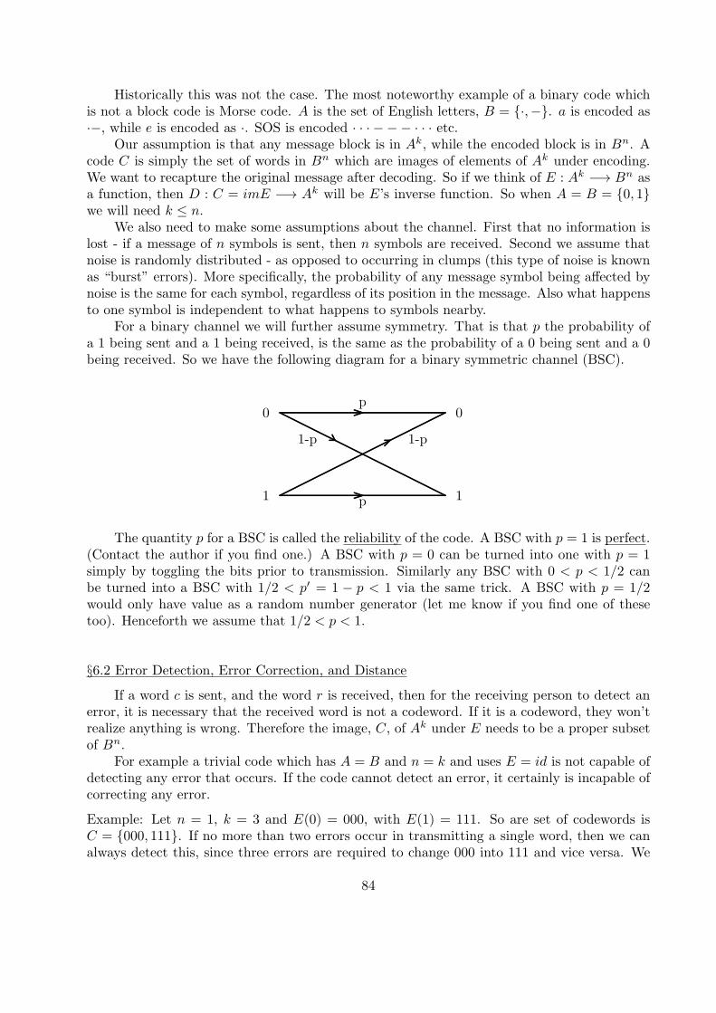
Historically this was not the case. The most noteworthy example of a binary code whichis not a block code is Morse code. A is the set of English letters, B = {·,−}. a is encoded as·−, while e is encoded as ·. SOS is encoded · · · − − − · · · etc.

Our assumption is that any message block is in Ak, while the encoded block is in Bn. Acode C is simply the set of words in Bn which are images of elements of Ak under encoding.We want to recapture the original message after decoding. So if we think of E : Ak −→ Bn asa function, then D : C = imE −→ Ak will be E’s inverse function. So when A = B = {0, 1}we will need k ≤ n.

We also need to make some assumptions about the channel. First that no information islost - if a message of n symbols is sent, then n symbols are received. Second we assume thatnoise is randomly distributed - as opposed to occurring in clumps (this type of noise is knownas “burst” errors). More specifically, the probability of any message symbol being affected bynoise is the same for each symbol, regardless of its position in the message. Also what happensto one symbol is independent to what happens to symbols nearby.

For a binary channel we will further assume symmetry. That is that p the probability ofa 1 being sent and a 1 being received, is the same as the probability of a 0 being sent and a 0being received. So we have the following diagram for a binary symmetric channel (BSC).

0 0

1 1

p

p

1-p 1-p

..................................................................................................................................................................................................................................................................................................................................................................................................................................................................................................................................................................................................................................................................................................................................................................................................................................................................................................................................................................................................................................

........................................................

........................................................

........................................................

........................................................

........................................................

................................

................................

........... ....................... ...............

The quantity p for a BSC is called the reliability of the code. A BSC with p = 1 is perfect.(Contact the author if you find one.) A BSC with p = 0 can be turned into one with p = 1simply by toggling the bits prior to transmission. Similarly any BSC with 0 < p < 1/2 canbe turned into a BSC with 1/2 < p′ = 1 − p < 1 via the same trick. A BSC with p = 1/2would only have value as a random number generator (let me know if you find one of thesetoo). Henceforth we assume that 1/2 < p < 1.

§6.2 Error Detection, Error Correction, and Distance

If a word c is sent, and the word r is received, then for the receiving person to detect anerror, it is necessary that the received word is not a codeword. If it is a codeword, they won’trealize anything is wrong. Therefore the image, C, of Ak under E needs to be a proper subsetof Bn.

For example a trivial code which has A = B and n = k and uses E = id is not capable ofdetecting any error that occurs. If the code cannot detect an error, it certainly is incapable ofcorrecting any error.

Example: Let n = 1, k = 3 and E(0) = 000, with E(1) = 111. So are set of codewords isC = {000, 111}. If no more than two errors occur in transmitting a single word, then we canalways detect this, since three errors are required to change 000 into 111 and vice versa. We

84

therefore call C a 2-error detecting code. C is also a 1-error correcting code, since if we supposethat no more than one error occurs, any received word is either a codeword, or is uniquely thecause of a single error affecting one of our two codewords. This ability comes at the price thatour rate of information is essentially 1/3, 1 bit of information being conveyed for every 3 bitssent.

The essential property of the code in the last example which allows it to detect and correcterrors is distance. Given two vectors of the same length, their Hamming distance is the numberof positions where they differ. The distance of a code C is the minimum distance among alldistinct pairs of codewords. Notice that for binary codes the Hamming distance d(x, y) is thenumber of 1’s in the string x+ y where addition is componentwise mod 2. The number of 1sin a binary string, z, is called its weight and is denoted by wt(z). So d(x, y) = wt(x+ y) for abinary code.

If we now further assume that the probability of fewer errors occuring is higher thanthe probability of a large number of errors occuring we arrive at the principle of MaximumLikelihood Decoding: Suppose that a word r is received and it is detected that r is not acodeword. In case there is a unique codeword c that is closest to r (the Hamming distancefrom r to c is minimum), decode r as c.

In our preceeding example the code C clearly has distance 3 since 000 and 111 differ inall three positions. We write d(000, 111) = 3. From our previous discussion we get.

Theorem: For a binary code C, let δ = minv =w∈Cd(v, w). Then C can detect up to δ − 1errors, but there is a way that δ errors can occur which cannot be detected.

More importantly

Theorem: If C is a code with minimum distance δ and t = ⌈(δ/2) − 1⌉, then C can correctup to t errors by using Maximum Likelihood Decoding, but there will be a way for t+ 1 errorsto occur and correction is not possible.

Notice that the probability of errors occuring comes into play in our assumptions. Fromthe binomial theorem we have the following corollary.

Theorem: In a BSC with reliability p, the probability that exactly r errors will occur in

transmitting a bit string of length n is given by

(n

r

)(1− p)rpn−r.

Example: When n = 7 and p = 0.99 the probability that exactly one error occurs is(7

1

)(0.01)1(0.99)6 ≈ 0.0659036. The probability that no error occurs is(

7

0

)(0.01)0(0.99)7 ≈ 0.9320653. The probability that exactly two errors occur is(

7

2

)(0.01)2(0.99)5 ≈ 0.0019971. So the probability that more than two errors occur is about

0.00003397.

Example: If n = 11 and p = 1 − 10−8, and the rate of transmission is 107 digits/second theprobability that a word of length n = 11 is transmitted incorrectly is about 11p10(1 − p).

Since 107/11 words are transmitted each second, we can expect 11108 ·

107

11 ≈ 0.1 words/secondto be transmitted incorrectly, which translates into 8640 words transmitted incorrectly each

85

day. If we add a single parity check digit at the end of each word, to make the numberof ones in the word even, then the probability of at least 2 errors occuring per codeword is1 − p12 − 12p11(1 − p) ≈ 66/1016. Now we find that we can expect to wait about 2000 daysbefore an undetectable set of errors occurs.

R.W. Hamming was one of the original contributors to coding theory. Among other thingshe is credited with the following bound on the size of a code given its minimum distance.

Theorem: (Hamming Bound) If C is a binary code of length n and minimum distance δ, then

|C| ≤ 2n(n0

)+(n1

)+ ...+

(nt

) , where t = ⌈(δ/2)− 1⌉.

Proof: Let s ∈ C. Denote by Br(s) those bit strings of length n which have Hamming distance

exactly r from s. Note that |Br(s)| =(n

r

)since we simply choose the r positions from s to

change.Now denote by B′

m(s) the set of bit strings of length n which are at distance at most m

from s (inclusive). Now |B′m(s)| =

(n

0

)+

(n

1

)+ ...+

(n

m

).

If t = ⌈(δ/2) − 1⌉, then B′t(s1) ∩ B′

t(s2) = ∅ for all s1, s2 ∈ C. Thus any bit string oflength n is in at most one set B′

t(s).

Therefore |C||B′t(s)| =

∑s∈C

|B′t(s)| ≤ | ∪s∈C B′

t(s)| ≤ 2n.

§6.3 Linear Codes

Almost all coding schemes in use are what are known as linear codes. To say that abinary code C is linear, means that if x, y ∈ C, then x + y ∈ C. So a linear binary codeis a k-dimensional subspace of ZZn

2 . Thus there is a set of codewords {b1, ..., bk} (a basis),so that every codeword c ∈ C is (uniquely) a linear combination of the basis vectors, i.e.c = α1b1 + α2b2 + ...+ αkbk.

Notice, that every binary code contains the all 0s word since if c ∈ C, c+ c = 0 ∈ C. Alsonotice that the minimum distance in a linear code coincides with the minimum weight takenover all non-zero code words. This is true because d(x, y) = wt(x + y), and for a linear codex+ y is always a code word when x and y are.

The k×n matrix M whose rows are b1, ..., bk is a generating matrix for C. In general anymatrix whose rows form a basis for C is a generating matrix for C. Most linear codes have agenerating matrix which takes standard form. The generating matrix for a code in standardform consists of a k × k identity matrix appended with a k × (n− k) matrix G.

For a binary linear code C, encoding is accomplished by vector-matrix multiplication.If v ∈ {0, 1}k is a message word, E(v) = vM , where M is a generating matrix for C, andall arithmetic is performed mod 2. When M is in standard form E(v) = (v|vG), so theinformation bits of a word are preserved in the first k bits of the code word. Thus if no errorsoccur decoding amounts to stripping off the first k bits of every codeword received. Life ismore interesting when errors do occur.

To detect whether errors have occurred we use what’s called a parity check matrix. Aparity check matrix for a binary linear code C of dimension k and length n, is an (n− k)× nmatrix H, so that HcT = 0, for all c ∈ C.

86

If we label the entries of a binary vector x as x1, ..., xn, then the condition HxT = 0, thata binary vector is in a linear code is equivalent to a set of equations that the coordinates xi

must satisfy. These are the so-called parity check equations.Luckily when C has a generating matrix M in standard form, it also has a parity check

matrix in standard form, namely H is GT appended by an (n− k)× (n− k) identity matrix.This works modulo 2 since HMT = GT +GT = 0 modulo 2. So HbT = 0 on for every vectorb in a basis for C. Which means HcT = 0 for all c ∈ C since H is linear, and every codewordis a linear combination of basis vectors.

When C has a parity check matrix H in standard for we can also standardize the paritycheck equations by solving for the last n− k components in terms of the first.

Example If C has generating matrix

M =

1 0 0 0 0 1 10 1 0 0 1 0 10 0 1 0 1 1 00 0 0 1 1 1 1

Then

G =

0 1 11 0 11 1 01 1 1

.

Then we may take

H =

1 1 0 1 1 0 01 0 1 1 0 1 00 1 1 1 0 0 1

.

So the parity check equations are

x1 + x2 + x4 + x5 = 0

x1 + x3 + x4 + x6 = 0

x2 + x3 + x4 + x7 = 0.

Which are equivalent tox5 = x1 + x2 + x4

x6 = x1 + x3 + x4

x7 = x2 + x3 + x4.

If the likelihood of multiple errors is low enough then MLD can be performed by usingthe parity check matrix.

We start with a linear binary code with minimum distance of at least three and a generat-ing matrix M in standard form. we assume that either no errors occur in transmitting a singlecodeword, or one error occurs when transmitting a codeword. So at most one error occurs percodeword which is a relatively safe assumption if the reliability of our channel is high enough.

Suppose that a word v is encoded as c = vM = (v|vG) and the word r is received. If noerror occured, HrT = 0, and we simply decode by taking the first k bits of r. If one error hasoccured in the ith position, then r = c+ ei, where ei is the bit string of length n with a 1 in

87

the ith position and zeroes everywhere else. Now HrT = H(c + ei)T = HcT + HeTi = HeTi

must then be the ith column of H. Thus we can identify the location i of the error from HrT .We toggle this bit and decode as if no error had occurred.

Notice that this only corrects single errors, and heavily relies on the relaibility of the chan-nel. To correct more errors, requires more intricate procedures, but utilizes similar thinking.

88

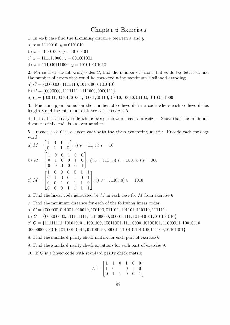
Chapter 6 Exercises1. In each case find the Hamming distance between x and y.

a) x = 1110010, y = 0101010

b) x = 10001000, y = 10100101

c) x = 111111000, y = 001001001

d) x = 111000111000, y = 101010101010

2. For each of the following codes C, find the number of errors that could be detected, andthe number of errors that could be corrected using maximum-likelihood decoding.

a) C = {0000000, 1111110, 1010100, 0101010}b) C = {0000000, 1111111, 1111000, 0000111}c) C = {00011, 00101, 01001, 10001, 00110, 01010, 10010, 01100, 10100, 11000}

3. Find an upper bound on the number of codewords in a code where each codeword haslength 8 and the minimum distance of the code is 5.

4. Let C be a binary code where every codeword has even weight. Show that the minimumdistance of the code is an even number.

5. In each case C is a linear code with the given generating matrix. Encode each messageword.

a) M =

[1 0 1 10 1 1 0

], i) v = 11, ii) v = 10

b) M =

1 0 0 1 0 00 1 0 0 1 00 0 1 0 0 1

, i) v = 111, ii) v = 100, iii) v = 000

c) M =

1 0 0 0 0 1 10 1 0 0 1 0 10 0 1 0 1 1 00 0 0 1 1 1 1

, i) v = 1110, ii) v = 1010

6. Find the linear code generated by M in each case for M from exercise 6.

7. Find the minimum distance for each of the following linear codes.

a) C = {000000, 001001, 010010, 100100, 011011, 101101, 110110, 111111}b) C = {000000000, 111111111, 111100000, 000011111, 101010101, 010101010}c) C = {11111111, 10101010, 11001100, 10011001, 11110000, 10100101, 11000011, 10010110,00000000, 01010101, 00110011, 01100110, 00001111, 01011010, 00111100, 01101001}

8. Find the standard parity check matrix for each part of exercise 6.

9. Find the standard parity check equations for each part of exercise 9.

10. If C is a linear code with standard parity check matrix

H =

1 1 0 1 0 01 0 1 0 1 00 1 1 0 0 1

89

find a generating matrix for C in standard form.

11. Assume that relatively few errors occur and that r = 101001 is received using the codegenerated by the matrix from exercise 6 b). What is the most likely codeword sent?

12. Repeat exercise 11 with r = 001001.

13. Suppose we are using the code generated by M from exercise 6c) and r = 1110110 isreceived. Determine whether an error occured in transmission, and if so determine the mostlikely codeword transmitted.

14. Repeat exercise 13 with r = 1010011.

90

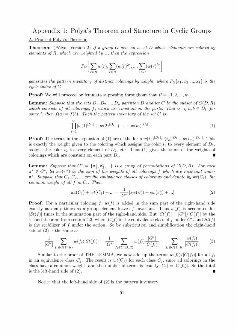
Appendix 1: Po′lya’s Theorem and Structure in Cyclic Groups

A. Proof of Polya’s Theorem:

Theorem: (Polya Version 2) If a group G acts on a set D whose elements are colored byelements of R, which are weighted by w, then the expression

PG

[∑r∈R

w(r),∑r∈R

(w(r)2), ...,∑r∈R

(w(r)k)

]

generates the pattern inventory of distinct colorings by weight, where PG[x1, x2, ..., xk] is thecycle index of G.

Proof: We will proceed by lemmata supposing throughout that R = {1, 2, ...,m}.

Lemma: Suppose that the sets D1, D2, ..., Dp partition D and let C be the subset of C(D,R)which consists of all colorings, f , which are constant on the parts. That is, if a, b ∈ Di, forsome i, then f(a) = f(b). Then the pattern inventory of the set C is

m∏i=1

[w(1)|Di| + w(2)|Di| + ...+ w(m)|Di|] (1)

Proof: The terms in the expansion of (1) are of the form w(i1)|D1|w(i2)

|D2|...w(im)|Dm|. Thisis exactly the weight given to the coloring which assigns the color i1 to every element of D1,assigns the color i2 to every element of D2, etc. Thus (1) gives the sums of the weights ofcolorings which are constant on each part Di.

Lemma: Suppose that G∗ = {π∗1 , π

∗2 , ...} is a group of permutations of C(D,R). For each

π∗ ∈ G∗, let sw(π∗) be the sum of the weights of all colorings f which are invariant underπ∗. Suppose that C1, C2, ... are the equivalence classes of colorings and denote by wt(Ci), thecommon weight of all f in Ci. Then

wt(C1) + wt(C2) + ... =1

|G∗|[sw(π∗

1) + sw(π∗2) + ...] (2)

Proof: For a particular coloring f , w(f) is added in the sum part of the right-hand sideexactly as many times as a group element leaves f invariant. Thus w(f) is accounted for|St(f)| times in the summation part of the right-hand side. But |St(f)| = |G∗|/|C(f)| by thesecond theorem from section 4.3, where C(f) is the equivalence class of f under G∗, and St(f)is the stabilizer of f under the action. So by substitution and simplification the right-handside of (2) is the same as

1

|G∗|∑

fi∈C(D,R)

w(fi)|St(fi)| =1

|G∗|∑

fi∈C(D,R)

w(fi)|G∗||C(fi)|

=∑

fi∈C(D,R)

w(fi)

|C(fi)|(3)

Similar to the proof of THE LEMMA, we now add up the terms w(fi)/|C(fi)| for all fiin an equivalence class Cj . The result is wt(Cj) for each class Cj , since all colorings in theclass have a common weight, and the number of terms is exactly |Cj | = |C(fi)|. So the totalis the left-hand side of (2).

Notice that the left-hand side of (2) is the pattern inventory.

91

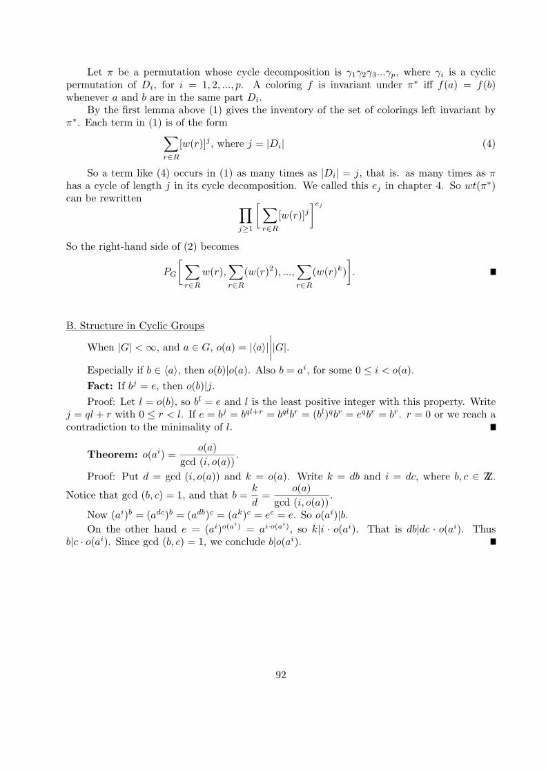
Let π be a permutation whose cycle decomposition is γ1γ2γ3...γp, where γi is a cyclicpermutation of Di, for i = 1, 2, ..., p. A coloring f is invariant under π∗ iff f(a) = f(b)whenever a and b are in the same part Di.

By the first lemma above (1) gives the inventory of the set of colorings left invariant byπ∗. Each term in (1) is of the form∑

r∈R

[w(r)]j , where j = |Di| (4)

So a term like (4) occurs in (1) as many times as |Di| = j, that is. as many times as πhas a cycle of length j in its cycle decomposition. We called this ej in chapter 4. So wt(π∗)can be rewritten ∏

j≥1

[∑r∈R

[w(r)]j]ej

So the right-hand side of (2) becomes

PG

[∑r∈R

w(r),∑r∈R

(w(r)2), ...,∑r∈R

(w(r)k)

].

B. Structure in Cyclic Groups

When |G| <∞, and a ∈ G, o(a) = |⟨a⟩|∣∣∣∣|G|.

Especially if b ∈ ⟨a⟩, then o(b)|o(a). Also b = ai, for some 0 ≤ i < o(a).

Fact: If bj = e, then o(b)|j.Proof: Let l = o(b), so bl = e and l is the least positive integer with this property. Write

j = ql + r with 0 ≤ r < l. If e = bj = bql+r = bqlbr = (bl)qbr = eqbr = br. r = 0 or we reach acontradiction to the minimality of l.

Theorem: o(ai) =o(a)

gcd (i, o(a)).

Proof: Put d = gcd (i, o(a)) and k = o(a). Write k = db and i = dc, where b, c ∈ ZZ.

Notice that gcd (b, c) = 1, and that b =k

d=

o(a)

gcd (i, o(a)).

Now (ai)b = (adc)b = (adb)c = (ak)c = ec = e. So o(ai)|b.On the other hand e = (ai)o(a

i) = ai·o(ai), so k|i · o(ai). That is db|dc · o(ai). Thus

b|c · o(ai). Since gcd (b, c) = 1, we conclude b|o(ai).

92

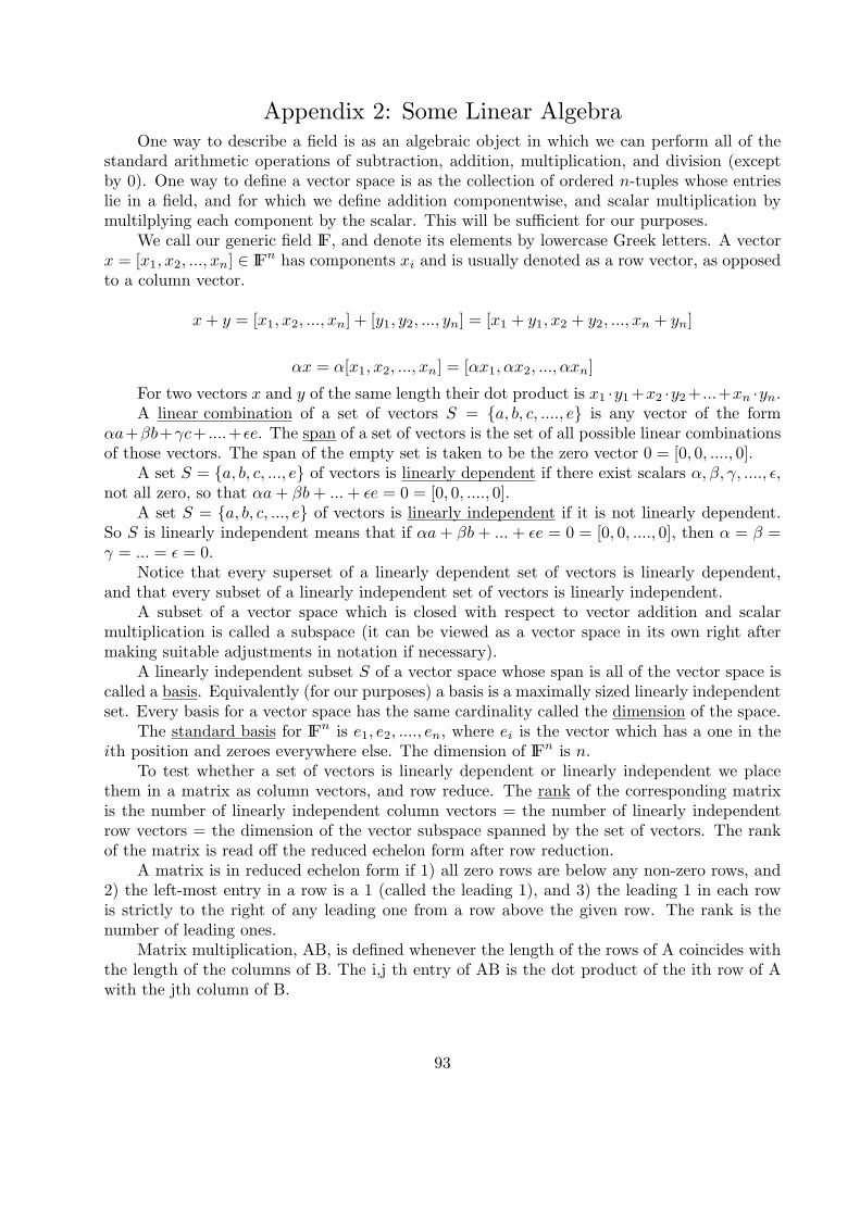
Appendix 2: Some Linear AlgebraOne way to describe a field is as an algebraic object in which we can perform all of the

standard arithmetic operations of subtraction, addition, multiplication, and division (exceptby 0). One way to define a vector space is as the collection of ordered n-tuples whose entrieslie in a field, and for which we define addition componentwise, and scalar multiplication bymultilplying each component by the scalar. This will be sufficient for our purposes.

We call our generic field IF, and denote its elements by lowercase Greek letters. A vectorx = [x1, x2, ..., xn] ∈ IFn has components xi and is usually denoted as a row vector, as opposedto a column vector.

x+ y = [x1, x2, ..., xn] + [y1, y2, ..., yn] = [x1 + y1, x2 + y2, ..., xn + yn]

αx = α[x1, x2, ..., xn] = [αx1, αx2, ..., αxn]

For two vectors x and y of the same length their dot product is x1 ·y1+x2 ·y2+ ...+xn ·yn.A linear combination of a set of vectors S = {a, b, c, ...., e} is any vector of the form

αa+βb+γc+ ....+ϵe. The span of a set of vectors is the set of all possible linear combinationsof those vectors. The span of the empty set is taken to be the zero vector 0 = [0, 0, ...., 0].

A set S = {a, b, c, ..., e} of vectors is linearly dependent if there exist scalars α, β, γ, ...., ϵ,not all zero, so that αa+ βb+ ...+ ϵe = 0 = [0, 0, ...., 0].

A set S = {a, b, c, ..., e} of vectors is linearly independent if it is not linearly dependent.So S is linearly independent means that if αa+ βb+ ...+ ϵe = 0 = [0, 0, ...., 0], then α = β =γ = ... = ϵ = 0.

Notice that every superset of a linearly dependent set of vectors is linearly dependent,and that every subset of a linearly independent set of vectors is linearly independent.

A subset of a vector space which is closed with respect to vector addition and scalarmultiplication is called a subspace (it can be viewed as a vector space in its own right aftermaking suitable adjustments in notation if necessary).

A linearly independent subset S of a vector space whose span is all of the vector space iscalled a basis. Equivalently (for our purposes) a basis is a maximally sized linearly independentset. Every basis for a vector space has the same cardinality called the dimension of the space.

The standard basis for IFn is e1, e2, ...., en, where ei is the vector which has a one in theith position and zeroes everywhere else. The dimension of IFn is n.

To test whether a set of vectors is linearly dependent or linearly independent we placethem in a matrix as column vectors, and row reduce. The rank of the corresponding matrixis the number of linearly independent column vectors = the number of linearly independentrow vectors = the dimension of the vector subspace spanned by the set of vectors. The rankof the matrix is read off the reduced echelon form after row reduction.

A matrix is in reduced echelon form if 1) all zero rows are below any non-zero rows, and2) the left-most entry in a row is a 1 (called the leading 1), and 3) the leading 1 in each rowis strictly to the right of any leading one from a row above the given row. The rank is thenumber of leading ones.

Matrix multiplication, AB, is defined whenever the length of the rows of A coincides withthe length of the columns of B. The i,j th entry of AB is the dot product of the ith row of Awith the jth column of B.

93

Appendix 3: Some Handy Mathematica CommandsA. PolyaCounting

When we have the cycle index of a permutation group we can enter it into Mathematica asa function which we can evaluate and manipulate to more easily take advantage of the patterninventories via weight functions.

For example we might determine that the cycle index of the symmetric group on 4 lettersacting on the edges of K4 is

PS4

[x1, x2, x3, x4

]=

1

24(x6

1 + 6x2x4 + 8x23 + 9x2

1x22)

In Mathematica we would enter

K4[x , y , z , w ] := (1/24)(x6 + 6yw + 8z2 + 9x2y2)

The ’s after x, y, z, w let Mathematica know that these are being declared as variables. Afterdefining this function if we enter K4[2, 2, 2, 2] the output would be the number of ways ofcoloring the edges of K4 using two colors (such as there and not there). If we next give weights1 for not there, and x for there, then enteringK4[1+x, 1+x2, 1+x3, 1+x4] and Expand[%], theresult is the pattern inventory which is the enumeration of isomorphism classes of simple graphson four vertices. Another useful command is one such as Sum[Coefficient[%, xi], {i, 3, 6}],which would sum all coefficients of x3 through x6 in the previous output.

B. Finite Fields

To factor a polynomial modulo an integer m we use Factor[x11 − x,Modulus− > m]. Ofcourse we would probably prefer to define the function g[x ] = x81 − x; and thenFactor[g[x],Modulus− > 3].

This would allow us to find all monic irreducible quartics mod 3 which might be used tobuild GF (81).

To work in GF (81) we need commands such as

Reddus[expr ] := PolynomialMod[PolynomialMod[expr,m/.x− > α], p]

Add[f , g ] := Reddus[f + g]; , and Mult[f , g ] := Reddus[fg];

To determine if (mod 3) a monic irreducible quartic is primitive we would set say p =3;m = x4 + 2x+ 2; and then generate the powers of a root of m, to see if it’s order was 80 ornot.

nonzero = Column[Table[ai, Reddus[ai], i, 0, 80]]

The above logarithmic table would allow us to do computations in the field more efficiently.

C. Matrices

A matrix can be entered into Mathematica as a list of lists, or vector of vectors. Forexample

A := {{1, 0, 0, 0, 1, 1, 1}, {0, 1, 0, 0, 0, 1, 1}, {0, 0, 1, 0, 1, 0, 1}, {0, 0, 0, 1, 1, 1, 0}}; enters thegenerating matrix for a Hamming code of length 7.

Matrix muliplication is done by ., so if A and B are appropriately sized matrices thereproduct is A.B. This works for matrix-vector multiplication as well. Output can be seen in ma-trix form using the command MatrixForm[A.B]. Other useful commands are Transpose[M ],Inverse[A], and RowReduce[M,Modulus− > 2].

94

Appendix 4: GNU Free Documentation LicenseVersion 1.3, 3 November 2008

Copyright 2000, 2001, 2002, 2007, 2008 Free Software Foundation, Inc. <<http://fsf.org/>>

Everyone is permitted to copy and distribute verbatim copies of this license document,but changing it is not allowed.

0. PREAMBLE

The purpose of this License is to make a manual, textbook, or other functional and usefuldocument ”free” in the sense of freedom: to assure everyone the effective freedom to copyand redistribute it, with or without modifying it, either commercially or noncommercially.Secondarily, this License preserves for the author and publisher a way to get credit for theirwork, while not being considered responsible for modifications made by others.

This License is a kind of ”copyleft”, which means that derivative works of the documentmust themselves be free in the same sense. It complements the GNU General Public License,which is a copyleft license designed for free software. We have designed this License in orderto use it for manuals for free software, because free software needs free documentation: a freeprogram should come with manuals providing the same freedoms that the software does. Butthis License is not limited to software manuals; it can be used for any textual work, regardlessof subject matter or whether it is published as a printed book. We recommend this Licenseprincipally for works whose purpose is instruction or reference.

1. APPLICABILITY AND DEFINITIONS

This License applies to any manual or other work, in any medium, that contains a noticeplaced by the copyright holder saying it can be distributed under the terms of this License.Such a notice grants a world-wide, royalty-free license, unlimited in duration, to use thatwork under the conditions stated herein. The ”Document”, below, refers to any such manualor work. Any member of the public is a licensee, and is addressed as ”you”. You accept thelicense if you copy, modify or distribute the work in a way requiring permission under copyrightlaw.

A ”Modified Version” of the Document means any work containing the Document or aportion of it, either copied verbatim, or with modifications and/or translated into anotherlanguage.

A ”Secondary Section” is a named appendix or a front-matter section of the Documentthat deals exclusively with the relationship of the publishers or authors of the Document to theDocument’s overall subject (or to related matters) and contains nothing that could fall directlywithin that overall subject. (Thus, if the Document is in part a textbook of mathematics, aSecondary Section may not explain any mathematics.) The relationship could be a matterof historical connection with the subject or with related matters, or of legal, commercial,philosophical, ethical or political position regarding them.

The ”Invariant Sections” are certain Secondary Sections whose titles are designated, asbeing those of Invariant Sections, in the notice that says that the Document is released underthis License. If a section does not fit the above definition of Secondary then it is not allowedto be designated as Invariant. The Document may contain zero Invariant Sections. If theDocument does not identify any Invariant Sections then there are none.

The ”Cover Texts” are certain short passages of text that are listed, as Front-Cover Textsor Back-Cover Texts, in the notice that says that the Document is released under this License.A Front-Cover Text may be at most 5 words, and a Back-Cover Text may be at most 25 words.

A ”Transparent” copy of the Document means a machine-readable copy, represented in a

95

format whose specification is available to the general public, that is suitable for revising thedocument straightforwardly with generic text editors or (for images composed of pixels) genericpaint programs or (for drawings) some widely available drawing editor, and that is suitablefor input to text formatters or for automatic translation to a variety of formats suitable forinput to text formatters. A copy made in an otherwise Transparent file format whose markup,or absence of markup, has been arranged to thwart or discourage subsequent modification byreaders is not Transparent. An image format is not Transparent if used for any substantialamount of text. A copy that is not ”Transparent” is called ”Opaque”.

Examples of suitable formats for Transparent copies include plain ASCII without markup,Texinfo input format, LaTeX input format, SGML or XML using a publicly available DTD,and standard-conforming simple HTML, PostScript or PDF designed for human modification.Examples of transparent image formats include PNG, XCF and JPG. Opaque formats includeproprietary formats that can be read and edited only by proprietary word processors, SGML orXML for which the DTD and/or processing tools are not generally available, and the machine-generated HTML, PostScript or PDF produced by some word processors for output purposesonly.

The ”Title Page” means, for a printed book, the title page itself, plus such following pagesas are needed to hold, legibly, the material this License requires to appear in the title page.For works in formats which do not have any title page as such, ”Title Page” means the textnear the most prominent appearance of the work’s title, preceding the beginning of the bodyof the text.

The ”publisher” means any person or entity that distributes copies of the Document tothe public.

A section ”Entitled XYZ” means a named subunit of the Document whose title either isprecisely XYZ or contains XYZ in parentheses following text that t ranslates XYZ in anotherlanguage. (Here XYZ stands for a specific section name mentioned below, such as ”Acknowl-edgements”, ”Dedications”, ”Endorsements”, or ”History”.) To ”Preserve the Title” of sucha section when you modify the Document means that it remains a section ”Entitled XYZ”according to this definition.

The Document may include Warranty Disclaimers next to the notice which states that thisLicense applies to the Document. These Warranty Disclaimers are considered to be includedby reference in this License, but only as regards disclaiming warranties: any other implicationthat these Warranty Disclaimers may have is void and has no effect on the meaning of thisLicense.

2. VERBATIM COPYING

You may copy and distribute the Document in any medium, either commercially or non-commercially, provided that this License, the copyright notices, and the license notice sayingthis License applies to the Document are reproduced in all copies, and that you add no otherconditions whatsoever to those of this License. You may not use technical measures to obstructor control the reading or further copying of the copies you make or distribute. However, youmay accept compensation in exchange for copies. If you distribute a large enough number ofcopies you must also follow the conditions in section 3. You may also lend copies, under thesame conditions stated above, and you may publicly display copies.

3. COPYING IN QUANTITY

If you publish printed copies (or copies in media that commonly have printed covers) ofthe Document, numbering more than 100, and the Document’s license notice requires Cover

96

Texts, you must enclose the copies in covers that carry, clearly and legibly, all these CoverTexts: Front-Cover Texts on the front cover, and Back-Cover Texts on the back cover. Bothcovers must also clearly and legibly identify you as the publisher of these copies. The frontcover must present the full title with all words of the title equally prominent and visible. Youmay add other material on the covers in addition. Copying with changes limited to the covers,as long as they preserve the title of the Document and satisfy these conditions, can be treatedas verbatim copying in other respects.

If the required texts for either cover are too voluminous to fit legibly, you should put thefirst ones listed (as many as fit reasonably) on the actual cover, and continue the rest ontoadjacent pages.

If you publish or distribute Opaque copies of the Document numbering more than 100,you must either include a machine-readable Transparent copy along with each Opaque copy,or state in or with each Opaque copy a computer-network location from which the generalnetwork-using public has access to download using public-standard network protocols a com-plete Transparent copy of the Document, free of added material. If you use the latter option,you must take reasonably prudent steps, when you begin distribution of Opaque copies inquantity, to ensure that this Transparent copy will remain thus accessible at the stated lo-cation until at least one year after the last time you distribute an Opaque copy (directly orthrough your agents or retailers) of that edition to the public.

It is requested, but not required, that you contact the authors of the Document wellbefore redistributing any large number of copies, to give them a chance to provide you withan updated version of the Document.

4. MODIFICATIONS

You may copy and distribute a Modified Version of the Document under the conditionsof sections 2 and 3 above, provided that you release the Modified Version under precisely thisLicense, with the Modified Version filling the role of the Document, thus licensing distributionand modification of the Modified Version to whoever possesses a copy of it. In addition, youmust do these things in the Modified Version:

A. Use in the Title Page (and on the covers, if any) a title distinct from that of theDocument, and from those of previous versions (which should, if there were any, be listed inthe History section of the Document). You may use the same title as a previous version ifthe original publisher of that version gives permission. B. List on the Title Page, as authors,one or more persons or entities responsible for authorship of the modifications in the ModifiedVersion, together with at least five of the principal authors of the Document (all of its principalauthors, if it has fewer than five), unless they release you from this requirement. C. Stateon the Title page the name of the publisher of the Modified Version, as the publisher. D.Preserve all the copyright notices of the Document. E. Add an appropriate copyright noticefor your modifications adjacent to the other copyright notices. F. Include, immediately afterthe copyright notices, a license notice giving the public permission to use the Modified Versionunder the terms of this License, in the form shown in the Addendum below. G. Preservein that license notice the full lists of Invariant Sections and required Cover Texts given inthe Document’s license notice. H. Include an unaltered copy of this License. I. Preserve thesection Entitled ”History”, Preserve its Title, and add to it an item stating at least the title,year, new authors, and publisher of the Modified Version as given on the Title Page. If thereis no section Entitled ”History” in the Document, create one stating the title, year, authors,and publisher of the Document as given on its Title Page, then add an item describing the

97

Modified Version as stated in the previous sentence. J. Preserve the network location, if any,given in the Document for public access to a Transparent copy of the Document, and likewisethe network locations given in the Document for previous versions it was based on. Thesemay be placed in the ”History” section. You may omit a network location for a work thatwas published at least four years before the Document itself, or if the original publisher ofthe version it refers to gives permission. K. For any section Entitled ”Acknowledgements” or”Dedications”, Preserve the Title of the section, and preserve in the section all the substanceand tone of each of the contributor acknowledgements and/or dedications given therein. L.Preserve all the Invariant Sections of the Document, unaltered in their text and in their titles.Section numbers or the equivalent are not considered part of the section titles. M. Delete anysection Entitled ”Endorsements”. Such a section may not be included in the Modified Version.N. Do not retitle any existing section to be Entitled ”Endorsements” or to conflict in title withany Invariant Section. O. Preserve any Warranty Disclaimers.

If the Modified Version includes new front-matter sections or appendices that qualify asSecondary Sections and contain no material copied from the Document, you may at your optiondesignate some or all of these sections as invariant. To do this, add their titles to the list ofInvariant Sections in the Modified Version’s license notice. These titles must be distinct fromany other section titles. You may add a section Entitled ”Endorsements”, provided it containsnothing but endorsements of your Modified Version by various partiesfor example, statementsof peer review or that the text has been approved by an organization as the authoritativedefinition of a standard. You may add a passage of up to five words as a Front-Cover Text,and a passage of up to 25 words as a Back-Cover Text, to the end of the list of Cover Textsin the Modified Version. Only one passage of Front-Cover Text and one of Back-Cover Textmay be added by (or through arrangements made by) any one entity. If the Document alreadyincludes a cover text for the same cover, previously added by you or by arrangement made bythe same entity you are acting on behalf of, you may not add another; but you may replacethe old one, on explicit permission from the previous publisher that added the old one. Theauthor(s) and publisher(s) of the Document do not by this License give permission to use theirnames for publicity for or to assert or imply endorsement of any Modified Version.

5. COMBINING DOCUMENTS

You may combine the Document with other documents released under this License, underthe terms defined in section 4 above for modified versions, provided that you include in thecombination all of the Invariant Sections of all of the original documents, unmodified, andlist them all as Invariant Sections of your combined work in its license notice, and that youpreserve all their Warranty Disclaimers.

The combined work need only contain one copy of this License, and multiple identicalInvariant Sections may be replaced with a single copy. If there are multiple Invariant Sectionswith the same name but different contents, make the title of each such section unique byadding at the end of it, in parentheses, the name of the original author or publisher of thatsection if known, or else a unique number. Make the same adjustment to the section titles inthe list of Invariant Sections in the license notice of the combined work.

In the combination, you must combine any sections Entitled ”History” in the variousoriginal documents, forming one section Entitled ”History”; likewise combine any sectionsEntitled ”Acknowledgements”, and any sections Entitled ”Dedications”. You must delete allsections Entitled ”Endorsements”.

6. COLLECTIONS OF DOCUMENTS

98

You may make a collection consisting of the Document and other documents releasedunder this License, and replace the individual copies of this License in the various documentswith a single copy that is included in the collection, provided that you follow the rules of thisLicense for verbatim copying of each of the documents in all other respects.

You may extract a single document from such a collection, and distribute it individuallyunder this License, provided you insert a copy of this License into the extracted document,and follow this License in all other respects regarding verbatim copying of that document.

7. AGGREGATION WITH INDEPENDENT WORKS

A compilation of the Document or its derivatives with other separate and independentdocuments or works, in or on a volume of a storage or distribution medium, is called an”aggregate” if the copyright resulting from the compilation is not used to limit the legal rightsof the compilation’s users beyond what the individual works permit. When the Documentis included in an aggregate, this License does not apply to the other works in the aggregatewhich are not themselves derivative works of the Document.

If the Cover Text requirement of section 3 is applicable to these copies of the Document,then if the Document is less than one half of the entire aggregate, the Document’s Cover Textsmay be placed on covers that bracket the Document within the aggregate, or the electronicequivalent of covers if the Document is in electronic form. Otherwise they must appear onprinted covers that bracket the whole aggregate.

8. TRANSLATION

Translation is considered a kind of modification, so you may distribute translations ofthe Document under the terms of section 4. Replacing Invariant Sections with translationsrequires special permission from their copyright holders, but you may include translations ofsome or all Invariant Sections in addition to the original versions of these Invariant Sections.You may include a translation of this License, and all the license notices in the Document, andany Warranty Disclaimers, provided that you also include the original English version of thisLicense and the original versions of those notices and disclaimers. In case of a disagreementbetween the translation and the original version of this License or a notice or disclaimer, theoriginal version will prevail. If a section in the Document is Entitled ”Acknowledgements”,”Dedications”, or ”History”, the requirement (section 4) to Preserve its Title (section 1) willtypically require changing the actual title.

9. TERMINATION

You may not copy, modify, sublicense, or distribute the Document except as expresslyprovided under this License. Any attempt otherwise to copy, modify, sublicense, or distributeit is void, and will automatically terminate your rights under this License.

However, if you cease all violation of this License, then your license from a particularcopyright holder is reinstated (a) provisionally, unless and until the copyright holder explicitlyand finally terminates your license, and (b) permanently, if the copyright holder fails to notifyyou of the violation by some reasonable means prior to 60 days after the cessation.

Moreover, your license from a particular copyright holder is reinstated permanently if thecopyright holder notifies you of the violation by some reasonable means, this is the first timeyou have received notice of violation of this License (for any work) from that copyright holder,and you cure the violation prior to 30 days after your receipt of the notice.

Termination of your rights under this section does not terminate the licenses of parties whohave received copies or rights from you under this License. If your rights have been terminatedand not permanently reinstated, receipt of a copy of some or all of the same material does not

99

give you any rights to use it.

10. FUTURE REVISIONS OF THIS LICENSE

The Free Software Foundation may publish new, revised versions of the GNU Free Docu-mentation License from time to time. Such new versions will be similar in spirit to the presentversion, but may differ in detail to address new problems or concerns. See

http://www.gnu.org/copyleft/.

Each version of the License is given a distinguishing version number. If the Documentspecifies that a particular numbered version of this License ”or any later version” applies to it,you have the option of following the terms and conditions either of that specified version or ofany later version that has been published (not as a draft) by the Free Software Foundation. Ifthe Document does not specify a version number of this License, you may choose any versionever published (not as a draft) by the Free Software Foundation. If the Document specifiesthat a proxy can decide which future versions of this License can be used, that proxy’s publicstatement of acceptance of a version permanently authorizes you to choose that version for theDocument.

11. RELICENSING

”Massive Multiauthor Collaboration Site” (or ”MMC Site”) means any World Wide Webserver that publishes copyrightable works and also provides prominent facilities for anybodyto edit those works. A public wiki that anybody can edit is an example of such a server.A ”Massive Multiauthor Collaboration” (or ”MMC”) contained in the site means any set ofcopyrightable works thus published on the MMC site.

”CC-BY-SA” means the Creative Commons Attribution-Share Alike 3.0 license publishedby Creative Commons Corporation, a not-for-profit corporation with a principal place of busi-ness in San Francisco, California, as well as future copyleft versions of that license publishedby that same organization. ”Incorporate” means to publish or republish a Document, in wholeor in part, as part of another Document.

An MMC is ”eligible for relicensing” if it is licensed under this License, and if all worksthat were first published under this License somewhere other than this MMC, and subsequentlyincorporated in whole or in part into the MMC, (1) had no cover texts or invariant sections,and (2) were thus incorporated prior to November 1, 2008.

The operator of an MMC Site may republish an MMC contained in the site under CC-BY-SA on the same site at any time before August 1, 2009, provided the MMC is eligible forrelicensing.

ADDENDUM: How to use this License for your documents

To use this License in a document you have written, include a copy of the License in thedocument and put the following copyright and license notices just after the title page:

Copyright (C) YEAR YOUR NAME. Permission is granted to copy, distribute and/ormodify this document under the terms of the GNU Free Documentation License, Version 1.3or any later version published by the Free Software Foundation; with no Invariant Sections, noFront-Cover Texts, and no Back-Cover Texts. A copy of the license is included in the sectionentitled ”GNU Free Documentation License”.

If you have Invariant Sections, Front-Cover Texts and Back-Cover Texts, replace the ”withTexts.” line with this:

with the Invariant Sections being LIST THEIR TITLES, with the Front-Cover Textsbeing LIST, and with the Back-Cover Texts being LIST.

If you have Invariant Sections without Cover Texts, or some other combination of the

100

three, merge those two alternatives to suit the situation.If your document contains nontrivial examples of program code, we recommend releasing

these examples in parallel under your choice of free software license, such as the GNU GeneralPublic License, to permit their use in free software.

back to top Check out other Free Software Foundation campaignsDefective by Design <http://defectivebydesign.org/>, a campaign against Digital Re-

strictions Management (DRM) Windows 7 Sins <http://windows7sins.org/>, the case againstMicrosoft and proprietary software PlayOgg <http://playogg.org/> support free media for-mats Please send FSF & GNU inquiries to gnu@gnu.org <mailto:gnu@gnu.org>. There arealso other ways to contact </contact/> the FSF.

Please send broken links and other corrections or suggestions to webmasters@gnu.org<mailto:webmasters@gnu.org>.

Please see the Translations README </server/standards/README.translations.html>for information on coordinating and submitting translations of this article.

Copyright notice above.51 Franklin Street, Fifth Floor, Boston, MA 02110, USAVerbatim copying and distribution of this entire article is permitted in any medium with-

out royalty provided this notice is preserved.Updated: Date : 2009/06/1719 : 20 : 31Translations of this pageEnglish </licenses/fdl-1.3.html> [en]

101