Mathematical Analysis and Numerical Methods for Science and Technology || The Linearised Navier-Stokes Equations

Chapter XIX. The Linearised Navier-Stokes Equations

Introduction

The object ofthis chapter is to present a certain number ofresults on the linearised Navier-Stokes equations. The Navier-Stokes equations, which describe the motion of a viscous, incompressible fluid were introduced already, from the physical point of view, in §1 of Chap. IA. These equations are nonlinear. We study here the equations that emerge on linearisation from the solution (u = 0, p = 0). This is an interesting exercise in its own right. It corresponds to the case of a very slow flow, and also prepares the way for the study of the complete Navier-Stokes equations. This Chap. XIX is made up of two parts, devoted respectively to linearised stationary equations (or Stokes' problem), and to linearised evolution equations. Questions of existence, uniqueness, and regularity of solutions are considered from the variational point of view, making use of general results proved elsewhere. The functional spaces introduced for this purpose are themselves of interest and are therefore studied comprehensively.

§ 1. The Stationary Navier-Stokes Equations: The Linear Case

Orientation: Presentation of Stationary Problem

The motion of a homogeneous, viscous, incompressible fluid is described by the Navier-Stokes equations. These have been introduced in §1 of Chap. IA. Here, we shall study the Navier-Stokes equations in the case of a stationary (or permanent) flow after linearisation. It is therefore the Stokes problem which will be considered, i.e.: determine the velocity u = (Ub ... , unP) and the pressure p, in a domain a, such that:

(1)

(2)

(3)

- vLlu + grad p = f in a, a c IRn(v > 0)(2)

div u = 0 in a, u = 0 over aa.

(I) Also denoted by U in Chap. I A, §l. (2) We take the space IR" in order to treat simultaneously the usual cases n = 2 and n = 3

R. Dautray et al., Mathematical Analysis and Numerical Methods for Science and Technology

© Springer-Verlag Berlin Heidelberg 2000

2 Chapter XIX. The Linearised Navier-Stokes Equations

The boundary conditions, u = 0 on oQ, correspond to the case of a rigid boundary oQ with the fluid adhering to it. The approach to problem (1H3) will be variational. Some function spaces adapted to the problem will be introduced (Sect. 1), which will allow us to pose a weak form equivalent to (1), (2), (3). The existence and uniqueness (Sect. 2) of the solution then follows from the Lax-Milgram theorem(3). After a study for bounded Q, these results will be extended to cases of problems which are totally nonhomogeneous, with unbounded domain Q and to the study of eigenvalue problems. We also demonstrate the interest of the concept of penalisation. The delicate question of regularity in broached in Sect. 3.

1. Functional Spaces

1.1. Notation

Let Q be an open set of the Euclidean space IRn. In what follows two types of regularity hypotheses will be used on Q. A strong hypothesis:

(1.1) { the boundary r of Q is a manifold of dimension (n - 1) of class ~r (r precisely) and Q is locally situated on one side of r .

We say that Q satisfying (1.1) is of class ~r. The second hypothesis is less restrictive (if r ? 1):

{ the boundary r of Q is locally Lipschitz, i.e. is represented (1.2) locally by the graph of a Lipschitz function(4) .

If Q satisfies (1.2), it is then locally star-shaped, i.e. every point x of r has a neighbourhood (!J such that (!J n Q is star-shaped with respect to one of its points (Necas [1], [2]). Our definition ofa star-shaped open set is a little more restrictive than the usual definition: we say that (!J is star-shaped with respect to the origin if A& c: (!J for all A, 0 ~ A < 1. We further assume that all of the open sets Q of this Chap. XIX are connected. With every open set Q we associate the usual spaces '@(Q) (and '@(Q)), U(Q), and the Sobolev spaces wm,a(Q) (m an integer and 1 ~ IX ~ + 00 ), all equipped with their usual norms. If IX = 2, we set w m, 2 (Q) = H m( Q). The closure of '@(Q) in wm,a(Q) will be denoted W;j',a(Q) (H;j'(Q) if IX = 2). For convenience, due to the frequent use of vector-valued functions with n components in what follows, we shall use the following notation in this chapter:

§j (Q) = ['@(Q)]n, lLa(Q) = [L a(Q)]n ,

wm,a(Q) = [wm.a(Q)y, IHJm(Q) = [Hm(Q)]n.

All of these spaces (with the exception of ~(Q)) are equipped with the natural

(3) See Chap. VI and VII. (4) We then say that Q is an open Lipschitz set.

§1. The Stationary Navier-Stokes Equations: The Linear Case 3

product norm. Constant use will be made of the following spaces:

L2(Q), IL 2(Q), H 6(Q), IHl6(Q).

The scalar product and the norm of L 2(Q) or IL 2(Q) will be denoted (.,.) and 1.1 (and [.,.], [.] for H6(Q) or IHl6<Q)). Thanks to Poincare's inequality (see Chap. IV), if the open set Q is bounded in one direction, the norm [.] over H 6(Q) (or IHl6(Q)) is equivalent to the norm:

(1.3) II U II = [itt I DiU 12 J/2 (S) •

With the norm (1.3) we associate the scalar product:

n

(1.4) ((u, v)) = L (DiU, Div), i= t

for which the space H 6(Q) (or IHl6(Q)) is also Hilbertian. Equation (2) justifies the introduction of the space (without topology):

(1.5) "1/= {uE5j(Q);divu=O},

and its closures H and V in IL 2(Q) and 1Hl6(Q), which will now be characterised. All of these spaces will be taken to be real in this Chap. XIX.

1.2. A Density Theorem

The auxiliary space E(Q) = {u Ell 2(Q); div U E L 2(Q)} is a Hilbert space equipped with the scalar product

(1.6) ((U, V))E(Q) = (u, v) + (div u, div v),

and the associated norm:

(1.7) II U IIE(Q) = ((u, u))~;~) .

The establishment of a trace theorem for E(Q) functions requires a density result.

Theorem 1(6): Let Q be an open Lipschitz set of ~n. Then the set of vector-valued functions 5j(Q) is dense in E(Q).

Proof Let U be an element of E(Q). We must show that U is the limit in E(Q) of a sequence of functions in 5j(Q). (i) It is always possible to further assume that U has bounded support. In effect, let 0, let <Pa be the restriction to Q of the function x -+ <p(x/a). Then the function <Pau has compact support, belongs to E(Q) and converges to u in this space as a -+ 00. In other words the set of functions of E(Q) with bounded support constitute a dense subspace of E(Q).

(5) We denote D; = iJ/iJx;, 1 ,,; i ,,; n. (6) Theorem 1 and also Theorems 2 and 3 which follow have already been treated in the context of electromagnetism in Chap. IX A, §l, Theorem \, by other methods.


(ii) The case where Q = W. Let U E E([R"), with compact support following point (i). The result is obtained by regularisation by convolution. Let p be a positive function of !iJ([R") such that

r p(x) dx = 1 with which we associate the function p,: x --+ [;-" p(x/[;), O:!( [;:!( 1. Jw The sequence of functions p, * U have the necessary properties: p, * U E !iJ([R") since U has compact support and p, * U converges to U in E([R") as [; --+ 0 by the construction and since div (p, * u) = p, * div u. (iii) The case where Q #- W. From (i), we can always assume that Q is compact. Since Q is Lipschitz it is locally star-shaped; therefore there exists a finite family of open star-shaped sets {(9j LEJ such that Q, {(9jLEJ constitutes an open covering of Q. Let cP, {cpjLEJ be the partition of unity associated with this covering; we have:

(1.8) {u = cpu + L CPjU

jEJ

1 = cP + L CPJ with cP E !iJ(Q) , CPj E !iJ«(9j) . JEJ

The function cpu has compact support in Q, its extension cpu = cpu in Q and o elsewhere, belongs to E([R"). We are therefore reduced to case (ii). We now consider the more delicate case of a function Uj = CPjU (not identically zero). The set (9) = Q n (9j is star-shaped with respect to one of its points which we can assume (via translation) to be the origin O. Let (J;.., A#-O be the homothetic transformation x --+ Ax. Since (9) is Lipschitz and star-shaped with respect to 0:

We assume that the following property has been proved:

(1.9)

where (J;..Uj denotes the function x --+ Uj«(J;..(x)). Let ..1.>1; if t/!jE!iJ(r;..-.(9j) and satisfies 'l'j= 1 in (9j,t/!j«(JAUj) has compact support and belongs to E(W). Since from (1.9) it is sufficient to approximate 'l'j«(JAuj)lo instead of CPjU, we are therefore reduced to case (ii). Property (1.9) follows from the following lemma.

Lemma 1. Let (9 be an open set of[R" which is star-shaped with respect to the origin O.

(i) If P E !iJ'«(9), then (JAP is defined in !iJ'«(JA-.(9) by:

(1.10) < (JAP, lp) = A -n<p, (JA-'lp) , Vlp E !iJ«(JA-.(9), 1 > A> 0(7).

(7) The bracket <. , . > denotes the duality !J&', !J&.


The derivatives of (J A P are linked to the derivatives of p by the formula:

(1.11)

As A --+ 1, A < 1, the restriction of (JAP to (!) converges in the sense of distributions to p. (ii) lfp E L"((!), 1 ~ rx < + 00, then (JAP E L"((JA-1(!) As A --+ 1, A < 1, the restriction of (J AP to (!) converges in L"( (!) to p.

Proof (i) The mapping ¢ --+ A -" < p, (J A-I ¢) is linear and continuous over ~((J A (!): it defines a distribution denoted (J AP, Formula (1.11) follows from (1.10) and from the derivative of a distribution. Let qJ E ~((!); as A --+ 1, A < 1, (JA -I ¢ has compact support contained in (!) and converges to ¢ in ~((!) as A --+ 1. We can then finish, thanks to (1.10). (ii) It is clear that:

II (JAP IIL'(<T"l'J) = A -a II P II L'(l'J) •

It is sufficient therefore to show (ii) restricting ourselves to a dense subspace of L"( (!), for example ~((!) for which the result is immediate. 0

1.3. A Trace Theorem: The Generalised Stokes Formula

We assume at present that Q is an open bounded set of class C(j2. We have here a trace theorem for E(Q) functions which is the analogue of a well-known result (Chap. IV, §4) for H l(Q) functions; there exists a surjective, linear, continuous operatof)'o E !£(H 1 (Q), H 1/2(r» such that You = restriction of u to r if u E ~(Q} Further Yo has a right inverse t Q which is linear and continuous.

Theorem 2. Let Q be an open bounded set of class C(j 2 (8) and let v be the outward normal to r. Then there exists a continuous linear operator Yv E !£(E(Q), H - 1/2(r»

such that:

( 1.12) Yvu = the restriction of u. v to r, Vu E ~(Q) .

The following generalised Stokes formuld 9 ) has a meaning,for all u E E(Q) and all wEH1(Q):

(1.13) (u, grad w) + (div u, w) = <Yvu, Yow) .

Proof Let ¢ E H 1/2(r) and let WE HI (Q) such that YoW = ¢. For u E E(Q), consider the functional:

Xu(qJ)~ f }div u(x)w(x) + u(x).grad w(x)] dx

= (div u, w) + (u, grad w) .

(8) The Theorem remains true if the boundary of Q is only Lipschitz. (9) The terminology "Green's formula" is also used. See Iyanaga-Kawada [I]. p. 97, and Chap. IX A, Chap. XXI.


The proof consists of two lemmas which make precise the properties of X u( </J).

Lemma 2. Xu(</J) is independent of the choice ofw provided that wEHI(Q) with Yow = </J.

Proof Let WI and W2 be two elements of HI (Q) with Yo WI = Yo W2 = </J; let W = WI - W2. We have to prove:

(div u, wd + (u, grad wd = (div u, W2) + (u, grad W2)

that is to say:

(1.14) (div u, w) + (u, grad w) = ° . But w E H I(Q) and Yo w = 0, that is W E H 6(Q): W is therefore the limit in HI (Q) of a sequence {Wm}mEN of E0(Q) functions. But (1.14) is obvious for W replaced by Wm and remains true in the passage to the limit. 0

Now, let W = t Qcp (see above): from the Cauchy-Schwarz inequality and the continuity of t Q (we denote by Co the norm of t Q):

(1.15) IXu(cp)1 ~ IluIIE(Q)llwIIH1(Q)~ Co IluIIE(Q)llcpIIH'''(r) . The linear form </J -+ Xu(</J) is therefore continuous over HI/2(r) and there exists g = g(u) E H- 1/2(r) such that:

( 1.16)

The mapping U -+ g(u) is clearly linear and from (1.15):

(1.17)

which proves that the mapping u -+ g(u) = YvU is linear and continuous from E(Q) into H -1/2(r). The Stokes formula (1.13) is an immediate consequence of the definition g(u) = YvU. It remains to prove (1.12).

Lemma 3. If u E ~(Q), then: YvU is the restriction of u. v to F.

Proof Let u E ~(Q) and WE E0(Q); the Stokes formula for regular functions allows us to write:

Xu(YoW) = fndiV(UW)dX= frW(U.V)dF

= f)U.V)(YOW)dF= <u,v,Yow).

Since Yo(E0(Q)) is dense in H 1/2(r), the relation:

( 1.18)

is obtained by continuity for all </J E HI/2(r). By comparing (1.18) with (1.16) we obtain (1.12). 0

Remark 1. Theorem 1, combined with Lemma 3, assures us that the operator Yv is the unique extension to E(Q) of the mapping U -+ u. v II defined for U E ~(Q). 0

§l. The Stationary Navier-Stokes Equations: The Linear Case 7

Remark 2. We can verify that the operator Y. is in fact surjective from E(Q) into H -1/2(r) and therefore has a right inverse which is linear and continuous. 0

The following theorem characterises Eo(Q), the closure of !e(Q) in E(Q).

Theorem 3. The kernel of Y. coincides with Eo(Q).

Proof Let uEEo(Q); there exists a sequence {Um}meN, UmE~(Q)', which converges to u in E(Q) as m -+ 00. The continuity of the mapping Y. (Theorem 2)

implies that Y.u = lim Y.Um = 0, since Y.Um = O.

Conversely, we show that if U E E(Q) and Y.U = 0, then U is the limit in E(Q) of a sequence of functions in ~(Q). Let 4> E .@(~n) and 4> = 'PIa. By hypothesis Y.u = 0 and (Y.u, Yo4» = 0, which means:

Therefore:

L [(div u). + u.grad4>]dx = 0, '14> E .@(~n), JR"

,,--.J i.e. div U = div U ,

where w = w in Q and 0 elsewhere. Therefore U E E(~n). By proceeding as for the proof of Theorem 1, stages i) and ii) (Q is bounded of class q;2 therefore Lipschitz), by partition of unity, it is always possible to reduce the problem to the case where U has support in (!}j n Q. For such a function u we remark that U, the extension of u by 0, belongs to E(W) and that eT;.u has compact support in {!}j if 0 < A. < 1 ({!}j is star-shaped by hypothesis). Thanks to Lemma 1, eT;.ul(!)j converges to u in E({!}j) (or E(Q)) as A. -+ 1. Consequently, it is sufficient to approximate a function u with compact support in Q by functions of ~(~n), which is obvious by regularisation. 0

1.4. Characterisation of the spaces H and V

Recall the notation of §1.1,

"Y = {u E .@(Q);div u = O}

H = closure of "Y in n.. 2(Q)

V = closure of "Y in IHJA(Q) .

Let Q be an open set of ~n. If p is a distribution over Q and if v E "Y, it is easy to verify that:

(1.19) (gradp, v) = -(p,divv)=O.

The reciprocal of this property is true. This is an essential result for the interpretation of the variational formulation of the Navier-Stokes equations (see §2.3.1). More precisely, we state


Proposition 1. Let Q be an open set off7in and letf = (fl, ... ,In) where/; E E&'(Q), 1 ~ i ~ n. Then f is the gradient of a distribution, that is to say

(1.20) f = gradp for p E E&'(Q) ,

if and only if f satisfies:

(1.21 ) </,v)=O, VVE"Y.

Proof The implication (1.20) => (1.21) has already been proved. The converse implication relies on a deep theorem of de Rham [I] and is omitted. 0

The following proposition makes precise the properties of the gradient operator, and by passage to the adjoint, of the divergence operator. Recall that for bounded Q, L 2(Q)/1R is isomorphic to a subspace of L 2(Q) which is orthogonal to constants, that is

L2(Q)/1R = {p E L2(Q), L p(x) dx = o}. Proposition 2. Let Q be an open, bounded, Lipschitz set of IRn. i) If a distribution p has all of its first derivatives DiP, 1 ~ i ~ n, in L 2(Q), then pEL 2(Q) and:

(1.22) II p II L2(Q)/R ~ C( Q) II grad p II U(Q) •

ii) If a distribution p has all of its first derivatives DiP, 1 ~ i ~ n in H -1 (Q), then pEL 2(Q) and:

(1.23) IlpIIL2(Q)/R ~ C(Q)llgradpIIH-l(Q)'

iii) In the two preceding cases, ifQ is an arbitrary open set oflRn, p is only in Lfoc(Q). Proof Properties i) and (1.22) are proved in Deny-Lions [1] for certain classes of open sets and in particular for open star-shaped sets. If Q is a bounded Lipschitz open set then it is locally star shaped, and with the help of the partition of unity used in the proof of Theorem 1, we are reduced to the case of open star shaped sets. Properties ii) and (1.23) are established by Magenes-Stampacchia [1] for an open set of class CIJ 1 and by Necas [2] under the present hypotheses. When Q has no regularity properties, the preceding results are applicable to every ball whose closure is contained in Q; therefore p E Lfoc(Q). 0

We can now characterise the space H and its orthogonal complement H.1 in L 2(Q).

Theorem 4. (Characterisation of H). Let Q be an open bounded Lipschitz set of IRn. Then:

(1.24)

(1.25)

Proof

H.1 = {uEIL2(Q);U = grad p,pEH 1(Q)},

H= {uEIL2(Q);divu=0,yvu=0}.

i) Proof of (1.24). Let u = grad p where p E HI (Q), then for all v E "Y

(1.26) (u, v) = (grad p, v) = - (p, div v) = 0 .

Therefore u E H.1.


Conversely, let U E H 1- and show that it is the gradient of a function p of HI (Q). By definition, since U E H1-, (u, v) = 0 for all v E "Y. By Proposition 1, U = Vp where p E ~'(Q), and by Proposition 2, p in fact belongs to H I(Q). ii) Proof of (1.25). Let H* = {u E 1L2(Q); div U = 0, YvU = O}, we firstly show that H c H *. Let U E H; then, by definition, U = lim Urn, Urn E "Y. The convergence is in

rn~oo

IL 2(Q), therefore in ~'(Q). Since differentiation is a continuous operation in ~ '(Q) and since div Urn = 0, we see that div U = O. Therefore div Urn = div U = 0; Urn and U therefore belong to E(Q) and

0·27) II U - Urn IIE(!I) = II U - Urn Ill2(Q),

so that Urn converges to U in E(Q). But

YvU = lim YvUrn = lim Urn. vi, = 0 SInce Urn E V. m-+oo m-+oo

Finally U E H *. We assume that H does not coincide with H * and let H ** be the orthogonal complement of H in H*. From (1.24), every U E H** is the gradient of a function p of H I(Q); further p satisfies:

( 1.28) Ll p - div U = 0, u. v I, = :~ I, = 0 .

Consequently, p is a constant and U == O. Therefore H** = {O} and H = H*. 0

Theorem 5. (Decomposition of IL 2(Q)) Let Q be an open bounded set of class C(f2. Then:

(1.29)

where H, HI, H 2 are pairwise orthogonal spaces and

(1.30)

(1.31)

HI = {u E IL 2 (Q); U = grad p, p E HI (Q), Ll P = O}

H 2 = {u E IL 2(Q); U = grad p, p E H MQ)} .

Proof It is clear that HI and H 2 are included in H 1- and that the pairwise intersection of the spaces H, HI, H 2 is reduced to {O}. The spaces HI and H 2 are orthogonal. Indeed, let U = grad p E HI and v = grad q E H 2 ; U E E(Q) and from the generalised Stokes formula (1.13):

(u, v) = (u, grad q) = <y,.u, Yoq) - <q, div u) = 0

since Yoq = 0 and div U = Llp = O. It remains to show that every element U of IL 2(Q) can be written as a sum of elements Uo, Ul, U2 of H, HI, H 2' Let U E IL 2(Q) and let p be the unique solution of the Dirichlet problem

and set:

(1.32) U2 = grad p .


Consider the Neumann problem

(1.33) Aq = 0, Oql = Yv(u - gradp). OV r

We note that div(u - grad p) = 0, so that u - grad p belongs to E(Q); Yv(u - grad p) is therefore an element of H - I/Z(T) and the Stokes formula ensures that:

< Yv(u - grad p), 1) = L div(u - grad p)dx = 0 .

From a result of Lions-Magenes [1] (see also Lions [1], Necas [1]) the Neumann problem (1.33) has a unique solution q up to an additive constant. We then set:

(1.34)

(1.35)

UI = grad p ,

It remains to show that Uo E H. But

div Uo = div(u - UI - uz) = div U - Ap = 0

and

oq YvUo = Yv(u - UI - U2) = Yv(u - grad p) - ov = 0 .

Theorem 6. (Characterisation of V). Let Q be an open Lipschitz set. Then

(1.36) V = {u E IH16(Q), div U = O} .

Proof Let V- = {u E IHIMQ), div U = O}.

o

It is clear that V c V·; indeed if U E V, U = lim Urn, Urn E 1/, in IHIMQ) and it follows

that

lim div Urn = div U = 0 since div Urn = 0 . rn~oo

We shall show that every continuous linear form Lover V· which is null over V is in fact identically null. It will follow that V = V·. Firstly, L has the following (nonunique) representation:

• (1.37) L(v) = I <li,Vi), liEH-I(Q).

i = I

Indeed, since V· is a closed subspace of 1H16(Q), every continuous linear form over V· can be extended to a continuous linear form over IHIMQ) (Hahn-Banach Theorem) which is therefore of the form (1.37). The vector-valued distribution I = (II, ... , I.) belongs to IHI- I (Q) and satisfies • I < Ii, Vi) = 0, \:Iv E 1/. Propositions 1 and 2 are therefore applicable and show that i


I = grad p, P E L2(Q); from which, for all v E IHI~(Q):

n n n

L <Ii, Vi) = I <DiP, Vi) = - L <p, DiVi) = - <p, div V). i i

Now for V E V· n

L(v) = L <Ii, Vi) = - <p, div V) = 0 . i

that is to say L == 0 over V·. o Remark 3. Propositions 1 and 2, Theorems 6 and 5, will be frequently used in what follows. 0

The decomposition result of Theorem 5 can be made more precise by introducing the curl operator (see Chap. IX). Such a decomposition is not necessary for the variational approach laid out here, but is particularly important for numerical applications. 0

2. Existence and Uniqueness Theorem

2.1. Weak Formulation of the Problem and its Equivalence with the Classical Formulation

Let Q be an open bounded set of IRn with boundary r and let! Ell 2(Q). We look for a vector valued function U = (Ul' ... , un) representing the velocity of the fluid and a scalar function p representing the pressure, defined in Q and satisfying the following equations and boundary conditions:

(1.38)

(1.39)

(1.40)

-vLlu+gradp=! inQ(v>O).

div U = 0 in Q ,

U = 0 on r (v is the coefficient of kinematic viscosity which is assumed constant). Iff, u, pare regular functions (for example of class rc 2 in Q) satisfying the classical formulation (1.38H1.40), by multiplying (1.38) by a function v E "Y, we obtain after integration by parts(lO):

n

(f, v) = ( - vLlu + grad p, v) = v L (grad Ui, grad vd - (p, div v) i

= v((u, v))

since div v = o. Therefore,

(1.41 ) v((U, v)) = (f, v), Vv E "Y.

(10) See the notation at the end of § 1.1.


Each side of (1.41) depends linearly and continuously on v for the topology of IHl6(Q); the equation (1.41) is consequently true for all v in V, the closure of "Y in IHl6(Q). If Q is of class C(j 2, then (1.40) assures us that the (regular) function u belongs to IHl6(Q); Theorem 6 and (1.39) ensures that u E V. Finally,

(1.42) u belongs to V and satisfies v«u, v» = (f, v), Vv E V.

Conversely, let u satisfy (1.42); we show that u satisfies (1.38H1.40) in an appropriate sense (certainly more weak than the classical sense, since u only belongs to IHl6(Q». Since u = (Ul' ... , un) E IHl6(Q), the traces 'YOUi are null in H 1/2(r); since u E V, div u is null in ~'(Q); we can therefore deduce from (1.42):

(-vL1u-f,v)=O, VVE"Y.

Consequently, there exists, by Propositions 1 and 2, a distribution p of L 2(Q) such that

(1.43) -vL1u-f= -gradpin~'(Q).

To conclude, we have

Lemma 4. Let Q be an open bounded set of class C(j 2 and let f be given,f Ell 2(Q). The following properties are equivalent: i) u E V and satisfies (1.42);

ii) u E IHl6(Q) and satisfies (1.38H1.40) in the following weak sense: there exists pEL 2(Q) such that

(1.44) - vL1u + grad p =fin the sense of distributions in Q,

(1.45) div u = 0 in the sense of distributions in Q,

(1.46) 'YoU = 0 .

Definition 1. The problem "find u E V satisfying (1.42)" is the variational formulation of problem (1.38H1.40) (called the classical formulation).

Remark 4. i) The formulation (1.42) has been introduced by Leray [ll

ii) When Q is unbounded the spaces V = the closure of "Y in IHl6(Q) and V· = {u E IHl6(Q), div u = O} may be distinct (see Heywood [1], Ladyzenskaya [1], Solonnikov [1] when Q is unbounded). We only have V c V·. There are therefore two possible formulations depending on whether we consider Vor V· in (1.42). We shall always consider the space V and the formulation (1.42). 0

2.2. The Existence and Uniqueness Theorem

Theorem 7. For every open set Q c [Rn, which is bounded in one direction andfor all fEll 2(Q), problem (1.42) has a unique solution u (the result remaining true if f E 1Hl- 1 (Q». Further, there exists afunction p E Lroc(Q) such that (1.44) and (1.45) are satisfied. If Q is an open bounded set of class C(j 2, then pEL 2(Q) and (1.44H1.46) are satisfiedfor all u and p.


Proof This theorem is a consequence of Lemma 4 above and of the Lax-Milgram theorem(ll) applied with V equipped with the scalar product (1.4) (Vis separable as it is a closed subspace of IHI~(Q)), and a(u, v) = v((u, v)). A propos of the existence and properties of the function p, the theorem distinguishes two cases according to the regularity of Q. When Q is of class CC 2, Lemma 4 applies directly. When Q is not regular, the conclusion (1.44) of Lemma 4 follows from Proposition 1 and from point iii) of Proposition 2. 0

2.3. A Variational Property

Proposition 3. The solution of (1.42) is the unique minimum of the real functional

E(v) = v II vii 2 - 2(J, v) in v. Proof We show that the solution u of (1.42) satisfies

(1.47)

and its converse. First of all

E(u) ~ E(v) , "Iv E V

(1.48) vlluI12+vIIvI12-2v((u,v))=vllu-vI12~0, VVEV

and if u is the solution of (1.42)

- v II U 112 = v II U 112 - 2(J, u) = E(u) ,

2v((u, v)) = 2(J, v), "Iv E V.

Consequently (1.47) follows from (1.48). Conversely if u E V satisfies (1.47),

E(u) ~ E(u + AV), "Iv E V, VA E IR

or, from the definition of E

vA2 11 v 112 + 2AV((U, v)) - 2A(J, v) ~ 0, VA E IR .

This only holds for all real A if u is the solution of (1.42).

2.4. The Case of an Unbounded Open Set

o

We now consider the case of an unbounded open set such that Q is not bounded in any direction. If Q is of class CC 2, the equivalence between the classical formulation and the weak formulation (Lemma 4) is no longer true. If u is the classical solution of (1.38H 1.40), we can only show, without hypotheses on the asymptotic behaviour of u to infinity, that u E IHIl (Q). It is therefore possible that u if Vand that equation (1.41) cannot be extended by continuity from "Y to V. Further, problem (1.42) cannot be solved directly thanks to Theorem 7. In effect, the coercivity hypothesis of the Lax-Milgram theorem is not satisfied since V is a Hilbert space for the norm

(II) See Chaps. VI and VII.


[u] ~f (I U 12 + II U 112)1/2 which is not equivalent to the norm II u II since the Poincare inequality is no longer true. It is therefore useful to introduce a new space (which coincides with V if Q is bounded):

(1.49) Y ~ completion of"Y for the norm 11.11 given by (1.3).

Since II u II ~ [u], we have V c Y and further:

Lemma S. If n ~ 3, then Y is contained in the space

2n with a = --.

n-2

{u E lLa(Q): DiU E 1L2(Q), 1 ~ i ~ n)

Ifn = 2,for Q t= [R2, then Y is contained in the space

{uElLioc(Q):DiUEIL2(Q),i= 1,2}, Va, if] ~a~ 1

and the injections are continuous.

Proof This is an immediate consequence of the Sobolev embedding theorems (see Chap. IV). The choice of the space Y allows us to state

Theorem 8. Let Q be an open set of[Ro (n ~ 2 and Q t= [R2) and letf E Y', the dual of the space Y defined by (1.49). Then there exists a unique element u in Y such that:

(1.50) v«u, v) = (f, v), Vv E Y

and an element p E Lroc(Q) such that (1.44H1.46) are satisfied.

Proof We can apply the Lax-Milgram theorem with

V = Y, a(u, v) = v«u, v)) and L = f,

from which we have the existence and uniqueness of u satisfying (1.50). Proposition 1 and part iii) of Proposition 2 ensure the existence of p E Lroc(Q) satisfying (1.44H1.45). Finally (1.46) is satisfied in a sense depending on the trace theorem available for Y (or for the space containing Y indicated in Lemma 5).

Remark S. Iff Ella' (Q{ ~ + ~ = 1 ), the form v -> t f. vdx is linear and con

tinuouson Y D

2.S. The (Totally) Nonhomogeneous Stokes Problem

Theorem 9. Let Q be an open bounded set of class ~2 in [R0. Let f E fHl- 1 (Q), gEL 2(Q) and ¢ E fHll/2(r) satisfy the compatiblity condition:

( 1.51) t gdx = t ¢.vdr.


There then exists a unique u E IHII (Q) and apE L 2 (Q) which is unique up to an additive constant, which is the solution of the nonhomogeneous Stokes problem:

(1.52)

(1.53)

(1.54)

- v L1 u + grad p = f in Q ,

div u = 9 in Q ,

You = cP(that is to say u = cP on r).

Proof By changing variables, we reduce the problem to the case of a homogeneous Stokes problem for (1.53) and (1.54). Let Uo E IHII(Q) such that YoUo = cP (cP E 1HI1/2(r)) and let Ul E IHI~(Q) such that div Ul = 9 - div Uo (from Proposition 2 and by transposition, the operator div applied to IHI~(Q) has image L2(Q)/IR; (1.51) ensures that 9 - div Uo E L2(Q)/IR). We verify that v = u - Uo - Ul is the solution of the "homogeneous" Stokes problem with f replaced by f - vL1(uo + ud. D

Remark 6. If Q does not have the regularity stated in Theorem 9, Theorem 9 is still true if cP is the trace of a function cPo E IHII(Q) and if (1.51) and (1.54) are replaced by:

(1.55) t gdx = t div cPodx and v - cPo E IHIA(Q). D

2.6. Eigenfunctions of the Stokes Problem

Let Q be open set of IRft bounded in one direction. Theorem 7 allows us to define a mapping A:f -+ u (where u is the unique solution of problem (1.42)) which is linear and continuous from n..2(Q) into V c IHIA(Q). If the open set Q is bounded, the natural injection of IHIA(Q) into n.. 2(Q) is compact (see Chap. IV, §6); the operator A is also considered as a linear operator in n.. 2(Q) and is therefore compact. This operator is also "hermitian"(12) since (denoting Ai; = U;, i = 1,2):

(Afl ./2) = V«Ul' U2)) = (fl, Af2) .

We therefore deduce the existence of a sequence {Aj L;" 1 of eigenvalues and a sequence of eigenfunctions {Wj L;" 1 having the following properties:

and

(1.56)

(1.57)

{ Aj>O and Aj-+ +00, ifj-+oo,

vAwj = Aj-l Wj

Wj E V, «Wj, v)) = Aj(Wj, v), '<Iv E V,

(Wj, Wk) = ~jk

«Wj, Wk)) = Aj~jk .

(12) We keep the terminology adopted in Chap. VI in the case of complex spaces; here, since the spaces are real, "hermitian" means "equal to its transpose".


Again, using Theorem 7, we see that relation (1.56) can be interpreted thus: for allj, there exists Pj in Lfoc(Q) such that:

1- v..1Wj + grad Pj = AjWj in Q ,

div Wj = 0 in Q ,

Yo Wj = 0 on aQ . Further if Q is Lipschitz, the p belongs to L 2(Q) from Proposition 2.

Remark 7. If Q is of class rcm(m integer ~ 2), an application of Theorem 11 stated below shows that:

(1.58)

If Q is of class rc 00, then:

(1.59)

2.7. Penalisation and its Application

First note the following result:

o

Lemma 6. If Q is an open, bounded, connected, Lipschitz set, the gradient operator is an isomorphism of L 2(Q)/1R over a closed subspace of 1HJ- 1 (Q) and the divergence operator is linear, continuous and surjective from 1HJl,(Q) onto L 2(Q)/IR.

Proof When Q is bounded, we have seen that we can identify

(1.60) L 2(Q)/1R = { u E L 2(Q) , t I~(X) dx = o} . It follows immediately from Proposition 2, ii) that the gradient operator is an isomorphism of L2(Q)/1R into 1HJ-I(Q). The result for the divergence follows by transposition. 0

We have immediately

Lemma 7. If Q is an open, bounded, connected, Lipschitz set then there exists a continuous linear operator G from L 2(Q)/1R into IHJl,(Q) such that

(1.61) div G(p) = p, T/p E L 2(Q)/1R .

Orientation. It is often useful to approximate functions with zero divergence by functions with nonzero divergence: this is interesting for the numerical analysis of the Navier-Stokes equations (see Temam [1]), this occurs in the mechanics of solids in a weakly compressible elastic medium or sometimes as a mathematical tool. We shall show how this is possible with the help of the concept of penalisation; we shall deduce an a priori estimate of the pressure and the concept of a generalised variational formulation for the Stokes problem (see Lions [1]).


Let Q be an open, bounded, Lipschitz set, let f E IHJ- 1 (Q) and let,for /; > 0, u, be the solution of the problem

(1.62) ! u, E IHJb(Q} and inQ.

- v L1u, - ~ grad div u, = f /;

This problem is equivalent to:

! u, E IHJb(Q} and

(l.63)

v((u" v}} + ~ (div u" div v) = (f, v), "Iv E IHJb(Q} , /;

and the existence and uniqueness of the solution of (1.63) follows trivially from the Lax-Milgram theorem. We shall now pass to the limit /; --+ O. Setting v = u, in (1.63), we obtain

1 . v II u,11 2 + -ldlV u,1 2 = (f, u,) ~ Ifllu,1

/;

therefore it follows easily(13) from the Poincare inequality that, as /; --+ 0

(1.64) u, remains bounded in IHJ~(Q} ,

(1.65) 1 o div u, remains bounded in L2(Q} .

Setting p, = - ~ div u" (1.62) and (1.64) give: /;

grad p, = f + vL1u, c a bounded set of 1HJ- 1 (Q)

and writing (1.63) with v, = G(p,) (see Lemma 7), we obtain with (1.64):

Ip,1 2 = - (f, v,) + v((u" v,}} ~ Ifllv,1 + vii u,1111 v,11 ~ Cip,1

so that p, remains bounded in L 2 (Q) as /; --+ O.

We can then find a subsequence /;;, u E IHJb(Q} and p E L2(Q} such that

(1.66) {Uti --+ U weakly in IHJb(Q)

P'i --+ P weakly in L 2(Q)

and by passing to the limit in (1.62H1.63), it becomes:

! U E IHJ~(Q), p E L2(Q),

(1.67) - vL1u + grad p = f div u = 0,

V c 2

(13) Iflu,I';::; Clflll u, II.;::; -II u, II + -Ia. 2 2v


(1.68) { U E IHl M Q), di V u = 0, pEL 2 ( Q) ,

v((u, v)) - (p, div v) = (J, v), "Iv E IHlMQ) .

The fact that div u = 0 follows from (1.65). From (1.67) (u, p) is the solution of the Stokes problem and (1.68) is a generalised variationalform of the homogeneous Stokes problem. We can show (see Temam [1]) that the convergences (1.66) hold for the whole sequence e and for strong topologies; other convergence results of u, to u are given in Temam [1]. D

3. The Problem of L IX Regularity

The regularity of the solution u E H MQ) of the Dirichlet problem - Llu + u = fis made precise by the following classical result: iff E Hk(Q) and Q is regular enough, then uEHk+2(Q) (see Chap. VII and Lions-Magenes [1]). Consequently, it is natural to examine the validity of a similar result for the Stokes problem. The answer is given by a theorem of Agmon-Douglis-Nirenberg [1] in a more general framework (strongly elliptic systems with regular coefficients and given boundary conditions satisfying the Lopatinski condition).

3.1. A priori Regularity of the Stokes Problem

We now state without proof the Agmon-Douglis-Nirenberg theorem [1] in the particular case of the Stokes operator. The interested reader should consult the work of these authors for the proof of the general theorem. The hypotheses of this theorem are verified for the Stokes operator in Temam [1].

Theorem 10(14). Let Q be an open bounded set of [R", of class rtf' where r = Max(k + 2,2) and k is an integer ~ 1. Let (u, p) be a solution of the Stokes problem (1.69H1.71):

(1.69)

(1.70)

- vLlu + grad p = f in Q ,

div u = g in Q ,

(1.71) u=¢ onoQ.

If u E W 2,IX(Q), PEW I, "(Q), with 1 < IX < 00 and iff E Wk'''(Q), g E wk+ I, "(Q), cp E Wk+2-1/M(oQ), there exists a constant Co (IX, v, k, Q) such that:

(1.72) II u Ilwk+2'(Q) + II p II Wk+ I'(Q)

~ Co { II f II Wk'(Q) + II g II Wk + I'(!I) + II cp II Wk + 2 ~ 1"'(oQ) + d" II u Ill'(Q)} .

If IX ~ 2, d" = 0; if 1 < IX < 2, d" = 1.

3.2. Existence and Uniquencess of a Regular Solution

Theorem 10 is not an existence theorem for a regular solution (u, p) of the Stokes problem. This is a regularity result only for a possible solution. Here we state the

(14) In this statement and in what follows we denote by IX the exponent of the Sobolev space to avoid confusion with the pressure p.


existence when n = 2 or 3. It is adapted to the Stokes problem and generalised in the framework of the results of Agmon-Douglis-Nirenberg.

Theorem 11. Let Q be an open bounded set of 1R2 or 1R3 of class re r , r = Max (k + 2,2), k integer ~ - 1. Let fE Wk•Il(Q), g E Wk+l.Il(Q), qJ E Wk+2-1 /1l·Il(aQ) satisfy the compatibility condition:

(1.73) r gdx= r qJ.vdF. Jo Jao Then there exists a unique solution (U,p)EW k + 2.Il (Q) x Wk+l.Il(Q) of the Stokes problem (1.69), (1.70), (1.71) (p is unique up to an additive constant). This solution satisfies (1.72) with dll = 0 for all 1 < IX < 00.

Proof. When n = 3, this result is due to Cattabriga [1], Yudovich [1], Solonnikov [1]. The techniques used are similar to those used by Agmon-Douglis-Nirenberg [1]. When n = 2, we reduce classically the Stokes problem to a biharmonic problem. We first show: there exists v E Wk+2'''(Q) such that

(1.74)

(1.75)

div v = g in Q ,

v = cjJ on aQ .

Such a function v can be defined by:

(1.76)

The function () is the solution of the Neumann problem:

(1.77) in Q,

(1.78) a() av = cjJ. v on aQ .

This solution () exists thanks to (1.73) and belongs to Wk+3.Il(Q) from the classical regularity results (Chap. VII, Lions-Magenes [1], Agmon-Douglis-Nirenberg [1]). The function u is therefore chosen:

(1.79)

and

(1.80) au = 0 a. ' au = cjJ •• _ a()(15) av a.

(thiS is possible since cjJ •• - :~ E Wk+2-1 /1l.Il(aQ»).

Note that the mapping (g, cjJ) -+ v defined by (1.76) is linear and continuous. We are reduced to the case of a problem with homogeneous boundary conditions. To

(15) Denoting as v = (V., V2) and 't = (V2. -vd respectively the outward normal and tangent to au.


this end, set w = u - v, the Stokes problem (1.69H1.7I) is equivalent to finding a solution (w, p) E W k + 2 •a(Q) X Wk+ l.a(Q) of the problem

(1.81 )

( 1.82)

( 1.83)

- vJw + grad p = f - vJv =1' in Q(16)

div w = 0 in Q,

w = 0 on DQ.

We then distinguish two cases:

(a) Q is simply connected. Thanks to (1.82), there exists a function p such that:

(1.84)

Equations (1.81) and (1.83) express the fact that p satisfies:

(1.85)

(1.86)

vJ 2p = Dd'z - Dzf'l E wk-1.a(Q) in Q ,

DP P = - = 0 onDQ.

DV

The solution p of (1.85H1.86) belongs to Wk+ 3.a(Q) and w, defined by (1.84) belongs to Wk+2.a(Q) and is the solution of (1.8IH1.83). (b) Q is not simply connected. Let r = r 0 urI u r 2 ... the decomposition of DQ into its connected components, r 0 being, for example, the exterior boundary of Q. Lemma 8 below ensures the existence of a single-valued function p such that

(1.87) p = 0 on r 0 p = constant over r i , i = 1,2, ...

(1.88) DP = 0 DV

on r.

Problem (1.8IH1.83) is then equivalent to problem (1.85), (1.87), (1.88). We finish as in case (a).

Lemma 8. Let Q be an open bounded set ofIR 2 and w E W~·I(Q) a vector with zero divergence. There exists a unique function p E W 2 • 1 (Q) satisfying (1.84), (1.85), (1.87) and (1.88).

Proof By a density argument, we can always reduce the problem to the case where w is regular. Let L be a cut of Q such that Q = L u Q where Q is a simply connected open set. Since Q is simply connected, for a given regular w, there exists a function p satisfying (1.84) in Q which is regular in Q. Since w = 0 on DQ, grad p = 0 on DQ, then p = constant on rj, i = 1,2, ... and Dp/DV = 0 on DQ. By imposing p = 0 on r 0, we see that p is unique. Since p = constant on rj, i = 1,2, ... and w = 0 on DQ, the function p does not have any discontinuities over L and is therefore regular in Q. D

(16) Note that we again have 1" E wk .• (Q).

§2. The Evolutionary Navier-Stokes Equations: The Linear Case 21

§2. The Evolutionary Navier-Stokes Equations: The Linear Case

Orientation: Statement of the Evolution Problem

This §2 studies the Navier-Stokes equations (describing the motion of a viscous, incompressible, homogeneous fluid) after linearisation. The derivatives of order ~ 1 following from the linearisation do not introduce any essential difficulties. We can consider the evolution equations corresponding to the Stokes problem: determine the velocity u = u(x, t) and the pressure p = p(x, t) in a domain Q during a time interval ]0, T[ such that:

(1)

(2)

(3)

(4)

au at - vL1u + grad p =/ in Qx]O, T[ = Q,

div u = ° in Q ,

u = ° on aQ x ]0, T] ,

u(x, 0) = uo(x) in Q .

The boundary condition (3) expresses the fact that the boundary aQ is fixed and rigid throughout the time. The initial condition (4) prescribes the velocity u at time t = 0. The approach to problem (lH4) will be variational, and will use the Faedo-Galerkin method. Section 1 quickly recalls the functional framework and the corresponding results introduced for the study of the (stationary) Stokes problem, also a lemma concerning the derivatives of functions in a Banach space. Section 2 shows the existence and uniqueness of a suitable weak solution by the (constructive) Faedo-Galerkin method. The proof of a continuity and uniqueness result allows us to prove that the weak solution is the solution of(lH4). The results of the case where Q is bounded are extended to the case of an unbounded domain Q. Several L 2 regularity results are given (Sect. 3) when the space dimension is 2 or 3.

1. Functional Spaces and Trace Theorems

1.1. Review and Notation (see §l)

Let Q be an open Lipschitz set of IR"; for simplicity we shall assume that Q is bounded and connected. Recall the definition of the spaces 1/, V, H used for the study of the Stokes problem and which will also be the fundamental spaces here:

(2.1)

(2.2)

(2.3)

1/ = {u E ~(Q), div u = a},

V = the closure of 1/ in IHJ6(Q) ,

H = the closure of 1/ in IL 2(Q) .

The space H is equipped with the scalar product ( . , . ) induced by IL 2(Q); the space


V is a Hilbert space for the scalar product

(2.4) «u, v» = I (DiU, Di v) , i= 1

since Q is bounded. The space V is included in H; let i be the natural injection of V into H. This is a continuous mapping and i( V) = V is dense in H. Let H' and V' be the dual spaces of H and Vand let i* be the adjoint(17) mapping of i. The mapping i* is linear and continuous from H' into V'. Further, (since i( V) = V is dense in H), i* is injective and (since i is injective) i* (H') is dense in V'. We can therefore identify H' with a dense subspace of V'. Since, from the Riesz theorem, H is identified with its dual H', we obtain the usual inclusions

(2.5) Vc H == H' c V'

each injection being continuous with density. Consequently, using the preceding identification, if f E Hand u E V, the scalar product in Hoff and u coincides with the duality pairing (V', V) relative to f and u:

(2.6) <f,u)=(f,u), VfEH, VUEV.

For each U E V the real linear form

(2.7) v --+ (u, v)

is continuous over V; therefore there exists an element of V', denoted Au, such that:

(2.8) <Au,v)=«U,v», VUEV.

Recall that the mapping U --+ Au is a continuous linear isomorphism from V to V'. When the open set Q is unbounded, the space V is equipped with the scalar product:

(2.9) [U, v] = « u, v» + (u, v) .

Inclusions (2.5) remain true: the operator A is linear and continuous from V into V', but is not in general an isomorphism; however for all real t: > 0, A + t:l is an isomorphism from V to V'.

1.2. Derivatives and Functions with Values in a Banach Space

Let a and b be two reals, - 00 ~ a < b ~ + 00 and let X be a Banach space. For a given IX, 1 ~ IX < 00, U(a, b; X) denotes the space of IX-integrable functions on [a, b] into X, which is a Banach space for the norm

(2.10) ( fb )1/a a II f(t) II~ dt

(17) Since the spaces are real we can say "transpose". We shall no longer repeat this for the analogous cases of this Chap. XIX.


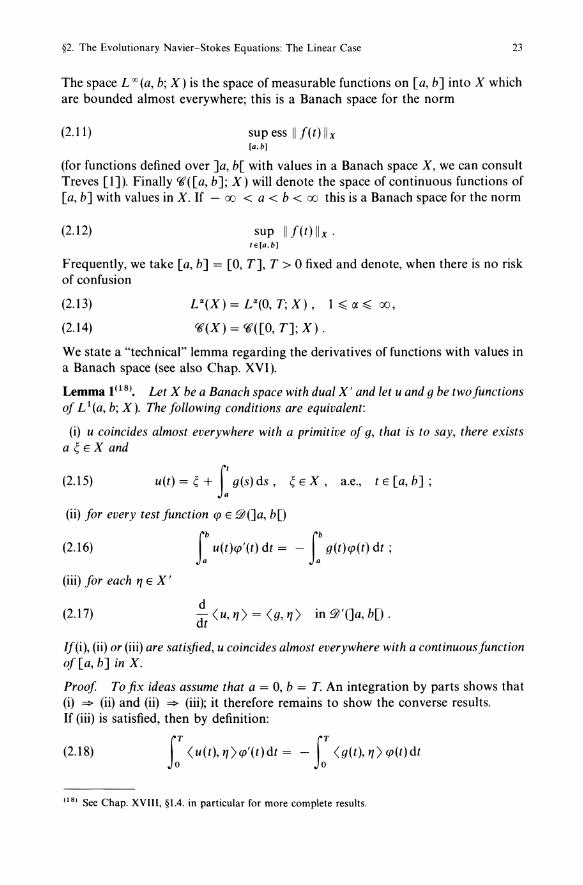
The space L W(a, b; X) is the space of measurable functions on [a, b] into X which are bounded almost everywhere; this is a Banach space for the norm

(2.11 ) sup ess II f(t) Ilx [a.bl

(for functions defined over ]a, b[ with values in a Banach space X, we can consult Treves [1]). Finally <6'([a, b]; X) will denote the space of continuous functions of [a, b] with values in X. If - 00 < a ° fixed and denote, when there is no risk of confusion

(2.13)

(2.14)

L"(X)=U(O,T;X), 1~C(~ 00,

<6'(X) = <6'( [0, T]; X) .

We state a "technical" lemma regarding the derivatives of functions with values in a Banach space (see also Chap. XVI).

Lemma 1(18). Let X be a Banach space with dual X' and let u and g be two functions of L l(a, b; X). The following conditions are equivalent:

(i) u coincides almost everywhere with a primitive of g, that is to say, there exists a ~ E X and

(2.15) u(t)=~+ Lg(S)dS, ~EX, a.e., tE[a,b];

(ii) for every test function qJ E £&(]a, bD

(2.16) r U(t)qJ'(t) dt = - r g(t)qJ(t) dt ;

(iii) for each I] E X I

(2.17) d dt < u, 1]) = <g, 1]) in £&I(]a, bD .

If(i), (ii) or (iii) are satisfied, u coincides almost everywhere with a continuous function of [a, b] in X.

Proof To fix ideas assume that a = 0, b = T. An integration by parts shows that (i) => (ii) and (ii) => (iii); it therefore remains to show the converse results. If (iii) is satisfied, then by definition:

(2.18) f: <u(t),I])qJ'(t)dt= - f: <g(t),I])qJ(t)dt

(18) See Chap. XVIII, §1.4. in particular for more complete results.


for all (i). We can always assume that 9 = O. Indeed, setting v = u - Uo with uo(t)

= L g(s) ds, it is clear that Uo is absolutely continuous and satisfies u~ = g; then

the substitution of u = v + Uo in (2.16) allows us to obtain

(2.19) f: v(t)<p'(t)dt = 0, V0 be a function of ~(] 0, T[) such that f: 4>0( T) dt = 1. Every function 4> of

~(]O, T[) can be written:

(2.20) o(t))dt = 0, the primitive of 4> - A4>o which is null at 0 belongs

to ~(JO, T[) and IjJ is precisely this function). From (2.19) and (2.20).

(2.21) f: (v(t) - O<p(t)dt = 0, V w = 0 a.e.

Result (2.22) is well-known: it is obtained by regularisation. Let w be the function equal to w on [0, TJ and to 0 outside this interval and let Pe be an even regularising function. For 8 small enough Pe * 4> belongs to ~(]O, T[) for every function 4> of ~(]O, T[) and further:

f: w(t)(Pe*<p)(t)dt = f:: w(t)(Pe*<p)(t)dt

= f:: (Pe*W)(t)<p(t)dt.

(19) This implies the stated continuity of the function u over [a, b].


Therefore for fixed I] > 0 and e small enough, P. * W = 0 in the interval [I], T - 1]]. When e --+ 0, P. * w converges to w in L 1 ( - 00, + 00; X) and w = 0 on [I], T - 1]]; since I] is arbitrary, w = 0 on [0, T]. 0

2. Existence and Uniqueness Theorem

2.1. Weak Formulation of the Problem

Let Q be an open bounded set of fRn with boundary aQ and let Q be the cylinder Q x ]0, T[. We look for a vector function u = (Ul, ... , un) representing the velocity of the fluid and a function p representing the pressure, defined in Q and satisfying the following equations, boundary conditions and initial conditions:

(2.23)

(2.24)

(2.25)

(2.26)

au at - vLlu + gradp =f in Q = Qx]O, T[,

div u = 0 in Q ,

u = 0 on aQ x ]0, T] ,

u(x, 0) = uo(x) in Q ;

the vector-valued function u is defined in Q and Uo is defined in Q. In order to obtain an existence and uniqueness theorem we must produce a weak formulation of problem (2.23H2.26). Let (u, p) be a classical solution, for example u E (<6' 2 (Q))n and p E <6' 1 (Q), of (2.23H2.26). Let v be a function of 1/"; writing the scalar product of (2.23) with v and integrating by parts, we obtain(20):

(2.27) ( ~~, v) + v((u, v)) = (f, v) .

By continuity, the preceding equation is valid for every function v of V; further observe that

(~~, v) = :t (u, v) .

It is natural to pose the following definition (Leray [1]):

Definition 1. We call the following problem (2.28H2.32) the weak formulation of problem (2.23H2.26): for given f and Uo,

(2.28)

(2.29)

find u satisfying

(2.30)

(20) See the notation at the beginning of §2.1.

Uo E H.


and

(2.31)

(2.32)

d dt (u, v) + v«u, v» = <f, v) , Vv E V, in E&'(]O, T[),

u(O) = Uo ;

u is called the weak solution of problem (2.23H2.26).

Remark 1. Condition (2.32) does not, in general, have a sense for functions u E L 2(0, T; V); it is justified by Lemma 2 below. 0

Remark 2. The existence and uniqueness of a weak solution is shown in the functional framework defined by (2.28), (2.29), (2.30). It is clear that every classical solution of (2.23H2.26) is a weak solution. The converse, that is to say, every weak solution satisfies (2.23H2.26) in a certain sense, will be proved in §2.3. 0

Lemma 2. Every function satisfying (2.30) and (2.31) is, after modification over a set of measure zero, a continuous function of [0, T] into V'.

Proof Thanks to (2.6) and (2.8), we can write (2.31) in the form:

(2.33) d - < u, v) = < f - v Au, v), V V E V . dt

Since A is linear and continuous from V into V' and u E L 2( V), the function Au belongs to L2(V'); thereforef - vAu E L2(V') and an application of Lemma 1 to (2.33) shows that:

(2.34) u' E L2(0, T; V');

further, u coincides almost everywhere with a continuous function of [0, T] into V'. 0

If (2.28) is satisfied and if u is a weak solution (in particular satisfying (2.30) and (2.31)), then u' E L2(0, T; V') and satisfies (2.33) from the proof of Lemma 1, equation (2.23) is equivalent to:

(2.35) u' + vAu =f.

Conversely, if u satisfies (2.30), (2.34) and (2.35), then u satisfies (2.31). An equivalent formulation of the weak problem of Definition 1 is therefore: for given f and uo, satisfying

(2.28)'

(2.29)'

find u satisfying

(2.36)

(2.37)

(2.38)

UOE H,

U E L 2(0, T; V), U' E L 2(0, T; V') ,

u' + vAu = f in ]0, T[ ,

u(O) = Uo .


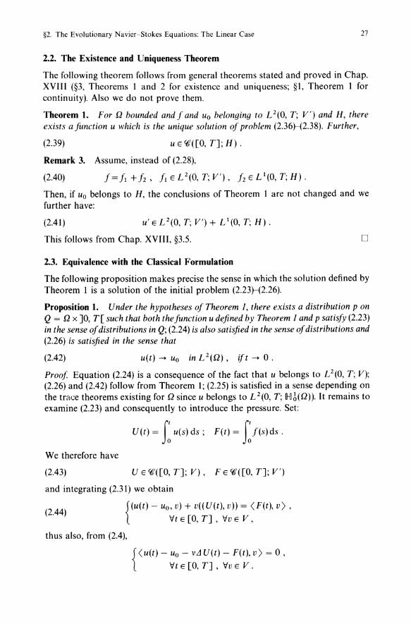
2.2. The Existence and Uniqueness Theorem

The following theorem follows from general theorems stated and proved in Chap. XVIII (§3, Theorems 1 and 2 for existence and uniqueness; §I, Theorem 1 for continuity). Also we do not prove them.

Theorem 1. For Q bounded and f and Uo belonging to L 2(0, T; V') and H, there exists a function u which is the unique solution of problem (2.36H2.38). Further,

(2.39) U E rc([O, T]; H) .

Remark 3. Assume, instead of (2.28),

(2.40) f=f1+f2' f1EL2(0,T;V'), f2EL1(0,T;H).

Then, if Uo belongs to H, the conclusions of Theorem 1 are not changed and we further have:

(2.41 )

This follows from Chap. XVIII, §3.5. D

2.3. Equivalence with the Classical Formulation

The following proposition makes precise the sense in which the solution defined by Theorem 1 is a solution of the initial problem (2.23H2.26).

Proposition 1. Under the hypotheses of Theorem J, there exists a distribution p on Q = Q x ]0, T[ such that both thefunction u defined by Theorem J and p satisfy (2.23) in the sense of distributions in Q; (2.24) is also satisfied in the sense of distributions and (2.26) is satisfied in the sense that

(2.42) u(t) -4 Uo in L2(Q), ift -4 0.

Proof Equation (2.24) is a consequence of the fact that u belongs to L 2(0, T; V); (2.26) and (2.42) follow from Theorem I; (2.25) is satisfied in a sense depending on the trace theorems existing for Q since u belongs to L2(0, T; IHJ6(Q)).1t remains to examine (2.23) and consequently to introduce the pressure. Set:

U(t) = L u(s) ds; F(t) = f~f(S)dS. We therefore have

(2.43) U E rc([O, T]; V), FE rc([O, T]; V')

and integrating (2.31) we obtain

(2.44) {(U(t) - uo, v) + v«U(t), v)) = <F(t), v) ,

Vt E [0, T] , Vv E V,

thus also, from (2.4),

{ < u (t) - Uo - v LI U ( t) - F ( t), v) = ° , Vt E [0, T] , Vv E V.


From Propositions 1 and 2 of §1 there exists, for every t E [0, T], a function P(t) of L 2(Q) such that

(2.45) u(t) - Uo - v,1 U(t) + grad P(t) = F(t) .

But by Proposition 2 of §1 (see also Lemma 6 of §1), the gradient operator is an isomorphism of L 2(Q)/1R into 1Hl- 1 (Q); noting that

grad P = F + v,1 U - u + Uo E C6'([0, T]; 1Hl- 1 (Q)) ,

We deduce

(2.46)

It is thus legitimate to differentiate (2.45) with respect to the variable t, in the sense of Q = Q x ]0, T[; setting p = oP/ot, we obtain precisely (2.23). 0

Remark 4. We cannot in general obtain more information on p = oP/ot than its definition and (2.46). The additional regularity of p depends on additional regularity hypotheses on the data f and uo, as we shall see in Sect. 3 (see however Lions [1]). 0

3. L 2 - Regularity Result

When the data Q (bounded), uo,f are sufficiently regular, we can obtain all of the natural L 2 regularity results on u and p. We content ourselves here with proving two simple results corresponding to a priori estimates obtained formally by "multiplying by u"', then "by Au".

Proposition 2. Let Q be a bounded set of class C6'2. Let f and Uo be such that

(2.47) fEL 2 (0,T;H),

(2.48) Uo E V .

Then the functions u and p defined by Theorem 1 and Proposition 1 satisfy:

(2.49)

(2.50)

(2.51 )

U E L2(0, T; 1Hl2(Q»,

u' E L 2(0, T; H) i.e. u' Ell 2(Q) ,

P E e(O, T; H I(Q)) .

Proof If we obtain a suitable a priori estimate for· the approximate solution Urn (defined by the Faedo-Galerkin method; see Chap. XVIII) we can show (2.50).

rn

In effect, let um(t) = L gim(t)W/21), the solution of: i = 1

(21) We denote, as usual, by WI,' .. , Wi,' .. a basis of V (that is free and total in V).

§2. The Evolutionary Navier-Stokes Equations: The Linear Case

We multiply by gjm(t), 1 ~ j ~ m and add the m equations obtained; we get:

lu~(t)12 + v«um(t), u~(t))) = (f(t), u~(t» or

(2.52) 2Iu~(t)12 + V ~ II um(t) 112 = 2(f(t), u~(t)). dt

29

The integration of (2.52) from ° to T and the Cauchy-Schwarz inequality give us:

or

2 f: I u~(t) 12 dt + v II Um(T) 112 = v II UO m f + 2 f: (f(t), u~(t)) dt

~vlluOmI12+ f: l f(t) 12 dt+ f:lu~(t)12dt,

(2.53) f: lu~(t)12 dt ~ v II UO m 112 + f: I f(t)12 dt .

The elements Wj can be chosen in Vand we can define UOrn as the projection in Vof Uo onto the space generated by Wh ... , Wm such that

(2.54) UO m --+ Uo strongly in V as m --+ 00

and

(2.55)

Under these conditions (2.53) shows us that u~ is bounded independently of m in L 2 (0, T; H), which proves (2.50). We then apply Theorem 10 of §1 in the case IX = 2 to equations (2.23H2.25). This regularity theorem for the stationary case allows us to conclude that u(t) E 1J-11 2 (Q) and p(t) E HI (Q), for almost all t in the interval [0, T] since

1- vL1u(t) + grad p(t) = f(t) - u'(t) E L 2(0, T; 1I..2(Q» ,

(2.60) div u(t) = 0 in Q,

u(t) = ° on 8Q .

From the inequality (1.72) of Theorem 10 of §1, the mapping

f(t) - u'(t) --+ {u(t), p(t)}

is linear and continuous from II.. 2(Q) into 1J-11 2 (Q) x Hl(Q); asf(t) - u'(t) belongs to L2(0, T; II.. 2(Q)), (2.49) and (2.51) are clearly satisfied. D The preceding result can be improved by choosing, for the Galerkin basis, the "special" basis composed of eigenfunctions of the Stokes problem (see §1.2.6). Now here is a very simple lemma.

Lemma 3. Let Q be an open bounded set of [Rn of class ((j 2. Then I Au 1(22) is a norm in V n 1H12(Q) which is equivalent to the norm induced by 1H12(Q).

(22) Recall that A is defined by (2.8).


Proof For u in V andfin IL 2(Q), the problem vAu = fis equivalent to

(2.61) v«u, v» = (f,v) , VVEV.

Theorem 10 of §1 gives:

Ilulll1l'(Q):( Colfl = vColAul·

The inverse inequality is easy. 0

Proposition 3. Let Q be an open bounded set of IR" of class C(} 2. Let f and Uo be such that:

(2.62)

(2.63) UOE H.

Then the function u defined by Theorem 1 satisfies:

(2.64)

(2.65)

In the case where:

(2.66)

jtu E L 00(0, T; V) n L 2(0, T; 1HJ 2(Q»

jtu' E L2(0, T;H).

Uo E V,

then the solution function u satisfies

(2.67)

(2.68)

uELOCJ(O, T; V) n L2(0, T;1HJ 2(Q»

U'Ee(O, T;H).

Proof We proceed as in the proof of Proposition 2, but by using for the sequence of elements the elements WI, ... , W m • ..• (the Galerkin basis) the sequence of eigenfunctions of the Stokes problem introduced in §1.2.6. This allows us to "multiply by Aum " and to obtain supplementary a priori estimates for Um (with Um = Lgim(t)wd. If Uo E V we can define Uo m satisfying (2.54) and (2.55). Substitute Um for u and Wj for v, 1 :( j :( m, in (2.27) then multiply by Aj' the eigenvalue associated with the eigenfunction Wj for 1 :( j :( m. Thanks to relation (1.56) and to (2.8), it becomes

«u:n, Wj» + v(Aum, AWj) = (f AWj) .

We multiply this relation by gjm(t) and sum for j = 1, ... , m and obtain:

1 d (2.69) "2 dt II um(t) 112 + vIAum (t)1 2 = (f(t), Aum(t».

It follows easily that:

d 1 (2.70) -d II Um(t)ll2 + v I Aum(tW :( -If(t) 12 .

t v

In particular,

§3. Additional Results and Review 31

and consequently thanks to the choice of UO m :

(2.71) o~ t~ T.

Finally, by (2.70), we obtain:

fT 1 fT Ilum(T)11 2 +v IAum(t)12dt~ IluoI12+- If(t)1 2dt. o v 0

(2.72)

The estimate (2.71) assures us that Um is bounded independently of m in L 00

(0, T; V). Estimate (2.72) and Lemma 3 assure us that Um is bounded independently of min L2(0, T; 1HJ 2(Q)). A standard passage to the limit leads to the conclusion that (2.67) is satisfied. We remark that u' = f - vAu, from which we deduce (2.68). If Uo E H, we multiply (2.70) by t and obtain:

d t -d (tllum I1 2) + vtIAum(t)1 2 ~ -If(t)12 + II um(t) 112 .

t v (2.73)

Therefore jtum is bounded, independently of m, in

Loo(O, T; V) n L2(0, T; 1HJ2(Q));

(2.64) is satisfied. We remark that jtu' = jt(f - vAu); (2.65) then follows. 0

§3. Additional Results and Review

1. The Variational Approach

The study of the linearised Navier-Stokes equations (stationary and evolutionary) confirms the positive qualities of the variational approach. Starting from wellchosen functional spaces, we obtain existence and uniqueness results simply and constructively. The choice offunction spaces is therefore essential and we have seen that their study (§ 1.1. and §2.l), which is the most difficult part of the work here, is very technical. However, variational methods are insufficient when we want to obtain regularity results a priori or are interested in the existence of regular solutions. Some partial results can be obtained in the case of L 2 regularity, but we have to resort to other methods for the study of L 0 regularity.

2. The Functional Approach

The theory of operators allows us to interpret usefully certain important results of §1 (or of §2). For example, Lemma 6 of §1, says that the gradient operator is an isomorphism of L2(Q)/~ into 1HJ- 1(Q) whose image is closed.


The image therefore coincides with the orthogonal set of the kernel of the formal adjoint operator which is the divergence. Theorem 6 of §1 says that the kernel is

{u E IHlMQ), div u = O} .

Proposition 1, which follows, makes precise the properties of the operator A associated with the Stokes problem: it therefore completes the results of §2 and prepares, on the other hand, for the study of the nonlinear Navier-Stokes equations. Let P be the orthogonal projection of IL 2(Q) over H (see §1.1 for the notation). We know that the space V is a Hilbert space for the scalar product

n

«u, v)) = L (DiU, Di V )

when the open set Q is bounded (which we assume). The following inclusions are therefore satisfied:

V c H = H' c V'.

Let A be the canonical isomorphism of V (equipped with the norm II II) into V' introduced by (2.8) in §2.1. The operator A can be considered as an unbounded operator in H, therefore with the following properties.

Proposition 1. Let Q be a bounded set of [R2 or [R3 whose boundary is of class C(j2. Then: (i) the domain of A in H is DH(A) = 1Hl2(Q) n V, which is dense in V, and IAul is

a norm over DH(A) which is equivalent to the norm induced by 1Hl2(Q):

(3.1) Clllul2~IAul ~ClluI2' uEDH(A)(23);

(ii) Au = - P Llu, Vu E DH(A) and A is the Friedrichs extension of - Lll v

(iii) iff Ell 2(Q) or iff E H, the two assertions vAu = f and there exists pEL 2(Q) such that (u, p) is the solution of the homogeneous Stokes problem, are equivalent; (iv) A is a positive, self-adjoint operator with compact inverse. (v) There exists an orthonormal basis of H, {wm },~'= 1 and positive real numbers {Am} ~ = 1 such that

(3.2)

and further there exists a constant qQ) such that:

(3.3) Am ~ C(Q)m2/n (n is the space dimension) .

It follows from (1.42) and (2.8) that the operator A is related to the operator A seen in § 1.2.6 by:

1 therefore A IH = - A-I.

V

(23) With the notation I u 12 = II U 111121<2)' and with C I = constant.

§3. Additional Results and Review 33

Proof Point (i) follows from Cattabriga [1], Solonnikov [1] or VorovichYudovich [1] (see Theorem 11 of §1). Point (ii) follows from Fujita-Kato [1]. By modifying p we can always assume that f E H, i.e. Pf = f point ii) is then immediate from what has gone before. We verify easily that A is positive self-adjoint and the compactness of A -1 follows from the compactness of the injection of IH16(Q) into IL 2(Q is bounded). The first property of v) follows from iv); so (3.3) is a particular case of Metivier [1]. D

Remark 1. If Q is of class Ifjk a repeated application of Theorem 11 of §1 shows that:

In particular, if Q is of class Ifj 00

Wm E (lfjOO(Q))", Pm E IfjOO(Q) , m ~ 1 .

3. The Problem of L" Regularity for the Evolutionary Navier-Stokes Equations: The Linearised Case

D

The problem of L" regularity has already been approached for the stationary case in §1.3.

The evolutionary case presents the same difficulties. It assumes the explicit construction of the solution of the Cauchy problem in [R3 (in the case n = 2, we can proceed as in §1.3.2):

u' - vLlu + gradp =f in [R3 x]O, T[,

(3.4) div u = ° in [R3 + ]0, T[

u(x, 0) = ° in [R3 .

We shall be content to state an example of the result and refer to Ladyzenskaya [1] and particularly to Solonnikov [1], [2], [3] for the statement of compatibility conditions and for proofs. Let Q = Q x ]0, T[; we denote by W~·l( Q) the space of functions whose derivatives of order ~ k with respect to x are in L" and the derivatives of order ~ I with respect to t are in L ", and 'MY~.I( Q) its vector-valued version(24). We consider the problem:

(3.5)

au at - vLlu + grad p = f in Q

div u = ° in Q u = ¢ over aQ x ]0, T[ ,

u It = 0 = Uo in Q .

(24) With similar notation when we replace Q by oQ x ]0, T[.


Theorem 1. Let Q be an open bounded set of ~3 of class C(j 2r+ 2(r EN). We assume that (for IY. > 1 and IY. =1= 3/2):

(a)

(3.6)

2

(3.7) Uo E W;k+ 2 -a(Q) !l H 1 I

(3.8) qJEW;k+2- a,k+I-2a(oQx(O,T)) and <p.v=O overoQx]O,T[;

(b) necessary compatibility conditions are satisfied up to a sufficient order (we shall not make this explicit). Then problem (3.5) has a unique solution (u, p) such that:

(3.9)

Further the following estimate is satisfied:

3

I {II Ui II Wa"+2k+ I(Q) + II DiP II Wa"·k(Q)} i= I

3

(3.1 0) ~ C I {II}; II W;k.k(Q) + II UOi II W,H+ 2-~(Q) i= 1

(We again denote u = (Uj, ... , un), f = (fl, ... fn), <p = <PI, ... , <Pn)).

Documents

Mathematical Analysis and Numerical Methods for Science and Technology || The Linearised Navier-Stokes Equations