Embed Size (px)
Citation preview
Chapter XXI. Transport
§ 1. Introduction. Presentation of Physical Problems
The problems of neutron transport have been presented in Chap. lA, §5. We recall the essentials below.
1. Evolution Problems in Neutron Transport
1.1. The Integro-differential Transport Equation (Ref. Bussac~Reuss [1], Benoist [1], Duderstadt~Martin [1], Case et al. [1], Davison~Sykes [1], Weinberg~Wigner [1] ).
This equation describes the evolution of a population of neutrons in a domain X of 1R3 occupied by a medium which interacts with the neutrons. 1) A neutron is described by
~ its position x E X C 1R3; ~ the direction of its velocity v(l): w in SZ (the unit sphere of [R3)
~ its kinetic energy E = ml viz /2, (m is the mass of the neutron and v its velocity vector), with E in [iX, fJl We set Q E = X X SZ X [iX, fJl 2) The interaction between the neutrons and the atomic nuclei of the medium, and therefore the production of neutrons in the collisions, are assumed to be described by functions denoted EAx, E), Ls(X, w' -> w, E' -> E), L f(x, E') (called respectively the effective total cross section, the diffusion or transfer cross section and the fission cross section), K(E) and v(x, E'); L, (t for total) takes into account all the categories of collisions of neutrons with kinetic energy E at x; Ls (s for 'scattering' = diffusion) takes into account the neutrons with kinetic energy E'and direction w', which by collision at x, take kinetic energy E and direction w(Z); L f (f for fission) takes into account the neutrons with kinetic energy E' which induce fission at x; K(E) is the spectrum of neutrons emitted by the fission, normalised so that J K(E)dE = 1; v(x, E') is the average number of neutrons emitted from a fission at x due to a neutron with kinetic energy E'.
(1) Each neutron is assumed to travel in a straight line between collisions with the atomic nuclei of the medium; the only changes of direction are due to these collisions. (2) The medium is assumed isotropic, L, only depends on the directions wand w' through the scalar product w. w', and L, and LJ are independent of wand w' (from which we have the notation L,(X, E), LJ(X, E) adopted above). In the case where the medium is anisotropic, this will no longer necessarily be true. In the case of an isotropic medium, where further L, is independent of w' . w, the collision is called isotropic.
R. Dautray et al., Mathematical Analysis and Numerical Methods for Science and Technology
© Springer-Verlag Berlin Heidelberg 2000
2\0 Chapter XXI. Transport
The functions Lt , L., L f' K and v are assumed given, positive and bounded. There exists a source of neutrons described by a given scalar function S(x, w, E, t). 4) The population of neutrons is described by a scalar function u(x, w, E, t), which is the angular density of the number of neutrons at (x, w, E) E QE at the moment t. We also define the density of angular flux ct>(x, w, E, t) by
ct>(x, w, E, t) ~ I vi u(x, w, E, t) .
Remark 1. We define the total density %(x, E, t) and the total flux cP(x, E, t) of the neutrons of energy E at a point x at the moment t, from u and ct> via the formulae
11) %(x, E, t) ~ t ii(x, w, E,t) dw ,
II) cP(x, E, t) = f ct>(x, w, E, t) dw S2
o
The density of angular flux ct> satisfies the (evolution) transport equation
1 act> f;I at (x, E, w, t) + w. VxcI>(x, w, E, t) + Lt(X, E) ct>(x, w, E, t)
(1.1) - fP dE' f Ls(X, w' -+ W, E' -+ E)ct>(x, w', E', t) dw' a S2
-4K(E) fP v(x, E)L f(x, E') dE' f ct>(x, w', E', t) dw' = S(x, w, E, t)(3) n a S2
We also use the variables (x, v), where the velocity vector v of the neutron belongs to the domain V c [R3 and denote(4)
def m _ u(x, v, t) = - u(x, w, E, t)
Ivl L(X, v) ~ IvILt(x,E)(5)
(1.2) f( ') ~ ~ ['<"' ( , E' E) K(E)v(x, E')Lf(x, E') J x, v, v - m Ivl '<'s x, W -+ W, -+ + 4n '
( ) ~ m S( E )(6) q X, v, t - -I x, w, ,t vi
3
(3) With the notation w. VA) = L w,ocp/ox,. In what follows V denotes the gradient taken with j= 1
respect to the variable X(XEX c [];l3).
(4) As in the majority of publications (5) The medium being isotropic, L only depends on v through lvi, and J only depends on v and v' through lvi, Iv'l and v'. v. However for more generality, this hypothesis of an isotropic medium will not necessarily be made in this chapter. (6) S(x, W, E, t) denoting an angular density of (number of) neutrons in (x, w, E) E QE at the moment t, per unit time (due to a source of neutrons in the medium considered) is a priori a positive quantity; it is the same for q(v, x, t).
§1. Introduction. Presentation of Physical Problems 211
Taking account of (1.1), the unknown function u(x, v, t) must satisfy the (evolution) transport equation
(1.3)
au ot (x, v, t) + v. Vu(x, v, t) + I'(x, v)u(x, v, t)
- Iv f(x, v', v)u(x, v', t) dv' = q(x, v, t)(7)
with (x, v) E Q ~f X X V and t > 0 .
The unknown functions ¢ and u must be positive. Further, the total number N of neutrons in the bounded domain X must be finite at each moment t(8), so that
N(t) = I u(x, v, t) dx dv = I u(x, w, E, t) dx dw dE JQ JQ, (1.4)
= t. V(~) ¢(x, w, E, t) dx dw dE < 00 (9) .
The evolution problem for the transport equation, called the Cauchy problem, consists of determining the unknown function ¢(x, w, E, t) satisfying (1.1) with the initial condition
(1.5) ¢(x, w, E, 0) = ¢o(x, w, E) ,
¢o being the angular flux at the moment t = 0 and with some boundary conditions on the boundary ax of the domain X (respectively: determine u(x, v, t) satisfying (1.3) with the initial condition
( 1.5)' u(x, v, 0) = uo(x, v) ,
uo(x, v) being the neutron density at the moment t = 0 and with suitable boundary conditions).
(7) It is useful in certain applications to set f = Lj(p) with
j(P)(x, v', v) = L(p)(X, v')g(P)(v', v)c(p)(x, v')
where c(p) (x, v') is the average number of neutrons emitted in a collision at x of speed v', g(P)(v', v) the probability that an incident neutron of speed v' causes, in a collision, the emission of neutrons of speed v, and Lp(X, v') the macroscopic cross section (corresponding to the process (p)) of a neutron of speed v' at the point x with suitable normalisation. The processes already mentioned are not the only ones which can occur in applications [e.g. (n, 2n), (n, 3n), etc ... ]. (8) We obviously assume that q is a source of a finite total number of neutrons at each moment t, so that q(. , . , t) ELI (X x V). (9) With the notation
(2E v(E) = Ivl = V -;;; .
212 Chapter XXI. Transport
Remark 2. The multigroup equations of transport. In applications we ordinarily treat the influence of the parameter E on the equation (1.1) by dividing the interval of variation [IX, P] of E into subintervals which we call energy groups:
[1X,1X1][1X1,1X2]'" [lXg,lXg+l]'" [lXm-l,P]·
Equation (1.1) is then replaced by a system of equations determining the average flux in each energy group. The cross sections and the other data depending on E are replaced by the average cross sections for of the energy groups considered, called muItigroups. To calculate the muItigroup cross sections is one of the essential stages in the analysis of a reactor (see Bussac-Reuss [1]). The same considerations also apply to equation (1.3). We then write the system of m multigroup equations
(1.6) D
with g = 1,2, ... , m
1.2. Boundary Conditions.
1.2.1. Neutron Problem in a Convex Domain X c [R3, whose Exterior [R3\X is Occupied by a Vacuum (or in an arbitrary domain X surrounded by a medium which totally absorbs neutrons). We assume here that every neutron which arrives at a point of ax from the interior of X disappears and that neutrons never arrive from the exterior: the neutron flux entering X at each point of ax is zero, that is to say
(1.7) {<P(X, ill, E, t) = 0 '<It? 0 and a.e. (x, ill, E) E ax x S2 x [IX, P] such that ill' v(x) < 0 .
(where v(x) denotes the outward normal to ax at X). We shall call (1.7) the absorption boundary condition.
1.2.2. The Case of a Source Placed at the Boundary ax. Here the angular flux 'entering' X at the boundary ax is known (and nonzero), so that
(1.8) {<P (x, ill, E, t) = go(x, ill, E, t) '<It? 0 and a.e. (x, ill, E) E ax x S2 x [IX, P] such that ill. v(x) < 0 .
1.2.3. The Case of Symmetric Boundary Conditions. When the domain X and the data which are considered have groups of symmetries the solution of the transport equation which interests us will have the same symmetries. We restrict ourselves to treating the 'elementary motif'OO) and to applying the boundary conditions which we deduce to those of the original problem (see Bussac-Reuss [1], fourth part).
(10) This 'elementary motif', completed by the group of symmetries of the problem, gives the entire domain Q.
§l. Introduction. Presentation of Physical Problems 213
1.3. The Integral Equation of Transport
We shall show that the Cauchy transport problem formed from the integrodifferential transport equation which we take in the form (1.3) (with for example X = 1R3 ) with the initial condition,
(1.9) u(x, v, 0) = uo(x, v) a.e. (x, v)
is equivalent to the integral equation
(1.1 0)
u(x, v, t) = uo(x - vt, v) exp ( - f~ ..r(x - vs, v) ds )
+ f~{Q(X'-V(t-S),u,s)exp( - f~-s..r(x-Ur'U)dr)}ds,
with the notation
(1.11) Q(x, v, s) = Iv f(x, v', u)u(x, u', s) dv' + q(x, v, s) .
In the case where the domain X is different from 1R3 , the boundary conditions (1.7) lead to an analogous formula (see §2). The equation (1.10), called the integro-differential transport equation, is very useful in numerous applications: - it is the basis of numerical solution methods called the methods of collision probability (and some derived methods) which are largely used in codes to analyse cells and assemblies of nuclear reactors (see Hoffmann et al. [1]); - the integral transport equation allows us to study with simplicity certain properties of the transport operator T occurring in (1.3), an operator which will be made more precise in (1.13), (1.14).
2. Stationary Problems
By the expression: stationary solutions, we usually denote in neutron physics the solutions of the transport equations (1.1) or (1.3) which are independent of time. The phenomenon described by these functions cp, u independent of time corresponds to a migration of neutrons at constant rate. The stochastic processes which describe these migrations, are themselves stationary in the probabilistic sense of the word.
2.1. Stationary Problems for the Neutron Transport Equation
We shall consider equation (1.3)(1 \) with q independent of t, and the boundary condition of type (1.7) or (1.8) (but go only depends on t). The stationary transport
(11) It will also be possible to consider (1.1)
214 Chapter XXI. Transport
problem is written: find u(x, v) satisfying (for q and g given):
( 1.12) {(i) - Tu(x, v) = q(x, v) a.e. (x, v) E X X V ,
(ii) u(x, v) = g(x, v) a.e. (x, v) E ax x V , with
(x, v) E ax x V satisfying v . v(x) < 0 where v(x) is the outward normal to ax at x. The operator T, called the transport operator, occurring in (1.12) is such that:
(1.13) Tu(x, v) = - v. Vu(x, v) - I'(x, v) u(x, v) + Iv f(x, v', v) u(x, v') dv' .
It is naturally defined in the space L 1 (X X V) of integrable functions in (x, v) and its domain D( T) is (see §2)
(1.14) { D(T)= {u:uEL1(XX V), TUEL1(XX V)
and [u(x, v) = 0 a.e. (x, v) E ax x V and v. v(x) < O]}
In the muItigroup case, this operator, denoted T m is given by
( 1.15) D(Tm) = {{ug}, g = 1 to m, ugEL 1(X x V), Tm{Ug}EL1(X x v)m ,
ug(x, v) = 0 a.e. (x, V)EcJX x V and V' v(x) < O}
The study of the properties of the operator T allows the solution of evolution problems and of stationary transport problems, and the approximation 'of transport' by 'diffusion'. Integral formulation (see Bussac-Reuss [1], Benoist [1]). The analysis of the transport of neutrons in heterogeneous combustible nuclear reactor assemblies are almost always carried out in a stationary regime; they are often based on the integral form of the stationary transport equation which we write, for X = [R3:
(1.16) u(x, v) = L"" dsQo(x -sv, v)exp - [f: I'(x -tv, v)dt J where Qo(x, v) = Iv f(x, v', v)u(x, v') dv' + q(x, v).
The multigroup formulation of this equation is
(1.17) ug(x, w) = fow
ds Qg(x - sw, w) exp [ - f: P(x - tw, w) dt J with g = 1 to m, and
Qg(x,w) = 9'~1 Is2P,~g(X'W"W)ug(X'W')dW' + qg(x).
§2. Existence and Uniqueness of Solutions of the Transport Equation 215
3. Principal Notation
We shall set:
(1.18) f ~fax x V, ro ~f {(X,V)Er, v. v(X) = O}
[r+ ~ {(X,V)Er,V.V(x»O} , L={(X,V)Er,V.V(x)<O}
where v denotes the outward normal to ax at x. In this chapter we shall use the form (1.3) of the transport equation, with the initial conditions and with the boundary conditions (homogeneous or nonhomogeneous):
(1.19)
(1.20)
u(x,v,t)=o '<It >0, a.e.(x,v)Er_
u(x,v,t) = go(x,v, t) , '<It >0, a.e.(x,v)EL.
§2. Existence and Uniqueness of Solutions of the Transport Equation
1. Introduction
We study the equation (1.3) with null source (q = 0) and consider, for the sake of simplicity, the case of absorbing boundary conditions, that is to say (1.19). We therefore consider the following problem: find a function(12) u = u(x, v, t) satisfying
i) ~~+v.VU+LU=KU xEXclRn , vEVclRn , t>O (13)
(2.1) ii) ul r_ = 0, t ~ 0, L defined by (1.18)
iii) u(x, v, 0) = uo(x, v), Uo given,
where L is a given positive function(14) of x and v and where the given operator K is defined by
(2.2) (Ku)(x, v, t) = Iv f(x, Vi, v)u(x, Vi, t) dJl(v' ) .
In this expression, f is a given function, positive since it models a transfer of a density of numbers of neutrons from one speed to another, the two densities being positive(15).
(12) The value u(x, v, t) models the density of neutrons at the moment t, at (x, v) must be positive, as must the initial condition Uo (x, v) for (x, v) E X X V, in (2.1)iii). Equation (2.1 i) is written in such a way that only positive terms appear (apart from the derivatives of u). (13) Recall the V = Vx denotes the gradient at x. (14) The positivity hypothesis on L is not often necessary for the stated theorems, but it is essential that we assume L is bounded. (15) f(x, v', v) is directly linked to the probability density for the neutrons at x to change from speed v' to v.
216 Chapter XXI. Transport
We assume that 11 is a positive Radon measure on [Rn with 11( {O} ) = 0, and V is the support of 11; thus V is a closed set of [Rn, for example a ball, a domain ex ~ I v I < f3 or a finite union of spheres (which we shall meet in numerous applications), and likewise, a union of tori and spheres(!6). The existence and uniqueness theorems and the theorems of the positivity of the solutions of evolution problems or of the stationary problems of this §2 are treated in a very general framework and are valid for any space V below. On the contrary, the spectral theory of §3 is valid here, uniquely for V being a ball, a domain ex ~ I vi < f3 or a union of spheres (continuous or multigroup formulation, see §1). A mixture ofthese two situations leads to a more complicated spectrum (see Larsen [2]). In the approximation of the diffusion of §5, we shall see that the symmetries of the space V play an essential role. In applicationsn = 1,2 or 3. We shall keep [Rn however in order not to multiply the proofs. To solve problem (2.1), we shall use the theory of semigroups developed in Chap. XVII. For this, we must firstly choose a functional framework: we look for the solution u which we also write u(t) == u(x, v, t) as a function of time t with values in the space U(X x V)(p E [1, + 00 [) defined as the space of measurable functions f (for the product measure dx dl1) and such that
(2.3) Ilfllu(xxv)==(txv If(X,V)IPdXdl1 )!IP < +00.
The choice p = 1 is natural from the physical point of view, since u is a positive function(! 7) and that
f u(x, v, t) dx dl1(v) xxv
represents the total number of particles at the moment t, which is finite. The case p = 00 must be studied separately. For example, there is already a difficulty with the operator d/dx as the infinitesimal generator which generates the group of translations ¢ --+ G(t) ¢ = ¢( . - t); G(t), t > 0, is a family of operators in L 00 ([R), but is not strongly continuous (of class ~o): in effect, if t --+ 0, II G(t)¢ - ¢ II 00
may not tend to ° (see Chap. XVIIA). Although the quantity
f U2 (x, v, t) dx dl1(v) xxv
does not have a physical interpretation, we shall however often work in §3, for spectral problems, in the space L 2(X x V) which is a Hilbert space, and allows us to use the Fourier transform conveniently.
(16) We always assume (implicitly) in what fo1\ows that the given data 1: and f are measurable for the product measures dx dJl and dx dJl(v)dJl(V'). (17) We may equa1\y look for a solution in a space of suitable measures; the choice u(t) E U(X x V) implicitly eliminates some possible concentrations of particles at points. The solution of (2.1) for UoEU(X x V) (and for a suitable source q)), gives U(t)EU(X x V), '1/ > 0, shows particularly that we cannot have a concentration of particles at a point at any moment / > 0 if we do not have a concentration of particles at that point at the moment / = O.
§2. Existence and Uniqueness of Solutions of the Transport Equation 217
Then let A be the unbounded operator in U(X x V) defined by
{(AU)(X, v) = - v. Vu D(A) = rUE U(X X V); AUE U(X x V), ulr_ = O}, pE [1, oo[
Problem (2.1) is equivalent to the problem
(2.1)' f ~~ = Tu
l u(O) = Uo
where T=A-l:+K,
the operator K being defined by (2.2) (K is an integral operator which is bounded in U(X x V) under certain hypotheses which we shall make on the kernel f). To solve problem (2.1)" we shall determine the semigroup generated by the operator T. We shall see that this is a semigroup of class ceO in U(X x V). We shall firstly study the semigroup generated by the operator A called the advection operator. Definition of the spaces £tJ([Rn x V) and £tJ'([Rn x V) (or £tJ(X x V) and £tJ'(X x V), X open c [Rn. Since the set V is a closed subset of [Rn, it is necessary to make more precise the notion of a distribution over [Rn x V, and the duality £tJ([Rn x V), £tJ' ([Rn x V) used with the pivot space L 2 ([Rn X V, dx d,u) where ,u is not necessarily the Lebesgue measure. First of all the spaces L 2 ([Rn x [Rn, dx d,u) and L 2([Rn X V, dx d,u) are identical since V is the support of ,u. Let J be the continuous mapping which transforms every function cp E £tJ(~n x [RII) into its equivalence class ¢ (for the measure dxd,u) in U([Rn x V, dx d,u); J is not injective, its kernel is: ker J = {cp E £tJ([Rn x [Rn), cp I~" x v = O}. We denote by:
£tJ ([Rn x V) = {cp I ~" + v, cp E £tJ ([Rn x [Rn)} .
The space £tJ([Rn x V) is identical to the quotient space £tJ([Rn x [Rn)/ker J; besides £tJ ([Rn x V) is dense in U ([Rn x V, dx d,u). Note now that every element U E L 2([Rn X V, dx d,u) may be identified with a distri-
bution ii over [Rn x [Rn: cP E £tJ([Rn x [Rn) --+ r ucp dx d,u. JlRllxlRlI
We denote by: £tJ'([Rnx V) the closure of L2([Rnx V,dxd,u) in £tJ'([Rnx[Rn). The space £tJ'([Rn x V) is identified with the dual of the space £tJ([Rn x V), the duality being the extension of the scalar product in L 2 ([Rn x [Rn, dx d,u). In effect, the set of continuous linear forms over £tJ([Rn x V) (equipped with the quotient topology of £tJ([Rn x [Rn)/ker J) is identified with the space:
(kerJ)O = {UE£tJ'([Rnx[Rn),<u,cp> = 0 VcpEkerJ}.
In an obvious way £tJ'([Rn x V) c (kerJ)o. Suppose that there exists uoE(kerJ)O, with Uo ¢ £tJ' ([Rn x V); consequently from the Hahn-Banach Theorem, there exists
cp E £tJ(~n x [Rn) such that < Uo, cp> = 1, < w, cp> = 0 Vw E £tJ'([Rn x V) ,
218 Chapter XXI. Transport
therefore
r uq> dx dJi = ° \fu E L Z(lRn x V, dx dJi), from which q>IR' x v = 0, q> E ker J , JR'XR'
which contradicts <uo, ¢) = 1, from which we have the equality .@'(lRnx V) = (ker J)o. We remark that the space .@'(lRn x V) is a priori contained in the space denoted .@~" x v(lRn x IRn) of distributions over IRn x IRn with support contained in IRn x V. If V is the closure of an open set (9 of IRn( 18), then .@'(lRn x V) = .@~, x v(lRn x IRn).
Proof Suppose that there exists Uo E .@~, x v( IRn x IRn), Uo ¢.@' (IRn x V). Then there will exist q> E.@ (IRn x IRn) such that < Uo, q> ) = 1, < W, q» = ° \fw E.@' (IRn x V); therefore q> I R' x V = ° from which q> I R' x l'J = 0, supp q> c IRn x IRn\ IRn x (9; but then from the properties of derivatives (see Chap. V, § 1),
suppDaq> c IRn x IRn\lRn x (9 for every derivative Da ,
therefore Daq>IR'xl'J = 0, from which by continuity Daq>IR'x v = 0. Thus ¢ and all its derivatives are zero over the support of uo, therefore < Uo, ¢) = o! D
We have therefore given a characterisation of the space .@'(lRn x V) if V = @. If Vis a regular surface (a sphere for example), we refer to L. Schwartz [1], p. 101, 102. We shall note that in the general case (Va closed set of IRn), .@'(lRn x V) is also the closure of U(lRn x V, dx dJi) in .@'(lRn x IRn) for every p E [1, + 00 [since '@(lRn x V) is dense in U( IRn x V, dx dJi): therefore .@' (IRn x V) is independent of p. Finally, in the case where IRn is replaced by the open set X c IRn, the definition of the spaces .@(X x V), .@'(X x V) is adapted without difficulty with the properties previously stated.
2. Study of the Advection Operator A = - v . V
2.1. The Case of the Entire Space (X = IRn, V c IRn as in Sect. 1).
Firstly, let v EVe IRn be a given speed. Consider the problem
f ~u + v. Vu = ° X E IRn, t > ° l u;x, v, 0) = ¢(x, v) (where ¢ is given)
whose solution is given by
u(x, v, t) = ¢(x - vt, v) .
(18) Thus V may be a closed ball, or a domain {x E ~., a ,,:; Ixl ,,:; b, with 0,,:; a < b}.
§2. Existence and Uniqueness of Solutions of the Transport Equation 219
Let G(t), t E [R, be the family of operators defined for q> E ~~ ([Rn X V)(19) by
(2.4) (G(t)q> )(x, v) ~ q>(x - vt , v), Vx, v E [Rn x V.
Proposition 1. The family of operators G(t), t E [R, defined by (2.4) is extended into a group of operators of class ~o over U( [Rn x V) for 1 ~ p < + (fJ, with
(2.5) II G(t) q> II U(u;!" x V) = II q> II U(u;!' x V), Vq> E U([Rn X V) .
The irifinitesimal generator of this group is the operator A defined by
(2.6) { Au = -v. Vu D(A) = {UEU([Rnx V); v. VUEU([Rnx V)} .
Finally this group operates in the cone of positive functions of U([Rn x V).
Proof We remark firstly that if q>E~~([Rn X V)
II G(t)q> - q> II U(u;!" x V) = (r I q>(x - vt, v) - q>(x, v)IP dx dll(V) )1!P -+ 0 JIRIIX V
when t -+ O. By the density of ~~([Rn x V) in U([Rn x V) for 1 ~ p < + 00, we deduce that (G(t»rEu;! can be extended into a semigroup of class ~o over U([Rn X V). We likewise establish (2.5). To find the infinitesimal generator of G(t), we remark that
d dt(G(t)¢)lr=o=-v.V¢ in !»'([RnxV), Vq>ED(A).
From which we deduce (2.6). D
Orientation (to treat the case of an open set x C [Rn). We shall now establish a trace theorem. Here, we come up against a difficulty: if U E LP(X x V) and v. Vu E LP( X x V), it is not true in general, that the trace U I r _ of U on r _ satisfies, with the notation dr _ = dydll on r _ (and likewise dr + = dydll on r+) where dy is the measure of the surface ax:
L- (v' v)lulPdL < + 00
(even in the case p = 2). Naturally, it is no better for the trace ul f+ of u on r +. On the other hand if K is a compact set included in r _ (or r +), we shall see that we can define the trace ulK ofu on K in U(K), which is sufficient to give a meaning to the domain D(A) of the advection operator in the case of absorbing boundary conditions. In order to treat the case of reflection type boundary conditions we are led to using more precise trace theorems.
(19) '6'~ (IRn x V) denotes the space of continuous functions, with compact support, in IRn x V.
220 Chapter XXI. Transport
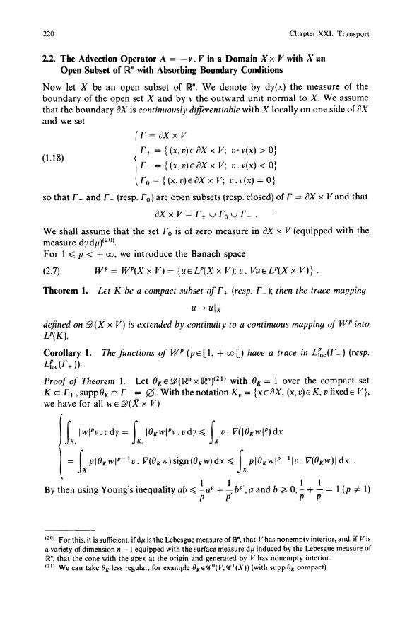
2.2. The Advection Operator A = - v . J7 in a Domain X x V with X an Open Subset of IR" with Absorbing Boundary Conditions
Now let X be an open subset of IR". We denote by dy(x) the measure of the boundary of the open set X and by v the outward unit normal to X. We assume that the boundary ax is continuously differentiable with X locally on one side of ax and we set
(1.18) 1 ~+=~~(:':)EaXX V; v'v(x) >O}
L = {(x, V)EaX x V; v. v(x) < O}
ro= {(X,V)EaXX V; v.v(x)=O}
so that r + and r _ (resp. ro) are open subsets (resp. closed) of r = ax x V and that
ax x V = r + U r 0 u r _ .
We shall assume that the set ro is of zero measure in ax x V (equipped with the measure dydfl)(20). For 1 ~ p < + 00, we introduce the Banach space
(2.7) WP = WP(X x V) = {UEU(X x V); v. VUEU(X x V)} .
Theorem 1. Let K be a compact subset of r + (resp. r _); then the trace mapping
u -+ UIK
defined on £»(X x V) is extended by continuity to a continuous mapping of WP into U(K).
Corollary 1. The functions of WP (p E [1, + 00 [) have a trace in Lfoc(r -) (resp. Lfoc{r +». Proof of Theorem 1. Let OKE£»(IR" x 1R")(21) with OK = 1 over the compact set K c r +, SUPpOK n r _ = 0. With the notation Kv = {XEaX, (x, v)EK, v fixedE V}, we have for all WE £»(X x V)
t, IwIPv. vdy = t, IOKWIPv. vdy ~ Ix v. V(IOKWI P) dx
= Ix plOKWlrlv. V(OKW) sign (OKW) dx ~ Ix pIOKWIP-1I v . V(OKw)1 dx
By then using Young's inequality ab ~ ~ aP + ~ bP', a and b ~ 0, ~ + ~ = 1 (p i= 1) p p' p p
(20) For this, it is sufficient, if dJl is the Lebesgue measure of !R", that Vhas nonempty interior, and, if Vis a variety of dimension n - I equipped with the surface measure dJl induced by the Lebesgue measure of !R", that the cone with the apex at the origin and generated by V has nonempty interior. (21) We can take Ih less regular, for example liKE~O(V,~I(X)) (with suppliK compact).
§2. Existence and Uniqueness of Solutions of the Transport Equation 221
with a = Iv. V(8K w)l, b = 18K wl p - 1 therefore bP' = 18K wI P1(P-l) = 18K w1P, we obtain:
L, IwlPv. v dy ~ Ix 18K wlPdx + (p -1) Ix Iv. V(8K w)IPdx .
With the hypotheses made on 8K , there therefore exists (J(o > 0 constant (independent of v):
L, I wi Pv . v dy ~ (J(o [ Ix [I w I P + I v. Vw I P] dx ] .
By integrating in v, with:
II w II W'(X x VI ~ [Ix x v (I wlP + Iv. VwI P) dx djl JIP ,
we then have:
II wid U(K,v'vdydJl) ~ (J(o II w II W'(Xx V) •
In the case p = 1, we again obtain this inequality with the help of
L, Iwlv. vdy ~ Ix Iv. V(8K w)1 dx ~ (J(o Ix [Iwl + Iv. Vwl] dx.
Now the space !0(X x V) is dense in WP(X x V) (see for example Bardos [1], Lax-Phillips [1], Friedrichs [1]); it follows that the mapping w-> wlr extends by continuity from !0(X x V) to WP(X x V) into U(K, v. v dy djl), or even in U(K,dydjl) since Ijl.vl = jl.v is bounded below in K. From which we have Theorem 1. 0
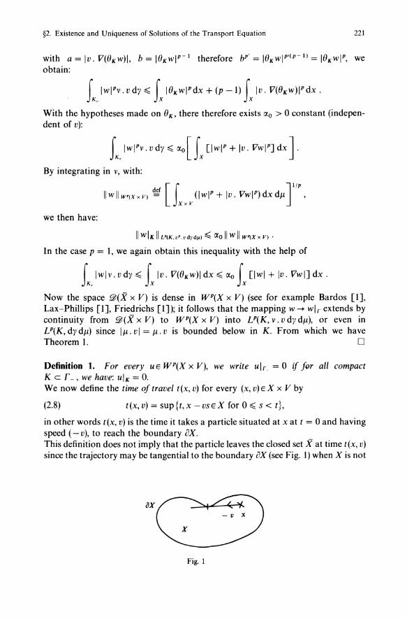
Definition 1. For every UE WP(X x V), we write uk = 0 if fQr all compact K c r _ , we have: U I K = O. We now define the time of travel t(x, v) for every (x, v) E X X V by
(2.8) t(x, v) = sup{t,x -VSEX for 0 ~ S < t},
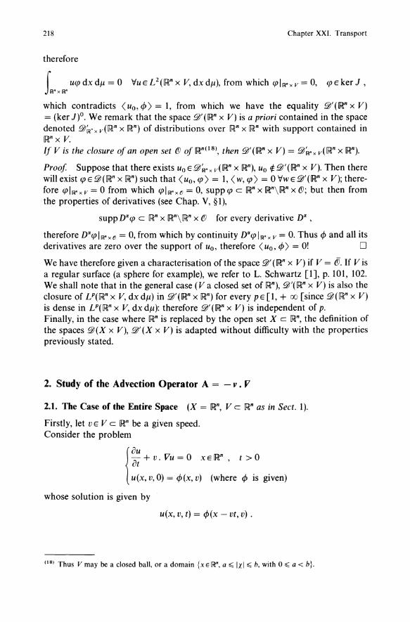
in other words t(x, v) is the time it takes a particle situated at x at t = 0 and having speed ( - v), to reach the boundary oX. This definition does not imply that the particle leaves the closed set X at time t(x, v) since the trajectory may be tangential to the boundary oX (see Fig. 1) when X is not
ax
Fig. 1
222 Chapter XXI. Transport
convex. For every cp E f0(X x V), we then define the operator G(t), t > 0, by:
(2.9) (G(t) 4> (x, v) = {4>(X -vt, v) ~f t < t(x, v) o If t ~ t(x, v)
for every (x, v) E X X V. (We can also eliminate the points (x, v) corresponding to trajectories tangential to ax, and therefore eliminate from X x V the set M of points (x, v) such that (x -t(x, v) v, V)E To; as the set To is of measure zero in ax x V, this will not have any influence in what follows). We have:
Theorem 2. The family of operators G(t), t > 0, defined by the relation (2.9) is extended into a semigroup of class riO in U(X x V), 1 ~ P < + 00. Further {G(t) }I;'O
is a contraction semigroup and operates in the cone of positive functions of LP(X x V). The generator of this semigroup is the operator A defined by the relations
(2.10) { i) D(A) = {UE WP; ul , = O} ii) Au = - v. Vu .
WP defined by (2.7)
Proof We shalI firstly show that for all cp E f0(X x V), we have
(2.11 ) lim IIG(t)cp -cpllu(xxv) = O.
By the density of f0(X x V) in U(X x V), (and {G(t)} being uniformly bounded), we deduce that {G(t)} is prolonged into a semigroup of class rio in U(X x V). Therefore let CPEf0(X x V). There exists to = to(4)) such that for all (x, v) in the support of 4>, we have t(x, v) > to(4)). We then have for t < to(4))
(2.12) II G(t)cp - cp II f,(x x V) = f I cp(x - vt, v) - cp(x, v)IP dx dJi(v) . xxv
We thus verify that (2.11) holds for all cp E f0 (X x V), from which (2.11) holds for all 4> E U(X X V) by density. We finally determine the generator of this semigroup. Let u be a function belonging to the domain of this generator and let cp E f0(X x V) be given. For t < to(4)) we have
(2.13) < G(t)u - u, cp> = f (u(x - vt, v) - u(x, v)) cp(x, v) dx dJi , xxv
and consequently
(2.14) 1. 1 . Im-(G(t)u-u)= -v. Vu III
1-0 t
For u to be in the domain of the infinitesimal generator (see Chap. XVII A, §2) we must have
(2.15) v. VUEU(X x V).
Finally if K is a compact set of T _, we verify that for all t > 0, G(t)u is zero in a neighbourhood of K. Thus G(t)uIK = 0 and the continuity of the trace mapping
§2. Existence and Uniqueness of Solutions of the Transport Equation 223
implies that UIK = o. We give a quick (and partially formal) justification of this. We use the characterisation of D(A):
(2.16) I. G(t)u - u .. ) ) 1m eXIsts In U(X x V <=> uED(A . t~O t
For every cpE~(X x V) and UE WP(X x V), we have:
(2.17)
f G(t)u(x, v)cp(x, v)dxd/1 = f u(x -vt, v)cp(x, v) Y(t(x, v) -t)dxd/1, xxv xxv
where Y denotes the Heaviside function; therefore:
(2.18)
/ _G_(t_)u_-_u ,cp) = f u(x', v) ~ [cp(x' + vt, v) Y(t(x', - v) - t) - cp(x', v)] dx' d/1, \ t xxv t
or even, by setting X(x', v, t) = Y(t(x', - v) - t), and by noting that:
v. VXlt=o = -v. vb(T+):
(2.19)
. (G(t)U -u ) f hm ,cp = uv. V(cpX)lt=odxd/1 t~O t x x v
= f u(v. Vcp)dxd/1 + f ucp(-v.vb(T+»dxd/1. xxv xxv
The use of Green's formula with II E WP(X X V), cp E ~(X X V) gives
(2.20)
f [u(v. Vcp)+(v. Vu)cp]dxd/1= r ucpv.vdy d/1- r ucplv.vldy d/1; xxv Jr. Jr
therefore, with dT = dy d/1:
(2.21) II·m (G(t)U - u , (fl) -- f f 't' -v. Vucpdxd/1- r_ ucplv.vldT.
t~O t x x v .
Thus, we obtain, for every cp E ~(X X V):
(2.22) II·m (G(t)U - u , (fl) -- f 't' - v. Vucp dx d/1 , t~O t xxv
if
(2.23) f_uCPlv.vldT=O, VcpE~(XXV), i.e. if ul r_ = o. We have therefore proved that the operator A defined above extends the generator.
224 Chapter XXI. Transport
Conversely if uED(A), we have for almost all (x, V)EX x V:
(2.24) (G(t)u - u)(x, v) = t G(s)( - v. Vu)(x, v) ds .
We deduce that A coincides with the generator of (G(t)),>o. The other properties stated in Theorem 2 are easily proved. o Remark 1. In L OO(X x V), G(t), t ~ 0 is also a contraction semigroup, but we have seen that it is not of class rt°. 0
Remark 2. If X is bounded and if 0 ¢ V (the modulus of the speeds is bounded from below by a strictly positive number), then the family of operators (G(t)) of Theorem 2 is null for large enough t. In effect in this case, there exists To > 0 such that
(2.25) t(x, v) ~ To, V(x, V)EX X V.
From which G(t) = 0 for t> To. The operators G(t) are nilpotent(22) for large t < To (we also say that the semigroup (G(t)) is nilpotent). From the physical point of view, the operator A corresponds to a problem (2.1) (with 1: = 0 and f = 0) where the particles propagate along straight lines, without shock in X. They escape from X when this straight line crosses ax (if X is convex). The time To is that for which all the particles represented by Uo in (2.1 )iii) have left X. 0
Remark 3. It follows from Theorem 2 that the advection operator A defined by (2.10) is an m-dissipative operator (see Chap. XVII A, §3, Theorem 9). This may be verified directly (we do this in the appendix in the more general case of the advection operator with reflection boundary conditions), which gives a new proof of Theorem 2, from the Lumer~Phillips Theorem (see Chap. XVII A, §3). The proof of the dissipative character of the operator A uses a Green's formula which is not directly applicable in the space WP(X x V), since the traces on r + and r _ , u I r +
and u I r of functions u E WP(X X V) are not necessarily in the spaces U(r ±, Iv. vi dy dll). We then introduce the space:
(2.26) WP(X x V) = {UE WP(X x V), ulr. E U(r +, Iv. vi dy dll)
and ul r EU(L),lv.vldydll)};
We can show (see Bardos [1] for p = 2, Cessenat [2J, for the general case) that
(2.27) WP(X x V) = {UE WP(X x V), ulr. EU(r+, Iv. vi dydll)}
= {UEWP(XX V),ul r EU(L,lv.vldydll)}
which also implies
(2.28) D(A) c WP(X x V) ;
we can then apply Green's formula for all u in WP(X x V) and therefore in D(A). In
(22) That is to say that for every t > 0, there exists n E I'\j such that (G(t)l" = O.
§2. Existence and Uniqueness of Solutions of the Transport Equation 225
the particular case p = 2, this formula becomes, for all u and WE WP(X x V):
(2.29)
f [U(v.VW)+(v.VU)W]dXdll=f UW1V.V1dYdll-f uwlv.vldydll· xxv r, r
We deduce immediately that A is dissipative in L 2(X x V), i.e.:
(2.30) (Au, u) ~ 0, VUED(A).
More generally, for functions dependent on time we are led to using a Green's formula (for p = 2) in the following framework, for r fixed > 0:
(2.31 ) OU
11'2 = {U E L 2(X X V x (0, r», ot + v. Vu E L 2(X X V x (0, r» ,
U(., 0)EL2(X x V), ulr~x(o.T)E L2(T _ x (0, r), v. vdydlldt)} .
The preceding results are again applied, by replacing
X and V by X x ]0, r[ and V x {l} respectively
(2.32) L by (Lx]O,r[)u(XxVx{O})
T+ by (Lx]O,r[)u(XxVx{O}).
Then for every U and WE 11'2, we have
(2.33)
fT [(U(t), v. Vw(t) + °ow (t») + (v. Vu(t) + °oU (t), w) ] dt o t U(XxV) t U(XxV)
= (u(r), w(r)b(xxv) - (u(O), W(0»L2(XXV)
+ f~«U(t)k' w(t)lr+>r+ - <u(t)lr~, w(t)IL>rJdt ,
denoting by <',>r, and <. >L the scalar products in L2(r+.lv.llldydll) and L2(L,lv.llldydll). D
Remark 4. The advection operator in the transport equation is the differential operator associated with the vector field (v, 0) of the space X x V (Note the change of sign from v to - v). In many applications from physics and mechanics, we meet differential operators associated with vector fields. The differential operator of the Vlasov equation is associated with a vector field (v, - Vx c1>(x». The differential operator of the Liouville equation is associated with the vector field denoted
( OH OH) (23) op , aq or ((lIm) VvH, - VxH) .
1 (23) The function H is called the Hamiltonian of the system considered; for H = -mv2 + <I>(x), where
2 <I> denotes the potential, we recover the vector field of the Vlasov equation.
226 Chapter XXI. Transport
In a general way (for 'regular' vector fields), if we associate the differential equation
dx dt = F(x) (F field of vectors) ,
with the linear partial differential equation:
au at+F(x).vu=O
(with solution u(t) = G(t)uo, t > 0), the results proved in this §2 in the particular case of a field (v, 0) can be extended (see Bardos [1]). We have therefore a step which takes a finite-dimensional (in x) nonlinear problem to an infinite-dimensional linear problem, the solution of the linear problem being obtained from the nonlinear problem by
u(x, t) = uo(e~tF(X)) = G(t)uo(x) ,
denoting by e~tF(x) = X(t) the solution of the nonlinear problem
dX - - 2 dt (t) = - F(X), X(O) = x( 4) •
This is a procedure frequently used in physics, and which is sometimes called Koopman's lemma (see Abraham-Marsden [1]). 0
3. Solution of the Cauchy Transport Problem
3.1. The Case of Absorbing Boundary Conditions
We shall now take into account the absorption terms and the collision terms which occur in equation (2.l)i) and which we have ignored up until now. In this Sect. 3.1, X will be an open set of IR", not necessarily bounded. If X = [R",
then ax = r + = r ~ = 0 and the boundary condition uk = 0 is omitted. We give first of all a perturbation result:
Proposition 2. Let A be the infinitesimal generator of a semigroup of class C(jO in U(X x V) (1 ~ p < + 00), 1: E L "'(X x V) be a given function and K a continuous linear operator from U(X x V) into itself; then the operator
(2.34) {i) T = A -1: + K
ii) D(T) = D(A)
is the infinitesimal generator of a semigroup of class C(jO in U(X x V). If, further, K and the semigroup generated by A operate in the positive cone of functions of LP(X x V), then the semigroup generated by T also operates in the cone of positive functions of U(X x V).
(24) This assumes that the nonlinear problem has a unique solution for t > 0, for (almost) all x.
§2. Existence and Uniqueness of Solutions of the Transport Equation 227
In what follows we are interested in the case
(2.35) A = -v. V
and we call T the transport operator, defined by
i) Tu(x, v) = - v. Vu(x, v) - L(X, v)u(x, v)
(2.36) + Ivf(x, v', v)u(x, v')dll(V'), uED(T) ,
ii) D(T) = D(A) (see (2.10), Theorem 2) .
In what follows we denote by G(t) = etA, Gdt) = etT = et(A-I:+K), t > 0., the semigroups in U(X x V) with infinitesimal generators A and T respectively.
Proof The first part of the statement is classical (see Chap. XVII A). We prove the second part: From Trotter's formula (see Chap. XVII B, §6), by using the exponential notation for semigroups, we have
t t t (2.37) et(A-I:+K) = lim (enAe-nI:enK)".
"-00
It is sufficient to show that each of the terms esA, e - sI: and esK operate in the cone of positive functions. This follows from the hypothesis for esA . Fore - sI:, this follows from the definition,
(2.38)
which is therefore a positive function since ¢ is positive. Finally ¢ ~ 0 implies by the hypothesis K¢ ~ 0 and K"¢ ~ 0; consequently
(2.39)
is positive. o We shall also use the following lemma.
Lemma 1. Let f(x, v', v) be a given real positive function (f~ 0), dll measurable in v and v'. We assume that there exist positive constants Ma and Mb such that
(2.40)
i) Ivf(X'V"V)dll(V)~ Ma , V(X,V')EXX V,
ii) Iv f(x, v', v) dll(V') ~ M b, Vex, v) E X X V .
Then the operator K defined by
(2.41) (Kcp)(x, v) = Iv f(x, v', v)cp(x, v') dll(V') , Vcp E U(X X V) ,
is linear, and continuous from U(X x V) into itself(pE[I, 00]).
228 Chapter XXI. Transport
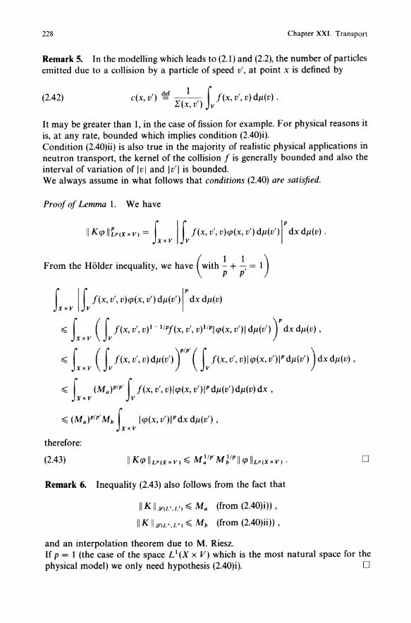
Remark 5. In the modelling which leads to (2.1) and (2.2), the number of particles emitted due to a collision by a particle of speed v', at point x is defined by
(2.42) def 1 r c(x, v') = l"(x, v') Jv f(x, v', v) dJl(v) .
It may be greater than 1, in the case of fission for example. For physical reasons it is, at any rate, bounded which implies condition (2.40)i). Condition (2.40)ii) is also true in the majority of realistic physical applications in neutron transport, the kernel of the collision f is generally bounded and also the interval of variation of I v I and I v'I is bounded. We always assume in what follows that conditions (2.40) are satisfied.
Proof of Lemma 1. We have
From the Holder inequality, we have (With! + ! = 1) p p'
L x v I L f(x, v', v)qJ(x, v') dJl(v' ) IP dx dJl(v)
~ Lxv (Lf(X, v', V)l-liPf(x, v', V)liPlqJ(x, v')1 dJl(VI»)P dxdJl(v) ,
~ Lxv (Lf(X, v', v)dJl(v' ) rp, (Lf(x, v', v)lqJ(x, vIWdJl(v' ) )dXdJl(V) ,
~ f (Ma)PiP' r f(x, v', v)lqJ(X, vIWdJl(v')dJl(v)dx , xxv Jv ~ (MayiP'Mb f IqJ(x, v'Wdx dJl(v') , xxv
therefore:
(2.43)
Remark 6. Inequality (2.43) also follows from the fact that
IIKII9'(LI.LI)~ Ma (from (2.40)i»,
II K 119'(L". P) ~ M b (from (2.40)ii» ,
and an interpolation theorem due to M. Riesz.
D
If p = 1 (the case of the space L 1 (X X V) which is the most natural space for the physical model) we only need hypothesis (2.40)i). D
§2. Existence and Uniqueness of Solutions of the Transport Equation 229
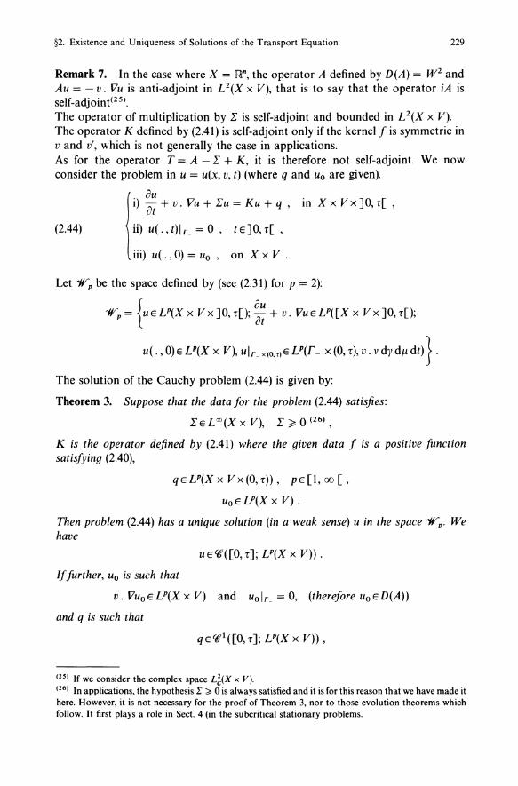
Remark 7. In the case where X = [Rn, the operator A defined by D(A) = W 2 and Au = - v. Vu is anti-adjoint in L 2(X x V), that is to say that the operator iA is self-adjoint(25). The operator of multiplication by 1: is self-adjoint and bounded in L 2(X x V). The operator K defined by (2.41) is self-adjoint only if the kernel f is symmetric in v and v', which is not generally the case in applications. As for the operator T = A -1: + K, it is therefore not self-adjoint. We now consider the problem in u = u(x, v, t) (where q and Uo are given).
au i) at + v. Vu + 1: u = K u + q, in X x V x ] 0, r[ ,
(2.44) ii) u(.,t)lr = 0, tE]O,r[,
iii) u(., 0) = uo, on X x V .
Let "flip be the space defined by (see (2.31) for p = 2):
"flip = {u E U(X X V x] 0, r[); ~~ + v. Vu E U( [X x V x] 0, r[);
u(. , 0) E U(X x V), ulr x (O.r) E U(r _ x (0, r), v. v dy dti dt) } .
The solution of the Cauchy problem (2.44) is given by:
Theorem 3. Suppose that the data for the problem (2.44) satisfies:
1: E L 00 (X x V), 1: ~ ° (26) ,
K is the operator defined by (2.41) where the given data f is a positive function satisfying (2.40),
qEU(XxVx(O,r)), pE[1,oo[,
UoEU(X x V).
Then problem (2.44) has a unique solution (in a weak sense) u in the space "flip. We have
UEct'([O, r]; U(X x V)) .
If further, Uo is such that
v. VUoEU(X x V) and uolr_ = 0, (therefore uoED(A))
and q is such that
(25) If we consider the complex space L~(X x V). (26) In applications, the hypothesis r ~ 0 is always satisfied and it is for this reason that we have made it here. However, it is not necessary for the proof of Theorem 3, nor to those evolution theorems which follow. It first plays a role in Sect. 4 (in the subcritical stationary problems.
230 Chapter XXI. Transport
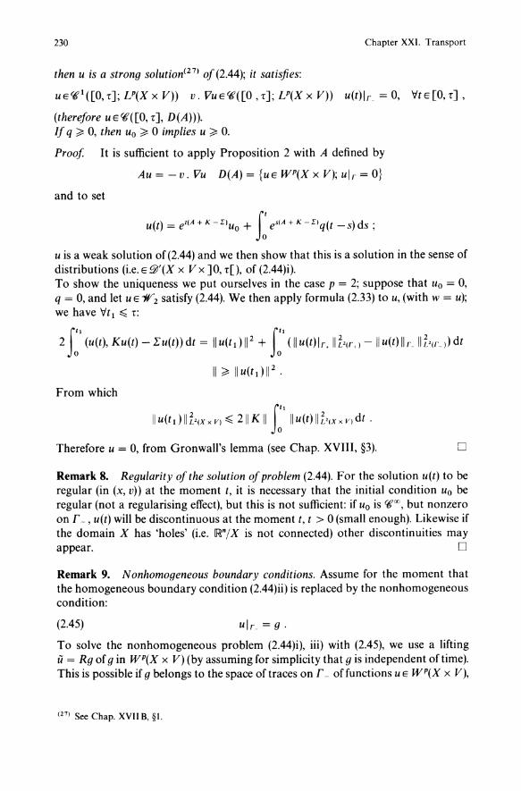
then u is a strong solution(27) of (2.44); it satisfies:
uErc1([0,r];U(XxV» V.VuErc([O,r];U(XxV» u(t)lr_=O, 'v'tE[O,r],
(therefore uErc([O, r], D(A))). If q ~ 0, then Uo ~ ° implies U ~ 0.
Proof It is sufficient to apply Proposition 2 with A defined by
Au=-v.Vu D(A) = {UEWP(XX V);ulr=O}
and to set
U(t) = eIIA+K-.[)uo + r esIA+K-.[)q(t -s)ds;
u is a weak solution of (2.44) and we then show that this is a solution in the sense of distributions (i.e. E ~'(X x V x ]0, r[), of (2.44)i). To show the uniqueness we put ourselves in the case p = 2; suppose that Uo = 0, q = 0, and let u E "IY2 satisfy (2.44). We then apply formula (2.33) to u, (with w = u); we have 'v't 1 :::::; r:
f l, ft. 2 0 (u(t), Ku(t) - L'u(t» dt = II u(t d 112 + 0 (II u(t)!r. II Z2Ir,) - II u(t) k II Z2(L) dt
II ~ Ilu(tdI1 2 .
From which
II u(t 1) II Z2(X x V) :::::; 211 K II f~' II u(t) II Z21X x V) dt .
Therefore u = 0, from Gronwall's lemma (see Chap. XVIII, §3). o
Remark 8. Regularity of the solution of problem (2.44). For the solution u(t) to be regular (in (x, v» at the moment t, it is necessary that the initial condition Uo be regular (not a regularising effect), but this is not sufficient: if Uo is rc oo , but nonzero on r _, u(t) will be discontinuous at the moment t, t > ° (small enough). Likewise if the domain X has 'holes' (i.e. IRn/x is not connected) other discontinuities may appear. D
Remark 9. Nonhomogeneous boundary conditions. Assume for the moment that the homogeneous boundary condition (2.44)ii) is replaced by the nonhomogeneous condition:
(2.45)
To solve the nonhomogeneous problem (2.44)i), iii) with (2.45), we use a lifting il = Rg of gin WP(X x V) (by assuming for simplicity that g is independent oftime). This is possible if g belongs to the space of traces on r _ of functions u E WP(X X V),
(27) See Chap. XVIIB, §1.
§2. Existence and Uniqueness of Solutions of the Transport Equation
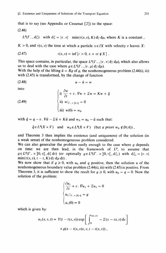
that is to say (see Appendix or Cessenat [2]) to the space:
(2.46)
U(L,d~) with d~ = Iv. vi min(t(x, v), K)dydJl, where K is a constant,
231
K > 0, and t(x, v) the time at which a particle x E ax with velocity v leaves x:
(2.47) r(x, v) = inf {t > 0, x + vt ¢X} .
This space contains, in particular, the space U(L, I v. vi dy dJl), which also allows us to deal with the case where 9 E U(r -, Iv. JlI dy dJl). With the help of the lifting il = Rg of g, the nonhomogeneous problem (2.44)i), iii) with (2.45) is transformed, by the change of function
(2.48) u-il=w
into I.) ow -~. at + v. Vw + Ew = Kw + q
11) wk x]O.t[ = 0
iii) w(O) = Wo
(2.49)
with q = q - v. Vil - Eil + Kil and Wo = Uo - il such that:
q E U(X X V) and Wo E U(X X V) (but a priori Wo ¢ D(A» ,
and Theorem 3 then implies the existence (and uniqueness) of the solution (in a weak sense) of the nonhomogeneous problem considered. We can also generalise the problem easily enough to the case where 9 depends on time: we are then lead, in the framework of LP, to assume that gEU(L x]O, t[, d~ dr) (or optimally gEU(L x ]0, t[, d~t) with d~t = Iv. vi min(t(x, v), t - t, K) dy dJl dt) . We now show that if 9 ~ 0, with Uo and q positive, then the solution u of the nonhomogeneous boundary value problem (2.44)i), iii) with (2.45) is positive. From Theorem 3, it is sufficient to show the result for 9 ~ 0, with Uo = q = O. Now the solution of the problem:
lOUt at + v. VUt + EUt = 0
Ut Ir_x]o.t[ = 9
udO) = 0
which is given by:
[ ('(X.V) ] Ut(x,v,t) = Y(t-t(x,v»exp Jo -E(x-vs,v)ds
x g(x - t(x, v)v, v, t - t(x, v» ,
232 Chapter XXI. Transport
is positive for positive g. By looking for the solution u of the problem
lou ot + v. Vu + 1:u = Ku
ul L x]O.<[ = g
u(O) = 0
in the form u = Ul + w, we verify that w is the solution of:
low iii + v. Vw + 1:w = K w + KUI
wi L x ]0. <[ = 0
w(O) = 0
Now Ul ~ 0 implies q = KUI ~ 0, therefore by Theorem 3, w is positive, therefore so is U(28). 0
3.2. An Integral Formulation of the Transport Equation
We restrict ourselves to the case of absorbing boundary conditions, we shall give an integral formulation of the transport problem (2.44), which we shall use for the spectral theory (§3) and which is the basis of numerous numerical methods. We start with the case analogous to (2.44) but without the right-hand side in (2.44)i).
Proposition 3. The solution u of the problem(29)
Ii) ~~ + v. Vu + 1:u = 0, t > 0 ,
ii) u(t)1 L = 0, t > 0 ,
XEX ,VE V ,
(2.50)
iii) u(O) = Uo
where Uo = uo(x, v) is given in U(X x V), p E [1, + 00], where 1: satisfies 1: E L ~ (X x V), is
(2.51 )
( ) = {uo(X - vt, v) exp ( - ft 1: (x + (s - t)v, v) dS) u x,v,t 0
o otherwise.
Proof For (x, v) E X x V and t > 0 fixed, set
U(s) = u(x + v(s - t), v, s)
1:(s) = 1:(x + v(s - t), v) ;
if x and x - vt E X
(28) This property can be considered as a variation of the maximum principle. (29) X and V mayor may not be bounded; we assume to simplify the exposition, that X is convex in this section.
§2. Existence and Uniqueness of Solutions of the Transport Equation 233
equation i) may be written
dU -ds(s) + I(s)U(s) = 0
the solution of which is
U(t)=u(o).exp ( - tI(S)dS).
By taking U(O) = uo(x - vt, v) null if x - vt ¢ X, we obtain the desired result. D
Remark 10. Formula (2.51) therefore explicitly gives us the semigroup GE generated by the operator A - I. When I is strictly positive (absorption), there is an exponential decrease in the solution u(t) of (2.50). D
Proposition 4. With the preceding hypotheses(30) on the given data I, f, uo and X, with q E U(X X V x ]0, r[), Vr > 0, the solution u of the transport problem (2.44) satisfies the following relation (called 'the integral formulation of the transport equation'):
(2.52) u(x, v, t) = uo(x - vt, v) exp ( - t I(x - vs, v) dS) Y(t(x, v) - t)
+ t exp ( - J: I(x - vr, v) dr) g(x - vs, v, t - s)
x Y(t(x, v) - s) ds
where
(2.53) g(x, v, t) ~f Iv f(x, v', v)u(x, v', t) dJl(v') + q(x, v, t) W (Ku + q)(x, v, t)
and Y is the Heaviside function (Y(s) = 0 if s < 0, Y(s) = 1 if s > 0).
Proof The transport equation (2.44) can be written in abstract form
du dt = (A - I)u + g .
By using the semigroup GE generated by the operator (A - I), we therefore have
u(t) = GE(t)uo + t GE(t - s)g(s) ds ,
from which we have the result by remarking that
GE(t)uo = uo(x - vt, v) exp ( - t I(x - vs, v) dS) Y(t(x, v) - t)
(30) See Theorem 3.
234 Chapter XXI. Transport
and that
f; Gr(t -s)g(s)ds = f; GJ:(s)g(t -s)ds. o
Remark 11. We can also demonstrate directly the existence of a solution of the transport equation, by showing that the integral equation (2.52) has a solution (see Papanicolaou [1]).
The method consists of making the change of variable
w(t) = e -.</ u(t)
with A ;?! 0 large enough, and showing that w is the solution of an integral equation analogous to (2.52)
(2.54) w = Bw + b
where B is a bounded operator. It can be shown that for A large enough, II B II < l. The solution of (2.54) is then given by the Neumann series:
w = L Bnb. n~O
This is a method analogous to that which we use in Sect. 4 to prove the existence in L 00 of a solution of the stationary subcritical problem. 0
Remark 12. We shall make explicit Remark II in the case uo E L "(X x V) and q = 0 (for simplicity). We define, from (2.52) and (2.53) a sequence of functions u(n)(x, V, t) in the following way:
dO)(x, v, t) = uo(x - vt, v) exp ( - f; L:(x - vs, v) dS). Y(t(x, v) - t)
u(n + I)(x, v, t) = u(O)(x, v, t) + r exp ( - t L:{x - vr', v) dr')
X Ku(n) (x - vs, v, t - s) Y(t(x, v) - s)ds.
We generally interpret these successive terms u(O), dl) - u(O), • •• ,dn + I) - d n) as representing the different generations of neutrons in probabilistic processes(31). Thus the term of order 0, UO(x, v, t) represents the evolution (of the density) of the initial neutrons, with attenuation due to the term:
exp ( - r L:(x -vs, V)dS) ,
the term of order 1, d I) - u(O) represents the evolution of the density of neutrons emitted at the first collision . .. We can also write the equations in a condensed form by
d n+ I) = dO) + Lu(n) from which d n+ I) _ dn) = L(dn) _ dn - I ») .
(31) We may also consider the adjoint equation (see Papanicolaou [I]. p. 27) which is, from the physical point of view, more natural for the framework of L" studied here (see also Sect. 3.3 and Remark 14).
§2. Existence and Uniqueness of Solutions of the Transport Equation 235
With the conditions:
1 0~ 1'(x,v)~ Ml < 00
o ~ i(x, v) = Iv f(x, v', v) dJ1(v') ~ M 2 < 00, l' ~ l' ,(32)
and the hypothesis: uo(x, v) is a bounded measurable function, we have the results:
if uo?! 0, then d n) ?! 0 .
With this hypothesis (i.e. Uo ?! 0), ,
u(O)(x, v, t) ~ II Uo II = sup ess I uo(x, v)1 . XxV
We can also show by induction that:
dn)(x, v, t) ~ II Uo II, '<In?! 0 and also by induction that:
u(n+ 1)(X, v, t) ?! dn)(x, v, t) .
We therefore have an increasing sequence converging to a function u(x, v, t) ?! 0 for Uo ?! 0, with u(x, v, t) ~ II Uo II. The theorem of monotone convergence implies that u(x, v, t) is a solution of (2.52), (2.53) (with q = 0). We can also demonstrate uniqueness (see Papanicolaou [1], p.26). Finally, we obtain, starting from the integral formula, the existence and uniqueness of the solution of the evolution problem in the framework of bounded, measurable functions. We have therefore a variant of Theorem 3(33). In the case where condition (2.l)ii) (or (2.44)ii)) is replaced by a nonhomogeneous condition:
u(x, v, t)IL = h(x, v, t), h given, bounded,
it is appropriate to change the right-hand side of expression (2.52) to
Y(t - t(x, v))exp [ - f~(x,V) l' (x - vs, v)ds]h(x - vt(x, v), v, t - t(x, v)).
This method may be equally well applied to an open bounded set X or in the whole space. (We refer for the details of this method to Papanicolaou [1]). In applications, we frequently use the integral transport equation, in particular in the spectral theory of the following paragraph and for numerical methods. 0
3.3. The Adjoint Transport Equation. Absorption Boundary Conditions
We begin with a fundamental remark. Take the same hypotheses and same notation as in Theorem 3. Then there exists afunction u, unique in "If""p, pE[l, 00 [,
(32) See also (2.67) and (2.70) for the analogous conditions. (33) The properties described below may be made precise with the help of semigroups as we shall see in what follows: under the hypotheses made (particularly i .;; 1") the family of mappings Uo -+ u(t), t > 0, in L 00 (X x V) is a contraction semi group, continuous for the weak star topology, and which preserves positivity.
236 Chapter XXI. Transport
and satisfying u E CC( [0, r]; U(X x V», which is the weak solution of the problem:
(2.55)
i) (~~ - v. Vu + 1:u) (x, v, t) = Iv f(x, v, Vi) u(x, Vi, t) dfl(V') + q(x, v, t) ,
ii) u(t)1,. = ° , iii) u(o) = UO, III X X V .
In effect, it is sufficient to replace v by - v, in the definition of the semigroup {G(t)} made in §2.3.1 and to replace f(x, Vi, v) by f(x, v, V' )(34). As in Proposition 4, we have an "integral formulation" of equation (2.55):
u(x, v, t) = uo(x + vt, v) (exp - L 1: (x + vs, v) dS) y(t(x, v) - t)
+ t exp ( - t 1:(x + vr, V)dr) g(x + vs, v, t - s) Y(t(x, v) - s) ds
for all t E [0, r], with
g(x, v, t) W Iv f(x, v, Vi) u(x, Vi, t) dfl(V' ) + q(x, v, t) .
On the other hand, we can see that the following operators are adjoint(35) respect-
'1' ( d' 11 [ IveytnUXxV)an U(XxV),-+-=l,pE]l,+oo: p pi
{
T = A - 1: + K with domain D(T) = D(A) = {UEU(XX V);v. VUEU(XX V),uir =o}
T' = A' - 1: + K' with domain D(T') = D(A') = {UEU'(X X V); v, VUEU'(X x V), uir, = o} ,
where A' and K' are given by: A'u = v. Vu, and
(2,56) K'u(x, v) = Iv f(x, v, Vi) u(x, Vi) dfl(V' ) ,
This fact allows us to deduce the existence of a weak solution of (2.55) from Proposition 2 and from general results on semigroups(36). We now study the particularly interesting cases p = 1 and p = 00: the case p = + 00 for the adjoint transport equation is the 'physically interesting' framework, since it is obtained by duality from the natural framework L 1 (X X V) of the (direct) transport equation (see Chap, I A, §5),
(34) Also replace V be - V = { - v, V E V}, dJl(v) by dJl( - v), and r", by r ±.
(35) In fact, here, the transpose. (36) See Chap. XVII A, §3, Theorem 5 for the case p = 2, and Butzer-Berens [1] for the other cases.
§2. Existence and Uniqueness of Solutions of the Transport Equation
We shall also make the following additional hypotheses here(37):
I i) L(x, v) ~ Iv f(x, v', v) d/1(v') ~ l"(x, v)
ii) i(x, v) ~ Iv f(x, v, v') d/1(v') ~ l"(x, v) .
Under hypothesis ii), the transport operator Tin L 1 (X X V) defined by;
{D(T) = {UE Wl(X x V), ulr = O} Tu = - v. Vu - l"u + Ku
237
is an m-dissipative operator (the fact that the operator T is dissipative in L 1 (X X V) follows from the proof given below of Proposition 5), and consequently is the infinitesimal generator of a contraction semigroup of class Cfio in L 1 (X x V), denoted (G 1 (t))t>o. Likewise, under hypothesis i) the operator T' in U (X x V) defined by:
{D(T') = {UE Wl(X x V), ulr = O} T'u = v. Vu -l"u + K'u
is an m-dissipative operator, and therefore the infinitesimal generator of a contraction semigroup of class Cfio in Ll(X x V), denoted (G'dtHr>o. We now go to the dual space L 00 (X x V) - The adjoint (transpose) semigroup of (G'dt)Lo, denoted here by (G'dt»1>o, is then a contraction semigroup in L OO(X x V), continuous in the weak star topology, with infinitesimal generator which is the adjoint(38) (transpose) of the operator T' above, denoted for the moment T'*. By definition:
D(T'*) ~ {u* E L 00 (X x V), such that 3g* E L 00 (X x V) ,
<T'u,u*) = <u,g*) VUED(T')}
and T'*u* = g*. Now it follows from the definition that if u* E D(T'*), v. Vu* (taken in the sense of distributions ~'(X x V)) belongs to L 00 (X x V), and by comparison with Green's formula (for all uED(T'»:
f (v.VU)U*dXd/1=f U(-V.VU*)dXd/1+f v.vuu*dyd/1 x x v x x v r = iJX x V
with the relation < T' u, u*) = < u, T'*u*) Vu E D( T') it also follows that f v.vuu*dyd/1=O VUED(T'), therefore u*lr =0. We thus verify that T'* is
identical to the transport operator T in the setting L 00 (X x V) with
{ T'*w = Tw = - v. Vw - l"w + K w
D(T'*) = {wELOO(Xx V),v. VWELOO(Xx V),WIL =O}
(37) Which we compare with hypotheses (2.67) and (2.70)i) made later for stationary problems. (38) See Butzer-Berens [1].
238 Chapter XXI. Transport
(Naturally the space WOO(X x V) ~ {uELOO(X x V), V, VUE L 00 (X x V)} has a trace on r± in LOO(r±» - Likewise the adjoint (transpose) semigroup of(G I (t»t>o, denoted here (G 1 (t»i>o, is a contraction semigroup in L OO(X x V), which is continuous for the weak star topology, with infinitesimal generator T*, with:
{ T*u = v. Vu -1:u + K'u
D(T*) = {UE WOO(X x V), ulr, = O}
that is to say the operator T' taken in the setting of L 00.
- These results allow us to solve problems (2.44) ('direct') and (2.55) (adjoint) in the frame-work L 00 (X x V) - which in turn allows us to recover the results of Remark 12 for (2.44) - by Picard's formula (see Chap. XVII B):
u(t) = G1 (t)uo + f~ G1 (t - r)q(r) dr t > 0,
[with G1(t) replaced by G1(t)* for problem (2.55)] for 'suitable' data Uo and q(39).
- Naturally, by interpolation, the semigroups (G 1 (t» and (Gdt)*Lo are contraction semigroups in U(X x V) for every p E [1, + 00], which completes (under hypotheses i) and ii» the study made beforefor pE] 1, + 00 [. Hypotheses i) and ii) are 'nonsupercritical' hypotheses: they imply that the spectra of the operators T and T' (for every p E [1, + 00]) a(T) and a(T') are contained in the half-plane {ZEC, Rez:S:; O}. Therefore they do not allow us to confirm that the operators T and T' are invertible - for this we must make stronger hypotheses which we shall see in the following section.
Green's Function. Besides the hypotheses already made in Theorem 4, we assume here that X and V are bounded with X convex, GJl the Lebesgue measure(40), and 1: E 'C(X x V), f E 'C(X x V x V). Then we can verify (by using the integral formulation and the fact that (x, v) -+ t(x, v) is a continuous mapping for convex X) that the solution u of (2.55) for q = 0 and Uo E 'C + (X x V) with:
(2.57) 'C+(Xx V) = {WE'C(XX V), wlr = O} equipped with the sup norm,
is such that u E 'C( [0, + 00 [, 'C + (X x V»; thus the family of mappings again denoted G 1 (t): Uo -+ u(t) in 'C + (X x V) for t ~ 0, is a semigroup of class 'Co in 'C + (X x V). Denote by vIt (X x V u r +) the space of bounded measures over (X x V) u r +
which is identified with the dual space of 'C + (X x V). Then the family of transpose (or adjoint) operators, denoted (Gt(t»t>o, of the operators (Gdt»t>o forms a 'weakly continuous' semi group over vIt (X x V u r + ) (that is to say continuous for the weak star topology of vIt(X x V u r +); see Butzer-Berens [1]). This
(39) For example uoEL"'(X x V), qE~O([O, + <X:J[. L:(X x V)) for a solution of (2.44) or (2.55) in a weak sense. (40) We shall assume (for example) for simplicity that V is a ball or domain Q( ,;;; Ivl < p.
§2. Existence and Uniqueness of Solutions of the Transport Equation 239
semigroup is the extension of the semigroup (Gi(t))t>o operating in LOO(X x V) obtained by duality from the semigroup (GdtHr>o operating in Ll(X x V). Let (Jo E..H(X x V u r +); then (J(t) ~ Gi(t)(Jo (which is a continuous function of t E [0, r] in ..H (X x V u r + ) for the weak star topology) is the solution of:
a(J , at - v. V(J + 1:(J - K (J = ° (2.58) (J(t)lr, = °
(J(O) = (Jo ,
in the following (weak) sense:
(2.59)
f: < (J(t), - ~~ + v. VI/1 + 1:1/1 - K 1/1) dt = < (J(r), l/1(r» - < (Jo, 1/1(0» (41)
for every function 1/1 E ~l ([0, r], ~ + (X x V» with TI/1 E ~O( [0, r], ~ + (X x V)). We choose, at present, 'I'(t) = u(r - t) with u the solution of (2.44) for UoE~+(XX V) (with TUoE~+(XX V». For (Jo = bxo . vo ' (the Dirac measure at (xo, vo) E X x V), let (Jxo. Vo be the solution of (2.58); (2.59) gives:
(2.60) < (Jxo. Vo (r), uo) - < bxo . Vo' u(r» = ° , or also:
(2.61)
which we write in the usual way:
u(xo, Vo, r) = f (Jxo. Vo (x, v, r) uo(x, v) dx dv ; xxv
(2.62)
Formula (2.62) allows us to interpret (Jxo. Vo as a Green's function of the transport problem (2.44).
Remark 14. In the physical plane, we show (see Bussac-Reuss [1]) that the solution (J(x, v, t) of the adjoint equation measures the importance of the neutrons at a given point, with given velocity, for a chain reaction and therefore, in particular, the response of a detector embedded in a part Qo of this medium. The adjoint problem is formally analogous to the problem related to the operator T(the direct problem). The advantage of the adjoint problem in applications is that it allows us to obtain in one calculation, the response which a detector gives to point sources (for example) at different points in the medium, with different velocities and intensities. 0
(41) The angle bracket < , > denotes the duality «j + (X x V), ,,(((X x Vu r +).
240 Chapter XXI. Transport
4. Solution of the Stationary Transport Problem in the Subcritical Case
All of the conditions which we give in this Sect. 4 are sufficient conditions for the solution of the stationary transport equation
{v. Vu + Lu = Ku + q, q given (positive) (42)
(2.63) with suitable boundary conditions .
Under these sufficient hypotheses, we shall see in §3 that the operator
(2.64) T=-v.V-L+K
will correspond to a subcritical case. We assume in all of these sections that L, K and q (and also the boundary conditions) do not depend on time t. Besides X or V mayor may not be bounded.
4.1. The Case of Absorbing Boundary Conditions
We put ourselves, first of all, in the case of the absorbing boundary condition (2.1)ii), u(x, v) = 0, V(x, v) E r _. By linear superposition (see Remark 9), it will be easy to deal with a nonhomogeneous boundary condition. Let A be an operator from U(X x V) into itself (1 ~ p < + 00) defined by
(2.65) {i) D(A) = rUE WP; ulr_ = O} (see (2.10)) ii) Au = - v. Vu .
Now let Q be the operator from U(X x V) defined by
(Qu)(x, v) = L(x, v)u(x, v) - Lf(X, v', v)u(x, v')dll(V').
We associate with (2.63), the following problem:
(2.66) {find u E D(A) such that - Au + Qu = q, with q given,
that is to say:
(2.66)' {v. Vu + Lu - Ku = q
uk =0.
As the operator - A is m-accretive and the operator Q is bounded (under the hypotheses of Theorem 3), we know(43) that for Re A large enough (Re A ~ II Q II), the equation
- Au + Qu + AU = q, q E U(X X V) given,
has a unique solution u E D(A). However, here, it is problem (2.66) in which we are interested and therefore the case A = O.
(42) Where K is always given by (2.41). (43) By the HiIle-Yosida theorem (see Chap. XVII A).
§2. Existence and Uniqueness of Solutions of the Transport Equation 241
In the case p = 2, for problem (2.66), with q E L 2(X X V) given, to have a unique solution, it is sufficient that there exists rx > 0, such that
( - Au + Qu, u) ~ rx II u 112
is true for all u E D(A). We return to the general case pE [1, + ex;].
Theorem 4. Adopting the hypotheses on the data J:, K, q, f, given in Theorem 3 to which we add:
i) J: and f satisfy (a.e. (x, v) E X X V)
(2.67)
i) J:(x, v) - Ivf(X, Vi, v)dJ!(v ' ) ~ rx
(X> ° , ii) J:(x, v) - Iv f(x, v, Vi) dJ!(v' ) ~ (X
ii) q does not depend on t and q E U(X X V). Then, (for p E [1, ex; [), problem (2.66) has a solution u in D(A) defined by (2.65) which is unique.
Proof(in the case p = 2).(44) As the operator - A is maximal accretive, we have:
(-Au + Qu, u,) ~ (Qu, u) Vu E D(A).
On the other hand, by using the Cauchy-Schwarz inequality, we notice that:
r u(x, v)u(x, v')f(x, x', v) dJ!(v' ) dJ!(v) ~ (r lu(x, v)1 2 f(x, Vi, v) dJ!(v) dJ!(VI))1/2 Jvxv Jvxv
( Iv x v I u(x, V')12 f(x, Vi, v) dJ!(v) dJ!(v') ) 1/2
Therefore by setting ga(x, Vi) = Iv f(x, Vi, v) dJ!(v), gb(X, v) = Iv f(x, Vi, v) dJ!(v' ) and
from hypothesis (2.67)
- (Qu, u) ~ Ix dX[ (Iv lu(x, V'W gb(X, Vi) dJ!(v' ) }/2 (Iv lu(x, vWga(x, V)dJ!(V)}/2
- Iv lu(x, vW J:(x, v) dJ!(v) ] ~ - rx II u II f2(X x V)
The operator (- A + Q) is maximal accretive and the result is a consequence of the Hille-Yosida-Phillips theorem. D
Remark 15. If rx = ° (the case excluded by Theorem 4) we again see that (A - Q) is the infinitesimal generator of a contraction semigroup of class Cfjo on L2(X x V). In
(44) For pE]I, + 00[, we are reduced to showing that - (QU,[U[p-2U)';; -1X[[u[[f"xxv)' which is proved in an analogous way to the case P = 2 with the help of Holder's inequality (replacing the Cauchy-Schwarz inequality).
242 Chapter XXI. Transport
the case where we can show that the semi group is of negative type(45) (for example if X is bounded and inf Ivl > 0), then we can again conclude the existence of
v E v a solution of problem (2.66). D
We recover Theorem 4 in the case p = 1, with the conditions: qELl(X x V) and only (2.67)ii)
Remark 16. Since L is assumed bounded, the hypothesis (2.67)ii) implies (besides L(X, v) > ex), that c defined by (2.42) satisfies
sup ess c(x, v) < 1 xxv
Conversely, with the hypothesis L(X, v) ? LO > 0 (LO constant) a.e. (x, v) E X x V, this condition implies (2.67)ii). This condition has the following physical interpretation: the number of neutrons created by the collision of a neutron of speed v at the point x (which has been denoted by c(x, v)) is (almost) everywhere less than a constant c C1:, strictly less than 1. Since in the case of inequalities (2.40) (see Remark 6), we only need hypothesis (2.67)ii) in the setting L 1 (X x V), and only hypothesis (2.67)i) in the framework L 00 (X x V). Hypotheses (2.67) are 'sub-criticality' conditions, that is to say that the spectra of the operators T and T', a(T) and a(T') are contained in the half-plane {ZEe, Rez:( - IX}, for all pE[I, + 00]. D
Proposition 5. Under the hypotheses on the data L, K, q stated in Theorem 3, in which we set p = 1, we add i) Land f satisfy (2.67)ii), ii) q does not depend on t and satisfies q ELI (X X V). Then the problem
(2.68) {i) v. Vu + LU - Ku = q ii) ulr_ = 0 (46)
has a unique solution in L I (X X V).
Proof Condition (2.67)ii) implies that the operator Q - ex is accretive in U (X x V). We show on the other hand that - A is also accretive in L I (X X V)(47) (and therefore m-accretive). As the operator Q is bounded, we deduce that - A + Q - IX is m-accretive and consequently that the problem
- Au + Qu = q
has a solution.
(45) See Chap. XVII A for this concept. (46) We shall denote the problem Tu = - q with (2.64) and (2.65). (47) Note that, as we indicated in Remark 3, we already know that the operator A is m-dissipative. We give here a direct proof of the fact that A is dissipative in L 1 (X X V).
§2. Existence and Uniqueness of Solutions of the Transport Equation
This follows from Green's formula (true for u E D(A))
(2.69)
now we have
where
f v. Vluldxdj.l(v) = r (v.v)luldT+ ;;::0; xxv Jr.
lui = usigno(u)
11 if u > 0 ,
signo = 0 if u = 0 ,
- 1 if u < 0 ,
is 'the duality mapping' of L I into its dual CC, see Chap. XVII A, §3.7. From (2.69), we therefore have
f (v. Vu)signo(u)dxdj.l(v);;:: 0 xxv
243
from which we have the fact that - A is accretive (see Chap. XVII A, §3). 0
To finish, we shall study problem (2.66)' in the space L ~(X x V). We have
Proposition 6. We put ourselves under the hypotheses on the data 1: and K stated in Theorem 3, and further assume that:
i) 1:(x, v') ;;:: 1:0 > 0 and:
ii) 1: and f satisfy (a.e. (x, v) E X X V)
(2.70) Lf(X, v', v)dj.l(v') ~ f31:(x, v), 0 ~ f3 < 1 (48)
iii) q does not depend on t and satisfies q E LX (X x V) .
Then problem (2.66)' has a solution u in Lox (X x V), which is unique.
Proof We shall show that the mapping which, to every ¢ E LX (X x V), associates the solution u E L etC (X X V) of
{ v. Vu + 1:u = K<p ul r _ = 0 ,
is a strict contraction II u II L OO(x x V) ~ f311 </> II L OO(x x V) with f3 < 1. Let
g(x, v) c;;r Lf(X, v', v)<p(x, v')dj.l(v') ;
(48) Since 1"(x, v) ~ 1"0> 0, condition (2.70)ii) is equivalent to condition (2.67)i). With 1", = inf (x. l') E X x v
1"(x, v), it is sufficient to take IX/(I - p) = 1", .
244
we have
(2.71 ) { v. Vu + 1:u = 9 ulr_ = 0 .
Chapter XXI. Transport
Now we can solve this problem by using the method of characteristics: we have
u(x,v)= t(x,V)exp ( - f~1:(X-VS,V)dS)9(x-vt'V)dt,
where t(x, v) is the travel time defined before (see (2.8)); we easily verify that the conditions gELOO(X x V), and (2.70)i) imply UE WOO (X x V)(49). By noticing then that
I I(X'V) ( II ) (g) u(x,v)= 0 exp - o1:(x-vs,s)ds 1:(x-vt,v) 1: (x-vt,v)dt
:::;: II~gll (1 - exp (- II(x, v) 1:(x - vs, V)dS)):::;: II~gll ' 1: L~(XxV) 0 1: L~(XxV)
we obtain the bound:
IluIIL~(XxV):::;: II~gll . £. L~(X x V)
Now
(~g }x, v) = 1:(~, v) tf(X, v', v)cp(x, v')d,u(v'}:::;: PII cp IIL~(xx V)
by the hypothesis, from which we have the stated result. Problem (2.66)' is then written, with the help of the operator B defined by
D(B) = D(A}, Bu = v, Vu + 1:u ,
in the form:
Bu = Ku + q
or even:
(1- B- 1 K)u = B- 1 q (50);
since we have shown that B- 1 K is a strict contraction in L 00 (X x V) (II B- 1 K II :::;: P < 1), this problem has a unique solution in L 00 (X x V). The solution of this problem may be obtained by iteration on the sequence un defined by
{ Bnun = K un - 1 + q D
u Ir_ = 0 .
Remark 17. The physical interpretation of the inequality in (2.70) can be made in terms of the importance of neutrons, in the framework of the adjoint transport equation.
(49) By taking p = 00 in (2.7), which has been excluded here. (50) Note that the existence of B- 1 follows from the solution of (2.71).
§2. Existence and Uniqueness of Solutions of the Transport Equation 245
We note that conditions (2.70)i) and ii) (equivalent to condition (2.67)i)) implies that the operators T' in L 1 (X X V) (with T' defined in section (3.3)) and Tin L 00 (X x V) have their spectra such that( 51):
a(T) = a(T') c {z d::, Re z ~ - a, a = (1 - f3)I: 1 = (1 - f3) inf I:(x, v)} x. v
Thus (2.70)i) and ii) are called 'sub critical' conditions of Tin L 00 (X x V). 0
4.2. Other Boundary Conditions
In the important physical case of nonhomogeneous boundary conditions, we establish the following result due to the maximum principle:
Proposition 7. We consider the following problem: find u satisfying
(2.72) {~~ v. Vu + I:u = Ku + q ll) ul, = g .
We adopt the hypotheses of Proposition 6 to which we add:
g is a positive function satisfying gEL GC (T _) .
Then problem (2.72) has a solution in L 00 (X x V); this solution is unique and satisfies (with 'Y. constant a > 0)
II u II 00 ~ sup( II g II 00' a II q Ila) (52) •
Proof We show the existence of u, the solution of (2.72), with q = 0, with the help of a fixed point theorem. Let UO be the solution (in L 00 (X x V)) of
{v. Vuo + I:uo = 0 ,
uOl, =g.
We obtain u as the limit in L 00 (X x V) of the sequence un defined by
Assume then that
We shall show that
{v. Vun + I:un = KU"-l
unl,_ = g .
II un II 00 ~ II g II ex; •
(51) The identity of the spectra of the operators T and T' (or T*) results from the property of the resolvents:
R(A, T*) = (AI - T*)-I = W - T)-I' = R(A, T)*
(see Butzer-Berens [I], p. 49 and Kato [I]). (52) In the setting of U(X x V) with P E [I, + eeL we have an analogous proposition for the existence and uniqueness of the solution of (2.72): by a lifting of the boundary conditions (2.72)ii) (see for this Theorem I of the appendix), we reduce this problem to (2.66)', resolved by Theorem 4.
246 Chapter XXI. Transport
Set
(2.73)
We have
( ft(x. ,') ) un(x, v) = exp - 0 l'(x - vs, v)ds g(x - t(x, v)v, v)
+ L(x"')exp ( - Ll'(X-VS,V)ds)qn-l(x-vt,V)dt;
now, the right-hand side is bounded by
f t(x. t') ( ft ) 111 II o exp - 0 l'(x - vs, v)ds l'(x - vt, v)dt l;qn-I ox
Now from the definition (2.73) of qn-I and the subcriticality hypothesis (2,70)i), we have
from which
Finally we have
(2.74) I un (x, v)1 ~ exp( - f~(x, ,') l'(x - VS, V)dS) Ilg II",
( ( f t(X' ,') ))
+ l-exp - 0 l'(x-vs,v)ds Ilgllw~llgll",
from which we have the result by recurrence. o
4.3. The Adjoint Transport Equation
Certain physical problems ask us to calculate the importance of the neutron population of particles situated at each point x for each speed, this leads to treating the following stationary problem: find u the solution of
{i,). - v. Vu + l'u = K'u + q, q given, (2.75)
11) ulr,=O,
with K'u(x, v) = Iv/(X, v, v')u(x, v')dJ!(v').
This problem is written, with the notation of section (3.3): find u E D(T) = D(A') satisfying:
(2.76) Tu = - q
§2. Existence and Uniqueness of Solutions of the Transport Equation 247
where the operator T' is the adjoint(53) of the operator T (see (2.64)). This duality between problems (2.66) and (2.76) may be justified from the physical point of view (see, for example, Bussac-Reuss [1] and Weinberg-Wigner [1]). We then have
Proposition 8. Under the hypotheses of Theorem 4 concerning the given data I, K, q,f and with p E [1, + 00], problem (2.75) has a solution in D(A'), where A' is the operator defined by
(2.77) {i) D(A') = {UE WP(X x V), ulr, = O} ii) A' u = v. Vu ,
and this solution u is unique.
Proof In effect, it is sufficient to change v to - v and f(x, v', v) to f(x, v, v') in the proof of Theorem 4 (in the case p = 2), or also to recall (see particularly Remark 16) that the conditions (2.67) imply that the operators T + Lt.! and T' + Lt.! are m-dissipative for all p E [1, + <Xl] and therefore a(T) = a(T') c {z E 1[, Re z ~ - Lt.}; thus the operators T and T' are invertible for all p E [1, + 00]. The interesting physical framework for the adjoint transport equation is (as for the evolution problem - see Sect. 3.3) that of the space L 00 (X x V). The condition (2.67)i) is then superfluous. D
Green's Function. We return to problem (2.75), with hypothesis (2.67). Assume that X is convex with X and V bounded, and dll the Lebesgue measure on V, and that IE CC(X x V), f E CC(X X V x V); we see, as in Sect. 3.4, that if q E CC + (X x V) = {WECC(X x V), wlr_ = O}, then problem (2.75) (or (2.75)') has a unique solution u E CC + (X x V) (the semigroup {Gdt)} in CC + (X x V) is then of negative type, and therefore its infinitesimal generator, again called T, has a bounded inverse). By duality the transpose operator, denoted here T*, in the space .A(X x V u r +) of bounded measures on X x V u r + (which is also the infinitesimal generator of the semigroup (GT(t)),> 0, continuous for the weak * topology) also has a bounded inverse (see for example Butzer-Berens [1], p. 49). Thus for all wE.A(X x Vu r.+) there exists eE.A(X x Vu r +) a solution of
(2.78) { -v. va + Ie = K'e + w
el l + = 0 ,
in the following weak sense:
(2.79) <e, v. VIjJ + IIjJ - KIjJ) = <w, 1jJ)
for every function IjJ E CC +(X x V) with TIjJ E CC + (X x V), the brackets < ) denoting the duality .A(X x V u r +), CC +(X x V). We choose in (2.79), <P = u the solution of (2.66)' (with q E CC +(X x V)) and e = 8xo • Vo the solution of (2.78) for W = bxo , Vo the
(53) In fact the transpose.
248
Dirac measure at (xo, Vo)EX x V; (2.79) then yields:
<<>xo. Vo' u) = <Oxo. Vo' q) ,
or again
(2.80)
which we write in the usual way:
u(xo, Vo) = f q(x, v)Oxo.vo(x, v)dxdv. xxv
(2.80)'
Chapter XXI. Transport
This allows us to interpret Oxo. Vo as a Green's function of the stationary transport problem (2.66)'; (2.80) expresses the solution u of (2.66)' directly as a function of the data q in C(j + (X x V).
Summary
In the resolution of evolution problems seen in Sect. 3, the solution u is written (in a Banach space Z, with for example Z = U(X x V), P E [1, + CI) D,
def u(t) = G1 (t)uo = exp(tT)uo ,
with
(2.81) II exp(tT) II ~ M 0 exp(wt)
where w is the type of the semigroup (see Chap. XVII A). If (2.81) is satisfied for one w < 0, then:
(2.82) II exp(t T)uo II --+ 0 exponentially VUo E Z .
In this case we can show (see Chap. XVII B, §2, Theorem 1) that
Tu = - q
has a unique solution u given by
u = fooo exp(tT)qdt .
In fact, in Sect. 4, we have sufficient conditions for (2.81) and (2.82) to hold. We have tried to give conditiops easy to satisfy in practice, such as (2.67) or (2.70). In particular, in the case (2.67), we have
w~ -(y,.
The ideas related to the asymptotic behaviour of the solution of the transport evolution problem will be studied in §3, Sect. 4 and will be linked to the ideas of subcriticality, criticality and supercriticality.
§2. Existence and Uniqueness of Solutions of the Transport Equation
Appendix of §2. Boundary Conditions in Transport Problems. Reflection Conditions
1. Explanation of Different Boundary Conditions in Transport Problems
249
1.1. Explanation of Absorbing Boundary Conditions. Let Xc [Rn(n = 3) be an open bounded convex set which we assume occupied by some medium (corresponding to given data L(x, v) and f(x, v, v'), X E X, v and v' E V), and placed in a vacuum. We assume that the initial density of neutrons in all the space [Rn is known, and we propose to determine the density of neutrons at the moment t, u(., t) in the space X (and in [Rn).
Let f and Jbe defined by: fix = L, fl~' x = O,]lx x Vx v = f,JI~'\x x Vx v = O. The transport problem in the whole space is written:
(1) li) au = Tu in [Rn x Vx ]0, + oo[ at
ii) u(O) = Uo in [Rn x V (54) ,
with. T the transport operator associated with f and J in [Rn x V. By using the fact that T(x, v, t) = - v. Vu(x, v, t) for x, VE([Rn\x) x V, we see also that if [x, x - vt] c [Rn\x, then
u(x, v, t) = uo(x - vt, v) ;
if xE[Rn\x with t(x, v) < t (where t(x, v) = oo{r, x - vrEX}), then:
(2) u(x, v, t) = h+(x - vt(x, v), v, t - t(x, v))
with h+ = ulr. x [0. + x[ .
Therefore for the part in the vacuum, the transport problem is reduced to finding the function h+ on r x [0, + 00[. For X, the transport problem reduces to
(3) 1 i) au = Tu in X x V x ]0, + 00 [
at
ii) u(O) = Uo Ix x v
iii) ul r = h- ,
with Tu = - v. Vu - Lu + Ku, and h- defined by:
(4) h-(x, v, t) = uo(x - vt, v).
the transport evolution problem (1) in the whole space reduces to the transport evolution problem (3) in X x V (X bounded and convex) with 'absorbing' boundary conditions, which are nonhomogeneous if we assume that some density of neutrons is crossing the vacuum at the initial instant, homogeneous if not. The solution of
(54) With the usual hypotheses in this §2 on uo, 1: andf, and particularly UoE W"(~n x V).
250 Chapter XXI. Transport
this problem allows us to determine the function h + (i.e. the density of neutrons leaving X), which gives the function U in the whole space.
1.2. Explanation of Reflection Boundary Conditions. We now consider two media, denoted 1 and 2, occupying domains X I and X z, with X I U X Z = ~n(n = 3), XI n X z = 0, and corresponding respectively to given data LI,fI; Lz,fz. The Cauchy problem of finding the neutron density u(x, v, t) in the whole space:
1 ~~ - Tu = 0 in ~n x V x ]0, + 00 [
(5) u(O) = Uo given in ~n x V (54) ,
(with T the transport operator associated with Land / defined by
Llx, = LI Llx2 = Lz,flx,xvxv' =/I,flx2xvxV' =/z)
is equivalent to the transmission problem:
(6)
i) a;/ - Tlul = 0 In XI x Vx]O, + oo[
1'1') auz ] [ -- Tzuz =0 In Xzx Vx 0, + 00 at
v) uz(O) = Uzo In X Z X V ,
with TI and Tz the transport operators associated respectively with L 1,11 and L z,fz. Suppose (for simplicity) that X I = X is bounded, and X 2 = ~n \ X; we use the notation r + and r _ to refer to X. The transmission problem (6) can be solved in the following manner: i) Firstly we solve the problem with nonhomogeneous absorbing boundary conditions:
(7) 1 i)
~~~ Uz (0) = Uzo m) uzk = h_
aUz -7it-Tzuz=O in (~n\x)xVx]O,oo[
in (~n\x) x V
on r _ x [0, + 00 [ ,
for all (assumed for the moment) given functions h _. The solution of (7) then determines the function h+ = uzl r• = RU20 (h-), ii) We then solve the problem with reflection boundary conditions:
aUI T . ] [ 7it - I U I = 0 In X X V x 0, 00
(8) UI (0) = UIO in X x V
ullr_ = RU20 (UllrJ on r _ x [0, + oo[ ,
§2. Existence and Uniqueness of Solutions of the Transport Equation 251
Condition (8)iii) follows from the transmission condition (6)iii): indeed, we have
ullr_ = u2lr+ = RU20(h_) = RU20 (U2Ir) = RU20 (Ull r J· The solution of(8) then determines uzlr_ = ullr+, therefore h_ in (7), from which we finally have the solution of (6), and therefore of (5). It must be noted that: i) the mapping denoted RU20:h- -> h+ is only linear(SS) if U20 = 0; ii) this mapping is not a priori local in x. This method of decomposition of the initial problem (5) may be interesting essentially if each transport operator Tl and T2 is very simple (for example L 1, II and L 2, 12 are constant over X 1 and X 2); particularly if the problem in the infinite region 2 can be simply resolved (the case of a vacuum, for example), then the problem in the whole space is reduced to a problem in an open bounded set.
2. The Advection and Transport Operators with Reflection Boundary Conditions
We propose to define the advection operator in U(X x V), pE[I, + 00[, for reflection boundary conditions, that is to say such that U Ir _ = R(u IrJ for a particular operator R acting from f + into 1 _ (to be made precise) in order to obtain an unbounded operator in U(X x V) denoted by AR with ARU(X, v) = - v. Vxu(x, v), which is the infinitesimal generator of a contraction semigroup of class reo in U(X x V). The difficulty in this definition lies in particular in the fact that for a pair of functions (g +, g _) defined over f + and f _, such that g _ = Rg +, there does not necessarily exist a function U E WP(X X V) such that on the one hand ulr. = g +, and on the other hand that g + and g _ are the traces on f + and f _ of the same function U E WP(X x V): for this we have to state some very precise trace theorems, giving the conditions relating g + to g _ for the existence of such a function U E WP(X X V). For a given operator from f _ to f + the problem will be to find (by restriction and closure) a reflection operator R satisfying the criteria below. Recall, first of all, the notation (see (2.46), (2.47)). For all (x, v) E 1 _ (resp. 1 +) we denote by r(x, v) the "time of travel" in X of the particle situated at x E ax, with the speed v, or:
if (x, V)Ef +: r(x, v) = inf{t > 0, x - vt ¢X} = sup{s > 0, x - vrEX, 'v'rE]O, s[} ,
if (x, V)El _: r(x, v) = inf{t > 0, x + vt ¢X} = sup{s > 0, x + vrEX, 'v'rE]O, s[} .
Thus for (x, V)El _, r(x, v) = r(x, - v). Let K be a positive constant; set TK(X, v) = min(T(x, v); K). The role of K is to eliminate "path" ("life") times which are too long in X (if X is bounded and if ° ¢ V, T(X, v) remains bounded for all (x, v) and we take TK(X, v) = T(X, v)). For pE I, + 00[, we denote by d~( = d~ ±) and d[,± the measures defined over f ± by:
{d~ = Iv. vlrK(x, v)dydll (9) d~~ =TK(x,v)I-Plv.vldydll=rK(x,v)-Pd~
(55) This is an affine mapping for u20 #- O.
252 Chapter XXI. Transport
(or d[~ = Iv. v I max (r(x, V)l-p, K')dydl1 with K' = K1-p; note that d~~ = I v . v I dy dl1). We therefore have the following inequalities and inclusions:
(10) {KPd[~ ~ Klv. vi dydl1 ~ d~ U(r ±,d[~)-+ U(r ±,Iv. vldydl1)-+ U(r ±,dO .
Let W~(X x V) = rUE WP(X x V), ulr, = O}. We can then state the trace theorem (see Cessenat [I], [2]):
Theorem 1. The trace mappings y ± : u -+ U I r are continuous and surjective with continuous liftingfrom WP(X x V) into U(r ±, dd andfrom W~(X x V) into U(r ±, d[~). 1 ~ p < 00.
This theorem allows us to solve the following problem: Find u E WP(X X V) satisfying:
(11) {v. V~ + AU = q ulr - u_ ,
for all q E U(X X V) and u _ E U( r _, d~) given (and where A denotes a constant, A > 0). We easily prove the existence and uniqueness of a solution of (I I), for example with the help of a lifting U E WP(X X V) of u_; by setting u = U + w, we are then reduced to the following problem in w:
{ v. Vw + AW = ij with ij = q - (v. VU + AU)EU(X x V) ,
wlr_=O,
from which we know the solution. It follows that the mapping u -+ (v. Vu + AU, ulr _) is an isomorphism from WP(X x V)
onto U(X x V) x U(r -, dO The explicit solution of (11) is given by
(12) u(x, v) = e-;'t(x.v)u_(x-t(x,v)v,v)+ Q(x,v), (X,V)EXX V,
with
(13) r(x.V)
Q(x, v) = Jo e-;'t q(x - tv, v)dt .
Now set, for (x, V)Er +:
Therefore Ro( = R~) is the mapping that takes every function u_ E U(r _, d~), into the trace u + = ulr + on r + of the solution u E WP(X X V) of the problem:
{v_. vu_+ AU = 0 in X x V (15)
ulr_ - u_ on r _ ,
and Ro is therefore a continuous mapping of U(r-,d~) (resp. U(r_,lv.vldydl1),
§2. Existence and Uniqueness of Solutions of the Transport Equation 253
U(r_,d[~)) into U(r_,d[) (resp. U(r+,v.vdydJl), U(r+,d[~)). This agam follows from Theorem 1 and the identity:
(16) WP(X x V) = {UE WP(X x V), ul r EU(r +, v. vdydJl)}
= {UE WP(X x V), ulr EU(L, Iv. vldydJl)} .
Likewise we set, for (x, v) E r +
(17) [r(x. v)
gl/oq(x, v) ~ Q+(x, v) ~ Jo e-J.tq(x - tv, v)dt;
fllo is therefore the mapping that takes every function q E U(X X V) into the trace Q+ = Vir. of the solution VE W~(Xx V) of
{v. VV_ + AV = q in ~ x V
Vir _ - 0 on r - , gl/o is therefore the continuous mapping from U(X x V) into U(r +, d~~), which is also surjective (from Theorem 1). We can therefore give the following trace theorem:
Theorem 2. Let (g+, g_)E U(r h d~) x U(r _, d~). There exists UE WP(X x V) such that ulr, = g+, Ur_ = g- if and only if(g+,g-) satisfies:
(18)
Proof i) Necessity: assume that there exists U E WP(X X V) such that U I,± = 9 ±. Let U be the solution of (15) for U _ = 9 _; then:
u - UE WP(X X V) and (u - u)lr_ = 0 therefore u - UE WHX x V)
and by restriction to r + we have the relation (18). ii) Sufficiency: if V denotes a lifting of 9 + - Rog _ into W~ (X x V), u = U + V E WP(X X V) and u Ir ± = 9 ±, from which we have Theorem 2. 0 We denote by f!{P the Banach space defined by:
(19) f!{P = {(g +, 9 _) E U(r h d~) x U(r _, d~) satisfying (18)} ,
with the norm II II'!"' given by:
(20) II(g+, g-)II~, = Ilg+ Ilf'(r+.dO + Ilg-llf'(r_.d¢) + IIRog- - g+ Ilf'(r .. d¢~)' We then have:
Corollary 1. The trace mapping y = (Yh y_):u --+ ulr = (ulr., ulr) is continuous and surjective, with continuous lifting from WP(X x V) into f!{P.
Note that for the definition of (19) and (20) we may have to use mappings other than Ro, for example the mapping Ro defined by
Rog-(x, v) = g_(x - r(x, v)v, v)x,(r(x, v)),
254
with () {o if r > f.
X r = , 1 if r ~ f.
(where I: denotes an arbitrary constant> 0). Let, now:
Chapter XXI. Transport
i) R be an unbounded operator of U(T +, dO into U(T _, d~); as usual we denote its domain and graph by D(R) and G(R), ii) AR be the advection operator defined in U(X x V). We can then state
(21 ) { ARU = - v. Vu D(AR) = {UE WP(X x V), (y+u, y_u)EG(R)} .
We shall note that !0(X x V) c D(A R) and therefore D(AR) is dense in U(X x V). We can then state:
Theorem 3. Assume that R satisfies the following conditions: i) the graph G(R) of R is a closed subspace of f1£P; _ ii) Im(1 - RoR) is contained and is dense in U(T +, d~~);
iii) there exists a constant C > 0 such that Vg + E D(R):
(22) 11(1 - RoR)g+ Ilu(/ •. d¢-~);?: C[ Ilg+ Ilu(/"d~) + II Rg+ Ilu( •. d¢)J ;
iv) D(R) n U(T +, v. vdydJ.l) is dense in D(R) equipped with the norm:
(23) Ilg+ IID(R) = (1Ig+ Ilu(/ •. d¢) + IIRg+ Ilu( •. d¢) + 11(1 - RoR)g+ Ilu(' .. dZ~))I/P;
v) R is a contraction for the measure I v. v I dydW Vg + E D(R) n U(T +, v. v dydJ.l)
(24)
Then the operator AR is the infinitesimal generator of a contraction semigroup of class ~o in U(X x V)(56).
Conversely, if AR is the infinitesimal generator of a concraction semigroup of class ~o in U(X x V) such that D(AR) n UiP(X x V) is dense in D(A R), then R satisfies properties i) to iv).
Corollary 2. If the hypotheses of Theorem 3 hold, the trace mappings y + and '{ y+:u---. ul •• , ylu---. (ul.+, ul.J are surjective with continuous extensions from D(AR) into D(R) and G(R) respectively.
We note that inequality (22) can be written in the form (with (9)):
(24)' r 1_(1_(1 - RoR)g+(x, V)IP d~;?: J •. 'K x, v)
C 1 [f.. Ig+(x, vWd~ + f.- IRg+(x, vWd~ J, Vg+ ED(R) ,
with C 1 constant, C 1 > 0, and with d~ = 'K(X, v)lv. vldydJ.l (see (9)).
(56) With D(AR) n J¥P(X x V) (see (16)) dense in D(A R) equipped with the graph norm, that is, the norm of W"(X x V).
§2. Existence and Uniqueness of Solutions of the Transport Equation 255
Proof of Theorem 2. We shall use in an essential way the Lumer-Phillips theorem (Chap. XVII A). i) The operator AR is dissipative over D(AR) n J.VP(X x V) if and only if v) is satisfied. The operator AR is dissipative for p > 1 if and only if we have (see Chap. XVII A, §3):
(25) (J(u), ARU) = f luIP- 2 u( - u. Vu)dxdJi:( 0, VUED(AR)' xxv
Now (see Chap. XVII A, §3):
u. V(luIP) = pluIP-1u. V(lul) = pluIP-1(signou)u. Vu = pluIP- 2uu. Vu.
Now we deduce by Green's formula:
(26) f lulp-2 U( - v. Vu)dxdJi = ~ f -v. V(luIP)dxdJi xxv P xxv
-~ f lulPv. vdydJi; p axx v
whence further, if u E D(A R) n J.VP(X x V):
(27) (J(u), ARU) = - ~ [f lu+ IPv . vdydJi- f lu-IPv. VdYdJi] ' P r. r
and consequently we have the equivalence:
(28) (J(u), ARU) :( ° -= II u_11 = II Ru+ Ilu(l_.lt"ld;odld:( II u+ 11L'lr •. l,d;dl'l .
In the case p = 1, we operate in the same way with J(u) = signo u (see Chap. XVII A, §3; see also in this §2, (2.69), (2.70» which again gives (28) for p = 1. ii) D(AR) n J.VP(X x V) is dense in D(AR) -= D(R) n U(T +, v. vdydJi) is dense in D(R). The trace mapping y +:u --+ uk is continuous from D(AR) onto D(A) (by Corollary 1) therefore we have the implication =. The converse is proved by constructing a lifting of D(R) into D(A R), which also proves Corollary 2; we set Q + = (I - Ro R)g + E U(T +, d[~) for all g + E D(R); Q + having a lifting U E W~ (X X V). Then set:
u(x, v) = e-).t(x.V) Rg+(x - t(x, v)u, v) + U(x, u), (x, V)EX X V.
We have UE WP(X x V) and ul r + = RoRg+ + Uk = RoRg+ + Q + = gh ulr_ = Rg +, therefore u E D(AR) and u is a lifting of g +.
D(AR) n J.VP(X x V)
i h+
Therefore properties i) and ii) which we have proved imply that AR is dissipative over D(AR)' iii) Im(I - AR) = U(X x V) if and only if hypotheses i), ii) and iii) are satisfied.
256 Chapter XXI. Transport
(This will imply that the operator AR is m-dissipative under hypotheses i) to v». We shall show the equivalence between: • (AI - A R) is an isomorphism from D(AR) onto U(X _x V) (for A > 0) . • (I - RoR) is an isomorphism of D(R) over U(T +, d~~).
The problem is to find U E D(A R) such that:
(29) (AI - AR)u = q, with q given in U(X x V) ,
that is to say such that:
(30) { i) v. Vu + AU = q, q E U(X X V)
ii) R(ulr,) = ulr
has, assuming for the moment that ulr = u_ is given, the solution (12); it then remains to show that relation (30) is satisfied, with (14) by taking the trace of u over T+ and by setting uk = u+, Qlr, = Q+ = rJPoq (see (17»:
(31 )
Since the set of Q + for ijU(X x V) is the space U(T +, d[~), we find that (30) has a unique solution u E D(AR) if and only if (31) has a unique solution u + E D(R )(the determination of u+ implying that of u _ = Ru+ and therefore of u by (12». From which we have the stated equivalence. But (I - Ro R) is an isomorphism from D(R) onto U(T +, d[~ ) if and only if the mappmg
!O:(U+,RU+)EG(R) -> (l-RoR)u+EU(T+,d[~)
is an isomorphism, or also if and only if conditions i), ii), and iii) of Theorem 3 are satisfied. [Indeed i) implies that D(R) equipped with the norm given by (23) is a Banach_space, and the mapping I - Ro R is continuous from D(R) into U(T +, d~~), with continuous inverse thanks to (22), therefore hypotheses i)
to iii) imply that (I - Ro R) is an isomorphism of D(R) onto U(T +, d[~), and in particular
Im(I - RoR) = U(T +, d[~) ;
the converse is done without any particular difficulty] 0 Generally, with a reflection operator R being defined as an unbounded operator from U(T +, d~) into U(L, d~), with a domain D, can we define a lifting of R with properties i) to v)? An answer to this question is given by:
Corollary 3. Let R be an unbounded operator from U(T +, d~) into U(T _, d~) satisfying properties ii) to v) of Theorem 3. Then the operator R has, "by closure(57»", an extension Ii. satisfying properties i) to v) of Theorem 3, and such that Ail is the infinitesimal generator of a contraction semigroup of class reO in U(X x V).
Proof The one thing to show is that R is closable, that is to say that the closure G of the graph G(R) of R in fIP is a graph, or: if fn E U(T +, d~), n EN, is a sequence
(57) In the sense that the graph G(R) is the closure of the graph G(R) in f!l7
§2. Existence and Uniqueness of Solutions of the Transport Equation
such that as n -> 00:
fn -> 0 in U(r +, d~), Rfn -> g_ in U(L, d~), (I - RoR)f,. -> - Rog - ,
then g_ = O.
257
Now from hypotheses ii) and iii), / - RoR has an inverse, denoted (1- RoR)-l, which is continuous over U(r +, d[~); therefore
(1- RoR)-l (I - RoR)fn = fn -> - (/ - RoR)-l Rog- ,
from which
(I - Ro R) - 1 Ro g _ = 0 ;
therefore Ro g _ = 0, and g _ = o. D
Now we shall give a fairly general type of reflection operator R satisfying inequality (22). First of all we remark (and this can be deduced easily from part i) of the proof of Theorem 3) that the operator Ro is a contraction operator from U(r -, I v. v I dy dl1) into U(r +, v. v dy dl1). Therefore if R is an unbounded (reflection) operator from U(r+,d~) into U(L,d~) and a contraction from U(r+,v.vdydl1) into U(L, Iv. vldydl1), i.e. satisfying (24), then RoR is a contraction operator in U(r +, V. v dy dl1). We then make the following slightly stronger hypothesis: iii)' Ro R is a strict contraction operator in U(r +, V. v dy dl1), (for ). = 1). We prove that if R satisfies iii)', iv) and ii), then R also satisfies iii), iv) v) and ii), and therefore R is a reflection operator over D(R) = (I - RoR)-l U(r +, d[~) such that AR is the infinitesimal generator of a contraction semigroup of class Cfjo in LP(X x V).
Proof The operator /-RoR has a continuous inverse in U(r+,v.vdydl1); consequently there exists a constant Co > 0 such that Vg + E D(R) n U (r+,v.vdy dl1):
(32)
By using the inequalities (10) and the fact that R is a contraction operator (see (24)), we obtain, for all Vg+ ED(R) n U(L, v. vdydl1)
K(P-l)/P( f, 1(1 - RoR)g+ IPd[~ YIP?: (If, 1(1 - RoR)g+ IP v . vdy dl1 yIP
Co ?: Co Ilg+ IIU(f,.vvdYdl')?: T[ Ilg+ IIL'(f"vvdydl') + II Rg+ IIU(L.lvvldydl')]
?: ~o K-1/P[llg+ IIU(f"d~) + IIRg+ IIU(L.d~)] ,
that is to say inequality (22) with C = Co/2K; the density hypothesis iv) then implies the stated result. We note that in this case D(R) c U(r +, V. v dy dll), and consequently that D(AR) c fVP(X x V) (with definition (16)).
258 Chapter XXI. Transport
We give several examples of a reflection operator local in x but not in v (see particularly Sentis [1]): i) the operator, called the specular reflection operator, defined by:
(33)
with rx a positive bounded function over ax, with 0 ~ rx ~ 1, which is 'naturally' defined over the space of bounded functions on r +. We can then verify that R is a contraction operator for the measure (V.11 )dydl1 (i.e. satisfies (24) with dl1 = dv). The operator RoR is given by:
(34)
RoRg+(x, v) = e-t(x.V) Rg+(x - r(x, v)v, v) = cp(x, v)g+(O(x, v)), (x, V)Er+
with ¢(x, v) ~f e - t(x. v) rx(x), (x, v) E r + (¢ is a positive function with 0 ~ ¢ ~ 1), and
with 8 the mapping from r + to r + :
(35) 8(x, v) = (x', w), x' = x - r(x, v)v, w = v - 2(vx"v)vx';
8 is therefore the 'billiard' mapping (for n = 2) - see for example Arnold-A vez [1], pp.201-202. Naturally if the function rx satisfies 0 ~ rx(x) ~ rxo < 1, then RoR is a strict contraction operator in U(r +, V. v dy dv); inequality (22) is therefore satisfied, and R (with
D(R) ~ (/ - Ro R) - 1 U(r +, v . v dy dv)) defines an operator A R which is the infini
tesimal generator of a contraction semigroup in U(X x V). (The condition that rx is bounded by rxo < 1 is not necessary for the above result; it must essentially satisfy (22) or (22)'); ii) the integral reflection operator defined by:
(36) Rg+(x, v) = L.g+(x,w)n(x.v)(dW), (x,v)EL,
where rx+ = {VE V, V. Vx > O}, n(x. v) is a positive bounded measure over r x+, with total mass ~ 1, depending on (x, v) E r _. The specular reflection operator is a special case of this operator with:
n(x.v)(dw) = rx(x)bv - 2 (v x .,')vjw);
another particular case is given by the isotropic reflection operator, where
n(x. v)(dw) = rx(x)vx · wdl1(w) I f". VX ' wdl1(w)
(with 0 ~ rx(x) ~ 1). Under fairly general hypotheses on the operator R (see for example Sentis [1]) we can define an advection operator Ail in U(X x V)~ with R the reflection operator which is a lifting of the given operator R. We refer, for further details, to Sentis [1]<58). D
(58) But note that inequalities (22) must be satisfied.
§2. Existence and Uniqueness of Solutions of the Transport Equation 259
Remark 1. We emphasise the generality of Theorem 3: it is not necessary to assume X and V bounded, nor R to be a local operator in x, nor p = 2; the choice of framework U, p E [1, + 00 [ has been made according to the framework chosen in §2 for the advection operator A with absorbing boundary conditions. The framework L 1, which is natural for the physical model, involves some notable simplifications since d[~ = v. vdydll. We can again generalise Theorem 3, in the case where R is not a contraction, to obtain, by the Hille-Y osida theorem, a necessary and sufficient condition on R for AR to be the infinitesimal generator of a semigroup of class rcO in LP(X x V). 0
Remark 2. Positivity. We note that the operator Ro defined by (14) is positive, i.e.:
(37)
(for all A > 0); consequently if R is also a positive reflection operator, Ro R is also a positive reflection operator. In the case where Ro R is also a strict contraction operator in U(T +, v . vdydll) (for A = 1 for example), then equation (31) has, for all given Q + ~ ° with Q+EU(T+,d[~), a unique solution U+, with U+ ~o. This immediately implies that for given q ~ ° with q E U(X x V), the solution U of problem (30) (for A = 1 here) is also positive. We deduce that the contraction semigroup (GR(t))t~O with infinitesimal generator AR is positive(S9), that is to say that:
(38)
this follows from the formula (see Chap. XVI and XVII)
GR(t)uo = etARuo = lim (I -~AR)-n Uo, t > 0. n-x) n
We can now consider the Cauchy problem for the transport equation with reflection boundary conditions:
in X x Vx ]0, r[ (39) {
aaUt + v. Vu + LU = Ku + q
u(.,t)lr_ =R(u(.,t)lrJ on T_x]O,r[
u(O) = Uo in X x V,
with the given data uoED(AR), qErc1 ([0, r], U(X x V)) (or more generally Uo E U(X x V), q E U(X x V x ]0, r[)), under the hypotheses of Theorem 3(§2) on Land K. The transport operator TR with reflection boundary conditions defined by:
(40) { D(TR) = D(AR) TRu = ARu - LU + Ku, uED(AR),
(59) We note that the supplementary condition that Ro R is a contraction is certainly not necessary for the semigroup (GR(t)),;,o to be positive.
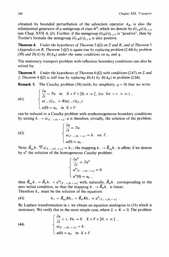
260 Chapter XXI. Transport
obtained by bounded perturbation of the advection operator AR , is also the infinitesimal generator of a semigroup of class C€o, which we denote by (G 1 R (t», ;> 0
(see Chap. XVII A, §3). Further, if the semigroup (GR(t)b 0 is "positive", then by Trotter's formula the semigroup (G IR (t)),;> 0 is also positive.
Theorem 4. Under the hypotheses of Theorem 3 (§2) on 1: and K, and of Theorem 3 (Appendix) on R, Theorem 3 (§2) is again true by replacing problem (2.44) by problem (39) and D(A) by D(AR) under the same conditions on Uo and q.
The stationary transport problem with reflection boundary conditions can also be solved by:
Theorem 5. Under the hypotheses of Theorem 4 (§2) with conditions (2.67) on 1: and f, Theorem 4 (§2) is still true by replacing D(A) by D(AR) in problem (2.66).
Remark 3.
(41)
The Cauchy problem (39) (with, for simplicity, q = 0) that we write:
{
~~ = Tu in X x V x] 0, + 00 [, (i.e. for r = + 00) ,
u(.,t)lr_ =R(u(.,t)lrJ
u(O) = Uo in X x V
can be reduced to a Cauchy problem with nonhomogeneous boundary conditions by setting h - = u I r _ x ]0. + 00[: u is therefore, trivially, the solution of the problem:
at { au = Tu
(42) ulr_x]o.+oo[=h- on r-u(O) = Uo .
Note: Ruoh- ~ ulr + x[O, + w[ = h+; the mapping h_ -+ Ruoh- is affine: if we denote by UO the solution of the homogeneous Cauchy problem:
{
auo -= Tuo at
u:1r _ x]O. + oo[ = 0
u (0) = Uo , - - 0 -then RuoL = Roh- + u Ir+ x]O,+oo[ with, naturally, Roh- corresponding to the
zero initial condition, so that the mapping h _ -+ Ro h _ is linear. Therefore h+ must be the solution of the equation:
(43)
By Laplace transformation in t, we obtain an equation analogous to (31) which is stationary. We verify this in the most simple case, where 1: = K = O. The problem
{ ~~ + v. Vu = 0 X x V x ] 0, + 00 [ ,
(44) ulr- x]O. +oo[ = h_
u(O) = Uo in X x V
§2. Existence and Uniqueness of Solutions of the Transport Equation
has for solution(60):
(4S) u(x, v, t) = Y(t - t(x, v»h_(x - t(x, v)v, v, t - t(x, v»
+ Y( - t + t(x, v»uo(x - tv, v) ,
which yields for (x, v) E r +, by setting h + = u I r + x ]0, + CXj(
(46) h+(x, v, t) = Ruoh_(x, v, t) = Y(t - r(x, v»h_(x - r(x, v)v, v, t - r(x, v»
+ Y( - t + t(x, v»uo(x - tv, v) .
By Laplace transformation in t, we obtain, with the notation:
(47) ff(X'V)
Q+(V,V,A)= ° uo(x-vt,v)e-)./dt, A>O,
(48)
261
which is equation (31 )(61) in Ii + with Ii_replaced by Rli +; this equation has for each A> 0, a unique solution Ii+(., A) in D(R) from Theorem 3 (Appendix), which, by inverse Laplace transformation gives h+(x, v, t) and by (4S) with h_ = Rh+. the solution of the Cauchy problem with reflection:
{ ~~ + v, Vu = ° in X x V x ] 0, + c:f.) [ ,
(49) ulr_ x]O, +x[ = R(ulr+ x]O,+X
262 Chapter XXI. Transport
we easily obtain (again denoting by K' the transpose of the operator K):
(52) T~w = v. Vw - 17w + K'w, VWED(T~) c WP'(X x V).
By Greens's formula(62), we must have:
(53) (TRu, w> - (u, T~w> = - t v.nuwdydfl = 0,
therefore for all u I r + E D(R), w must be such that:
(54) - r v.nuwodydfl + r Iv.nIRulr_ Wdydfl = 0, Jr+ Jr-or again, with the notation
(u, w>r+ = f v.nuwdydfl (u, w>r_ = f Iv.nluwdydfl, T+ r+
(55) (Ru, w>r_ - (u, w>r+ = 0, Vulr+ ED(R) ,
which implies wlr+ = R'(wlr_ ED(R'), R' being the transpose of R(63). We know (see Chap. XVII A, and Butzer-Berens [1]) that for P E] 1, + 00 [resp. = 1), T~ is the infinitesimal generator of a contraction semigroup of class Cfjo (resp. continuous for the weak* topology), which implies the existence and uniqueness of the solution u of problem (2.55) where condition (2.55)ii) is replaced by u(t)lr+ = R'(u(t)lr_), tE]O, r[.
§3. Spectral Theory and Asymptotic Behaviour of the Solutions of Evolution Problems
1. Introduction
We intend to study here the spectrum of the operator T defined by
3.1) {i) Tu = - v. Vu - 17u + Ku ( ii) D(T) = {UEU(X x V), v. VUEU(X x V), ulr_ = OJ, pE[I, 00 [
with (2.2), and the usual conditions of §2, I" and.f positive functions(64), I" E L 00 (X x V), and (2.40).
(62) Written a priori formally, which naturally may be justified. (63) Recall that G(R) is a closed subspace of .srp (see Theorem 3. Appendix). and G(R') is therefore the annihilator of G(R) (see for example Butzer-Berens [1], p, 46). (64) As we have indicated in §2, this positivity hypothesis of L andf, which is natural in the framework of transport problems, can be eliminated in numerous cases, as in the case of a Boltzmann equation which can be linearised in the vicinity of a Maxwell function; on the other hand the positivity hypotheses will be essential in the study of the beginning of the spectrum of T for the application of the Krein-Rutman theorem, and the spectral results which follow are then very different. Whereas the eigenvalue with largest real part of T, Ao(T) will be simple (in the "usual" case), it will not be the same for the operator TB: for examples related to this operator with periodic boundary conditions we refer to Palczewski [I] where Ao(TB ) has multiplicity five.
§3. Spectral Theory and Asymptotic Behaviour of the Solutions of Evolution Problems 263
In fact, in most cases we restrict ourselves to the space L2(X x V)(65) because this is the most simple. We shall only treat, in this §3, the case of absorbing boundary conditions. We shall generally put ourselves in the position where V is either a nonempty closed subset of ~n which may contain the origin or not (with V = V and with the Lebesgue measure), or a union of spheres (multigroup case) with surface measure. The operator T does not have any of the properties for which specific elements of the spectral theory were worked out in Chap. VIII. It is neither self-adjoint, nor normal and its resolvent is not compact. The particular study which we make here of its spectrum will lead us to understand the asymptotic behaviour of the solution of the problem
(3.2) {i) du = Tu (66)
dt
ii) u(O) = Uo
Indeed consider the following cases, of increasing difficulty concerning the semigroup generated by an operator A and the asymptotic behaviour of (etA)uo: 1) Assume that A is a matrix in ~n with eigenvalues At. ..1.2 , ••• , An' i) If these eigenvalues are simple, or if their algebraic multiplicity is equal to the geometric multiplicity, then we have the relation
(3.3) n
etA = LetA, Pk , k=i
where Pk is the projector over the eigenspace of Ak in ~n. This gives the asymptotic expansion as t ~ + 00 , and for Uo E ~n:
(3.4) (etA )Uo = LetA, PkUo + O(e~t) . Re).k>/Z
ii) If the eigenvalues of A have algebraic multiplicity greater than their geometric multiplicity, we must modify formula (3.3).
Example 1. If A = (~ ~). then by setting B = (~ ~). we have:
etA = etAetB = etA(l + tB) . o In case ii) we obtain an asymptotic formula of type rx (for t ~ + 00 )
(3.5)
where PI:' is a projector in ~n.
(65) This space will be taken complex for the spectral study of this §3. Note that we can show in numerous cases (see for example Mokhtar-Kharroubi [1], Palczewski [1]) that the point spectrum of T is independent of the choice of pE [1, 00 [ in U(X x V).
du (66) Or more generally - = Tu + q with lim q(t) = qoo in the space considered.
dt 1-++00
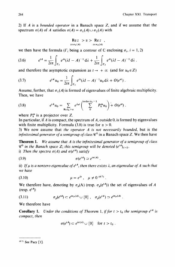
264 Chapter XXI. Transport
2) If A is a bounded operator in a Banach space Z, and if we assume that the spectrum a(A) of A satisfies a(A) = adA)u az(A) with
Rez >!Y. > Rez , ZEal (A)
we then have the formula (Ti being a contour of <C enclosing ai, i = 1,2)
(3.6) etA = ~ f eAt(AJ - A)-l dA. + ~ f eAt(AJ - A)-l dA. . 2m T, 2m T2
and therefore the asymptotic expansion as t --+ + 00 (and for Uo E Z)
(3.7) etAuo = ~ f eAt(Al_ A)-luodA. + O(e~t). 2m T,
Assume, further, that a 1 (A) is formed of eigenvalues of finite algebraic multiplicity. Then, we have
(3.8)
where PI:' is a projector over Z. In particular, if A is compact, the spectrum of A, outside 0, is formed by eigenvalues with finite multiplicity. Formula (3.8) is true for 0( > O. 3) We now assume that the operator A is not necessarily bounded, but is the infinitesimal generator of a semigroup of class C(;jO in a Banach space Z. We then have
Theorem 1. We assume that A is the infinitesimal generator of a semigroup of class C(;jO in the Banach space Z; this semigroup will be denoted (etA)t > o.
i) Then the spectra a(A) and a(etA ) satisfy
(3.9)
ii) If J1 is a nonzero eigenvalue of etA, then there exists A., an eigenvalue of A such that we have
(3.l 0) J1 = eAt, J1 ¥- 0 (67) •
We therefore have, denoting by ap(A) (resp. ap(etA )) the set of eigenvalues of A (resp. etA):
(3.l1 )
We therefore have
Corollary 1. Under the conditions of Theorem 1, if for t > to the semigroup etA is compact, then
a(etA ) c eta (A) u {O} for t > to .
(67) See Pazy [1].
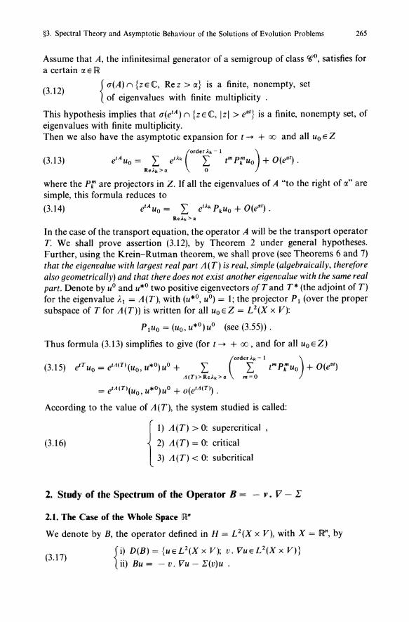
§3. Spectral Theory and Asymptotic Behaviour of the Solutions of Evolution Problems 265
Assume that A, the infinitesimal generator of a semigroup of class I(j0, satisfies for a certain (X E IR
(3.12) { u(A) n {z E C, Re Z > (X} is a finite, nonempty, set of eigenvalues with finite multiplicity .
This hypothesis implies that u(etA)n{zEC, Izi >e«t} is a finite, nonempty set, of eigenvalues with finite multiplicity. Then we also have the asymptotic expansion for t -+ + 00 and all Uo E Z
(3.13)
where the Pt:' are projectors in Z. If all the eigenvalues of A "to the right of (x" are simple, this formula reduces to
(3.14) etAuo = L et)..k PkUo + O(e«t) . Re)..k>«
In the case of the transport equation, the operator A will be the transport operator T. We shall prove assertion (3.12), by Theorem 2 under general hypotheses. Further, using the Krein-Rutman theorem, we shall prove (see Theorems 6 and 7) that the eigenvalue with largest real part A(T) is real, simple (algebraically, therefore also geometrically) and that there does not exist another eigenvalue with the same real part. Denote by UO and u*o two positive eigenvectors ofTand T* (the adjoint of T) for the eigenvalue Al = A(T), with (u*o, UO) = 1; the projector PI (over the proper subspace of T for A(T» is written for all Uo E Z = L 2(X x V):
P1Uo = (uo, u*O)UO (see (3.55» .
Thus formula (3.13) simplifies to give (for t -+ + 00, and for all Uo E Z)
(3.15) etT Uo = etA(T) (uo, u*O)UO + L (OrdeIk-l tm Pt:'uo) + O(e«t) A(T»Re)..k>« m=O
= etA (T)(UO, U*O) UO + o(etA(T» .
According to the value of A(T), the system studied is called:
{I) A(T) > 0: supercritical ,
(3.16) 2) A(T) = 0: critical
3) A(T) < 0: subcritical
2. Study of the Spectrum of the Operator B = - v. V - L
2.1. The Case of the Whole Space IR"
We denote by B, the operator defined in H = L 2(X x V), with X = IR", by
(3.17) {i) D(B) = {uEL2(X x V); v. VUEL2(X x V)} ii) Bu = - v. Vu - .r(v)u
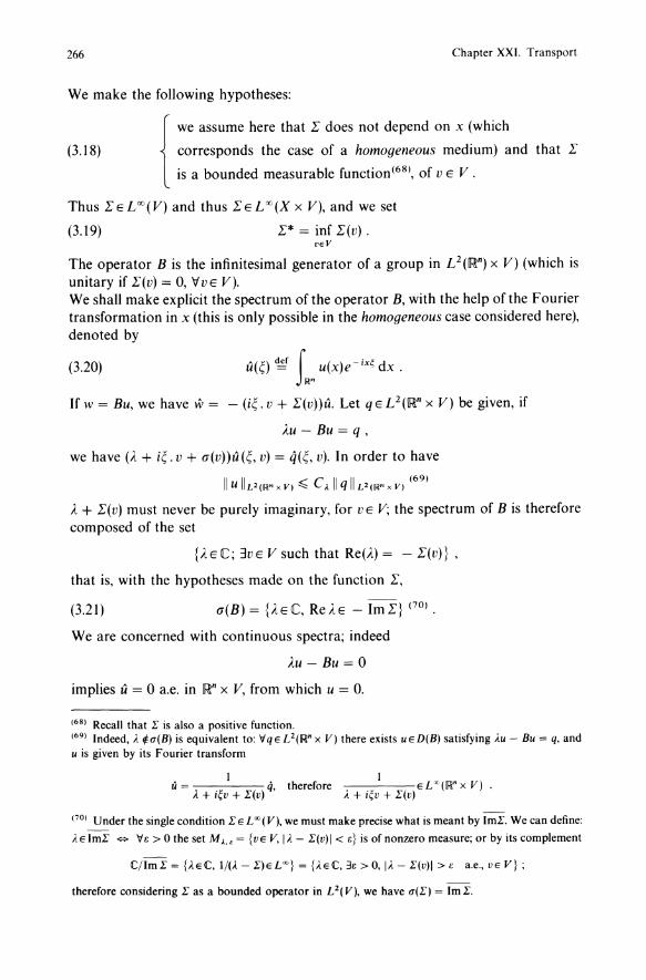
266 Chapter XXI. Transport
We make the following hypotheses:
(3.18) {we assume here that L: does not depend on x (which
corresponds the case of a homogeneous medium) and
is a bounded measurable function(68), of v E V.
Thus L:ELOO(V) and thus L:ELOO(Xx V), and we set
(3.19) 1:* = inf L:(v) . t'EV
that L:
The operator B is the infinitesimal generator of a group in L2([Rn) X V) (which is unitary if L:(v) = 0, VVE V). We shall make explicit the spectrum of the operator B, with the help of the Fourier transformation in x (this is only possible in the homogeneous case considered here), denoted by
(3.20) A (I') der i () ~ ix¢ d u",= uxe x. n;ln
If w = Bu, we have w = - (i~. v + L:(v))u. Let q E L 2([Rn X V) be given, if
AU - Bu = q,
we have (A + i~. v + IT(v))u(~, v) = q(~, v). In order to have
II u II U(n;ln x V) ~ c,\ II q II U (n;ln X V) (69)
A + L:(v) must never be purely imaginary, for v E V; the spectrum of B is therefore composed of the set
{AEC; 3VE V such that Re(A) = - L:(u)} ,
that is, with the hypotheses made on the function L:,
(3.21) IT(B) = {AEC, RdE - ImL:} (70) .
We are concerned with continuous spectra; indeed
AU - Bu = 0
implies u = 0 a.e. in [Rn x V, from which u = O.
(68) Recall that 1: is also a positive function. (69) Indeed, Ie ~u(B) is equivalent to: If q E e(~" x V) there exists U E D(B) satisfying ;.u - Bu = q, and u is given by its Fourier transform
11- 1 . - Ie + i~v + 1:(v) q, therefore
1 -:-----EC(~"X V) . Ie + i~v + 1:(v)
(70) Under the single condition 1: E L OO( V), we must make precise what is meant by Im1:. We can define:
Ie E Im1: ¢> If £ > 0 the set M).., = {v E V, I Ie - 1:(v) I < £} is of nonzero measure; or by its complement
e/Im1: = pEe, 1/0. - 1:)ELOO} = {ieEe, 3£ > 0, lie - 1:(v)1 > £ a.e., VE V};
therefore considering 1: as a bounded operator in L 2 (V), we have u(1:) = 1m 1:.
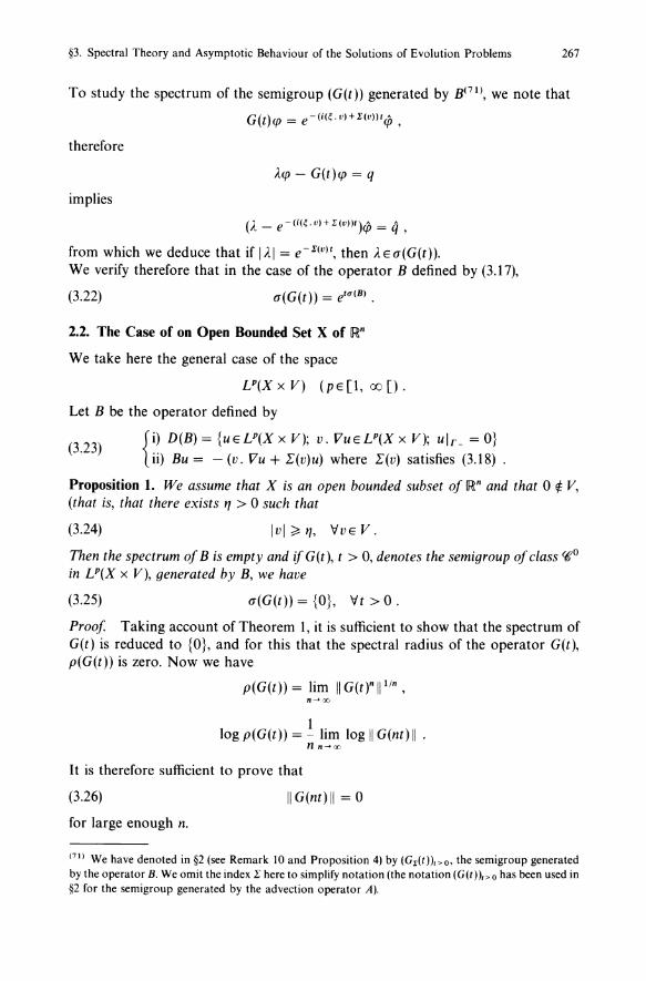
§3. Spectral Theory and Asymptotic Behaviour of the Solutions of Evolution Problems 267
To study the spectrum of the semigroup (G(t)) generated by B(7I), we note that
G(t)cp = e - (i(~. v) +I(V))t<p ,
therefore
ACP - G(t)cp = q
implies
(A - e-(i(~.v)+I(V))t)<p = q , from which we deduce that iflAI = e-I(V)t, then AE(J(G(t)). We verify therefore that in the case of the operator B defined by (3.17),
(3.22) (J(G(t)) = etu(B) .
2.2. The Case of on Open Bounded Set X of IRn
We take here the general case of the space
U(Xx V) (pE[l,oo[).
Let B be the operator defined by
(3.23) {i) D(B) = {UEU(XX V); v. VUEU(XX V); ulr_ =o} ii) Bu = - (v. Vu + l"(v)u) where l"(v) satisfies (3.18) .
Proposition 1. We assume that X is an open bounded subset of IRn and that 0 ¢ V, (that is, that there exists '1 > 0 such that
(3.24) Ivl ~ '1, VVE V.
Then the spectrum of B is empty and if G(t), t > 0, denotes the semigroup of class ~o in U(X x V), generated by B, we have
(3.25) (J(G(t)) = {a}, "It> 0 .
Proof Taking account of Theorem 1, it is sufficient to show that the spectrum of G(t) is reduced to {O}, and for this that the spectral radius of the operator G(t), p(G(t)) is zero. Now we have
p(G(t)) = lim II G(ttll lin, n- cx)
log p(G(t)) = ! lim log II G(nt) II . nn-oo
It is therefore sufficient to prove that
(3.26) II G(nt) II = 0
for large enough n.
(71) We have denoted in §2 (see Remark JO and Proposition 4) by (Gx(t)),>o, the semigroup generated by the operator B. We omit the index:r here to simplify notation (the notation (G(t)Lo has been used in §2 for the semi group generated by the advection operator A).
268 Chapter XXI. Transport
Now (see (2.51)), we have for all UoEU(X x V):
(3.27) G(t) uo)(x, v) = {uo(X - vt: v) exp( - l.'(v)t) if t ~ t(x, v) , o otherwise .
Since X is bounded, hypothesis (3.24) implies that there exists TO > 0 such that
t(x, v) ~ To, If(x, V)EX X V.
We deduce that
G(t)uo = 0 ,
for t ~ To, which establishes (3.26). D
In the converse case, where the set of velocities V contains a ball with centre 0 and radius '1, we see that the value of l.'(v) at the point v = 0 plays an essential role.
Proposition 2. We assume that X is an open bounded subset of ~n, that V contains a ball with centre 0, andfurther thatfor 1.' (besides (3.18)) there exists '1 > 0 such that for Ivl < '1, we have
1.'(0) ~ l.'(v) (72) •
Then the spectrum of the operator B defined by (3.23) in U(X x V), satisfies
(3.28) a(B)c{zEIC;Rez~ -1.'(0)},
and that of the semigroup G(t), t ~ 0 of class rcO in U(X x V) generated by B
(3.29) a(G(t)) c {zEIC; Izl ~ e-tI(O)} .
Proof First of all we prove the inclusion (3.29). Let A E IC and 8 > 0 be such that
ReA> - 1.'(0) + 8 .
We verify that the operator etA. - G(t) is invertible, or equivalently, that the operator 1- e-o'G(t) is invertible. It is sufficient to prove that the operator e-tA.G(t) has norm strictly less than 1. Since X is bounded, 1f'1 > 0 there exists T~ > 0 such that
Ivl>'1= >x-tvfj:X fort>T~.
We have, for all u E U(X x V)
-tA.G() ( ) {exp( - tl.'(v) - tA)u(x - vt, v) if t ~ t(x, v) e tux, v = o otherwise
and consequently
e-tAG(t)u(x, v) = e-t(HI(v»Go(t)u(x, v)
where (Go(t)) is the semigroup generated by the operator A = - v. V. Let '1 > 0 be
(72) This is a local minimum. We further assume (for simplicity) that ~ is regular at 0 (for example continuous).
§3. Spectral Theory and Asymptotic Behaviour of the Solutions of Evolution Problems 269
fixed and t > Tq • For Ivl > 1'/, we have x - vt ¢X and consequently (Go(t)u) (x, v) = O. We therefore have
(3.30) e-o'G(t)u(x, v) = exp( - teA. + 1"(v))) Y(I'/ -lvl)Go(t)u(x, v)
where Y is the Heaviside function (Y(O) = 1 if 0 > 0 and 0 otherwise). When Ivl < 1'/, we have 1"(v);?; 1"(0); we have
t(1"(v) + Re A.) ;?; £t
and (3.30) implies
Ile-o·G(t)ll.:s:: lexp( - teA. + 1"(v))IIIGo(t)ll.:s:: e- a < 1
which proves that etA ¢O"(G(t)), and also proves the inclusion (3.29). From Theorem 1, etA ¢ et<T(B), from which A. E O"(B) which establishes the inclusion (3.28). 0
Proposition 3. We make the assumptions of Proposition 2 with p = 2. We assume that the open set X is bounded and convex and that the function v --+ 1"(v) is twice contil1.uously differentiable in the ball of centre 0 radius 1]. We further assume that V = V, and that dJ.l = dv is the Lebesgue measure over V (or V). Then the inclusions (3.28) and (3.29) established in Proposition 2 are equalities and the spectra of Band G(t) are composed only of continuous spectra.
Proof If u E L 2 (X x V) is the solution of the problem
{ AU + v. Vu + 1"(v)u = 0 ,
ulr _ = 0 ,
then by using the method of characteristics, (see §2.4) we deduce that u = 0, and that the point spectrum of B is empty. Analogous reasoning for the adjoint B* shows that the point spectrum of B* and therefore the residual spectrum of Bare empty(73). To show that the continuous spectrum of B coincides with the half plane {zEIC: Rez.:s:: -1"(0)}, we shall prove that the operator AI - B, which is injective with dense image, is not invertible for ReA..:s:: - 1"(0). Taking account of the Banach isomorphism theorem, it is sufficient to show that there exists a family of functions U,j E D(B), b > 0, satisfying the relations
(3.31 ) {i) II u,jll ;?; C > 0 ,
ii) lim II A.u,j - BU,jII = 0 . .1-0
We introduce the set (IXw)wEsn - 1 of tangent planes to a sphere of radius R which is chosen large enough so that the sphere "contains" X. For given WESn - l , we have
IXw = {x E IRn; x . W = R} .
Every point x E X can be written uniquely in the form
x = Xo - SW,
(73) All this is also valid for P E ] 1, + 00 [ with only the hypotheses of Proposition 2.
270 Chapter XXI. Transport
where Xo E (xv) is the orthogonal projection of x over (xw and where s is a positive number between two values SI(XO, w) and sz(xo, w).
In particular for given v E V(v #- 0) and w = ~, the set L (v), where we impose the Ivl
boundary condition u = 0, is the set of points of the form
{x = Xo - sz(xo, w)w, XoEX w}
where Xw denotes the orthogonal projection of X over the plane ct.w' For every function u E L 2(X X V) the Fubini theorem gives (setting v = IUV):
(3.32) f lu(x,vWdXdv=fCDpn-IdPf Yv(pw)dw Xxv ° S"~1
f dxofS2lU(xo - SW, pwW ds (74)
Xw SI
Let b = inf sup (SZ(XO, W) - SI (XO, W))
weSn - 1 x oEX",
(since X is an open set, b > 0). We set
X~ = {xoEXw: Sz(xo, w) - SI(XO, w) ~ ~ b}; X:; is a subset of IXw with nonzero measure in lXV)' and there exists a constant C > ° such that we have
We introduce the function hb(P) which is equal to 1 on the interval [0, <5] and ° otherwise; <5 is chosen small enough so that
(3.33)
(This is realised, in particular, for <5:;;;; 11). We then set v = pw, WES n - 1 and
(3.34) _ hb(P)
Ub(X, v) = Ub(XO - sw, pw) = e(S st\(Hl'(O))/I'(sz - s) -----;;+t • <5-2-
We also set f3 = - ReA - l:(0)
(f3 is positive by hypothesis). For fixed w, S being defined by the relation
x = Xo - s(x, w)w , we have
(7") With Yv( J1w) = the characteristic function of V ( = 1 if J1W E V, 0 otherwise).
§3. Spectral Theory and Asymptotic Behaviour of the Solutions of Evolution Problems 271
from which
(3.35) v. VUb + (Je + 1:(V))Ub = ,ue(s-s!l(HI(O))/!l h bn(:,) + (1:(v) - 1:(O))Ub. b-z-
Now (3.32) and the definition of Ub (3.34) imply
1 fb f f iSZ S-So (3.36) II Ub Illz(x x V) ~ ~n + 1 ,un - 1 d,u dw. dxo (Sz - s)Z e - 2P-,- ds .
u 0 sn~1 X;, SI
3 Now, for Xo EX!, we have (S2 - sd ~ 4 b, and consequently
iSZ Zp is' +b/2 Zp (s - SZ)2 e -,,(S-S') ds ~ e-"(S-S')(s - Sz)2 ds SI 51
Further, noting that
iSZ ~ iSZ (S2 - sd3 (s-s2fe-'(S-s,)ds~ (s-szfds= 3 '
51 SI
we see that
f (S2 - Sd3 f X sn- ,dw(1:(,uw) - 1:(0))2 3 Xw dxo·
By applying the bound (3.33), we deduce
2 C3 fb n+3 _ C 3b3 11(1:(v)- 1:(O))Ub IILz(XxV)~ bn+ 1 o,u d,u - n + 4 .
Finally, we have
II ,u. e(s- s,) (H I(O))/!lh/;( ,u)jb n; , Illz(x x V)
272 Chapter XXI. Transport
2, (where we coarsely bound e -,(s-sd by 1). We deduce from (3.35) that
II (AI - B)u" II ~ CJ
which concludes the proof. o Remark 1. In the case where 1: is identically zero, the spectrum of A = - v. V,for X = IRn, is L2(X X V) is
a(A) = {ZEC; Rez = O} .
In the case of an open bounded subset X of IRn, if V does not contain the origin the conclusions of Proposition 1 are obvious. If V contains the origin, the conclusions of Proposition 3 hold by substituting 1:(0) = ° in (3.28) and (3.29). 0
3. Study of the Spectrum of the Transport Operator in an Open Bounded Set X of IRn
3.1. Perturbation Theorem
Let B be the operator defined in the preceding section by (3.23); we propose to study the spectrum of the transport operator
T= B+K
where K is the bounded integral operator called the collision operator, defined in (2.41) with the properties (2.40):
(3.37) (Kq>)(x, v) = Lf(x,V' ,V)q>(X'V' )dl1 (V ' ), XEX, VEV.
In agreement with the physical models, we assume in all of this §3 that we have J?: 0. Until now this property has not been useful for mathematical results(75). Now they will become essential, starting from §3.4, where we use the Krein~ Rutman theorems. Since we have characterised the spectrum of the semigroup generated by B in many situations, we shall obtain some more information on the semigroup generated by the operator B + K by using the following perturbation theorem, which obviously applies to an arbitrary operator B of U(X x V) which always has the property of being an infinitesimal generator of a semigroup of class rtl° in a Banach space.
Remark 2. The principal results on the spectrum of the operator T will be obtained from the spectrum of the operator Gdt) = etT by Theorem 1. 0
Theorem 2. Let B be the infinitesimal generator oj a semigroup oj class rtl°, G(t), t > 0, in a Banach space Z. Let, on the other hand, K be a bounded operator, and Gdt), t > 0, be the semigroup generated by the operator T = B + K.
(75) Except, obviously,for the positivity properties of the semigroup Gdt), t > 0 and of the solution u(t)
of the Cauchy problem for the given positive data Uo and q (see §2, Theorem 3 and Proposition 2).
§3. Spectral Theory and Asymptotic Behaviour of the Solutions of Evolution Problems 273
We assume that for t large enough, the operator
R(t) = t ds J: Gdr)KG(s - r)KG(t - s)dr
is compact. Then the part of the spectrum of the operator Gdt) contained in the exterior of the closed disk {z; Izl ~ e/W } (where w is the type of the semigroup {G(t) }<76») is formed at most from a countable sequence of eigenvalues of finite multiplicity, without a cluster point.
Remark 3. From Theorem 1, it follows that the part of the spectrum of the operator T = B + K situated in the band
{zEIC: w < Rez ~ Wd(77)
where Wl is the type of the semigroup {G l (t)}' and w, the type of {G(t)}, is only composed of a countable sequence of eigenvalues with finite multiplicity without an accumulation point. The operator B + K can therefore only have continuous spectrum in the half plane {Re z ~ w}. D
The proof of Theorem 2 relies on
Lemma 1. With the hypotheses and notation of Theorem 2, we have:
Gl(t) - G(t) = f~ Gl(s)KG(t - s)ds.
Proof of Lemma 1. Let ¢ E D(B) = D(B + K); we have
1/ d Gl (t)cp - G(t)cp = 0 ds (Gds) G(t - s)cp)ds
= t (Gds)(B + K)G(t - s) - Gds)BG(t - s)) cpds (78)
= t Gds)KG(t - s)cpds,
from which we have the result, since D(B) is dense in Z. D
Proof of Theorem 2. By applying Lemma 1 twice we can write
Gdt) - G(t) = f~ (f~ Gdr)KG(s - r)dr + G(S)) KG(t - s)ds ,
I (76) See Chap. XVII A, §1.2. Recall: the type w satisfies w = lim - log( II G(t) II).
1-00 t (77) We assume in this statement that w < w" which is not necessarily true under the conditions of Theorem 2 (thus K = 0 gives w = Wi).
d (78) We apply the property - G,<s)cf> = (8 + K) G,(s) cf> = G,(s)(8 + K )cf>.
ds
274 Chapter XXI. Transport
that is to say
G1(t) = G(t) + L G(s)KG(t - s)ds + fJ: G1(r)KG(s - r) KG(t - s)drds (79).
Let A E IC be given; we have
etA] - Gdt) = etA(I - e-tAG(t) - e- tA L G(s)KG(t - s)ds - e-O'R(t)).
Since {G(t)} is a semigroup of type w, for all E > 0, there exists ME such that
(3.38) IIG(t)ll:::;: Mtet(W+E).
Let AEIC with ReA > w. We shall choose E:::;: (ReA - w)/2. Let
We have
L(t, A) d~ e-tAG(t) + e- tA L G(s)KG(t - s)ds.
II L(t, A) II :::;: e-tRe(A)( MEet(W+E) + t ME211 K Ilet(w+E) dS) ,
:::;: et(-Re(A)+w+e)(ME + tME211K II),
:::;: e-tE(Me + tME211 K II) ,
which tends to zero as t --. (jJ. For t large enough we can make this as small as we wish (and in particular less than 1/2). We deduce that when ReA > w, the operator] - L(t, A) is invertible for t large enough. On the other hand, the function A --. (I - L(t, A))-l is holomorphic in the half-plane Re(A) ~ W + E.
Since
etA] - G1(t) = etA(I - L(t, 2) - e-AtR(t))
= etA(I - L(t, A))(] - e-A.t(I - L(t, A))-l R(t)) ,
we deduce that for the operator etA] - G1 (t) to be invertible, it is necessary and sufficient that the operator
] - e-At(I - L(t, ..1))-1 R(t)
is also. Since the operator R(t) is compact by hypothesis and the function
..1--. e - At(I - L(t, A)) - 1 R(t)
is holomorphic in the half-plane ReA > w we deduce from an "analytic Fredholm" theorem (see for ex. Kato [1], p. 370, Sanchez-Palencia [1], p. 315), that one of the
(79) This formula is usually called the second order Dyson-Phillips expansion.
*3. Spectral Theory and Asymptotic Behaviour of the Solutions of Evolution Problems 275
following situations is true: i) 1 is in the spectrum of e-lt(l- L(t, A))-t R(t) for all A; ii) I - e -It(l - L(t, A)) - t R(t) is invertible except for a family of numbers J1k without cluster points at finite distance in the half-plane w + G < ReA.. These points are eigenvalues with finite multiplicity. Since we have
II e-tl(l- L(t, A»-t II ::::.;; 2e- tReA ,
(using the bound II L(t, A) II ::::.;; 1/2), and letting ReA. tend to infinity, we deduce that only situation ii) holds true, from which we deduce Theorem 2, going back to the set
{zEIC; Z = etA, ReA. > w} . o
3.2. Application to the Transport Operator
To apply this theorem to the transport operator with the integral, that is to say to the operator T = B + K where B is the operator defined in (3.23), and K the integral operator defined in (3.37), we shall take the Hilbertian case where Z = H = L2(X x V)(80).
Proposition 4. We assume that X is an open subset to fRO which is bounded and convex, thauhe velocity space V is a closed subset of fRO with nonempty interior(8t), which V = V and with the Lebesgue measure dJ1 = dv, that 1: ~ 0 satisfies (3.18) and that the kernelf of the operator K does not depend on X(82\ satisfying (2.40), and that the function
w-+f'r (f(w,v)f(v',w»2dvdv', Jvxv
is locally integrable. Then the operator in L2(X x V)
(3.39) R(t) = Lt Gt(,r)KG(s - r)KG(t - s)drds, 'VtEfR+
is compact.
Proof By changing r to s - r, we write R(t) in the form
R(t) = f~ f~ Gds - r)KG(r)KG(t - s)dr ds .
(80) Indeed, we shall make use of the theory of Hilbert-Schmidt operators (see Chap. VI). (81) The results remains true if V is a finite union of concentric spheres (see Remark 4 with / = 1). (82) The result remains true if/depends on x, but also satisfies/Ix, v, v') <f(v, v') with/satisfying the same hypotheses as/(w, v) in Proposition 4.
276 Chapter XXI. Transport
Since the operators occurring in the integral are bounded, R(t) is bounded in norm(83) for '1 > 0, '1--+ 0, of the family of operators
R'1(t) = I J: GI(s - r)KG(r)KG(t - s)drds.
It is sufficient to prove that \1'1 > 0, R~(t} is compact. For this, it is sufficient to prove that for all (s, r) such that '1 ::::; r ::::; s ::::; t, the operator
Gds - r).KG(r).KG(t - s)
is a Hilbert-Schmidt operator and that its norm as a Hilbert-Schmidt operator is integrable over the triangle
T~ = {( s, r): '1 ::::; r ::::; s ::::; t} .
We know(84) that if AI, Az, A3 denote three bounded operators, it is sufficient that one of the three, for example A z, is a Hilbert-Schmidt operator for the product AIAzA3 to be, with, further,
We have
II GI (s - r) KG(r) KG(t - s) IIHs ::::; M; e(s-r)(w, +e) II KG(r)K IIHs. Mee(t-s)(w+e)
where we apply (3.38) and the inequality
(which is analogous to (3.38) for Gdt) whose type is therefore WI). We deduce (for WI > W)(85) that
It remains to show that the operator KG(r)K is Hilbert-Schmidt and to evaluate II KG(r)K IIHs. Now if q == G(r)Ku, we have, from (3.27), (3.37),
q(x, v) = Yx(x - vr)exp( - I"(v)r) tf(V', v)u(x - vr, v')dv'
where Y x(x) = 1 if x E X, = ° otherwise, denotes the characteristic function of the
(83) That is to say that IIR.(t) - R(t)1I ~ IIR.(t) - R(t)II.5I"(H.H)--+ 0 as '1--+ 0 for H = Z = L2(X X V).
(84) See Chap. VI. (85) Otherwise we replace WI by Wo = max(w, w,).
§3. Spectral Theory and Asymptotic Behaviour of the Solutions of Evolution Problems 277
open set X. We then have
(KG(r) Ku)(x, v) = Lf(V'" v)q(x, v")dv"
= Lf(V'" v) Yx(x - v"r)exp( - E(v")r)
x Lf(V" v")u(x - v"r, v')dv' dv" .
Setting x" = x - rv", we obtain (noting that dx" = r"dv"),
(KG(r)Ku)(x, v) = ~ L Ix Yve ~ x")f( x ~ x", v )f(V" x ~ X")
.exp ( - E(x ~ x")r)u(x'" v')dx"dv' .
The kernel of the KG(r)K operator is therefore the function
1 (x - x" ) ( x - X") (x - X") ( (x - X") ) -;nf -r-' v f v', -r- Yv -r- exp - E --r- r
and its Hilbert-Schmidt norm is bounded by the integral
IIKG(r)KII~s ~ r~" f iXXV)2 Yv(x ~ x")(I(x ~ x", v)y (I(v" x ~ x")y
dx dx" dv' dv .
Let K(r) be the closure of the set of points w of the form (x - x")jr with XEX, x" EX and '1 ~ r ~ t; K(r) is contained in a compact subset of [R", and since the function
w-+f'l (f(w,v)f(v',w))2dvdv' Jvxv
is, by hypothesis, locally integrable, we prove that the operator KG(r)K is a Hilbert-Schmidt operator, from which we deduce that R~(t) is also a Hilbert-Schmidt operator and we have the result. 0
Remark 4. In the case where the velocity space reduces to the sphere in [R3(86)
with centre 0 and radius ro = I v I = 1, with the surface measure (this model was seen in Chap. I, §5 and called the monokinetic model, the neutrons are assumed to have the same modulus of velocity vo), we have, assuming thatf = 1 and E constant for simplicity
KG(r) Ku(x, w) == f dw" Yx(x - w"r)e- Ir f u(x - w"r, w')dw' . S2 S2
(86) Here, n = 3.
278 Chapter XXI. Transport
We deduce by setting x" = x - w"r,
It f -Xlx-x"l f KG(r)Ku(x, w)dr = Y(t - Ix - x"l) e "12 u(x", w')dw' dx" ,
o x Ix - X S2
which again defines a compact operator. o Definition 1. We say that a collision kernelf(occurring informula (3.37) withf~ 0) satisfies the H.S.(87) hypothesis if we have
(3.40) f dw f'r (f(x, w, v)f(x, v', W»2 dv dv' ~ qK) R Jvxv
for all compact sets K of [R", where qK) is a finite positive constant which is independent of x and only depends on K. Example 2. If V is bounded, then the kernel defined by f(v', v) = fo where fo is a constant independent of v' and of v (which is a particular case of isotropic diffusion), satisfies the H.S. hypothesis. In this case, f satisfies the conditions of Theorem 2. 0
Example 3. We assume V = [R3 with the Lebesgue measure and that the kernel f satisfies the bound
(3.41 ) f( ' ) ~ __ c_ -a2Iv'-t'1 2j2 v,v"l 'Ie , v-v
then the H.S. hypothesis is satisfied. Indeed, we have
f-dw f (f(w, V»2 (f(v', W»2 dv dv' K VxV
~ 2 f d (I 1 -a2Iv-wI 2 -a2Iv'-wI2d d ') "c w ze ze v v K v x v I v - w I I v' - wi
~ c2 f dW( r _1_e-a2IvI2 dV)2 ~ c2 4rr3 meas(K) " K Jvlvl2 "a2 '
from which we have the stated result. (This example corresponds in neutron physics to an application where the nuclei which strike the neutrons are the atomic nuclei of a gas of free atoms)(88). 0
Applying Proposition 1, Theorem 2 and Proposition 4, we obtain
Theorem 3. (Jorgens). We assume that X is an open bounded convex subset of [R"
and that 0 tj V(89). We assume that the given positive data L does not depend on x and
(87) H.S. for Hilbert-Schmidt. (88) See Montagnini-Demuru [1]. _ (89) And further (Proposition 4) V = Vand dll = dv, or also V is a union of concentric spheres with centre 0 and dll the surface measure.
§3. Spectral Theory and Asymptotic Behaviour of the Solutions of Evolution Problems 279
satisfies 1: E L 00 (V) and that in addition to the inequalities (2.40), the collision nucleus f satisfies the B.S. hypothesis. Then the spectrum 0"( T) of the transport operator T defined by
(3.42) {i) D(T) = {uEL2(X X V); v. VUEL2(X x V), ulr_ = O} , ii) Tu = - v. Vu - 1:u + Ku,
is composed at most of a sequence of eigenvalues of finite multiplicity, bounded to the right, without a cluster point. The spectrum of the operator G1 (t) of the semigroup generated by T is, for all t composed at most of a sequence of eigenvalues of finite multiplicity without a cluster point other than O.
In the opposite case where 0 E V, Proposition 2, Theorem 2 and Proposition 4 imply
Theorem 4. We assume that X is bounded and convex and that V = V contains a neighbourhood of 0, with the Lebesgue measure over V. We make the same hypotheses over 1: and the collision nucleus f as in Propositions 2 and 4(90).
Then, the spectrum of the transport operator T is composed outside of the half-plane {z E IC: Re Z ~ - 1:(0)} (where there is a continuous spectrum) at most of a sequence of eigenvalues bounded to the right with finite multiplicity without a cluster point in the set
{Z;ZEC, - 1:(0) < Rez ~ - 1:* + II K II}
where 1: * = inf ess 1: ( V). VEV
The spectrum of the operator G1 (t) of the semigroup generated by Tis composed,for all t > 0, of a continuous spectrum in the disc {z; I Z I ~ e - tE(O)} and a countable set of eigenvalues with finite multiplicity in the ring
{z;e-tE(O) < Izi ~ et(-E'+IIKID} .
Proof Taking account of Proposition 2, of Theorem 1 and of Proposition 4, it only remains to show that the type of the semigroup {G 1 (t)} is less than - 1:* + II K II. Now if B again denotes the operator defined by (3.23) we have
Re(Bu,u)~ -1:*lluI1 2 •
We deduce immediately that
Re(Tu, u) ~ (- 1:* + II K II) II u 11 2 ,
from which we have the result(91). o
(90) That is to say: J: satisfies (3.18), has a local minimum at 0 and J satisfies the H.S. hypothesis (3.40). Therefore the hypotheses made in Theorems 3 and 4 on J: and J coincide outside of a ball 8,(0) c V. (91) Indeed T + J:* - II K II is then the dissipative infinitesimal generator of a semi-group, which is a contraction semigroup. Hence,
IletlTH'-IIKID II,,; 1, Ile'T II,,; e'l-r'+IIKII) ,
and the stated result follows.
280 Chapter XXI. Transport
Conversely, we can ask if the spectrum of T contains the half plane {z: Re z ~ - 17(O)} and the spectrum of Gt(t) the whole disc {z: Izl ~ e-tE(O)}. We can confirm this in the following particular case.
Theorem 5. We assume that n = 3 and that X is an open, bounded convex set, that the velocity space is equal to [R3(92), and that 17 and f satisfy the hypotheses of Theorem 4. We further assume that the collision nucleus f satisfies the bound
(3.43) , C -alvl 2 , f(x, v, v) ~ ~e ,Vv, v E V, VXEX.
We again denote by T the transport operator defined in H = L 2(X X V) by
(3.44) Tu = - v. Vu - .[(v)u + Ku
with absorbing boundary conditions, let u Ir _ = 0 and therefore
(3.45) D(T)= {UEe(XX V);v. VUEL2(XX V),uir- =O}.
Then the spectrum of the operator T contains the half-plane
{z; Re z ~ - '[(O)}
and the spectrum of Gdt) contains the disc
{z;lzl ~ e-tE(O)} .
Proof It is sufficient to show (see (3.31» that the function U,j defined in (3.34) satisfies II KUb II -+ 0 as b -+ O. Indeed, in this case, we have IIAu,j - Buo - Ku,j II -+ 0 as b -+ O. We have, with C denoting various constants,
I (Kuo)(x, vW = 1 Ivf(X, v', v)u,j(x, v')dv' 12 ~ 1 C Iv ~v-I~I::~ uo(x, v')dv' 12 ,
thus, setting v = JiW and v' = Ji' w' with w, w' E S 2 and Ji, Ji' E [R + :
1 (Kuo)(x, JiW) 12 ~ 1 C fO (Ji')2 dJ1' f dw' e -a:2 uo(x, w' Ji') 12
o S2 JiJi
(92) With the Lebesgue measure.
§3. Spectral Theory and Asymptotic Behaviour of the Solutions of Evolution Problems 281
We deduce
II KU61Ii2(xxv) ~ C(j3 f dx roo e- 2a1J2 djt f dw r6 djt'l u6(x,w'jt')1 2dw' x Jo S2 Jo
that is to say, using (3.34) (with n = 3) and the notation of the proof of Proposition 3,
C'ili f f lS~ (S-S'd) II KU611 i2(X x V) ~ T djt' 2 dw' dxo, (S2 - S)2 e - 2fJ -IJ-' ds. o s x.' s,
Now
( , _ )2 -2fJ -, d ~ C"!!:.... 1 _ -2fJ -, ~ C"!!:.... lS~ (s -s'd) , ( (s, - s', ) ) , sj s 2 s e IJ s '" 2fJ e I' '" 2fJ
implies
D
Remark 5. If f no longer models collisions between neutrons and atomic nuclei, but collisions between gas molecules in the framework of the linearised Boltzmann equation, the bound (3.34) is valid in the case where the molecules are "spherical balls" (the case of a monoatomic gas) (see Albertoni-Montagnini [1]). D
Remark 6. If we study the case where X is an open bounded convex subset of Illn
(with n not necessarily equal to 3) and where V is a bounded subset of Illn contained in a neighbourhood of the origin andfELOO(X x Vx V), the hypothesis (3.43) is a forteriori satisfied in the same way as (2.40) and (3.40)). The results of Theorem 5 also apply here, if f also satisfies the hypothesis of Theorem 4. D
Proposition 5. We assume that X is an open bounded, convex subset of 111 3 that V = Vis radial(93) with OE V, and with djt = dv, that 1: satisfies (3.18) and that the collision nucleus f is independent of x, and in addition to (2.40) satisfies the following hypothesis(94): there exists a function j from III + x III + -+ III + such that
If(v,v')I~j(lvl,lv'I), VV,V'EV
(93) That is to say invariant by rotation around the centre O.
(94) Proposition 5 is proved for fnot depending on x. It remains true iff, depending on x, is bounded by a function f. independent of x satisfying the hypotheses of the proposition.
282 Chapter XXI. Transport
and constants C1 , C2 , C3 (strictly positive) such that
(3.46) Loo pi J(pl, p) dp ~ C 1 , VP'EIR+ ,
(3.47) Loo p'l(pl, p)dp' ~ C2 , VPE IR+ ,
(3.48) 1'(v) ~ 1'(0) - C3 1 vi, VVE V.
Then the transport operator has no eigenvalue in the half-plane {z E C: Re z > - 1'(0)}, if the diameter of the open set X is small enough.
Remark 7. Inequalities (3.46) and (3.47) are conditions of decreasing at infinity for the collision kernel f, which are pointless if the space V of velocities is bounded. Hypothesis (3.48) is (from hypothesis (3.l8)) a local hypothesis on the behaviour of l' at 0 (the graph of l' is above a cone at the neighbourhood of 0, and 0 is not necessarily a local minimum of 1'). With the additional hypotheses of Theorem 4, that is, if
{ i) l' has a local minimum at 0 (which implies (3.48)) and
ii) f satisfies the H.S. hypothesis (3.40),
then O'(T) c {z E C: Re z ~ - 1'(0)}, if the diameter of X is small enough; further if l' is regular at 0 (see Proposition 3), the inclusion is replaced by equality. 0
Proof of Proposition 5. We prove that if Re A > - 1'(0), then the equation
which is equivalent to
Tu = AU,
{ AU + v. Vu + 1'(v)u - Ku = 0
ulr _ = 0
does not possess a solution other than u = 0 in L 2(X x V). We set (denoting by YIV1(P) the characteristic function of the set IV I ~ {I v I, v E V} c IR + )
cp(x,p)=p ylV,(p)f lu(x,wp)ldw. S2
By using the method of characteristics(95), we see that
ft(x.V)
u(x, v) = Jo exp( - (1'(v) + A)t)(Ku)(x - vt;v)dt
(95) See for example the proof of Proposition 6 of §2.
§3. Spectral Theory and Asymptotic Behaviour of the Solutions of Evolution Problems 283
where t(x, v) denotes the exit time. By noticing that
1 t(x, pw) = - t(x, w)
P
and by setting s = pt, we find
1 rt(x.W) ( s) u(x, pw) = p Jo exp - (I'(wp) + A) P (Ku)(x - wS,wp)ds
= t f~(x,W) exp ( - (I'(wp) + A) ~) L!(V', wp)u(x - ws, v')dv' ds .
We then obtain
1 rt(x.W) ( s) f -lu(x,pw)l~pJo exp -(I'(pw)+ReA)p v!(lv'l,p)lu(x-ws,v')ldv'ds
~ t rx,W
) exp ( - (I'(pw) + ReA) ~)
f~ p'2 J(p', p) Ywl(p')dp' fS21 u(x - ws, w'p')1 dw' ds
from which (here with pEl VI)
<p(x, p) ~ L2 dw f~(x,W) exp ( - (I' (pw) + ReA) ~)
x Loo p'l(p', p)<p(x - ws, p') dp' ds .
Setting x' = x - ws and noting that
f f t(x.W) f ljJ(x', I x - x'l) , dw ljJ(x - ws, s) == '1 2 dx,
S2 0 X Ix - x
we obtain (with w = (x - x')/I x - x'l)
f 1 ( I x - x' I) roo -<p(x, p) ~ x dx' I x _ x' 12 exp - (I'(pw) + ReA) p Jo p'!(p', p)<p(x', p') dp';
and noting that from inequality (3,48)
lexp ( - (I'(pw) + A) ~) I ~ exp ( - (I'(O) + ReA) ~ )exP(C3s)
~ exp(C3s),
then since ReA + I'(O) ~ 0,
f eXP(C3(X-X'l) loo-<p(x,p)~ dx' I '1 2 p'!(p',p)<p(x',p')dp',
x x - x 0
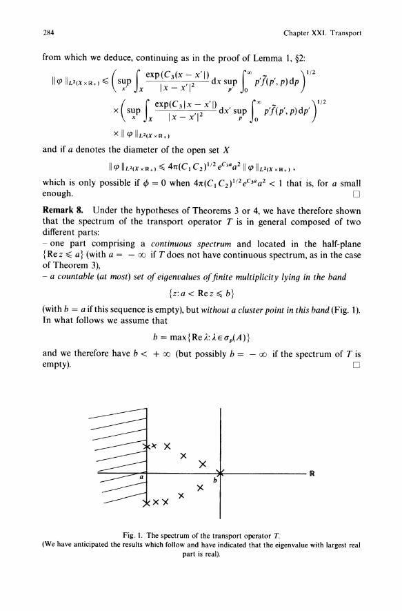
284 Chapter XXI. Transport
from which we deduce, continuing as in the proof of Lemma 1, §2:
( f exp(C3(x-x'l) 100 - )1/2 IIIP IIL2(Xd+) ~ sup I '12 dx sup p'f(p', p)dp
x' x x - x p' 0
( f exp(C3lx - x'l)d' fOO ',/-(' )d ,)1/2 x sup I '12 X sup P p, P P
x X x-x p 0
x IIIP IIL2(xx~+) and if a denotes the diameter of the open set X
IIIP IIL2(x x R+) ~ 47t(C 1 C 2)1/2 eC 'Qa2 IIIP II L2(X x ~+) , which is only possible if 4J = 0 when 47t(C1 C2 )1/2eC'Q a 2 < 1 that is, for a small enough. 0
Remark 8. Under the hypotheses of Theorems 3 or 4, we have therefore shown that the spectrum of the transport operator T is in general composed of two different parts: - one part comprising a continuous spectrum and located in the half-plane {Re z ~ a} (with a = - 00 if T does not have continuous spectrum, as in the case of Theorem 3), - a countable (at most) set of eigenvalues of finite multiplicity lying in the band
{z:a<Rez~b}
(with b = a ifthis sequence is empty), but without a cluster point in this band (Fig. 1). In what follows we assume that
b = max{Rd:A.EO"p(A)}
and we therefore have b < + 00 (but possibly b = - 00 if the spectrum of T is empty). 0
x X X
)< R
b )(
x)( )(
Fig. 1. The spectrum of the transport operator T. (We have anticipated the results which follow and have indicated that the eigenvalue with largest real
part is real).
§3. Spectral Theory and Asymptotic Behaviour of the Solutions of Evolution Problems 285
Remark 9. We can also apply Theorems 2, 3, and 4 (under the hypotheses) to the adjoint T* of the transport operator T. We deduce(96) that T* has continuous spectrum in the half-plane {Re z ~ a} and has eigenvalues of finite multiplicity in the band {a < Rez ~ b}, where the quantities a and b are the same as in Remark 8. Since neither Tnor T* has residual spectrum (under the preceding hypotheses), we deduce that if A is an eigenvalue of T then I is an eigenvalue of T*(97). In certain particular cases (see later Sect. 5), we can show that the eigenvalues are real. We show later (see Remark 17) that the spectrum 0'( T), and also the point, continuous and residual spectra of T are symmetric with respect to the real axis, which implies that these spectra are identical to those of the operator T*. 0
Remark 10. Intuitive interpretation of the difference between the spectra of T in Theorems 3 and 4. Let us consider the problem
(3.49) J~~ = Tu
1 u(O) = uo
in the case of the operator T of Theorem 3, then that of Theorem 4. In the two cases the open set X is bounded. In the first case (Theorem 3), the modulus of the velocity is bounded from below by Vo > O. After a transitory regime, the initial particles will all have disappeared (either by leaving the domain X or by absorption or by being deflected). The semigroup (G 1 (t)) generated by Tis compact for t large enough(98), and the operator T only has a point spectrum. In the second case (Theorem 4), the neutron velocities can be, on the other hand, very small and if the mean free path is smaller less than the domain X, at every instant t > 0, there will be some "initial" particles which will not leave X. The transitory regime mentioned above will never end and there is no chance of entering a "mode regime". 0
4. Positivity Properties
For simplicity we restrict ourselves here to the Hilbertian framework and we only consider the theory in the space H = L 2(X X V). We shall be interested in the eigenvalue with largest modulus of the semigroup (Gdt)) generated by the transport operator T, and with the eigenvalue with the largest real part of the transport
(96) Note that this follows directly from the fact that the spectrum of T* can be deduced from the spectrum of T by symmetry with respect to the real axis (see for example Kato [1], p 184). (97) This also follows from the following property (see Kato [1], p. 184): if A is an isolated eigenvalue of the operator T, then X is an isolated eigenvalue of T* with the same multiplicity. (98) Indeed, from the proof of Theorem 2, the operator
G,(t) - G(t) - f G(s)KG(t - s)ds
is compact; by taking t > 2to with to ~ supt (x, v), we obtain that G, (t) is compact. x.v
286 Chapter XXI. Transport
operator T. These eigenvalues and "the" eigenfunction with which they are associated have a very particular importance in applications (see (3.15) and (3.16». We shall show with the help of the Krein-Rutman theorem that these eigenvalues are simple, and that they correspond to a positive eigenvector. We have seen in §2 that the transport semigroup (Gdt)bo preserves positivity (Proposition 2 of §2) and therefore that the solution of the Cauchy problem (2.44) is positive for given data Uo and q which are positive (see Theorem 3 of §2). Likewise the solution of the stationary equation
(3.50) Au-Tu=q (AEIR,q>O)
is positive for large enough A( A > Ao). In the framework of the theory of matrices, the Perron-Frobenius theorem (see Chap. XX) allows us to confirm that under the properties of "positivity" a matrix has one of its eigenvalues equal to its spectral radius (therefore positive). This theorem was generalised to the case of infinite-dimensional linear operators by Krein-Rutman:
The Krein-Rutman Theorem(99). Let K be a compact operator in LP(Q)(lOO),
p E [1, + 00] such that u ~ 0 implies that Ku ~ O. If p(K) is the spectral radius of K, assumed nonzero, then p(K) is equal to an eigenvalue of K. This eigenvalue corresponds to a nonnegative eigenvector Up(K) with
(3.51 ) KUp(K) = p(K)Up(K), Up(K) ~ 0 and Up(K) #- 0 .
In the case where the operator is not compact we have:
The Krein-Rutman-Schaefer Theorem. Let R be a bounded operator in LP(Q)(lOI),
pE [1, + 00] such that U ~ 0 implies Ru ~ O. Then p(R)Ea(R)(where p(R) is the spectral radius of R) and if p(R) is a pole of the resolvent then its order is maximal on the circle of radius p(R). Therefore if p(R) is an eigenvalue with finite multiplicity m, every element of a(R) on the circle of radius p(R) can only be an eigenvalue of multiplicity ~ m. We then verify (see Schaefer [1], p. 266) that there exists a positive eigenvector associated with p(R). We have:
Theorem 6. We assume the conditions of Theorems 3 or 4. We again assume that the collision nucleus f is positive (f ~ 0) and, further, that the transport operator T has eigenvalues of finite multiplicity in the band
{a < Rez ~ b} (102)
(99) See Chap. VIII, Appendix "Krein-Rutman Theorem". (100) With Q a locally compact space equipped with a positive Radon measure jl; this theorem is more generally valid for every (real) Banach space with a reproducing convex cone (see Appendix of Chap. VIII). (101) Or more generally if E is a (real) Banach space with a reproducing convex cone (see Appendix of Chap. VIII). (102) (With b > a; see the notation of Remark 8).
§3. Spectral Theory and Asymptotic Behaviour of the Solutions of Evolution Problems 287
We set
(3.52) A(T)= sup {Rez}. ZE<7(T)
Then A (T) is an eigenvalue with at least one corresponding positive eigenvector. We shan call this eigenvalue the principle eigenvalue.
Lemma 2. Let Z be a Banach space and T an unbounded operator in Z, with domain D(T). Let Ra be the operator Ra = (aI - T) - I, where a E IC is a given scalar, a ¢ (J( T); then
(J(Ra) = {J1EIC: J1 = (a - A)-I, where AE(J(T)} u {O} .
Proof We shall show that if A ¢(J(T), A of- a, then J1 = (a - A)- J ¢(J(Ra) and that conversely, if J1 ¢ (J(Ra) then A ¢ (J( T). i) Assume therefore that A ¢(J( T), Ie of- a. The operator (AI - T) - I being continuous for all WE Z and for
(3.53) u ~ [(a - A)2(AI - T)- J + (a - A)I]w ,
we have
(3.53)' Ilull ~ Cllwll where C is a constant independent of w. Now (3.53) is equivalent to
that is to say
(AI - T)u = (a - A)«a - A)W + (AI - T)w)
= (rx - A)«aI - T)w)
(aI - T)u - (rx - ),)u = (a - A)(aI - T)w .
The operator aI - T being invertible by hypothesis, this is equivalent to
(a - A)-J U - (aI - T)-I u = w.
We therefore have proved that for all WE Z, the problem
(J1I - Ra)u = w ,
has a unique solution u satisfying (3.53)' from which J1 ¢ (J(R,). ii) Conversely, assume that J1 ¢(J(R,), J1 = (a - ),)-1, then for an WEZ and for
(3.54)
we again have the bound (3.53)' by hypothesis. From (3.54), we deduce that
(J1I - Ra)u = (rx - A)-I(cxI - T)-I w
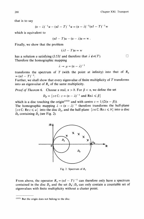
288 Chapter XXI. Transport
that is to say
which is equivalent to
(rxI - T)u - (rx - A)U = w .
Finally, we show that the problem
(AI - T)u = w
has a solution u satisfying (3.53)' and therefore that A ¢ 0"( T). Therefore the homographic mapping
A - J1 = (rx - A) - 1
o
transforms the spectrum of T (with the point at infinity) into that of Ra =(rxI_T)-l. Further, we shall show that every eigenvalue of finite multiplicity of T transforms into an eigenvalue of Ra of the same multiplicity.
Proof of Theorem 6. Choose rx real, rx > b. For f3 < rx, we define the set
D(J = {ZEC: Z = (rx - }.)-l and ReA ~ f3}
which is a disc touching the origin(103~ and with centre Z = 1/(2(rx - f3». The homographic mapping A _ (rx - A)-l therefore transforms the half-plane {z E C: Re Z ~ a} into the disc D a' and the half-plane {z E C: Re Z ~ b} into a disc Db containing Da (see Fig. 2).
ilR
)(. )(. X
A.o 0
Db
Fig. 2. Spectrum of R"
From above, the operator Ra = ('XI - T)-l can therefore only have a spectrum contained in the disc Da and the set Db \Da can only contain a countable set of eigenvalues with finite multiplicity without a cluster point.
(103) But the origin does not belong to the disc.
§3. Spectral Theory and Asymptotic Behaviour of the Solutions of Evolution Problems 289
On the other hand, the operator Ra leaves the cone of positive functions of U(X x V) invariant. (In effect we have
Ra = Loo e-atGdt)dt,
where (G 1 (t)) is the semigroup generated by the transport operator T, which leaves the cone of positive functions invariant). From the Krein-Rutman-Schaefer theorem (and the hypotheses made), if J.1.0 denotes the eigenvalue of Ra with largest modulus, then J.1.0 is real with J.1. > 0 and it corresponds to a positive eigenfunction Wo.
We call ..1.0 the reciprocal image of J.1.0 under the homographic mapping A f---+ (IX - A)-I; ..1.0 is real and from Lemma 2 it is the point on the spectrum which is closest to IX.
Therefore there does not exist another eigenvalue of T in the disc of centre IX with radius IX - ..1.0 ,
To show that ..1.0 is the eigenvalue of T with largest real part, we reason by contradiction: if Thas an eigenvalue Al satisfying Re Al > Re ..1.0 , we reach a contradiction by choosing IX large enough so that the disc of centre IX and radius IX - ..1.0
contains AI' On the other hand, we have
(IXI - T)-l wo = (IX - Ao)-IWo
and the function o ~ (I T)-1 u - IX - Wo
(which is positive) satisfies
that is to say Tuo = Aouo .
We have therefore shown that there is a positive eigenfunction corresponding to ..1.0 ,
Therefore with the notation of Theorem 6 (see (3.53)), ..1.0 = A( T) is the principal eigenvalue of T. 0
We shall now make an additional hypothesis to prove that this eigenvalue is simple. The hypotheses of Theorem 6 do not allow us to confirm that A (T) is a simple eigenvalue, nor that there exist other eigenvalues with the same real part. Conversely, if we assume, further, that the collision nucleus f(x, v, Vi) is strictly positive (f> 0) on X x V x V, we have
Theorem 7. We assume the conditions of Theorem 6. We assume too that the collision nucleus f is a "strictly positive" function, i.e. f ~ C > 0, C constant, and that the velocity space V contains a torus of the form
Vo = {VEIR3: ao ~ Ivl ~ al} (104)(105)(106).
(104) The result remains true if V is a finite union of spheres centred at O. (105) The calculation is identical in W. (106) It is sufficient thatfis "strictly positive" over the set (X x Vo x V) u (X x Vx VoJ.
290 Chapter XXI. Transport
Then the eigenvalue of T with largest real part is real and simple; we can associate a strictly positive eigenfunction with it(107). Further, there is no other eigenfunction associated with another eigenvalue, with constant sign.
Remark 11. i) Assume instead of the hypothesis of Theorem 7 that the functionf( = f(x, v', v)) has the following property: there exist Vt and V2 closed and disjoint, with nonzero measure for the measure Ji, with V = Vt u V2 and
{ f(X,V',V)=O, VXEX, VV'EVt , VVEV2 and VXEX, VV'EV2 , VVEVt
With the obvious notation:
U(X x V) = U(X x VdEB U(X x V2)
and the transport operator T in X x V decomposes into two operators T t over Xx VI and T2 over Xx V2: T= TtEBT~108), or that O"(t) = O"(Tdu 0"(T2)(108). Such a situation allows us to obtain easily some examples where the eigenvalue with largest real part is not simple. We therefore see that the conclusions of Theorem 7 are directly linked to the impossibility of such a decomposition. For further expansion on these relations, we refer to Voigt [1]. ii) We cannot apply the strong Krein-Rutman theorem here (see Appendix of Chap. VIII) to demonstrate Theorem 7, since the cone of positive functions of the space U(X x V), P E [1, + CI) [, has empty interior. We shall prove Theorem 7 with the help of a strictly positive kernel. D
Proof of Theorem 7. i) The positive eigenfunction indicated in Theorem 6, denoted uO, is the solution of the equation (with Ao = A(T)):
Aouo + v. Vuo + L(V)UO = Kuo, with Kuo(x, v) = tf(V', v)UO(x, v')dv' .
To show that UO is strictly positive(109), it is sufficient to prove: qo(x, v) > 0 V(x, V)EX X V, where qo = KUO(llO). We have, in an equivalent way (with (3.23))
Aouo = Buo + Kuo
(107) Except on the boundary r _ where it is zero.
(108) Likewise, the transport semigroup (G , (t)) decomposes into (G~')(t)) and (G~2)(t)) respectively in X x V, and X x V2 , which expresses the fact that a neutron with initial velocity v E V, never reaches the velocity v E V2 and vice versa.
(109) Except on the boundary r_ where uOI,_ = o. (11 0) In effect we then have:
It(x.V)
uo(x, v) = ° exp( - (r(v) + ).)t)qo(x - vt, v)dt > 0,
except on r _ where uo = o.
§3. Spectral Theory and Asymptotic Behaviour of the Solutions of Evolution Problems 291
and
from which
that is to say
qo(x, v) = Iv dv'f(v', v) f~(X'v') dt e-I(AOH(v')) Ivf(V'" v,)uo(x - tv', v")dv
= [ f(v', v)f(v", v') [00 e-I(AoH(v')) Yx(x - tv')uo(x - tv', v")dtdv' dv" Jvxv Jo
where Yx is the characteristic function of the open set X. By setting x' = x - tv', we obtain
qo(x, v) = LxvI" dtexp ( -t(AO+17(X~X'))/3 Yv(X~X')
Xf( x ~ x' ,v )f( v", x ~ x') uO(x', v")dx' dv" .
The hypothesis made over the velocity space V shows that for
I x - x'i I x - x'i '-------' ~ t ~ , we have
al ao
We deduce that the kernel L given by
x - x' --EV.
t
'" [00 ( ( , (x - x')) 1 (x - x') L(x, v; x ,v ) = Jo exp - t ...1.0 + X -t- (3 Yv -t-
(X - x' ) ( x - x' ) xf -t-'V f v"'-t- dt
is strictly positive since f is strictly positive; since
qo(x, v) = f L(x, v; x', v")uo(x', v") dx' dv" xxv
and that Uo is positive and not identically zero, we deduce: qo(x, v) is strictly positive. ii) We recall that the adjoint operator of Tis the opertor T* = B* + K* where B* is defined by
B*u = v. Vu* - 17(v)u*
and the adjoint boundary conditions (see §2.4.3). The operator T* has some properties analogous to T. In particular (see Remark 9), under the hypotheses of Theorem 6, in the band a < Re z ~ b the operator T * has eigenvalues of finite mUltiplicity which are the conjugates of those of T.
292 Chapter XXI. Transport
Further, Ao is also the eigenvalue of T* with largest real part and it corresponds to an positive eigenfunction u*o likewise strictly positive(111) by repeating an analogous argument. We deduce that if AEa(T) is an eigenvalue with A =I- Ao and if u is the eigenfunction with which it is associated, then u cannot be of constant sign: in effect, we have
Tu = AU uED(T)
T*u*o = AoU*o u*oED(T*).
By scalar multiplication of the first equation by u*o, the second by u and subtracting, we obtain
0= (Tu, u*O) - (T*u*o, u) = A(U, u*O) - Ao(U*o, u)
= (A - AoHu, u*O)
and since A =I- Ao, we deduce that
(u, u*o) == f u(x, v)u*O(x, v)dxdv = 0 Xxv
so that u cannot be of constant sign. iii) Finally we show the simplicity of the principal eigenvalue Ao. Assume that is not the case, then there are two eigenfunctions of T corresponding to Ao, UO and wo which are linearly independent, and we can choose ex E IR such that 1/1 = UO + exwo does not have constant sign. By setting
w* = (Ao - B*)u*o = K*u*o
and by remarking that
we have
We also obtain
= (11/1 I, K*(Ao - B*)-1 K*(Ao - B*)-1 w*) = (11/1 I, w*) .
In fact, we shall show that
E1 < E2 ,
from which we have a contradiction.
(111) Except on the boundary r + where it is zero.
§3. Spectral Theory and Asymptotic Behaviour of the Solutions of Evolution Problems 293
To establish the preceding inequality we remark that the function
0.0 - B) - 1 K 0.0 - B) - 1 K II/! I - 0.0 - B) - 1 K 0.0 - B) - 1 K I/!
is strictly positive. In effect the function II/! I - I/! is positive and not identically zero by hypothesis, and since the operator K 0.0 - B) - 1 K has a strictly positive kernel (see above), the function
Ko.o - B)-l K(II/!I-I/!)
is strictly positive from which we have the result. o Remark 12. Theorem 7 shows that Ao is geometrically simple(112). We show that Ao is algebraically simple(113). Assume that there exists U E L 2(X X V) which is nonzero and j ~ 2 such that
0.0 - T)ju = 0 with 0.0 - T)j-l U # 0 ;
then, by setting u 1 = (Ao - T)j - 1 U and U2 = 0.0 - T)j - 2 u, we see that
0.0 - T)Ul = 0 ,
(Ao - T)U2 = Ul ;
since AO is geometrically simple from Theorem 7, we have Ul = uo. By taking the scalar product with u*o the strictly positive eigenfunction of T* (except on T+), we deduce
(UO, u*O) = (0.0 - T)U2' u*O) = (U2' 0.0 - T*)u*O) = 0 ;
which is impossible since Uo and u*o are strictly positive: we deduce that AO is algebraically simple. 0
Remark 13. Under the hypotheses of Theorem 7, the eigenvalue with largest real part is not only simple, but no other eigenvalue can have the same real part. For this consider the semigroup (G1(t)) generated by the operator Twhich leaves the cone of positive functions invariant. From the Krein-Rutman-Schaefer theorem and Theorem 1, the largest eigenvalue of G1 (t) is simply el).o which is the spectral radius of G1 (t). Assume that there exists bE IR such that AO + ib E a( T), then el().o + ib) E a( G dt)) with p(G1(t)) = e tAo (we say that el().o+ib) belongs to the peripheral spectrum of G1(t), denoted aper(Gdt)) for all t ~ 0). Consequently (see Schaefer [2], Chap. V, corollary of Theorem 4.9 and Voigt [1]), aper(Gdt)) is periodic for t > 0, therefore t(b/2n) is rational for all t > 0, from which we have b = O. By then applying the part of Theorem 1 relating to the point spectra we deduce the desired result. 0
(112) That is to say that the proper subspace ker 0'0 I - T) is of dimension 1. (113) That is to say that sup dim (ker (}.ol- T)k) = 1.
kEN'"
294 Chapter XXI. Transport
Proposition 6(114). We assume that the transport operator T has eigenvalues of finite multiplicity in the band
{ZEC;a < Rez ~ b}
with b > a, the remainder of the spectrum of T being situated in the half-plane {ZEe, Rez ~ a}(115); then the semigroup (Gdt)) associated with the transport operator T, behaves asymptotically as t -> + OCJ as el'\o where Ao is the eigenvalue of T with largest real part.
Remark 14. In the case where T has only a continuous spectrum (b = a), we only know that the type of (G 1 (t)) is equal to a, and therefore that for all c > a, there exists a constant Mc such that
o Proof of Proposition 6. From Remark 13, there exists c < Ao such that the spectrum of the operator T when we have removed Ao is inside the half plane {Rez ~ c}. Then let robe the circle of centre Ao and radius 0.0 - c )/2. Since Ao is algebraically simple the operator
- 1 f' -I d' Po = P,\o = -.- (Ie - T) Ie 2m: 1"0
is a projection operator over the one dimensional subspace associated with the eigenvalue Ao (see Theorem 7). The restriction of the operator T to the supplementary subspace (/ - Po)H with H = L2(X X V) (or more generally C(X x V)) is unbounded and its spectrum is contained in the half plane {Re z ~ c}. On the other hand, the semigroup (Gdt)), t > 0 commutes with Po, and the generator of the semigroup Gdt)I(I-Po)H, t > 0, is the operator TI(I-Po)H and the spectrum of G 1 (t) I (I - Po)H is contained in the disc {I z I < eCI }.
Therefore, the type of the semigroup Gdt) 1(1_ Po)1l is strictly less than c and there exists a constant Mc such that
II Gdt)I(1-Po)H II ~ Mc ecl.
Since
G1(t) = Gdt)Po + Gdt)(I - Po),
we deduce that (as t -> + OCJ )
Gdt) = Gdt)Po + O(eCI ) •
(114) This result coincides with that given for exp(tA) where A is a matrix in the introduction (in §3.1). As in this Proposition 6 we have an unbounded operator it is necessary for the proof: i) to analyse by a perturbation method the spectrum of the transport operator T in the band Re Z > a. ii) to prove that we have
a(eIT)n{ZEClzl>e-la}ce,"(Tl;
iii) to use the Krein-Rutman theorem. (115) In particular this will be true under the hypotheses of Theorems 3 and 4, see Remark 8.
§3. Spectral Theory and Asymptotic Behaviour of the Solutions of Evolution Problems 295
Now the proper subspace Po H of the operator G1 (t) reduces to a simple multiplicatIon by e'AO. We therefore have (for t --+ + 00)
Gdt) = e'AOpo + O(eCI )
from which we have the result since c < AO. o
Remark 15. By using "the" eigenfunction u*o of the adjoint operator T* associated with the eigenvalue Ao, introduced in the course of the proof of Theorem 7, we obtain a more explicit form of the projection operator Po:
(3.55)
if we assume that u*o and UO are normalized so that
(uo, u*O) = 1 . o
Remark 16. We often have the following situation in applications: we look for A(T), the principal eigenvalue of the problem: find uED(T) such that
(3.56) Tu=A(T)u.
If we have found an eigenfunction w of the problem
(3.57) Tw= AW
and if w satisfies w ~ 0 not identically zero, then it follows that the function u which we are seeking is
u = w.
Now, it may be simpler to firstly calculate the solution w of problem (3.57); in effect, if the problem (3.56) has symmetries, then u, linked to the principal eigenvalue, has the same symmetries. We shall then resolve (3.57) by looking for a solution with the desired symmetries. 0
Criticality. Under the hypotheses of Proposition 6 (and of Theorem 7), we can, referring to the introduction of this §3, give a precise definition of the criticality of the problem
(3.58) i·) du d 1 dt = Tu + q, q indepen ent of t
ii) u(O) = Uo, with Uo and q given in L 2(X x V).
1) The case where A(T), the principal eigenvalue of the operator T satisfies
(3.59)i) A(T) > 0 .
Then there exist Uo and q such that the solution of the evolution problem tends towards + 00 with t. Problem (3.58) is then called supercritical. 2) The case where A(T) satisfies
(3.59)ii) A(T)<O.
If q = 0 the solution of problem (3.58) tends to 0 as t --+ + 00 exponentially.
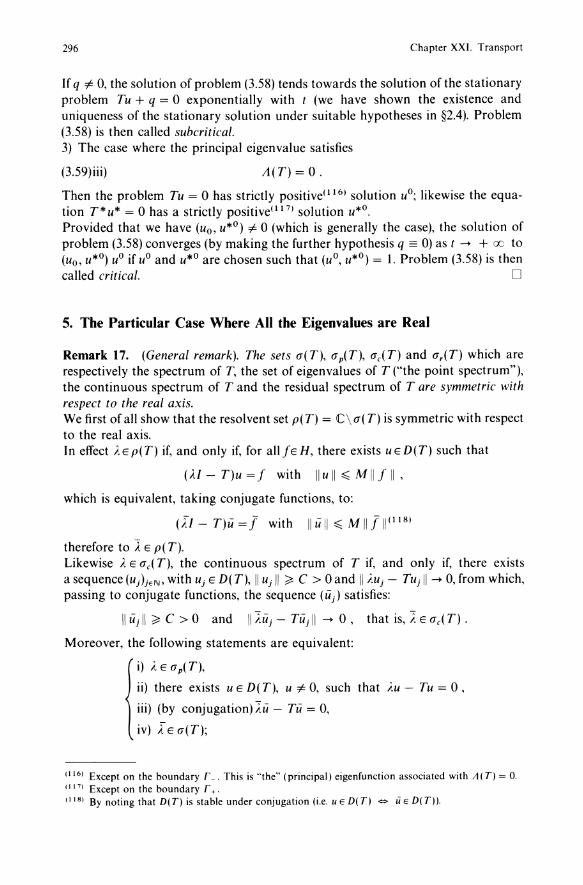
296 Chapter XXI. Transport
If q i= 0, the solution of problem (3.58) tends towards the solution of the stationary problem Tu + q = 0 exponentially with t (we have shown the existence and uniqueness of the stationary solution under suitable hypotheses in §2.4). Problem (3.58) is then called subcritical. 3) The case where the principal eigenvalue satisfies
(3.59)iii) A(T)=O.
Then the problem Tu = 0 has strictly positive(l16) solution uo; likewise the equation T*u* = 0 has a strictly positive(l17) solution u*o. Provided that we have (uo, u*o) i= 0 (which is generally the case), the solution of problem (3.58) converges (by making the further hypothesis q == 0) as t ....... + oc to (uo, u*o) Uo if Uo and u*o are chosen such that (uo, u*o) = 1. Problem (3.58) is then called critical. D
5. The Particular Case Where All the Eigenvalues are Real
Remark 17. (General remark). The sets (J(T), (Jp(T), (Je(T) and (J,(T) which are respectively the spectrum of T, the set of eigenvalues of T ("the point spectrum"), the continuous spectrum of T and the residual spectrum of T are symmetric with respect to the real axis. We first of all show that the resolvent set p(T) = iC\(J(T) is symmetric with respect to the real axis. In effect A E p(T) if, and only if, for all IE H, there exists u E D( T) such that
(AI - T)u = I with II U II ~ M II I II ,
which is equivalent, taking conjugate functions, to:
(II - T)u = 1 with II u II ~ M 11.111(118)
therefore to ~ E p( T). Likewise Ie E (Je( T), the continuous spectrum of T if, and only if, there exists a sequence (Uj)jEII" with Uj E D( T), II Uj II ~ C > 0 and Ill.uj - TUj II ....... 0, from which, passing to conjugate functions, the sequence (Uj) satisfies:
II Uj II ~ C > 0 and II AUj - TUj II ....... 0, that is, A E (Je( T) .
Moreover, the following statements are equivalent:
i) Ie E (J p( T),
ii) there exists U E D( T), u i= 0, such that i.u - Tu = 0 ,
iii) (by conjugation) AU - Tu = 0,
iv) IE (J(T);
(116) Except on the boundary r _. This is "the" (principal) eigenfunction associated with A (T) = o. (117) Except on the boundary r +.
(118) By noting that D(T) is stable under conjugation (i.e. U E D( T) ..,.. Ii E D( T)).
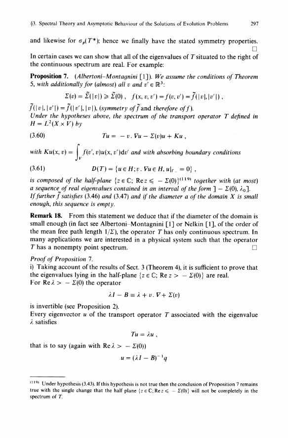
§3. Spectral Theory and Asymptotic Behaviour of the Solutions of Evolution Problems 297
and likewise for (J p( T*); hence we finally have the stated symmetry properties. o
In certain cases we can show that all of the eigenvalues of T situated to the right of the continuous spectrum are real. For example:
Proposition 7. (Albertoni-Montagnini [1]). We assume the conditions of Theorem 5, with additionally for (almost) all v and v' E ~3:
E(v) = £(Ivl);;:: £(0), f(x, v, v') =f(v, v') =j(lvl,lv'I),
j( 1 v I, 1 v' I) = j( 1 v'I, 1 vi), (symmetry of j and therefore off)· Under the hypotheses above, the spectrum of the transport operator T defined in H = L2(XX V) by
(3.60) Tu = - v. Vu - E(v)u + Ku,
with Ku(x, v) = Lf(V I, v)u(x, v')dv' and with absorbing boundary conditions
(3.61) D(T)= {uEH;v. VUEH,uir- =O},
is composed of the half-plane {z E C; Re z::;; - 1'(0) }(119) together with (at most) a sequence of real eigenvalues contained in an interval of the form] - 1'(0), ..10 ].
If further j satisfies (3.46) and (3.47) and if the diameter a of the domain X is small enough, this sequence is empty.
Remark 18. From this statement we deduce that if the diameter of the domain is small enough (in fact see Albertoni-Montagnini [1] or Nelkin [1], of the order of the mean free path length 1/1'), the operator T has only continuous spectrum. In many applications we are interested in a physical system such that the operator T has a nonempty point spectrum. 0
Proof of Proposition 7. i) Taking account of the results of Sect. 3 (Theorem 4), it is sufficient to prove that the eigenvalues lying in the half-plane {z E C; Re z > - E(O)} are real. For ReA. > - 1'(0) the operator
AI - B == A + v. V + E(v)
is invertible (see Proposition 2). Every eigenvector u of the transport operator T associated with the eigenvalue A satisfies
Tu = AU ,
that is to say (again with ReA. > - 1'(0))
u = (U - B)-lq
(119) Under hypothesis (3.43). If this hypothesis is not true then the conclusion of Proposition 7 remains true with the single change that the half plane {z E C; Re z:s:; - 1'(O)} will not be completely in the spectrum of T.
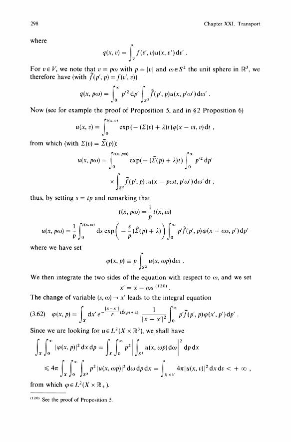
298 Chapter XXI. Transport
where
q(x, v) = Lf(V" v)u(x, u')dv' .
For VE V, we note that v = pw with p = Ivl and WES 2 the unit sphere in 1R 3, we therefore have (with j(p', p) = f(v', v))
q(x, pw) = foo p'2 dp' f j(p', p)u(x, p'w')dw' . o S2
Now (see for example the proof of Proposition 5, and in § 2 Proposition 6)
f'(X'V)
u(x, v) = 0 exp( - (E(u) + Ie)t)q(x - vt, v)dt ,
from which (with E(v) = £(p)):
u(x, pw) = f~(x,PW) exp( - (£(p) + ),)t) fooo p'2 dp'
x f j(p', p).u(x - pwt, p'w')dw'dt, S2
thus, by setting s = tp and remarking that 1
t(x, pw) = - t(x, w) p
1 f'(x,w) (s - ) foo -u(x, pw) = pods exp - p (E(p) + Ie) 0 p'f(p', p)qJ(x - ws, p')dp'
where we have set
qJ(x, p) == p f u(x, wp)dw . 52
We then integrate the two sides of the equation with respect to w, and we set
x' = x - WS (120) •
The change of variable (s, w) -+ x' leads to the integral equation
(3.62) qJ(x, p) = dx' e--p-(i(p)H). ,2 p'l(p', p)qJ(x', p')dp' . f Ix-x'i 1 fX x lx-xl 0
Since we are looking for uEL2(X x 1R3 ), we shall have
Ix La) I qJ(x, p)12 dx dp = Ix Loo p21 Is2 u(x, wp) dw 12 dp dx
~ 4n f foo f p21 u(x, wp)1 2 dw dp dx = f 4nl u(x, vW dx dv < + CfJ , x 0 52 X x V
from which qJ E U(X x IR+).
(120) See the proof of Proposition 5.
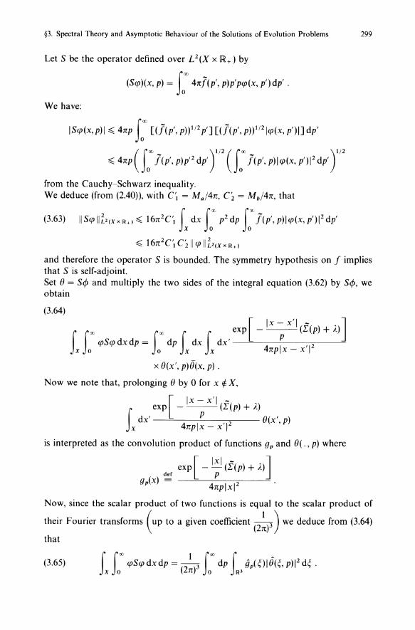
§3. Spectral Theory and Asymptotic Behaviour of the Solutions of Evolution Problems 299
Let S be the operator defined over e(X x IR+) by
(S<p)(x, p) = fooo 4nJ(p', p)p'p<p(x, p')dp' .
We have:
IS<p(x,p)l::S; 4np too [(J(p', p))1/2p'] [(](p', p))1/21<p(x, p')I] dp'
::s; 4np (too J(p', p)p'2 dP') 1/2 (fooo J(p', p)I<p(x, p'W dp' yl2
from the Cauchy-Schwarz inequality. We deduce (from (2.40)), with C'I = Ma/4n, C z = Mb/4n, that
(3.63) IIS<plli2(xxn;l+)::S; 16n2C'. L dx tx, p2dp t"'J(P',P)I<P(X,P') 12 dP'
::s; 16n2C'I Czll<plli2(xxn;l+)
and therefore the operator S is bounded. The symmetry hypothesis on f implies that S is self-adjoint. Set 0 = ScjJ and multiply the two sides of the integral equation (3.62) by ScjJ, we obtain
(3.64)
exp [ _lx-X'I(£(p)+.Ie)]
f f oo <pS<pdxdp = foo dp f dx f dx' 4 f _ '12 X 0 0 x x np x x
x O(x', p)O(x, p) .
Now we note that, prolonging (J by 0 for x ¢: X,
[ Ix - x'i -f exp - (l'(p) + .Ie)
dx' 4 IP '12 (J(x',p) x np x - x
is interpreted as the convolution product of functions gp and (J(., p) where
exp [ - ~ (£(p) + ),)] deC p
gp(X) = 4nplxl 2 •
Now, since the scalar product of two functions is equal to the scalar product of
their Fourier transforms (up to a given coefficient ~) we deduce from (3.64) (2n)
that
300 Chapter XXI. Transport
Calculate
by setting x = m with rE~+, UES2, and ~ = sw, we obtain:
gp(sw) = foo dr f -41 exp(- (£(p) + A)~ - irs(u .w))du o S2 np P
and by setting J1 = u . w,
gp(sw) = 21 foo dr f+ 1 exp( - (£(p) + A) ~ - irsJ1) dJ1 P 0 -1 P
1 f+ 1 dJ1
="2 - 1 (£(p) + A) + iSJ1p .
(since ReA. + £(p) > 0(121) this integral is convergent). Now if A is not real the imaginary part of gp(sw) will be of constant sign and never zero, which contradicts equation (3.65) whose left-hand side is always real. We therefore have proved that all of the eigenvalues lying in the half-plane {Re z > - £(O)} are real. ii) If J also satisfies (3.46) and (3.47), then by application of Proposition 5, we obtain that the sequence of eigenvalues A such that Re A > - £(0) is empty if the diameter of X is small enough. We shall verify this here - by using the hypothesis 17(v) ;;:: 17(0), which is stronger than (3.48), which allows us to simplify the proof of Proposition 5. Rewriting equation (3.62) in the form cp = K;.cp, we see that if A is an eigenvalue of the transport operator T, then 1 is an eigenvalue of the operator K;.. Now, we easily verify(l22) that the norm of the operator K;. in L 2 (X X ~ + ) satisfies
IIK;.1I 2 :::;sup (ff I _1 '12exp(-£(P)+AIX-X'I)P'l(P',P)dX'dP')' x.p Xx Hi+ X X P
s~~(ff I _1 '12exp(-£(P)+AIX-X'I)P'l(P',P)dXdP). X,p Xxlli+ x X P
Now £(p) + A > 0 and consequently
( 17(p) + A ) exp - P Ix - x'i :::; 1 .
Now we deduce (with (3.46), (3.47)) that
IIK;.112:::; sup(foo P'l(P',P)dP') sup (foo P'l(P',P)dP) p>O 0 p'>O 0
(121) As a consequence of the supplementary hypothesis made that 0 is a global minimum of 1:. (122) See the proof of inequality (3.63).
§3. Spectral Theory and Asymptotic Behaviour of the Solutions of Evolution Problems 301
Therefore, when
C l C2(4na)2 < 1
K). does not have an eigenvalue equal to 1 (V A such that £(p) + A > 0) and consequently the transport operator T does not have an eigenvalue greater than - £(0). 0
6. The Spectrum of the Transport Operator in a Band. The Lehner-Wing Theorem
We are interested in the following one-dimensional (x E IR) problem, with
Ko u(x, 11, t) = J: 11 u(x, 11', t) dl1', dJ1' being the Lebesgue measure over] -1, + 1 [:
{ ~~ + 11 au + u = :. Kou , (It ax 2
-a~x~a, -1~11~1, t~O, O<a<oo, (3.66)
where u = u(x, 11, t) is an unknown function satisfying the following boundary conditions:
(3.67)
(3.68)
u( - a, 11, t) = 0, 11 > 0, t ~ 0 ,
u(a, 11, t) = 0, 11 < 0, t ~ 0 ,
and also the initial condition
(3.69) u(x, 11, 0) = uo(x, 11), Ixl ~ a, 1111 ~ 1 .
We assume that c > O. This problem is a particular case of problem (2.1) with n = 1, X =] - a, a[, V = [- 1, 1], /-: playing the role of v. Equation (3.66) is obtained from the general transport equation (1.1) in the open subset of 1R3 (called a "band")
{(Xl,X2,X3)EIR3; IXll < a}
when the velocity space V is reduced to the sphere(l23) of radius unity (the unit being the modulus of the neutron velocity, which reduces to fixing the unit of velocity)(l24), when 17 is a positive constant which we take equal to 1 (which reduces to fixing the unit oflength equal to 1/17) and the collision nucleus equal to a positive constant c, (therefore the collision is independent of the modulus of velocity of the incident neutron, and of the outgoing neutron, of the incident angle of the neutron on the nucleus and the angle between the incident and exit velocities: the diffusion
(123) We then say that the transport equation is monokinetic. (124) We assume that V = S2 is equipped with the probability measure (equal to the surface measure divided by 4n).
302 Chapter XXI. Transport
is isotropic). We then easily show(\Z5) that the resolution of equation (1.1) in the band of 1R3 , with absorbing boundary conditions, with S = 0 and the initial condition Uo only depending on Xl (in variance under translations parallel to Oxz X3) is equivalent to the resolution of equations (3.66) to (3.69) in the interval ] - a, + a [ of IR, /1 being the projection of the neutron velocity (with I v I = 1) on to the axis Ox 1.
From Theorem 4, we already know that the operator T defined in H = LZ(] - a, a[ x [- 1, 1]) by
(3.70) {i) (Tu)(x, /1) = -/1 :: (x, /1) - u(x, /1) + ~ r: u(x, l1')dl1' ,
ii) D(T) = {UEH; /1 :: EH, u(w, /1) = 0 if £/1 < 0, £ = ± 1} has a continuous spectrum in the half-plane {Re z ~ - 1} and (possibly) a sequence of eigenvalues of finite multiplicity in the half-plane { - 1 ~ Re z}. On the other hand we can show, as in Proposition 7, that these eigenvalues (if they exist) are real. In fact, for the first time, we can confirm the existence of these eigenvalues:
Proposition 8. The transport operator T defined in (3.70) has a non empty sequence of real eigenvalues in the interval] - 1, c - 1 [ and a continuous spectrum in the half plane {Rez ~ - l}.
Remark 19. Problem (3.66) to (3.69) is very classical because of its simplicity for modelling certain physical applications. It is also here that the spectral theory has been completely made for the first time. A great many of the general proofs relative to the §3 may be inspired by those relative to this particular case. The only difference with the general case (and this is fundamental) concerns the real valuedness of the eigenvalues and their existence. D
Proof of Proposition 8. Firstly, we remark with the help of the Cauchy-Schwarz inequality that
(3.71) Re(Tu, u) ~ (c - 1)llu liZ
and consequently that the operator T + (l - c)J is dissipative. It follows that the type ofthe semigroup (G 1 (t)) generated by Tis less than or equal to (c - 1) and that the spectrum of T lies in the half-plane {Re z ~ c - l}. We then proceed in a manner analogous to the proof of Proposition 7. For A and u(x, /1) to be eigenvalue and eigenfunction of the operator T, that is,
(3.72)
i) -/1::(X'/1)-U(X'/1)+~f:ll u(x,/1')d/1' = AU(X,/1) , (uED(T)),
ii) u( - a, /1) = 0 if /1 > 0 ,
iii) u(a, /1) = 0 if /1 < 0 ,
(125) See Bussac-Reuss [1] or Weinberg-Wigner [I].
§3. Spectral Theory and Asymptotic Behaviour of the Solutions of Evolution Problems 303
it is necessary and sufficient that
der 1 f+ I q(x) = 2 -I u(x, /1)d/1
be the solution in L 2( - a, + a) of
(3.73) q(x) = 5:. f+a E((A + l)lx - sl)q(s)ds 2 -a
where E denotes the transcendental function
E(t) = e I' - = e 91 - • der II -~ d/1 foc - de
o /1 I e In effect (3.72) i) implies
au /1 ax + (A + l)u = cq ,
that is,
1 fX A+ I u(x, /1) = - e--I'-(X-S) cq(s) ds for /1 > 0
/1 -a
1 IX A+ I u(x, /1) = - e - -I'-(X - s) cq(s) ds /1 a
= ~ fa exp ( - A + llx - sl)cq(S)dS for /1 < 0 . 1/11 x 1/11
We then deduce
1 II d/1 fX (A + 1 ) q(x) = 2 - exp - ~- (x - s) cq(s)ds o /1 -a /1
+ - - exp - ~-Ix - sl cq(s)ds 1 fO d/1 fa ( A + 1 ) 2 -11/11 x 1/11
1 II d/1 f+a ( A + 1 ) = - - exp - ~-Ix - sl cq(s)ds 2 0 /1 -a /1
from which we have (3.73). By an argument similar to that in Proposition 7 (extending q by 0 outside] - a, a [) we show that A is necessarily real. Let KA be the selfadjoint operator defined in L 2( - a, + a) by
C f+a Kd(x) = 2 -a E((A + 1)lx - sl)f(s)ds .
The kernel of the operator KA is not a regular function (for A > - 1): in effect:
100 dr E((A + l)lx - sl) = e- r - -+ + 00
u+ 1)lx-sl r x -+ S ,
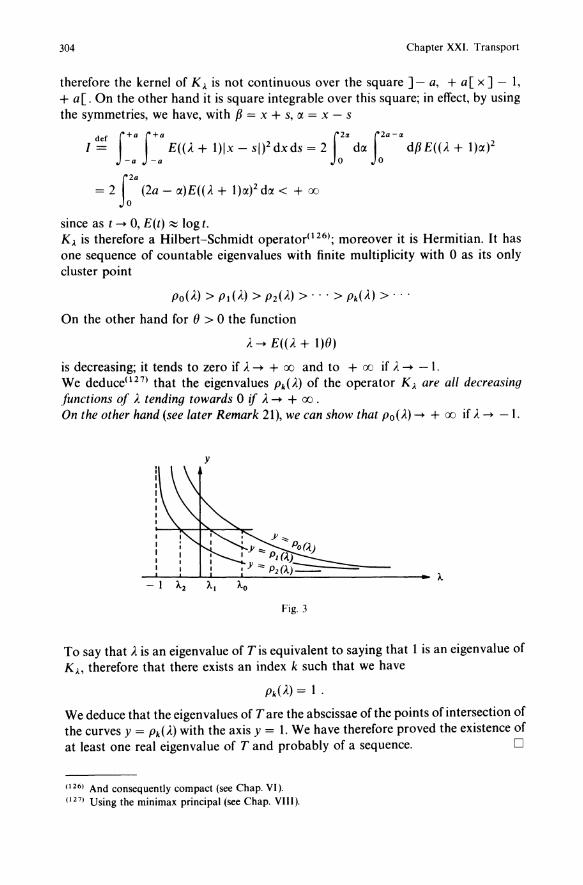
304 Chapter XXI. Transport
therefore the kernel of K .. is not continuous over the square] - a, + a[ x] - I, + a[. On the other hand it is square integrable over this square; in effect, by using the symmetries, we have, with f3 = x + s, a = x - s
d f f+a f+a f2a f2a-a I ~ -a -a E(o. + 1)lx - sl)2 dxds = 2 0 da 0 df3 E(o. + l)a)2
= 2 J:a (2a - a)E(o. + l)a)2 da < + 00
since as t -+ 0, E(t) ~ log t. K .. is therefore a Hilbert-Schmidt operator(126); moreover it is Hermitian. It has one sequence of countable eigenvalues with finite multiplicity with 0 as its only cluster point
Poo.) > pdA) > P2(A) > ... > Pko.) > ...
On the other hand for () > 0 the function
A -+ E(o. + 1)()
is decreasing; it tends to zero if A -+ + 00 and to + 00 if A -+ - I. We deduce(127) that the eigenvalues Pk(A) of the operator K .. are all decreasing functions of A tending towards 0 if A -+ + 00 .
On the other hand (see later Remark 21), we can show that Poo.) -+ + 00 if A -+ -1.
y
Fig. 3
To say that A is an eigenvalue of T is equivalent to saying that 1 is an eigenvalue of K .. , therefore that there exists an index k such that we have
Pko.) = 1 .
We deduce that the eigenvalues of Tare the abscissae of the points of intersection of the curves y = pdA) with the axis y = 1. We have therefore proved the existence of at least one real eigenvalue of T and probably of a sequence. 0
(126) And consequently compact (see Chap. VI). (127) Using the minimax principal (see Chap. VIII).
§3. Spectral Theory and Asymptotic Behaviour of the Solutions of Evolution Problems 305
Remark 20. The result of the nonexistence of eigenvalues (see Nelkin [1]) established in Proposition 7 concerns an open bounded set X of 1R3 of sufficiently small diameter and regular given data Land f In the present example «3.66) to (3.69» as in Proposition 7, the open set X is bounded (] - 1, + 1 [) and the data Land f are very regular (and even constant). On the other hand, it is an example in IR instead of 1R3; the proof is not transferable since 1/lxl is integrable in 1R3 but not in IR. Physically, this can be explained since the example considered here models a phenomenon in a band, therefore in an unbounded (in fact infinite) domain of 1R3. D
Remark 21. We define on operator K in H = L 2 (] - a, + a [) by
(Kw)(x) = f:: k(x, y)w(y)dy, VWEH,
where the kernel k is assumed symmetric and strictly positive:
k(x,y) = k(y,x) > 0, VX,yE] - a, + a[.
We know(128) that the operator K is bounded in L2(] - a, + a[) if
M = max f+a k(x, y)dy < + 00 . Ixl<:;a -a
We then have
IIKII:::;M.
If p denotes the spectral radius of K, we have
(Id p:::; IIKII:::; M.
On the other hand if K is compact, p is the largest eigenvalue of the operator K. From the minimax principal(129), we have
p = max (Kw, w) . Ilwll= 1
By choosing w = ~, we deduce v' 2a
1 f+a f+a P~2a -a -a k(x,y)dxdy,
from which
1 f+a f+a f+a -2 k(x, y) dx dy :::; p :::; max k(x, y) dy .
a -a -a Ixl<:;a -a
By applying inequalities (I tl and (I2) to the operator K A. defined in the proof of
(128) See Chap. VI. (129) See Chap. VIII.
306 Chapter XXI. Transport
Proposition 7 (with A = 0), we see that if
(3.74) max - E(lx - sl)ds < 1 , f +a C
Ixl';;a -a 2
then the largest eigenvalue AO of the operator T defined in (3.70) is negative and problem (3.66) to (3.69) is subcritical. If on the other hand
(3.74)' - - E(lx - sl)dsdx > 1 1 f+a f+a C
2a -a -a 2
then AO > 0 and problem (3.66) to (3.69) is supercritical. We can therefore, in this particular case, make explicit the relation between c and a leading to criticality. Finally, we verify with (1 2 ) the property stated for Proposition 8:
Po(A) ~ ~ f2a (2a - IX)E«(A + l)lX)dlX--+ + 00 for A--+ - 1 . 0 2a 0
7. Study of the Spectrum of the Transport Operator in the Whole Space: X = IRn
We consider the transport operator T defined in H = L 2([R" X V) by
{
i) Tu(x, v) = - v. Vu(x, v) - E(v)u(x, v) + Lf(V" v)u(x, v')dv' ,
(3.75) XE [R", VE V, uED(T),
ii) D(T) = {uEH; v. VUEH}
Since we are taking the case of the whole space, that is, X = [R", we see that we can use the Fourier transform to characterise the spectrum of T. Let B be the operator defined by
{ BU= -v.Vu-E(v)u, D(B) = {uEH; v. VUEH} ,
and K the integral operator
(3.76) (Ku)(x, v) = Lf(V" v)u(x, v')dv' ;
occurring in (3.75) and therefore
T= B + K.
We assume that E(v) and the collision nucleus f(v', v) are independent of X(l30) and that the operator K defined in (3.76) is compact(131) from L2(V) into itself (132).
(130) This is indispensable for the method used here. (131) This operator is compact in L2(V) when V is bounded and f regular (fe~O(Vx V)), or also, for V bounded or not, when fe e(V x V) (then K is a Hilbert-Schmidt operator). (132) It cannot be, in return, compact from L2(X x V) into itself.
§3. Spectral Theory and Asymptotic Behaviour of the Solutions of Evolution Problems 307
Contrary to the case where the open set X is bounded (see §3.3) the operator
R(t) = r ds t Gdr)KG(s - r)KG(t - s)dr ,
where G and G1 denote the semigroups generated by the operators Band B + K, is not compact in H = L2([Rn X V)(133).
Therefore the difference between the spectra of Band (B + K) does not necessarily reduce to eigenvalues of finite multiplicity. We have seen (§3.2.1) that the spectrum of the operator B = - V' V - 1: is given by
a(B) = PEC, ReAE - Im1:}
and that, if G(t), t > 0, denotes the semigroup generated by B, we have
a(G(t» = et(J(B) = {eo., AEa(B)} .
Theorem 8. Let X = [Rn, V = V with 0 E V with the Lebesgue measure dJl = dv. We assume that 1: satisfies (3.18) and 0 ~ 1:(0) ~ 1:(v), V v E V, that the positive function f = f(v', v) is independent of x, symmetric in v and v', and satisfies the bound (2.40):
(3.77) tf(V', v)dv' ~ M (134), VVE V,
and such that the operator K defined by (3.76) is compact in U(V)(135). Then there exist constants a ;:::, 0 and b ~ 0 such that the spectrum of the operator T = B + K defined by (3.75) and (3.76) in L2([Rn X V) is contained in the following set A:
A = {ZEC, b ~ Rez ~ -1:(0)} u {ZEC, -1:(0) < Rez ~ -1:(0)
+ M, Ilmzl ~ a} .
Proof Since the operator T is the infinitesimal generator of a group and since we have the inequality
Re(Bu, u) ~ - 1:(0) II U 112 ,
it is immediate(136) that the spectrum of (B + K) is contained in the band {b ~ Re Z ~ - 1:(0) + II K II}, and in particular in the band {b ~ Re Z ~ - 1:(0) + M} since II K II ~ M from (3.77). It remains to show that in the band
{ - 1:(0) < Re Z ~ - 1:(0) + M} ,
the points A of the spectrum of B + K satisfy the uniform bound
IlmAI ~ a.
(133) It is the same in the case (studied in the following section) where X is the complement of an open set. (134) Note that this condition is insufficient for the operator K to be compact; it is sufficient to take f(v', v) of the form f(v', v) = l(v - v') for V = [R3JEL 1([R3) to see it.
(135) Which is true in particular if r (f(v', V))2 dvdv' < + 00.
Jvxv (136) In effect, the operator B + K + 1"(0) - II K II is dissipative and the infinitesimal generator of a (contraction) semigroup.
308 Chapter XXI. Transport
We know that for Re Je > - ,[(0), the operator AI - B is invertible. It is sufficient therefore to prove that for 11m Je I > a, the operator (Je I - B) - 1 K has norm strictly less than 1. This proves that the operator I - (A - B)-I K (and consequently the operator AI - B - K) is invertible and therefore that A ¢: a(B + K). F or this, we use the Fourier transformation. Let WE H be given and u = (Je - B)-I W, we have
A w«(, v) u( J: v) - .
1." - Je + iv. ( + .[(v) ,
now, if w = Kg, where g E H is given, we have
( 1 B)-I K d A(J: ) f f(v', v)g«(, v') d' u = A - g an u 1." v = V • v Je + .[(v) + iv. (
It is sufficient, from the Plancherel theorem, to show that there exists a constant e < 1 such that
IluIIL2(~nxv) ~ OllgIIL2(~nxv), VgEL2(~n X V).
For (E ~n given, we introduce the operator K ~ defined by
(K),g)(v) == r f(v', v)g(v') dv' ~ J v Je + .[(v) + iv. (
and it is sufficient for this to show that K ~ is a bounded operator in L 2( V) with
(3.78)
Now
sup II K ~ II ~ 0 < 1 . ~
II K),II ~ ( r f(v', v) d ,)112 ( f f(v', v) d )112 ~ '" m~x JvIJe+.[(v)+i(.vl v m,~x vIJe+.[(v)+i(.vl v
We deduce, by continuing as in Nishida-Imau [1], that when I A.I + I (1-> + 00,
II K ~ II -> 0 from which we have (3.78). We therefore have shown that there exists a constant a > 0 such that if Je E a(B + K) with ReA > - ,[(0), then 11m Je I ~ a. We now give another case, which is particularly interesting for applications, of the spectrum of the transport operator presented here in the Banach space L 1 (~n X V).
Theorem 8'. Let X = ~n, V be a shell: V = {VE ~n, 0 < Vrn ~ Ivl ~ l} with the Lebesgue measure; we assume that .[ and f satisfy (3.18) and (2.40) respectively and that .[(x, v) and f(x, v, v') are zero for all x outside of a compact set K(137). With
M('[) ~ esssup _1_ .[(x, v), M(f) ~ esssup _11 I r f(x, v, v')dv' , (X.V)E~nXV IVrnl (X.t')E~nxv Vrn Jv
(137) Therefore we have modelled a situation where K is occupied by a medium (characterised by Land fl. surrounded by a vacuum.
§3. Spectral Theory and Asymptotic Behaviour of the Solutions of Evolution Problems 309
we further assume that
(H) (diam K)M(I) < 1 and (diam K)M(f) < 1 .
Then the transport operator Tin L 1 (/R" x V) is the infinitesimal generator of a group (C1 (tn EG;! such that II Cdt) II :;:; M, 'it ? 0(138); the spectrum (J(T) of T is composed of:
where:
(Jr(T) = i/R is the residual spectrum of T, (J P(T) (the point spectrum) is a finite set(139) of isolated points in a band:
{z E IC, - C :;:; Re Z < O}, c positive constant .
We refer to Emamirad [1] for the proof of this Theorem. Note that here the residual spectrum "replaces" the continuous spectrum; this is due to the passage from the space L2(X x V) to U(X x V). This theorem is to be compared with Theorem 3 (largen's Theorem) and also with Proposition 5 (hypothesis (H) is true when the compact set K is sufficiently small). We can generalise Theorem 8' by:
Theorem 8/1. We assume that in /R" x V(140), the given data f and I satisfy (2.40) and IE L 00 (/R" x V), further with f and I with bounded support in x; let X be an open bounded convex set in /R" containing these supports. We denote respectively by T = TG;!n, Tx and Tx the transport operators in U(/R" x V), in U(X x V) with "absorbing conditions": D(Tx) = rUE WP(X x V), ulr _ = O}, in U(X x V), with the condition
D(Tx) = rUE WP(X x V), ulr+ = O}, for pE[l, + 00 [. Then
i) (J( T) = ((J( Tx) n {z E C, Re z < O} ) U i/R U ((J( Tx ) n {z E C, Re z > O} )
ii) (J p(T) n {z E IC, Re z =f. O} = ((J p(Tx) n {z E C, Re z < O} )
u((Jp(Tx)n{zEC,Rez >O})
where (J p(T) denotes the point spectrum (the set of eigenvalues) of the considered operator.
Proof The proof is based on the following remark: the equation - I v I :~ - AU
= q (with q given in U) on a half-line (/R + or /R - ) is resolved in U:
1) without a condition at x = 0, if Re A> 0 in /R- and if Re A < 0 in /R+; 2) with a condition at x = 0, if ReA > 0 in /R + and if ReA < 0 in /R - .
(138) The corresponding system is therefore "subcritical" (or "critical"). (139) Possibly empty. (140) With a positive Radon measure Jl over ~n such that V = supp Jl and Jl( {O}) = 0 (see §2). We emphasise that V is here an arbitrary closed set of ~n (not necessarily a shell in the unit ball of ~n).
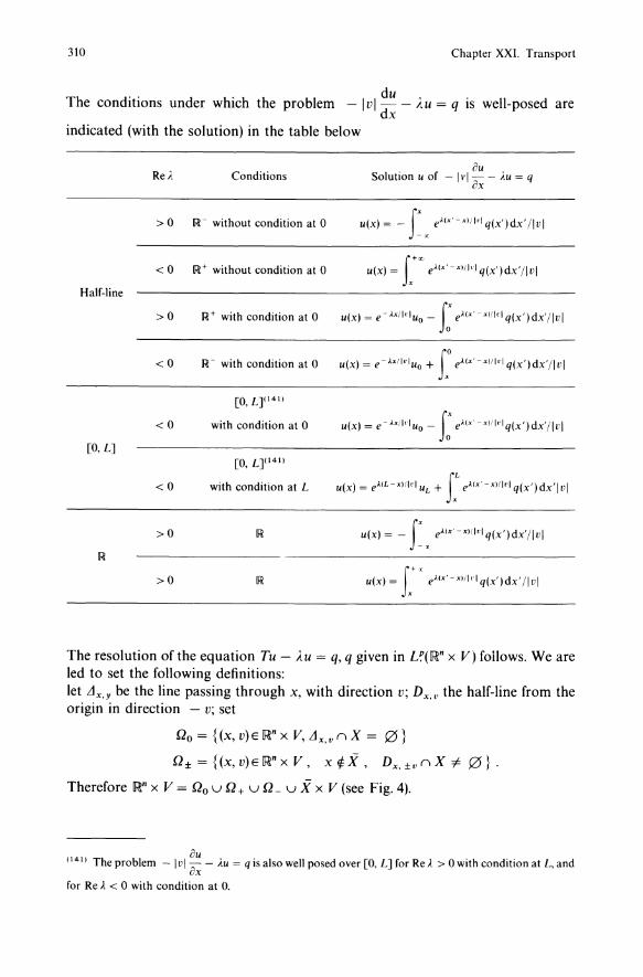
310 Chapter XXI. Transport
The conditions under which the problem - Ivl du - AU = q IS well-posed are dx
indicated (with the solution) in the table below
Half-line
[0, L]
Re;' Conditions
> 0 IR - without condition at 0
< 0 IR+ without condition at 0
au Solution u of - I v I -:;- - i.u = q
ex
f+X
u(x) = x e'(x'-x)iI.1 q(x')dx'/lvl
> 0 IR+ with condition at 0 u(x) = e-hil.'l uo - f: e'(X'-X)/I"lq(x')dx'/lvl
< 0 IR- with condition at 0 u(x) = e-h!I'l uo + f: e>\x'-X)/I'lq(x')dx'/lvl
[0, L](l41)
<0 with condition at 0
[0, L](141)
<0 with condition at L
>0 u(x) = - 1:x e>\x'-x)!I'lq(x')dx'/lvl
>0 f+x
u(x) = x e'(X' -x)/I"1 q(x')dx' Ilul
The resolution of the equation Tu - AU = q, q given in U(IR" x V) follows. We are led to set the following definitions: let L1 x,y be the line passing through x, with direction v; Dx,L' the half-line from the origin in direction - v; set
Qo = {(x, V)E IR" x V, L1x.v n X = 0}
Q±={(X,V)EIR"XV, x¢X, Dx.±vnX#0}.
Therefore IR" x V = Qo u Q+ u Q_ u X x V (see Fig. 4).
au (141) The problem - I v I - - i.u = q is also well posed over [0, L] for Re A > 0 with condition at L, and
ax for Re A < 0 with condition at O.
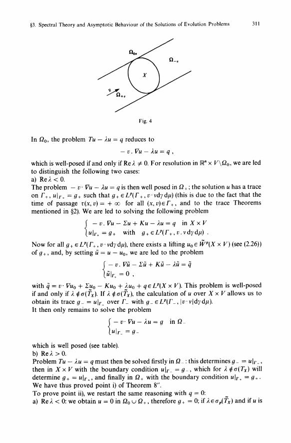
§3. Spectral Theory and Asymptotic Behaviour of the Solutions of Evolution Problems 311
Fig. 4
In Qo, the problem Tu - AU = q reduces to
- v. Vu - AU = q ,
which is well-posed if and only if Re A i= O. For resolution in [Rn x V\Qo, we are led to distinguish the following two cases: a) ReA. < O. The problem - V' Vu - AU = q is then well posed in Q + ; the solution u has a trace on r+, ulr+ = g+ such that g+ EU(r h v'vdyd)1) (this is due to the fact that the time of passage !(x, v) = + 00 for all (x, v) E r +, and to the trace Theorems mentioned in §2). We are led to solving the following problem
{ -v. Vu - 1:u + Ku - A.U = q in X x V
ulr+ =g+ with g+EU(r+,v.vdyd)1).
Now for all g + E U( r+, V· vdy d)1), there exists a lifting Uo E WP(X x V) (see (2.26» of g +, and, by setting u = u - uo, we are led to the problem
{:- v. Vu - 1:14 + Ku - AU = q ulr+ = 0 ,
with q = V· VUo + 1:uo - Kuo + AUo + q E U(X x V). This problem is well-posed if and only if A ¢ a(Tx). If A ¢ a(Tx), the calculation of u over X x V allows us to obtain its trace g _ = UIL over L with g _ E U(L, I V· vldy d)1). It then only remains to solve the problem
{ -v' Vu - A.U = g in!L
UIL = g-
which is well posed (see table). b) ReA. > O. Problem Tu - AU = q must then be solved firstly in Q - : this determines g - = u Ir _ , then in X x V with the boundary condition u Ir _ = g _, which for A ¢ a(Tx) will determine g + = u Ir +' and finally in Q + with the boundary condition u Ir + = g + .
We have thus proved point i) of Theorem 8". To prove point ii), we restart the same reasoning with q = 0: a) ReA < 0: we obtain u = 0 in Qo u Q+, therefore g+ = 0; if AEap(Tx ) and if u is
312 Chapter XXI. Transport
the eigenvector of Tx for A, the trace g _ = U Ir _ of u over r _ (with g _ E U( r - , d[~ : see Appendix §2) allows us to obtain u on Q _, with finally u E WP(X X V). b) ReA> 0: we obtain u = 0 in Q o u Q_ therefore g_ = 0 and we continue in a way analogous to the preceding case. 0 We easily verify that A with Re ..1.= 0 can be an eigenvalue of the operator Tin IRn x V if and only if there exist u E WP(lRn x V), u ¢ 0, with u = 0 in Q o u Q + u Q_
and satisfying:
{-v.vu-rU+KU-AU=O, UEWP(XXV) ,
ulr + = ulr _ = 0 .
We see in particular that the criticality problem for TR", i.e. that of determining if there exists an eigenvalue A > 0 (or A with largest real part positive, associated with a positive eigenvector) is reduced to the problem of criticality of the operator Tx , which emphasises the importance of spectral study of the transport operator Tx with absorbing boundary conditions. We also note that the inhomogeneous boundary conditions with U Ir ± E LP (r ±, I v . v I dy dJ.L) occur naturally in these types of problem. We finally note that in the case of Theorem 8' (and also in all of the cases called "subcritical") the point spectrum of the operator TR" is that of the operator Tx .
o We now take the one-dimensional case (n = 1) and for V = [ -1, + 1] where we shall make explicit the results of Theorem 8. We look for the spectrum of the operator T defined in H = L 2(1R x [ -1, 1]) by
{i) (Tu)(x, J.L) = - J.L :: (x, J.L) - u(x, J.L) + ~ f:: u(x, J.L')dJ.L', c > 0 ,
(3.79) {au } (142)
ii) D(T) = UEH; J.L ax EH .
Proposition 9. The spectrum of the operator T defined in (3.79) in H is composed of the axis {ZEC; Rez = -l} and the real interval [-1, c - 1] (see Fig. 5). All of the points of this set are elements of the continuous spectrum of T.
Proof We start by proving that a(T) is contained by
S = {z E C; Re Z = - I} u {z E IR; - 1 :::;; Z :::;; C - I} ;
for given gEL 2(1R x] -1, 1 [), we consider the resolvent equation:
au c f+1 AU(X, J.L) + J.L ax (x, J.L) + u(x, J.L) -"2 -I u(x, J.L')dJ.L' = g(x, J.L) •
By Fourier transformation, we obtain
(3.80)
(142) We therefore use the hypotheses on V, E, K and f and the notation of the example of the band studied in §3.6, with the exception that here we take a infinite.
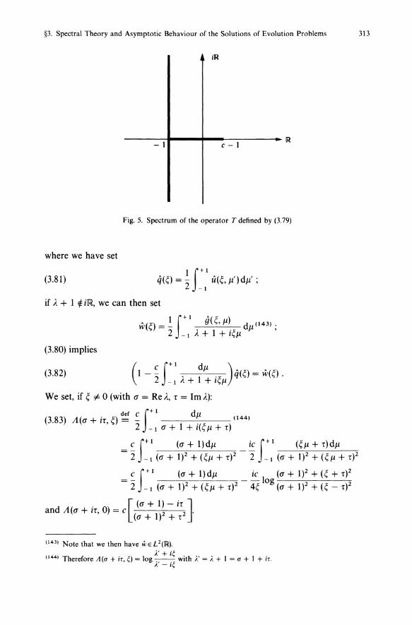
§3. Spectral Theory and Asymptotic Behaviour of the Solutions of Evolution Problems 313
ilR
- 1 c - I
Fig. 5. Spectrum of the operator T defined by (3.79)
where we have set
(3.81)
if A + 1 ¢ ilR, we can then set
W(~)=~f+1 g(~,J.l). dJ.l(143);
2 - 1 A + 1 + 1~J.l (3.80) implies
(3.82) ( C f+ 1 dJ.l ) • •
1 - 2: -I A + 1 + i~J.l q(~) = w(~) .
We set, if ~ #- 0 (with a = Re A, T = 1m A):
(3.83)
. [ (a + 1) - iT J and A(a + IT, 0) = c 2 2. (a + 1) + T
(143) Note that we then have WE L 2 (IR).
(144) Therefore A(u + ir, () = 10g~: ~ :~ with;: = A + 1 = u + I + ir.
314 Chapter XXI. Transport
We see that if T "# 0, the imaginary part of A(a + it, ~) is never zero, and consequently A(a + it) is never equal to 1; further lim A(a + iT, ~) = 0, therefore
~~ ± 00
1/(1 - A(a + it, mEL 00 (IR~), and
q(~)= W(~). EL2(1R). 1 - A(a + IT, ~)
Besides, we verify that for T = 0 c ~
(3.84) A(a, ~) = ~ arctan a + 1 '
therefore if a + 1 < 0, A(a, ~) < 0 and 1 - A(a, ~) is never zero. On the other hand, if a + 1 > C, we verify that
A(a, ~) :::; 0 < 1, 'v'~ E IR ,
and consequently we have shown that the intervals] - 00, - 1 [ and] C - 1, + 00 [
are part of the resolvent set of T. Finally, we have shown that the spectrum of T is included in the set S. We show that all of the points of S are, in fact, elements of the continuous spectrum, that is to say if A. E S, then
Ker(U - T) = Ker(iI - T*) = {O}
and on the other hand that the subspaces
Im(U - T) and Im(iI - T*)
are dense, but strictly included, in H = L 2 (IR x [ - 1, 1]). We remark that the set S is stable by conjugation:
and that the operator T* has the same structure as T since it is obtained by
I · 0 b 0 rep acmg J1 ox y - J1 ox· To show that Im(U - T) does not coincide with H, note that if the equation (U - T)u = f has a solution for all fE 9'(1R x [ -1, + 1]), then we have
u=(U- T)- l fE9'(lRx[-I, +1]).
It is therefore sufficient to show that for XES, there exists a tempered distribution u* which is non-zero and such that
Xu* - T*u* = 0 .
(Indeed, in this case if fE 9'(1R x [ -1, + 1]) (\ Im(U - T)
(f, u*) = (A.U - Tu, u*) = (u, Xu* - T*u*) = 0;
if Im(U - T) = H, we deduce that u* = 0 which is a contradiction: consequently Im(U - T) "# H). The construction of the distribution u* is inspired by the methods of Case-Zweifel [1], Chap. IV.
§3. Spectral Theory and Asymptotic Behaviour of the Solutions of Evolution Problems 315
i) Assume first of all that A = - 1 + ir. We verify that the kernel of AI - T is reduced to zero. Let u E H satisfy
au C f+ 1 (3.85) iru(x, 11) + 11 ax (x, 11) - 2 _ 1 u(x, J1') dil' = 0 .
Taking the scalar product of the two sides with u and taking the real part we
deduce (bY remarking that Re(1l ::' u) = 0 ):
~ L I f:l1 u(x, Il ' )dllf dx = 0 .
By returning to equation (3.85) we deduce
au f . 0 iru + 11 ax = 0 rom whIch u = .
We then look for the distribution u* in the form
ut.t(x, 11) = <P~(Il)eix~ with I~I > r (145)
with
(3.86) f+ 1
_ 1 <P~(Il) dll = 1 (146)
The relation
(( -1 + ir) _. T*)u* = 0
is written
(-1 - ir)u*(x, 11) - (11 :x u*(x, 11) - u*(x, 11) + ~ f:l1 u*(x, 11') dil' ) = 0 ,
that is to say
a C f+ 1 iru*(x, 11) + 11-;- u*(x, 11) + - u*(x, 11') dil' = 0
uX 2 -1
C f+ 1 i(r + 1l~)<P~(Il) + - <P~(Il')dJ1' = 0;
2 -1
(145) This condition is explained later. (146) <P; being a distribution over [I, + I] identified with a distribution over 1I\l" with support [- I, + I] (see Introduction of §2), the sense of (3.86) is given by
f+1
-I <P;(/l)d/l = (<P;(/l), I> = I
(where <, > denotes the duality C(II\l), C(II\l)). Note that this "normalisation" of the distribution u* is purely arbitrary.
316 Chapter XXI. Transport
from which, taking account of (3.86)
(r) c i ~+/1 cP~(/1)= -2~'
With the hypothesis Ir/~1 < I, we have (1X<5(Z + /1) )(Z + /1 ) = 0, and conse
quently, we obtain (for I ~ I > r)
ic I cP~(/1) = 2~ pv (r/~) + /1 + 1X<5«r/O + /1)
by determining IX so that the initial condition (3.86) is satisfied. This finally gives
. [iC I (iC ~ + r) . ] u~.t(x, /1) = Y(I~I - Irl)eIX~ 2~ pv /1 + (r/~) + I - 2~ log ~ _ r (j(/1 + (rim .
ii) We now consider the case A = a E] - I, C - I [ . We then look for the distribution u* (the solution of (a - T* )u* = 0) in the form
u*(x, /1) = cP~(/1)eix~ .
By putting this expression in the equation (a - T*)u* = 0, we find by setting
1 f+1 q(~) = - cP~(/1 )d/1 (see (3.81)) that we must have as in (3.82) and (3.84) 2 -I
( C ~ ) I - ~ arctan a + I q(~) = 0 .
For 0 < a + 1 ~ c, the function ~ ---+ I - Z arctan(~/(a + I)) is zero at two symme
tric points ~ + (a) and ~ _ (a) = - ~ _ (a); ~ + (a) is a decreasing function of a. On the other hand, we verify that
Finally we therefore obtain for every a E] - I, c - I] two independent distributions denoted ut+(U) and ut-(U) defined by:
o
Remark 22. Taking account of Theorem 8 and of Proposition 9, we cannot apply the criticality results here which were shown in §3.4 in the case of the discrete spectrum. We shall therefore make a direct study here to look at this idea. We shall first of all verify that if c ~ 1, then the operator T is dissipative in the spaces L2(lRx(-I, +1)) and U(lRx(-I, +1)). i) The space L2(1R x (-1, + I)).
§3. Spectral Theory and Asymptotic Behaviour of the Solutions of Evolution Problems 317
For every u E D(T), we have:
(Tu, u) = - (Ii ~~, u) - (u, u) + ~ t [If:11
u(x, li)dIi12JdX.
Now - (Ii ~~, u ) = 0, and by the Cauchy-Schwarz inequality,
~ t I f:11
u(x, li) d1i 1
2 dx~ t f:11
lu(x, IiWdli dx .
Hence we have: (Tu, u) ~ (c - l)(u, u) ,,-;; 0. ii) ThespaceLI(lRx(-I, +1)). The proof is analogous to that of the proof of Proposition 5, §2; see also Chap. XVII A, §3, Proposition 4. With the notation of these Propositions, we have for all uED(T):
+~ r dxf+1 dli'U(X,Ii')f+ 1 signoudli. 2JR -I -I
Now \ - Ii :~ , signo u ) = ° and since
<Tu,signou)"-;;(c-I) r IU(X,Ii)ldxdli' JGIX(-I. + I)
Hence follows the stated result. Since T is the infinitesimal generator of a group (G 1 (t)), t E IR, of class <'6'0, then for c"-;; 1, and t > 0, the semigroup (Gdt)Lo is a contraction semigroup. For c < 1, T + (I - c)J is also a dissipative operator, and we therefore have
II e(l-C)tG l (t) II ,,-;; 1, II Gdt) II ,,-;; e(c-l)t ,
in the spaces Z = Ll(1R x (-1, + 1)) and Z = L2(1R x (-1, + 1)). Therefore for all Uo E Z, the solution to the Cauchy problem in Z
{ du = Tu dt
u(o) = Uo
given by u(t) = G1 (t)uo is exponentially decreasing for t -+ + 00. The evolution problem is called subcritical. For c > 1 the study made above shows that the point (c - 1,0) E <C is the rightmost point of the spectrum of the operator Tin Z = L2(1R x (-1, + 1)) and also in Z = U(IR x (-1, + 1)). This implies that there exists a UoEZ such that II G1(t)uo liz is unbounded (as t -+ + 00). In effect if for every Uo E z, II G1 (t)uo II ,,-;; M"O for all t ~ ° (or t -+ + 00), then by the Banach-Steinhaus Theorem (see Chap. VI) there
318 Chapter XXI. Transport
will exist a positive constant M such that II G1 (t) II ~ M (for t ~ 0 or t -+ + 00),
which implies by the Hille-Y osida Theorem that spectrum of the operator T will be contained in the half-plane {z E 1[, Re z ~ O}. Therefore there exist initial conditions UoEZ for which the solution of the Cauchy problem in Z, u(t) = G1(t)uo has a norm (in Z) which tends to infinity as t -+ + 00 (147}. The evolution problem is called supercritical. The value c = 1 plays (as in §3.4) the role of a limit value. The problem is then called critical. D
Remark 23. The results generalise to the case of the monokinetic problem (V = sphere of ~n) in the whole space, that is to say the case where H = L 2 (~3 X S2) and:
Tu(x, w) = - w. Vu(x, w) - u(x, w) + 4c r u(x, w')dw' 1t JS2
(see Bardos-Cessenat [1], Ukai-Point-Ghidouche [1]). D
Remark 24. With the notation ofthe proof of Proposition 9, we can show that the distributions:
e±i~±(a}. x
u~±(a} (x, J.l) = U + 1 + iJ.l~±(u) for UE[ -1, c - 1] ,
and
u~.t(x, J.l) = Y(I~I_lrl)eiX~[ - ~~ vp J.l +\r/E) + (1 - ~~ log ~ ~: <>(J.l +~) ] for A. = - 1 + it, r E ~ ,
are generalised eigenfunctions of the operator T defined by (3.79) (see BardosCessenat [1]). Further we can show that this family of generalised eigenfunctions is total, that is to say that we have, for every regular function 4J E D(T):
qJ(x, J.l) = I~ I [( qJ, ut+ (a} > u~+ (a}(x, J.l) + (qJ, ut (a} > u~ _ (a} (x, J.l)] du
+ r dr r (qJ, ut,t>u~,t(x, /l)d~ (148} ,
JR JI~I>ltl (for a suitable normalisation of the generalised eigenfunctions u~," u~da} of T and
(147) By using the same reasoning as above with e-·"Gdt) replacing Gdt), for WE [0, C - I [. we can show that there exists a Uo E Z such that
II G1 (t)uo II ;" M.oe"" for t -+ + 00 .
(148) The notation (, > corresponds to the antiduality Y'(IR x [-1, + I]), Y"(IR x [-I, + I]); note that we wi\l also have a relation "similar" to Parseval's relation. Naturally the sense in which this formula is convergent would be made precise.
§3. Spectral Theory and Asymptotic Behaviour of the Solutions of Evolution Problems 319
ut,,, ut±(<r) of T*), and this decomposition diagonalises the operator T(this generalises the procedure of diagonalisation in the presence of a continuous spectrum, see Chap. VIII, §1):
(3.88)
{ (T<p) (x, J.1) = r~ 1 0"[ <<p, ut+(<r)U~.+(<r)(X' J.1) + <<p, ut-(<r)u~~(<r)(x, J.1)] dO"
+ r (-1 + ir)dr r <<p,ut,t)u~.t(x,J.1)d~ . D J~ JI~I>ltl
We shall now give, again in the monodimensional case studied in Proposition 9, some precise details on the asymptotic behaviour in the critical case (c = 1) already mentioned in Remark 22. We have:
Proposition 10. Let T be the transport operator in H = L2(1R x [ -1, + 1]) defined by (3.79) with c = 1 and (G 1 (t)) the semigroup generated by Tin H. Then for every gEH, we have
(3.89) lim II G1 (t)g IIH = 0 . ,~x
Proof Since (G1(t)ho is a contraction semigroup, it is sufficient to verify (3.89) over a dense subspace: for example the subspace of regular functions g of D(T) whose Fourier transform g is zero in a neighbourhood of zero. From Butzer-Berens [1], p. 79, we have for all gED(T), t > 0 and s > 0:
(3.90) G1 (t)g = -.- e'A(A - T)-I g)d), (149) . 1 f,+iX,
2m ,-ix
Let u = (A - T) - 1 g, then 11 satisfies (3.80) with c = 1. We deduce, by again setting
{
def 1 f + 1 dJ.1 A der 1 f + 1 A , ,
A(A.'~)=2 -1),+I+i~J.1' q(~)=2 _lu(~,J.1)dJ.1 (3.91) A 1 1 f+1 g(~, J.1)dJ.1
q(O= l-Ao.,~)2 -I A+ 1 +i~J.1' that is, using (3.80) again,
(380)' A(!, 1 (A 1 1 f+1 g(~,J.1) d) . u '" J.1) = A + 1 + i~J.1 g(~, J.1) + 1 - AU, 02 -I A + 1 + i~J.1 J.1 .
As we have seen, the function 1 - A (),' 0 is only zero for A E [ - 1, OJ. The solution A(~) of the equation
Ao., ~) = 1
(149) In the sense of Gdt)g = lim ---: e'A ((;' ~- T)~lg)d;'. 1 J.di' y-oo 21t'1 [~iy
320
is therefore real. From (3.84), we have (if I ~ I ~ nj2)
A(O=-~--1 . tan ~
Chapter XXI. Transport
Since the function g(~, /l) is by hypothesis identically zero in a neighbourhood of the origin there exists a constant b > 0 such that
- 1 ~ A( 0 ~ - b < 0
for all ~ outside of this neighbourhood; we deduce that the function
A-> 1 ~f+l g(~,/l)d/l 1 - A (A, ~) 2 _ 1 A + 1 + i ~ /l
is holomorphic in the half-plane {Rd ~ - b}. From (3.80)', u is therefore a holomorphic function in the same domain; it is therefore the same for u = (A - T) - 1 g. Consequently, in (3.91), we can replace the integral over the line {Re A = f.} by an integral over the line {Rd = - bj2}. We therefore deduce that for such a g,
Gdt) -> 0 for t -> + CXJ ,
and from this we have, by density, (3.89). 0
Remark 25. The result of Proposition 10 establishes that the solution u of the problem (critical case)
{au au 1 f+ 1 -;- + /l -;- + u = - u d/l', X E IR, /l E [ - 1, + 1] , ut uX 2-1 u(O) = 9
(3.92)
for gEL 2(1R x (-1, + 1)) (\ L 1 (IR x (-1, + 1)), satisfies II u(t) IIL2 -> 0 as t -> + CXJ
and also:
(3.93) f u(t)dxd/l = f gdxd/l, "It> 0 ,
the absorptions by the term u in (3.92) exactly compensate the creations by the
. . 1 f collIsIOn term"2 u d/l'.
The decrease of the L 2 norm therefore indicates that the solution u, while satisfying (3.93), spreads out in the whole space. This situation is fairly different from that of a bounded domain and of the band and this is the subject of the following remark. 0
Remark 26. In the case of the band (§3.6), the critical case corresponds to A(T) = 0; then the principal eigenfunction, relative to A(T), UA(T), is invariant under etT:
etT UA(T) = UA(T) •
In the case of the whole space IR, there is only a continuous spectrum and therefore
§3. Spectral Theory and Asymptotic Behaviour of the Solutions of Evolution Problems 321
no function u E L 2(/R x [ - I, + I]) which is an eigenfunction of T(150). Besides, and for example in the critical case, the function
u(x, 11) = 1
satisfies
au 1 f+ 1 11 - + u - - u dJ1' = 0 . ax 2-1
It is invariant under efT, but it is not in L2(/R x [ - I, + I]); this is a generalised eigenfunction. D
Remark 27. The generalisation of the result of Proposition JO in the case L 2(/Rn X sn -1) is established in Ukai-Piont-Ghidouche [I]. D
8. The Spectrum of the Transport Operator on the Exterior of an "Obstacle"
The essential result of this section is that if the spectrum of the operator T in the whole space conforms to the result established in Theorem 8, then the spectrum of the transport operator in the exterior of an "obstacle" is composed of the same set, plus possibly eigenvalues of finite multiplicity. Let F be a bounded closed set of /Rn (the obstacle) that we assume to be convex with regular boundary, and X the complement of F in /R n. We assume, as in the beginning of §3.7, the transport operator Tin H = L2(/R" x V) defined by (3.75) that is
(3.94)
{
i) Tu(x, v) = - v. Vu(x, v) - E(v)u(x, v) + Iv f(v', v)u(x, v')dv',
ii) D(T) = {uEH, v. VUEH} .
UED(T)
We make the same hypotheses and V, E and f as at the beginning of §3.7. We now denote by P the transport operator defined in H = L 2(X X V) (by (3.94)i) (where T is replaced by T e ) and
(3.95) D(P) = {u E H, v. Vu E H, u(x, v) = 0 if (x, v) E L} ,
where
(3.96) L = {(x, v) E ax x V such that y(x). v < O} ,
y(x) denotes the unit vector in the outward normal direction to X (that is to say inward to the obstacle F). We have seen in Theorem 8 that the spectrum of the operator Tin the whole space /Rn is the union of two parts. The first denoted (J 1 is contained in the half-plane
(150) This is directly linked to the fact that T commutes with translations in x.
322 Chapter XXI. Transport
{Re z ~ -1'(0)}, the second denoted (J2 is contained in the band {-1'(0) ~ Rez ~ -1'(0) + M}. For the operator re, we have
Theorem 9. Under the hypotheses of Theorem 8, but with X = ~n\F, F compact, convex and regular, the part of the spectrum of the operator re, defined by (3.94(i), (3.95) and (3.96) contained in the band { -1'(0) ~ Rez ~ -1'(0) + M} is composed of (J 2 and possibly a sequence of eigenvalues of finite multiplicity without a cluster point outside of (J 2.
Proof We refer the reader to Ukai-Asano [1]. o Remark 28. Theorem 9 does not say, when we pass from T to T e, what happens to the part of the spectrum (denoted (J d situated in the half plane {Rez ~ -1'(0)}. 0
We shall extend this result to the particular case where X is a half space of ~3; we put ourselves, for l' and f, in the framework of the hypotheses of Sect. 6 (1' is a positive constant taken equal to 1, f a constant equal to cj2 and V the unit sphere S2, of ~ 3); that is to say that we are interested in the transport operator T"- defined in H = L 2 (~_ x [ - 1, + 1]) by
(3.97) au c f+ 1
T~ u(x, J1) = - J1-a (x, J1) - u(x, J1) + - u(x, J1')dJ1', c > 0 , x 2 -1
with the boundary conditions
(3.98)
thus
(3.99)
We have
u(O, J1) = 0, a.e. J1 < 0 ,
au D(T~) = {u E H; J1- E H, u(O, J1) = 0, a.e. J1 < O} .
ax
Proposition 11. The spectrum of the operator E defined by (3.97), (3.99) is formed of the half-plane
n _ = {z E C ; Re z ~ - 1 }
and the interval [ -1, c - 1].
Proof Let n be the operator defined in L2(] -1, + CXl[X [-1, + 1]) by
au c f+ 1 n u(x, J1) = - J1 ax (x, J1) - u(x, J1) + 2: -1 u(x, J1')dJ1'
and the boundary condition u(1, J1) = 0, J1 > 0 .
It is easy to see that the operators T! and T~ are isomorphic: the isometry
u ~ u with u(x, J1) = u( 1 - x, - J1)
from L 2(~_ X [ -1, 1]) into L 2(]1, + 00 [x [-1, + 1]) transforms T~ into n. We therefore have (J(n) = (J(T~).
§3. Spectral Theory and Asymptotic Behaviour of the Solutions of Evolution Problems 323
Now let F = [0, 1], we see that the operator T" = T~ + T"- defined in e((] - 00,
O[ u] 1, + 00 [) x [-1, + 1]) is a transport operator in the exterior of the obstacle F. Since T e is the direct sum of T~ and T"-, we have:
(J(T") = (J(n) U (J(T"-) = (J(T"-) .
Now from Theorem 9, we know that the part (J2 of the spectrum of (J(Te) lying in the half-plane {Re z ;?: -I} is composed of the interval [-1, c - 1] and of a sequence (possibly empty) of eigenvalues with finite multiplicity without a cluster point in the half-plane {Re z ;?: -l} outside of [ -1, c - 1]. We show that this sequence is empty. Let lEI[, with Rd > -1 and Iml #- 0, an eigenvalue of T"- and u the corresponding eigenvector. We then proceed as in Proposition 7. By setting
1 f+ 1 q(x) ="2 _ 1 u(x, J.l)dJ.l ,
we are led (see (3.73» to
q(x) = ~ roo E«l + 1)lx - x'l)q(x')dx' ;
by extending q by zero in IR +, we obtain
f Iq(xWdx = ~ f dx f dx' E«l + 1)lx - x'l)q(x')q(x) ; ~ 2 ~ ~
and finishing with the help of Fourier transformation as at the end of Proposition 7, we obtain that l must be real, from which we have a contradiction since by hypothesis Iml #- O. We finally show that the half-plane n _ is contained in the spectrum. Let (uo(x, J.l», (j > 0 be the family of functions defined by
with l + 1 with negative real part (i.e. Re(l + 1) < 0); this implies:
Uo E L2(1R_ x] -1, + 1[) .
1 We verify that its norm is equal to J .
2 -Re(l + 1)
Further, Uo belongs to the domain T"- and satisfies the relation
Il clio -~x II c(fO f+l II (l - T"- )uo II = "2 b 0 e IJ' dJ.l' ="2 _ C1) dx _ 1
lifO _)'+,1 '12)1/2 x dJ.l (j2 0 e IJ dJ.l
324 Chapter XXI. Transport
Now:
;2 fJf>_A;,1 dJ1fdX~b fxdX f:;2e-2Re~~+I)dJ1'=bllubI12;
from which
which proves that A E O"(T,,) (see (3.31)) and that A belongs to the continuous spectrum of the operator T". 0
9. Some Remarks on the Spectrum of T
We assume the hypotheses of Theorem 7 which we shall complete later. Let X be an open bounded set of ~3 which is convex, and Va_closed bounded set, containing a shell {v E [R3, 0 ~ ao ~ Ivl ~ ad, such that V = V with the Lebesgue measure, or V a finite union of spheres with the surface measure. Let T be the transport operator in H = L 2(X X V) defined by
(3.100)
Tu(x, v) = -v. Vu(x, v) - u(x, v) + (1 + y) Iv f(v', v)u(x, v')dv' (y constant)
with absorbing boundary conditions
(3.101) D(T) = {u E H; v. Vu E H, ulr_ = O} .
We assume that the function f does not depend on x, is regular, strictly positive, symmetric and satisfies
(3.102) Iv f(v', v)dv = 1 .
In applications to be seen in this section, we assume that
(3.103) y > O.
Let K be the bounded operator in L 2( V) defined by
(3.104) Ku(v) = Iv f(v', v)u(v')dv' .
We verify that
(3.105) IIKII = 1.
Let Ul E L2(V) be the constant function equal to 1. We have
The operator K IS compact, its spectral radius is equal to 1. From the
§3. Spectral Theory and Asymptotic Behaviour of the Solutions of Evolution Problems 325
Krein-Rutman theorem(l5}) 1 is the eigenvalue of K with largest modulus, it is simple and u} is "the" positive eigenvector of K with which it is associated. The norm of the operator, again denoted K, from e (X x V) into itself, defined by
(3.106) (Ku)(x, v) = Iv f(v', v)u(x, v')dv'
is equal to 1. In all of this section we shall denote the principal eigenvalue of Tin L 2(X x V) by Ao = AO(X). We assume, throughout this Sect. 9, the hypotheses of this introduction. We then have
Theorem 10 i) If,for an open, bounded, convex set X of[R3, the principal eigenvalue Ao(X) of the operator T defined by (3.100), (3.101), (3.102) (Theorem 7) exists, then Ao(X') exists for every open, bounded, convex set satisfying X' ::J X and we have(152)
AO(X') ~ Ao(X) ;
ii) If X} c X 2 C X 3 ... X n C ... is a sequence of bounded convex domains of [R3,
then AO(X n) exists if X n is large enough(l53).
Remark 29. The hypothesis f > 0 plays an important role: i) to ensure the simplicity of Ao = A(T) (see Theorem 7), and ii) because we can construct examples with f ~ 0, not identically zero (but f may be zero on a subset of nonzero measure), such that whatever the shape of the open set, there is no eigenvalue in the half-plane
Rez ~ -1"(0) (154) . o Proof We denote by T and T' the transport operators on the open sets X and X' defined by
{ Tu=-v.Vu-u+(l+y)Ku, D(T) = {u E L2(X X V); v. Vu E L2(X x V), ul r = O} ,
{ T'u = - v. Vu - u + (1 + y)Ku , D(T') = {u E L2(X' X V); v. Vu E L2(X' x V), ul r = O} .
We denote by G} (t) (resp. G'} (t)), t > 0, the semi group generated in L 2(X x V) (resp. L2(X' x V')) by the operator T(resp. T'). Let UO be the positive eigenvector associated with the principal eigenvalue AO(X), defined over X.
(151) See Chap. VIII, Appendix "Krein-Rutman Theorem". (152) For the same velocity domain V. (153) In the sense that X. contains a ball of radius R. with R. --+ + oc; as n --+ + 00 (see the proof given in what follows). (154) If V contains a ball of centre 0 as in Proposition 2.
326 Chapter XXI. Transport
We extend UO into a positive function u~ which is zero in the complement of X. The function G'I (t)u~ is positive or zero in X x V, for all t ?! O. We set
w(t) = G'dt)u~lx - GI(t)U O •
The function w therefore satisfies
OW 8"t+v.Vw+w=(1+y)Kw, XEX, VEV, t?!O
w(x, v, 0) = 0, X E X, V E V ,
w(x, v, t)?! 0 if (x, v) E r _ .
We deduce that w is positive. Consequently we have proved that
G'I(t)u~lx?! Gdt)u o == e"o(X)'u O •
It follows that IIG'dt)u~IIL2(X'XV)?! e"o(X)'llu~IIL2(x'xv),
that is, the type of the semigroup (G'I(t)) is greater than Ao(X). We deduce that the spectral radius of G'I (t) is greater than e"o(Xl'. Since Ao(X) > -1 and since G'dt) can only have continuous spectrum in the disc {z; Izi ~ e-'}, we deduce that T' has an eigenvalue Ao(X') ?! Ao(X) which is simple and with largest real part, from which we have point i). To prove ii), we limit ourselves to the case where V is the unit sphere S2; in the case where V is a spherical shell the calculations will be slightly modified but the result remains true. Since we have the hypothesis
0< ry. ~ f(w', w), Vw, w' E S2 ,
the type of the semigroup generated by the operator T defined by
Tu(x, w) = - w. Vu(x, w) - u(x, w) + (1 + y) f f(w', w)u(x, w')dw' S2
is greater than the type of the semigroup generated by the operator Ta given by:
Tau(x, w) == - w. Vu(x, w) - u(x, w) + (1 + y)ry. f u(x, w')dw' . S2
For the operator Ta , point i) is also true, and it is therefore sufficient to show that if X is a ball with large enough radius R, then the operator Ta has an eigenvalue in the interval] - 1, 4n(1 + y)ry. - 1]. For A to be such an eigenvalue of Ta , it is necessary and sufficient that there exists an eigenvector u == u(x, w) E D(Ta) = D(T) satisfying
{w. Vu(x, w) + : (x, w) + AU(x, w) ~ (1 + y)" L u(x, w')dw' ,
x E X, WE S, u(x, w) = 0 If (x, w) E r _ ,
§3. Spectral Theory and Asymptotic Behaviour of the Solutions of Evolution Problems 327
that is to say, if J1 = 1 + A. > 0,
(3.107) ft(x.W) f u(x, w) = (l + y)oc e -I't u(x - tw, w')dw'dt
o S2
where t(x, w) is the time of exit of the open set X (see §2). Hence, setting
q(x) = f u(x, w)dw , S2
and integrating (3.107) in w:
f ft(x.W)
q(x) = (1 + y)oc dw e-I't q(x - wt)dt . S2 0
With the change of variables x' = x - tw, we obtain the equation
(3.108)
where 21' is the operator defined by
(2I'q)(x) = (1 + y)oc Ix ~::x~,~'~ q(x')dx' ;
J1 being real and positive, this operator is self-adjoint, positive(155) and compact in L2(X), Its norm is equal to its spectral radius and is therefore an eigenvalue(156), Therefore if
1121'11 = 1 ,
then equation (3.108) has a positive solution q; and consequently A. = p - 1 is an eigenvalue of Ta. We verify that 1121' II -+ ° when p-+ 0, For every ball BR of radius R, we now denote by 2: the operator defined in e(BR) by:
f -l'lx-xl
2;:'q(x) = Ie '1 2Q(x')dx'. 1I\l3 x - x
The operators 2: and 2;:' being (bounded and) self-adjoint, we easily verify that
lim 112: II = 112;' II R~x
, R (2: u, u) (2;:' u, U)) (with the help of the formulae 1121' II = sup , 112;:' II = sup ( ) ,
u ,. 0 (u, u) u ,. 0 u, u
We are therefore reduced to calculating the norm of 2;:',
(155) In the sense that q > 0 implies !i'.q :;, O. (156) From the Krein-Rutman theorem.
328 Chapter XXI. Transport
Now we remark that 2'(: is a convolution operator. By Fourier transformation, 2'(: becomes an operator of multiplication by the function:
1 e-l'lxl. f+w f+1 e- W . /(k) = --2- e-,k.xdx = 2rr -2- e-Ilklr cO<9 r 2 sin OdO
i.l3 Ixl 0 - 1 r
=2rr dr e-we-llklr~d~=4rr e-w~~dr=-arctan-foo f+ 1. 1"- sin Ik Ir 4rr (Ikl )(1 57)
o -I 0 Iklr Ikl Ji
Then 112'(: II = sup / (k). k 4rr 4rr
Now for Ikl-+O, /(k)-+-, therefore 112'(:11 ~- and we verify that if Ji-+O Ji Ji
112'(: II -+ 00. Therefore, for R sufficiently large, there exists Jio such that 1121'0 II > 1, and consequently there exists Ji ~ Jio, such that 1121'11 = 1, and the operator T, therefore has A = Ji - 1 as an eigenvalue, from which we have the stated result. 0
Theorem 11. With the hypotheses of the introduction, let X be a given open, bounded, convex set of [R3 containing the origin and X n a sequence of open, bounded, convex sets converging to X in the following sense: there exists an increasing sequence (l(n and a decreasing sequence I n such that
lim (l(n = lim I n = 1 and (l(nX c Xn c JnX . n-+oo n-+oo
We assume that there exists a (convex) X 0, with X 0 c Xi, Vi E N, such that the principal eigenvalue Ao(Xo) of the operator T defined by (3.100), (3.101), (3.102) exists. Then the principal eigenvalue Ao(X n) of the operator T converges to Ao(X).
Proof We show that Ao(JnX) -+ Ao(X) as n -+ 00. Since Ao(JnX) is the principal eigenvalue of the transport operator in the open set X~ = JnX, there exists Un E D(Tn) (where Tn denotes the transport operator T over X~ x V) satisfying
{(AO(X~) + l)u n + v. VU n = Ku n, in X~ x V, un(x, v) = 0 if x E ax~ and v(x). v < 0
where we have set K = (1 + y)K. By making the change of variable x = Jnx', we obtain (by setting An = )'o(X~»
(3.109) {I -(An+ 1)un+ In
v.Vun=Kun , in XxV,
un(x, v) = 0 if (x, v) E r _ .0 58 )
sinlklr (157) For the Laplace transform of --, see for example Erd6Iyi [1], p. 152.
r (158) With x' E X~, X E X, x' = b.x, we set
u.(x', v) = u.(b.x, v) = ii.(x, v) and v. V'u.(x', v) = v. Vii.(x, v)/b •.
By replacing the notation Ii. by u. we obtain (3.109).
§3. Spectral Theory and Asymptotic Behaviour of the Solutions of Evolution Problems 329
As the sequence An is decreasing and bounded from below, it converges to a limit A. Since the function Un is defined up to a multiplicative constant, we can choose this constant such that
II Un II W'(X x VI = 1 .
We can therefore extract a subsequence from the sequence {un} which converges weakly to a limit denoted by U in D(T). We deduce from (3.109) that U satisfies
{ (A + 1): + v. Vu = Ku, in X x V u(x, v) - 0 for (x, v) E r _ .
We shall deduce that A = Ao(X). In effect, as Ao(X) is the principal eigenvalue of the transport operator in the open set X it is characterised by an associated positive eigenfunction. It is therefore sufficient to prove that u, which is positive as the weak limit of a sequence of positive functions, is not identically zero. Now, we can rewrite (3.109) in the form
(A + l)un + v. VU n = KU n + (A - bnAn)un + (1 - bn)u n + (bn - 1)Kun
= KU n + Gn(u n)
where Gn(u n) is a function which tends strongly to zero in L 2(X x V) as n --. 00. It is therefore sufficient to show(159) that KU n converges, not weakly but strongly, to Ku; for this we remark that if A denotes the advection operator defined by
{ Au = (A + l)u + v. Vu, D(A) = {u E L 2(X X V); v. Vu E L 2(X X V); U = 0 on L} ,
then we have
Un = A-I KU n + A-I Gn(u n) - - -1 - --1 KU n = KA KU n + KA Gn(u n).
and
Now the operator KA - 1 K is compact (which can be shown with the proof of Proposition 4). We deduce that
KA - 1 KU n --. KA - 1 Ku strongly for n --. + 00 .
Since the operator KA -1 is bounded, we have also,
KA - 1 Gn(U n) --. 0 strongly for n --. + 00 .
(159) Indeed we then have:
f I(A+I)u.+v.vu.12dXdV=f [II.+11 2Iu.1 2+lv.vu.12]dXdV+f v.vlu.12dydv Xxv xxv r ..
;", f [II. + 11 2 1u.12 + Iv. Vu.1 2]dxdv;", Cllu.llf.,l(XxV);'" c. Xxv
330
We deduce that KU n -+ KA -I Ku = Ku for n -+ + oc
strongly in L 2 (X x V), from which A = ..1.0 (X). Likewise, it is possible to show that
Ao(anX) -+ Ao(X) if n -+ oc .
Chapter XXI. Transport
Finally, since Ao(anX) ~ Ao(Xn) ~ Ao(bnX) from Theorem 10 we deduce that Ao(Xn)-+ Ao(X). 0 As for the asymptotic behaviour of the principal eigenvalue when the open set increases towards the whole space [R3, we have the following result.
Theorem 12. We consider the transport operator T defined by (3.100), (3.101), (3.1 02), with the hypotheses of the introduction. i) For every open, bounded, convex set X of [R3, the principal eigenvalue of T, AO(X)(160) is strictly less than y. ii) For X = [R3, Y belongs to the spectrum of the transport operator. iii) When X tends to [R3, Ao(X) tends to y.
Proof i) We already know that Ao(X) ~ y. Assume that Ao(X) = X for a given open bounded set X. There then exists a positive UO E L2(X x V), the solution of
v. Vuo + (1 + y)(UO - KuO) = 0 ; Since
f (v. VuO)uOdxdv ~ 0 Xxv
(accretiveness of the advection operator), we deduce
f (UO - KuO)uOdxdv ~ o. Xxv
Since II K II = 1, we in fact have
f (UO - KuO)uOdxdv = 0, Xxv
and since UO > 0, (a.e.) we deduce that
UO - Kuo = 0 (a.e.) and therefore that
v. Vuo = 0
which implies with the boundary condition, that UO is identically zero, from which we have point i).
(160) Which exists for large enough X.
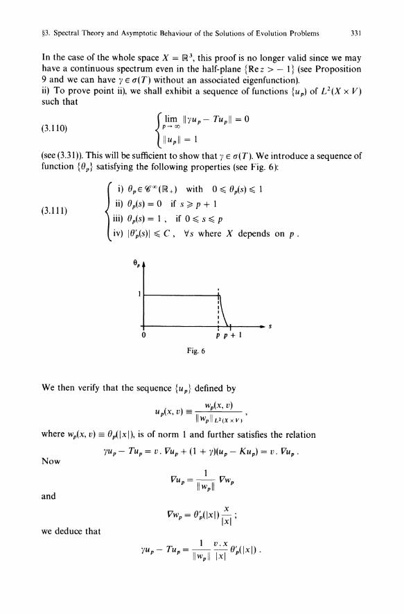
§3. Spectral Theory and Asymptotic Behaviour of the Solutions of Evolution Problems 331
In the case of the whole space X = 1R 3, this proof is no longer valid since we may have a continuous spectrum even in the half-plane {Re z > - 1} (see Proposition 9 and we can have y E /1(T) without an associated eigenfunction). ii) To prove point ii), we shall exhibit a sequence of functions {up) of U(X x V) such that
(3.110) p -+ 00 {lim Ilyu p - TUpl1 = 0
Ilupll = 1
(see (3.31)). This will be sufficient to show that y E /1(T). We introduce a sequence of function {Op} satisfying the following properties (see Fig. 6):
(3.111)
i) OpE CjCOO(IR+) with 0::::; Op(s)::::; 1
ii) Op(s) = 0 if s ~ p + 1
iii) Op(s) = 1, if 0::::; s::::; p
iv) I O~(s) I ::::; C, V s where X depends on p .
9,
+-------------~r-----.s pp+1 o
Fig. 6
We then verify that the sequence {up} defined by
_ Wp(x, v) up(x, v) = ,
II wpll L2(X x VI
where wp(x, v) == OP(lxl), is of norm 1 and further satisfies the relation
yup - Tup = v. Vup + (1 + y)(u p - Ku p) = v. Vup . Now
and
we deduce that
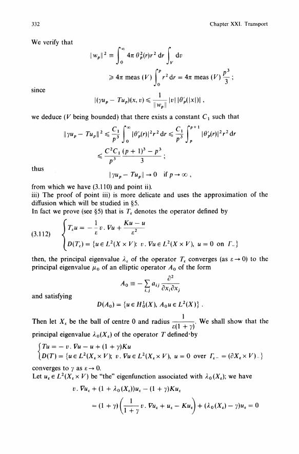
332 Chapter XXI. Transport
We verify that
fp p3 ~ 4n meas (V) 0 r2 dr = 4n meas (V) 3 ;
smce
I(Yu p - Tup)(x, v):::; II ~plllvlle~(lxl)1 ,
we deduce (V being bounded) that there exists a constant C 1 such that
Ilyu p- TUp112:::; C~ foole~(r)12r2dr:::; C~ fP+lle~(rWr2dr PoP P
C 2 C 1 (p + 1)3 _ p3 :::;-3- ;
p 3 thus
II yu p - Tu p II --+ 0 if p --+ 00 ,
from which we have (3.110) and point ii). iii) The proof of point iii) is more delicate and uses the approximation of the diffusion which will be studied in §5. In fact we prove (see §5) that is T. denotes the operator defined by
{T'U = _ ~ v. Vu + Ku -; u
(3.112) E E
D(T.) = {uEL2(XXV): V.VUEe(XXV), u=O on L}
then, the principal eigenvalue Ae of the operator Te converges (as E --+ 0) to the principal eigenvalue J10 of an elliptic operator Ao of the form
02
Ao == - Laij--i.j OXiOXj
and satisfying D(Ao) = {uEHMX), AoUEL2(X)}.
. 1 Then let Xe be the ball of centre 0 and radIUs . We shall show that the
£(1 + y) principal eigenvalue Ao(X.) of the operator T defined'by
{ Tu = - v. Vu - u + (1 + y)Ku D(T)= {UEe(X.X V); V. VUEL2(Xex V), u=O over r.- =(oXex V)_}
converges to y as E --+ O. Let u. E L 2(X. X V) be "the" eigenfunction associated with Ao (X.); we have
v. VUe + (1 + Ao (Xe))Ue - (1 + y)Ku.
= (1 + y) C : y v. VUe + u. - KU.) + (Ao (X.) - y)u. = 0
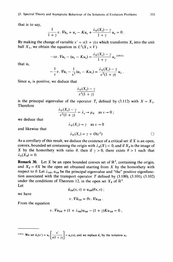
§3. Spectral Theory and Asymptotic Behaviour of the Solutions of Evolution Problems 333
that is to say, 1 Ao(X,) - y
-1 - v. VUE + u, - Ku, + 1 u, = 0 . + y + y
By making the change of variable x' = e(1 + y)x which transforms X, into the unit ball X b we obtain the equation in U(X I x V)
_ 1'7 _( -K )_Ao(X,)-y (161) ev. yU, u, U, - u, 1 + y
that is, 1 1 Ao(X,) - y
- - v. VUE - 2" (u, - Ku,) = 2(1 ) u,. e e e + y
Since u, is positive, we deduce that
AO(X,) - y e2 (l + y)
is the principal eigenvalue of the operator T, defined by (3.112) with X = X I' Therefore
we deduce that
and likewise that D
As a corollary of this result, we deduce the existence of a critical set: if X is an open, convex, bounded set containing the origin with Ao(X) < 0, and if Xo is the image of X by the homothety with ratio (J, then if y > 0, there exists (J > 1 such that Ao(Xo) = O.
Remark 30. Let X be an open bounded convex set of 1R 3 , containing the origin, and X 0 = (JX be the open set obtained starting from X by the homothety with respect to (J. Let Aoo, Uoo be the principal eigenvalue and "the" positive eigenfunction associated with the transport operator T defined by (3.100), (3.101), (3.102) under the conditions of Theorem 12, in the open set X 0 of IR 3.
Let Uoo(x, v) == uoo((Jx, v) ;
we have v. VUoo = (Jv. VUoo.
From the equation
v. VUoo + (1 + Aoo)Uoo - (1 + y)Kuoo = 0 ,
(161) We set ii,(X') = ", [_X_' -J = ",(X). and we replace ii, by the notation ",. e(l +)')
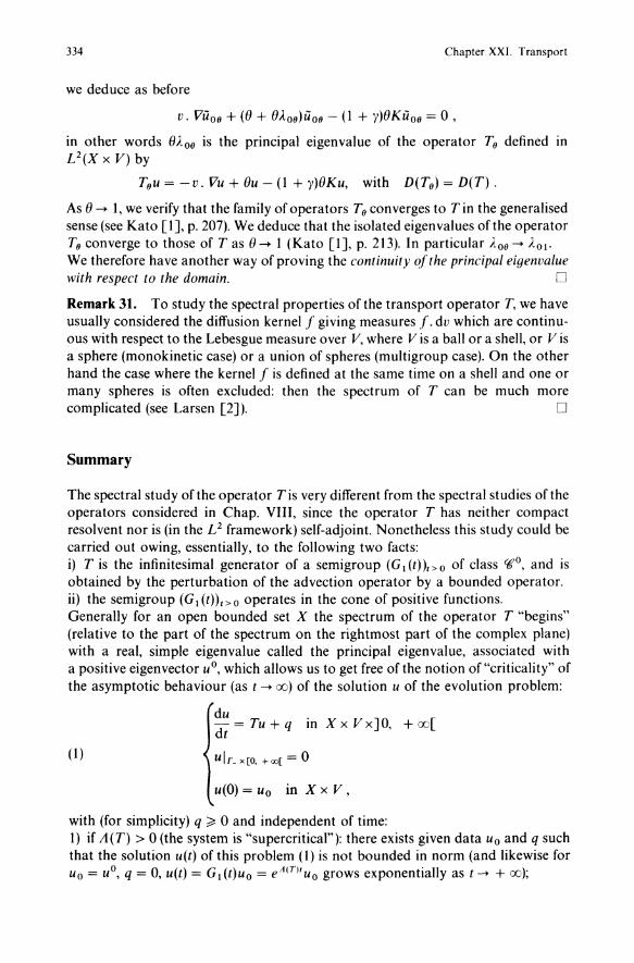
334 Chapter XXI. Transport
we deduce as before
v. VUoo + (8 + 8).00)uoo - (1 + y)8Kuoo = 0,
in other words 8).00 is the principal eigenvalue of the operator To defined in L2(X x V) by
Tou = -v. Vu + 8u - (1 + y)8Ku, with D(To) = D(T).
As 8 -> 1, we verify that the family of operators To converges to T in the generalised sense (see Kato [1], p. 207). We deduce that the isolated eigenvalues of the operator To con verge to those of T as f) -> 1 (Kato [1], p. 213). In particular ). 00 -> A 01'
We therefore have another way of proving the continuity o{the principal eigenvalue with respect to the domain. C
Remark 31. To study the spectral properties of the transport operator T, we have usually considered the diffusion kernel f giving measures f. dv which are continuous with respect to the Lebesgue measure over V, where V is a ball or a shell, or V is a sphere (monokinetic case) or a union of spheres (muItigroup case). On the other hand the case where the kernel f is defined at the same time on a shell and one or many spheres is often excluded: then the spectrum of T can be much more complicated (see Larsen [2]). 0
Summary
The spectral study of the operator T is very different from the spectral studies of the operators considered in Chap. VIII, since the operator T has neither compact resolvent nor is (in the L 2 framework) self-adjoint. Nonetheless this study could be carried out owing, essentially, to the following two facts: i) T is the infinitesimal generator of a semigroup (G dt) hoof class rca, and is obtained by the perturbation of the advection operator by a bounded operator. ii) the semigroup (Gdt))t>o operates in the cone of positive functions. Generally for an open bounded set X the spectrum of the operator T "begins" (relative to the part of the spectrum on the rightmost part of the complex plane) with a real, simple eigenvalue called the principal eigenvalue, associated with a positive eigenvector uO, which allows us to get free of the notion of "criticality" of the asymptotic behaviour (as t -> (0) of the solution u of the evolution problem:
du dt = Tu + q in X x V x] 0, + oo[
(1) UIL X [0, +oo[ = 0
u(O) = Uo in X x V ,
with (for simplicity) q ~ 0 and independent of time: 1) if A(T) > 0 (the system is "supercritical"): there exists given data Uo and q such that the solution u(t) of this problem (1) is not bounded in norm (and likewise for Uo = uO, q = 0, u(t) = G1(t)uo = eA(T)t uo grows exponentially as t -> + (0);
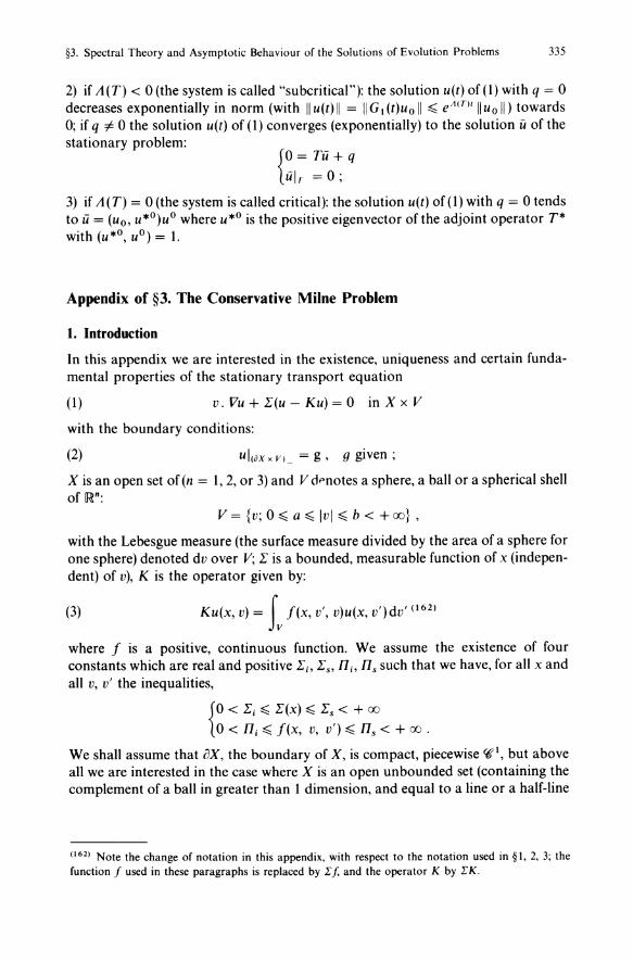
§3. Spectral Theory and Asymptotic Behaviour of the Solutions of Evolution Problems 335
2) if A(T) < 0 (the system is called "subcritical"): the solution u(t) of(1) with q = 0 decreases exponentially in norm (with II u(t) II = II G 1 (t)uo II ~ eA(T)t II Uo II) towards 0; if q #- 0 the solution u(t) of (I) converges (exponentially) to the solution Ii of the stationary problem:
{~ = Tii + q ul r = 0;
3) if A(T) = 0 (the system is called critical): the solution u(t) of (1) with q = 0 tends to ii = (uo, u*O)UO where u*o is the positive eigenvector of the adjoint operator T* with (u*o, UO) = l.
Appendix of §3. The Conservative Milne Problem
1. Introduction
In this appendix we are interested in the existence, uniqueness and certain fundamental properties of the stationary transport equation
(I) v. Vu + 1:(u - Ku) = 0 in X x V
with the boundary conditions:
(2) ul(oXx V) = g, g gIven;
X is an open set of(n = 1,2, or 3) and V d"'notes a sphere, a ball or a spherical shell of IR":
V = {v; 0 ~ a ~ Ivl ~ b < + <Xl} ,
with the Lebesgue measure (the surface measure divided by the area of a sphere for one sphere) denoted dv over V; 1: is a bounded, measurable function of x (independent) of v), K is the operator given by:
(3) Ku(x, v) = Iv f(x, v', v)u(x, v')dv' (162)
where f is a positive, continuous function. We assume the existence of four constants which are real and positive 1:;, 1:" fl;, fls such that we have, for all x and all v, v' the inequalities,
{o < 1:; ~ 1:(x) ~ 1:s < + CX)
0< fl; ~ f(x, v, v') ~ fls < + <Xl .
We shall assume that ax, the boundary of X, is compact, piecewise ~I, but above all we are interested in the case where X is an open unbounded set (containing the complement of a ball in greater than I dimension, and equal to a line or a half-line
(162) Note the change of notation in this appendix, with respect to the notation used in § 1, 2, 3; the function f used in these paragraphs is replaced by Ef, and the operator K by EK.
336 Chapter XXI. Transport
in one dimension). As before y(x) denotes the outward normal to X, and (aX x V)= L the set of points of (aX x V) where the velocity direction is inward:
(4) (aX x V)- = {(x, v) E ax x V; v(x). v < O} (163)
It follows from the Hille-Yosida theorem that the spectrum of the operator Tp(164)
defined by:
(5) D(Tp) = {u E U(X X V); v. Vu E U(X x V), UI«lXX V)_ = O}
(6) Tpu = -v. Vu -L(X)(1 - K)u,
is contained in the half-plane ReA. :::::; wp. On the other hand if gEL 00 «aX x V)_) there exists (see Bardos [1]) a function g (belonging to the spaces U(X x V)) satisfying the following relations:
(7) v. Vg E U(X X V), (ji(oXx V)_ = g.
Therefore the solution of the problem
AU + vVu + L(1 - K)u = 0, ul(i'xxv)_ = g
is equivalent to the resolution of:
(8) {AU - Tu = - Ag - v Vg - L(1 - K)g U E D(T) and u = U + g .
Such a step, based on the linearity of the equations and on the trace theorems is absolutely standard and is called, in certain physics texts, the principle of superposition. We deduce that problem (1), (2) (far as the existence and uniqueness is concerned) is easy if A does not belong to the spectrum of T and relatively difficult if A is a spectral val ue. We shall now assume that the function f satisfies the hypotheses
(9)
(10)
f(x, v, v') = f(x, v', v) V(v, V')E VX V
tf(x, v, v')dv' = 1, V(x, V)EX X V.
The symmetry in v and v' is realised in certain physical problems, particularly if f only depends on the scalar product of the vectors v and v'. The relation
(11) tf(X, v', v)dv' = 1
means that there are as many particles emitted by the medium as there are absorbed; it is for this reason that we speak of a conservative medium. This relation
(163) We shaH also use the notation
(iJXx V)+ = r+ = {(x,v)eiJXx V; v(x).v >O},
(164) We have also denoted this operator by Tand, where there is no risk of confusion, shaH continue to do so.
§3. Spectral Theory and Asymptotic Behaviour of the Solutions of Evolution Problems 337
has important consequences for the analysis of the operator Kx defined by:
(12) Kxu(v) = Lf(X, v, v')u(v')dv' .
Indeed Kx is a self-adjoint compact operator(t65) in L2(V). From relation (11) we deduce two choices: a) the norm of Kx is less than or equal to 1; b) 1 is an eigenvalue of Kx and the function v -+ 1 v is an eigenvector of Kx. This is therefore an eigenvalue of largest modulus. Further Kx is a positive operator. We therefore deduce from the Krein-Rutman theorem that 1 v is a simple eigenfunction(166) of Kx. The operator (I - K)(t67) therefore decomposes the space L2(V) into
(13) L 2 (V) = Ker (I - K) EB Ker (I - K).1 ;
the space Ker(I - K) coincides with the constants and the space Ker(I - K).1 coincides with the functions w(v) satisfying the relation:
(14) L w(v)dv = O.
Further, there exists a constant CXo > 0 (independent of x, from the continuity of f(x, v, v')) such that we have, for every function w(x, v) satisfying the relation
(15) LW(X,V)dV=O,
(16) L (w(x, v) - Lf(X, v, v')w(x, v')dv')w(x, v)dv ~ CXo L Iw(x, vWdv.
To see the difficulty of problem (I), (2) in the conservative case (this difficulty is due to the fact that A = 0 whether or not it is an eigenvalue of the transport operator) we prove the following theorem:
Theorem 1. We denote by Tp the transport operator defined in U(X x V) by (5) and (6). We assume that the functions 1: and f satisfy hypotheses (4), (9) and (10), corresponding to a conservative medium. Then:
i) For every p, 1 ~ p ~ + 00 the spectrum of Tp is contained in the half-plane ReA ~ O. ii) If X is bounded,for all p, 1 ~ p ~ + 00, 0 does not belong to the spectrum of Tp. iii) If X contains the complement of a ball (or in one dimension coincides with a half-line), for 1 ~ p < + 00, 0 belongs to the spectrum of Tp-
Proof Taking account of hypothesis (10) by using the Holder inequalities we see that Tp is an accretive operator in U(X x V) and point i) is obvious. It follows from
(165) Under the hypotheses indicated previously thatfis continuous over X x V x Vand V is bounded. (166) This is proved, for example, by the strong Krein-Rutman theorem in the space 'iIJ'(V). (167) We omit the index x of Kx to simplify notation
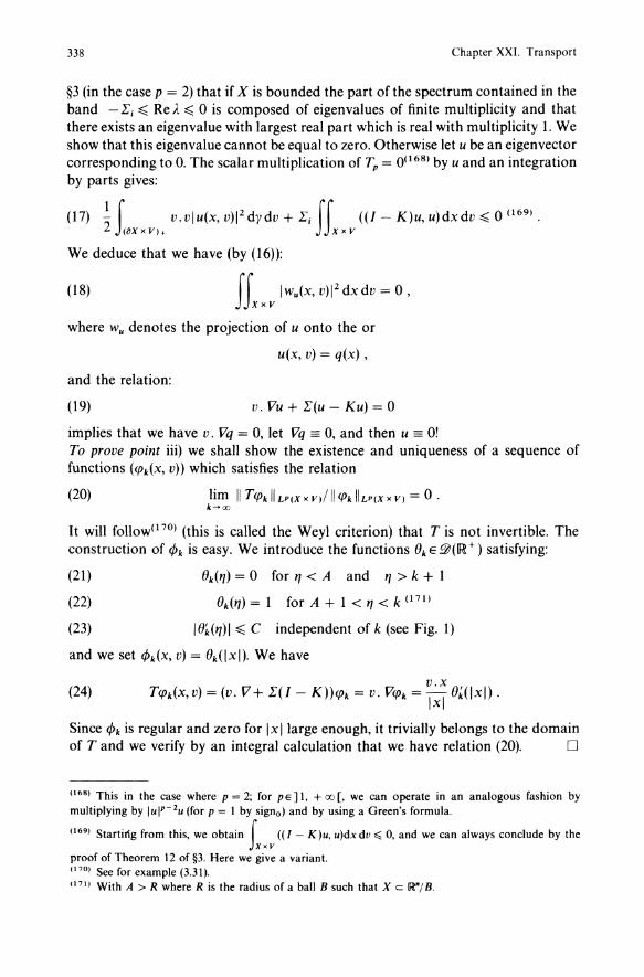
338 Chapter XXI. Transport
§3 (in the case p = 2) that if X is bounded the part of the spectrum contained in the band -1: i :!( Re A :!( 0 is composed of eigenvalues of finite multiplicity and that there exists an eigenvalue with largest real part which is real with multiplicity 1. We show that this eigenvalue cannot be equal to zero. Otherwise let u be an eigenvector corresponding to O. The scalar multiplication of Tp = 0(168) by u and an integration by parts gives:
(17) ~ r v.v I U(X,VW dYdv+1:i If «(I-K)u,u)dxdv:!(0(169). 2 JOJxxV)+ xxv
We deduce that we have (by (16)):
If Iwu(x, vWdxdv = 0, xxv
(18)
where Wu denotes the projection of u onto the or
u(x, v) = q(x) ,
and the relation:
(19) v. Vu + 1:(u - Ku) = 0
implies that we have v. Vq = 0, let Vq == 0, and then u == O! To prove point iii) we shall show the existence and uniqueness of a sequence of functions (CPk(X, v)) which satisfies the relation
(20)
It will follow(170) (this is called the Weyl criterion) that T is not invertible. The construction of 4h is easy. We introduce the functions 8k E !0(1R +) satisfying:
(21)
(22)
(23)
8k (l]) = 0 for I] < A and I] > k + 1
8k (l]) = 1 for A + 1 < I] < k (171)
18k(I])I:!( C independent of k (see Fig. 1)
and we set 4>k(X, v) = 8dlxl). We have
(24) v.x
Tcpdx, v) = (v. V + 1:(1 - K))CPk = V. Vcpk = -I 8~(lxl) . Ix
Since 4>k is regular and zero for Ixllarge enough, it trivially belongs to the domain of T and we verify by an integral calculation that we have relation (20). 0
(168) This in the case where p = 2; for pE] I, + 00 [, we can operate in an analogous fashion by multiplying by lul p - 2u (for p = I by signo) and by using a Green's formula.
(169) Starting from this, we obtain f ((1- K)u, u)dxdv,,; 0, and we can always conclude by the Xxv
proof of Theorem 12 of §3. Here we give a variant. (170) See for example (3.31). (171) With A > R where R is the radius of a ball B such that X c !R"/ B.
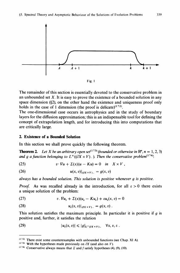
§3. Spectral Theory and Asymptotic Behaviour of the Solutions of Evolution Problems 339
A A+l k k + 1
Fig. 1
The remainder of this section is essentially devoted to the conservative problem in an unbounded set X. It is easy to prove the existence of a bounded solution in any space dimension (§2), on the other hand the existence and uniqueness proof only holds in the case of 1 dimension (the proof is delicatep 72).
The one-dimensional case occurs in astrophysics and in the study of boundary layers for the diffusion approximation; this is an indispensable tool for defining the concept of extrapolation length, and for introducing this into computations that are critically large.
2. Existence of a Bounded Solution
In this section we shall prove quickly the following theorem.
Theorem 2. Let X be an arbitrary open set(l73) (bounded or otherwise in [Rft, n = 1,2,3) and g a function belonging to L 00 ((aX x V)-). Then the conservative problern(l74):
(25)
(26)
v' Vu + I"(x)(u - Ku) = 0 in X x V,
u(x, v) I (oX x V)_ = g(x, v)
always has a bounded solution. This solution is positive whenever g is positive.
Proof As was recalled already in the introduction, for all e > 0 there exists a unique solution of the problem:
(27)
(28)
v. VUE + E(x)(u. - Ku.) + eu.(x, v) = 0
u.(x, v)l(oxXV)_ = g(x, v).
This solution satisfies the maximum principle. In particular it is positive if g is positive and, further, it satisfies the relation
(29)
(172) There exist some counterexamples with unbounded functions (see Chap. XI A). (173) With the hypotheses made previously on oX (and also on V). (174) Conservative always means that E and f satisfy hypotheses (4), (9), (10).
340 Chapter XXI. Transport
From (29), u, is uniformly bounded in L 00 (X x V). A weak-* passage to the limit in L 00 (X x V) then allows, taking account of the usual trace theorems, a passage to the limit as 6 tends to zero and we obtain relation (26). We therefore construct a bounded solution of (25), (26). 0
3. Uniqueness of the Bounded Solution (Case where X = [R+).
From now on we restrict ourselves to the one-dimensional case X = [R+ (which corresponds to the "physical" case of a half-space where X = [Rn - 1 X [R + with given data g, L, f independent of the first of n - 1 space variables Xl, ... , Xn - 1; then assuming that the unknown u is itself independent of Xl, ... , Xn - 1, we use for
. 1" h . ou sImp IClty t e notatIon Xn = x and v. V.u = Vn -. ox Further we denote: V+ = {VE V, Vn > O}, I VI = meas(V), and:
{<CP' cp') ~ <cp, cp')y = Iv cp(v)cp'(v)dv ,
(30)
<cp) = <cp, l)y = Iv cp(v) I~I' \lcp, cp' E U(V) ,
and also for every function 4J = 4J(x, v) with 4J(x, . ) E L 2( V)
< cp(x» = Iv cp(x, v) Id;1 .
We can then state:
Theorem 3. Under hypotheses (4), (9), (10), and with X = [R+,for all gELOO(V), there exists a unique solution u in L 00 ([0, + 00 [ x V) of problem:
{i) Vn :: + L(X)(U - Ku) = °
ii) u(O, v) = g(v), \Iv E V + .
(31)
Proof The existence follows directly from Theorem 2. It remains to prove the
uniqueness. Let u be a solution of (31); by a change of variable x' = f: L(¢)d¢, we
are reduced to the case L = 1. We set
(32) def
w(x, v) = u(x, v) - <u(x»
that is to say wEker(l- K)1.. Then equation (31)i) is written:
(33) ou
Vn ox + (w - Kw) = 0.
§3. Spectral Theory and Asymptotic Behaviour of the Solutions of Evolution Problems 341
By multiplying (33) by u, we obtain, after integration over V, and with (16):
1 a 2 2 -"2 ax <vnu ) = <w - Kw, w) ;:: eto<w (x» .
From which we deduce the inequality, for all x and Y E IR +:
(34)
Now since U is bounded, we deduce:
(35) 2eto foo <W2(X'» dx' ~ <vnu2(x» - lim inf < Vn u2(y) < + 00 x y- + 00
Therefore for all h > 0, as x --+ + 00 we have
1 fX+h [1 fX+h JI /2 h x <lw(~)I)d~~ h x <w2(~»d~ --+0,
1 fX+h that is, h x u(~, . )d~ --+ 0 in L I (V), or even:
1 fX+h 1 fX+h (36) h x u(~")d~--+h x <u(~»d~ ifx--++oo inLI(V).
On the other hand, starting from (33) we take:
a i}x <vnu) = 0,
then: (37)
and by using (36):
<Vnu(x» = <vnu(O», \t'XEIR+,
1 fX+h 1 fX+h <vnu(x» = h x <vnu(~» d~ = :~n;, h x <vnu(~» d~ = 0 .
Then we see that:
(38) <vn u2(x» = <vn)«U(X»)2 + 2<u(x» <vnu(x» + <vnw2(x»
= <vn w2 (x») .
Therefore from (35), there exists a sequence (xm), Xm --+ 00 such that:
<w2(xm» --+ 0,
therefore from (38):
342 Chapter XXI. Transport
By substituting this in (34) we obtain:
(vnu2(0) ~ 2IXo lim IX" (w2(x)dx. n~oo 0
Now if g = 0 we have:
(vnUZ(O) = t _ vnuZ(O)dv ~ 0 ,
which implies that w(x) = 0, 'fix.
We immediately deduce from this, by (33), that ~~ = 0 then u = O. o • Using the same techniques as above we can show (see Sentis [2]) that there exists Au E IR such that:
1 fX+h h X u(~,· )d~ -+ Au in Ll(V) if x -+ 00 .
• Besides, using other tools we can show that there exists IX > 0 (depending only on 1: and K) and constants C1(u) and C2 (u) such that:
(39) {IIU(X)- (u(x)llt2(V)~ C1(u)e- U
I(u(x) - Aul ~ Cz(u)e- U
(see Bardos-Santos-Sentis [1]). • For complementary results on this problem see §4 on the Chandrasekhar method.
4. Some Additional Properties Concerning the Solution of the Conservative Milne Problem
We thus consider the solution of the conservative Milne problem in 1R+x x V:
(40) Vn ~~ (x, v) + 1: (U(X, v) - tf(X, v, v')u(x, V')dV') = 0 in lR+x x V
(41) u(O, v) = g(v) for Vn > 0 .
As we have seen the solution of (40), (41) is unique and converges exponentially towards a limit denoted G(g) as x tends to infinity, (40), (41) defines a continuous linear mapping G from LOO(V+) into values in IR. We then have
Proposition 1 i) For all gEL oo(V+) we have:
(42)
ii) If g is positive then so is G(g). iii) We assume that f is independent of x and invariant by rotation, that is for every rotation R of V we have
(43) f(v, v') = f(Rv, Rv') .
§3. Spectral Theory and Asymptotic Behaviour of the Solutions of Evolution Problems 343
We denote by Dn(v) the solution of the problem:
(44) t Dn(v)dv = 0; Dn(v) - tf(V, v')Dn(v')dv' = Vn ;
then G(Dn) is positive(175).
Proof Points i) and ii) are obvious, it is sufficient to apply the maximum principle to the function u£ which is the solution of the problem
(45) {eo, + ". ~~ + l:(u, - Ku,) ~ 0, ;n
u.(O, v) = g(v) If vn > 0 ,
IR+ x V ,
and then to pass to the limit by letting e tend to zero. To prove point iii) we start by reducing to the case L == 1 by setting
(46) x' = J: L(s)ds
(we omit the symbol' in what follows). By multiplying the equation
(47) ou v - + u - Ku = 0 (176)
n ox
by x + Dn(v) and by integrating in x from 0 to infinity, and over v, it becomes
0= Iooo t Vn :~ '(x + Dn(v))dxdv + too t (1- K)u.(x + Dn(v))dxdv
Hence,
(48)
= t (vnu.(x + Dn(v))) 10 dv
+ t''' t[ -u(vnoox(X+ Dn(V)) + U.U-K)Dn(V)]dXdV (177)
+ G(Dn) t Dn(v)vndv - t VnU(O, v)Dn(v)dv
+ too t U( -Vn + (I - K)Dn(v))dv dx .
(175) Note that in the particular case where f is constant then D.(v) = v., and point ii) implies the positivity of G(D.). (176) We choose u with u(O, v) = D.(v) for v > O. (177) In the particular case where f is symmetric. The result remains true in the case where f is not symmetric, but the proof is more delicate.
344 Chapter XXI. Transport
Since f(v, v') satisfies the relations:
Ivf(V, v')dv' = 1, f(v, v') > 0,
we note (this occurs all the time in diffusion approximations) that we have:
(49) e ~f Iv vnDn(v)dv > O.
Therefore from relation (48) we deduce the formula:
(50) G(Dn) = + ~ f vn(u(O, v))Dn(v)dv . e v
From the symmetries of V and the relation (44), we have:
(51) h ~ f vn(Dn(v))2 dv = f (- vn)(Dn(v)f dv > 0 . v+ v_ We then deduce from (51):
(52) r vnu(O, v}Dn(v)dv = r vn(Dn(v))2dv + r vnu(O, v)Dn(v)dv Jv Jv+ Jv-
~h- Iv- (-vn)u(O,v)Dn(v)dv
~ hl/2 [h1/2 - (Iv _ (- vn)(u(O, v))2dv y/2 ] .
By multiplying the equation
au Vn ax + (J - K)u = °
by u and taking account of the asymptotic behaviour of u (see Sect. 3), we see that
I (x) = Iv vn(u(x, V))2 dv
is a decreasing function which tends towards zero as x tends to infinity. It follows that we have
(53) Iv vn(u(O, V))2 dv ~ 0 ,
so
(54) Iv + vn(Dn(v))2 dv ~ Iv _ (- vn)(u(O, V))2 dv .
This shows that the last term of (52) is positive. We have thus proved Proposition 1. o
§3. Spectral Theory and Asymptotic Behaviour of the Solutions of Evolution Problems 345
Remark 1. In the literature (Chandrasekhar [1], Case-Zweifel [1], Williams [1]), a certain number of calculations are to be found, concerning Milne's problem in the half-space, with constant coefficients:
(55)
(56)
au fl p. -;- (x, p.) + u(x, p.) - (1 + y) f(p., p.')u(x, p.')dp.' = 0 ux -1
in lR+x]-I,I[.
u(O, p.) = g(p.) if p. > 0 .
It is interesting to comment on these calculations in the light of some information given in this section.
(1) If y is negative, problem (55), (56) is subcritical and it has a unique square integrable solution(l78): as x tends to infinity this solution converges exponentially to zero. In fact we can prove the uniqueness of the solution not only in L 2(1R + x V) but in the class of tempered distributions (using duality). It follows that for y < 0 the problem
au fl p. -;- (x, p.) + u(x, v) - (1 + y) f(p., p.')u(x, p.')dp.' = 0 UX -1
(55)'
(56)' u(O, p.) = 0 if p. > 0
does not admit any solution which is a tempered distribution, in fact (and this does not contradict the fact that 0 does not belong to the spectrum of the linear operator associated with the homogeneous problem (55)', (56)'), it admits exponentially increasing solutions. It is not known whether this is always the case), but in explicit examples, for example with f(p., p.') = 1/2, these solutions are calculable by the method of "generalised" eigenfunctions of Case and Zweifel, or by the Wiener-Hopf method (see Chap. XI A), or by the invariant embedding method (see §4). This problem is interpreted by saying that the quantity u(O, p.) (p. > 0) represents the radiation from an infinitely large source at infinite distance. (2) The case y = 0 is the essential object of this appendix, we have seen that problem (55)" (56)' has a unique bounded solution, convergent to a constant as x -+ 00. The fact that this solution does not tend to zero as x -+ 00 is associated with the fact that 0 is the spectral radius of the associated homogeneous operator. In particular Vn is identified with p. and if f(p., p.') == 1/2, the function Dn(v) also coincides with p.. Therefore the extrapolation length(l79) is the limit, as x -+ 00, of the solution of the conservative Milne problem:
{p. ~: (x, p.) + u(x, p.) - ~ r 1 u(x, p.')dp.' = 0
(57)
u(O, p.) = p. if p. > 0 .
(178) If the given data 9 satisfies (see §4.3.2) J: Illg(IlW dll < + 00.
(179) For this concept, in a more general framework, see §5 at the end of Definition I.
346 Chapter XXI. Transport
This limit L can be calculated by the methods outlined above. It is equal to 0.7104. The fact that 0 belongs to the spectrum of the associated homogeneous problem is now indicated by the existence of a solution which is a tempered distribution, of:
(58) {
oii 1 I1 I" ax (x, 1") + ii(x, 1") -"2 -I ii(x, I"')dl'" = 0
ii(O, 1") = 0 if I" > 0 .
This solution is simply obtained by writing:
(59) ii(x, 1") = x - I" + u(x, 1")
where u(x, 1") denotes the solution of problem (57) (obvious). It increases linearly in X(IBO).
(3) The case y > 0 is often more singular; the resolution of the problem
(60) I" ~u (x, 1") + u(x, 1") - (1 + y) II /(1", I"')u(x, I"')dl'" = 0 uX -I
(61) u(O, 1") = g(l") for I" > 0
is not done, since 0 is then in the interior of the spectrum of the associated homogeneous operator. We have no existence or uniqueness results (in a class of distributions with suitable growth properties). The only results available concern the explicit homogeneous example:
(62) {
aU (1 + y) II , I" ax (x, 1") + u(x, 1") - -2- -I u(x, I" )dl'" = 0
u(O, 1") = 0 for I" > 0 .
By adapting the Chandrasekhar method we can show in this case the existence of solutions which oscillate as x -+ ClJ which corresponds to the fact that 0 is a point in the continuous spectrum. We can draw a "bifurcation" diagram for the solutions of (62) as a function of y.
y < 0 A unique solution; it grows exponentially; this is not a tempered distribution.
y = 0 A solution increasing in x; this is a tempered distribution
y > 0 An oscillating solution which is (obviously) a tempered distribution.
(180) For problem (58), see also Chap. XI A, §1.5.
§4. Explicit Examples 347
§4. Explicit Examples
1. The Stationary Transport Problem in the Whole Space IR
When we consider a medium filling the whole space ~3, which is homogeneous and subcritical, the monokinetic transport equation can be resolved explicitly for an arbitrary spatial and angular distribution of neutrons; the method of resolution (for example by Radon transformation) leads (as in the plane geometric case where the source of neutrons depends only on variables along a given direction) to the following problem in ~ x ] - 1, + 1 [: Find U = U(y, J.l) satisfying
au i fl (4.1) J.l oy(y,J.l)+L',U(y,J.l)=; -1 U(Y,J.l')dJ.L'+So(Y,J.l),YE~,J.lE[-I,I];
with So = So(y, J.l)(181) given; L', is the total uniform cross-section; is is the diffusion cross-section (and the shock law is assumed isotropic). By making the change of variable x = L',y and of function: u(x, J.l) = U(xlL'" J.l) we obtain the standard formulation: find u, the solution of
au C fl (4.2) J.l ox (x, J.l) + u(x, J.l) = 2 -1 u(x, J.l')dJ.L' + S(x, J.l), XE~, J.lE[ -1,1] ; (182)
with S(x, J.l) = So(Y, J.l)/L', given; c = islL', is the constant representing the average number of neutrons produced per collision. The spectrum of the operator T defined by
Tu(x, J.l) = -J.l :: (x, J.l) - u(x, J.l) + ~ f 1 u(x, J.l')dJ.L'
andD(T)={uEH;J.louloxEH} with H=L2(~x[-I,I]),
has been studied in §3.7; it is formed by the axis z = - 1 + i~ and by the segment [ -1, (c - 1)]; if we are in the subcritical case (c < 1), the spectrum is to the left of the real axis and problem (4.2) has a solution for all SEL2(1R x [-1,1]). We again solve this problem (4.2) (for c < 1 and for a source S which is a tempered
(181) So(Y, /1) represents the density of neutrons emitted per unit of space, of direction and of time by a volume source in y, in the direction /1 and therefore, with respect to the problem in [hl',
iY' i"' 2n dy d/1So(y, /1) is the number of neutrons per unit time, per unit surface (at right angles to the Yo lAO
axis of y) by the source between Yo and Yl in the conical domain (of revolution) with axis y and angle (with respect to this axis) 8 with cos 8 E [/10, /11]. (182) Compare with equation (3.66).
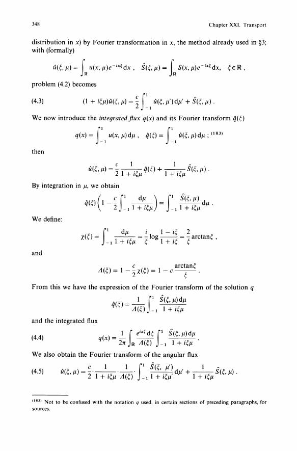
348 Chapter XXI. Transport
distribution in x) by Fourier transformation in x, the method already used in §3; with (formally)
u(~,J1)= I~u(x'J1)e-iX~dx, S(~,J1)= I~s(x'J1)e-iX~dx, ~EIR, problem (4.2) becomes
(4.3) C II -(1 + i~J1)u(~, J1) ="2 -I u(~, J1')dJ1' + S(~, J1) .
We now introduce the integrated flux q(x) and its Fourier transform 4(~)
q(x) = r I u(x, J1) dJ1, 4(~) = r I u(~, J1) dJ1 ; (183)
then
c 1 -u(~, J1) = "2 1 + i~J1 4(0 + 1 + i~J1 S(~, J1) .
By integration in J1, we obtain
4(~) (1 -.: II dJ1) = II S(~, J1) dJ1 . 2 _ I 1 + i~J1 - I 1 + i~J1
We define:
II dJ1 i 1 - i~ 2 X(O = 'j: = -log --'j: = ~ arctan~ ,
- I 1 + h,J1 ~ 1 + II, I,
and
c arctan~ A(~) = 1 - - X(O = 1 - c .
2 ~
From this we have the expression of the Fourier transform of the solution q
4(~) = _1_ II S(~, J1)dJ1 A(O -I 1 + i~J1
and the integrated flux
(4.4) 1 i eix~d~II S(~,J1)dJ1 q(x)=- -- . 21t ~ A(O -I 1 + i~J1
We also obtain the Fourier transform of the angular flux
A =.:. 1 ._1_. II S(~, J1'), 1 S (4.5) u(~, J1) 2 1 + i~J1 A(~) -I 1 + i~J1' dJ1 + 1 + i~J1 (~, J1) .
(183) Not to be confused with the notation q used, in certain sections of preceding paragraphs, for sources.
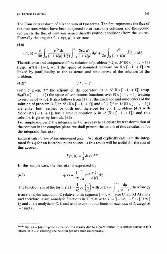
§4. Explicit Examples 349
The Fourier transform of u is the sum of two terms. The first represents the flux of the neutrons which have been subjected to at least one collision and the second represents the flux of neutrons issued directly (without collision) from the source. Formally the angular flux u(x, 11) is written:
(4.6)
c r ei~x d~ fl S(~, 11') , 1 r ei~x -u(x,ll) = 4njl<!(l + i~Il)A(~) -II + i~ll,dll + 2njl<!(1 + i~Il)S(~'Il)d~.
The existence and uniqueness of the solution of problem (4.2) in Sf" (IR x [ -1, + 1]) (resp . .,I(b(1R x [-1, + 1]) the space of bounded measure on IR x [ -1, + 1] are linked by (anti)duality to the existence and uniqueness of the solution of the problem:
(4.2)* T*u = S (with S given, T* the adjoint of the operator T) in 9'(1R x [ -1, + 1]) (resp. <6'o(1R x [ -1, + 1]) the space of continuous functions over IR x [-1, + 1] tending to zero as 1 X 1--+ ex)). It also follows from §3 that the existence and uniqueness of the solution of problem (4.2) in 9"(1R x [ -1, + 1]) and of (4.2)* in L2(1R x [ - 1, + 1]) are either both verified or both not: therefore for c < 1, problem (4.2) with SE9"(lRx[-I, +1]) has a unique solution u in 9"(lRx[-I, +1]), and this solution is given by formula (4.6). For simple sources S, the integrals in (4.6) are easy to calculate by transformation of the contour in the complex plane; we shall present the details of this calculation for the integrand flux q(x).
Explicit calculation of the integrated flux. We shall explicitly calculate the integrated flux q for an isotropic point source as this result will be useful for the rest of this account:
1 S(x, 11) = 2" c5(x) (184) •
In this simple case, the flux q(x) is expressed by
(4.7) q(x) = ~ r eix~ X(~) d~ . 4n jl<! A(~)
The function X is ofthe form X(O = ~ XI (i) with xdz) = f+ I ~; therefore XI I~ ~ - I 11 - z
is an s-analytic function in C relative to the segment [-1, + 1] (see Chap. XI A) and X and therefore A are s-analytic functions in C relative to L = ] - i CX), - i] u [i, i ex) [
(X and A are analytic in C/ L and tend to continuous limits on each side of L except at -i and i).
(184) sex, Jl) = 1b(x) represents the neutron density due to a point source (to a surface source in ~3) placed at x = 0, emitting one neutron per unit time isotropicaliy.
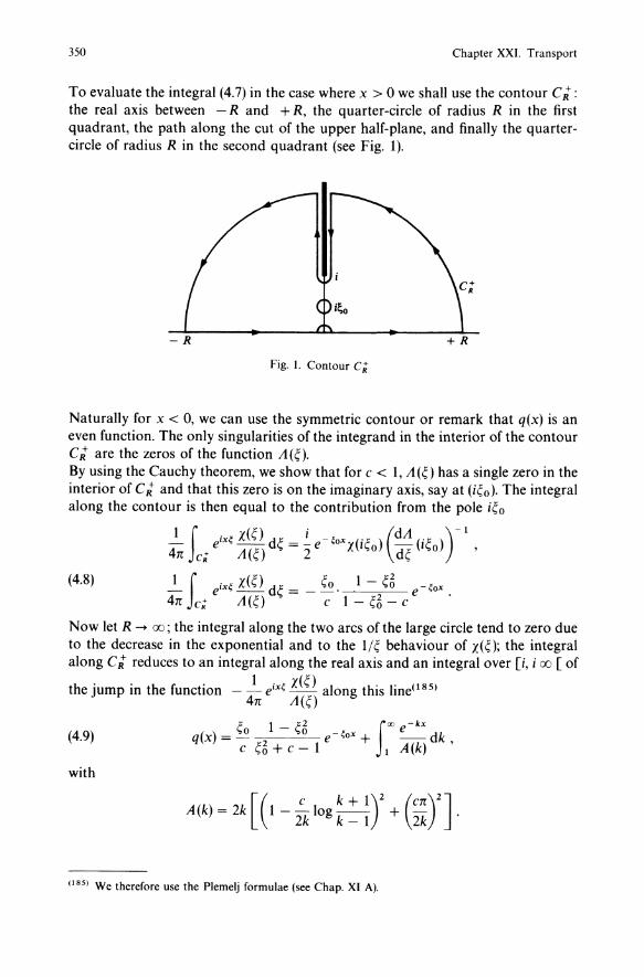
350 Chapter XXI. Transport
To evaluate the integral (4.7) in the case where x > 0 we shall use the contour Cit: the real axis between - Rand + R, the quarter-circle of radius R in the first quadrant, the path along the cut of the upper half-plane, and finally the quartercircle of radius R in the second quadrant (see Fig. 1).
Fig. 1. Contour c;
Naturally for x < 0, we can use the symmetric contour or remark that q(x) is an even function. The only singularities of the integrand in the interior of the contour Cit are the zeros of the function A(~). By using the Cauchy theorem, we show that for c < 1, A(~) has a single zero in the interior of Cit and that this zero is on the imaginary axis, say at (i~o). The integral along the contour is then equal to the contribution from the pole i~o
ix~ X '" dJ: _ 1 -~ox (.J: ) (.J: ) 1 i (J:). (dA )-1 4n e; e A(~) '" - "2 e X ''''0 d~ ''''0 ,
(4.8) ~ r eix~ X(~) d~ = _ ~o. 1 -2~5 e-~ox. 4n Je; A(e) c 1 - ~o - c
Now let R -+ 00; the integral along the two arcs of the large circle tend to zero due to the decrease in the exponential and to the 1/~ behaviour of X(~); the integral along Cit reduces to an integral along the real axis and an integral over [i, i 00 [ of
the jump in the function - 41n eix~ ~~~~ along this line(185)
_ ~o 1 - ~5 -~ox foo e- kx
(4.9) q(x) - ~ ~5 + c _ 1 e + 1 A(k) dk ,
with
[( c k + 1)2 (cn)2] A(k) = 2k 1 - 2k log k _ 1 + 2k .
(18S) We therefore use the Plemelj formulae (see Chap. XI A).
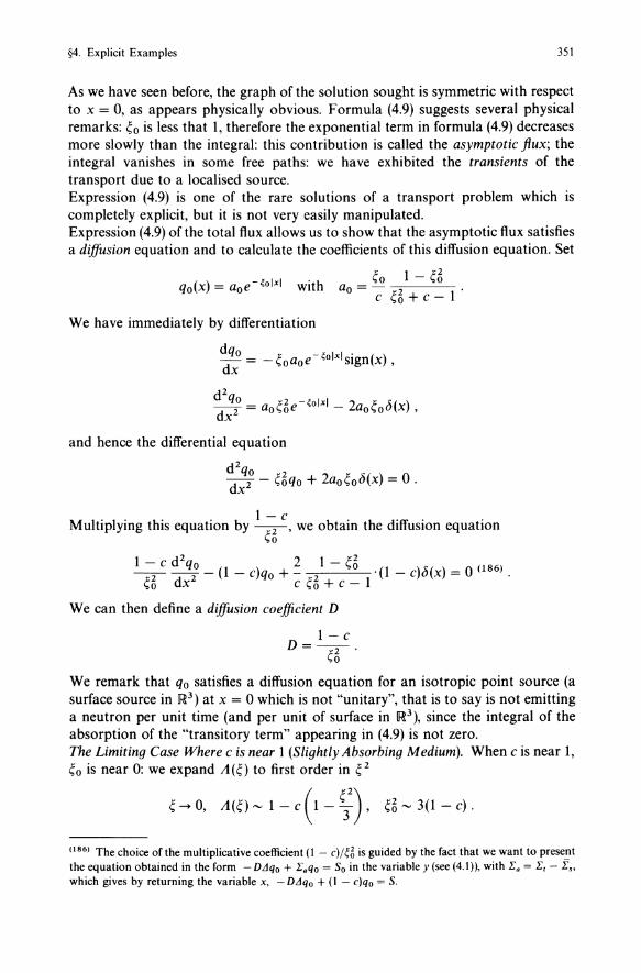
§4. Explicit Examples 351
As we have seen before, the graph of the solution sought is symmetric with respect to x = 0, as appears physically obvious. Formula (4.9) suggests several physical remarks: ~o is less that 1, therefore the exponential term in formula (4.9) decreases more slowly than the integral: this contribution is calIed the asymptotic flux; the integral vanishes in some free paths: we have exhibited the transients of the transport due to a localised source. Expression (4.9) is one of the rare solutions of a transport problem which is completely explicit, but it is not very easily manipulated. Expression (4.9) of the total flux alIows us to show that the asymptotic flux satisfies a diffusion equation and to calculate the coefficients of this diffusion equation. Set
~o 1 - a ao = - ;::2 + 1 . c ,,0 c-
with
We have immediately by differentiation
~~ = -~oaoe-~olxlsign(x),
d2q dx 2° = aoae-~olxl - 2ao~ob(x) ,
and hence the differential equation
d 2 qo 2 dx2 - ~oqo + 2ao~ob(x) = ° .
Multiplying this equation by 1 ~ c, we obtain the diffusion equation ~o
1 - C d2qo 2 1 - a ---- - (1 - c)qo + - .(1 - c)b(x) = 0(186). ~6 dx2 c ~6 + c - 1
We can then define a diffusion coefficient D
1 - c D=e;'
We remark that qo satisfies a diffusion equation for an isotropic point source (a surface source in [R3) at x = ° which is not "unitary", that is to say is not emitting a neutron per unit time (and per unit of surface in [R3), since the integral of the absorption of the "transitory term" appearing in (4.9) is not zero. The Limiting Case Where c is near 1 (Slightly Absorbing Medium). When c is near 1, ~ 0 is near 0: we expand A (~) to first order in ~ 2
~ --+ 0, A(~) - 1 - c (1 - ~32), ~6 - 3(1 - c) .
(186) The choice of the multiplicative coefficient (\ - c)/~~ is guided by the fact that we want to present the equation obtained in the form -D,1qo + Eaqo = So in the variable y (see (4.1)), with Ea = E, - f" which gives by returning the variable x, -D,1qo + (I - c)qo = S.
352 Chapter XXI. Transport
1 Therefore D ~ "3 (187), we recover the classical value of the diffusion coefficient and
the source term behaves like
2 1 - ~6 - 2 (1 - c) --+ 1 . c ~o + c - 1
At the limit of the slightly absorbing medium, we recover the classical diffusion equation.
Calculation of Angular Flux. The angular flux is expressed in integral form by equation (4.6); it can sustain the same treatment as the flux integral; we shall separate a transitory term and an asymptotic term. We make some remarks on its behaviour:
- The angular flux u(x, /1) for the direction /1, is discontinuous at x = 0, which is obvious by integration of the transport equation (then the integrated flux is continuous). - The angular flux is not bounded by /1 = O.
2. The Evolutionary Transport Problem in the Whole Space
The evolution problem for mono kinetic transport for a homogeneous medium occupying the whole space 1R 3 , without a source term (and for a given initial condition Vo only depending on the variable along a given direction(l88») reduces to the following problem (in V) in lRy x [ -1, + 1] x IRr+:
{av av L f+l Tr(Y,/1,r) + /1ay(Y,/1,r) + L I V(Y,/1,r) = c 21 -1 V(Y,/1',r)dlJ.'
V(y, /1, 0) = Vo(y, /1)
(with y E IR, /1 E [ - 1, + 1], r ~ 0); the parameters c and LI are positive. The changes of variable x = LlY, t = Llr and of unknown function
u(x, /1, t) = V (;/ /1, ~J, uo(x, /1) = Vo (;/ /1)
transforms the preceding problem into the "standard" form (in IRx x [-1, + 1] x IR:):
iii (x, p, t~+ P ax (x, p, tj + u(x, p, t) ~ '2 _. u(x, p', tjdp' {au au c f+ 1
u(x, /1, 0) - uo(x, /1) .
(187) Recall that we taken 1:,-1 as our unit of length. Returning to the units of formula (4.1) we have D = 1/(31:,) (see Bussac-Reuss [1]). (188) Or even in the case of an arbitrary initial condition, by Radon transformatIOn.
§4. Explicit Examples 353
The study of the asymptotic behaviour as t -+ + 00 of the solution of this problem was looked at in §3. We intend to repeat this study here in the case where the initial condition is of the form:
Uo(X, Ji) = cPo(Ji)eikx
(with k > 0 and cPo given with, for example, cPo Holder continuous of order rx, 0< rx < 1) by using the Laplace transformation in t, and with explicit formulae. The solution of the proposed problem is then sought in the form:
u(x,Ji, t) = cP(Ji, t)eikx ,
and cP must be the solution of the Cauchy problem in [ -1, + 1] x ~I+:
{
DcP Cf+1 at (Ji, t) + (1 + ikJi)cP(Ji, t) = 2 -I cP(l1', t)dJi'
cP(Ji, 0) = cPo(Ji) .
We now apply the Laplace transformation(189) with respect to t and denote by $ the Laplace transform of cP:
$(Ji, s) = Loc e-S1cP(Ji, t)dt .
We then obtain the equation for $(Ji, s):
(4.10) (1 + s + ikJi)$(Ji, s) = ~ fl $(Ji', s)dJi' + cPo(Ji) . 2 -I
Expression (4.10) is analogous to (4.3) and is resolved in an identical manner. Set
$(s) = fl $(11', s)dl1' ; -I
f+ I
$ is the Laplace transform of the integrated flux cP, with cP(t) = _ I cP(Ji, t) dJi.
Then
By defining
and
A(s) = 1 - ~ fl dJi 2 _ I 1 + s + ikJi '
(189) See Chap. XVI.
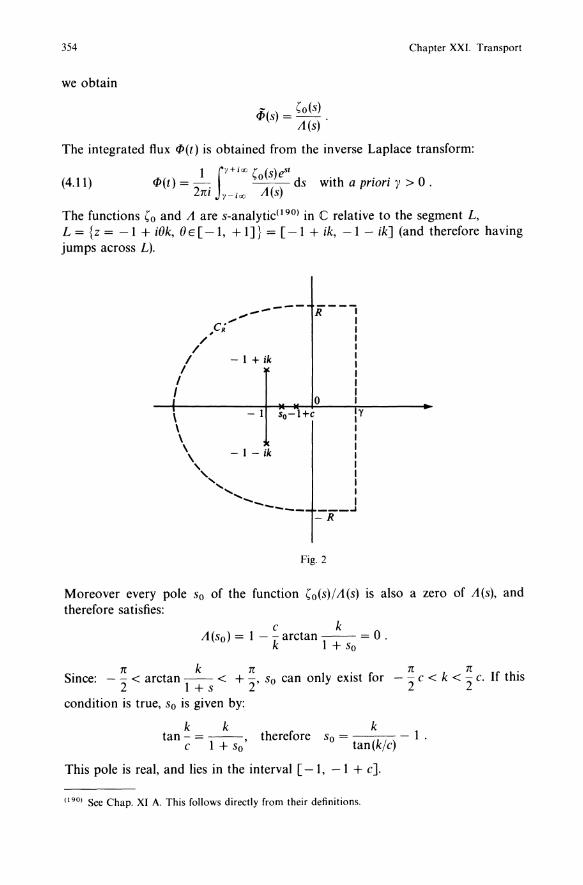
354 Chapter XXI. Transport
we obtain
qJ(S) = (0(5) . A(s)
The integrated flux (/J(t) is obtained from the inverse Laplace transform:
(4.11) 1 fY+ iOO ( (s)eSI
(/J(t) = -2 . _0 __ ds with a priori y > 0 . m y-ioo A(s)
The functions (0 and A are s-analyticC190) in C relative to the segment L, L = {z = -1 + iOk, BE[-I, +1]} = [-1 + ik, -1- ik] (and therefore having jumps across L).
/ I
/ I I
/ c'''' , R
",-.... ---
- 1 + ik
R--' I I I I I I I I I I
,Y I I I I I I I I I ___ ..J
-R
Fig. 2
Moreover every pole So of the function (o(s)/A(s) IS also a zero of A(s), and therefore satisfies:
c k A(so) = 1 - -k arctan -- = 0 .
1 + So
. n k n I. .. Smce: - - < arctan -- < + -, So can on y eXist lor 2 1 + s 2
condition is true, So is given by:
n n . - - c < k < - c. If thiS
2 2
k k tan-=--
c 1 + so'
k therefore So = tan(k/c) - 1 .
This pole is real, and lies in the interval [ - 1, - 1 + c].
(190) See Chap. XI A. This follows directly from their definitions.
§4. Explicit Examples 355
To evaluate <1>(t) from (4.l1), we use a "closed" contour C R in the left complex half-plane, with R --+ co; we therefore find that <1>(t) is of the form:
1 f- I + ik [, (S)J <1>(t) = <1>1(t) + <1>2(t) with <1>dt)=-2 . ~() estds, 11:1 -I-ik As L
( where ['o«s»J denotes the jump in the function 'o(s) across L) and with <1>2 (t) A s L A(s)
denoting, in the case where Ik/cl < ~, the contribution due to the pole so, that is:
{ ( dA )-1
((so) ds(so) esot if Ik/cl < ~ <1>2(t) =
o if Ik/cl >~ .
The determination of the function <1>(t) ("the integrated flux") allows us then to obtain the function <1>(fl, t) (and consequently, of u(x, fl, t) and U(y, fl, r» by:
<1>(fl, t) = ~ f~ <1>(s)e(1 +ikll)(s-t)ds + <1>o(fl)e-(1 +ikll)t .
The study of the asymptotic behaviour of <1>(t) (and therefore of <1>(fl, t» as t --+ + 00 is easily deduced from these formula.
i) Ikl < c~. The "transitory" term <1>1 (t) tends to zero more quickly than esot as t --+ + co. The dominant term, for large enough t, is therefore <1>2(t) which gives an exponential asymptotic decrease (in esot ) as t --+ co.
ii)lkl>c~. Then <1>2 (t) = 0 and the asymptotic behaviour of <1>(t) as t --+ co is that of <1>dt).
3. The Stationary Transport Problem in the Half-Space by the Method of "Invariant Embedding"
3.1. Introduction
The treatment of the half-space allows a first approach to the study of the neutron flux in the neighbourhood of a surface which does not reflect any free neutrons(191). This problem can be treated analytically by numerous methods; historically this problem was solved for the first time by Wiener-Hopf factorisation(192). It is also easily solved by the method of singular eigenfunctions( 193), but we shall present the
(191) A condition which we have called the absorbing boundary condition in §2 and §3. (192) See Chap. XI A, §1.5 in the case of a zero entrant flux. (193) See below.
356 Chapter XXI. Transport
resolution by "invariant embedding" which, apart from being interesting in its own right, has generalisations to the plate problem. The solution of this problem, called in astrophysics, Milne's problem allows us to calculate the emergent angular flux and to introduce the extrapolation length( 194) which is very generally used in applications. This problem is also solved in a slightly more general framework in Sentis [2].
3.2. The Milne Problem with Imposed (Nonzero) Incoming Neutron Flux
The Milne problem leads to solving the system (see introduction to §3.6)
(4.12) x 2 -I {i) Ji:U(X'Ji)+U(X'Ji)=~fl u(x,Ji')dJi', XE~_, JiE[-I,I],
ii) u(O, Ji) = g(Ji) , Ji E [ -1, 0]
where g(Ji) is a given positive function representing the flux of neutrons incident on the surface of a semi-infinite medium. From §3, the spectrum of the operator T defined in H = L 2 (] - 00, ° [ x [ - 1, 1]) by
{i) D(T)={UEH; Ji::EH, U(O,Ji) = ° if JiE[-I'O]} ,
(4.13) a fl ii) Tu(x, Ji) = - Ji a: (x, Ji) - u(x, Ji) + ~ _ I u(x, Ji') dJi', U E D( T) ,
comprises the interval [ -1, c - 1] of the complex plane (see §3, Proposition 11). Problem (4.12) with 9 = ° does not have a nonzero solution in H(195) when c is greater than 1 (the semi-infinite medium is then supercritical and problem (4.12)
with 9 =P ° [r 1 IJillg(JiW dJi < + 00 ] no longer. has a physical sense and does
not necessarily admit a solution in H), see Weinberg and Wigner [1]. To show the existence of the solution of (4.12) when c < 1, we use a lifting of the given function g:
(4.14) {e-X/llg(Ji) if Ji< 0,
w(x, Ji) = ° 'f ° 1 Ji > .
We verify that if g(Ji) is such that r I IJillg(JiW dJi < + 00, then WE W 2 , with:
W2 = {U E H: Ji :: E H}. Set
(4.15) U=u+W;
(194) This will also be seen in §5. (195) Or more generally in U(IIL x [-1, + 1]), pE [1, + OCJ [. This implies that T does not have an eigenvector in these spaces.
§4. Explicit Examples 357
problem (4.12) is equivalent to: find ii E D(T) satisfying
(4.16) Tii=J with J(X,Ji) = -~rl w(x,Ji')dJi'.
This problem has a solution ii when c < 1 because 0 ¢a(T)(196). In the case c = 1 Theorem 4 of §2 does not apply since 0 E a(T) and the problem cannot have a solution in H (that is, in L 2 ): and indeed it has none, by the result given before in Theorem 3 of the appendix of§3 (see also Bardos-Sentis-Sentos [1] and Bensoussan-Lions-Papanicolaou [1]). 0
3.3. The Construction of Invariant Embedding and the Albedo Problem
In the case of problem (4.12) for the semi-infinite medium (with c < 1), the invariant embedding technique is particularly well adapted to the determination of the flux of outward neutrons induced by the flux of inward neutrons, this method is based on the fact that if we are on the x-axis, the medium "to the left" is also a semiinfinite medium from which we have a particular form of in variance by translation. We consider here the Milne problem in the framework of Ufunctions, p E [1, + 00 [
as in §2, the case p = 1 being particularly interesting from the physical point of view. The space
WP(IILx[-I, +1])= {UEU(IILX(-I, +1))'Ji::EU(II~LX[-I, +1])}
presents here the following particular trace property (see appendix of §2 or Cessenat [1]): the trace mapping: u E WP(IIL x [ -1, + 1]) -+ u(O, Ji)E U« -I, + I), is continuous and surjective for p E [1, + 00 [.
Moreover, for every c < 1, and every gEU(]-I,O[, IJildJi), problem (4.12) has a unique solution UE WP(IIL x [ -1, + I]), and the mapping g -+ U is linear and continuous from U(]-I,O[, IJildJi) into WP(IIL x[ -1, +1]). It follows, with the help of the trace theorem, that the mapping 9\~p): g -+ g with g(Ji) = u(O, Ji) for 0 ~ Ji ~ 1 is linear and continuous from U(] - 1,0 [, I Jil dJi) into U(]O, 1 [, JidJi). We are often interested in finding the function g directly (without calculating the function u) and therefore in knowing the operator 9\ = 9\~P), or even its kernel 9\(Ji, Ji') = 9\~P)(Ji, Ji'). We shall now do this. Note first of all that problem (4.12) with the boundary condition u(O, Ji) = g(Ji) for Ji E [0, 1] is ill-posed, and therefore that the operator 9\ does not have a continuous inverse. Besides, note too that the operator 9\ is "invariant under translation", in the following sense
(4.17)
for every solution u of the Milne problem (4.12) with g E U(] -I, 0[, JidJi).
(196) See Theorem 4 of §2, and also Proposition 5 of §2 in the setting L 1 (~_ X [ - 1, + I]), if gEL1(]-I,OLIJlldJl).
358 Chapter XXI. Transport
Indeed by setting u(x, J1) = u(x + xo, J1), u(xo, J1) = go(J1), J1 < 0, we see that u is the solution of (4.12) for the given data go on [ -1,0], and therefore
9{go = go = ui{ojx[o, 1) = ui{xojx[O, 1)'
We define, on IlL x [0, 1], the functions u+ and u- by:
(4.18) u + (x, J1) = u(x, J1), u - (x, J1) = u(x, - J1) ,
The transport equation (4.12)i) is then written, with the unknowns u+ and u-:
(4.19)
In general, the spaces U(]O, 1 [, dJ1) are preferred to the spaces U(]O, 1[, J1dJ1), and we therefore replace the operator 9{ = 9{?) by an operator denoted R = R~p) acting in U(]O, l[,dJ1), In the case where p = 1, we write:
(4,20)
J1U + (0, J1) = f R(J1, J1')J1'U - (0, J1')dJ1' (197) with J1U + and J1U - EL I (] 0, 1 [, dJ1)
and from (4.17), we also have, for every x ~ 0:
To determine R(J1, J1'), the following system of three equations is available:
with ° < J1 < 1 and x < 0, We differentiate the first relation with respect to x:
ou+ II ou-J1 ax (x, J1) = ° R(J1, A) ox (x, A)AdA ,
§4. Explicit Examples 359
a -We replace A ~ (x, A) by its value from the third equation:
11 a;: (x, 11) = f: dAR(Il, A)
x [U-(X, A) - ~ f: dll'(U-(X, 11') +;, r R(Il', v)u-(x, V)VdV)] = ° Finally we use this expression in the third equation to eliminate u+:
~ e R(Il, A)U- (x, A)AdA + e dAR(Il, A) 11 Jo Jo
X[U-(X'A)-~r dl1'(U-(X,Il')+;' r R(Il',V)U-(X,V)VdV)]
-~ f: dll' (U- (x, 11') +;, r R(Il', A)U- (x, A)AdA) = ° , which is, by simplifying: r dUu- (x, A) G + D R(Il, A) = ~ J: dll' (u- (x, 11') +;, r R(I1', v)u- (x, V)VdV)
x (1 + f: R(Il, A) dA) .
Since this relation is valid for arbitrary U - (x, A), we obtain:
(1 1) c (e ) ( 1 e R(A 1l')dA) (4.22) ~ + Ii R(Il, 11') ="2 1 + Jo R(Il, A)dA Ii + Jo ' A .
Finally, we set
(4.23)
which gives for 11 and 11' E [0, 1]
(4.24) G+;,)S(Il'Il')=~(1 + r S(Il, A) dAA) (1 + r S(A,Il,)dAA).
This relation shows the symmetry of the kernel: S(Il, 11') = S(Il', 11)· We now introduce the Chandrasekhar function H [1], defined by
(4.25) H(Il) = 1 + S(A,Il)~' IlE[O, 1]. 11 d"
o A
We then obtain the fundamental relation
(4.26)
360 Chapter XXI. Transport
and the function H(It) satisfies the nonlinear integral equation
H( ) = I + ~ H( ) fl H(It')dlt' It 21t It + ' o It It
(4.27)
Chandrasekhar showed the existence of the function H and its expression starting from the Wiener-Hopf factorisation(l98); this function, which depends on c, can easily be calculated numerically (by using a numerical integration procedure and one iteration)(199). Knowing the function H(It) we can immediately obtain the outgoing angular flux, at the point x = 0:
+(0 )=~H( )fIH(It')/!'g(-It')d/!' u ,It 2 It +" o It It
(4.28) o :;:; It :;:; 1 .(200)
Finding u+ (0, It) when we know g(lt) is called the Albedo problem. Application to the Milne problem with "sources at infinity" and zero incoming flux: We consider the following problem in the half space IR.
{
au C fl i) It-a (x,It)+u(x,It)=- u(x,/!,)dlt', xEIR_, ItE[-I,I]
x 2 _I
(4.29) ii) with the boundary condition u(O, It) = 0 for It E [ - 1, 0] ;
we further assume that c < 1 so that the only solution of this problem in U(IR_ x [ - 1, + 1]) is zero. We are interested in solutions which are not in U(IR _ x [ - I, + 1]) but increase exponentially as x -> - 00: these solutions represent the behaviour of the neutron flux in the neighbourhood of a nonreflecting surface(20 I) and far from "sources" (which will here be "localised" at - (0). We shall study some solutions of (4.29)i) having the asymptotic behaviour
e- kx
w(x,lt) = I _ kit' xEIR_, ItE[ -1, +1].
where k is a positive constant to be determined. For w to satisfy the transport equation (4.29)i), we must have
(4.30) c l+k
1 - 2k log 1 _ k = 0 .
This relation is the characteristic equation defining the fundamental spatial modes, which was already seen in Sect. 1: there exists a positive unique solution ko for 0< c < 1 (and this solution satisfies ko < 1).
(198) See Chap. XI A. (199) See Chandrasekhar [1]. (200) With the help of the properties of the function H we can verify that the mapping R = R,: Ilg( - Il) - IlU+ (0, Il) operating in L 1 (JO, 1 [, dll) is an integral operator (which justifies a posteriori the equation (4.20)), conserving the positivity and tending to a limit as c - 1 (which justifies its use as c = 1). (201) This is what the absorbing condition expresses.
§4. Explicit Examples
We look for u, the solution of the problem (4.29), in the form
u(x, J1) = u(x, J1) + w(x, J1) ,
where u satisfies the transport equation
au c I' J1 ax (X,J1)+U(X,J1)=2 _, u(x,J1')dJ1', XEIIL, J1E(-1, +1),
with the boundary condition
_ 1 u(O,J1) = -w(O,J1) = - , J1E(-I,O).
1 - koJ1
361
We transform the problem of "sources at infinity" to an Albedo problem which has been solved before; we have
_+ c r' H(J1')J1' dJ1' u (0, J1) = - 2 H(J1) Jo (J1 + J1')(1 + koJ1') , J1E(O, 1),
so finally, the solution of problem (4.29) at point 0, for J1 E] 0, 1 [, is:
To simplify this relation we note that:
1 1 (1 ko) (J1 + J1')(1 + koJ1') = 1 - koJ1 J1 + J1' - 1 + koJ1'
and we obtain
Now, we have
and
~ H( ) I' H(J1')koJ1' d '= ~ H( ) [I' H( ')d '- I' H(J1')d J1'] . 2 J1 0 1 + ko J1' J1 2 J1 0 J1 J1 0 1 + ko J1'
If for 11k> 1, we define H(1lk) by
H(1lk) = 1 + - H(1/k) J1 J1 c I' H( ')d ' 2k 0 (ilk) + J1' '
362 Chapter XXI. Transport
the preceding expression is written (since ko < 1)
c f' H(p')kop' c f' (1 ) 2: H(p) 0 1 + kop' dp' = 2: H(p) 0 H(p')dP' - H(p) 1 - H(ljko) .
Finally, the outgoing angular flux at the point x = 0 is
(4.31 ) u+(O ) - 1 x H(p) ,p - 1 - kop H(ljko)'
where ko is the solution of (4.30). This relation gives a simple physical significance to the function H(p), it is the emergent angular flux in the case of a "source at infinity",(up to a factor of [(1 - kop)' H(ljko)r')· Another application: The reduction of the transport problem in the whole space with two different media to a problem (with reflection) in the half-space. Assume that the whole space 1R3 is filled by two different media separated by the plane x = 0, medium (1) in IR~ being homogeneous and isotropic, and characterised (with the notation of (1.3)) by the constants 17, and f" while medium (2) in IR~ is characterised by 172 and f2 which only depend on the variable x (hence 172 = 172 (x, p) andf2 = f2(X, p, p')). We consider the stationary monokinetic transport problem (Ivl = 1) in 1R3 x S2:
Tu = 0,
or more generally Tu = q with q a given source with support in IR~ x S2 dependent only on the variable x (therefore q = q(x, p)), with T the "usual" transport operator (see (l.13)) with coefficients 17 and f defined by:
From the hypotheses made, the problem III 1R3 x S2 reduces to the following problem in IR x [ - 1, + 1]
Tu = 0 (or Tu = q)
with TI~Lx[-I. +1] = T" TI~+x[-I, +1] = T2 ;
since the operator T, is defined (by changing the variable 17, and f, to 17, = 1 and f2 = cj2) in IR_ x [ -1, + 1], by:
au, c f+' " T,u,(x,p) = -P-ax-(x,p)-u d x,p)+2: _, udx,p)dp
and the operator T2 in IR + x [ -1, + 1], by:
T2U2(X, p) = -p aaU2 (x, p) - (172 u2)(x, /l) + f+' f2(X, /l, P')U2(X, /l')dP' . x _,
We assume that 172 and f2 are positive and bounded, that c < 1 (medium (1) is subcritical) and that qEL'(IR+ x [-1, + 1]).
§4. Explicit Examples 363
Then, setting u = (Ub U2) with ul rr,L x [-1, + 1] = U1, U I~+ x [-1, + 1] = U2, the problem in u becomes the fol1owing transmission problem: Find (U1' uz) satisfying:
{ T1U1 = ° T2U2=0 or q
U1(0, J.l) = U2(0, J.l)
III ilL x [ -1, + 1]
III IR+ x [ -1, + 1]
for J.lE[ -1, +1] .
In the medium (1) the problem can be solved starting from the known function 9 on [-1,0] with g(J.l)=U1(0,J.l), -1~J.l~0 (with gEL1(]-1,0[, 1J.lldJ.l) for U E W1(1R x [ -1, + 1]), and udO, J.l) for J.l > ° is then given by u11 {OJ x [O.IJ = 91g, or again with the notation of (4.20):
J.lui(O, J.l) = r R(J.l, J.l')J.l'ul(O, J.l')dJ.l'
(for ul (0, J.l) = U1 (0, - J.l)). Finally the transmission problems reduces to a reflection problem in medium (2): find U 2 EL1(1R+ x [ -1, + 1]) the solution of:
{ i) T2u2=0(orq) in lR+x[-1,+1]
ii) u21{ojx(O.1) = 91(U21{o)X(-1.0») ,
condition ii) is also written:
J.lU2(0, J.l) = 11 R(J.l, J.l')J.l'U2(0, -J.l')dJ.l' = - fO R(J.l, -J.l')J.l'U2(0, J.l')dJ.l' , o -1
where the kernel R(J.l, J.l') is given by (4.23) and (4.26).
4. Case's(202) Method of "Generalised Eigenfunctions". Application to the Critical Dimension in the Case of a Band
D
We shal1 restrict ourselves to the case of an infinite homogeneous medium and consider the transport equation
au c f1 (4.32) J.l ax (x,J.l)+u(x,J.l)=2, _lu(x,J.l')dJ.l', xEIR, J.lE[-1,+1].
The eigenfunction approach is suggested by the classical method for the resolution of differential equations where we expand the solution in eigenmodes: the invariance under translation suggests looking for solutions in the form:
(4.33)
(202) See Case [1], Case-Zweifel [1].
364 Chapter XXI. Transport
By substituting in (4.32) and after division by 'l'(x)cP(f.1) this becomes
--=--+-- cP(f.1)df.1. 1 dt/J 1 C fl " t/J(x) dx f.1 2f.1cP(f.1) -I
These two expressions must be equal to a constant which we set to be -l/v; from which
1 dt/J ----t/J(x) dx v
and
(4.34)
Since this equation is linear and homogeneous, the normalisation is arbitrary; for simplicity we choose:
This problem (4.34) does not have a solution for every value of v: we shall determine v for the solution to exist. With the normalisation condition and after multiplication of(4.34) by v, it becomes
(4.34)'
This problem is not as easy as it would seem if we were restricted to classical solutions: it also admits solutions in the space of distributions, which are generalised eigenfunctions of Case(203). We examine two cases according to the values of v. Case 1: v ~[-1, 1]. Set
(4.35) cv
cPv(f.1) = 2(v - f.1)
The denominator does not vanish for f.1 E [ - 1, 1]; the normalisation condition leads to the equation
(4.36) A(v) = 0
where A is the function defined by
(4.37)
(203) See Case [\].
{
cv v + 1 A(v) = 1 - -log--
2 v-I 1 .
A(v) = 1 - cvtanh-l~
§4. Explicit Examples 365
(Note that we have previously encountered this expression - up to a change of variable). The function v -> A(v) is analytic in the complex plane cut along the segment [ _1,1]<204); (we take the principal defintion of the logarithm to define this function). Equation (4.36) has, depending on c < 1 or c > 1 two roots ± Vo which are real or purely imaginary corresponding to resonances for problem (4.32), (4.33). We denote the solutions of (4.32) thus obained by:
(4.38)
Case 2: v E [ - 1, 1].
We can then add to the solution of (4.34), the distribution A(V)t5(fl - v) where b is the Dirac distribution and A is a real parameter depending on v (see also §3.7). We shall therefore choose the solution in the form
cv 1 cPv(fl) = -2 pv -- + A(v)b(fl - v), fl E] -1, + 1 [
V-fl (4.39)
where pv denotes the Cauchy principal value; the normalisation condition leads to
{
A(V) = 1 _ cv pv II ~ = 1 _ cv log 1 + v 2 -IV-fl 2 I-v
(4.40)
A(V) = 1 - cvtanh- I v
Thus an "eigendistribution" of the transport operator can be associated to every v in the segment] -1, + 1 [ . The fundamental result due to Case and Zweifel(205) is that every sufficiently regular function v(x, fl) can be written in the form
(4.41) v(x, fl) = ao + e -x/v°cPo + (fl) + ao - eX/vocPo - (fl) + f I A(v)cPv(fl)e - x/vdv ,
which allows us to consider the set of "generalised eigenfunctions"(206) {e- X!vcPV}VE[-I,11 of the transport operator augmented by the two discrete modes e- +X/VOcPo ±, as complete. The Case method, which we have just presented, allows us to solve classical problems (problems in an infinite medium, the Milne problem, Albedo(207), ... ). We restrict ourselves here to the problem of determination of the critical dimension of a plate.
(204) Or even s-analytic in C relative to the segment [- I, + 1], A being defined by c f+ 1 dJl
A(v)=I--v --. 2 -1 V-Jl
(205) See Case-Zweifel [I]. (206) The term "generalised eigenfunctions" is used here, but it is not in agreement with the notion of a generalised function of Chap. VIII. Here it involves resonant modes only at the point A = 0 with A E a(T) if c > I, but A ric a(T) if c < I (whereas the spectral decompositions of §3 or of Chap. VIII involve the generalised eigenfunctions of all the spectrum of the operator under consideration). (207) See Case-Zweifel [I].
366 Chapter XXI. Transport
Let T be the transport operator defined in H = U (] - b, b [ x ] - 1, 1 [)(208) by
(4.42) i) Tu(x, /1) = - /1 :~ (x, /1) - u(x, /1) + :~ r, u(x, l1')d/1' ,
with absorbing boundary conditions:
.. {au 0 I} (4.42) 11) D(T) = uEH;/1axEH;U(eb, -elll\)= ,e= ± .
We have seen in §3 that if c > 1 (infinite subcritical medium), there exists a unique value bE IR+ such that the operator Thas zero as principal eigenvalue. There then exists a positive function U such that:
(4.43) Tu = 0
and this function is symmetric, that is to say that
u(x,/1) = u(-x, -/1).
We write the solution u(x, /1) of (4.43) in the usual form (4.41)
(4.44) u(x, /1) = ao + e -x/v°4>o + (/1) + ao - e +x/v°4>o - (/1) + r, A(v)e - x/v4>v(/1) dv .
Since
and
the symmetry condition will be replaced by the following expression:
j" (4.45) u(x, /1) = 4>0+ (/1)e- x/vo + 4>o_(/1)ex/vo + 0 A(v)(4>v(/1)e- x /v
+ 4>_v(-/1)ex / V )dv.
(In this expression, we have normalised by choosing ao + = 1). The criticality condition (4.43) will be determined by the existence of a nonzero solution for a zero incoming flow; it therefore remains to write that for x = - b, u(x, /1) = 0 (for /1 > 0) so that
(4.46) u( -b, /1) = 4>0 + (/1)eb/vo + 4>o_(/1)e- b/Vo + I A(v)(4>v(/1)eb/v
+ 4>_v(-/1)e- b/V )dv = 0, /1 ~ o.
The exact solution of the singular integral equation (4.46) is unfortunately unknown. We shall transform it into a system of two Fredholm integral equations whose numerical solution is easy. We make the change of function:
B(v) = A(v)e+ bv .
(208) Or more generally in U(] -b, b[ x] -1,1 C), pE [1, + eX;].
§4. Explicit Examples
Equation (4.46) becomes
(4.47)
J: B(v)lPAIl)dv = -lPo+(Il)eb/vQ - lPo_(Il)e- b/ vQ f; B(v)e- 2b/v lP v(-Il)dv.
367
We shaH transform this equation in B with the help of s-analytic functions (see Chap. XI A).
The function A(z) defined by A(z) = 1 - ~ Z f+ I ~ is s-analytic in IC, relative to 2 -I Z-Il
the segment [-1, + 1]; we denote by A ±(v) the limit values of A(z) as z--+ v with 1m z > ° and 1m z < 0, v E ] 0, 1 [. By the Plemelj formulae, we have:
(4.48) A ± (v) = A(V) ± iC;V with A(V) defined by (4.40) .
We then introduce the function X (z), s-analytic in IC relative to the segment [0, 1], which is the solution of the Hilbert problem (see Chap. XI A, §3.2)
(4.49) A + (v)
X+(v)=A-(v)X-(v), vE[O,I]
With X + (v) and X - (v) denoting the limit values of X (z) for z E IC, z --+ v on each side of the segment [0, 1]. A solution of this problem is given by(209)
(4.50) ( 1 II ( A + (V») dv ) X(z) = exp -2' log-_ ~ -- . Tel 0 A (v) v - z
With
(4.51)
the function X(z) s-analytic relative to the segment [0,1] is written:
(4.51)' X(z) = II Y(Il) dll . oll-Z
We can then prove the following three relations(210):
(4.52) II CV
o Y(Il)lPo±(Il)dll = +-iX(±vo) ,
(4.53) J: Y(Il)lPv (ll)dll = 0, v? 0,
(4.54)
(209) Indeed we have, with the notation of Proposition 2, Chap. XI A, §3.2 (see (3.21))
A(O) = A(I) = I, m = n = 0 .
(210) See Case-Zweifel.
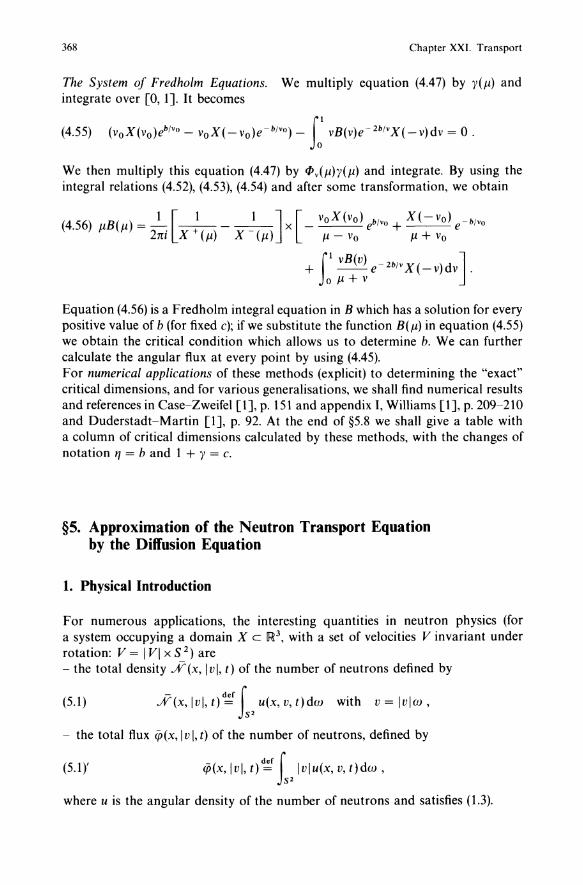
368 Chapter XXI. Transport
The System of Fredholm Equations. We multiply equation (4.47) by Y(/l) and integrate over [0, 1]. It becomes
(4.55) (voX(vo)eb/vo - voX( -vo)e- b/vO ) - f vB(v)e- 2b/vX( -v)dv = o.
We then multiply this equation (4.47) by ct>v(/l)Y(/l) and integrate. By using the integral relations (4.52), (4.53), (4.54) and after some transformation, we obtain
+ --e- 2b/V X(-v)dv. II vB(v) ]
o /l + v
Equation (4.56) is a Fredholm integral equation in B which has a solution for every positive value of b (for fixed c); if we substitute the function B(/l) in equation (4.55) we obtain the critical condition which allows us to determine b. We can further calculate the angular flux at every point by using (4.45). For numerical applications of these methods (explicit) to determining the "exact" critical dimensions, and for various generalisations, we shall find numerical results and references in Case-Zweifel [1], p. 151 and appendix I, Williams [1], p. 209-210 and Duderstadt-Martin [1], p. 92. At the end of §5.8 we shall give a table with a column of critical dimensions calculated by these methods, with the changes of notation '1 = band 1 + Y = c.
§5. Approximation of the Neutron Transport Equation by the Diffusion Equation
1. Physical Introduction
For numerous applications, the interesting quantities in neutron physics (for a system occupying a domain X c [R3, with a set of velocities V invariant under rotation: V = I VI x S 2) are - the total density .K(x, lvi, t) of the number of neutrons defined by
- der f %(x, lvi, t) = u(x, v, t)dw with v = Ivlw , S2
(5.1)
- the total flux ijJ(x, I v I, t) of the number of neutrons, defined by
(5.1)' ljj(x, lvi, t)~f Ivlu(x, v, t)dw, 8 2
where u is the angular density of the number of neutrons and satisfies (1.3).
§s. Approximation of the Neutron Transport Equation by the Diffusion Equation
We make the following assumptions:
i) the mean free path 1/.[/ (see §l, equation (1.1» is very small in comparison with the size of the domain X
ii) the point x under consideration is far from the boundary (5.2) and is far from the zones of X where the data .[, f and q
vary strongly, iii) the value of t considered is far from t = 0 (that is to say
that t is large with respect a characteristic time l/.[/.Ivl»;
we can then ShOW(211) the following result:
(5.3)
(5.4)
{if u satisfies the transport equation (1.3), (p given by (5.1)' is 'close' to a solution cp of a neutron diffusion equation, then we can write it in the form
1 ocp . f-;;j at - dlV D Vcp + .[/cp - Kcp = S ,
369
where Kcp(x, I v I, t) = r.[~(x, I v' I, I v I}cp(x, I v' I, t) I v' 12d I v' I, the "coefficients" of J IVI this equation D, .[/' .[f can be calculated starting from those of equation (1.3). Now equation (5.4) is much easier to study than equation (1.3): - firstly mathematically, diffusion equations analogous to (5.4) have been studied in Chap. XVIII, and some more simple versions have been studied in Chaps. XIV to XVIII, - more important however is that for a numerical solution on computer it is much easier to solve equation (5.4) (which we then treat in multigroup form) (see Chap. lA, §5) than equation (1.3) (which we also treat in multigroup form; see equation (1.6) of §l). We have seen this in Chap. XX where the two types of equations were solved numerically. In the majority of applications to nuclear reactors we use the transport equation (1.3) (in the multigroup form, up to m = 100 groups) to calculate the physical coefficients introduced in the diffusion equation (5.4) (in the multigroup formulation with 2 to 8 groups). In this §5, we shall give a precise mathematical meaning to (5.3) and therefore justify, from the point of view offunctional analysis(212), the validity of approximation (5.3) of "the transport equation" (1.3) by a "global" diffusion equation that is to say independent of the modulus of the velocity(213), under the essential condition (5.2)i). The difficulty in the study lies in particular in the need to compare the solutions of the transport and diffusion problems which have to be unique from the
(211) See Bussac-Reuss [I]. (212) For the point of view of stochastic processes and for the convergence of the branching process of transport to that of diffusion, we refer to Dautray [I]. (213) To study the approximation of the transport equation (\.3) by the diffusion equation (5.4) (depending on the velocities) we refer to Larsen-Keller [I] and Larsen [3].
370 Chapter XXI. Transport
conditions of these problems. Therefore in the case of evolution transport problems, if we consider the solution u of the Cauchy problem given by (1.3), satisfying the initial condition u(O) = u/ and the "absorbing" boundary conditions UIL = 0, we must determine the Cauchy diffusion problem (and therefore determine not only a diffusion equation, but also the initial and boundary conditions) in such a way that the solution ofthis evolution problem approximates the solution u in the best way possible. The study of approximation of transport by diffusion in the stationary case must cope with analogous difficulties: we must again make precise the boundary conditions for the diffusion problem as a function of those for the transport problem, and (for nonhomogeneous problems) the right hand side of the diffusion equation, in such a way as to again have:
{I) the uniqueness of the solution of the stationary transport and diffusion
problems 2) the best possible approximation of the solution u of the transport
problem by that of the diffusion problem.
To facilitate this study, we shall make the following simplifying hypotheses, both on the coefficients of the transport equation and on the given initial data and source terms, and we limit ourselves to absorbing boundary conditions for the transport equation. To study the other cases, particularly reflection boundary conditions, see Sentis [3]. The criterion chosen to compare the solutions of the transport and diffusion problems will essentially be the LaO norm to allow a point comparison between these solutions, which needs the study of transport and diffusion problems in the unusual framework L 00. We revert to the LP framework for spectral comparison of the "first eigenvalue" of the transport and diffusion operators. The comparison will be global, that is to say over the whole domain X x V and for all time t > 0, and not only under conditions (5.2)ii) and (5.2)iii); naturally this comparison will show that the approximation is more delicate near to the boundary of X and for times close to the initial time t = 0, which leads us to introduce some corrector terms called the "boundary layer" and the "initial layer". Finally this study will be carried out, as in §2 and 4, in the framework of real functions.
Remark 1. Physicists use numerous approximation methods to form the approximate equation (5.4), either directly by modelling the neutron phenomena occurring in an elementary volume dx (see Bussac-Reuss [I]), or starting from the transport equation. We give an example of this last procedure in the case where u(x, v, t) satisfies the monokinetic transport equation with homogeneous isotropic collision kernel (source q = 0), let
(E) au -at + v. Vu + l:u = cl:Ku (214)
(214) Recall: l: = Ivll:,.
§5. Approximation of the Neutron Transport Equation by the Diffusion Equation
with V E S 2, the coefficients l: and c only depend on x, and with:
Ku(x, V, t) = f u(x, v', t)dv' , S2
denoting by dv' the surface measure of S 2 divided by 4n. Set
cp(x, t) = f u(x, v, t)dv S2
J(x, t) = f vu(x, v, t)dv . S2
By integrating equation (E) with respect to v, we obtain
(5.5) 8-8~ + div J + l:cp = cl:cp .
371
The physicist replaces the unknown functions (p and J by the "approximate" unknown functions cp and J again satisfying (5.5) and makes the (approximate) hypothesis that the spatial inhomogeneity of the neutron flux cp produces the neutron current J, and also that this is characterized by
(5.6) J = -DVcp.
This law, which is used for numerous (approximate) models in physics, is called Fick's diffusion law, and D is called the diffusion coefficient. By substituting J in (5.5), we obtain the diffusion equation
(5.6), ~~ - div(D Vcp) - l:(c - l)cp = 0 .
Various approximations give various values of the coefficient D from the coefficients of equation (1.3)(215). To obtain u(x, v, t) starting from ¢(x, t), we make a truncated expansion of u in spherical harmonics(216) of v. We obtain
u(x, v, t) = cp(x, t) + 3v.J + ... + remainder.
The physicist often makes the approximation of stopping the expansion at the
linear term in V and replacing (p, J by cp, J by (5.6); therefore we have
(5.7) u ~ cp - 3Dv. Vcp .
Thus the calculation of cp produces an approximate value for u. We can verify the consistency of the approximations (5.5) to (5.7) (see Bussac-Reuss [1]). D
(215) A first approximation gives D "" lj(3};). (216) See Chap. II, §7 and Chap. VIII, §2 for spherical harmonics.
372 Chapter XXI. Transport
The object of §S.2 and S.3 below is to give the hypotheses under which approximation of transport by diffusion is valid and to establish these equations rigorously. Then in §S.4 (in the case of a stationary equation) we shall give a higher order approximation by a diffusion equation with particular boundary conditions (of Robin type) which is linked to the idea of extrapolation length. Following this in §S.S and what follows, we shall study the approximation of the principal eigenvalue of the diffusion operator - firstly with Dirichlet boundary conditions, then for higher precision with Robin boundary conditions. We shall then give an application to the approximation of the critical size associated with a transport operator. We follow the techniques of Larsen-Keller [1], Papanicolaou [1], Blankenship-Papanicolaou [1], then of Bensoussan-Lions-Papanicolaou [1] for boundary layer problems, of Sentis [2] for eigenvalue problems and of BardosSantos-Sentis [1] for problems of critical size.
2. Approximation in the Case of a Monokinetic Model of Evolution Equations and of Stationary Transport Equations
We assume that the modulus of the velocity of the particles is constant (monokinetic case). The space V of velocities is therefore S 2 equipped with the uniform
probability measure denoted dv (therefore such that IS2 dv = 1). Let X be an open set, not necessarily bounded, of [R3 whose boundary ax is regular(217). We consider the following transport problem: find the solution u = u(x, v, t) of
au - - f i) -;- (x, v, t) + v. Vu(x, v, t) + 17 dx)u(x, v, t) = 17(x) f(v', v)u(x, v', t) dv' , ut S2
(S.8) ii) u(x,v,t)=O, (x,v)ET_(218),
iii) u(x, v, 0) = u/(x, v) ,
where it and i(219) are positive bounded functions over X and where the given "collision nucleus" f is a positive function independent of x, which is measurable and bounded over S 2 X S 2 and which satisfies:
(S.9) f(v, v') =f(v',v), v, V'ES2,
(217) When we say that ax is regular we mean here that it is at least of class ~3.", 0 < at < I, (with X locally on one side of aX). (218) We recall that: r _ = {(x, V)EaX x S2; Vx.V < O} where Vx is the outward normal to ax at x. (219) We thus adopt slightly different notation in this paragraph from that of the preceding paragraphs and of Chap. I A, §5.
§5. Approximation of the Neutron Transport Equation by the Diffusion Equation 373
[this is classic in the mono kinetic case since f often only depends on (v, Vi)]; we normalise f so that
(5.10) f f(V', v)dv' = 1 . S2
Then the mean number of "secondary particles" is:
I(x) c(x) = -_-.
2'dx)
We assume that the mean free path is small compared with the dimensions of X, that is to say that II and I are large. We make the change of notation:
- 2'1 - 2' 2'1=-; 2'=-.
e e
We then change the time scale characterized by t' = te(220). We can write (5.8)i) in the form(221):
(5.11) {au 1 -a I (x, V, t') + - v. Vu(x, v, t ' )
t e
= e12 [2'(X) Is/(V" v)u(x, Vi, t') dv' - 2' I (x)u(x, v, t') ] .
Finally we make the hypothesis that c(x) is very close to 1, or more precisely that (c - 1) is infinitesimally small of order e2 , that is,
(5.12) 2' I (x) = 2'(x) - e2y(x)
where y is a bounded function. On the other hand, we make a change of notation using t instead of t'. We define the operator KO(222\ which is linear and continuous over U(S2) by
(5.13)
We firstly assume that u/ is independent of v. We first give the standard result of approximation of transport by diffusion; we shall then give many other results of the same type. (We shall use here, and in what follows, the summation convention over repeated
3
indices: "rx;/3;" denotes" L rx;{l;"). i= I
(220) This change of time scale is fundamental. It can be interpreted "physically' by saying that the time scale with which we observe the diffusion is slower than that of the physical phenomenon of transport. The diffusion is therefore happening in a macroscopic (in time) scale with respect to the transport. (221) By setting U(x, v, t') = u(x, v, t) = u(x, v, t'M and denoting U by U.
(222) Ko is called the collision operator.
374 Chapter XXI. Transport
Theorem 1. 1:, y satisfy:
Let X be an open bounded set ofIR3 with "regular" boundary, and letf,
(5.9) f(v, v') = f(v ', v), v and v' e S2 ,
(5.10) f f(v', v)dv' = 1 ; S2
(5.14) 3/30> 0, /31 > 0, /30 ~f(v, v') ~ /31
(5.15) { /30 ~ 1:(x) ~ /31 30(, 0 < 0( < 1, 1:e~3.a(X), ye~2.acX) (223)
Then there exists a symmetric matrix (aij(x)) which is positive definite with the following property:
For every "sufficiently regular"(224) function u/ = u/(x)
(u/e~4.a(x) with u/lax = 0, a~i (aij :::)L = 0) , the (strong) solution u, in ~([O, + 00 [, L':) (X X S2))(225) of the problem:
. au, 1 1 2 1) at = - ~ v. VUE - e2 1:(Ko - J)u, + yu, in X x S x ]0, + 00 [
(5.16) ii) u,(x,v,t)=O, (x,v)er_, t >0,
iii) u,(x, v, 0) = u/(x) (x, v)eX x S2 ,
the (strong) solution u in ~([O, + 00[, L,:}(X))(225) of the problem:
. au a ( au) 1) - = - aij - + yu at aXi aXj
in X x ] 0, + 00 [
(5.17) ii) u(x, t) = 0, xeax, t > 0
satisfies, for all t ~ 0:
(5.18) Ilu,(.,.,t) - u(.,t)IIL~(XXS2) ~ eeb/(1 + t)CU" where t5 = sup y(x), and where CUI is a positive constant (independent of e).
x
Ifthe open set X is unbounded, we can state a theorem analogous to Theorem 1, with conditions at infinity (essentially 1: and y must be bounded (with bounded derivatives) and we must impose lim u/(x) = 0).
Ixl-oo
(223) Recall that we denote by ~k··(X) the set offunctions u with derivatives up to order k in ~o(X), and whose derivatives of order k are Hiilderian of order Q( in X, 0 < Q( < I. (224) These conditions are not optimal and can probably be weakened. (225) We denote by L': the space L'" equipped with the weak-. topology.
§5. Approximation of the Neutron Transport Equation by the Diffusion Equation 375
In 5.5 we shall give an interpretation of this result in terms of semigroups and of convergence of operators. Before proving this theorem, we shall give a result on the operator Ko which is the basis for this proof. Denote by (., .)v duality U(S 2),
'2 . [1 1 ] U (S ), with p + P' = I .
Lemma 1. Assume (5.9), (5,10), (5.14), Let hE U(S2), P E] 1, 00,]. For a solution yin U(S 2) of the equation
(5.19) (Ko - /)y + h = 0 ,
to exist it is necessary and sufficient that
(5.20) (h, l)v = 0 .
Further, y is unique up to a given constant (in v). On the other hand, there exists a unique DiELOO(S2) (i = 1,2,3) such that
(5.21)
If we set
(5.22)
then the matrix (Xij is symmetric and positive definite, D
Proof of Lemma. The continuous operator Ko defined over U(S2), for all p E] 1, + 00 [) by:
(5.23) Kog(v) = f f(v', v)g(v')dv' S2
is a compact operator (this follows from condition (5.14) - see for example Appendix "Singular integrals", Proposition 1, §1 for pE] 1, ooD and positive in the sense:
gEU(S2) , g ~ 0 not identically zero = Kog > 0 .
Moreover the operator Ko is such that:
Kog(v) ~ 130 f g(v')dv', K~g(v) ~ 13~ f g(v')dv', S2 S2
for every universally measurable positive bounded function g (see Appendix Chap. VIII) and Ko 1 = 1. It then follows from the Doob-Krein-Rutman theorem (Theorem 3 of the appendix cited above) that 1 is a simple eigenvalue of Ko in the Banach space B(S2) of universally measurable bounded functions in S2, and therefore also in LP(S2), pE[l, + 00]. On the other hand, from the Fredholm alternative, we know that (Ko - /) is invertible in {hEU(S2),(h, l)v = O} a subspace of U(S2), pE]l, 00[: The same applies for p = + 00; indeed for all hE L OO(S 2) (and hence hE U(S2 )Vp) with (h, l)v = 0, there exists YEU(S2) such that (Ko - /)y = -h; now
376 Chapter XXI. Transport
ImKo c LOO(S2) therefore YEL CC (S2), and we can always choose y such that (y, l)v = 0; hence with the notation
the mapping h ---> Y which is the inverse of the mapping - (Ko - I) in Lo (S 2) will be continuous (from the closed graph theorem). (Note that under the additional hypothesis ''fis continuous in S2 x S2" the operator Ko will, by the Ascoli theorem, be compact from L 00 (S 2) into C(jO (S 2), and hence also into LX (S 2), and we can then apply the strong Krein-Rutman theorem in LX (S2), and the Fredholm alternative directly). Finally from the symmetry of S2, denoting by Vj the function of L2(S2) defined by v ---> Vj, we have:
(5.24) (Vj, l)v = 0 .
Hence we have the existence of D j , the unique solution of (5.21). We now define rxjj thanks to (5.22); for all ~ E 1R 3, we have, by denoting g(v) = ~jDj:
(5.25)
But, by using (5.1 0):
(Kog; g) = f f f(v, v')g(v)g(v')dvdv' S2 S2
(5.26) = -! f f f(v, v')lg(v) - g(v'W dvdv' 2 S2 S2
+ -21 f f f(v, v')(lg(vW + Ig(v'W)dvdv' , S2 S2
that is to say with (5.10) and (5.14):
(5.27) (Kog, g) - (g, g) ~ - Po [ Is2 Ig(vW dv J Therefore returning to (5.25) we obtain:
rxij~j~j ~ Po f Ig(vW dv . S2
(5.28)
We see that rxij~j~j ~ 0, and if we have for one ~:
rxij~j~j = 0 ,
this implies
g(v) = ~jDj = 0 for almost all v .
Hence by applying the operator (Ko - J), we obtain:
~jVj = 0 for almost all v ,
which is impossible. Therefore the matrix rxij is positive definite. o
§5. Approximation of the Neutron Transport Equation by the Diffusion Equation
Proof of Theorem 1 1st stage. (Formal) Expansion. We write u, in the following form:
u, = Uo + WI + C2U2 + 1/1,(226) .
We replace u, by this expansion in (5.16)i) and we look for UI such that:
(5.29)
(5.30)
(Ko - 1)uo = 0
l:(Ko -1)UI - v. Vuo = 0
OUo (5.31) l:(Ko - 1)U2 - v. VUI - -:1- + yuo = 0 .
ot To satisfy (5.29), then (5.30), we take:
(5.32)
377
From the preceding lemma it is necessary and sufficient for there to exist a U2 satisfying (5.31)i) that:
( OUI auo ) 1, - Vi - - - + yuo = 0 OXi at v
which can be written:
OUo ( a D j ouo) -= 1 v·----- +yuo at ' I aXi l:(x) OXj v
a rJ.ij oUo = - -- -- + yuo .
OXi l:(x) aXj
We therefore obtain the first line of (5.17) provided we set: rJ. ..
(5.33) aij(x) = l:(/~) .
Take Uo = U the solution of (5.17). Take UI given by (5.32) and U2 the solution of (5.31) with (U2' l)v = O. Write the equation satisfied by 1/1, obtained by replacing u, by its expansion and taking account of (5.29), (5.30), (5.31):
01/1, 1 1 --;- = -- V VI/I, + zl:(Ko - 1)1/1, + yl/l, + cgl ut C C
(5.34) 1/I,(X,v,t)=Cg2(X,V,t) , (X,V)Er_, t>O,
I/I,(X,V,O) = Cg3(X, v) , (X,V)EXXS 2 ,
(226) Note that it is necessary to include terms of second order in e in this expansion to obtain a comparison (5.18) to first order in e because of the terms in second order in e in equation (5.16)i).
378
with
(5.34)'
aUI [auz ] gl = -v. Vuz - at + YUI + B -at + yuz
DiaUo + gz = - - ~ - BUz on T _ x IR ,
1: aXi
Chapter XXI. Transport
g3(X,V) = -udx,V,O)-BUz(X,V,O), (X,V)EXXS Z
2nd stage. We note that the operator (1'. - M) defined in LI(X x V) by:
{
1 1 (1'. - M)w = - - v. Vw + 2: l:(Ko - J)w + (y - b)w, IfWED(1'.)
B B
D(1'.) = {WEWI(XX V), wlr_ =O}
is dissipative in L I (X x V), and is therefore the infinitesimal generator of a contraction semi-group (G'(t)e-.lI)I>o (of class ct'0) in LI(X x V) where (G'(t))Po is the semi group generated by the transport operator 1'.. Likewise by duality in L 00 (X x V), (G'(t)e - .l1)1> ° is a contraction semigroup (but not of class ct'0), hence
IIG'(t)II2'(c(xXV)) ~ e.ll , 1ft> O.
Since (G'(t))I>O is also a positive semigroup (in LOO(Xx V)), we deduce that if e-.llgl(.,t) and e-.llgz(.,t) are essentially bounded over Xx VxJO, +oo[ and T _ x JO, 00[, the solution '1', of (5.34) satisfies:
(5.35) Ilt/I,(.,t)lloo ~ Be.llllg31100 + e f~ e.l(I-S)(llgd·,s)lloo + Iblllgz(·,s)lloo)ds
~ BCoe.ll (1 + t) ,
where we have denoted the norm in L 00 (X x V) and in L 00 (T _) by II 1100' and where Co is a positive constant (only depending on ud. It then remains to verify that
e-.llgdt)ELOO(Xx Vx(O, + (0)) and e-.llgz(t)ELOO(T_ x (0, +(0))
and that IluI(.,t)lloo ~ Cle.ll , Iluz(.,t)lloo ~ Cze.ll .
This can be done under regularity hypotheses on the initial data Uf.
3rd stage. We assume that the open set X is bounded. In the Banach space ct'o(X) = {UEct'(X), uliJX = O}, the diffusion operator A(ZZ7) defined in ct'o(X) by:
lAU = aa aij :U + yu, IfUED(A), (5.36) Xi Xj
D(A) = {UE WZ,P(X), Ifp > 3, uliJX = 0, Au Ect'(X), AuliJX = O}
(227) Not to be confused with the convection operator, also denoted by A in the preceding paragraphs.
§5. Approximation of the Neutron Transport Equation by the Diffusion Equation 379
is the infinitesimal generator of a holomorphic semigroup in C(f o(X), denoted by (G(t»t>o, with IIG(t)11 ~ edt, (A - M being dissipative in LI(X»; see Pazy [1], p. 217. (Note that by the regularity theorems-see for example Gilbarg-Trudinger [1], p. 101 and 106-we have D(Aoo) = n D(A") C C(f4.a(X».
" The control of the functions Ul, U2, g2, g3 in the L 00 norm can be carried out without great difficulty by:
II auo II dt lIud·,t)lIoo ~ Co sup aXj (.,t) 00 ~ C1e ,
IIU2(·,t)lIoo ~ Co max (s~; lIa~:~:j (·,t)t, s~p 1I::j (·,t)t) ~ Cledt ,
(denoting various constants by Co, C I, C), therefore
IIg2(.,t)1I00 ~ Cedt .
The control of g 1 in the L 00 norm is more difficult; it involves
auo i) through v. VU2 the terms (v. V)3 UO v. Vat '
. aUl auo 1) through at' the term (v. V) at '
. aU2 a2uo 2 auo 1) through at' the terms at 2 and (v. V) at .
We can verify with the help of interpolation results (see Bergh-Lofstrom [1]) that under the indicated (regularity) conditions on u/ and the coefficients Land y, we obtain:
IIgI(.,t)lIoo ~ Cedt ,
from which we finally deduce with (5.35):
{ "U,(.,t) - u(.,t)lIoo ~ II 1/1,(., t) 1100 + ellud.,t)lIoo + e2I1u2(.,t)lIoo ~ eCedt(l + t) ,
and hence we have Theorem 1. D
Before giving some examples, we shall state the result, analogous to the preceding one, for the stationary transport equation. From the results of §2, we know that if y(x) ~ Yo < 0, then equation (5.38) in the theorem below has a unique solution in Loo(XXS2).
Theorem 2. We make the same hypotheses as in Theorem 1 (but here the regularities LEC(f2,a(x) and YEC(fI.a(X) are enough) and moreover we assume that
(5.37) y(X) ~ Yo < 0 .
Let g be given (independent of v) and satisfying(228):
(5.37)'
(228) In the case where X is unbounded, a further condition is imposed at infinity, for example lim g(x) = O.
Ixl ..... oo
380 Chapter XXI. Transport
Then the matrix (aij(x)) chosen in Theorem 1 allows us also to have the following property: the unique solution u, in L 00 (X x V) of the stationary transport problem:
1-! v. VUE + 12 L(Ko -l)u, + yu, + 9 = 0 ,
e e
u,(X,V)=O, (x,v)EL,
in X x S2 ,
(S.38)
and the unique solution u in L 00 (X) of the stationary diffusion problem:
(S.39)
satisfy:
(S.40)
1. a ( au) 1) - aij - + yu + 9 = 0, in X
aXj aXj
ii) ulax = 0 .
with Cg a positive constant (depending on 9 and not on e).
Proof The principle of the proof is identical to that of Theorem 1. We set
u, = Uo + WI + e2U2 + "', and Uo and UI must satisfy equations (S.29) and (S.30) and (S.31) is replaced by
(S.41) L(Ko -l)U2 - V. VUI + YUo + 9 = O.
The existence condition for U2 then gives (S.39)i). The regularity theorems for Holderian functions (see Gilbarg-Trudinger [1]), give Uo E ce3 • ~(X) for 9 E ce I. ~(X) with the required regularity results on Land g, and consequently U2Ecel·~(X), V. VU2 E ceo. ~(X). Theorem 2 then follows. D
Example 1. The case of an isotropic collision operator K o. We assume thatf= 1, then we have:
(S.42) Dj(v) = Vj , 1
!Y.jj = "3 Jij (Jij the Kronecker symbol)
and (S.17)i) is written:
au d' ( 1 ) at = IV 3L Vu + yu ,
which is equation (S.6)' with D = 1/(3L).
Example 2. The case of the infinite band and the isotropic collision operator. We consider an infinite band in [R2 or [R3, with thickness a (on the transversal axis (x)) and invariant under translations orthogonal to the axis (x). If 11 denotes the cosine of the angle which the velocity makes with the direction (x) then instead of problem (S.16) we can model the transport process by the following
§5. Approximation of the Neutron Transport Equation by the Diffusion Equation 381
[ f +l d 'J problem assuming thatf=:: 1, therefore Kog(/l) = -I g(/l'); :
(5.43)
-;-= ---;-+2L(X)(Kou,-u,)+,),(x)u" XE[O,a], /lE[-l, + 1 , ut c uX c {au, /l au, 1 ]
u,(O,/l,t)=O, (/l >0); u,(a,/l,t)=O, (/l< 0),
u,(x, /l, 0) = u/(X) ;
then the result of Theorem 1 remains true with (5.17) replaced by
{
~~ = :X G :~ ) + ')'u ,
(5.44) u(O, t) = u(a, t) = 0 ,
u(x,O) = u/(x) .
We have an analogous result for the stationary case.
Example 3. Now suppose that, besides the hypotheses of Theorem l,fis invariant under the action of the group O(S2) oflinear transformations leaving the sphere S2 invariant (i.e. rotations and symmetries(229) that is to say:
(5.45) f(Rv, Rv') = f(v, Vi), V R E O(S2) ;
this is the case, for example, when f only depends on the scalar product v. Vi. We shall show that in this case there exists a constant eo > 0 such that
(5.46) (Xij = eol5ij [l5ij the Kronecker symbol] .
We shall use this result later.
Proof of(5.46). For every transformation R E O(S2), we denote by fYi the continuous operator in L2(S2) (or more generally U(S2) with pE[I, + 00], but it is sufficient to take p = 2) defined by:
fYiu(v)=u(R-1v), VES2.
We firstly verify by using (5.45) that
fYiKou(v) = Kou(R - 1 v) = f f(R - 1 v, v')u(v')dv' S2
therefore,
(5.47) fYiKo = Kogp .
(229) Note that it is sufficient to have the invariance off by rotation to have (5.46).
382 Chapter XXI. Transport
Moreover the space LMS2) defined by:
L~(S2) = {uEL2(S2), (u, l)v = O}
is invariant by 0(S2). We denote by uf the solution in L~(S2) of the equation (J - Ko)u = /; therefore Di = UVi . From (5.47), we have
therefore
(5.48)
and therefore
(5.49)
and for g(v) = ~iDi(V) = U~iVi(V) = u<~·v>(v) = U~(V)(230)
9lg(v) = g(R-1v) = u.>t~(v) = (R~)iDi(V);
therefore, with (5.25) we obtain
(5.50) { C(ij(R~);(R~)j: =- (Ko91g, 9lg)v + (91~ 9P.g)v . - (Kog, g)v + (g, g)v C('J~'~J'
Thus the quadratic form C(ij~i~j is invariant under rotation, which implies the existence of a constant eo such that
C(ij~i~j = eo I. a, \f~E 1R3 , i
from which we have (5.46). D
Remark 2. We make the same assumptions as in Example 1 with/= 1. Integrating (5.l6)i) with respect to v and setting (as in the introduction)
CfJE(X, t) = r uE(x, v, t )dv , JS2
JE. i = r ViUE(X, v, t )dv , JS2 (JE is called the current of particles), we obtain:
OCfJE 1. ----;- = - - dlV J, + YCfJ, . ut E
Under the conditions of Theorem 1, we have:
CfJ,(x, t) --+ u(x, t) as E --+ 0 ,
(230) By identifying ~ = (0 with the linear form VE ~3 ---> <~, v) = ~iViE~, so that R~ is identified with 91~.
§S. Approximation of the Neutron Transport Equation by the Diffusion Equation 383
where U is the solution of (5.l7). Moreover, relation (5.32) implies (by (5.42)):
Therefore we have:
(5.51) 1
J, = - e - Vu + 0(e 2 ) . 31:0
In this sense the procedure above allows us to estimate the approximation which constitutes relation (5.6). 0
3. Generalisation of Section 2
3.1. Case where the Given Initial Condition UI Depends on v
We begin by generalising the hypotheses made on the initial condition:
Theorem 1'. Under the hypotheses of Theorem 1, but with the initial condition Ul depending on VES2, such that, with iil(x) = (Ul(X,,), l)v:
(5.52) { ~~U/~:oo~XXS~) (231), _ O:s.; letl:s.; 3, UlEct' ' (X), ullax = AUllox = 0 ,
the (strong) solution u, of (5.l6) and the (strong) solution U of problem:
(5.53) 1. au a au 1) at = - aij - + yu in X, t > 0
ii) u(x, t~: 0 ,OX~EOX' t > 0
iii) u(x, 0) = (Ul(X,,), 1)v = iidx), x EX,
satisfy the following property: there exists a function w = w(x, v, 8) (depending linearly on Ul) such that 8-+ w(.,., 8)Ect'([0, + 00 [,Loo(X X S2)) and:
{i) Ilw(.,8)1100 -+ 0 as 8-+ + 00, in Loo(X x S2)(232)
(5.54) .. 2 nt + 11) II u,(.,., t) - U(., t) - w(.,., tie) II 00 :s.; ee (1 + t )CUI' Itt E IR .
with a positive constant CUI independent of e.
We give the proof of this Theorem l' in the appendix.
(231) D~UI denotes the partial derivatives at x of order C( of UI'
(232) More precisely, there exists a constant C( > 0 such that II w(.,., 0) II ~ e- 08 11 UI II ~.
384 Chapter XXI. Transport
3.2. The Non-monokinetic Case. Global Approximation
We now consider a more general case than in §5.2. Let X be an open subset of [R".
The sphere S2 is replaced by a subset V of [R" satisfying
(5.55) 1 V is a compact union of spheres centred at 0 equipped
with a probability measure which is invariant under every
rotation (or symmetry) R with centre 0 (REO(S"-l».
For example V could be a shell
V = {VE [R3, VI ~ Ivl ~ vs}
equipped with a uniform probability, or V could be the union of a finite number of spheres centred at 0, and the restriction of the measure defined over V to each of these spheres is uniform (this corresponds to the "multigroup" model). Withf a positive function over Vx V satisfying (5.14), we define the operators Ko and Ko by:
(5.56) Kog(v) = Iv f(v', v)g(v')dv', Kog(v) = Iv f(v, v')g(v')dv' .
We also denote by ( .,. )y the duality U' (V), U' (V), P E [1, + 00]. We shall make hypothesis (5.45) but not hypothesis (5.9) (indeed, in applications, in the multigroup case the probability of going from an energy level "1" to an energy level "2" is different from that of going from "2" to "I"). On the other hand, we make hypothesis (5.10). Therefore the operators Ko and Ko are compact in U(V), p E] 1, + 00 L (see Sect. 2), are positive (in the sense that <P ~ 0, <P not identically zero=Ko<p>O and Ko<p>O) with Kol=l; as in Sect. 2, by the Doob-Krein-Rutman Theorem, we deduce that 1 is a simple eigenvalue of Ko (with p(Ko) = 1) and this is therefore also true for its transpose Ko, (relative to all the spaces U(V),pE[I, + 00]). Hence:
(5.57) 3nELOO(V) which is unique, Kon = n, n ~ 0, (n, l)v = 1.
By (5.45) and (5.57), we have n(Rv) = n(v) and from symmetry, we have:
(5.58) (n, Vj)v = 0 .
We can then state the following lemma, based, like Lemma 1, on the Fredholm alternative.
Lemma 2. Let Ko be defined by (5.56) and n satisfy (5.57) and (5.58). For there to exist a solution y E U( V), P E ] 1, + 00 ] of the equation:
(5.59) (Ko - I)y + h = 0, for given h, hEU(V),
it is necessary and sufficient that (h, n)v = O. Further the solution of(5.59) is unique up to a constant. On the other hand, there exists a unique DjE L OO(V), such that: (Ko - I)D j + Vj = 0, (n, Dj)v = 0 and the matrix defined by a.ij = (n, vjDj)v is positive definite.
§5. Approximation of the Neutron Transport Equation by the Diffusion Equation 385
Since we have made hypothesis (5.45), we show in the same way as in Example 3 that there exists a constant eo such that:
By Lemma 2, the operator (Ko - I) is therefore invertible as a mapping of L:' (V) = {u E L OO(V), (u, n)v = O} into itself (with continuous inverse). We now state the analogue of Theorem l' (with an initial condition which is a function of x and v).
Theorem 3. Let X be an open bounded set(233) of [Jtn with regular boundary. Let V be a compact union of spheres centred at 0 equipped with a probability measure which is invariant for all R E o(sn-1) and let f, I and y satisfy:
(5.10) Iv f(v', v)dv' = 1 ,
(5.14) 3/30, /31 E IR+; 0 < /30 ~f(v, v') ~ /31; /30 ~ I(x) ~ /31 , (5.15) IE CC 3. a(x); y E CC2. a(x) ,
(5.45) f(Rv, Rv') = f(v, v'), VR E o(sn - 1) .
Then there exists a positive definite symmetric matrix (aij(x)):
(5.60) eo
aij(x) = I(x) bij (eo constant) ,
having the following property. Let UI be the initial data satisfying (with UI(X) = (UI(X,.), n)y):
(5.61)
D~UIELOO(XxV), 0~1(X1<3, U1ECC4 • a(X), ullax=-aa aijaaU1 I =0; Xi Xj ax
let u, be the (strong) solution in CC( [0, + 00 [, L';; (X x V)) of:
t B e 1 aaU' = -! v. VUE + 12 I(Ko - l)u, + yu" (x, V)E X X V ,
(5.62) u,(.,t)IL = 0 ,
u,(x, v, 0) = UI(X, v) ;
and u the (strong) solution in CCo([O, + 00 [, L';;(X)) of:
1 au = ~ (aij ~) + yu, X E X at aXi aXj u(.,t)lax = 0 ,
u(.,O) = (UI("')' n)y
(5.63)
(233) If the open set X is unbounded, this theorem remains true under the hypotheses indicated in Theorem I; we must therefore also have, besides (5.61), lim u,(x, v) = O.
Ixl-OC!
386 Chapter XXI. Transport
then there exists w = w(x, v, (}) such that ()-> w(. ,.,O)Ec€([R+, L"'(X x V» and:
(5.64) {IIW(.,O)IILJ(XXV)->O as 0-> too, at Ilu,(.,.,t)-u(.,t)-w(.,.,t/c )IIL'(xxv)~CCe (1 +t), \/t>O.
The analogue of Theorem 2 is stated in the following way:
Theorem 4. Under the same hypotheses as in Theorem 3 (with only l: E C€2. a(x), YEC€l.a(X» and assuming also
(5.65) y(x) ~ Yo < 0 ,
Let u, be the unique solution in L 00 (X x V) of:
(5.66) l-! v. VUE + ~ l:(Ko - l)u, + yu, + g = 0 , £ £
u,(x,v)=O, (X,V)Er_
in X x V ,
where the given data g only depends on x and satisfies
(5.67)
Since the matrix aij is the same as in Theorem 3, given by (5.60), if u is the unique solution in L 00 (X) of:
I a~j (aij ::J + yu + g = 0, in X , (5.68)
ul,lx = 0 ,
then we have:
(5.69) II u, - u II c(X x V) ~ cCg , Cg a positive constant.
3.3. LP Estimates
We can also obtain, in the framework of Theorem 3 (for u/ in L 2(X x V), with X bounded or otherwise) some error bounds in the L2(X x V) norm and therefore in the U(X x V) norm (for 2 ~ p < + 00 ).
3.4. The Case where f Depends (Regularly) on x
In the framework of Theorem 3, we can also assume that! depends regularly on x; then the functions 1t and Dj depend regularly on x; we must replace the first line of (5.63) by
(5.70) au a ( au) au -;- = -;- aij -;- + bj -;- + yu , ut UXj uXj UXj
(234) With, if X is unbounded, a condition at infinity such that lim g(x) = O. Ixl-oc,
§5. Approximation of the Neutron Transport Equation by the Diffusion Equation 387
with
3.5. Perturbation of the Operator T. by a Bounded Integral Operator
Again in the framework of Theorem 3, we can consider u, the solution of:
(5.71) lou, 1 L --;- = - - v. VUe + z(Ko -l)u, + YU, + Hu, , ut 8 8
u,(.,.,t)lr_=O, u,( . , . ,0) = u/ ,
where H is the following operator:
Hg(x, v) = Iv (/(x, v, v')g(x, v')dv' with (/ELOO(X x Vx V);
then Theorem 3 is again true (see Sentis [1], Chap. 3) if we replace the first line of (5.63) by:
(5.72) ~~ = O~i (aij ::j) + (y + (HI, n)v)u .
This formulation will be more useful in practice when we know that the total cross-section (L + 8 2 y) and the differential cross section (L f + 82(/) have little variation from a mean value with x in some subdomain X' of X (then LO is constant on X').
3.6. Another Generalisation
We can finally consider some more difficult problems in which the operator L(Ko - 1) is replaced in (5.62) by the following operator, L, with domain dense in L 2(Z x V)(235) (where Z is the torus lf3 with If identical to the interval [0, 1] where we have identified 0 and 1) given by:
Lg(z, v) = - Vi ~g (z, v) + r (/J(z, v, v')g(z, v')dv' - (/(z, v)g(z, v) uZi Jv
with the condition of having hypotheses which allow us to confirm that 0 is a simple eigenvalue of L and that we have:
(Vi, n)L2(Zx V) = 0 where n is nonzero and satisfies: (Lg, n)e(zx V) = 0 ,
VgED(L) .
For this, see Bensoussan-Lions-Papanicolaou [1] and Sentis [1].
(235) Or more generally in LP(Z x V), pE] I, 00 [, with analogous hypotheses on 0"1 and 0" to those made previously on f and E.
388 Chapter XXI. Transport
3.7. Adjoint "Type" Problem
Instead of (5.62), we can obviously consider the problem:
l °"'U'=~v.vu,+ lzL(Ko -l)u,+yU" (X,V)EXXV, t>O, ut 8 8
(5.73) u,(.,.,t)lr+ =0,
u,( . , . ,0) = u/ .
Under the same hypotheses as in Theorem 3, with u the solution of (5.63), we also obtain (5.64); only the function w will be different [indeed, by the symmetry properties offwe have, with D;-(v) = D;( - v):
((Ko -l)D;)( - v) = v; = (Ko -l)D;-(v) from which D;- (v) = - D;(v) .
therefore:
(5.74) (n, - Vie - D;))v = lXij] .
Note that if we replace Ko by K~ in (5.73) we obtain the adjoint problem of (5.62). The generalisation above, as before, can be extended to the stationary case without difficulty.
4. Calculation of a Corrector for the Stationary Problem and Extrapolation Length
In this Sect. 4, we shall make the same assumptions as in Theorem 4 and we shall look for an approximation of order 8 z ofthe solution u, of (5.65). We shall see that if we introduce a diffusion problem with a particular boundary condition (of Robin type), which corresponds to the concept of extrapolation length used in neutron physics (see Introduction), then we can obtain a second order approximation of I u,(x, v)dv.
Proposition 1. Make the hypotheses(236) of Theorem 4 with g E ~2,a(x), X bounded(237). Let u, be the solution of(5.66). Let u and w be the solutions ofthefollowing problems:
(5.75) {i) - ~ (aij~) - yu = 9 ,
OX; OXj
ii) uliJX = 0 ,
in X ,
(236) But we must assume a little more regularity on ax and the coefficients Land y: for example ax of class qr4," with L E qr3,"(X) and y E qr2,"(X) and to justify the expansions made in what follows, we must take a priori g E qr2,"(X), which will give U E qr4,"(X), (see Gilbarg-Trudinger [IJ, p, 105) and
- E qr3·"(aX), aul _ an iJX
(237) To simplify the statement.
§5, Approximation of the Neutron Transport Equation by the Diffusion Equation 389
{i) - ~ (aij ow) - yw = 0, in X ,
ox; aXj (5,76)
)')') L au wi ilX = - 1: av '
where L is a positive constant (independent of the given data g); then for every space U(1 ~ P < (0):
Il u, - [u + £(- Di~aau + w)JII ~ £2Cp ,g 1: Xi LP(XxV)
(where Cp,g is a constant and Di is defined as in Lemma 2),
Proof In the same way that we made an expansion of u, up to second order in £ to have an 0(£) approximation to the solution we shall make an expansion of u, up to third order to have an 0(£2) approximation:
u, = u + WI + £zuz + £3 U3 + t/I, . By substituting this expansion of u, into equation (5.66), we see that we must choose u, Ul, Uz, U3 satisfying:
(5.77)
(5.78)
(5.79)
(5.80)
(Ko - /)u = 0
au 1:(Ko - J)UI - Vi~ = 0
aXi
aU I 1:(Ko - J)uz - Vi - + yu + g = 0
aXi
auz 1:(Ko - J)U3 - Vi-a + YUI = O.
Xi
From Lemma 2, equations (5.77) and (5.78) give:
(5.81)
(5.82)
u = U(X) (Z38)
Di au UI = - - ~ + w where w = w(x) ,
1: aXi
and for (5.79) to have a solution U2 it is necessary and sufficient that:
a 1 au ~a ~(1t,viDj)y-a +yu+g=O
Xi"- Xj
that is to say, (5.75)i). For u take the solution of (5.75). Equation (5.79) is then equivalent to:
(238) When we write u = u(x) this means that u depends only on x and not on v,
390 Chapter XXI. Transport
Therefore denoting by h a solution of:
(5.83) o [1 OUJ (Ko - l)h = - OXj 1: (Vj Dj - aij) OXj ,
we obtain.
(5.84)
Equation (5.80) is then rewritten in the form:
E(Ko -I)U3 - Vj ~ (~) + Vj ~ (Dj ) ow _ y Dj ~ + yw = 0 . OXj E OXj E OXj E OXj
For this equation to have a solution, it is necessary and sufficient that:
(5.85) ~ aij ow + yw - ~ (n, vjh)v ~) = 0 . OXj OXj OXj E
But as the right-hand side of (5.83) is an even function(239) of v, we see that h is an even function of v and therefore we have:
(5.86)
(in fact n is also an even function). Therefore (5.85) can be written in the form (5.76)i). With the preceding choice of functions U,UbU2,U3, we obtain that r/I, must be the solution of the problem:
with
( D. Vu )1 gt = - V. VU3 + YU2, g2 = - utliJX = -E- - w iJX' g3 = - (U2 + 6U3)liJX •
Since D depends a priori on v, it is not possible to choose wliJX so that Y2 = 0 on r _, and thus it does not allow r/I, I r _ to be a second-order term in 6 2.
Despite this, it will be possible to choose data on the boundary for w so that the preceding expansion, written:
u, = U + BUt + 62 U2 + 63U3 + r/I, , leads to an inequality of second order in 6 2 from Proposition 1 for the LP norm, p E [1, + 00[; this is what we shall now prove with the help of an additional (to ud term, called a boundary layer term which has an U bound in 6 (of order 6). Since oX
(239) Recall that by (5.45), f is invariant by symmetry v -+ - v.
§5. Approximation of the Neutron Transport Equation by the Diffusion Equation
is regular, there exists a constant b > 0 such that the variables
x E ax, y = (x - x). n(x) (240)
391
form a system of coordinates for the layer {x E X; d(x, aX) ~ b}. For fixed x, set:
(5.87) y x-x
I] = - = --.n(x). e e
( X - x ) To add a corrector term to u" denoted b, -e-, _. n(x), v ,bx = bAI], v) must
satisfy
(5.88) {
A abx + - v. n(x) ary - L(Ko - I)bx = 0, I] E IR , V E V
Di auo A A A
bAO, v) = --a (x) - w(x) , v.n(x) < 0 . L Xi
This problem is the Milne problem in a half-space with the value of the solution given on the boundary; this problem is classical and difficult; in the appendix of §3 we show the following result (where V _ = {v E V; v. n(x) <).
Lemma 3. For every </J E L 00 (V _), there exists a unique solution U = Ux E L 00
(IR+ x V) of the problem
(5.89) {au
- v.n(x)ary -L(Ko - I)U = 0 ,
U(O,v) = cp(v) , VE V_ ,
and there exists a constant G(</J) such that if 1]-> + 00, we have:
U(I], v) -> G(cp) .
The mapping </J -> G( </J) is linear and continuous over L 00 (V _ ) and satisfies:
G(1) = 1; G(</J) ~ 0 if </J > 0 .
Let us denote now, for each x in ax (with the notation n = n(x)):
v = - v.ln + vII where V.l = - v.n(x) (therefore v. V= - V.l :n + vII. V) and denote by DH(V) the solution of:
(5.90) (Ko - I)DH + V.l = 0, Iv n(v)DH(v)dv = 0 ,
and Dxll(v) the (n - l)tuple of functions which are solutions of:
(Ko - I)Dxl1 + vII = 0, Iv n(v)Dxl;(v)dv = 0 .
(240) nix) denotes the outward normal to ax at x.
392 Chapter XXI. Transport
We obtain DX/l(v) = - Dx/l(2(v. v)v - v). From this property we can deduce, by the same techniques as in Lemma 3, that:
(5.91) G(Dx;;)=O, VXEaX.
Therefore the solution bx of (5.88) can thus satisfy
1 au 1 lim bAI}, v) = - w(x) - G(Dx.d - -a + G(Dx;;) ~ Vxu ~~CX) l: n k
1 au = - w(x) - G(Dx.d--a (x), "Ix EaX.
l: n
We therefore impose on w the following boundary condition
(5.92) w(x) = - G(Dx.d ~ aau (x), "Ix E ax . l: n
(We see that (5.85) with boundary condition (5.92) has a unique solution w). This boundary condition implies:
(5.93) lim bAI}, v) = 0, "Ix E ax ~~CX)
(that is to say that bx is a boundary layer term. On the other hand we show in the appendix of §3, that in the case where n = - en, we have:
(5.94) G(Dn) = L a positive constant.
Therefore:
(5.95)
and (5.92) can be written in the form (5.76)ii). To finish the proof, it is sufficient to set:
[ ( Di au ) z z (x - x • )] (5.96) s, = u, - u + I:: -1:" aXi + w + I:: Uz + I:: U3 + I::bx -1::- n(x), v
and to show that (for 1 ~ p < CJJ) we have:
(5.97)
Now s, satisfies:
- - Vi -a + 2: l:(Ko - l)s, + ys, = I:: 8, I:: x· I:: {las, 1 z
s,(x, v) = ~z (i(x, v), (x, v) E L ,
in which (i is a bounded function over Land 8, is a bounded function over (X' x V) for every compact set X' included in X. Hence we have (5.97) and,
(241) This inequality is also satisfied for p = + OCJ so that s, is a second order approximation to u, in the L", norm.
§5. Approximation of the Neutron Transport Equation by the Diffusion Equation
consequently, the inequality of Proposition I by noticing that:
Ix x v I bx ( x ~ x. n(x), v) IP dx dv ~ Cpt: .
Now set
(5.98) u,(x) = u(x) + t:w(x) ,
u being the solution of (5.75) and w the solution of (5.76).
Corollary 1. The function u, satisfies (under the hypotheses of Proposition I):
{
a ( au,) _ - - a·· - - yu = g X E X OXi I} OXj " ,
_ Lou, 2 Law u + t: - - = t: - - X E ax
, }: an }: an '
(5.99)
and further
(5.1 00)
where n(v) is defined by (5.57).
Since L is positive, we can easily show that the equation:
(5.101)
_ ~ (a .. OV) _ yV = g OXi I} OXj • ,
LoV V + t: - - = 0, X E ax ,
}: an
XEX
393
o
o
has a unique solution in !6'2.a(X)(242) and if g ~ 0 then V ~ O. We set the following definition:
Definition 1. For a second-order equation of type (5.101)i), a condition of the type oV
V + I a;; = 0 with I > 0 is called a Robin boundary condition.
We see that t:LI}: is interpreted as an extrapolation length(243) (that is the distance between ax and the curve where V is zero if we extrapolate linearly from the boundary oX).
Theorem 5. Let X he an open bounded(244) set of [Rn with regular boundary and V a compact union of spheres in [Rn with centre at O. Let f, }: and y be such that:
(5.10) Lf(V" v)dv' = 1
(242) For the regularity of U starting from that of g. see for example Gilbarg-Trudinger [1]. p. 122 (if 9 E '6"(X), U E '62 ·"(X». (243) Recall that f. and L are dimensionless and that 1/.[ has the dimension of a length. (244) To simplify the statement.
394 Chapter XXI. Transport
(5.14)
(5.15)
(5.45)
(5.65)
3/30, /31 E ~+, 0 < /30 ~f(v, v') ~ /31 ;
/30 ~ 1'(X) ~ /31 with l' and I' regular (245)
f(Rv, Rv') = f(v, V'), VR E o(sn-l) ,
with y(x) ~ Yo < 0 .
Let aij be the matrix (eo constant defined in (5.46))
Let Ue be the solution of
(5.102) { -! v. VUe + 12 l'(Ko - l)u, + YUe + g = 0, (X, v) E X X V
e e
uelr _ = 0 ,
where g only depends on x and satisfies g E ~2.a(X); and let V be the solution of
{ a~i (aij ~~) + yV + g = 0 ,
(5.101) L av V + e - -a = 0, on ax .
l' n
Then for all p(l ~ p ~ 00)
In X,
(5.103) II r ue(·, v)n(v)dv - vii ~ e2 Cp•g . Jv LP(~ This result is a consequence of the corollary stated above and of the (easily verifiable) fact that Ilae - VIILP(x) ~ e2 Cp•g .
5. Convergence of the Principal Eigenvalue of the Transport Operator
We now make the same hypotheses as in Theorem 3, that is, that!, l' and y satisfy (5.10), (5.14), (5.15), (5.45), and we further assume (for simplicity) that X is an open bounded, convex, regular subset of ~n. We denote by Te the operator:
(5.104)
(245) That is to say, with the regularities stated in Proposition I (for example L E <ti3 ··(X), Y E <ti2 ··(X)).
10.4 Spherical Coordinates, Spherical Harmonics, and Bessel Functions 395
Now
1(1 + 1) dv= ---v and r2
R /'(/' + 1) +1 2rr
(v,dw) = J drr2 2 J dcos8 J dcpYt". Yl'm' o r - 1 0
= R/,(/, + l)<Ylm , Yl'm')
= (dv,w) = Rl{l+ l)<Ylm ,Yl'm')'
so that <Ylm" Yl'm') = 0 for I i= /', In particular, since PI - Y/O,
+1
J dxPb)Pdx) = 0 for I i= l' , -I
10.4.3 The Radial Equation, Bessel Functions
Finally, we need to consider the equation (10.4.6):
- - rF(r) + P - -- F(r) = 0 . 1 d2 (1(1 + 1)) r dr2 r2
With F (r) = rnf(r), since
1 _(rn+1 f)" = rn f" + 2(n + l)rn- 1 l' + n(n + l)rn- 2 f r
we obtain the equation
For n = - 1/2, if we set x = kr and f(kr) = u(x) so that
we find:
1/ 1 I (1 V2) 0 u +-u+ -- u= X x 2
(10.4.33)
(10.4.34)
(10.4.35)
(10.4.36)
(10.4.37)
(10.4.38)
(10.4.39)

396 Chapter XXI. Transport
Before proving the convergence of WE to w, the first stage is to prove a lower bound
for WE' (We obviously have WE ~ sup y(x) = 15). Now this can be done only by virtue of the characterisation of WE as the type of the semigroup (GE(t)).
Proposition 2. Under the hypotheses of Theorem 3 and,further, with X bounded and regular we have, as e -+ 0:
(5.111) lim inf WE ~ W (249) . E~O
For the proof we refer to Sentis [2]; let us mention only that it uses (5.108) with the function g such that
(5.112) {
0 ~ g(x) ~ 1 ,
g(x) = 0 , if x ¢:Xo,
g(x) = 1, if x EX.
where X 0 and X 1 are two open sets such that
(5.113)
and that we have, as t tends to infinity:
(5.114) e- W1 G(t)g -+ [f g(x)cp(x)dx ] cp in L2(X) , Vg E L2(X)
where cP is the eigenfunction of the operator A characterised by:
(5.115)
We can show that the eigenvalue WE of TE is simple (see §3) and therefore we can give
Definition 2. We denote as the principal eigerifunction of the operator T. the function cPE of D( Tt ) satisfying
(5.116)
Likewise we denote as the principal eigenvalue of A the real value w, and as the principal eigenfunction the function cP of L 2(X) satisfying (5.115).
We then have:
Theorem 6. Let X be an open, bounded, regular, convex subset of ~n. Under the hypotheses of Theorem 3, WE being the principal eigenvalue of TE and W the principal eigenvalue of A, we have:
(5.117) WE -+ W as e -+ 0 .
The principal eigenfunction CPE of Tt satisfies
(5.118)
where cP is the principal eigenvalue of A.
(249) Note that this result implies that the family lV, is bounded.
§5. Approximation of the Neutron Transport Equation by the Diffusion Equation 397
Outline of Proof We denote by <. , .) the scalar product in L 2 (X x V ). We use the following lemma (see appendix of §5 and Golse-Perthame-Sentis [1]):
Lemma 4. Assume that V is a compact set which is a union of spheres, equipped with a measure which is invariant under rotation (and also that X is an open, bounded, convex, regular set of IR"). We consider a family of functions u of L2(X X V) satisfying:
(5.119) { IIUIIL2(x~V) ~ C, IIv. VuIIL2(Xxv) ~ C , u(x, v) - 0, (x, v) E L .
Then the family {u} is relatively compact in L2(X), with u = Iv u(., v)dv.
Moreover, we show in the same way that for (5.27) that
( with L, = inf L(X, v), TC, = inf TC(V), TC defined in (5.57)) : (X,V)EX x v VEV
(5.120) -1 -
- ((Ko -l)f, TCf)v ~ If - fli2(V) VfE e(V) (250) . TC,
Since cp, E D(I;,) we know that:
< - v. Vcp" TCcp,) ~ 0 ;
then we have (With: TCs = s~p TC(V) and Ys = s~p IY(X)I) :
- <L(Ko -l)cpso TCcp,) = £ < - v. Vcp" TCcp,) + £2<ycp" TCcp,)
- £2 W ,<cp;, TC) ~ [101,1 + Ys]TCs£2 .
Therefore by using (5.120) we see that:
Ilcp, - cp,1I 2 = f Icp, - cp,1 2 dx dv ~ - _1_ <L(Ko - /)cp, ,TCcp,) xxv L,~
~ £2 [101,1 + Ys]TCs!L,TC, .
We deduce from this, using Proposition 2, that there exists a C such that:
(5.121)
On the other hand, since KoiP, = iPso we have
Ilv. Vcp,11 = II~QCP' + £w,cp,11 ~ IIQ cp, ~ cp'll + £Ys Ilcp,11
+ £ sup 101,1 ~ IIQIIC + £C (251) .
(250) Again with the notation 1= t!(., v)dv.
(251) With - Qu = E(Ko -l)u + E2 yu; therefore Q depends on E, but IIQII is bounded independently of E.
398 Chapter XXI. Transport
Therefore the family cp, satisfies (5.119) and we can apply the preceding lemma. Hence there exists a subsequence of (p, (again denoted (p, and Ij; E L 2(X) such that:
(5.122)
From (5.121) we have:
(5.123)
and therefore:
Ij; ~ 0, 1IIj;IIu(x) = 1 .
We now set:
(5.124) w' = lim sup w, ,~O
(the existence of this lim sup being ensured by Proposition 2). Extracting a subsequence we can assume that:
(5.125) w, -+ w', as I: -+ 0 .
For every 9 E e(X), we obtain by (5.110), as I: -+ 0
{h' d~ (T: _ IX)-l 9 -+ h d~ (A _ IX)-l 9 (252)
(5.126) n h, = 9 + IXh, -+ 9 + IXh = Ah .
We then have, using (5.123) and (5.124) for all hE D(A), as I: -+ 0;
w,( cp, ,h,) = (T, cp, ,h,) = (cp, , T: h,) -+ (Ij;, Ah)u(x)
w,(cp" h,) -+ w'(Ij;, h)L2(x) .
Hence we deduce that
(5.127) AIj; = w'lj;, Ij; ~ 0, Ij; ¥= o. From which
(5.128) w'=w, Ij;=cp.
6. Calculation of a Corrector for the Principal Eigenvalue of the Transport Operator
o
We are still applying the hypotheses of Theorem 3, with, moreover, X an open, bounded, convex set (with ax regular). We keep the same notation as in §5.5. We shall first give a formula for the limit of (w, - w)/I: as I: -+ O. Let IX be a real constant such that
(5.129) sup y(x) - !Y. < 0 . XEX
(252) We denote by * the adjoint of an operator for the e(X x V) duality. We therefore have 9 = (T: - a)h, = (A - a)h.
§5. Approximation of the Neutron Transport Equation by the Diffusion Equation 399
Let z, be the solution of the stationary problem (with rp given by (5.115)), and z, E D( T,):
(5.130) T. z, - rxz, = (w - rx)rp .
Denote by 1/1, the principal eigenfunction of T:. This means that 1/1, satisfies
(5.131)
We then have:
(5.132) { (w - a) (rp, 1/1,) = (T,z, - rxz" 1/1,)
= (z" (T: - rx)I/I,) = (w, - rx) (z" 1/1,) therefore:
(5.133) (w, - w) (rp, 1/1,) = (w, - rx) (rp - z" 1/1,) . Besides, in the same way that we have shown that rp, converges to rp in e(X x V), we can show also that, as e -+ 0:
(5.134) I/I,-+rpn inL2(XxV)(253).
Hence, from (5.133), we deduce that if rp - z, has a limit in L 2(X x V) as e --.0, e
then
(5.135) 1 (. rp - Z, ) -(we - w)-+ (w - rx) hm --, rpn . e ,~o e
Now, from Theorem 4, we know that when e -+ 0, z, converges to ijJ the solution of
(5.136) Acp - rxcp = (w - rx)rp ,
that is, ijJ = rp and on the other hand (with Proposition 1, In the L 2 or U, 1 :::; p < 00, norm), then
(5.137) ( D.Vrp ) 2 Z, = rp + f. - -1:- + w + 0(£ ) ,
where w is the solution of:
(5.138) {
-:- aij ~w + (y _ rx)w = 0, X E X uXi uXj
W = - ~ orp on ax (254) .
1: an '
(253) Not to be confused with the notation ncp introduced in (5.107); here it is a product of the two functions cp and n.
(254) From the Hopf maximum principle (see Chap. II, §8, Proposition 23) we have acp I < 0, therefore an ax
wlox > 0, and by the maximum principle w > 0, which confirms the positivity of L by (5.141).
400 Chapter XXI. Transport
Since (n, D)v = 0, we have:
(5.139) ( cp - z ) -c;-',n v-+- w
and therefore as c; -+ 0, we see that:
(5.140)
Application of Green's formula, using the fact that Acp = wcp, allows us to see that:
(5.141) f eo / acp /2 (255) - (w - IX)(W, cpb(x) = L Jox L;2 an dr .
But we shall now show that, up to 0(C;2), W, is also equal to the principal eigenvalue
of the operator (!!....- aw:'- + Y) with a Robin boundary condition. First, we prove ax; OXj
the following result on Robin boundary conditions.
Proposition 3. If we denote by 2, the operator defined by:
(5.142)
. ( a eo au ) (256) \) 2,U = --- + yu
ax; L; ax; with the Robin boundary condition:
.. ) L au ;-, 11 U + c; - ;;- = 0, on uX ,
L; un
(with the preceding hypotheses and notation) then the operator - 2, is elliptic and selfadjoint in the (complex) space U(X). The largest eigenvalue of 2" denoted w, satisfies, as c; -+ 0:
(5.143)
where w is the principal eigenvalue of the operator A defined by (5.105). Further the coefficient f) is positive(256) and equal to
(5.144) f) = - (w - IX) (w, CP)L2(X) ,
where w is the solution of (5.138) [for IX > s~p y(x) J.
(255) The positive number eo is defined in Example 3 by (5.46).
(256) By setting a(u, u) = - - - + yuu dx + - u2 d( oX), we verify that f (eo au au ) i L x E ox, ox, oX eL
- w, = inf a(u, u) ,;;; inf a(u, u) = - w . uEHi(X).lul= 1 uEH~(X),lul= 1
§5. Approximation of the Neutron Transport Equation by the Diffusion Equation 401
Outline of the Prooj<257). Let cp satisfy (S.11S) and e[>. be the solution of:
(S.14S)
with II e[>.IIL2 = 1. Further we can impose e[>. ~ 0 (see for example Amann [1] for the application of the Krein-Rutman theorem in this case). From the Rayleigh-Ritz principle, we can show(258) that W. is an increasing function of l: which converges to a limit w as l: .... O. Since e[>. ~ 0, we verify that e[>. converges to e[> in L 2(X) and e[> satisfies
o eo oe[> _ - - - + ye[> = we[> , e[>b = 0 . OX; 1: OX;
Therefore e[> = qJ, w = wand for l: .... 0,
(S.146) IP ..... cp, w ..... w ,
Further, let Z. be the solution of
(S.147) ff'.Z. - rxZ. = (w - rx)<p ,
with rx satisfying (S.129) and with Z. + l: ~ oZ. = 0 on Ox. 1: on
Then we have as before, denoting by (. , .) the scalar product in L 2(X):
(S.148) (w - rx)(cp, IP.) = (ff'. Z. - rxZ.,e[>.)
= (Z.,(ff'. - rx)IP.) = (w. - rx)(Z., e[>.) ,
therefore:
w. ~ w (cp, e[>.) = _ (w. _ rx) (Z. ~ Cp, e[>.) .
Now from result (S.103) we know that:
II(z.,n)v - Z.IIL2(x)::::; l:2C, C constant (259),
(257) For more details see Bardos-Santos-Sentis [ll (258) Indeed we have, for all ueD(.!t',), by Green's formula
a,(u,u) = (-.!t',u,u)= ----yuu dx- -n;-udr f (eo au au -) i eo au_ x E ax; ax; bX E ax;
f (eo au au ) 1 i 1 = - - - - yuu dx + - - uu dr . x E ax; ax; E oX L
(259) With z, the solution of (5.\30).
402 Chapter XXI. Transport
and from (5.139), as e --+ 0:
(qJ - z, ) -- 7r --+
e ' v
Hence we have:
(5.150)
from which, using the fact that II qJ IIp(x) = 1 and (5.146), we have
(5.151) w -w -' -- --+ - (w - a)(w, qJ) as e --+ 0 .
e
We can therefore state the preceding results in the following way:
D
Theorem 7. Take the hypotheses of Theorem 3 with X bounded and connected and ax regular. Denote by w" wand W, the principal eigenvalues of the operators T" A and 2, defined in U(X x V), L2(X) and L2(X) respectively by:
(5.152) {
T,u = -! Vi ~u + 12 1:(Ko - I)u + yu , e uX' £
D(T,) ~ {u E L';X x V); ". ,~;, E L'(X x V). uk ~ o} ,
(5.153)
(5.154)
then we have:
(5.155) {WE = W + ef) + 0(£2) W, = W + £f) + 0(£2)
with, ifw is the solution of (5.138) and ljJ the principal eigerifunction of A:
(5.144) f) = - (w - a)(w, qJ )P(x) .
(260) With aij given by (5.60).
§5. Approximation of the Neutron Transport Equation by the Diffusion Equation 403
7. Application to a Critical Size Problem
Under the hypotheses of Theorem 3, but with 1: and y constant (y > 0) and, further,
(5.156) X bounded and convex, and ax regular,
then the operators A and fi'E reduce to operators u --+ [~ .1u + yuJ with Dirichlet
boundary conditions u lox = 0 and Robin boundary conditions u lax +
Laul e 1: an ax = O.
We now consider the transport operator Tx in L2(X x V):
(5.157) { Txu = - v. Vu + 1:(Ko - I)u + yu , D(Tx) = {uEL2(XX V); v. VUEL2(XX V), UIL =O}
We have seen in §3 that if the domain X contains a ball of sufficiently large radius, then there exists a simple eigenvalue, that we denote Ax, such that
Ax = sup {ReA}. ).E<1(Tx )
In this Sect. 7, we consider this transport operator Tx in the open set '1X (with '1 sufficiently large for Aqx to exist) and we shall use the results of Sect. 6 to study the behaviour of Aqx when '1 --+ + 00. In particular we shall use the diffusion approximation (with extrapolation length) to evaluate the critical size, that is to say the value of '1 such that
(5.158)
In what follows, we write Aq instead of Aqx. By changing the variable x we verify that the following two problems are equivalent
{ -v. VU_+ 1:(Ko - I)u + yu- = Aqu, in '1X , (5.l59)
UIL(qX) - 0 ,
and
(5.l60) { ~~ - '1v. Vu + '121:(Ko - I)u = (Aq - Y)'12U, in X , u) ulr_ =0.
We denote by Ao = OJ and A: the principal eigenvalues of the operators Ax and fi' q. x defined by:
(5.l61) eo Axu = y.1u + yu, in X, with: ulax = 0
and
(5.l62) eo L aul fi'q,X U = y;-.1u + yu, in X, with: u + - -a = 0 . ,,;. '11: n ax
When '1--+ 00, we can set '1 = 1/t:, the left-hand side of (5.l60)i) is an operator of type TE and from Theorem 7, we have:
404 Chapter XXI. Transport
Proposition 4. Under the hypotheses of Theorem 5, with X bounded and convex, ax regular and Land y strictly positive constants, and such that the operator Ax is negative, as '1 -+ 00, the principal eigenvalue A~ of the operator T~x converges to yand:
(5.163) 1 1 (1 ) A~ = y + 2" Ao + 3" () + 0 4: '1 '1 '1
where () is given by (5.144). Further the principal eigenvalues Ao and A: of the operators Ax and ff ~.x satisfy:
(5.164) R 1 (1 ) A~ = Ao + ~ () + 0 '12 '
and we can write:
(5.165) 1 R ( 1 ) A~ = Y + '12 A~ + 0 '14 .
We can show that y is the type ofthe semigroup generated by TX=Rn; hence we have proved the continuity of this type as '1 -+ + 00 .
We can easily see that the type A~ of the semigroup generated by T~x is an increasing function of '1, therefore there exists a unique '1c such that
(5.166) A~c = 0,
and we have
(5.167) 1 R 1
y + 2" A~c + 4 0 (1) = 0 . '1c '1c
Since A~ is then negative and tends to Ao as '1 -+ OCJ, we see that '1c satisfies:
(5.168)
The number 0(1) which appears in (5.167) and (5.168) is bounded independently of y. Therefore, for y sufficiently small, we have:
ly(A~)-2 0(1)1 < 1/2
and therefore from (5.168), we deduce
(5.169)
which shows that '1c is of order y -1/2 and we obtain:
(5.170)
(5.171)
'1c = (- Aoy-1)1/2(1 + JyO(I)) ,
'1c = ( - A~ y-1 )1/2 (1 + yO(I)) .
Further, we shall consider the analogue of the two operators defined in (5.161) and (5.162) not over X, but over ('1X) (by homothety on the variable x). The second
§5. Approximation of the Neutron Transport Equation by the Diffusion Equation 405
operator, for instance, is written:
{!l'U = eo Llu + yu, in,.,X,
with th: boundary condition u + !:.. au I = 0 ; Lan c1(qX)
this is the operator denoted (from (5.162» !l' 1.~X' We easily verify (under the conditions of Proposition 4) that there exists a positive number ,.,:> (resp. ,.,~) such that 0 is the principal eigenvalue of A over ,.,:> X (resp. of !l' over ,.,~ X). We have:
(5.172)
(5.173)
,.,:>= (_ Aoy-l)1/2,
,.,~ = (_ A~y-l)1/2 .
Finally, we can summarise the previous results in the following way:
Theorem 8. Let V be a compact union of spheres centred at 0, equipped with a probability measure which is invariantfor all R E o(sn-l) and X an open, bounded, convex set with regular boundary ax. Let Land y be two strictly positive constants(261) and let f be a positive function over V x V, such that
(5.10)
(5.14)
(5.45)
Lf(VI, v)dv ' = 1 ,
3Po, Pl constants, 0 < Po ~ f(v, Vi) ~ Pl , f(Rv, Rv' ) = f(v, Vi), 't/ R E o(sn-l) .
Denote by "'n ,.,:> and ,.,~, the "critical sizes" for the operators T, A and !l'l (that is, the values of,.,for which 0 is the principal eigenvalue of these operators defined over ,.,X); then we have:
(5.174)
(5.175)
l,.,c(Y) - ,.,:>(Y) I = )yO(1),
l,.,c(Y) - "'~(Y)I = yO(1) ,
the quantity 0(1) being bounded independently of y.
8. Numerical Example in the Case of a Band(262)
We shall now give a numerical example in the classical case of an infinite band (this is Example 2 given at the beginning of this §5). Even though the formalism is not identical, all that has been said previously can be applied to the case of a band. We then have: V = [ - 1, + 1] and we take X = [- 1, + 1].
(261) Such that the operator Ax given by (5.161) is negative. (262) Even though a band of ~3 is not an open, bounded set X of ~3, we are reduced to a problem relative to an open, bounded set X' of R
406 Chapter XXI. Transport
The operator T. is given in L2(X x V), assuming 1: and y constant, by:
{
-lou 1 T.u = -Jl~ +"2 1:(Ko -l)u + yu ,
(5.176) e uX e
u( - 1, Jl) = 0 (Jl > 0), u( + 1, Jl) = 0
ou u,Jl ox E L 2(X X V) and:
(Jl < 0) ,
1 f +1 with Kou(x,Jl) = 2 -1 u(x,Jl')dJl'; we have:
(5.177) D(Jl) = Jl, eo = 1/3, 1l: = 1 .
In this framework, the problem (5.88) reduces to finding bEL <Xl([0, + 00 [ x V) the solution of:
(5.178) {
ob f + 1 dJl' Jl o~ - -1 1:b(~,Jl')2 + 1:b = 0
b(O, Jl) = 4J(Jl) Jl > 0, with 4J given, 4J E L <Xl (0, 1) .
In Chandrasekhar [1], we prove that the constant G(1p) of Lemma 3 is given by:
(5.179) G(1p) =.j3 r1 Jl'H (Jl')1p(Jl')dJl' (263)
2 Jo where H is the Chandrasekhar function (264) (tabulated for a conservative medium). The constant L (see (5.76), (5.94)) is then obtained for 4J(Jl) = Jl, by:
(5.180) L = G(Jl) = f Ia1 Jl2H(Jl)dJl .
An approximate value of Lis:
(5.181) Lo = 0.7104.
The result of Theorem 5 can be stated in the following way. Let 9 be a given function of ~2.«([ - 1, + 1]), u.eD(T.) the solution of:
(5.182) T.u. = g, u.( - 1, Jl) = u.( + 1, - Jl) = 0 (Jl > 0)
and U. the solution in L2( - 1, + 1) of:
(5.183) 1.". • eLo ou. 31: u. + yu. = g; u.( ± 1) ± 17 ox ( ± 1) = 0 .
f +1 dJl Then, denoting by ii. = -1 u.(x, Jl) 2 ' we have:
llii. - u.IILP ::;:; e2 Cp.g, with Cp.g a constant independent of e .
(263) Note that G(cp) is independent of E. (264) See also §4.
o
§5. Approximation of the Neutron Transport Equation by the Diffusion Equation 407
This can be interpreted in a heuristic way by saying that the solution of the transport equation is approximated closely by the solution of a diffusion equation with Dirichlet boundary conditions, if we have pushed away the boundary with a length of the boundary equal to 0.7104 times the mean free path (which is here equal to elL). 0 We shall now interpret the result of Theorem 8. We assume for simplicity (using the notation of (5.8)) that
I: = 1 + Y and I: I = 1 .
Then the operator T is given in e(] - 1, + 1 [x] - 1, + 1[) by:
{ Tu = - 11 :~ + (1 + y)Kou - u
(5.184) with u( - 1,11) = 0 (11 > 0), u( + 1,11) = 0 (11 < 0) ,
the operator A in L2( - 1, + 1) by:
(5.185) 1
Au = 3(1 + y) u" + yu, u( ± 1) = 0,
and the operator 2'1/q in L2( - 1, + 1) by:
(5.186) 1 Lo au
2'1/qU = 3(1 + y) u" + yu, u( ± 1) ± (1 + Y)'1 ax (± 1) = o.
To find '1:> and '1~, it is sufficient to find an '1 for which there exists a positive solution to the two problems:
{I" 0
3(1 + y) u + yu =
u( ± '1) = 0
and:
Since the solutions of these problems are
u(x) = cos[(3y(1 + y))1/2X] ,
we have:
(5.187) 7t
'1:> = 2 [3y(1 + y)] - 1/2 ,
(5.188) R-[3(1 )]-1/2 -I( (1+y) ) '1c - Y + y tan [3y(1 + y)]1/2 Lo .
408 Chapter XXI. Transport
For small enough 1', from Theorem 8, we can approximate lJe by IJf and if we want more accuracy by IJ{". It is clear that for l' small the formulae (5.187) and (5.188) are equivalent, but when l' grows, the last formula is a better approximation to lJe. However, some exact results are known in the particular case presented here (see, for example, Case-Zweifel [1], pp. 158 and 207 and Williams [1], p. 210). We give, in the table below, these results for different values of l' and the results obtained thanks to the two formulae presented above.
Appendix of §5
y
0.007 0.01 0.1 0.277 0.3 0.6 1
2.807 4.969
14.28
1. Proof of Theorem l'
Value of" given by the formula
(5.187) (5.188)
10.80 10.10 9.02 8.32 2.73 2.12 1.52 1.02 1.452 0.959 0.926 0.545 0.641 0.349 0.277 0.134 0.167 0.077 0.061 0.027
Let L;;'(X x S2) = {UELOO(X x S2), Is, udv = o}.
Exact value
of"
\0 8.32 2.11 1 0.940 0.515 0.326 0.100 0.050 0.010
By considering the space L OO(X) as a subspace of functions of L 00 (X x S2) which are independent of V, we can decompose every function U E L 00 (X X S2) by:
(1) U(X,V)=f u(x,v')dv'+u1-(x,v) with u1-EL;;'(XxS2) , s'
which corresponds to the direct sum decomposition:
(1 )'
From Theorem 1, we can restrict ourselves to initial conditions U / such that:
(2) u/EL;;'(X X S2), regular in x (see Theorem 1).
. 1 We note that U/ IS then orthogonal to the kernel of the operator 1: l:(Ko - /) also
e
that for Theorem 1, we have U/ E Ker 12 l:(Ko - /) so that we shall have a slightly e
different treatment. The idea of the proof consists of adding a time variable () and then letting () = tfe 2
(thus t and () correspond to two different time-scales).
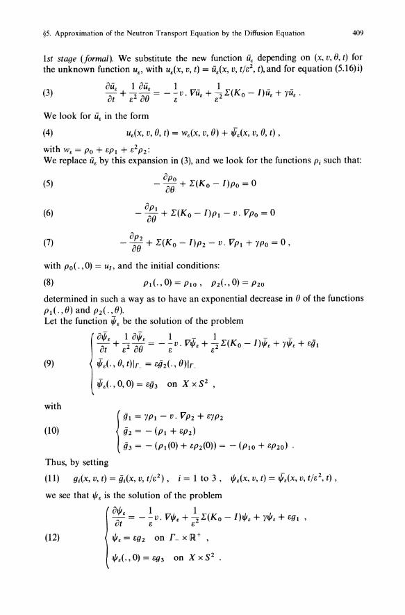
§5. Approximation of the Neutron Transport Equation by the Diffusion Equation 409
1st stage (formal). We substitute the new function ii, depending on (x, v, e, t) for the unknown function U,' with u,(x, v, t) = ii,(x, v, t/e2, t),and for equation (5.16)i)
oii, 1 oii, 1 _ 1 __ -;- + 2 ~e = - -v. VUE + 2L(Ko - I)u, + yu,. ut I', u I', I',
(3)
We look for ii, in the form
(4) u,(X, v, e, t) = w,(x, v, e) + "',(x, v, e, t) ,
with w, = Po + epi + e2p2: We replace ii, by this expansion in (3), and we look for the functions Pi such that:
(5) opo - ae + L(Ko - I)po = °
(6) OPI - ae + L(Ko - I)PI - V. Vpo = °
(7) OP2 - ae + L(Ko - I)P2 - V. VPI + YPo = 0,
with Po(., 0) = UI, and the initial conditions:
(8) PI (., 0) = PIO, pz(" 0) = P20
determined in such a way as to have an exponential decrease in e of the functions PI(.,e) and P2(.,e). Let the function i[J, be the solution of the problem
A"', 1 oi[J, 1 - 1 - - _ --;- + 2-;-e = - -v. Vt/J, + 2L(Ko - I)t/J. + yt/J, + egl ut I', u I', I',
(9) i[J.(., e, t)IL = elh(·, e)IL
i[J.(.,O,O)=e{h on XxS z ,
with
(10)
Thus, by setting
{ gl = YPI - V. Vpz + eYP2
gz = - (PI + epz)
{h = - (PI (0) + epz(O)) = - (PIO + ep20) .
(11) gi(X, v, t) = iMx, v, t/e Z ) , i = 1 to 3, t/J.(x, v, t) = ",.(x, v, t/ez, t) ,
we see that t/J. is the solution of the problem
ot/J. 1 1 --;- = - - v. Vt/J, + 2 L(Ko - I)t/J. + yt/J. + egl , ut I', I',
(12) t/J, = eg 2 on r _ x ~ + ,
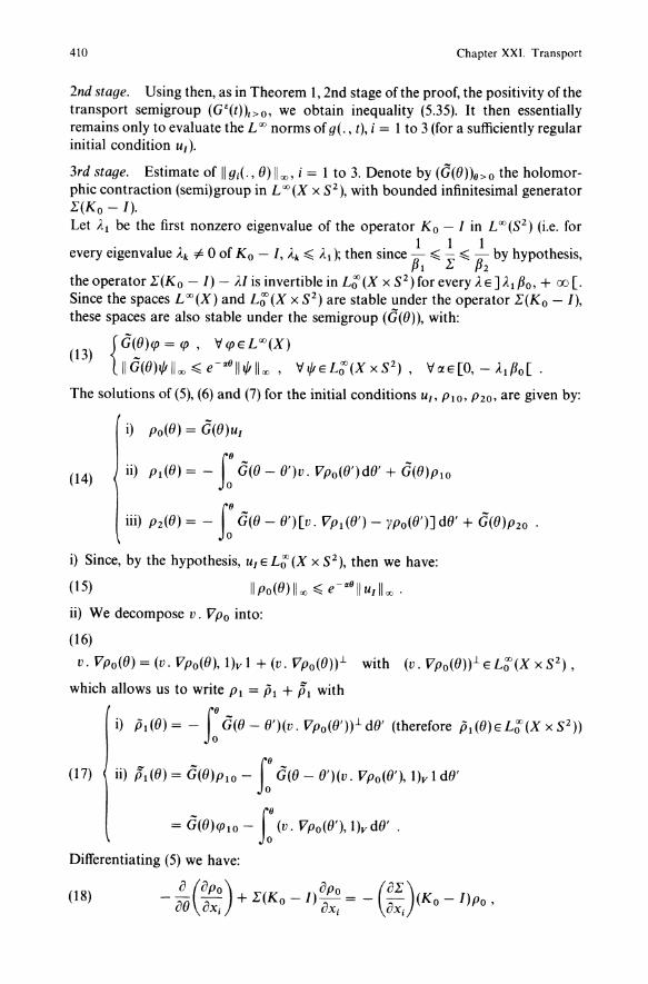
410 Chapter XXI. Transport
2nd stage. Using then, as in Theorem 1, 2nd stage ofthe proof, the positivity ofthe transport semigroup (G'(t))r>o, we obtain inequality (5.35). It then essentially remains only to evaluate the L 00 norms of g(. , t), i = 1 to 3 (for a sufficiently regular initial condition Ul)'
3rd stage. Estimate of Ilg;(., 0)1100' i = 1 to 3. Denote by (G(0))8> 0 the holomorphic contraction (semi)group in L 00 (X X S2), with bounded infinitesimal generator 1:(Ko - I). Let Al be the first nonzero eigenvalue of the operator Ko - I in L 00(S2) (i.e. for
. f . 1 1 Ib h h' every eIgenvalue Ak #- 0 0 Ko - I, Ak ~ AI); then SInce -P ~ - ~ -P y ypot eSIs, 1 1: 2
the operator 1:(Ko - I) - AI is invertible in L:f (X x S2) for every A E] Al Po, + 00 [.
Since the spaces L oo(X) and L:f(X x S2) are stable under the operator 1:(Ko - I), these spaces are also stable under the semigroup (G(O)), with:
{G(O)lfJ=lfJ, VlfJELoo(X)
(13) IIG(O)I/Illoo ~ e-«811 1/1 1100 , VI/IEL:f(XxS 2) , VtxE[O, - AIPo[ .
The solutions of (5), (6) and (7) for the initial conditions Ufo PI0, P20, are given by:
i) Po(O) = G(O)Ul
(14) ii) Pl(O) = - f: G(O - O')v. Vpo(O')dO' + G(0)PI0
iii) P2(0) = - f: G(O - O')[v. VPl(O') - YPo(O')] dO' + G(0)P20 .
i) Since, by the hypothesis, Ul E L:f (X x S2), then we have:
(15)
ii) We decompose v. Vpo into:
(16)
v. VPo(O) = (v. Vpo(O), l)v 1 + (v. VPo(O)).l with (v. VPo(O)).l E L:f(X X S2) ,
which allows us to write PI = PI + PI with
i) Pl(O) = - f: G(O-O')(v. VPo(O')).ldO' (therefore Pl(0)EL:f(XxS2))
(17) ii) PI (0) = G(O)PlO - f: G(O - O')(v. Vpo(O'), l)v 1 dO'
= G(O)lfJlo - f: (v. Vpo(O'), l)v dO' .
Differentiating (5) we have:
(18) a (opo) opo (01:) - 00 OX; + 1:(Ko - /) OX; = - OX; (Ko - /)po ,
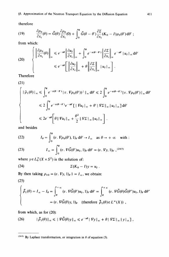
§5. Approximation of the Neutron Transport Equation by the Diffusion Equation 411
therefore
(19) 0:0 (0) = G(O) 0;0 (0) + I8 G(O - 0') ~I' (Ko - I)po((J') dO' ; u~ u~ 0 u~
from which:
(20) 11~:(O)t ~ e-~811~::t + f: e-~(8-8')II~~t e-~8'llullloodO'
~ e-~8[1I~::t + 0ll~~t IIUlll oo ] .
Therefore
(21)
Ilpl(O)lloo ~ f: e-~(8-8·)llv. VPo(O'))1-lloodO' ~ 2 f: e-~(8-8·)llv. VPo((J')IIoodO'
~ 2 f: e-~(8-8')e-~8'[1I VUlii oo + 0'11 VI'lloollulllooJdO'
~ 2e-~8[OII VUliioo + 022
11 VI'llooIIUlll oo ] .
and besides
(22) 18 = f: (v. Vpo((J'), l)y dO' ~ 100 as 0 ~ + 00 with:
(23) 100 = f: (v. VG(O')uJ, l)ydO' = (v. Vy, l)y ,(265)
where yeL;'(X x S2) is the solution of:
(24) I'(Ko - I)y = Ul .
By then taking PIO = (v. Vy, l)y 1 = 100 , we obtain:
(25)
ii, (0) ~ 1. - 1. ~. ~. VG(O')u" l)y dO' ~ .' (". VG(O) G( O")u" l)y dO" { f+oo f+oo
= (v. VG(O)y, l)y (therefore Pl(O)eLOO(X)) ,
from which, as for (20):
(26) II Pl(O) II 00 ~ II VG(O)Ylloo ~ e-~811 VYlloo + Oil VI'liooIlYllooJ,
(265) By Laplace transformation, or integration in (J of equation (5).
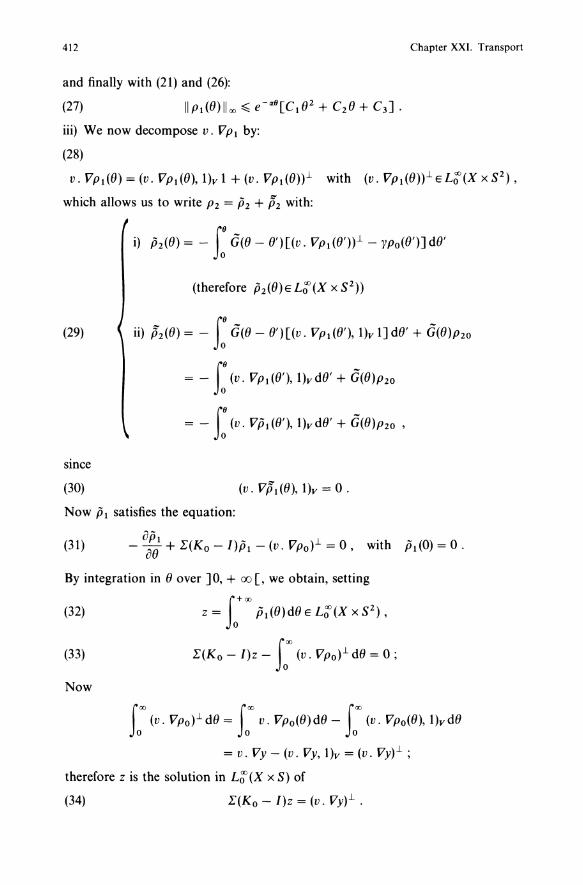
412 Chapter XXI. Transport
and finally with (21) and (26):
(27)
iii) We now decompose v. VPl by:
(28)
v. VpdO) = (v. VpdO), 1)y 1 + (v. VpdO))-L with (v. VP1(O))-L EL;'(X X SZ),
which allows us to write pz = pz + pz with:
i) pz(O) = - r G(O - e')[(v. Vpde'»-L - YPo(O')] de'
(therefore Pz(O)EL;'(XxSZ))
(29) ii) pz(O) = - f: G(O - O')[(v. Vpde'), 1)y 1] dO' + G(O)pzo
= - r (v. VpdO'), 1)ydO' + G(O)pzo
= - f: (v. VPl (0'), 1)y dO' + G(O)pzo ,
since
(30)
Now Pl satisfies the equation:
(31) apl _ -L - ae + 1:(Ko -l)Pl - (v. Vpo) = 0, with Pl(O) = o.
By integration in 0 over ]0, + 00 [, we obtain, setting
(32) f+oo Z = 0 Pl(O)dO E L;'(X x SZ) ,
(33) 1:(Ko - I)z - too (v. VPo)-L dO = 0 ;
Now
too (v. Vpo)-LdO= too v. VPo(O)dO- fooo (v. VPo(O), 1)ydO
= v. Vy - (v. Vy, 1)y = (v. Vy)-L ;
therefore z is the solution in L;'(X x S) of
(34) 1:(Ko - l)z = (v. Vy)-L .
§5. Approximation of the Neutron Transport Equation by the Diffusion Equation 413
By taking P20 = (v. Vz, l)v 1, we obtain
(35)
It remains to evaluate Ilp2(0)1I<x" IIp2(0)1I00 and for this II VPl(O) 1100 and
II a~: ~:Joo' which is done by successively differentiating (31) with respect to Xi,
then (5) with respect to Xi and Xj, and by using Picard's formula (see Chap. XVII B). We therefore obtain, denoting by Pn «(}) various polynomials of degree n in 0
(36)
To evaluate t/I. we must evaluate (g;), i = 1 to 3, and for this it is sufficient here to estimate v. V P2. Continuing as before, we obtain
(37)
from which
(38) 1191(., 0)1100 ~ e- IZ9 p s(0) , 1192(.' 0)1100 ~ e- IZ9 p 4 (0).
4th stage. We use inequality (5.35) with the estimates (38) and the initial value:
(39) 93 = - (PlO + 8P20) = - (v. V(y + 8Z), l)v ,
where y and ZE L;'(X x S2) are obtained by (24) and (34). We thus have
(40) II t/I.(., t) II 00 ~ ee61 II g311 00 + 8 f~ e 6(I-s{e - IX~ Ps CS2 ) ] ds ,
and hence, finally (with R constant),
(41) IIt/I.(.,t)lloo ~ 8e61 R.
By now taking w(., 0) = PoCO), we finally obtain, as a consequence of the inequalities deduced from (4), (11):
{ U.(X, v, t) = u.(x, v, t/82, t) = w.(x, v, t/8 2) + ",.(x, v, t/82, t)
(42) = w(x, v, t/82) + 8Pl (x, v, t/82) + 82 P2(X, v, t/82) + t/I.(x, v, t) .
From which, with (27), (36) and (41):
! lIu.(.,., t) - w(.,., t/82) II 00 ~ 8[lIpl(.,., t/82) II 00
(43) + ellp2(.,., t/e 2 ) 1100] + II t/I.(. , ., t)lloo
~ ee"'[e-(<l+~)p(t/e2) + R ] ~ 8e"'C ,
with C constant. Moreover we note that, from (15):
(44) Ilw(.,., t/82) II 00 ~ e-IX,/e21IurII00,
therefore for t ~ to > 0, lim II w(., ., t/82) II 00 -+ 0 for fixed t (t ~ to); w is sometimes .-+0
414 Chapter XXI. Transport
called the transitory term in neutron physics, and denoted by u tr (see §4). We must assume for the third stage that u/ is sufficiently regular and more precisely that u/ is a bounded function of X x S2, such that
D
2. Proof of Lemma 4. (The Golse-Perthame-Sentis compactness lemma [1])
We shall prove this lemma (and also a slightly stronger result) with the help of two other lemmas. For every u E WP(IR" x V), set:
(45) u(x) = Iv u(x, v)dJl(v) .
Let, for all a > 0, yE IR; = IR"\ {O},
(46) Ea,y = rYE V; Iv.YI > alyl}, E~,y = V\Ea,y = {VE V; Iv.yl:;:;; alyl} ;
E~,y is therefore the set of velocities whose orthogonal projection on the y-axis is inside the band limited by the two planes {VEIR", v.y/lyl = ± a}. We assume that Jl and V satisfy the condition:
(47) there exists a constant K > 0 such that: Jl(E~,y) < Ka V y E IR; (266) .
This condition is fulfilled in particular if V is bounded and Jl is the Lebesgue measure over V, or if the surface measure if V is a sphere.
Lemma 1. We assume V is compact c IR" and Jl satisfies (47). Let
(48) fi' = rUE W2(1R" x V), Ilullw':;:;; 1}; ff = {u given by (45), uEfi'} .
Then the set ff is such that ff Ix is relatively compact in L 2(X) for every open bounded set Xc IR".
Proof (Golse-Perthame-Sentis). It is sufficient to prove (see Brezis [1], p. 74) that:
{V £ > 0, 3 b > 0 such that
(49) IILhU-uIIL'(IR")<£, VhEIR" with Ihl<b, VUEfi'
(with LhU(X) = u(x + h)). Now, denoting by {i the Fourier transform of u:
(50) II LhU - u Ili'(IR") = r leihY{i(y) - {i(y)1 2 dy = r 4sin 2(hy/2)1{i(y)1 2 dy; JIR" JIR"
but, denoting by lEo., and IE:., the characteristic functions of Ea,y and E~,y, we have:
1{i(yW = I Iv u(y, V) dJl I2
= I Iv u(y, v)(I E;., + lEo)dJll2
:;:;; 2Jl(E~,y) Iv lu(y, v)1 2dJl + 2Jl(V) Iv lu(y, vW l Eo ,dJl.
(266) With, moreover, the usual condition that To c ax x V is of zero measure for dy dJl (see §2).
§5. Approximation of the Neutron Transport Equation by the Diffusion Equation 415
F h· h' 21' h. y 1 h Iv. yl rom w IC ,SInce SIn- ~ I .yl ~ Ihllyl ~ Ihl--, VVEEa Y' 2 rx'
(51) II 'hU - U Ili2(1R") ~ 8Krxll u Ili2(1R" x V) + 21l(V) Ih~2 II v. VU II i 2(1R" x V) • rx
Taking rx = IhI2/3 , we obtain
(52) II 'h U - U II i 2(1R") ~ K' I h 12/3 11 u II fy2(1R" x V), K' constant.
Hence we have Lemma 1. o Lemma 2. Let X be an open convex set oflRn and Va compact set oflRn. Thenfor all p E [1, + ex) [, there exists a continuous extension P: WP(X x V) --+ WP(lR n x V), with:
WP(X x V) = {UE WP(X X V), ulr± EU(r±, Iv.vldydll).
This lemma generalises easily to a finite family of convex, disjoint open sets (XdiEI such that d(Xi' XJ > 0, V i and j.
Proof For every point (x, V)EOX x V, the "time of travel" in XC = IRn\X, ,C(x, v) is infinite, and therefore by the trace theorems (see appendix of §2), the trace mapping u E WP(X C x V) --+ U Ir is continuous and surjective over the space U(r, I v. nl dy dll)(with r = ax x V), with continuous lifting. As the space oftraces of WP(X x V) is contained in U(r, I v. n I dy dll) by definition, we immediately deduce Lemma 2. The combination of Lemmas 1 and 2 implies the compactness lemma: 0
Lemma 3. Let X be an open bounded convex set oflRn, 11 a positive Radon measure over W, with compact support V satisfying (47). Then the set #x = {u with (45) and u E W2(X X V)} is relatively compact in L 2(X), and the mapping u --+ U is compact from W(X x V) into L2(X).
Corollary 1. Under the hypotheses of the compactness Lemma 3, we assume, that the functionfis such that fE rt!°(X, L2(VX V)); then the collision operator K given by:
Ku(x, v) = tf(X, v', v)u(x, v')dll(V')
is compact from wi (X x V)(267)(268) into L 2(X x V), and therefore K is a compact perturbation of the operator B = - v. V - 1: (with 1: E L 00 (X x V)), D(B) = wi (X x V) and the essential spectra of T = B + K and B are identical: "e(T) = "e(B).
Proof 1) We first of all remark that (with the notation dv for dll(V)):
Ilullfy2 = Ilulli2 + Ilv. Vulli2 ~ Ilulli2,
(267) With, recall W;(X x V) = {uEL2(X x V), v. VUEL2(X x V), ulr_ = O}. (268) Or more generally from W2(X x V) = {UE W2(X x V), uk E L 2(T, Iv. nl dy dJl)}.
416 Chapter XXI. Transport
and:
II Ku 1112(x x V) = Ix x v dx dv I Iv f(x, v', v) u(x, v') 12 dv'
~f dXdvf If(X'V',V) 12 dv'f lu(x,v')1 2dv' Xx v v v
~f dXf If(X,v',vWdVdv'f lu(x,v'Wdv' x Vx v v
~ [SUp f If(x, v', vW dVdV'] \I u 1112(X x V) • x Vx V
Therefore K is a continuous operator in L 2(X x V), satisfying:
II K 11:e(W~,L2) ~ II K 11:e(L2 ) ~ (sup f If(x, v', v)1 2 dVdv,)l!2 x Vx V
2) Since fErtf°CX, L2(VX V)), then (by a Weierstrass type theorem) f can be approximated uniformly by linear combinations (with coefficients in L 2(X x V)) of rtf 1 (X, \R) functions, and consequently:
k. f= limr inrtf°(X,L2(VxV)), with r(x, v', v) = I g;n(V)lfJ;(X,v')
n~oo ; = 1
where g,/ E L 2(V), lfJ? are regular enough for the multiplication mapping u --+ lfJ;U to be continuous in wi (X x V). 3) Then, on the one hand, the collision operators K n, such that
Knu(x, v) = Lr(x, v', v)u(x, v')dv' ,
are compact from wi (X x V) into L 2(X x V), since the mappings
0' Wi(Xx V) ~ Wi(Xx V) ~ L2(X)~ L2(XX V)
u ;;;;;: = L lfJ;nu(x, v')dv' --+ Uu
are compact (being composed of bounded mappings and the compact mapping -), and on the other hand they are also convergent in norm to the operator K which is therefore compact from wi (X x V) into L 2(X x V). 0
We therefore recover directly the spectral results stated in §3 - See in particular Theorems 3 and 4, §3 - from Propositions 1 to 3, §3.