Lecture notes for

Mathematical Cell Biology

Christian Schmeiser1

1 Introduction

The cell could serve as the basis for a definition of life on earth, at least froma practical if not from a philosophical point of view. It is often called thebasic unit of life, since it is a building block of all living beings. Consideringthe enormous variety of life on earth, it is by no means obvious that it makessense to talk about the cell. This can be motivated by the astonishing factthat all different cell types share a number of basic properties hinting to avery small number of common ancestors. For these reasons, cell biology isnot just an ever growing collection of (unrelated) facts about cells, but ascientific field with a large common basis and with systematic approachesto extending our knowledge. Cell biology explains the structure and organi-zation of cells, their physiological properties, metabolic processes, signalingpathways, life cycle, and interactions with their environment. Knowing thecomponents of cells and how cells work is fundamental to all biological sci-ences.

The strongly related field molecular biology concentrates on detailedchemical aspects. Biochemistry is characterized by the occurrence of onlya small number of elements, which are however combined into sometimesvery large molecules. The 4 most common elements carbon (C), hydrogen(H), nitrogen (N), and oxygen (O) make up for about 96.5% of the massof a cell, with the rest provided mostly by the less common elements cal-cium (Ca), chlorine (Cl), magnesium (Mg), phosphorus (P), potassium (K),sodium (Na), and sulfur (S). The molecules in cells are mainly water (appr.85%), lipids (fat molecules), and proteins (large molecules responsible forall cell activities). The information about the cell identity is stored in thedesoxyribonucleic acid (DNA). Parts of this information are distributed andused in the cell via ribonucleic acids (RNA).

Cells are divided into two main categories: prokaryotes and eukaryotes.The main difference is that prokaryotes do not have a nucleus and a much

1Institut fur Mathematik, Universitat Wien, Oskar-Morgenstern-Platz 1, 1090 Wien,Austria. christian.schmeiser@univie.ac.at

1

Figure 1: some of the most important organelles of animal cells

simpler internal organisation. This category contains archaea and bacteria,both unicellular organisms, whereas eukaryotic cells occur in animals, plants,fungi, and protista (or protozoa). Animals, plants, and fungi are multicellu-lar with sometimes huge numbers of cells per individual (3.72× 1013 for theaverage human adult, according to an estimate published in 2013 [2]). Cellbiology focuses more on the study of eukaryotic cells than on prokaryotes,which are covered in the field of microbiology. Eukaryotic cells have sepa-rated compartments called organelles, serving well defined functions. In thefollowing we list some of them (see also Fig. 1):

Centrosome: an associated pair of cylindrical shaped protein structures(centrioles) that organize microtubules.

Cell membrane (plasma membrane): the part of the cell which sepa-rates the cell from the outside environment as well as cellular compart-ments from each other. It also contributes to the regulation of cellularprocesses.

Cell wall: extra layer of protection and gives structural support (only foundin plant cells).

Chloroplast: key organelle for photosynthesis (only found in plant cells).

2

Cytoplasm: contents of the main fluid-filled space inside cells, where manychemical reactions happen.

Cytoskeleton: protein filaments inside cells (microfilaments, microtubules,and intermediate filaments), serves several functions, such as cell shapechanges, cell movement, intracellular transportation and signaling.

Endoplasmic reticulum (rough): major site of membrane protein syn-thesis.

Endoplasmic reticulum (smooth): major site of lipid synthesis.

Golgi apparatus: distribution system for proteins.

Lysosome: acidic organelle that breaks down cellular waste products anddebris into simple compounds (only found in animal cells).

Mitochondrion: power plant of the cell, storing energy in Adenosin triphos-phate (ATP).

Nucleus: contains chromosomes composed of DNA

Ribosome: RNA and protein complex required for protein synthesis in cells

Vesicle: small membrane-bounded spheres inside cells

Theoretical cell biology tries to explain cellular mechanisms in terms ofchemical and/or mechanical processes. It typically suffices to use a standardstochastic description of chemical reactions and classical (i.e. Newtonian)mechanics. Such explanations can be formulated in terms of mathematicalmodels. The formulation of these models, their solution, and the biologicalinterpretation of model properties make up the field of mathematical cellbiology, the subject of this course, which covers only a small section of thisrapidly growing field.

2 Mathematical models for chemical reactions

Chemical substances might be very unevenly distributed in cells with strongeffects on reactions between them. For simplicity we shall start, however,assuming a well mixed reactor, where it suffices to describe the substancesX1, . . . , Xn by their concentrations c(t) = (c1(t), . . . , cn(t)) at time t, mea-sured in numbers of molecules per volume.

3

The concentrations change with time as the consequence of m chemicalreactions with the reaction rates r(t) = (r1(t), . . . , rm(t)) and the stoichio-metric coefficients νij ∈ ZZ, i = 1, . . . , n, j = 1, . . . ,m. The reaction ratesdescribe, how many times per volume and per time a reaction takes place.The stoichiometric coefficients describe the book keeping: When νij > 0,each occurrence of reaction number j produces νij molecules of the substanceXi. Whereas for νij < 0 each occurrence of reaction number j destroys −νijmolecules of the substance Xi. For νij = 0 the substance Xi is not involvedin reaction number j. The stoichiometric matrix is given by

N =

ν11 · · · ν1m...

...νn1 · · · νnm

.

The model for the evolution of the concentrations is the ODE system

dc

dt= Nr .

For so called simple reactions, the reaction rates can be modeled by themass action law

rj = kj∏

i: νij<0

c−νiji , j = 1, . . . ,m ,

with the reaction constants kj > 0. The product contains a factor ci foreach molecule of Xi entering the reaction. The total number

−∑

i: νij<0

νij

of these molecules is called the order of the reaction. For given reaction con-stants and stoichiometric coefficients, the concentrations can be computed,when also initial conditions

ci(0) = ci0 , i = 1, . . . , n ,

for the concentrations are prescribed. Since we have assumed time indepen-dence of the data, the choice t = 0 for the initial time does not mean a lossof generality.

4

A simple example: Let us consider the reaction X1 +X2 → X3 and itsreverse with the stoichiometric matrix

N =

−1 1−1 11 −1

.

Thus, we have the rates r+ = k+c1c2 for the second order forward reactionand r− = k−c3 for the first order reverse reaction, leading to the ODEs

dc1

dt= k−c3 − k+c1c2 ,

dc2

dt= k−c3 − k+c1c2 ,

dc3

dt= k+c1c2 − k−c3 ,

subject to initial conditions

c1(0) = c10 , c2(0) = c20 , c3(0) = c30 .

We can use the conservation laws

dc1

dt− dc2

dt= 0 and

dc1

dt+dc3

dt= 0 ,

and their consequence

c2(t) = c1(t)− c10 + c20 , c3(t) = −c1(t) + c10 + c30 ,

to reduce the system to the scalar equation

dc1

dt= f(c1) , mit f(c1) = k−(c10 + c30)− c1(k− + k+c20 − k+c10)− k+c

21 ,

which possesses a unique, positive, asymptotically stable equilibrium.

A zeroth order reaction: Now we consider X1 → X2 and the reversereaction (both first order), leading to the initial value problem

dc1

dt= k−c2 − k+c1 ,

dc2

dt= k+c1 − k−c2 , c1(0) = c10 , c2(0) = c20 .

We assume that the reverse reaction has a much smaller reaction constant,i.e. k− k+. The reaction rates can only by of the same order of magni-tude, if c1 is much smaller than c2, which we assume for their initial values:c10 c20. We shall analyse the consequences of these assumptions by anappropriate scaling. In particular, we shall use intrinsic reference quantities,i.e. units for the variables computed from the parameters of the problem.

5

We choose the initial values for the concentrations and 1/k+ for time.This means to introduce the transformations

u1(τ) =c1(τ/k+)

c10, u2(τ) =

c2(τ/k+)

c20,

where u1, u2, and τ are the dimensionless quantities. This leads to

u′1 =u2

a− u1 , u′2 = ε(au1 − u2) , u1(0) = u2(0) = 1 , (1)

with the dimensionless parameters ε 1 and a (assumed of moderate size),defined by

k−k+

= ε ,c10

c20= εa .

The limit ε→ 0 gives the approximation u2(τ) = 1 for τ ≥ 0 and

u′1 =1

a− u1 , u1(0) = 1 .

The rate of the reverse reaction is approximated by 1/a, which is calleda zeroth order reaction. The substance X2 is taken from a big reservoir,approximately uneffected by the reaction.

Michaelis-Menten-Kinetics: Assume the enzyme E controls a reaction,where the substrats S is transformed to the product P . This happens intwo partial reactions, where enzyme and substrate first build the complexES, which is then decomposed into the product and the unchanged enzyme,i.e. E + S → ES → P + E. We assume that initially there is only enzymeand substrate with a much smaller enzyme concentration. This leads to theinitial value problem

c′S = −k1cEcS , cS(0) = cS0 ,

c′E = k2cES − k1cEcS , cE(0) = cE0 ,

c′ES = k1cEcS − k2cES , cES(0) = 0 ,

c′P = k2cES , cP (0) = 0 .

We introduce the scaling uS = cS/cS0, uP = cP /cS0, uE = cE/cE0, uES =cES/cE0, and τ = k1cE0t:

u′S = −uEuS , uS(0) = 1 ,

ε u′E = a uES − uEuS , uE(0) = 1 ,

ε u′ES = uEuS − a uES , uES(0) = 0 ,

u′P = a uES , uP (0) = 0 , (2)

6

with the dimensionless parameters

ε =cE0

cS0 1 , a =

k2

k1cS0.

Adding the second and the third differential equation gives the conservationlaw

uE(τ) + uES(τ) = 1 .

This and the limit ε→ 0 in the second equation lead to 0 = a(1−uE)−uEuSand, thus,

uE(τ) =a

a+ uS(τ). (3)

The result is a direct reaction rate for S → P :

u′P = −u′S =a uSa+ uS

,

or, in terms of the original unscaled variables,

c′P = −c′S =k1k2cE0cSk2 + k1cS

.

This result is called Michaelis-Menten kinetics [7]. It can be seen as aninterpolation between a first order reaction (rate ≈ k1cE0cS) for small valuesof cS and a zeroth order reaction (rate ≈ k2cE0) for large values of cS .

The system (4) is called singularly perturbed, as opposed to the regu-larly perturbed system (1), because two of the differential equations becomealgebraic equations in the limit ε→ 0. Note that in the limit, the approxi-mations for the fast variables uE = a/(a+uS) and uES = uS/(a+uS) cannotsatisfy the correct initial conditions, whereas the initial values for the ap-proximations of the slow variables uS and uP can be chosen appropriately.The solution to this dilemma is to consider the fast time scale σ = τ/ε. Interms of this new variable, the problem takes the regularly perturbed form

duSdσ

= −εuEuS , uS(0) = 1 ,

duEdσ

= a uES − uEuS , uE(0) = 1 ,

duESdσ

= uEuS − a uES , uES(0) = 0 ,

duPdσ

= εa uES , uP (0) = 0 , (4)

7

The limit ε→ 0 now leads to the initial layer approximation

uE =a+ e−σ(1+a)

a+ 1, (5)

whose limit a/(a+1) as σ →∞ coincides with the value of the approximation(3) for τ = 0, a matching relation in the language of singular perturbationtheory.

First order weakly reversible systems: We consider reaction networkswith only first order reactions of the form Xi → Xj with reaction constantkij ≥ 0, i, j = 1, . . . , n, i 6= j. It is useful to represent the network as adirected graph with nodes Xi, i = 1, . . . , n, and an edge directed from Xi toXj , iff kij > 0. The ODE system modeling the network is

dcidt

=∑j 6=i

(kjicj − kijci) , i = 1, . . . , n, (6)

with initial condition ci(0) = ci,0 ≥ 0, i = 1, . . . , n. Since, obviously,

n∑i=1

dcidt

= 0 ,

the total number of molecules is conserved:

n∑i=1

ci(t) =

n∑i=1

ci,0 =: M , t ≥ 0 .

It is also easily seen that ci(t) ≥ 0 for i = 1, . . . , n, t ≥ 0 is a consequence ofthe nonnegativity of the initial data. The dynamics is therefore restrictedto a compact subset of a hyperplane.

We pose the question of the existence of a positive equilibrium (c1,∞, . . . , cn,∞),where positive means that all concentrations are positive: ci,∞ > 0, i =1, . . . , n. Considering for a moment the case n = 2 shows that we needeither k12, k21 > 0 or the trivial case k12 = k21 = 0. For n > 2 the situationis more complicated.

Definition 1 A directed graph is weakly reversible, iff for every edge Xi →Xj it contains a path Xj → Xi1 → . . .→ Xir → Xi.

8

Lemma 1 Let the directed graph corresponding to (6) be connected andweakly reversible, and let M > 0. Then there exists a unique positive equi-librium with total concentration M , i.e. there exists (c1,∞, . . . , cn,∞) with∑

j 6=i(kjicj,∞ − kijci,∞) = 0 , ci,∞ > 0 , i = 1, . . . , n , (7)

n∑i=1

ci,∞ = M .

For a proof see [4]. We claim that, in the situation of the Lemma,

L(t) =1

2

n∑i=1

ci,∞ui(t)2 , with ui(t) =

ci(t)− ci,∞ci,∞

is a Lyapunov function:

dL

dt=

n∑i=1

∑j 6=i

ui(kjicj − kijci) =n∑i=1

∑j 6=i

ui (kji(cj − cj,∞)− kij(ci − ci,∞))

=n∑i=1

∑j 6=i

ui (kjicj,∞uj − kijci,∞ui) ,

where, for the second equality, we have used the equilibrium property (7).For the second term, we derive two different representations:

n∑i=1

∑j 6=i

kijci,∞u2i =

∑j 6=i

kjicj,∞u2j and

n∑i=1

∑j 6=i

kijci,∞u2i =

∑j 6=i

kjicj,∞u2i ,

where the first follows from i↔ j and the second again from (7). Using halfof each of these, we get

dL

dt=

n∑i=1

∑j 6=i

kjicj,∞

(uiuj −

1

2u2i −

1

2u2j

),

= −1

2

n∑i=1

∑j 6=i

kjicj,∞ (ui − uj)2 ≤ 0 .

Not only is L a Lyapunov function, but under the assumptions already made,the right hand side above can be shown to be negative definite.

9

Lemma 2 Under the assumptions of Lemma 1 there exists γ > 0 such that

n∑i=1

∑j 6=i

kjicj,∞ (ui − uj)2 ≥ γn∑i=1

ci,∞u2i ∀ (u1, . . . , un) ∈ IRn .

A proof can again be found in [4]. This implies the differential inequality

dL/dt ≤ −γL , (8)

and, with the Gronwall lemma (see below),

L(t) ≤ e−γtL(0) .

Theorem 1 Under the assumptions of Lemma 1 there exist α, γ > 0 suchthat

|ci(t)− ci,∞| ≤ αe−γt/2 , i = 1, . . . , n .

Concerning the Gronwall lemma, we first state that (8) implies

L(t) ≤ L(τ)− γ∫ t

τL(s)ds , 0 ≤ τ ≤ t . (9)

Lemma 3 (Gronwall, decaying) Let L ∈ C([0,∞)) satisfy L(t) ≥ 0 and(9) with γ ≥ 0. Then

L(t) ≤ e−γtL(0) , t ≥ 0 .

Proof: Assume there exists t∗ > 0, such that L(t∗) > e−γt∗L(0) =: L(t∗).

Lett := maxt ∈ [0, t∗) : L(t) = L(t) ,

i.e. L(t) = L(t) and

L > L in (t, t∗] . (10)

We also define

ϕ(t) = L(t)− γ∫ t

tL(s)ds .

Then ϕ(t) = L(t) and

d

dt(ϕ/L) =

γ(ϕ− L)

L≥ 0

10

by (9). This implies ϕ ≥ L in [t, t∗], which is equivalent to∫ t

tL(s)ds ≤

∫ t

tL(s)ds , t ∈ [t, t∗] .

This is a contradiction to (10).

The above result is an extension [10] of the classical Gronwall lemma(in integral form) for exponentially growing bounds, which needs a weakerassumption and is easier to prove:

Lemma 4 (Gronwall, growing) Let L ∈ C([0,∞)) satisfy L(t) ≥ 0 andL(t) ≤ L(0) + γ

∫ t0 L(s)ds, t ≥ 0, with γ ≥ 0. Then

L(t) ≤ eγtL(0) , t ≥ 0 .

Proof: The function

v(t) := e−γt∫ t

0L(s)ds

satisfiesdv

dt(t) = e−γt

(L(t)− γ

∫ t

0L(s)ds

)≤ e−γtL(0) .

By integration we obtain

v(t) ≤ L(0)

γ

(1− e−γt

).

Since L(t) ≤ L(0) + γeγtv(t), the result follows. Note that γ ≥ 0 is used inthis last step.

3 Random motion of atoms and molecules

Atoms and molecules in cells live in a complex nonhomogeneous environmentinfluencing their movement. As a consequence, for an observer this move-ment looks like having a random component. We therefore accept a randomnature of this movement as a postulate for a mathematical description.

We start by approximating this movement by a jump process on a grid,and we first restrict to one spatial dimension for simplicity. Let xj = j∆x,j ∈ ZZ, denote the possible positions of particles, and assume that at thediscrete points tn = n∆t, n ∈ ZZ, in time particles perform jumps of the

11

length ∆x to the left or to the right. Let us assume further that the proba-bility of jumping to the left is q, and the probability of jumping to the rightis 1 − q (with 0 ≤ q ≤ 1, of course). Now we introduce the nonnegativequantities pnj , j, n ∈ ZZ, which can be interpreted either as the probabilitythat one particle is at the position xj at time tn or as the expected numberof particles out of a large ensemble at position xj at time tn or (if the latteris divided by ∆x) as the expected number density of particles at positionxj at time tn. Then, obviously the values at time tn+1 can be computed interms of the values at time tn:

pn+1j = qpnj+1 + (1− q)pnj−1 (11)

Eventually we are looking for continuous descriptions both in time and inposition. Therefore we shall interpret pnj as approximation for p(xj , tn)where p is a function of two real valued arguments. With this interpretationin mind we rewrite the above equation as

pn+1j − pnj

∆t− q∆x

∆t

pnj+1 − pnj∆x

+(1− q)∆x

∆t

pnj − pnj−1

∆x= 0 .

Our aim is to pass to the limit ∆x,∆t → 0. Obviously the result dependson the relative size of ∆x and ∆t. We have three main options: Either thegrid speed s := ∆x/∆t tends to zero, to infinity, or we keep it fixed at apositive finite value. The most interesting result occurs in the latter case,which we call the significant limit:

∂tp+ ∂x(vp) = 0 , with v = s(1− 2q) . (12)

Actually, the other two cases can be recovered by letting s→ 0 or s→∞.Equation (12) is a one-dimensional convection equation. Solutions are

travelling waves p(x, t) = f(x− vt) with velocity v. With the interpretationof p as time dependent density of particles along the line, the integratedversion of (12),

d

dt

∫ b

ap(x, t)dx+ vp(b, t)− vp(a, t) = 0 ,

gives the rate of change of the number of particles contained in the interval(a, b). The term j(x, t) = vp(x, t) can then be interpreted as the flux ofparticles through the point x at time t, and v is the mean velocity of particles.

It is interesting to note that equation (12) could have been derived with-out any probabilistic effects. The assumption that all particles always move

12

to the right or always to the left, i.e., q = 0 or q = 1, still leads to (12) withv = ±s. More generally, the same value of v, and therefore the same macro-scopic equation (12) can be obtained by different choices of the grid speed sand of the probability q. This shows that the properties of the microscopicmovement cannot be completely recovered from macroscopic observations.

In the symmetric situation q = 1/2, the mean velocity vanishes, and (12)becomes trivial. This unsatisfactory situation can be clarified by returningto the discrete equation (11) and by rewriting it in a different way:

pn+1j − pnj

∆t− (∆x)2

2∆t

pnj+1 − 2pnj + pnj−1

(∆x)2= 0 .

This shows that for q = 1/2, the significant limit is achieved, when D =(∆x)2/(2∆t) is kept fixed as ∆x,∆t→ 0:

∂tp−D∂2xp = 0 . (13)

This is the one-dimensional diffusion equation with diffusivityD. Integrationas above shows that the diffusive flux is given by Fick’s law j = −D∂xp.

So far we have seen that the macroscopic limit of a biased random motionis a convection equation, and for an unbiased motion it is a diffusion equa-tion. Actually, both effects can be combined in the macroscopic equationby an appropriate scaling assumption. We shall also generalize the positionjump process by allowing a dependence of the jump probability on positionand time:

pn+1j = qnj+1p

nj+1 + (1− qnj−1)pnj−1 .

As in the derivation of the diffusion equation we assume thatD = (∆x)2/(2∆t)is fixed and that the jump probabilities are close to 1/2:

qnj =1

2− v(xj , tn)∆t

2∆x,

where v(x, t) is a given velocity function. The analogous computations asin the derivation of the diffusion equation now lead to the one-dimensionalconvection-diffusion equation

∂tp+ ∂x(vp−D∂xp) = 0 . (14)

Everything we did so far can be extended to higher dimensions with theresult

∂tp+∇ · (vp−D∇p) = 0 , (15)

13

where now the density p(x, t) depends on position x ∈ IRd, with d = 2 ord = 3, and on time t ∈ IR. The gradient with respect to x is denoted by∇ and the divergence by ∇·. The velocity v(x, t) and the flux vp − D∇pare vector fields. The interpretation of the flux vector is the following: Itscomponent in the direction ν is the number of particles per time and perunit area moving through an area element orthogonal to ν. This can be seenby integrating (15) over a bounded position domain Ω ⊂ IRd and using thedivergence theorem:

d

dt

∫Ωp dx+

∫∂Ω

(vp−D∇p) · ν dσ = 0 , (16)

where ν denotes the unit outward normal vector along the boundary ∂Ω,and dσ is the line element for d = 2 and the surface element for d = 3.

So far we have only described the movement of particles. Equation (15)is a conservation law. No particles are created or destroyed. As the finalstep in this modelling section, we also allow for this possibility. We denoteby f(x, t) the number of particles created or destroyed (depending on thesign of f) per unit time and unit volume. Then the right hand side of (16)has to be replaced by the integral of f over Ω, and the differential version(15) becomes the reaction-convection-diffusion equation

∂tp+∇ · (vp−D∇p) = f . (17)

Why reaction? In a typical situation our particles are molecules whosecreation or destruction is the result of a chemical reaction.

In the following, systems of equations of the form (17) for different speciesof particles will be considered, when x varies in a domain Ω ⊂ IRd, repre-senting the whole cell or a cell compartment. Typically we shall use zeroflux boundary conditions

(vp−D∇p) · ν = 0 along ∂Ω .

For given v and f , the formulation of a well posed problem for the unknown pis completed by prescribing initial conditions p(x, 0) = pI(x) for x ∈ Ω, withgiven initial data pI . Well posedness means that the initial-boundary valueproblem has a unique solution continuously dependent (in an appropriatesense) on the data v, f , and pI .

4 Gene regulatory networks

The main source for the material of this section is [1].

14

DNA can be subdivided into genes, each of which contains a code iden-tifying a protein. The subject of this section is gene expression, which is(not exclusively, but mostly) the process of the production of these pro-teins. From an information point of view, a gene can be interpreted as aword written in a 4-letter-alphabet, where the letters are called adenine,cytosine, guanine, and thymine. Similarly a protein can be seen as a word,however written in a 20-letter-alphabet with amino acids as letters. Sohow are genes translated into proteins? It is an amazing fact that the an-swer is almost universal for all living species. It is called the genetic code.Each group of three letters of the gene, called a codon, uniquely determinesan amino acid. Since there are 43 = 64 different codons, there is a lot ofredundancy in the sense that several codons code for the same amino acid.

It is an obvious fact that each cell has to make decisions about howmuch of each protein is produced at each time. For example, in multicellularorganisms this determines the cell type. Gene regulation is the name for themechanisms for making these decisions.

The production of a protein typically requires two steps:

• Transcription is the process, where a copy of the gene, called mes-senger RNA (mRNA) is produced.

• Translation is the actual production of the protein in a ribosome, amolecular machine, using the mRNA as input.

Very often (but not exclusively) gene regulation affects the transcriptionprocess. Typically a molecule binds to a so called promotor site of a geneeither up- or down-regulating transcription. Accordingly, the molecule iscalled an activator or, respectively, a repressor. As a first step in the math-ematical modelling, we describe the binding and unbinding of activators andrepressors, reactions of the form F + mA → B, where m molecules of typeA bind to a free promotor site F , producing a bound promotor site B, andthe reverse reaction. Considering the molecule concentration cA(t) as given,the rules of Section 2 imply

dcBdt

= −dcFdt

= k1cF cmA − k2cB .

Assuming this process to be fast compared to the changes in cA (similar tothe Michaelis-Menten asymptotics), we obtain the quasi-stationary result

cB =c0(cA/c)

m

1 + (cA/c)m, cF =

c0

1 + (cA/c)m, (18)

15

with the conserved total number of promotor sites c0 = cB + cF and thecritical value c = (k2/k1)1/m for cA. The function

h(c; c,m) =(c/c)m

1 + (c/c)m,

sometimes called the Hill function, makes a transition from small values tovalues close to 1 around the critical value c = c. The transition becomessharper with bigger exponent m. Obviously, (18) can be written as

cB = c0h(cA) , cF = c0(1− h(cA)) . (19)

Big values of m are often used, not because there exists a correspondingmolecular theory, but because of the experimental observation of a rathersharp switching in gene regulation.

The next step is to model transciption, i.e. the production of mRNAwith concentration cM (t). We assume that both free and bound promotorsites contribute and that there is also spontaneous degradation:

dcMdt

= αF cF + αBcB − γMcM ,

with positive parameters αF , αB, and γM . With (19), the sum of the firsttwo terms on the right hand side is an increasing function of cA for αF < αB,and a decreasing function of cA for αF > αB. In the first case A is anactivator, and in the second case a repressor. Typically, αF and αB are ofstrongly different magnitudes, to produce a pronounced effect.

Finally, we use a simple model for translation, i.e. for the protein con-centration cP (t):

dcPdt

= αMcM − γP cP ,

where we assume that the process is not limited by the availability of ribo-somes or the necessary protein ingredients, and that there is also sponta-neous degradation of protein.

Negative feedback – homeostasis. As a simple example, we consider aprotein, which acts as a repressor for its own production. This leads to themodel

dcMdt

= f(cP )− γMcM ,

dcPdt

= αMcM − γP cP , (20)

16

with the strictly decreasing function

f(cP ) := αF c0 − (αF − αB)c0h(cP ) , αF > αB .

It is easily seen that there is a unique steady state (cM,∞, cP,∞) ∈ IR2+, since

the nullclines

cM =f(cP )

γM, cM =

γP cPαM

,

are the graphs of a strictly increasing and a strictly decreasing function witha unique intersection. Linearization shows that this steady state is locallyasymptotically stable.

It is also easily seen that every rectangle of the form

[0, cM,max]×[0,αMcM,max

γP

]with cM,max ≥ f(0)/γM is an invariant region for (20). Therefore everytrajectory starting with nonnegative initial values is bounded.

The function

L(cM , cP ) =αM2

(cM − cM,∞)2 +

∫ cP

cP,∞

(f(cP,∞)− f(c)) dc .

is a Lyapunov function, since

d

dtL(cM , cP ) = −αMγM (cM−cM,∞)2−γP (cP −cP,∞)(f(cP,∞)−f(cP )) ≤ 0 ,

where we have used that f is decreasing.The Lyapunov function is strictly convex, nonnegative, and takes its

unique minimum at (cM,∞, cP,∞). Similarly dL/dt only vanishes for (cM , cP ) =(cM,∞, cP,∞). Even better, by the boundedness of the trajectories, forevery such bounded solution there exists a constant κ > 0, such that|f(cP )− f(cP,∞)| ≥ κ|cP − cP,∞|, implying

L(cM (t), cP (t)) ≥ αM2

(cM (t)− cM,∞)2 +κ

2(cP (t)− cP,∞)2 .

So L controls the distance to the equilibrium. On the other hand, by themonotonicity of f ,∫ cP

cP,∞

(f(cP,∞)− f(c)) dc ≤ (cP − cP,∞) (f(cP,∞)− f(cP )) ,

17

implying

dL

dt≤ −αMγM (cM − cM,∞)2 − γP

∫ cP

cP,∞

(f(cP,∞)− f(c)) dc

≤ −γL , with γ = min 2γM , γP .

As a consequence of the Gronwall lemma, we have

L(t) ≤ L(0)e−γt

for t ≥ 0, i.e. exponential convergence of all solutions to the steady state.This self-regulation by negative feedback, such that the protein concen-

tration is kept at the constant level cP,∞ in a stable way, is an examplefor homeostasis. The fact that this protein level is in a sense optimal, isexpected to be a consequence of evolution.

Mutual inhibition – bistability We consider two proteins, inhibitingeach other. As a simplification we assume that the transciption dynamicsfor both proteins is much faster than the translation dynamics, and that themRNA densitites therefore can be approximated by quasi-stationary states.The result is a system for the protein densities. Furthermore we make anoften used simplifying assumption, which corresponds to letting the Hillexponents pass to infinity:

dc1

dt= f2(c2)− γ1c1 ,

dc2

dt= f1(c1)− γ2c2 , (21)

with

fj(cj) =

aj for cj < cj ,bj else,

aj > bj > 0 , j = 1, 2. (22)

Note that the discontinuity of fj takes us out of the standard theory forordinary differential equations, which requires Lipschitz continuity of theright hand side for existence and uniqueness of solutions. We shall make atheoretical detour to discuss this problem.

Filippov solutions of ODEs with discontinuous right hand side: As a firstexample, consider the ODE

du

dt= sign(u) . (23)

18

An obvious first question is for the value of the derivative, when u = 0. The answerof Filippov [5] is to replace the differential equation by a differential inclusion. Heredefines the sign function as set valued,

sign(u) :=

−1 for u < 0 ,[−1, 1] for u = 0 ,1 for u > 0 ,

(24)

and replaces (23) by

du

dt∈ sign(u) , for almost all t . (25)

The problem is that the uniqueness of solutions for initial value problems might getlost: The functions

u(t) = (t− t0)+ and u(t) = −(t− t0)+

are Filippov solutions of (25) with the initial condition u(0) = 0 for every value oft0 ≥ 0. This is, however, not necessarily the case:

−dudt∈ sign(u) , u(0) = u0 ,

has the unique Filippov solution

u(t) =

u0 − t sign(u0) for t < |u0| ,0 for t ≥ |u0| .

The uniqueness can be obtained as a consequence of sign(u) being the subdifferen-tial ∂|u| of a convex function [3], i.e. its monotonicity. This requirement can begeneralized to systems

du

dt∈ F (u) ,

where, for each u, F (u) ⊂ IRd is a convex set. However, requiring monotonicity is

too restrivtive, since it is not necessary in regions, where F can be represented by asmooth function. Filippov uses one-sided Lipschitz continuity: He shows uniquenessof Filippov solutions, if there exists a (one-sided Lipschitz) constant L ≥ 0, suchthat

(u1−u2) · (F1−F2) ≤ L|u1−u2|2 , for all u1, u2 and F1 ∈ F (u1) , F2 ∈ F (u2) .

For scalar equations this does not allow upward jumps of the right hand side.Actually, this is still too restrivtive for our purposes. It is easily seen that initialvalue problems for the differential inclusion

du

dt∈ 2 + sign(u) ,

19

have unique strictly increasing Filippov solutions. Their derivatives just jump from1 to 3, when they pass through u = 0. Obviously, the right hand side is not one-sided Lipschitz. We shall propose a uniqueness criterion adjusted to the situationof the system (21), (22), where the right hand side has jump discontinuities acrosshypersurfaces.

Let the domain B ∈ IRd be the phase space, let S ⊂ B be a smooth hypersurfacewith unit normal vector n(u), and let F : B \ S → IRd be a smooth vector fieldsuch that the limits

F±(u) := limε0

F (u± εn(u))

exist for every u ∈ S. Let

F (u) :=

F (u) , for u ∈ B \ S ,αF+(u) + (1− α)F−(u) : 0 ≤ α ≤ 1 , for u ∈ S .

This means that F has jump discontinuities along S, and we complete the graphby connecting the endpoints of the jumps by straight lines, just as in (24). We

propose the following conjecture: If F as defined above satisfies for every u ∈ S theproperty

0 ∈ n(u) · F (u) =⇒ n(u) · F−(u) ≥ 0 and n(u) · F+(u) ≤ 0 , (26)

then initial value problems fordu

dt∈ F (u)

with u(0) ∈ B have unique Filippov solutions. The interpretation of (26) is the

following: If a Filippov solution has the option to stay on S, then this has to be the

only option.

For applying these ideas to (21), we note that the above assumptions areviolated at the point (c1, c2), where the discontinuities cross. We thereforetake this point out of the phase space for the moment:

B := [0,∞)2 \ (c1, c2) ,S := (c1, c2) ∈ B : c1 = c1 or c2 = c2 .

We therefore obtain

F (c1, c2) =

(f2(c2)− γ1c1, f1(c1)− γ2c2) , for (c1, c2) ∈ B \ S ,f2(c2)− γ1c1 × [a1 − γ2c2, b1 − γ2c2] , for c1 = c1 ,[a2 − γ1c1, b2 − γ1c1]× f1(c1)− γ2c2 , for c2 = c2 .

We consider the situation

a2 < γ1c1 < b2 , a1 < γ2c2 < b1 ,

20

Figure 2: Phase portrait of the system (21).

with two steady states u4 = (a2/γ1, b1/γ2) and u3 = (b2/γ1, a1/γ2) in B.The system satisfies (26), since 0 ∈ n(u) · F (u) never happens.

In each of the four connected regions of B \ S the equations are verysimple and can be solved explicitly. This shows that all solutions startingin the regions A1 := c1 > c1, c2 > c2 and A2 := c1 < c1, c2 < c2 leavethese regions in finite time. On the other hand, all solutions starting inA3 := c1 > c1, c2 < c2 stay in this region for all time and converge to thesteady state u3, whereas all solutions starting in A4 := c1 < c1, c2 > c2also stay in this region for all time and converge to the steady state u4. Alltrajectories in A1 and A2 leave toward A3 or A4 except for one trajectory T1

in A1 and one trajectory T2 in A2, which reach the forbidden point (c1, c2)in finite time.

An appropriate definition of the right hand side at the forbidden pointwould be

F (c1, c2) = [a2 − γ1c1, b2 − γ1c1]× [a1 − γ2c2, b1 − γ2c2] ,

containing the origin, which means that a Filippov solution may stay there.However, there is one trajectory in A3 and one in A4, leaving this pointwith finite speed, meaning that all solutions starting on T1 and T2 are notdetermined uniquely. The union of T1 and T2 separates the phase space into

21

two parts, the domains of attraction of the two stable steady states u3 andu4. The consequence of this bistability is that the cell can be switched fromone state to the other by a short perturbation moving the state away fromone steady state into the domain of attraction of the other.

Activation, inhibition, and delays – periodic cycles We again con-sider two proteins, however, now we assume that protein 1 activates protein2, but protein 2 inhibits protein 1. While we again make the simplificationfor fast transcription (compared to translation), we assume that there is atime delay between the moment, where an activator or a repressor binds tothe gene, and the completion of the transcription and translation processes.This leads to a model of the form [9]

dc1

dt(t) = f2(c2(t− τ1))− γ1c1(t) ,

dc2

dt(t) = f1(c1(t− τ2))− γ2c2(t) , (27)

with a decreasing function f2 > 0, an increasing function f1 > 0, and thedelays τ1, τ2 > 0. This system of delay-differential equations has mathemat-ical properties strongly different from ordinary differential equations. Forexample, the required initial data are not just c1(0) and c2(0), but the valuesof c1(t) for −τ2 ≤ t ≤ 0 and the values of c2(t) for −τ1 ≤ t ≤ 0 need to beprescribed. By setting u(t) = c1(t), v(t) = c2(t− τ1), we reduce to a systemwith only one delay:

du

dt= f2(v)− γ1u ,

dv

dt= f1(u(t− τ))− γ2v , (28)

with τ = τ1 +τ2, and the argument t has been skipped. In spite of the abovementioned difficulties, we try to analyze the long time behavior with ideasfrom ordinary differential equations. By the properties of f1 and f2 there isa unique steady state (u, v) ∈ (0,∞)2, satisfying f2(v) = γ1u, f1(u) = γ2v.The linearization of (28) at the steady state is given by

du

dt= f ′2(v)v − γ1u ,

dv

dt= f ′1(u)u(t− τ)− γ2v . (29)

22

The next step is also motivated from the theory of ordinary differentialequations, but it is not obvious to be appropriate here: We make the ansatz

u(t) = eλtu0 , v(t) = eλtv0 ,

which would produce an eigenvalue problem for a system of ordinary differ-ential equations. Here it leads to(

γ1 + λ −f ′2(v)−f ′1(u)e−λτ γ2 + λ

)(u0

v0

)= 0

Although this is not an eigenvalue problem, the same kind of argumentcan be used: This linear homogeneous system for (u0, v0) has nontrivialsolutions, only if the coefficient matrix is nonregular, i.e. its determinantvanishes:

(γ1 + λ)(γ2 + λ) +De−λτ = 0 , with D = −f ′1(u)f ′2(v) . (30)

Now the idea is to vary the delay τ . Starting with the ODE situation τ = 0,we easily observe that in this case there are two eigenvalues λ both havingnegative real parts because of D ≥ 0. In the situation without delay, thesteady state is stable (at least from the linearized point of view). Sincewe expect the solutions λ of (30) to depend continuously on τ , linearizedinstability is only possible, if for some value τ = τ0 > 0 a purely imaginaryeigenvalue λ = iω0 occurs. Substitution into (30) and separation of real andimaginary parts gives

ω20 − γ1γ2 −D cos(ω0τ0) = 0 ,

ω0(γ1 + γ2)−D sin(ω0τ0) = 0 . (31)

Elimination of τ0 shows that this can only occur under the assumption

D = |f ′1(u)f ′2(v)| > γ1γ2 , (32)

whence

ω20 = −γ

21 + γ2

2

2+

√(γ2

1 + γ22

2

)2

+D2 − γ21γ

22 > 0 .

We conclude that, when (32) fails, the steady state is stable for all τ > 0.When on the other hand (32) holds, there exists a smallest positive valuefor τ0, such that (31) holds, and there exists a pair of complex conjugate

23

imaginary values for λ(τ0). Then implicit differentiation of (30) with respectto τ shows (after some computation) that

Re(λ′(τ0)

)> 0 ,

implying that the steady state looses its stability at τ = τ0. The fact that apair of complex conjugate eigenvalues crosses the imaginary axis indicatesthe occurrence of a Hopf bifurcation, creating a stable limit cycle, i.e. asolution periodic in time, for τ > τ0.

An example for periodic fluctuations induced by gene regulation arecircadian rythms [11], responsible, for example, for jet lag.

5 Cell crawling by cytoskeleton dynamics

When brought into contact with a flat substrate, many cell types build a thin(almost two-dimensional) protrusion, called lamellipodium, which adheres tothe substrate. This structure is supported by a network of polymer filamentsconsisting of molecules of actin, one of the most important proteins, occur-ring in every cell type. Actin filaments are part of the cytoskeleton, builtfrom three types of protein filaments: actin filaments, microtubuli, and in-termediate filaments. The cytoskeleton shares some of its function with theskeleton of animals, such as mechanical support and movement. However,there are important differences, since the cytoskeleton is a very dynamicstructure, also important for morphological changes of the cell and as anintracellular transportation network.

Although in many cases the lamellipodium has a stable shape for longerperiods, its actin network is very dynamic with permanent filament poly-merization and depolymerization. The filaments are polar (i.e. oriented)with their so called barbed ends towards the outer leading edge of the lamel-lipodium, where they are permanently elongated by polymerization. Atthe inner pointed ends, on the other hand, depolymerization mechanismsdominate. The actin monomers diffuse through the cytoplasm outward tothe leading edge. The mechanical stability of the structure comes from thefact that it is branched and from cross-linking proteins, connecting crossingfilaments.

Adhesion to the substrate is the result of binding and unbinding of cy-toskeleton attached transmembrane proteins to the substrate. This processwill be investigated first.

24

Figure 3: Cartoon of the actin filament meshwork in the lamellipodium.

Friction from building and breaking elastic connections. We shallcall a rigid piece of the lamellipodium a sailing ship. Chemical connectionsbetween the cytoskeleton and the substrate will be called anchors. We as-sume that the wind blows in the x-direction, exerting a time dependent forceF (t) on the ship. The ship is equipped with a large number N of anchors onelastic ropes, which break loose at random times and are re-attached, againat random times. How does the ship move under the assumption that thereis always a quasistationary balance between the force F (t) and the sum ofthe elastic forces by the ropes of the attached anchors?

For the computation of the elastic force of an anchor, we denote theposition of the ship at time t by x(t) ∈ IR and introduce the age a of ananchor, i.e. the time which has passed since the anchor has been attached.The anchor rope then has the length x(t)−x(t−a) at time t. Using a linearelasticity law, the elastic force is given by k(x(t)− x(t− a)) with a positiveelasticity constant k. The randomness of attaching and de-attaching ananchor will be described by the age dependent distribution %(a, t), meaning

25

that the integral ∫ a

a%(a, t)da

gives the probability that at time t the anchor is attached with an agebetween a and a. Multiplication of this value by N gives the expectednumber at time t of anchors with an age between a and a. The balancebetween the expected total friction force and the force induced by the windleads to the equation

F (t) = Nk

∫ ∞0

(x(t)− x(t− a))%(a, t)da . (33)

This can be seen as an integral equation for the determination of x(t). Itremains to compute %(a, t). Attachment, de-attachment, and aging of at-tached anchors is descibed by an age-structured population model:

∂t%+ ∂a% = −ζ% , %(0, t) = β

(1−

∫ ∞0

%(a, t)da

). (34)

The left hand side of the differential equation describes aging, the righthand side de-attachment with rate constant ζ, and the boundary condi-tion describes attachment with a rate proportional to the probability of theanchor to be free.

For a nondimensionalisation, we note that 1/ζ is the mean lifetime ofanchors. Reference values F0 for the force and t0 for time are chosen suchthat, when F (t) is rescaled with these values, the resulting function takesmoderate values and varies moderately. The main scaling assumptions arethat the mean lifetime of anchors is small compared to t0, and that theattachment rate is of the same order of magnitude as the de-attachmentrate. This motivates the definition of the small dimensionless parameterε = 1/(t0ζ). Finally, we chose a characteristic length

x0 =F0t0ζ

Nk.

Now the rescaling

a→ a

ζ, t→ t0t , x→ x0x , %→ ζ% , F → F0F , β → ζβ ,

transforms (33), (34) into

F (t) =

∫ ∞0

x(t)− x(t− εa)

ε%(a, t)da , (35)

ε∂t%+ ∂a% = −% , %(0, t) = β

(1−

∫ ∞0

%(a, t)da

). (36)

26

After the formal limit ε→ 0, (36) can be solved:

% =β

1 + βe−a .

With this, the limit of (35) becomes

F (t) = κx(t) ,

i.e., the force produced by the anchors becomes a linear friction force withthe friction coefficient κ = β/(1 + β).

Although the formal asymptotics as ε → 0 has been very easy, the cor-responding rigorous theory is surprisingly difficult, see [8].

A one-dimensional model for cell spreading. If a cell builds a ringshaped lamellipodium on a flat substrate, where there is always polymer-ization in the outward direction and adhesion with the substrate, the areacovered by the cell tends to get bigger and bigger. This is counteractedby the tension of the cell membrane. We want to investigate the balancebetween these effects. For simplicity we assume a one-dimensional model,which can be understood as describing a one-dimensional cross-section.

Along the x-axis let xl(t) and xr(t) denote the left and, respectively, theright edge of the cell. Assuming the membrane tension to increase linearlywith the cell width exceeding an equilibrium value L, the tension force canbe modeled as µ(xr − xl −L) acting on xl and the opposite acting on xr. Ifpolymerization of the actin filaments causes an elongation speed v, then themonomers in the lamellipodium on the left hand side move relative to thesubstrate with velocity xl + v, and in the lamellipodium on the right handside with velocity xr − v. If adhesion creates a friction force as describedin the previous paragraph, then the force balances for the two lamellipodiacan be written as

−κ(xr − v)− µ(xr − xl − L) = 0 ,

−κ(xl + v) + µ(xr − xl − L) = 0 .

Adding the two equations gives xr + xl = 0, meaning that the center (xr +xl)/2 of the cell does not move. The difference of the equations gives

d

dt(xr − xl) = −2µ(xr − xl) + 2µL+ 2κv ,

a differential equation for the width of the cell, implying

limt→∞

(xr(t)− xl(t)) = L+κv

µ,

27

a steady state length increased above the equilibrium value by the polymer-ization dynamics.

Chemotaxis. Very generally, chemotaxis is the movement of individu-als directed by chemical signals. We shall describe a very simple, but notunrealistic model, how this can happen. By membrane receptors and trans-membrane signaling, many cell types are able to sense variations in theconcentration of extracellular chemicals along their surface. By intracellularchemical pathways this can lead to activation or deactivation of protein ac-tivity with a directional bias. For example, in the framework of the modelof the preceding paragraph, the cell might sense a chemical concentration,which is higher on the right than on the left. This might lead to differ-ent polymerization speeds vr and vl in the right and, respectively, the leftlamellipodium, say with vr > vl. Taking this into account in the precedingmodel, we get

−κ(xr − vr)− µ(xr − xl − L) = 0 ,

−κ(xl + vl) + µ(xr − xl − L) = 0 .

This produces a cell moving with the speed

xr + xl2

=vr − vl

2

to the right, i.e. in the direction of increasing chemical concentration. Forits width we have, not very surprisingly,

limt→∞

(xr(t)− xl(t)) = L+κ(vr + vl)

2µ,

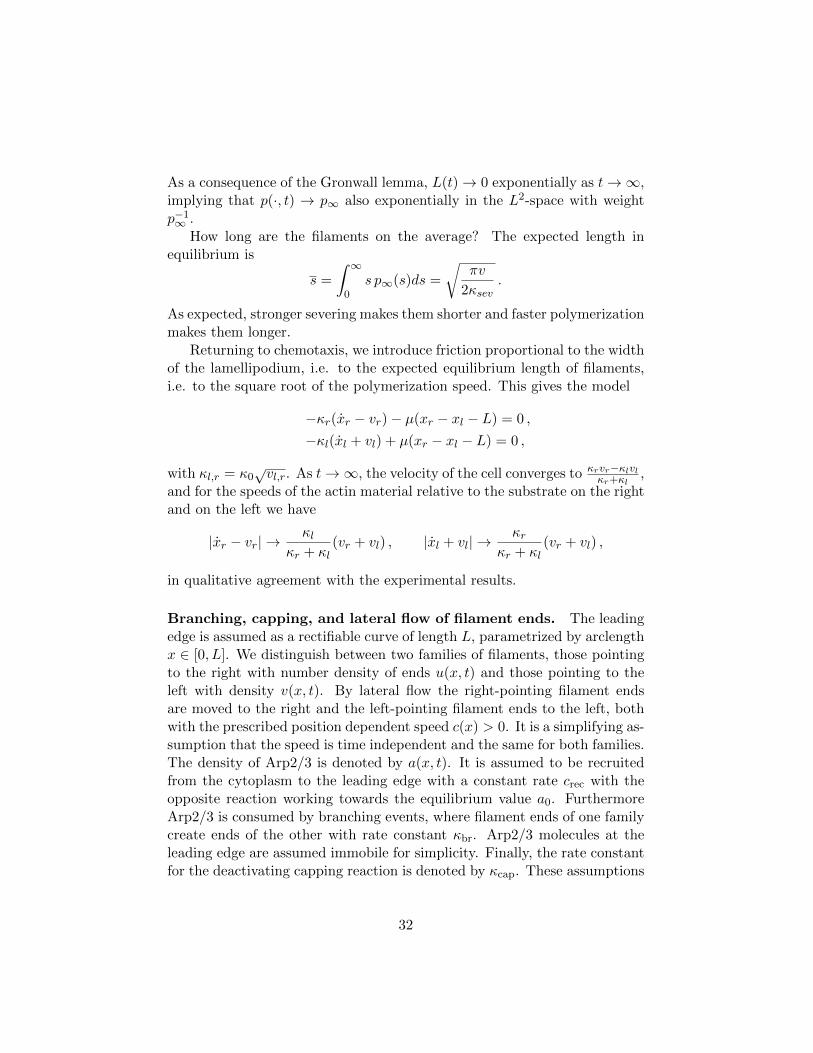
Length distribution of actin filaments. An obvious consequence ofthe model in the previous paragraph is that the speed of the cytoskeletonrelative to the substrate is the same in the front part of the lamellipodiumon the right and in the rear part on the left, i.e. |xr − vr| = |xl + vl|. Thiscontradicts experimental results, see Fig. 4. An explanation is that thehigher polymerization speed in the front part produces longer filaments andtherefore a wider lamellipodium with stronger friction than on the rear side.

This motivates to study the length distribution of actin filaments. Weassume that at the leading edge the barbed ends of the filaments are at-tached and polymerize with a given speed v. Among several possible typesof depolymerization mechanisms, we describe severing, which means that

28

Figure 4: Measurement of the velocity relative to the substrate of the cy-toskeleton of a fish keratocyte moving upwards.

filaments can be cut at any position. The cut-off piece is assumed not toplay a role any more and is therefore disregarded. Actually it is expectedto be completely decomposed very fast. The severing process is modeledas stochastic with randomly chosen severing times and randomly chosensevering positions. This is an example for a compound Poisson process.

Compound Poisson processes: A compound Poisson process is a stochasticprocess, where random jumps in a state space occur at random times, where thejump times are Poisson distributed and the distribution of the jumps is prescribed.We only present the evolution of the probability density, and we start with a finitestate space, say 1, . . . , n. The probability of the state i at time t is denoted bypi(t), i = 1, . . . , n. Thus, pi(t) ≥ 0 and

∑ni=1 pi(t) = 1 for all t. For the evolution

of the probability distribution we postulate the master equation

dpidt

=

n∑j=1

Wj→i pj − λipi , with λi =

n∑j=1

Wi→j , i = 1, . . . , n ,

and with given Wi→j ≥ 0, i, j = 1, . . . , n (assuming Wi→i = 0). The interpretationis that λi is the Poisson parameter for jumping away from state i, and that, in casea jump away from state i occurs, ki→j := Wi→j/λi is the probability to jump fromi to j. Note that (ki→j)j=1,...,n is a probability distribution on the state space.

The first order chemical reaction networks considered in Section 2 are an exam-ple. In the system (6) the unknown ci(t) could also be interpreted as the probabilityof an individual molecule, changing between the species by the chemical reactions,to belong to the species i at time t.

More generally, let the state space (S, dµ) be a general measure space andp(s, t), s ∈ S, t ∈ IR, the probability density for a compound Poisson process. Then

29

the master equation is given by

∂tp(s, t) =

∫S

W (s′ → s)p(s′, t)dµ(s′)− λ(s)p(s, t) ,

with λ(s) =

∫S

W (s→ s′)dµ(s′) .

For actin filament severing, we assume that the Poisson parameter for afilament to get cut is proportional to its length s ∈ S = (0,∞) (S equippedwith the Lebesgue measure), i.e. λ(s) = κsevs, κsev > 0. Cutting a filamentmeans a jump to a smaller length s′, where we assume a uniform distributionof the cutting position s′ on [0, s], i.e. k(s → s′) = H(s − s′)/s with theHeavyside function H. This gives W (s→ s′) = κsevH(s−s′) and the masterequation

∂tp = K(p) := κsev

(∫ ∞s

p′ds′ − sp),

where the abbreviation p′ means evaluation at s′. With this model filamentswould get shorter and shorter and the probability distribution would con-centrate more and more at s = 0. This effect is balanced by polymerization,which we assume to happen with fixed given speed v, leading to the completemodel

∂tp+ v∂sp = K(p) .

Because of v > 0, a boundary condition at s = 0 is needed. We assume thatno new filaments are nucleated, leading to

p(0, t) = 0 , for all t .

At first glance, this partial integro-differential equation looks rather compli-cated. It helps to rewrite it in conservation form:

∂tp+ ∂s

(vp− κsevs

∫ ∞s

p′ds′)

= 0 .

We look for an equilibrium distribution p∞(s) with vanishing flux:

vp∞κsevs

=

∫ ∞s

p′∞ds′ .

Taking the derivative of this equation with respect to s leads to a first orderlinear ordinary differential equation for p∞, which can be solved explicitly:

p∞(s) =κsevs

vexp

(−κsevs

2

2v

),

30

where the integration constant has been chosen such that p∞ is a proba-bility distribution. Analogously to Section 2, we show the stability of theequilibrium by using the Lyapunov function

L(t) =1

2

∫ ∞0

p∞u2ds , with u(s, t) =

p(s, t)− p∞(s)

p∞(s),

satisfying

dL

dt=

∫ ∞0

u(K(p)− v∂sp)ds .

We compute∫ ∞0

u∂sp ds =

∫ ∞0

u∂s(p∞u+ p∞)ds

=

∫ ∞0

(u2 + u)∂sp∞ ds+

∫ ∞0

p∞∂s

(u2

2

)ds

=

∫ ∞0

(u2

2+ u

)∂sp∞ ds ,

which gives

dL

dt=

∫ ∞0

uK(p)ds−∫ ∞

0

(u2

2+ u

)K(p∞)ds

=

∫ ∞0

uK(p∞u)ds−∫ ∞

0

u2

2K(p∞)ds

= κsev

∫ ∞0

∫ ∞0

[H(s′ → s)p′∞

(u′u− u2

2

)−H(s→ s′)p∞

u2

2

]ds′ds .

Interchanging s and s′ in the second part leads to

dL

dt= −κsev

2

∫ ∞0

∫ ∞0

H(s′ → s)p′∞(u− u′)2ds′ds ,

showing already that L is a Lyapunov function. Symmetrization and thefact that max p∞ =

√κsev/(ev) imply

dL

dt= −κsev

4

∫ ∞0

∫ ∞0

(H(s′ → s)p′∞ +H(s→ s′)p∞

)(u− u′)2ds′ds

≤ −√κsevev

4

∫ ∞0

∫ ∞0

(H(s′ → s) +H(s→ s′)

)p′∞p∞(u− u′)2ds′ds

= −√κsevev L .

31

As a consequence of the Gronwall lemma, L(t)→ 0 exponentially as t→∞,implying that p(·, t) → p∞ also exponentially in the L2-space with weightp−1∞ .

How long are the filaments on the average? The expected length inequilibrium is

s =

∫ ∞0

s p∞(s)ds =

√πv

2κsev.

As expected, stronger severing makes them shorter and faster polymerizationmakes them longer.

Returning to chemotaxis, we introduce friction proportional to the widthof the lamellipodium, i.e. to the expected equilibrium length of filaments,i.e. to the square root of the polymerization speed. This gives the model

−κr(xr − vr)− µ(xr − xl − L) = 0 ,

−κl(xl + vl) + µ(xr − xl − L) = 0 ,

with κl,r = κ0√vl,r. As t→∞, the velocity of the cell converges to κrvr−κlvl

κr+κl,

and for the speeds of the actin material relative to the substrate on the rightand on the left we have

|xr − vr| →κl

κr + κl(vr + vl) , |xl + vl| →

κrκr + κl

(vr + vl) ,

in qualitative agreement with the experimental results.

Branching, capping, and lateral flow of filament ends. The leadingedge is assumed as a rectifiable curve of length L, parametrized by arclengthx ∈ [0, L]. We distinguish between two families of filaments, those pointingto the right with number density of ends u(x, t) and those pointing to theleft with density v(x, t). By lateral flow the right-pointing filament endsare moved to the right and the left-pointing filament ends to the left, bothwith the prescribed position dependent speed c(x) > 0. It is a simplifying as-sumption that the speed is time independent and the same for both families.The density of Arp2/3 is denoted by a(x, t). It is assumed to be recruitedfrom the cytoplasm to the leading edge with a constant rate crec with theopposite reaction working towards the equilibrium value a0. FurthermoreArp2/3 is consumed by branching events, where filament ends of one familycreate ends of the other with rate constant κbr. Arp2/3 molecules at theleading edge are assumed immobile for simplicity. Finally, the rate constantfor the deactivating capping reaction is denoted by κcap. These assumptions

32

lead to the system

∂tu+ ∂x(c(x)u) = κbra

a0v − κcapu ,

∂tv − ∂x(c(x)v) = κbra

a0u− κcapv ,

∂ta = crec

(1− a

a0

)− κbr

a

a0(u+ v) .

We introduce the scaling

x→ xL, t→ t

κcap, c(x)→ Lκcapc(x), (u, v)→

(ucrec

κbr, vcrec

κbr

), a→ a0a,

and the dimensionless parameters

α :=κbr

κcap, ε =

κcapa0

crec,

where α, the ratio between the branching and the capping rates, is assumedof moderate size, whereas ε, the ratio between the characteristic time forArp2/3 and that of the capping and branching processes will be assumedas small. Whereas the first assumption is justified and actually necessary,as our analysis will show, the smallness of ε has, to the knowledge of theauthor, not been verified experimentally. The nondimensionalized systemhas the form

∂tu+ ∂x(c(x)u) = αav − u ,∂tv − ∂x(c(x)v) = αau− v ,

ε∂ta = 1− a(1 + u+ v) .

The last step in the model derivation is to pass to the quasistationary limitε→ 0 in the equation for a, which is analogous to the derivation of Michaelis-Menten kinetics. Elimination of a from the resulting system gives

∂tu+ ∂x (c(x)u) =α v

1 + u+ v− u ,

∂tv − ∂x (c(x)v) =αu

1 + u+ v− v , (37)

for x ∈ [0, 1]. Two types of boundary conditions are biologically relevant.In the case of a ring-shaped lamellipodium around the whole cell we assumeperiodic boundary conditions. On the other hand, if we consider only alamellipodium at the front, it is reasonable to assume that no left-moving

33

filaments enter from the right and vice versa. These considerations allow tocomplement (37) with one of the following sets of boundary conditions:

(DBC) u(0, t) = 0, v(1, t) = 0, for t > 0 , (38)

(PBC) u(0, t) = u(1, t), v(0, t) = v(1, t), for t > 0. (39)

For (PBC) we implicitly assume that also the lateral flow speed c(x) is pe-riodic. To complete the definition of the problem, we pose initial conditions

u(x, 0) = u0(x) , v(x, 0) = v0(x) , for x ∈ [0, 1] , (40)

with given u0(x), v0(x), which are assumed to be non-negative and to satisfythe boundary conditions.

It turns out that the value of the parameter α is critical for the dynamicbehavior. It can be shown that for α < 1 the filament network dies outexponentially, whereas for α bigger than a bifurcation value α0 ≥ 1, existenceand stability of a nontrivial steady state can be expected. For details on theanalysis see [6].

References

[1] G. Bernot, J.-P. Comet, A. Richard, M. Chaves, J.-L. Gouze, F. Dayan,Modeling and analysis of gene regulatory networks, in Modeling inComputational Biology and Biomedicine, A Multidisciplinary Endeavor(eds. F. Cazals and P. Kornprobst). pp. 47-80, Springer, 2013.

[2] E. Bianconi et al., An estimation of the number of cells in the humanbody, Ann. Hum. Biol. 40(6) (2013), pp. 463–471.

[3] L.C. Evans, Partial Differential Equations, Graduate Studies in Math-ematics 19, AMS, Providence, 1998.

[4] K. Fellner, W. Prager, B.Q. Tang, The entropy method for reaction-diffusion systems without detailed balance: first order chemical reactionnetworks, arXiv: 1504.08221

[5] A.F. Filippov, Differential equations with discontinuous right hand side,AMS Transl. 42 (1962), pp. 199–231.

[6] A. Manhart, C. Schmeiser, Existence of and decay to equilib-rium of the filament end density along the leading edge ofthe lamellipodium, J. Math. Biol. (2016), online first (pdf onhttp://homepage.univie.ac.at/christian.schmeiser/publications1.htm).

34

[7] L. Michaelis, M. L. Menten, Die Kinetik der Invertinwirkung, Biochem.Z. 49 (1913), pp. 333-369.

[8] V. Milisic, D. Oelz, J. Math. Pures Appl. 96 (2011), pp. 484–501.

[9] K. Parmar, K.B. Blyuss, Y.N. Kyrychko, S.J. Hogan, Time-delayedmodels of gene regulatory networks, Comp. and Math. Meth. inMedicine 2015 (2015), Article ID 347273.

[10] Q.-C. Pham, A variation of Gronwall′s lemma, arXiv: 0704.0922v3.

[11] T. Scheper, D. Klinkenberg, C. Pennartz, J. v. Pelt, A mathematicalmodel for the intracellular circadian rhythm generator, J. of Neurosci.19 (1999), pp. 40–47.

35