Embed Size (px)
Citation preview
Mathematical challenges and approaches in EMtomographic reconstruction
Ozan [email protected]
Sidec AB
May 14, 2008Lorenz Center: New algorithms in macromolecular crystallography and
electron microscopy
Outline
1 The model for image formation and the reconstruction problem in ET
2 Reconstruction methods in ET
3 Classical regularisation theory
4 Statistical regularisation theory

The model from image formation
Assume perfect coherent imaging, so the scattering properties of thespecimen are given by the electrostatic potential and theelectron-specimen interaction is modelled by the scalar Schrodingerequation.
The high energy approximation allows us to replace the Schrodingerequation with the projection operator P (X-ray transform).
TEM optics and detector are both modelled as convolution operators.
Inelastic scattering and incoherent illumination introduces partialincoherence, so the basic assumption of perfect coherent imagingmust be relaxed.The intensity at a point is given as the projection of the potentialconvolved with the optics PSF. A tiltseries g is a sample of a randomvariable G = C + E where
I C is a correlated Poisson random variable with the intensity as itsmean (correlation is introduced by the detector PSF).
I E is the noise introduced by detector.
The reconstruction problem in ETFormulation and difficulties
The reconstruction problem in ET
Recover the scattering potential f from the measured tiltseries g which isa single sample of the stochastic variable G modelling the data.
Any attempt at solving the reconstruction problem in ET has to deal withthe following:
The dose problem: Leads to data with significant amount of noise.
Limited angle problem: Leads to severe instability.
Local tomography: Leads to non-uniqueness.
Therefore
the reconstruction problem in ET is severely unstable (ill-posed), and
a reliable reconstruction method must include some kind ofstabilisation (regularisation).
Regularisation methods applied to ETFurther difficulties
Besides the severe ill-posedness, there are two additional peculiarities inET that makes it difficult to apply an off-the shelf regularisation method.
No reliable a priori estimate of data error. This makes it difficult to apriori determine the degree of stabilisation (i.e. the regularisationparameter(s)).In ET we are dealing with a multi-component reconstruction problem,i.e. there are parameters which are additional unknowns that needs tobe reconstructed alongside the scattering potential:Independent of specimen, dependent on tilt: TEM imaging
parameters, e.g. incoming dose and defocus.Dependent of specimen: Parameters used for describing the
scattering potential outside the region of interest andthe (tilt dependent) phase contrast ratio.
Note: Parameters independent of the specimen and tilt, e.g. detectorrelated parameters, can be determined beforehand.

Reconstruction methods in ETOverview of approaches
T denotes the forward operator which is defined as the expected value ofthe stochastic variable G modelling the data (i.e. the measured tiltseries gis a sample of G ).
Analytic methods: Based on discretising the inverse of T . Regularisationis obtained by constructing an approximate inverserecovering only those features that can be stably retrieved.Example: Filter backprojection (FBP) with de-noising,Λ-tomography for the recovery of boundaries (edges).
Iterative methods: Discretise T (f ) = g and solve by an iterative method.Regularisation is obtained by early stopping.Example: Conjugate gradient methods, ART, SIRT, Newtonmethods.
Variational regularisation methods
Classical regularisation theoryAbstract reconstruction problem
The abstract reconstruction problem
Assume that g ∈H is related to f ∈X by the model T (f ) = g . Recoverf ∈X from g ∈H .
In the above:
H is the data space, i.e. the set of all possible data, and g ∈H isthe measured data. We will henceforth assume that H ' Rm wherem is the number of data points.
X is the reconstruction space, i.e. the set of feasible solutions, andf ∈X represents the unknown object of primary interest that is tobe recovered. In ET, X are functions in L 1
⋂L 2 with positive real
and imaginary parts.
T : X →H is the forward operator which is the mathematical modelfor the experiment relating the unknown f to the measured data g .

Classical regularisation theoryConcept of ill-posedness
An important problem that arises when trying to solve
T (f ) = g (1)
is that there might be no solutions at all (non-existence).Existence is commonly enforced by considering least squares solutions to(1), i.e. (1) is replaced with
minf ∈X
∥∥T (f )− g∥∥
H
for a suitable choice of distance measure∥∥ · ∥∥
Hin data space H .
Two serious problems remain:
Infinitely many least squares solutions (non-uniqueness).
The least squares solution does not depend continuously on the datag (instability).
(1) is ill-posed if any of these issues occur.

Classical regularisation theoryBasic principle of regularisation
Special care must be taken when dealing with ill-posed reconstructionproblems. The reconstruction method must involve some stabilisation, i.e.it must act as a regularisation method.
The main idea
The main idea underlying a regularisation method is to replace the originalill-posed reconstruction problem by a well-posed reconstruction problem(i.e. it has a unique solution that depends continuously on the data) thatis convergent as the data error goes to zero.
Well-posedness: Guarantees stability
Convergence: The reconstructions obtained converge to a least squaressolution when the data error approaches zero and theparameters in the reconstruction method (regularisationparameters) are chosen appropriately.
Classical regularisation theoryMathematical analysis of regularisation methods
Besides convergence, the performance of a regularisation method dependson
the accuracy of the forward operator T modelling the experiment,
how well it can account for the actual stochasticity of the data g ,
how well it captures a priori knowledge about the solution f , and
on finding the right compromise between accuracy and stability byselecting the regularisation parameter(s).
Analytic methods: Filtered backprojection methodBasic assumptions
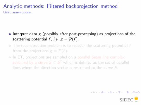
Interpret data g (possibly after post-processing) as projections of thescattering potential f , i.e. g = P(f ).
The reconstruction problem is to recover the scattering potential ffrom the projections g = P(f ).
In ET, projections are sampled on a parallel beam line complexspecified by a curve S ⊂ S2 which is defined as the set of parallellines where the direction vector is restricted to the curve S .

Analytic methods: Filtered backprojection methodBasic assumptions
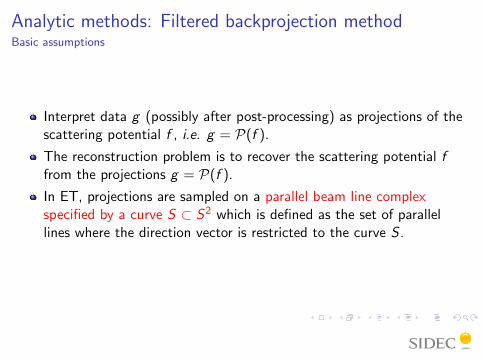
Interpret data g (possibly after post-processing) as projections of thescattering potential f , i.e. g = P(f ).
The reconstruction problem is to recover the scattering potential ffrom the projections g = P(f ).
In ET, projections are sampled on a parallel beam line complexspecified by a curve S ⊂ S2 which is defined as the set of parallellines where the direction vector is restricted to the curve S .
Analytic methods: Filtered backprojection methodBasic assumptions
Interpret data g (possibly after post-processing) as projections of thescattering potential f , i.e. g = P(f ).
The reconstruction problem is to recover the scattering potential ffrom the projections g = P(f ).
In ET, projections are sampled on a parallel beam line complexspecified by a curve S ⊂ S2 which is defined as the set of parallellines where the direction vector is restricted to the curve S .

Analytic methods: Filtered backprojection methodReconstruction scheme
Reconstruction operator: For a function g defined on a parallel beam linecomplex specified by the curve S ⊂ S2, define
LFBP(g) := P∗S(h ~ω⊥
g)
where
h is the reconstruction filter
P∗S is the back-projection restricted to the curve of directions S :
P∗S(g)(x) :=
∫S
g(ω, x− (x ·ω)ω
)dω where x ∈ R3.
Note: The pair (ω, x), where ω ∈ S is the direction of the line and x ∈ω⊥ as a point on the line, uniquely determines a line and thereby acts ascoordinates on the parallel beam line complex.

Analytic methods: Filtered backprojection methodReconstruction scheme
Reconstruction operator: For a function g defined on a parallel beam linecomplex specified by the curve S ⊂ S2, define
LFBP(g) := P∗S(h ~ω⊥
g)
where
h is the reconstruction filter
P∗S is the back-projection restricted to the curve of directions S :
P∗S(g)(x) :=
∫S
g(ω, x− (x ·ω)ω
)dω where x ∈ R3.
Rationale: If g = P(f ), then one can show that
LFBP(g) = H ∗ f where H := P∗S(h).
Exact FBP: Choose h such that H = δ.

Analytic methods: Filtered backprojection methodProblems
Limited data: Due to the limited angle problems in ET, S does not fulfilOrlov’s condition and the reconstruction problem is severelyill-posed. Local tomography introduces non-uniquness evenfor noise free continuos data.
Difficult to regularise: If data g is not consistent, then discretised exactFBP gives a least squares solution. Thus, one mustregularise. Crowther’s regularisation criterion based onband-limiting the filter doesn’t work well with very noisydata.
Difficult to account for data stochasticity: Difficult (if not impossible) todevise schemes for selecting the filter h that takes intoaccount the specific stochasticity of the data.
Simplified model for imaging: Data is assumed to be samples of aprojection, so optics and detector PSF’s must either bedeconvolved or ignored.
Analytic methods: Λ-tomographyBasic assumptions and principle
In ET one has limited angle local tomography data. Therefore, one cannotexactly reconstruct the scattering potential of the specimen even in caseswhen one assumes to have a continuum of exact data!
Solution proposed by Λ-tomography
Reconstruct only some information about the specimen that can be stablyretrieved, in our case the singularities of the scattering potential, i.e. theboundaries of the molecules in the specimen.
Λ-tomography is based on the same assumptions as FBP.
Reference(s)
Local Tomography in Electron MicroscopyQuinto E T and Oktem OSIAM Journal on Applied Mathematics 68(5), pp. 1282–1303, 2008

Analytic methods: Λ-tomographyReconstruction scheme
Reconstruction operator: For a function g defined on a parallel beam linecomplex specified by the curve S ⊂ S2, define
LΛ(g) := P∗SD2Sg
where D2S is a second order differentiation along the tangential direction to
the curve S , i.e.
D2Sg(ω, x
):=
d2
ds2g(ω, x + sσ
)∣∣∣s=0
with σ denoting the unit tangent to S at ω ∈ S .Rationale: If g = P(f ), then using microlocal analysis one can show thatthe visible singularities of f coincide with those of LΛ(g). Moreover, thevisible singularities can be precisely described and the recovery is onlymildly ill-posed even in the case of missing data.
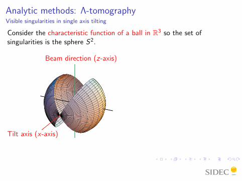
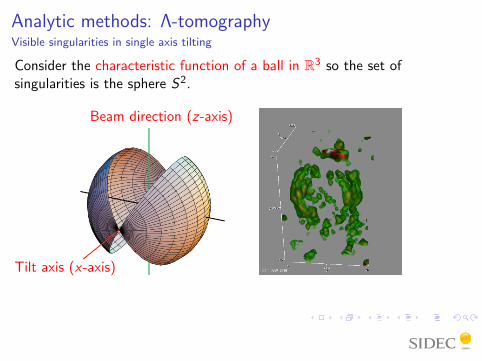
Analytic methods: Λ-tomographyVisible singularities in single axis tilting
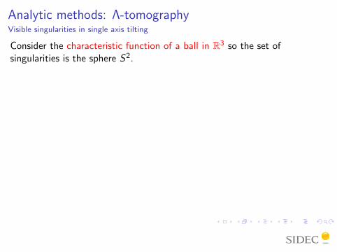
Consider the characteristic function of a ball in R3 so the set ofsingularities is the sphere S2.
Tilt axis (x-axis)
Beam direction (z-axis)
Analytic methods: Λ-tomographyVisible singularities in single axis tilting
Consider the characteristic function of a ball in R3 so the set ofsingularities is the sphere S2.
Tilt axis (x-axis)
Beam direction (z-axis)
Analytic methods: Λ-tomographyVisible singularities in single axis tilting
Consider the characteristic function of a ball in R3 so the set ofsingularities is the sphere S2.
Tilt axis (x-axis)
Beam direction (z-axis)

Analytic methods: FBP vs. Λ-tomographyThe PSF’s of Λ-tomography and FBP in single axis tilting
FBP point spread function Λ-tomograhy point spreadfunction

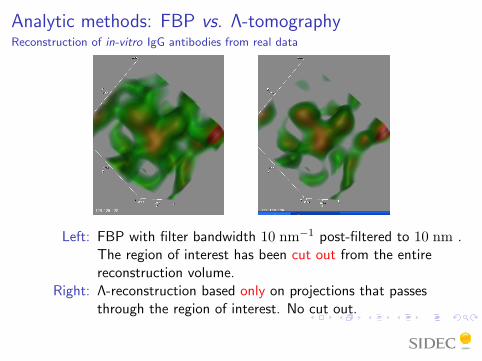
Analytic methods: FBP vs. Λ-tomographyReconstruction of in-vitro IgG antibodies from real data
Specimen: In-vitro specimen with monoclonal IgG antibodies (molecularweight about 150 kDa).
Data: 200 keV TEM single axis tilt data at 1 µm under-focus witha uniform sampling of the tilt angle in [−60◦, 60◦] at 2◦ step.The total dose is 1520 e−/nm2.
Reconstruction: Region of interest is a 50× 50× 50 voxel large with avoxel size of 0.5241 nm.
Analytic methods: FBP vs. Λ-tomographyReconstruction of in-vitro IgG antibodies from real data
Left: FBP with filter bandwidth 10 nm−1 post-filtered to 10 nm .The region of interest has been cut out from the entirereconstruction volume.
Right: Λ-reconstruction based only on projections that passesthrough the region of interest. No cut out.

Analytic methods: FBP vs. Λ-tomographyReconstruction of in-situ tissue sample
Specimen: In-situ specimen from a kidney tissue sample.
Data: 200 kV TEM single axis tilt data at 1 µm under-focus with auniform sampling of the tilt angle in [−60◦, 60◦] at 2◦ step.The total dose is 1520 e−/nm2.
Reconstruction: Region of interest is a 200× 200× 140 voxel large with avoxel size of 0.5241 nm.

Analytic methods: FBP vs. Λ-tomographyReconstruction of in-situ tissue sample
Left: FBP with filter bandwidth 10 nm−1 post-filtered to 3 nm.
Right: Λ-reconstruction post-filtered to 3 nm.

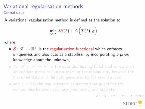
Variational regularisation methodsGeneral setup
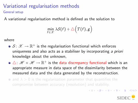
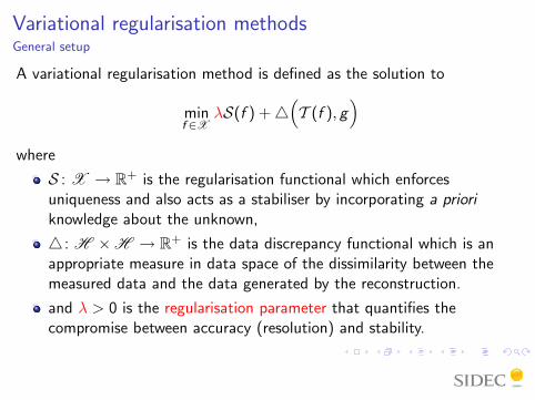
A variational regularisation method is defined as the solution to
minf ∈X
λS(f ) +4(T (f ), g
)
where
S : X → R+ is the regularisation functional which enforcesuniqueness and also acts as a stabiliser by incorporating a prioriknowledge about the unknown,
4 : H ×H → R+ is the data discrepancy functional which is anappropriate measure in data space of the dissimilarity between themeasured data and the data generated by the reconstruction.
and λ > 0 is the regularisation parameter that quantifies thecompromise between accuracy (resolution) and stability.
Variational regularisation methodsGeneral setup
A variational regularisation method is defined as the solution to
minf ∈X
λS(f ) +4(T (f ), g
)where
S : X → R+ is the regularisation functional which enforcesuniqueness and also acts as a stabiliser by incorporating a prioriknowledge about the unknown,
4 : H ×H → R+ is the data discrepancy functional which is anappropriate measure in data space of the dissimilarity between themeasured data and the data generated by the reconstruction.
and λ > 0 is the regularisation parameter that quantifies thecompromise between accuracy (resolution) and stability.

Variational regularisation methodsCommon approaches
Choice of regularisation functional: The choice should be based on a prioriknowledge about the unknowns.
Prior information Regularisation functional
True solution is sparse in the voxel representation (i.e. truesolution behaves like few outstanding features in alow-amplitude background).
S(f ) = ‖f ‖L p =`R
X
˛f (x)
˛p dx´1/p with 0 ≤ p ≤ 1
S(f ) =RX
“f (x) ln
f (x)ρ(x)−f (x)+ρ(x)
”dx with ρ ∈X
Gradient of the true solution is sparse in the voxel represen-tation (i.e. the true solution behaves like a step function).Case with p = 1 is the TV-regularsiation.
S(f ) = ‖∇f ‖L p =`R
X
˛∇f (x)
˛p dx´1/p with 0 ≤
p ≤ 1.
True solution has edges but is smoothly varying away fromedges.
S(f ) =RX
˛∇f (x)
˛p(|∇f (x)|) dx where p : R+ → [0, 2]is monotonically decreasing.
Edges in the true solution along specific directions are bettercharacterised than the remaining edges.
S(f ) =RX φ
`|∇f (x)|
´dx where φ : Rn → R is con-
vex, zero at the origin, and positively 1-homogenous.
True solution is smooth. S(f ) = ‖∇f ‖L 2 =
qRX
˛∇f (x)
˛2 dx
True solution is sparse in some representation {φi}i , i.e. f =Pi αiφi where most αi ≈ 0.
S(f ) =`P
i |αi |p´1/p with 0 ≤ p ≤ 1

Variational regularisation methodsCommon approaches
Choice of data discrepancy functional: The choice should be based on knowl-edge of the probability model for the data stochasticity. Here ‖ · ‖`p denotesthe Euclidian p-norm in H ' Rm.
Model for data stochasticity Data discrepancy functional
Data is contaminated with additive Gaussian noisewith zero mean and covariance matrix Σ.
4`T (f ), g
´= ‖T (f )− g‖
`2
4`T (f ), g
´=q`T (f )− g
´t ·Σ−1 ·`T (f )− g
´Data is Poisson distributed with mean given by ac-tual measurement, i.e. noise is signal dependent.
4`T (f ), g
´=Pm
i=1 gi logT (f )i − T (f )i
The noise in data is impulse noise in which arandom portion of the data points are corrupted,e.g. salt and pepper noise.
4`T (f ), g
´= ‖T (f )− g‖
`0
4`T (f ), g
´= ‖T (f )− g‖
`1
Variational regularisation methodsCommon approaches
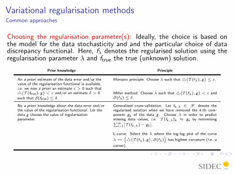
Choosing the regularisation parameter(s): Ideally, the choice is based onthe model for the data stochasticity and and the particular choice of datadiscrepancy functional. Here, fλ denotes the regularised solution using theregularisation parameter λ and ftrue the true (unknown) solution.
Prior knowledge Principle
An a priori estimate of the data error and/or thevalue of the regularisation functional is available,i.e. we now a priori an estimate ε > 0 such that4`T (ftrue), g
´< ε and/or an estimate δ > 0
such that S(ftrue) ≤ δ.
Morozov principle: Choose λ such that 4`T (fλ), g
´≤ ε.
Miller method: Choose λ such that 4`T (fλ), g
´< ε and
S(fλ) ≤ δ.
No a priori knowledge about the data error and/orthe value of the regularisation functional. Let thedata g choose the value of regularisationparameter.
Generalised cross-validation: Let fk,λ ∈ X denote theregularised solution when we have removed the k:th com-ponent gk of the data g . Choose λ in order to predictmissing data values, i.e. T (fk,λ)k ≈ gk by minimisingPm
i=1
˛T (fk,λ)− gk
˛.
L-curve: Select the λ where the log-log plot of the curve
λ 7→“4`T (fλ), g
´,S(fλ)
”has highest curvature (i.e. a
corner).
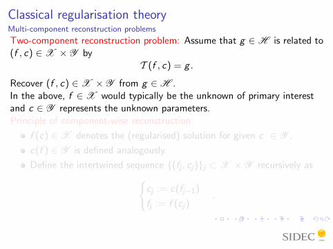
Classical regularisation theoryMulti-component reconstruction problems
Two-component reconstruction problem: Assume that g ∈H is related to(f , c) ∈X × Y by
T (f , c) = g .
Recover (f , c) ∈X × Y from g ∈H .In the above, f ∈X would typically be the unknown of primary interestand c ∈ Y represents the unknown parameters.Principle of component-wise reconstruction:
f (c) ∈X denotes the (regularised) solution for given c ∈ Y .
c(f ) ∈ Y is defined analogously.
Define the intertwined sequence {(fj , cj)}j ⊂X × Y recursively as{cj := c(fj−1)
fj := f (cj).

COMETOverview
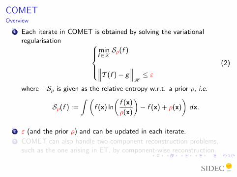
1 Each iterate in COMET is obtained by solving the variationalregularisation
minf ∈XSρ(f )
∥∥∥T (f )− g∥∥∥
H≤ ε
(2)
where −Sρ is given as the relative entropy w.r.t. a prior ρ, i.e.
Sρ(f ) :=
∫ (f (x) ln
(f (x)
ρ(x)
)− f (x) + ρ(x)
)dx.
2 ε (and the prior ρ) and can be updated in each iterate.3 COMET can also handle two-component reconstruction problems,
such as the one arising in ET, by component-wise reconstruction.
COMETOverview
1 Each iterate in COMET is obtained by solving the variationalregularisation
minf ∈XSρ(f )
∥∥∥T (f )− g∥∥∥
H≤ ε
(2)
where −Sρ is given as the relative entropy w.r.t. a prior ρ, i.e.
Sρ(f ) :=
∫ (f (x) ln
(f (x)
ρ(x)
)− f (x) + ρ(x)
)dx.
2 ε (and the prior ρ) and can be updated in each iterate.3 COMET can also handle two-component reconstruction problems,
such as the one arising in ET, by component-wise reconstruction.
COMETThe regularisation parameters
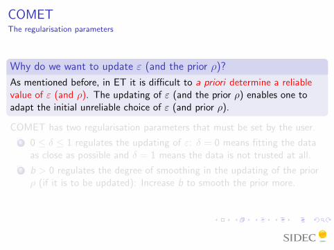
Why do we want to update ε (and the prior ρ)?
As mentioned before, in ET it is difficult to a priori determine a reliablevalue of ε (and ρ). The updating of ε (and the prior ρ) enables one toadapt the initial unreliable choice of ε (and prior ρ).
COMET has two regularisation parameters that must be set by the user.
1 0 ≤ δ ≤ 1 regulates the updating of ε: δ = 0 means fitting the dataas close as possible and δ = 1 means the data is not trusted at all.
2 b > 0 regulates the degree of smoothing in the updating of the priorρ (if it is to be updated): Increase b to smooth the prior more.

COMETThe regularisation parameters
Why do we want to update ε (and the prior ρ)?
As mentioned before, in ET it is difficult to a priori determine a reliablevalue of ε (and ρ). The updating of ε (and the prior ρ) enables one toadapt the initial unreliable choice of ε (and prior ρ).
COMET has two regularisation parameters that must be set by the user.
1 0 ≤ δ ≤ 1 regulates the updating of ε: δ = 0 means fitting the dataas close as possible and δ = 1 means the data is not trusted at all.
2 b > 0 regulates the degree of smoothing in the updating of the priorρ (if it is to be updated): Increase b to smooth the prior more.
COMETThe iterative scheme
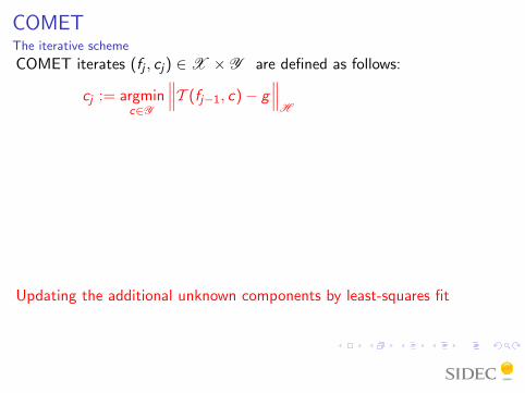
COMET iterates (fj , cj) ∈X × Y are defined as follows:
cj := argminc∈Y
∥∥∥T (fj−1, c)− g∥∥∥
H
ρj :=
{Fb(fj−1) if prior is to be updated,
ρ if prior is not updated,
εj := εmin(g , cj) + δ
(∥∥∥T (ρj , cj)− g∥∥∥
H− εmin(g , cj)
)
fj :=
argminf ∈X
Sρj (f )∥∥∥T (f , cj)− g∥∥∥
H≤ εj .
Updating the additional unknown components by least-squares fit
εmin(g , c) := inff ∈X
∥∥∥T (f , c)− g∥∥∥
H
COMETThe iterative scheme
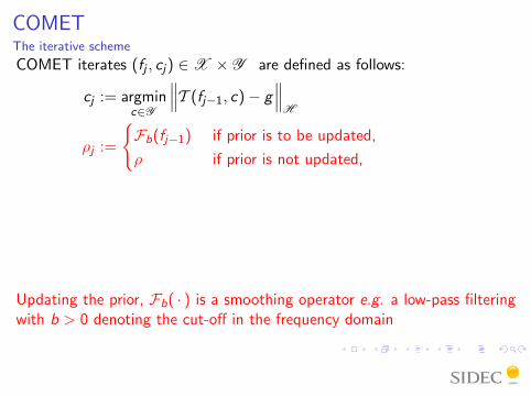
COMET iterates (fj , cj) ∈X × Y are defined as follows:
cj := argminc∈Y
∥∥∥T (fj−1, c)− g∥∥∥
H
ρj :=
{Fb(fj−1) if prior is to be updated,
ρ if prior is not updated,
εj := εmin(g , cj) + δ
(∥∥∥T (ρj , cj)− g∥∥∥
H− εmin(g , cj)
)
fj :=
argminf ∈X
Sρj (f )∥∥∥T (f , cj)− g∥∥∥
H≤ εj .
Updating the prior, Fb( · ) is a smoothing operator e.g. a low-pass filteringwith b > 0 denoting the cut-off in the frequency domain
εmin(g , c) := inff ∈X
∥∥∥T (f , c)− g∥∥∥
H

COMETThe iterative scheme
COMET iterates (fj , cj) ∈X × Y are defined as follows:
cj := argminc∈Y
∥∥∥T (fj−1, c)− g∥∥∥
H
ρj :=
{Fb(fj−1) if prior is to be updated,
ρ if prior is not updated,
εj := εmin(g , cj) + δ
(∥∥∥T (ρj , cj)− g∥∥∥
H− εmin(g , cj)
)
fj :=
argminf ∈X
Sρj (f )∥∥∥T (f , cj)− g∥∥∥
H≤ εj .
Updating the estimate of the data error,
εmin(g , c) := inff ∈X
∥∥∥T (f , c)− g∥∥∥
H

COMETThe iterative scheme
COMET iterates (fj , cj) ∈X × Y are defined as follows:
cj := argminc∈Y
∥∥∥T (fj−1, c)− g∥∥∥
H
ρj :=
{Fb(fj−1) if prior is to be updated,
ρ if prior is not updated,
εj := εmin(g , cj) + δ
(∥∥∥T (ρj , cj)− g∥∥∥
H− εmin(g , cj)
)
fj :=
argminf ∈X
Sρj (f )∥∥∥T (f , cj)− g∥∥∥
H≤ εj .
Updating the object that is of primary interest by entropy regularisation
εmin(g , c) := inff ∈X
∥∥∥T (f , c)− g∥∥∥
H
COMETSelecting the regularisation parameters
Setting the regularisation parameters
By empirical experience! For data with good signal-to-noise ratio (typicallyin-situ data), δ ≈ 0.5 and b ≈ 6 nm−1. For data with poor signal-to-noiseratio (typically in-vitro data), δ ≈ 0.8 and b ≈ 10 nm−1.
Ideally, the regularisation parameters δ and b should be set usingknowledge about the stochasticity of the data and an estimate of thedata error.
COMETReferences
Reference(s)
Maximum-entropy three-dimensional reconstruction with deconvolution of thecontrast transfer function: a test application with AdenovirusSkoglund U, Ofverstedt, L-G, Burnett R M and Bricogne G.Journal of Structural Biology 117, 173–88, 1996.First publication describing usage of entropy regularisation in ET. Does not include a
description of the updating of ε and ρ, since at that time those parameters where
constant and assumed to be known a priori.
A component-wise iterated relative entropy regularisation method with updatedprior and regularisation parameterRullgard H, Oktem O and Skoglund U.Inverse Problems 23, 2121–39, 2007.The formal mathematical analysis and description of COMET.

`1-TV regularisation
In `1-regularisation the reconstruction problem is defined by solving
minf ∈XSλ(f ) +
∥∥∥T (f )− g∥∥∥
H
where the regularisation functional Sλ can be defined as
Sλ(f ) := λ1
∥∥f ∥∥L 1 + λ2
∥∥∇f∥∥
L 1
for λ := (λ1, λ2) which is the regularisation parameter for the method.In the above expression,
∥∥ · ∥∥L 1 denotes the L 1-norm, i.e.
∥∥f ∥∥L 1 :=
∫ ∣∣f (x)∣∣ dx and
∥∥∇f∥∥
L 1 :=
∫ ∣∣∇f (x)∣∣ dx
and second term to the right is often referred to as the total variation of f .

`1-TV regularisationSpecific properties
For efficient removal of background noise, the regularisationparameter(s) λ should be chosen so that for a small selection of “testfunctions” htest, e.g. characteristic functions of balls,
2 <Sλ(htest)
σ(htest)< 5 where σ(htest) := Variance
[⟨T (htest),E
⟩H
]1/2
holds. In the above, E is the random variable representing the noisecomponent of the data.
In ET, σ(htest) can be reliably estimated directly from the tilt series.
Finally, for a given choice of λ, one can also estimate the size offeatures that can be recovered.

`1-TV regularisationReferences
Reference(s)
A new principle for choosing regularization parameter in certain inverse problemsRullgard HPre-print available from arXiv (citation code arXiv:0803.3713v1), 2008A parameter choice rule (i.e. method for choosing the regularisation parameter) is
developed for total variation regularisation of reconstruction problems with high levels of
noise in the data. The parameter choice rule is the applied to then reconstruction
problem in electron tomography.

Tests on data

Comparison of various methodsReconstruction of in-vitro RNA polymerase II molecules from simulated data
Specimen: In-vitro specimen with one RNA polymerase II molecule(with a “diameter” of about 13 nm) in a 50 nm thick slab.
Data: Simulated 200 kV TEM single axis tilt data at 24900×magnification with 1 µm under-focus. Uniform sampling ofthe tilt angle in [−60◦, 60◦] at 1◦ step. The total dose is2000 e−/nm2.
Reconstruction: Region of interest is a 200× 200× 200 voxel large with avoxel size of 0.5622 nm.

Comparison of various methodsSlice through reconstruction
Phantom
100 Å
FBP
100 Å
SIRT
100 Å
Size of scale-bar is10 nm.
COMET
100 Å
`1-TV regularisation
100 Å
Statistical reconstruction methodsMain principle
The philosophy is to recast the inverse problem in the form of statisticalquest for information:
Classical reconstruction methods: Reconstructs a single estimate of theunknowns and seeks to answer the question:
What is the value of the unknowns?
Statistical reconstruction methods: Reconstructs the probabilitydistribution of the unknowns and seeks to answer thequestion:
What is our information about the unknowns?

Statistical reconstruction methodsCommon approaches
Maximum Likelihood
Minimum Inaccuracy
Probability Distribution Matching
Minimising measures of information content, e.g. Maximum Entropymethods
Bayesian inference
Bayesian inferenceReformulation of the reconstruction problem
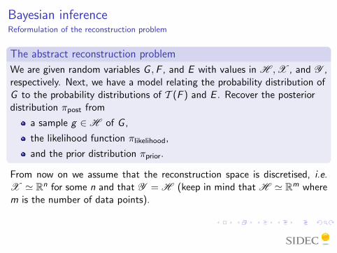
The abstract reconstruction problem
We are given random variables G ,F , and E with values in H ,X , and Y ,respectively. Next, we have a model relating the probability distribution ofG to the probability distributions of T (F ) and E . Recover the posteriordistribution πpost from
a sample g ∈H of G ,
the likelihood function πlikelihood,
and the prior distribution πprior.
G is the random variable with values in data space H modelling themeasured data g ∈H .

Bayesian inferenceReformulation of the reconstruction problem
The abstract reconstruction problem
We are given random variables G ,F , and E with values in H ,X , and Y ,respectively. Next, we have a model relating the probability distribution ofG to the probability distributions of T (F ) and E . Recover the posteriordistribution πpost from
a sample g ∈H of G ,
the likelihood function πlikelihood,
and the prior distribution πprior.
F is the random variable with values in reconstruction space Xmodelling all possible solutions.
Bayesian inferenceReformulation of the reconstruction problem
The abstract reconstruction problem
We are given random variables G ,F , and E with values in H ,X , and Y ,respectively. Next, we have a model relating the probability distribution ofG to the probability distributions of T (F ) and E . Recover the posteriordistribution πpost from
a sample g ∈H of G ,
the likelihood function πlikelihood,
and the prior distribution πprior.
E is the random variable with values in Y modelling additional noisecomponents in the data that are independent of F , typically additiveor multiplicative noise. Often, Y = H .
Bayesian inferenceReformulation of the reconstruction problem
The abstract reconstruction problem
We are given random variables G ,F , and E with values in H ,X , and Y ,respectively. Next, we have a model relating the probability distribution ofG to the probability distributions of T (F ) and E . Recover the posteriordistribution πpost from
a sample g ∈H of G ,
the likelihood function πlikelihood,
and the prior distribution πprior.
Model: Typical examples are G = T (F ) + E or G = C + E where theprobability distribution of C depends on T (F ). Here, T : X →Hdenotes the forward operator.

Bayesian inferenceReformulation of the reconstruction problem
The abstract reconstruction problem
We are given random variables G ,F , and E with values in H ,X , and Y ,respectively. Next, we have a model relating the probability distribution ofG to the probability distributions of T (F ) and E . Recover the posteriordistribution πpost from
a sample g ∈H of G ,
the likelihood function πlikelihood,
and the prior distribution πprior.
Posterior distribution: πpost(f ) := π(f |G = g) is the conditionalprobability distribution of F given G and describes all possiblesolutions and their probabilities.
Bayesian inferenceReformulation of the reconstruction problem
The abstract reconstruction problem
We are given random variables G ,F , and E with values in H ,X , and Y ,respectively. Next, we have a model relating the probability distribution ofG to the probability distributions of T (F ) and E . Recover the posteriordistribution πpost from
a sample g ∈H of G ,
the likelihood function πlikelihood,
and the prior distribution πprior.
Likelihood function: πlikelihood(g) := π(g |F = f ) is the conditionalprobability distribution of G given F that models the stochasticity ofthe data.

Bayesian inferenceReformulation of the reconstruction problem
The abstract reconstruction problem
We are given random variables G ,F , and E with values in H ,X , and Y ,respectively. Next, we have a model relating the probability distribution ofG to the probability distributions of T (F ) and E . Recover the posteriordistribution πpost from
a sample g ∈H of G ,
the likelihood function πlikelihood,
and the prior distribution πprior.
Prior distribution: f 7→ πprior(f ) is the probability distribution of Frepresenting the a priori knowledge we have about the solution to thereconstruction problem.
Bayesian inferenceReformulation of the reconstruction problem
The abstract reconstruction problem
We are given random variables G ,F , and E with values in H ,X , and Y ,respectively. Next, we have a model relating the probability distribution ofG to the probability distributions of T (F ) and E . Recover the posteriordistribution πpost from
a sample g ∈H of G ,
the likelihood function πlikelihood,
and the prior distribution πprior.
From now on we assume that the reconstruction space is discretised, i.e.X ' Rn for some n and that Y = H (keep in mind that H ' Rm wherem is the number of data points).

Bayesian inferenceInverse Problems and Bayes’ Formula
Bayes’ Formula
Assume that for the given measured data g ∈H , the marginaldistribution of G at g is positive, i.e. πG (g) > 0. Then
πpost(f ) =πprior(f )πlikelihood(g)
πG (g).
Note: The marginal distribution πG plays the role of a norming constantand is usually of little importance. If πG (g) = 0, then we have measurementdata g that have zero probability, so the underlying models are not consistentwith the reality.

Bayesian inferenceInverse Problems and Bayes’ Formula
Bayes’ Formula
Assume that for the given measured data g ∈H , the marginaldistribution of G at g is positive, i.e. πG (g) > 0. Then
πpost(f ) =πprior(f )πlikelihood(g)
πG (g).
Solving an inverse problem may therefore be broken into three subtasks:
1 Construction of likelihood function
2 Construction of prior
3 Construction of estimators that allow us to explore the posteriorprobability distribution f 7→ πpost(f ).
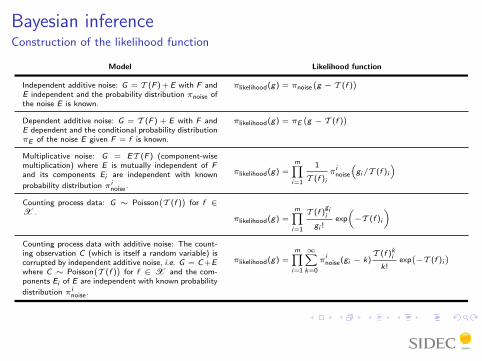
Bayesian inferenceConstruction of the likelihood function
Model Likelihood function
Independent additive noise: G = T (F ) + E with F andE independent and the probability distribution πnoise ofthe noise E is known.
πlikelihood(g) = πnoise`g − T (f )
´
Dependent additive noise: G = T (F ) + E with F andE dependent and the conditional probability distributionπE of the noise E given F = f is known.
πlikelihood(g) = πE`g − T (f )
´
Multiplicative noise: G = ET (F ) (component-wisemultiplication) where E is mutually independent of Fand its components Ei are independent with known
probability distribution πinoise.
πlikelihood(g) =mY
i=1
1
T (f )iπ
inoise
“gi/T (f )i
”
Counting process data: G ∼ Poisson`T (f )
´for f ∈
X .πlikelihood(g) =
mYi=1
T (f )gii
gi !exp
„−T (f )i
«Counting process data with additive noise: The count-ing observation C (which is itself a random variable) iscorrupted by independent additive noise, i.e. G = C +Ewhere C ∼ Poisson
`T (f )
´for f ∈ X and the com-
ponents Ei of E are independent with known probability
distribution πinoise.
πlikelihood(g) =mY
i=1
∞Xk=0
πinoise(gi − k)
T (f )ki
k!exp`−T (f )i
´
Bayesian inferenceConstruction of the prior
Challenge: Often, prior knowlege of the unknown is qualitative. Thismust be transformed into quantitative form which then canbe encoded into the prior density.
Desirable property: Should assign low probability to un-expectablesolutions and high probability to expectable solutions.
Bayesian inferenceConstruction of the prior
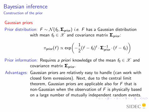
Gaussian priors
Prior distribution: F ∼ N (f0,Σprior) i.e. F has a Gaussian distributionwith mean f0 ∈X and covariance matrix Σprior:
πprior(f ) ∝ exp
(−1
2(f − f0)t ·Σ−1
prior · (f − f0)
)Prior information: Requires a priori knowledge of the mean f0 ∈X and
covariance matrix Σprior.
Advantages: Gaussian priors are relatively easy to handle (can work withclosed form exressions). Next, due to the central limittheorem, Gaussian priors are applicable also for F that isnon-Gaussian when the observation of F is physically basedon a large number of mutually independent random events.

Bayesian inferenceConstruction of the prior
Gibbs priors
Prior distribution: πprior(f ) ∝ exp(−µS(f )
).
Prior information: Requires a priori knowledge of µ > 0 and the functionalS : X → R+.
Advantages: Appropriate choice of S allows us to create priors thatencode the same a priori information as in classicalregularisation theory.
Disadvantages: f 7→ πprior(f ) can be interpreted as a proper probabilitydensity distribution only under certain circumstances, e.g. ifS(f ) =
∥∥L · f∥∥`2 then ker L = {0} needs to hold.
Bayesian inferenceConstruction of the prior
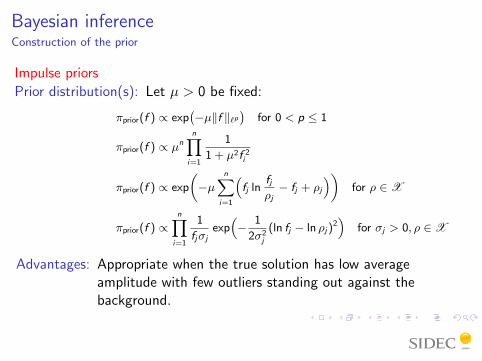
Impulse priors
Prior distribution(s): Let µ > 0 be fixed:
πprior(f ) ∝ exp`−µ‖f ‖`p
´for 0 < p ≤ 1
πprior(f ) ∝ µnnY
i=1
1
1 + µ2f 2i
πprior(f ) ∝ exp
„−µ
nXi=1
“fj ln
fjρj− fj + ρj
”«for ρ ∈ X
πprior(f ) ∝nY
i=1
1
fjσjexp“− 1
2σ2j
(ln fj − ln ρj)2”
for σj > 0, ρ ∈ X
Advantages: Appropriate when the true solution has low averageamplitude with few outliers standing out against thebackground.
Bayesian inferenceConstruction of the prior
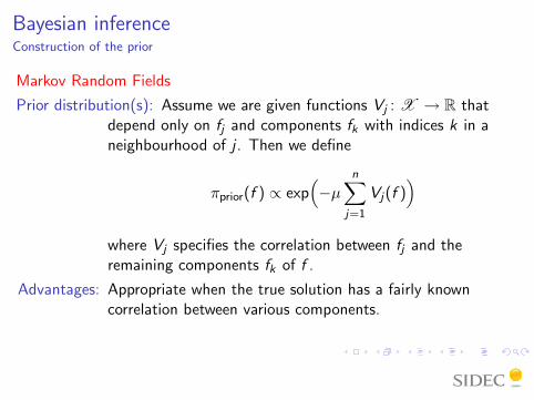
Markov Random Fields
Prior distribution(s): Assume we are given functions Vj : X → R thatdepend only on fj and components fk with indices k in aneighbourhood of j . Then we define
πprior(f ) ∝ exp(−µ
n∑j=1
Vj(f ))
where Vj specifies the correlation between fj and theremaining components fk of f .
Advantages: Appropriate when the true solution has a fairly knowncorrelation between various components.
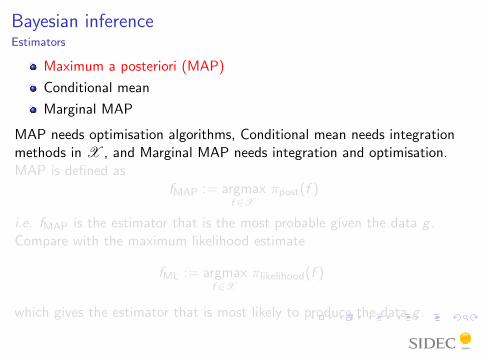
Bayesian inferenceEstimators
Maximum a posteriori (MAP)
Conditional mean
Marginal MAP
MAP needs optimisation algorithms, Conditional mean needs integrationmethods in X , and Marginal MAP needs integration and optimisation.MAP is defined as
fMAP := argmaxf ∈X
πpost(f )
i.e. fMAP is the estimator that is the most probable given the data g .Compare with the maximum likelihood estimate
fML := argmaxf ∈X
πlikelihood(f )
which gives the estimator that is most likely to produce the data g .
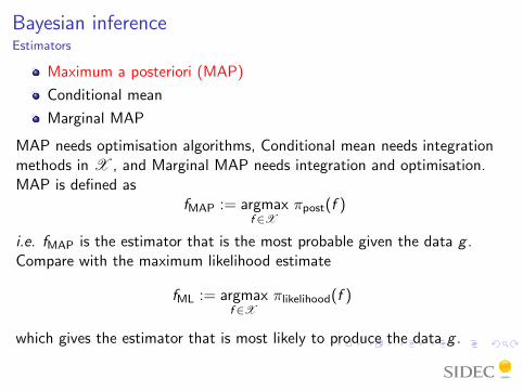
Bayesian inferenceRelation to classical regularisation theory
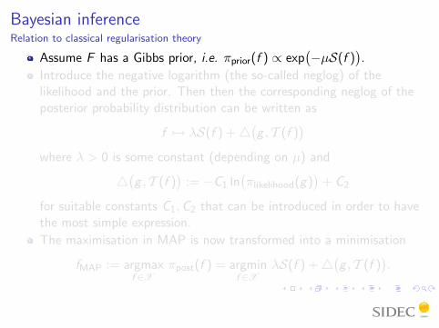
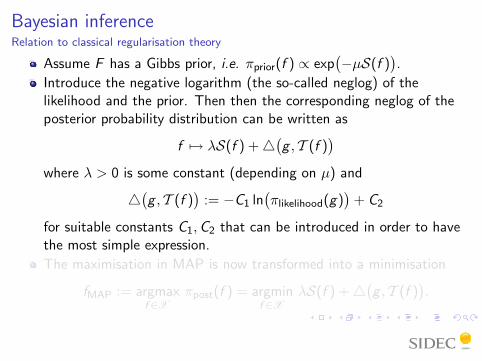
Assume F has a Gibbs prior, i.e. πprior(f ) ∝ exp(−µS(f )
).
Introduce the negative logarithm (the so-called neglog) of thelikelihood and the prior. Then then the corresponding neglog of theposterior probability distribution can be written as
f 7→ λS(f ) +4(g , T (f )
)where λ > 0 is some constant (depending on µ) and
4(g , T (f )
):= −C1 ln
(πlikelihood(g)
)+ C2
for suitable constants C1,C2 that can be introduced in order to havethe most simple expression.
The maximisation in MAP is now transformed into a minimisation
fMAP := argmaxf ∈X
πpost(f ) = argminf ∈X
λS(f ) +4(g , T (f )
).
Bayesian inferenceRelation to classical regularisation theory
Assume F has a Gibbs prior, i.e. πprior(f ) ∝ exp(−µS(f )
).
Introduce the negative logarithm (the so-called neglog) of thelikelihood and the prior. Then then the corresponding neglog of theposterior probability distribution can be written as
f 7→ λS(f ) +4(g , T (f )
)where λ > 0 is some constant (depending on µ) and
4(g , T (f )
):= −C1 ln
(πlikelihood(g)
)+ C2
for suitable constants C1,C2 that can be introduced in order to havethe most simple expression.
The maximisation in MAP is now transformed into a minimisation
fMAP := argmaxf ∈X
πpost(f ) = argminf ∈X
λS(f ) +4(g , T (f )
).
Advantages of Bayesian inference vs. classicalregularisation theory
Explicit account of the errors and noise.
A large class of priors via explicit or implicit modelling, e.g. morespecific and specialised priors can be created through introduction ofhidden variables.
A coherent approach to combine information content of the data andpriors.
Selection of regularisation parameter (which in the Bayesian case arethe unknown parameters in the prior) and multi-componentreconstruction problems can be dealt with systematically byhyperparameters.
Image processing operations, such as segmentation and labelling, canbe includes in the reconstruction by hidden variables.
Acknowledgments
Mathematics researchDr. Hans Rullgard, Department of Mathematics, Stockholm UniversityProf. Jan Boman, Department of Mathematics, Stockholm UniversityProf. Jan-Olov Stromberg, Department of Mathematics, Royal Institute of TechnologyProf. Todd Quinto, Department of Mathematics, Tufts universityProf. Dr. Alfred K. Louis, Numerische Mathematik, Universitat des SaarlandesProf. Ali Mohammad-Djafari, CNRS, ParisProf. Peter Maass, Zentrum fur Technomathematik, Universitat Bremen
Physics research & software developmentDr. Duccio Fanelli, Dipartimento di Energetica ’Sergio Stecco’, University of FlorenceDr. Hans Rullgard, Department of Mathematics, Stockholm UniversityScientists at Sidec Research & Development
Electron tomographyProf. Ulf Skoglund, Department of Cell and Molecular Biology, Karolinska InstitutetDr. Sara Sandin, MRC, CambridgeProf. Roger Kornberg, Stanford University Medical School, StanfordScientists at Sidec Protein Tomography lab.