Embed Size (px)
Citation preview
ISSN 1937 - 1055
VOLUME 3, 2015
INTERNATIONAL JOURNAL OF
MATHEMATICAL COMBINATORICS
EDITED BY
THE MADIS OF CHINESE ACADEMY OF SCIENCES AND
ACADEMY OF MATHEMATICAL COMBINATORICS & APPLICATIONS
September, 2015
Vol.3, 2015 ISSN 1937-1055
International Journal of
Mathematical Combinatorics
Edited By
The Madis of Chinese Academy of Sciences and
Academy of Mathematical Combinatorics & Applications
September, 2015
Aims and Scope: The International J.Mathematical Combinatorics (ISSN 1937-1055)
is a fully refereed international journal, sponsored by the MADIS of Chinese Academy of Sci-
ences and published in USA quarterly comprising 100-150 pages approx. per volume, which
publishes original research papers and survey articles in all aspects of Smarandache multi-spaces,
Smarandache geometries, mathematical combinatorics, non-euclidean geometry and topology
and their applications to other sciences. Topics in detail to be covered are:
Smarandache multi-spaces with applications to other sciences, such as those of algebraic
multi-systems, multi-metric spaces,· · · , etc.. Smarandache geometries;
Topological graphs; Algebraic graphs; Random graphs; Combinatorial maps; Graph and
map enumeration; Combinatorial designs; Combinatorial enumeration;
Differential Geometry; Geometry on manifolds; Low Dimensional Topology; Differential
Topology; Topology of Manifolds; Geometrical aspects of Mathematical Physics and Relations
with Manifold Topology;
Applications of Smarandache multi-spaces to theoretical physics; Applications of Combi-
natorics to mathematics and theoretical physics; Mathematical theory on gravitational fields;
Mathematical theory on parallel universes; Other applications of Smarandache multi-space and
combinatorics.
Generally, papers on mathematics with its applications not including in above topics are
also welcome.
It is also available from the below international databases:
Serials Group/Editorial Department of EBSCO Publishing
10 Estes St. Ipswich, MA 01938-2106, USA
Tel.: (978) 356-6500, Ext. 2262 Fax: (978) 356-9371
http://www.ebsco.com/home/printsubs/priceproj.asp
and
Gale Directory of Publications and Broadcast Media, Gale, a part of Cengage Learning
27500 Drake Rd. Farmington Hills, MI 48331-3535, USA
Tel.: (248) 699-4253, ext. 1326; 1-800-347-GALE Fax: (248) 699-8075
http://www.gale.com
Indexing and Reviews: Mathematical Reviews (USA), Zentralblatt Math (Germany), Refer-
ativnyi Zhurnal (Russia), Mathematika (Russia), Directory of Open Access (DoAJ), Interna-
tional Statistical Institute (ISI), International Scientific Indexing (ISI, impact factor 1.416),
Institute for Scientific Information (PA, USA), Library of Congress Subject Headings (USA).
Subscription A subscription can be ordered by an email directly to
Linfan Mao
The Editor-in-Chief of International Journal of Mathematical Combinatorics
Chinese Academy of Mathematics and System Science
Beijing, 100190, P.R.China
Email: [email protected]
Price: US$48.00

Editorial Board (3nd)
Editor-in-Chief
Linfan MAO
Chinese Academy of Mathematics and System
Science, P.R.China
and
Academy of Mathematical Combinatorics &
Applications, USA
Email: [email protected]
Deputy Editor-in-Chief
Guohua Song
Beijing University of Civil Engineering and
Architecture, P.R.China
Email: [email protected]
Editors
Said Broumi
Hassan II University Mohammedia
Hay El Baraka Ben M’sik Casablanca
B.P.7951 Morocco
Junliang Cai
Beijing Normal University, P.R.China
Email: [email protected]
Yanxun Chang
Beijing Jiaotong University, P.R.China
Email: [email protected]
Jingan Cui
Beijing University of Civil Engineering and
Architecture, P.R.China
Email: [email protected]
Shaofei Du
Capital Normal University, P.R.China
Email: [email protected]
Baizhou He
Beijing University of Civil Engineering and
Architecture, P.R.China
Email: [email protected]
Xiaodong Hu
Chinese Academy of Mathematics and System
Science, P.R.China
Email: [email protected]
Yuanqiu Huang
Hunan Normal University, P.R.China
Email: [email protected]
H.Iseri
Mansfield University, USA
Email: [email protected]
Xueliang Li
Nankai University, P.R.China
Email: [email protected]
Guodong Liu
Huizhou University
Email: [email protected]
W.B.Vasantha Kandasamy
Indian Institute of Technology, India
Email: [email protected]
Ion Patrascu
Fratii Buzesti National College
Craiova Romania
Han Ren
East China Normal University, P.R.China
Email: [email protected]
Ovidiu-Ilie Sandru
Politechnica University of Bucharest
Romania
ii International Journal of Mathematical Combinatorics
Mingyao Xu
Peking University, P.R.China
Email: [email protected]
Guiying Yan
Chinese Academy of Mathematics and System
Science, P.R.China
Email: [email protected]
Y. Zhang
Department of Computer Science
Georgia State University, Atlanta, USA
Famous Words:
It is at our mother’s knee that we acquire our noblest and truest and highest
ideals, but there is seldom any money in them.
By Mark Twain, an American writer.
International J.Math. Combin. Vol.3(2015), 01-32
A Calculus and Algebra Derived from Directed Graph Algebras
Kh.Shahbazpour and Mahdihe Nouri
(Department of Mathematics, University of Urmia, Urmia, I.R.Iran, P.O.BOX, 57135-165)
E-mail: [email protected]
Abstract: Shallon invented a means of deriving algebras from graphs, yielding numerous
examples of so-called graph algebras with interesting equational properties. Here we study
directed graph algebras, derived from directed graphs in the same way that Shallon’s undi-
rected graph algebras are derived from graphs. Also we will define a new map, that obtained
by Cartesian product of two simple graphs pn, that we will say from now the mah-graph.
Next we will discuss algebraic operations on mah-graphs. Finally we suggest a new algebra,
the mah-graph algebra (Mah-Algebra), which is derived from directed graph algebras.
Key Words: Direct product, directed graph, Mah-graph, Shallon algebra, kM-algebra
AMS(2010): 08B15, 08B05.
§1. Introduction
Graph theory is one of the most practical branches in mathematics. This branch of mathematics
has a lot of use in other fields of studies and engineering, and has competency in solving lots of
problems in mathematics. The Cartesian product of two graphs are mentioned in[18]. We can
define a graph plane with the use of mentioned product, that can be considered as isomorphic
with the plane Z+ ∗ Z
+.
Our basic idea is originated from the nature. Rivers of one area always acts as unilateral
courses and at last, they finished in the sea/ocean with different sources. All blood vessels from
different part of the body flew to heart of beings. The air-lines that took off from different part
of world and all landed in the same airport. The staff of an office that worked out of home and
go to the same place, called Office, and lots of other examples give us a new idea of directed
graphs. If we consider directed graphs with one or more primary point and just one conclusive
point, in fact we could define new shape of structures.
A km-map would be defined on a graph plane, made from Cartesian product of two simple
graphs pn ∗pn. The purpose of this paper is to define the kh-graph and study of a new structure
that could be mentioned with the definition of operations on these maps.
The km-graph could be used in the computer logic, hardware construction in smaller size
with higher speed, in debate of crowded terminals, traffics and automations. Finally by rewriting
1Received January 1, 2015, Accepted August 6, 2015.
2 Kh.Shahbazpour and Mahdihe Nouri
the km-graphs into mathematical formulas and identities, we will have interesting structures
similar to Shallon’s algebra (graph algebra).
At the first part of paper, we will study some preliminary and essential definitions. In sec-
tion 3 directed graphs and directed graph algebras are studied. The graph plane and mentioned
km-graph and its different planes and structures would be studied in section 4.
§2. Basic Definitions and Structures
In this section we provide the basic definitions and theorems for some of the basic structures
and ideas that we shall use in the pages ahead. For more details, see [18], [23], [12].
Let A be a set and n be a positive integer. We define An to be the set of all n-tuples of
A, and A0 = ∅. The natural number n is called the rank of the operation, if we call a map
φ : An → A an n − ary operation on A. Operations of rank 1 and 2 are usually called unary and
binary operations, respectively. Also for all intends and purposes, nullary operations (as those
of rank 0 are often called) are just the elements of A. They are frequently called constants.
Definition 2.1 An algebra is a pair < A, F > in which A is a nonempty set and F =< fi :
i ∈ I > is a sequence of operations on A, indexed by some set I. The set A is the universe of
the algebra, and the fi’s are the fundamental or basic operations.
For our present discussion, we will limit ourselves to finite algebras, that is, those whose
universes are sets of finite cardinality . The equational theory of an algebra is the set consisting
of all equations true in that algebra. In the case of groups, one such equation might be the
associative identity. If there is a finite list of equations true in an algebra from which all
equations true in the algebra can be deduced, we say the algebra is finitely based. For example
in the class of one-element algebras, each of those is finitely based and the base is simply the
equation x ≈ y. We typically write A to indicate the algebra < A, F > expect when doing so
causes confusion. For each algebra A, we define a map ρ : I → ω by letting ρ(i) = rank(Fi)
for every i ∈ I. The set I is called the set of operation symbols. The map ρ is known as the
signature of the algebra A and it simply assigns to each operation symbol the natural number
which is its rank. When a set of algebras share the same signature, we say that they are similar
or simply state their shared signature.
If κ is a class of similar algebras, we will use the following notations:
H(κ) represents the class of all homomorphic images of members of κ;
S(κ) represents the class of all isomorphic images of sub algebras of members of κ;
P (κ) represents the class of all direct products of system of algebras belonging to κ.
Definition 2.2 The class ν of similar algebras is a variety provided it is closed with respect to
the formation of homomorphic images, sub algebras and direct products.
According to a result of Birkhoff ( Theorem 2.1), it turns out that ν is a variety precisely
if it is of the form HSP (κ) for some class κ of similar algebras. We use HSP (A) to denote the
A Calculus and Algebra Derived from Directed Graph Algebras 3
variety generated by an algebra A. The equational theory of an algebra is the set consisting of
all equations true in that algebra. In order to introduce the notion of equational theory, we
begin by defining the set of terms.
Let T (X) be the set of all terms over the alphabet X = {x0, x1, · · · } using juxtaposition
and the symbol ∞. T (X) is defined inductively as follows:
(i) every xi, (i = 0, 1, 2, · · · ) (also called variables) and ∞ is a term;
(ii) if t and t′ are terms, then (tt′) is a term;
(iii) T (X) is the set of all terms which can be obtained from (i) and (ii) in finitely many
steps.
The left most variable of a term t is denoted by Left(t). A term in which the symbol ∞occurs is called trivial. Let T ′(X) be the set of all non-trivial terms. To every non-trivial term
t we assign a directed graph G(t) = (V (t), R(t)) where V (t) is the set of all variables and R(t)
is defined inductively by R(t) = ∅ if t ∈ X and R(tt′) = R(t)∪R(t′)∪{Left(t), Left(t′)}. Note
that G(t) always a connected graph.
An equation is just an ordered pair of terms. We will denote the equation (s, t) by s ≈ t.
We say an equation s ≈ t is true in an algebra A provided s and t have the same signature. In
this case, we also say that A is a model of s ≈ t, which we will denote by A |= s ≈ t.
Let κ be a class of similar algebras and let Σ be any set of equations of the same similarity
type as κ. We say that κ is a class of models Σ(or that Σ is true in κ) provided A |= s ≈ t ) for
all algebras A found in κ and for all equations s ≈ t found in Σ. We use κ |= Σ to denote this,
and we use ModΣ to denote the class of all models of Σ.
The set of all equations true in a variety ν ( or an algebra A) is known as the equational
theory of ν (respectively, A). If Σ is a set of equations from which we can derive the equation
s ≈ t, we write Σ ⊢ s ≈ t and we say s ≈ t is derivable from Σ. In 1935, Garrett Birkhoff proved
the following theorem:
Theorem 2.1 (Bikhoffs HSP Theorem) Let ν be a class of similar algebras. Then ν is a
variety if and only if there is a set σ of equations and a class κ of similar algebras so that
ν = HSP (κ) = ModΣ.
From this theorem, we have a clear link between the algebraic structures of the variety ν
and its equational theory.
Definition 2.3 A set Σ of equations is a base for the variety ν (respectively, the algebra A)
provided ν (respectively, HSP(A)) is the class of all models of Σ.
Thus an algebra A is finitely based provided there exists a finite set Σ of equations such
that any equation true in A can be derived from Σ. That is, if A |= s ≈ t and Σ is a finite base
of the equational theory of A, then Σ ⊢ s ≈ t. If a variety or an algebra does not have a finite
base, we say that it fails to finitely based and we call it non-finitely based.
We say an algebra is locally finite provided each of its finitely generated sub algebras is
finite, and we say a variety is locally finite if each of its algebras is locally finite.
A useful fact is the following:
4 Kh.Shahbazpour and Mahdihe Nouri
Theorem 2.2 Every variety generated by a finite algebra is locally finite.
Thus if A is an inherently nonfinitely based finite algebra that is a subset of B, where
B is also finite, then B must also be inherently nonfinitely based. It is in this way that the
property of being inherently nonfinitely based is contagious. In an analogous way, we define an
inherently non-finitely based variety ϑ as one in which the following conditions occur:
(i) ϑ has a finite signature;
(ii) ϑ is locally finite;
(iii) ϑ is not included in any finitely based locally finite variety.
Let ν be a variety and let n ∈ ω. The class ν(n) of algebras is defined by the following
condition:
An algebra B is found in ν(n) if and only if every sub algebra of B with n or fewer generators
belongs to ν. Equivalently, we might think of ν(n) as the variety defined by the equations true
in ν(n) that have n or fewer variables. Notice that (ν ⊆ · · · ⊆ ν(n+1) ⊆ ν(n) ⊆ ν(n−1) ⊆ · · · )and ν =
⋂nu(n)
n∈ω .
A nonfinitely based algebra A might be nonfinitely based in a more infectious manner:
It might turn out that if A is found in HSP (B), where B is a finite algebra, then B is also
nonfinitely based. This leads us to a stronger non finite basis concept.
Definition 2.4 An algebra A is inherently non-finitely based provided:
(i) A has only finitely many basic operations;
(ii) A belongs to some locally finite operations;
(iii) A belong to no locally finite variety which is finitely based.
In an analogous way, we say that a locally finite variety v of finite signature is inherently
nonfinitely based provided it is not included in any finitely based locally finite variety. In
[2], Birkhoff observed that v(n) is finitely based whenever v is a locally finite variety of finite
signature. As an example, let v be a locally finite variety of finite signature. If the only basic
operations of v are either of rank 0 or rank 1, then every equation true in v can have at most
two variables. In other words, v = v(2) and so v is finitely based. From Birkhoff’s observation,
we have the following as pointed out by McNulty in [15]:
Theorem 2.3 Let v be locally finite variety with a finite signature. Then the following condi-
tions are equivalent:
(i) v is inherently non-finitely based;
(ii) The variety v(n) is not locally finite for any natural number n;
(iii) For arbitrary large natural numbers N , there exists a non-locally finite algebra BN
whose N -generated sub algebras belong to v.
Thus to show that a locally finite variety v of finite signature is inherently nonfinitely
based, it is enough to construct a family of algebras Bn (for each n ∈ ω ) so that each Bn fails
to be locally finite and is found inside v(n).

A Calculus and Algebra Derived from Directed Graph Algebras 5
In 1995, Jezek and McNulty produced a five element commutative directoid and showed
that while it is nonfinitely based, it fails to be inherently based [17]. This resolved the original
question of jezek and Quackenbush but did not answer the following:
Is there a finite commutative directed that is inherently non-finitely based?
In 1996, E.Hajilarov produced a six-element commutative directoid and asserted that it
is inherently based [5]. We will discuss an unresolved issue about Hajilarov’s directoid that
reopens its finite basis question. We also provide a partial answer to the modified question of
jezek and Quackenbush by constructing a locally finite variety of commutative directoids that
is inherently nonfinitely based.
A sub direct representation of an algebra A is a system < hi : i ∈ I > of homomorphisms, all
with domain A, that separates the points of A: that is, if a and b are distinct elements of A, ten
there is at least one i ∈ I so that hi(a) 6= hi(b). The algebra hi(A) are called subdirectfactors
of the representation. Starting with a complicated algebra A, one way to better understand its
structure is to analyze a system < hi(A) i ∈ I > of potentially less complicated homomorphic
image, and a sub direct representation of A provides such a system.
The residual bound of a variety ϑ is the least cardinal κ (should one exist ) such that for
every algebra A ∈ ϑ there is a sub direct representation < hii ∈ I > of A such that each sub
direct factor has fewer than κ elements. If a variety ν of finite signature has a finite residual
bound, it also satisfies the following condition: there is a finite set S of finite algebras belonging
to ϑ so that every algebra in ϑ has a sub direct representation using only sub direct factors
from s.
According to a result of Robert Quackenbush, if a variety generated by a finite algebra has
an infinite sub directedly irreducible member, it must also have arbitrarily large finite once [20].
In 1981, Wieslaw Dziobiak improved this result by showing that the same holds in any locally
finite variety [3]. A Problem of Quackenbush asks whether there exists a finite algebra such
that the variety it generates contains infinitely many distinct (up to isomorphism) sub directly
irreducible members but no infinite ones. One of the thing Ralph McKenzie did in [13] was to
provide an example of 4-element algebra of countable signature that generates a variety with
this property. Whether or not this is possible with an algebra with only finitely many basic
operations is not yet know.
If all of the sub directly irreducible algebra in a variety are finite, we say that the variety is
residual finite. Starting with a finite algebra, there is no guarantee that the variety it generates
is residually finite, nor that the algebra is finitely based. The relationship between these three
finiteness conditions led to the posing of the following problem in 1976:
Is every finite algebra of finite signature that generates a variety with a finite a finite
residual bound finitely based?
Bjarni Jonsson posed this problem at a meeting at a meeting at the Mathematical Research
Institute in Oberwolfach while Robert Park offered it as a conjecture in his PH.D. dissertation
[19]. At the time this problem was framed, essentially only five nonfinitely based finite algebras
were known. Park established that none of these five algebras could be a counterexample. In
6 Kh.Shahbazpour and Mahdihe Nouri
the ensuing years our supply of nonfinitely based finite algebras has become infinite and varied,
yet no counterexample is known. Indeed, Ros Willard [26] has offered a 50 euro reward for
the first published example of such an algebra. In chapter 2, we show that a wide class of
algebras known to be nonfinitely based will not supply such an example. It is still an open
problem whether some of the nonfinitely based finite algebras known today generate varieties
with finite residual bound. while the condition of generating a variety with a finite residual
bound could well be sufficient to ensure that a finite algebra is finitely based, it is in its own
right a very subtle property of finite algebras. Indeed, Ralph McKenzie has shown that there
is no algorithm for recognizing when a finite algebra has this property [13]. The last question
motivating our research was originally formulated in 1976 by Eilenberg and Schutzenberger [4].
In their investigation of pseudo varieties, they ask, If ϑ is a variety generated by a finite algebra,
W is a finitely based variety, and ϑ and W share the same finite algebras, must ϑ be finitely
based?
To answer this question in the negative, one would need to supply a finite, nonfinitely
based algebra to generate ϑ and a finitely based variety W so that ϑ and W have the same
finite algebras. McNulty, Szekely, and Willard have proven that no counterexample can be found
among a wide class of finite, non finitely based algebras [26]; furthermore they noted that this
property also cannot be recognized by any algorithm.We show that the locally finite, inherently
based variety of commutative directoids we construct will fail to yield a counterexample if it is
shown to be generated by a finite algebra.
§3. Directed Graphs and Directed Graph Algebras
Definition 3.1 A graph G is a triple consisting of a vertex set V (G), an edge set E(G), and
a relation that associates with each two vertexes called its conclusive points.
Definition 3.2 A path in the directed graph (v, E) is an ordered (n + 1)−tuple (x1, · · · , xn+1)
such that (xi, xi+1) ∈ E for all i = 1, · · · , n. The path (x1, ..., xn+1) has length n. A cycle is
a path from some vertex to itself. Given a graph G and x ∈ VG, [x〉G, (or just [x〉, when G
is clear), is the set of y ∈ VG such that there is a path from x to y in G. A directed graph is
acyclic if it contains no cycles. A directed graph (V, E) is loop-free if there is no cycle of length
1, that is if there is no x ∈ V such that (x, x) ∈ E. A directed graph (V, E) is looped if there is
a loop at every vertex, that is if (x, x) ∈ E for every x ∈ V.
Definition 3.3 A directed graph or digraph G =< V, E > is a triple consisting of a nonempty
set V (G) of elements called vertexes, together with a set E(G) of ordered pairs from V ×V → V ,
called edges, and a map that assigning to each edge an ordered pair of vertexes.
Thus our directed graphs do not allow multiple edges, but they do allow edges of the form
(x, x) (that is, we allow vertexes to be looped). Given a directed graph G, we can refer to the
vertex set and edge set of G as VG and EG, respectively. Let us say that G is a subgraph of
G if VG ⊆ VG and EG = EG
⋂
(VG × VG). When we draw a directed graph, we generally draw
the edge (x, y) as an arrow from vertex x to y. When drawing an undirected graph, we simply
A Calculus and Algebra Derived from Directed Graph Algebras 7
draw the edge (x, y) as a line from x to y; since we know that (y, x) must also be in the graph
edge set, there is no question of which way the edge goes. Let us call any variety generated by
directed graph algebras a directed graph variety. As noted in [25], any directed graph variety ν
contains A(G) for all G that are direct products, subgraphs, disjoint unions, directed unions and
homomorphic images of directed graphs underlying algebra in ν. More generally, any variety
is closed under homomorphisms, sub algebras and direct products. We shall need this more
general fact to obtain the results in section. The following definition is from [25].
Definition 3.4([25]) Let G = (V, E) be a directed graph. The directed graph algebra A(G) is
the algebra with underlying set {v⋃∞}, where ∞ /∈ V , and two basic operations: one nullary
operation, also denoted by ∞, which has value ∞, and one binary operation, sometimes called
multiplication, denoted by juxtaposition, which is given by
(u, v) =
u if(u, v) ∈ E
∞ otherwise
Let G =< V, E > be a complete undirected graph. We define a tournament T as an algebra
with universe V ∪ {∞} ( where ∞ /∈ V ) and binary relation ։ so that for distinct x, y ∈ V
exactly one of x ։ y and y ։ x is true. We make each edge directed using the relation ։,
that is, we make the edge between x and y directed toward y if and only if x ։ y. We can then
make ։ into a binary operation as follows:
x.y = y.x =
x ifx ։ y
∞ otherwise
The relation x ։ y is generally read as ”x defeats y” or ” y loses to x” in the tournament T .
Notice that in tournament we require a directed edge between any two distinct vertexes. When
we draw a tournament, we will represent the ordered edge between any two distinct vertexes.
When we draw a tournament, we will represent the ordered pair (x, y) ∈։ as vertexes joined
by a double-headed arrow pointing away from x.y.
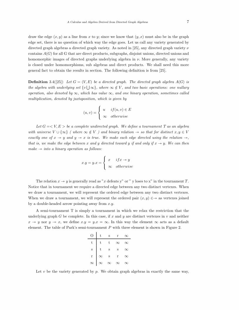
A semi-tournament T is simply a tournament in which we relax the restriction that the
underlying graph G be complete. In this case, if x and y are distinct vertexes in v and neither
x ։ y nor y ։ x, we define x.y = y.x = ∞. In this way the element ∞ acts as a default
element. The table of Park’s semi-tournament P with three element is shown in Figure 2.
O t s r ∞t t t ∞ ∞s t s s ∞r ∞ s r ∞∞ ∞ ∞ ∞ ∞
Let v be the variety generated by p. We obtain graph algebras in exactly the same way,
8 Kh.Shahbazpour and Mahdihe Nouri
except that in a graph algebra the underlying G is an undirected graph . one difference between
our terminology and the terminology of the authors of [25] is that they refer to algebras A(G)
defined as graph algebras, while we refer to such algebras as directed graph algebra. Our
purpose in doing so is to avoid confusion with the (undirected) graph algebra of [25]. Let T (X)
be the set of all terms over a set X of variables in the type of directed graph algebras. We shall
make frequent use of the following definition and lemma from Kiss-poschel-prohle [25].
Definition 3.5([25]) For t ∈ T (X), the term graph G(t) = (V (t), E(t)) is the directed graph
defined as follows. v(t) is the set of variables that appear in t. E(t) is defined inductively as
follows:
E(t) = φ if t is a variable, and E(ts) = E(t) ∪ E(S)⋃
(L(t), L(s)), where L(t) is the
leftmost variable that appears in t. The rooted graph derived from t is (G(t), L(t)).
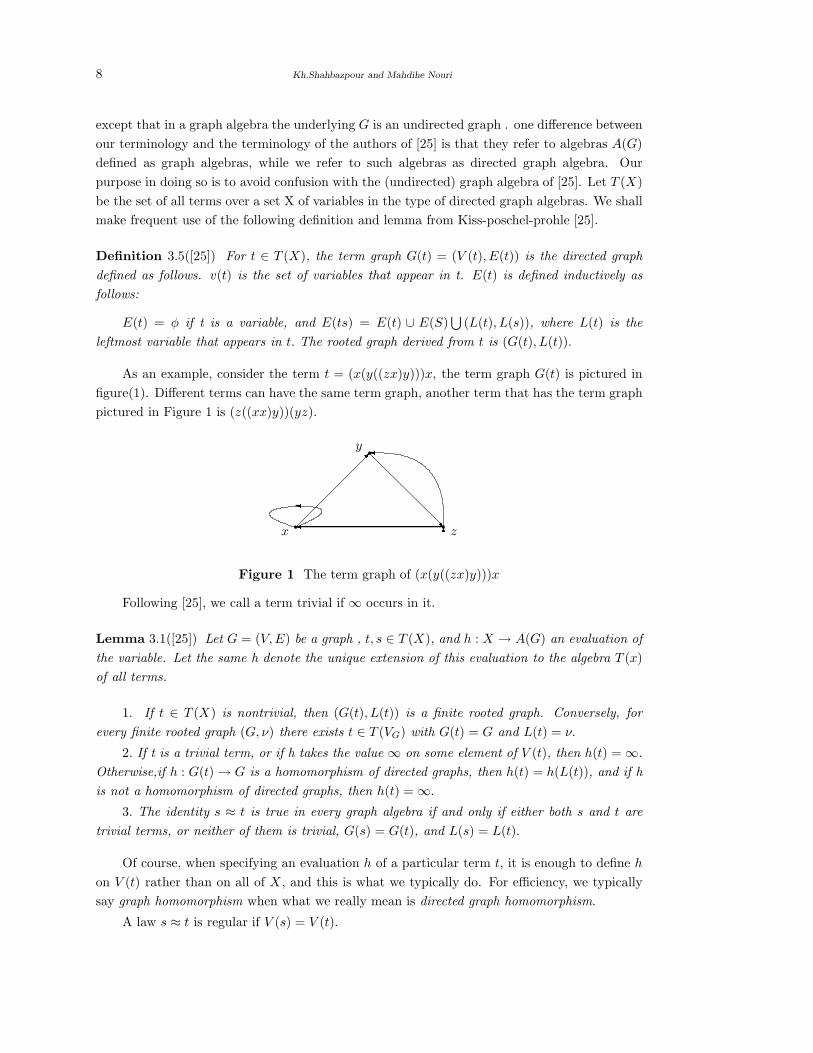
As an example, consider the term t = (x(y((zx)y)))x, the term graph G(t) is pictured in
figure(1). Different terms can have the same term graph, another term that has the term graph
pictured in Figure 1 is (z((xx)y))(yz).
R� 6� �� y
x z
Figure 1 The term graph of (x(y((zx)y)))x
Following [25], we call a term trivial if ∞ occurs in it.
Lemma 3.1([25]) Let G = (V, E) be a graph , t, s ∈ T (X), and h : X → A(G) an evaluation of
the variable. Let the same h denote the unique extension of this evaluation to the algebra T (x)
of all terms.
1. If t ∈ T (X) is nontrivial, then (G(t), L(t)) is a finite rooted graph. Conversely, for
every finite rooted graph (G, ν) there exists t ∈ T (VG) with G(t) = G and L(t) = ν.
2. If t is a trivial term, or if h takes the value ∞ on some element of V (t), then h(t) = ∞.
Otherwise,if h : G(t) → G is a homomorphism of directed graphs, then h(t) = h(L(t)), and if h
is not a homomorphism of directed graphs, then h(t) = ∞.
3. The identity s ≈ t is true in every graph algebra if and only if either both s and t are
trivial terms, or neither of them is trivial, G(s) = G(t), and L(s) = L(t).
Of course, when specifying an evaluation h of a particular term t, it is enough to define h
on V (t) rather than on all of X , and this is what we typically do. For efficiency, we typically
say graph homomorphism when what we really mean is directed graph homomorphism.
A law s ≈ t is regular if V (s) = V (t).
A Calculus and Algebra Derived from Directed Graph Algebras 9
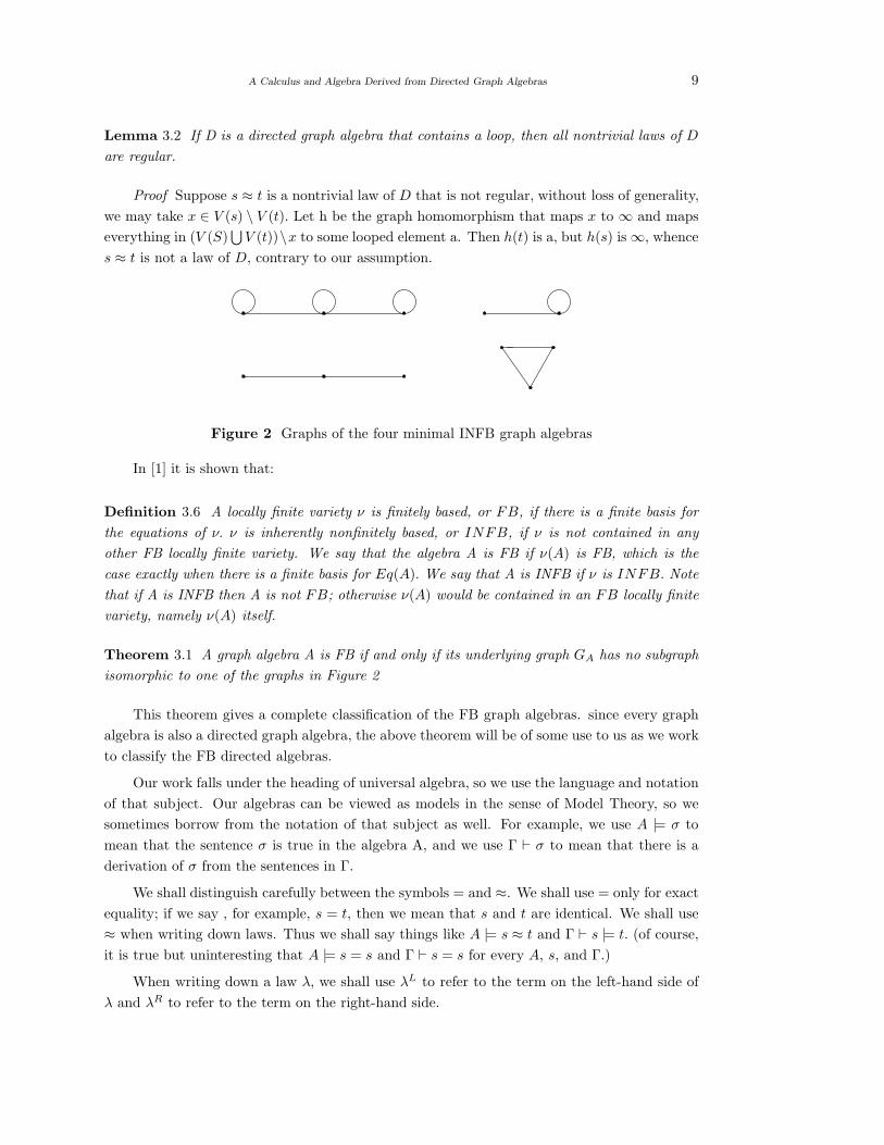
Lemma 3.2 If D is a directed graph algebra that contains a loop, then all nontrivial laws of D
are regular.
Proof Suppose s ≈ t is a nontrivial law of D that is not regular, without loss of generality,
we may take x ∈ V (s) \ V (t). Let h be the graph homomorphism that maps x to ∞ and maps
everything in (V (S)⋃
V (t))\x to some looped element a. Then h(t) is a, but h(s) is ∞, whence
s ≈ t is not a law of D, contrary to our assumption.
Figure 2 Graphs of the four minimal INFB graph algebras
In [1] it is shown that:
Definition 3.6 A locally finite variety ν is finitely based, or FB, if there is a finite basis for
the equations of ν. ν is inherently nonfinitely based, or INFB, if ν is not contained in any
other FB locally finite variety. We say that the algebra A is FB if ν(A) is FB, which is the
case exactly when there is a finite basis for Eq(A). We say that A is INFB if ν is INFB. Note
that if A is INFB then A is not FB; otherwise ν(A) would be contained in an FB locally finite
variety, namely ν(A) itself.
Theorem 3.1 A graph algebra A is FB if and only if its underlying graph GA has no subgraph
isomorphic to one of the graphs in Figure 2
This theorem gives a complete classification of the FB graph algebras. since every graph
algebra is also a directed graph algebra, the above theorem will be of some use to us as we work
to classify the FB directed algebras.
Our work falls under the heading of universal algebra, so we use the language and notation
of that subject. Our algebras can be viewed as models in the sense of Model Theory, so we
sometimes borrow from the notation of that subject as well. For example, we use A |= σ to
mean that the sentence σ is true in the algebra A, and we use Γ ⊢ σ to mean that there is a
derivation of σ from the sentences in Γ.
We shall distinguish carefully between the symbols = and ≈. We shall use = only for exact
equality; if we say , for example, s = t, then we mean that s and t are identical. We shall use
≈ when writing down laws. Thus we shall say things like A |= s ≈ t and Γ ⊢ s |= t. (of course,
it is true but uninteresting that A |= s = s and Γ ⊢ s = s for every A, s, and Γ.)
When writing down a law λ, we shall use λL to refer to the term on the left-hand side of
λ and λR to refer to the term on the right-hand side.
10 Kh.Shahbazpour and Mahdihe Nouri
Given a term t, l(t) is the length of t, defined by the following recursion:
l(t) =
1 if t is a single variable
l(r) + l(s) if t = rs.
Thus l(t) is the number of places at which variables occur in t.
When dealing with terms, it is expeditious to avoid writing down as many parentheses as
possible. Toward this end, we adopt the convention that sub terms will be grouped from the
left. Thus, for example, when we say
xy1y2...yn
we mean that
(· · · ((xy1)y2) · · · )yn.
When giving a derivation, we justify the steps as follows. When a step is justified by a
numbered entity, such as an equation or proposition, the number appears underneath the ≈ or
= on that step’s line in the proof. When the justification is something that does not have a
number, the justification appears in square brackets at the right end of the line.
In general, we use u, υ, w, x, y, and z for variables, s, t, and lowercase Greek letters for
terms and sub terms, lower case Greek letters for laws, and uppercase Greek letters for sets of
laws.
§4. km-Graphs
In this section we will define graph plane and then we will construct km-graphs. Next by
using the language and notation of universal algebra, we will define a new algebra derived from
directed graph algebras.
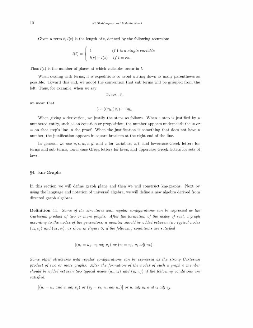
Definition 4.1 Some of the structures with regular configurations can be expressed as the
Cartesian product of two or more graphs. After the formation of the nodes of such a graph
according to the nodes of the generators, a member should be added between two typical nodes
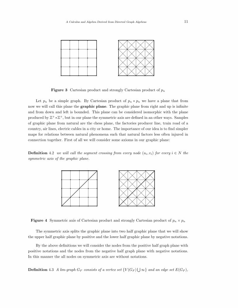
(ui, vj) and (uk, vl), as show in Figure 3, if the following conditions are satisfied
[(ui = uk, vl adj vj) or (vi = vl, ui adj uk)].
Some other structures with regular configurations can be expressed as the strong Cartesian
product of two or more graphs. After the formation of the nodes of such a graph a member
should be added between two typical nodes (uk, vl) and (ui, vj) if the following conditions are
satisfied:
[(ui = uk and vl adj vj) or (vj = vl, ui adj uk)] or ui adj uk and vl adj vj .
A Calculus and Algebra Derived from Directed Graph Algebras 11
Figure 3 Cartesian product and strongly Cartesian product of pn
Let pn be a simple graph. By Cartesian product of pn ∗ pn we have a plane that from
now we will call this plane the graphic plane. The graphic plane from right and up is infinite
and from down and left is bounded. This plane can be considered isomorphic with the plane
produced by Z+∗Z
+, but in our plane the symmetric axis are defined in an other ways. Samples
of graphic plane from natural are the chess plane, the factories producer line, train road of a
country, air lines, electric cables in a city or home. The importance of our idea is to find simpler
maps for relations between natural phenomena such that natural factors less often injured in
connection together. First of all we will consider some axioms in our graphic plane:
Definition 4.2 we will call the segment crossing from every node (ui, vi) for every i ∈ N the
symmetric axis of the graphic plane.
Figure 4 Symmetric axis of Cartesian product and strongly Cartesian product of pn × pn
The symmetric axis splits the graphic plane into two half graphic plane that we will show
the upper half graphic plane by positive and the lower half graphic plane by negative notations.
By the above definitions we will consider the nodes from the positive half graph plane with
positive notations and the nodes from the negative half graph plane with negative notations.
In this manner the all nodes on symmetric axis are without notations.
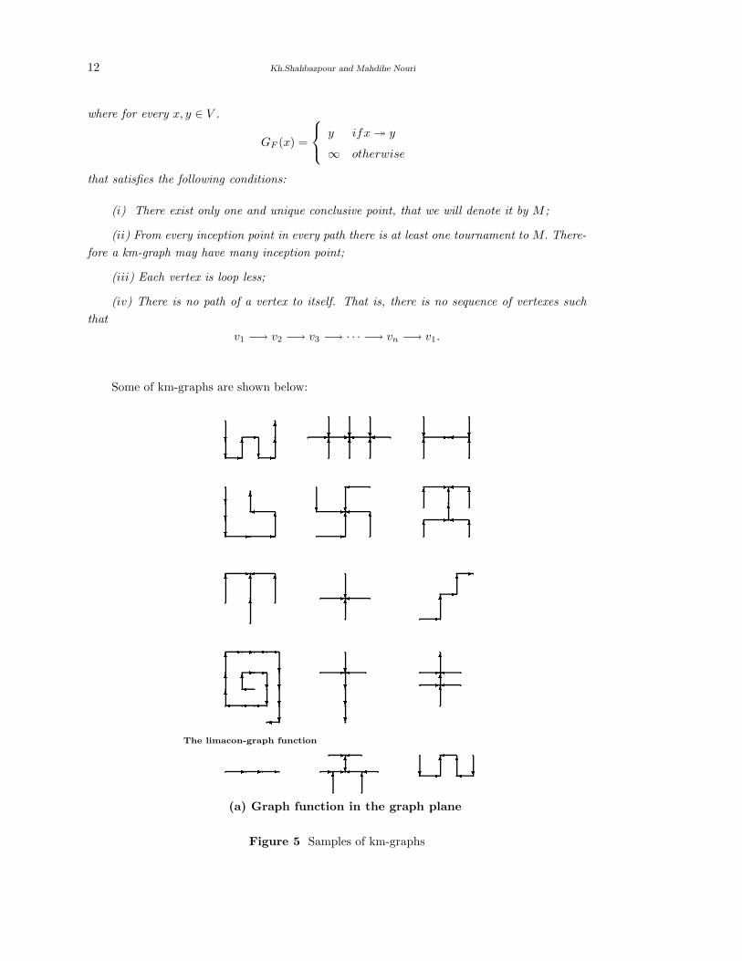
Definition 4.3 A km-graph GF consists of a vertex set {V (GF )⋃∞} and an edge set E(GF ),
12 Kh.Shahbazpour and Mahdihe Nouri
where for every x, y ∈ V .
GF (x) =
y ifx ։ y
∞ otherwise
that satisfies the following conditions:
(i) There exist only one and unique conclusive point, that we will denote it by M ;
(ii) From every inception point in every path there is at least one tournament to M. There-
fore a km-graph may have many inception point;
(iii) Each vertex is loop less;
(iv) There is no path of a vertex to itself. That is, there is no sequence of vertexes such
that
v1 −→ v2 −→ v3 −→ · · · −→ vn −→ v1.
Some of km-graphs are shown below:??-6-?-66 - -� �? ? ?6 6 6 -�? ?6 6???- -6�6 ? -�?-6 6� 6- 6�6- 6�66--6-6?6-�666- 6�----�6--??���666 ????� ????-� 666-�-�- - - --� �-6?�6 6 ?-6 ?�6�The limacon-graph function
(a) Graph function in the graph plane
Figure 5 Samples of km-graphs
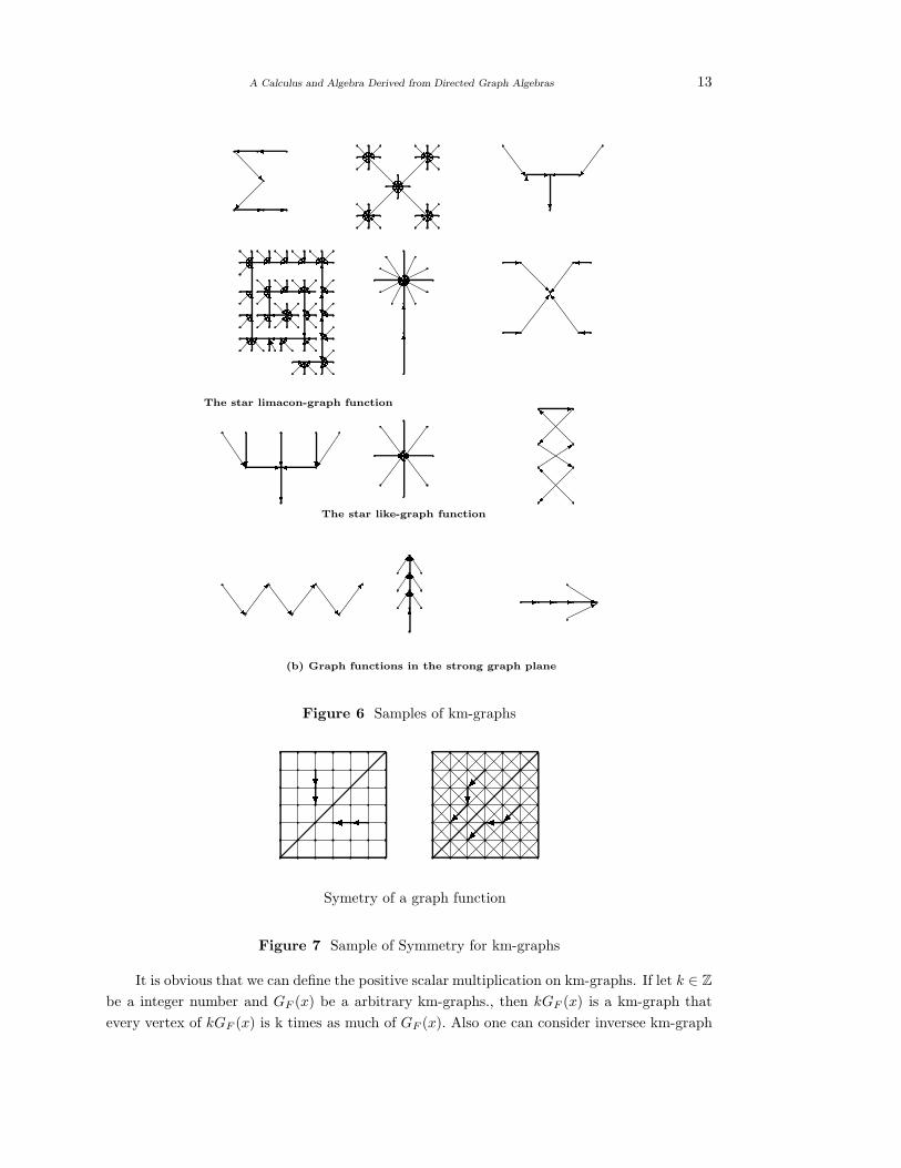
A Calculus and Algebra Derived from Directed Graph Algebras 13��R- - R RI I?-�6� 6?�-�-�6?�-�6?�RI -�?6RI w6-?� /�
----6?6?6??-6-6 --6 ??���66��66 �I6I�����?R?R?R?R?-R�-�-�-6�I6K 6I 6�I�I?�R?R?R�-6� ?R6�I 666?-���j*�KY - R ��- 7/o
The star limacon-graph function-�? ???^ � -�?6w/7o - sI 3IThe star like-graph function
w 7 w 7 w 7 6666�℄�℄�℄ --- -s*(b) Graph functions in the strong graph plane
Figure 6 Samples of km-graphs?? �� ? �Symetry of a graph function
Figure 7 Sample of Symmetry for km-graphs
It is obvious that we can define the positive scalar multiplication on km-graphs. If let k ∈ Z
be a integer number and GF (x) be a arbitrary km-graphs., then kGF (x) is a km-graph that
every vertex of kGF (x) is k times as much of GF (x). Also one can consider inversee km-graph
14 Kh.Shahbazpour and Mahdihe Nouri
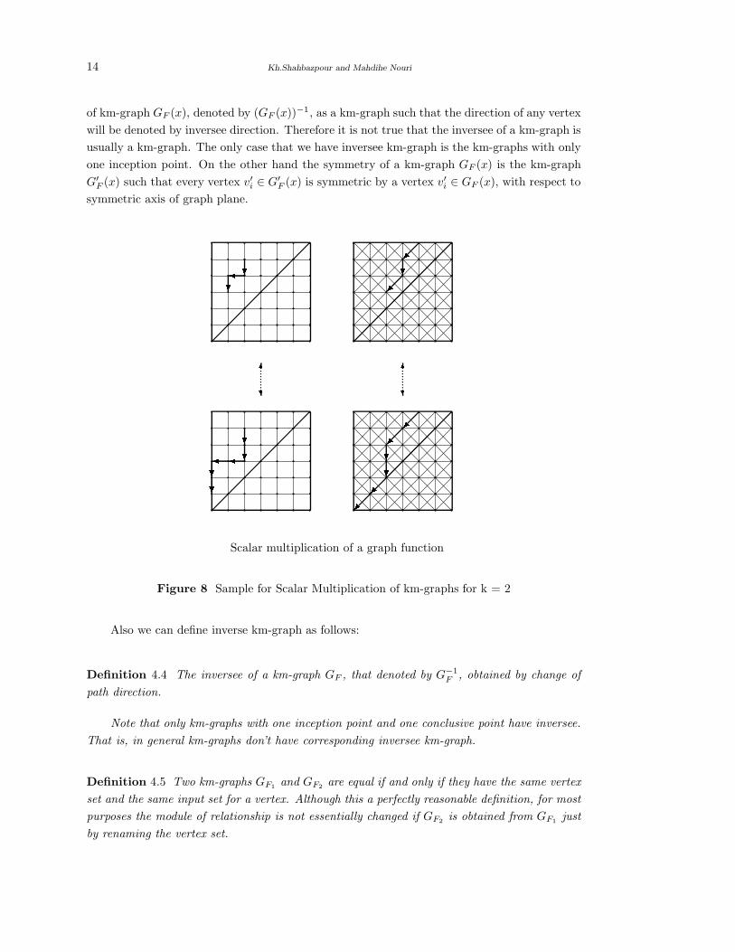
of km-graph GF (x), denoted by (GF (x))−1, as a km-graph such that the direction of any vertex
will be denoted by inversee direction. Therefore it is not true that the inversee of a km-graph is
usually a km-graph. The only case that we have inversee km-graph is the km-graphs with only
one inception point. On the other hand the symmetry of a km-graph GF (x) is the km-graph
G′F (x) such that every vertex v′i ∈ G′
F (x) is symmetric by a vertex v′i ∈ GF (x), with respect to
symmetric axis of graph plane.
?�? ?.........
.........
6 6? ???��?? ??Scalar multiplication of a graph function
Figure 8 Sample for Scalar Multiplication of km-graphs for k = 2
Also we can define inverse km-graph as follows:
Definition 4.4 The inversee of a km-graph GF , that denoted by G−1F , obtained by change of
path direction.
Note that only km-graphs with one inception point and one conclusive point have inversee.
That is, in general km-graphs don’t have corresponding inversee km-graph.
Definition 4.5 Two km-graphs GF1 and GF2 are equal if and only if they have the same vertex
set and the same input set for a vertex. Although this a perfectly reasonable definition, for most
purposes the module of relationship is not essentially changed if GF2 is obtained from GF1 just
by renaming the vertex set.
A Calculus and Algebra Derived from Directed Graph Algebras 15
-6� R -I(a)
(b)
(b)
(a)
..........? ?- -66� �
(a)
(b) RR - - II(a)
(b)
Figure 9 Samples for Scalar Multiplication km-graphs for K=2
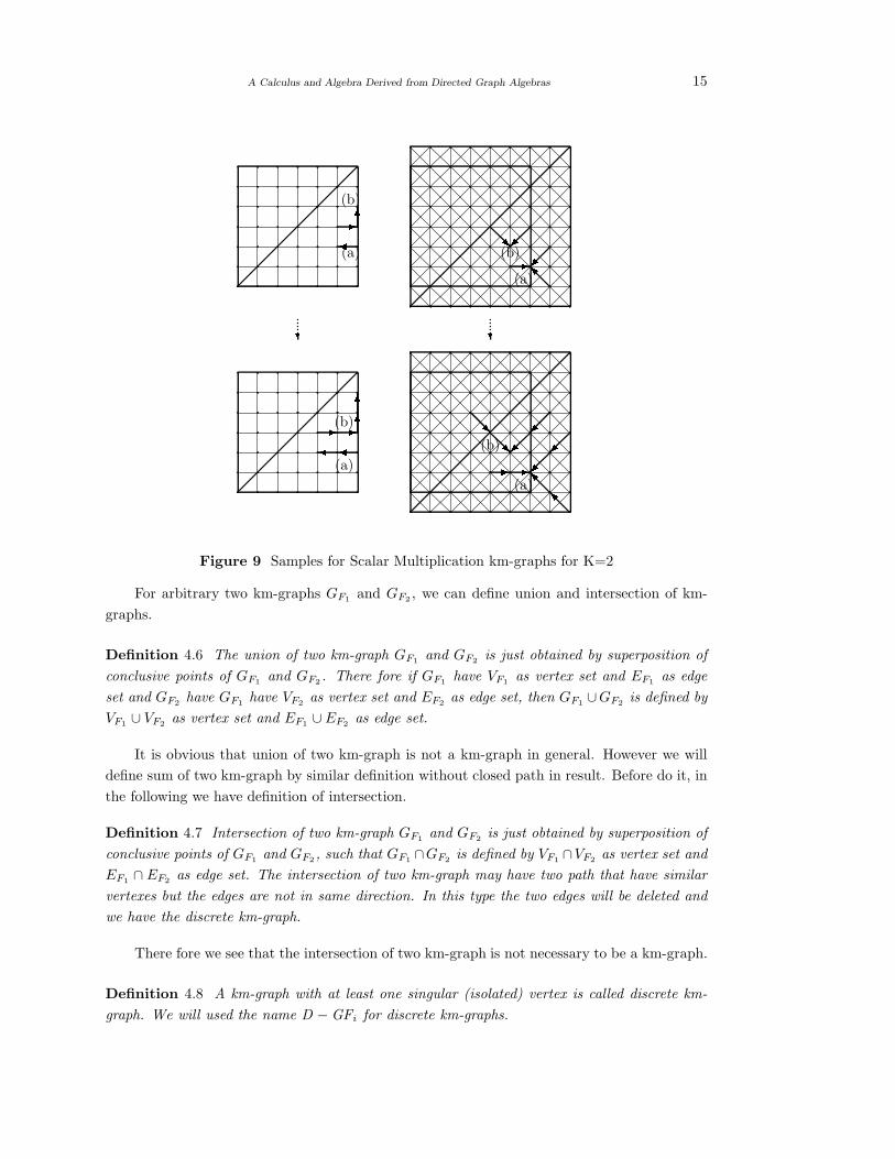
For arbitrary two km-graphs GF1 and GF2 , we can define union and intersection of km-
graphs.
Definition 4.6 The union of two km-graph GF1 and GF2 is just obtained by superposition of
conclusive points of GF1 and GF2 . There fore if GF1 have VF1 as vertex set and EF1 as edge
set and GF2 have GF1 have VF2 as vertex set and EF2 as edge set, then GF1 ∪GF2 is defined by
VF1 ∪ VF2 as vertex set and EF1 ∪ EF2 as edge set.
It is obvious that union of two km-graph is not a km-graph in general. However we will
define sum of two km-graph by similar definition without closed path in result. Before do it, in
the following we have definition of intersection.
Definition 4.7 Intersection of two km-graph GF1 and GF2 is just obtained by superposition of
conclusive points of GF1 and GF2 , such that GF1 ∩GF2 is defined by VF1 ∩VF2 as vertex set and
EF1 ∩ EF2 as edge set. The intersection of two km-graph may have two path that have similar
vertexes but the edges are not in same direction. In this type the two edges will be deleted and
we have the discrete km-graph.
There fore we see that the intersection of two km-graph is not necessary to be a km-graph.
Definition 4.8 A km-graph with at least one singular (isolated) vertex is called discrete km-
graph. We will used the name D − GFi for discrete km-graphs.
16 Kh.Shahbazpour and Mahdihe Nouri- ��--�?6��^o-�?67�^o -�?67�o^ -�?67�^o -�6?7�^o-�?6��^-o�?67�so
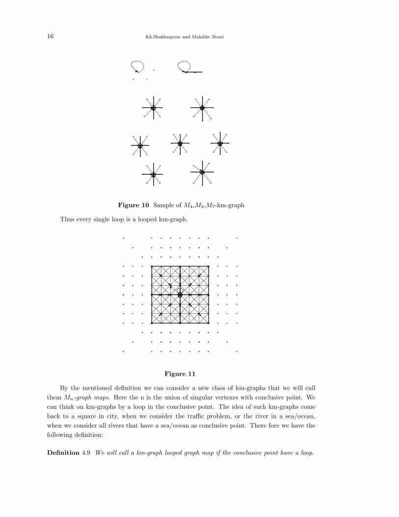
Figure 10 Sample of M4,M3,M7-km-graph
Thus every single loop is a looped km-graph.
R R6R?6?? - - -� � �666 III ���Figure 11
By the mentioned definition we can consider a new class of km-graphs that we will call
them Mn-graph maps. Here the n is the union of singular vertexes with conclusive point. We
can think on km-graphs by a loop in the conclusive point. The idea of such km-graphs come
back to a square in city, when we consider the traffic problem, or the river in a sea/ocean,
when we consider all rivers that have a sea/ocean as conclusive point. There fore we have the
following definition:
Definition 4.9 We will call a km-graph looped graph map if the conclusive point have a loop.
A Calculus and Algebra Derived from Directed Graph Algebras 17
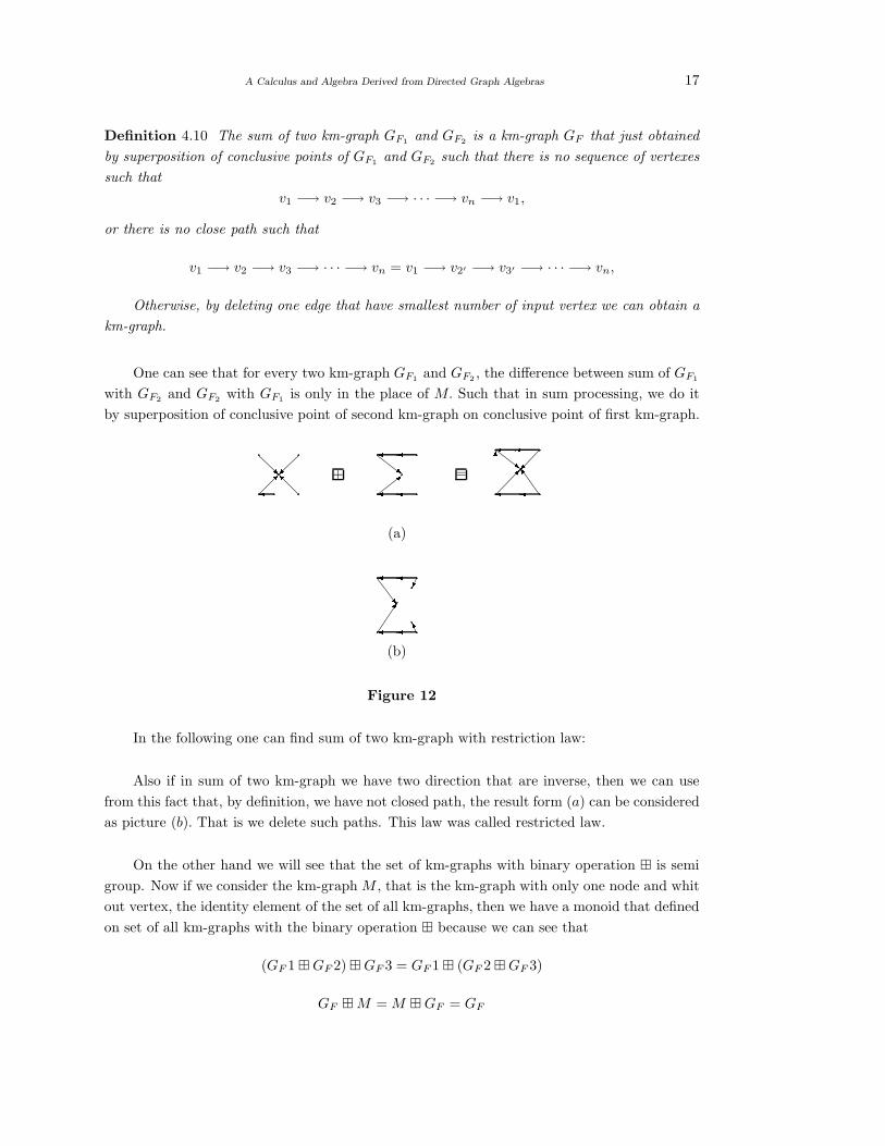
Definition 4.10 The sum of two km-graph GF1 and GF2 is a km-graph GF that just obtained
by superposition of conclusive points of GF1 and GF2 such that there is no sequence of vertexes
such that
v1 −→ v2 −→ v3 −→ · · · −→ vn −→ v1,
or there is no close path such that
v1 −→ v2 −→ v3 −→ · · · −→ vn = v1 −→ v2′ −→ v3′ −→ · · · −→ vn,
Otherwise, by deleting one edge that have smallest number of input vertex we can obtain a
km-graph.
One can see that for every two km-graph GF1 and GF2 , the difference between sum of GF1
with GF2 and GF2 with GF1 is only in the place of M. Such that in sum processing, we do it
by superposition of conclusive point of second km-graph on conclusive point of first km-graph.R�I� +
��~��> =
��6 ���~o(a)��w ���� K(b)
Figure 12
In the following one can find sum of two km-graph with restriction law:
Also if in sum of two km-graph we have two direction that are inverse, then we can use
from this fact that, by definition, we have not closed path, the result form (a) can be considered
as picture (b). That is we delete such paths. This law was called restricted law.
On the other hand we will see that the set of km-graphs with binary operation ⊞ is semi
group. Now if we consider the km-graph M , that is the km-graph with only one node and whit
out vertex, the identity element of the set of all km-graphs, then we have a monoid that defined
on set of all km-graphs with the binary operation ⊞ because we can see that
(GF 1 ⊞ GF 2) ⊞ GF 3 = GF 1 ⊞ (GF 2 ⊞ GF 3)
GF ⊞ M = M ⊞ GF = GF
18 Kh.Shahbazpour and Mahdihe Nouri-?��66- - -???�� + -�?6 =
- - -6???��66 �� -????(a)
66- - -???��-?�??(b)
Figure 13-? -6 6x y
z
t p
M + �6-?�x’
y’z’
t’p’
=
-?-?��6 6x y
M
x’
y’z’M
t’p’
(1. ) (2. ) (3. )
x -? -6 ?6��(b)
(a)
y x’
y’z’
t’ p’
M
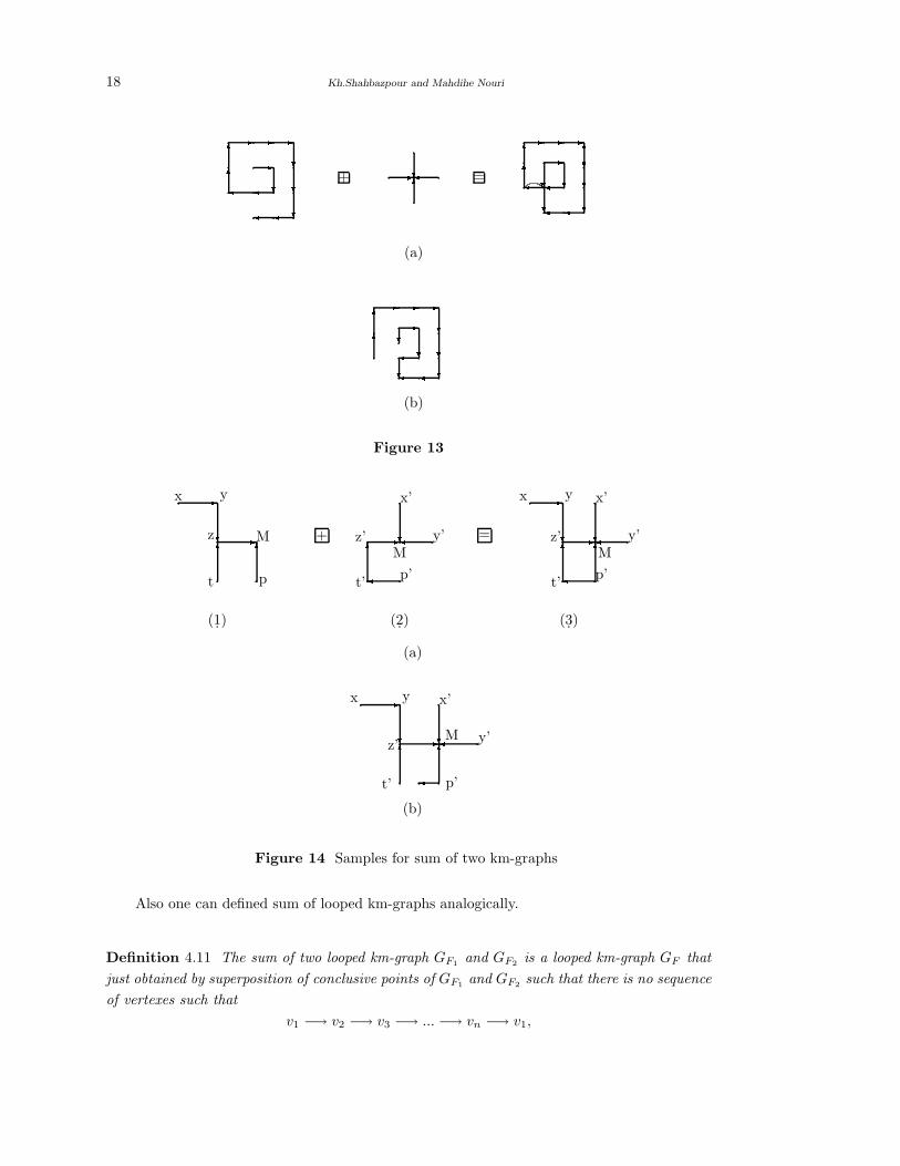
Figure 14 Samples for sum of two km-graphs
Also one can defined sum of looped km-graphs analogically.
Definition 4.11 The sum of two looped km-graph GF1 and GF2 is a looped km-graph GF that
just obtained by superposition of conclusive points of GF1 and GF2 such that there is no sequence
of vertexes such that
v1 −→ v2 −→ v3 −→ ... −→ vn −→ v1,
A Calculus and Algebra Derived from Directed Graph Algebras 19
or there is no close path such that
v1 −→ v2 −→ v3 −→ ... −→ vn = v1 −→ v2′ −→ v3′ −→ ... −→ vn,
Otherwise, by deleting one edge that have smallest number of input vertex we can obtain a
km-graph.
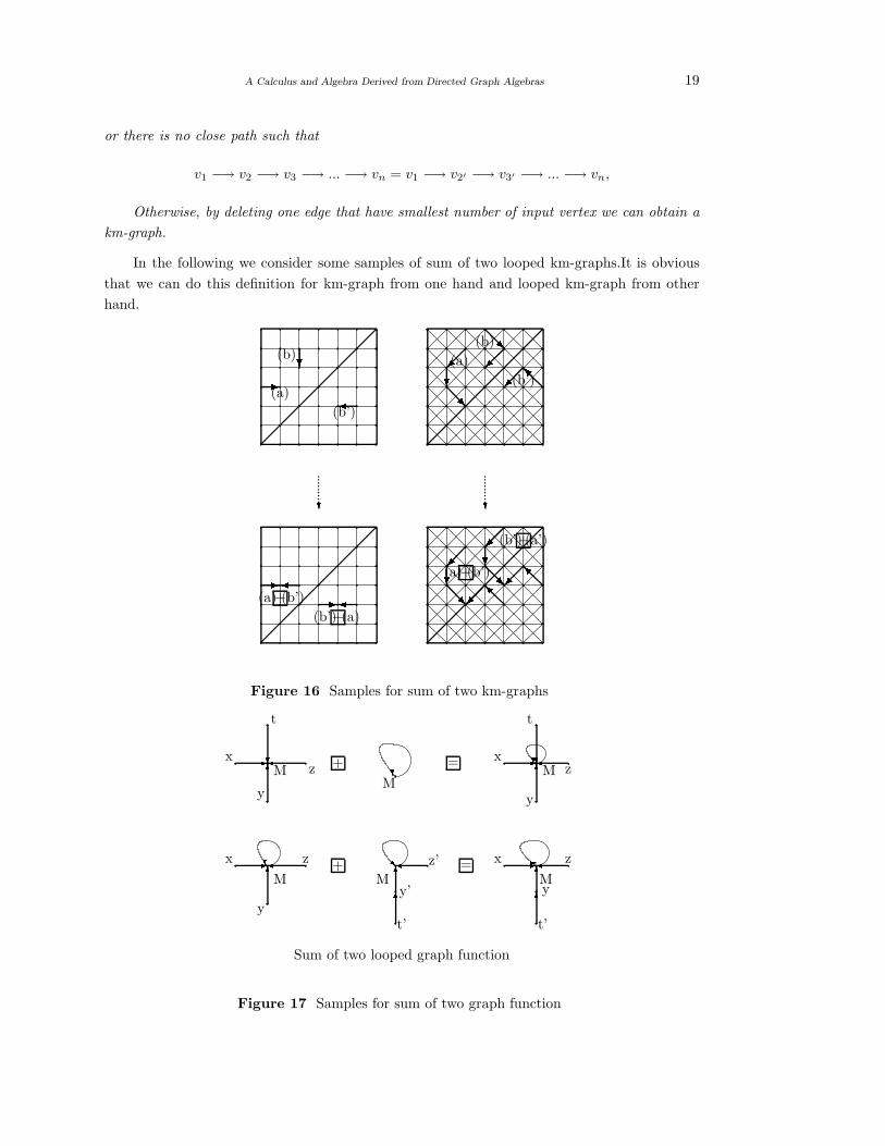
In the following we consider some samples of sum of two looped km-graphs.It is obvious
that we can do this definition for km-graph from one hand and looped km-graph from other
hand. ?- � ?R.........
.........
R? ?
I(a)
(b)
(b’)
(a)
(b)
(b’)
-� -� ?R I?R I(a)+(b’)
(b’)+(a)
(a)+(b’)
(b’)+(a’)
Figure 16 Samples for sum of two km-graphs?6-� + ? = ?6-�?x
y
z
t
MM
Mx
y
z
t
-�6?x
y
z + 66�RM My’
t’
z’ = -�66-M
x
y
z
t’
Sum of two looped graph function
Figure 17 Samples for sum of two graph function
20 Kh.Shahbazpour and Mahdihe Nouri
-�?6�RI + - = -�?6�IR?Figure 18 Samples for sum of two graph function
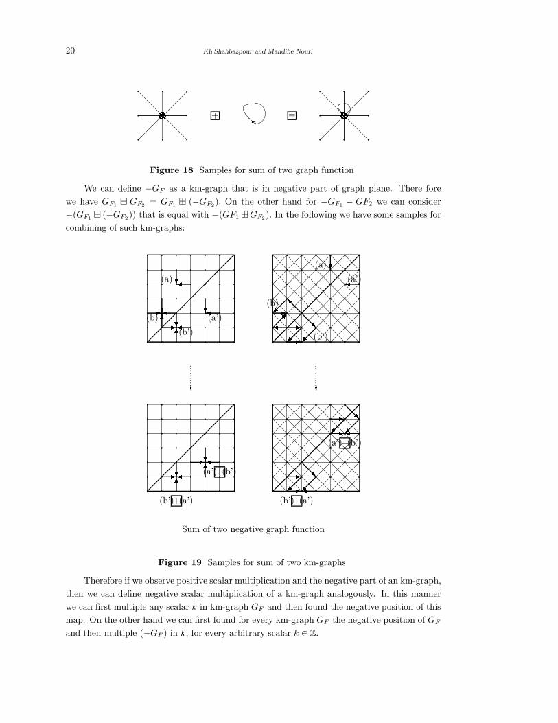
We can define −GF as a km-graph that is in negative part of graph plane. There fore
we have GF1 ⊟ GF2 = GF1 ⊞ (−GF2). On the other hand for −GF1 − GF2 we can consider
−(GF1 ⊞ (−GF2)) that is equal with −(GF1 ⊞ GF2). In the following we have some samples for
combining of such km-graphs:?� ?�?-.........
.........
6�? ?
?-�6(a)
(b)
(b’)
(a’)
? �-�� --I R(a)
(a’)
(b)
(b’)
-?�6 -�?6 R--�R�--(a’)+(b’)
(b’)+(a’) (b’)+(a’)
(a’)+(b’)
Sum of two negative graph function
Figure 19 Samples for sum of two km-graphs
Therefore if we observe positive scalar multiplication and the negative part of an km-graph,
then we can define negative scalar multiplication of a km-graph analogously. In this manner
we can first multiple any scalar k in km-graph GF and then found the negative position of this
map. On the other hand we can first found for every km-graph GF the negative position of GF
and then multiple (−GF ) in k, for every arbitrary scalar k ∈ Z.
A Calculus and Algebra Derived from Directed Graph Algebras 21
4.1 Algebraic Properties of km-Graphs
First of all we will consider associativity and commutativity properties for sum of km-graphs.
Sum of two km-graphs are defined in previous section. The drawing km-graph for sum of GF1
with GF2 and GF2 with GF1 are similar, but are in different place of graph plane. There fore
one can conclude that the sum of two km-graph is approx-commutative. Also one can see that
the approx-associativity property hold for sum of three km-graphs.
On the other hand sum of every km-graph GF1 with km-graph GFM, is GF1 (where GFM
is
the km-graph with only one vertex and no edges). Thus, one can conclude that the class of all
km-graphs considerable as a approx-commutative monoid (the approx-commutative semi-group
with identity element).
On the other hand if we consider the km-graph as objects and the binary operation between
them be the sum of two km-graphs, then can we have a category?
In this direction one can discussed that which properties of categories are satisfies in men-
tioned category and vise verse. It is obvious that by definition of km-graph and drawing them
we have the following lemmas:
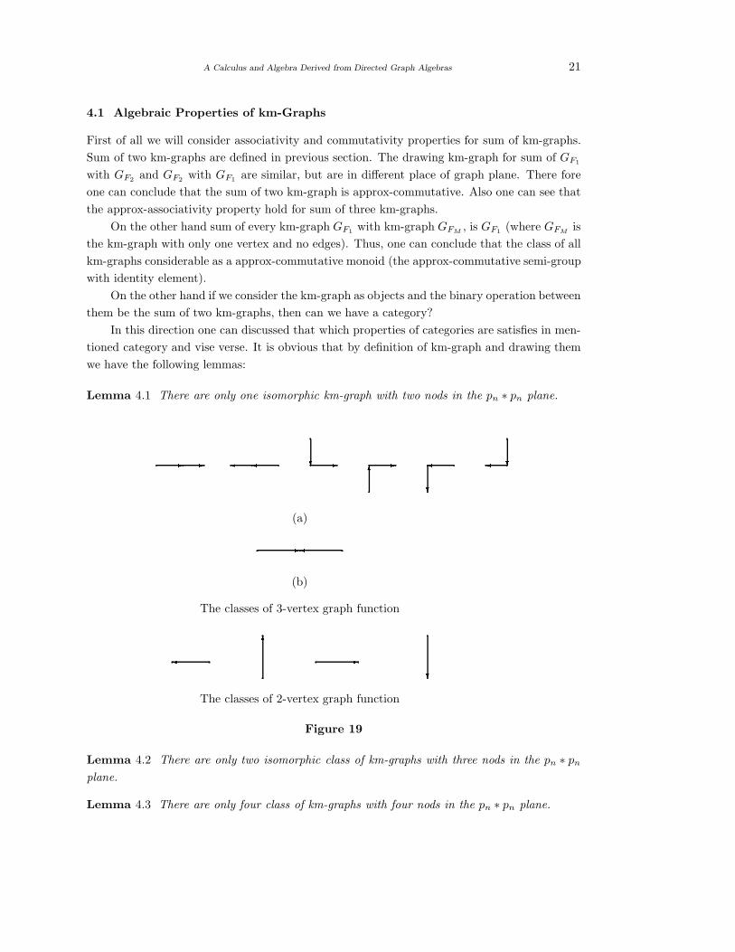
Lemma 4.1 There are only one isomorphic km-graph with two nods in the pn ∗ pn plane.- - �� ?- 6- �? ?�(a)-�
The classes of 3-vertex graph function
(b)
� 6 - ?The classes of 2-vertex graph function
Figure 19
Lemma 4.2 There are only two isomorphic class of km-graphs with three nods in the pn ∗ pn
plane.
Lemma 4.3 There are only four class of km-graphs with four nods in the pn ∗ pn plane.
22 Kh.Shahbazpour and Mahdihe Nouri
4.2 km-Algebras
Definition 4.12 We call an algebra defined on km-graphs a KM − Algebra, if the following
laws holds:
xy ≈ y (1)
yx ≈ ∞ (2)
MM ≈ ∞ (3)
yM ≈ ∞ (4)
My ≈ ∞ (5)
M∞ ≈ ∞ (6)
∞M ≈ ∞ (7)
y∞ ≈ ∞ (8)
∞y ≈ ∞ (9)
y(yM) ≈ yM (10)
M(yM) ≈ MM ≈ ∞ (11)
(xy)z ≈ (xy)(yz) ≈ yz (12)
x1x2x3 · · ·xny ≈ y1y2y3 · · · ymy (13)
Equational theory on km-algebras can be discussed for identities and hyperidentities in
nontrivial terms.
In [1], Baker, McNulty, and Werner give a method, the Shift-Automorphism Theorem, for
showing that certain algebras are INFB. This method is particularly useful in the case of graph
algebras; it is an essential ingredient in the classification in [1] of the FB graph algebras. The
shift-automorphism theorem 4.5 can be used to show that many directed graph algebras are
INFB as well, and we shall use it to obtain several such results in this chapter.
The form of the shift-automorphism theorem that we shall use is Theorem in [1], and it
appears below as our . In an algebra that has an absorbing element ∞, as do all directed
graph algebras, the proper elements are the elements other than ∞. Given a Z−sequence α,
the translates of α are the sequences αi for i ∈ Z, where αi is α shifted i places to the right.
(Thus if i < 0, then we shift to the left, and if i = 0 then we do not shift at all.)
Theorem 4.1(Shift-Automorphism Theorem) Let B be a finite algebra of finite type, with an
absorbing element ∞. Suppose that a sequence α of proper elements of B can be found with
these properties:
(1) in Bz, any fundamental operation f applied to translates of α yields as a value either
a translate of α or a sequence containing ∞;
A Calculus and Algebra Derived from Directed Graph Algebras 23
(2) there are only finitely many equations f(αi1 , · · · , αin(f)) = α(j) in which f is a funda-
mental operation and some argument is a α itself;
(3) there is at least one equation f(αi1 , · · · , αin(f)) = α(1) in which some argument is a
itself, in an entry on which f actually depends,
then B is INFB.
Proof See [23]. 2The general idea of this version of the Shift-Automorphism Theorem, as applied specifically
to a directed graph algebra B, is that we want to use α to create an infinite directed graph
with certain properties. The elements of this directed graph are the translates of α, and the
edges are the natural ones inherited from GB. We pool all sequences that contain ∞ into an
equivalence class, which acts as the ∞ element for resulting infinite directed graph algebra.
Condition (a) of the theorem ensures that this view makes sense. Condition (b) requires there
to be only finitely many edges into and out of α ( and therefore into and out of any α(i));
another way to say this is that there must be an N such that if n ≥ N , then αα(n) and α(n)α
must both contain an occurrence of ∞. (Here α(i)α(j) is understood to be the result of applying
our binary operation coordinate wise to α(i) and α(j).) Condition (c) tells us that there has to
be edge from α(1) to α.
Because the multiplication in our km-algebras has the property that uv is either v or ∞,
if B is a KM-Algebra and α is any sequence of proper elements of B, then it is clear that
condition (a) of the theorem is satisfied; in each coordinate of α, the product will either be the
right-hand operand or ∞. Hence we do not need to mention condition (a) again when dealing
with km-algebra. Note also that if α is an infinite path through GB, as it will be in all of the
cases we consider, then condition (c) must hold.
The original version of the shift automorphism theorem, as formulated in 1989 by Baker,
McNulty, and Werner [1], stated that any shift automorphism algebra is inherently nonfinitely
based. In 2008, McNulty, Szekly, and Willard were able to show every shift automorphism
algebra must be inherently nonfinitely based in the finite sense [16]. It is the contribution of
this author that every shift automorphism variety has countably infinite sub directly irreducible
members.
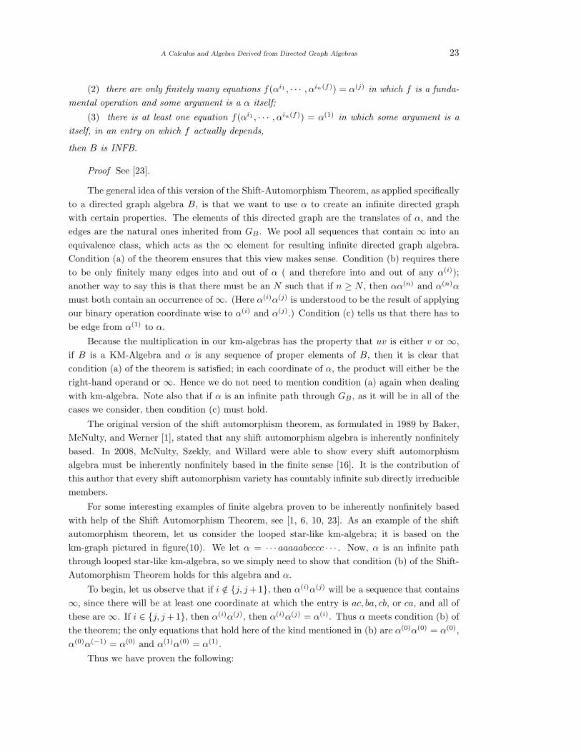
For some interesting examples of finite algebra proven to be inherently nonfinitely based
with help of the Shift Automorphism Theorem, see [1, 6, 10, 23]. As an example of the shift
automorphism theorem, let us consider the looped star-like km-algebra; it is based on the
km-graph pictured in figure(10). We let α = · · · aaaaabcccc · · · . Now, α is an infinite path
through looped star-like km-algebra, so we simply need to show that condition (b) of the Shift-
Automorphism Theorem holds for this algebra and α.
To begin, let us observe that if i /∈ {j, j +1}, then α(i)α(j) will be a sequence that contains
∞, since there will be at least one coordinate at which the entry is ac, ba, cb, or ca, and all of
these are ∞. If i ∈ {j, j +1}, then α(i)α(j), then α(i)α(j) = α(i). Thus α meets condition (b) of
the theorem; the only equations that hold here of the kind mentioned in (b) are α(0)α(0) = α(0),
α(0)α(−1) = α(0) and α(1)α(0) = α(1).
Thus we have proven the following:
24 Kh.Shahbazpour and Mahdihe Nouri
Lemma 4.4 For n ≥ 3 every n-Starlike km-algebra is INFB.
Also for the looped n-starlike km-algebra the above lemma is true. The infinite looped
star-like km-algebra that α yields is pictured in Figure 10.
Note that the same α would have worked even if the km-algebra in question had either
(or both) of the edges (b, a) and (c, b). Thus the km-algebras in Figure 10 give rise to INFB
km-algebras as well.
Also the nullary looped km-algebra (with one vertex and one edges) is just a single looped
element, so is FB. Thus we have now completely classified the looped star-like km-algebras.
To use the Shift-Automorphism Method, consider B, a finite algebra of finite signa-
ture. We will consider the Z−tuple (· · · , b−2, b−1, b0, b1, b2, · · · ) in BZ as a sequence α =
· · · b−2b−1b0b1b2 · · · where each bj is a proper element of B for every j ∈ Z. We define αi as
the ith translate of α, that is, as α shifted ipositions to the right (if i > 0), to the left (if i < 0),
or not at all (if i = 0). Note that the shift by 1 position is an automorphism of BZ. If σ gives
only one infinite orbit, then we can summarize Theorem 4.1 as the following, also found on [1].
Theorem 4.2 Let B be a finite algebra of finite signature with absorbing element 0. Suppose
that a sequence α of proper elements of B can be found with these properties:
(1) in BZ, any fundamental operation F applied translates of α yields as a value either a
translate of α or a sequence containing 0;
(2) there are only finitely many equations (αi0 , · · · , αir−1) = αj in which F is a funda-
mental operation of rank r and some argument is α itself;
(3) there is at least one equation F (αi0 , · · · , αir−1) = α1 in which some argument is α
itself, in an entry on which F actually depends.
We apply Theorems 4.1 and 4.2 to various algebras to show that they are inherently
nonfinitely based.
4.3 Walter’s Looped Directed Graphs
Walter gives the following adapted version of Theorem 4.2.
Theorem 4.3([23]) Let G be a directed graph, and let α be a Z−sequence that is a path of G.
If there is an N such that n > N implies that αn.α and α.αn both contain an occurrence of ∞,
then the graph algebra of G in inherently nonfinitely based.
Now for our km-algebras we have another version of Theorem 4.2.
Theorem 4.4 Let G be a KM- algebra, and α be a Z−sequence that is a path of G. If there is
an N such that n > N implies that αn.α and α.αn both contain an occurrence of ∞, then the
km-algebra G is inherently nonfinitely based.
Proof We will show the connection between Theorems 4.1 and 4.3. Let µ be a km-algebra
and let α be a Z-sequence that is a path through B. We will check the conditions of Theorem
4.1.
A Calculus and Algebra Derived from Directed Graph Algebras 25
The first condition of Theorem 4.1 requires that any fundamental operation applied to any
translate of α results in another translate of α, or a sequence containing ∞. As our operation
is inherited from a graph algebra, the operation. works as follows:
u.v =
v if(u, v) ∈ E
∞ otherwise
Thus for the coordinate wise product of two Z−sequence αj , αk we get
αj , αk
αk
γ whereγisasequencecontaining∞
since the result of applying. Coordinate wise gives either right input or ∞.
The second condition of Theorem 4.1 requires that there be only finitely many proper
equations using the fundamental operation and the translates of α. In terms of our new infinite
km-algebra, this conditions there to only finitely many edge into and out of each αi. This is
equivalent to having the existence of a number N so that for all n > N we have αn.α and α.αn
each contain an occurrence of ∞.
Since α1 is a path through the km-algebra, α1.α0 = α0. To see this, consider a string
· · ·x−3x−2x−1x0x1x2x3 · · · in α1 where each xi is a vertex in the km-graph related to km-
algebra. Then α1 has the same string, just shifted one place rightward. Since α1 gives a path,
we know that must be an edge between xi and xi+1 for i = −1, ...4. Thus the product xi.xi+1
results xi+1. Hence we get the following
α1 : · · ·x−1x0x1x2x3 · · ·
α0 : · · ·x0x1x2x3x4 · · ·
· · · · · · · · · · · · · · · · · · · · ·
α0 : · · ·x0x1x2x3x4 · · ·
This gives the last condition of Theorem 4.1. 2§5. Basic Laws for Directed Mn-km-Graphs
Definition 5.1
M1M1 ≈ ∞ (14)
M1x ≈ ∞ (15)
xM1 ≈ M1 (16)
x∞ ≈ ∞ (17)
∞x ≈ ∞ (18)
26 Kh.Shahbazpour and Mahdihe Nouri
xx ≈ ∞ (19)
xy ≈ y (20)
(xM1)M1 ≈ M1M1 ≈ ∞ (21)
x1x2 · · ·xnM1 ≈ y1y2 · · · ymM1 (22)
For discrete points, MiMj ≈ ∞.
Lemma 5.1 The identity (xM1)M1 ≈ M1(xM1) holds.
Proof (xM1)M1 ≈ by (16), (xM1)(xM1) ≈ by (16) and then ≈ M1(xM1). 2§6. Basic Laws for Directed Looped Mn-km-Graphs
Definition 6.1
M1M1 ≈ M1 (23)
M1x ≈ ∞ (24)
xM1 ≈ M1 (25)
x∞ ≈ ∞ (26)
∞x ≈ ∞ (27)
xx ≈ ∞ (29)
xy ≈ y (30)
(xy)y ≈ yy ≈ ∞ (31)
x1x2 · · ·xnM ≈ y1y2 · · · ymM (32)
For discrete points, MiMj ≈ ∞.
Lemma 6.1 The identity (xy)y ≈ y(xy) holds.
Proof (xy)y ≈ by (29), yy ≈ by (29) and then ≈ y(xy). 2§7. Basic Laws for Looped km-Algebra
Definition 7.1
MM ≈ M (33)
yM ≈ M (34)
A Calculus and Algebra Derived from Directed Graph Algebras 27
My ≈ ∞ (35)
M∞ ≈ ∞ (36)
∞M ≈ ∞ (37)
y(yM) ≈ yM ≈ M (38)
(xy)M ≈ yM ≈ M (39)
(yM)M ≈ MM ≈ ∞ (40)
M(yM) ≈ MM ≈ ∞ (41)
x1x2 · · ·xnM ≈ y1y2 · · · ymM (42)
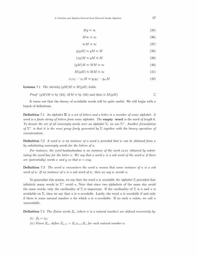
Lemma 7.1 The identity (yM)M ≈ M(yM) holds.
Proof (yM)M ≈ by (34), MM ≈ by (34) and then ≈ M(yM). 2It turns out that the theory of avoidable words will be quite useful. We will begin with a
bunch of definitions.
Definition 7.1 An alphabet Σ is a set of letters and a letter is a member of some alphabet. A
word is a finite string of letters from some alphabet. The empty word is the word of length 0.
To denote the set of all nonempty words over an alphabet Σ, we use Σ+. Another formulation
of Σ+ is that it is the semi group freely generated by Σ together with the binary operation of
concatenation.
Definition 7.2 A word w is an instance of a word u provided that w can be obtained from u
by substituting nonempty words for the letters of u.
For instance, the word baabaabaabaa is an instance of the word xxxx obtained by substi-
tuting the word baa for the letter x. We say that a word u is a sub word of the word w if there
are (potentially) words x and y so that w = xuy.
Definition 7.3 The word w encounters the word u means that some instance of u is a sub
word of w. If no instance of u is a sub word of w, then we say w avoids u.
To generalize this notion, we say that the word u is avoidable the alphabet Σ provided that
infinitely many words in Σ+ avoid u. Note that since two alphabets of the same size avoid
the same words, only the cardinality of Σ is important. If the cardinality of Σ is n and u is
avoidable on Σ, then we say that u is n-avoidable. Lastly, the word u is avoidable if and only
if there is some natural number n for which u is n-avoidable. If no such n exists, we call u
unavoidable.
Definition 7.4 The Zimin words Zn (where n is a natural number) are defined recursively by:
(i) Z0 = x0;
(ii) Given Zn, define Zn+1 = Znxn+1Zn for each natural number n.
28 Kh.Shahbazpour and Mahdihe Nouri
Thus the first three Zimin words are x0, x0x1x0, and x0x1x0x2x0x1x0. If S is a semi group
and w is a word in which the letters of w are regarded as variables, we say w is an isoterm of
S when u and w are identical whenever S |= w ≈ u. See [26] for a development of the theory of
avoidable words.
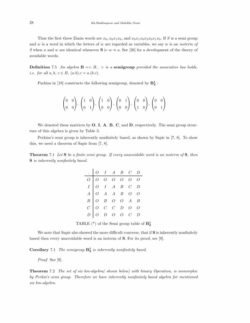
Definition 7.5 An algebra B =< B, . > is a semigroup provided the associative law holds,
i.e. for all a, b, c ∈ B, (a.b).c = a.(b.c).
Parkins in [19] constructs the following semigroup, denoted by B12 :
0 0
0 0
,
1 0
0 1
,
1 0
0 0
,
0 1
0 0
,
0 0
1 0
,
0 0
0 1
We denoted these matrices by O, I, A, B, C, and D, respectively. The semi group struc-
ture of this algebra is given by Table 3.
Perkins’s semi group is inherently nonfinitely based, as shown by Sapir in [7, 8]. To show
this, we need a theorem of Sapir from [7, 8].
Theorem 7.1 Let S be a finite semi group. If every unavoidable word is an isoterm of S, then
S is inherently nonfinitely based.
. O I A B C D
O O O O O O O
I O I A B C D
A O A A B O O
B O B O O A B
C O C C D O O
D O D O O C D
TABLE (*) of the Semi group table of B12
We note that Sapir also showed the more difficult converse, that if S is inherently nonfinitely
based then every unavoidable word is an isoterm of S. For its proof, see [9].
Corollary 7.1 The semigroup B12 is inherently nonfinitely based.
Proof See [9]. 2Theorem 7.2 The set of six km-algebra( shown below) with binary Operation, is isomorphic
by Perkin’s semi group. Therefore we have inherently nonfinitely based algebra for mentioned
six km-algebra.
A Calculus and Algebra Derived from Directed Graph Algebras 29
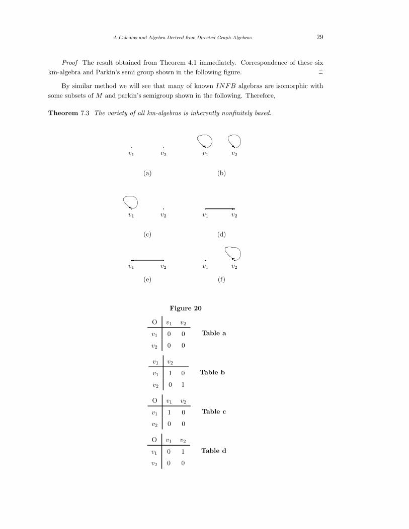
Proof The result obtained from Theorem 4.1 immediately. Correspondence of these six
km-algebra and Parkin’s semi group shown in the following figure. 2By similar method we will see that many of known INFB algebras are isomorphic with
some subsets of M and parkin’s semigroup shown in the following. Therefore,
Theorem 7.3 The variety of all km-algebras is inherently nonfinitely based.- Rv1 v2 v1 v2
(a) (b)- -v1 v2 v1 v2
(c) (d)� -v1 v2 v1 v2
(e) (f)
Figure 20
O v1 v2
v1 0 0
v2 0 0
Table a
v1 v2
v1 1 0
v2 0 1
Table b
O v1 v2
v1 1 0
v2 0 0
Table c
O v1 v2
v1 0 1
v2 0 0
Table d
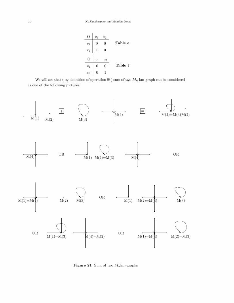
30 Kh.Shahbazpour and Mahdihe Nouri
O v1 v2
v1 0 0
v2 1 0
Table e
O v1 v2
v1 0 0
v2 0 1
Table f
We will see that ( by definition of operation ⊞ ) sum of two Mn km-graph can be considered
as one of the following pictures:
?- + ? -?�6M(1) M(2) M(3)
M(4)= ?-
M(1)=M(3)M(2)
-?6-�M(4)
OR ?- R -?�6M(1) M(2)=M(3) M(4)OR
?6-� RM(1)=M(4) M(2) M(3)
OR ?- -?6� RM(1) M(2)=M(4) M(3)
OR -? ?-�6M(1)=M(3) M(4)=M(2)R OR -�?6 R
M(1)=M(4) M(2)=M(3)
Figure 21 Sum of two Mnkm-graphs
A Calculus and Algebra Derived from Directed Graph Algebras 31
References
[1] Kirby A. Baker, G. F. McNulty, H. Werner, The finitely based varieties of graph algebras,
Acta Scient. Math., 51: 3-15, (1987).
[2] Garrett Birkhoff, On Structure of Abstract Algebras, Proc. Cambridge Philos. Soc., 31
(1935), 433-454.
[3] Wieslaw Dziobiak, On infinite vsubdirectly irreducible algebras in locally finite equational
classes, Algebra Universelis, 13 (1981), No. 3, 393-394.
[4] Samuel Eilenberg, M. P. Schutzenberger, On pseudovarieties, Advances in Math., 19 (1976),
No. 3, 413-418.
[5] E. Hajilarov, An inherently nonfinitely based commutative directoid, Algebra Universelis,
36 (1996), No.4, 431-435.
[6] Keith Kearnes and Ross Willard, Inherently nonfinitely based solvable algebras, Canad.
Math. Bull., 37 (1994), No.4, 514-521.
[7] M. V. Sapir, Inherently nonfinitely based finite semigroups, Mat. Sb. (N.S.), 133 (175)
(1987), no. 2, 154-166.
[8] M. V. Sapir, Problems of Burnside type and the finite basis property in varieties of semi-
groups, Izv. Akad. Nauk SSSR Ser. Mat., 51 (1987), no. 2, 319-340.
[9] Kathryn Hope Scott, A Catalogue of Finite Algebras with Nonfinitely Axiomatizable Equa-
tional theories, Ph.D. Thesis, University of south Carolina, 2007.
[10] Agnes Szendrei, Non-finitely based finite groupoids generating minimal varieties, Acta Sci.
Math. (Szeged), 57 (1993), No. 1-4, 593-600.
[11] W.Kiss, R. Poschel, P.prohle, Subvarieties of varieties generated by graph algebras, Acta
Scient. Math.,54(1-2):57-57,(1990).
[12] Ralph McKenzie, George F. McNulty, Walter F. Taylor, Algebras, Lattices, Varieties. Vol
I, The Wads worth and Brooks/cole Mathematics Series, Wads worth and Brooks/cole
Advanced Books and Software, Monterey, CA, 1987.
[13] Ralph McKenzie,The residual bounds of finite algebras, Internat. J. Algebra Comput., 6
(1996), No.1, 1-28.
[14] Ralph McKenzie, Tarski’s finite basis problem is undecidable, Internat. J. Algebra Com-
put., 6 (1996), No. 1, 49-104.
[15] Georg F. McNulty, Residual finiteness and finite equational bases: undecidable properties
of finite algebras, Lectures on Some Recent Works of Ralph McKenzie and Ross Willard.
[16] Georg F. McNulty, Zoltan Szekely, Ross Willard, Equational complexity of the finite algebra
membership problem, IJAC, 18 (2008), 1283-1319.
[17] J. Jezek, G. F. McNulty, Finite axiomatizablity of congruence rich varieties, Algebra Uni-
verselis, 34 (1995), no.2, 191-213.
[18] A.Kaveh, M.Nouri, Weighted graph products for configuration processing of planer and
space structures, International Journal of Space Structure, Vol.24, Number 1,(2009).
[19] Robert E. Park, Equational classes on non-associative ordered algebras, Ph.D. thesis, Uni-
versity of California, Los Angeles, 1976.
[20] Robert W. Quackenbush, Equational classes generated by finite algebras, Algebra Uni-
verselis, 1 (1971/72), 265-266.
32 Kh.Shahbazpour and Mahdihe Nouri
[21] Kathryn Scott Owens, On Inherently Nonfinitely Based Varieties. Ph.D. Thesis, University
of south Carolina, 2009.
[22] L. Wald, Minimal inherently nonfinitely based varieties of groupoids, Ph.D. thesis, Univer-
sity of California, Los Angeles, 1998.
[23] Brin L.Walter, Finite Equntional Bases for Directed Graph Algebras. Ph.D. Thesis,University
of California, 2002.
[24] Brian L.Walter, The finitely based varieties of looped directed graph algebras, Acta Sci.
Math (Szeged), 72(2006), No.3-4, 421-458.
[25] Emil W. Kiss, R. Poschel, P. Prohle, Subvarieties of varieties generated by graph algebras,
Acta Scient. Math., 54(1-2): 57-75, (1990).
[26] Ross Willard, The finite basis problem, Contributions to General Algebra, 15, Heyn, Kla-
genfurt, 2004, pp. 199-206.
International J.Math. Combin. Vol.3(2015), 33-42
Superior Edge Bimagic Labelling
R.Jagadesh
(Department of Mathematics, Easwari Engineering College, Chennai - 6000 089, India)
J.Baskar Babujee
(Department of Mathematics, MIT Campus, Anna University, Chennai - 600 044, India)
E-mail: jagadesh [email protected], [email protected]
Abstract: A graph G(p, q) is said to be edge bimagic total labeling with two common edge
counts k1 and k2 if there exists a bijection f : V ∪ E → {1, 2, · · · , p + q} such that for each
edge uv ∈ E, f(u) + f(v) + f(e) = k1 or k2. A total edge bimagic graph is called superior
edge bimagic if f(E(G)) = {1, 2, · · · , q}. In this paper we have proved superior edge bimagic
labeling for certain class of graphs arising from graph operations.
Key Words: Graph, magic labeling, bijective function, edge bimagic, superior edge
bimagic labeling.
AMS(2010): 05C78.
§1. Introduction
A labelling of a graph G is an assignment f of labels to either the vertices or the edges or both
subject to certain conditions. Labeled graphs are becoming an increasingly useful family of
mathematical Models from broad range of applications.Graph labelling was first introduced in
the late 1960’s. A useful survey on graph labelling by J.A. Gallian (2013) can be found in [1].
All the graphs considered here are finite, simple and undirected. We follow the notation and
terminology of [2]. In most applications labels are positive (or nonnegative) integers, though in
general real numbers could be used.
A (p, q)-graph G = (V, E) with p vertices and q edges is called total edge magic if there
is a bijection f : V ∪ E → {1, 2, · · · , p + q} such that there exists a constant k for any edge
uv in E, f(u) + f(uv) + f(v) = k. The original concept of total edge-magic graph is due to
Kotzig and Rosa [3]. They called it magic graph. A total edge-magic graph is called a superior
edge-magic if f(E(G)) = {1, 2, · · · , q}.It becomes interesting when we arrive with magic type labeling summing to exactly two
distinct constants say k1 or k2. Edge bimagic total labeling was introduced by J. Baskar Babujee
[6]and studied in [7] as (1, 1) edge bimagic labeling. A graph G(p, q) with p vertices and q edges
is called total edge bimagic if there exists a bijection f : V ∪ E → {1, 2, · · · , p + q} such that
1Received December 5, 2014, Accepted August 7, 2015.
34 R.Jagadesh and J.Baskar Babujee
for any edge uv ∈ E, we have two constants k1 and k2 with f(u) + f(v) + f(uv) = k1 or k2. A
total edge-bimagic graph is called superior edge bimagic if f(E(G)) = {1, 2, · · · , q}. Superior
edge bimagic labelling was introduced and studied in [8].
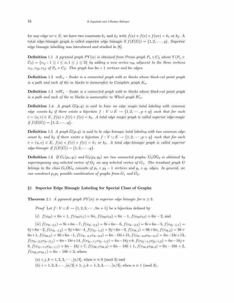
Definition 1.1 A pyramid graph PY (n) is obtained from Prism graph Pn ×C3 whose V (Pn ×C3) = {vij : 1 ≤ i ≤ n, 1 ≤ j ≤ 3} by adding a new vertex v00 adjacent to the three vertices
v11, v12, v13 of Pn × C3. This graph has 3n + 1 vertices and 6n edges.
Definition 1.2 mKn - Snake is a connected graph with m blocks whose block-cut point graph
is a path and each of the m blocks is isomorphic to Complete graph Kn.
Definition 1.3 mWn - Snake is a connected graph with m blocks whose block-cut point graph
is a path and each of the m blocks is isomorphic to Wheel graph Wn.
Definition 1.4 A graph G(p, q) is said to have an edge magic total labeling with common
edge counts k0 if there exists a bijection f : V ∪ E → {1, 2, · · · , p + q} such that for each
e = (u, v) ∈ E, f(u)+ f(v)+ f(e) = k0. A total edge magic graph is called superior edge-magic
if f(E(G)) = {1, 2, · · · , q}.
Definition 1.5 A graph G(p, q) is said to be edge bimagic total labeling with two common edge
count k1 and k2 if there exists a bijection f : V ∪ E → {1, 2, · · · , p + q} such that for each
e = (u, v) ∈ E, f(u) + f(v) + f(e) = k1 or k2. A total edge-bimagic graph is called superior
edge-bimagic if f(E(G)) = {1, 2, · · · , q}.
Definition 1.6 If G1(p1, q1) and G2(p2, q2) are two connected graphs, G1OG2 is obtained by
superimposing any selected vertex of G2 on any selected vertex of G1. The resultant graph G
belongs to the class G1OG2 consists of p1 + p2 − 1 vertices and q1 + q2 edges. In general, we
can construct p1p2 possible combination of graphs from G1 and G2.
§2. Superior Edge Bimagic Labeling for Special Class of Graphs
Theorem 2.1 A pyramid graph PY (n) is superior edge bimagic for n ≥ 3.
Proof Let f : V ∪ E → {1, 2, 3, · · · , 9n + 1} be a bijection defined by
(i) f(v00) = 6n + 1, f(v00v11) = 6n, f(v00v12) = 6n − 1, f(v00v13) = 6n − 2, and
(ii) f(v3i−2,1) = 9i+6n−7, f(v3i−2,2) = 9i+6n−6, f(v3i−2,3) = 9i+6n−5, f(v3j−1,1) =
9j+6n−2, f(v3j−1,2) = 9j+6n−4, f(v3j−1,3) = 9j+6n−3, f(v3k,1) = 9k+6n, f(v3k,2) = 9k+
6n+1, f(v3k,3) = 9k+6n−1, f(v3i−2,1v3i−2,2) = 6n−18i+15, f(v3i−2,2v3i−2,3) = 6n−18i+13,
f(v3i−2,3v3i−2,1) = 6n−18i+14, f(v3j−1,1v3j−1,2) = 6n−18j+8, f(v3j−1,2v3j−1,3) = 6n−18j+
9, f(v3j−1,3v3j−1,1) = 6n− 18j + 7, f(v3k,1v3k,2) = 6n− 18k + 1, f(v3k,2v3k,3) = 6n− 18k + 2,
f(v3k,3v3k,1) = 6n − 18k + 3, where
(a) i, j, k = 1, 2, 3, · · · , [n/3], when n ≡ 0 (mod 3) and
(b) i = 1, 2, 3, · · · , [n/3] + 1; j, k = 1, 2, 3, · · · , [n/3], when n ≡ 1 (mod 3),
Superior Edge Bimagic Labelling 35
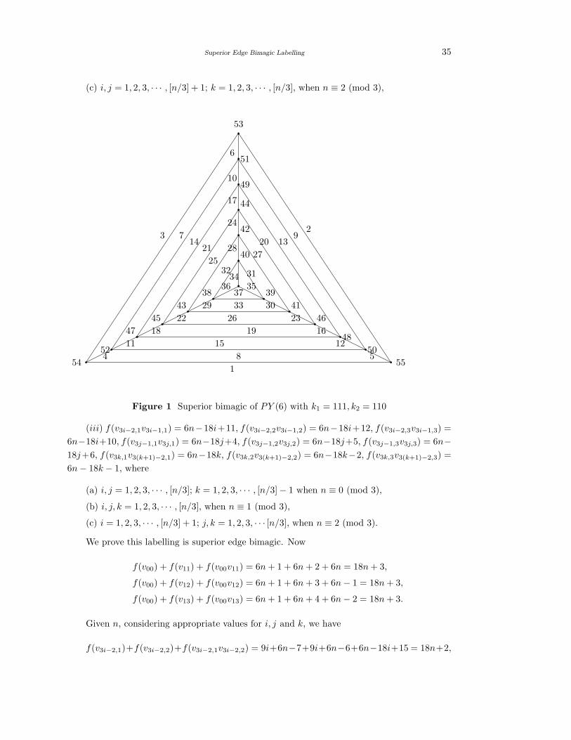
(c) i, j = 1, 2, 3, · · · , [n/3] + 1; k = 1, 2, 3, · · · , [n/3], when n ≡ 2 (mod 3),
53
54 55
50
51
52
48
49
47
46
44
45
41
42
40
37 39
43
38
3 714
21
2532
29
1320
27
31
1
8
15
19
26
33
6
10
17
24
28
34
4
11
18
22
29
36
5
12
16
23
30
35
Figure 1 Superior bimagic of PY (6) with k1 = 111, k2 = 110
(iii) f(v3i−2,1v3i−1,1) = 6n−18i+11, f(v3i−2,2v3i−1,2) = 6n−18i+12, f(v3i−2,3v3i−1,3) =
6n−18i+10, f(v3j−1,1v3j,1) = 6n−18j+4, f(v3j−1,2v3j,2) = 6n−18j+5, f(v3j−1,3v3j,3) = 6n−18j+6, f(v3k,1v3(k+1)−2,1) = 6n−18k, f(v3k,2v3(k+1)−2,2) = 6n−18k−2, f(v3k,3v3(k+1)−2,3) =
6n − 18k − 1, where
(a) i, j = 1, 2, 3, · · · , [n/3]; k = 1, 2, 3, · · · , [n/3]− 1 when n ≡ 0 (mod 3),
(b) i, j, k = 1, 2, 3, · · · , [n/3], when n ≡ 1 (mod 3),
(c) i = 1, 2, 3, · · · , [n/3] + 1; j, k = 1, 2, 3, · · · [n/3], when n ≡ 2 (mod 3).
We prove this labelling is superior edge bimagic. Now
f(v00) + f(v11) + f(v00v11) = 6n + 1 + 6n + 2 + 6n = 18n + 3,
f(v00) + f(v12) + f(v00v12) = 6n + 1 + 6n + 3 + 6n − 1 = 18n + 3,
f(v00) + f(v13) + f(v00v13) = 6n + 1 + 6n + 4 + 6n − 2 = 18n + 3.
Given n, considering appropriate values for i, j and k, we have
f(v3i−2,1)+f(v3i−2,2)+f(v3i−2,1v3i−2,2) = 9i+6n−7+9i+6n−6+6n−18i+15 = 18n+2,
36 R.Jagadesh and J.Baskar Babujee
f(v3i−2,2)+f(v3i−2,3)+f(v3i−2,2v3i−2,3) = 9i+6n−6+9i+6n−5+6n−18i+13 = 18n+2,
f(v3i−2,3)+f(v3i−2,1)+f(v3i−2,3v3i−2,1) = 9i+6n−5+9i+6n−7+6n−18i+14 = 18n+2,
f(v3j−1,1)+f(v3j−1,2)+f(v3j−1,1v3j−1,2) = 9j+6n−2+9j+6n−4+6n−18j+8 = 18n+2,
f(v3k,1) + f(v3k,2) + f(v3k,1v3k,2) = 9k + 6n + 9k + 6n + 1 + 6n − 18k + 1 = 18n + 2.
Also for the remaining any edge uv, the sums f(u) + f(v) + f(uv) = 18n + 2. Hence the
graph PY (n) admits superior edge bimagic labelling. 2The superior edge bimagic labelling of PY (6) shown in the Figure 1.
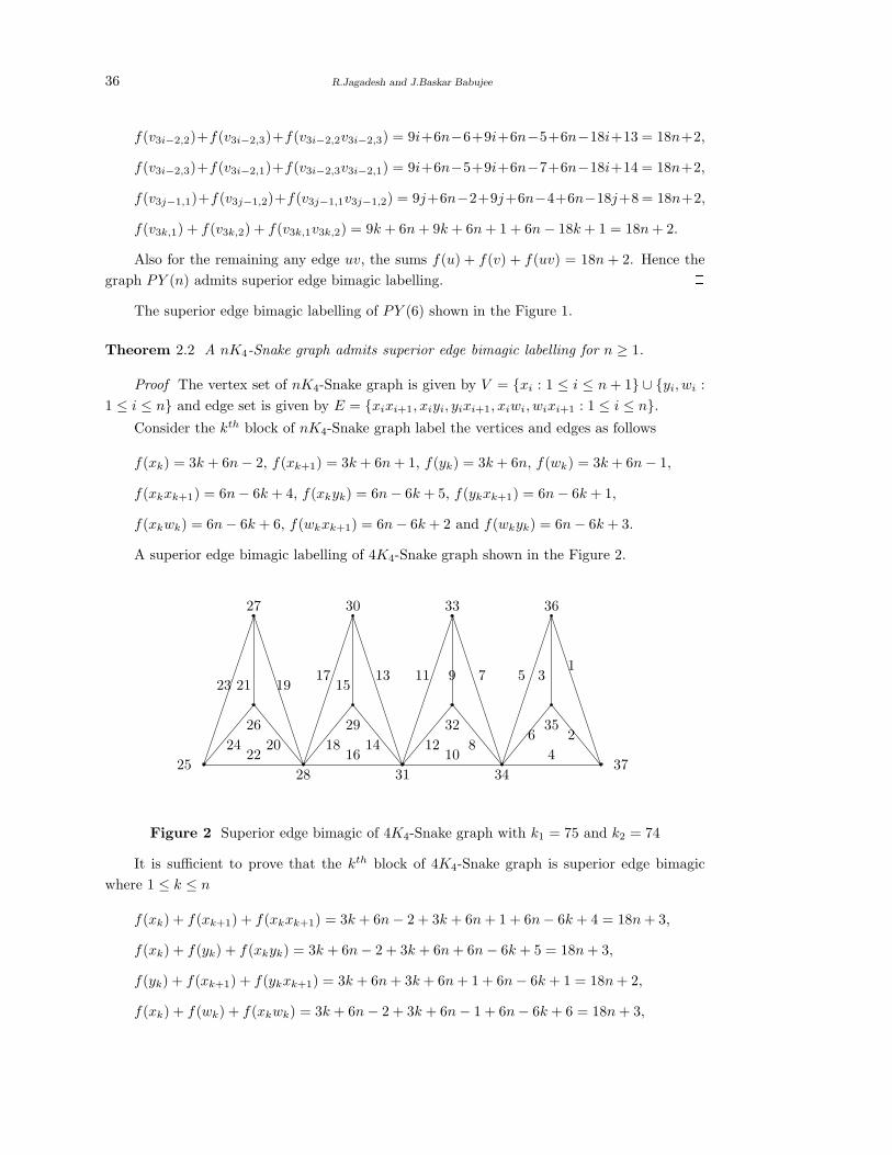
Theorem 2.2 A nK4-Snake graph admits superior edge bimagic labelling for n ≥ 1.
Proof The vertex set of nK4-Snake graph is given by V = {xi : 1 ≤ i ≤ n + 1} ∪ {yi, wi :
1 ≤ i ≤ n} and edge set is given by E = {xixi+1, xiyi, yixi+1, xiwi, wixi+1 : 1 ≤ i ≤ n}.Consider the kth block of nK4-Snake graph label the vertices and edges as follows
f(xk) = 3k + 6n − 2, f(xk+1) = 3k + 6n + 1, f(yk) = 3k + 6n, f(wk) = 3k + 6n − 1,
f(xkxk+1) = 6n− 6k + 4, f(xkyk) = 6n − 6k + 5, f(ykxk+1) = 6n − 6k + 1,
f(xkwk) = 6n − 6k + 6, f(wkxk+1) = 6n − 6k + 2 and f(wkyk) = 6n − 6k + 3.
A superior edge bimagic labelling of 4K4-Snake graph shown in the Figure 2.
2522
28
16
31
10
34
437
27 30 33 36
26 29 32 35
21 159 3
24 18 126
20 14 82
23 1917 13 11 7 5
1
Figure 2 Superior edge bimagic of 4K4-Snake graph with k1 = 75 and k2 = 74
It is sufficient to prove that the kth block of 4K4-Snake graph is superior edge bimagic
where 1 ≤ k ≤ n
f(xk) + f(xk+1) + f(xkxk+1) = 3k + 6n − 2 + 3k + 6n + 1 + 6n− 6k + 4 = 18n + 3,
f(xk) + f(yk) + f(xkyk) = 3k + 6n− 2 + 3k + 6n + 6n − 6k + 5 = 18n + 3,
f(yk) + f(xk+1) + f(ykxk+1) = 3k + 6n + 3k + 6n + 1 + 6n − 6k + 1 = 18n + 2,
f(xk) + f(wk) + f(xkwk) = 3k + 6n − 2 + 3k + 6n − 1 + 6n− 6k + 6 = 18n + 3,
Superior Edge Bimagic Labelling 37
f(wk) + f(xk+1) + f(wkxk+1) = 3k + 6n − 1 + 3k + 6n + 1 + 6n− 6k + 2 = 18n + 2,
f(wk) + f(yk) + f(wkyk) = 3k + 6n− 1 + 3k + 6n + 6n − 6k + 3 = 18n + 2.
Therefore for any edge uv, f(u)+ f(v) + f(uv) yields either 18n+ 3 or 18n+ 2. Hence the
nK4-Snake graph admits superior edge bimagic labelling. 2Theorem 2.3 A nW4-Snake graph admits superior edge bimagic labelling.
Proof The vertex set of nW4 is given by V = {xi : 1 ≤ i ≤ n + 1} ∪ {yi, zi, wi : 1 ≤ i ≤ n}and edge set is given by E = {xiyi, xizi, xiwi, zixi+1, yixi+1, wixi+1 : 1 ≤ i ≤ n}.
Consider the kth block of nW4 and label the vertices and edges as follows
f(xk) = 4k + 8n − 3, f(yk) = 4k + 8n − 1, f(xk+1) = 4k + 8n + 1,
f(zk) = 4k + 8n − 2, f(wk) = 4k + 8n, f(xkyk) = 8n − 8k + 7,
f(ykxk+1) = 8n − 8k + 2, f(xkzk) = 8n − 8k + 8, f(xkwk) = 8n− 8k + 5,
f(zkxk+1) = 8n − 8k + 4, f(wkxk+1) = 8n − 8k + 1,
f(zkyk) = 8n − 8k + 6, and f(ykwk) = 8n − 8k + 3.
It is sufficient to prove that the kth block of nW4 is superior edge bimagic where 1 ≤ k ≤ n
f(xk) + f(yk) + f(xkyk) = 4k + 8n− 3 + 4k + 8n − 1 + 8n − 8k + 7 = 24n + 3,
f(yk) + f(xk+1) + f(ykxk+1) = 4k + 8n − 1 + 4k + 8n + 1 + 8n − 8k + 2 = 24n + 2.
Similarly for any remaining edge uv, f(u)+ f(v)+ f(uv) equals 24n + 3 or 24n + 2. Hence
the graph nW4 admits superior edge bimagic labelling for n ≥ 1. 2Theorem 2.4 There exist a graph from the class PnoK1,m that admits superior edge magic
labeling if n is odd and superior edge bimagic labelling if n is even.
Proof Consider the path Pn with vertex set {x1, x2, · · · , xn} and edge set {xixi+1; 1 ≤ i ≤n − 1}. Let K1,m have vertex set {y1, y2, · · · , ym+1} and edge set {y1yj ; 2 ≤ j ≤ m + 1}.
Let G be a one of the graph from the class PnOK1,m where we superimpose on the vertex
say y1 of K1,m on the selected vertex xn in Pn. The vertex set and edge set of graph G is given
by V = {xi, yj; 1 ≤ i ≤ n, 2 ≤ j ≤ m+1} and E = E1∪E2, where E1 = {xixi+1; 1 ≤ i ≤ n−1}and E2 = {xnyj; 2 ≤ j ≤ m − 1}.
Case 1. n is odd.
Let f : V ∪ E → {1, 2, 3, · · · , 2m + 2n − 1} be the bijective function defined by
f(xi) =
(4m + 4n − 1 − i)/2; i = 1, 3, · · · , n
(4m + 3n − 1 − i)/2; i = 2, 4, · · · , n − 1,
f(yj) = (2m + n + 1 − j); 2 ≤ j ≤ m + 1,
f(xixi+1) = i; 1 ≤ i ≤ n − 1,
38 R.Jagadesh and J.Baskar Babujee
f(xnyj) = (n − 2 + j); 2 ≤ j ≤ m + 1.
For any edge xixi+1 in E1,
f(xi) + f(xi+1) + f(xixi+1) =4m + 4n − 1 − i + 4m + 3n − 1 − i − 1 + 2i
2
=8m + 7n − 3
2= k.
For any edge xnyj in E2,
f(xn) + f(yj) + f(xnyj) =4m + 4n − 1 − n + 4m + 2n + 2 − 2j + 2n − 4 + 2j
2
=8m + 7n − 3
2= k.
Hence the graph G from the class PnOK1,m admits superior edge magic labeling if n is
odd.
Case 2. n is even.
Let f : V ∪ E → {1, 2, 3, · · · , 2m + 2n − 1} be the bijective function defined by
f(xi) =
(4m + 4n − 1 − i)/2; i = 1, 3, · · · , n − 1
(4m + 3n − i)/2; i = 2, 4, . . . , n,
f(yj) = (2m + n + 1 − j); 2 ≤ j ≤ m + 1,
f(xixi+1) = i; 1 ≤ i ≤ n − 1,
f(xnyj) = (n − 2 + j); 2 ≤ j ≤ m + 1.
For any edge xixi+1 in E1,
f(xi) + f(xi+1) + f(xixi+1) =4m + 4n − 1 − i + 4m + 3n− i − 1 + 2i
2
=8m + 7n − 2
2= k1.
For any edge xnyj in E2,
f(xn) + f(yj) + f(xnyj) =4m + 3n − n + 4m + 2n + 2 − 2j + 2n− 4 + 2j
2
=8m + 6n − 2
2= k2.
Hence the graph G from the class PnOK1,m admits superior edge bimagic labeling if n is
even. 2§3. Superior Edge Bimagic Labeling for Some General Graphs
Theorem 3.1 A complete graph Kn (n ≥ 6) is not superior edge bimagic.
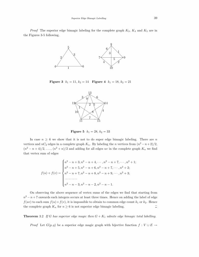
Superior Edge Bimagic Labelling 39
Proof The superior edge bimagic labeling for the complete graph K3, K4 and K5 are in
the Figures 3-5 following.
5
1
2
4 6
37
8
9
10
1
2
3
54
6
Figure 3 k1 = 11, k2 = 14 Figure 4 k1 = 18, k2 = 21
11
12
13
14
15
3 6
4
7
10
2 5
9
1
8
Figure 5 k1 = 28, k2 = 33
In case n ≥ 6 we show that it is not to do super edge bimagic labeling. There are n
vertices and nC2 edges in a complete graph Kn. By labeling the n vertices from (n2−n+2)/2,
(n2 − n + 4)/2, . . . , (n2 + n)/2 and adding for all edges uv in the complete graph Kn we find
that vertex sum of edges
f(u) + f(v) =
n2 − n + 3, n2 − n + 4, · · · , n2 − n + 7, · · · , n2 + 1;
n2 − n + 5, n2 − n + 6, n2 − n + 7, · · · , n2 + 2;
n2 − n + 7, n2 − n + 8, n2 − n + 9, · · · , n2 + 3;
· · · · · · · · ·n2 − n − 3, n2 − n − 2, n2 − n − 1.
On observing the above sequence of vertex sums of the edges we find that starting from
n2 −n + 7 onwards each integers occurs at least three times. Hence on adding the label of edge
f(uv) to each sum f(u)+f(v), it is impossible to obtain to common edge count k1 or k2. Hence
the complete graph Kn for n ≥ 6 is not superior edge bimagic labeling. 2Theorem 3.2 If G has superior edge magic then G + K1 admits edge bimagic total labelling.
Proof Let G(p, q) be a superior edge magic graph with bijective function f : V ∪ E →
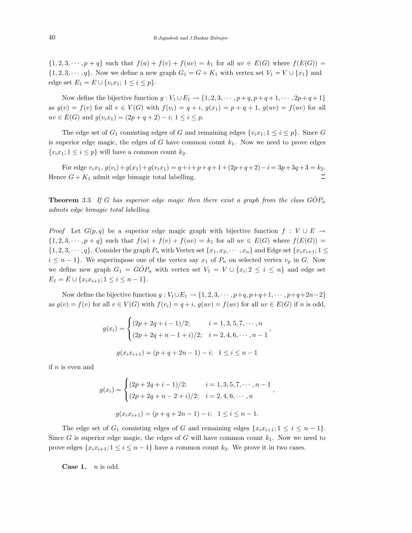
40 R.Jagadesh and J.Baskar Babujee
{1, 2, 3, · · · , p + q} such that f(u) + f(v) + f(uv) = k1 for all uv ∈ E(G) where f(E(G)) =
{1, 2, 3, · · · , q}. Now we define a new graph G1 = G + K1 with vertex set V1 = V ∪ {x1} and
edge set E1 = E ∪ {vix1; 1 ≤ i ≤ p}.
Now define the bijective function g : V1 ∪E1 → {1, 2, 3, · · · , p+ q, p+ q +1, · · · , 2p+ q +1}as g(v) = f(v) for all v ∈ V (G) with f(vi) = q + i, g(x1) = p + q + 1, g(uv) = f(uv) for all
uv ∈ E(G) and g(vix1) = (2p + q + 2) − i; 1 ≤ i ≤ p.
The edge set of G1 consisting edges of G and remaining edges {vix1; 1 ≤ i ≤ p}. Since G
is superior edge magic, the edges of G have common count k1. Now we need to prove edges
{vix1; 1 ≤ i ≤ p} will have a common count k2.
For edge vix1, g(vi)+g(x1)+g(vix1) = q+ i+p+q+1+(2p+q+2)− i = 3p+3q+3 = k2.
Hence G + K1 admit edge bimagic total labelling. 2Theorem 3.3 If G has superior edge magic then there exist a graph from the class GOPn
admits edge bimagic total labelling.
Proof Let G(p, q) be a superior edge magic graph with bijective function f : V ∪ E →{1, 2, 3, · · · , p + q} such that f(u) + f(v) + f(uv) = k1 for all uv ∈ E(G) where f(E(G)) =
{1, 2, 3, · · · , q}. Consider the graph Pn with Vertex set {x1, x2, · · · , xn} and Edge set {xixi+1; 1 ≤i ≤ n − 1}. We superimpose one of the vertex say x1 of Pn on selected vertex vp in G. Now
we define new graph G1 = GOPn with vertex set V1 = V ∪ {xi; 2 ≤ i ≤ n} and edge set
E1 = E ∪ {xixi+1; 1 ≤ i ≤ n − 1}.
Now define the bijective function g : V1∪E1 → {1, 2, 3, · · · , p+q, p+q+1, · · · , p+q+2n−2}as g(v) = f(v) for all v ∈ V (G) with f(vi) = q + i, g(uv) = f(uv) for all uv ∈ E(G) if n is odd,
g(xi) =
(2p + 2q + i − 1)/2; i = 1, 3, 5, 7, · · · , n
(2p + 2q + n − 1 + i)/2; i = 2, 4, 6, · · · , n − 1,
g(xixi+1) = (p + q + 2n− 1) − i; 1 ≤ i ≤ n − 1
if n is even and
g(xi) =
(2p + 2q + i − 1)/2; i = 1, 3, 5, 7, · · · , n − 1
(2p + 2q + n − 2 + i)/2; i = 2, 4, 6, · · · , n,
g(xixi+1) = (p + q + 2n − 1) − i; 1 ≤ i ≤ n − 1.
The edge set of G1 consisting edges of G and remaining edges {xixi+1; 1 ≤ i ≤ n − 1}.Since G is superior edge magic, the edges of G will have common count k1. Now we need to
prove edges {xixi+1; 1 ≤ i ≤ n − 1} have a common count k2. We prove it in two cases.
Case 1. n is odd.
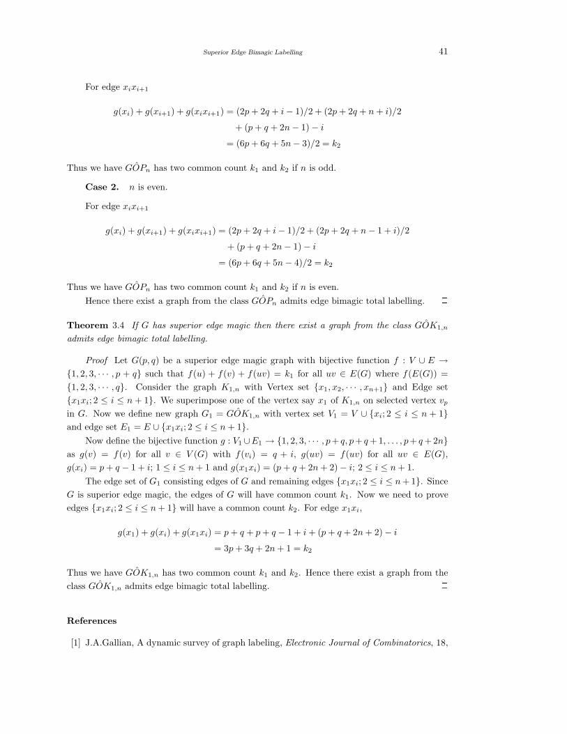
Superior Edge Bimagic Labelling 41
For edge xixi+1
g(xi) + g(xi+1) + g(xixi+1) = (2p + 2q + i − 1)/2 + (2p + 2q + n + i)/2
+ (p + q + 2n − 1) − i
= (6p + 6q + 5n− 3)/2 = k2
Thus we have GOPn has two common count k1 and k2 if n is odd.
Case 2. n is even.
For edge xixi+1
g(xi) + g(xi+1) + g(xixi+1) = (2p + 2q + i − 1)/2 + (2p + 2q + n − 1 + i)/2
+ (p + q + 2n − 1) − i
= (6p + 6q + 5n − 4)/2 = k2
Thus we have GOPn has two common count k1 and k2 if n is even.
Hence there exist a graph from the class GOPn admits edge bimagic total labelling. 2Theorem 3.4 If G has superior edge magic then there exist a graph from the class GOK1,n
admits edge bimagic total labelling.
Proof Let G(p, q) be a superior edge magic graph with bijective function f : V ∪ E →{1, 2, 3, · · · , p + q} such that f(u) + f(v) + f(uv) = k1 for all uv ∈ E(G) where f(E(G)) =
{1, 2, 3, · · · , q}. Consider the graph K1,n with Vertex set {x1, x2, · · · , xn+1} and Edge set
{x1xi; 2 ≤ i ≤ n + 1}. We superimpose one of the vertex say x1 of K1,n on selected vertex vp
in G. Now we define new graph G1 = GOK1,n with vertex set V1 = V ∪ {xi; 2 ≤ i ≤ n + 1}and edge set E1 = E ∪ {x1xi; 2 ≤ i ≤ n + 1}.
Now define the bijective function g : V1 ∪E1 → {1, 2, 3, · · · , p+ q, p+ q +1, . . . , p+ q +2n}as g(v) = f(v) for all v ∈ V (G) with f(vi) = q + i, g(uv) = f(uv) for all uv ∈ E(G),
g(xi) = p + q − 1 + i; 1 ≤ i ≤ n + 1 and g(x1xi) = (p + q + 2n + 2) − i; 2 ≤ i ≤ n + 1.
The edge set of G1 consisting edges of G and remaining edges {x1xi; 2 ≤ i ≤ n + 1}. Since
G is superior edge magic, the edges of G will have common count k1. Now we need to prove
edges {x1xi; 2 ≤ i ≤ n + 1} will have a common count k2. For edge x1xi,
g(x1) + g(xi) + g(x1xi) = p + q + p + q − 1 + i + (p + q + 2n + 2) − i
= 3p + 3q + 2n + 1 = k2
Thus we have GOK1,n has two common count k1 and k2. Hence there exist a graph from the
class GOK1,n admits edge bimagic total labelling. 2References
[1] J.A.Gallian, A dynamic survey of graph labeling, Electronic Journal of Combinatorics, 18,
42 R.Jagadesh and J.Baskar Babujee
# DS6, (2011).
[2] N.Hartsfield and G. Ringel, Pearls in Graph Theory, Academic Press, San Diego, 1990.
[3] A.Kotzig and A. Rosa, Magic valuations of finite graphs, Canada Math. Bull., Vol. 13,
1970, 451-461.
[4] F.Harary, Graph Theory, Addison Wesley, Reading, Massachusetts, 1969.
[5] W.D.Wallis, Magic Graphs, Birkhauser, Basel 2001.
[6] J.Baskar Babujee, Bimagic labeling in path graphs, The Mathematics Education, Volume
38, No.1, 2004, 12-16.
[7] J.Baskar Babujee, On edge bimagic labeling, Journal of Combinatorics, Information &
System Sciences, Vol. 28-29, Nos. 1-4, (2004), 239-244.
[8] J.Baskar Babujee and S.Babitha, New constructions of edge bimagic graphs from magic
graphs, Applied Mathematics, Vol. 2, No. 11, (2011), 1393-1396.
[9] J.Baskar Babujee, R.Jagadesh, Super edge bimagic labeling for Trees, International Journal
of Analyzing methods of Components and Combinatorial Biology in Mathematics, Vol.1 No.
2, 2008, 107-116.
[10] J.Baskar Babujee, R.Jagadesh, Super edge bimagic labeling for graph with cycles, Pacific-
Asian Journal of Mathematics, Volume 2, No. 1-2, 2008, 113-122.
International J.Math. Combin. Vol.3(2015), 43-54
Spherical Images of Special Smarandache Curves in E3
Vahide Bulut and Ali Caliskan
(Department of Mathematics, Ege University, Izmir, 35100, Turkey)
E-mail: [email protected], [email protected]
Abstract: In this study, we introduce the spherical images of some special Smarandache
curves according to Frenet frame and Darboux frame in E3. Besides, we give some differential
geometric properties of Smarandache curves and their spherical images.
Key Words: Smarandache curves, S.Frenet frame, Darboux frame, Spherical image.
AMS(2010): 53A04.
§1. Introduction
Curves especially regular curves are used in many fields such as CAGD, mechanics, kinematics
and differential geometry. Researchers are used various curves in these fields. Special Smaran-
dache curves are one of them. A regular curve in Minkowski spacetime, whose position vector
is composed by Frenet frame vectors on another regular curve, is called a Smarandache curve
([7]). Some authors have studied on special Smarandache curves ([1, 2, 7]).
In this paper, we give the spherical images of some special Smarandache curves according
to Frenet frame and Darboux frame in E3. Also, we give some relations between the arc length
parameters of Smarandache curves and their spherical images.
§2. Preliminaries
Let α(s) be an unit speed curve that satisfies ||α′
(s)|| = 1 in E3. S.Frenet frame of this curve
in E3 parameterized by arc length parameter s is,
α′
(s) = T, T′
(s)
||T ′(s)||= N(s), T (s) × N(s) = B(s),
where T (s) is the unit tangent vector, N(s) is the unit principal normal vector and B(s) is the
1Received February 9, 2015, Accepted August 10, 2015.
44 Vahide Bulut and Ali Caliskan
unit binormal vector of the curve α(s). The derivative formulas of S.Frenet are,
T′
N′
B′
=
0 κ τ
−κ 0 τ
0 −τ 0
T
N
B
, (1)
where κ = κ(s) = ||T ′
(s)|| and τ = τ(s) = ||B′
(s)|| are the curvature and the torsion of the
curve α(s) at s, respectively [4].
Let S be a regular surface and a curve α(s) be on the surface S. Since the curve α(s) is
also a space curve, the curve α(s) has S.Frenet frame as mentioned above. On the other hand,
since the curve α(s) lies on the surface S, there exists another frame which is called Darboux
frame {T, g, n} of the curve α(s). T is the unit tangent vector of the curve α(s), n is the unit
normal of the surface S and g is a unit vector given by g = n × T .The derivative formulas of
Darboux frame are
T′
g′
n′
=
0 κg κn
−κg 0 τg
−κn −τg 0
T
g
n
, (2)
where, κg is the geodesic curvature, κn is the normal curvature and τg is the geodesic torsion
of the curve α(s). The Darboux vector and the unit Darboux vector of this curve are given,
respectively as follows
d = τgT + κng + κgn
c =d
||d|| =τgT + κng + κgn√
τ2g + κ2
n + κ2g
. (3)
(1) α(s) is a geodesic curve if and only if κg=0.
(2) α(s) is an asymptotic line if and only if κn=0.
(3) α(s) is a principal line if and only if τg =0 ([6]).
The sphere in E3 with the radius r > 0 and the center in the origin is defined by [3]
S2 ={
x = (x1, x2, x3) ∈ E3 : 〈x, x〉 = r2}
.
Let the vectors of the moving frame of a curve α(s) with non-vanishing curvature are given.
Assume that these vectors undergo a parallel displacement and become bound at the origin O
of the Cartesian coordinate system in space. Then the terminal points of these vectors T (s),
N(s) and B(s) lie on the unit sphere S which are called the tangent indicatrix, the principal
normal indicatrix and the binormal indicatrix, respectively of the curve α(s).
The linear elements dsT , dsN and dsB of these indicatrices or spherical images can be easily
obtained by means of (1). Since T (s), N(s) and B(s) are the vector functions representing these
Spherical Images of Special Smarandache Curves in E3 45
curves we find
ds2T = κ2ds2,
ds2N =
(
κ2 + τ2)
ds2,
ds2B = τ2ds2.
(4)
Curvature and torsion appear here as quotients of linear elements; choosing the orientation
of the spherical image by the orientation of the curve α(s) we have from (4)
κ =dsT
ds, |τ | =
dsB
ds. (5)
Moreover, from (5) we obtain the Equation of Lancret ([5])
ds2N = ds2
T + ds2B . (6)
§3. Special Smarandache Curves According to S.Frenet Frame In E3
3.1 TN- Smarandache Curves
Let α(s) be a unit speed regular curve in E3 and {T, N, B} be its moving S.Frenet frame. A
Smarandache TN curve is defined by ([1])
β (s∗) =1√2
(T + N) . (7)
Let moving S. Frenet frame of this curve be {T ∗, N∗, B∗}.
3.1.1 Spherical Image of the Unit Vector T ∗β
We can find the relation between the arc length parameters ds∗ and ds as follows
ds∗
ds=
√
2κ2 + τ2
2. (8)
From the equations (5) and (8) we have
ds∗ =
√2κ2 + τ2
κ√
2dsT . (9)
From the equation (5) we obtain the spherical image of the unit vector T ∗β as
ds∗Tds∗
= κ∗ =
√2√
δ2 + µ2 + η2
(√2κ2 + τ2
)2 , (10)
where
κ∗ =
√2√
δ2 + µ2 + η2
(√2κ2 + τ2
)2 . (11)
46 Vahide Bulut and Ali Caliskan
Here ([1]),
δ = −[
κ2(
2κ2 + τ2)
+ τ(
τκ′ − κτ
′
)]
,
µ = −[
κ2(
2κ2 + 3τ2)
+ τ(
τ3 − τκ′
+ κτ′
)]
,
η = κ[
τ(
2κ2 + τ2)
− 2(
τκ′ − κτ
′
)]
.
Then, from the equations (9) and (10)
ds∗T =
√
δ2 + µ2 + η2
κ (2κ2 + τ2)3/2dsT (12)
is obtained.
3.1.2 Spherical Image of the Unit Vector N∗β
If we use the equation (6) we have
ds∗Nds∗
=
√
(κ∗)2 + (τ∗)2. (13)
Besides, from the equations (6), (8) and (13)
ds∗N =
√
(κ∗)2
+ (τ∗)2
√2κ2 + τ2
√2√
κ2 + τ2dsN (14)
is obtained, where
τ∗ =
√2[(
κ2 + τ2 − κ′
)
(κσ + τω) + κ(
κτ + τ′
)
(φ − ω) +(
κ2 + κ′
)
(κσ − τφ)]
[τ (2κ2 + τ2) + κ′τ − κτ ′ ]2
+ (τκ′ − κτ ′)2
+ (2κ3 + κτ2)2
(15)
and
ω = κ3 + κ(
τ2 − 3κ′
)
− κ′′
,
φ = −κ3 − κ(
τ2 + 3κ′
)
− 3ττ′
+ κ′′
,
σ = −κ2τ − τ3 + 2τκ′
+ κτ′
+ τ′′
.
3.1.3 Spherical Image of the Unit Vector B∗β
From the equations (5) and (15) we have
ds∗Bds∗
= τ∗. (16)
On the other hand, the following formula is found from the equations (5), (8) and (16).
ds∗B = τ∗
√2κ2 + τ2
τ√
2dsB (17)
Example 1 Let the curve α (s) =(
45 sin t, 2 − cos t, 3
5 sin t)
is given. TN -Smarandache curve
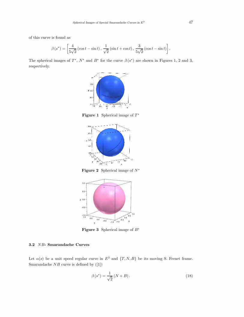
Spherical Images of Special Smarandache Curves in E3 47
of this curve is found as
β (s∗) =
[
4
5√
2(cos t − sin t) ,
1√2
(sin t + cos t) ,3
5√
2(cos t − sin t)
]
.
The spherical images of T ∗, N∗ and B∗ for the curve β (s∗) are shown in Figures 1, 2 and 3,
respectively.
Figure 1 Spherical image of T ∗
Figure 2 Spherical image of N∗
Figure 3 Spherical image of B∗
3.2 NB- Smarandache Curves
Let α(s) be a unit speed regular curve in E3 and {T, N, B} be its moving S. Frenet frame.
Smarandache NB curve is defined by ([1])
β (s∗) =1√2
(N + B) . (18)
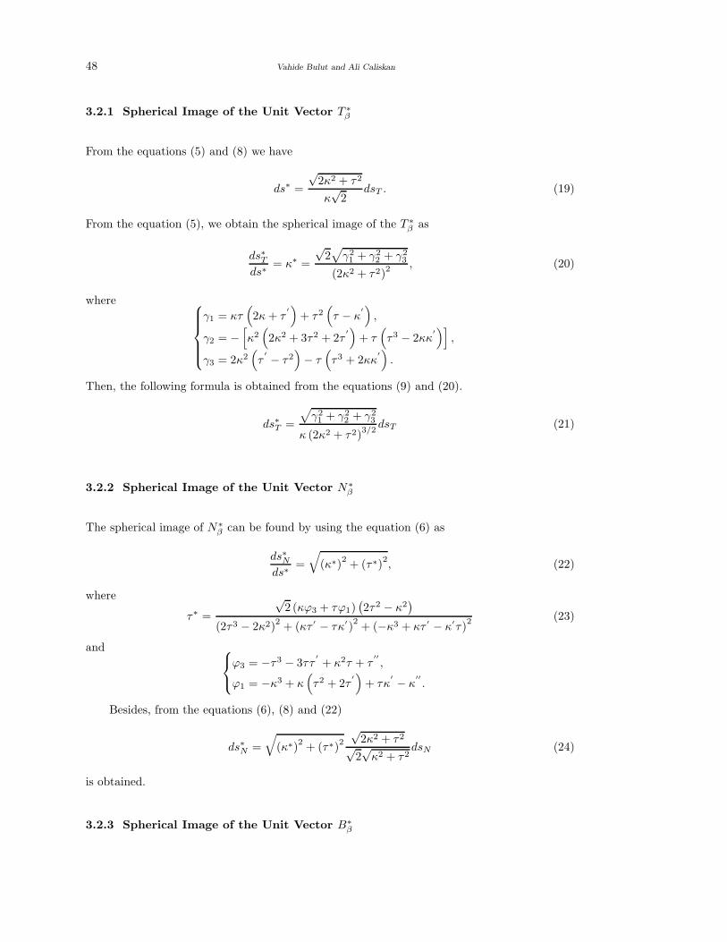
48 Vahide Bulut and Ali Caliskan
3.2.1 Spherical Image of the Unit Vector T ∗β
From the equations (5) and (8) we have
ds∗ =
√2κ2 + τ2
κ√
2dsT . (19)
From the equation (5), we obtain the spherical image of the T ∗β as
ds∗Tds∗
= κ∗ =
√2√
γ21 + γ2
2 + γ23
(2κ2 + τ2)2, (20)
where
γ1 = κτ(
2κ + τ′
)
+ τ2(
τ − κ′
)
,
γ2 = −[
κ2(
2κ2 + 3τ2 + 2τ′
)
+ τ(
τ3 − 2κκ′
)]
,
γ3 = 2κ2(
τ′ − τ2
)
− τ(
τ3 + 2κκ′
)
.
Then, the following formula is obtained from the equations (9) and (20).
ds∗T =
√
γ21 + γ2
2 + γ23
κ (2κ2 + τ2)3/2
dsT (21)
3.2.2 Spherical Image of the Unit Vector N∗β
The spherical image of N∗β can be found by using the equation (6) as
ds∗Nds∗
=
√
(κ∗)2+ (τ∗)
2, (22)
where
τ∗ =
√2 (κϕ3 + τϕ1)
(
2τ2 − κ2)
(2τ3 − 2κ2)2
+ (κτ ′ − τκ′)2
+ (−κ3 + κτ ′ − κ′τ)2 (23)
and
ϕ3 = −τ3 − 3ττ′
+ κ2τ + τ′′
,
ϕ1 = −κ3 + κ(
τ2 + 2τ′
)
+ τκ′ − κ
′′
.
Besides, from the equations (6), (8) and (22)
ds∗N =
√
(κ∗)2
+ (τ∗)2
√2κ2 + τ2
√2√
κ2 + τ2dsN (24)
is obtained.
3.2.3 Spherical Image of the Unit Vector B∗β
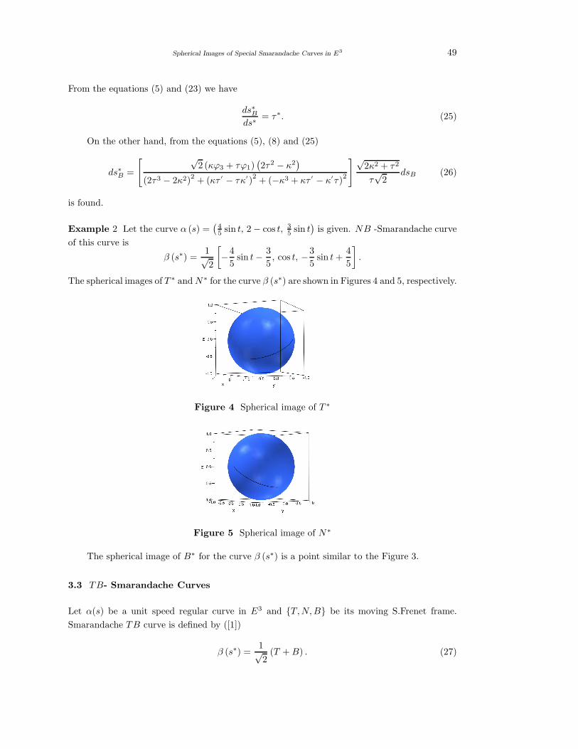
Spherical Images of Special Smarandache Curves in E3 49
From the equations (5) and (23) we have
ds∗Bds∗
= τ∗. (25)
On the other hand, from the equations (5), (8) and (25)
ds∗B =
[ √2 (κϕ3 + τϕ1)
(
2τ2 − κ2)
(2τ3 − 2κ2)2 + (κτ ′ − τκ′)2
+ (−κ3 + κτ ′ − κ′τ)2
] √2κ2 + τ2
τ√
2dsB (26)
is found.
Example 2 Let the curve α (s) =(
45 sin t, 2 − cos t, 3
5 sin t)
is given. NB -Smarandache curve
of this curve is
β (s∗) =1√2
[
−4
5sin t − 3
5, cos t, −3
5sin t +
4
5
]
.
The spherical images of T ∗ and N∗ for the curve β (s∗) are shown in Figures 4 and 5, respectively.
Figure 4 Spherical image of T ∗
Figure 5 Spherical image of N∗
The spherical image of B∗ for the curve β (s∗) is a point similar to the Figure 3.
3.3 TB- Smarandache Curves
Let α(s) be a unit speed regular curve in E3 and {T, N, B} be its moving S.Frenet frame.
Smarandache TB curve is defined by ([1])
β (s∗) =1√2
(T + B) . (27)
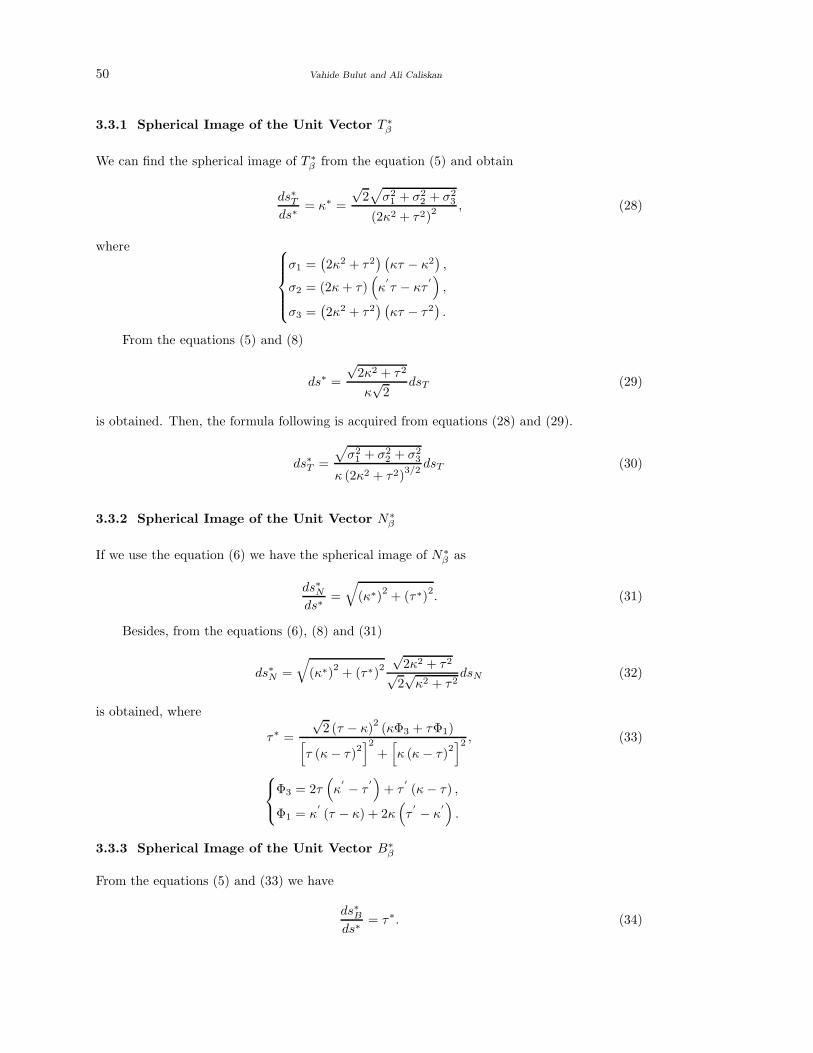
50 Vahide Bulut and Ali Caliskan
3.3.1 Spherical Image of the Unit Vector T ∗β
We can find the spherical image of T ∗β from the equation (5) and obtain
ds∗Tds∗
= κ∗ =
√2√
σ21 + σ2
2 + σ23
(2κ2 + τ2)2 , (28)
where
σ1 =(
2κ2 + τ2) (
κτ − κ2)
,
σ2 = (2κ + τ)(
κ′
τ − κτ′
)
,
σ3 =(
2κ2 + τ2) (
κτ − τ2)
.
From the equations (5) and (8)
ds∗ =
√2κ2 + τ2
κ√
2dsT (29)
is obtained. Then, the formula following is acquired from equations (28) and (29).
ds∗T =
√
σ21 + σ2
2 + σ23
κ (2κ2 + τ2)3/2
dsT (30)
3.3.2 Spherical Image of the Unit Vector N∗β
If we use the equation (6) we have the spherical image of N∗β as
ds∗Nds∗
=
√
(κ∗)2+ (τ∗)
2. (31)
Besides, from the equations (6), (8) and (31)
ds∗N =
√
(κ∗)2
+ (τ∗)2
√2κ2 + τ2
√2√
κ2 + τ2dsN (32)
is obtained, where
τ∗ =
√2 (τ − κ)
2(κΦ3 + τΦ1)
[
τ (κ − τ)2]2
+[
κ (κ − τ)2]2 , (33)
Φ3 = 2τ(
κ′ − τ
′
)
+ τ′
(κ − τ) ,
Φ1 = κ′
(τ − κ) + 2κ(
τ′ − κ
′
)
.
3.3.3 Spherical Image of the Unit Vector B∗β
From the equations (5) and (33) we have
ds∗Bds∗
= τ∗. (34)
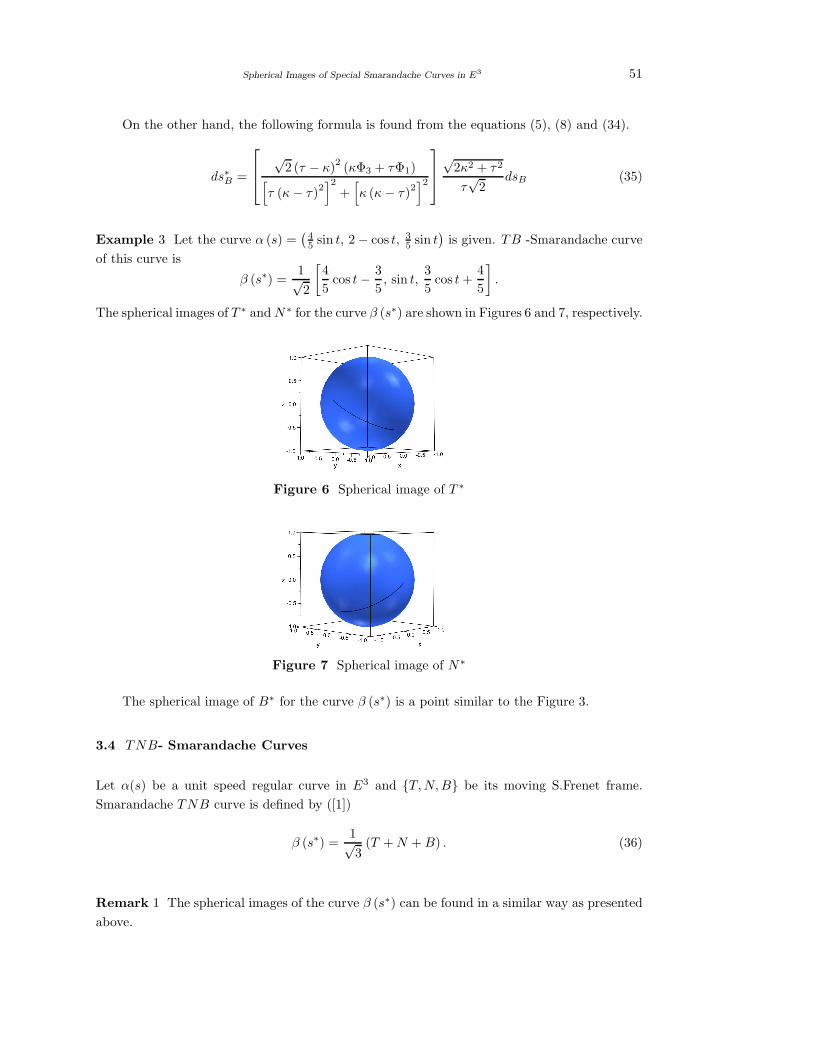
Spherical Images of Special Smarandache Curves in E3 51
On the other hand, the following formula is found from the equations (5), (8) and (34).
ds∗B =
√2 (τ − κ)
2(κΦ3 + τΦ1)
[
τ (κ − τ)2]2
+[
κ (κ − τ)2]2
√2κ2 + τ2
τ√
2dsB (35)
Example 3 Let the curve α (s) =(
45 sin t, 2 − cos t, 3
5 sin t)
is given. TB -Smarandache curve
of this curve is
β (s∗) =1√2
[
4
5cos t − 3
5, sin t,
3
5cos t +
4
5
]
.
The spherical images of T ∗ and N∗ for the curve β (s∗) are shown in Figures 6 and 7, respectively.
Figure 6 Spherical image of T ∗
Figure 7 Spherical image of N∗
The spherical image of B∗ for the curve β (s∗) is a point similar to the Figure 3.
3.4 TNB- Smarandache Curves
Let α(s) be a unit speed regular curve in E3 and {T, N, B} be its moving S.Frenet frame.
Smarandache TNB curve is defined by ([1])
β (s∗) =1√3
(T + N + B) . (36)
Remark 1 The spherical images of the curve β (s∗) can be found in a similar way as presented
above.
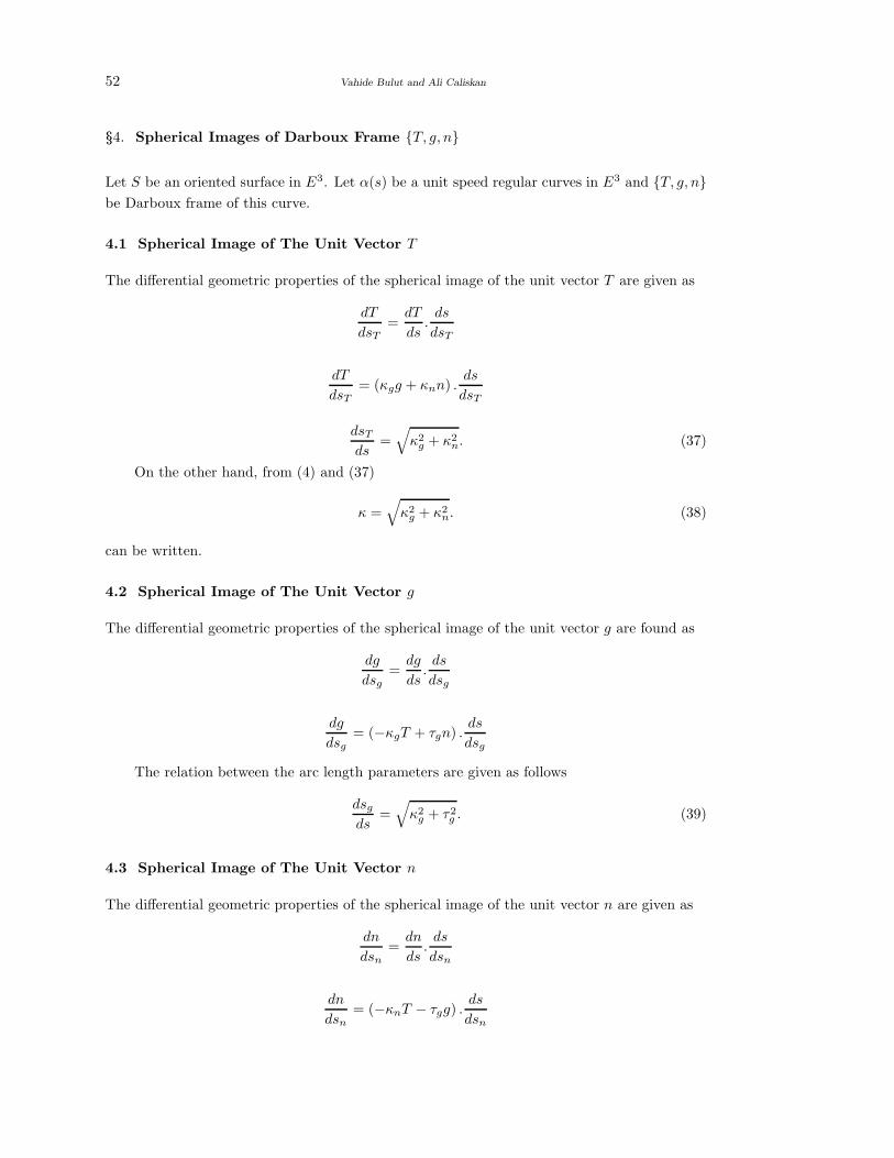
52 Vahide Bulut and Ali Caliskan
§4. Spherical Images of Darboux Frame {T, g, n}
Let S be an oriented surface in E3. Let α(s) be a unit speed regular curves in E3 and {T, g, n}be Darboux frame of this curve.
4.1 Spherical Image of The Unit Vector T
The differential geometric properties of the spherical image of the unit vector T are given as
dT
dsT=
dT
ds.
ds
dsT
dT
dsT= (κgg + κnn) .
ds
dsT
dsT
ds=√
κ2g + κ2
n. (37)
On the other hand, from (4) and (37)
κ =√
κ2g + κ2
n. (38)
can be written.
4.2 Spherical Image of The Unit Vector g
The differential geometric properties of the spherical image of the unit vector g are found as
dg
dsg=
dg
ds.ds
dsg
dg
dsg= (−κgT + τgn) .
ds
dsg
The relation between the arc length parameters are given as follows
dsg
ds=√
κ2g + τ2
g . (39)
4.3 Spherical Image of The Unit Vector n
The differential geometric properties of the spherical image of the unit vector n are given as
dn
dsn=
dn
ds.
ds
dsn
dn
dsn= (−κnT − τgg) .
ds
dsn
Spherical Images of Special Smarandache Curves in E3 53
Also, the relation between the arc length parameters is obtained as
dsn
ds=√
κ2n + τ2
g . (40)
Results:
i) If α(s) is a geodesic curve, for κg = 0,
dsT
ds= κn = κ,
dsg
ds = τg,dsn
ds=√
κ2n + τ2
g =√
κ2 + τ2g .
Also, the unit Darboux vector is as follows
c =τgT + κng√
τ2g + κ2
n
.
ii) If α(s) is an asymptotic line, for κn=0
dsT
ds= κg = κ,
dsg
ds =√
κ2g + τ2
g =√
κ2 + τ2g ,
dsn
ds= τg,
and the unit Darboux vector is
c =τgT + κgn√
τ2g + κ2
g
.
iii) If α(s) is a line of curvature, for τg=0
dsT
ds=√
κ2g + κ2
n = κ,dsg
ds = κg,dsn
ds= κn,
and the unit Darboux vector is
c =κgn + κng√
κ2g + κ2
n
.
§5. Special Smarandache Curves According To Darboux Frame In E3
5.1 Tg- Smarandache Curves
Let S be an oriented surface in E3. Let α(s) be a unit speed regular curve in E3, {T, N, B}and {T, g, n} be its S.Frenet frame and Darboux frame, respectively. Smarandache Tg curve is
defined by
β (s∗) =1√2
(T + g) . (41)
4.2 Tn- Smarandache Curves
Let S be an oriented surface in E3. Let α(s) be a unit speed regular curve in E3, {T, N, B}
54 Vahide Bulut and Ali Caliskan
and {T, g, n} be its S.Frenet frame and Darboux frame, respectively. Smarandache Tn curve is
defined by
β (s∗) =1√2
(T + n) . (42)
4.3 gn- Smarandache Curves
Let S be an oriented surface in E3. Let α(s) be a unit speed regular curve in E3, {T, N, B}and {T, g, n} be its S.Frenet frame and Darboux frame, respectively. Smarandache gn curve is
defined by
β (s∗) =1√2
(g + n) . (43)
4.4 Tgn- Smarandache Curves
Let S be an oriented surface in E3. Let α(s) be a unit speed regular curve in E3, {T, N, B}and {T, g, n} be its S.Frenet frame and Darboux frame, respectively. Smarandache Tgn curve
is defined by
β (s∗) =1√3
(T + g + n) . (44)
(See [2].)
Remark 2 The spherical images of these curves can be easily obtained by the similar way as
explained in Section 4.
§6. Conclusion
Spherical mechanisms are very important for robotics. Spherical curves which are drawn by
spherical mechanisms are used widely in kinematics and robotics. For this purpose, we presented
the spherical images of special Smarandache curves and obtained some relations between them.
References
[1] A.T.Ali, Special Smarandache curves in the Euclidean space, International Journal of
Mathematical Combinatorics, Vol.2(2010),30-36.
[2] O.Bektas and S.Yuce, Special Smarandache curves according to Darboux frame in Eu-
clidean 3- space, arXiv: 1203. 4830, 1, 2012.
[3] M.P.Do Carmo, Differential Geometry of Curves and Surfaces, Prentice Hall, Englewood
Cliffs, NJ, 1976.
[4] H.Guggenheimer, Diffrential Geometry, McGraw-Hill Book Company, 1963.
[5] E.Kreyszig, Differential Geometry, Dover Publications, 1991.
[6] B.O’Neill, Elemantery Differential Geometry, Academic press Inc. New York, 1966.
[7] M.Turgut and S.Yilmaz, Smarandache curves in Minkowski space-time, International Jour-
nal of Mathematical Combinatorics, Vol.3(2008), 51-55.
International J.Math. Combin. Vol.3(2015), 55-61
Variations of Orthogonality of Latin Squares
Vadiraja Bhatta G.R.
Department of Mathematics
Manipal Institute of Technology, Manipal University, Manipal, Karnataka-576104, India
B.R.Shankar
Department of Mathematical and Computational Sciences
National Institute of Technology, Surathkal, Karnataka, India
E-mail: [email protected]
Abstract: Orthogonal properties of Latin squares represented by permutation polynomials
are discussed. Pairs of bivariate polynomials over small rings are considered.
Key Words: Bivariate polynomials, Latin squares, orthogonal Latin squares
AMS(2010): 08B15.
§1. Introduction
1.1 Latin Squares
Combinatorial theory is one of the fastest growing areas of modern mathematics. Combinatorial
designs have wide applications in various fields, including coding theory and cryptography.
Many examples of combinatorial designs can be listed like linked design, balanced design, one-
factorization, graph etc. Latin square is one such combinatorial concept.
Definition 1.1 A Latin square of order ( or size) n is an n×n array based on some set S of n
symbols (treatments), with the property that every row and every column contains every symbol
exactly once.
In other words, every row and every column is a permutation of S. Also it can be thought
of as a two dimensional analogue of a permutation. A Latin square can be viewed as a quadruple
(R, C, S; L), where R, C, and S are sets of cardinality n, L is a mapping L : R × C → S such
that for any i ∈ R and x ∈ S, the equation
L(i, j) = x
has a unique solution j ∈ C, and for any j ∈ C, x ∈ S, the same equation has a unique solution
1Received December 21, 2014, Accepted August 12, 2015.
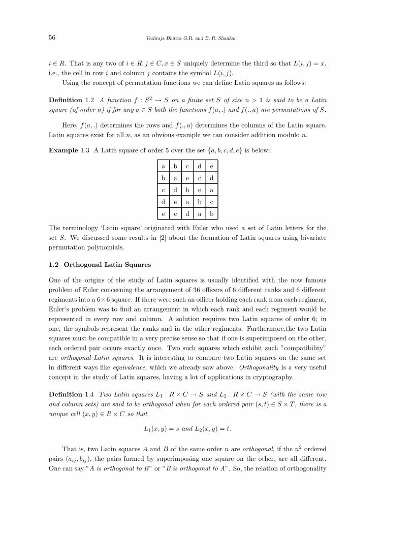
56 Vadiraja Bhatta G.R. and B. R. Shankar
i ∈ R. That is any two of i ∈ R, j ∈ C, x ∈ S uniquely determine the third so that L(i, j) = x.
i.e., the cell in row i and column j contains the symbol L(i, j).
Using the concept of permutation functions we can define Latin squares as follows:
Definition 1.2 A function f : S2 → S on a finite set S of size n > 1 is said to be a Latin
square (of order n) if for any a ∈ S both the functions f(a, .) and f(., a) are permutations of S.
Here, f(a, .) determines the rows and f(., a) determines the columns of the Latin square.
Latin squares exist for all n, as an obvious example we can consider addition modulo n.
Example 1.3 A Latin square of order 5 over the set {a, b, c, d, e} is below:
a b c d e
b a e c d
c d b e a
d e a b c
e c d a b
The terminology ‘Latin square’ originated with Euler who used a set of Latin letters for the
set S. We discussed some results in [2] about the formation of Latin squares using bivariate
permutation polynomials.
1.2 Orthogonal Latin Squares
One of the origins of the study of Latin squares is usually identified with the now famous
problem of Euler concerning the arrangement of 36 officers of 6 different ranks and 6 different
regiments into a 6×6 square. If there were such an officer holding each rank from each regiment,
Euler’s problem was to find an arrangement in which each rank and each regiment would be
represented in every row and column. A solution requires two Latin squares of order 6; in
one, the symbols represent the ranks and in the other regiments. Furthermore,the two Latin
squares must be compatible in a very precise sense so that if one is superimposed on the other,
each ordered pair occurs exactly once. Two such squares which exhibit such ”compatibility”
are orthogonal Latin squares. It is interesting to compare two Latin squares on the same set
in different ways like equivalence, which we already saw above. Orthogonality is a very useful
concept in the study of Latin squares, having a lot of applications in cryptography.
Definition 1.4 Two Latin squares L1 : R × C → S and L2 : R × C → S (with the same row
and column sets) are said to be orthogonal when for each ordered pair (s, t) ∈ S × T , there is a
unique cell (x, y) ∈ R × C so that
L1(x, y) = s and L2(x, y) = t.
That is, two Latin squares A and B of the same order n are orthogonal, if the n2 ordered
pairs (aij , bij), the pairs formed by superimposing one square on the other, are all different.
One can say ”A is orthogonal to B” or ”B is orthogonal to A”. So, the relation of orthogonality
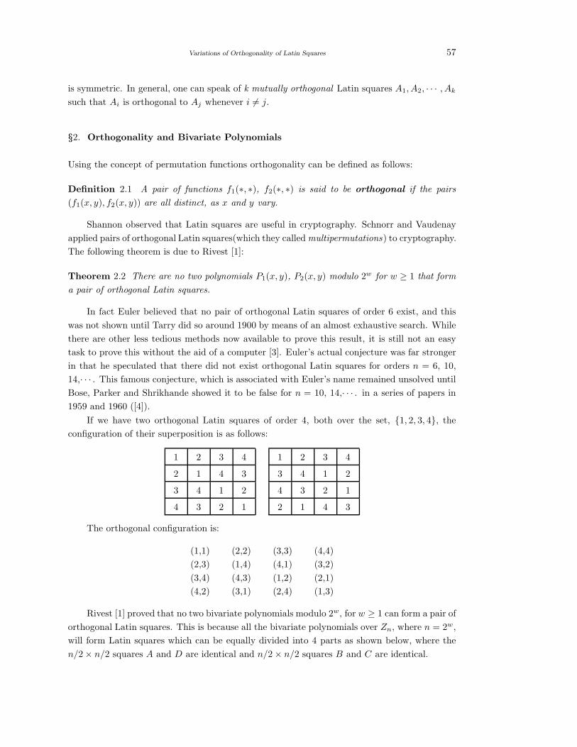
Variations of Orthogonality of Latin Squares 57
is symmetric. In general, one can speak of k mutually orthogonal Latin squares A1, A2, · · · , Ak
such that Ai is orthogonal to Aj whenever i 6= j.
§2. Orthogonality and Bivariate Polynomials
Using the concept of permutation functions orthogonality can be defined as follows:
Definition 2.1 A pair of functions f1(∗, ∗), f2(∗, ∗) is said to be orthogonal if the pairs
(f1(x, y), f2(x, y)) are all distinct, as x and y vary.
Shannon observed that Latin squares are useful in cryptography. Schnorr and Vaudenay
applied pairs of orthogonal Latin squares(which they called multipermutations) to cryptography.
The following theorem is due to Rivest [1]:
Theorem 2.2 There are no two polynomials P1(x, y), P2(x, y) modulo 2w for w ≥ 1 that form
a pair of orthogonal Latin squares.
In fact Euler believed that no pair of orthogonal Latin squares of order 6 exist, and this
was not shown until Tarry did so around 1900 by means of an almost exhaustive search. While
there are other less tedious methods now available to prove this result, it is still not an easy
task to prove this without the aid of a computer [3]. Euler’s actual conjecture was far stronger
in that he speculated that there did not exist orthogonal Latin squares for orders n = 6, 10,
14,· · · . This famous conjecture, which is associated with Euler’s name remained unsolved until
Bose, Parker and Shrikhande showed it to be false for n = 10, 14,· · · . in a series of papers in
1959 and 1960 ([4]).
If we have two orthogonal Latin squares of order 4, both over the set, {1, 2, 3, 4}, the
configuration of their superposition is as follows:
1 2 3 4
2 1 4 3
3 4 1 2
4 3 2 1
1 2 3 4
3 4 1 2
4 3 2 1
2 1 4 3
The orthogonal configuration is:
(1,1) (2,2) (3,3) (4,4)
(2,3) (1,4) (4,1) (3,2)
(3,4) (4,3) (1,2) (2,1)
(4,2) (3,1) (2,4) (1,3)
Rivest [1] proved that no two bivariate polynomials modulo 2w, for w ≥ 1 can form a pair of
orthogonal Latin squares. This is because all the bivariate polynomials over Zn, where n = 2w,
will form Latin squares which can be equally divided into 4 parts as shown below, where the
n/2 × n/2 squares A and D are identical and n/2 × n/2 squares B and C are identical.
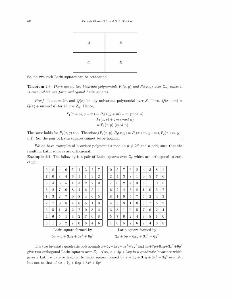
58 Vadiraja Bhatta G.R. and B. R. Shankar
A B
C D
So, no two such Latin squares can be orthogonal.
Theorem 2.3 There are no two bivariate polynomials P1(x, y) and P2(x, y) over Zn, where n
is even, which can form orthogonal Latin squares.
Proof Let n = 2m and Q(x) be any univariate polynomial over Zn.Then, Q(x + m) =
Q(x) + m(mod n) for all x ∈ Zn. Hence,
P1(x + m, y + m) = P1(x, y + m) + m (mod n)
= P1(x, y) + 2m (mod n)
= P1(x, y) (mod n)
The same holds for P2(x, y) too. Therefore,(P1(x, y), P2(x, y) = P1(x+m, y+m), P2(x+m, y+
m)). So, the pair of Latin squares cannot be orthogonal. 2We do have examples of bivariate polynomials modulo n 6= 2w and n odd, such that the
resulting Latin squares are orthogonal.
Example 2.4 The following is a pair of Latin squares over Z9 which are orthogonal to each
other.
0 8 4 6 5 1 3 2 7
7 0 8 4 6 5 1 3 2
8 4 6 5 1 3 2 7 0
3 2 7 0 8 4 6 5 1
1 3 2 7 0 8 4 6 5
2 7 0 8 4 6 5 1 3
6 5 1 3 2 7 0 8 4
4 6 5 1 3 2 7 0 8
5 1 3 2 7 0 8 4 6
Latin square formed by
5x + y + 3xy + 3x2 + 6y2
0 5 7 6 2 4 3 8 1
2 4 3 8 1 0 5 7 6
7 6 2 4 3 8 1 0 5
6 2 4 3 8 1 0 5 7
8 1 0 5 7 6 2 4 3
4 3 8 1 0 5 7 6 2
3 8 1 0 5 7 6 2 4
5 7 6 2 4 3 8 1 0
1 0 5 7 6 2 4 3 8
Latin square formed by
2x + 5y + 6xy + 3x2 + 6y2
The two bivariate quadratic polynomials x+5y+3xy+6x2+3y2 and 4x+7y+6xy+3x2+6y2
give two orthogonal Latin squares over Z9. Also, x + 4y + 3xy is a quadratic bivariate which
gives a Latin square orthogonal to Latin square formed by x + 5y + 3xy + 6x2 + 3y2 over Z9,
but not to that of 4x + 7y + 6xy + 3x2 + 6y2.
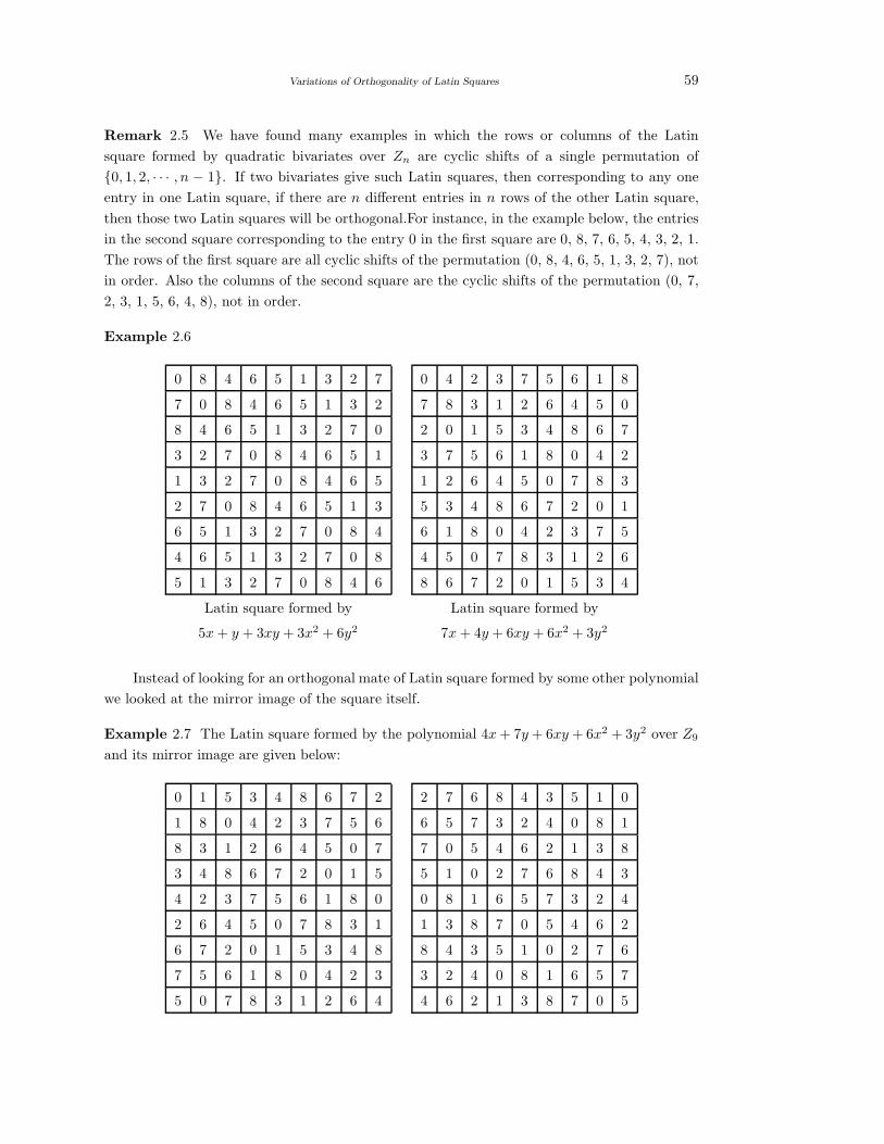
Variations of Orthogonality of Latin Squares 59
Remark 2.5 We have found many examples in which the rows or columns of the Latin
square formed by quadratic bivariates over Zn are cyclic shifts of a single permutation of
{0, 1, 2, · · · , n − 1}. If two bivariates give such Latin squares, then corresponding to any one
entry in one Latin square, if there are n different entries in n rows of the other Latin square,
then those two Latin squares will be orthogonal.For instance, in the example below, the entries
in the second square corresponding to the entry 0 in the first square are 0, 8, 7, 6, 5, 4, 3, 2, 1.
The rows of the first square are all cyclic shifts of the permutation (0, 8, 4, 6, 5, 1, 3, 2, 7), not
in order. Also the columns of the second square are the cyclic shifts of the permutation (0, 7,
2, 3, 1, 5, 6, 4, 8), not in order.
Example 2.6
0 8 4 6 5 1 3 2 7
7 0 8 4 6 5 1 3 2
8 4 6 5 1 3 2 7 0
3 2 7 0 8 4 6 5 1
1 3 2 7 0 8 4 6 5
2 7 0 8 4 6 5 1 3
6 5 1 3 2 7 0 8 4
4 6 5 1 3 2 7 0 8
5 1 3 2 7 0 8 4 6
Latin square formed by
5x + y + 3xy + 3x2 + 6y2
0 4 2 3 7 5 6 1 8
7 8 3 1 2 6 4 5 0
2 0 1 5 3 4 8 6 7
3 7 5 6 1 8 0 4 2
1 2 6 4 5 0 7 8 3
5 3 4 8 6 7 2 0 1
6 1 8 0 4 2 3 7 5
4 5 0 7 8 3 1 2 6
8 6 7 2 0 1 5 3 4
Latin square formed by
7x + 4y + 6xy + 6x2 + 3y2
Instead of looking for an orthogonal mate of Latin square formed by some other polynomial
we looked at the mirror image of the square itself.
Example 2.7 The Latin square formed by the polynomial 4x + 7y + 6xy + 6x2 + 3y2 over Z9
and its mirror image are given below:
0 1 5 3 4 8 6 7 2
1 8 0 4 2 3 7 5 6
8 3 1 2 6 4 5 0 7
3 4 8 6 7 2 0 1 5
4 2 3 7 5 6 1 8 0
2 6 4 5 0 7 8 3 1
6 7 2 0 1 5 3 4 8
7 5 6 1 8 0 4 2 3
5 0 7 8 3 1 2 6 4
2 7 6 8 4 3 5 1 0
6 5 7 3 2 4 0 8 1
7 0 5 4 6 2 1 3 8
5 1 0 2 7 6 8 4 3
0 8 1 6 5 7 3 2 4
1 3 8 7 0 5 4 6 2
8 4 3 5 1 0 2 7 6
3 2 4 0 8 1 6 5 7
4 6 2 1 3 8 7 0 5
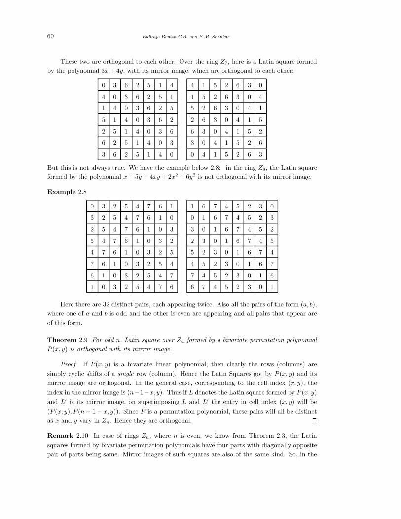
60 Vadiraja Bhatta G.R. and B. R. Shankar
These two are orthogonal to each other. Over the ring Z7, here is a Latin square formed
by the polynomial 3x + 4y, with its mirror image, which are orthogonal to each other:
0 3 6 2 5 1 4
4 0 3 6 2 5 1
1 4 0 3 6 2 5
5 1 4 0 3 6 2
2 5 1 4 0 3 6
6 2 5 1 4 0 3
3 6 2 5 1 4 0
4 1 5 2 6 3 0
1 5 2 6 3 0 4
5 2 6 3 0 4 1
2 6 3 0 4 1 5
6 3 0 4 1 5 2
3 0 4 1 5 2 6
0 4 1 5 2 6 3
But this is not always true. We have the example below 2.8: in the ring Z8, the Latin square
formed by the polynomial x + 5y + 4xy + 2x2 + 6y2 is not orthogonal with its mirror image.
Example 2.8
0 3 2 5 4 7 6 1
3 2 5 4 7 6 1 0
2 5 4 7 6 1 0 3
5 4 7 6 1 0 3 2
4 7 6 1 0 3 2 5
7 6 1 0 3 2 5 4
6 1 0 3 2 5 4 7
1 0 3 2 5 4 7 6
1 6 7 4 5 2 3 0
0 1 6 7 4 5 2 3
3 0 1 6 7 4 5 2
2 3 0 1 6 7 4 5
5 2 3 0 1 6 7 4
4 5 2 3 0 1 6 7
7 4 5 2 3 0 1 6
6 7 4 5 2 3 0 1
Here there are 32 distinct pairs, each appearing twice. Also all the pairs of the form (a, b),
where one of a and b is odd and the other is even are appearing and all pairs that appear are
of this form.
Theorem 2.9 For odd n, Latin square over Zn formed by a bivariate permutation polynomial
P (x, y) is orthogonal with its mirror image.
Proof If P (x, y) is a bivariate linear polynomial, then clearly the rows (columns) are
simply cyclic shifts of a single row (column). Hence the Latin Squares got by P (x, y) and its
mirror image are orthogonal. In the general case, corresponding to the cell index (x, y), the
index in the mirror image is (n−1−x, y). Thus if L denotes the Latin square formed by P (x, y)
and L′ is its mirror image, on superimposing L and L′ the entry in cell index (x, y) will be
(P (x, y), P (n − 1 − x, y)). Since P is a permutation polynomial, these pairs will all be distinct
as x and y vary in Zn. Hence they are orthogonal. 2Remark 2.10 In case of rings Zn, where n is even, we know from Theorem 2.3, the Latin
squares formed by bivariate permutation polynomials have four parts with diagonally opposite
pair of parts being same. Mirror images of such squares are also of the same kind. So, in the
Variations of Orthogonality of Latin Squares 61
first n/2 rows we can get n/2 distinct pairs of corresponding entries. In the last n/2 rows, these
pairs will repeat in the same order. So, these two pair of squares are not orthogonal.
§3. Conclusion
Identifying a pair of bivariate polynomials modulo n which represent a pair of orthogonal Latin
squares is not obvious. But for odd n, a Latin square formed by a bivariate polynomial is
orthogonal to its mirror image. Moreover, no two bivariate polynomials over Zn, when n is
even can form orthogonal Latin squares.
References
[1] Rivest R. L., Permutation Polynomials modulo 2w, Finite Fields and Their applications, 7
(2001) 287-292.
[2] Vadiraja Bhatta and Shankar B. R., Permutation Polynomials modulo n, n 6= 2w and Latin
Squares, International Journal Of Mathematical Combinatorics, Vol. 2 (2009) 58-65.
[3] Laywine, C.F. and Mullen, G.L., Discrete Mathematics using Latin squares, John Wiley
and Sons, Inc. (1998).
[4] Lint J.V., and Wilson R. M., A Course in Combinatorics, Cambridge University Press,
Cambridge, second edition, 2001.
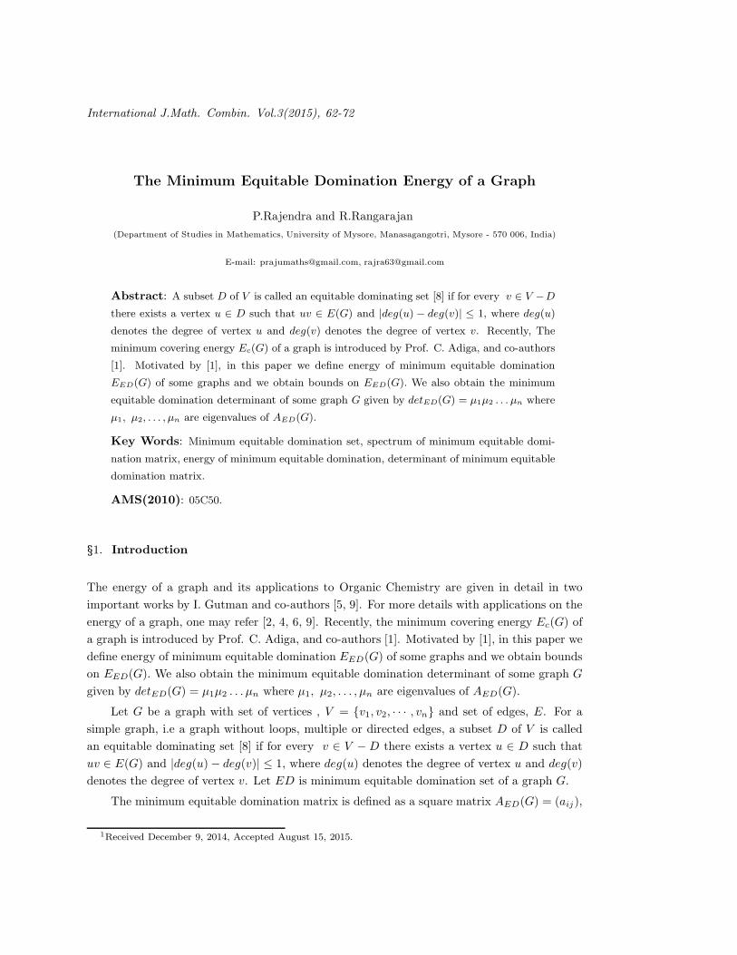
International J.Math. Combin. Vol.3(2015), 62-72
The Minimum Equitable Domination Energy of a Graph
P.Rajendra and R.Rangarajan
(Department of Studies in Mathematics, University of Mysore, Manasagangotri, Mysore - 570 006, India)
E-mail: [email protected], [email protected]
Abstract: A subset D of V is called an equitable dominating set [8] if for every v ∈ V −D
there exists a vertex u ∈ D such that uv ∈ E(G) and |deg(u) − deg(v)| ≤ 1, where deg(u)
denotes the degree of vertex u and deg(v) denotes the degree of vertex v. Recently, The
minimum covering energy Ec(G) of a graph is introduced by Prof. C. Adiga, and co-authors
[1]. Motivated by [1], in this paper we define energy of minimum equitable domination
EED(G) of some graphs and we obtain bounds on EED(G). We also obtain the minimum
equitable domination determinant of some graph G given by detED(G) = µ1µ2 . . . µn where
µ1, µ2, . . . , µn are eigenvalues of AED(G).
Key Words: Minimum equitable domination set, spectrum of minimum equitable domi-
nation matrix, energy of minimum equitable domination, determinant of minimum equitable
domination matrix.
AMS(2010): 05C50.
§1. Introduction
The energy of a graph and its applications to Organic Chemistry are given in detail in two
important works by I. Gutman and co-authors [5, 9]. For more details with applications on the
energy of a graph, one may refer [2, 4, 6, 9]. Recently, the minimum covering energy Ec(G) of
a graph is introduced by Prof. C. Adiga, and co-authors [1]. Motivated by [1], in this paper we
define energy of minimum equitable domination EED(G) of some graphs and we obtain bounds
on EED(G). We also obtain the minimum equitable domination determinant of some graph G
given by detED(G) = µ1µ2 . . . µn where µ1, µ2, . . . , µn are eigenvalues of AED(G).
Let G be a graph with set of vertices , V = {v1, v2, · · · , vn} and set of edges, E. For a
simple graph, i.e a graph without loops, multiple or directed edges, a subset D of V is called
an equitable dominating set [8] if for every v ∈ V − D there exists a vertex u ∈ D such that
uv ∈ E(G) and |deg(u) − deg(v)| ≤ 1, where deg(u) denotes the degree of vertex u and deg(v)
denotes the degree of vertex v. Let ED is minimum equitable domination set of a graph G.
The minimum equitable domination matrix is defined as a square matrix AED(G) = (aij),
1Received December 9, 2014, Accepted August 15, 2015.
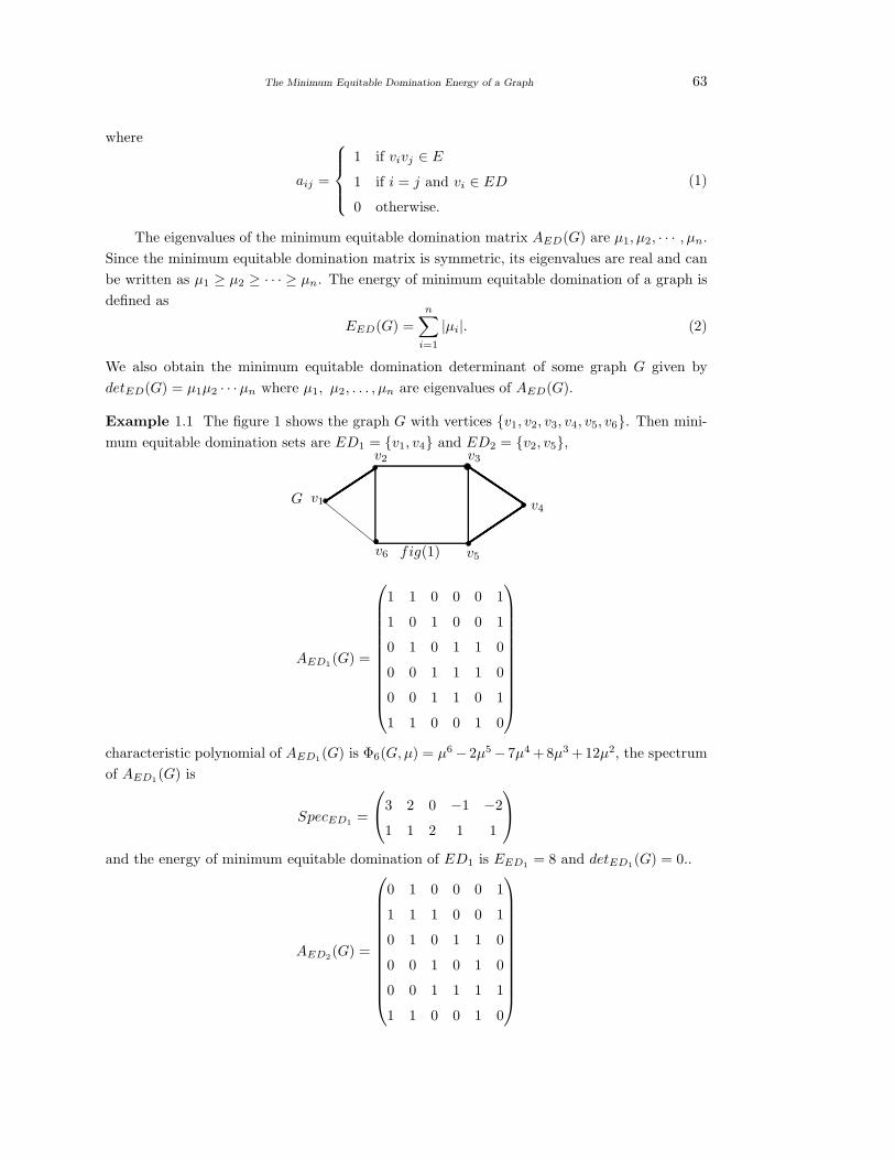
The Minimum Equitable Domination Energy of a Graph 63
where
aij =
1 if vivj ∈ E
1 if i = j and vi ∈ ED
0 otherwise.
(1)
The eigenvalues of the minimum equitable domination matrix AED(G) are µ1, µ2, · · · , µn.
Since the minimum equitable domination matrix is symmetric, its eigenvalues are real and can
be written as µ1 ≥ µ2 ≥ · · · ≥ µn. The energy of minimum equitable domination of a graph is
defined as
EED(G) =n∑
i=1
|µi|. (2)
We also obtain the minimum equitable domination determinant of some graph G given by
detED(G) = µ1µ2 · · ·µn where µ1, µ2, . . . , µn are eigenvalues of AED(G).
Example 1.1 The figure 1 shows the graph G with vertices {v1, v2, v3, v4, v5, v6}. Then mini-
mum equitable domination sets are ED1 = {v1, v4} and ED2 = {v2, v5},v2 v3
v5v6
v4v1G
fig(1)
AED1(G) =
1 1 0 0 0 1
1 0 1 0 0 1
0 1 0 1 1 0
0 0 1 1 1 0
0 0 1 1 0 1
1 1 0 0 1 0
characteristic polynomial of AED1(G) is Φ6(G, µ) = µ6 − 2µ5 − 7µ4 +8µ3 +12µ2, the spectrum
of AED1(G) is
SpecED1 =
3 2 0 −1 −2
1 1 2 1 1
and the energy of minimum equitable domination of ED1 is EED1 = 8 and detED1(G) = 0..
AED2(G) =
0 1 0 0 0 1
1 1 1 0 0 1
0 1 0 1 1 0
0 0 1 0 1 0
0 0 1 1 1 1
1 1 0 0 1 0
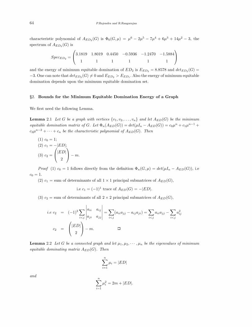
64 P.Rajendra and R.Rangarajan
characteristic polynomial of AED2(G) is Φ6(G, µ) = µ6 − 2µ5 − 7µ4 + 6µ3 + 14µ2 − 3, the
spectrum of AED2(G) is
SpecED2 =
3.1819 1.8019 0.4450 −0.5936 −1.2470 −1.5884
1 1 1 1 1 1
and the energy of minimum equitable domination of ED2 is EED2 = 8.8578 and detED2(G) =
−3. One can note that detED2(G) 6= 0 and EED2 > EED1 . Also the energy of minimum equitable
domination depends upon the minimum equitable domination set.
§2. Bounds for the Minimum Equitable Domination Energy of a Graph
We first need the following Lemma.
Lemma 2.1 Let G be a graph with vertices {v1, v2, . . . , vn} and let AED(G) be the minimum
equitable domination matrix of G. Let Φn(AED(G)) = det(µIn − AED(G)) = c0µn + c1µ
n−1 +
c2µn−2 + · · · + cn be the characteristic polynomial of AED(G). Then
(1) c0 = 1;
(2) c1 = −|ED|;
(3) c2 =
|ED|2
− m.
Proof (1) c0 = 1 follows directly from the definition Φn(G, µ) = det(µIn − AED(G)), i.e
c0 = 1.
(2) c1 = sum of determinants of all 1 × 1 principal submatrices of AED(G),
i.e c1 = (−1)1 trace of AED(G) = −|ED|.
(3) c2 = sum of determinants of all 2 × 2 principal submatrices of AED(G),
i.e c2 = (−1)2∑
i<j
∣
∣
∣
∣
∣
∣
aii aij
aji ajj
∣
∣
∣
∣
∣
∣
=∑
i<j
(aiiajj − aijaji) =∑
i<j
aiiajj −∑
i<j
a2ij
c2 =
|ED|2
− m. 2Lemma 2.2 Let G be a connected graph and let µ1, µ2, · · · , µn be the eigenvalues of minimum
equitable dominating matrix AED(G). Then
n∑
i=1
µi = |ED|
andn∑
i=1
µ2i = 2m + |ED|.
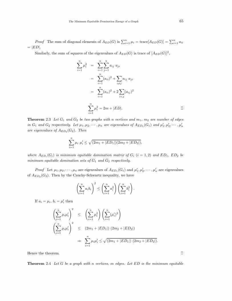
The Minimum Equitable Domination Energy of a Graph 65
Proof The sum of diagonal elements of AED(G) is∑n
i=1 µi = trace[AED(G)] =∑n
i=1 aii
= |ED|.Similarly, the sum of squares of the eigenvalues of AED(G) is trace of [AED(G)]2,
n∑
i=1
µ2i =
n∑
i=1
n∑
j=1
aij aji
=
n∑
i=1
(aii)2 +
∑
i6=j
aij aji
=n∑
i=1
(aii)2 + 2
∑
i<j
(aij)2
n∑
i=1
µ2i = 2m + |ED|. 2
Theorem 2.3 Let G1 and G2 be two graphs with n vertices and m1, m2 are number of edges
in G1 and G2 respectively. Let µ1, µ2, · · · , µn are eigenvalues of AED1(G1) and µ′1, µ
′2, · · · , µ′
n
are eigenvalues of AED2(G2). Then
n∑
i=1
µi µ′i ≤
√
(2m1 + |ED1|)(2m2 + |ED2|),
where AEDi(Gi) is minimum equitable domination matrix of Gi (i = 1, 2) and ED1, ED2 be
minimum equitable domination sets of G1 and G2 respectively.
Proof Let µ1, µ2, · · · , µn are eigenvalues of AED1(G1) and µ′1, µ
′2, · · · , µ′
n are eigenvalues
of AED2(G2). Then by the Cauchy-Schwartz inequality, we have
(
n∑
i=1
aibi
)2
≤(
n∑
i=1
a2i
)(
n∑
i=1
b2i
)
.
If ai = µi, bi = µ′i then
(
n∑
i=1
µiµ′i
)2
≤(
n∑
i=1
µ2i
)(
n∑
i=1
(µ′i)
2
)
(
n∑
i=1
µiµ′i
)2
≤ (2m1 + |ED1|) (2m2 + |ED2|)
⇒n∑
i=1
µiµ′i ≤
√
(2m1 + |ED1|) (2m2 + |ED2|).
Hence the theorem. 2Theorem 2.4 Let G be a graph with n vertices, m edges. Let ED is the minimum equitable
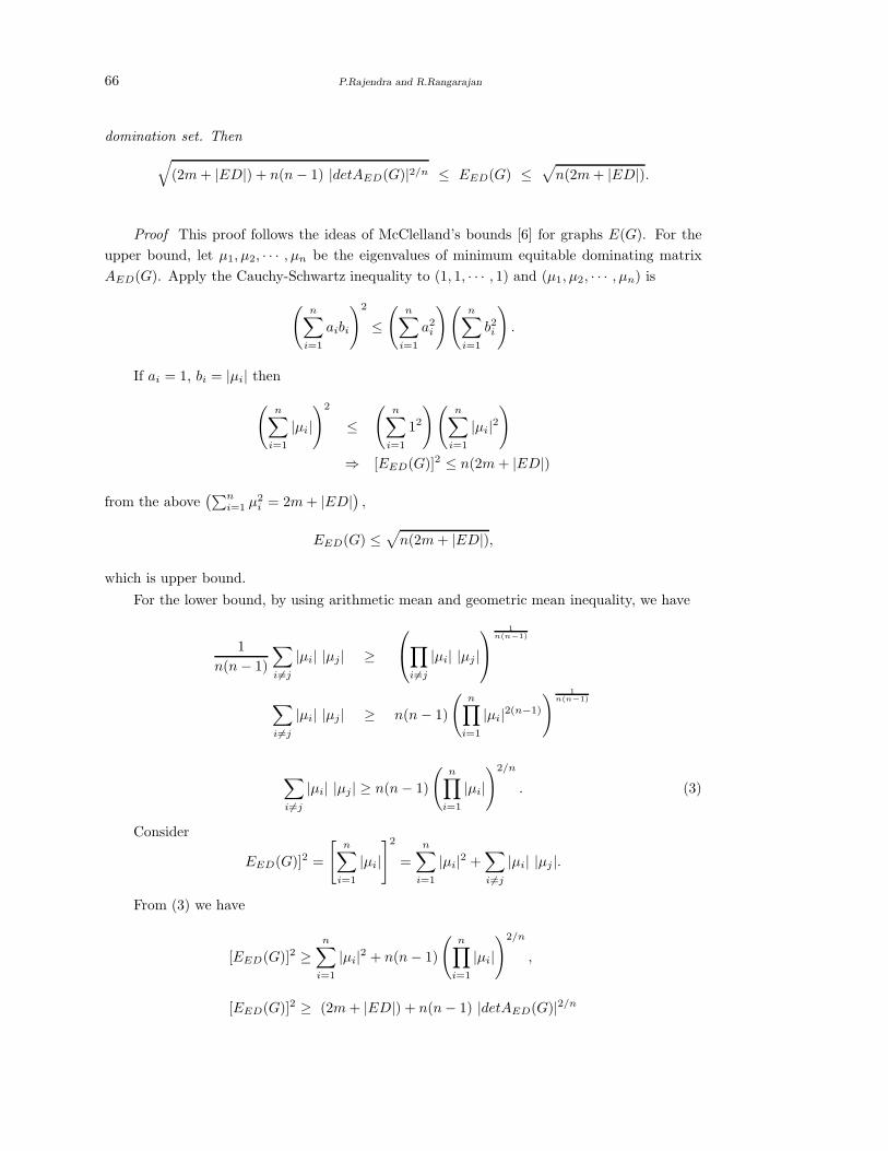
66 P.Rajendra and R.Rangarajan
domination set. Then
√
(2m + |ED|) + n(n − 1) |detAED(G)|2/n ≤ EED(G) ≤√
n(2m + |ED|).
Proof This proof follows the ideas of McClelland’s bounds [6] for graphs E(G). For the
upper bound, let µ1, µ2, · · · , µn be the eigenvalues of minimum equitable dominating matrix
AED(G). Apply the Cauchy-Schwartz inequality to (1, 1, · · · , 1) and (µ1, µ2, · · · , µn) is
(
n∑
i=1
aibi
)2
≤(
n∑
i=1
a2i
)(
n∑
i=1
b2i
)
.
If ai = 1, bi = |µi| then
(
n∑
i=1
|µi|)2
≤(
n∑
i=1
12
)(
n∑
i=1
|µi|2)
⇒ [EED(G)]2 ≤ n(2m + |ED|)
from the above(∑n
i=1 µ2i = 2m + |ED|
)
,
EED(G) ≤√
n(2m + |ED|),
which is upper bound.
For the lower bound, by using arithmetic mean and geometric mean inequality, we have
1
n(n − 1)
∑
i6=j
|µi| |µj | ≥
∏
i6=j
|µi| |µj |
1n(n−1)
∑
i6=j
|µi| |µj | ≥ n(n − 1)
(
n∏
i=1
|µi|2(n−1)
)1
n(n−1)
∑
i6=j
|µi| |µj | ≥ n(n − 1)
(
n∏
i=1
|µi|)2/n
. (3)
Consider
EED(G)]2 =
[
n∑
i=1
|µi|]2
=
n∑
i=1
|µi|2 +∑
i6=j
|µi| |µj |.
From (3) we have
[EED(G)]2 ≥n∑
i=1
|µi|2 + n(n − 1)
(
n∏
i=1
|µi|)2/n
,
[EED(G)]2 ≥ (2m + |ED|) + n(n − 1) |detAED(G)|2/n
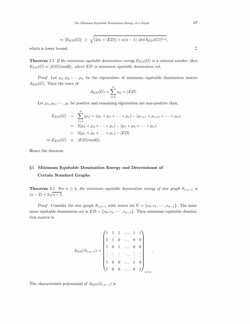
The Minimum Equitable Domination Energy of a Graph 67
⇒ [EED(G)] ≥√
(2m + |ED|) + n(n − 1) |detAED(G)|2/n,
which is lower bound. 2Theorem 2.5 If the minimum equitable domination energy EED(G) is a rational number, then
EED(G) ≡ |ED|(mod2), where ED is minimum equitable domination set.
Proof Let µ1, µ2, · · · , µn be the eigenvalues of minimum equitable domination matrix
AED(G). Then the trace of
AED(G) =
n∑
i=1
aii = |ED|.
Let µ1, µ2, · · · , µr be positive and remaining eigenvalues are non-positive then,
EED(G) =
n∑
i=1
|µi| = (µ1 + µ2 + · · · + µr) − (µr+1 + µr+2 + · · · + µn)
= 2(µ1 + µ2 + · · · + µr) − (µ1 + µ2 + · · · + µn)
= 2(µ1 + µ2 + . . . + µr) − |ED|⇒ EED(G) ≡ |ED|(mod2).
Hence the theorem. 2§3. Minimum Equitable Domination Energy and Determinant of
Certain Standard Graphs
Theorem 3.1 For n ≥ 4, the minimum equitable domination energy of star graph S1,n−1 is
(n − 2) + 2√
n − 1.
Proof Consider the star graph S1,n−1 with vertex set V = {v0, v1, · · · , vn−1}. The mini-
mum equitable domination set is ED = {v0, v1, · · · , vn−1}. Then minimum equitable domina-
tion matrix is
AED(S1,n−1) =
1 1 1 . . . 1 1
1 1 0 . . . 0 0
1 0 1 . . . 0 0...
......
. . ....
...
1 0 0 . . . 1 0
1 0 0 . . . 0 1
n×n
.
The characteristic polynomial of AED(S1,n−1) is
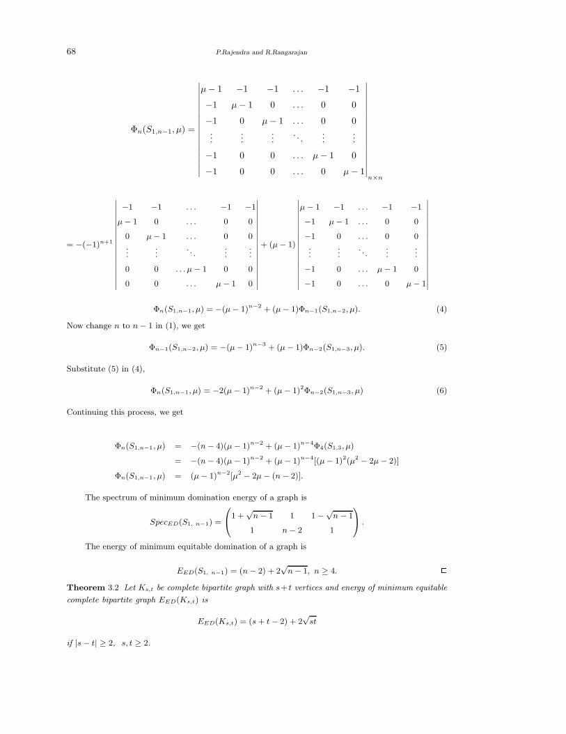
68 P.Rajendra and R.Rangarajan
Φn(S1,n−1, µ) =
∣
∣
∣
∣
∣
∣
∣
∣
∣
∣
∣
∣
∣
∣
∣
∣
∣
µ − 1 −1 −1 . . . −1 −1
−1 µ − 1 0 . . . 0 0
−1 0 µ − 1 . . . 0 0...
......
. . ....
...
−1 0 0 . . . µ − 1 0
−1 0 0 . . . 0 µ − 1
∣
∣
∣
∣
∣
∣
∣
∣
∣
∣
∣
∣
∣
∣
∣
∣
∣
n×n
= −(−1)n+1
∣
∣
∣
∣
∣
∣
∣
∣
∣
∣
∣
∣
∣
∣
∣
∣
∣
∣
−1 −1 . . . −1 −1
µ − 1 0 . . . 0 0
0 µ − 1 . . . 0 0
......
. . ....
...
0 0 . . . µ − 1 0 0
0 0 . . . µ − 1 0
∣
∣
∣
∣
∣
∣
∣
∣
∣
∣
∣
∣
∣
∣
∣
∣
∣
∣
+ (µ − 1)
∣
∣
∣
∣
∣
∣
∣
∣
∣
∣
∣
∣
∣
∣
∣
∣
∣
∣
µ − 1 −1 . . . −1 −1
−1 µ − 1 . . . 0 0
−1 0 . . . 0 0
......
. . ....
...
−1 0 . . . µ − 1 0
−1 0 . . . 0 µ − 1
∣
∣
∣
∣
∣
∣
∣
∣
∣
∣
∣
∣
∣
∣
∣
∣
∣
∣
Φn(S1,n−1, µ) = −(µ − 1)n−2 + (µ − 1)Φn−1(S1,n−2, µ). (4)
Now change n to n − 1 in (1), we get
Φn−1(S1,n−2, µ) = −(µ − 1)n−3 + (µ − 1)Φn−2(S1,n−3, µ). (5)
Substitute (5) in (4),
Φn(S1,n−1, µ) = −2(µ − 1)n−2 + (µ − 1)2Φn−2(S1,n−3, µ) (6)
Continuing this process, we get
Φn(S1,n−1, µ) = −(n − 4)(µ − 1)n−2 + (µ − 1)n−4Φ4(S1,3, µ)
= −(n − 4)(µ − 1)n−2 + (µ − 1)n−4[(µ − 1)2(µ2 − 2µ − 2)]
Φn(S1,n−1, µ) = (µ − 1)n−2[µ2 − 2µ − (n − 2)].
The spectrum of minimum domination energy of a graph is
SpecED(S1, n−1) =
1 +√
n − 1 1 1 −√
n − 1
1 n − 2 1
.
The energy of minimum equitable domination of a graph is
EED(S1, n−1) = (n − 2) + 2√
n − 1, n ≥ 4. 2Theorem 3.2 Let Ks,t be complete bipartite graph with s+ t vertices and energy of minimum equitable
complete bipartite graph EED(Ks,t) is
EED(Ks,t) = (s + t − 2) + 2√
st
if |s − t| ≥ 2, s, t ≥ 2.
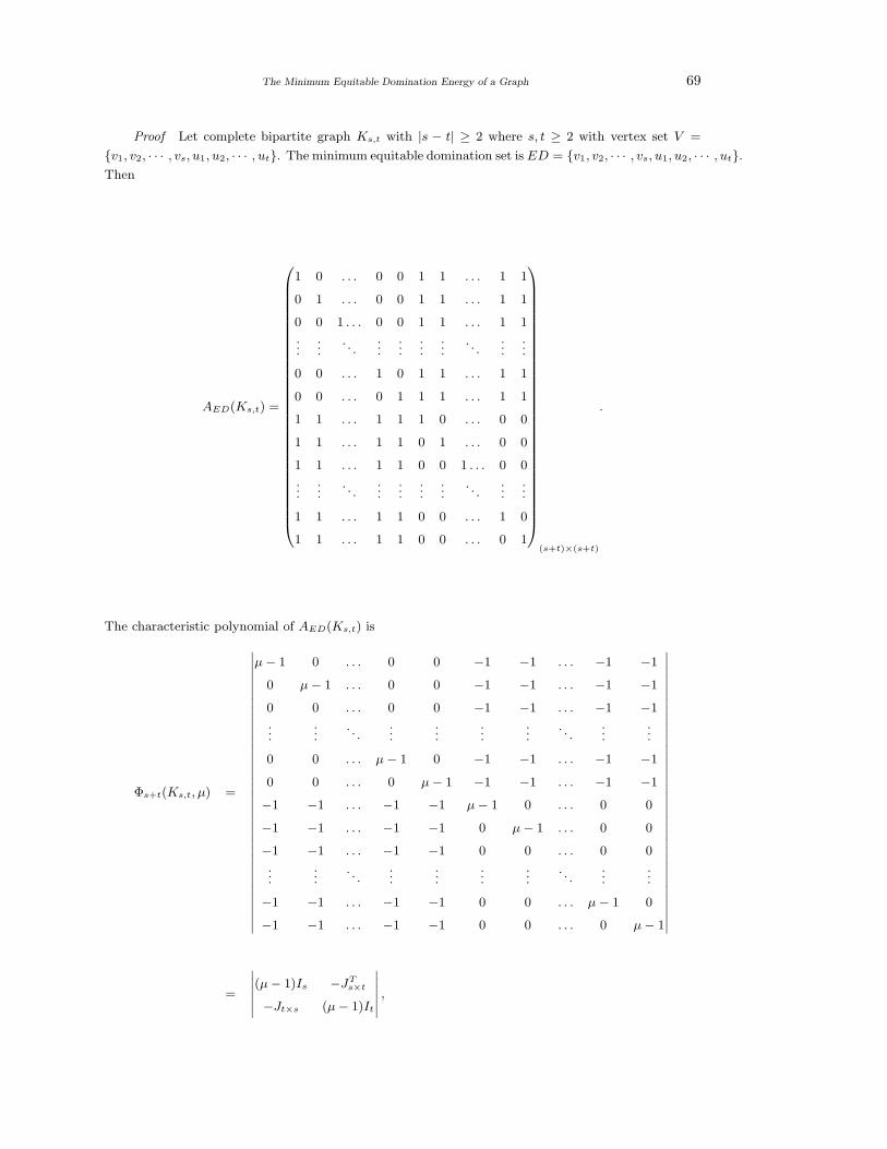
The Minimum Equitable Domination Energy of a Graph 69
Proof Let complete bipartite graph Ks,t with |s − t| ≥ 2 where s, t ≥ 2 with vertex set V =
{v1, v2, · · · , vs, u1, u2, · · · , ut}. The minimum equitable domination set is ED = {v1, v2, · · · , vs, u1, u2, · · · , ut}.Then
AED(Ks,t) =
1 0 . . . 0 0 1 1 . . . 1 1
0 1 . . . 0 0 1 1 . . . 1 1
0 0 1 . . . 0 0 1 1 . . . 1 1
......
. . ....
......
.... . .
......
0 0 . . . 1 0 1 1 . . . 1 1
0 0 . . . 0 1 1 1 . . . 1 1
1 1 . . . 1 1 1 0 . . . 0 0
1 1 . . . 1 1 0 1 . . . 0 0
1 1 . . . 1 1 0 0 1 . . . 0 0
......
. . ....
......
.... . .
......
1 1 . . . 1 1 0 0 . . . 1 0
1 1 . . . 1 1 0 0 . . . 0 1
(s+t)×(s+t)
.
The characteristic polynomial of AED(Ks,t) is
Φs+t(Ks,t, µ) =
∣
∣
∣
∣
∣
∣
∣
∣
∣
∣
∣
∣
∣
∣
∣
∣
∣
∣
∣
∣
∣
∣
∣
∣
∣
∣
∣
∣
∣
∣
∣
∣
∣
∣
∣
∣
µ − 1 0 . . . 0 0 −1 −1 . . . −1 −1
0 µ − 1 . . . 0 0 −1 −1 . . . −1 −1
0 0 . . . 0 0 −1 −1 . . . −1 −1
......
. . ....
......
.... . .
......
0 0 . . . µ − 1 0 −1 −1 . . . −1 −1
0 0 . . . 0 µ − 1 −1 −1 . . . −1 −1
−1 −1 . . . −1 −1 µ − 1 0 . . . 0 0
−1 −1 . . . −1 −1 0 µ − 1 . . . 0 0
−1 −1 . . . −1 −1 0 0 . . . 0 0
......
. . ....
......
.... . .
......
−1 −1 . . . −1 −1 0 0 . . . µ − 1 0
−1 −1 . . . −1 −1 0 0 . . . 0 µ − 1
∣
∣
∣
∣
∣
∣
∣
∣
∣
∣
∣
∣
∣
∣
∣
∣
∣
∣
∣
∣
∣
∣
∣
∣
∣
∣
∣
∣
∣
∣
∣
∣
∣
∣
∣
∣
=
∣
∣
∣
∣
∣
∣
(µ − 1)Is −JTs×t
−Jt×s (µ − 1)It
∣
∣
∣
∣
∣
∣
,
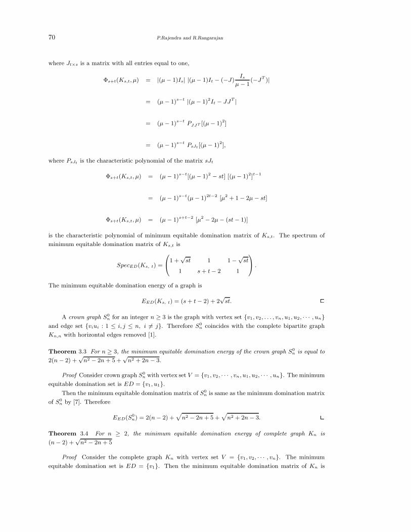
70 P.Rajendra and R.Rangarajan
where Jt×s is a matrix with all entries equal to one,
Φs+t(Ks,t, µ) = |(µ − 1)Is| |(µ − 1)It − (−J)Is
µ − 1(−JT )|
= (µ − 1)s−t |(µ − 1)2It − JJT |
= (µ − 1)s−t PJJT [(µ − 1)2]
= (µ − 1)s−t PsJt [(µ − 1)2],
where PsJt is the characteristic polynomial of the matrix sJt
Φs+t(Ks,t, µ) = (µ − 1)s−t[(µ − 1)2 − st] [(µ − 1)2]t−1
= (µ − 1)s−t(µ − 1)2t−2 [µ2 + 1 − 2µ − st]
Φs+t(Ks,t, µ) = (µ − 1)s+t−2 [µ2 − 2µ − (st − 1)]
is the characteristic polynomial of minimum equitable domination matrix of Ks,t. The spectrum of
minimum equitable domination matrix of Ks,t is
SpecED(Ks, t) =
1 +√
st 1 1 −√
st
1 s + t − 2 1
.
The minimum equitable domination energy of a graph is
EED(Ks, t) = (s + t − 2) + 2√
st. 2A crown graph S0
n for an integer n ≥ 3 is the graph with vertex set {v1, v2, . . . , vn, u1, u2, · · · , un}and edge set {viui : 1 ≤ i, j ≤ n, i 6= j}. Therefore S0
n coincides with the complete bipartite graph
Kn,n with horizontal edges removed [1].
Theorem 3.3 For n ≥ 3, the minimum equitable domination energy of the crown graph S0n is equal to
2(n − 2) +√
n2 − 2n + 5 +√
n2 + 2n − 3.
Proof Consider crown graph S0n with vertex set V = {v1, v2, · · · , vn, u1, u2, · · · , un}. The minimum
equitable domination set is ED = {v1, u1}.Then the minimum equitable domination matrix of S0
n is same as the minimum domination matrix
of S0n by [7]. Therefore
EED(S0n) = 2(n − 2) +
√
n2 − 2n + 5 +√
n2 + 2n − 3. 2Theorem 3.4 For n ≥ 2, the minimum equitable domination energy of complete graph Kn is
(n − 2) +√
n2 − 2n + 5
Proof Consider the complete graph Kn with vertex set V = {v1, v2, · · · , vn}. The minimum
equitable domination set is ED = {v1}. Then the minimum equitable domination matrix of Kn is
The Minimum Equitable Domination Energy of a Graph 71
same as the minimum domination matrix of Kn by [7]. Therefore,
EED(Kn) = (n − 2) +√
n2 − 2n + 5. 2Let us obtain the minimum equitable domination determinant of some graph G given by detED(G) =
µ1µ2 · · ·µn, where µ1, µ2, · · · , µn are eigenvalues of AED(G).
Proposition 3.5 Let S1,n−1 (n ≥ 4), Kn (n ≥ 2) be the star and complete graphs with n vertices,
respectively, S0n (n ≥ 3), is crown graph with 2n vertices and Ks,t (|s− t| ≥ 2) be the complete bipartite
graph with s + t vertices. Then
(1) detED(S1,n−1) = −(n − 2);
(2) detED(Kn) = (−1)(n−1);
(3) detED(Ks,t) = (1 − st);
(4) detED(S0n) = (−1)n−1(3 − 2n).
Proof w.k.t detED(G) = µ1 µ2 · · ·µn, where µ1, µ2, · · · , µn are eigenvalues of G.
Case 1. detED(S1,n−1) = (1 +√
n − 1)1 1n−2 (1 −√
n − 1)1 = −(n − 2), where n ≥ 4.
Case 2.
detED(Kn) =
(
(n − 1) +√
n2 − 2n + 5
2
)1
(−1)n−2
(
(n − 1) −√
n2 − 2n + 5
2
)1
= (−1)n−1, where n ≥ 2.
Case 3. detED(Ks,t) = (1 +√
st)1 (1)s+t−2 (1 −√
st)1 = (1 − st), where |s − t| ≥ 2.
Case 4.
detED(S0n) =
(
(n − 1) ±√
n2 − 2n + 5
2
)1 ((3 − n) ±
√n2 + 2n − 3
2
)1
(1)n−2(−1)n−2
= (−1)n−1(3 − 2n),
where n ≥ 3. 2Theorem 3.6 If the graph G is non-singular (i.e no eigenvalues of AED(G) is equal to zero) then
EED(G) ≥ n, (non-hypoenergetic).
Proof. Let µ1, µ2, · · · , µn are non-zero eigenvalues of AED(G). Then inequality between the
arithmetic and geometric mean, we have
dv
dx
|µ1| + |µ2| + · · · + |µn|n
≥ (|µ1||µ2| · · · |µn|)1/n
1
nEED(G) ≥ (detAED(G))1/n.
The determinant of the AED(G) matrix is necessary an integer. Because no eigenvalues is zero,
|detAED(G)| ≥ 1 then |detAED(G)|1/n ≥ 1. Therefore EED(G) ≥ n. 2Acknowledgement We acknowledge duly that the present research work is supported by the UGC-
BSR Fellowship, Government of India, grant No.F.7-349/2011 and UGC-SAP, DRS-I, No. F.510/2/DRS
/2011(SAP-I).
72 P.Rajendra and R.Rangarajan
References
[1] C.Adiga, A.Bayad, I.Gutman and Shrikanth. A. S, The minimum covering energy of a graph,
Krag. J. Sci., 34 (2012), 39-56.
[2] R.B.Bapat, Graphs and Matrices, Hindustan Book Agency (2011).
[3] R.B.Bapat, S.Pati, Energy of a graph is never an odd integer, Bull. Kerala Math. Assoc., 1
(2011), 129-132.
[4] D.M.Cvetkovic, M.Doob and H.Sachs, Spectra of Graphs, Theory and Application, Academic Press,
New York, USA, 1980.
[5] I.Gutman, The energy of a graph, Ber. Math-Statist. Sekt. Forschungsz. Graz, 103 (1978), 1-22.
[6] B.J.McClelland, Properties of the latent roots of a matrix: The estimation of π-electron energies,
J. Chem. Phys., 54 (1971), 640-643.
[7] M.R.Rajesh Kanna, B.N.Dharmendra and G.Sridhara, The minimum dominating energy of a
eraph, Int. J. of Pure and Appl. Math., 85(4), 2013, 707-718.
[1] V.Swaminathan and K.M.Dharmalingam, Degree equitable domination on graphs, Krag. J. of
Math., 35 (1) (2011), 191-197.
[9] X. Li, Y.Shi and I. utman, Graph Energy, Springer New York, 2012.
International J.Math. Combin. Vol.3(2015), 73-80
Some Results on Relaxed Mean Labeling
V.Maheswari1 , D.S.T.Ramesh2 and V.Balaji3
1. Department of Mathematics, KCG College of Engineering and Technology, Chennai-600 095, India
2. Department of Mathematics, Margoschis College, Nazareth-628617, India
3. Department of Mathematics, Sacred Heart College, Tirupattur-635 601, India
E-mail: [email protected]
Abstract: In this paper, we investigate relaxed mean labeling of some standard graphs.
We prove, any cycle is a relaxed mean graph; if n > 4, Kn is not a relaxed mean graph;
K2,n is a relaxed mean graph for all n; any Triangular snake is a relaxed mean graph; any
Quadrilateral snake is a relaxed mean graph; the graph P 2n is a relaxed mean graph; Ln Θ K1
is a relaxed mean graph. Also, we prove Kcn + 2K2 is a relaxed mean graph for all n; W4 is
a relaxed mean graph; K2 + mK1 is a relaxed mean graph for all m; if G1 and G2 are tree,
then G = G1 ∪ G2 is a relaxed mean graph; the planar grid Pm × Pn is a relaxed mean
graph for m > 2, n > 2 and the prism Pm × Cn is a relaxed mean graph for m > 2 and for
all n > 3.
Key Words: Smarandache relaxed k-mean graph, relaxed mean graph, cycle, path, star.
AMS(2010): 05C78.
§1. Introduction
All graphs in this paper are finite, simple an undirected. Terms not defined here are used in the sense
of Harary [3]. In 1966, Rosa [5] introduced β-valuation of graph. Golomb subsequently called such
a labeling graceful. In 1980, Graham and Sloane [2] introduced the harmonious labeling of a graph.
Also, in 2003, Somasundaram and Ponraj [6] and [7] introduced the mean labeling of a graph. On
similar lines, we define relaxed mean labeling. In [4], we proved any path is a relaxed mean graph and
if m = 5, K1,m is not a relaxed mean graph. We proved the bistar Bm,n is a relaxed mean graph if
|m−n| = 3. Also, we proved that combs are relaxed mean graph and C3 ∪ Pn is a relaxed mean graph
for n = 2. In this paper, we prove any cycle is a relaxed mean graph; if n > 4, Kn is not a relaxed
mean graph; K2,n is a relaxed mean graph for all n; any Triangular snake is a relaxed mean graph;
any Quadrilateral snake is a relaxed mean graph; the graph P2n is a relaxed mean graph; Ln Θ K1 is a
relaxed mean graph and Kcn +2K2 is a relaxed mean graph for all n. Also, we prove W4 is a relaxed
mean graph; K2+ mK1 is a relaxed mean graph for all m; If G1 and G2 are trees, then G = G1 ∪ G2
is a relaxed mean graph; the planar grid Pm×Pn is a relaxed mean graph for m > 2, n > 2 and the
prism Pm×Cn is a relaxed mean graph for m > 2 and for all n > 3. The condition for a graph to be
relaxed mean is that p = q + 1 in [4].
1Received December 9, 2014, Accepted August 18, 2015.
74 V.Maheswari, D.S.T.Ramesh and V.Balaji
§2. Main Results
Definition 2.1 A graph G = (V, E) with p vertices and q edges is said to be a Smarandache relaxed
k-mean graph if there exists a function f from the vertex set of G to {0, 1, 2, 3, · · · , q + 1} such that in
the induced map f∗ from the edge set of G to {1, 2, 3, · · · , q} defined by
f ∗ (e = uv) =
f(u) + f(v)
2if f(u) + f(v) is even
f(u) + f(v) + 1
2if f(u) + f(v) is odd, then
the resulting edge labels are distinct. Furthermore, such a graph is called a Smarandache relaxed k-mean
graph if we replace 2 by k and f ∗ (uv) by
⌊
f(u) + f(v)
k
⌋
.
Theorem 2.2 Any cycle is a relaxed mean graph.
Proof The proof is divided into two cases following.
Case 1. Let n be odd. Let Cn be a cycle u1u2 · · ·unu1. Define f : V(Cn) → {0, 1, 2, · · · , q = n}and q + 1 = n + 1 by f(u1) = 0 ; f(un) = n + 1; f(ui) = i − 1 for 2 6 i 6
n− 1
2and f(uj) = j for
n + 1
26 j 6 n− 1.
Case 2. Let n be even. Let Cn be a cycle u1u2 · · · nu1. Define f : V(Cn) → {0, 1, 2, · · · , q = n}and q + 1 = n + 1 by f(u1) = 0 ; f(un) = n + 1; f(ui) = i – 1 for 2 6 i 6
n
2and f(uj) = j for
n
2+ 1 6 j 6 n− 1.
Therefore, the set of labels of the edges of Cn is {1, 2, . . . , n}. Hence Cn is a relaxed mean graph.2Theorem 2.3 If n > 4, Kn is not a relaxed mean graph.
Proof Suppose n > 4, Kn is a relaxed mean graph. To get the edge label q + 1 =n(n − 1)
2+ 1,
we must have q + 1 and q − 2 as the vertex labels. Let u and v be the vertices whose vertex labels are
q + 1 and q − 2 respectively.
To get the edge label 1 we must have 0 and 1 as the vertex label (or) 0 and 2 as the vertex label.
In either case 0 must be a label of some vertex. Let w be the vertex whose vertex label is 0.
If q + 1 is even, the edges uw and vw get the same labelq + 2
2which should not happen. If q + 1
is odd and 0,1 are the vertex labels with labels w1 having vertex label 1, then the edges uw and uw1
get the same labelq + 2
2; if q is odd and 0, 2 are the vertex labels with w1 having vertex label 2, then
the edges uw and vw1 get the same labelq + 2
2which again should not happen. Hence Kn is not a
relaxed mean graph for n > 4. 2Theorem 2.4 K2,n is a relaxed mean graph for all n.
Proof Let (V1, V2) be the bipartition of K2,n with V1= {u, v}, V2 = {u1, u2, · · · , un}. Define
f: V(K2,n) → {0, 1, 2, . . . , q = 2n} and q + 1 = 2n + 1 by f(u) = 1; f(v) = 2n + 1; f(u1) = 0 and
f(ui+1) = 2i for 1 6 i 6 n − 1.
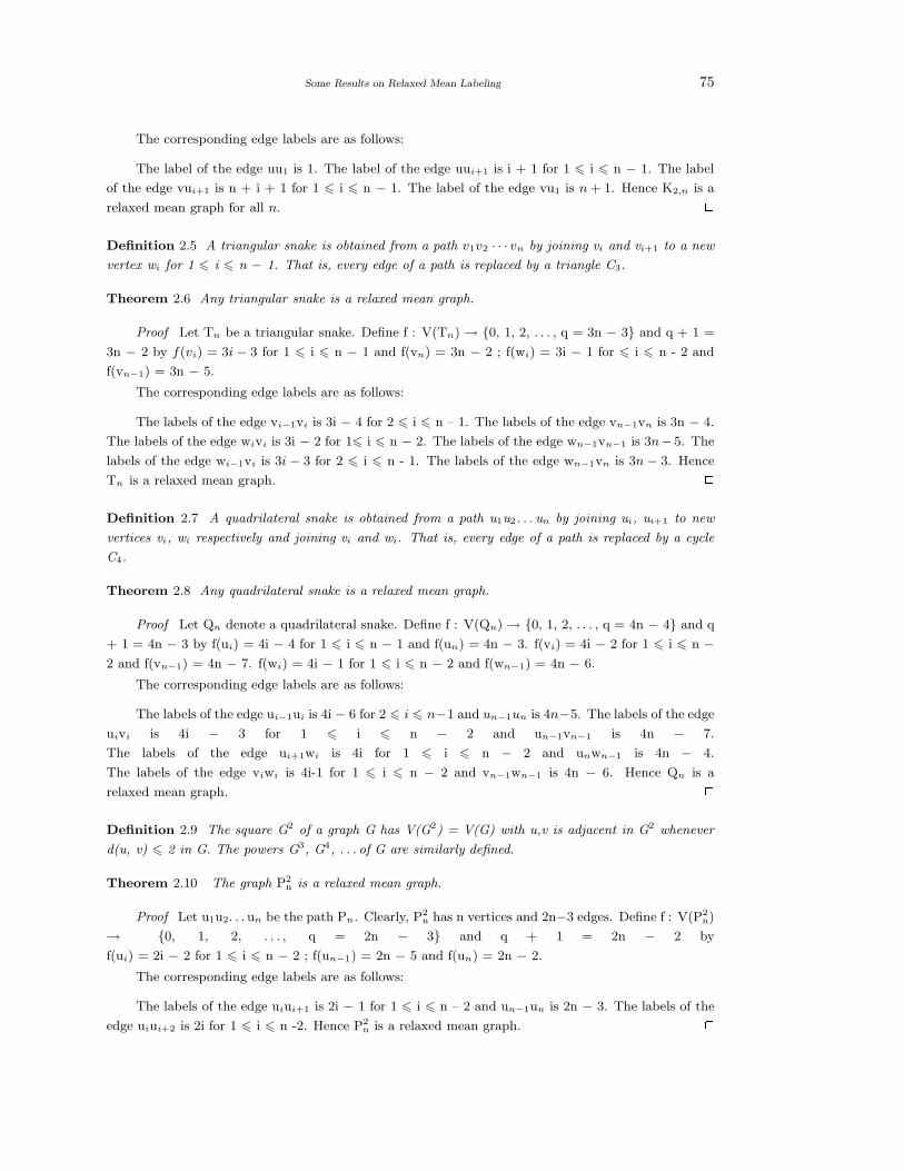
Some Results on Relaxed Mean Labeling 75
The corresponding edge labels are as follows:
The label of the edge uu1 is 1. The label of the edge uui+1 is i + 1 for 1 6 i 6 n − 1. The label
of the edge vui+1 is n + i + 1 for 1 6 i 6 n − 1. The label of the edge vu1 is n + 1. Hence K2,n is a
relaxed mean graph for all n. 2Definition 2.5 A triangular snake is obtained from a path v1v2 · · · vn by joining vi and vi+1 to a new
vertex wi for 1 6 i 6 n − 1. That is, every edge of a path is replaced by a triangle C3.
Theorem 2.6 Any triangular snake is a relaxed mean graph.
Proof Let Tn be a triangular snake. Define f : V(Tn) → {0, 1, 2, . . . , q = 3n − 3} and q + 1 =
3n − 2 by f(vi) = 3i − 3 for 1 6 i 6 n − 1 and f(vn) = 3n − 2 ; f(wi) = 3i − 1 for 6 i 6 n - 2 and
f(vn−1) = 3n − 5.
The corresponding edge labels are as follows:
The labels of the edge vi−1vi is 3i − 4 for 2 6 i 6 n – 1. The labels of the edge vn−1vn is 3n − 4.
The labels of the edge wivi is 3i − 2 for 16 i 6 n − 2. The labels of the edge wn−1vn−1 is 3n− 5. The
labels of the edge wi−1vi is 3i − 3 for 2 6 i 6 n - 1. The labels of the edge wn−1vn is 3n − 3. Hence
Tn is a relaxed mean graph. 2Definition 2.7 A quadrilateral snake is obtained from a path u1u2. . . un by joining ui, ui+1 to new
vertices vi, wi respectively and joining vi and wi. That is, every edge of a path is replaced by a cycle
C4.
Theorem 2.8 Any quadrilateral snake is a relaxed mean graph.
Proof Let Qn denote a quadrilateral snake. Define f : V(Qn) → {0, 1, 2, . . . , q = 4n − 4} and q
+ 1 = 4n − 3 by f(ui) = 4i − 4 for 1 6 i 6 n − 1 and f(un) = 4n − 3. f(vi) = 4i − 2 for 1 6 i 6 n −2 and f(vn−1) = 4n − 7. f(wi) = 4i − 1 for 1 6 i 6 n − 2 and f(wn−1) = 4n − 6.
The corresponding edge labels are as follows:
The labels of the edge ui−1ui is 4i − 6 for 2 6 i 6 n−1 and un−1un is 4n−5. The labels of the edge
uivi is 4i − 3 for 1 6 i 6 n − 2 and un−1vn−1 is 4n − 7.
The labels of the edge ui+1wi is 4i for 1 6 i 6 n − 2 and unwn−1 is 4n − 4.
The labels of the edge viwi is 4i-1 for 1 6 i 6 n − 2 and vn−1wn−1 is 4n − 6. Hence Qn is a
relaxed mean graph. 2Definition 2.9 The square G2 of a graph G has V(G2) = V(G) with u,v is adjacent in G2 whenever
d(u, v) 6 2 in G. The powers G3, G4, . . . of G are similarly defined.
Theorem 2.10 The graph P2n is a relaxed mean graph.
Proof Let u1u2. . . un be the path Pn. Clearly, P2n has n vertices and 2n−3 edges. Define f : V(P2
n)
→ {0, 1, 2, . . . , q = 2n − 3} and q + 1 = 2n − 2 by
f(ui) = 2i − 2 for 1 6 i 6 n − 2 ; f(un−1) = 2n − 5 and f(un) = 2n − 2.
The corresponding edge labels are as follows:
The labels of the edge uiui+1 is 2i − 1 for 1 6 i 6 n – 2 and un−1un is 2n − 3. The labels of the
edge uiui+2 is 2i for 1 6 i 6 n -2. Hence P2n is a relaxed mean graph. 2
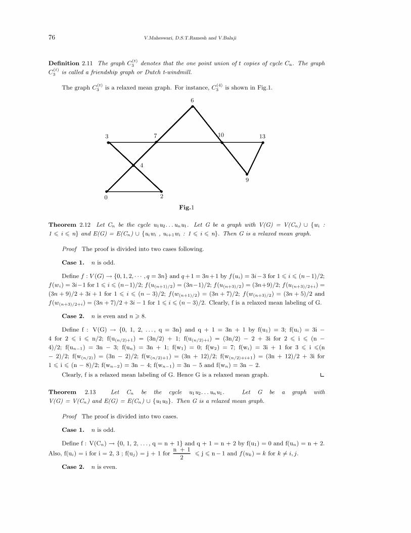
76 V.Maheswari, D.S.T.Ramesh and V.Balaji
Definition 2.11 The graph C(t)3 denotes that the one point union of t copies of cycle Cn. The graph
C(t)3 is called a friendship graph or Dutch t-windmill.
The graph C(t)3 is a relaxed mean graph. For instance, C
(4)3 is shown in Fig.1.
6
3 7 10 13
9
4
0 2
Fig.1
Theorem 2.12 Let Cn be the cycle u1u2. . . unu1. Let G be a graph with V(G) = V(Cn) ∪ {wi :
1 6 i 6 n} and E(G) = E(Cn) ∪ {uiwi , ui+1wi : 1 6 i 6 n}. Then G is a relaxed mean graph.
Proof The proof is divided into two cases following.
Case 1. n is odd.
Define f : V (G) → {0, 1, 2, · · · , q = 3n} and q +1 = 3n+1 by f(ui) = 3i−3 for 1 6 i 6 (n−1)/2;
f(wi) = 3i−1 for 1 6 i 6 (n−1)/2; f(u(n+1)/2) = (3n−1)/2; f(u(n+3)/2) = (3n+9)/2; f(u(n+3)/2+i) =
(3n + 9)/2 + 3i + 1 for 1 6 i 6 (n − 3)/2; f(w(n+1)/2) = (3n + 7)/2; f(w(n+3)/2) = (3n + 5)/2 and
f(w(n+3)/2+i) = (3n + 7)/2 + 3i − 1 for 1 6 i 6 (n − 3)/2. Clearly, f is a relaxed mean labeling of G.
Case 2. n is even and n > 8.
Define f : V(G) → {0, 1, 2, . . . , q = 3n} and q + 1 = 3n + 1 by f(u1) = 3; f(ui) = 3i −4 for 2 6 i 6 n/2; f(u(n/2)+1) = (3n/2) + 1; f(u(n/2)+i) = (3n/2) − 2 + 3i for 2 6 i 6 (n −4)/2; f(un−1) = 3n − 3; f(un) = 3n + 1; f(w1) = 0; f(w2) = 7; f(wi) = 3i + 1 for 3 6 i 6(n
− 2)/2; f(w(n/2)) = (3n − 2)/2; f(w(n/2)+1) = (3n + 12)/2; f(w(n/2)+i+1) = (3n + 12)/2 + 3i for
1 6 i 6 (n − 8)/2; f(wn−2) = 3n − 4; f(wn−1) = 3n − 5 and f(wn) = 3n − 2.
Clearly, f is a relaxed mean labeling of G. Hence G is a relaxed mean graph. 2Theorem 2.13 Let Cn be the cycle u1u2. . . unu1. Let G be a graph with
V(G) = V(Cn) and E(G) = E(Cn) ∪ {u1u3}. Then G is a relaxed mean graph.
Proof The proof is divided into two cases.
Case 1. n is odd.
Define f : V(Cn) → {0, 1, 2, . . . , q = n + 1} and q + 1 = n + 2 by f(u1) = 0 and f(un) = n + 2.
Also, f(ui) = i for i = 2, 3 ; f(uj) = j + 1 forn + 1
26 j 6 n− 1 and f(uk) = k for k 6= i, j.
Case 2. n is even.
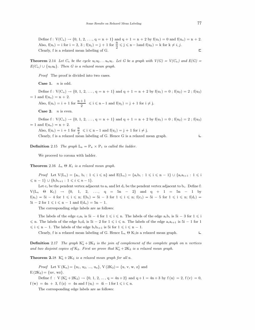
Some Results on Relaxed Mean Labeling 77
Define f : V(Cn) → {0, 1, 2, . . . , q = n + 1} and q + 1 = n + 2 by f(u1) = 0 and f(un) = n + 2.
Also, f(ui) = i for i = 2, 3 ; f(uj) = j + 1 forn
26 j 6 n− 1and f(uk) = k for k 6= i, j.
Clearly, f is a relaxed mean labeling of G. 2Theorem 2.14 Let Cn be the cycle u1u2. . . unu1. Let G be a graph with V(G) = V(Cn) and E(G) =
E(Cn) ∪ {u3u6}. Then G is a relaxed mean graph.
Proof The proof is divided into two cases.
Case 1. n is odd.
Define f : V(Cn) → {0, 1, 2, . . . , q = n + 1} and q + 1 = n + 2 by f(u1) = 0 ; f(u2) = 2 ; f(u3)
= 1 and f(un) = n + 2.
Also, f(ui) = i + 1 forn +1
26 i 6 n− 1 and f(uj) = j + 1 for i 6= j.
Case 2. n is even.
Define f : V(Cn) → {0, 1, 2, . . . , q = n + 1} and q + 1 = n + 2 by f(u1) = 0 ; f(u2) = 2 ; f(u3)
= 1 and f(un) = n + 2.
Also, f(ui) = i + 1 forn
26 i 6 n− 1 and f(uj) = j + 1 for i 6= j.
Clearly, f is a relaxed mean labeling of G. Hence G is a relaxed mean graph. 2Definition 2.15 The graph Ln = Pn × P1 is called the ladder.
We proceed to corona with ladder.
Theorem 2.16 Ln Θ K1 is a relaxed mean graph.
Proof Let V(Ln) = {ai, bi : 1 6 i 6 n} and E(Ln) = {aibi : 1 6 i 6 n − 1} ∪ {aiai+1 : 1 6 i
6 n − 1} ∪ {bibi+1 : 1 6 i 6 n − 1}.Let ci be the pendent vertex adjacent to ai and let di be the pendent vertex adjacent to bi. Define f:
V(Ln Θ K1) → {0, 1, 2, . . . , q = 5n − 2} and q + 1 = 5n − 1 by
f(ai) = 5i − 4 for 1 6 i 6 n; f(bi) = 5i − 3 for 1 6 i 6 n; f(ci) = 5i − 5 for 1 6 i 6 n; f(di) =
5i − 2 for 1 6 i 6 n − 1 and f(dn) = 5n − 1.
The corresponding edge labels are as follows:
The labels of the edge ciai is 5i − 4 for 1 6 i 6 n. The labels of the edge aibi is 5i − 3 for 1 6 i
6 n. The labels of the edge bidi is 5i − 2 for 1 6 i 6 n. The labels of the edge aiai+1 is 5i − 1 for 1
6 i 6 n − 1. The labels of the edge bibi+1 is 5i for 1 6 i 6 n − 1.
Clearly, f is a relaxed mean labeling of G. Hence Ln Θ K1is a relaxed mean graph. 2Definition 2.17 The graph Kc
n +2K2 is the join of complement of the complete graph on n vertices
and two disjoint copies of K2. First we prove that Kcn + 2K2 is a relaxed mean graph.
Theorem 2.18 Kcn +2K2 is a relaxed mean graph for all n.
Proof Let V (Kn) = {u1, u2, ..., un}, V (2K2)= {u, v, w, z} and
E (2K2)= {uv, wz}.Define f : V (Kc
n +2K2) → {0, 1, 2, ... , q = 4n +2} and q+ 1 = 4n + 3 by f (u) = 2, f (v) = 0,
f (w) = 4n + 3, f (z) = 4n and f (ui) = 4i − 1 for 1 6 i 6 n.
The corresponding edge labels are as follows:
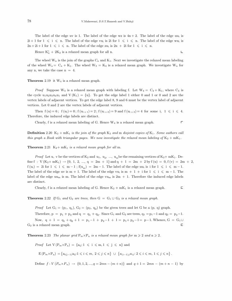
78 V.Maheswari, D.S.T.Ramesh and V.Balaji
The label of the edge uv is 1. The label of the edge wz is 4n + 2. The label of the edge uui is
2i + 1 for 1 6 i 6 n. The label of the edge vui is 2i for 1 6 i 6 n. The label of the edge wui is
2n +2i +1 for 1 6 i 6 n. The label of the edge zui is 2n + 2i for 1 6 i 6 n.
Hence Kcn + 2K2 is a relaxed mean graph for all n. 2
The wheel Wn is the join of the graphs Cn and K1. Next we investigate the relaxed mean labeling
of the wheel Wn = Cn + K1. The wheel W3 = K4 is a relaxed mean graph. We investigate Wn for
any n, we take the case n = 4.
Theorem 2.19 it W4 is a relaxed mean graph.
Proof Suppose W4 is a relaxed mean graph with labeling f. Let W4 = C4 + K1, where C4 is
the cycle u1u2u3u4u1 and V (K1) = {u}. To get the edge label 1 either 0 and 1 or 0 and 2 are the
vertex labels of adjacent vertices. To get the edge label 8, 9 and 6 must be the vertex label of adjacent
vertices. Let 0 and 2 are the vertex labels of adjacent vertices.
Then f (u)= 6 ; f (ui) = 0 ; f (ui + 1) = 2 ; f (ui + 2)= 9 and f (ui + 3) = 4 for some i, 1 6 i 6 4.
Therefore, the induced edge labels are distinct.
Clearly, f is a relaxed mean labeling of G. Hence W4 is a relaxed mean graph. 2Definition 2.20 K2 + mK1 is the join of the graph K2 and m disjoint copies of K1. Some authors call
this graph a Book with triangular pages. We now investigate the relaxed mean labeling of K2 + mK1.
Theorem 2.21 K2+ mK1 is a relaxed mean graph for all m.
Proof Let u, v be the vertices of K2 and u1, u2, ..., umbe the remaining vertices of K2+ mK1. De-
fine f : V (K2+ mK1) → {0, 1, 2, ..., q = 2m + 1} and q + 1 = 2m + 2 by f (u) = 0, f (v) = 2m + 2,
f (ui) = 2i for 1 6 i 6 m− 1 ; f(um) = 2m− 1. The label of the edge uui is i for 1 6 i 6 m− 1.
The label of the edge uv is m + 1. The label of the edge vui is m + 1 + i for 1 6 i 6 m − 1. The
label of the edge uum is m. The label of the edge vum is 2m + 1. Therefore the induced edge labels
are distinct.
Clearly, f is a relaxed mean labeling of G. Hence K2 + mK1 is a relaxed mean graph. 2Theorem 2.22 If G1 and G2 are trees, then G = G1 ∪ G2 is a relaxed mean graph.
Proof Let G1 = (p1, q1), G2 = (p2, q2) be the given trees and let G be a (p, q) graph.
Therefore, p = p1 + p2 and q = q1 + q2. Since G1 and G2 are trees, q1 =p1−1 and q2 = p2−1.
Now, q + 1 = q1 + q2 + 1 = p1−1 + p2−1 + 1 = p1+ p2−1= p−1. Whence, G = G1∪G2 is a relaxed mean graph. 2Theorem 2.23 The planar grid Pm×Pn is a relaxed mean graph for m > 2 and n > 2.
Proof Let V (Pm×Pn) = {aij: 1 6 i 6 m, 1 6 j 6 n} and
E (Pm×Pn) ={
ai(j−1)aij:1 6 i 6 m, 2 6 j 6 n}
∪{
a(i−1)jaij : 2 6 i 6 m, 1 6 j 6 n}
.
Define f : V (Pm×P n) → {0, 1, 2, ..., q = 2mn − (m + n)} and q + 1 = 2mn − (m + n − 1) by
Some Results on Relaxed Mean Labeling 79
f (a1j)= j − 1, 1 6 j 6 n and
f (aij) =
f(
a(i−1)n
)
+ (n − 1) + j, 2 6 i 6 m, 1 6 j 6 n.
f(
a(i−1)n
)
+ (n − 1) + j + 1 if m and n are maximum
The label of the edge aijai(j+1) is (i − 1) (2n − 1) +j for 1 6 i 6 m, 1 6 j 6 n − 1.
The label of the edge aija(i+1)j is (n − 1) + (i − 1) (2n − 1) + j for 1 6 i 6 m − 1,
1 6 j 6 n.
Clearly, f is a relaxed mean labeling of G Hence Pm×Pn is a relaxed mean graph for m > 2 and
n > 2. 2Theorem 2.24 The prism Pm×Cn is a relaxed mean graph for m > 2 and for all n > 3.
Proof Let V (Pm×Cn) = {aij : 1 6 i 6 m, 1 6 j 6 n} and
E (Pm×Cn) ={
ai (j−1) ai j : 1 6 i 6 m, 2 6 j 6 n}
⋃{
a(i−1) j aij : 2 6 i 6 m,1 6 j 6 n}
⋃ {ai1 ain: 1 6 i 6 m} .
Take
n =
2r if n is even
2r + 1 if n is odd
Define f : V (Pm×Cn) → {0, 1, 2, ..., q + 1 = (2mn − n) + 1} by f (a1j)= 2j
for 1 6 j 6 r and f (a1n) = 0, Also,
f (a1 r+j) =
n − 2j + 2 if n is odd for 1 6 j 6 r
n − 2j + 1 if n is even for 1 6 j 6 r − 1
f (a2j) = 2n + 2 (j − 1) for 1 6 j 6 r + 1
f (a2 r+1+j) =
3n − 2j + 2 if n is odd for 1 6 j 6 r
3n − 2j + 1 if n is even for 1 6 j 6 r − 1
f(
a(2i−1) j
)
= f (a1j) + 4n (i − 1) for 2 6 i 6m − 1
2, 1 6 j 6 n ;
Also, f(a(2i−1)1) = f(a11) + 5m for i =m + 1
2;
f(a(2i−1)2) = f(a12) + 5m + 2 for i =m + 1
2and f (a(2i−1)3) = f (a13) + 5m + 1 for i =
m + 1
2.
f(
a(2i−2) j
)
= f (a2j) + 4n (i − 2) for 3 6 i 6 m, 1 6 j 6 n.
Clearly, f is a relaxed mean labeling of Pm×Cn for m > 2, n > 3. Hence G is a relaxed mean
graph.
References
[1] J.A.Gallian, A dynamic survey of graph labeling, The Electronic Journal of Combinatorics, 16(2010),
# DS6.
[2] R.L.Graham and N.J.A. , On additive bases and harmonious graphs, SIAM J. Alg. Discrete
Math., 1 (1980) 382 – 404.
[3] F.Harary, Graph Theory, Addison-Wesley, Reading Mars., 1972.
80 V.Maheswari, D.S.T.Ramesh and V.Balaji
[4] V.Maheswari, D.S.T.Ramesh and V.Balaji, Relaxed mean labeling, International Journal of
Mathematics Research, Volume 4, 3 (2012), 217-224.
[5] Rosa, On certain valuation of the vertices of a graph, Theory of Graphs (International Symposium,
Rome, July 1966), Gorden and Breach, N.Y and Dunod Paris (1967) - 349 – 355.
[6] S.Somasundaram and R.Ponraj, Mean labeling of graphs, National Academic Science Letters,
26(2003), 210 – 213.
[7] S.Somasundaram and R.Ponraj, Some results on mean graphs, Pure and Applied Mathematika
Sciences, 58(2003), 29 – 35.
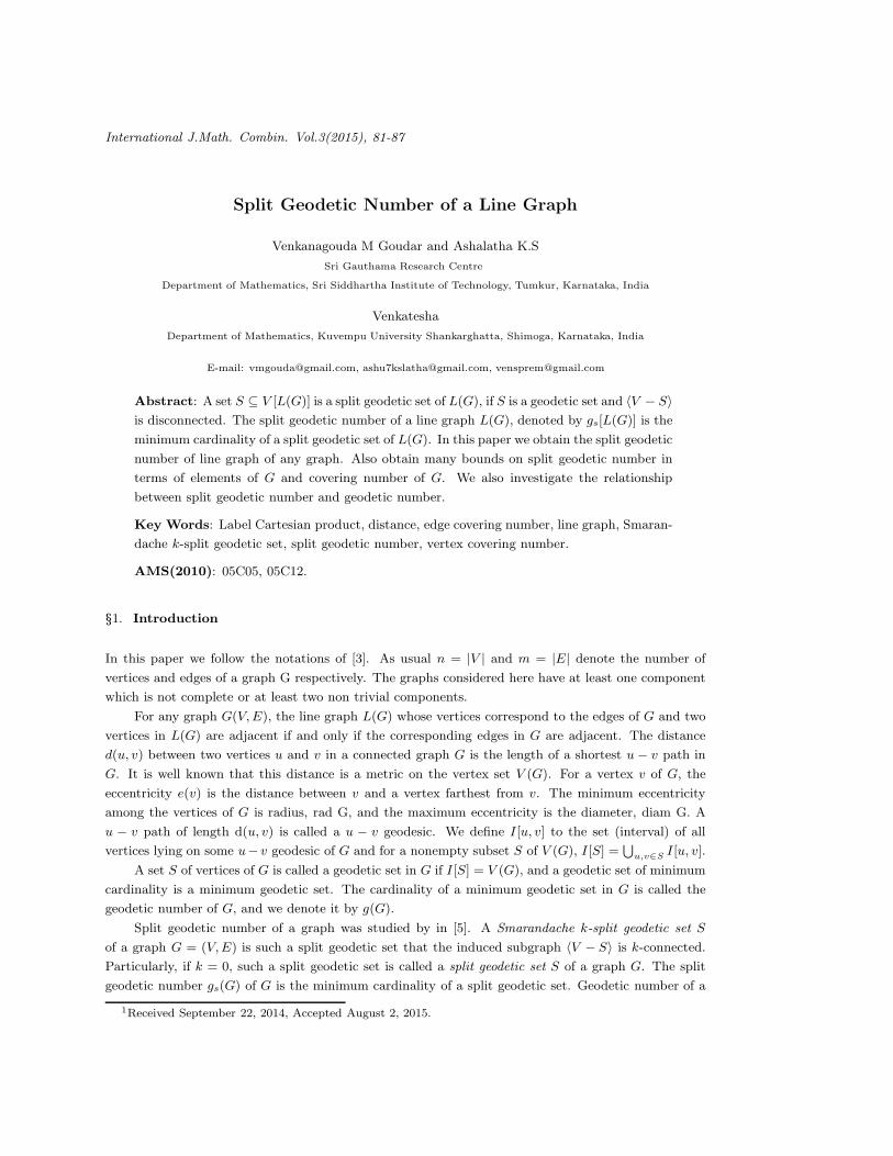
International J.Math. Combin. Vol.3(2015), 81-87
Split Geodetic Number of a Line Graph
Venkanagouda M Goudar and Ashalatha K.S
Sri Gauthama Research Centre
Department of Mathematics, Sri Siddhartha Institute of Technology, Tumkur, Karnataka, India
Venkatesha
Department of Mathematics, Kuvempu University Shankarghatta, Shimoga, Karnataka, India
E-mail: [email protected], [email protected], [email protected]
Abstract: A set S ⊆ V [L(G)] is a split geodetic set of L(G), if S is a geodetic set and 〈V − S〉is disconnected. The split geodetic number of a line graph L(G), denoted by gs[L(G)] is the
minimum cardinality of a split geodetic set of L(G). In this paper we obtain the split geodetic
number of line graph of any graph. Also obtain many bounds on split geodetic number in
terms of elements of G and covering number of G. We also investigate the relationship
between split geodetic number and geodetic number.
Key Words: Label Cartesian product, distance, edge covering number, line graph, Smaran-
dache k-split geodetic set, split geodetic number, vertex covering number.
AMS(2010): 05C05, 05C12.
§1. Introduction
In this paper we follow the notations of [3]. As usual n = |V | and m = |E| denote the number of
vertices and edges of a graph G respectively. The graphs considered here have at least one component
which is not complete or at least two non trivial components.
For any graph G(V, E), the line graph L(G) whose vertices correspond to the edges of G and two
vertices in L(G) are adjacent if and only if the corresponding edges in G are adjacent. The distance
d(u, v) between two vertices u and v in a connected graph G is the length of a shortest u − v path in
G. It is well known that this distance is a metric on the vertex set V (G). For a vertex v of G, the
eccentricity e(v) is the distance between v and a vertex farthest from v. The minimum eccentricity
among the vertices of G is radius, rad G, and the maximum eccentricity is the diameter, diam G. A
u − v path of length d(u, v) is called a u − v geodesic. We define I [u, v] to the set (interval) of all
vertices lying on some u− v geodesic of G and for a nonempty subset S of V (G), I [S] =⋃
u,v∈S I [u, v].
A set S of vertices of G is called a geodetic set in G if I [S] = V (G), and a geodetic set of minimum
cardinality is a minimum geodetic set. The cardinality of a minimum geodetic set in G is called the
geodetic number of G, and we denote it by g(G).
Split geodetic number of a graph was studied by in [5]. A Smarandache k-split geodetic set S
of a graph G = (V, E) is such a split geodetic set that the induced subgraph 〈V − S〉 is k-connected.
Particularly, if k = 0, such a split geodetic set is called a split geodetic set S of a graph G. The split
geodetic number gs(G) of G is the minimum cardinality of a split geodetic set. Geodetic number of a
1Received September 22, 2014, Accepted August 2, 2015.
82 Venkanagouda M Goudar, Ashalatha K.S and Venkatesha
line graph was studied by in [4]. Geodetic number of a line graph L(G) of G is a set S′
of vertices of
L(G) = H is called the geodetic set in H if I(S′
) = V (H) and a geodetic set of minimum cardinality is
the geodetic number of L(G) and is denoted by g[L(G)]. Now we define split geodetic number of a line
graph. A set S′
of vertices of L(G) = H is called the split geodetic set in H if the induced subgraph
V (H)−S′
is disconnected and a split geodetic set of minimum cardinality is the split geodetic number
of L(G) and is denoted by gs[L(G)].
A vertex v is an extreme vertex in a graph G, if the subgraph induced by its neighbors is complete.
A vertex cover in a graph G is a set of vertices that covers all edges of G. The minimum number of
vertices in a vertex cover of G is the vertex covering number α0(G) of G. An edge cover of a graph
G without isolated vertices is a set of edges of G that covers all the vertices of G. The edge covering
number α1(G) of a graph G is the minimum cardinality of an edge cover of G.
For terminologies and notations not mentioned here, we follow references [2] and [3].
§2. Preliminary Notes
We need results following for proving results in this paper.
Theorem 2.1([1]) Every geodetic set of a graph contains its extreme vertices.
Theorem 2.2([5]) For cycle Cn of order n > 3,
gs(Cn) =
2 if n is even
3 if n is odd.
Theorem 2.3([1]) Let G be a connected graph of order at least 3. If G contains a minimum geodetic
set S with a vertex x such that every vertex of G lies on some x − w geodesic in G for some w ∈ S,
then g(G) = g(G × K2).
Proposition 2.4 For any graph G, g(G) ≤ gs(G).
Proposition 2.5 For any tree T of order n and number of cut vertices ci then the number of end edges
is n − ci.
§3. Main Results
Theorem 3.1 For any tree T with k end edges and ci be the number of cut vertices, having more than
three internal vertices, gs[L(T )] = n − ci + 1.
Proof Let S be the set of all extreme vertices of a line graph L(T ) of a tree T . Let vi be a cut
vertex in V − S and S′
= S ∪ {vi}. By Theorem 2.1, gs[L(T )] ≥ |S′ |. On the other hand, for an
internal vertex v of L(T ), there exists x, y of L(T ) such that v lies on a unique x− y geodesic in L(T ).
The corresponding end edges of T are the extreme vertices of L(T ) and the induced subgraph V −S′
is
disconnected. Thus gs[L(T )] ≤ |S′ |. Also, every split geodetic set S1 of L(T ) must contain S′
which is
the unique minimum split geodetic set. Thus |S′ | = |S1| = k +1. By Proposition 2.5, |S1| = n− ci +1.
Hence, gs[L(T )] = n − ci + 1. 2
Split Geodetic Number of a Line Graph 83
Corollary 3.2 For any path Pn, n ≥ 6, gs[L(Pn)] = 3.
Proof Clearly, the set of two end vertices of a path Pn is its unique geodetic set. From Theorem
3.1, the results follows. 2Proposition 3.3 Line graph of a cycle is again a cycle of same order.
Theorem 3.4 For cycle Cn of order n > 3,
gs[L(Cn)] =
2 if n is even
3 if n is odd.
Proof The result follows from Proposition 3.3 and Theorem 2.2. 2Theorem 3.5 For the wheel Wn = K1 + Cn−1 (n ≥ 6),
gs[L(Wn)] =
n
2+ 2 if n is even
n + 1
2+ 2 if n is odd.
Proof Let Wn = K1+Cn−1(n ≥ 6) and let V (Wn) = {x, v1, v2, · · · , vn−1}, where deg(x) = n−1 >
3 and deg(vi) = 3 for each i ∈ {1, 2, · · · , n − 1}. Now U = {u1, u2, · · · , uj} are the vertices of L(Wn)
formed from edges of Cn−1, i.e., U ⊆ V [L(Wn)] and Y = {y1, y2, · · · , yj} are the vertices of L(Wn)
formed from internal edges of Wn. Thus, Y ⊆ V [L(Wn)]. We consider the following cases.
Case 1. n is even.
Let H ⊆ U . Now S = H ∪{yj} forms a minimum geodetic set of L(Wn). Let P = {p1, p2, · · · , pi}be the vertices of V [L(Wn)] − S. Clearly, S ∪ {pl, pk} forms a minimum split geodetic set of L(Wn)
and |S ∪ {pl, pk}| =n
2+ 2. Therefore, gs[L(Wn)] =
n
2+ 2.
Case 2. n is odd.
Let H ⊆ U , now S = H ∪ {yj , yj−1} forms a minimum geodetic set of L(Wn). Let P =
{p1, p2, · · · , pi} be the vertices of V [L(Wn)]− S. Now S ∪ {pl, pk} forms a minimum split geodetic set
of L(Wn). Clearly, |S ∪ {pl, pk}| =n + 1
2+ 2. Therefore, gs[L(Wn)] =
n + 1
2+ 2. 2
As an immediate consequence of the above theorem we have the following.
Corollary 3.6 For the wheel Wn = K1 + Cn−1 (n ≥ 6),
gs[L(Wn)] =
∆ + δ
2if n is even
∆ + δ + 1
2if n is odd.
Proof Minimum degree(δ) of L(Wn) is equal to 4 and maximum degree(∆) of L(Wn) is equal to
n. i,e number of vertices in Wn.
Case 1. n is even.
84 Venkanagouda M Goudar, Ashalatha K.S and Venkatesha
We have known from Case 1 of Theorem 3.5 that
gs[L(Wn)] =n
2+ 2
gs[L(Wn)] =n + 4
2
gs[L(Wn)] =∆ + δ + 1
2
Case 2. n is odd.
We have known from Case 2 of Theorem 3.5 that
gs[L(Wn)] =n + 1
2+ 2
gs[L(Wn)] =n + 4 + 1
2
gs[L(Wn)] =∆ + δ + 1
2. 2
Theorem 3.7 For the wheel Wn = K1 + Cn−1 (n ≥ 6), gs[L(Wn)] + g[L(Wn)] ≤ m.
Proof Let U = {u1, u2, · · · , uj} ⊆ V [L(Wn)] be the set of vertices formed from edges of Cn−1 and
Y = {y1, y2, · · · , yj} ⊆ V [L(Wn) be the set of vertices formed from internal edges of Wn. Consider S =
H∪{yj}, where H ⊂ U forms a minimum geodetic set of L(Wn). Furthermore, if P = {p1, p2, · · · , pi} is
the set of vertices of V [L(Wn)]−S, then S′
= S∪{pl, pm} forms a minimum split geodetic set of L(Wn).
Notice that V [L(G)] = E(G) = m. It follows that |S′ | ∪ |S| ≤ m. Thus, gs[L(Wn)] + g[L(Wn)] ≤ m.2Theorem 3.8 For a tree T with more than three internal vertices, gs[L(T )] ≥ m − α1 + 1, where α1
is the edge covering number.
Proof Suppose S = {e1, e2, · · · , ek} to be the set of all end edges in T . Then S ∪ J , where
J ⊆ E(T )− S is the minimal set of edges which covers all the vertices of T such that |S ∪ J | = α1(T ).
Without loss of generality, let I = {u1, u2, · · · , un} ⊆ V [L(T )] be the set of vertices in L(T ) formed by
the end edges in T . Suppose H = {u1, u2, · · · , ui} ⊆ V [L(T )] − I . Then I ∪ {ui} forms a minimum
split geodetic set of L(T ), where each ui ∈ H with deg ≥ 2. Clearly, it follows that |I ∪ {ui}| ≥|E(T )| − |S ∪ J | + 1. Therefore, gs[L(T )] ≥ m − α1(T ) + 1. 2Theorem 3.9 If every non end vertex of a tree T with more than three internal vertex is adjacent to
at least one end vertex, then gs[L(T )] ≥ n − k, where k is the number of end vertices in T .
Proof Let S′
= {v1, v2, · · · , vk} be the set of all end vertices in T with |S′ | = k. Without loss
of generality, let every end edge of T be the extreme vertices of L(T ). Suppose L(T ) does not contain
any end vertex. Then S = I ∪ {uj}, where I = {u1, u2, · · · , ui} ⊆ V [L(T )] and uj ∈ V [L(T )] − I with
deg ≥ 2 forms a minimum split geodetic set of L(T ). Furthermore, if L(T ) contain at least one end
vertex vi, then the set S ∪ {vi} forms a minimum split geodetic set of L(T ). Therefore, we obtain
|S ∪ {vi}| ≥ n − |S′ |. Clearly it follows that gs[L(T )] ≥ n − k. 2Theorem 3.10 For any connected graph G of order n, gs(G) + gs[L(G)] ≤ 2n.
Proof Let S = {v1, v2, · · · , vn} ⊆ V (G) be the minimum split geodetic set of G. Now without
loss of generality, if F = {u1, u2, · · · , uk} is the set of all end vertices in L(G), then F ∪ H , where
H ⊆ V [L(G)]− F forms a minimum split geodetic set of L(G). Since each vertex in L(G) corresponds
Split Geodetic Number of a Line Graph 85
to two adjacent vertices of G, it follows that |S| ∪ |F ∪ H | ≤ 2n. Therefore gs(G) + gs[L(G)] ≤ 2n. 2Theorem 3.11 Let G be a connected graph of order n with diameter d > 4. Then gs[L(G)] ≤ n−d+2.
Proof Let u and v be vertices of L(G) for which d(u, v) = d and let u = v0, v1, · · · , vd = v
be the u − v path of length d. Now let S = V [L(G)] − {v1, v2, · · · , vd−1}. Then I(S) = V [L(G)],
V [L(G)] − (S ∪ {v2}) is disconnected and gs[L(G)] ≤ |S| = n − d + 2. 2Theorem 3.12 For any integers r, s ≥ 2, gs[L(Kr,s)] ≤ rs.
Proof Notice that the diameter of L(Kr,s) is 2 and the number of vertices in L(Kr,s) is rs. By
Theorem 3.11, gs[L(G)] ≤ n−d+2. Now we have gs[L(Kr,s)] ≤ rs−2+2. Therefore, gs[L(Kr,s)] ≤ rs.2Theorem 3.13 For any integer n ≥ 4, gs[L(Kn)] ≤ n(n − 1)
2.
Proof Let n ≥ 4 be the vertices of the given graph Kn with diameter d. Since diameter of L(Kn)
is 2 and the number of vertices in L(Kn) isn(n − 1)
2. By Theorem 3.11, gs[L(G)] ≤ n − d + 2. We
have
gs[L(Kn)] ≤ n(n − 1)
2− 2 + 2 ⇒ gs[L(Kn)] ≤ n(n − 1)
2. 2
Theorem 3.14 For any cycle Cn with n ≡ 0(mod2), gs[L(Cn)] =n
α0(Cn), where α0 is the vertex
covering number.
Proof Let n > 3 be number of vertices which is even and let α0 be the vertex covering number
of Cn. By Theorem 3.4, gs[L(Cn)] = 2. Also, for even cycle, the vertex covering number α0(Cn) =n
2.
Hence gs[L(Cn)] = 2 =n
n/2=
n
α0(Cn). 2
Theorem 3.15 For any cycle Cn with n ≡ 1(mod2), gs[L(Cn)] =n + 1
α0(Cn)+ 1, where α0 is the vertex
covering number.
Proof Let n > 3 be the number of vertices which is odd and let α0 be the vertex covering number
of Cn. By Theorem 3.4, gs[L(Cn)] = 3. Also, for odd cycle, vertex covering number α0(Cn) =n + 1
2.
Hence gs[L(Cn)] = 2 + 1 =n + 1
α0(Cn)+ 1. 2
§4. Adding an End Edge
For an edge e = (u, v) of a graph G with deg(u) = 1 and deg(v) > 1, we call e an end-edge and u an
end-vertex.
Theorem 4.1 Let G′
be the graph obtained by adding k end edges {(u, v1), (u, v2), · · · , (u, vk)} to a
cycle Cn = G of order n > 3, with u ∈ G and {v1, v2, · · · , vk} /∈ G. Then gs[L(G′
)] = k + 2.
Proof Let {e1, e2, · · · , en, e1} be edges on a cycle of order n and let G′
be the graph obtained
from G = Cn by adding end edges (u, vi), i = 1, 2, · · · , k such that u ∈ G but vi /∈ G.
86 Venkanagouda M Goudar, Ashalatha K.S and Venkatesha
Case 1. n is even.
By definition, L(G′
) has 〈Kk+2〉 as an induced subgraph. Also the edges (u, vi), i = 1, 2, · · · , k
becomes vertices of L(G′
) and it belongs to some geodetic set of L(G′
). Hence {e1, e2, · · · , ek, el, em}are the vertices of L(G
′
), where el, em are the edges incident on the antipodal vertex of u in G′
and these
vertices belongs to some geodetic set of L(G′
). L(G′
) = Cn ∪ Kk+2. LetS = {e1, e2, · · · , ek, el, em} be
the geodetic set. Suppose P = {e1, e2, · · · , ek} is the set of vertices of L(G′
) such that |P | < |S|. Then,
P is not a geodetic set of L(G′
). Clearly, S is the minimum geodetic set. Since V − S is disconnected
S is the minimum split geodetic set. Therefore gs[L(C2n)] = k + 2.
Case 2. n is odd.
By definition, L(G′
) has 〈Kk+2〉 as an induced subgraph, also the edges (u, vi) = {e1, e2, · · · , ek}becomes vertices of L(G
′
). Let el = (a, b) ∈ G such that d(u, a) = d(u, b) in the graph L(G′
). and let
S = {e1, e2, · · · , ek, el} be the geodetic set. Now S′
= S ∪ {em} is a split geodetic set, where em is
the vertex from V − S with deg ≥ 2. It is clear that S′
is the minimum split geodetic set. Therefore
gs[L(C2n+1)] = k + 2. 2Theorem 4.2 Let G
′
be the graph obtained by adding end edge (ui, vj), i = 1, 2, · · · , n, j = 1, 2, · · · , k
to each vertex of G = Cn of order n > 3 such that ui ∈ G, vj /∈ G. Then gs[L(G′
)] = k + 2.
Proof Let {e1, e2, · · · , en, e1} be edges on a cycle G = Cn and let G′
be the graph obtained by
adding end edge (ui, vj), i = 1, 2, · · · , n, j = 1, 2, · · · , k to each vertex of G such that ui ∈ G but vj /∈ G.
Clearly, k be the number of end vertices of G′
. By definition, L(G′
) have n copies of K3 as an induced
subgraph. The edges (ui, vj) = ej for all j becomes k vertices of L(G′
) and those lies on geodetic set of
L(G′
). They form the extreme vertices of L(G′
). By Theorem 2.1 S = {e1, e2, · · · , ek} forms a geodetic
set. Now consider any two vertices {el, em} ∈ V −S which are not adjacent. S′
= {e1, e2, · · · , ek, el, em}forms a split geodetic set of L(G
′
). Suppose P = {e1, e2, · · · , ek, el} is the set of vertices of L(G′
) such
that |P | < |S′ |. Then, V − P is connected. Hence it is clear that S′
is the minimum split geodetic set
of L(G′
). There fore gs[L(G′
)] = k + 2. 2§5. Cartesian Product
The Cartesian product of the graphs H1 and H2, written as H1 × H2, is the graph with vertex set
V (H1) × V (H2), two vertices u1, u2 and v1, v2 being adjacent in H1 × H2 if and only if either u1 = v1
and (u2, v2) ∈ E(H2), or u2 = v2 and (u1, v1) ∈ E(H1).
Theorem 5.1 For any path Pn of order n,
gs[L(K2 × Pn)] =
2 for n = 2
3 for n = 3
4 for n > 3.
Proof Let K2 ×Pn be formed from two copies of G1 and G2 of Pn. Now, L(K2 ×Pn) formed from
two copies of G′
1, G′
2 of L(Pn). And let U = {u1, u2, · · · , un−1} ∈ V (G′
1), W = {w1, w2, · · · , wn−1} ∈V (G
′
2). We have the following cases.
Split Geodetic Number of a Line Graph 87
Case 1. If n = 2, by the definition L(K2 × P2) = K2 × P2. By Theorem 2.3,
gs[L(K2 × P2)] = g[L(K2 × P2)] = g(P2) = 2.
Case 2. If n = 3, L(K2 × P3) is formed from two copies of P2. Clearly, gs[L(K2 × P3)] = 3.
Case 3. If n > 3, let S be the split geodetic set of L(K2 × Pn). We claim that S contains
two elements (end vertices) from each set {u1, un−1, w1, wn−1} and V − S is disconnected. Since
I(S) = V [L(K2 × Pn)], it follows that gs[L(K2 × Pn)] ≤ 4. It remains to show that if S′
is a three
element subset of V [L(K2 × Pn)], then I(S′
) 6= V [L(K2 × Pn)]. First assume that S′
is a subset U or
W , say the former. Then I(S′
) = S′ ∪ W 6= V . Therefore, we may take that S
′ ∩ U = {ui, uj} and
S′ ∩ W = {wk}. Then
I(S′
) = {ui, uj} ∪ W 6= V [L(K2 × Pn)]. 2References
[1] G.Chartrand, F.Harary and P.Zhang, On the geodetic number of a graph, Networks, 39(2002),
1-6.
[2] G.Chartrand and P.Zhang, Introduction to Graph Theory, Tata McGraw Hill Pub.Co. Ltd., 2006.
[3] F.Harary, Graph Theory, Addison-Wesely, Reading, MA, 1969.
[4] Venkanagouda M.Goudar, K.S.Ashalatha, Venkatesha and M.H.Muddebihal, On the geodetic
number of line graph, Int.J.Contemp.Math.Sciences, Vol.7, No.46(2012), 2289-2295.
[5] Venkanagouda M.Goudar, K.S.Ashalatha and Venkatesha, Split geodetic number of a graph, Ad-
vances and Applications in Discrete Mathematics, Vol.13, No.1(2014), 9-22.
International J.Math. Combin. Vol.3(2015), 88-98
Skolem Difference Odd Mean Labeling For Some Simple Graphs
R.Vasuki, J.Venkateswari and G.Pooranam
Department of Mathematics, Dr.Sivanthi Aditanar College of Engineering
Tiruchendur- 628 215, Tamilnadu, India
E-mail: [email protected], [email protected], [email protected]
Abstract: A graph G with p vertices and q edges is said to have skolem difference odd mean
labeling if there exists an injective function f : V (G) → {1, 2, 3, · · · , 4q − 1} such that the
induced map f∗ : E(G) → {1, 3, 5, · · · , 2q − 1} defined by
f∗(uv) =
|f(u) − f(v)|2
if |f(u) − f(v)| is even
|f(u) − f(v)| + 1
2if |f(u) − f(v)| is odd
is a bijection. A graph that admits skolem difference odd mean labeling is called a skolem
difference odd mean graph. Here we investigate skolem difference odd mean behaviour of
some standard graphs.
Key Words: Labeling, skolem difference odd mean graph, Smarandache k-mean graph.
AMS(2010): 05C78.
§1. Introduction
Throughout this paper, by a graph we mean a finite, undirected and simple graph. Let G(V, E) be a
graph with p vertices and q edges. For notations and terminology we follow [1].
Path on n vertices is denoted by Pn and a cycle on n vertices is denoted by Cn. A graph G = (V, E)
is called bipartite if V = V1 ∪ V2 with φ = V1 ∩ V2, and every edge of G is of the form {u, v} with
u ∈ V1 and v ∈ V2. If each vertex in V1 is joined with every vertex in V2, we have a complete bipartite
graph. In this case |V1| = m and |V2| = n, the graph is denoted by Km,n. The complete bipartite graph
K1,n is called a star graph and it is denoted by Sm. The bistar Bm,n is the graph obtained from K2 by
identifying the center vertices of K1,m and K1,n at the end vertices of K2 respectively. Bm,m is often
denoted by B(m).
A quadrilateral snake Qn is obtained from a path u1, u2, · · · , un+1 by joining ui and ui+1 to new
vertices vi and wi respectively and joining vi and wi, 1 ≤ i ≤ n, that is, every edge of a path is replaced
by a cycle C4. The corona of a graph G on p vertices v1, v2, · · · , vp is the graph obtained from G by
adding p new vertices u1, u2, · · · , up and the new edges uivi for 1 ≤ i ≤ p. The corona of G is denoted by
G⊙K1. The graph Pn ⊙K1 is called a comb. Let G1 and G2 be any two graphs with p1 and p2 vertices
respectively. Then the cartesian product G1 ×G2 has p1p2 vertices which are {(u, v)/u ∈ G1, v ∈ G2}.The edge set of G1 × G2 is obtained as follows: (u1, v1) and (u2, v2) are adjacent in G1 × G2 if either
1Received March 24, 2014, Accepted May 15, 2015.
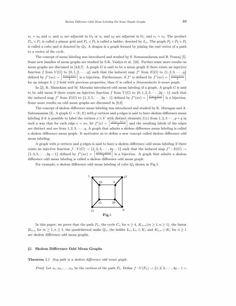
Skolem Difference Odd Mean Labeling For Some Simple Graphs 89
u1 = u2 and v1 and v2 are adjacent in G2 or u1 and u2 are adjacent in G1 and v1 = v2. The product
Pm ×Pn is called a planar grid and Pn ×P2 is called a ladder, denoted by Ln. The graph P2 ×P2 ×P2
is called a cube and is denoted by Q3. A dragon is a graph formed by joining the end vertex of a path
to a vertex of the cycle.
The concept of mean labeling was introduced and studied by S. Somasundaram and R. Ponraj [5].
Some new families of mean graphs are studied by S.K. Vaidya et al. [10]. Further some more results on
mean graphs are discussed in [4,6,7]. A graph G is said to be a mean graph if there exists an injective
function f from V (G) to {0, 1, 2, · · · , q} such that the induced map f∗ from E(G) to {1, 2, 3, · · · , q}defined by f∗(uv) =
⌈
f(u)+f(v)2
⌉
is a bijection. Furthermore, if f∗ is defined by f∗(uv) =⌈
f(u)+f(v)k
⌉
for an integer k ≥ 2 hold with previous properties, then G is called a Smarandache k-mean graph.
In [2], K. Manickam and M. Marudai introduced odd mean labeling of a graph. A graph G is said
to be odd mean if there exists an injective function f from V (G) to {0, 1, 2, 3, · · · , 2q − 1} such that
the induced map f∗ from E(G) to {1, 3, 5, · · · , 2q − 1} defined by f∗(uv) =⌈
f(u)+f(v)2
⌉
is a bijection.
Some more results on odd mean graphs are discussed in [8,9].
The concept of skolem difference mean labeling was introduced and studied by K. Murugan and A.
Subramanian [3]. A graph G = (V, E) with p vertices and q edges is said to have skolem difference mean
labeling if it is possible to label the vertices x ∈ V with distinct elements f(x) from 1, 2, 3 · · · , p + q in
such a way that for each edge e = uv, let f∗(e) =⌈
|f(u)−f(v)|2
⌉
and the resulting labels of the edges
are distinct and are from 1, 2, 3, · · · , q. A graph that admits a skolem difference mean labeling is called
a skolem difference mean graph. It motivates us to define a new concept called skolem difference odd
mean labeling.
A graph with p vertices and q edges is said to have a skolem difference odd mean labeling if there
exists an injective function f : V (G) → {1, 2, 3, · · · , 4q − 1} such that the induced map f∗ : E(G) →{1, 3, 5, · · · , 2q − 1} defined by f∗(uv) =
⌈
|f(u)−f(v)|2
⌉
is a bijection. A graph that admits a skolem
difference odd mean labeling is called a skolem difference odd mean graph.
For example, a skolem difference odd mean labeling of cube Q3 shown in Fig.1.
1 47
15 9
13 39
23 5
Fig.1
In this paper, we prove that the path Pn, the cycle Cn for n ≥ 4, Km,n(m ≥ 1, n ≥ 1), the bistar
Bm,n for m ≥ 1, n ≥ 1, the quadrilateral snake Qn, the ladder Ln, Ln ⊙ K1 and K1,n ⊙ K1 for n ≥ 1
are skolem difference odd mean graphs.
§2. Skolem Difference Odd Mean Graphs
Theorem 2.1 Any path is a skolem difference odd mean graph.
Proof Let u1, u2, . . . , un be the vertices of the path Pn. Define f : V (Pn) → {1, 2, 3, · · · , 4q − 1 =
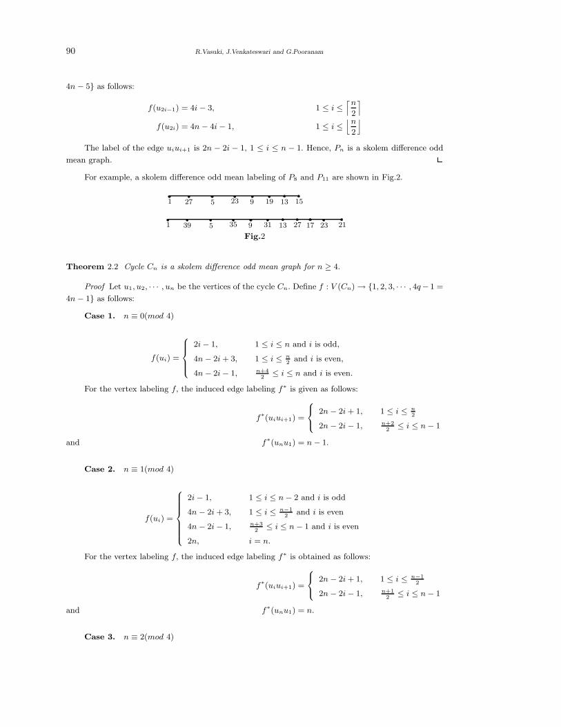
90 R.Vasuki, J.Venkateswari and G.Pooranam
4n − 5} as follows:
f(u2i−1) = 4i − 3, 1 ≤ i ≤⌈n
2
⌉
f(u2i) = 4n − 4i − 1, 1 ≤ i ≤⌊n
2
⌋
The label of the edge uiui+1 is 2n − 2i − 1, 1 ≤ i ≤ n − 1. Hence, Pn is a skolem difference odd
mean graph. 2For example, a skolem difference odd mean labeling of P8 and P11 are shown in Fig.2.
1 39 5 35 9 31 13 27 17 23 21
1 27 5 23 9 19 13 15
Fig.2
Theorem 2.2 Cycle Cn is a skolem difference odd mean graph for n ≥ 4.
Proof Let u1, u2, · · · , un be the vertices of the cycle Cn. Define f : V (Cn) → {1, 2, 3, · · · , 4q− 1 =
4n − 1} as follows:
Case 1. n ≡ 0(mod 4)
f(ui) =
2i − 1, 1 ≤ i ≤ n and i is odd,
4n − 2i + 3, 1 ≤ i ≤ n2
and i is even,
4n − 2i − 1, n+42
≤ i ≤ n and i is even.
For the vertex labeling f, the induced edge labeling f∗ is given as follows:
f∗(uiui+1) =
2n − 2i + 1, 1 ≤ i ≤ n2
2n − 2i − 1, n+22
≤ i ≤ n − 1
and f∗(unu1) = n − 1.
Case 2. n ≡ 1(mod 4)
f(ui) =
2i − 1, 1 ≤ i ≤ n − 2 and i is odd
4n − 2i + 3, 1 ≤ i ≤ n−12
and i is even
4n − 2i − 1, n+32
≤ i ≤ n − 1 and i is even
2n, i = n.
For the vertex labeling f, the induced edge labeling f∗ is obtained as follows:
f∗(uiui+1) =
2n − 2i + 1, 1 ≤ i ≤ n−12
2n − 2i − 1, n+12
≤ i ≤ n − 1
and f∗(unu1) = n.
Case 3. n ≡ 2(mod 4)
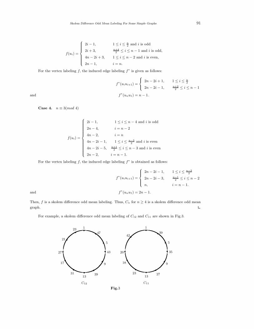
Skolem Difference Odd Mean Labeling For Some Simple Graphs 91
f(ui) =
2i − 1, 1 ≤ i ≤ n2
and i is odd
2i + 3, n+42
≤ i ≤ n − 1 and i is odd,
4n − 2i + 3, 1 ≤ i ≤ n − 2 and i is even,
2n − 1, i = n.
For the vertex labeling f, the induced edge labeling f∗ is given as follows:
f∗(uiui+1) =
2n − 2i + 1, 1 ≤ i ≤ n2
2n − 2i − 1, n+22
≤ i ≤ n − 1
and f∗(unu1) = n − 1.
Case 4. n ≡ 3(mod 4)
f(ui) =
2i − 1, 1 ≤ i ≤ n − 4 and i is odd
2n − 4, i = n − 2
4n − 2, i = n
4n − 2i − 1, 1 ≤ i ≤ n−32
and i is even
4n − 2i − 5, n+12
≤ i ≤ n − 3 and i is even
2n − 2, i = n − 1.
For the vertex labeling f, the induced edge labeling f∗ is obtained as follows:
f∗(uiui+1) =
2n − 2i − 1, 1 ≤ i ≤ n−32
2n − 2i − 3, n−12
≤ i ≤ n − 2
n, i = n − 1.
and f∗(unu1) = 2n − 1.
Then, f is a skolem difference odd mean labeling. Thus, Cn for n ≥ 4 is a skolem difference odd mean
graph. 2For example, a skolem difference odd mean labeling of C12 and C11 are shown in Fig.3.
1
47
5
43
9
3913
31
17
27
21
23
C12
1
39
5
35
9
2713
23
18
20
C11
42
Fig.3
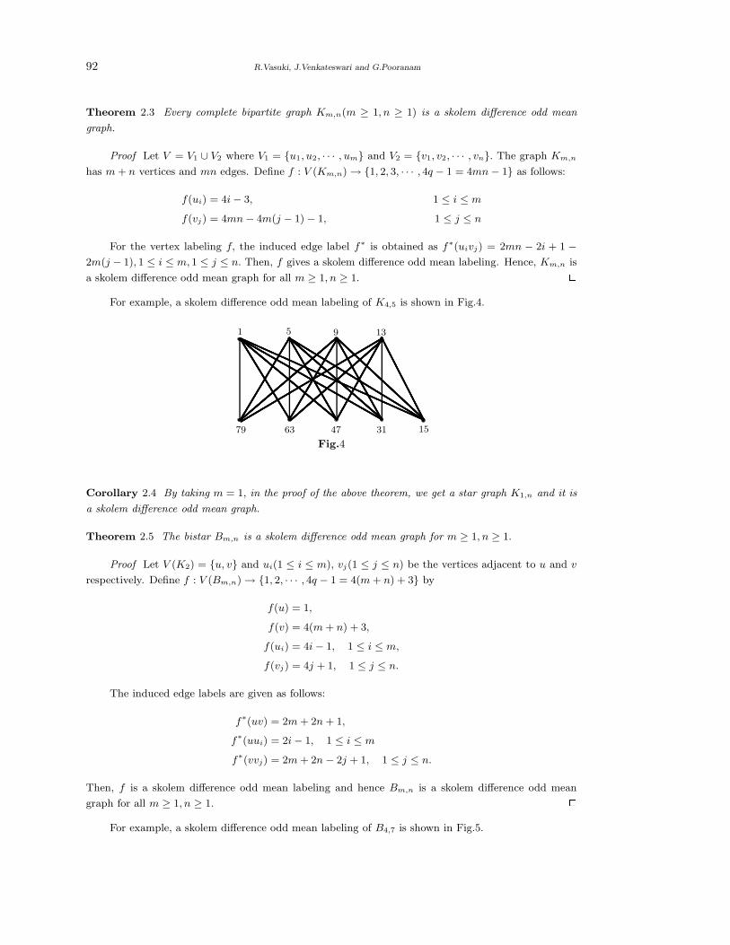
92 R.Vasuki, J.Venkateswari and G.Pooranam
Theorem 2.3 Every complete bipartite graph Km,n(m ≥ 1, n ≥ 1) is a skolem difference odd mean
graph.
Proof Let V = V1 ∪ V2 where V1 = {u1, u2, · · · , um} and V2 = {v1, v2, · · · , vn}. The graph Km,n
has m + n vertices and mn edges. Define f : V (Km,n) → {1, 2, 3, · · · , 4q − 1 = 4mn − 1} as follows:
f(ui) = 4i − 3, 1 ≤ i ≤ m
f(vj) = 4mn − 4m(j − 1) − 1, 1 ≤ j ≤ n
For the vertex labeling f, the induced edge label f∗ is obtained as f∗(uivj) = 2mn − 2i + 1 −2m(j − 1), 1 ≤ i ≤ m, 1 ≤ j ≤ n. Then, f gives a skolem difference odd mean labeling. Hence, Km,n is
a skolem difference odd mean graph for all m ≥ 1, n ≥ 1. 2For example, a skolem difference odd mean labeling of K4,5 is shown in Fig.4.
1 5 9 13
79 63 47 31 15
Fig.4
Corollary 2.4 By taking m = 1, in the proof of the above theorem, we get a star graph K1,n and it is
a skolem difference odd mean graph.
Theorem 2.5 The bistar Bm,n is a skolem difference odd mean graph for m ≥ 1, n ≥ 1.
Proof Let V (K2) = {u, v} and ui(1 ≤ i ≤ m), vj(1 ≤ j ≤ n) be the vertices adjacent to u and v
respectively. Define f : V (Bm,n) → {1, 2, · · · , 4q − 1 = 4(m + n) + 3} by
f(u) = 1,
f(v) = 4(m + n) + 3,
f(ui) = 4i − 1, 1 ≤ i ≤ m,
f(vj) = 4j + 1, 1 ≤ j ≤ n.
The induced edge labels are given as follows:
f∗(uv) = 2m + 2n + 1,
f∗(uui) = 2i − 1, 1 ≤ i ≤ m
f∗(vvj) = 2m + 2n − 2j + 1, 1 ≤ j ≤ n.
Then, f is a skolem difference odd mean labeling and hence Bm,n is a skolem difference odd mean
graph for all m ≥ 1, n ≥ 1. 2For example, a skolem difference odd mean labeling of B4,7 is shown in Fig.5.
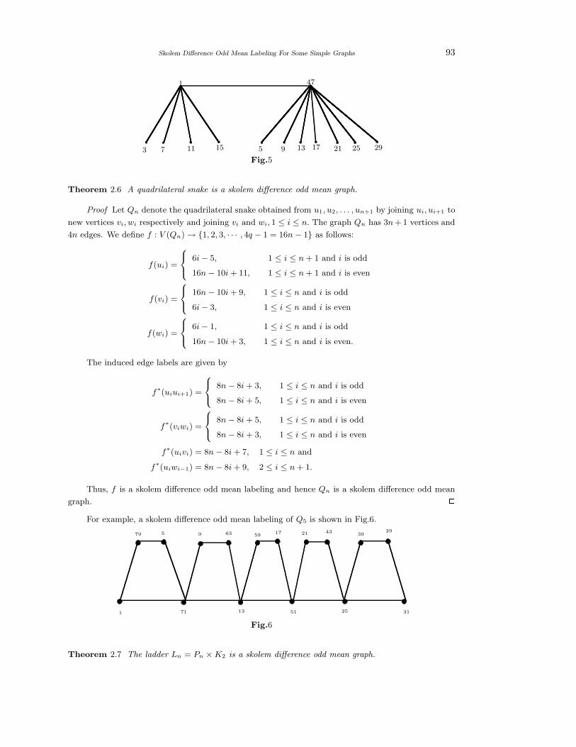
Skolem Difference Odd Mean Labeling For Some Simple Graphs 93
1 47
3 7 11 15 5 9 13 17 21 25 29
Fig.5
Theorem 2.6 A quadrilateral snake is a skolem difference odd mean graph.
Proof Let Qn denote the quadrilateral snake obtained from u1, u2, . . . , un+1 by joining ui, ui+1 to
new vertices vi, wi respectively and joining vi and wi, 1 ≤ i ≤ n. The graph Qn has 3n + 1 vertices and
4n edges. We define f : V (Qn) → {1, 2, 3, · · · , 4q − 1 = 16n − 1} as follows:
f(ui) =
6i − 5, 1 ≤ i ≤ n + 1 and i is odd
16n − 10i + 11, 1 ≤ i ≤ n + 1 and i is even
f(vi) =
16n − 10i + 9, 1 ≤ i ≤ n and i is odd
6i − 3, 1 ≤ i ≤ n and i is even
f(wi) =
6i − 1, 1 ≤ i ≤ n and i is odd
16n − 10i + 3, 1 ≤ i ≤ n and i is even.
The induced edge labels are given by
f∗(uiui+1) =
8n − 8i + 3, 1 ≤ i ≤ n and i is odd
8n − 8i + 5, 1 ≤ i ≤ n and i is even
f∗(viwi) =
8n − 8i + 5, 1 ≤ i ≤ n and i is odd
8n − 8i + 3, 1 ≤ i ≤ n and i is even
f∗(uivi) = 8n − 8i + 7, 1 ≤ i ≤ n and
f∗(uiwi−1) = 8n − 8i + 9, 2 ≤ i ≤ n + 1.
Thus, f is a skolem difference odd mean labeling and hence Qn is a skolem difference odd mean
graph. 2For example, a skolem difference odd mean labeling of Q5 is shown in Fig.6.
1 71 13 51 25 31
79 5 9 63 5917 21 43
3929
Fig.6
Theorem 2.7 The ladder Ln = Pn × K2 is a skolem difference odd mean graph.
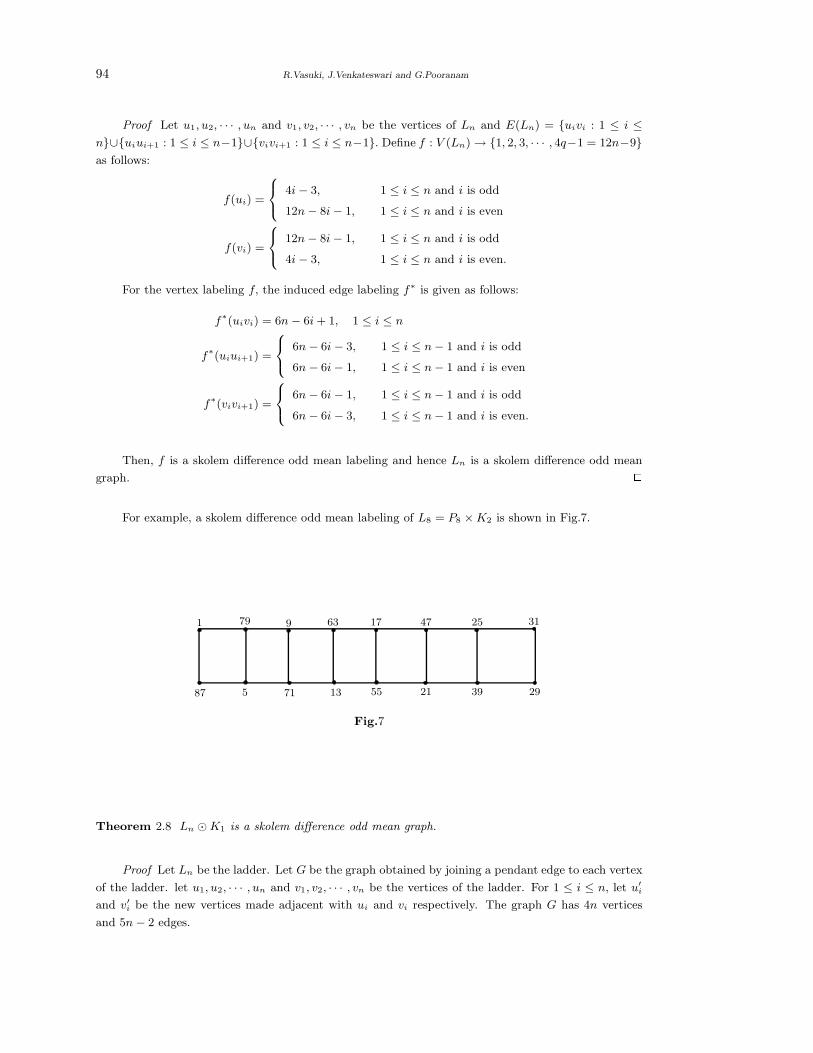
94 R.Vasuki, J.Venkateswari and G.Pooranam
Proof Let u1, u2, · · · , un and v1, v2, · · · , vn be the vertices of Ln and E(Ln) = {uivi : 1 ≤ i ≤n}∪{uiui+1 : 1 ≤ i ≤ n−1}∪{vivi+1 : 1 ≤ i ≤ n−1}. Define f : V (Ln) → {1, 2, 3, · · · , 4q−1 = 12n−9}as follows:
f(ui) =
4i − 3, 1 ≤ i ≤ n and i is odd
12n − 8i − 1, 1 ≤ i ≤ n and i is even
f(vi) =
12n − 8i − 1, 1 ≤ i ≤ n and i is odd
4i − 3, 1 ≤ i ≤ n and i is even.
For the vertex labeling f, the induced edge labeling f∗ is given as follows:
f∗(uivi) = 6n − 6i + 1, 1 ≤ i ≤ n
f∗(uiui+1) =
6n − 6i − 3, 1 ≤ i ≤ n − 1 and i is odd
6n − 6i − 1, 1 ≤ i ≤ n − 1 and i is even
f∗(vivi+1) =
6n − 6i − 1, 1 ≤ i ≤ n − 1 and i is odd
6n − 6i − 3, 1 ≤ i ≤ n − 1 and i is even.
Then, f is a skolem difference odd mean labeling and hence Ln is a skolem difference odd mean
graph. 2For example, a skolem difference odd mean labeling of L8 = P8 × K2 is shown in Fig.7.
1 79 9 63 17 47 25 31
87 5 71 13 55 21 39 29
Fig.7
Theorem 2.8 Ln ⊙ K1 is a skolem difference odd mean graph.
Proof Let Ln be the ladder. Let G be the graph obtained by joining a pendant edge to each vertex
of the ladder. let u1, u2, · · · , un and v1, v2, · · · , vn be the vertices of the ladder. For 1 ≤ i ≤ n, let u′i
and v′i be the new vertices made adjacent with ui and vi respectively. The graph G has 4n vertices
and 5n − 2 edges.
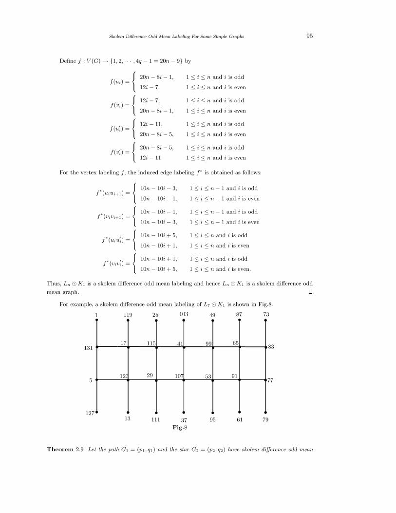
Skolem Difference Odd Mean Labeling For Some Simple Graphs 95
Define f : V (G) → {1, 2, · · · , 4q − 1 = 20n − 9} by
f(ui) =
20n − 8i − 1, 1 ≤ i ≤ n and i is odd
12i − 7, 1 ≤ i ≤ n and i is even
f(vi) =
12i − 7, 1 ≤ i ≤ n and i is odd
20n − 8i − 1, 1 ≤ i ≤ n and i is even
f(u′i) =
12i − 11, 1 ≤ i ≤ n and i is odd
20n − 8i − 5, 1 ≤ i ≤ n and i is even
f(v′i) =
20n − 8i − 5, 1 ≤ i ≤ n and i is odd
12i − 11 1 ≤ i ≤ n and i is even
For the vertex labeling f, the induced edge labeling f∗ is obtained as follows:
f∗(uiui+1) =
10n − 10i − 3, 1 ≤ i ≤ n − 1 and i is odd
10n − 10i − 1, 1 ≤ i ≤ n − 1 and i is even
f∗(vivi+1) =
10n − 10i − 1, 1 ≤ i ≤ n − 1 and i is odd
10n − 10i − 3, 1 ≤ i ≤ n − 1 and i is even
f∗(uiu′i) =
10n − 10i + 5, 1 ≤ i ≤ n and i is odd
10n − 10i + 1, 1 ≤ i ≤ n and i is even
f∗(viv′i) =
10n − 10i + 1, 1 ≤ i ≤ n and i is odd
10n − 10i + 5, 1 ≤ i ≤ n and i is even.
Thus, Ln ⊙K1 is a skolem difference odd mean labeling and hence Ln ⊙K1 is a skolem difference odd
mean graph. 2For example, a skolem difference odd mean labeling of L7 ⊙ K1 is shown in Fig.8.
1 119 25 103 49 87 73
131
5
127
17
123
13
115
29
111
41
107
37
99
53
95
65
91
61
83
77
79
Fig.8
Theorem 2.9 Let the path G1 = (p1, q1) and the star G2 = (p2, q2) have skolem difference odd mean
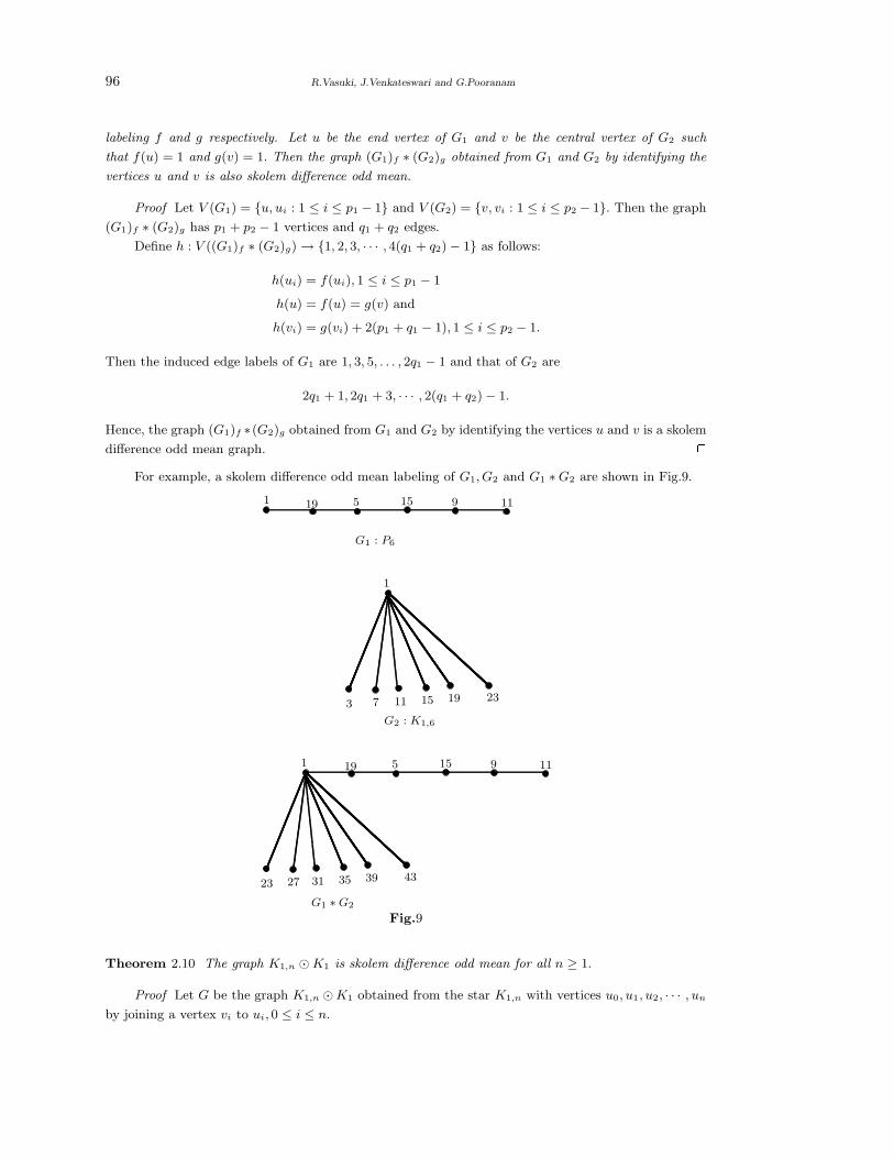
96 R.Vasuki, J.Venkateswari and G.Pooranam
labeling f and g respectively. Let u be the end vertex of G1 and v be the central vertex of G2 such
that f(u) = 1 and g(v) = 1. Then the graph (G1)f ∗ (G2)g obtained from G1 and G2 by identifying the
vertices u and v is also skolem difference odd mean.
Proof Let V (G1) = {u, ui : 1 ≤ i ≤ p1 − 1} and V (G2) = {v, vi : 1 ≤ i ≤ p2 − 1}. Then the graph
(G1)f ∗ (G2)g has p1 + p2 − 1 vertices and q1 + q2 edges.
Define h : V ((G1)f ∗ (G2)g) → {1, 2, 3, · · · , 4(q1 + q2) − 1} as follows:
h(ui) = f(ui), 1 ≤ i ≤ p1 − 1
h(u) = f(u) = g(v) and
h(vi) = g(vi) + 2(p1 + q1 − 1), 1 ≤ i ≤ p2 − 1.
Then the induced edge labels of G1 are 1, 3, 5, . . . , 2q1 − 1 and that of G2 are
2q1 + 1, 2q1 + 3, · · · , 2(q1 + q2) − 1.
Hence, the graph (G1)f ∗(G2)g obtained from G1 and G2 by identifying the vertices u and v is a skolem
difference odd mean graph. 2For example, a skolem difference odd mean labeling of G1, G2 and G1 ∗ G2 are shown in Fig.9.
1
23 27 31 35 39 43
19 5 15 9 11
G1 ∗ G2
G1 : P6
1 19 5 15 9 11
1
3 7 11 15 19 23
G2 : K1,6
Fig.9
Theorem 2.10 The graph K1,n ⊙ K1 is skolem difference odd mean for all n ≥ 1.
Proof Let G be the graph K1,n ⊙K1 obtained from the star K1,n with vertices u0, u1, u2, · · · , un
by joining a vertex vi to ui, 0 ≤ i ≤ n.
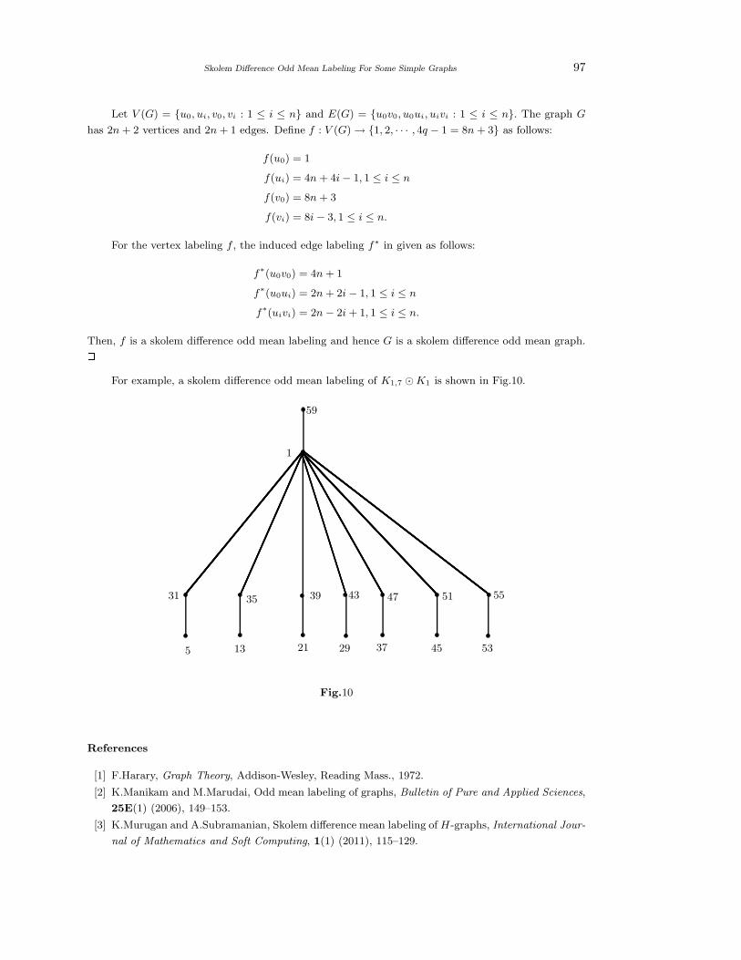
Skolem Difference Odd Mean Labeling For Some Simple Graphs 97
Let V (G) = {u0, ui, v0, vi : 1 ≤ i ≤ n} and E(G) = {u0v0, u0ui, uivi : 1 ≤ i ≤ n}. The graph G
has 2n + 2 vertices and 2n + 1 edges. Define f : V (G) → {1, 2, · · · , 4q − 1 = 8n + 3} as follows:
f(u0) = 1
f(ui) = 4n + 4i − 1, 1 ≤ i ≤ n
f(v0) = 8n + 3
f(vi) = 8i − 3, 1 ≤ i ≤ n.
For the vertex labeling f , the induced edge labeling f∗ in given as follows:
f∗(u0v0) = 4n + 1
f∗(u0ui) = 2n + 2i − 1, 1 ≤ i ≤ n
f∗(uivi) = 2n − 2i + 1, 1 ≤ i ≤ n.
Then, f is a skolem difference odd mean labeling and hence G is a skolem difference odd mean graph.2For example, a skolem difference odd mean labeling of K1,7 ⊙ K1 is shown in Fig.10.
59
1
31 35 39 43 47 51 55
5 13 21 29 37 45 53
Fig.10
References
[1] F.Harary, Graph Theory, Addison-Wesley, Reading Mass., 1972.
[2] K.Manikam and M.Marudai, Odd mean labeling of graphs, Bulletin of Pure and Applied Sciences,
25E(1) (2006), 149–153.
[3] K.Murugan and A.Subramanian, Skolem difference mean labeling of H-graphs, International Jour-
nal of Mathematics and Soft Computing, 1(1) (2011), 115–129.
98 R.Vasuki, J.Venkateswari and G.Pooranam
[4] A.Nagarajan and R.Vasuki, On the meanness of arbitrary path super subdivision of paths, Aus-
tralian J. Combin., 51 (2011), 41–48.
[5] S.Somasundaram and R.Ponraj, Mean labelings of graphs, National Academy Science Letters, 26
(2003), 210–213.
[6] R.Vasuki and A.Nagarajan, Meanness of the graphs Pa,b and P ba , International Journal of Applied
Mathematics, 22(4) (2009), 663–675.
[7] R.Vasuki and S.Arokiaraj, On mean graphs, International Journal of Mathematical Combinatorics,
3 (2013), 22–34.
[8] R.Vasuki and A.Nagarajan, Odd mean labeling of the graphs Pa,b, Pba and P b
〈2a〉, Kragujevac
Journal of Mathematics, 36(1) (2012), 125–134.
[9] R.Vasuki and S.Arokiaraj, On odd mean graphs, Journal of Discrete Mathematical Sciences and
Cryptography, (To appear).
[10] S.K.Vaidya and Lekha Bijukumar, Some new families of mean graphs, Journal of Mathematics
Research, 2(3) (2010), 169–176.
International J.Math. Combin. Vol.3(2015), 99-104
Radio Number for Special Family of Graphs with
Diameter 2, 3 and 4
M.Murugan
(School of Science, Tamil Nadu Open University, 577, Anna Salai, Chennai - 600 015, India)
E-mail: [email protected]
Abstract: A radio labeling of a graph G is an injective function [4] f : V (G) → N ∪ {0}such that for every u, v ∈ V (G),
|f(u) − f(v)| > diam(G) − d(u, v) + 1.
The span of f is the difference of the largest and the smallest channels used, that is,
maxu,v∈V (G)
{f(u) − f(v)}.
The radio number of G is defined as the minimum span of a radio labeling of G and denoted
as rn(G). In this paper, we present algorithms to get the radio labeling of special family
of graphs like double cones, books and nC4 with a common vertex whose diameters are 2,3
and 4 respectively.
Key Words: Radio labeling, radio number, channel assignment, distance two labeling.
AMS(2010): 05C78, 05C12, 05C15.
§1. Introduction
The channel assignment problem is a telecommunication problem in which our aim is to assign a
channel (non-negative integer) to each TV or Radio station so that we do not have any interference
in the communication. The level of interference between the TV or Radio stations correlates with the
geographic locations of these stations. Earlier designers of TV networks considered close locations and
very close locations so that the transmitters at the close locations receive different channels and the
transmitters at very close locations are at least two apart for clear communication.
This can be modeled by graph models in which vertices represent the stations and two vertices
are joined by an edge if they are very close and they are joined by a path of length 2 if they are close.
The mathematical abstraction of the above concept is distance two labeling or L(2, 1)-labeling. A
L(2, 1)-labeling of a graph G is an assignment f from the vertex set V (G) to the set of non-negative
integers such that |f(x) − f(y)| > 2 if x and y are adjacent and |f(x) − f(y)| > 1 if x and y are at
distance 2, for all x and y in V (G).
Practically speaking the interference among channels may go beyond two levels. So we have to
1Received October 12, 2014, Accepted August 25, 2015.
100 M.Murugan
extend the interference level from two to the largest possible - the diameter of the corresponding graph.
So the concept of L(2, 1) labeling was generalized to radio labeling.
Radio labeling was originally introduced by G.Chartrand et.al., [1] in 2001. A radio labeling of a
graph G is an injective function f : V (G) → N ∪ {0} such that for every u, v ∈ V (G),
|f(u) − f(v)| > diam(G) − d(u, v) + 1.
The span of f is the difference of the largest and the smallest channels used, that is,
maxu,v∈V (G)
{f(u) − f(v)}.
The radio number of G is defined as the minimum span of a radio labeling of G and denoted as rn(G).
§2. Some Existing Results
(1) D.D.F. Liu and X. Zhu [2] have discussed the radio number for paths and cycles.
(2) D.D.F. Liu [3] has obtained lower bounds for the radio number of trees and characterized trees
achieving this bound.
(3) Mustapha et al. [4] have discussed radio k-labeling for cartesian products of graphs.
(4) The radio labeling of cube and fourth power of cycles have been discussed by B. Sooryanarayana
and P. Raghunath [5, 6].
(5) The radio labeling of kth power of a path is discussed by P. Devadas Rao et al. [7]
(6) The radio number for the split graph and the middle graph of cycle Cn is discussed by S.K.
Vaidya et al. [8].
In the survey of literature available on radio labeling, we found that only two types of problems
are considered in this area till this date.
(1) To investigate bounds for the radio number of a graph;
(2) To completely determine the radio number of a graph.
§3. Results
In this section, we develop and justify algorithms to get Radio labeling of the family of graphs - double
cones whose diameter is 2, books whose diameter is 3 and nC4 with a common vertex whose diameter
is 4.
We note that the concept of radio labeling and L(2, 1) labeling coincides when the diameter of the
graph is 2. In general, to prove a labeling is a radio labeling, we have to prove that every u, v ∈ V (G),
|f(u) − f(v)| > diam(G) − d(u, v) + 1.
Double Cones are graphs obtained by joining two isolated vertices to every vertex of Cn. A Double
Cone on n + 2 vertices is denoted by COn+2 = Cn + 2K1. We note that COn+2 has two vertices with
maximum degree n.
Algorithm 1:
Input : A double cone COn+2 = Cn + 2K1, n > 5.
Output : Radio labeling of COn+2.
Radio Number for Special Family of Graphs with Diameter 2, 3 and 4 101
Step 1: Arrange the vertices of Cn as v1, v2, . . . , vn and let u1, u2 denotes 2K1.
Step 2: First label vis of odd i and then label vis of even i starting from the label 3 and ending
with n + 2 consecutively.
Step 3 : Label u1 with 0 and u2 with 1.
The justification of the desired output is proved in Theorem 3.1.
Theorem 3.1 For the double cone COn+2, n > 5, rn(COn+2) = n + 2.
Proof Consider the double cone COn+2, n > 5. Let V (Cn) = {v1, v2, . . . , vn} and u1, u2 denotes
2K1. Define f : V (COn+2) → N ∪ {0} such that
f(u1) = 0
f(u2) = 1
f(v1) = 3
f(vi) = f(v1) +i − 1
2if i is odd and i > 1.
f(v2) = f(v1) +⌈n
2
⌉
f(vi) = f(v1) +⌈n
2
⌉
+i − 2
2if i is even and i > 2.
When d(vi, vj) = 1, we have |f(vi) − f(vj)| =⌈
n2
⌉
or⌈
n2
⌉
− 1, n − 1. That is, when d(vi, vj) = 1, we
have |f(vi) − f(vj)| > 2. When d(vi, vj) = 2, we have |f(vi) − f(vj)| > 1 since f(vi)s are distinct.
Since f(vi) > 3 and f(u1) = 0, we have |f(vi) − f(u1)| > 3. Since f(vi) > 3 and f(u2) = 1, we have
|f(vi) − f(u2)| > 2. Hence f is a radio labeling and rn(COn+1) 6 n + 2.
Since COn+2 has two vertices u1 and u2 with maximum degree n and that too, they are adjacent
with the same vertices v1, v2, . . . , vn, the consecutive n + 2 labels 0, 1, 2, . . . , n + 1 are not sufficient to
produce a radio-labeling. Therefore, rn(COn+2) > n + 2 and hence rn(COn+2) = n + 2. 2A book Bn is the product of the star K1,n with K2. A book Bn has p = 2n+2 vertices, q = 3n+1
edges, n pages, maximum degree n + 1 and diameter 3. Next we present an algorithm to get a radio
labeling of a book Bn.
Algorithm 2:
Input : A book Bn, n > 4, with p vertices.
Output : Radio labeling of Bn.
Step 1: Let the vertices of the nth page of Bn be v, vn, wn and w where v and w lie on the
common edge vw.
Step 2: Label v with the label p + 1 and w with the label 0.
Step 3: Label vi with 2i, i = 1, 2, · · · , n.
Step 4: Label wi with f(vi) + 5, i = 1, 2, . . . , n − 2 and wn−1 with the label 3 and wn with the
label 5, where f(vi) is the label of vi.
The justification of the desired output is proved in Theorem 3.2.
Theorem 3.2 For a Book Bn, n > 4, rn(Bn) = p + 1.
102 M.Murugan
Proof Consider a book Bn. A book Bn has p = 2n + 2 vertices, q = 3n + 1 edges, n pages,
maximum degree n + 1 and diameter 3. Let the vertices of the nth page of Bn be v, vn, wn and w
where v and w lie on the common edge vw.
Define f : V (Bn) → N ∪ {0} such that
f(v) = p + 1
f(w) = 0
f(vi) = 2i, i = 1, 2, · · · , n
f(wi) = f(vi) + 5, i = 1, 2, · · · , n − 2
f(wn−1) = 3
f(wn) = 5
We note that d(v, vi) = 1, d(w, wi) = 1, d(vi, wi) = 1, i = 1, 2, . . . , n and d(v, w) = 1. Now,
|f(v) − f(vi)| = p + 1 − 2i = 2n + 2 + 1 − 2i = 2n + 3 − 2i > 3, i = 1, 2, · · · , n.
|f(w) − f(wi)| = f(vi) + 5 = 2i + 5 > 3, i = 1, 2, · · · , n − 2.
|f(w) − f(wn−1)| = 3.
|f(w) − f(wn)| = 5.
Consider f(vi) − f(wi) = 2i + 5 − 2i = 5, i = 1, 2, · · · , n − 2.
|f(vn−1) − f(wn−1)| = 2n − 2 − 3 = 2n − 5 > 3.
|f(vn) − f(wn)| = 2n − 5 > 3.
Also |f(v) − f(w)| = p + 1 = 2n + 3.
Thus, |f(si) − f(ti)| > 3 when d(si, ti) = 1, si, ti ∈ V (Bn). We note that d(v, wi) = 2, d(w, vi) = 2,
i = 1, 2, · · · , n, d(vi, vj) = 2, i 6= j, i, j = 1, 2, · · · , n and d(wi, wj) = 2, i 6= j, i, j = 1, 2, · · · , n.
When d(v, wi) = 2, i = 1, 2, · · · , n,
|f(v) − f(wi)| = p + 1 − 2i − 5 = 2n + 2 + 1 − 2i − 5 = 2n − 2 − 2i > 2,
i = 1, 2, · · · , n − 2.
|f(v) − f(wn−1)| = p + 1 − 3 = p − 2 > 2
|f(v) − f(wn)| = p + 1 − 5 = p − 4 > 2
When d(w, vi) = 2, i = 1, 2, · · · , n, |f(w) − f(vi)| = 2i > 2, i = 1, 2, · · · , n. When d(vi, vj) = 2,
i 6= j, i, j = 1, 2, · · · , n, consider for i > j, |f(vi) − f(vj)| = 2i − 2j > 2. When d(wi, wj) = 2,
i 6= j, i, j = 1, 2, · · · , n − 2, consider for i > j, |f(wi) − f(wj)| = |f(vi) − f(vj)| = 2i − 2j > 2. Since
f(wn−1) = 3 and f(wn) = 5, |f(wi) − f(wj)| > 2, for all i, j = 1, 2, · · · , n. Thus, |f(si) − f(ti)| > 2
when d(si, ti) = 2, si, ti ∈ V (Bn).
Since all the vertex labels are distinct, we have,
|f(si) − f(ti)| > 1 when d(si, ti) = 3, si, ti ∈ V (Bn).
Hence f is a radio labeling and rn(Bn) 6 p + 1.
Since there are p vertices, there should be p distinct labels. The p labels 0, 1, 2, · · · , p − 1 are not
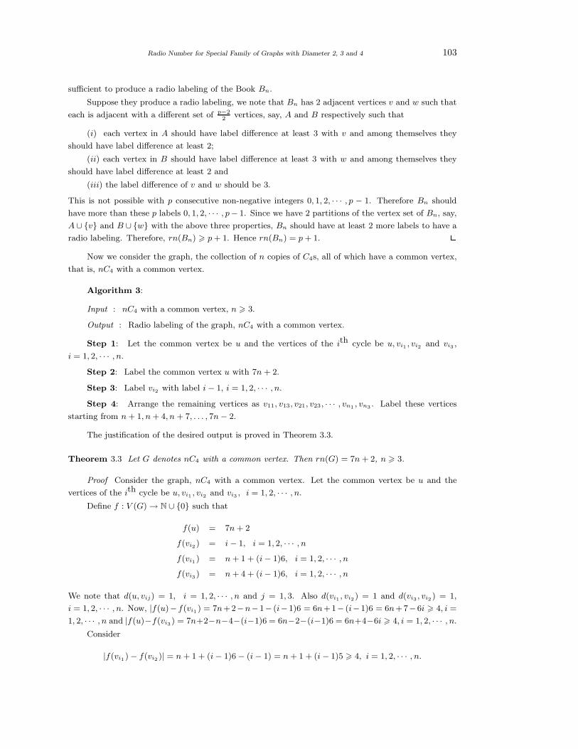
Radio Number for Special Family of Graphs with Diameter 2, 3 and 4 103
sufficient to produce a radio labeling of the Book Bn.
Suppose they produce a radio labeling, we note that Bn has 2 adjacent vertices v and w such that
each is adjacent with a different set of p−22
vertices, say, A and B respectively such that
(i) each vertex in A should have label difference at least 3 with v and among themselves they
should have label difference at least 2;
(ii) each vertex in B should have label difference at least 3 with w and among themselves they
should have label difference at least 2 and
(iii) the label difference of v and w should be 3.
This is not possible with p consecutive non-negative integers 0, 1, 2, · · · , p − 1. Therefore Bn should
have more than these p labels 0, 1, 2, · · · , p− 1. Since we have 2 partitions of the vertex set of Bn, say,
A ∪ {v} and B ∪ {w} with the above three properties, Bn should have at least 2 more labels to have a
radio labeling. Therefore, rn(Bn) > p + 1. Hence rn(Bn) = p + 1. 2Now we consider the graph, the collection of n copies of C4s, all of which have a common vertex,
that is, nC4 with a common vertex.
Algorithm 3:
Input : nC4 with a common vertex, n > 3.
Output : Radio labeling of the graph, nC4 with a common vertex.
Step 1: Let the common vertex be u and the vertices of the ith cycle be u, vi1 , vi2 and vi3 ,
i = 1, 2, · · · , n.
Step 2: Label the common vertex u with 7n + 2.
Step 3: Label vi2 with label i − 1, i = 1, 2, · · · , n.
Step 4: Arrange the remaining vertices as v11, v13, v21, v23, · · · , vn1 , vn3 . Label these vertices
starting from n + 1, n + 4, n + 7, . . . , 7n − 2.
The justification of the desired output is proved in Theorem 3.3.
Theorem 3.3 Let G denotes nC4 with a common vertex. Then rn(G) = 7n + 2, n > 3.
Proof Consider the graph, nC4 with a common vertex. Let the common vertex be u and the
vertices of the ith cycle be u, vi1 , vi2 and vi3 , i = 1, 2, · · · , n.
Define f : V (G) → N ∪ {0} such that
f(u) = 7n + 2
f(vi2 ) = i − 1, i = 1, 2, · · · , n
f(vi1 ) = n + 1 + (i − 1)6, i = 1, 2, · · · , n
f(vi3 ) = n + 4 + (i − 1)6, i = 1, 2, · · · , n
We note that d(u, vij) = 1, i = 1, 2, · · · , n and j = 1, 3. Also d(vi1 , vi2) = 1 and d(vi3 , vi2 ) = 1,
i = 1, 2, · · · , n. Now, |f(u)− f(vi1 ) = 7n+2−n−1− (i−1)6 = 6n+1− (i−1)6 = 6n+7−6i > 4, i =
1, 2, · · · , n and |f(u)−f(vi3) = 7n+2−n−4−(i−1)6 = 6n−2−(i−1)6 = 6n+4−6i > 4, i = 1, 2, · · · , n.
Consider
|f(vi1 ) − f(vi2 )| = n + 1 + (i − 1)6 − (i − 1) = n + 1 + (i − 1)5 > 4, i = 1, 2, · · · , n.
104 M.Murugan
Consider
|f(vi3 ) − f(vi2 )| = n + 4 + (i − 1)6 − (i − 1) = n + 4 + (i − 1)5 > 4, i = 1, 2, · · · , n.
We note that, for i = 1, 2, . . . , n and j = 2, d(u, vij) = 2 and for i, α = 1, 2, · · · , n and j, k = 1, 3,
d(vij , vαk) = 2 (i, α, j, k all are not equal).
Since f(u) = 7n + 2 and for i = 1, 2, · · · , n and j = 2, f(vij) = i − 1, we have,
|f(u) − f(vij)| = 7n + 2 − i + 1 = 7n + 3 − i > 3, i = 1, 2, · · · , n and j = 2.
Now, since, for i = 1, 2, · · · , n, f(vi1) = n + 1 + (i − 1)6 and f(vi3 ) = n + 4 + (i − 1)6, we have,
for i, α = 1, 2, · · · , n and j, k = 1, 3, (i, α, j, k all are not equal), |f(vij) − f(vαk) > 3.
Next, we note that, for i = 1, 2, · · · , n, d(vi2 , vjk) = 3 where j = 1, 2, · · · , n & j 6= i and k = 1, 3. In
this case, |f(vj1 ) − f(vi2 ) = n + 1 + (j − 1)6 − (i − 1) = n + 6j − i − 4 > 2. Also, |f(vj3 ) − f(vi2)| =
n + 4 + (j − 1)6− (i− 1) = n + 6j − i− 1 > 2. Finally, for i 6= j, d(vi2 , vj2) = 4. Since all the labels of
vi2 , i = 1, 2, · · · , n are distinct, |f(vi2 ) − f(vj2)| > 1. Hence f is a radio labeling and rn(G) 6 7n + 2.
Now we find the optimal value of rn(G). The minimum possible label of u is 0. Since the
distance between u and v11 is 1, the minimum label we can use at v11 is at least 4. Since the vertices
v13, v21, v23, v31, v33, · · · , vn1 , vn3 are at a distance 2 from v11, each of this should have a label difference
3 with v11 and among themselves. And so the minimum range of the labels for these vertices is
{7, 10, · · · , 6n+1}. So, without loss of generality,we assume that the minimum label vn3 should receive
is 6n+1. There are n more vertices, namely, v12, v22, · · · , vn2 . We cannot use the label 6n+2 to any of
these vertices because these vertices are at a distance 3 from vn3 and hence the label difference at these
vertices should be at least 2. So the minimum label we can use to any one of these vertices is 6n + 3
and there are n such vertices. Therefore the minimum label we required to label all these vertices is
6n + 1 + (n + 1) = 7n + 2.
Therefore, the minimum label which can give a radio labeling for the graph G is 7n + 2. That is,
rn(G) > 7n + 2. Hence, rn(G) = 7n + 2. 2References
[1] Gary Chartrand, David Erwin, Frank Harary and Phing Zhang, Radio labelings of graphs, Bulletin
of Inst. Combin. Appl., 33, (2001), 77-85.
[2] Daphne Der-Fen Liu and Xuding Zhu, Multilevel distance labelings for paths cycles, SIAM J.
Discrete Math., 19, (2005), 610-621.
[3] Daphne Der-Fen Liu, Radio number for trees, Discrete Mathematics, 308, (7), (2007), 1153-1164.
[4] Mustapha Kchilkech, Riadh Khennoufs and Olivier Togni, Radio k-Labelings for Cartesian Prod-
ucts of Graphs, Discussiones Mathematicae Graph Theory, 28(1) (2008), 165-178.
[5] B.Sooryanarayana and P.Raghunath, On the radio labeling of cube of a cycle, Far East J. Appl.
Math., 29 (1), (2007), 113-147.
[6] B.Sooryanarayana and P.Raghunath, On the radio labeling of fourth power of a cycle, Journal of
Applied Mathematical Analysis and Applications, 3(2), (2007), 195-228.
[7] P.Devadas Rao, B.Sooryanarayana and Chandru Hegde, On the radio labeling of kth power of a
path, Journal of Graphs and Combinatorics , Submitted.
[8] S.K.Vaidya and P.L.Vihol, Radio labeling for some cycle related graphs, International Journal of
Mathematics and Soft Computing, Vol.2. No.2 (2012), 11-24.
International J.Math. Combin. Vol.3(2015), 105-115
Vertex-to-Edge-set Distance Neighborhood Pattern Matrices
Kishori P.Narayankar and Lokesh S. B.
(Department of Mathematics, Mangalore University, Mangalagangothri-574 199, India)
Veena Mathad
(Department of Studies in Mathematics, University of Mysore, Manasagangothri-570 006, India)
E-mail: kishori [email protected], [email protected], veena [email protected]
Abstract: The vertex to edge set (VTES) distance d1(u, e) from a vertex u ∈ V (G) to
an edge e ∈ E(G) is the number of edges on (u − e) path. For each u ∈ V (G) define
NMj [u] = {e ∈ M ⊆ V (G) : d(u, e) = j, where 0 ≤ j ≤ d1(G) } and a non-negative integer
matrix DM1 (G) = (|NM
j [u]|) of order V (G) × ((d1(G) + 1) called the VTES-M-distance
neighborhood pattern (M-dnp) matrix of G. If fM : u 7−→ fM (u) is an injective function,
where fM (u) = {j : NMj [u] 6= ∅}, then the set M is a VTES-distance pattern distinguishing
(M-dpd) set of G and G is a VTES-dpd-graph. This paper is a study of VTES M -dnp-
matrices of a VTES-dpd-graph.
Key Words: Distance (in Graph), vertex-to-edge-set distance-pattern distinguishing sets,
VTES-distance neighborhood pattern matrix.
AMS(2010): 05C12, 05C50.
§1. Introduction
For all terminology which are not defined in this paper, we refer the reader to F.Harary [6]. Unless
mentioned otherwise, all the graphs considered in this paper are nontrivial, simple, finite and connected.
Distance between two elements (vertex to vertex, vertex to edge, edge to vertex, and edge to
edge) in graphs is already defined in the literature (refer [9]), but here we are using vertex to edge-
distance. For subsets S, T ⊆ V (G), and any vertex v, let d(v, S) = min{d(v, u) : u ∈ S} and d(S, T ) =
min{d(x, y) : x ∈ S, y ∈ T}. In particular, if f = xy is an edge in G, then the vertex to edge distance
between v and f is given by d(v, f) = min{d(v, x), d(v, y)} [9].
A study of these sets is expected to be useful in a number of areas of application such as facility
location [5] and design of indices of “quantitative structure activity relationships” (QSAR) in chemistry
([2], [8]).
Definition 1.1([9]) For any vertex v in a connected graph G, the vertex-to-edge eccentricity ǫ(v) of v
is ǫ(v) = max {d(v, e) : e ∈ E(G)}. The vertex-to-edge diameter d1(G) = max{ǫ(v)} and the vertex-
to-edge radius r1(G) = min {ǫ(v)}. A vertex v for which ǫ(v) is minimum is called a vertex-to-edge
central vertex of G and the set of all vertex-to-edge central vertices of G is the vertex-to-edge center
C1(G) of G. Any edge e for which ǫ(v) = d(v, e) called an eccentric edge of v.
1Received January 29, 2015, Accepted August 28, 2015.
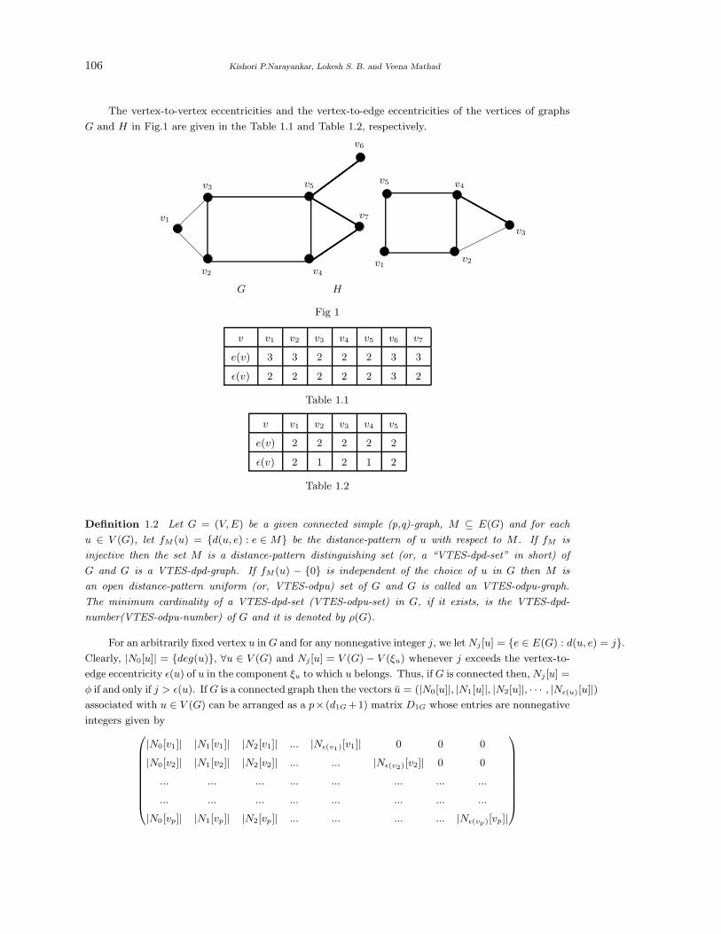
106 Kishori P.Narayankar, Lokesh S. B. and Veena Mathad
The vertex-to-vertex eccentricities and the vertex-to-edge eccentricities of the vertices of graphs
G and H in Fig.1 are given in the Table 1.1 and Table 1.2, respectively.
v3 v5
v6
v7
v4v2
v1
v5 v4
v2
v3
v1
G H
Fig 1
v v1 v2 v3 v4 v5 v6 v7
e(v) 3 3 2 2 2 3 3
ǫ(v) 2 2 2 2 2 3 2
Table 1.1
v v1 v2 v3 v4 v5
e(v) 2 2 2 2 2
ǫ(v) 2 1 2 1 2
Table 1.2
Definition 1.2 Let G = (V, E) be a given connected simple (p,q)-graph, M ⊆ E(G) and for each
u ∈ V (G), let fM (u) = {d(u, e) : e ∈ M} be the distance-pattern of u with respect to M . If fM is
injective then the set M is a distance-pattern distinguishing set (or, a “VTES-dpd-set” in short) of
G and G is a VTES-dpd-graph. If fM (u) − {0} is independent of the choice of u in G then M is
an open distance-pattern uniform (or, VTES-odpu) set of G and G is called an VTES-odpu-graph.
The minimum cardinality of a VTES-dpd-set (VTES-odpu-set) in G, if it exists, is the VTES-dpd-
number(VTES-odpu-number) of G and it is denoted by ρ(G).
For an arbitrarily fixed vertex u in G and for any nonnegative integer j, we let Nj [u] = {e ∈ E(G) : d(u, e) = j}.Clearly, |N0[u]| = {deg(u)}, ∀u ∈ V (G) and Nj [u] = V (G) − V (ξu) whenever j exceeds the vertex-to-
edge eccentricity ǫ(u) of u in the component ξu to which u belongs. Thus, if G is connected then, Nj [u] =
φ if and only if j > ǫ(u). If G is a connected graph then the vectors u = (|N0[u]|, |N1[u]|, |N2[u]|, · · · , |Nǫ(u)[u]|)associated with u ∈ V (G) can be arranged as a p× (d1G +1) matrix D1G whose entries are nonnegative
integers given by
|N0[v1]| |N1[v1]| |N2[v1]| ... |Nǫ(v1)[v1]| 0 0 0
|N0[v2]| |N1[v2]| |N2[v2]| ... ... |Nǫ(v2)[v2]| 0 0
... ... ... ... ... ... ... ...
... ... ... ... ... ... ... ...
|N0[vp]| |N1[vp]| |N2[vp]| ... ... ... ... |Nǫ(vp)[vp]|
Vertex-to-Edge-set Distance Neighborhood Pattern Matrices 107
where d1G denotes the vertex-toedge diameter of G; we call D1G VTES-distance neighborhood pattern
matrix (or, VTES-dnp-matrix) of G. For a VTES-dnp-matrix the following observations are immediate.
Observation 1.3 Entries in the first column of D1G are nonzero entries.
Observation 1.34 In each row of D1G, entry zero will be after some nonzero entries. Zero entries
may or may not be present in rows.
Observation 1.5 The entries in the first column of D1G correspond to the degrees of the corresponding
vertices in G.
Proposition 1.6 For each u ∈ V (G) of a connected graph G, {Nj [u] : Nj [u] 6= φ, 0 ≤ j ≤ d1G} gives
a partition of E(G).
Proof If possible, let e ∈ Nj [u] ∩ Nk[u], for some e ∈ E(G) and u ∈ V (G). Then d(u, e) = j
and d(u, e) = k, and hence j = k. Therefore,Nj [u] ∩ Nk[u] = φ for any (j, k) with j 6= k. Now,
clearly,⋃d1G
j=o Nj [u] ⊆ E(G). Also, for any e ∈ E(G), since G is connected, d(u, e) = k, for some k ∈{0, 1, 2, · · · , d1G}. That is, e ∈ Nk[u] for some k ∈ {0, 1, 2, · · · , d1G} which implies E(G) ⊆ ⋃d1G
j=o Nj [u].
Hence⋃d1G
j=o Nj [u] = E(G). 2Corollary 1.7 Each row of the VTES-dnp-matrix D1G of a graph G is the partition of |E(G)|. Hence,
sum of the entries in each row of the VTES-dnp-matrix D1G of a graph G is equal to the number of
edges of G.
§2. M-VTES-Distance Neighborhood Pattern Matrix of a Graph
Given an arbitrary nonempty subset M ⊆ E(G) of G and for each u ∈ V (G), define NMj [u] =
{e ∈ M : d(u, e) = j}; clearly then NE(G)j [u] = Nj [u]. One can define the M -VTES-eccentricity of
u as the largest integer for which NMj [u] 6= φ and the p × (d1G + 1) nonnegative integer matrix
DM1G = (|NM
j [u]|) is called the M -VTES-distance neighborhood pattern (or, M -VTES-dnp) matrix of
G. D∗MG is obtained from DM
1G by replacing each nonzero entry by 1.
B.D.Acarya ([1]) defined VTES-dnp matrix of any graph and in particular, M -VTES-dnp matrix
of VTES-dpd-graph as follows:
Definition 2.1 Let G = (V, E) be a given connected simple (p,q)-graph, M( 6= φ) ⊆ E(G) and u ∈ V (G).
Then, the M-VTES-distance-pattern of u is the set fM (u) = {d(u, e) : e ∈ M}. Clearly, fM (u) ={
j : NMj [u] 6= φ
}
. Hence, in particular, if fM : u 7−→ fM (u) is an injective function, then the set M is
a VTES-distance-pattern distinguishing set ( or, a “VTES-dpd-set” is short) of G and if fM (u)−{0} is
independent of the choice of u in G then M is a VTES-open distance-pattern uniform (or, VTES-odpu)
set of G. A graph G with a VTES-dpd-set(VTES-odpu-set) is called a VTES-dpd-(VTES-odpu)-graph.
Following are some interesting results on M -VTES-dnp matrix of a connected nontrivial graph G.
Observation 2.2 Both DM1G and D∗M
1G do not admit null rows.
108 Kishori P.Narayankar, Lokesh S. B. and Veena Mathad
Proposition 2.3 For each u ∈ V (G),
NM0 [u] =
M ∩ Du, if M ∩ Du 6= φ;
∅, if M ∩ Du = φ,
where Du = {ei : 1 ≤ i ≤ degu and u is adjacent to ei }.Therefore, the entries in the first column of DM
1G are zero or an integer k, 1 ≤ k ≤ degu and the
entries in the first column of D∗M1G are either 0 or 1.
Remark 2.4 It should be noted that Observation is not true in the case of D∗M1G .
Remark 2.5 For a graph G ∼= Cn,
vertex-toedge diameter d1G=
n−22
if n is even integer
n−12
if n is odd integer
Remark 2.6 For a graph G ∼= Pn, n ≥ 2, the vertex-to-edge diameter d1G= n − 2.
Lemma 2.7 is similar to Proposition 1.6.
Lemma 2.7 For each u ∈ V (G) of a connected graph G,{
NMj [u] : NM
j [u] 6= ∅, 0 ≤ j ≤d1G} gives a partition of M .
Proof If possible, let e ∈ NMj [u] ∩ NM
k [u], for some e ∈ M and u ∈ V (G). Then d(u, e) = j
and d(u, e) = k, and hence j = k. Therefore, NMj [u] ∩ NM
k [u] = φ for any (j, k) with j 6= k. Now,
clearly,⋃d1G
j=o NMj [u] ⊆ M . Also, for any e ∈ M , since G is connected, d(u, e) = k, for some k ∈
{0, 1, 2, · · · , d1G}. That is, e ∈ NMk [u] for some k ∈ {0, 1, 2, · · · , d1G} which implies M ⊆ ⋃d1G
j=o NMj [u].
Hence⋃d1G
j=o NMj [u] = M . 2
Corollary 2.8 Each row of DM1G is a partition of |M |.
Corollary 2.9 Sum of the entries in each row of DM1G gives |M | and sum of the entries in each row of
D∗M1G is less than or equal to |M |.
§3. M-VTES-Distance Neighborhood Pattern Matrix of a VTES-dpd Graph
In this section we find out some results of D∗M1G of a VTES-dpd-graph. From the definition of D∗M
1G ,
we have the following observations.
Observation 3.1 In any graph G, a nonempty M ⊆ E(G) is a VTES-dpd-set if and only if no two
rows of D∗M1G are identical.
The following Theorem 3.2 shows that M is a proper subset of E(G).
Theorem 3.2 For a VTES-dpd-graph G of order p and size q, a VTES-dpd set M is such that
3 ≦ |M | ≦ q − 1.
Proof For lower bound, let M be a VTES-dpd set. If M = {e}, for some e = uv ∈ E(G), then
D∗M1G contains a 2× (d1G + 1) submatrix, such that the rows of submatrix represent the M -VTES-dnp
of the vertices u and v in D∗M1G . That is, entry 1 is at the first column of submatrix and the rows are
as shown below,
Vertex-to-Edge-set Distance Neighborhood Pattern Matrices 109
1 0 0 · · · 0
1 0 0 · · · 0
.
Hence D∗M1G contains identical rows, Therefore M is not a VTES-dpd-set and hence |M | 6= 1.
Next, suppose M = {ek, el} for some ek = uiuj ∈ E(G) and el = vivj ∈ E(G). We consider the
following cases.
Case 1. ek is adjacent to el. Let uj = vi. Then d1(ui, ek) = d(vj , el) = 0 and d(ui, el) =
d(vj , ek) = 1. Then D∗M1G contains a 2× (d1G +1) submatrix, such that the rows of submatrix represent
the M -VTES-dnp of the vertices ui and vj in D∗M1G . That is, entry 1 is at the first and second column
of submatrix and rows are as shown below.
1 1 0 0 · · · 0
1 1 0 0 · · · 0
.
Case 2. ek is not adjacent to el. Then the rows of the 2× (d1G + 1) submatrix corresponding to
the M-VTES-dnp of ui and vj in D∗M1G are as follows.
1 0 0 · · · 1 0 0 · · · 0
1 0 0 · · · 1 0 0 · · · 0
Thus D∗M1G contains identical rows if |M | = 2 and so, M is not a VTES-dpd-set. Hence the lower bound
follows.
For upper bound, suppose on contrary, there exist a VTES-dpd-set M with |M | = q. We prove
by induction on p ≥ 2.
Suppose p = 2 with |M | = q. Then the graph G ∼= K2 and |M | = 1. By lower bound |M | ≥ 3, a
contradiction. Suppose p = 3 with |M | = q then the graph G is either K1,2 or K3. If G ∼= K1,2, with
|M | = q = 2. By lower bound |M | ≥ 3, a contradiction. If G ∼= K3 with |M | = q = 3. Then, we have
a VTES-dpd-matrix
D∗M1G =
1 1
1 1
1 1
.
Clearly rows are identical hence, a contradiction. Therefore |M | 6= q for p = 2 and p = 3. Suppose that
|M | 6= q for p = n. We claim that |M | 6= q for p = n + 1. Let V (G) = {v1, v2, · · · , vn, vn+1} be the
vertex set of G. One can observe that every graph has atleast one vertex-to-edge central vertex. Let
C1(G) be set of vertex-to-edge central vertices. We consider the following cases.
Case 1. |C1(G)| = 1. Let vi ∈ C1(G), then D∗M1G contains a (degvi)× (d1G + 1) submatrix, rows
of which represent the M -VTES-dnp of the vertices vj ∈ N(vi); j = 1, 2, · · · , degvi in D∗M1G as shown
below.
1 1 1 0 · · · 0
· · · · · · · · · · · · · · · · · ·1 1 1 0 · · · 0
· · · · · · · · · · · · · · · · · ·1 1 1 0 · · · 0
.
110 Kishori P.Narayankar, Lokesh S. B. and Veena Mathad
Hence D∗M1G contains identical rows , a contradiction. Hence |M | 6= q for p = n + 1. By mathematical
induction, the result follows for all p.
Case 2. |C1(G)| ≥ 2. Let C1(G) = {v1, v2, · · · , vi}, i ≥ 2. For every vi,vj ∈ C1(G), there exists
an edge ek such that d(vi, ek) =d(vj , ek). Then D∗M1G contains a 2 × (d1G + 1) submatrix, the rows of
which represent the M -VTES-dnp of vertices vi and vj in D∗M1G as shown below.
1 1 1 0 · · · 0
1 1 1 0 · · · 0
.
Hence D∗M1G contains identical rows, a contradiction. Thus, |M | ≦ q − 1. 2
Lemma 3.3 If d1G ≤ 2, then G does not possess a VTES-dpd-set.
Proof One can verify from [6] Appendix 1,Table A1. 2Corollary 3.4 If G ∼= Kn, Kn − e or Km,n, then G does not possess a VTES-dpd-set.
Theorem 3.5 A graph G ∼= Pn of order n admits a VTES-dpd-set if and only if n ≥ 5.
Proof Suppose that G ∼= Pn, where Pn = (v1, e1, v2, e2, v3, e3, · · · , en−1, vn, ). Let M = {e1, e2, e4}.Then
D∗M1G =
1 1 0 1 0 0 · · · 0 0 0 0 0 0
1 0 1 0 0 0 · · · 0 0 0 0 0 0
1 1 0 0 0 0 · · · 0 0 0 0 0 0
1 1 1 0 0 0 · · · 0 0 0 0 0 0
1 0 1 1 0 0 · · · 0 0 0 0 0 0
0 1 0 1 1 0 · · · 0 0 0 0 0 0
0 0 1 0 1 1 · · · 0 0 0 0 0 0
· · · · · · · · · · · · · · · · · · · · · · · · · · · · · · · · · · · · · · ·0 0 0 0 0 0 · · · 1 0 1 1 0 0
0 0 0 0 0 0 · · · 0 1 0 1 1 0
0 0 0 0 0 0 · · · 0 0 1 0 1 1
.
Now, we can partition D∗M1G into two submatrices say, A and B where A is a 4×(d1G+1) submatrix
of the form
1 1 0 1 0 0 · · · 0 0 0 0 0 0
1 0 1 0 0 0 · · · 0 0 0 0 0 0
1 1 0 0 0 0 · · · 0 0 0 0 0 0
1 1 1 0 0 0 · · · 0 0 0 0 0 0
.
Again we can find the 4 × 4 submatrix A1 of A which is of the form
1 1 0 1
1 0 1 0
1 1 0 0
1 1 1 0
.
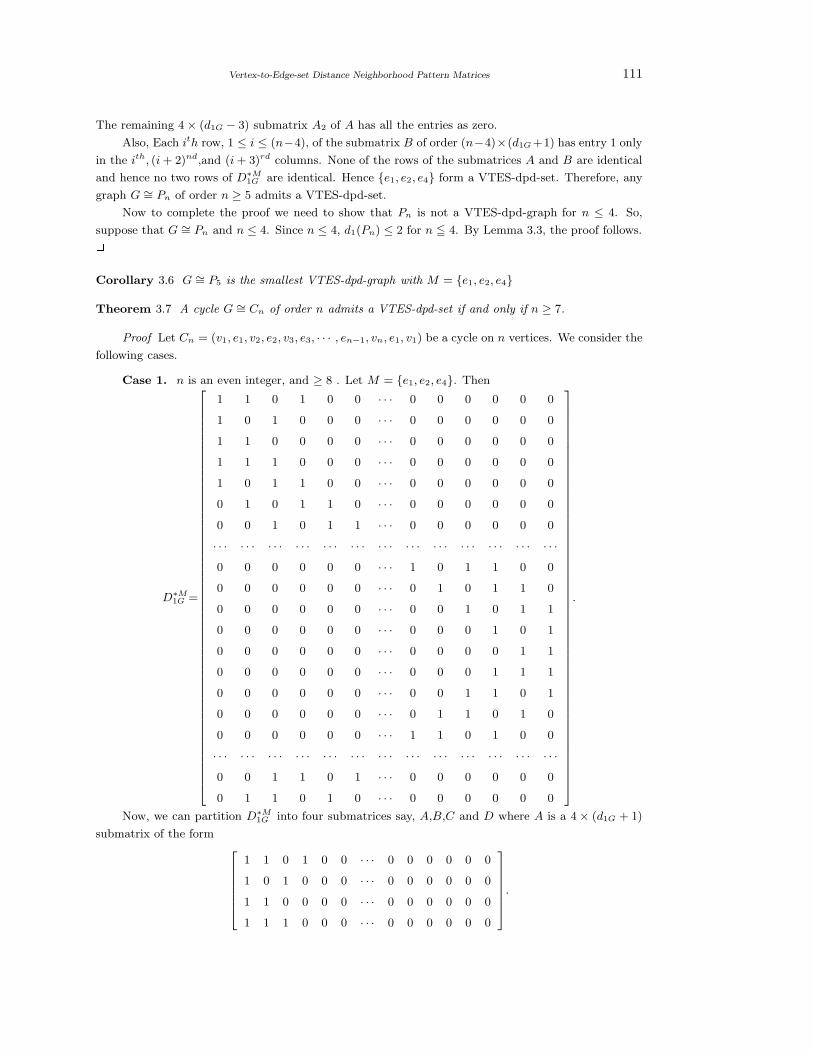
Vertex-to-Edge-set Distance Neighborhood Pattern Matrices 111
The remaining 4 × (d1G − 3) submatrix A2 of A has all the entries as zero.
Also, Each ith row, 1 ≤ i ≤ (n−4), of the submatrix B of order (n−4)×(d1G +1) has entry 1 only
in the ith, (i + 2)nd,and (i + 3)rd columns. None of the rows of the submatrices A and B are identical
and hence no two rows of D∗M1G are identical. Hence {e1, e2, e4} form a VTES-dpd-set. Therefore, any
graph G ∼= Pn of order n ≥ 5 admits a VTES-dpd-set.
Now to complete the proof we need to show that Pn is not a VTES-dpd-graph for n ≤ 4. So,
suppose that G ∼= Pn and n ≤ 4. Since n ≤ 4, d1(Pn) ≤ 2 for n ≦ 4. By Lemma 3.3, the proof follows.2Corollary 3.6 G ∼= P5 is the smallest VTES-dpd-graph with M = {e1, e2, e4}
Theorem 3.7 A cycle G ∼= Cn of order n admits a VTES-dpd-set if and only if n ≥ 7.
Proof Let Cn = (v1, e1, v2, e2, v3, e3, · · · , en−1, vn, e1, v1) be a cycle on n vertices. We consider the
following cases.
Case 1. n is an even integer, and ≥ 8 . Let M = {e1, e2, e4}. Then
D∗M1G =
1 1 0 1 0 0 · · · 0 0 0 0 0 0
1 0 1 0 0 0 · · · 0 0 0 0 0 0
1 1 0 0 0 0 · · · 0 0 0 0 0 0
1 1 1 0 0 0 · · · 0 0 0 0 0 0
1 0 1 1 0 0 · · · 0 0 0 0 0 0
0 1 0 1 1 0 · · · 0 0 0 0 0 0
0 0 1 0 1 1 · · · 0 0 0 0 0 0
· · · · · · · · · · · · · · · · · · · · · · · · · · · · · · · · · · · · · · ·0 0 0 0 0 0 · · · 1 0 1 1 0 0
0 0 0 0 0 0 · · · 0 1 0 1 1 0
0 0 0 0 0 0 · · · 0 0 1 0 1 1
0 0 0 0 0 0 · · · 0 0 0 1 0 1
0 0 0 0 0 0 · · · 0 0 0 0 1 1
0 0 0 0 0 0 · · · 0 0 0 1 1 1
0 0 0 0 0 0 · · · 0 0 1 1 0 1
0 0 0 0 0 0 · · · 0 1 1 0 1 0
0 0 0 0 0 0 · · · 1 1 0 1 0 0
· · · · · · · · · · · · · · · · · · · · · · · · · · · · · · · · · · · · · · ·0 0 1 1 0 1 · · · 0 0 0 0 0 0
0 1 1 0 1 0 · · · 0 0 0 0 0 0
.
Now, we can partition D∗M1G into four submatrices say, A,B,C and D where A is a 4 × (d1G + 1)
submatrix of the form
1 1 0 1 0 0 · · · 0 0 0 0 0 0
1 0 1 0 0 0 · · · 0 0 0 0 0 0
1 1 0 0 0 0 · · · 0 0 0 0 0 0
1 1 1 0 0 0 · · · 0 0 0 0 0 0
.
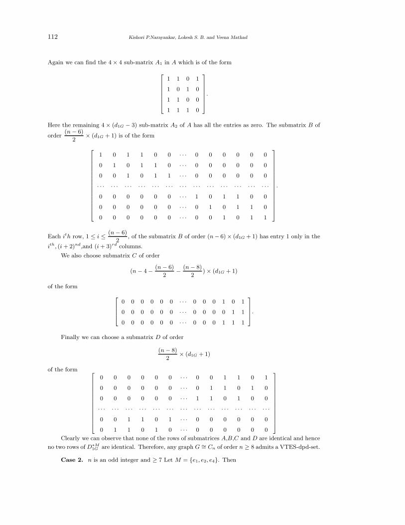
112 Kishori P.Narayankar, Lokesh S. B. and Veena Mathad
Again we can find the 4 × 4 sub-matrix A1 in A which is of the form
1 1 0 1
1 0 1 0
1 1 0 0
1 1 1 0
.
Here the remaining 4 × (d1G − 3) sub-matrix A2 of A has all the entries as zero. The submatrix B of
order(n − 6)
2× (d1G + 1) is of the form
1 0 1 1 0 0 · · · 0 0 0 0 0 0
0 1 0 1 1 0 · · · 0 0 0 0 0 0
0 0 1 0 1 1 · · · 0 0 0 0 0 0
· · · · · · · · · · · · · · · · · · · · · · · · · · · · · · · · · · · · · · ·0 0 0 0 0 0 · · · 1 0 1 1 0 0
0 0 0 0 0 0 · · · 0 1 0 1 1 0
0 0 0 0 0 0 · · · 0 0 1 0 1 1
.
Each ith row, 1 ≤ i ≤ (n − 6)
2, of the submatrix B of order (n− 6)× (d1G + 1) has entry 1 only in the
ith, (i + 2)nd,and (i + 3)rd columns.
We also choose submatrix C of order
(n − 4 − (n − 6)
2− (n − 8)
2) × (d1G + 1)
of the form
0 0 0 0 0 0 · · · 0 0 0 1 0 1
0 0 0 0 0 0 · · · 0 0 0 0 1 1
0 0 0 0 0 0 · · · 0 0 0 1 1 1
.
Finally we can choose a submatrix D of order
(n − 8)
2× (d1G + 1)
of the form
0 0 0 0 0 0 · · · 0 0 1 1 0 1
0 0 0 0 0 0 · · · 0 1 1 0 1 0
0 0 0 0 0 0 · · · 1 1 0 1 0 0
· · · · · · · · · · · · · · · · · · · · · · · · · · · · · · · · · · · · · · ·0 0 1 1 0 1 · · · 0 0 0 0 0 0
0 1 1 0 1 0 · · · 0 0 0 0 0 0
Clearly we can observe that none of the rows of submatrices A,B,C and D are identical and hence
no two rows of D∗M1G are identical. Therefore, any graph G ∼= Cn of order n ≥ 8 admits a VTES-dpd-set.
Case 2. n is an odd integer and ≥ 7 Let M = {e1, e2, e4}. Then
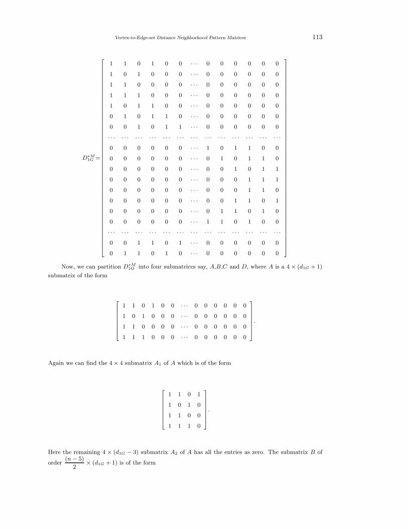
Vertex-to-Edge-set Distance Neighborhood Pattern Matrices 113
D∗M1G =
1 1 0 1 0 0 · · · 0 0 0 0 0 0
1 0 1 0 0 0 · · · 0 0 0 0 0 0
1 1 0 0 0 0 · · · 0 0 0 0 0 0
1 1 1 0 0 0 · · · 0 0 0 0 0 0
1 0 1 1 0 0 · · · 0 0 0 0 0 0
0 1 0 1 1 0 · · · 0 0 0 0 0 0
0 0 1 0 1 1 · · · 0 0 0 0 0 0
· · · · · · · · · · · · · · · · · · · · · · · · · · · · · · · · · · · · · · ·0 0 0 0 0 0 · · · 1 0 1 1 0 0
0 0 0 0 0 0 · · · 0 1 0 1 1 0
0 0 0 0 0 0 · · · 0 0 1 0 1 1
0 0 0 0 0 0 · · · 0 0 0 1 1 1
0 0 0 0 0 0 · · · 0 0 0 1 1 0
0 0 0 0 0 0 · · · 0 0 1 1 0 1
0 0 0 0 0 0 · · · 0 1 1 0 1 0
0 0 0 0 0 0 · · · 1 1 0 1 0 0
· · · · · · · · · · · · · · · · · · · · · · · · · · · · · · · · · · · · · · ·0 0 1 1 0 1 · · · 0 0 0 0 0 0
0 1 1 0 1 0 · · · 0 0 0 0 0 0
Now, we can partition D∗M1G into four submatrices say, A,B,C and D, where A is a 4 × (d1G + 1)
submatrix of the form
1 1 0 1 0 0 · · · 0 0 0 0 0 0
1 0 1 0 0 0 · · · 0 0 0 0 0 0
1 1 0 0 0 0 · · · 0 0 0 0 0 0
1 1 1 0 0 0 · · · 0 0 0 0 0 0
.
Again we can find the 4 × 4 submatrix A1 of A which is of the form
1 1 0 1
1 0 1 0
1 1 0 0
1 1 1 0
.
Here the remaining 4 × (d1G − 3) submatrix A2 of A has all the entries as zero. The submatrix B of
order(n − 5)
2× (d1G + 1) is of the form
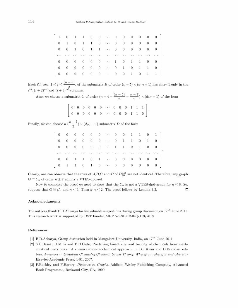
114 Kishori P.Narayankar, Lokesh S. B. and Veena Mathad
1 0 1 1 0 0 · · · 0 0 0 0 0 0
0 1 0 1 1 0 · · · 0 0 0 0 0 0
0 0 1 0 1 1 · · · 0 0 0 0 0 0
· · · · · · · · · · · · · · · · · · · · · · · · · · · · · · · · · · · · · · ·0 0 0 0 0 0 · · · 1 0 1 1 0 0
0 0 0 0 0 0 · · · 0 1 0 1 1 0
0 0 0 0 0 0 · · · 0 0 1 0 1 1
.
Each ith row, 1 ≤ i ≤ (n − 5)
2, of the submatrix B of order (n− 5)× (d1G + 1) has entry 1 only in the
ith, (i + 2)nd,and (i + 3)rd columns.
Also, we choose a submatrix C of order (n − 4 − (n − 5)
2− n − 7
2) × (d1G + 1) of the form
0 0 0 0 0 0 · · · 0 0 0 1 1 1
0 0 0 0 0 0 · · · 0 0 0 1 1 0
.
Finally, we can choose a (n − 7
2) × (d1G + 1) submatrix D of the form
0 0 0 0 0 0 · · · 0 0 1 1 0 1
0 0 0 0 0 0 · · · 0 1 1 0 1 0
0 0 0 0 0 0 · · · 1 1 0 1 0 0
· · · · · · · · · · · · · · · · · · · · · · · · · · · · · · · · · · · · · · ·0 0 1 1 0 1 · · · 0 0 0 0 0 0
0 1 1 0 1 0 · · · 0 0 0 0 0 0
.
Clearly, one can observe that the rows of A,B,C and D of D∗M1G are not identical. Therefore, any graph
G ∼= Cn of order n ≥ 7 admits a VTES-dpd-set.
Now to complete the proof we need to show that the Cn is not a VTES-dpd-graph for n ≤ 6. So,
suppose that G ∼= Cn and n ≤ 6. Then d1G ≤ 2. The proof follows by Lemma 3.3. 2Acknowledgments
The authors thank B.D.Acharya for his valuable suggestions during group discussion on 17th June 2011.
This research work is supported by DST Funded MRP.No–SB/EMEQ-119/2013.
References
[1] B.D.Acharya, Group discussion held in Mangalore University, India, on 17th June 2011.
[2] S.C.Basak, D.Mills and B.D.Gute, Predicting bioactivity and toxicity of chemicals from math-
ematical descriptors: A chemical-cum-biochemical approach, In D.J.Klein and D.Brandas, edi-
tors, Advances in Quantum Chemistry:Chemical Graph Theory: Wherefrom,wherefor and whereto?
Elsevier-Academic Press, 1-91, 2007.
[3] F.Buckley and F.Harary, Distance in Graphs, Addison Wesley Publishing Company, Advanced
Book Programme, Redwood City, CA, 1990.
Vertex-to-Edge-set Distance Neighborhood Pattern Matrices 115
[4] K.A.Germina, Alphy Joseph and Sona Jose, Distance neighborhood pattern matrices, Eur. J.
Pure Appl. Math., Vol.3, No.4, 2010, 748-764.
[5] F.Harary and Melter, On the metric dimension of a graph, Ars Combin., 2,191-195, 1976.
[6] F.Harary, Graph Theory, Addison Wesley Publ. Comp., Reading, Massachusetts, 1969.
[7] Kishori P.Narayankar, Lokesh S.B. Edge-Distance Pattern Distingushing Graph, Submitted.
[8] D.H.Rouvrey, Predicting chemistry from topology, Scientific American, 254, 9, 40-47,1986.
[9] A.P.Santhakumaran, Center of a graph with respect to edge, SCIENTIA Series A: Mathematical
Sciences, Vol. 19 (2010), 13-23.
International J.Math. Combin. Vol.3(2015), 116-124
Extended Results on Complementary Tree Domination
Number and Chromatic Number of Graphs
S.Muthammai
(Government Arts College for Women (Autonomous), Pudukkottai - 622 001, India)
P.Vidhya
(S.D.N.B.Vaishnav College for Women (Autonomous), Chennai - 600 044, India)
E-mail: [email protected], vidhya [email protected]
Abstract: For any graph G = (V, E) a subset D ⊆ V is a dominating set if every vertex in
V −D is adjacent to at least one vertex in D. A dominating set is said to be a complementary
tree dominating set if the induced subgraph < V −D > is a tree. The minimum cardinality
of a complementary tree dominating set is called the complementary tree domination number
and is denoted by γctd(G). In this paper, we find an upper bound for γctd(G)+χ(G) = 2p−5
and γctd(G) + χ(G) = 2p − 6, p is the number of vertices in G.
Key Words: Domination number, complementary tree domination.
AMS(2010): 05C69.
§1. Introduction
By a graph G = (V, E) we mean a finite undirected graph without loops or multiple edges. The order
and size of G are denoted by p and q respectively. For graph theoretical terms, we refer Harary [1] and
for terms related to domination we refer Haynes et al. [2].
A subset D of V is said to be a dominating set in G if every vertex in V − D is adjacent to at
least one vertex in D. The domination number γ(G) is the minimum cardinality of a dominating set in
G. The concept of complementary tree domination was introduced by Muthammai, Bhanumathi and
Vidhya [3]. A dominating set D is called a complementary tree domination set if the induced subgraph
< V − D > is a tree. The minimum cardinality of a complementary tree dominating set is called the
complementary tree domination number of G, denoted by γctd(G) and such a set D is called a γctd set.
The minimum number of colours required to colour all the vertices such that adjacent vertices do not
receive the same colour is the chromatic number χ(G).
In this paper, we obtain sharp upper bound for γctd(G)+χ(G) = 2p−5 and γctd(G)+χ(G) = 2p−6.
We use the following previous results.
Theorem 1.1([1]) For any connected graph G, χ(G) ≤ ∆(G) + 1.
Theorem 1.2([3]) For any connected graph G with p ≥ 2, γctd(G) ≤ p − 1.
1Received December 29, 2014, Accepted August 30, 2015.
Extended Results on Complementary Tree Domination Number and Chromatic Number of Graphs 117
Theorem 1.3([3]) Let G be a connected graph with p ≥ 2. γctd(G) = p − 1 if and only if G is a star
on p vertices.
Theorem 1.4([3]) Let G be a connected graph containing a cycle. Then γctd(G) = p − 2 if and only
if G is isormorphic to one of the following graphs. Cp, Kp or G is the graph obtained by attaching
pendant edges at at least one of the vertices of a complete graph.
Theorem 1.5([3]) Let T be a tree with p vertices which is not a star. Then γctd(T ) = p − 2 if and
only if T is a path or T is obtained by attaching pendant edges at at least one of the end vertices.
Theorem 1.6([4]) For any connected graph G, γctd(G) + χ(G) ≤ 2p − 1, (p ≥ 2). The equality holds
if and only if G ∼= K2.
Theorem 1.7([4]) For any connected graph G, γctd(G) + χ(G) = 2p− 2 (p ≥ 3) if and only if G ∼= P3
or Kp, p ≥ 4.
Theorem 1.8([4]) For any connected graph G, γctd(G) + χ(G) = 2p − 3 (p ≥ 4) if and only if G is
a star on four vertices or G is the graph obtained by adding a pendant edge at exactly one vertex of
Kp−1.
Theorem 1.9([4]) For any connected graph G, on p vertices, γctd(G) + χ(G) = 2p − 4 (p ≥ 5) if and
only if G is one of the following graphs.
(1) G is a star on 5 vertices;
(2) G is a cycle on 4 (or) 5 vertices;
(3) G is the graph obtained by attaching exactly two pendant edges at one vertex or two vertices
of Kp−2;
(4) is the graph obtained by joining a new vertex to j (2 ≤ j ≤ p − 2) vertices of Kp−1.
§2. Main Results
Notation 2.1 The following notations are used in this paper:
(1) Kn(p − n) is the set of graphs on n vertices obtained from Kn by attaching (p − n), (p > n)
pendant edges at the vertices of Kn.
(2) Kn(Pm) is the graph obtained from Kn by attaching a pendant edge of Pm to any one vertex
of Kn.
(3) K′n(H) is the set of graphs obtained from Kn by joining each of the vertices of the graph H
to the same i (1 ≤ i ≤ n − 1) vertices of Kn.
(4) K′′n(H) is the set of graphs obtained from Kn by joining each of the vertices of the graph H
to distinct (n − 1) vertices of Kn.
(5) K′′′n (H) is the set of graphs obtained from Kn by joining all the vertices of H , each is adjacent
to at least i (2 ≤ i ≤ n − 1) vertices of Kn.
(6) F1(Kn, 2K1) is the set of graphs obtained from Kn by joining one vertex of 2K1 to i (2 ≤ i ≤n − 1) vertices of Kn and the other vertex to any one vertex of Kn.
(7) F21(Kn, K2) is the set of graphs obtained from Kn by joining one vertex of K2 to i (1 ≤ i ≤n − 1) vertices of Kn.
(8) F22(Kn, K2) is the set of graphs obtained from Kn by joining each of the vertices of K2 to i
(1 ≤ i ≤ n − 1) distinct vertices of Kn.
118 S.Muthammai and P.Vidhya
(9) F3(Kn, 3K1) is the set of graphs obtained from Kn by joining one vertex of 3K1 to any of the
i (1 ≤ i ≤ n − 1) vertices of Kn and each of other two vertices of 3K1 to exactly one vertex of Kn.
(10) F41(Kn, K2 ∪K1) is the set of graphs obtained from Kn by joining one vertex of K2 and the
vertex of K1 to distinct (n − 1) vertices of Kn.
(11) F42(Kn, K2 ∪ K1) is the set of graphs obtained from Kn by joining one vertex of K2 to i
(1 ≤ i ≤ n − 1) vertices of Kn and the vertex of K1 to any one vertex of Kn.
(12) F43(Kn, K2 ∪ K1) is the set of graphs obtained from Kn by joining each of the vertices of
K2 ∪ K1 to vertices of Kn such that each vertex of K2 ∪ K1 is adjacent to exactly one vertex of Kn.
(13) F51(Kn, P3) is the set of graphs obtained from Kn by joining the central vertex of P3 to i
(1 ≤ i ≤ n − 1) vertices of Kn.
(14) F52(Kn, P3) is the set of graphs obtained from Kn by joining a pendant vertex and the central
vertex of P3 to the same i (1 ≤ i ≤ n − 1) vertices of Kn.
(15) F53(Kn, P3) is the set of graphs obtained from Kn by joining a pendant vertex and the central
vertex of P3 to distinct (n − 1) vertices of Kn.
In the following γctd(G) + χ(G) = 2p − 5 and γctd(G) + χ(G) = 2p − 6 are found.
Theorem 2.1 Let G be a connected graph with p (p ≥ 6) vertices then γctd(G) + χ(G) = 2p− 5 if and
only if G is one of the following graphs:
(a) G is a star (or) a cycle on 6 vertices;
(b) G ∈ Kp−3(3);
(c) G ∈ K′p−2(K2);
(d) G ∈ F1(Kp−2, 2K1);
(e) G ∈ F21(Kp−2, K2).
Proof If G is one of the graphs given in the theorem, then γctd(G) + χ(G) = 2p − 5. Conversely,
assume γctd(G) + χ(G) = 2p − 5. This is possible only if
(i) γctd(G) = p − 1 and χ(G) = p − 4;
(ii) γctd(G) = p − 2 and χ(G) = p − 3;
(iii) γctd(G) = p − 3 and χ(G) = p − 2;
(iv) γctd(G) = p − 4 and χ(G) = p − 1;
(v) γctd(G) = p − 5 and χ(G) = p.
Case 1. γctd(G) = p − 1 and χ(G) = p − 4.
But, γctd(G) = p− 1 if and only if G is star K1,p−1 on p vertices (Theorem 1.3, [3]). For a star G,
χ(G) = 2. Therefore, χ(G) = p − 4 implies that p = 6 that is, G is a star on 6 vertices.
Case 2. γctd(G) = p − 2 and χ(G) = p − 3.
But, γctd(G) = p − 2 implies that G is one of the following graphs (a) Cp, cycle on p vertices
(b) Kp, complete graph on p vertices (c) G is the graph obtained by attaching pendant edges at least
one of the vertices of a complete graph (d) G is a path (e) G is obtained from a path of at least three
vertices, by attaching pendant edges at at least one of the end vertices of the path.
G cannot be one of the graphs mentioned in (b), (d) and (e), since if G ∼= Kp, then χ(G) = p and
if G is a path (or) as in (e), then χ(G) = 2 and hence p = 5.
If G ∼= Cp then χ(G) = p − 3 implies p = 5 (or) 6. But, G has at least 6 vertices and hence
G ∼= C6. Let G be a graph obtained by attaching pendant edge at at least one of the vertices of a
complete graph.
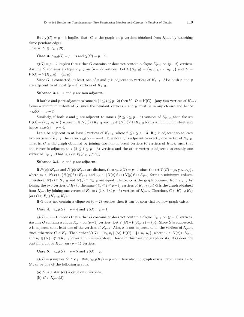
Extended Results on Complementary Tree Domination Number and Chromatic Number of Graphs 119
But χ(G) = p − 3 implies that, G is the graph on p vertices obtained from Kp−3 by attaching
three pendant edges.
That is, G ∈ Kp−3(3).
Case 3. γctd(G) = p − 3 and χ(G) = p − 2.
χ(G) = p− 2 implies that either G contains or does not contain a clique Kp−2 on (p− 2) vertices.
Assume G contains a clique Kp−2 on (p − 2) vertices. Let V (Kp−2) = {u1, u2, · · · , up−2} and D =
V (G) − V (Kp−2) = {x, y}.Since G is connected, at least one of x and y is adjacent to vertices of Kp−2. Also both x and y
are adjacent to at most (p − 3) vertices of Kp−2.
Subcase 3.1. x and y are non adjacent.
If both x and y are adjacent to same ui (1 ≤ i ≤ p−2) then V −D = V (G)−{any two vertices of Kp−2}forms a minimum ctd-set of G, since the pendant vertices x and y must be in any ctd-set and hence
γctd(G) = p − 2.
Similarly, if both x and y are adjacent to same i (2 ≤ i ≤ p − 3) vertices of Kp−2, then the set
V (G) − {x, y, ui, uj} where ui ∈ N(x) ∩ Kp−2 and uj ∈ (N(x))c ∩ Kp−2 forms a minimum ctd-set and
hence γctd(G) = p − 4.
Let x be adjacent to at least i vertices of Kp−2, where 2 ≤ i ≤ p − 3. If y is adjacent to at least
two vertices of Kp−2, then also γctd(G) = p−4. Therefore, y is adjacent to exactly one vertex of Kp−2.
That is, G is the graph obtained by joining two non-adjacent vertices to vertices of Kp−2, such that
one vertex is adjacent to i (2 ≤ i ≤ p − 3) vertices and the other vertex is adjacent to exactly one
vertex of Kp−2. That is, G ∈ F1(Kp−2, 2K1).
Subcase 3.2. x and y are adjacent.
If N(x)∩Kp−2 and N(y)∩Kp−2 are distinct, then γctd(G) = p−4, since the set V (G)−{x, y, ui, uj},where ui ∈ N(x) ∩ (N(y))c ∩ Kp−2 and uj ∈ (N(x))c ∩ (N(y))c ∩ Kp−2 forms a minimum ctd-set.
Therefore, N(x) ∩ Kp−2 and N(y) ∩ Kp−2 are equal. Hence, G is the graph obtained from Kp−2 by
joining the two vertices of K2 to the same i (1 ≤ i ≤ p−3) vertices of Kp−2 (or) G is the graph obtained
from Kp−2 by joining one vertex of K2 to i (1 ≤ i ≤ p− 3) vertices of Kp−2. Therefore, G ∈ K′p−2(K2)
(or) G ∈ F21(Kp−2, K2).
If G does not contain a clique on (p − 2) vertices then it can be seen that no new graph exists.
Case 4. γctd(G) = p − 4 and χ(G) = p − 1.
χ(G) = p− 1 implies that either G contains or does not contain a clique Kp−1 on (p− 1) vertices.
Assume G contains a clique Kp−1 on (p−1) vertices. Let V (G)−V (Kp−1) = {x}. Since G is connected,
x is adjacent to at least one of the vertices of Kp−1. Also, x is not adjacent to all the vertices of Kp−2,
since otherwise G ∼= Kp. Then either V (G)−{ui, uj} (or) V (G)−{x, ui, uj}, where ui ∈ N(x)∩Kp−1
and uj ∈ (N(x))c ∩Kp−1 forms a minimum ctd-set. Hence in this case, no graph exists. If G does not
contain a clique Kp−1 on (p − 1) vertices.
Case 5. γctd(G) = p − 5 and χ(G) = p.
χ(G) = p implies G ∼= Kp. But, γctd(Kp) = p − 2. Here also, no graph exists. From cases 1 - 5,
G can be one of the following graphs:
(a) G is a star (or) a cycle on 6 vertices;
(b) G ∈ Kp−3(3);
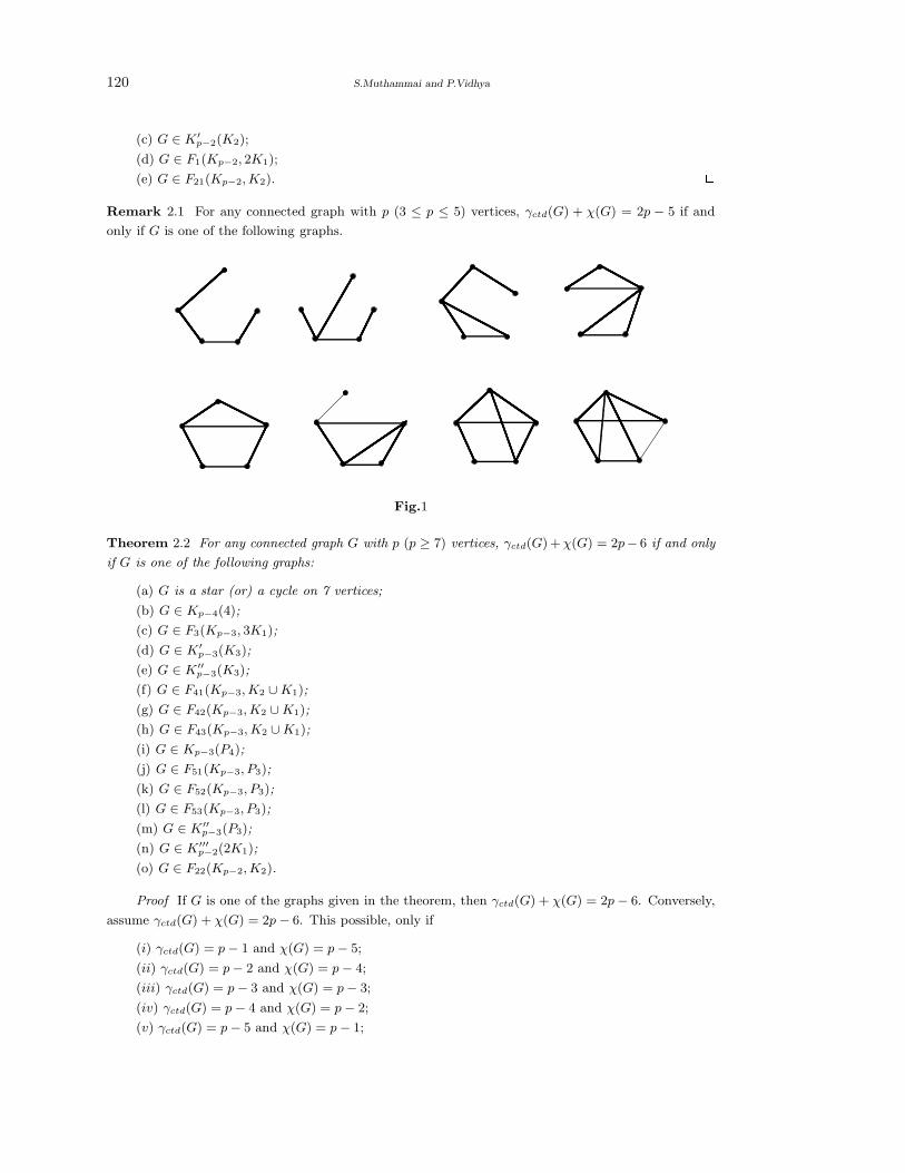
120 S.Muthammai and P.Vidhya
(c) G ∈ K′p−2(K2);
(d) G ∈ F1(Kp−2, 2K1);
(e) G ∈ F21(Kp−2, K2). 2Remark 2.1 For any connected graph with p (3 ≤ p ≤ 5) vertices, γctd(G) + χ(G) = 2p − 5 if and
only if G is one of the following graphs.
Fig.1
Theorem 2.2 For any connected graph G with p (p ≥ 7) vertices, γctd(G) + χ(G) = 2p− 6 if and only
if G is one of the following graphs:
(a) G is a star (or) a cycle on 7 vertices;
(b) G ∈ Kp−4(4);
(c) G ∈ F3(Kp−3, 3K1);
(d) G ∈ K′p−3(K3);
(e) G ∈ K′′p−3(K3);
(f) G ∈ F41(Kp−3, K2 ∪ K1);
(g) G ∈ F42(Kp−3, K2 ∪ K1);
(h) G ∈ F43(Kp−3, K2 ∪ K1);
(i) G ∈ Kp−3(P4);
(j) G ∈ F51(Kp−3, P3);
(k) G ∈ F52(Kp−3, P3);
(l) G ∈ F53(Kp−3, P3);
(m) G ∈ K′′p−3(P3);
(n) G ∈ K′′′p−2(2K1);
(o) G ∈ F22(Kp−2, K2).
Proof If G is one of the graphs given in the theorem, then γctd(G) + χ(G) = 2p − 6. Conversely,
assume γctd(G) + χ(G) = 2p − 6. This possible, only if
(i) γctd(G) = p − 1 and χ(G) = p − 5;
(ii) γctd(G) = p − 2 and χ(G) = p − 4;
(iii) γctd(G) = p − 3 and χ(G) = p − 3;
(iv) γctd(G) = p − 4 and χ(G) = p − 2;
(v) γctd(G) = p − 5 and χ(G) = p − 1;
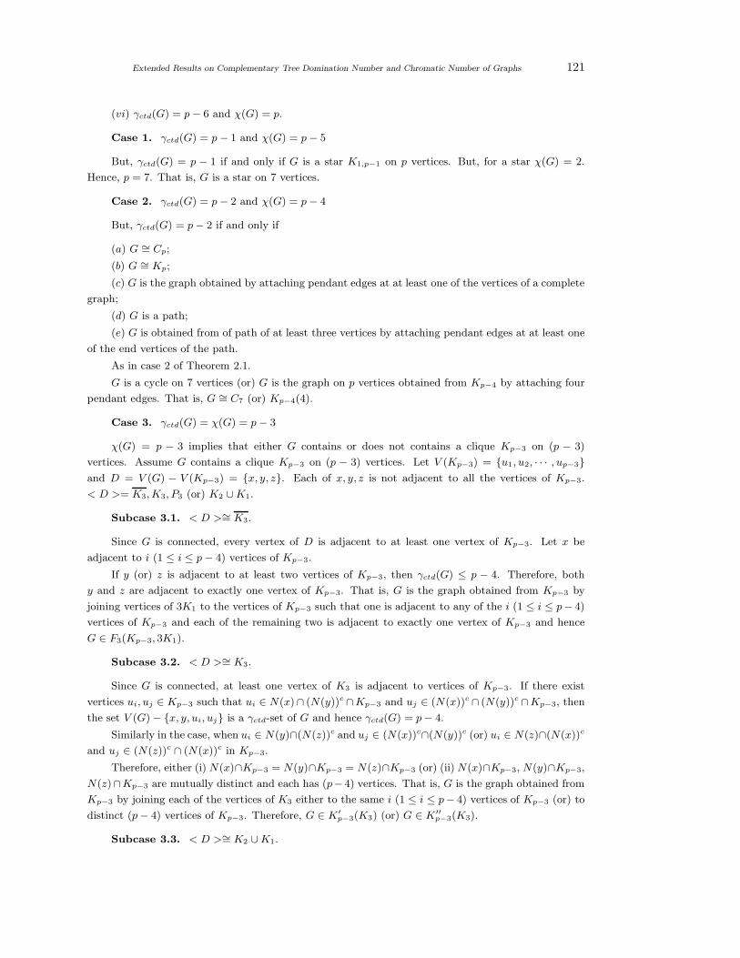
Extended Results on Complementary Tree Domination Number and Chromatic Number of Graphs 121
(vi) γctd(G) = p − 6 and χ(G) = p.
Case 1. γctd(G) = p − 1 and χ(G) = p − 5
But, γctd(G) = p − 1 if and only if G is a star K1,p−1 on p vertices. But, for a star χ(G) = 2.
Hence, p = 7. That is, G is a star on 7 vertices.
Case 2. γctd(G) = p − 2 and χ(G) = p − 4
But, γctd(G) = p − 2 if and only if
(a) G ∼= Cp;
(b) G ∼= Kp;
(c) G is the graph obtained by attaching pendant edges at at least one of the vertices of a complete
graph;
(d) G is a path;
(e) G is obtained from of path of at least three vertices by attaching pendant edges at at least one
of the end vertices of the path.
As in case 2 of Theorem 2.1.
G is a cycle on 7 vertices (or) G is the graph on p vertices obtained from Kp−4 by attaching four
pendant edges. That is, G ∼= C7 (or) Kp−4(4).
Case 3. γctd(G) = χ(G) = p − 3
χ(G) = p − 3 implies that either G contains or does not contains a clique Kp−3 on (p − 3)
vertices. Assume G contains a clique Kp−3 on (p − 3) vertices. Let V (Kp−3) = {u1, u2, · · · , up−3}and D = V (G) − V (Kp−3) = {x, y, z}. Each of x, y, z is not adjacent to all the vertices of Kp−3.
< D >= K3, K3, P3 (or) K2 ∪ K1.
Subcase 3.1. < D >∼= K3.
Since G is connected, every vertex of D is adjacent to at least one vertex of Kp−3. Let x be
adjacent to i (1 ≤ i ≤ p − 4) vertices of Kp−3.
If y (or) z is adjacent to at least two vertices of Kp−3, then γctd(G) ≤ p − 4. Therefore, both
y and z are adjacent to exactly one vertex of Kp−3. That is, G is the graph obtained from Kp−3 by
joining vertices of 3K1 to the vertices of Kp−3 such that one is adjacent to any of the i (1 ≤ i ≤ p− 4)
vertices of Kp−3 and each of the remaining two is adjacent to exactly one vertex of Kp−3 and hence
G ∈ F3(Kp−3, 3K1).
Subcase 3.2. < D >∼= K3.
Since G is connected, at least one vertex of K3 is adjacent to vertices of Kp−3. If there exist
vertices ui, uj ∈ Kp−3 such that ui ∈ N(x)∩ (N(y))c ∩Kp−3 and uj ∈ (N(x))c ∩ (N(y))c ∩Kp−3, then
the set V (G) − {x, y, ui, uj} is a γctd-set of G and hence γctd(G) = p − 4.
Similarly in the case, when ui ∈ N(y)∩(N(z))c and uj ∈ (N(x))c∩(N(y))c (or) ui ∈ N(z)∩(N(x))c
and uj ∈ (N(z))c ∩ (N(x))c in Kp−3.
Therefore, either (i) N(x)∩Kp−3 = N(y)∩Kp−3 = N(z)∩Kp−3 (or) (ii) N(x)∩Kp−3, N(y)∩Kp−3,
N(z)∩Kp−3 are mutually distinct and each has (p− 4) vertices. That is, G is the graph obtained from
Kp−3 by joining each of the vertices of K3 either to the same i (1 ≤ i ≤ p− 4) vertices of Kp−3 (or) to
distinct (p − 4) vertices of Kp−3. Therefore, G ∈ K′p−3(K3) (or) G ∈ K′′
p−3(K3).
Subcase 3.3. < D >∼= K2 ∪ K1.
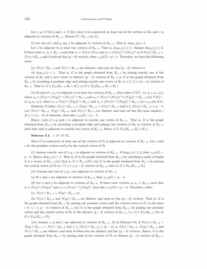
122 S.Muthammai and P.Vidhya
Let x, y ∈ V (K2) and z ∈ V (K1) since G is connected, at least one of the vertices of K2 and z is
adjacent to vertices of Kp−3. Denote G ∩ Kp−3 by G1.
(i) Let one of x and y, say x be adjacent to vertices of Kp−3. That is, degG1(y) = 1.
Let x be adjacent to at least two vertices of Kp−3. That is, degG1(x) ≥ 2. Assume degG1(z) ≥ 2.
If there exist ui, uj ∈ Kp−3 such that ui ∈ N(x)∩N(z) and uj ∈ (N(x))c∩(N(z))c or if N(x)∩Kp−3 =
N(z)∩Kp−3 and if each set has (p−4) vertices, then γctd(G) = p−4. Therefore, we have the following
cases:
(a) N(x) ∩ Kp−3 and N(z) ∩ Kp−3 are distinct, and each set has (p − 4) vertices or
(b) degG1(z) = 1. That is, G is the graph obtained from Kp−3 by joining exactly one of the
vertices of K2 and a new vertex to distinct (p − 4) vertices of Kp−3 or G is the graph obtained from
Kp−3 by attaching a pendant edge and joining exactly one vertex of K2 to i (1 ≤ i ≤ p− 4) vertices of
Kp−3. That is, G ∈ F41(Kp−3, K2 ∪ K1) or G ∈ F42(Kp−3, K2 ∪ K1).
(ii) If each of x, y, z is adjacent to at least two vertices of Kp−3, then either V (G)−{x, y, z, ui, uj},where ui ∈ N(x) ∩ (N(y))c ∩ (N(z))c ∩ Kp−3 and uj ∈ N(z) ∩ (N(x))c ∩ (N(y))c ∩ Kp−3 (or) V (G) −{x, y, ui, uj}, where ui ∈ N(x)∩ (N(y))c ∩Kp−3 and uj ∈ (N(x))c ∩ (N(y))c ∩Kp−3 is a γctd-set of G.
Similarly, if either N(x) ∩ Kp−3 = N(y) ∩ Kp−3 = N(z) ∩ Kp−3 and 2 ≤ |N(x) ∩ Kp−3| ≤ p − 4.
(or) N(x) ∩ Kp−3, N(y) ∩ Kp−3, and N(z) ∩ Kp−3 are distinct and each set has the same number i
(2 ≤ i ≤ p − 4) of elements, then also γctd(G) = p − 4.
Hence, each of x, y and z is adjacent to exactly one vertex of Kp−3. That is, G is the graph
obtained from Kp−3 by attaching a pendant edge and joining two vertices of K2 to vertices of Kp−3
such that each is adjacent to exactly one vertex of Kp−3. Hence, G ∈ F43(Kp−2, K2 ∪ K1).
Subcase 3.4. < D >∼= P3.
Since G is connected, at least one of the vertices of P3 is adjacent to vertices of Kp−3. Let x and
z be the pendant vertices and y be the central vertex of P3.
(i) Assume exactly one of x, y, z is adjacent to vertices of Kp−3. If degG1(x) ≥ 2, then γctd(G) =
p− 4. Hence, degG1(x) = 1. That is, G is the graph obtained from Kp−3 by attaching a path of length
3 at a vertex of Kp−3 (or) that is, G ∈ Kp−3(P4) (or) G is the graph obtained from Kp−3 by joining
the central vertex of P3 to i (1 ≤ i ≤ p − 4) vertices of Kp−3, that is, G ∈ F51(Kp−3, P3).
(ii) Assume any two of x, y, z are adjacent to vertices of Kp−3.
(a) If x and z are adjacent to vertices of Kp−3, then γctd(G) = p − 4.
(b) Let x and y be adjacent to vertices of Kp−3. If there exist vertices ui, uj ∈ Kp−3 such that
ui ∈ N(x) ∩ (N(y))c and uj ∈ (N(x))c ∩ (N(y))c, then also γctd(G) = p − 4. Therefore, either
(a) N(x) ∩ Kp−3 = N(y) ∩ Kp−3 or
(b) N(x) ∩ Kp−3 and N(y) ∩ Kp−3 are distinct and each set has (p − 4) vertices. That is, G is
the graph obtained from Kp−3 by joining one pendant vertex and the central vertex of P3 to the same
i (1 ≤ i ≤ p − 4) vertices of Kp−3 (or) G is the graph obtained from Kp−3 by joining one pendant
vertex and the central vertex of P3 to the distinct (p − 4) vertices of Kp−3. i.e., G ∈ F52(Kp−3, P3) or
G ∈ F53(Kp−3, P3).
(iii) Assume x, y and z are adjacent to vertices of Kp−3. As in Subcase 3.3, if N(x) ∈ Kp−3 =
N(y) ∩ Kp−3 = N(z) ∩ Kp−3 and 1 ≤ |N(x) ∩ Kp−3| ≤ (p − 4) or N(x) ∩ Kp−3, N(y) ∩ Kp−3 and
N(z) ∩ Kp−3 are distinct and each of these sets are distinct and has (p − 4) vertices. Hence, G is the
graph obtained from Kp−3 by joining each of the vertices of P3 to distinct (p − 4) vertices of Kp−3.
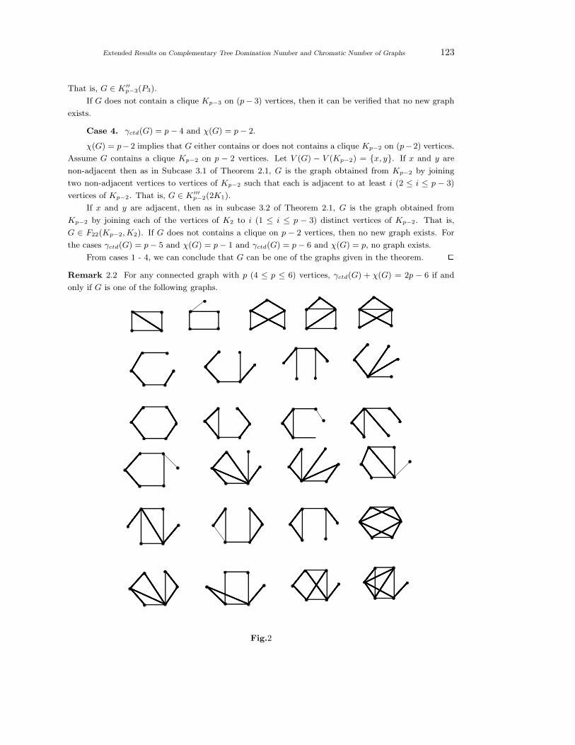
Extended Results on Complementary Tree Domination Number and Chromatic Number of Graphs 123
That is, G ∈ K′′p−3(P3).
If G does not contain a clique Kp−3 on (p− 3) vertices, then it can be verified that no new graph
exists.
Case 4. γctd(G) = p − 4 and χ(G) = p − 2.
χ(G) = p−2 implies that G either contains or does not contains a clique Kp−2 on (p−2) vertices.
Assume G contains a clique Kp−2 on p − 2 vertices. Let V (G) − V (Kp−2) = {x, y}. If x and y are
non-adjacent then as in Subcase 3.1 of Theorem 2.1, G is the graph obtained from Kp−2 by joining
two non-adjacent vertices to vertices of Kp−2 such that each is adjacent to at least i (2 ≤ i ≤ p − 3)
vertices of Kp−2. That is, G ∈ K′′′p−2(2K1).
If x and y are adjacent, then as in subcase 3.2 of Theorem 2.1, G is the graph obtained from
Kp−2 by joining each of the vertices of K2 to i (1 ≤ i ≤ p − 3) distinct vertices of Kp−2. That is,
G ∈ F22(Kp−2, K2). If G does not contains a clique on p − 2 vertices, then no new graph exists. For
the cases γctd(G) = p − 5 and χ(G) = p − 1 and γctd(G) = p − 6 and χ(G) = p, no graph exists.
From cases 1 - 4, we can conclude that G can be one of the graphs given in the theorem. 2Remark 2.2 For any connected graph with p (4 ≤ p ≤ 6) vertices, γctd(G) + χ(G) = 2p − 6 if and
only if G is one of the following graphs.
Fig.2
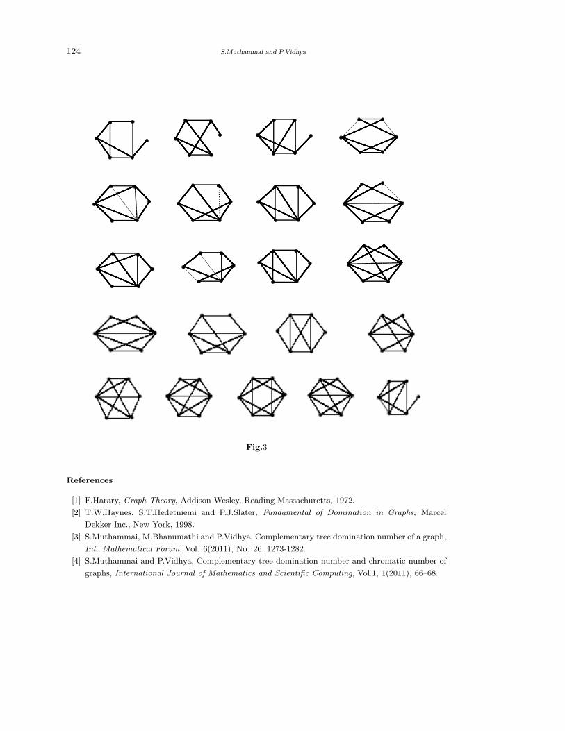
124 S.Muthammai and P.Vidhya
Fig.3
References
[1] F.Harary, Graph Theory, Addison Wesley, Reading Massachuretts, 1972.
[2] T.W.Haynes, S.T.Hedetniemi and P.J.Slater, Fundamental of Domination in Graphs, Marcel
Dekker Inc., New York, 1998.
[3] S.Muthammai, M.Bhanumathi and P.Vidhya, Complementary tree domination number of a graph,
Int. Mathematical Forum, Vol. 6(2011), No. 26, 1273-1282.
[4] S.Muthammai and P.Vidhya, Complementary tree domination number and chromatic number of
graphs, International Journal of Mathematics and Scientific Computing, Vol.1, 1(2011), 66–68.
International J.Math. Combin. Vol.3(2015), 125-133
On Integer Additive Set-Sequential Graphs
N.K.Sudev
Department of Mathematics
Vidya Academy of Science & Technology, Thalakkottukara, Thrissur - 680501, India
K.A.Germina
PG & Research Department of Mathematics
Mary Matha Arts & Science College, Mnanthavady, Wayanad-670645, India)
E-mail:[email protected], [email protected]
Abstract: A set-labeling of a graph G is an injective function f : V (G) → P(X), where
X is a finite set of non-negative integers and a set-indexer of G is a set-labeling such that
the induced function f⊕ : E(G) → P(X) − {∅} defined by f⊕(uv) = f(u)⊕f(v) for every
uv∈E(G) is also injective. A set-indexer f : V (G) → P(X) is called a set-sequential labeling
of G if f⊕(V (G) ∪ E(G)) = P(X) − {∅}. A graph G which admits a set-sequential labeling
is called a set-sequential graph. An integer additive set-labeling is an injective function
f : V (G) → P(N0), N0 is the set of all non-negative integers and an integer additive set-
indexer is an integer additive set-labeling such that the induced function f+ : E(G) → P(N0)
defined by f+(uv) = f(u) + f(v) is also injective. In this paper, we extend the concepts of
set-sequential labeling to integer additive set-labelings of graphs and provide some results
on them.
Key Words: Integer additive set-indexers, set-sequential graphs, integer additive set-
labeling, integer additive set-sequential labeling, integer additive set-sequential graphs.
AMS(2010): 05C78.
§1. Introduction
For all terms and definitions, not defined specifically in this paper, we refer to [4], [5] and [9] and for
more about graph labeling, we refer to [6]. Unless mentioned otherwise, all graphs considered here are
simple, finite and have no isolated vertices.
All sets mentioned in this paper are finite sets of non-negative integers. We denote the cardinality
of a set A by |A|. We denote, by X, the finite ground set of non-negative integers that is used for
set-labeling the elements of G and cardinality of X by n.
The research in graph labeling commenced with the introduction of β-valuations of graphs in [10].
Analogous to the number valuations of graphs, the concepts of set-labelings and set-indexers of graphs
are introduced in [1] as follows.
Let G be a (p, q)-graph. Let X, Y and Z be non-empty sets and P(X), P(Y ) and P(Z) be their
power sets. Then, the functions f : V (G) → P(X), f : E(G) → P(Y ) and f : V (G) ∪ E(G) → P(Z)
are called the set-assignments of vertices, edges and elements of G respectively. By a set-assignment
1Received December 31, 2014, Accepted August 31, 2015.
126 N.K.Sudev and K.A.Germina
of a graph, we mean any one of them. A set-assignment is called a set-labeling or a set-valuation if it
is injective.
A graph with a set-labeling f is denoted by (G, f) and is referred to as a set-labeled graph or
a set-valued graph. For a (p, q)- graph G = (V, E) and a non-empty set X of cardinality n, a set-
indexer of G is defined as an injective set-valued function f : V (G) → P(X) such that the function
f⊕ : E(G) → P(X) − {∅} defined by f⊕(uv) = f(u)⊕f(v) for every uv∈E(G) is also injective, where
P(X) is the set of all subsets of X and ⊕ is the symmetric difference of sets.
Theorem 1.1([1]) Every graph has a set-indexer.
Analogous to graceful labeling of graphs, the concept of set-graceful labeling and set-sequential
labeling of a graph are defined in [1] as follows.
Let G be a graph and let X be a non-empty set. A set-indexer f : V (G) → P(X) is called a
set-graceful labeling of G if f⊕(E(G)) = P(X) − {∅}. A graph G which admits a set-graceful labeling
is called a set-graceful graph.
Let G be a graph and let X be a non-empty set. A set-indexer f : V (G) → P(X) is called a
set-sequential labeling of G if f⊕(V (G)∪E(G)) = P(X)−{∅}. A graph G which admits a set-sequential
labeling is called a set-sequential graph.
Let A and B be two non-empty sets. Then, their sum set, denoted by A + B, is defined to be
the set A + B = {a + b : a ∈ A, b ∈ B}. If C = A + B, then A and B are said to be the summands
of C. Using the concepts of sum sets of sets of non-negative integers, the notion of integer additive
set-labeling of a given graph G is introduced as follows.
Let N0 be the set of all non-negative integers. An integer additive set-labeling (IASL, in short) of
graph G is an injective function f : V (G) → P(N0) such that the induced function f+ : E(G) → P(N0)
is defined by f+(uv) = f(u) + f(v) for ∀uv ∈ E(G). A graph G which admits an IASL is called an
IASL graph.
An integer additive set-labeling f is an integer additive set-indexer (IASI, in short) if the induced
function f+ : E(G) → P(N0) defined by f+(uv) = f(u) + f(v) is injective(see [7]). A graph G which
admits an IASI is called an IASI graph.
The following notions are introduced in [11] and [8]. The cardinality of the set-label of an element
(vertex or edge) of a graph G is called the set-indexing number of that element. An IASL (or an IASI)
is said to be a k-uniform IASL (or k-uniform IASI) if |f+(e)| = k ∀ e ∈ E(G). The vertex set V (G) is
called l-uniformly set-indexed, if all the vertices of G have the set-indexing number l.
Definition 1.2([13]) Let G be a graph and let X be a non-empty set. An integer additive set-indexer
f : V (G) → P(X) − {∅} is called a integer additive set-graceful labeling (IASGL, in short) of G if
f+(E(G)) = P(X)−{∅, {0}}. A graph G which admits an integer additive set-graceful labeling is called
an integer additive set-graceful graph (in short, IASG-graph).
Motivated from the studies made in [2] and [3], in this paper, we extend the concepts of set-
sequential labelings of graphs to integer additive set-sequential labelings and establish some results on
them.
§2. IASSL of Graphs
First, note that under an integer additive set-labeling, no element of a given graph can have ∅ as its
On Integer Additive Set-Sequential Graphs 127
set-labeling. Hence, we need to consider only non-empty subsets of X for set-labeling the elements of
G.
Let f be an integer additive set-indexer of a given graph G. Define a function f∗ : V (G)∪E(G) →P(X) − {∅} as follows.
f∗(x) =
f(x) if x ∈ V (G)
f+(x) if x ∈ E(G)(2.1)
Clearly, f∗[V (G) ∪ E(G)] = f(V (G)) ∪ f+(E(G)). By the notation, f∗(G), we mean f∗[V (G) ∪E(G)]. Then, f∗ is an extension of both f and f+ of G. Throughout our discussions in this paper, the
function f∗ is as per the definition in Equation 2.1.
Using the definition of new induced function f∗ of f , we introduce the following notion as a sum
set analogue of set-sequential graphs.
Definition 2.1 An IASI f of G is said to be an integer additive set-sequential labeling (IASSL) if the
induced function f∗(G) = f(V (G))∪ f+E(G)) = P(X)−{∅}. A graph G which admits an IASSL may
be called an integer additive set-sequential graph (IASS-graph).
Hence, an integer additive set-sequential indexer can be defined as follows.
Definition 2.2 An integer additive set-sequential labeling f of a given graph G is said to be an integer
additive set-sequential indexer (IASSI) if the induced function f∗ is also injective. A graph G which
admits an IASSI may be called an integer additive set-sequential indexed graph (IASSI-graph).
A question that arouses much in this context is about the comparison between an IASGL and an
IASSL of a given graph if they exist. The following theorem explains the relation between an IASGL
and an IASSL of a given graph G.
Theorem 2.3 Every integer additive set-graceful labeling of a graph G is also an integer additive
set-sequential labeling of G.
Proof Let f be an IASGL defined on a given graph G. Then, {0} ∈ f(V (G)) (see [13]) and
|f+(E(G))| = P(X) − {∅, {0}}. Then, f∗(G) contains all non-empty subsets of X. Therefore, f is an
IASSL of G. 2Let us now verify the injectivity of the function f∗ in the following proposition.
Proposition 2.4 Let G be a graph without isolated vertices. If the function f∗ is an injective, then no
vertex of G can have a set-label {0}.Proof If possible let a vertex, say v, has the set-label {0}. Since G is connected, v is adjacent to
at least one vertex in G. Let u be an adjacent vertex of v in G and u has a set-label A ⊂ X. Then,
f∗(u) = f(u) = A and f∗(uv) = f+(uv) = A, which is a contradiction to the hypothesis that f∗ is
injective. 2In view of Observation 2.4, we notice the following points.
Remark 2.5 Suppose that the function f∗ defined in (2.1) is injective. Then, if one vertex v of G has
the set label {0}, then v is an isolated vertex of G.
Remark 2.6 If the function f∗ defined in (2.1) is injective, then no edge of G can also have the set
128 N.K.Sudev and K.A.Germina
label {0}.
The following result is an immediate consequence of the addition theorem on sets in set theory
and provides a relation connecting the size and order of a given IASS-graph G and the cardinality of
its ground set X.
Proposition 2.7 Let G be a graph on n vertices and m edges. If f is an IASSL of a graph G with
respect to a ground set X, then m + n = 2|X| − (1 + κ), where κ is the number of subsets of X which
is the set-label of both a vertex and an edge.
Proof Let f be an IASSL defined on a given graph G. Then, |f∗(G)| = |f(V (G)) ∪ f+(E(G))| =
|P(X) − {∅}| = 2|X| − 1. But by addition theorem on sets, we have
|f∗(G)| = |f(V (G)) ∪ f+(E(G))|That is, 2|X| − 1 = |f(V (G))| + |f+(E(G))| − |f(V (G)) ∩ f+(E(G))|
= |V | + |E| − κ
=⇒ = m + n − κ
Whence m + n = 2|X| − 1 − κ.
This completes the proof. 2We say that two sets A and B are of same parity if their cardinalities are simultaneously odd or
simultaneously even. Then, the following theorem is on the parity of the vertex set and edge set of G.
Proposition 2.8 Let f be an IASSL of a given graph G, with respect to a ground set X. Then, if
V (G) and E(G) are of same parity, then κ is an odd integer and if V (G) and E(G) are of different
parity, then κ is an even integer, where κ is the number of subsets of X which are the set-labels of both
vertices and edges.
Proof Let f be a integer additive set-sequential labeling of a given graph G. Then, f∗(G) =
P(X) − {∅}. Therefore, |f∗(G)| = 2|X| − 1, which is an odd integer.
Case 1. Let V (G) and E(G) are of same parity. Then, |V | + |E| is an even integer. Then, by
Proposition 2.7, 2|X| − 1 − κ is an even integer, which is possible only when κ is an odd integer.
Case 2. Let V (G) and E(G) are of different parity. Then, |V |+ |E| is an odd integer. Then, by
Proposition 2.7, 2|X| − 1 − κ is an odd integer, which is possible only when κ is an even integer. 2A relation between integer additive set-graceful labeling and an integer additive set-sequential
labeling of a graph is established in the following result.
The following result determines the minimum number of vertices in a graph that admits an IASSL
with respect to a finite non-empty set X.
Theorem 2.9 Let X be a non-empty finite set of non-negative integers. Then, a graph G that admits
an IASSL with respect to X have at least ρ vertices, where ρ is the number of elements in P(X) which
are not the sum sets of any two elements of P(X).
Proof Let f be an IASSL of a given graph G, with respect to a given ground set X. Let A be
the collection of subsets of X such that no element in A is the sum sets any two subsets of X. Since f
an IASL of G, all edge of G must have the set-labels which are the sum sets of the set-labels of their
On Integer Additive Set-Sequential Graphs 129
end vertices. Hence, no element in A can be the set-label of any edge of G. But, since f is an IASSL
of G, A ⊂ f∗(G) = f(V (G))∪ f+(E(G)). Therefore, the minimum number of vertices of G is equal to
the number of elements in the set A. 2The structural properties of graphs which admit IASSLs arouse much interests. In the example of
IASS-graphs, given in Figure 1, the graph G has some pendant vertices. Hence, there arises following
questions in this context. Do an IASS-graph necessarily have pendant vertices? If so, what is the
number of pendant vertices required for a graph G to admit an IASSL? Let us now proceed to find the
solutions to these problems.
The minimum number of pendant vertices required in a given IASS-graph is explained in the
following Theorem.
Theorem 2.10 Let G admits an IASSL with respect to a ground set X and let B be the collection of
subsets of X which are neither the sum sets of any two subsets of X nor their sum sets are subsets of
X. If B is non-empty, then
(1) {0} is the set-label of a vertex in G;
(2) the minimum number pendant vertices in G is cardinality of B.
Remark 2.11 Since the ground set X of an IASS-graph must contain the element 0, every subset Ai
of X sum set of {0} and Ai itself. In this sense, each subset Ai may be considered as a trivial sum set
of two subsets of X.
In the following discussions, by a sum set of subsets of X, we mean the non-trivial sum sets of
subsets of X.
Proof Let f be an IASSL of G with respect to a ground set X. Also, let B be the collection of
subsets of X which are neither the sum sets of any two subsets of X nor their sum sets are subsets
of X. Let A ⊂ X be an element of B. then A must be the set-label of a vertex of G. Since A ∈ B,
the only set that can be adjacent to A is {0}. Therefore, since G is a connected graph, {0} must be
the set-label of a vertex of G. More over, since A is an arbitrary vertex in B, the minimum number of
pendant vertices in G is |B|. 2The following result thus establishes the existence of pendant vertices in an IASS-graph.
Theorem 2.12 Every graph that admits an IASSL, with respect to a non-empty finite ground set X,
have at least one pendant vertex.
Proof Let the graph G admits an IASSL f with respect to a ground set X. Let B be the collection
of subsets of X which are neither the sum sets of any two subsets of X nor their sum sets are subsets
of X.
We claim that B is non-empty, which can be proved as follows. Since X is a finite set of non-
negative integers, X has a smallest element, say x1, and a greatest element xl. Then, the subset
{x1, xl} belongs to f∗(G). Since it is not the sum set any sets and is not a summand of any set in
P(X), {x1, xl} ∈ B. Therefore, B is non-empty.
Since B is non-empty, by Theorem 2.10, G has some pendant vertices. 2Remark 2.13 In view of the above results, we can make the following observations.
(1) No cycle Cn can have an IASSL;
(2) For n > 2, no complete graph Kn admits an IASSL.
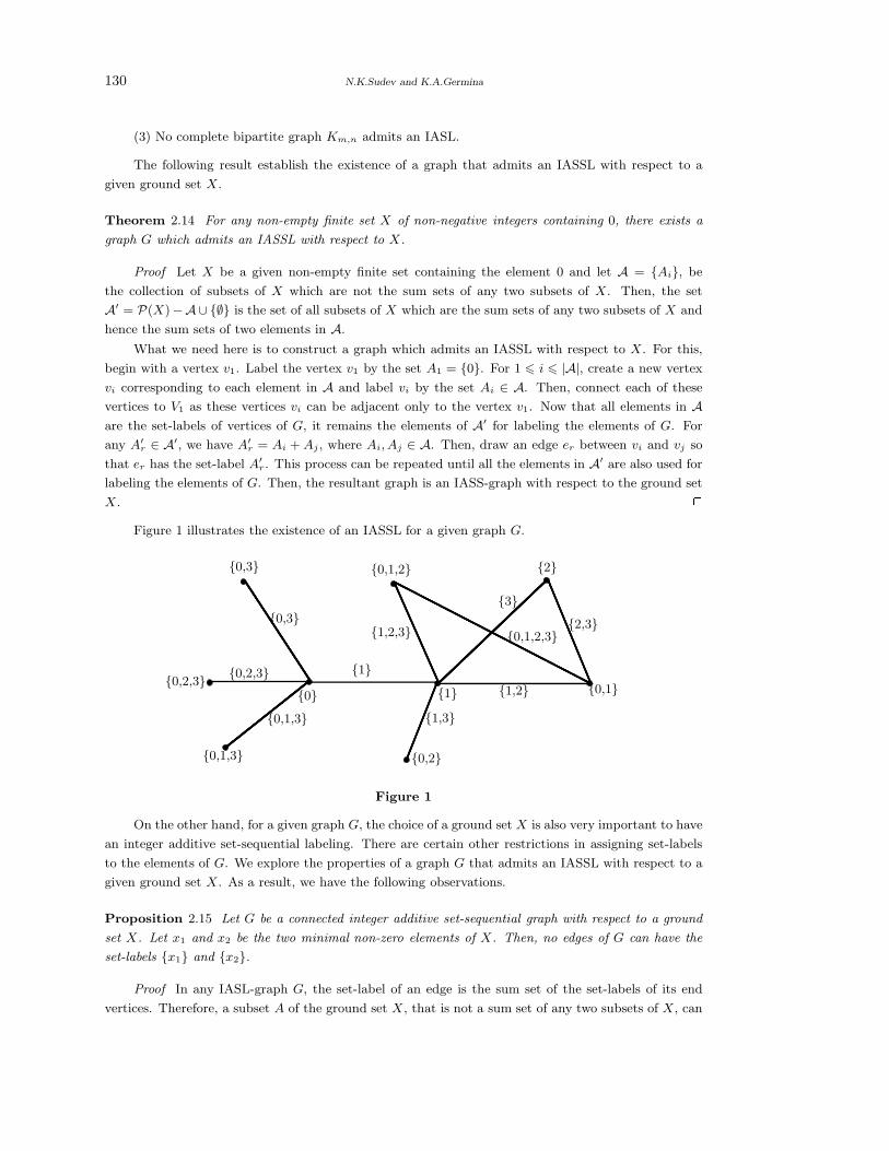
130 N.K.Sudev and K.A.Germina
(3) No complete bipartite graph Km,n admits an IASL.
The following result establish the existence of a graph that admits an IASSL with respect to a
given ground set X.
Theorem 2.14 For any non-empty finite set X of non-negative integers containing 0, there exists a
graph G which admits an IASSL with respect to X.
Proof Let X be a given non-empty finite set containing the element 0 and let A = {Ai}, be
the collection of subsets of X which are not the sum sets of any two subsets of X. Then, the set
A′ = P(X)−A∪ {∅} is the set of all subsets of X which are the sum sets of any two subsets of X and
hence the sum sets of two elements in A.
What we need here is to construct a graph which admits an IASSL with respect to X. For this,
begin with a vertex v1. Label the vertex v1 by the set A1 = {0}. For 1 6 i 6 |A|, create a new vertex
vi corresponding to each element in A and label vi by the set Ai ∈ A. Then, connect each of these
vertices to V1 as these vertices vi can be adjacent only to the vertex v1. Now that all elements in Aare the set-labels of vertices of G, it remains the elements of A′ for labeling the elements of G. For
any A′r ∈ A′, we have A′
r = Ai + Aj , where Ai, Aj ∈ A. Then, draw an edge er between vi and vj so
that er has the set-label A′r. This process can be repeated until all the elements in A′ are also used for
labeling the elements of G. Then, the resultant graph is an IASS-graph with respect to the ground set
X. 2Figure 1 illustrates the existence of an IASSL for a given graph G.
{0,3}
{0}
{0,2}
{1,3}{1} {0,1}{1,2}
{1,2,3}
{0,1,2} {2}
{2,3}{3}
{0,1,2,3}{0,3}
{0,1,3}
{1}{0,2,3}
{0,1,3}
{0,2,3}
Figure 1
On the other hand, for a given graph G, the choice of a ground set X is also very important to have
an integer additive set-sequential labeling. There are certain other restrictions in assigning set-labels
to the elements of G. We explore the properties of a graph G that admits an IASSL with respect to a
given ground set X. As a result, we have the following observations.
Proposition 2.15 Let G be a connected integer additive set-sequential graph with respect to a ground
set X. Let x1 and x2 be the two minimal non-zero elements of X. Then, no edges of G can have the
set-labels {x1} and {x2}.
Proof In any IASL-graph G, the set-label of an edge is the sum set of the set-labels of its end
vertices. Therefore, a subset A of the ground set X, that is not a sum set of any two subsets of X, can
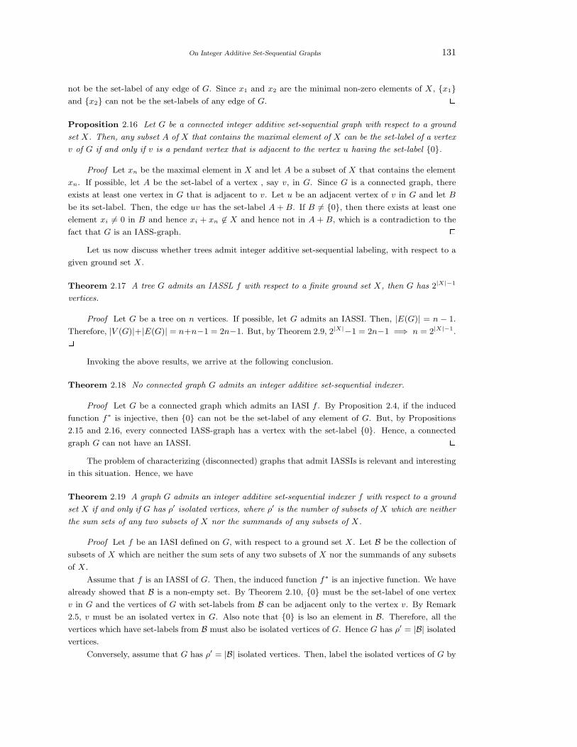
On Integer Additive Set-Sequential Graphs 131
not be the set-label of any edge of G. Since x1 and x2 are the minimal non-zero elements of X, {x1}and {x2} can not be the set-labels of any edge of G. 2Proposition 2.16 Let G be a connected integer additive set-sequential graph with respect to a ground
set X. Then, any subset A of X that contains the maximal element of X can be the set-label of a vertex
v of G if and only if v is a pendant vertex that is adjacent to the vertex u having the set-label {0}.
Proof Let xn be the maximal element in X and let A be a subset of X that contains the element
xn. If possible, let A be the set-label of a vertex , say v, in G. Since G is a connected graph, there
exists at least one vertex in G that is adjacent to v. Let u be an adjacent vertex of v in G and let B
be its set-label. Then, the edge uv has the set-label A + B. If B 6= {0}, then there exists at least one
element xi 6= 0 in B and hence xi + xn 6∈ X and hence not in A + B, which is a contradiction to the
fact that G is an IASS-graph. 2Let us now discuss whether trees admit integer additive set-sequential labeling, with respect to a
given ground set X.
Theorem 2.17 A tree G admits an IASSL f with respect to a finite ground set X, then G has 2|X|−1
vertices.
Proof Let G be a tree on n vertices. If possible, let G admits an IASSI. Then, |E(G)| = n − 1.
Therefore, |V (G)|+|E(G)| = n+n−1 = 2n−1. But, by Theorem 2.9, 2|X|−1 = 2n−1 =⇒ n = 2|X|−1.2Invoking the above results, we arrive at the following conclusion.
Theorem 2.18 No connected graph G admits an integer additive set-sequential indexer.
Proof Let G be a connected graph which admits an IASI f . By Proposition 2.4, if the induced
function f∗ is injective, then {0} can not be the set-label of any element of G. But, by Propositions
2.15 and 2.16, every connected IASS-graph has a vertex with the set-label {0}. Hence, a connected
graph G can not have an IASSI. 2The problem of characterizing (disconnected) graphs that admit IASSIs is relevant and interesting
in this situation. Hence, we have
Theorem 2.19 A graph G admits an integer additive set-sequential indexer f with respect to a ground
set X if and only if G has ρ′ isolated vertices, where ρ′ is the number of subsets of X which are neither
the sum sets of any two subsets of X nor the summands of any subsets of X.
Proof Let f be an IASI defined on G, with respect to a ground set X. Let B be the collection of
subsets of X which are neither the sum sets of any two subsets of X nor the summands of any subsets
of X.
Assume that f is an IASSI of G. Then, the induced function f∗ is an injective function. We have
already showed that B is a non-empty set. By Theorem 2.10, {0} must be the set-label of one vertex
v in G and the vertices of G with set-labels from B can be adjacent only to the vertex v. By Remark
2.5, v must be an isolated vertex in G. Also note that {0} is lso an element in B. Therefore, all the
vertices which have set-labels from B must also be isolated vertices of G. Hence G has ρ′ = |B| isolated
vertices.
Conversely, assume that G has ρ′ = |B| isolated vertices. Then, label the isolated vertices of G by
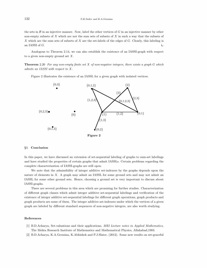
132 N.K.Sudev and K.A.Germina
the sets in B in an injective manner. Now, label the other vertices of G in an injective manner by other
non-empty subsets of X which are not the sum sets of subsets of X in such a way that the subsets of
X which are the sum sets of subsets of X are the set-labels of the edges of G. Clearly, this labeling is
an IASSI of G. 2Analogous to Theorem 2.14, we can also establish the existence of an IASSI-graph with respect
to a given non-empty ground set X.
Theorem 2.20 For any non-empty finite set X of non-negative integers, there exists a graph G which
admits an IASSI with respect to X.
Figure 2 illustrates the existence of an IASSL for a given graph with isolated vertices.
{0,3}
{0,2}
{1,3}{1} {0,1}{1,2}
{1,2,3}
{0,1,2} {2}
{2,3}{3}
{0,1,2,3}
{0,2,3}
{0,1,3}
{0}
Figure 2
§3. Conclusion
In this paper, we have discussed an extension of set-sequential labeling of graphs to sum-set labelings
and have studied the properties of certain graphs that admit IASSLs. Certain problems regarding the
complete characterization of IASSI-graphs are still open.
We note that the admissibility of integer additive set-indexers by the graphs depends upon the
nature of elements in X. A graph may admit an IASSL for some ground sets and may not admit an
IASSL for some other ground sets. Hence, choosing a ground set is very important to discuss about
IASSI-graphs.
There are several problems in this area which are promising for further studies. Characterization
of different graph classes which admit integer additive set-sequential labelings and verification of the
existence of integer additive set-sequential labelings for different graph operations, graph products and
graph products are some of them. The integer additive set-indexers under which the vertices of a given
graph are labeled by different standard sequences of non-negative integers, are also worth studying.
References
[1] B.D.Acharya, Set-valuations and their applications, MRI Lecture notes in Applied Mathematics,
The Mehta Research Institute of Mathematics and Mathematical Physics, Allahabad,1983.
[2] B.D.Acharya, K.A.Germina, K.Abhishek and P.J.Slater, (2012). Some new results on set-graceful
On Integer Additive Set-Sequential Graphs 133
and set-sequential graphs, Journal of Combinatorics, Information and System Sciences, 37(2-4),
145-155.
[3] B.D.Acharya and S.M.Hegde, Set-Sequential Graphs, National Academy Science Letters, 8(12)(1985),
387-390.
[4] J.A.Bondy and U.S.R.Murty, Graph Theory, Springer, 2008.
[5] A.Brandstadt, V.B.Le and J.P.Spinard, Graph Classes:A Survey, SIAM, Philadelphia, (1999).
[6] J.A.Gallian, A dynamic survey of graph labelling, The Electronic Journal of Combinatorics, (DS-
6), (2013).
[7] K.A.Germina and T.M.K.Anandavally, Integer additive set-indexers of a graph: sum square graphs,
Journal of Combinatorics, Information and System Sciences, 37(2-4)(2012), 345-358.
[8] K.A.Germina and N.K.Sudev, On weakly uniform integer additive set-indexers of graphs, Inter-
national Mathematical Forum, 8(37)(2013), 1827-1834.
[9] F.Harary, Graph Theory, Addison-Wesley Publishing Company Inc., 1969.
[10] A.Rosa, On certain valuation of the vertices of a graph, In Theory of Graphs, Gordon and Breach,
(1967).
[11] N.K.Sudev and K.A.Germina, On integer additive set-indexers of graphs, International Journal
of Mathematical Sciences & Engineering Applications, 8(2)(2014), 11-22.
[12] N.K.Sudev and K.A.Germina, Some new results on strong integer additive set-indexers of graphs,
Discrete Mathematics, Algorithms & Applications, 7(1)(2015), 1-11.
[13] N.K.Sudev and K.A.Germina, A study on integer additive set-graceful labelings of graphs, to
appear.
[14] N.K.Sudev, K.A.Germina and K.P Chithra, A creative review on integer additive set-valued
graphs, International Journal of Scientific and Engineering Research, 6(3)(2015), 372-378.
[15] D. B. West, An Introduction to Graph Theory, Pearson Education, 2001.

In silence, in steadiness, in severe abstraction, let him hold by himself, addobservation to observation, patient of neglect, patient of reproach , and bide hisown time , happy enough if he can satisfy himself alone that the day he has seensomething truly.
By Ralph Waldo Emerson, an American thinker.
Author Information
Submission: Papers only in electronic form are considered for possible publication. Papers prepared
in formats, viz., .tex, .dvi, .pdf, or.ps may be submitted electronically to one member of the Editorial
Board for consideration in the International Journal of Mathematical Combinatorics (ISSN
1937-1055). An effort is made to publish a paper duly recommended by a referee within a period of 3
months. Articles received are immediately put the referees/members of the Editorial Board for their
opinion who generally pass on the same in six week’s time or less. In case of clear recommendation
for publication, the paper is accommodated in an issue to appear next. Each submitted paper is not
returned, hence we advise the authors to keep a copy of their submitted papers for further processing.
Abstract: Authors are requested to provide an abstract of not more than 250 words, latest Mathemat-
ics Subject Classification of the American Mathematical Society, Keywords and phrases. Statements
of Lemmas, Propositions and Theorems should be set in italics and references should be arranged in
alphabetical order by the surname of the first author in the following style:
Books
[4]Linfan Mao, Combinatorial Geometry with Applications to Field Theory, InfoQuest Press, 2009.
[12]W.S.Massey, Algebraic topology: an introduction, Springer-Verlag, New York 1977.
Research papers
[6]Linfan Mao, Mathematics on non-mathematics - A combinatorial contribution, International J.Math.
Combin., Vol.3(2014), 1-34.
[9]Kavita Srivastava, On singular H-closed extensions, Proc. Amer. Math. Soc. (to appear).
Figures: Figures should be drawn by TEXCAD in text directly, or as EPS file. In addition, all figures
and tables should be numbered and the appropriate space reserved in the text, with the insertion point
clearly indicated.
Copyright: It is assumed that the submitted manuscript has not been published and will not be
simultaneously submitted or published elsewhere. By submitting a manuscript, the authors agree that
the copyright for their articles is transferred to the publisher, if and when, the paper is accepted for
publication. The publisher cannot take the responsibility of any loss of manuscript. Therefore, authors
are requested to maintain a copy at their end.
Proofs: One set of galley proofs of a paper will be sent to the author submitting the paper, un-
less requested otherwise, without the original manuscript, for corrections after the paper is accepted
for publication on the basis of the recommendation of referees. Corrections should be restricted to
typesetting errors. Authors are advised to check their proofs very carefully before return.
September 2015
Contents
A Calculus and Algebra Derived from Directed Graph Algebras
By Kh.Shahbazpour and Mahdihe Nouri . . . . . . . . . . . . . . . . . . . . . . . . . . . . . . . . . . . . . . . . . . . . . . . . . . . . . 01
Superior Edge Bimagic Labelling
By R.Jagadesh and J.Baskar Babujee . . . . . . . . . . . . . . . . . . . . . . . . . . . . . . . . . . . . . . . . . . . . . . . . . . . . . . . . 33
Spherical Images of Special Smarandache Curves in E3
By Vahide Bulut and Ali Caliskan . . . . . . . . . . . . . . . . . . . . . . . . . . . . . . . . . . . . . . . . . . . . . . . . . . . . . . . . . . . 43
Variations of Orthogonality of Latin Squares
By Vadiraja Bhatta G.R. and B.R.Shankar. . . . . . . . . . . . . . . . . . . . . . . . . . . . . . . . . . . . . . . . . . . . . . . . . . .55
The Minimum Equitable Domination Energy of a Graph
By P.Rajendra and R.Rangarajan . . . . . . . . . . . . . . . . . . . . . . . . . . . . . . . . . . . . . . . . . . . . . . . . . . . . . . . . . . . . 62
Some Results on Relaxed Mean Labeling
By V.Maheswari, D.S.T.Ramesh and V.Balaji . . . . . . . . . . . . . . . . . . . . . . . . . . . . . . . . . . . . . . . . . . . . . . . . 73
Split Geodetic Number of a Line Graph
By Venkanagouda M Goudar and Ashalatha K.S . . . . . . . . . . . . . . . . . . . . . . . . . . . . . . . . . . . . . . . . . . . . . 81
Skolem Difference Odd Mean Labeling For Some Simple Graphs
By R.Vasuki, J.Venkateswari and G.Pooranam . . . . . . . . . . . . . . . . . . . . . . . . . . . . . . . . . . . . . . . . . . . . . . . 88
Radio Number for Special Family of Graphs with Diameter 2, 3 and 4
By M.Murugan . . . . . . . . . . . . . . . . . . . . . . . . . . . . . . . . . . . . . . . . . . . . . . . . . . . . . . . . . . . . . . . . . . . . . . . . . . . . . . 99
Vertex-to-Edge-set Distance Neighborhood Pattern Matrices
By Kishori P.Narayankar and Lokesh S. B. . . . . . . . . . . . . . . . . . . . . . . . . . . . . . . . . . . . . . . . . . . . . . . . . . . 105
Extended Results on Complementary Tree Domination Number and
Chromatic Number of Graphs By S.Muthammai and P.Vidhya . . . . . . . . . . . . . . . . . . . . . . . 116
On Integer Additive Set-Sequential Graphs
By N.K.Sudev and K.A.Germina . . . . . . . . . . . . . . . . . . . . . . . . . . . . . . . . . . . . . . . . . . . . . . . . . . . . . . . . . . . 125
An International Journal on Mathematical Combinatorics