Embed Size (px)
Citation preview

Mathematical Foundations of Data Analysis (MFDA) - II
Boqiang Huang
Institute of Mathematics, University of Cologne, Germany
2019.04.09-11
Chapter 1. Basics
❖ 1. Probablity and Information Theory
1.1. Basic defintions and rules in probability theory
1.2. Basic definitons and rules in information theory
2.1 Basic knowledge in numerical computation
❖ 2. Numerical computation
2.2 Basic knowledge in optimizations
2.2.1 Gradient-based optimization
2.2.2 Constrained optimization
❖ 3. Application: statitical model based data denoising (in tutorial after lecture this Thursday)
Reference:
[1] I. Goodfellow, Y. Bengio, A. Courville, Deep learning, Chapter 3-4, MIT Press, 2016.
[2] A. Antoniou, W.-S. Lu, Practical optimization: algorithms and engineering applications, Springer, 2007.
[3] I. Cohen, Noise spectrum estimation in adverse environments: improved minima controlled recursive averaging, IEEE
Trans. Acoust., Speech, Signal Processing, vol. 11, no. 5, pp. 466-475, 2003.
2019.04.09-11

1. Probablity and Information Theory
❖ Why probability?
Uncertainty and stochasticity can arise from many sources
a. Inherent stochasticity in the system being modeled
2019.04.09-11
e.g. dynamics of subatomic particles, quantum mechanics, other random dynamics
Brownian motion - Wikipedia
1. Probablity and Information Theory
❖ Why probability?
Uncertainty and stochasticity can arise from many sources
a. Inherent stochasticity in the system being modeled
2019.04.09-11
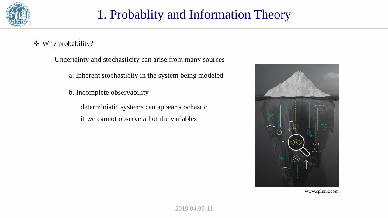
b. Incomplete observability
www.splunk.com
deterministic systems can appear stochastic
if we cannot observe all of the variables
1. Probablity and Information Theory
❖ Why probability?
Uncertainty and stochasticity can arise from many sources
a. Inherent stochasticity in the system being modeled
2019.04.09-11
b. Incomplete observability
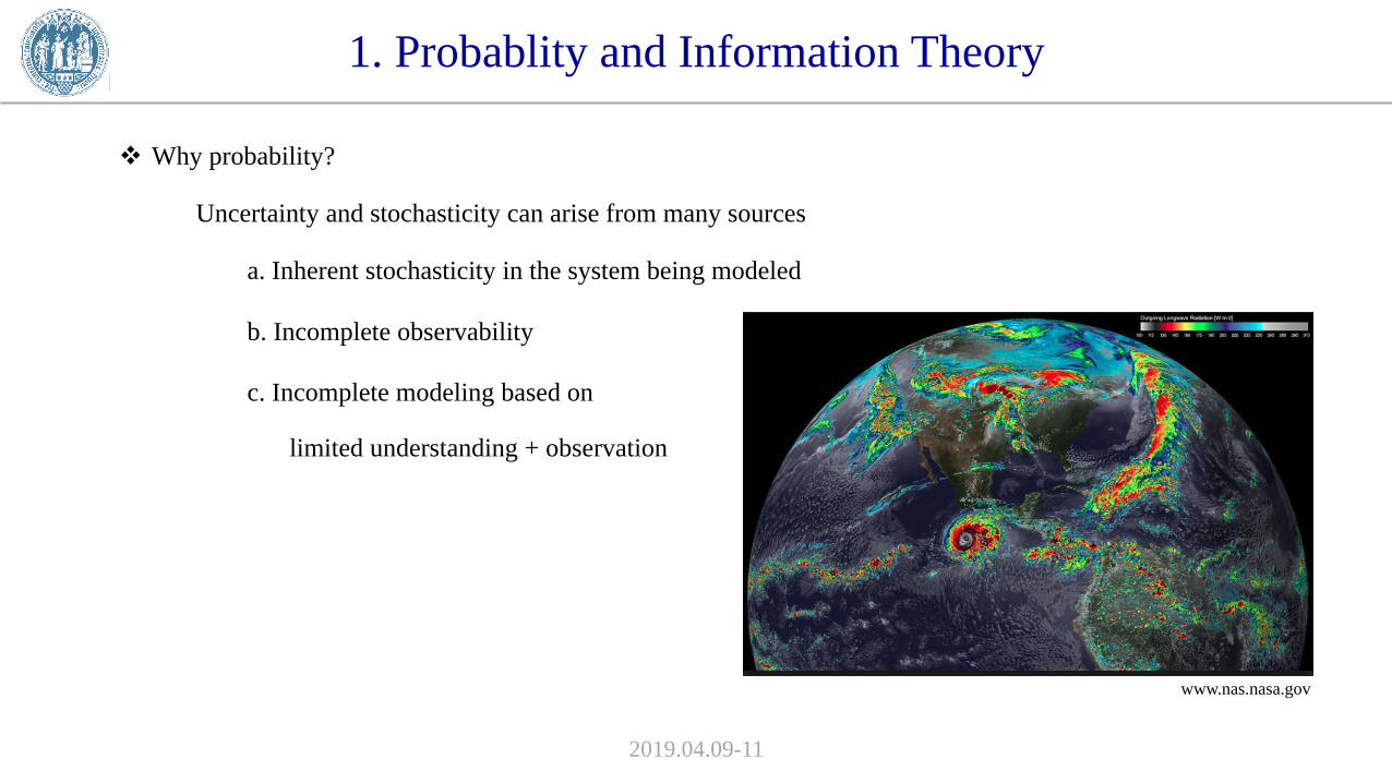
c. Incomplete modeling based on
www.nas.nasa.gov
limited understanding + observation

1. Probablity and Information Theory
❖ Why probability?
Uncertainty and stochasticity can arise from many sources
a. Inherent stochasticity in the system being modeled
2019.04.09-11
b. Incomplete observability
c. Incomplete modeling based on limited understanding + observation
❖ Why information theory?
Quantify, store and communicate the uncertainties, applied in
a. Communication theory, channel coding, data compression, …
b. Gambling, forecasting, investing, …
c. Bioinformatics, astronomy, ...
1. Probablity and Information Theory
1.1 Probability
1.1.1 Random variables
A variable that can take on different values randomly
2019.04.09-11
Random variable as x might be possible state as 𝑥1 or 𝑥2 in scalar or as x in vector
Random variables may be discrete or continuous
1. Probablity and Information Theory
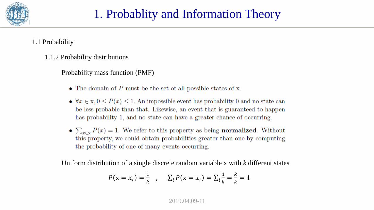
1.1 Probability
1.1.2 Probability distributions
Probability mass function (PMF)
2019.04.09-11
Uniform distribution of a single discrete random variable x with k different states
𝑃 x = 𝑥𝑖 =1
𝑘, σ𝑖 𝑃 x = 𝑥𝑖 = σ𝑖
1
𝑘=
𝑘
𝑘= 1
1. Probablity and Information Theory
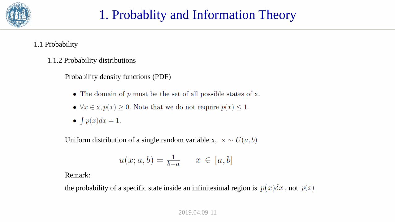
1.1 Probability
1.1.2 Probability distributions
Probability density functions (PDF)
2019.04.09-11
Uniform distribution of a single random variable x,
Remark:
the probability of a specific state inside an infinitesimal region is , not
1. Probablity and Information Theory
1.1 Probability
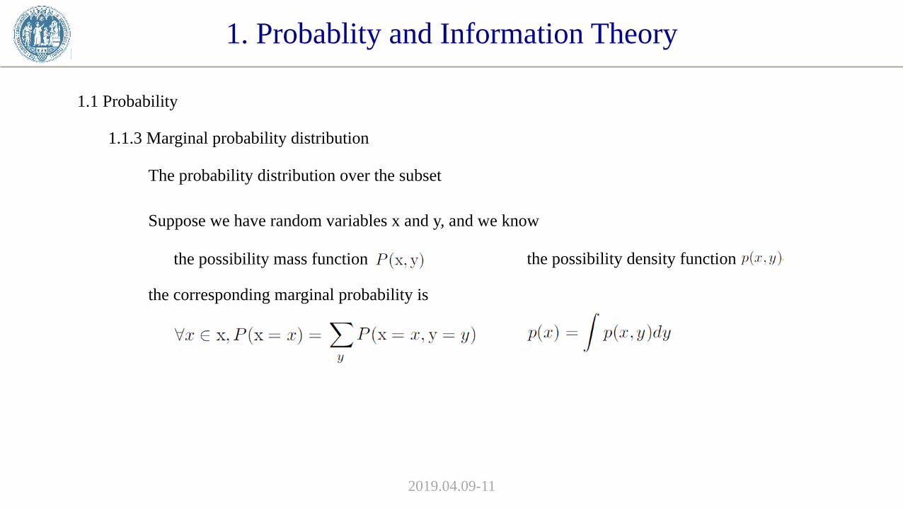
1.1.3 Marginal probability distribution
The probability distribution over the subset
2019.04.09-11
Suppose we have random variables x and y, and we know
the possibility mass function the possibility density function
the corresponding marginal probability is
1. Probablity and Information Theory
1.1 Probability
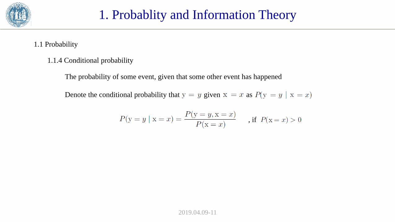
1.1.4 Conditional probability
The probability of some event, given that some other event has happened
2019.04.09-11
Denote the conditional probability that given as
, if
1. Probablity and Information Theory
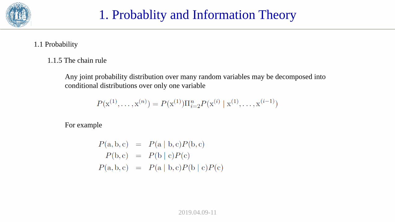
1.1 Probability
1.1.5 The chain rule
Any joint probability distribution over many random variables may be decomposed into
conditional distributions over only one variable
2019.04.09-11
For example
1. Probablity and Information Theory
1.1 Probability
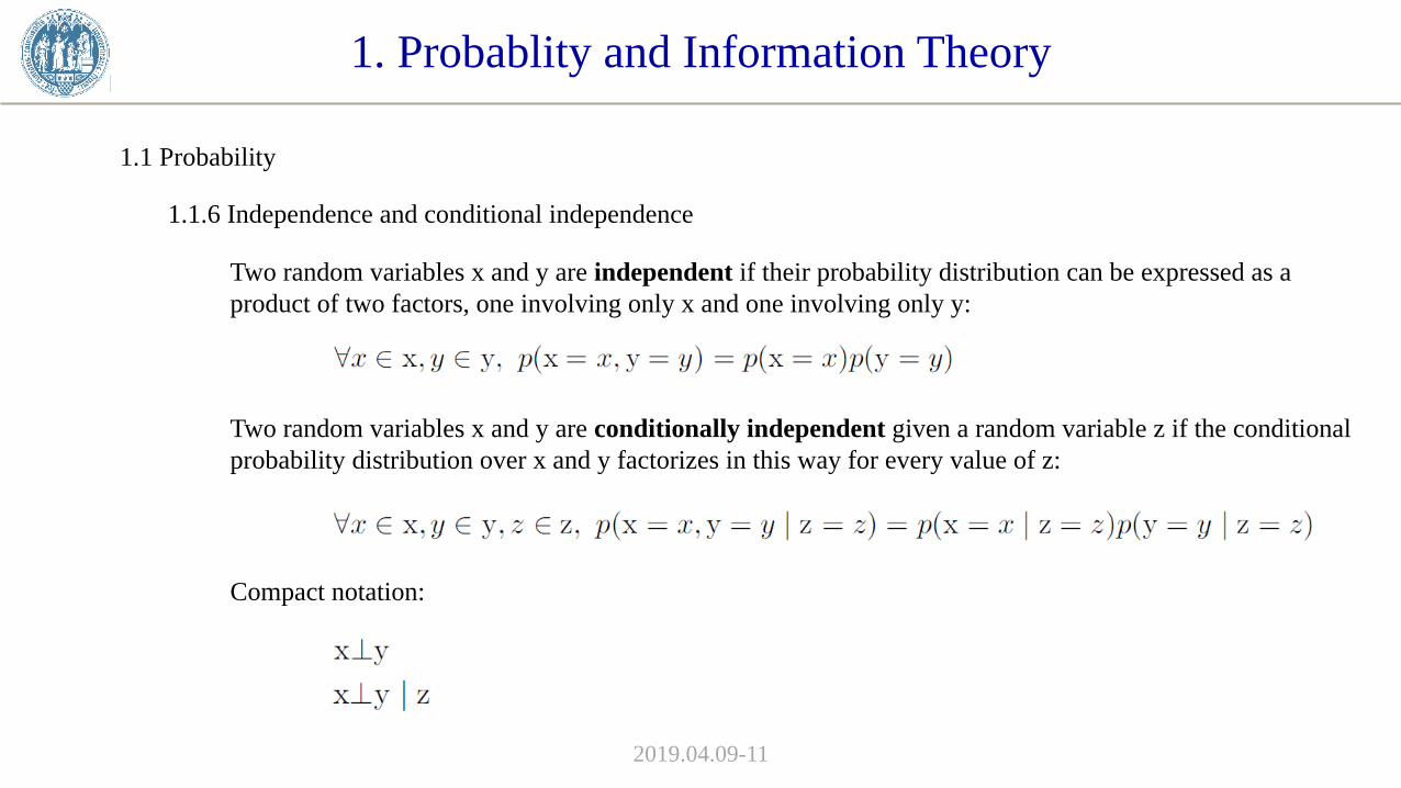
1.1.6 Independence and conditional independence
Two random variables x and y are independent if their probability distribution can be expressed as a
product of two factors, one involving only x and one involving only y:
2019.04.09-11
Two random variables x and y are conditionally independent given a random variable z if the conditional
probability distribution over x and y factorizes in this way for every value of z:
Compact notation:
1. Probablity and Information Theory
1.1 Probability
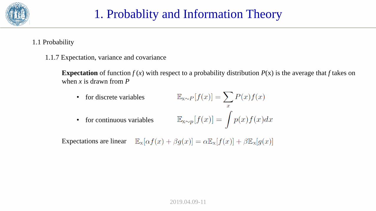
1.1.7 Expectation, variance and covariance
Expectation of function f (x) with respect to a probability distribution P(x) is the average that f takes on
when x is drawn from P
2019.04.09-11
• for discrete variables
• for continuous variables
Expectations are linear
1. Probablity and Information Theory
1.1 Probability
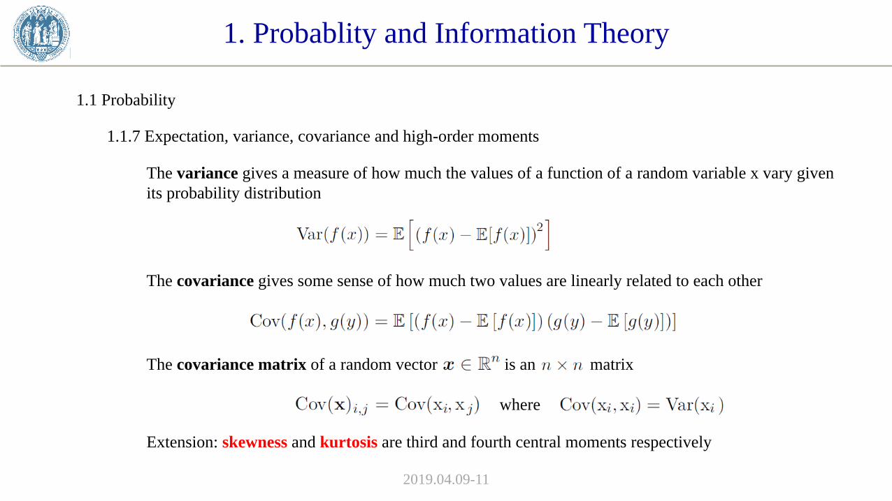
1.1.7 Expectation, variance, covariance and high-order moments
The variance gives a measure of how much the values of a function of a random variable x vary given
its probability distribution
2019.04.09-11
The covariance gives some sense of how much two values are linearly related to each other
The covariance matrix of a random vector is an matrix
where
Extension: skewness and kurtosis are third and fourth central moments respectively
1. Probablity and Information Theory
1.1 Probability
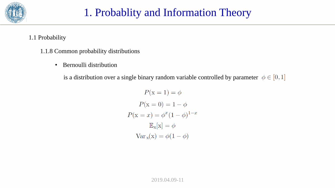
1.1.8 Common probability distributions
• Bernoulli distribution
2019.04.09-11
is a distribution over a single binary random variable controlled by parameter
1. Probablity and Information Theory
1.1 Probability
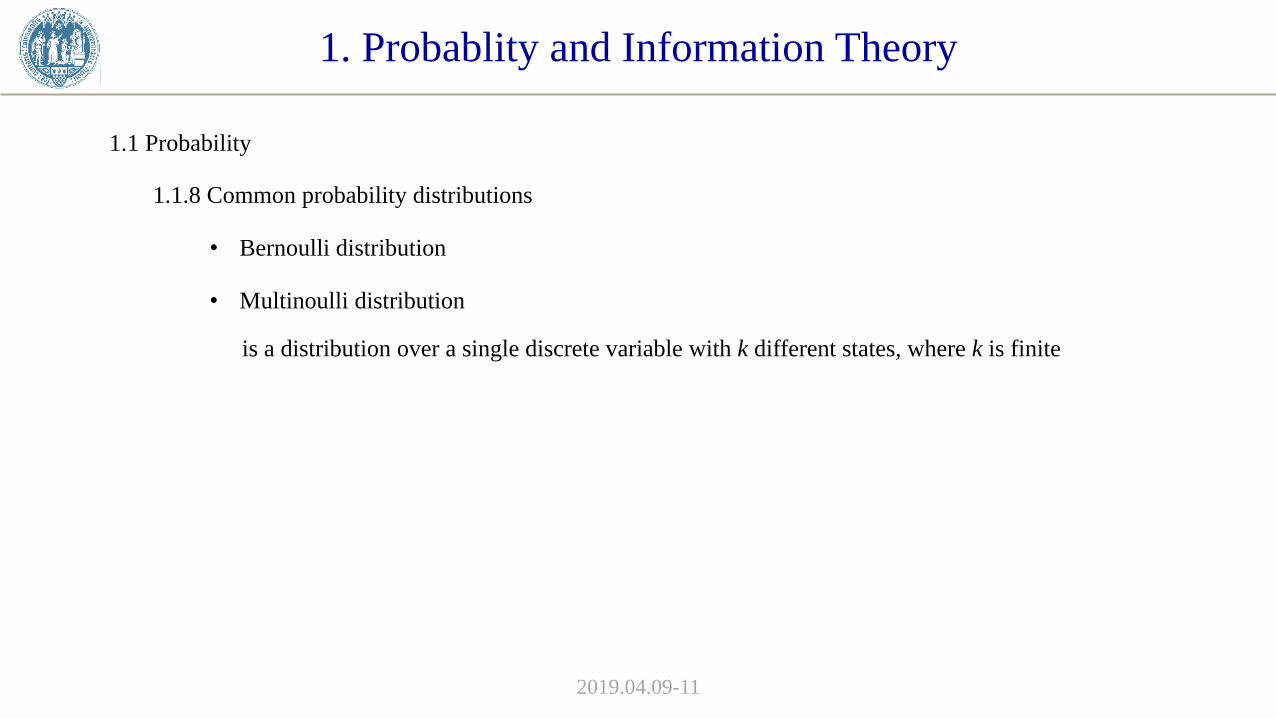
1.1.8 Common probability distributions
• Bernoulli distribution
2019.04.09-11
• Multinoulli distribution
is a distribution over a single discrete variable with k different states, where k is finite
1. Probablity and Information Theory
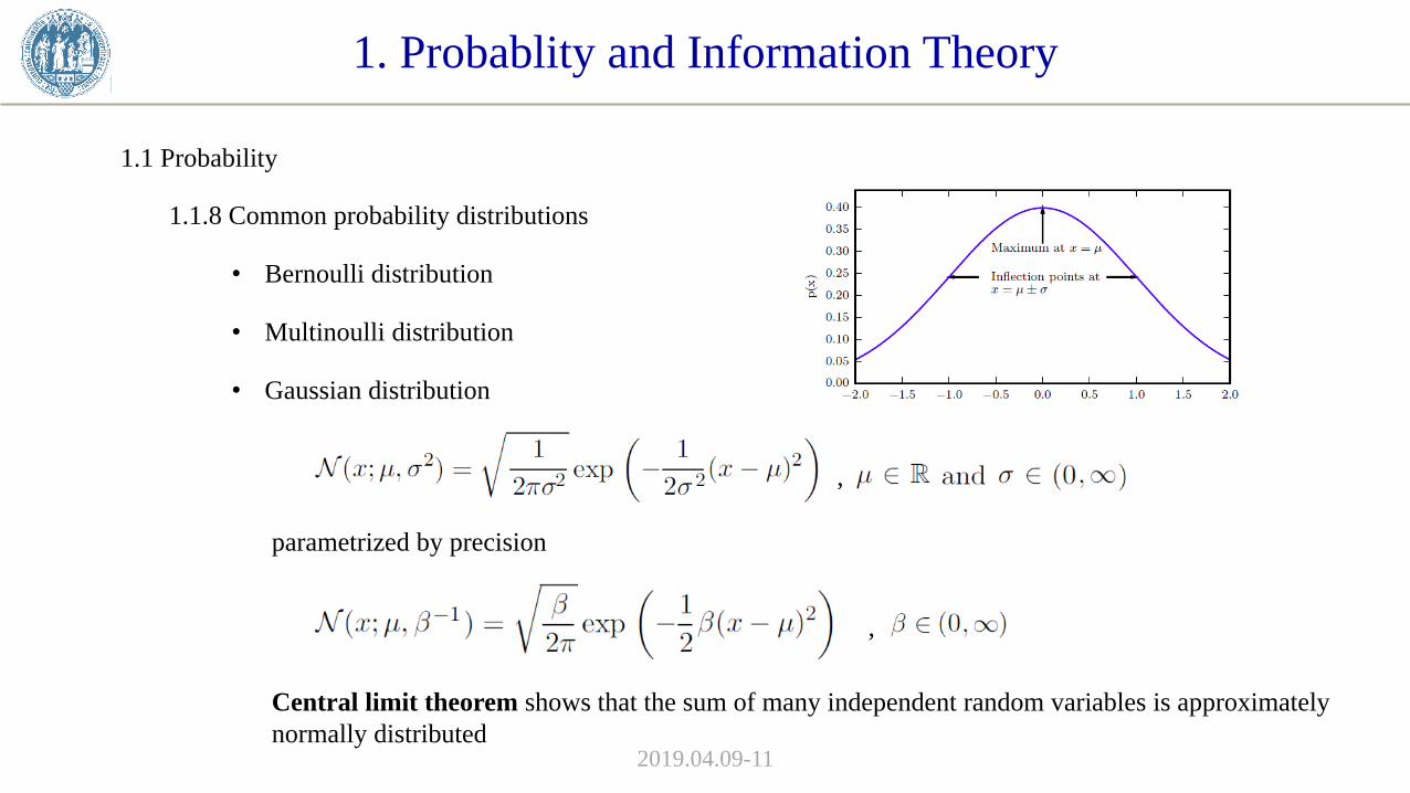
1.1 Probability
1.1.8 Common probability distributions
• Bernoulli distribution
2019.04.09-11
• Multinoulli distribution
• Gaussian distribution
,
parametrized by precision
,
Central limit theorem shows that the sum of many independent random variables is approximately
normally distributed

1. Probablity and Information Theory
1.1 Probability
1.1.8 Common probability distributions
• Bernoulli distribution
2019.04.09-11
• Multinoulli distribution
• Gaussian distribution
,
Multivariate normal distribution
Central limit theorem shows that the sum of many independent random variables is approximately
normally distributed
1. Probablity and Information Theory
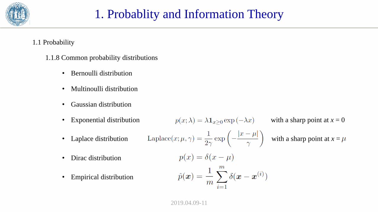
1.1 Probability
1.1.8 Common probability distributions
• Bernoulli distribution
2019.04.09-11
• Multinoulli distribution
• Gaussian distribution
• Exponential distribution with a sharp point at x = 0
• Laplace distribution with a sharp point at x =
• Dirac distribution
• Empirical distribution
1. Probablity and Information Theory
1.1 Probability
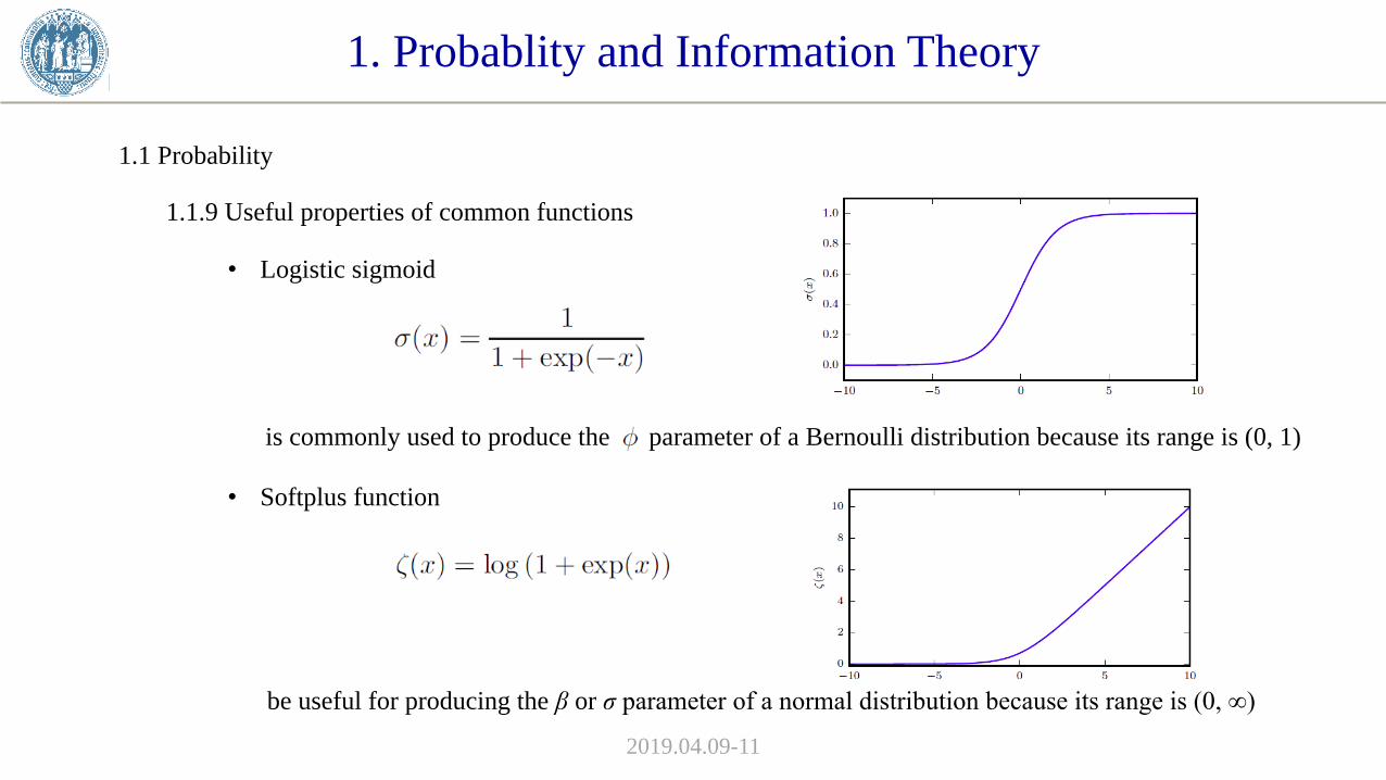
1.1.9 Useful properties of common functions
2019.04.09-11
• Logistic sigmoid
is commonly used to produce the parameter of a Bernoulli distribution because its range is (0, 1)
• Softplus function
be useful for producing the β or σ parameter of a normal distribution because its range is (0, ∞)
1. Probablity and Information Theory
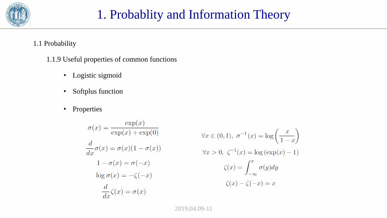
1.1 Probability
1.1.9 Useful properties of common functions
2019.04.09-11
• Logistic sigmoid
• Softplus function
• Properties
1. Probablity and Information Theory
1.1 Probability
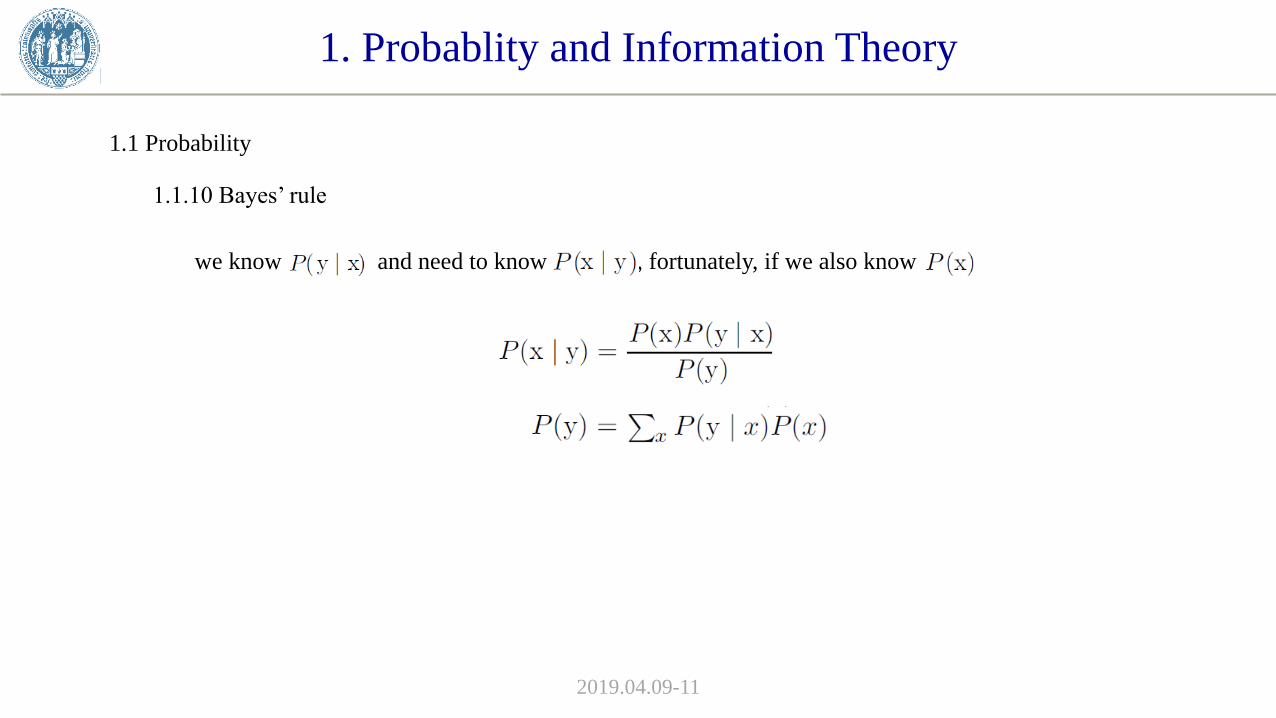
1.1.10 Bayes’ rule
2019.04.09-11
we know and need to know , fortunately, if we also know
1. Probablity and Information Theory
1.2 Information Theory
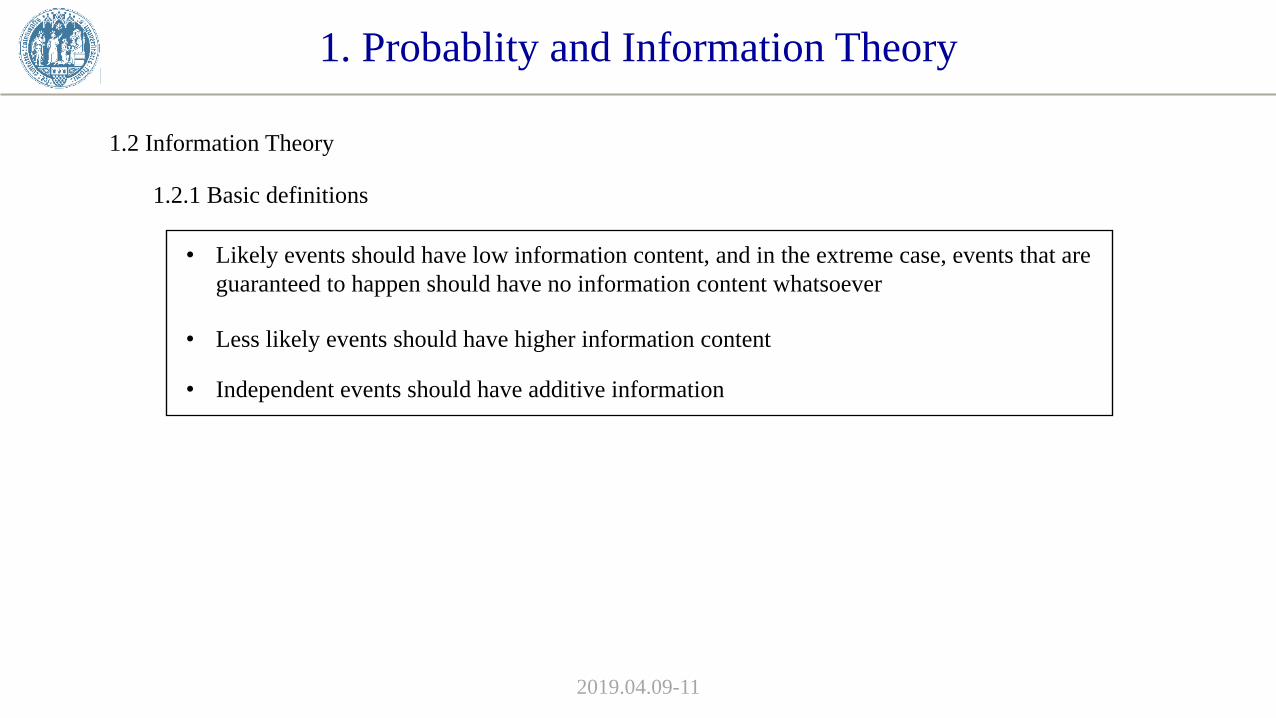
1.2.1 Basic definitions
2019.04.09-11
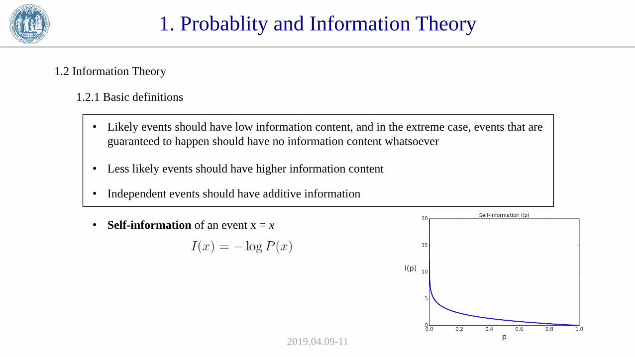
• Likely events should have low information content, and in the extreme case, events that are
guaranteed to happen should have no information content whatsoever
• Less likely events should have higher information content
• Independent events should have additive information
1. Probablity and Information Theory
1.2 Information Theory
1.2.1 Basic definitions
2019.04.09-11
• Likely events should have low information content, and in the extreme case, events that are
guaranteed to happen should have no information content whatsoever
• Less likely events should have higher information content
• Independent events should have additive information
• Self-information of an event x = x
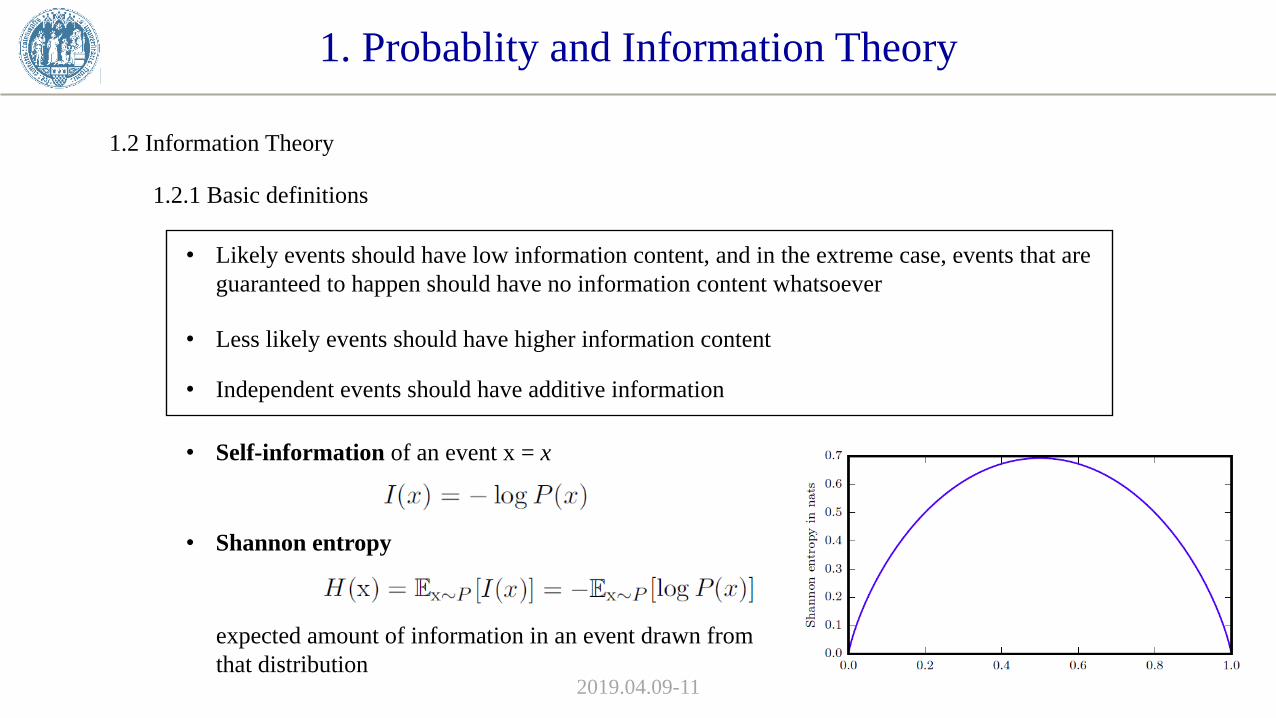
• Shannon entropy
expected amount of information in an event drawn from
that distribution
1. Probablity and Information Theory
1.2 Information Theory
1.2.1 Basic definitions
2019.04.09-11
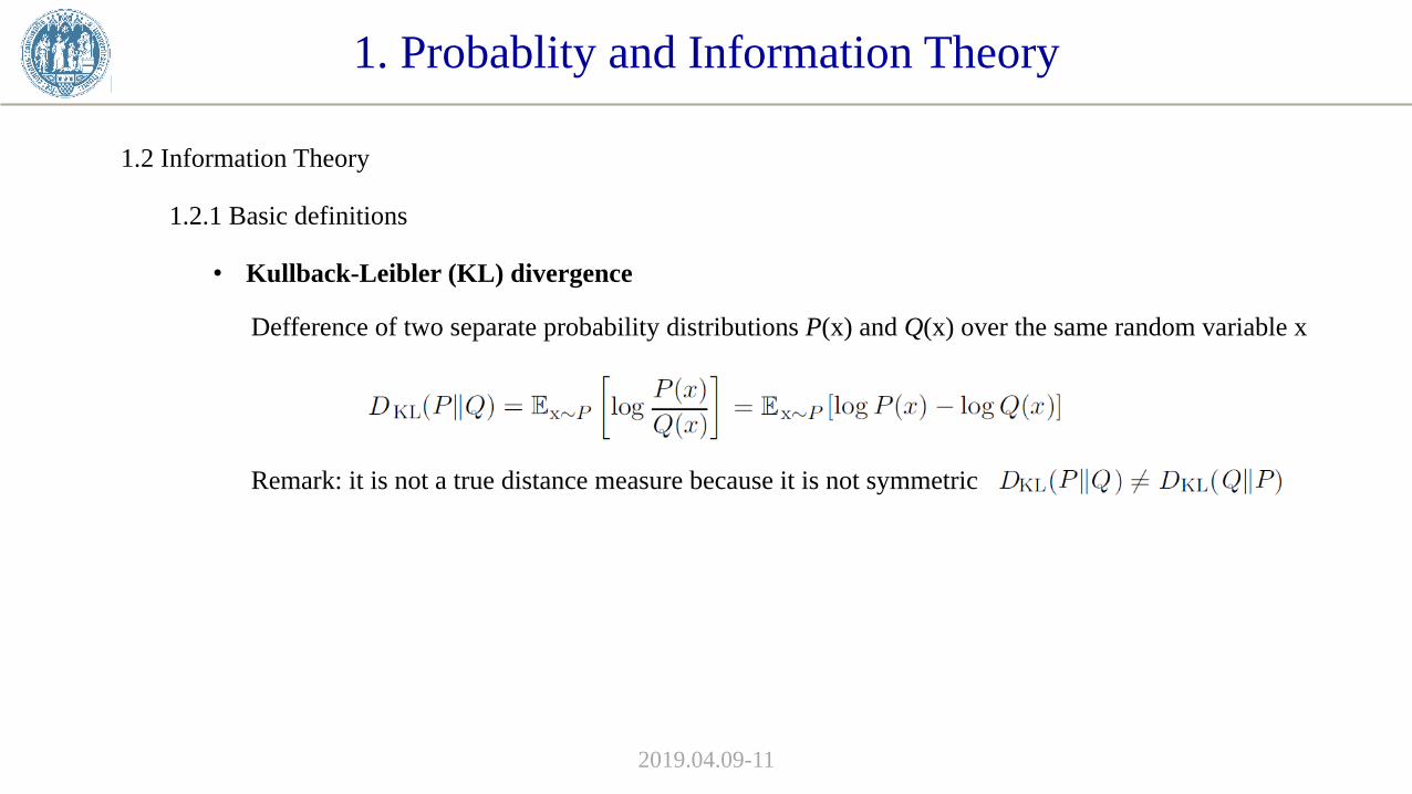
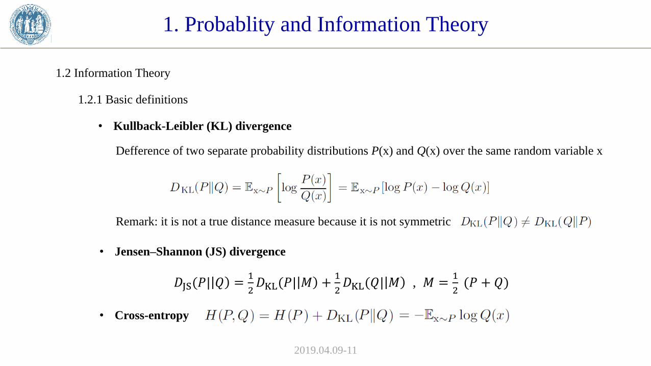
• Kullback-Leibler (KL) divergence
Defference of two separate probability distributions P(x) and Q(x) over the same random variable x
Remark: it is not a true distance measure because it is not symmetric

1. Probablity and Information Theory
1.2 Information Theory
1.2.1 Basic definitions
2019.04.09-11
• Kullback-Leibler (KL) divergence
Defference of two separate probability distributions P(x) and Q(x) over the same random variable x
Remark: it is not a true distance measure because it is not symmetric
• Jensen–Shannon (JS) divergence
• Cross-entropy
𝐷JS(𝑃| 𝑄 =1
2𝐷KL(𝑃| 𝑀 +
1
2𝐷KL(𝑄| 𝑀 , 𝑀 =
1
2(𝑃 + 𝑄)
1. Probablity and Information Theory
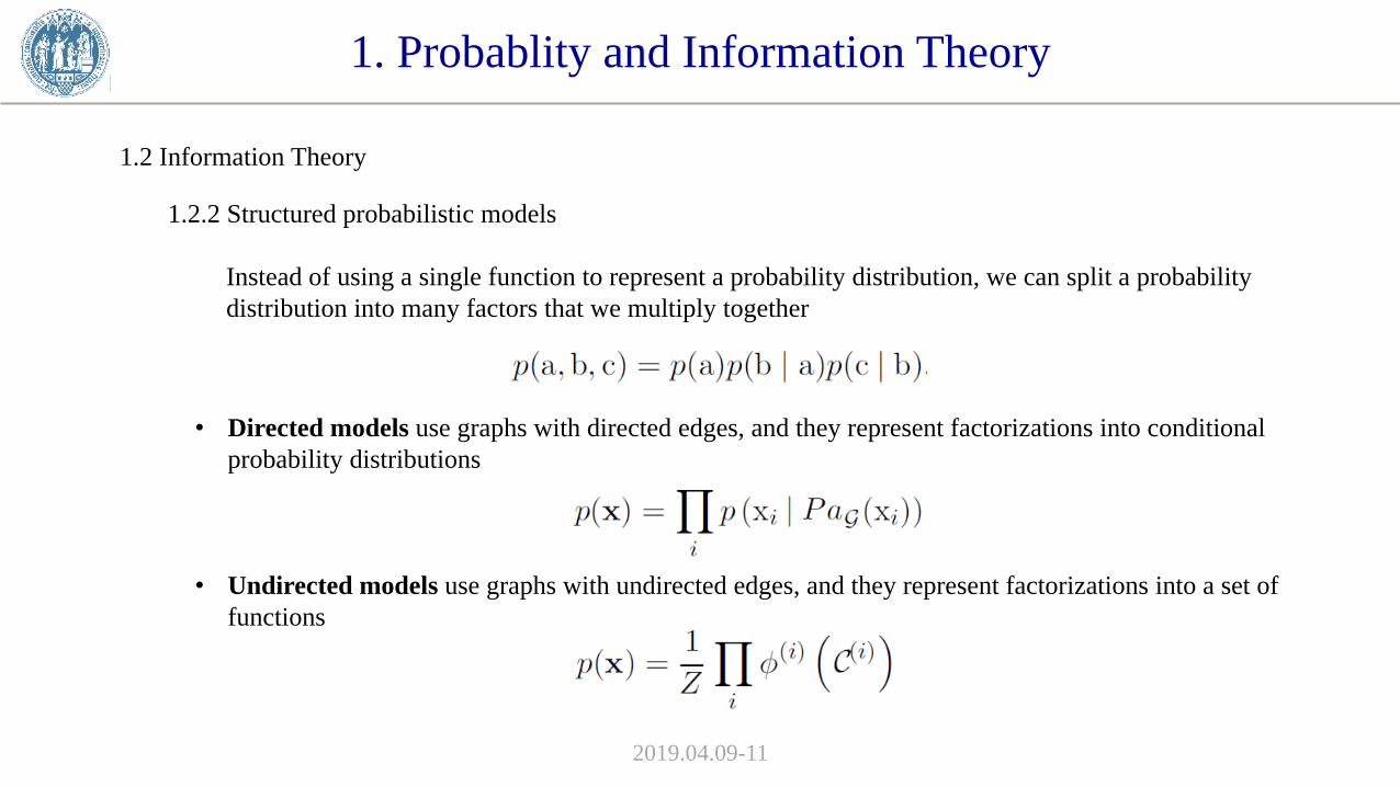
1.2 Information Theory
1.2.2 Structured probabilistic models
2019.04.09-11
Instead of using a single function to represent a probability distribution, we can split a probability
distribution into many factors that we multiply together
• Directed models use graphs with directed edges, and they represent factorizations into conditional
probability distributions
• Undirected models use graphs with undirected edges, and they represent factorizations into a set of
functions
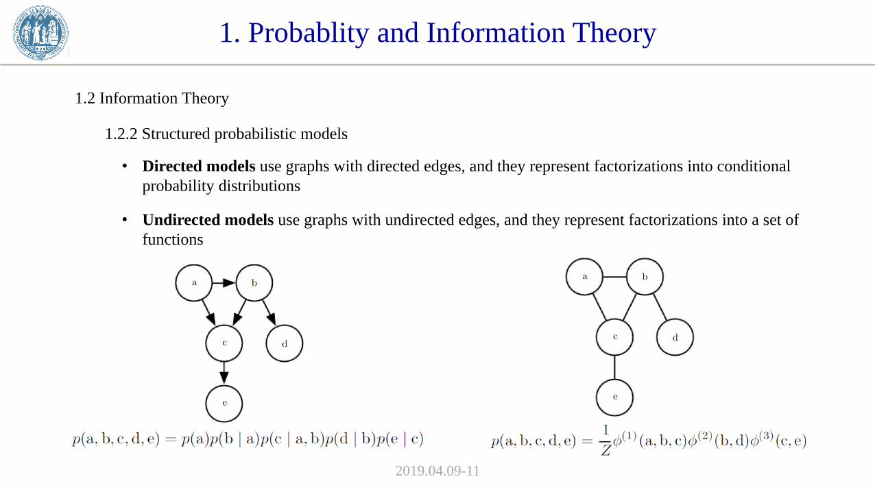
1. Probablity and Information Theory
1.2 Information Theory
1.2.2 Structured probabilistic models
2019.04.09-11
• Directed models use graphs with directed edges, and they represent factorizations into conditional
probability distributions
• Undirected models use graphs with undirected edges, and they represent factorizations into a set of
functions
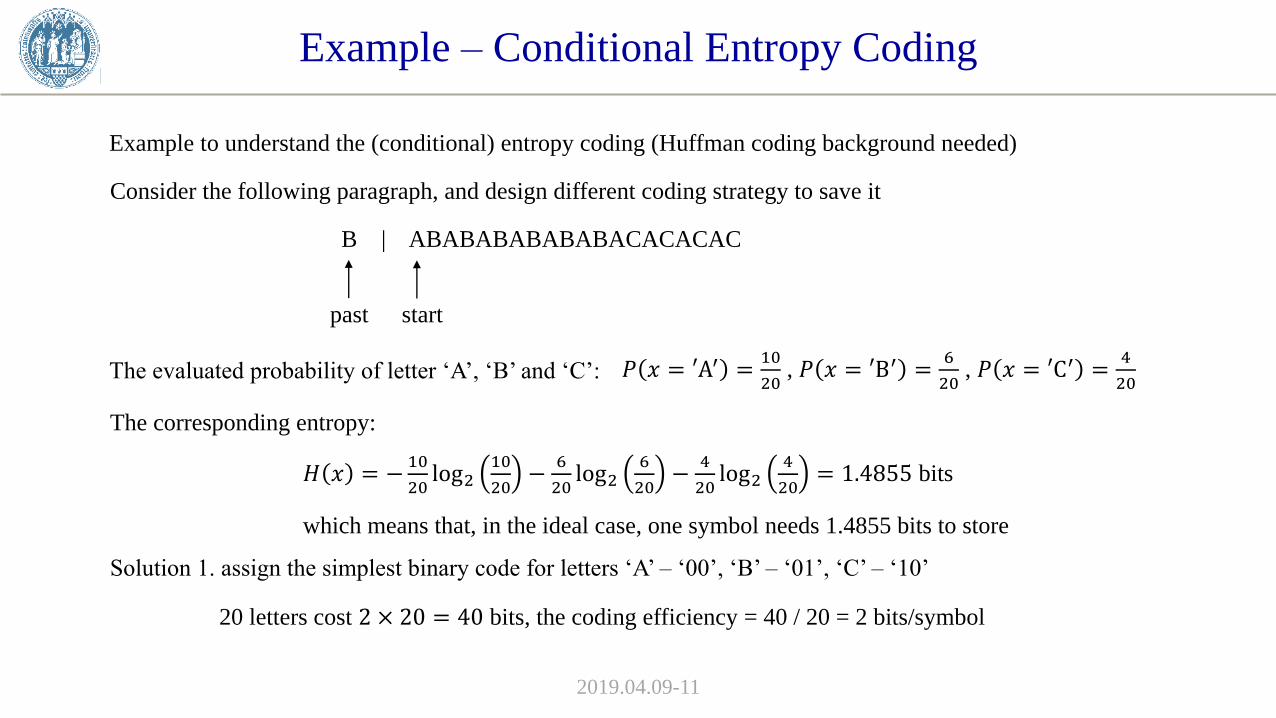
Example – Conditional Entropy Coding
Example to understand the (conditional) entropy coding (Huffman coding background needed)
Consider the following paragraph, and design different coding strategy to save it
2019.04.09-11
B | ABABABABABABACACACAC
past start
The evaluated probability of letter ‘A’, ‘B’ and ‘C’: 𝑃 𝑥 = ′A′ =10
20, 𝑃 𝑥 = ′B′ =
6
20, 𝑃 𝑥 = ′C′ =
4
20
The corresponding entropy:
𝐻 𝑥 = −10
20log2
10
20−
6
20log2
6
20−
4
20log2
4
20= 1.4855 bits
which means that, in the ideal case, one symbol needs 1.4855 bits to store
Solution 1. assign the simplest binary code for letters ‘A’ – ‘00’, ‘B’ – ‘01’, ‘C’ – ‘10’
20 letters cost 2 × 20 = 40 bits, the coding efficiency = 40 / 20 = 2 bits/symbol
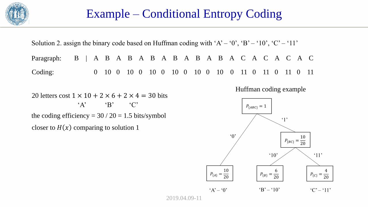
Example – Conditional Entropy Coding
2019.04.09-11
Paragraph:
Solution 2. assign the binary code based on Huffman coding with ‘A’ – ‘0’, ‘B’ – ‘10’, ‘C’ – ‘11’
20 letters cost 1 × 10 + 2 × 6 + 2 × 4 = 30 bits
Coding: 0 10 0 10 0 10 0 10 0 10 0 10 0 11 0 11 0 11 0 11
the coding efficiency = 30 / 20 = 1.5 bits/symbol
‘A’ ‘B’ ‘C’
closer to 𝐻 𝑥 comparing to solution 1
𝑃{𝐴} =10
20𝑃{𝐵} =
6
20𝑃{𝐶} =
4
20
𝑃{𝐵𝐶} =10
20
𝑃{𝐴𝐵𝐶} = 1
‘0’
‘1’
‘10’ ‘11’
‘A’ – ‘0’ ‘B’ – ‘10’ ‘C’ – ‘11’
Huffman coding example
B | A B A B A B A B A B A B A C A C A C A C

Example – Conditional Entropy Coding
2019.04.09-11
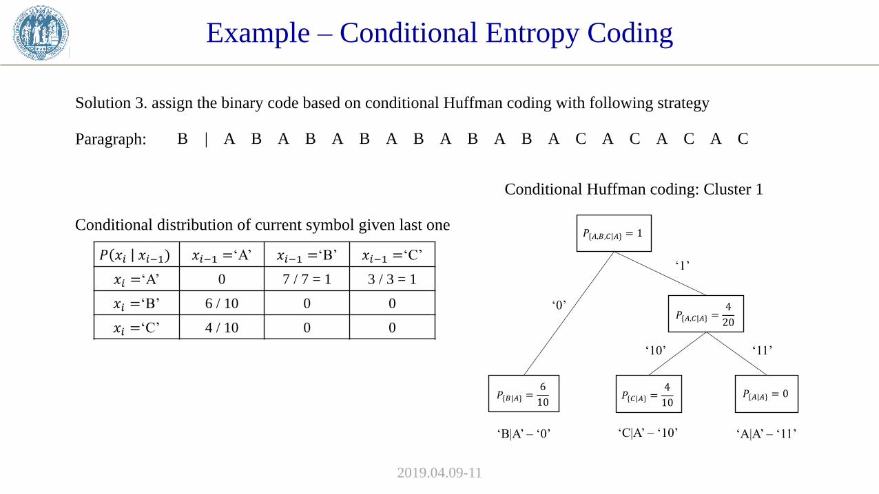
Solution 3. assign the binary code based on conditional Huffman coding with following strategy
Cluster 1: ‘A | A’ – ‘11’, ‘B | A’ – ‘0’, ‘C | A’ – ‘10’ symbol A, B, C conditioned by symbol A
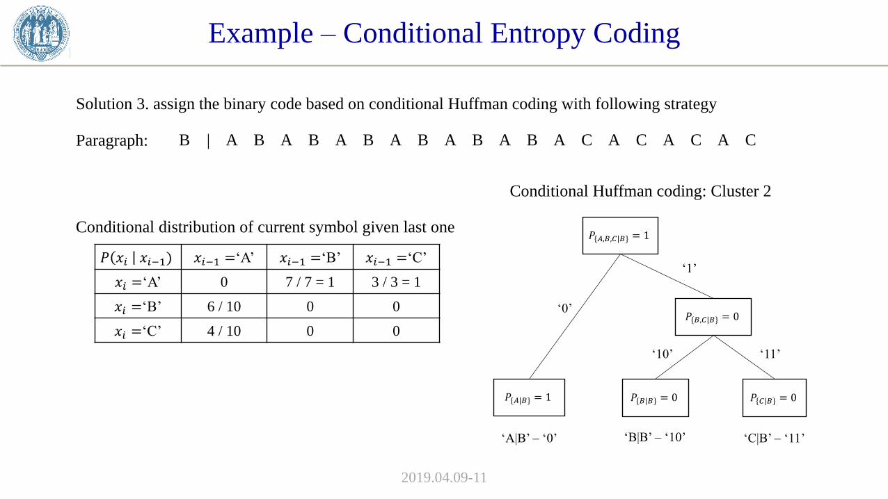
Cluster 2: ‘A | B’ – ‘0’, ‘B | B’ – ‘10’, ‘C | B’ – ‘11’ symbol A, B, C conditioned by symbol B
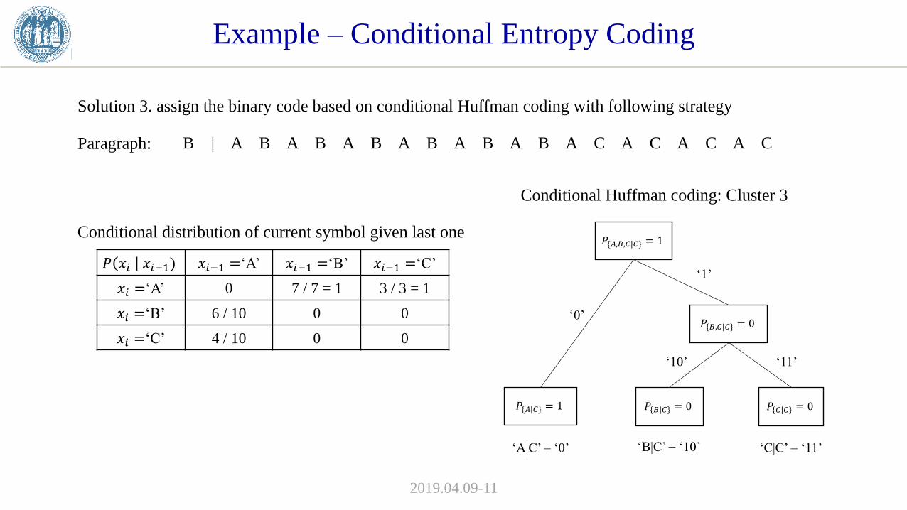
Cluster 3: ‘A | C’ – ‘0’, ‘B | C’ – ‘10’, ‘C | C’ – ‘11’ symbol A, B, C conditioned by symbol C
Paragraph:
past start
Case 1: from past ‘B’ to the first letter ‘A’, we have state ‘A’ conditioned by ‘B’, assign code ‘0’ based on cluster 2
Case 1: ‘0’ Case 2: ‘0’
Case 2: from past ‘A’ to the current ‘B’, we have state ‘B’ conditioned by ‘A’, assign code ‘0’ based on cluster 1
Case 3: ‘10’
Case 3: from past ‘A’ to the current ‘C’, we have state ‘C’ conditioned by ‘A’, assign code ‘10’ based on cluster 1
Paragraph:
Coding: 0 0 0 0 0 0 0 0 0 0 0 0 0 10 0 10 0 10 0 10
20 letters cost 24 bits. The coding efficiency = 24 / 20 = 1.2 bits/symbol, which is even less than 𝐻 𝑥 !!!
B | A B A B A B A B A B A B A C A C A C A C
B | A B A B A B A B A B A B A C A C A C A C
Example – Conditional Entropy Coding
2019.04.09-11
Solution 3. assign the binary code based on conditional Huffman coding with following strategy
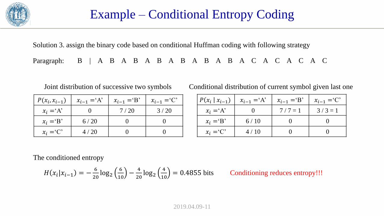
Paragraph: B | A B A B A B A B A B A B A C A C A C A C
𝑃(𝑥𝑖 , 𝑥𝑖−1) 𝑥𝑖−1 =‘A’ 𝑥𝑖−1 =‘B’ 𝑥𝑖−1 =‘C’
𝑥𝑖 =‘A’ 0 7 / 20 3 / 20
𝑥𝑖 =‘B’ 6 / 20 0 0
𝑥𝑖 =‘C’ 4 / 20 0 0
𝑃 𝑥𝑖 𝑥𝑖−1) 𝑥𝑖−1 =‘A’ 𝑥𝑖−1 =‘B’ 𝑥𝑖−1 =‘C’
𝑥𝑖 =‘A’ 0 7 / 7 = 1 3 / 3 = 1
𝑥𝑖 =‘B’ 6 / 10 0 0
𝑥𝑖 =‘C’ 4 / 10 0 0
Joint distribution of successive two symbols Conditional distribution of current symbol given last one
The conditioned entropy
𝐻 𝑥𝑖|𝑥𝑖−1 = −6
20log2
6
10−
4
20log2
4
10= 0.4855 bits Conditioning reduces entropy!!!
Example – Conditional Entropy Coding
2019.04.09-11
Solution 3. assign the binary code based on conditional Huffman coding with following strategy
Paragraph: B | A B A B A B A B A B A B A C A C A C A C
𝑃 𝑥𝑖 𝑥𝑖−1) 𝑥𝑖−1 =‘A’ 𝑥𝑖−1 =‘B’ 𝑥𝑖−1 =‘C’
𝑥𝑖 =‘A’ 0 7 / 7 = 1 3 / 3 = 1
𝑥𝑖 =‘B’ 6 / 10 0 0
𝑥𝑖 =‘C’ 4 / 10 0 0
Conditional distribution of current symbol given last one
𝑃{𝐵|𝐴} =6
10𝑃{𝐶|𝐴} =
4
10𝑃{𝐴|𝐴} = 0
𝑃{𝐴,𝐶|𝐴} =4
20
𝑃{𝐴,𝐵,𝐶|𝐴} = 1
‘0’
‘1’
‘10’ ‘11’
‘B|A’ – ‘0’ ‘C|A’ – ‘10’ ‘A|A’ – ‘11’
Conditional Huffman coding: Cluster 1
Example – Conditional Entropy Coding
2019.04.09-11
Solution 3. assign the binary code based on conditional Huffman coding with following strategy
Paragraph: B | A B A B A B A B A B A B A C A C A C A C
𝑃 𝑥𝑖 𝑥𝑖−1) 𝑥𝑖−1 =‘A’ 𝑥𝑖−1 =‘B’ 𝑥𝑖−1 =‘C’
𝑥𝑖 =‘A’ 0 7 / 7 = 1 3 / 3 = 1
𝑥𝑖 =‘B’ 6 / 10 0 0
𝑥𝑖 =‘C’ 4 / 10 0 0
Conditional distribution of current symbol given last one
𝑃{𝐴|𝐵} = 1 𝑃{𝐵|𝐵} = 0 𝑃{𝐶|𝐵} = 0
𝑃{𝐵,𝐶|𝐵} = 0
𝑃{𝐴,𝐵,𝐶|𝐵} = 1
‘0’
‘1’
‘10’ ‘11’
‘A|B’ – ‘0’ ‘B|B’ – ‘10’ ‘C|B’ – ‘11’
Conditional Huffman coding: Cluster 2
Example – Conditional Entropy Coding
2019.04.09-11
Solution 3. assign the binary code based on conditional Huffman coding with following strategy
Paragraph: B | A B A B A B A B A B A B A C A C A C A C
𝑃 𝑥𝑖 𝑥𝑖−1) 𝑥𝑖−1 =‘A’ 𝑥𝑖−1 =‘B’ 𝑥𝑖−1 =‘C’
𝑥𝑖 =‘A’ 0 7 / 7 = 1 3 / 3 = 1
𝑥𝑖 =‘B’ 6 / 10 0 0
𝑥𝑖 =‘C’ 4 / 10 0 0
Conditional distribution of current symbol given last one
𝑃{𝐴|𝐶} = 1 𝑃{𝐵|𝐶} = 0 𝑃{𝐶|𝐶} = 0
𝑃{𝐵,𝐶|𝐶} = 0
𝑃{𝐴,𝐵,𝐶|𝐶} = 1
‘0’
‘1’
‘10’ ‘11’
‘A|C’ – ‘0’ ‘B|C’ – ‘10’ ‘C|C’ – ‘11’
Conditional Huffman coding: Cluster 3