Embed Size (px)
Citation preview
MATHEMATICAL INSTITUTE
UNIVERSITY OF OXFORD
Computational Mathematics
Student GuideMichaelmas Term 2021
by
Prof. Nick Trefethen
ii
Acknowledgments: This course guide is adapted from previous versions by Andrew Thompson,Alberto Paganini, Estelle Massart, Vidit Nanda, and others before them. We are grateful to all previousauthors.
©2021 Mathematical Institute, University of Oxford
iii
Notes for the 2021/2022 Course
The course will be in two parts: Part I in Michaelmas Term Weeks 3–8 and Hilary Term Weeks 1–2,and Part II in Hilary Term Weeks 3–8. For Part I, you will attend scheduled practical sessions everyfortnight starting in Week 3 Michaelmas Term. The practical sessions are held in the MathematicalInstitute, Radcliffe Observatory Quarter.
Each practical session will be run by a demonstrator and may include a short lecture. You willneed to bring your laptop to these sessions. Please follow the instructions on the MathematicalInstitute website
https://www.maths.ox.ac.uk/members/it/software-personal-machines/matlab
to install MATLAB on your machine before the first session. Note that there are around 50 toolboxesavailable for download, and the only one you will require is the Symbolic Math Toolbox. The defaultsetting is to download all available toolboxes, which may take many hours using a standard broad-band connection. To avoid this, you can select just the Symbolic Math Toolbox (i.e., deselect all othertoolboxes) in the “Product Selection Window” stage of the installation process.
As an alternative to MATLAB, and in particular if you are a proficient computer user, you couldtry to use Octave (http://www.octave.org) which uses a very similar command syntax and is oftenregarded as a MATLAB clone. See Section 1.1.2.
Inevitably Prof. Trefethen will be unable to resist saying a few words now and then about Chebfun,the continuous analogue of MATLAB. If you are curious, see www.chebfun.org.
Time-line There are four problem sheets, which will be the focus of four corresponding demonstra-tor sessions, scheduled in weeks 3-4, 5-6, 7-8 of MT and 1-2 of HT, and which correspond to the fourchapters of the course.
Weeks Chapter3–4 MT 15–6 MT 27–8 MT 31–2 HT 4
Michaelmas term will place many demands on your time, but you need to put in the effort to ensurethat you make steady progress and finish Part I of the course by the end of Week 2, Hilary Term.
Assessment During Part I of the course, you may work collaboratively with others and—as always—you are encouraged to discuss mathematics and your studies with your peers. Your demonstrator willask you to submit work related to these sessions: chapter 1/2/3 exercises to be turned in at sessions2/3/4. However, none of the work in Part I will be formally assessed. Instead the material will act asa foundation enabling you to work individually during Part II. This individual work will be assessedand will count towards your Preliminary Examination as described in Examination Decrees & Regula-tions, 2021 and the current Course Handbook. (See your college tutor if you have any questions aboutthis aspect of the course.)
Course director The course director is Prof. Nick Trefethen. The demonstrators will be able to an-swer most questions; alternatively Prof. Trefethen can be contacted at [email protected].
Course website This manual and any extra course material (such as lecture notes) can be found onthe course website:
https://courses.maths.ox.ac.uk/course/view.php?id=44
Errata list If errors are found in this manual, they will be corrected and listed on the website above.It would be a good idea to check occasionally, especially if you think you’ve found an error.

iv
Contents
1 Introduction to MATLAB 11.1 What is MATLAB? . . . . . . . . . . . . . . . . . . . . . . . . . . . . . . . . . . . . . . . . 1
1.1.1 What is the Symbolic Math Toolbox? . . . . . . . . . . . . . . . . . . . . . . . . . . 11.1.2 What is Octave? . . . . . . . . . . . . . . . . . . . . . . . . . . . . . . . . . . . . . . 11.1.3 Learning MATLAB . . . . . . . . . . . . . . . . . . . . . . . . . . . . . . . . . . . . 2
1.2 The command prompt, variables, getting help . . . . . . . . . . . . . . . . . . . . . . . . 21.2.1 Using MATLAB’s built-in help system . . . . . . . . . . . . . . . . . . . . . . . . . 21.2.2 Assigning to variables . . . . . . . . . . . . . . . . . . . . . . . . . . . . . . . . . . 21.2.3 Floating-point numbers . . . . . . . . . . . . . . . . . . . . . . . . . . . . . . . . . 31.2.4 Symbolic computing . . . . . . . . . . . . . . . . . . . . . . . . . . . . . . . . . . . 41.2.5 Saving your work in .m file scripts . . . . . . . . . . . . . . . . . . . . . . . . . . . 51.2.6 Using symbols instead of numbers . . . . . . . . . . . . . . . . . . . . . . . . . . . 51.2.7 Built-in functions and help . . . . . . . . . . . . . . . . . . . . . . . . . . . . . . . 8
1.3 2D graphics . . . . . . . . . . . . . . . . . . . . . . . . . . . . . . . . . . . . . . . . . . . . 91.3.1 Simple line graphs . . . . . . . . . . . . . . . . . . . . . . . . . . . . . . . . . . . . 91.3.2 Parametric and polar plots . . . . . . . . . . . . . . . . . . . . . . . . . . . . . . . 10
2 Algebraic equations and calculus 122.1 Evaluating expressions . . . . . . . . . . . . . . . . . . . . . . . . . . . . . . . . . . . . . . 122.2 The solve command . . . . . . . . . . . . . . . . . . . . . . . . . . . . . . . . . . . . . . . 13
2.2.1 Solving equations symbolically . . . . . . . . . . . . . . . . . . . . . . . . . . . . . 132.2.2 Assumptions . . . . . . . . . . . . . . . . . . . . . . . . . . . . . . . . . . . . . . . 142.2.3 Solving equations numerically . . . . . . . . . . . . . . . . . . . . . . . . . . . . . 15
2.3 Differentiation and the diff command . . . . . . . . . . . . . . . . . . . . . . . . . . . . . 172.3.1 Differentiation of unknown functions . . . . . . . . . . . . . . . . . . . . . . . . . 19
2.4 Evaluating limits . . . . . . . . . . . . . . . . . . . . . . . . . . . . . . . . . . . . . . . . . 202.5 Integration . . . . . . . . . . . . . . . . . . . . . . . . . . . . . . . . . . . . . . . . . . . . . 21
2.5.1 The int operator . . . . . . . . . . . . . . . . . . . . . . . . . . . . . . . . . . . . . 212.5.2 Quadrature: numerical evaluation of integrals . . . . . . . . . . . . . . . . . . . . 22
3 Differential equations, sums, matrices and vectors 243.1 Solving ordinary differential equations using dsolve . . . . . . . . . . . . . . . . . . . . 243.2 Vectors and lists in MATLAB . . . . . . . . . . . . . . . . . . . . . . . . . . . . . . . . . . 26
3.2.1 Symbolic lists . . . . . . . . . . . . . . . . . . . . . . . . . . . . . . . . . . . . . . . 263.2.2 Indexing in lists . . . . . . . . . . . . . . . . . . . . . . . . . . . . . . . . . . . . . . 273.2.3 Vector operations . . . . . . . . . . . . . . . . . . . . . . . . . . . . . . . . . . . . . 27
3.3 Sets . . . . . . . . . . . . . . . . . . . . . . . . . . . . . . . . . . . . . . . . . . . . . . . . . 283.4 Sums and products . . . . . . . . . . . . . . . . . . . . . . . . . . . . . . . . . . . . . . . . 28
3.4.1 Simple “numerical” sums . . . . . . . . . . . . . . . . . . . . . . . . . . . . . . . . 283.4.2 Products . . . . . . . . . . . . . . . . . . . . . . . . . . . . . . . . . . . . . . . . . . 293.4.3 Symbolic manipulation of sums and products . . . . . . . . . . . . . . . . . . . . 29
3.5 Arrays, matrices and vectors . . . . . . . . . . . . . . . . . . . . . . . . . . . . . . . . . . . 313.5.1 Matrix definition . . . . . . . . . . . . . . . . . . . . . . . . . . . . . . . . . . . . . 313.5.2 Rows, columns and submatrices . . . . . . . . . . . . . . . . . . . . . . . . . . . . 31
v
CONTENTS vi
3.5.3 Operators on matrices and vectors . . . . . . . . . . . . . . . . . . . . . . . . . . . 323.5.4 Simultaneous equations . . . . . . . . . . . . . . . . . . . . . . . . . . . . . . . . . 333.5.5 Eigenvalues and eigenvectors . . . . . . . . . . . . . . . . . . . . . . . . . . . . . . 33
3.6 Meshgrids and 3D plots . . . . . . . . . . . . . . . . . . . . . . . . . . . . . . . . . . . . . 333.6.1 Logical masks . . . . . . . . . . . . . . . . . . . . . . . . . . . . . . . . . . . . . . . 333.6.2 Meshgrid . . . . . . . . . . . . . . . . . . . . . . . . . . . . . . . . . . . . . . . . . 343.6.3 3D plotting . . . . . . . . . . . . . . . . . . . . . . . . . . . . . . . . . . . . . . . . 34
4 Loops, conditionals and functions 364.1 Loops . . . . . . . . . . . . . . . . . . . . . . . . . . . . . . . . . . . . . . . . . . . . . . . . 36
4.1.1 Approximate solutions to equations . . . . . . . . . . . . . . . . . . . . . . . . . . 374.2 Conditionals . . . . . . . . . . . . . . . . . . . . . . . . . . . . . . . . . . . . . . . . . . . . 384.3 Functions . . . . . . . . . . . . . . . . . . . . . . . . . . . . . . . . . . . . . . . . . . . . . . 394.4 Examples of functions . . . . . . . . . . . . . . . . . . . . . . . . . . . . . . . . . . . . . . 40
4.4.1 Finding the arithmetic mean of a set of numbers . . . . . . . . . . . . . . . . . . . 404.4.2 Taylor’s theorem . . . . . . . . . . . . . . . . . . . . . . . . . . . . . . . . . . . . . 414.4.3 Euler’s method . . . . . . . . . . . . . . . . . . . . . . . . . . . . . . . . . . . . . . 414.4.4 Euclid’s algorithm . . . . . . . . . . . . . . . . . . . . . . . . . . . . . . . . . . . . 424.4.5 A simple matrix function . . . . . . . . . . . . . . . . . . . . . . . . . . . . . . . . 43
4.5 Debugging . . . . . . . . . . . . . . . . . . . . . . . . . . . . . . . . . . . . . . . . . . . . . 434.6 Further exercise . . . . . . . . . . . . . . . . . . . . . . . . . . . . . . . . . . . . . . . . . . 44
A Simplification 45A.1 Expand . . . . . . . . . . . . . . . . . . . . . . . . . . . . . . . . . . . . . . . . . . . . . . . 45A.2 Factor . . . . . . . . . . . . . . . . . . . . . . . . . . . . . . . . . . . . . . . . . . . . . . . . 46A.3 Collect . . . . . . . . . . . . . . . . . . . . . . . . . . . . . . . . . . . . . . . . . . . . . . . 46A.4 Simplify . . . . . . . . . . . . . . . . . . . . . . . . . . . . . . . . . . . . . . . . . . . . . . 46
B Other advanced topics 48B.1 MATLAB “handle” functions and anonymous functions . . . . . . . . . . . . . . . . . . 48B.2 Variable precision arithmetic . . . . . . . . . . . . . . . . . . . . . . . . . . . . . . . . . . . 48B.3 Cell Arrays . . . . . . . . . . . . . . . . . . . . . . . . . . . . . . . . . . . . . . . . . . . . . 49
Chapter 1
Introduction to MATLAB
In this chapter you will learn about:
• Accessing MATLAB,
• using MATLAB as a calculator,
• MATLAB identifiers, constants and functions,
• using the MATLAB help system,
• making .m file scripts,
• plotting simple line graphs.
1.1 What is MATLAB?
MATLAB is often described as a problem solving environment. It is a programming language and aset of tools for solving mathematical problems.
The name MATLAB was originally a contraction of “Matrix Laboratory” and indeed MATLAB’score strength is numerical computing involving matrices, vectors and linear algebra. It also has exten-sive plotting and graphics routines.
1.1.1 What is the Symbolic Math Toolbox?
The Symbolic Math Toolbox is an add-on for MATLAB which adds symbolic as opposed to numericalcomputing abilities. The strength of such a system is the ability to manipulate algebraic expressions.The Symbolic Math Toolbox can be used to solve algebraic equations, factorize polynomials and sim-plify rational expressions. It can also solve some differential equations. It can perform many of thestandard operations of analysis such as evaluating sums, limits, derivatives and integrals. Under thehood, the Symbolic Math Toolbox is powered by a computer algebra system called MuPAD.
The combination of MATLAB and the Symbolic Math Toolbox allows the user to mix symbolic andnumerical computing within the MATLAB environment.
1.1.2 What is Octave?
Some people are concerned about issues surrounding computing. Should software be freely available?If these matters are important to you, you might want to consider Octave (http://www.octave.org)as an alternative to MATLAB. It is Free Software (also known as Open Source Software) which meansyou can use it without restriction, study its source code, improve it, and share it with others as youwish. None of these things are true of MATLAB.
OctSymPy (see http://github.com/cbm755/octsympy) is an add-on package that adds symboliccomputing features to Octave (it is analogous to the Symbolic Math Toolbox for MATLAB). OctSymPyis new software developed right here at Oxford!
1
CHAPTER 1. INTRODUCTION TO MATLAB 2
The syntax of commands in Octave is almost the same as in MATLAB, and the differences are welldocumented. But having said that, this manual will concentrate on MATLAB and this is likely the toolyour demonstrators will know best. Try Octave if you wish, but do so “at your own risk”.
1.1.3 Learning MATLAB
In order to become technically adept at using MATLAB it is important that you attempt all the exer-cises contained in this manual; as with most tools, MATLAB is best learned by actually using it to domathematics, and this should be practised as often as possible. Try to incorporate MATLAB into yourweekly problem sheets, by using it to check some of your hand-written answers. Examples includesubstituting your solution back into the equation and plotting an answer to make sure it makes sense.
In the rest of this chapter, we will give a brief introduction to MATLAB, outlining some of its basicfeatures and illustrating them with some short examples. The output of each command line is notprinted in this manual; after executing each line you should check that the output is as you wouldexpect. If it is not, then you should think about why this might be, and if necessary consult yourdemonstrator.
1.2 The command prompt, variables, getting help
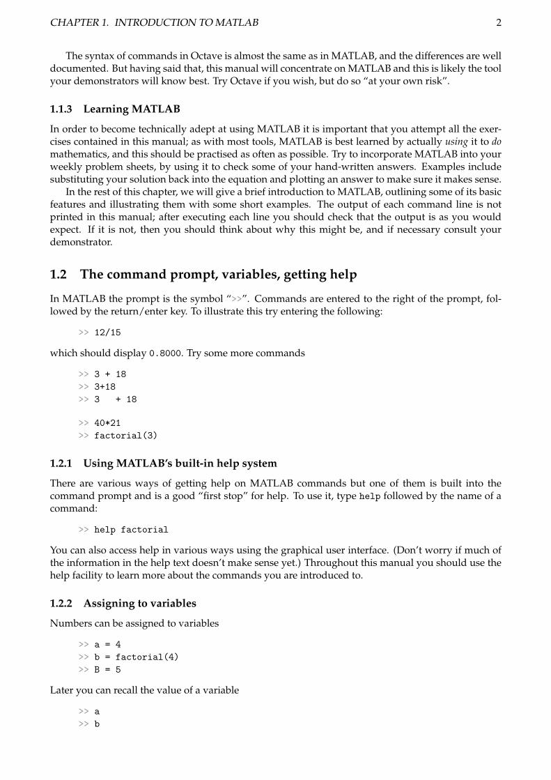
In MATLAB the prompt is the symbol “>>”. Commands are entered to the right of the prompt, fol-lowed by the return/enter key. To illustrate this try entering the following:
>> 12/15
which should display 0.8000. Try some more commands
>> 3 + 18
>> 3+18
>> 3 + 18
>> 40*21
>> factorial(3)
1.2.1 Using MATLAB’s built-in help system
There are various ways of getting help on MATLAB commands but one of them is built into thecommand prompt and is a good “first stop” for help. To use it, type help followed by the name of acommand:
>> help factorial
You can also access help in various ways using the graphical user interface. (Don’t worry if much ofthe information in the help text doesn’t make sense yet.) Throughout this manual you should use thehelp facility to learn more about the commands you are introduced to.
1.2.2 Assigning to variables
Numbers can be assigned to variables
>> a = 4
>> b = factorial(4)
>> B = 5
Later you can recall the value of a variable
>> a
>> b
CHAPTER 1. INTRODUCTION TO MATLAB 3
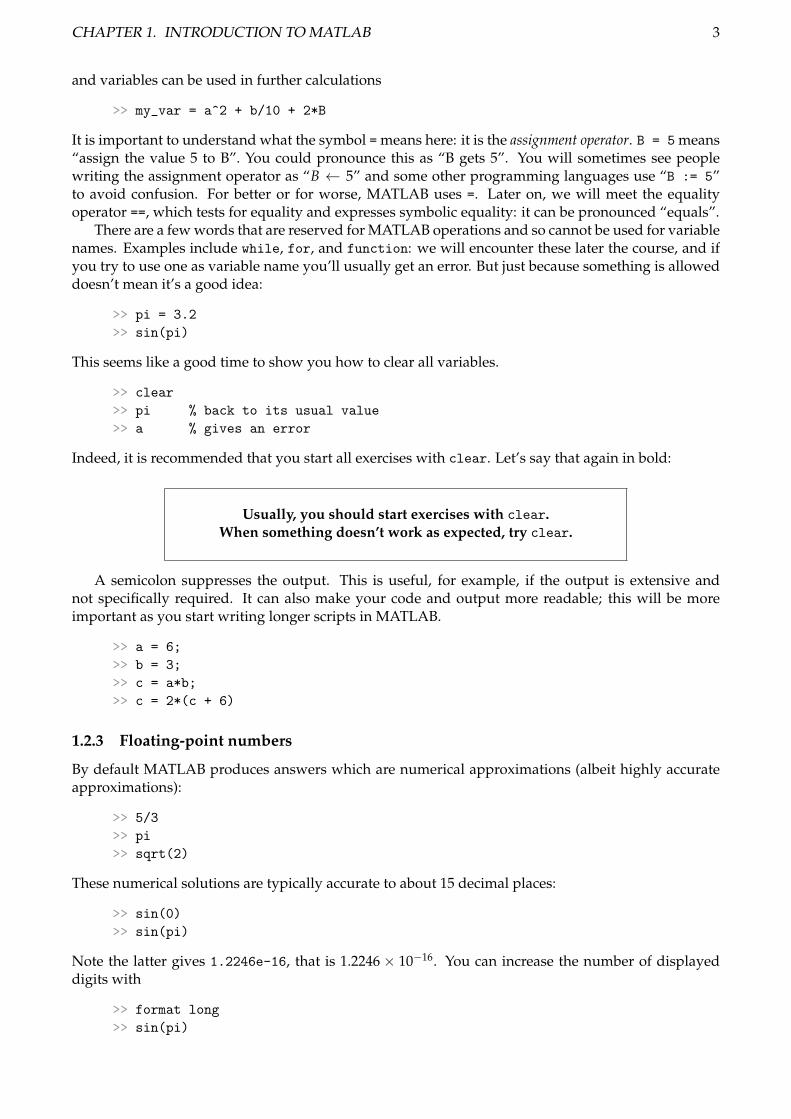
and variables can be used in further calculations
>> my_var = a^2 + b/10 + 2*B
It is important to understand what the symbol = means here: it is the assignment operator. B = 5 means“assign the value 5 to B”. You could pronounce this as “B gets 5”. You will sometimes see peoplewriting the assignment operator as “B ← 5” and some other programming languages use “B := 5”to avoid confusion. For better or for worse, MATLAB uses =. Later on, we will meet the equalityoperator ==, which tests for equality and expresses symbolic equality: it can be pronounced “equals”.
There are a few words that are reserved for MATLAB operations and so cannot be used for variablenames. Examples include while, for, and function: we will encounter these later the course, and ifyou try to use one as variable name you’ll usually get an error. But just because something is alloweddoesn’t mean it’s a good idea:
>> pi = 3.2
>> sin(pi)
This seems like a good time to show you how to clear all variables.
>> clear
>> pi % back to its usual value
>> a % gives an error
Indeed, it is recommended that you start all exercises with clear. Let’s say that again in bold:
Usually, you should start exercises with clear.When something doesn’t work as expected, try clear.
A semicolon suppresses the output. This is useful, for example, if the output is extensive andnot specifically required. It can also make your code and output more readable; this will be moreimportant as you start writing longer scripts in MATLAB.
>> a = 6;
>> b = 3;
>> c = a*b;
>> c = 2*(c + 6)
1.2.3 Floating-point numbers
By default MATLAB produces answers which are numerical approximations (albeit highly accurateapproximations):
>> 5/3
>> pi
>> sqrt(2)
These numerical solutions are typically accurate to about 15 decimal places:
>> sin(0)
>> sin(pi)
Note the latter gives 1.2246e-16, that is 1.2246× 10⁻¹⁶. You can increase the number of displayeddigits with
>> format long
>> sin(pi)
CHAPTER 1. INTRODUCTION TO MATLAB 4
but note this has no effect on the actual accuracy of the expression, just its display.Internally, MATLAB by default stores numbers in “IEEE Double-Precision Floating Point Arith-
metic” or just double for short. Each double takes 8 bytes (that is 64 bits, “binary digits”) in thememory of the computer. The 64 bits is used to store numbers in scientific notation with a certainnumber of bits for the exponent (the “-16” in our example above) and the rest for the coefficient (1.222in our example).
Computers are very fast at doing arithmetic on doubles, and this forms the basis for much of com-putation. For example, encoding/decoding your voice, music, and video on your phone, performinglarge-scale climate simulations, finding a location from GPS satellites, or finding eigenvalues of largematrices all involve billions of operators on doubles (or on similar structures of lower precision). Asurprising number of things we do (e.g., searching the internet) are related to the linear algebra prob-lem of “finding eigenvalues of large matrices”.
However, sometimes it’s nice when 6/9 becomes 2/3, not “0.666666666666667”. Particularly whenlearning or studying mathematics, we are often less interested in the numerical solution of somethingbut rather in the how and why of it. Think about the area under a curve (a number, rather easilyapproximated) versus the indefinite integral (a general expression). We want the computer to do boththese tasks.
1.2.4 Symbolic computing
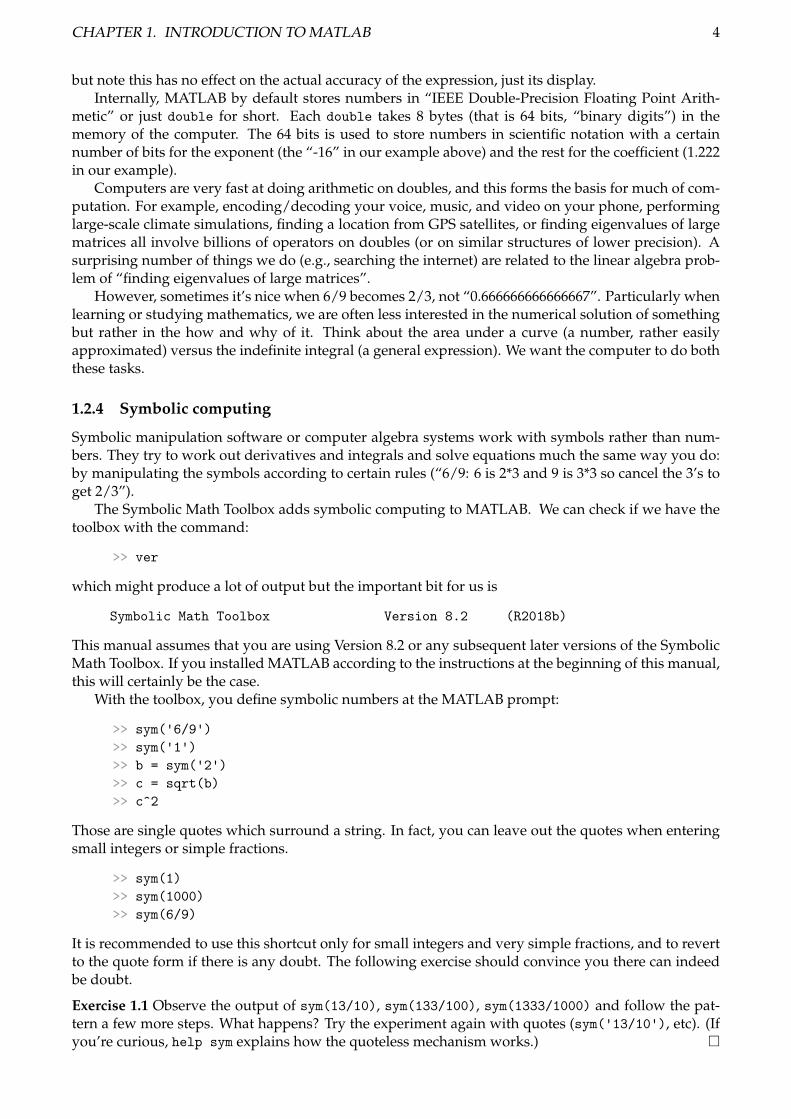
Symbolic manipulation software or computer algebra systems work with symbols rather than num-bers. They try to work out derivatives and integrals and solve equations much the same way you do:by manipulating the symbols according to certain rules (“6/9: 6 is 2*3 and 9 is 3*3 so cancel the 3’s toget 2/3”).
The Symbolic Math Toolbox adds symbolic computing to MATLAB. We can check if we have thetoolbox with the command:
>> ver
which might produce a lot of output but the important bit for us is
Symbolic Math Toolbox Version 8.2 (R2018b)
This manual assumes that you are using Version 8.2 or any subsequent later versions of the SymbolicMath Toolbox. If you installed MATLAB according to the instructions at the beginning of this manual,this will certainly be the case.
With the toolbox, you define symbolic numbers at the MATLAB prompt:
>> sym('6/9')
>> sym('1')
>> b = sym('2')
>> c = sqrt(b)
>> c^2
Those are single quotes which surround a string. In fact, you can leave out the quotes when enteringsmall integers or simple fractions.
>> sym(1)
>> sym(1000)
>> sym(6/9)
It is recommended to use this shortcut only for small integers and very simple fractions, and to revertto the quote form if there is any doubt. The following exercise should convince you there can indeedbe doubt.
Exercise 1.1 Observe the output of sym(13/10), sym(133/100), sym(1333/1000) and follow the pat-tern a few more steps. What happens? Try the experiment again with quotes (sym('13/10'), etc). (Ifyou’re curious, help sym explains how the quoteless mechanism works.) �
CHAPTER 1. INTRODUCTION TO MATLAB 5
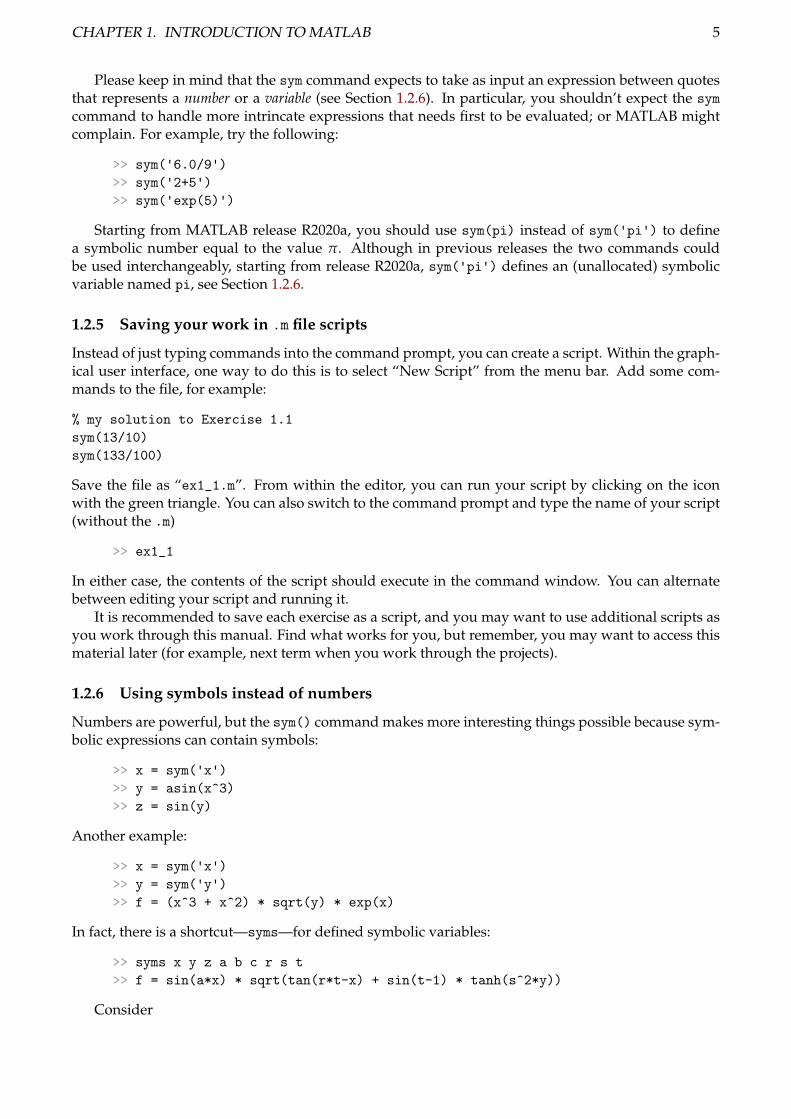
Please keep in mind that the sym command expects to take as input an expression between quotesthat represents a number or a variable (see Section 1.2.6). In particular, you shouldn’t expect the sym
command to handle more intrincate expressions that needs first to be evaluated; or MATLAB mightcomplain. For example, try the following:
>> sym('6.0/9')
>> sym('2+5')
>> sym('exp(5)')
Starting from MATLAB release R2020a, you should use sym(pi) instead of sym('pi') to definea symbolic number equal to the value π. Although in previous releases the two commands couldbe used interchangeably, starting from release R2020a, sym('pi') defines an (unallocated) symbolicvariable named pi, see Section 1.2.6.
1.2.5 Saving your work in .m file scripts
Instead of just typing commands into the command prompt, you can create a script. Within the graph-ical user interface, one way to do this is to select “New Script” from the menu bar. Add some com-mands to the file, for example:
% my solution to Exercise 1.1
sym(13/10)
sym(133/100)
Save the file as “ex1_1.m”. From within the editor, you can run your script by clicking on the iconwith the green triangle. You can also switch to the command prompt and type the name of your script(without the .m)
>> ex1_1
In either case, the contents of the script should execute in the command window. You can alternatebetween editing your script and running it.
It is recommended to save each exercise as a script, and you may want to use additional scripts asyou work through this manual. Find what works for you, but remember, you may want to access thismaterial later (for example, next term when you work through the projects).
1.2.6 Using symbols instead of numbers
Numbers are powerful, but the sym() command makes more interesting things possible because sym-bolic expressions can contain symbols:
>> x = sym('x')
>> y = asin(x^3)
>> z = sin(y)
Another example:
>> x = sym('x')
>> y = sym('y')
>> f = (x^3 + x^2) * sqrt(y) * exp(x)
In fact, there is a shortcut—syms—for defined symbolic variables:
>> syms x y z a b c r s t
>> f = sin(a*x) * sqrt(tan(r*t-x) + sin(t-1) * tanh(s^2*y))
Consider
CHAPTER 1. INTRODUCTION TO MATLAB 6
>> a = sym(6)
>> b = sym(2)*a
>> c = sym('2*a')
What happened? The result in b is correct, but c throws an error. As mentioned in the end of Section1.2.4, this is because MATLAB does not allow you to write expressions inside quotes and pass themto sym. For example, instead of f = sym('a * x + b'), you should write
>> syms a x b
>> f = a*x + b
If you really need to pass a string instead of a number or a variable to sym, you can use the commandstr2sym. For example, you can write
>> str2sym('sqrt(2)')
However, passing expressions as strings may not always produce the desired result. For instance,compare the outputs of the following commands.
>> a = sym(6)
>> b = sym(2)*a
>> c = str2sym('2*a')
In Section 2.1, we will learn about the subs command, which will help push assigned variablesinto expressions.
Variable types and casting
We have encountered two types (“classes”) of objects so far: doubles, which store numbers with afinite precision, and syms, which store symbolic expressions. It will often be important to keep trackof which is which. The whos command can help.
>> clear
>> a = sym('6/9')
>> b = 6/9
>> whos
Now we can ask some useful questions about what happens when you combine objects.
Exercise 1.2 Use MATLAB to evaluate the following:
>> a = sym(2/3)
>> b = 5/3
>> c = a + b
>> d = b*a
>> e = a^b
>> f = (2/3) ^ (sym(5/3))
>> e - f
>> whos
From these results, what does MATLAB typically do when it performs a binary operation which com-bines a double and a sym? This is known as casting. �
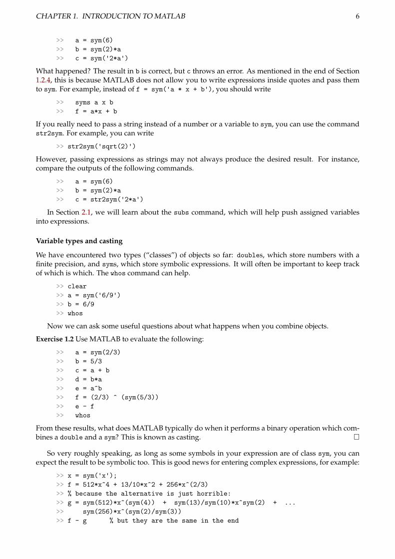
So very roughly speaking, as long as some symbols in your expression are of class sym, you canexpect the result to be symbolic too. This is good news for entering complex expressions, for example:
>> x = sym('x');
>> f = 512*x^4 + 13/10*x^2 + 256*x^(2/3)
>> % because the alternative is just horrible:
>> g = sym(512)*x^(sym(4)) + sym(13)/sym(10)*x^sym(2) + ...
>> sym(256)*x^(sym(2)/sym(3))
>> f - g % but they are the same in the end
CHAPTER 1. INTRODUCTION TO MATLAB 7
The previous example also shows how to split a long line in two: simply interrupt the line with “...”(three full stops) and continue on the next. You’ll also note that we have been using the character “%”to comment our code. This is a good idea to help the reader (often yourelf!) understand what the codedoes. As you’ve probably figured out, MATLAB ignores these comments when executing the code.
Sometimes it’s hard to tell if an expression like f above was entered correctly; the output oftenlooks as bad—or worse—than the input. Try this:
>> pretty(f)
That will render the expression in a way that you might find easier to decipher.1 Similarly, latex(f)will output code that can be pasted into LATEX, which is the standard tool mathematicians use fortypesetting mathematics.2
Just as sym() converts to symbolic expressions, double() converts to double-precision numericalvalues.
Exercise 1.3 Use MATLAB to evaluate the following exactly:
19× 99, 320, 21000, 25!,313− 26
27.
Now calculate the decimal values of the following:
2123
, 171/4,1
99!, 0.216100.
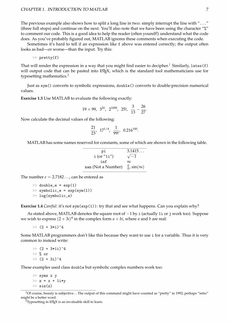
MATLAB has some names reserved for constants, some of which are shown in the following table.
pi 3.1415 . . .i (or “1i”)
√−1
inf ∞nan (Not a Number) 0
0 , sin(∞)
The number e = 2.7182 . . ., can be entered as
>> double_e = exp(1)
>> symbolic_e = exp(sym(1))
>> log(symbolic_e)
Exercise 1.4 Careful: it’s not sym(exp(1)): try that and see what happens. Can you explain why?
As stated above, MATLAB denotes the square root of−1 by i (actually 1i or j work too). Supposewe wish to express (2 + 3i)4 in the complex form a + bi, where a and b are real:
>> (2 + 3*i)^4
Some MATLAB programmers don’t like this because they want to use i for a variable. Thus it is verycommon to instead write:
>> (2 + 3*1i)^4
>> % or
>> (2 + 3i)^4
These examples used class double but symbolic complex numbers work too:
>> syms x y
>> z = x + 1i*y
>> sin(z)
1Of course, beauty is subjective. . . The output of this command might have counted as “pretty” in 1992; perhaps “retro”might be a better word.
2Typesetting in LATEX is an invaluable skill to learn.
CHAPTER 1. INTRODUCTION TO MATLAB 8
You might have a sense of unease at this point: you and I might be tacitly assuming x and y are realbut of course MATLAB doesn’t know that. Indeed the complex conjugate of z = x + iy is z = x− iybut MATLAB says:
>> syms x y
>> z = x + 1i*y
>> conj(z)
We will see how to fix this later using assumptions in Section 2.2.2.
Exercise 1.5 Use MATLAB to express the following in the approximate decimal form a + bi:
(5− 8i)2, i−1, i2, i12 ,
1 + i5 + 2i
,(
43+
2i5
)4
.
�
Exercise 1.6 Use symbolic complex numbers to verify that (a + bi)2 = a2 − b2 + 2abi. (Hint: oneapproach would be to construct the left-hand side and the right-hand side. Sometimes the simplify()command will give MATLAB a nudge. . . ). �
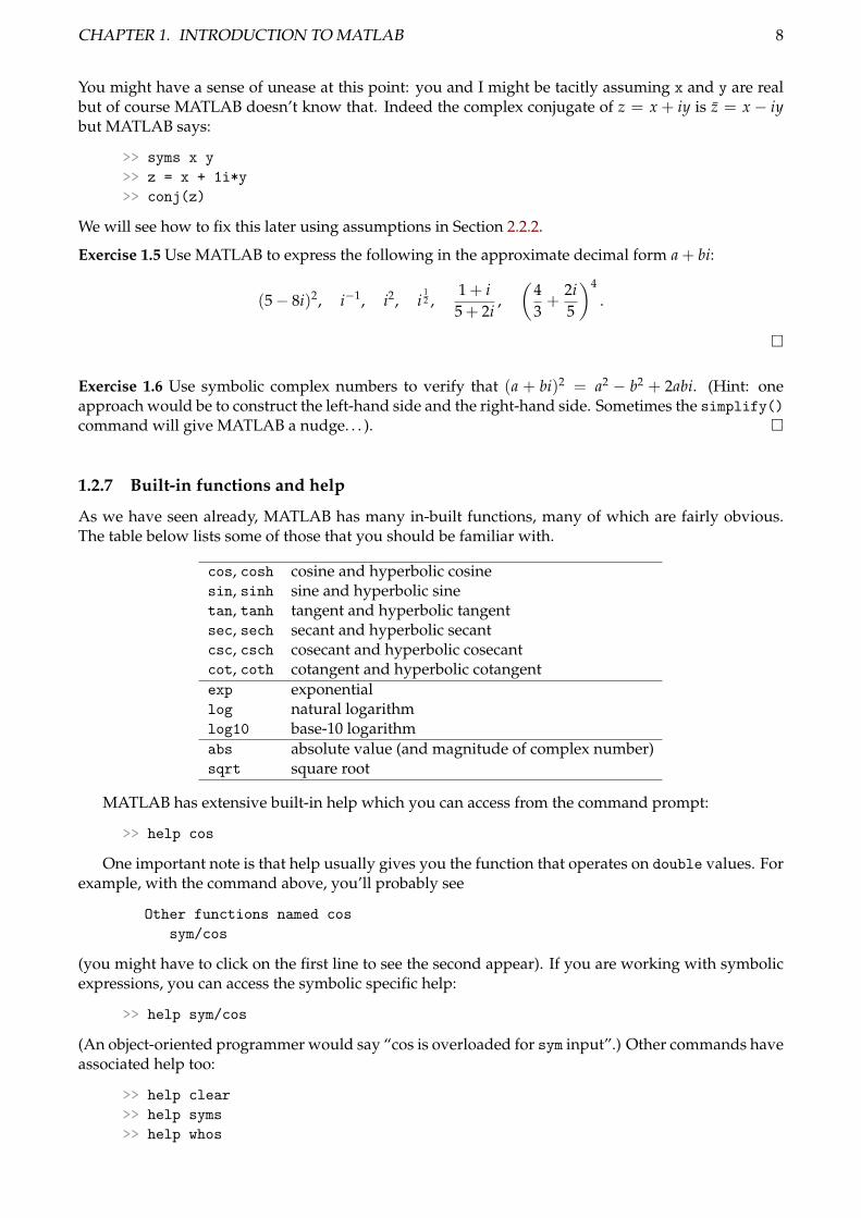
1.2.7 Built-in functions and help
As we have seen already, MATLAB has many in-built functions, many of which are fairly obvious.The table below lists some of those that you should be familiar with.
cos, cosh cosine and hyperbolic cosinesin, sinh sine and hyperbolic sinetan, tanh tangent and hyperbolic tangentsec, sech secant and hyperbolic secantcsc, csch cosecant and hyperbolic cosecantcot, coth cotangent and hyperbolic cotangentexp exponentiallog natural logarithmlog10 base-10 logarithmabs absolute value (and magnitude of complex number)sqrt square root
MATLAB has extensive built-in help which you can access from the command prompt:
>> help cos
One important note is that help usually gives you the function that operates on double values. Forexample, with the command above, you’ll probably see
Other functions named cos
sym/cos
(you might have to click on the first line to see the second appear). If you are working with symbolicexpressions, you can access the symbolic specific help:
>> help sym/cos
(An object-oriented programmer would say “cos is overloaded for sym input”.) Other commands haveassociated help too:
>> help clear
>> help syms
>> help whos
CHAPTER 1. INTRODUCTION TO MATLAB 9
You can also search for keywords:
>> lookfor hyperbolic
MATLAB has more detailed hyperlinked help accessed with the doc command (and also availableonline).
Exercise 1.7 Use MATLAB to evaluate the following:
tan2(π/3), sec(π/6), 1 + cot2(π/4), cosec2(π/4)e3 ln 4.
�
Exercise 1.8 Use the help facility to learn how to compute the binomial coefficient nCr in MATLAB.Evaluate 10C4 and 250C12. Do this both symbolically and numerically. Which is the incorrect answer?�
Exercise 1.9 Evaluate arcsin(1/2) and arcsin((√
5 + 1)/4). Evaluate sec(arctan x) in terms of x. �
1.3 2D graphics
One of the very useful features of MATLAB is the ease with which many different types of graphsmay be drawn. Most graphs are drawn with variants of the plot command, which has several forms,each with many optional arguments that determine the appearance of the resulting graph. Here weintroduce a few of the simplest forms. If at any time you wish to learn more, explore with MATLAB’shelp and doc pages.
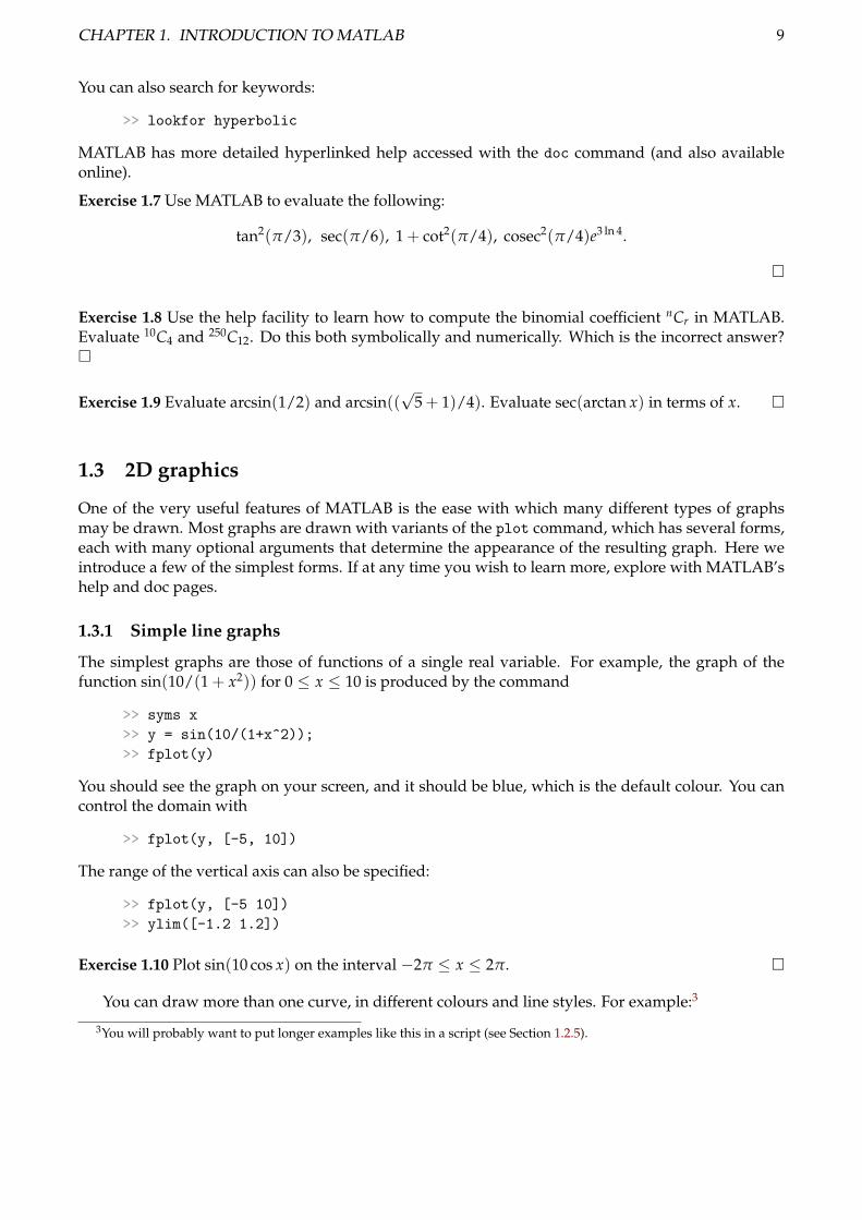
1.3.1 Simple line graphs
The simplest graphs are those of functions of a single real variable. For example, the graph of thefunction sin(10/(1 + x2)) for 0 ≤ x ≤ 10 is produced by the command
>> syms x
>> y = sin(10/(1+x^2));
>> fplot(y)
You should see the graph on your screen, and it should be blue, which is the default colour. You cancontrol the domain with
>> fplot(y, [-5, 10])
The range of the vertical axis can also be specified:
>> fplot(y, [-5 10])
>> ylim([-1.2 1.2])
Exercise 1.10 Plot sin(10 cos x) on the interval −2π ≤ x ≤ 2π. �
You can draw more than one curve, in different colours and line styles. For example:3
3You will probably want to put longer examples like this in a script (see Section 1.2.5).
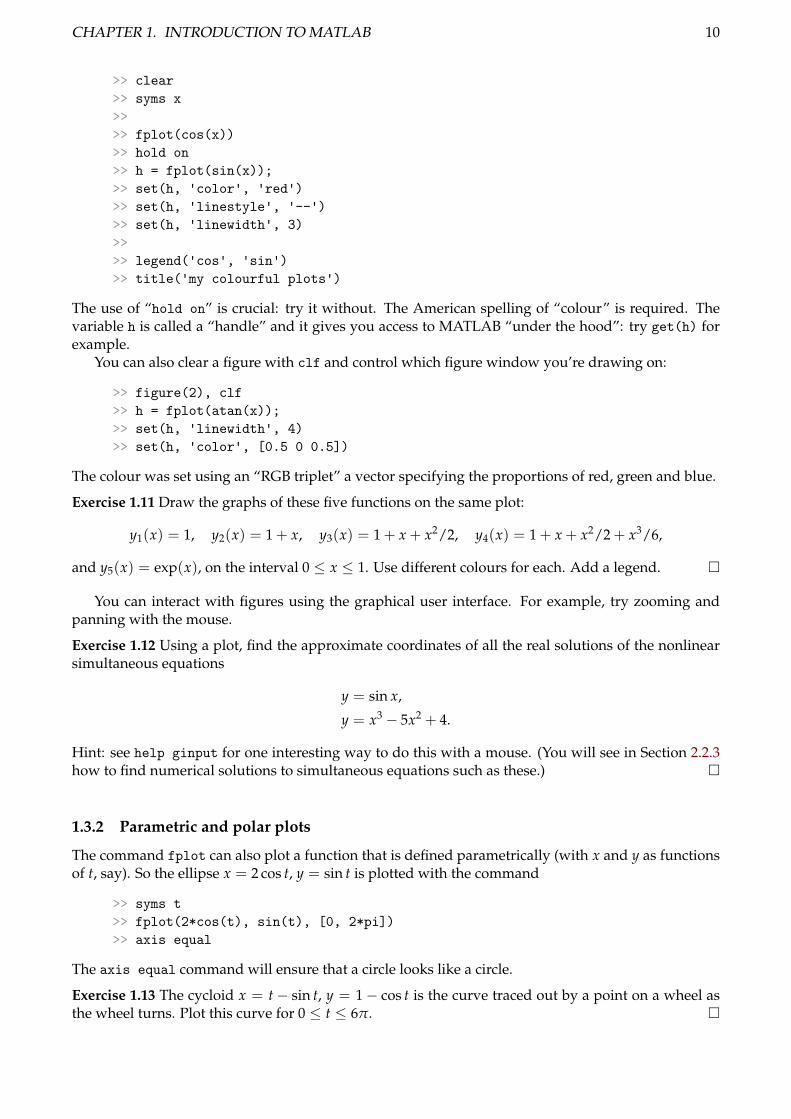
CHAPTER 1. INTRODUCTION TO MATLAB 10
>> clear
>> syms x
>>
>> fplot(cos(x))
>> hold on
>> h = fplot(sin(x));
>> set(h, 'color', 'red')
>> set(h, 'linestyle', '--')
>> set(h, 'linewidth', 3)
>>
>> legend('cos', 'sin')
>> title('my colourful plots')
The use of “hold on” is crucial: try it without. The American spelling of “colour” is required. Thevariable h is called a “handle” and it gives you access to MATLAB “under the hood”: try get(h) forexample.
You can also clear a figure with clf and control which figure window you’re drawing on:
>> figure(2), clf
>> h = fplot(atan(x));
>> set(h, 'linewidth', 4)
>> set(h, 'color', [0.5 0 0.5])
The colour was set using an “RGB triplet” a vector specifying the proportions of red, green and blue.
Exercise 1.11 Draw the graphs of these five functions on the same plot:
y1(x) = 1, y2(x) = 1 + x, y3(x) = 1 + x + x2/2, y4(x) = 1 + x + x2/2 + x3/6,
and y5(x) = exp(x), on the interval 0 ≤ x ≤ 1. Use different colours for each. Add a legend. �
You can interact with figures using the graphical user interface. For example, try zooming andpanning with the mouse.
Exercise 1.12 Using a plot, find the approximate coordinates of all the real solutions of the nonlinearsimultaneous equations
y = sin x,
y = x3 − 5x2 + 4.
Hint: see help ginput for one interesting way to do this with a mouse. (You will see in Section 2.2.3how to find numerical solutions to simultaneous equations such as these.) �
1.3.2 Parametric and polar plots
The command fplot can also plot a function that is defined parametrically (with x and y as functionsof t, say). So the ellipse x = 2 cos t, y = sin t is plotted with the command
>> syms t
>> fplot(2*cos(t), sin(t), [0, 2*pi])
>> axis equal
The axis equal command will ensure that a circle looks like a circle.
Exercise 1.13 The cycloid x = t− sin t, y = 1− cos t is the curve traced out by a point on a wheel asthe wheel turns. Plot this curve for 0 ≤ t ≤ 6π. �
CHAPTER 1. INTRODUCTION TO MATLAB 11
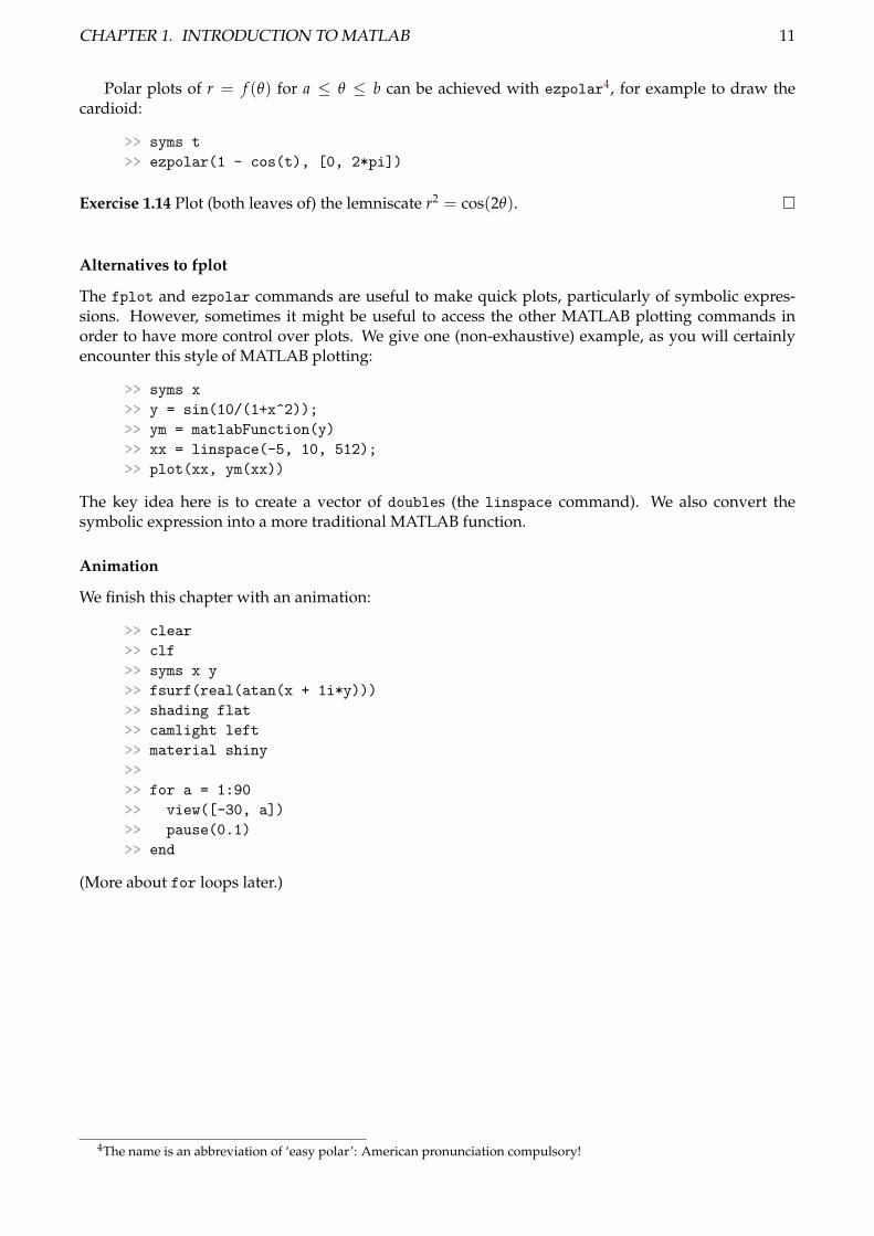
Polar plots of r = f (θ) for a ≤ θ ≤ b can be achieved with ezpolar4, for example to draw thecardioid:
>> syms t
>> ezpolar(1 - cos(t), [0, 2*pi])
Exercise 1.14 Plot (both leaves of) the lemniscate r2 = cos(2θ). �
Alternatives to fplot
The fplot and ezpolar commands are useful to make quick plots, particularly of symbolic expres-sions. However, sometimes it might be useful to access the other MATLAB plotting commands inorder to have more control over plots. We give one (non-exhaustive) example, as you will certainlyencounter this style of MATLAB plotting:
>> syms x
>> y = sin(10/(1+x^2));
>> ym = matlabFunction(y)
>> xx = linspace(-5, 10, 512);
>> plot(xx, ym(xx))
The key idea here is to create a vector of doubles (the linspace command). We also convert thesymbolic expression into a more traditional MATLAB function.
Animation
We finish this chapter with an animation:
>> clear
>> clf
>> syms x y
>> fsurf(real(atan(x + 1i*y)))
>> shading flat
>> camlight left
>> material shiny
>>
>> for a = 1:90
>> view([-30, a])
>> pause(0.1)
>> end
(More about for loops later.)
4The name is an abbreviation of ‘easy polar’: American pronunciation compulsory!
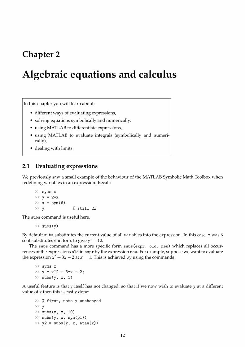
Chapter 2
Algebraic equations and calculus
In this chapter you will learn about:
• different ways of evaluating expressions,
• solving equations symbolically and numerically,
• using MATLAB to differentiate expressions,
• using MATLAB to evaluate integrals (symbolically and numeri-cally),
• dealing with limits.
2.1 Evaluating expressions
We previously saw a small example of the behaviour of the MATLAB Symbolic Math Toolbox whenredefining variables in an expression. Recall:
>> syms x
>> y = 2*x
>> x = sym(6)
>> y % still 2x
The subs command is useful here.
>> subs(y)
By default subs substitutes the current value of all variables into the expression. In this case, x was 6so it substitutes 6 in for x to give y = 12.
The subs command has a more specific form subs(expr, old, new) which replaces all occur-rences of the expressions old in expr by the expression new. For example, suppose we want to evaluatethe expression x2 + 3x− 2 at x = 1. This is achieved by using the commands
>> syms x
>> y = x^2 + 3*x - 2;
>> subs(y, x, 1)
A useful feature is that y itself has not changed, so that if we now wish to evaluate y at a differentvalue of x then this is easily done:
>> % first, note y unchanged
>> y
>> subs(y, x, 10)
>> subs(y, x, sym(pi))
>> y2 = subs(y, x, atan(x))
12
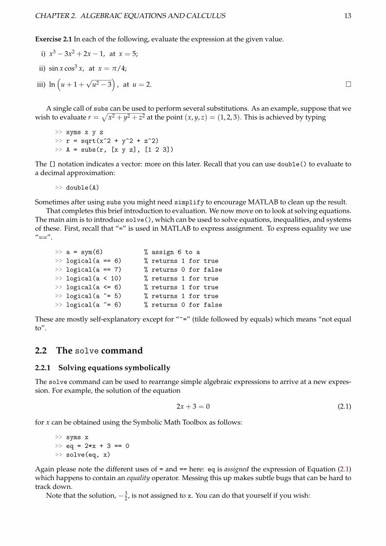
CHAPTER 2. ALGEBRAIC EQUATIONS AND CALCULUS 13
Exercise 2.1 In each of the following, evaluate the expression at the given value.
i) x3 − 3x2 + 2x− 1, at x = 5;
ii) sin x cos3 x, at x = π/4;
iii) ln(
u + 1 +√
u2 − 3)
, at u = 2. �
A single call of subs can be used to perform several substitutions. As an example, suppose that wewish to evaluate r =
√x2 + y2 + z2 at the point (x, y, z) = (1, 2, 3). This is achieved by typing
>> syms x y z
>> r = sqrt(x^2 + y^2 + z^2)
>> A = subs(r, [x y z], [1 2 3])
The [] notation indicates a vector: more on this later. Recall that you can use double() to evaluate toa decimal approximation:
>> double(A)
Sometimes after using subs you might need simplify to encourage MATLAB to clean up the result.That completes this brief introduction to evaluation. We now move on to look at solving equations.
The main aim is to introduce solve(), which can be used to solve equations, inequalities, and systemsof these. First, recall that “=” is used in MATLAB to express assignment. To express equality we use“==”.
>> a = sym(6) % assign 6 to a
>> logical(a == 6) % returns 1 for true
>> logical(a == 7) % returns 0 for false
>> logical(a < 10) % returns 1 for true
>> logical(a <= 6) % returns 1 for true
>> logical(a ~= 5) % returns 1 for true
>> logical(a ~= 6) % returns 0 for false
These are mostly self-explanatory except for “~=” (tilde followed by equals) which means “not equalto”.
2.2 The solve command
2.2.1 Solving equations symbolically
The solve command can be used to rearrange simple algebraic expressions to arrive at a new expres-sion. For example, the solution of the equation
2x + 3 = 0 (2.1)
for x can be obtained using the Symbolic Math Toolbox as follows:
>> syms x
>> eq = 2*x + 3 == 0
>> solve(eq, x)
Again please note the different uses of = and == here: eq is assigned the expression of Equation (2.1)which happens to contain an equality operator. Messing this up makes subtle bugs that can be hard totrack down.
Note that the solution, − 32 , is not assigned to x. You can do that yourself if you wish:
CHAPTER 2. ALGEBRAIC EQUATIONS AND CALCULUS 14
>> x
>> x = solve(eq, x)
>> eq
>> eq2 = subs(eq)
Suppose that we wish to solve the simultaneous equations
x + y = 2, −x + 3y = 3.
This is done as follows:
>> clear
>> syms x y
>> eq1 = x+y == 2;
>> eq2 = -x+3*y == 3;
>> [xsoln, ysoln] = solve(eq1, eq2, x, y)
An alternative:
>> sol = solve(eq1, eq2, x, y)
>> xsoln = sol.x
>> ysoln = sol.y
where sol is something called a structure: roughly speaking it can contain “sub-variables” known asfields.
What about problems with multiple solutions?
>> clear
>> syms x
>> eqn = x^2 == -25
>> sol = solve(eqn, x)
>> sol(1)
>> sol(2)
Here sol is a vector of two solutions, −5i and 5i.
Exercise 2.2 Find the solutions of the following equations:
(a) x2 − x− 2025 = 0, (b) x3 − 6x2 − 19x + 24 = 0,
(c) 2x4 − 11x3 − 20x2 + 113x + 60 = 0. �
Exercise 2.3 Use the solve command to find the point of intersection, in the (x, y)-plane, of the twolines
ax + by = A, cx + dy = B.
Having found the intersection, find an expression for the distance of the point of intersection from theorigin. �
Note that in the previous exercise the Symbolic Math Toolbox made various assumptions (for ex-ample that ad − bc 6= 0). Some other systems are very good at finding a wider variety of solutionpossibilities. This can be useful (and/or annoying) depending on what you’re trying to accomplish.
2.2.2 Assumptions
Sometimes one makes assumptions about equations and variables. For example, you might be inter-ested only in the real roots of a quadratic. Or you might have a mathematical model where you know aparticular variable must stay positive (say it represents a positive physical quantity like concentrationor density). The Symbolic Math Toolbox allows you to add assumptions to symbolic variables.
CHAPTER 2. ALGEBRAIC EQUATIONS AND CALCULUS 15
>> syms x
>> assume(x, 'real')
>> ineq = x^2 <= 25
>> S = solve(ineq, x, 'ReturnConditions', true);
>> S.conditions
>> assumeAlso(x > 0)
>> S = solve(ineq, x, 'ReturnConditions', true);
>> S.conditions
>> ineq = x^2 <= -25
>> S = solve(ineq, x, 'ReturnConditions', true);
>> S.conditions
To list the current assumptions, type:
>> assumptions
You can remove the assumptions on a particular variable using
>> x = sym('x', 'clear')
Recall that if you want to clear everything and start again, the usual approach is the clear command.But it is worth mentioning that this might not remove assumptions from variables.1 The clear all
command will do the right thing.
Exercise 2.4 Define z = x + iy where x and y are symbolic variables. Take the complex conjugate of z.Now modify your code to assume that both x and y are real and run your code again. �
2.2.3 Solving equations numerically
The solve command is used for finding symbolic solutions to equations. This is not always possible,but numerical (approximate) solutions can usually be found. If solve is unable to find a symbolicsolution, it will try to find a numerical solution.
For example, suppose we wish to solve the equation
sin x = x3 − 5x2 + 4,
and that having plotted the graphs of sin x and x3 − 5x2 + 4 we know that there are three solutions, atapproximately x = −0.90, 0.89 and 4.78 (these approximate solutions were obtained in Exercise 1.12).
To find these solution more precisely, we try solve:
>> clear
>> syms x
>> eqn = sin(x) == x^3 - 5*x^2 + 4;
>> solve(eqn, x)
This fails to find an exact symbolic solution but it finds a numerical solution
ans =
0.88543649189409090795806224578236
If you’re going to do something else with the result, you probably want:
>> y = double(solve(eqn, x))
which converts it to a double.What about the other two solutions? The most common numerical approaches involve providing
either an interval in which to search or an initial guess. Here we outline two possible approaches.
1The variable might be deleted but not the assumption, possibly leading to very subtle and hard-to-find bugs. Deter-mining whether the assumption will remain or not depends on the MATLAB release that you are using, and the way youredefine your new variables after having deleted them (the commands syms x or x = sym(’x’) might in this case behavedifferently).
CHAPTER 2. ALGEBRAIC EQUATIONS AND CALCULUS 16
The vpasolve command The Symbolic Math Toolbox also has the command vpasolve, which uses“variable-precision arithmetic” (see Appendix B.2 for more information.) One way to use this com-mand is to provide a search interval:
>> vpasolve(eqn, x, [-1 0])
>> vpasolve(eqn, x, [0 1])
>> vpasolve(eqn, x, [4 5])
ans =
-0.90040020886787653209849187387426
ans =
0.88543649189409090795806224578236
ans =
4.7813983927628242128187791632837
Alternatively, you can provide an initial guess:
>> vpasolve(eqn, x, -.9)
>> vpasolve(eqn, x, .8)
>> y = double(vpasolve(eqn, x, 4.7))
The last example includes conversion to double, assuming the solution is to be used in further calcu-lations.
Note that the vpasolve command does not respect assumptions on variables.
Alternative approach: fzero for numerical root finding The MATLAB command fzero() doesroot-finding: it searches for numerical solutions of f (x) = 0 where f is a function of one variable.
>> f = @(x) sin(x) - ( x^3 - 5*x^2 + 4 );
>> format long
>> fzero(f, -1)
ans =
-0.900400208867877
Some explanation: the first line creates a MATLAB “anonymous function” (see Appendix B.1), whichis then passed to fzero, along with an initial guess. We can then find the third root:
>> fzero(f, 5)
ans =
4.781398392762824
Note that fzero does not work with symbolic expressions or symbolic functions.Having to enter the same expression again takes time and risks introducing an error. Here’s one
approach to converting the symbolic equation “eqn” from above into an appropriate function f:
>> % we want the left-hand-side and right-hand-side
>> LR = children(eqn)
>> f = matlabFunction(LR(1) - LR(2))
>> fzero(f, -1)
ans =
-0.900400208867877
Exercise 2.5 Make a plot showing the roots of x3 + 3x2 − 2x + 1. Then use solve() to find the roots.Use double() to find numerical approximations to the roots. �
CHAPTER 2. ALGEBRAIC EQUATIONS AND CALCULUS 17
Exercise 2.6 Find real solutions of the equation
x sin x =12
for x in the following ranges: (i) 0 < x < 2; (ii) 2 < x < 4; (iii) 6 < x < 7; (iv) 8 < x < 10. Verifygraphically that there are no solutions in the range 4 < x < 6. �
2.3 Differentiation and the diff command
The Symbolic Math Toolbox can find the derivatives of expressions of one or several variables. In thissection we introduce the diff command, which is the basic differentiation operator for expressions,and illustrate its use in different situations including finding the coordinates of stationary points.
We start with an example: the derivative of sin x with respect to x is found with the command
>> syms x
>> diff(sin(x), x)
The general syntax for differentiating an expression expr with respect to a variable var is
>> diff(expr, var);
and the derivative of ex2+a2with respect to x is found with the commands
>> syms x a
>> z = exp(x^2 + a^2);
>> d1 = diff(z, x)
The second derivative of ex2+a2with respect to x is
>> diff(d1, x)
and this same result can also be found all in one go by typing
>> diff(z, x, 2)
So the fifth derivative of sin(x2) is achieved by
>> diff(sin(x^2), x, 5)
Partial differentiation2 of expressions of more than one variable is performed by a straightforwardextension of this procedure. For example, consider the expression sin x cos y. Its second derivativescan be found as follows. First define z = sin x cos y:
>> syms x y
>> z = sin(x)*cos(y)
Then the second derivative ∂2z/∂x2 is given by
>> diff(z, x, 2)
and ∂2z/∂y2 is found with
>> diff(z, y, 2)
or by nesting the diff command
>> diff(diff(z, y), y)
Thus one way to evaluate the mixed second derivative ∂2z∂x∂y is:
2This topic may be new to you; it will be covered in lectures this term.
CHAPTER 2. ALGEBRAIC EQUATIONS AND CALCULUS 18
>> diff(diff(z, x), y)
This is a bit cumbersome, particularly if you want something like ∂5z∂x2∂y3 , and instead you can do:
>> diff(z, x, x, y, y, y)
For example, we can verify that the order of differentiation does not matter here:
>> diff(z, y, x)
>> diff(z, x, y)
Sometimes it is necessary to find the derivative of an expression at a particular point, rather thanas a function of the independent variable(s). This is achieved with a combination of the diff, subsand sometimes double commands. Thus the value of the first derivative of sin x at x = 6 is given bythe commands
>> f = diff(sin(x), x);
>> subs(f, x, 6)
and to get a decimal approximation:
>> double(subs(f, x, 6))
The following exercises give practice in the diff command and also revise some earlier commandssuch as solve and plot.
Exercise 2.7 Findd
dx
((x2 + 1)4
e2x
)and evaluate it at x = 1. �
Exercise 2.8 Plot the second derivative of x4/(1 + x2) for −5 ≤ x ≤ 5. �
Exercise 2.9 Given y = 12x5 − 15x4 + 20x3 − 330x2 + 600x + 2, find the (x, y) coordinates of anystationary points (that is, those for which y′(x) = 0). Use MATLAB to plot y so that the real stationarypoints are visible. Can you also make a plot to show the complex stationary points? �
Exercise 2.10 If z = ln(x2 + y2) find the value of the constant a such that(∂z∂x
)2
+
(∂z∂y
)2
= ae−z.
�
Exercise 2.11 Execute this code:
>> diff(sym(5))
>> diff(5)
and explain the results (hint: what does diff([1 2 5 9]) do?). �
CHAPTER 2. ALGEBRAIC EQUATIONS AND CALCULUS 19
2.3.1 Differentiation of unknown functions
So far only the derivatives of expressions with an explicit form (in terms of one or more independentvariables) have been found. In this section we look at how to differentiate arbitrary functions, say y(x)or f (x, y), without first giving them an explicit form. For example, we might want to find dy/dx (as afunction of y and x) given that x2 + y2 = 3. However, typing
>> syms x y
>> diff(y, x)
returns 0 because MATLAB does not know that we intended y to depend on x; x and y are free inde-pendent variables and are treated as such.
This difficulty is addressed in the Symbolic Math Toolbox by using y(x); MATLAB interprets thissyntax to mean that y(x) depends on x. Thus we have
>> clear
>> syms y(x)
>> diff(y,x)
>> diff(y,x,2)
Note here the syms y(x) also makes x a symbolic variable.
Differentiation and the “symfun”
The syntax here is quite important. Note the difference
>> syms g(x)
>> A = diff(g, x) % yes, A is a symfun for the deriv
>> B = diff(g(x), x) % gives an expression, not a symfun
>> whos A B
The distinction between an expression and a symfun is usually not important, but in some cases—such as dealing with differential equations—it makes an important difference.
Functions of multiple variables can also be manipulated using symfuns:
>> syms f(x,y)
>> f
>> diff(f, x)
>> diff(f, x, 2)
>> diff(f, x, y)
>> diff(f, x, x, y, y, y)
Using symfuns, the diff command knows the usual rules of differentiation, for instance the addi-tion, multiplication and quotient rules:
>> syms f(x) g(x)
>> diff(f + g, x)
>> diff(f * g, x)
>> diff(f / g, x)
To illustrate an application of this theory, suppose that we wish to find dy/dx (in terms of x and y)given that x2 + y2 = 3. To do this with MATLAB, first define the given explicit equation by typing
>> clear
>> syms y(x)
>> eq1 = x^2 + y(x)^2 == 3
and then differentiate this equation, assigning the output equation to a new name
>> eq2 = diff(eq1, x)
CHAPTER 2. ALGEBRAIC EQUATIONS AND CALCULUS 20
Let’s ask MATLAB to solve the resulting expression for dy/dx:
>> solve(eq2, diff(y, x)) % fail
>> solve(eq2, diff(y(x), x)) % fail
Hmm, we’ll have to try a bit harder:
>> % use subs to replace the deriv with "dydx"
>> syms dydx
>> eq3 = subs(eq2, diff(y(x), x), dydx)
>> % now solve for dydx
>> solve(eq3, dydx)
Exercise 2.12 Find the derivatives of
sin f (x), sin(
e f (x))
, exp(√
1 + f (x)g(x))
.
�
Exercise 2.13 Find dz/dp implicitly (in terms of z and p) given that
p3 + z(p)2 + 3pz(p) = 0.
Try to convince MATLAB to isolate dz/dp, that is, solve for dz/dp. �
2.4 Evaluating limits
This short section introduces the command limit. Its syntax is fairly self-explanatory. For example,to find
limx→0
sin xx
type
>> syms x
>> limit(sin(x)/x, x, 0)
Left and right limits can also be found. For example, to find
limx→3+
x2 − 4x2 − 5x + 6
use the command
>> syms x
>> expr = (x^2-4)/(x^2-5*x+6);
>> limit(expr, x, 3, 'right')
Exercise 2.14 Use MATLAB to evaluate the following limits
(i) limx→0
tan x− xx− sin x
, (ii) limx→∞
(1 +
1x
)x
.
In each case, make a plot that clearly demonstrates that the limits are correct. �
CHAPTER 2. ALGEBRAIC EQUATIONS AND CALCULUS 21
2.5 Integration
The Symbolic Math Toolbox can evaluate many integrals symbolically, and MATLAB itself can alsoprovide numerical estimates of most definite integrals.
2.5.1 The int operator
The syntax for integrating an expression expr with respect to a variable var is int(expr,var). Forexample, to integrate the expression xeax2
with respect to x type
>> syms x a
>> int(x*exp(a*x^2), x)
Note that the Symbolic Math Toolbox does not include the arbitrary constant of integration. To evalu-ate the definite integral ∫ 1
0xe5x2
dx
type
>> int(x*exp(5*x^2), x, 0, 1)
and to evaluate ∫ u
0
dx√u− x
type
>> syms x u
>> int(1/sqrt(u-x), x, 0, u)
If the Symbolic Math Toolbox cannot evaluate an integral, it returns a representation of the integralitself:
>> int(x^x, x)
which is a correct answer but probably not what you were hoping for!At this point you should experiment with some integrals just to see what can be done.
Exercise 2.15 Use MATLAB to integrate the following expressions with respect to x:
(i)√
ex − 1, (ii) x2(ax + b)5/2, (iii) sinh(6x) sinh4(x), (iv) cosh−6(x), (v) sin(ln(x)),
where a and b are constants. �
Exercise 2.16 Use MATLAB to evaluate the following expressions symbolically:
(i)∫ 1
1/2
11 + x3 dx, (ii)
∫ 1
0x2 tan−1 x dx, (iii)
∫ ∞
0
1(1 + x)(1 + x2)
dx. �
From these exercises you will note that the symbolic toolbox can deal with rather nasty integralssymbolically, and that it easily evaluates many of the integrals found in elementary texts or standardtables.
Nevertheless one often encounters integrals where it is desirable to have MATLAB evaluate an in-tegral numerically—for example, because the Symbolic Math Toolbox fails to integrate or the symboliccalculation is too slow.
CHAPTER 2. ALGEBRAIC EQUATIONS AND CALCULUS 22
2.5.2 Quadrature: numerical evaluation of integrals
You may be aware that the majority of integrals cannot be evaluated symbolically. If the symbolictoolbox fails to find a symbolic answer to a definite integral, or if you know that the integral in questioncannot be evaluated in terms of known functions, then it may be necessary to evaluate it numerically.
For example, suppose we try to integrate∫ 1
0 e−t arcsin(t)dt, symbolically by typing
>> syms t
>> y = exp(-t)*asin(t);
>> z = int(y, t, 0, 1)
As we noted before, this returns the symbolic integral expression; the Symbolic Math Toolbox doesnot know the answer. MATLAB has a variety of commands for doing numerical integration. This isknown as quadrature. These are independent of the symbolic toolbox, so we first convert out expressionto a MATLAB function and call integral(). Continuing our example above:
>> ym = matlabFunction(y);
>> z = integral(ym, 0, 1)
The integral command has various accuracy options: see help integral.To summarize, the int() command is part of the Symbolic Math Toolbox, and tries to evaluate
integrals symbolically; the integral() command is a MATLAB command which evaluates integralsnumerically using quadrature.
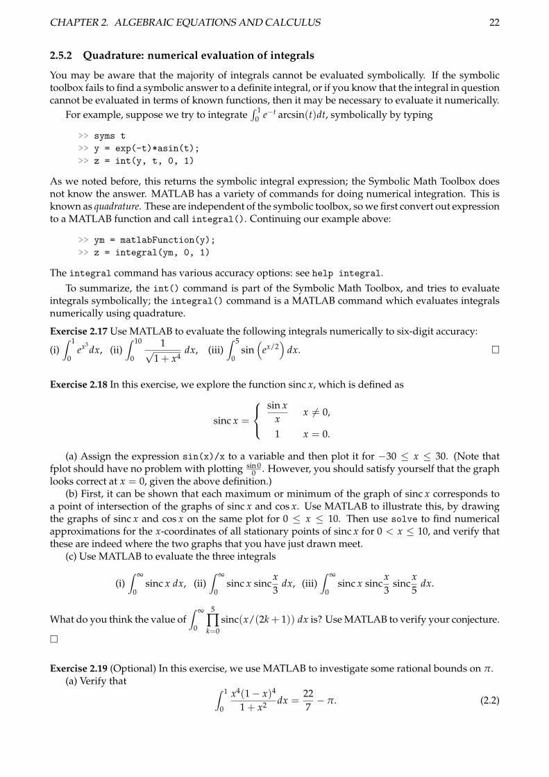
Exercise 2.17 Use MATLAB to evaluate the following integrals numerically to six-digit accuracy:
(i)∫ 1
0ex3
dx, (ii)∫ 10
0
1√1 + x4
dx, (iii)∫ 5
0sin(
ex/2)
dx. �
Exercise 2.18 In this exercise, we explore the function sinc x, which is defined as
sinc x =
sin x
xx 6= 0,
1 x = 0.
(a) Assign the expression sin(x)/x to a variable and then plot it for −30 ≤ x ≤ 30. (Note thatfplot should have no problem with plotting sin 0
0 . However, you should satisfy yourself that the graphlooks correct at x = 0, given the above definition.)
(b) First, it can be shown that each maximum or minimum of the graph of sinc x corresponds toa point of intersection of the graphs of sinc x and cos x. Use MATLAB to illustrate this, by drawingthe graphs of sinc x and cos x on the same plot for 0 ≤ x ≤ 10. Then use solve to find numericalapproximations for the x-coordinates of all stationary points of sinc x for 0 < x ≤ 10, and verify thatthese are indeed where the two graphs that you have just drawn meet.
(c) Use MATLAB to evaluate the three integrals
(i)∫ ∞
0sinc x dx, (ii)
∫ ∞
0sinc x sinc
x3
dx, (iii)∫ ∞
0sinc x sinc
x3
sincx5
dx.
What do you think the value of∫ ∞
0
5
∏k=0
sinc(x/(2k + 1)) dx is? Use MATLAB to verify your conjecture.
�
Exercise 2.19 (Optional) In this exercise, we use MATLAB to investigate some rational bounds on π.(a) Verify that ∫ 1
0
x4(1− x)4
1 + x2 dx =227− π. (2.2)
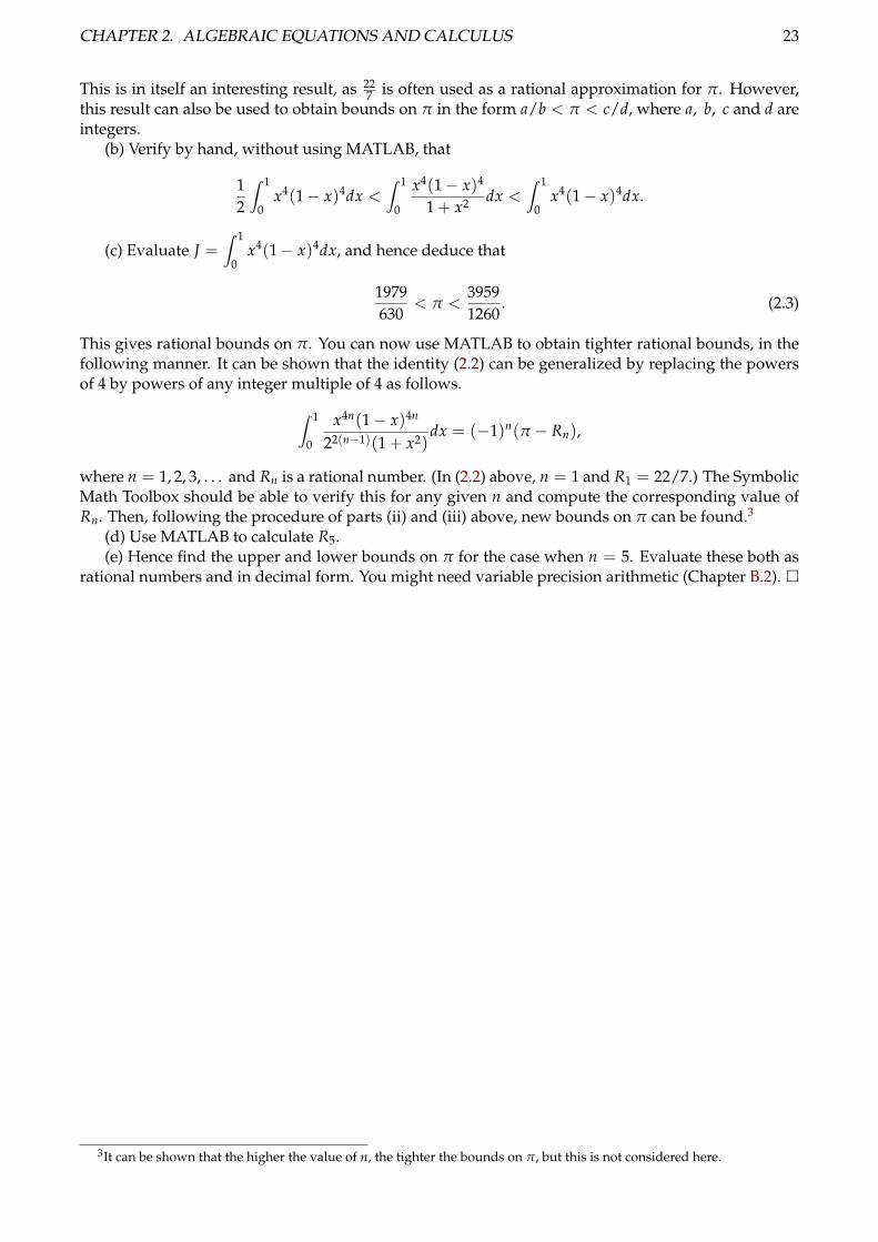
CHAPTER 2. ALGEBRAIC EQUATIONS AND CALCULUS 23
This is in itself an interesting result, as 227 is often used as a rational approximation for π. However,
this result can also be used to obtain bounds on π in the form a/b < π < c/d, where a, b, c and d areintegers.
(b) Verify by hand, without using MATLAB, that
12
∫ 1
0x4(1− x)4dx <
∫ 1
0
x4(1− x)4
1 + x2 dx <∫ 1
0x4(1− x)4dx.
(c) Evaluate J =∫ 1
0x4(1− x)4dx, and hence deduce that
1979630
< π <39591260
. (2.3)
This gives rational bounds on π. You can now use MATLAB to obtain tighter rational bounds, in thefollowing manner. It can be shown that the identity (2.2) can be generalized by replacing the powersof 4 by powers of any integer multiple of 4 as follows.∫ 1
0
x4n(1− x)4n
22(n−1)(1 + x2)dx = (−1)n(π − Rn),
where n = 1, 2, 3, . . . and Rn is a rational number. (In (2.2) above, n = 1 and R1 = 22/7.) The SymbolicMath Toolbox should be able to verify this for any given n and compute the corresponding value ofRn. Then, following the procedure of parts (ii) and (iii) above, new bounds on π can be found.3
(d) Use MATLAB to calculate R5.(e) Hence find the upper and lower bounds on π for the case when n = 5. Evaluate these both as
rational numbers and in decimal form. You might need variable precision arithmetic (Chapter B.2). �
3It can be shown that the higher the value of n, the tighter the bounds on π, but this is not considered here.
Chapter 3
Differential equations, sums, matrices andvectors
In this chapter you will learn about:
• solving differential equations,
• sums and products,
• the use of lists and vectors,
• 3D plotting.
3.1 Solving ordinary differential equations using dsolve
The “dsolve” command can be used to find the closed form solutions of many types of differentialequations. For example, to solve the homogeneous differential equation
d2ydx2 − y = 0
we use the symfun class as follows:
>> syms y(x)
>> ode = diff(y,x,2) - y == 0
>> dsolve(ode)
Notice the way by which the symbolic toolbox gives the constants of integration. The importantthing here is that, to obtain a symfun result for the command dsolve, y(x) was created as a symfun
and diff(y,x) was used to create the ODE (not diff(y(x),x)). This is an example of the toolboxdifferentiating arbitrary functions, which was discussed in Section 2.3.1.
Inhomogeneous equations are no different. To solve
dydx
+yx= x2
type
>> clear
>> syms y(x)
>> ode = diff(y,x) + y/x == x^2
>> dsolve(ode)
Sometimes MATLAB does not automatically simplify the solution as much as it could. For exam-ple, the solution of
d3xdt3 − 3
d2xdt2 + 3
dxdt− x = 16e3t
24
CHAPTER 3. DIFFERENTIAL EQUATIONS, SUMS, MATRICES AND VECTORS 25
is found by typing
>> syms x(t)
>> ode = diff(x,t,3) - 3*diff(x,t,2) + 3*diff(x,t) - x == 16*exp(3*t)
>> soln = dsolve(ode)
>> simplify(soln)
To insert initial and/or boundary conditions in MATLAB, proceed as in the following examples. Thesolution of the boundary value problem
y′′ + 5y′ + 6y = 0, y(0) = 0, y(1) = 3
is found as follows:
>> syms y(x)
>> DE = diff(y,x,2) + 5*diff(y,x) + 6*y == 0
>> soln = dsolve(DE, y(0)==0, y(1)==3)
We could then plot the solution:
>> fplot(soln, [0 1])
>> ylim([0 6])
>> grid on
>> ylabel('y')
Now consider the initial value problem
y′′ = y, y(0) = 1, y′(0) = 0,
which could be solved as follows
>> syms y(t)
>> DE = diff(y,t,2) == y;
>> yp = diff(y,t);
>> Y = dsolve(DE, y(0)==1, yp(0)==0)
And again a plot:
>> Yp = diff(Y, t);
>> clf
>> fplot(Y, [0 2])
>> hold on
>> h = fplot(Yp, [0 2])
>> set(h, 'color', 'red', 'linestyle', '-.')
>> grid on
>> % note how we enter y'(x) here:
>> legend('y(x)', 'y''(x)')
Exercise 3.1 Use MATLAB to solve the following differential equations:
(i)d2ydx2 + 3
dydx
+ 4y = sin x, (ii)dydx
= 3xy, y(0) = 1.
In (ii), plot the solution. �
Exercise 3.2 Solve the differential equation y′′+ y = 0, subject to the initial conditions y(0) = a, y′(0) =b. Assign the result to a variable and then evaluate the solution at x = π. �
Students interested in Chebfun (not part of this course) may note that it is a very powerful andflexible tool for solving differential equations numerically, both initial- and boundary-value problems.See chapters 7 and 10 of the Chebfun Guide at www.chebfun.org, and in particular, try the graphicaluser interface chebgui. Also check out Appendix B, “100 more examples”, in the Chebfun-based textExploring ODEs, freely available online at https://people.maths.ox.ac.uk/trefethen/ExplODE/.
CHAPTER 3. DIFFERENTIAL EQUATIONS, SUMS, MATRICES AND VECTORS 26
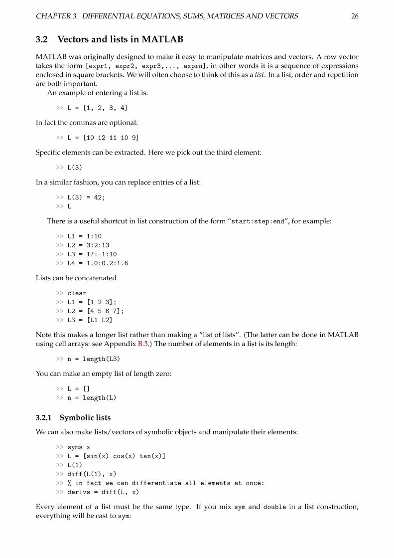
3.2 Vectors and lists in MATLAB
MATLAB was originally designed to make it easy to manipulate matrices and vectors. A row vectortakes the form [expr1, expr2, expr3,..., exprn], in other words it is a sequence of expressionsenclosed in square brackets. We will often choose to think of this as a list. In a list, order and repetitionare both important.
An example of entering a list is:
>> L = [1, 2, 3, 4]
In fact the commas are optional:
>> L = [10 12 11 10 9]
Specific elements can be extracted. Here we pick out the third element:
>> L(3)
In a similar fashion, you can replace entries of a list:
>> L(3) = 42;
>> L
There is a useful shortcut in list construction of the form “start:step:end”, for example:
>> L1 = 1:10
>> L2 = 3:2:13
>> L3 = 17:-1:10
>> L4 = 1.0:0.2:1.6
Lists can be concatenated
>> clear
>> L1 = [1 2 3];
>> L2 = [4 5 6 7];
>> L3 = [L1 L2]
Note this makes a longer list rather than making a “list of lists”. (The latter can be done in MATLABusing cell arrays: see Appendix B.3.) The number of elements in a list is its length:
>> n = length(L3)
You can make an empty list of length zero:
>> L = []
>> n = length(L)
3.2.1 Symbolic lists
We can also make lists/vectors of symbolic objects and manipulate their elements:
>> syms x
>> L = [sin(x) cos(x) tan(x)]
>> L(1)
>> diff(L(1), x)
>> % in fact we can differentiate all elements at once:
>> derivs = diff(L, x)
Every element of a list must be the same type. If you mix sym and double in a list construction,everything will be cast to sym:
CHAPTER 3. DIFFERENTIAL EQUATIONS, SUMS, MATRICES AND VECTORS 27
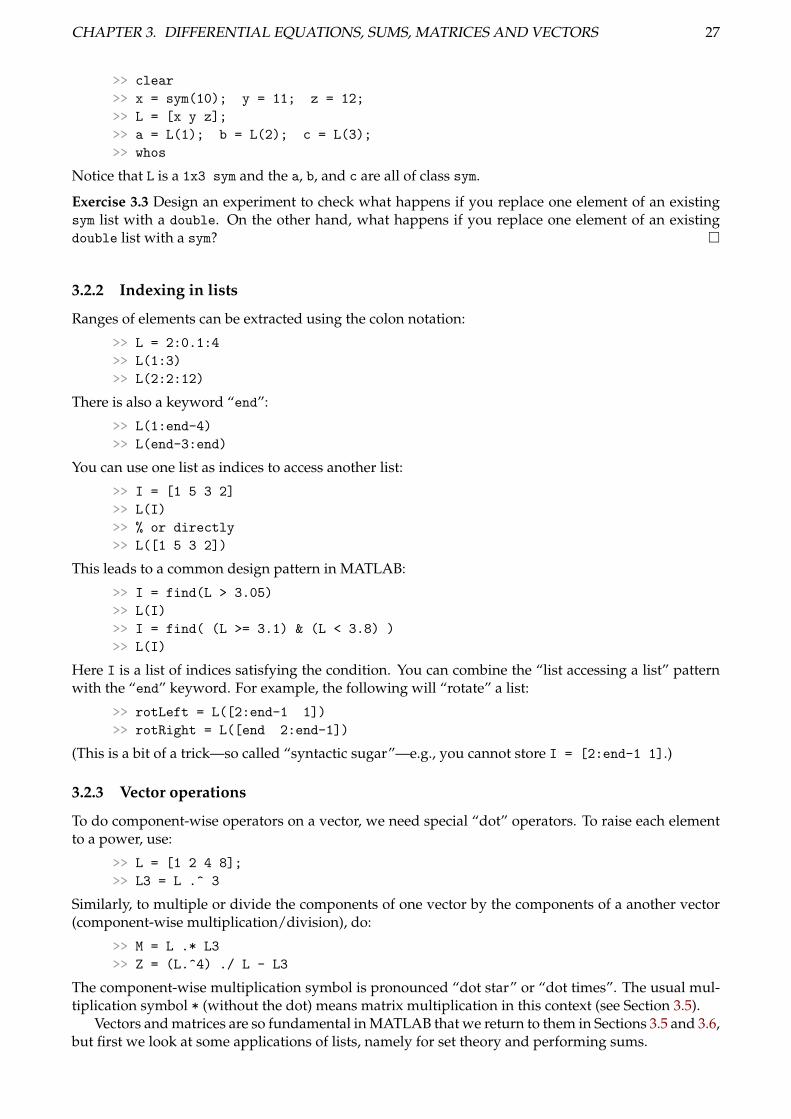
>> clear
>> x = sym(10); y = 11; z = 12;
>> L = [x y z];
>> a = L(1); b = L(2); c = L(3);
>> whos
Notice that L is a 1x3 sym and the a, b, and c are all of class sym.
Exercise 3.3 Design an experiment to check what happens if you replace one element of an existingsym list with a double. On the other hand, what happens if you replace one element of an existingdouble list with a sym? �
3.2.2 Indexing in lists
Ranges of elements can be extracted using the colon notation:
>> L = 2:0.1:4
>> L(1:3)
>> L(2:2:12)
There is also a keyword “end”:
>> L(1:end-4)
>> L(end-3:end)
You can use one list as indices to access another list:
>> I = [1 5 3 2]
>> L(I)
>> % or directly
>> L([1 5 3 2])
This leads to a common design pattern in MATLAB:
>> I = find(L > 3.05)
>> L(I)
>> I = find( (L >= 3.1) & (L < 3.8) )
>> L(I)
Here I is a list of indices satisfying the condition. You can combine the “list accessing a list” patternwith the “end” keyword. For example, the following will “rotate” a list:
>> rotLeft = L([2:end-1 1])
>> rotRight = L([end 2:end-1])
(This is a bit of a trick—so called “syntactic sugar”—e.g., you cannot store I = [2:end-1 1].)
3.2.3 Vector operations
To do component-wise operators on a vector, we need special “dot” operators. To raise each elementto a power, use:
>> L = [1 2 4 8];
>> L3 = L .^ 3
Similarly, to multiple or divide the components of one vector by the components of a another vector(component-wise multiplication/division), do:
>> M = L .* L3
>> Z = (L.^4) ./ L - L3
The component-wise multiplication symbol is pronounced “dot star” or “dot times”. The usual mul-tiplication symbol * (without the dot) means matrix multiplication in this context (see Section 3.5).
Vectors and matrices are so fundamental in MATLAB that we return to them in Sections 3.5 and 3.6,but first we look at some applications of lists, namely for set theory and performing sums.
CHAPTER 3. DIFFERENTIAL EQUATIONS, SUMS, MATRICES AND VECTORS 28
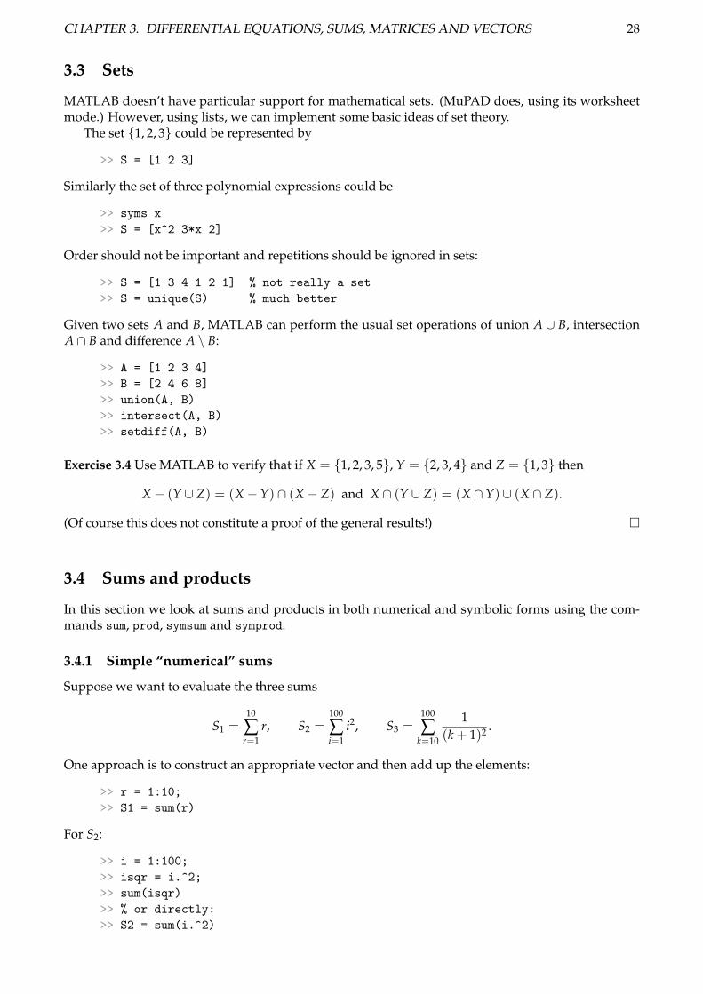
3.3 Sets
MATLAB doesn’t have particular support for mathematical sets. (MuPAD does, using its worksheetmode.) However, using lists, we can implement some basic ideas of set theory.
The set {1, 2, 3} could be represented by
>> S = [1 2 3]
Similarly the set of three polynomial expressions could be
>> syms x
>> S = [x^2 3*x 2]
Order should not be important and repetitions should be ignored in sets:
>> S = [1 3 4 1 2 1] % not really a set
>> S = unique(S) % much better
Given two sets A and B, MATLAB can perform the usual set operations of union A ∪ B, intersectionA ∩ B and difference A \ B:
>> A = [1 2 3 4]
>> B = [2 4 6 8]
>> union(A, B)
>> intersect(A, B)
>> setdiff(A, B)
Exercise 3.4 Use MATLAB to verify that if X = {1, 2, 3, 5}, Y = {2, 3, 4} and Z = {1, 3} then
X− (Y ∪ Z) = (X−Y) ∩ (X− Z) and X ∩ (Y ∪ Z) = (X ∩Y) ∪ (X ∩ Z).
(Of course this does not constitute a proof of the general results!) �
3.4 Sums and products
In this section we look at sums and products in both numerical and symbolic forms using the com-mands sum, prod, symsum and symprod.
3.4.1 Simple “numerical” sums
Suppose we want to evaluate the three sums
S1 =10
∑r=1
r, S2 =100
∑i=1
i2, S3 =100
∑k=10
1(k + 1)2 .
One approach is to construct an appropriate vector and then add up the elements:
>> r = 1:10;
>> S1 = sum(r)
For S2:
>> i = 1:100;
>> isqr = i.^2;
>> sum(isqr)
>> % or directly:
>> S2 = sum(i.^2)
CHAPTER 3. DIFFERENTIAL EQUATIONS, SUMS, MATRICES AND VECTORS 29
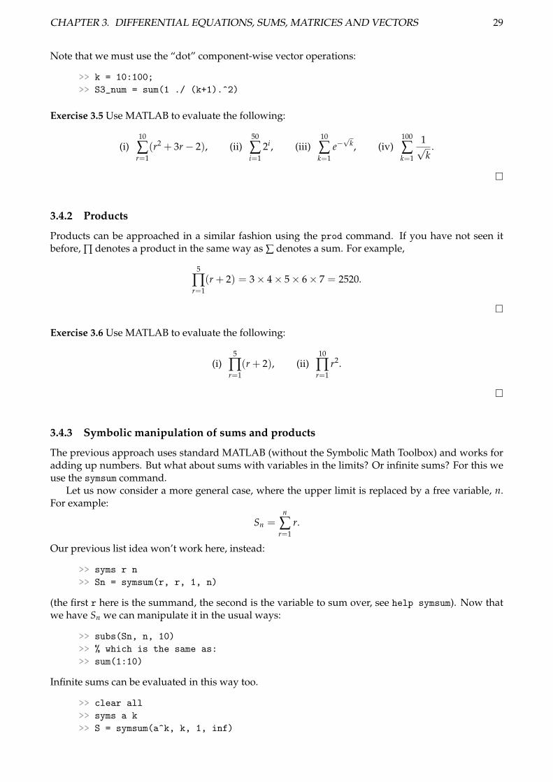
Note that we must use the “dot” component-wise vector operations:
>> k = 10:100;
>> S3_num = sum(1 ./ (k+1).^2)
Exercise 3.5 Use MATLAB to evaluate the following:
(i)10
∑r=1
(r2 + 3r− 2), (ii)50
∑i=1
2i, (iii)10
∑k=1
e−√
k, (iv)100
∑k=1
1√k
.
�
3.4.2 Products
Products can be approached in a similar fashion using the prod command. If you have not seen itbefore, ∏ denotes a product in the same way as ∑ denotes a sum. For example,
5
∏r=1
(r + 2) = 3× 4× 5× 6× 7 = 2520.
�
Exercise 3.6 Use MATLAB to evaluate the following:
(i)5
∏r=1
(r + 2), (ii)10
∏r=1
r2.
�
3.4.3 Symbolic manipulation of sums and products
The previous approach uses standard MATLAB (without the Symbolic Math Toolbox) and works foradding up numbers. But what about sums with variables in the limits? Or infinite sums? For this weuse the symsum command.
Let us now consider a more general case, where the upper limit is replaced by a free variable, n.For example:
Sn =n
∑r=1
r.
Our previous list idea won’t work here, instead:
>> syms r n
>> Sn = symsum(r, r, 1, n)
(the first r here is the summand, the second is the variable to sum over, see help symsum). Now thatwe have Sn we can manipulate it in the usual ways:
>> subs(Sn, n, 10)
>> % which is the same as:
>> sum(1:10)
Infinite sums can be evaluated in this way too.
>> clear all
>> syms a k
>> S = symsum(a^k, k, 1, inf)
CHAPTER 3. DIFFERENTIAL EQUATIONS, SUMS, MATRICES AND VECTORS 30
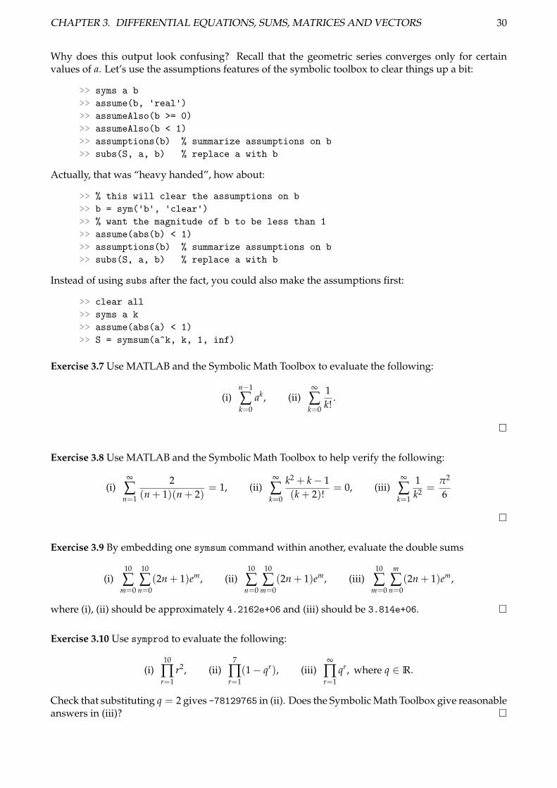
Why does this output look confusing? Recall that the geometric series converges only for certainvalues of a. Let’s use the assumptions features of the symbolic toolbox to clear things up a bit:
>> syms a b
>> assume(b, 'real')
>> assumeAlso(b >= 0)
>> assumeAlso(b < 1)
>> assumptions(b) % summarize assumptions on b
>> subs(S, a, b) % replace a with b
Actually, that was “heavy handed”, how about:
>> % this will clear the assumptions on b
>> b = sym('b', 'clear')
>> % want the magnitude of b to be less than 1
>> assume(abs(b) < 1)
>> assumptions(b) % summarize assumptions on b
>> subs(S, a, b) % replace a with b
Instead of using subs after the fact, you could also make the assumptions first:
>> clear all
>> syms a k
>> assume(abs(a) < 1)
>> S = symsum(a^k, k, 1, inf)
Exercise 3.7 Use MATLAB and the Symbolic Math Toolbox to evaluate the following:
(i)n−1
∑k=0
ak, (ii)∞
∑k=0
1k!
.
�
Exercise 3.8 Use MATLAB and the Symbolic Math Toolbox to help verify the following:
(i)∞
∑n=1
2(n + 1)(n + 2)
= 1, (ii)∞
∑k=0
k2 + k− 1(k + 2)!
= 0, (iii)∞
∑k=1
1k2 =
π2
6
�
Exercise 3.9 By embedding one symsum command within another, evaluate the double sums
(i)10
∑m=0
10
∑n=0
(2n + 1)em, (ii)10
∑n=0
10
∑m=0
(2n + 1)em, (iii)10
∑m=0
m
∑n=0
(2n + 1)em,
where (i), (ii) should be approximately 4.2162e+06 and (iii) should be 3.814e+06. �
Exercise 3.10 Use symprod to evaluate the following:
(i)10
∏r=1
r2, (ii)7
∏r=1
(1− qr), (iii)∞
∏r=1
qr, where q ∈ R.
Check that substituting q = 2 gives -78129765 in (ii). Does the Symbolic Math Toolbox give reasonableanswers in (iii)? �
CHAPTER 3. DIFFERENTIAL EQUATIONS, SUMS, MATRICES AND VECTORS 31
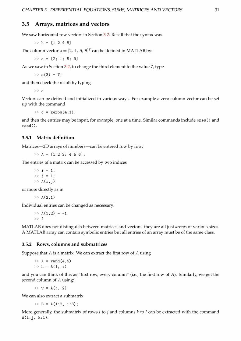
3.5 Arrays, matrices and vectors
We saw horizontal row vectors in Section 3.2. Recall that the syntax was
>> h = [1 2 4 8]
The column vector a = [2, 1, 5, 9]T can be defined in MATLAB by:
>> a = [2; 1; 5; 9]
As we saw in Section 3.2, to change the third element to the value 7, type
>> a(3) = 7;
and then check the result by typing
>> a
Vectors can be defined and initialized in various ways. For example a zero column vector can be setup with the command
>> c = zeros(4,1);
and then the entries may be input, for example, one at a time. Similar commands include ones() andrand().
3.5.1 Matrix definition
Matrices—2D arrays of numbers—can be entered row by row:
>> A = [1 2 3; 4 5 6];
The entries of a matrix can be accessed by two indices
>> i = 1;
>> j = 1;
>> A(i,j)
or more directly as in
>> A(2,1)
Individual entries can be changed as necessary:
>> A(1,2) = -1;
>> A
MATLAB does not distinguish between matrices and vectors: they are all just arrays of various sizes.A MATLAB array can contain symbolic entries but all entries of an array must be of the same class.
3.5.2 Rows, columns and submatrices
Suppose that A is a matrix. We can extract the first row of A using
>> A = rand(4,5)
>> h = A(1, :)
and you can think of this as “first row, every column” (i.e., the first row of A). Similarly, we get thesecond column of A using:
>> v = A(:, 2)
We can also extract a submatrix
>> B = A(1:2, 1:3);
More generally, the submatrix of rows i to j and columns k to l can be extracted with the commandA(i:j, k:l).
CHAPTER 3. DIFFERENTIAL EQUATIONS, SUMS, MATRICES AND VECTORS 32
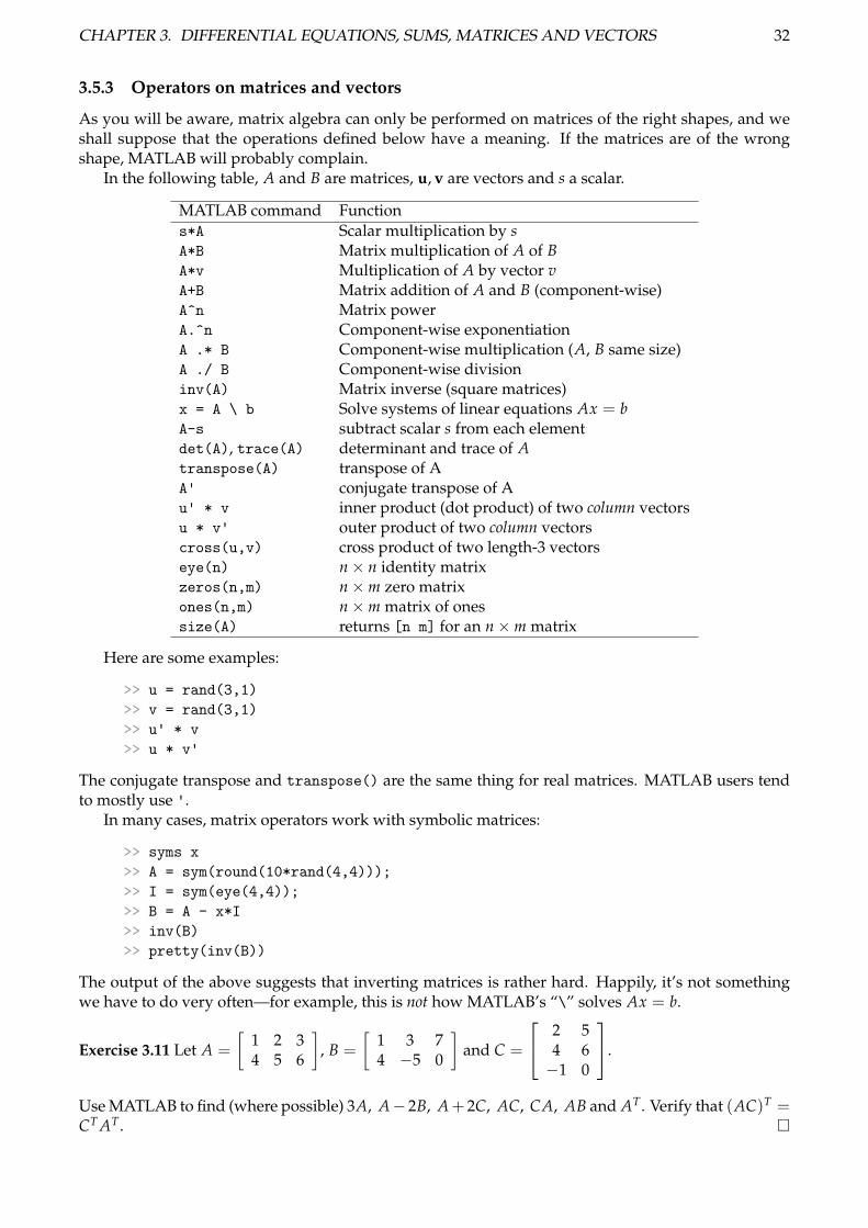
3.5.3 Operators on matrices and vectors
As you will be aware, matrix algebra can only be performed on matrices of the right shapes, and weshall suppose that the operations defined below have a meaning. If the matrices are of the wrongshape, MATLAB will probably complain.
In the following table, A and B are matrices, u, v are vectors and s a scalar.
MATLAB command Functions*A Scalar multiplication by sA*B Matrix multiplication of A of BA*v Multiplication of A by vector vA+B Matrix addition of A and B (component-wise)A^n Matrix powerA.^n Component-wise exponentiationA .* B Component-wise multiplication (A, B same size)A ./ B Component-wise divisioninv(A) Matrix inverse (square matrices)x = A \ b Solve systems of linear equations Ax = bA-s subtract scalar s from each elementdet(A), trace(A) determinant and trace of Atranspose(A) transpose of AA' conjugate transpose of Au' * v inner product (dot product) of two column vectorsu * v' outer product of two column vectorscross(u,v) cross product of two length-3 vectorseye(n) n× n identity matrixzeros(n,m) n×m zero matrixones(n,m) n×m matrix of onessize(A) returns [n m] for an n×m matrix
Here are some examples:
>> u = rand(3,1)
>> v = rand(3,1)
>> u' * v
>> u * v'
The conjugate transpose and transpose() are the same thing for real matrices. MATLAB users tendto mostly use '.
In many cases, matrix operators work with symbolic matrices:
>> syms x
>> A = sym(round(10*rand(4,4)));
>> I = sym(eye(4,4));
>> B = A - x*I
>> inv(B)
>> pretty(inv(B))
The output of the above suggests that inverting matrices is rather hard. Happily, it’s not somethingwe have to do very often—for example, this is not how MATLAB’s “\” solves Ax = b.
Exercise 3.11 Let A =
[1 2 34 5 6
], B =
[1 3 74 −5 0
]and C =
2 54 6−1 0
.
Use MATLAB to find (where possible) 3A, A− 2B, A+ 2C, AC, CA, AB and AT. Verify that (AC)T =CT AT. �
CHAPTER 3. DIFFERENTIAL EQUATIONS, SUMS, MATRICES AND VECTORS 33
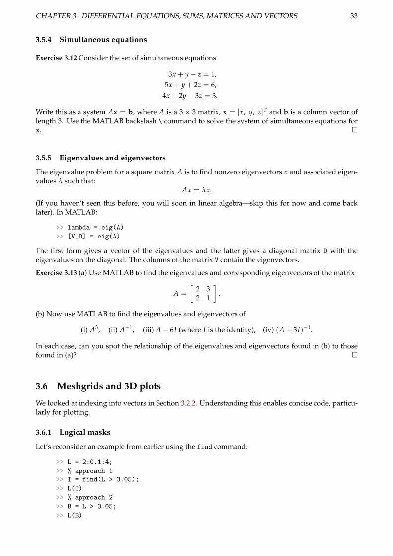
3.5.4 Simultaneous equations
Exercise 3.12 Consider the set of simultaneous equations
3x + y− z = 1,5x + y + 2z = 6,
4x− 2y− 3z = 3.
Write this as a system Ax = b, where A is a 3× 3 matrix, x = [x, y, z]T and b is a column vector oflength 3. Use the MATLAB backslash \ command to solve the system of simultaneous equations forx. �
3.5.5 Eigenvalues and eigenvectors
The eigenvalue problem for a square matrix A is to find nonzero eigenvectors x and associated eigen-values λ such that:
Ax = λx.
(If you haven’t seen this before, you will soon in linear algebra—skip this for now and come backlater). In MATLAB:
>> lambda = eig(A)
>> [V,D] = eig(A)
The first form gives a vector of the eigenvalues and the latter gives a diagonal matrix D with theeigenvalues on the diagonal. The columns of the matrix V contain the eigenvectors.
Exercise 3.13 (a) Use MATLAB to find the eigenvalues and corresponding eigenvectors of the matrix
A =
[2 32 1
].
(b) Now use MATLAB to find the eigenvalues and eigenvectors of
(i) A3, (ii) A−1, (iii) A− 6I (where I is the identity), (iv) (A + 3I)−1.
In each case, can you spot the relationship of the eigenvalues and eigenvectors found in (b) to thosefound in (a)? �
3.6 Meshgrids and 3D plots
We looked at indexing into vectors in Section 3.2.2. Understanding this enables concise code, particu-larly for plotting.
3.6.1 Logical masks
Let’s reconsider an example from earlier using the find command:
>> L = 2:0.1:4;
>> % approach 1
>> I = find(L > 3.05);
>> L(I)
>> % approach 2
>> B = L > 3.05;
>> L(B)
CHAPTER 3. DIFFERENTIAL EQUATIONS, SUMS, MATRICES AND VECTORS 34
The results of L(I) and L(B) are the same. But compare I and B. Note that I contains just the indicesof those elements which are greater than 3.05. On the other hand, B contains 1’s where the conditionis true and 0’s where it is false. B is known as a “logical mask”.
Here’s an example of what can be done with this sort of masking
>> x = linspace(-1, 1, 512);
>> y = cos(2*pi*x);
>> y(y > 0) = 0;
>> y(x > 0.5) = 2;
>> plot(x, y, 'b.-');
Exercise 3.14 Explain what each line of the previous job accomplishes. Change “512” in the abovecode to “20” and make the code explicitly display the two logical masks. If you swap the order of thetwo “y(...) = ...” lines, does the picture change? Why or why not? �
3.6.2 Meshgrid
We can build special 2D arrays (matrices) of x and y coordinates for use in plotting:
>> x = linspace(-2,2,60);
>> y = linspace(-1,1,40);
>> [xx,yy] = meshgrid(x,y);
>> f = sin(2*pi*xx) .* cos(pi*yy);
>>
>> figure(1), clf
>> surf(xx, yy, f);
>> axis equal
>> xlabel('x'), ylabel('y'), zlabel('f')
>>
>> figure(2), clf
>> pcolor(xx, yy, f);
>> axis equal, axis tight
>> xlabel('x'), ylabel('y')
>> colorbar
Meshgrid is essentially the Cartesian product of the 1D grids in the x and y directions. Examinethe following output to understand what meshgrid does:
>> x = linspace(-2, 2, 5)
>> y = linspace(-1, 1, 4)
>> [xx, yy] = meshgrid(x, y)
3.6.3 3D plotting
Exercise 3.15 In the plotting code above, try adding “shading interp”, “shading flat”, or“shading faceted” after each plot.
After the surf command, try adding these command one after another and examining what eachone does: “shading interp”, “camlight left”, “lighting phong”, “material shiny”.
Use your mouse and the rotate and zoom tools to interact with your figures. �
Next let’s combine meshgrids with logical masks. This gives a way to modify regions for plotting.
CHAPTER 3. DIFFERENTIAL EQUATIONS, SUMS, MATRICES AND VECTORS 35
>> x = linspace(-2,2,60);
>> y = linspace(-1,1,40);
>> [xx,yy] = meshgrid(x,y);
>> f = sin(2*pi*xx) .* cos(pi*yy);
>> I = (xx > 0) & (yy > 0);
>> f(I) = 0; % or try: f(I) = f(I)+1;
>>
>> figure(1), clf
>> surf(xx, yy, f);
>> axis equal
>> xlabel('x'), ylabel('y'), zlabel('f')
>>
>> figure(2), clf
>> pcolor(xx, yy, f);
>> axis equal, axis tight
>> xlabel('x'), ylabel('y')
>> colorbar
Exercise 3.16 Modify the above code so that for every point where f is negative, the value is replacedwith three times its absolute value.
Exercise 3.17 Modify the above code to plot f = 3− (x2 + y2) in the interior of the following triangle.Set f = 0 outside the triangle.
The interior of the triangle is defined by the inequalities
y < 0.25x + 0.5, x < 1.3 + 0.15y, and y > −0.4x− 0.5.
Also, try setting the outside values to inf and nan (not a number). �
Exercise 3.18 What does this code do?
>> A = rand(10,10);
>> I = A > 0.8;
>> A(~I) = 0;
�
Exercise 3.19 Plot the function besselj(nu,r) where r =√
x2 + y2 on a circle of radius 20 for variousinteger values of ν. Animate your plots over ν = 0, 1, 2, . . . using the pause command. �
Chapter 4
Loops, conditionals and functions
In this chapter you will learn about:
• using MATLAB loops and conditionals,
• writing functions in MATLAB,
• debugging programs.
In this chapter you will consolidate things you have learned so far and you will also be introducedto some simple programming techniques. The material here is very important and a lot of it will beneeded in the Hilary Term projects; it is therefore crucial that you start Hilary Term Week 3 havingcompleted Chapter 4.
In addition to being an environment for problem solving and exploring mathematics, MATLABis also a programming language. By this we mean that a series of command lines can be writtenwhich, when executed, perform a particular task. You have seen several simple programs already(and hopefully written a few too). In this chapter you will look at programming in more detail, todevelop longer and more structured command sequences. In particular you will look at some of themain building blocks of programming, namely loops, conditionals and functions.
4.1 Loops
Sometimes a MATLAB command (or a sequence of commands) may need to be executed a numberof times. The for. . .end control structure is provided for this purpose. For example, say we want tooutput the squares of the integers from 1 to 5. This can be achieved with the following command:
>> for j = 1:5
>> j^2
>> end
Essentially, any list can be provided in the “for j = ...” part, although you’ll find most frequentlyit is some set of integers.
>> for i = 1:2:7
>> i
>> end
>> for c = [4 7 1 4]
>> x = sym(pi)/4*c
>> s = sin(x)
>> end
As another example, a for loop could be used (instead of sum) to find the sum of the cubes of the evenintegers between 50 and 100 inclusive.
36
CHAPTER 4. LOOPS, CONDITIONALS AND FUNCTIONS 37
>> sumcubes = 0; % set sumcubes to zero initially
>> for i = 50:2:100
>> sumcubes = sumcubes + i^3;
>> end
>> sumcubes
Note also that the command within the loop has been indented. This makes the whole structure easierfor human beings to read (MATLAB doesn’t care).
Exercise 4.1 Use a for loop structure to plot cos(nπx/2) for n = 0, 1, 2, . . . 10. �
Exercise 4.2 Use one or more for loops to findN
∑n=1
(2n− 1)2 for each N = 5, 6, . . . , 30. �
Another form of loop is the “while” loop. For example, the sum-of-cubes-of-even-integers problemfrom above could be solved using a while loop as follows:
>> sumcubes = 0;
>> j = 50;
>>
>> while (j <= 100)
>> sumcubes = sumcubes + j^3;
>> j = j+2;
>> end
>> sumcubes
Exercise 4.3 In a while loop, is the condition—in the case above “(j<=100)”—checked before or aftereach iteration? �
4.1.1 Approximate solutions to equations
In this section the for...end structure is illustrated by looking at Newton’s method for finding ap-proximate solutions to equations of the form f (x) = 0. The process depends on the function being“approximately linear” when viewed on a small enough interval. (The First Year course should makethis more precise.)
Starting with a guess at the solution, a, the equation of the tangent through (a, f (a)) is
y− f (a)x− a
= f ′(a),
and this cuts the x-axis at a = a− f (a)f ′(a)
. This is (we hope) a better approximation to the root than a.
Say we want to find an approximate solution to
f (x) = x5 − x1.33 − 1 = 0
and we know that an initial approximation to the solution we are interested in is a = 1.5 (e.g., from aplot). Newton’s method can be used to find a better approximation with the following commands:
>> clear
>> syms x
>> f(x) = x^5 - x^(sym(133)/100) - 1
>> fp = diff(f)
>> % now use the correction in double
>> a = double(1.5);
>> a = a - double( f(a) / fp(a) )
CHAPTER 4. LOOPS, CONDITIONALS AND FUNCTIONS 38
If we repeat the last command over-and-over (try pressing the up-arrow), we ought to get a better-and-better approximation to the root. However, this is a little clumsy. Instead we use a loop, repeatinguntil the approximation is accurate to some required number of significant figures:
>> % f and fp as above, then convert to matlab functions
>> f_m = matlabFunction(f)
>> fp_m = matlabFunction(fp)
>>
>> a = 1.5;
>> b = inf;
>> tol = 10^(-8);
>> while ( abs(b-a) > tol )
>> b = a;
>> a = a - f_m(a) / fp_m(a);
>> end
>> a
(Recall that double variables have roughly 15 decimal digits of accuracy, so convergence cannot beexpected if tol is taken smaller than, say, 1e-14.)
Exercise 4.4 Adapt the Newton’s method example above to find a root of
f (x) = 5− 14
cos(3x) = x,
with a starting initial guess of a = 5. Show that the root is 5.24979 to six significant figures. How manyiterations does it take? (Modify the code to tell you this.) Try to use solve to check your answer. �
4.2 Conditionals
The “if. . .else. . .end” construction allows us to choose alternative courses of action during the exe-cution of a sequence of commands. The general structure is:
if <conditional expression>
<statement sequence>
elseif <conditional expression>
<statement sequence>
else
<statement sequence>
end;
where there can be as many elseif’s as needed (or none at all) and else is also optional.
Here is a simple example:
>> x = -3
>> if (x > 2)
>> y = x + 1;
>> elseif (x > 0) && (x <= 2)
>> y = x;
>> else
>> y = x - 1;
>> end
>> y
CHAPTER 4. LOOPS, CONDITIONALS AND FUNCTIONS 39
The <conditional expression> mentioned above is a MATLAB statement which is either 0 (false)or non-zero (true). This will usually be a comparison using the equality and inequality operators onpage 13 combined with logic operators: and (“&&”, two ampersands), or (“||”, two vertical bars), not(“~”, tilde).
4.3 Functions
MATLAB functions are sets of commands which are needed to be used repeatedly, often with differ-ent parameter values each time. Some programming languages call these “procedures” to distinguishthem from mathematical functions. At any rate, a MATLAB function could be used to define a (math-ematical) function, to return a matrix, to plot a graph, or to perform a particular calculation. Forexample, create an file called “f2c.m” with the following contents:
function c = f2c(x)
%F2C Convert Fahrenheit to Celsius
% F2C(x) converts a temperature in degrees Fahrenheit to
% degrees Celsius.
c = 5/9*(x-32);
% Typically, your function would be longer and would
% include more steps here.
end % optional
Having written this function, you can now use it on the MATLAB command prompt:
>> f2c(100)
to see that the answer is approximately 37.8oC. Once you have a function, it can be re-used easily:
>> f2c(0)
>> f2c(32)
>> f2c(80)
>> help f2c
>> lookfor celsius
The main points to notice are:
• Each function lives in its own .m file. The file name should match the function name.
• You can call functions which are either in the current working directory or in your path.
• Functions may have one or many arguments, or none at all.
• A function can return one or more values, or none at all.
• All communication between the function and whoever called it is through the arguments (in-puts) and return values (outputs). That is, variables are “local” to the function: you cannotaccess variables from wherever the function was called from.1
One of the most important reasons to write functions is to encapsulate a smaller part of a problem:debug it, polish it, document it, and then use it as part of a larger program without worrying abouthow it works. Thus with a few well-designed functions, a programmer can avoid trying to think abouther entire program at once and instead break it down in to manageable chunks.
To help a function be re-usable, there is a specifically formatted comment which forms the “helptext” at the start of the function:
1Global variables are an exception. Most programmers avoid global variables whenever possible. However, type “helpglobal” to find out more.
CHAPTER 4. LOOPS, CONDITIONALS AND FUNCTIONS 40
• The first line consists of the name of your function and a short summary:%function y = myfunc(x)
%MYFUNC What is does
• The remaining lines of the comment give detailed usage notes for your function:%function y = myfunc(x)
%MYFUNC What is does
% A more detailed explanation, by convention intended
% three spaces...
For shorter functions, there are also “inline functions” (also known as anonymous functions) whichdo not need a separate .m file. These can be created using the “@” syntax or they can be converted fromsymbolic expressions. More details can be found in Appendix B.1.
Exercise 4.5 Write a MATLAB function called c2f which converts temperatures in degrees Celsius todegrees Fahrenheit. Check your function by evaluating c2f(0) and c2f(37.8). �
Exercise 4.6 Write a function which defines the function f given by
f (x) =
{x if x ≥ 0,
−x otherwise.
Check your function by finding f (2) and f (−3). Hint: Use the if...end structure within your func-tion. �
4.4 Examples of functions
This section presents some non-trivial examples of functions. In some cases, there may be existingimplementations in MATLAB or we may not implement the “optimal” or most general approach. Inparticular, experienced MATLAB programmers will often try to solve problems by manipulating listsrather than using loops. We make no such attempt in this section. At any rate, if you think you knowa better approach, implement it and try: the encapsulation principle of functions means it is simple to“drop in” a replacement implementation.
4.4.1 Finding the arithmetic mean of a set of numbers
This section revises the material on lists covered in Section 3.2. Suppose we wanted to find the arith-metic mean of a dataset given as a list of elements.
function s = arithmetic_mean(data)
%ARITHMETIC_MEAN Find the arithmetic mean of a list of data
n = length(data);
s = 0;
for i = 1:n
s = s + data(i);
end
s = s / n;
end
An example call of this function would be:
>> arithmetic_mean([1 2 3 4 5 6])
CHAPTER 4. LOOPS, CONDITIONALS AND FUNCTIONS 41
4.4.2 Taylor’s theorem
Taylor’s theorem tells us how well a function which is sufficiently differentiable can be approximatedby polynomials in the neighbourhood of a point. The taylor command in the Symbolic Math Toolboxcalculates the Taylor series of a function together with an ‘order’ of the size of the remainder after themaximum degree polynomial terms which you specify. Thus
>> syms x
>> taylor(cos(x), x, 0, 'order', 5)
gives the Taylor expansion of cos(x) about zero with the remainder of degree five. The followingfunction plots the function f and its Taylor polynomials about x = a up to and including a maximalorder for x in a specified interval.
function plot_taylor_poly(f, a, maxdeg, xlim)
%PLOT_TAYLOR_POLY Plot partial Taylor series of a function
figure(1), clf
h = fplot(f, xlim)
set(h, 'linewidth', 2, 'linestyle', '--')
leg{1} = char(f);
hold on
for i = 1:maxdeg
tay = taylor(f, 'ExpansionPoint', a, 'Order', i)
h = fplot(tay, xlim);
set(h, 'color', [i/maxdeg 0 0])
leg{i+1} = ['taylor' num2str(i-1)];
end
title('partial taylor series')
legend(leg)
For example, try
>> syms u
>> f = cos(u)
>> plot_taylor_poly(f, 1, 4, [0 pi])
The command that builds the legend uses a cell-array (see Appendix B.3 for details).
4.4.3 Euler’s method
You have seen how dsolve can find analytic solutions to some differential equations. However, not alldifferential equations have analytic solutions and in such cases approximate solutions may be com-puted using numerical methods. Matlab includes the commands ode45 and ode15s for solving initialvalue problems, and as mentioned in section 3.1, Chebfun (not part of this course) is a convenient toolfor both initial and boundary value problems. But here we write our own basic solver using Euler’smethod.
The Mean Value Theorem, which holds for a wide class of functions, says that y(x + h)− y(x) =hy′(x + θh) for some θ depending on x and h. For suitable functions we can therefore hope that hy′(x)is a reasonable approximation to y(x + h)− y(x). This is the basis of “Euler’s method”.
For an equation in the form y′(x) = f (x, y(x)) together with an initial condition y(a) = α, say, wefirst choose a “step length” h which gives discrete values of xi = a + (i − 1)h, i = 1, 2, . . .. Then sety1 = α and compute approximations yi to y(xi) for i = 2, 3, . . . using
yi = yi−1 + h f (xi−1, yi−1).
Here is one possible implementation, eulers_method.m, of Euler’s method for y′ = f (x, y), withy(a) = α, for a ≤ x ≤ b = a + nh (n steps of step size h). The x coordinates are output in xx and thesolution sequence in yy.
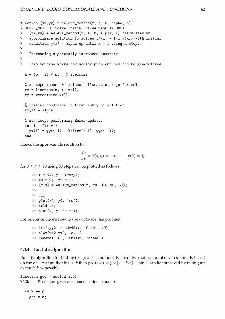
CHAPTER 4. LOOPS, CONDITIONALS AND FUNCTIONS 42
function [xx,yy] = eulers_method(f, a, b, alpha, n)
%EULERS_METHOD Solve initial value problem ODEs
% [xx,yy] = eulers_method(f, a, b, alpha, n) calculates an
% approximate solution to solves y'(x) = f(x,y(x)) with initial
% condition y(a) = alpha up until x = b using n steps.
%
% Increasing n generally increases accuracy.
%
% This version works for scalar problems but can be generalized.
h = (b - a) / n; % stepsize
% n steps means n+1 values, allocate storage for soln
xx = linspace(a, b, n+1);
yy = zeros(size(xx));
% initial condition is first entry of solution
yy(1) = alpha;
% now loop, performing Euler updates
for i = 2:(n+1)
yy(i) = yy(i-1) + h*f(xx(i-1), yy(i-1));
end
Hence the approximate solution to
dydx
= f (x, y) = −xy, y(0) = 1,
for 0 ≤ x ≤ 10 using 50 steps can be plotted as follows:
>> f = @(x,y) (-x*y);
>> x0 = 0; y0 = 1;
>> [x,y] = eulers_method(f, x0, 10, y0, 50);
>>
>> clf
>> plot(x0, y0, 'ro');
>> hold on;
>> plot(x, y, 'k.-');
For reference, here’s how to use ode45 for this problem:
>> [xx2,yy2] = ode45(f, [0 10], y0);
>> plot(xx2,yy2, 'g.-')
>> legend('IC', 'Euler', 'ode45')
4.4.4 Euclid’s algorithm
Euclid’s algorithm for finding the greatest common divisor of two natural numbers is essentially basedon the observation that if a > b then gcd(a, b) = gcd(a− b, b). Things can be improved by taking offas much b as possible:
function gcd = euclid(a,b)
%GCD Find the greatest common denominator
if b == 0
gcd = a;
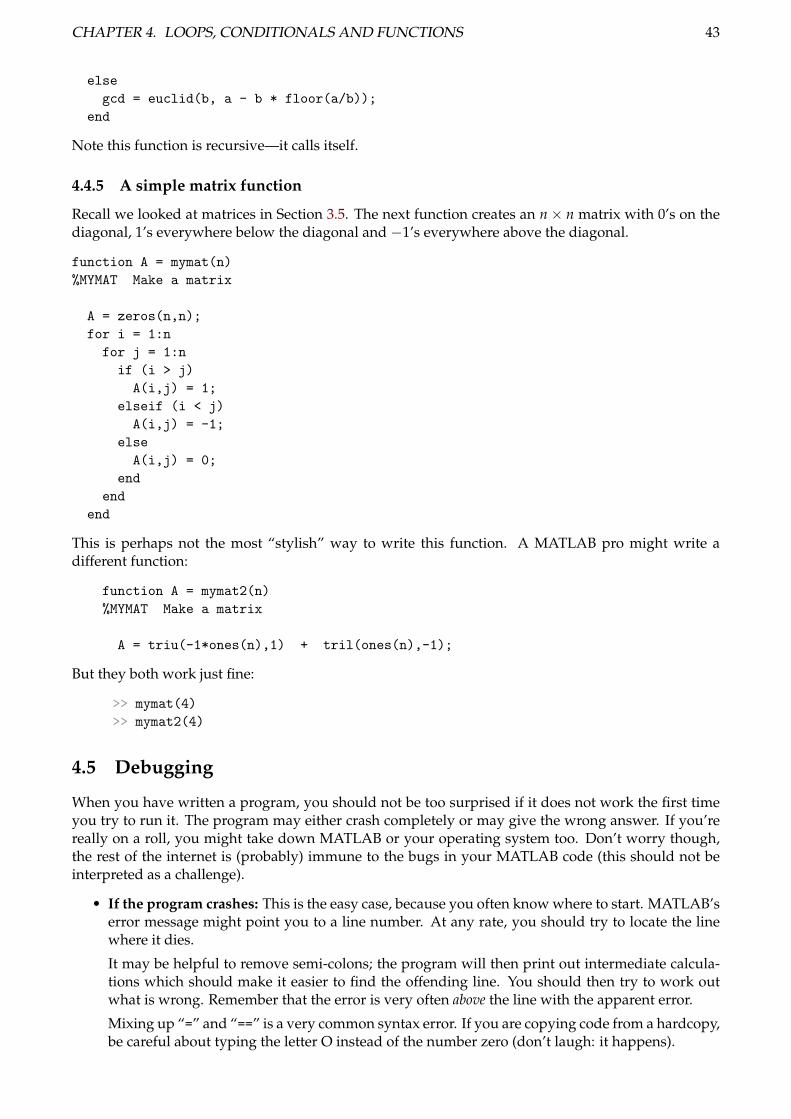
CHAPTER 4. LOOPS, CONDITIONALS AND FUNCTIONS 43
else
gcd = euclid(b, a - b * floor(a/b));
end
Note this function is recursive—it calls itself.
4.4.5 A simple matrix function
Recall we looked at matrices in Section 3.5. The next function creates an n× n matrix with 0’s on thediagonal, 1’s everywhere below the diagonal and −1’s everywhere above the diagonal.
function A = mymat(n)
%MYMAT Make a matrix
A = zeros(n,n);
for i = 1:n
for j = 1:n
if (i > j)
A(i,j) = 1;
elseif (i < j)
A(i,j) = -1;
else
A(i,j) = 0;
end
end
end
This is perhaps not the most “stylish” way to write this function. A MATLAB pro might write adifferent function:
function A = mymat2(n)
%MYMAT Make a matrix
A = triu(-1*ones(n),1) + tril(ones(n),-1);
But they both work just fine:
>> mymat(4)
>> mymat2(4)
4.5 Debugging
When you have written a program, you should not be too surprised if it does not work the first timeyou try to run it. The program may either crash completely or may give the wrong answer. If you’rereally on a roll, you might take down MATLAB or your operating system too. Don’t worry though,the rest of the internet is (probably) immune to the bugs in your MATLAB code (this should not beinterpreted as a challenge).
• If the program crashes: This is the easy case, because you often know where to start. MATLAB’serror message might point you to a line number. At any rate, you should try to locate the linewhere it dies.
It may be helpful to remove semi-colons; the program will then print out intermediate calcula-tions which should make it easier to find the offending line. You should then try to work outwhat is wrong. Remember that the error is very often above the line with the apparent error.
Mixing up “=” and “==” is a very common syntax error. If you are copying code from a hardcopy,be careful about typing the letter O instead of the number zero (don’t laugh: it happens).
CHAPTER 4. LOOPS, CONDITIONALS AND FUNCTIONS 44
• If the program runs but gives the wrong answer: This is the harder case; it may prove quitedifficult to locate and correct the error. The first thing is to convince yourself that your programis trying to solve the right problem. You should try to run the program for very simple cases,and find the simplest case in which it gives the wrong answer. Remove all code that is notused in that particular calculation. This is relatively easy to do by inserting % to make them intocomments.
If you have written functions, test them separately to make sure they behave as you expect.
Add some “debugging output” by removing semi-colons or otherwise printing out intermediateresults. Trace this output manually to find a point where the results don’t match what youexpect.
• Watch out for floating point when you were expected symbolic results (and vice versa). “whos”is your friend.
• The MATLAB graphical user interface provides various features to help you debug code such asbreakpoints. The command “keyboard” is useful for debugging functions: add this commandto your function and when MATLAB gets there, it gives you access on the command line to thevariables inside you function.
4.6 Further exercise
The following is a final optional exercise on functions.
Exercise 4.7 Write a function that displays the rows of Pascal’s triangle up to and including the nthrow for a given positive integer n. �
Appendix A
Simplification
A key strength of computer algebra systems like the Symbolic Math Toolbox is the ability to manip-ulate mathematical expressions symbolically. The symbolic manipulation of expressions occasionally(on a bad day you might say “often”) creates results in a different form than what the user needs. Itis thus useful to know how to persuade the toolbox to change the form of a particular expression intowhat is needed. This is more of an art than a science but experience and a working knowledge of thecommands and techniques introduced here can be helpful.
A.1 Expand
The expand command does exactly what its name implies. In this section we will look at how itworks when applied to polynomials and to trigonometric functions. For example the expansion of(x + 1)(x + z)2 is found by typing
>> syms x y z
>> expand((x+1)*(x+z)^2)
>> pretty(ans)
When applied to trigonometric functions expand uses the sum rules1 to remove multiple angles, re-placing them with powers:
>> expand(cos(2*x))
(remember that in the output cos(x)^2 means cos2 x, etc.) Other examples of the expand commandare
>> expand(sin(x+y))
>> expand(cos(2*x+y))
>> expand(cos(5*x))
>> pretty(ans)
Perhaps in the last example above we wished instead to obtain the partial expansion cos 5x = cos 4x cos x−sin 4x sin x; we could use a little trickery:
>> c = expand(cos(x+y))
>> c2 = subs(c, y, 4*x)
Hyperbolic expressions can be expanded in much the same manner; for example try
>> expand(sinh(3*x))
1cos(x± y) = cos x cos y∓ sin x sin y is an example of a sum rule.
45
APPENDIX A. SIMPLIFICATION 46
A.2 Factor
For polynomials the factor command is in some ways the opposite of expand, and often does as onewould expect:
>> syms x y z
>> factor(x^5 - x^4 - 7*x^3 + x^2 + 6*x)
>> f = x^4 + 4*x^3*y - 7*x^2*y^2 - 22*x*y^3 + 24*y^4
>> factor(f)
In the second example above f has been defined first; this is a useful trick with long expressions tocheck that they are typed correctly before proceeding. The factor command can also be used onrational expressions:
>> g = factor( (x^3 - y^3) / (x^4 - y^4) )
>> pretty(g)
(where the common factor (x− y) in the numerator and denominator has been cancelled).
Exercise 5.1 Expand the function f = (x + y + 1)3 and then factorise f − 1. �
Exercise 5.2 Use MATLAB to show thatn
∑r=1
r =12
n(n + 1),
n
∑r=1
r2 =16
n(n + 1)(2n + 1),
n
∑r=1
r3 =14
n2(n + 1)2.
(You might want to review Section 3.4.3.) �
A.3 Collect
The command collect is useful when you want to collect terms in powers of a known expression.
>> syms x
>> g = (cos(x) + 1)*(cos(x) + 2)*(cos(x) + 3)
>> collect(g, cos(x))
A.4 Simplify
The command simplify() is the most general of the Symbolic Math Toolbox’s simplification com-mands and is usually the one to be tried first. However, it is not always the most appropriate com-mand and results can be unpredictable.
Positive integer powers of trigonometric and hyperbolic functions are simplified by this rule as faras possible, as illustrated by the following attempt to simplify sinh4 x− cosh4 x:
>> syms x y z
>> f = (sinh(x))^4 - (cosh(x))^4
>> simplify(f)
One of the most useful applications of simplify or simple is when trying to verify that expr == expr2,where expr1 and expr2 are both expressions. Here is example, an attempt to verify that
1 + tanh2 x1− tanh2 x
= cosh 2x :
APPENDIX A. SIMPLIFICATION 47
>> expr1 = (1+tanh(x)^2) / (1-tanh(x)^2);
>> expr2 = cosh(2*x);
>> simplify(expr1 - expr2)
The following exercises will give you some practice using the simplify command and also someearlier commands.
Exercise 5.3 Use simplify to show that
if y =1 + sin x1 + cos x
thendydx
=cos x + sin x + 1
1 + 2 cos x + cos2 x;
if y = ln
√1 + x1− x
thendydx
= − 1−1 + x2 ;
if y = ln((1 + x)1/2
(1− x)1/3
)then
dydx
=−5 + x
6(−1 + x2).
�
Exercise 5.4 Consider the general cubic polynomial
f (x) =13
ax3 + bx2 + cx + d,
where a, b, c and d are real constants. If the stationary points of f are at x1 and x2, use MATLAB toshow that
f (x1)− f (x2) = −a6(x1 − x2)
3.
�
Exercise 5.5 Show that the function f = 1/r, where r2 = (x− a)2 + (y− b)2 + (z− c)2 and a, b and care constants, is a solution of Laplace’s equation
∂2 f∂x2 +
∂2 f∂y2 +
∂2 f∂z2 = 0.
�
Appendix B
Other advanced topics
B.1 MATLAB “handle” functions and anonymous functions
We have seen that functions can be created using .m files (Section 4.3). You can create function handlesusing “anonymous functions”. This is most helpful for making a short function, for example:
>> alpha = 0.5
>> y = @(x) sin(alpha*x)
>> y(pi)
You can also create these sorts of functions from symbolic expressions:
>> syms x
>> y = sin(x)
>> ym = matlabFunction(y)
See help function_handle and help matlabFunction for more information.
B.2 Variable precision arithmetic
“Out-of-the-box” MATLAB focuses on supporting double precision floating point (the double class).Recall this class represents numbers using a precision of roughly 15 decimal digits. The SymbolicMath Toolbox (based on MuPAD) adds support for symbolic expressions (using the sym and symfun
classes). The Symbolic Math Toolbox also adds support for Variable Precision Arithmetic via the vpa
class. Having floating point numbers with more than 15 digits can be a useful feature and so thischapter is essentially for your own interest or reference.
To use variable precision arithmetic, first set the desired precision. Then use vpa() or a quotedsymbolic constructor with a decimal place.
>> digits(64)
>> a = vpa(2/3)
>> b = sym('2.0')/3
Note that b = sym(2.0)/3 won’t work (why not?). Probably the vpa() command is less prone toaccidental unwanted use.
It is worth noting that the clear command does not reset digits to its default value. But clear all
will.
Exercise 6.1 All rational numbers p/q, where p and q are integers (q 6= 0), have a terminating or(eventually) repeating decimal form. By increasing the precision using digits() as appropriate, findthe exact decimal form of 21/23. �
48
APPENDIX B. OTHER ADVANCED TOPICS 49
Exercise 6.2 The following two expressions are both approximations to π that were discovered by theIndian mathematician Ramanujan (1887–1920):
π1 =12√190
ln((2√
2 +√
10)(3 +√
10))
and
π2 =
√√92 +
192
22.
Use VPA to find the absolute errors |π1 − π| and |π2 − π|. Hence determine how good these approxi-mations actually are. �
B.3 Cell Arrays
Recall that a vector in MATLAB is homogeneous: everything inside it must be the same type (double,sym, etc). How dull! Cell arrays on the other hand can store anything, even other cell arrays. Makeone like this:
>> A = {'Freedom!', sym(2/3), rand(3,3)}>> A{1}>> A{2}>> A{3}
A common use of cell arrays is to store a “list of strings”. This is because an array of strings justconcatenates them. For example:
>> L = ['red' 'lorry' 'yellow' 'lorry']
>> % output is 'redlorryyellowlorry'
>> S = {'red' 'lorry' 'yellow' 'lorry'}>> % output is a 4-element cell array
This is useful for constructing legends for plots when using loops.
Academic Honesty
In Michaelmas Term you are encouraged to co-operate with fellow students in learning to use thesystem and to use MATLAB. The Hilary Term projects, however, must be your own unaided work.
The description of each project gives references to books covering the relevant mathematics. If youcannot understand some of this then you are free to consult your tutors or others about it, but notabout the project itself. You may discuss with the demonstrators and others the techniques describedin the Michaelmas Term Student Guide, and the commands listed in the Hilary Term Student Guideor found in the MATLAB Help pages. You may ask the course director to clarify any obscure pointsin the projects.
The projects must be your own unaided work. You will be asked to make a declaration to thateffect when you submit them.
University ICT Regulations
All use of the computing and network facilities in the Oxford University Computing Services, as wellas all other computing and network facilities throughout the University of Oxford and associated Col-leges, is subject to certain rules. These rules concern what is considered to be unacceptable behaviourand misuse, as well as what may infringe licence terms or may be otherwise illegal. Note that all use ispermitted for bona fide purposes only, and is subject to proper authorization (which may be providedeither explicitly or implicitly).
The University regards computer misuse as a serious matter which may warrant disciplinary (or evencriminal) proceedings.
The rules by which you have agreed to be bound can be found at the following webpages:
http://www.admin.ox.ac.uk/statutes/regulations/196-052.shtml
https://www.maths.ox.ac.uk/members/it/it-notices-policies
50