Embed Size (px)
Citation preview
Mathematical Methods forValuation and Risk Assessment of
Investment Projects and RealOptions
Myriam Cisneros-Molina
Oriel College
University of Oxford
A thesis submitted for the degree of
Doctor of Philosophy
Trinity 2006

I wish to express my gratitude to my supervisor Dr. Sam D. Howison for his
patience and multiple fruitful conversations. To the Oxford Centre for Industrial and
Applied Mathematics, the Mathematical Institute and Oriel College for providing me
with the right atmosphere to work through my PhD.
I want to thank my family for believing in me, their unconditional support and
love even in the distance and difficulties. I am specially grateful to my husband for
all his strong support and encouragement over the years.
Financial support by The Mexican Science and Technology Council (CONACYT)
and the Mexican Petroleum Institute (IMP) is gratefully acknowledged.
Abstract
In this thesis, we study the problems of risk measurement, valuation and
hedging of financial positions in incomplete markets when an insufficient
number of assets are available for investment (real options). We work
closely with three measures of risk: Worst-Case Scenario (WCS) (the
supremum of expected values over a set of given probability measures),
Value-at-Risk (VaR) and Average Value-at-Risk (AVaR), and analyse the
problem of hedging derivative securities depending on a non-traded asset,
defined in terms of the risk measures via their acceptance sets. The hedg-
ing problem associated to VaR is the problem of minimising the expected
shortfall. For WCS, the hedging problem turns out to be a robust version
of minimising the expected shortfall; and as AVaR can be seen as a partic-
ular case of WCS, its hedging problem is also related to the minimisation
of expected shortfall.
Under some sufficient conditions, we solve explicitly the minimal expected
shortfall problem in a discrete-time setting of two assets driven by corre-
lated binomial models.
In the continuous-time case, we analyse the problem of measuring risk
by WCS, VaR and AVaR on positions modelled as Markov diffusion pro-
cesses and develop some results on transformations of Markov processes
to apply to the risk measurement of derivative securities. In all cases,
we characterise the risk of a position as the solution of a partial differ-
ential equation of second order with boundary conditions. In relation
to the valuation and hedging of derivative securities, and in the search
for explicit solutions, we analyse a variant of the robust version of the
expected shortfall hedging problem. Instead of taking the loss function
l(x) = [x]+ we work with the strictly increasing, strictly convex function
Lε(x) = ε log
(1+exp−x
εexp−x
ε
). Clearly limε→0 Lε(x) = l(x). The reformula-
tion to the problem for Lε(x) also allow us to use directly the dual theory
under robust preferences recently developed in [82]. Due to the fact that

the function Lε(x) is not separable in its variables, we are not able to
solve explicitly, but instead, we use a power series approximation in the
dual variables. It turns out that the approximated solution corresponds
to the robust version of a utility maximisation problem with exponential
preferences (U(x) = − 1γe−γx) for a preferences parameter γ = 1
ε. For the
approximated problem, we analyse the cases with and without random
endowment, and obtain an expression for the utility indifference bid price
of a derivative security which depends only on the non-traded asset.
Mathematical Methods for Valuation and Risk
Assessment of Investment Projects and Real
Options
Myriam Cisneros-Molina
Oriel CollegeUniversity of Oxford
A thesis submitted for the degree ofDoctor of Philosophy
Trinity 2006
In this thesis, we study the problems of risk measurement, valuation and hedging of
financial positions in incomplete markets when an insufficient number of assets are
available for investment (real options). We work closely with three measures of risk:
Worst-Case Scenario (WCS) (the supremum of expected values over a set of given
probability measures), Value-at-Risk (VaR) and Average Value-at-Risk (AVaR), and
analyse the problem of hedging derivative securities depending on a non-traded asset,
defined in terms of the risk measures via their acceptance sets. The hedging problem
associated to VaR is the problem of minimising the expected shortfall. For WCS,
the hedging problem turns out to be a robust version of minimising the expected
shortfall; and as AVaR can be seen as a particular case of WCS, its hedging problem
is also related to the minimisation of expected shortfall.
Under some sufficient conditions, we solve explicitly the minimal expected shortfall
problem in a discrete-time setting of two assets driven by correlated binomial models.
In the continuous-time case, we analyse the problem of measuring risk by WCS,
VaR and AVaR on positions modelled as Markov diffusion processes and develop some
results on transformations of Markov processes to apply to the risk measurement
of derivative securities. In all cases, we characterise the risk of a position as the
solution of a partial differential equation of second order with boundary conditions.
In relation to the valuation and hedging of derivative securities, and in the search for
explicit solutions, we analyse a variant of the robust version of the expected shortfall
hedging problem. Instead of taking the loss function l(x) = [x]+ we work with
the strictly increasing, strictly convex function Lε(x) = ε log
(1+exp−x
εexp−x
ε
). Clearly
limε→0 Lε(x) = l(x). The reformulation to the problem for Lε(x) also allow us to use
directly the dual theory under robust preferences recently developed in [82]. Due to
the fact that the function Lε(x) is not separable in its variables, we are not able to
solve explicitly, but instead, we use a power series approximation in the dual variables.

It turns out that the approximated solution corresponds to the robust version of
a utility maximisation problem with exponential preferences (U(x) = − 1γe−γx) for
a preferences parameter γ = 1ε. For the approximated problem, we analyse the
cases with and without random endowment, and obtain an expression for the utility
indifference bid price of a derivative security which depends only on the non-traded
asset.
Contents
Introduction i
1 Preliminaries 7
1.1 Introduction . . . . . . . . . . . . . . . . . . . . . . . . . . . . . . . . 7
1.2 Risk factors and exposure to uncertainty in risk assessment . . . . . . 8
1.3 Static risk measures . . . . . . . . . . . . . . . . . . . . . . . . . . . . 10
1.3.1 Acceptance sets and risk measures . . . . . . . . . . . . . . . 13
1.3.2 Robust representation of convex risk measures . . . . . . . . . 16
1.4 Dynamic risk measures . . . . . . . . . . . . . . . . . . . . . . . . . . 17
1.5 The risk measures: WCS, VaR and AVaR . . . . . . . . . . . . . . . . 18
1.5.1 Worst-Case-Scenario . . . . . . . . . . . . . . . . . . . . . . . 18
1.5.1.1 The hedging problem . . . . . . . . . . . . . . . . . . 20
1.5.2 Value-at-Risk . . . . . . . . . . . . . . . . . . . . . . . . . . . 23
1.5.2.1 The hedging problem . . . . . . . . . . . . . . . . . . 25
1.5.3 Average Value-at-Risk . . . . . . . . . . . . . . . . . . . . . . 26
1.5.3.1 The hedging problem . . . . . . . . . . . . . . . . . . 29
1.6 Superreplication and partial hedging . . . . . . . . . . . . . . . . . . 29
I Risk and Hedging in Discrete-time: A Two-factor Bino-mial Model 33
2 Minimisation of Expected Shortfall 34
2.1 Introduction . . . . . . . . . . . . . . . . . . . . . . . . . . . . . . . . 34
2.2 The two-step procedure in the minimisation of expected shortfall . . 35
2.3 The two-factors N-period binomial model for the expected shortfall . 37
2.3.1 Marginal martingale measures . . . . . . . . . . . . . . . . . . 39
2.3.2 Some important martingale measures . . . . . . . . . . . . . . 40
2.3.2.1 The impact measures . . . . . . . . . . . . . . . . . . 40
i
2.3.2.2 The upper and lower bound measures . . . . . . . . 41
2.3.3 Minimising the expected shortfall . . . . . . . . . . . . . . . . 44
2.3.4 Relation with the two-step procedure . . . . . . . . . . . . . . 45
2.3.5 The single-period model . . . . . . . . . . . . . . . . . . . . . 46
2.3.5.1 The strategies, the impact and the extreme measures 46
2.3.5.2 The three initial capital cases . . . . . . . . . . . . . 51
2.3.6 The large capital case for the N-period model . . . . . . . . . 58
2.3.6.1 Interpretation of the optimal expected shortfall . . . 59
2.3.6.2 Analysis of the strategies . . . . . . . . . . . . . . . 61
2.3.6.3 The initial capital condition . . . . . . . . . . . . . . 62
2.3.6.4 The large capital case and the two-step procedure . . 65
2.3.6.5 Numerical example . . . . . . . . . . . . . . . . . . . 67
2.3.7 The discrete-time as an approximation to a continuous time
model . . . . . . . . . . . . . . . . . . . . . . . . . . . . . . . 69
2.3.7.1 Numerical example . . . . . . . . . . . . . . . . . . . 74
II Risk and Hedging in Continuous-time: Ito DiffusionModels 80
3 WCS, VaR and AVaR 81
3.1 Introduction . . . . . . . . . . . . . . . . . . . . . . . . . . . . . . . . 81
3.2 The model . . . . . . . . . . . . . . . . . . . . . . . . . . . . . . . . . 82
3.3 Worst Conditional Scenario risk measure (WCS) . . . . . . . . . . . . 83
3.3.1 Change of measure . . . . . . . . . . . . . . . . . . . . . . . . 84
3.3.2 Change of measure that preserves the Markov property . . . . 85
3.3.2.1 Exponential change of measure for Markov processes 85
3.3.3 Finding an exponential change of measure that gives a specific
homogeneous drift . . . . . . . . . . . . . . . . . . . . . . . . 90
3.3.4 WCS under Markovian priors . . . . . . . . . . . . . . . . . . 91
3.3.5 WCS as a stochastic control problem . . . . . . . . . . . . . . 97
3.4 Value-at-Risk (VaR) . . . . . . . . . . . . . . . . . . . . . . . . . . . 99
3.5 Average Value-at-Risk (AVaR) . . . . . . . . . . . . . . . . . . . . . . 100
3.6 Computation of risk measures when the transition density is known . 101
3.6.1 WCS . . . . . . . . . . . . . . . . . . . . . . . . . . . . . . . . 101
3.6.2 VaR . . . . . . . . . . . . . . . . . . . . . . . . . . . . . . . . 104
3.6.3 AVaR . . . . . . . . . . . . . . . . . . . . . . . . . . . . . . . 105
ii
3.6.4 Example of risk measures for a single process . . . . . . . . . . 106
4 Risk for Derivatives 111
4.1 Introduction . . . . . . . . . . . . . . . . . . . . . . . . . . . . . . . . 111
4.2 Risk measures for European derivatives . . . . . . . . . . . . . . . . . 112
4.2.1 The derivative-dynamics . . . . . . . . . . . . . . . . . . . . . 112
4.2.2 Homogeneous local transformations . . . . . . . . . . . . . . . 113
4.2.3 The process C(t, St) as a local transformation of the St process 118
4.2.3.1 Injective local transformations . . . . . . . . . . . . . 118
4.2.3.2 Piecewise injective transformations . . . . . . . . . . 121
4.2.4 Example . . . . . . . . . . . . . . . . . . . . . . . . . . . . . . 129
4.3 Relation to the delta and delta-gamma approaches for risk of derivatives142
4.3.1 The delta-approach . . . . . . . . . . . . . . . . . . . . . . . . 142
4.3.2 The delta-gamma approach . . . . . . . . . . . . . . . . . . . 143
4.4 Risk measures for American derivatives . . . . . . . . . . . . . . . . . 144
5 Hedging and Derivative Pricing in the Robust ε-expected Shortfall
Problem 145
5.1 Introduction . . . . . . . . . . . . . . . . . . . . . . . . . . . . . . . . 145
5.2 The financial model . . . . . . . . . . . . . . . . . . . . . . . . . . . . 146
5.3 The wealth process . . . . . . . . . . . . . . . . . . . . . . . . . . . . 147
5.4 Equivalent measures . . . . . . . . . . . . . . . . . . . . . . . . . . . 148
5.4.1 Local martingale measures . . . . . . . . . . . . . . . . . . . . 148
5.4.2 The minimal martingale measure . . . . . . . . . . . . . . . . 149
5.5 The set of priors P . . . . . . . . . . . . . . . . . . . . . . . . . . . . 149
5.6 The robust ε-expected shortfall hedging problem . . . . . . . . . . . . 150
5.6.1 Reformulation of the problem . . . . . . . . . . . . . . . . . . 151
5.6.2 Utility indifference pricing for the robust ε-ES hedging problem 152
5.6.3 Maximising utility with no random endowment . . . . . . . . 153
5.6.3.1 Optimal Lagrange multiplier . . . . . . . . . . . . . . 157
5.6.3.2 An approximation to the dual and primal value func-
tions . . . . . . . . . . . . . . . . . . . . . . . . . . . 161
5.6.3.3 The solution to the dual problem . . . . . . . . . . . 163
5.6.3.4 Approximation to the optimal strategy . . . . . . . . 165
5.6.4 Maximising utility with random endowment . . . . . . . . . . 167
5.6.4.1 The problem (P2b) . . . . . . . . . . . . . . . . . . . 169
5.6.4.2 The problem (P2a) . . . . . . . . . . . . . . . . . . . 175
iii
5.7 Utility indifference pricing for the approximated problems . . . . . . . 178
5.8 Conclusions . . . . . . . . . . . . . . . . . . . . . . . . . . . . . . . . 179
6 Future Research 180
A Some Important Examples of Risk Measures 182
A.1 Shortfall risk measures . . . . . . . . . . . . . . . . . . . . . . . . . . 182
A.1.1 The hedging problem . . . . . . . . . . . . . . . . . . . . . . . 183
A.1.2 Robust representation of shortfall risk measures . . . . . . . . 184
A.2 State-dependent utility functions derived from shortfall risk measures 188
A.2.1 Examples of loss functions, their corresponding utility functions
and Fenchel-Legendre transforms . . . . . . . . . . . . . . . . 188
B Duality Theory for Optimal Investment Problems on Semimartin-
gales 189
B.1 The model . . . . . . . . . . . . . . . . . . . . . . . . . . . . . . . . . 189
B.2 The single prior case . . . . . . . . . . . . . . . . . . . . . . . . . . . 190
B.2.1 The primal problem . . . . . . . . . . . . . . . . . . . . . . . 190
B.2.2 The dual problem . . . . . . . . . . . . . . . . . . . . . . . . . 191
B.2.3 Relation between the primal and dual problem . . . . . . . . . 191
B.3 The robust utility maximisation case . . . . . . . . . . . . . . . . . . 193
B.3.1 The multiple priors primal problem . . . . . . . . . . . . . . . 194
B.3.2 The multiple priors dual problem . . . . . . . . . . . . . . . . 195
B.3.3 Relation between the primal and dual problem . . . . . . . . . 195
B.4 Proof of Lemma 107 . . . . . . . . . . . . . . . . . . . . . . . . . . . 197
C Selecting a Measurable Function 198
D Some Results Related with sup and inf of Sets and Functions 199
Bibliography 201
iv
Introduction
With the dissemination of quantitative methods in the financial sector and advent
of complex derivative products, mathematical models have come to play an increas-
ingly important role in financial decision making, especially in the context of pricing,
hedging and risk management of derivative instruments.
In view of the recent treatment of the quantification of risk (initiated in [3] and
further developed in [16], [29], and [35]; see also [32]) based on a set of desired axioms
that every risk measure should satisfy, defining in such a way the class of coherent and
convex risk measures, the “fair”pricing of derivative securities or risk-neutral valuation
becomes a particular case of measuring risk under an arbitrage-free condition.
The other aspect inherent in measuring risk is the hedging of financial securities.
Hedging and measuring risk are two faces of one procedure, as the same three elements
to defining risk: a system of prices, a class of permitted actions and a criterion of
acceptability are needed for both of them.
It is a well known fact that pricing and hedging of a given contingent claim has
a unique solution in a complete market framework, but when some incompleteness
is introduced the problem becomes more difficult and an extra criterion is needed in
order to pick one price between all arbitrage-free prices.
One alternative method of valuation and hedging in incomplete markets is to use
a “superhedging strategy”(see [20] and [52]). But from a practical point of view the
cost of superhedging is often too high. Also perfect (super-) hedging takes away
the opportunity of making a profit together with the risk of a loss. Suppose the
investor is unwilling to put up the initial amount of capital required for a superhedge
and is ready to accept some risk. Another set of criteria to pricing and hedging in
incomplete markets is called utility maximisation, and it is perhaps, one of the most
popular ones. Proposed by Hodges and Neuberger (1989), the price of the contingent
claim is obtained as the smallest (resp. largest) amount leading the agent indifferent
between selling (resp. buying) the claim and doing nothing. The price obtained is the
indifference seller’s (resp. buyer’s) price. Typically the utility function is assumed to
1
be a strictly increasing and strictly concave function on the real line, but ideas can
be extended to the cases when the utility function is just increasing and concave and
maybe state dependent. Examples of criteria like these are what are called: expected
shortfall, and maximising the probability of a perfect hedge.
Although most of the criteria above for pricing and hedging of financial securities
were initially formulated in a specific context, all of them can be reinterpreted as
measuring risk (valuation) and finding the hedging strategy for a corresponding risk
measure. This point of view is adopted in the present thesis.
Organisation of the thesis and contributions
In this thesis, we study the problems of risk measurement, valuation and hedging
of financial positions in incomplete markets when insufficient number of assets are
available for complete hedging. One application is to real options.
Chapter 1 contains some background material needed throughout the thesis. The
first part discusses the axiomatic approach of risk measures introduced in [3] and
further developed in [16], [29] and [30]. We then define the three main measures of risk
analysed throughout the thesis, namely: Worst-Case-Scenario risk measure (WCS)
(the supremum of the expected values over a set of given probability measures), Value-
at-Risk (VaR), and Average value-at-Risk (AVaR). We conclude Chapter 1 with the
connection between measuring risk and the associated hedging problems (defining
acceptability of the positions via the risk measure).
Before describing the rest of the thesis, we briefly set the mathematical scene (the
practical applications will be described later). Assume we work in a complete filtered
probability space (Ω,F , (F)0≤t≤T , P), and that an investor faces a random liability
H ≥ 0 at time T . If the market is complete and free of arbitrage opportunities,
under mild conditions, any contingent claim H with fixed payoff at time T can be
replicated or hedged by a trading strategy (v, π) consisting of an initial capital v ≥ 0
and a dynamic portfolio process π ∈ A(v)1. When the market is not complete, then
the existence of a replicating process (v, π) cannot always be guaranteed, unless the
investor is prepared to hold an initial capital equal to the super-replicating price
supQ∈Me
EQ [HT ] ,
where Me denotes the set of all equivalent martingale measures with respect to the
probability P. In this case, the risk involved in the payment H can be completely
1A(v) denotes the set of admissible portfolios. It will be defined in detail in the later chapters.
2
eliminated because a super-hedging strategy can be performed. On the other hand,
when the investor is only willing to put up a smaller amount of the initial capital
v ∈(
0, supQ∈Me
EQ [HT ]
),
then a non-hedgeable risk will be involved and any hedging strategy (v, π) will be
“partial” in the sense that its shortfall
(HT − VT )+
may be non-zero with positive probability, where VT denotes the value at time T
of the wealth associated to the replicating strategy (v, π). This situation induces
the so-called shortfall risk minimisation problem: For a fixed initial capital v ∈(0, sup
Q∈Me
EQ [HT ]
), find a trading strategy (v, π), with v ≤ v and π ∈ A(v) such that
the expected shortfall
EP[(HT − VT )+
]is minimal under the physical probability measure P.
This problem has been studied in the context of semimartingale processes and
general Ito diffusions (see [9], [28] and [31, p. 341]) in the sense that the authors have
shown existence and general characterisation of the solution (the trading strategy
and the minimal expected shortfall). It turns out that the solution to the minimal
expected shortfall problem can be divided into two parts: The first is the solution to
a “static-hedging” problem, of minimising
EP[(HT − Y )+
]among all FT -measurable random variables Y ≥ 0 which satisfy the constraint
supQ∈Me
EQ [Y ] ≤ v.
If Y ∗ denotes the solution in the first part, then the second part consists of fitting the
terminal value VT of an admissible strategy to the optimal solution Y ∗. Although it
has been shown that the solution exists and is characterised via the above two-step
procedure, few explicit solutions or approximating algorithms have been studied in
the literature. They will rely of course on the particular model assumed. In relation
to the discrete-time settings, [23] has studied the problem with a single asset under
binomial dynamics with model uncertainty leading to an incomplete-market situation;
[79] provides an algorithm for the trinomial model of one asset, and [83] presents some
3
general results for the multi-state case for a single risky asset. The multi-assets case
in a complete financial market has been solved in [79].
As our interest is in real options situations (when the incompleteness of the market
comes from insufficient number of assets available for investment), in Chapter 2 we
analyse the problem of minimising the expected shortfall of a random liability faced at
a fixed future time T in an incomplete market consisting of one riskless asset and two
risky assets S and Y , but only one of them (S) is tradable in the market. We model
S and Y in discrete-time as two correlated N -period binomial trees, and assume that
the liability payoff at time T is a function only on the non traded asset of the form
H(YT ). This setting can be seen as the simpler Markov-chain approximation to its
continuous-time counterpart. Using dynamic programming techniques, we are able
to find explicitly the minimal expected shortfall and the optimal strategy that solve
the problem under a set of sufficient conditions. In the general case, we find upper
and lower bounds for the minimal shortfall.
In the second part of the thesis, we focus on continuous-time models. We start
Chapter 3 by computing the three measures of risk of interest (WCS, VaR and AVaR)
for positions whose models are given by continuous Markov diffusion processes. The
main idea to compute risk given by VaR or AVaR of a position X modelled as a
diffusion process is to exploit the Markov property and characterise it as the solution
to a second-order partial differential equation (PDE) with boundary conditions. In
the case of the WCS risk measure, the approach is similar but less direct, as the WCS
is defined as the supremum over a set of probability measures. In order to obtain
WCS also as the solution to a boundary value PDE we need to state conditions on
the set of measures, so the supremum in the definition of WCS is finite.
Motivated by practical application, firstly, we analyse in detail the case when under
each measure on the definition of WCS the process X remains a Markov diffusion
process. This involves the study of properties of what is called an exponential change
of measure transformation of Markov processes and to adapt some results to our
present situation. In most of the cases, the PDEs that characterise the risk measures
do not have explicit solutions and series expansion or numerical methods need to be
applied. In the few cases that do allow explicit solution, solving for the risk PDEs or
solving for the transition probability density of the process X are equivalent. This is
shown in the last part of Chapter 3.
When the restriction on the Markov property is lifted, we establish conditions so
the computation of WCS can be formulated as a stochastic control problem and then
4
as the solution to a nonlinear PDE of second order with boundary condition and a
terminal condition. We end the chapter with several examples.
In Chapter 4 we study the problem of computing risk as WCS, VaR and AVaR for
derivative securities that depend on an underlying asset given by a Markov diffusion
processes as in the preceding chapter. This is, we assume that the derivative security
is defined by a positive payoff function H(ST ) on the final value of a security St.
By the Markov property and our assumptions on the process St the random variable
H(ST ) may be written as a function C ∈ C1,2 on the process St at the current time
t. Defining a process given by
Xt = C(t, St),
one can apply Ito’s lemma to obtain the dynamics of X. Then our problem reduces
to the one studied in the previous chapter of computing the risk for the position X.
When the function C is not injective, the dynamics of the process Xt may be degen-
erate. In order to analyse this situation in detail, we look at the process Xt from the
point of view of a local transformation of the process St. In particular, we establish
conditions and analyse when the transition probability density of a transformed pro-
cess X can be expressed in terms of the transition probability density of our original
process S. In other words, we find how to reduce the solution to the risk-PDEs for
the position X to the solution of simpler PDEs corresponding to the solution to the
risk-PDEs for the position S.
We apply our results on local transformation of Markov diffusion processes to the
computation of risk for derivative securities and illustrate them with examples. We
discuss briefly also the relation to this method with the approaches known as delta-
and delta-gamma approximation for the computation of risk of derivatives.
Concerning the hedging problems corresponding to the WCS, VaR and AVaR, in
Chapter 5 we analyse a variant of the robust version of the expected shortfall hedging
problem:
For an initial capital x ≥ 0, find a hedging strategy (x, π), π ∈ A(x) with terminal
value X(x,π)T which optimises
infπ∈A(x)
supQ∈P
EQ
[(HT −X
(x,π)T
)+], (1)
in a continuous-time model consisting of two risky assets St and Yt, 0 ≤ t ≤ T (given
by geometric Brownian motion) and a risk-free bond Bt, 0 ≤ t ≤ T . The asset St is
assumed to be traded in the financial market but Yt is not traded.
5
We consider a random payoff HT to be function of the underlying process Yt at
time T , that is, HT = H(YT ) and the set of measures (priors) P to be a subset of the
equivalent probability measures Me.
The problem in (1) corresponds to the hedging problem for the WCSP risk measure
discussed in Chapter 1 Section 1.5.1.1. For the particular choice of priors P = Pand2 P = Q ∈ Ma : dQ
dP is P-a.s. bounded by 1α introduced in Proposition 30, we
recover the solution to the hedging problems corresponding to VaRα and AVaRα,
respectively.
In view of the fact that the theory for the primal-dual formulation to the robust
versions of expected utility problems has only been recently developed in [82] and
under the assumptions that the utility function is a strictly increasing and strictly
concave function, we reformulate our original problem in (1) to fit into these as-
sumption by considering an ε-approximation of the shortfall utility function [x]+ for
0 ≤ ε ≤ 1 by considering the following problem:
infπ∈A(x)
supQ∈P
EQ
[Uε
(H(YT )−X
(x,π)T
)]. (2)
with
Uε(x) = ε log
(1 + exp
−x
ε
exp
−x
ε
).
This is, for ε −→ 0 we would recover the original expected shortfall problem.
Due to the fact that the utility function Uε(x) is not separable in its variables, we
are not able to solve explicitly in (2), but instead, we use a power series approxima-
tion in the dual variables. It turns out that the approximated solution to (2) is the
solution to the corresponding robust version of an utility maximisation problem with
exponential preferences (U(x) = − 1γe−γx) for a preferences parameter γ = 1
ε. Then
the original expected shortfall problem when ε −→ 0 would correspond to γ → ∞.
For the approximated problem, we analyse the cases with and without random en-
dowment, and obtain an expression for the utility indifference bid price corresponding
to the liability HT = H(YT ).
The study of whether the solution to the problem (value function and optimal
strategies) in (2) converges to the optimal solution to the minimal expected shortfall
problem when ε −→ 0 (resp. the convergence to the solution in the utility max.
problem with exponential preferences when γ →∞) is left for future research among
some other topics derived from this thesis, as described in the final Chapter 6.
2Ma denotes the set of all absolutely continuous probability measures to P.
6
Chapter 1
Preliminaries
1.1 Introduction
In this chapter, we present some background material needed throughout the thesis.
In the first part, we discuss risk factors and exposures to uncertainty that are the
core elements in defining risk measures. We then introduce a risk measure following
the axiomatic approach developed by the seminal paper [3] and further developed
in [16], [29] and [30]. The key aspect of this axiomatic approach is to define a risk
measure from the point of view of a supervising agency as a capital requirement:
we are looking for the minimal amount of capital which, if added to the position
and invested in a risk-free manner, makes the position acceptable. In brief, a risk
measure is a mapping from the a set of all possible positions to the real line that
satisfy the properties of monotonicity and translation invariance. The interpretation
of a risk measure as minimal capital required is related to the above properties of
monotonicity and translation invariance. If furthermore, the risk measure satisfies a
convexity property (respectively homogeneity) it is called a convex (resp. coherent)
risk measure. It turns out (see [3] and [29]) that any convex measure of risk can be
represented as the supremum over a set of all probability measures of a functional
depending on the position and the probability measures. These results and general
properties of convex and coherent risk measures are reviewed in the second part of
this chapter.
Throughout the thesis we focus our attention on three risk measures, namely:
Worst Conditional Scenario (WCS), Value-at-Risk (VaR) and Average Value-at-Risk
(AVaR). We define and discuss some of their properties in the third part of the chapter.
By the interpretation of a risk measure as capital requirement, computing the risk
of a given position only answers the question: What is the minimal amount of capital
needed so that added to the position makes it acceptable? it says nothing about
7
the way the capital needs to be invested. Thus, in the last part of this chapter, we
study for our three risk measures the related hedging problem of finding an “optimal”
trading strategy that renders the position riskless in terms of WCS, VaR, or AVaR,
respectively.
1.2 Risk factors and exposure to uncertainty in
risk assessment
Suppose a risk manager needs to carry a risk assessment program for a given portfolio
of financial securities. Most of the time, even before the selection of an adequate risk
measure, managers have to ask themselves three main questions:
1. What are the risk factors that affect the desired portfolio?
2. What is the right time horizon to measure risk?
3. How should the exposure to uncertainty of these risk factors be measured?
Most of the recent literature on risk measures starts by assuming that all of
the above questions have been answered and that the answers are clear to managers.
Standard assumptions are considering a fixed time horizon for risk measurements and
that the exposure to uncertainty is given by a random variable on a given probability
space.
The right answer to the three questions above may be crucial for risk managers
when implementing any risk measurement program, and any of them may be a topic
for research by itself. Before establishing the mathematical setting for the study of
risk measures, we briefly set out some details about risk factors and exposure to
uncertainty.1
Assume t is the current time for analysis and T > t a fixed future end time
such that if Y represents the value of our portfolio of securities, the interval [t, T ]
belongs to the lifespan of Y . The difference T − t will be called risk horizon, and
correspondingly the interval [t, T ] will be referred as the risk interval.
A common assumption is that the portfolio Y is kept fixed until the end of the
risk horizon.
Assume we work under a complete and filtered probability space (Ω,F , (F)t≤τ≤T , P)
where Ω is the non-empty set of all possible outcomes and take X to be the space of
1For a more detailed discussion about risk factors and exposure to uncertainty see for example[22].
8

all real-valued functions on Ω. A function a : [t, T ] × Ω → R is called a risk factor
over [t, T ] (e.g. interest rate, exchange rates, etc). Denote by At,T the set of all risk
factors over [t, T ]. Assume we have a mapping X of the form
X t,T : At,T −→ X.
This map assigns to each risky factor a ∈ At,T a unique random variable X t,Ta (ω) :=
X t,T (a) ∈ X, which we call the exposure to uncertainty over the horizon [t, T ] and
due to the risk factor a. When no confusion arises, we will simply write X t,T omitting
the dependence on the risk factor a.
Remark 1 1. For each fixed τ ∈ [t, T ], the mapping Xτ,T is determined at time τ
based on the information Fτ , so that Xτ,T (a) is FT -measurable for each a ∈ At,T .
2. Xτ,Ta := Xτ,T (a) can be interpreted as the random loss over the time horizon
[t, T ].
Example 2 (Exposure to uncertainty for a given portfolio) Consider T = t+
θ with 0 < θ ∈ R fixed. Assume that the constant risk-free rate for discounting cash-
flows is r and that we are interested in measuring the risk of a given portfolio Y
whose current value is Yt. In this example, our risk factor is the portfolio Y itself,
i.e., a = Y . We now show three examples of exposure to uncertainty maps.
Future net worth and its expected value are given by:
X t,t+θ(Y ) =Yt+θ − erθYt and E[X t,t+θ(Y )
]=E [Yt+θ]− erθYt.
Discounted net worth and its expected value are given by
X t,t+θ(Y ) =e−rθYt+θ − Yt and E[X t,t+θ(Y )
]= e−rθE [Yt+θ]− Yt.
Profit and Loss (P&L) and its expected value are given by
X t,t+θ(Y ) = Yt+θ − Yt and E[X t,t+θ(Y )
]= E [Yt+θ]− Yt.
The three examples of exposure to uncertainty are naturally related.
9
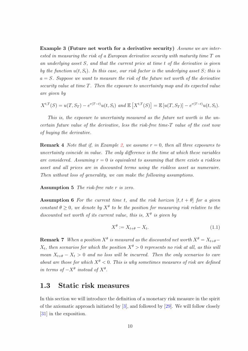
Example 3 (Future net worth for a derivative security) Assume we are inter-
ested in measuring the risk of a European derivative security with maturity time T on
an underlying asset S, and that the current price at time t of the derivative is given
by the function u(t, St). In this case, our risk factor is the underlying asset S; this is
a = S. Suppose we want to measure the risk of the future net worth of the derivative
security value at time T . Then the exposure to uncertainty map and its expected value
are given by
X t,T (S) = u(T, ST )− er(T−t)u(t, St) and E[X t,T (S)
]= E [u(T, ST )]− er(T−t)u(t, St).
This is, the exposure to uncertainty measured as the future net worth is the un-
certain future value of the derivative, less the risk-free time-T value of the cost now
of buying the derivative.
Remark 4 Note that if, in Example 2, we assume r = 0, then all three exposures to
uncertainty coincide in value. The only difference is the time at which these variables
are considered. Assuming r = 0 is equivalent to assuming that there exists a riskless
asset and all prices are in discounted terms using the riskless asset as numeraire.
Then without loss of generality, we can make the following assumptions.
Assumption 5 The risk-free rate r is zero.
Assumption 6 For the current time t, and the risk horizon [t, t + θ] for a given
constant θ ≥ 0, we denote by Xθ to be the position for measuring risk relative to the
discounted net worth of its current value, this is, Xθ is given by
Xθ := Xt+θ −Xt. (1.1)
Remark 7 When a position Xθ is measured as the discounted net worth Xθ = Xt+θ−Xt, then scenarios for which the position Xθ > 0 represents no risk at all, as this will
mean Xt+θ − Xt > 0 and no loss will be incurred. Then the only scenarios to care
about are those for which Xθ < 0. This is why sometimes measures of risk are defined
in terms of −Xθ instead of Xθ.
1.3 Static risk measures
In this section we will introduce the definition of a monetary risk measure in the spirit
of the axiomatic approach initiated by [3], and followed by [29]. We will follow closely
[31] in the exposition.
10
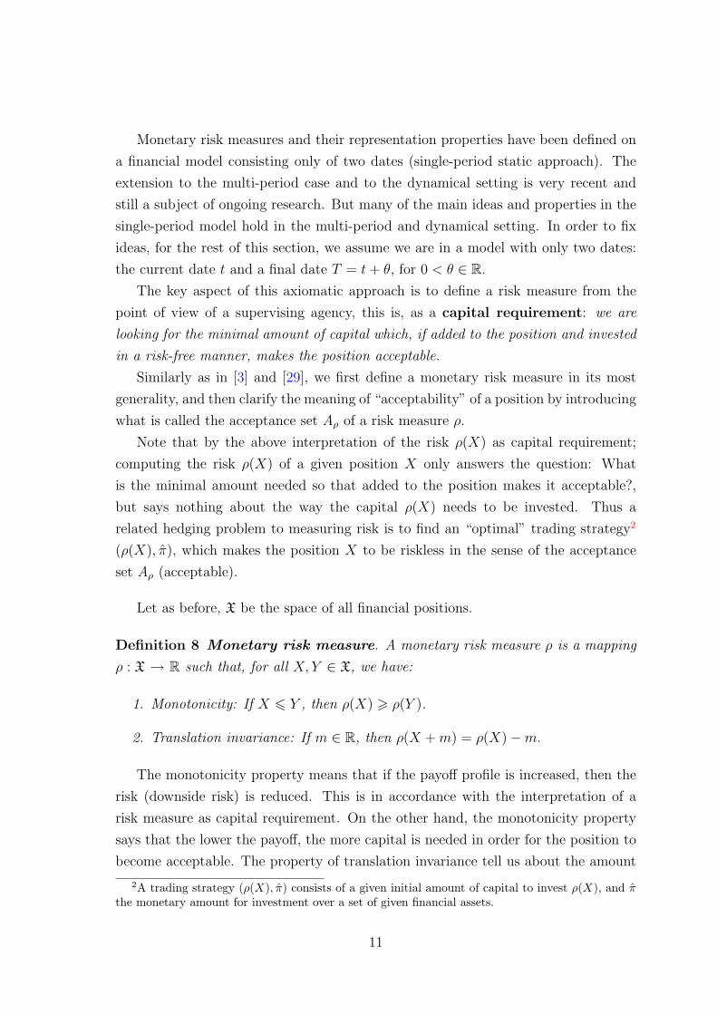
Monetary risk measures and their representation properties have been defined on
a financial model consisting only of two dates (single-period static approach). The
extension to the multi-period case and to the dynamical setting is very recent and
still a subject of ongoing research. But many of the main ideas and properties in the
single-period model hold in the multi-period and dynamical setting. In order to fix
ideas, for the rest of this section, we assume we are in a model with only two dates:
the current date t and a final date T = t+ θ, for 0 < θ ∈ R.
The key aspect of this axiomatic approach is to define a risk measure from the
point of view of a supervising agency, this is, as a capital requirement: we are
looking for the minimal amount of capital which, if added to the position and invested
in a risk-free manner, makes the position acceptable.
Similarly as in [3] and [29], we first define a monetary risk measure in its most
generality, and then clarify the meaning of “acceptability” of a position by introducing
what is called the acceptance set Aρ of a risk measure ρ.
Note that by the above interpretation of the risk ρ(X) as capital requirement;
computing the risk ρ(X) of a given position X only answers the question: What
is the minimal amount needed so that added to the position makes it acceptable?,
but says nothing about the way the capital ρ(X) needs to be invested. Thus a
related hedging problem to measuring risk is to find an “optimal” trading strategy2
(ρ(X), π), which makes the position X to be riskless in the sense of the acceptance
set Aρ (acceptable).
Let as before, X be the space of all financial positions.
Definition 8 Monetary risk measure. A monetary risk measure ρ is a mapping
ρ : X → R such that, for all X, Y ∈ X, we have:
1. Monotonicity: If X 6 Y , then ρ(X) > ρ(Y ).
2. Translation invariance: If m ∈ R, then ρ(X +m) = ρ(X)−m.
The monotonicity property means that if the payoff profile is increased, then the
risk (downside risk) is reduced. This is in accordance with the interpretation of a
risk measure as capital requirement. On the other hand, the monotonicity property
says that the lower the payoff, the more capital is needed in order for the position to
become acceptable. The property of translation invariance tell us about the amount
2A trading strategy (ρ(X), π) consists of a given initial amount of capital to invest ρ(X), and πthe monetary amount for investment over a set of given financial assets.
11
of money which should be added to the position in order to make it acceptable from
the point of view of a supervisory agency. Thus, if the amount m is added to the
position and invested in a risk-free manner, the capital requirement is reduced by the
same amount. Many authors define a risk measure only as the corresponding map ρ
without the monotonicity and translation invariance properties. But it turns out that
most of the risk measures in practise, particularly the ones analysed in this thesis,
satisfy these two properties, thus the equivalence in the definitions.
Remark 9 For a position Xθ := Xt+θ −Xt and a risk interval [t, t + θ], the second
term on the right-hand side of Xθ is a deterministic quantity. Then the randomness
of Xθ is only due to the term Xt+θ, and by the translation invariance property of the
risk measures, there is no difference in analysing Xθ or Xt+θ. Therefore, without loss
of generality, throughout this document we concentrate our analysis as if Xθ = Xt+θ,
unless otherwise made explicit. Also, whenever there is no room for confusion, we
will also omit the explicit dependence of X on θ, writing X when we mean Xθ.
Remark 10 The cash invariance property implies ρ(X + ρ(X)) = ρ(X)− ρ(X) = 0,
and ρ(m) = ρ(0)−m for all m ∈ R. This suggests assuming a normalisation whereby
ρ(0) = 0.
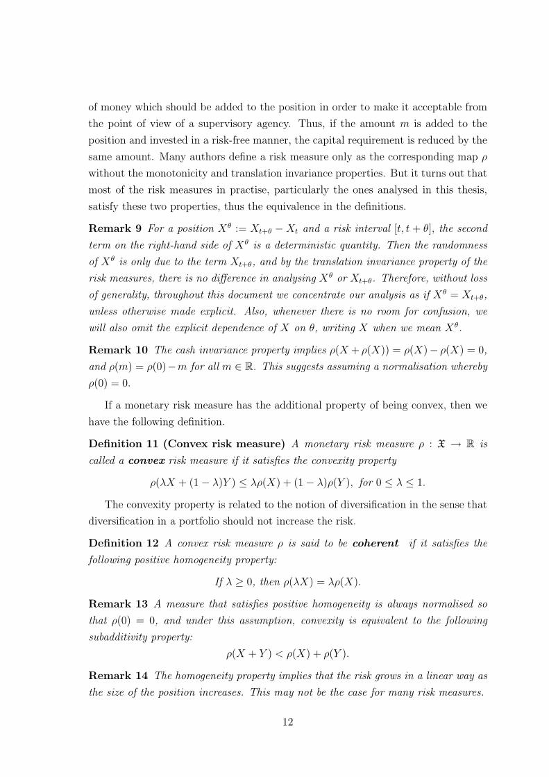
If a monetary risk measure has the additional property of being convex, then we
have the following definition.
Definition 11 (Convex risk measure) A monetary risk measure ρ : X → R is
called a convex risk measure if it satisfies the convexity property
ρ(λX + (1− λ)Y ) ≤ λρ(X) + (1− λ)ρ(Y ), for 0 ≤ λ ≤ 1.
The convexity property is related to the notion of diversification in the sense that
diversification in a portfolio should not increase the risk.
Definition 12 A convex risk measure ρ is said to be coherent if it satisfies the
following positive homogeneity property:
If λ ≥ 0, then ρ(λX) = λρ(X).
Remark 13 A measure that satisfies positive homogeneity is always normalised so
that ρ(0) = 0, and under this assumption, convexity is equivalent to the following
subadditivity property:
ρ(X + Y ) < ρ(X) + ρ(Y ).
Remark 14 The homogeneity property implies that the risk grows in a linear way as
the size of the position increases. This may not be the case for many risk measures.
12
1.3.1 Acceptance sets and risk measures
We now introduce the notion of acceptability of a position given by a risk measure.
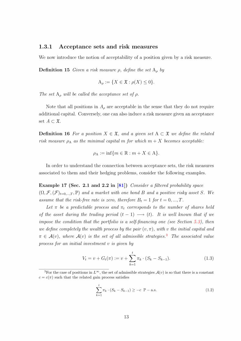
Definition 15 Given a risk measure ρ, define the set Aρ by
Aρ := X ∈ X : ρ(X) ≤ 0.
The set Aρ will be called the acceptance set of ρ.
Note that all positions in Aρ are acceptable in the sense that they do not require
additional capital. Conversely, one can also induce a risk measure given an acceptance
set A ⊂ X.
Definition 16 For a position X ∈ X, and a given set A ⊂ X we define the related
risk measure ρA as the minimal capital m for which m+X becomes acceptable:
ρA := infm ∈ R : m+X ∈ A.
In order to understand the connection between acceptance sets, the risk measures
associated to them and their hedging problems, consider the following examples.
Example 17 (Sec. 2.1 and 2.2 in [81]) Consider a filtered probability space
(Ω,F , (F)t=0,...,T ,P) and a market with one bond B and a positive risky asset S. We
assume that the risk-free rate is zero, therefore Bt = 1 for t = 0, ..., T .
Let π be a predictable process and πt corresponds to the number of shares held
of the asset during the trading period (t − 1) −→ (t). It is well known that if we
impose the condition that the portfolio is a self-financing one (see Section 5.3), then
we define completely the wealth process by the pair (v, π), with v the initial capital and
π ∈ A(v), where A(v) is the set of all admissible strategies.3 The associated value
process for an initial investment v is given by
Vt = v +Gt(π) := v +t∑
k=1
πk · (Sk − Sk−1). (1.3)
3For the case of positions in L∞, the set of admissible strategies A(v) is so that there is a constantc = c(π) such that the related gain process satisfies
t∑k=1
πk · (Sk − Sk−1) ≥ −c P− a.s. (1.2)
13
Assume we define a financial position X ∈ L∞ to be acceptable if satisfies X ≥ 0
P-a.s. (if the risky part of X can be hedge at no additional cost). This means, we can
find a suitable hedging portfolio π such that
X +GT (π) ≥ 0 P− a.s.
This acceptability condition defines the acceptance set
A0 := X ∈ L∞ : ∃ π with X +GT (π) ≥ 0 P-a.s.,
and the corresponding risk measure ρ0 defined as
ρ0(X) := ρA0(X) = infm ∈ R : m+X ∈ A0.
Furthermore, if we assume that the market model is arbitrage-free, given the condition
infm ∈ R : m ∈ A0 > −∞ (see [81, Theorem 2.1]), then ρ0 can be represented
in terms of the set Me(P) of equivalent martingale measures for the price process S,
this is,
ρ0(X) = supQ∈Me(P)
EQ[−X].
Assume our investor is short in H ≥ 0 at time T (she must deliver the amount H at
time T ). On one hand, if we define psup(H) as
psup(H) := ρ0(−H) = supQ∈Me(P)
EQ[H],
and provided the right-hand side is finite, then psup(H) is equal to the cost of super-
replicating H, i.e., there exists a trading strategy π such that
psup(H) +GT (π) ≥ H P− a.s. (1.4)
On the other hand, by (1.3) for a given initial capital v and a trading strategy π ∈ A(v)
V(v,π)T = v +GT (π). (1.5)
Using ρ0, the risk of the short position is ρ0(−H). And from the interpretation of a
risk measure as the minimum amount of capital, the updated position ρ0(−H) − H
belongs to A0, this means, there exists a hedging portfolio π ∈ A(ρ0(−H)) such that
ρ0(−H)−H +GT (π) = V(ρ0(−H),π)T −H ≥ 0 P− a.s., (1.6)
which is equivalent to the expression in (1.4).
14
Although by performing such a superhedging strategy, the investor eliminates com-
pletely the corresponding risk, the disadvantage is that the initial amount psup(H) is
most of the time too high from a practical point of view. There is a disadvantage even
in the case where the claim is attainable, as the elimination of the risk goes together
with the elimination of the possibility of making any profit.
Let us therefore suppose that the investor is unwilling to put up the capital ρ0(−H)
and is ready to accept some risk. For a fixed v ∈ (0, psup(H)), this imply that for any
π ∈ A(v) there would exist some ω ∈ Ω such that
V(v,π)T (ω)−H(ω) ≥ 0 (superreplication/replication) (1.7)
and that some ω ∈ Ω where
V(v,π)T (ω)−H(ω) < 0 (no-replication). (1.8)
Then any hedging strategy will be “partial” in the sense of replication/superreplication.
In order to make the most of the previous situation, we can formulate a sensible
“partial” hedging problem by noting that it is desirable to find a hedging portfolio π
which deals only with the problematic events -those in (1.8)- and such that V(v,π)T is
as closest as possible to H. This is achieved by using the shortfall function(H − V
(v,π)T
)+
as it assigns zero to the superreplication/replication events and a positive quantity to
the no- replication events. And as the goal is to make this shortfall small, the general
“partial” hedging problem to solve is:4
Find a hedging strategy π ∈ A(v) which attains the infimum in
infπ∈A(v)
(H − V
(v,π)T
)+
,
with v ≤ v.
The above provided we give sufficient conditions so the random variable H −V
(v,π)T <∞; for example, guaranteeing that H − V
(v,π)T ∈ L0.
4The problem can also be generalised as in [81, Sec. 2.2] considering another suitable risk measureρ. Find a hedging strategy π ∈ A(v) which attains the infimum in
infπ∈A(v)
ρ
(−(H − V
(v,π)T
)+)
,
with v ≤ v.
15
Later in this chapter, we review briefly the hedging problems associated to the
risk measures Worst Conditional Scenario (WCS), Value-at-Risk (VaR) and Average
Value-at-Risk (AVaR), and in Chapter 5 we study in more detail the solution to the
hedging problem associated to the WCS risk measure.
1.3.2 Robust representation of convex risk measures
We recall now some important characterisations of coherent and convex risk measures
and their acceptance sets. For the case when X := L∞(Ω,F ,P), it has been proved in
[81] that any coherent risk measure measure can be interpreted as a sort of worst-case
scenario over a set of probability measures. This result is recalled in the following
proposition. For similar results in spaces other than L∞ or generalisations see for
example [3],[16], [15], [34], [35] [29] and [32].
Denote by Ma := Ma(P) := Ma(Ω,F ,P) the set of all probability measures Q on
(Ω,F) which are absolutely continuous with respect to P; and byMa,f := Ma,f (P) :=
Ma,f (Ω,F ,P) the set of all finitely additive set functions Q : F → [0, 1] which are
normalised to Q[Ω] = 1 and absolutely continuous with respect to P in the sense that
Q[A] = 0 if P[A] = 0.
Proposition 18 (Prop. 4.6 and 4.14 in [32] and Corollary 1.17 in [81]) The
following statements are equivalent.
1. A functional ρ : X = L∞(Ω,F ,P) → R is a coherent risk measure.
2. The acceptance set of ρ, A, is a cone.
3. ρ is a continuous from below: Xn X then ρ(Xn) ρ(X).
4. There exists a subset P ⊂Ma(P) representing ρ such that the supremum is
attained in
ρ(X) = supQ∈P
EQ [−X] , for all X ∈ L∞. (1.9)
The next proposition shows the analogous representation for convex risk measures.
Proposition 19 (Prop. 4.6 and Thm. 4.15 in [32] and Thm 1.10 in [81]) The
following statements are equivalent:
1. A functional ρ : X = L∞(Ω,F ,P) → R is a convex risk measure.
2. The acceptance set of ρ, A is convex.
16
3. ρ can be represented as
ρ(X) = supQ∈Ma,f (P)
EQ [−X]− αmin(Q) , X ∈ L∞, (1.10)
where the penalty function αmin is given by
αmin(Q) := supX∈Aρ
EQ [−X] for Q ∈Ma,f (P).
Moreover, αmin is the minimal penalty function which represents ρ, i.e., any
penalty function α for which (1.10) holds satisfies α(Q) ≥ αmin(Q) for all
Q ∈Ma,f (P).
The difference between the representation of a coherent and a convex risk measure
is that in the latter, the supremum is taken over a finer set of probability measures but
the effect that each measure Q has on the risk measure ρ is captured via the penalty
function α. For each measure Q, the penalty function α(Q) can be interpreted as the
worst value among all the acceptable positions computed under the measure Q.
We omit the proofs of the previous propositions as it is out of the scope of this
chapter, but we refer to [3],[16], [15], [34], [35] [29] and [32]. See also [31] for a general
account on monetary risk measures, their robust representation and properties.
1.4 Dynamic risk measures
The definition of a monetary risk measure and the axiomatic approach in the pre-
vious section has been presented in a single-period model. A natural extension of
this framework to the multi-period setting, or more generally to the continuous-time
setting, is to replace the expectation operator by a conditional expectation operator.
Thus, for any t ≤ τ ≤ T , the dynamical version (in continuous-time) of a convex risk
measure ρτ on the risk horizon [t, T ] will have the following representation
ρτ (X) = ess.supQ∈Ma,f (P) EQ [−X|Fτ ]− αmin(Q) , X ∈ L∞,
where the penalty function αmin is given by
αmin(Q) := supX∈Aρ(τ)
EQ [−X|Fτ ] for Q ∈Ma,f (P).
In a continuous-time setting, the dynamical version of a risk measure suggests the
introduction of the following time-consistency property.
17
Definition 20 A dynamic risk measure is said to be time-consistent on the risk hori-
zon [t, T ], if for any t ≤ T1 ≤ T and any position X ∈ X we have
ρt(X) = ρt(−ρT1(X)). (1.11)
The time-consistency property in the multi-period setting can be analogously de-
fined.
From the interpretation of a risk measure as a minimal capital requirement, the
time-consistency property implies that if at time t a position X is accepted with
respect to the risk measure ρ on the horizon [t, T ], then the position must also be
accepted at any other intermediate time T1, t ≤ T1 ≤ T , but with the risk measured
on the time horizon [T1, T ]. The minus sign in (1.11) is required because at time t
we need to measure the risk of a short position of value ρT1(X). For more on risk
measures and their properties see [5] or [32].
Remark 21 Without the minus sign in front of ρT1(X), the property of time-consistency
in (1.11) corresponds to the Bellman principle in dynamic programming.
In the next section, we introduce the three dynamic risk measures which we are
interested in, namely: the Worst-Case-Scenario measure (WCS), Value-at-
Risk (VaR), and Conditional Value-at-Risk (CVaR), their acceptance sets,
some properties and the related hedging problems.
1.5 The risk measures: WCS, VaR and AVaR
1.5.1 Worst-Case-Scenario
Assume we have fixed a probability triple (Ω,F ,P), and denote by M1 := M1(P) :=
M1(Ω,F ,P) the set of all probability measures on (Ω,F).
Definition 22 Worst-case scenario. Let P be a subset of M1. The worst-case
scenario risk measure over P for a position X is defined as:
WCSP(X) = supQ∈P
EQ [−X] (1.12)
i.e., the supremum of expected losses over a set of probability measures.
18
Its acceptance is given by
AWCSP := X ∈ X : supQ∈P
EQ [−X] ≤ 0. (1.13)
It is direct to see that it is a coherent risk measure.
One interpretation of WCSP(X) is to measure risk on stress-test scenarios, this is,
imagine one needs to know the effect that a set of chosen scenarios (turmoil situations,
new model estimations, etc.) has on the position X. This is done by computing the
expected value on the worst possible situation among the chosen scenarios P . Another
interpretation of WCSP is that by assuming P ∈P, then we can interpret WCSP as
the risk measure that incorporates uncertainty in the model, this is, when there is no
full knowledge of the probability structure of the model, but instead an approximation
in terms of a set of probability measures (robust preferences). A particular case of
the previous situation is assuming a model which may not be fully specified (e.g. a
parameter may only be known to lie in a given range). Then in order to be on the
safe side, one defines the expected values in terms of the worst possible case among
the models in P .Note that the risk given by WCSP depends directly on the choice of the set P ⊂
M1. In order to distinguish some important cases, define as before Ma := Ma(P) :=
Ma(Ω,F ,P) and analogously Me := Me(P) := Me(Ω,F ,P) as the set of absolutely
continuous and equivalent measures to the reference measure P, respectively, this is,
Ma :=
Q ∈M1 : ∃ a Radon-Nikodym derivative
dQdP
,
and
Me :=
Q ∈M1 : ∃ a Radon-Nikodym derivative
dQdP
> 0 P-a.s.
.
Some special cases of interest are taking P equal to M1,Ma,Me, and Q for a
given Q ∈M1.
When P = M1, the corresponding risk measure is called worst-case risk measure
as shown in the next example.
Example 23 (P = M1) Define the risk measure ρmax called the worst-case risk mea-
sure by
ρmax(X) := − infω∈Ω
X(ω) = infm ∈ R : m+X ≥ 0.
This measure is coherent and can be represented as
ρmax(X) = supQ∈M1
EQ [−X] .
19
For a given position X, the worst-case risk measure, as its name suggests, give us
an upper bound of the risk of the position measures by any other risk measure. It
gives the largest value we can get.
We now give some remarks on the rest of the special cases.
Remark 24 1. When P = Me, the set Me is convex but not compact; then if for
the position X we have EQ [X] < ∞ for each Q ∈ Me, the measure where the
supremum is attained will belong to Ma.
2. In the case where the set consists of only one measure, this is, P = Q for
Q ∈M1, then the problem reduces to find the expected value of the position −Xunder the measure Q. A particular situation is when taking P = P. In this
case, the risk measure represents the expected value of the position −X under
the physical (real) probability measure.
In Chapter 3 we will be specially interested in computing WCSP when P ⊂Me
as it has the interpretation of model risk.
1.5.1.1 The hedging problem
Consider a single-period financial market model on the time-horizon [t, T ], which
consists of a risky asset S and a bond B. We assume the risk-free rate is zero,
therefore Bt = BT = 1. The current price of the asset S is denoted by St, and its
price at time T is modelled as a nonnegative random variable ST on a given complete
probability space (Ω,F ,P).
A trading strategy is a predictable random vector (πB, π), where π corresponds
to the number of assets S held during the trading period [t, T ], and πB is the number
of assets invested in the bond B. For an initial capital v ≥ 0 the value of the wealth
v at time t defined by the trading strategy (πB, π) is
v = πB + πSt.
As the quantities πB and π are held constant during the time-period [t, T ], by time
T , the value of the wealth has changed to
VT = πB + πST .
A portfolio is called self-financing if the only changes in the portfolio are due to
changes in the asset values. In terms of the wealth values we have VT−v = π(ST−St).
20
In order to define the gain process GT (π) as in Example 17, and to make explicitly
the dependence of VT on v and π, we write
V(v,π)T = v + π(ST − St) =: v +GT (π). (1.14)
As we want a market model free of arbitrage opportunities (see [51, Ch. 5.8]) we
assume the portfolio is such that
V(v,π)T ≥ 0. (1.15)
Denote by A(v) the set of predictable random variables π that define a wealth
as in (1.14) and satisfy (1.15) for an initial capital v ≥ 0. Thus, any self-financing
portfolio V can be fully described by a pair (v, π), π ∈ A(v).
Assume the investor needs to pay the random amount HT ≥ 0 at time T . The
risk, measured by WCSP , of the short position in HT is WCSP(−HT ). By the inter-
pretation of risk as capital requirement, WCSP(−HT ) is the minimal capital so that
the total position WCSP(−HT )−HT is acceptable, i.e.,
WCSP(−HT )−HT ∈ AWCSP .
We are particularly interested in linking hedging strategies with the measurement
of risk, then by our assumption of an arbitrage-free model (i.e., GT (π) ≥ 0 P-a.s.
implies GT (π) = 0 P-a.s.), we want to find hedging portfolios π ∈ A(WCSP(−HT ))
such that satisfy
WCSP(−HT )−HT +GT (π) ∈ AWCSP .
Using the equality in (1.14), the above expression can also be rewritten as
V(WCSP (−HT ),π)T −HT ∈ AWCSP ,
or by the characterisation of the acceptance set for WCSP in (1.13), this is similar to
find a hedging portfolios π ∈ A(WCSP(−HT )) that satisfy
supQ∈P
EQ
[−(V
(WCSP (−HT ),π)T −HT )
]= sup
Q∈PEQ
[HT − V
(WCSP (−HT ),π)T
]≤ 0
Assume for a moment that the investor is only willing to put up an initial capital
v less than WCSP(−HT ), then for any π ∈ A(v) the position V(v,π)T −HT /∈ AWCSP ,
or equivalently
supQ∈P
EQ
[HT − V
(v,π)T
]> 0.
21
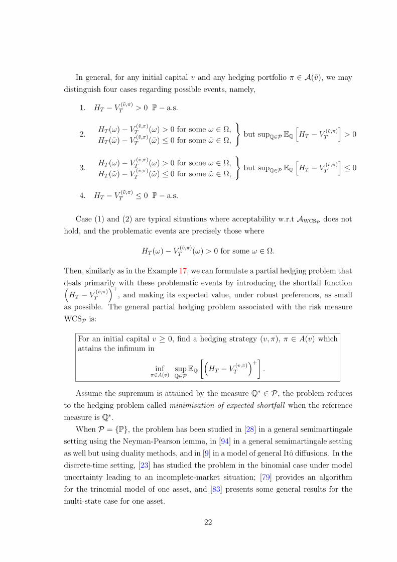
In general, for any initial capital v and any hedging portfolio π ∈ A(v), we may
distinguish four cases regarding possible events, namely,
1. HT − V(v,π)T > 0 P− a.s.
2.HT (ω)− V
(v,π)T (ω) > 0 for some ω ∈ Ω,
HT (ω)− V(v,π)T (ω) ≤ 0 for some ω ∈ Ω,
but supQ∈P EQ
[HT − V
(v,π)T
]> 0
3.HT (ω)− V
(v,π)T (ω) > 0 for some ω ∈ Ω,
HT (ω)− V(v,π)T (ω) ≤ 0 for some ω ∈ Ω,
but supQ∈P EQ
[HT − V
(v,π)T
]≤ 0
4. HT − V(v,π)T ≤ 0 P− a.s.
Case (1) and (2) are typical situations where acceptability w.r.t AWCSP does not
hold, and the problematic events are precisely those where
HT (ω)− V(v,π)T (ω) > 0 for some ω ∈ Ω.
Then, similarly as in the Example 17, we can formulate a partial hedging problem that
deals primarily with these problematic events by introducing the shortfall function(HT − V
(v,π)T
)+
, and making its expected value, under robust preferences, as small
as possible. The general partial hedging problem associated with the risk measure
WCSP is:
For an initial capital v ≥ 0, find a hedging strategy (v, π), π ∈ A(v) whichattains the infimum in
infπ∈A(v)
supQ∈P
EQ
[(HT − V
(v,π)T
)+].
Assume the supremum is attained by the measure Q∗ ∈ P , the problem reduces
to the hedging problem called minimisation of expected shortfall when the reference
measure is Q∗.
When P = P, the problem has been studied in [28] in a general semimartingale
setting using the Neyman-Pearson lemma, in [94] in a general semimartingale setting
as well but using duality methods, and in [9] in a model of general Ito diffusions. In the
discrete-time setting, [23] has studied the problem in the binomial case under model
uncertainty leading to an incomplete-market situation; [79] provides an algorithm
for the trinomial model of one asset, and [83] presents some general results for the
multi-state case for one asset.
22
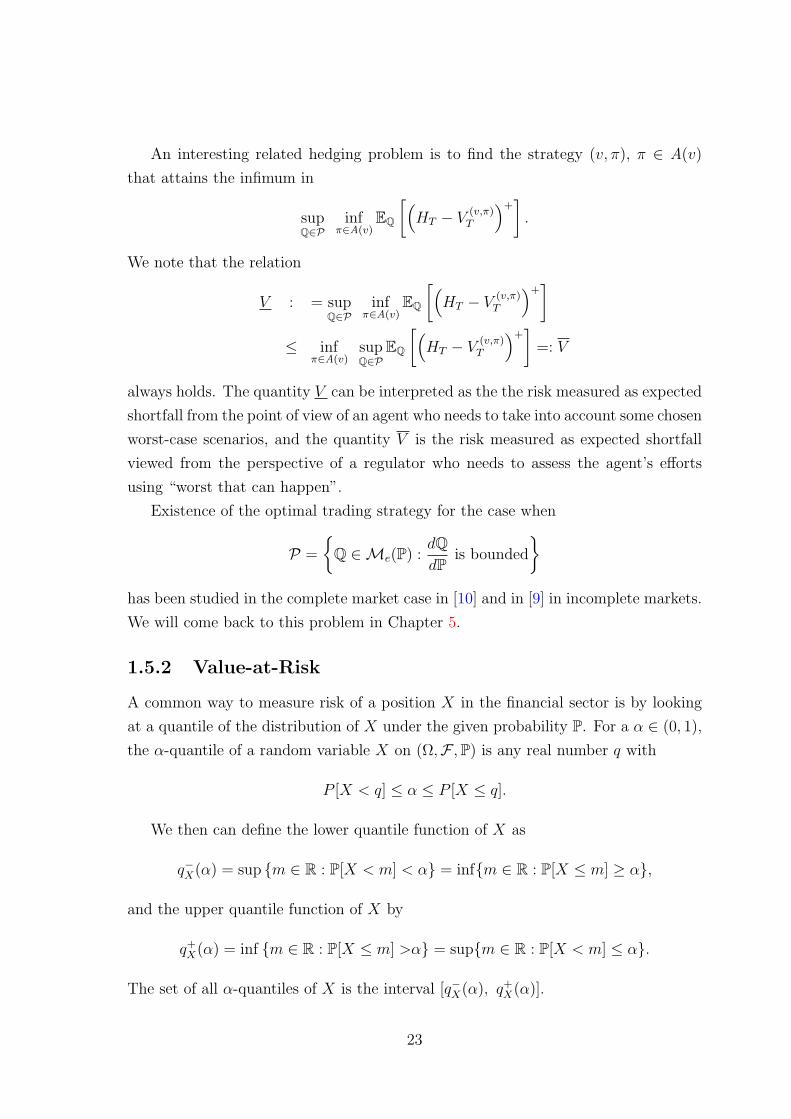
An interesting related hedging problem is to find the strategy (v, π), π ∈ A(v)
that attains the infimum in
supQ∈P
infπ∈A(v)
EQ
[(HT − V
(v,π)T
)+].
We note that the relation
V : = supQ∈P
infπ∈A(v)
EQ
[(HT − V
(v,π)T
)+]
≤ infπ∈A(v)
supQ∈P
EQ
[(HT − V
(v,π)T
)+]
=: V
always holds. The quantity V can be interpreted as the the risk measured as expected
shortfall from the point of view of an agent who needs to take into account some chosen
worst-case scenarios, and the quantity V is the risk measured as expected shortfall
viewed from the perspective of a regulator who needs to assess the agent’s efforts
using “worst that can happen”.
Existence of the optimal trading strategy for the case when
P =
Q ∈Me(P) :
dQdP
is bounded
has been studied in the complete market case in [10] and in [9] in incomplete markets.
We will come back to this problem in Chapter 5.
1.5.2 Value-at-Risk
A common way to measure risk of a position X in the financial sector is by looking
at a quantile of the distribution of X under the given probability P. For a α ∈ (0, 1),
the α-quantile of a random variable X on (Ω,F ,P) is any real number q with
P [X < q] ≤ α ≤ P [X ≤ q].
We then can define the lower quantile function of X as
q−X(α) = sup m ∈ R : P[X < m] < α = infm ∈ R : P[X ≤ m] ≥ α,
and the upper quantile function of X by
q+X(α) = inf m ∈ R : P[X ≤ m] >α = supm ∈ R : P[X < m] ≤ α.
The set of all α-quantiles of X is the interval [q−X(α), q+X(α)].
23
Definition 25 VaR. Given α ∈ (0, 1), the value at risk at a level α of a random
variable X on (Ω,F ,P) is given by
VaRα(X) = infm ∈ R : P[X +m < 0] ≤ α = −q+X(α) = q−−X(1− α).
VaRα can be interpreted as the “smallest” value such that the probability of the
absolute loss being at most this value is at least 1 − α. Then 95% and 99% VaR
corresponds to taking α = 0.05 and α = 0.01, respectively. Note that VaR is blind
toward risks that create large losses with a very small probability (below the critical
probability level α). For a good general account of VaR and its estimation methods
with discrete data see for example [19], for some properties and pitfalls of VaR see
[66], [74], [72], [93] [48], and [91].
In term of risk measures as capital requirement, VaRα can be also interpreted as
the minimal amount of capital that an investor needs to reserve in order to cover for
potential losses with a confidence given by α. In order to see more clearly how VaRα
works, assume the position X has zero risk measured as VaRα then we have P[XT <
Xt] ≤ α. It means that among the events of sure loss (those with XT − Xt < 0),
we only take as acceptable the events that have lower or equal probability than the
chosen level α.
One can show that VaRα satisfies the property of translation invariance, it is posi-
tive homogeneous, monotone decreasing but not a convex risk measure (for examples
showing that VaR is not convex see [3], [15], [16] or [31]). The fact that VaRα is not
convex means that VaRα penalise diversification instead of encouraging it in some
models.
We have defined VaRα only for positions, but as we will extensively be using the
notation Xθ := Xt+θ −Xt to represent a position for measuring risk on the interval
[t, t + θ], and as the only random component on Xθ comes from Xt+θ; it is useful to
relate VaRα(Xθ) with the value of the upper α-quantile of Xt+θ (i.e., q+Xt+θ
(α) ). See
also Figure 1.1
Proposition 26 Given α ∈ (0, 1) fixed, the VaRα of the position Xθ can be related
with q+Xt+θ
(α) as follows:
VaRα(Xθ) = Xt − q+Xt+θ
(α).
Proof. It follows from the definition.
The acceptance set for VaRα is
AVaRα :=X ∈ L0 : VaRα(X) ≤ 0
=X ∈ L0 : q+
X(α) ≥ 0. (1.16)
24
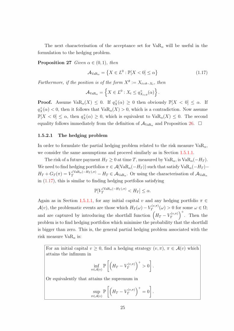
The next characterisation of the acceptance set for VaRα will be useful in the
formulation to the hedging problem.
Proposition 27 Given α ∈ (0, 1), then
AVaRα =X ∈ L0 : P[X < 0] ≤ α
(1.17)
Furthermore, if the position is of the form Xθ := Xt+θ−Xt, then
AVaRα =X ∈ L0 : Xt ≤ q+
Xt+θ(α).
Proof. Assume VaRα(X) ≤ 0. If q+X(α) ≥ 0 then obviously P[X < 0] ≤ α. If
q+X(α) < 0, then it follows that VaRα(X) > 0, which is a contradiction. Now assume
P[X < 0] ≤ α, then q+X(α) ≥ 0, which is equivalent to VaRα(X) ≤ 0. The second
equality follows immediately from the definition of AVaRα and Proposition 26.
1.5.2.1 The hedging problem
In order to formulate the partial hedging problem related to the risk measure VaRα,
we consider the same assumptions and proceed similarly as in Section 1.5.1.1.
The risk of a future paymentHT ≥ 0 at time T , measured by VaRα, is VaRα(−HT ).
We need to find hedging portfolios π ∈ A(VaRα(−HT )) such that satisfy VaRα(−HT )−HT +GT (π) = V
(VaRα(−HT ),π)T −HT ∈ AVaRα . Or using the characterisation of AVaRα
in (1.17), this is similar to finding hedging portfolios satisfying
P[V(VaRα(−HT ),π)T < HT ] ≤ α.
Again as in Section 1.5.1.1, for any initial capital v and any hedging portfolio π ∈A(v), the problematic events are those which HT (ω)−V (v,π)
T (ω) > 0 for some ω ∈ Ω;
and are captured by introducing the shortfall function(HT − V
(v,π)T
)+
. Then the
problem is to find hedging portfolios which minimise the probability that the shortfall
is bigger than zero. This is, the general partial hedging problem associated with the
risk measure VaRα is:
For an initial capital v ≥ 0, find a hedging strategy (v, π), π ∈ A(v) whichattains the infimum in
infπ∈A(v)
P[(HT − V
(v,π)T
)+
> 0
].
Or equivalently that attains the supremum in
supπ∈A(v)
P[(HT − V
(v,π)T
)+
= 0
].
25
Note that we could also have formulated the following less restrictive partial hedg-
ing problem
For an initial capital v ≥ 0, find a hedging strategy (v, π), π ∈ A(v) whichattains the infimum in
infπ∈A(v)
P[V
(v,π)T < HT
].
Or equivalently that attains the supremum in
supπ∈A(v)
P[V
(v,π)T ≥ HT
].
This hedging criteria are useful when the investor is interested in finding a hedging
strategy that overcomes a future value liability but on the most possible scenarios.
This fact is captured when maximising the probability that the final value of the
wealth process is larger than the liability value.
The latter hedging problem is known in the literature as maximising the probability
of success. It has been studied in [27] in a general semimartingale setting using the
Neyman-Pearson lemma, in [85] in a model of general Ito diffusions, and in [44] in an
incomplete market with two correlated assets given by geometric Brownian motions.
Another related hedging problem of interest is the so called minimising the cost
for a given probability of success:
Find the minimal initial capital v such that
P[V
(v,π)T ≥ HT
]≥ 1− α
holds.
1.5.3 Average Value-at-Risk
Given α ∈ (0, 1), one of the mayor drawbacks of VaRα is that it does not put any
attention to the losses that occur with probability smaller than the critical level α.
A natural alternative to overcome this problem is to define a risk measure by taking
the average of losses with probability levels less or equal to the critical level α. The
resulting measure is sometimes called Expected Shortfall, Conditional Value-at-Risk,
or Average Value-at-Risk. We adopt the latter name.
It has been shown, see for example [74], [72], [93], [89], and [2], that AVaR is a
risk measure that possesses better qualities than VaR. It is defined as follows.
26
Definition 28 The Average Value-at-Risk at a level α ∈ (0, 1] of a position X
is given by
AVaRα(X) :=1
α
α∫0
VaRγ(X)dγ.
Similarly, for a r.v. Xt+θ that comes from a position with representation Xθ :=
Xt+θ −Xt, we define the average upper α-quantile q+Xt+θ
(α) by
q+Xt+θ
(α) :=1
α
α∫0
q+Xt+θ
(γ)dγ.
In terms of capital requirement, AVaRα can be interpreted as the amount of capital
that needs to be reserved in order to cover in average the potential losses that have
a probability of occurrence of α or below.
The integral appearing in the definition of AVaRα is very inconvenient for com-
putation purposes, therefore we need to recall some other characterisations that are
easier to handle.
Let [x]+ represent the positive part of x, and [x]− its negative part.
Proposition 29 (Lemma 1.31 in [81]) Characterisation for AVaRα. Given
α ∈ (0, 1) fixed, and q an α-quantile of X, we have the following characterisations
for AVaRα:
AVaRα(X) =1
αE[(q −X)+
]− q
=1
αE[(−VaRα(X)−X)+
]+ VaRα(X).
Furthermore, if the position is of the form Xθ := Xt+θ −Xt, then
AVaRα(X) = Xt − q+Xt+θ
(α).
Proof. Take q = q+X(α), we have
1
αE[(q −X)+
]− q =
1
α
∫ 1
0
(q+X(α)− q+
X(t))+
dt− q+X(α)
=1
α
∫ α
0
max(−q+X(α),−q+
X(t))dt +1
α
∫ 1
α
max(q+X(α)− q+
X(t), 0)dt
=1
α
∫ α
0
−min(q+X(α), q+
X(t))dt +
1
α
∫ 1
α
max(q+X(α)− q+
X(t), 0)dt
=1
α
∫ α
0
−q+X(t)dt
= AVaRα(X).
27
The rest of the equalities follow directly from the definition of q+Xt+θ
(α), Xθ and the
fact that 1αE[(q+Xt+θ
(α)−Xt+θ
)+]− q+
Xt+θ(α) = −q+
Xt+θ(α).
For more details on different characterisations for AVaRα see [74], [93], [89], [2]
and [29].
Note that the original definition of AVaRα is to take an average of the Value-at-
Risk of the position X, over all the critical levels λ > 0 up to α. The characterisation
in the previous proposition exploits the fact that in AVaRα the only scenarios that
matter are those where X falls below VaRα(X) in average, but this is exactly the
same as taking the expectation of the random variable (X − VaRα(X))−.
It turns out that AVaRα is a coherent risk measure as shown in the next proposition
(see [32, Theo. 4.47 and Rmk. 4.84] and [81, Theo. 1.32 and Rmk. 1.34]).
Proposition 30 For α ∈ (0, 1), AVaRα is a coherent risk measure which is continu-
ous from below. It has the representation
AVaRα(X) = maxQ∈Pα
EQ[−X], X ∈ L1, (1.18)
where Pα is the set of all probability measures Q ∈ Ma whose density dQdP is P-
a.s. bounded by 1α. Furthermore, the maximum in (1.18) is attained by a measure
QAVaRα ∈Ma, whose density is given by
dQAVaRα
dP=
1
α
(1X <q + k1X =q
), (1.19)
where q is a α-quantile of X, and where k is defined as
k :=
0 if P[X = q] =0
α−P[X<q]P[X=q]
otherwise.(1.20)
Corollary 31 (Cor. 4.49 in [32] and Cor. 1.35 in [81]) For all X ∈ L∞,
AVaRα(X) ≥ E[−X : −X ≥ VaRα(X)]
≥ sup E[−X : A] : P[A] > α
≥ VaRα(X).
The first two inequalities are identities if P[X ≤ q+
X(α)]
= α.
Remark 32 The measure AVaRα is just a particular case of the WCSP(X) risk
measure by taking P = Pα.
28
The acceptance set corresponding to AVaRα is
AAVaRα :=X ∈ L1 : AVaRα(X) ≤ 0
=
X ∈ L1 :
1
αE[(−X − VaRα(X))+
]+ VaRα(X) ≤ 0
=
X ∈ L1 : max
Q∈Pα
EQ[X] ≥ 0
=
X ∈ L1 : EQAVaRα
[X] ≥ 0
=
X ∈ L1 : E
[X
α
(1X <q + k1X =q
)]≥ 0
,
for q an α-quantile of X and k defined in (1.20).
1.5.3.1 The hedging problem
Assume an investor needs to pay the random amount HT ≥ 0 at time T , and the
same assumptions in the Section 1.5.1.1 hold. As in the case for WCS, we can deduce
similarly that the associated hedging problem for AVaRα is the hedging problem of
minimisation of expected shortfall under robust preferences when the set of measures
is Pα. This is, the related partial hedging problem can be formulated as follows:
For an initial capital v ≥ 0, find a hedging strategy (v, π), π ∈ A(v) whichattains the infimum in
infπ∈A(v)
supQ∈Pα
EQ
[(HT − V
(v,π)T
)+].
1.6 Superreplication and partial hedging
In the previous section we have formulated the hedging problems associated with the
three risk measures WCS, VaR and AVaR without assuming anything on the financial
market (complete or incomplete market model, etc.). Assume we work on a time
horizon [t, T ] and under a complete and filtered probability space (Ω,F , (F)t≤τ≤T , P).
If the market is complete and free of arbitrage opportunities, any contingent claim HT
with fixed payoff at time T can be replicated or hedged by a trading strategy (v, π)
consisting of an initial capital v ≥ 0 and a dynamical portfolio process π ∈ A(v).
When the market is not complete, for example, when insufficient number of assets
are available for investment, then the existence of a replicating process (v, π) cannot
29
always be guaranteed, unless the investor is prepared to hold an initial capital equal
to the super-replicating price
supQ∈Me
EQ [HT ] ,
where Me denotes the set of all equivalent martingale measures with respect to the
probability P.
In this case, the risk involved in the investment HT can be completely eliminated
because a super-hedging strategy can be performed. On the other hand, when the
investor is only willing to put up a smaller amount of the initial capital
v ∈(
0, supQ∈Me
EQ [HT ]
),
then a non-hedgeable risk will be involved and any hedging strategy (v, π) will be
“partial” in the sense that its shortfall
(HT − VT )+
may be non zero with positive probability.
In the more general setting one can formulate the partial hedging problem not
only by looking at the shortfall S := (HT − VT )+, but any other similar criterion.
Popular choices of criterion for hedging in incomplete markets are: maximise the
expected utility U of the difference −D := VT − HT , minimise the risk of D or of
the shortfall S by a convex risk functional, this is l(D) or l(S), respectively (for some
examples of risk measures in terms of the expected shortfall see Appendix A.2).
In relation to the hedging problems associated with WCS, VaR and AVaR the
chosen criterion is S := (HT − VT )+, and in order to specify a pure partial hedging
situation one need to incorporate the initial capital constraints.
The partial hedging problem for WCS need to be rewritten as follows:
For a fixed amount v,
v ∈(
0, supQ∈M
EQ [HT ]
),
and an initial capital v ≥ v ≥ 0, find a hedging strategy (v, π), π ∈ A(v)which attains the infimum in
infπ∈A(v)
supQ∈P
EQ
[(HT − V
(v,π)T
)+].
30
For the risk measure VaR, we have
For a fixed amount v,
v ∈(
0, supQ∈M
EQ [HT ]
),
and an initial capital v ≥ v ≥ 0, find a hedging strategy (v, π), π ∈ A(v)which attains the infimum in
infπ∈A(v)
P[(HT − V
(v,π)T
)+
> 0
].
Or equivalently that attains the supremum in
supπ∈A(v)
P[(HT − V
(v,π)T
)+
= 0
].
Or alternatively,
For a fixed amount v,
v ∈(
0, supQ∈M
EQ [HT ]
),
and an initial capital v ≥ v ≥ 0, find a hedging strategy (v, π), π ∈ A(v)which attains the infimum in
infπ∈A(v)
P[V
(v,π)T < HT
].
Or equivalently that attains the supremum in
supπ∈A(v)
P[V
(v,π)T ≥ HT
].
The AVaR partial hedging problem becomes
For a fixed amount v,
v ∈(
0, supQ∈M
EQ [HT ]
),
and an initial capital v ≥ v ≥ 0, find a hedging strategy (v, π), π ∈ A(v)which attains the infimum in
infπ∈A(v)
supQ∈Pα
EQ
[(HT − V
(v,π)T
)+].
31
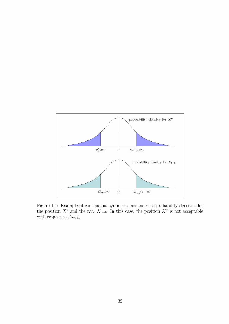
Figure 1.1: Example of continuous, symmetric around zero probability densities forthe position Xθ and the r.v. Xt+θ. In this case, the position Xθ is not acceptablewith respect to AVaRα .
32
Part I
Risk and Hedging in Discrete-time:A Two-factor Binomial Model
33
Chapter 2
Minimisation of Expected Shortfall
2.1 Introduction
Assume we work on the time horizon [0, T ] in a complete and filtered probability
space (Ω,F , (F)0≤t≤T , P), and that an investor faces a random liability H ≥ 0 at
time T . In this chapter, we are interested in the following partial hedging problem:
For a fixed initial capital v ∈(
0, supQ∈Me
EQ [HT ]
), the problem is to find a trading
strategy (v, π), with v ≤ v and π ∈ A(v) such that the expected shortfall
EP[(HT − VT )+
](2.1)
is minimal under the physical probability measure P.
This problem has been studied in the context of semimartingale processes and
general Ito diffusions (see [9], [28] and [31, p. 341]) in the sense that the authors have
shown existence and general characterisation of the solution (the trading strategy
and the minimal expected shortfall). It turns out that the solution to the minimal
expected shortfall problem can be divided into two parts: the solution to a “static-
hedging” problem of minimising
EP[(HT − Y )+
]among all FT -measurable random variables Y ≥ 0 which satisfy the constraint
supQ∈M
EQ [Y ] ≤ v.
If Y ∗ denotes the solution in the first part, then the second part consists in fitting the
terminal value VT of an admissible strategy to the optimal solution Y ∗ . This will be
recalled in more detail in Section 2.2.
34
This two-steps solutions is intuitively clear as the optimisation criterion involves
only values at time T , therefore, minimising only over FT -measurable random vari-
ables is equivalent, with the condition supQ∈M
EQ [Y ] ≤ v needed to guarantee that we
could match the value of the minimiser Y ∗ to a dynamical hedging strategy with
initial value less than the constraint threshold v.
Although it has been shown that the solution exists and is characterised via the
above two-step procedure, few explicit solutions or approximating algorithms have
been studied in the literature. They will rely of course on the particular model
assumed. In the discrete-time setting, [23] has studied the problem in the binomial
case under model uncertainty leading to an incomplete-market situation; [79] provides
an algorithm for the trinomial model of one asset, and [83] presents some general
results for the multi-state case for one asset.
Because our interest is in real options (when there are non-traded assets in the
market), in this chapter we analyse the problem in the basic setting of two correlated
assets (one traded and one non-traded). Also, with the goal of understanding the
nature of the solution and the optimal strategies, and in order to be able to compute
explicitly the strategies and the expected shortfall, we will assume a discrete-time
model of two correlated N -period binomial trees. We show how even in this the
simplest discrete-time approximation of a continuous time-model it is difficult to find
in general an explicit solution to the problem, as the key issue in the solution is that
the value function preserves the same form at each time step.
2.2 The two-step procedure in the minimisation of
expected shortfall
The core of the problem of minimising the expected shortfall in (2.1) is to find a
dynamic self-financing trading strategy which solves a static optimisation problem
(of a terminal value). This feature of dynamically-hedging a static position is also
reflected in the shape of the solution to the problem in (2.1) (see [9], [28]). It suggests
decomposing the problem into two parts:
1. The static optimisation problem: replace the terminal value of the (dynamic)
trading strategy by an appropriate (static) random variable, and
2. The dynamic-hedging strategy: perform a dynamic replicating trading strategy
on the modified claim.
35
In order to formulate the problem as a two-step procedure, we need some defini-
tions beforehand.
Definition 33 (Def 1 in [83]) Let
V∞ := V : V ≤ HT and EQ [V ] ≤ v for all Q ∈M
denote the set of all modified contingent claims for which the price of their super-
replicating strategy is less than or equal to the initial capital.
Definition 34 (Def 1 in [83]) Let
Vb := V : HT − b ≤ V ≤ HT and EQ [V ] ≤ v for all Q ∈M
for all b ∈ R+, the set of all modified contingent claims for which b is an upper bound
for the shortfall (HT − V v,π)+ when π is the super-hedging strategy of V .
The problem of minimising expected shortfall can be written as
Proposition 35 (Prop 2 in [83]) Let V ∈ Vb for b ≥ supQ∈M
EQ [HT ] − v denote a
modified contingent claim which is optimal in the sense that
V = arg minV ∈Vb
E [HT − VT ] .
Then the optimal expected shortfall strategy π of the problem in (2.1) is the super-
replicating strategy for the claim V :
E[HT − V v,π
T
]= min
A(v)E[(HT − V v,π)+] = E
[HT − V
].
Proof. See [28] for the proof in continuous-time general semimartingale setting, [67]
in a discrete-time setting, and [83] in the context of discrete time single asset.
The above proposition justifies the following two-step procedure proposed in [83].
STEP 1 (static optimisation problem) Find an optimal modified contingent claim
V ∈ Vb with V = arg minV ∈VbE [HT − V ].
STEP 2 (Representation problem) Determine the super-replicating strategy of
V .
Equivalently, STEP 1 above can be characterised as
36
Proposition 36 The static optimisation problem in STEP 1 is equivalent to solving
max E [V ]
under the constraints
HT − b ≤ V ≤ HT and supQ∈M
EQ [V ] ≤ v.
Remark 37 The formulation of the problem of minimising expected shortfall in Propo-
sition 36 highlights the strong relation with the problem of maximising the probability
of a perfect hedge. This can be seen as follows. By the constraint HT − b ≤ V ≤ HT ,
the maximisation of E [V ] will give an value V ∗ close to HT in their expected values,
but this is equivalent to maximising the probability that V is bigger than the payoff
HT , therefore establishing the relation between the two problems.
In the rest of the section, we will analyse the problem in the basic setting of two
correlated assets (one traded and one non-traded). Also, with the goal of under-
standing the nature of the solution and the optimal strategies, and in order to be
able to compute explicitly the strategies and the expected shortfall, we will assume a
discrete-time model of two correlated N -period binomial trees.
2.3 The two-factors N-period binomial model for
the expected shortfall
Consider a N -period model on the horizon [0, N ] consisting of one riskless and two
risky assets. Only one of the risky assets is considered to be traded in the market.
Let us denote by S0 and Y0 the values of the traded (stock) and non traded asset
at time zero, respectively. At the end of each period [n, n + 1], n = 0, ..., N − 1,
the traded asset can only take two values Sn+1 = Snξn+1, where ξn+1n=0,...,N−1 is a
sequence of i.i.d. random variables taking values in the set u, d with 0 < d < 1 < u
for n = 0, ..., N − 1. In a similar manner, the value of the non-traded asset satisfies
Yn+1 = Ynηn+1, where as before, ηn+1n=0,...,N−1 is a sequence of i.i.d. random
variables with values in the set h, l, with l < h for n = 0, ..., N − 1.
We are interested in the two-dimensional stochastic process (Sn, Yn)0≤n≤N defined
on a probability space (Ω, (Fn)0≤n≤N ,P), where the filtration Fn is generated by the
random variables Sn+1, Yn+1, n = 0, ..., N−1, or equivalently by the random variables
37
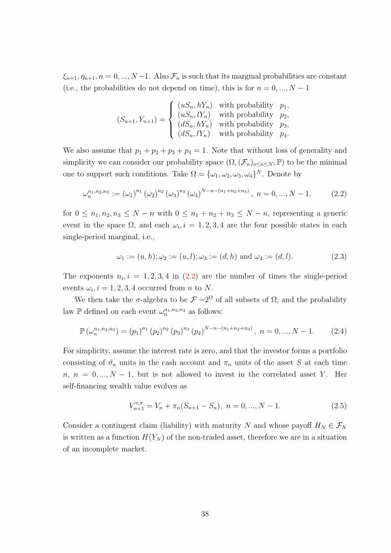
ξn+1, ηn+1, n = 0, ..., N−1. Also Fn is such that its marginal probabilities are constant
(i.e., the probabilities do not depend on time), this is for n = 0, ..., N − 1
(Sn+1, Yn+1) =
(uSn, hYn) with probability p1,(uSn, lYn) with probability p2,(dSn, hYn) with probability p3,(dSn, lYn) with probability p4.
We also assume that p1 + p2 + p3 + p4 = 1. Note that without loss of generality and
simplicity we can consider our probability space (Ω, (Fn)o≤n≤N ,P) to be the minimal
one to support such conditions. Take Ω = ω1, ω2, ω3, ω4N . Denote by
ωn1,n2,n3n := (ω1)
n1 (ω2)n2 (ω3)
n3 (ω4)N−n−(n1+n2+n3) , n = 0, ..., N − 1, (2.2)
for 0 ≤ n1, n2, n3 ≤ N − n with 0 ≤ n1 + n2 + n3 ≤ N − n, representing a generic
event in the space Ω, and each ωi, i = 1, 2, 3, 4 are the four possible states in each
single-period marginal, i.e.,
ω1 := (u, h);ω2 := (u, l);ω3 := (d, h) and ω4 := (d, l). (2.3)
The exponents ni, i = 1, 2, 3, 4 in (2.2) are the number of times the single-period
events ωi, i = 1, 2, 3, 4 occurred from n to N .
We then take the σ-algebra to be F =2Ω of all subsets of Ω, and the probability
law P defined on each event ωn1,n2,n3n as follows:
P (ωn1,n2,n3n ) = (p1)
n1 (p2)n2 (p3)
n3 (p4)N−n−(n1+n2+n3) , n = 0, ..., N − 1. (2.4)
For simplicity, assume the interest rate is zero, and that the investor forms a portfolio
consisting of ϑn units in the cash account and πn units of the asset S at each time
n, n = 0, ..., N − 1, but is not allowed to invest in the correlated asset Y . Her
self-financing wealth value evolves as
V v,πn+1 = Vn + πn(Sn+1 − Sn), n = 0, ..., N − 1. (2.5)
Consider a contingent claim (liability) with maturity N and whose payoff HN ∈ FN
is written as a function H(YN) of the non-traded asset, therefore we are in a situation
of an incomplete market.
38
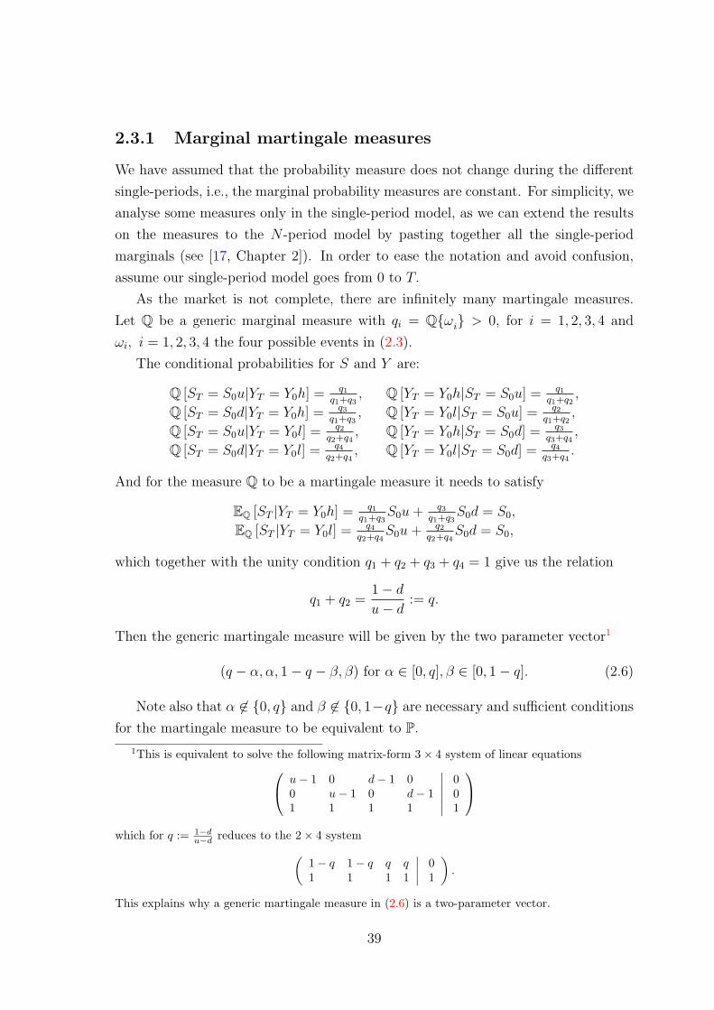
2.3.1 Marginal martingale measures
We have assumed that the probability measure does not change during the different
single-periods, i.e., the marginal probability measures are constant. For simplicity, we
analyse some measures only in the single-period model, as we can extend the results
on the measures to the N -period model by pasting together all the single-period
marginals (see [17, Chapter 2]). In order to ease the notation and avoid confusion,
assume our single-period model goes from 0 to T.
As the market is not complete, there are infinitely many martingale measures.
Let Q be a generic marginal measure with qi = Qωi > 0, for i = 1, 2, 3, 4 and
ωi, i = 1, 2, 3, 4 the four possible events in (2.3).
The conditional probabilities for S and Y are:
Q [ST = S0u|YT = Y0h] = q1
q1+q3, Q [YT = Y0h|ST = S0u] = q1
q1+q2,
Q [ST = S0d|YT = Y0h] = q3
q1+q3, Q [YT = Y0l|ST = S0u] = q2
q1+q2,
Q [ST = S0u|YT = Y0l] = q2
q2+q4, Q [YT = Y0h|ST = S0d] = q3
q3+q4,
Q [ST = S0d|YT = Y0l] = q4
q2+q4, Q [YT = Y0l|ST = S0d] = q4
q3+q4.
And for the measure Q to be a martingale measure it needs to satisfy
EQ [ST |YT = Y0h] = q1
q1+q3S0u+ q3
q1+q3S0d = S0,
EQ [ST |YT = Y0l] = q4
q2+q4S0u+ q2
q2+q4S0d = S0,
which together with the unity condition q1 + q2 + q3 + q4 = 1 give us the relation
q1 + q2 =1− d
u− d:= q.
Then the generic martingale measure will be given by the two parameter vector1
(q − α, α, 1− q − β, β) for α ∈ [0, q], β ∈ [0, 1− q]. (2.6)
Note also that α 6∈ 0, q and β 6∈ 0, 1−q are necessary and sufficient conditions
for the martingale measure to be equivalent to P.
1This is equivalent to solve the following matrix-form 3× 4 system of linear equations u− 1 0 d− 1 00 u− 1 0 d− 11 1 1 1
∣∣∣∣∣∣001
which for q := 1−d
u−d reduces to the 2× 4 system(1− q 1− q q q1 1 1 1
∣∣∣∣ 01
).
This explains why a generic martingale measure in (2.6) is a two-parameter vector.
39
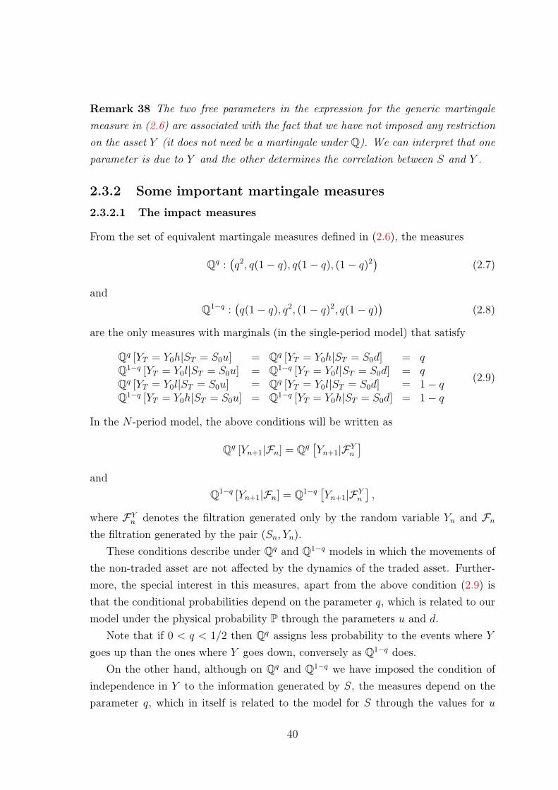
Remark 38 The two free parameters in the expression for the generic martingale
measure in (2.6) are associated with the fact that we have not imposed any restriction
on the asset Y (it does not need be a martingale under Q). We can interpret that one
parameter is due to Y and the other determines the correlation between S and Y .
2.3.2 Some important martingale measures
2.3.2.1 The impact measures
From the set of equivalent martingale measures defined in (2.6), the measures
Qq :(q2, q(1− q), q(1− q), (1− q)2
)(2.7)
and
Q1−q :(q(1− q), q2, (1− q)2, q(1− q)
)(2.8)
are the only measures with marginals (in the single-period model) that satisfy
Qq [YT = Y0h|ST = S0u] = Qq [YT = Y0h|ST = S0d] = qQ1−q [YT = Y0l|ST = S0u] = Q1−q [YT = Y0l|ST = S0d] = qQq [YT = Y0l|ST = S0u] = Qq [YT = Y0l|ST = S0d] = 1− qQ1−q [YT = Y0h|ST = S0u] = Q1−q [YT = Y0h|ST = S0d] = 1− q
(2.9)
In the N -period model, the above conditions will be written as
Qq [Yn+1|Fn] = Qq[Yn+1|FY
n
]and
Q1−q [Yn+1|Fn] = Q1−q[Yn+1|FY
n
],
where FYn denotes the filtration generated only by the random variable Yn and Fn
the filtration generated by the pair (Sn, Yn).
These conditions describe under Qq and Q1−q models in which the movements of
the non-traded asset are not affected by the dynamics of the traded asset. Further-
more, the special interest in this measures, apart from the above condition (2.9) is
that the conditional probabilities depend on the parameter q, which is related to our
model under the physical probability P through the parameters u and d.
Note that if 0 < q < 1/2 then Qq assigns less probability to the events where Y
goes up than the ones where Y goes down, conversely as Q1−q does.
On the other hand, although on Qq and Q1−q we have imposed the condition of
independence in Y to the information generated by S, the measures depend on the
parameter q, which in itself is related to the model for S through the values for u
40
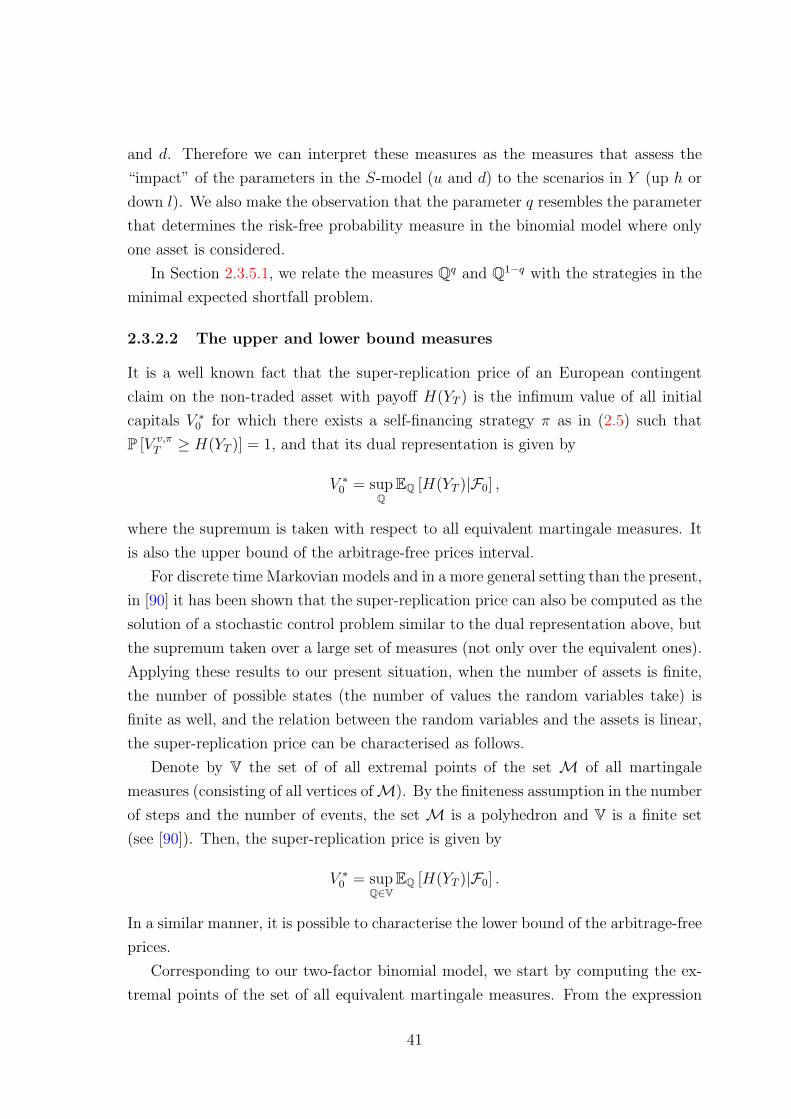
and d. Therefore we can interpret these measures as the measures that assess the
“impact” of the parameters in the S-model (u and d) to the scenarios in Y (up h or
down l). We also make the observation that the parameter q resembles the parameter
that determines the risk-free probability measure in the binomial model where only
one asset is considered.
In Section 2.3.5.1, we relate the measures Qq and Q1−q with the strategies in the
minimal expected shortfall problem.
2.3.2.2 The upper and lower bound measures
It is a well known fact that the super-replication price of an European contingent
claim on the non-traded asset with payoff H(YT ) is the infimum value of all initial
capitals V ∗0 for which there exists a self-financing strategy π as in (2.5) such that
P [V v,πT ≥ H(YT )] = 1, and that its dual representation is given by
V ∗0 = sup
QEQ [H(YT )|F0] ,
where the supremum is taken with respect to all equivalent martingale measures. It
is also the upper bound of the arbitrage-free prices interval.
For discrete time Markovian models and in a more general setting than the present,
in [90] it has been shown that the super-replication price can also be computed as the
solution of a stochastic control problem similar to the dual representation above, but
the supremum taken over a large set of measures (not only over the equivalent ones).
Applying these results to our present situation, when the number of assets is finite,
the number of possible states (the number of values the random variables take) is
finite as well, and the relation between the random variables and the assets is linear,
the super-replication price can be characterised as follows.
Denote by V the set of of all extremal points of the set M of all martingale
measures (consisting of all vertices ofM). By the finiteness assumption in the number
of steps and the number of events, the set M is a polyhedron and V is a finite set
(see [90]). Then, the super-replication price is given by
V ∗0 = sup
Q∈VEQ [H(YT )|F0] .
In a similar manner, it is possible to characterise the lower bound of the arbitrage-free
prices.
Corresponding to our two-factor binomial model, we start by computing the ex-
tremal points of the set of all equivalent martingale measures. From the expression
41
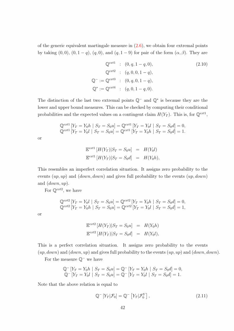
of the generic equivalent martingale measure in (2.6), we obtain four extremal points
by taking (0, 0), (0, 1− q), (q, 0), and (q, 1− 9) for pair of the form (α, β). They are
Qext1 : (0, q, 1− q, 0), (2.10)
Qext2 : (q, 0, 0, 1− q),
Q− := Qext3 : (0, q, 0, 1− q),
Q∗ := Qext4 : (q, 0, 1− q, 0).
The distinction of the last two extremal points Q− and Q∗ is because they are the
lower and upper bound measures. This can be checked by computing their conditional
probabilities and the expected values on a contingent claim H(YT ). This is, for Qext1,
Qext1 [YT = Y0h | ST = S0u] = Qext1 [YT = Y0l | ST = S0d] = 0,Qext1 [YT = Y0l | ST = S0u] = Qext1 [YT = Y0h | ST = S0d] = 1.
or
Eext1 [H(YT )|ST = S0u] = H(Y0l)
Eext1 [H(YT )|ST = S0d] = H(Y0h),
This resembles an imperfect correlation situation. It assigns zero probability to the
events (up, up) and (down, down) and gives full probability to the events (up, down)
and (down, up).
For Qext2, we have
Qext2 [YT = Y0l | ST = S0u] = Qext2 [YT = Y0h | ST = S0d] = 0,Qext2 [YT = Y0h | ST = S0u] = Qext2 [YT = Y0l | ST = S0d] = 1,
or
Eext2 [H(YT )|ST = S0u] = H(Y0h)
Eext2 [H(YT )|ST = S0d] = H(Y0l),
This is a perfect correlation situation. It assigns zero probability to the events
(up, down) and (down, up) and gives full probability to the events (up, up) and (down, down).
For the measure Q− we have
Q− [YT = Y0h | ST = S0u] = Q− [YT = Y0h | ST = S0d] = 0,Q− [YT = Y0l | ST = S0u] = Q− [YT = Y0l | ST = S0d] = 1.
Note that the above relation is equal to
Q− [YT |F0] = Q− [YT |FY0
], (2.11)
42
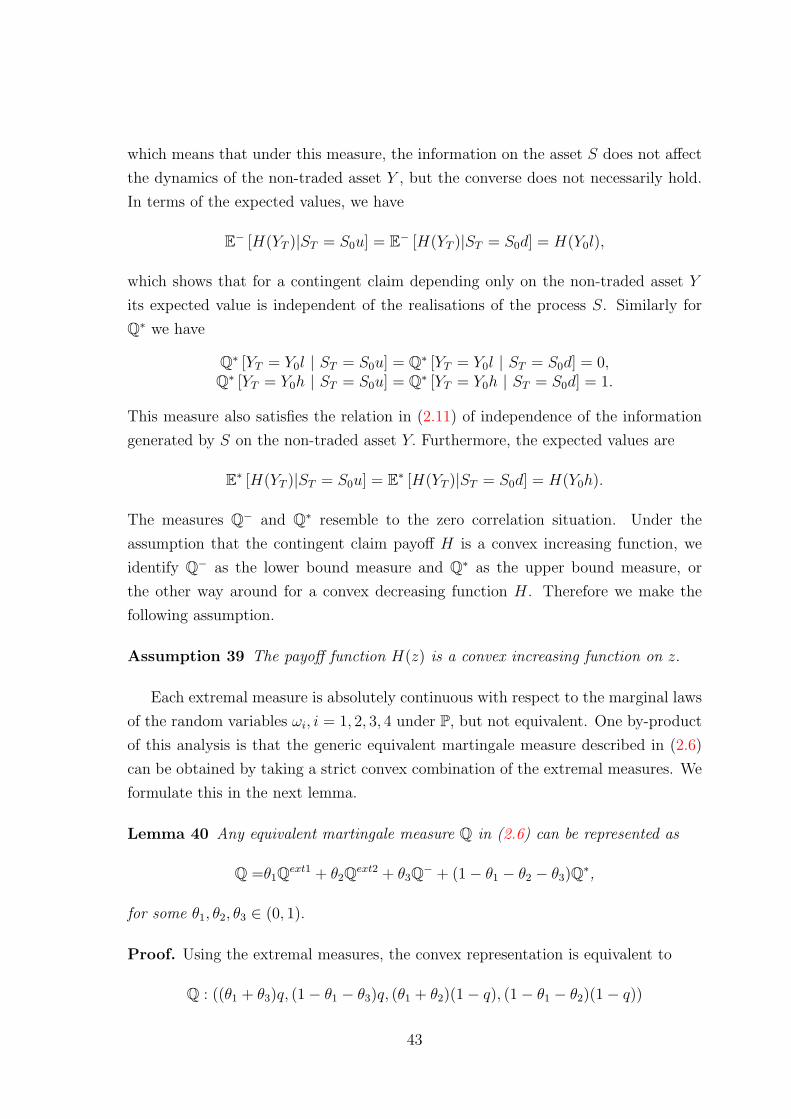
which means that under this measure, the information on the asset S does not affect
the dynamics of the non-traded asset Y , but the converse does not necessarily hold.
In terms of the expected values, we have
E− [H(YT )|ST = S0u] = E− [H(YT )|ST = S0d] = H(Y0l),
which shows that for a contingent claim depending only on the non-traded asset Y
its expected value is independent of the realisations of the process S. Similarly for
Q∗ we have
Q∗ [YT = Y0l | ST = S0u] = Q∗ [YT = Y0l | ST = S0d] = 0,Q∗ [YT = Y0h | ST = S0u] = Q∗ [YT = Y0h | ST = S0d] = 1.
This measure also satisfies the relation in (2.11) of independence of the information
generated by S on the non-traded asset Y. Furthermore, the expected values are
E∗ [H(YT )|ST = S0u] = E∗ [H(YT )|ST = S0d] = H(Y0h).
The measures Q− and Q∗ resemble to the zero correlation situation. Under the
assumption that the contingent claim payoff H is a convex increasing function, we
identify Q− as the lower bound measure and Q∗ as the upper bound measure, or
the other way around for a convex decreasing function H. Therefore we make the
following assumption.
Assumption 39 The payoff function H(z) is a convex increasing function on z.
Each extremal measure is absolutely continuous with respect to the marginal laws
of the random variables ωi, i = 1, 2, 3, 4 under P, but not equivalent. One by-product
of this analysis is that the generic equivalent martingale measure described in (2.6)
can be obtained by taking a strict convex combination of the extremal measures. We
formulate this in the next lemma.
Lemma 40 Any equivalent martingale measure Q in (2.6) can be represented as
Q =θ1Qext1 + θ2Qext2 + θ3Q− + (1− θ1 − θ2 − θ3)Q∗,
for some θ1, θ2, θ3 ∈ (0, 1).
Proof. Using the extremal measures, the convex representation is equivalent to
Q : ((θ1 + θ3)q, (1− θ1 − θ3)q, (θ1 + θ2)(1− q), (1− θ1 − θ2)(1− q))
43
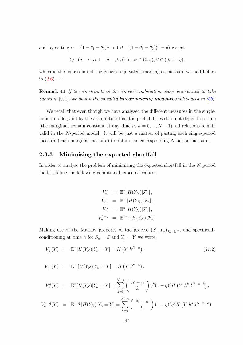
and by setting α = (1− θ1 − θ3)q and β = (1− θ1 − θ2)(1− q) we get
Q : (q − α, α, 1− q − β, β) for α ∈ (0, q), β ∈ (0, 1− q),
which is the expression of the generic equivalent martingale measure we had before
in (2.6).
Remark 41 If the constraints in the convex combination above are relaxed to take
values in [0, 1], we obtain the so called linear pricing measures introduced in [69].
We recall that even though we have analysed the different measures in the single-
period model, and by the assumption that the probabilities does not depend on time
(the marginals remain constant at any time n, n = 0, ..., N − 1), all relations remain
valid in the N -period model. It will be just a matter of pasting each single-period
measure (each marginal measure) to obtain the corresponding N -period measure.
2.3.3 Minimising the expected shortfall
In order to analyse the problem of minimising the expected shortfall in the N -period
model, define the following conditional expected values:
V ∗n = E∗ [H(YN)|Fn] ,
V −n = E− [H(YN)|Fn] ,
V qn = Eq [H(YN)|Fn] ,
V 1−qn = E1−q [H(YN)|Fn] .
Making use of the Markov property of the process (Sn, Yn)0≤n≤N , and specifically
conditioning at time n for Sn = S and Yn = Y we write,
V ∗n (Y ) = E∗ [H(YN)|Yn = Y ] = H
(Y hN−n
), (2.12)
V −n (Y ) = E− [H(YN)|Yn = Y ] = H
(Y lN−n
),
V qn (Y ) = Eq [H(YN)|Yn = Y ] =
N−n∑k=0
(N − nk
)qk(1− q)kH
(Y hk lN−n−k
),
V 1−qn (Y ) = E1−q [H(YN)|Yn = Y ] =
N−n∑k=0
(N − nk
)(1− q)kqkH
(Y hk lN−n−k
).
44
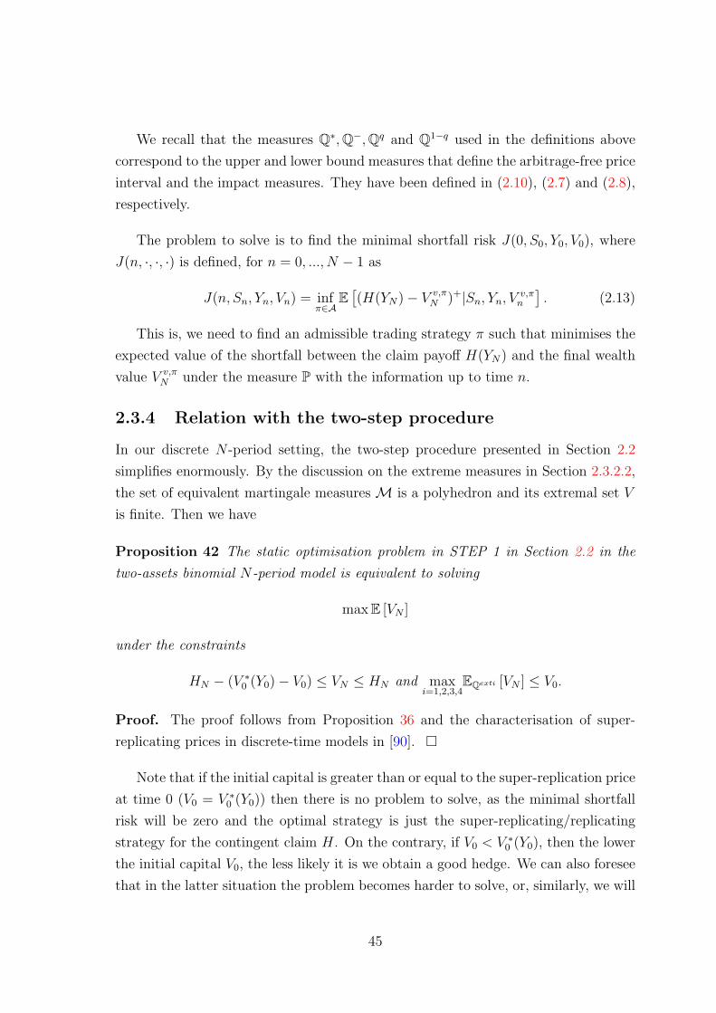
We recall that the measures Q∗,Q−,Qq and Q1−q used in the definitions above
correspond to the upper and lower bound measures that define the arbitrage-free price
interval and the impact measures. They have been defined in (2.10), (2.7) and (2.8),
respectively.
The problem to solve is to find the minimal shortfall risk J(0, S0, Y0, V0), where
J(n, ·, ·, ·) is defined, for n = 0, ..., N − 1 as
J(n, Sn, Yn, Vn) = infπ∈A
E[(H(YN)− V v,π
N )+|Sn, Yn, Vv,πn
]. (2.13)
This is, we need to find an admissible trading strategy π such that minimises the
expected value of the shortfall between the claim payoff H(YN) and the final wealth
value V v,πN under the measure P with the information up to time n.
2.3.4 Relation with the two-step procedure
In our discrete N -period setting, the two-step procedure presented in Section 2.2
simplifies enormously. By the discussion on the extreme measures in Section 2.3.2.2,
the set of equivalent martingale measures M is a polyhedron and its extremal set V
is finite. Then we have
Proposition 42 The static optimisation problem in STEP 1 in Section 2.2 in the
two-assets binomial N-period model is equivalent to solving
max E [VN ]
under the constraints
HN − (V ∗0 (Y0)− V0) ≤ VN ≤ HN and max
i=1,2,3,4EQexti [VN ] ≤ V0.
Proof. The proof follows from Proposition 36 and the characterisation of super-
replicating prices in discrete-time models in [90].
Note that if the initial capital is greater than or equal to the super-replication price
at time 0 (V0 = V ∗0 (Y0)) then there is no problem to solve, as the minimal shortfall
risk will be zero and the optimal strategy is just the super-replicating/replicating
strategy for the contingent claim H. On the contrary, if V0 < V ∗0 (Y0), then the lower
the initial capital V0, the less likely it is we obtain a good hedge. We can also foresee
that in the latter situation the problem becomes harder to solve, or, similarly, we will
45
need more conditions to check in order to find the minimal shortfall and the optimal
strategy.
Although Proposition 42 suggests the general algorithm for calculating the mini-
mal expected shortfall, it involves solving at each time n = 0, ..., N−1 a discrete-time
constrained stochastic control problem. Instead, we take a more direct approach by
looking at the original formulation.
There are three main cases to analyse regarding the initial capital V0. They are
linked to the strategies, the impact and extreme measures as explained in the next
section.
2.3.5 The single-period model
2.3.5.1 The strategies, the impact and the extreme measures
In this section, we relate the strategies (optimal strategies and candidate strategies)
to the impact and extreme measures.
The key aspect in the solution to the problem in (2.13) of minimising the expected
shortfall is to exploit the Markov property of the process (Sn, Yn)0≤n≤N and make use
of the Dynamic Programming Principle (see [6]) to solve via backward induction. At
each step N −1, the goal is to find the minimum and the minimiser π in the equation
J(N − 1, SN−1, YN−1, VN−1) = infπ
E[(H(YN)− VN)+|SN−1, YN−1, VN−1
].
Using the expression for the portfolio dynamics in (2.5) and assigning the corre-
sponding probabilities to each of the four possible scenarios, the problem reduces to
find at the step N − 1 the value π that minimises the function f defined by
f(π) = p1 [H(YN−1h)− VN−1 − πSN−1(u− 1)]+ (2.14)
+p2 [H(YN−1l)− VN−1 − πSN−1(u− 1)]+
+p3 [H(YN−1h)− VN−1 − πSN−1(d− 1)]+
+p4 [H(YN−1l)− VN−1 − πSN−1(d− 1)]+ .
As is customary in these situations, in order to search for the minimiser of f , we start
by defining four candidates for optimal strategies by making each term of the above
sum in (2.14) equal to zero. The four candidates to optimal strategies are:
πuh := H(YN−1h)−VN−1
SN−1(u−1), πul := H(YN−1l)−VN−1
SN−1(u−1),
πdh := H(YN−1h)−VN−1
SN−1(d−1), πdh := H(YN−1l)−VN−1
SN−1(d−1).
(2.15)
46
If by Assumption 39 the payoff function H is a convex increasing function on Y ,
and by the expressions of the candidate strategies in (2.15) we obtain the following
relations:
πuh > πul; πdl > πdh;q − 1
qπuh = πdh and
q − 1
qπul = πdl.
Furthermore, also by the convexity and increasing property of H we have for any π
H(YN−1l)− VN−1 − πSN−1(d− 1) < H(YN−1h)− VN−1 − πSN−1(d− 1),
H(YN−1l)− VN−1 − πSN−1(u− 1) < H(YN−1h)− VN−1 − πSN−1(u− 1).
This helps to simplify the expressions for f in (2.14) in each of the four candidate
strategies, yielding
f(πuh) =p3
1− q
[V ∗
N−1(YN−1)− VN−1
]++
p4
1− q
[V q
N−1(YN−1)− VN−1
]+, (2.16)
f(πdh) =p1
q
[V ∗
N−1(YN−1)− VN−1
]++p2
q
[V 1−q
N−1(YN−1)− VN−1
]+,
f(πdl) =p1
q
[V q
N−1(YN−1)− VN−1
]++p2
q
[V −
N−1(YN−1)− VN−1
]++p3
[V ∗
N−1(YN−1)− V −N−1(YN−1)
]+,
f(πul) = p1
[V ∗
N−1(YN−1)− V −N−1(YN−1)
]++
p3
1− q
[V 1−q
N−1(YN−1)− VN−1
]++
p4
1− q
[V −
N−1(YN−1)− VN−1
]+.
We are now in the position to relate the candidate strategies to the impact mea-
sures. Define e1 and e2 as the difference between the expected value of the claim H
under the measure Qq (resp. Q1−q) conditional to the information up to time N − 1
and the wealth value at time N − 1, this is,
e1 := V qN−1(YN−1)− VN−1
e2 := V 1−qN−1(YN−1)− VN−1.
Using the expressions of the candidate strategies in (2.15), the definition of the
impact measures in (2.7) and (2.8), and after some algebra we have the following
47
relations.
e1 = qH(YN−1h) + (1− q)H(YN−1l)− VN−1 (2.17)
=(u− 1)(1− d)
u− dSN−1
(πuh − πdl
),
e2 = (1− q)H(YN−1h) + qH(YN−1l)− VN−1
=(u− 1)(1− d)
u− dSN−1
(πul − πdh
).
The quantity e1 involves only the parameters u, d, SN−1 and the difference between
the candidate strategies πuh − πdl. As 0 < d < 1 < u and SN−1 > 0, then the sign in
e1 depends on whether πuh is bigger than πdl or not. Similarly for e2, its sign depends
on the values of πuland πdh.
These relations between e1 and e2 highlights the importance of the parameter q
in the decision of optimal strategy and optimal solution.
To see a more clear interpretation, define for a generic martingale measure Q as
in (2.6) the functions:
u(α) := EQ [H(YT )|SN = SN−1u] (2.18)
=q − α
qH(YN−1h) +
α
qH(YN−1l), (2.19)
w(β) := EQ [H(YT )|SN = SN−1d] (2.20)
=1− q − β
1− qH(YN−1h) +
β
1− qH(YN−1l). (2.21)
Both of this functions are decreasing in α and β, with
u(0) = H(YN−1h), u(q) = H(YN−1l), w(0) = H(YN−1h) and w(1−q) = H(YN−1l).
On the other hand, for q ∈ [0, 1] the following inequalities always hold, (see Figure
2.1):
if 0 ≤ q < 3−√
52
then 1− q ≥ (1− q)2 > q ≥ q(1− q) ≥ q2,
if 3−√
52
≤ q < 12
then 1− q > (1− q)2 ≥ q > q(1− q) > q2,
if q = 12
then 1− q = q > (1− q)2 = q(1− q) = q2,
if 12< q ≤ −1+
√5
2then q > 1− q ≥ q2 > q(1− q) > (1− q)2,
if −1+√
52
< q ≤ 1 then q ≥ q2 > 1− q ≥ q(1− q) ≥ (1− q)2.
48
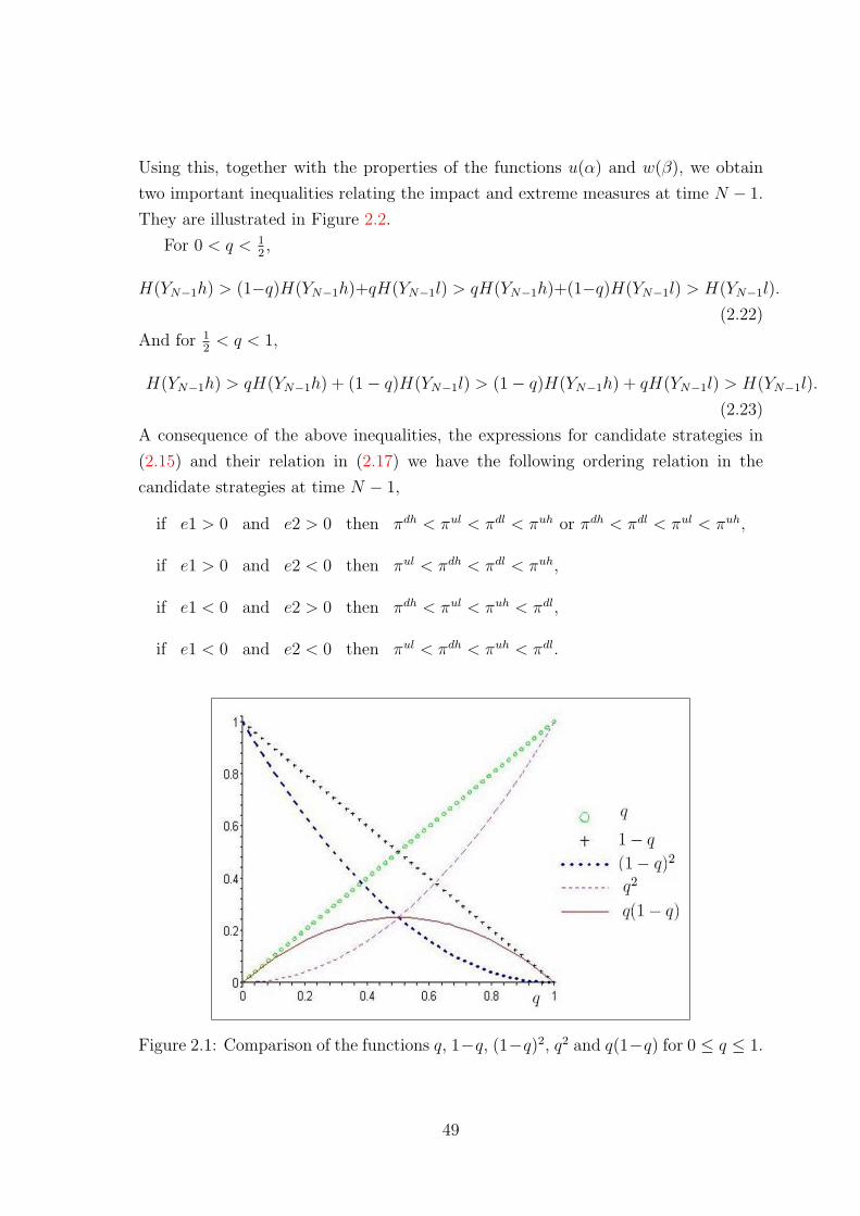
Using this, together with the properties of the functions u(α) and w(β), we obtain
two important inequalities relating the impact and extreme measures at time N − 1.
They are illustrated in Figure 2.2.
For 0 < q < 12,
H(YN−1h) > (1−q)H(YN−1h)+qH(YN−1l) > qH(YN−1h)+(1−q)H(YN−1l) > H(YN−1l).
(2.22)
And for 12< q < 1,
H(YN−1h) > qH(YN−1h) + (1− q)H(YN−1l) > (1− q)H(YN−1h) + qH(YN−1l) > H(YN−1l).
(2.23)
A consequence of the above inequalities, the expressions for candidate strategies in
(2.15) and their relation in (2.17) we have the following ordering relation in the
candidate strategies at time N − 1,
if e1 > 0 and e2 > 0 then πdh < πul < πdl < πuh or πdh < πdl < πul < πuh,
if e1 > 0 and e2 < 0 then πul < πdh < πdl < πuh,
if e1 < 0 and e2 > 0 then πdh < πul < πuh < πdl,
if e1 < 0 and e2 < 0 then πul < πdh < πuh < πdl.
Figure 2.1: Comparison of the functions q, 1−q, (1−q)2, q2 and q(1−q) for 0 ≤ q ≤ 1.
49
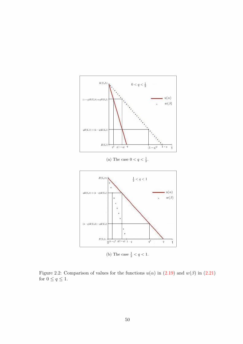
(a) The case 0 < q < 12 .
(b) The case 12 < q < 1.
Figure 2.2: Comparison of values for the functions u(α) in (2.19) and w(β) in (2.21)for 0 ≤ q ≤ 1.
50
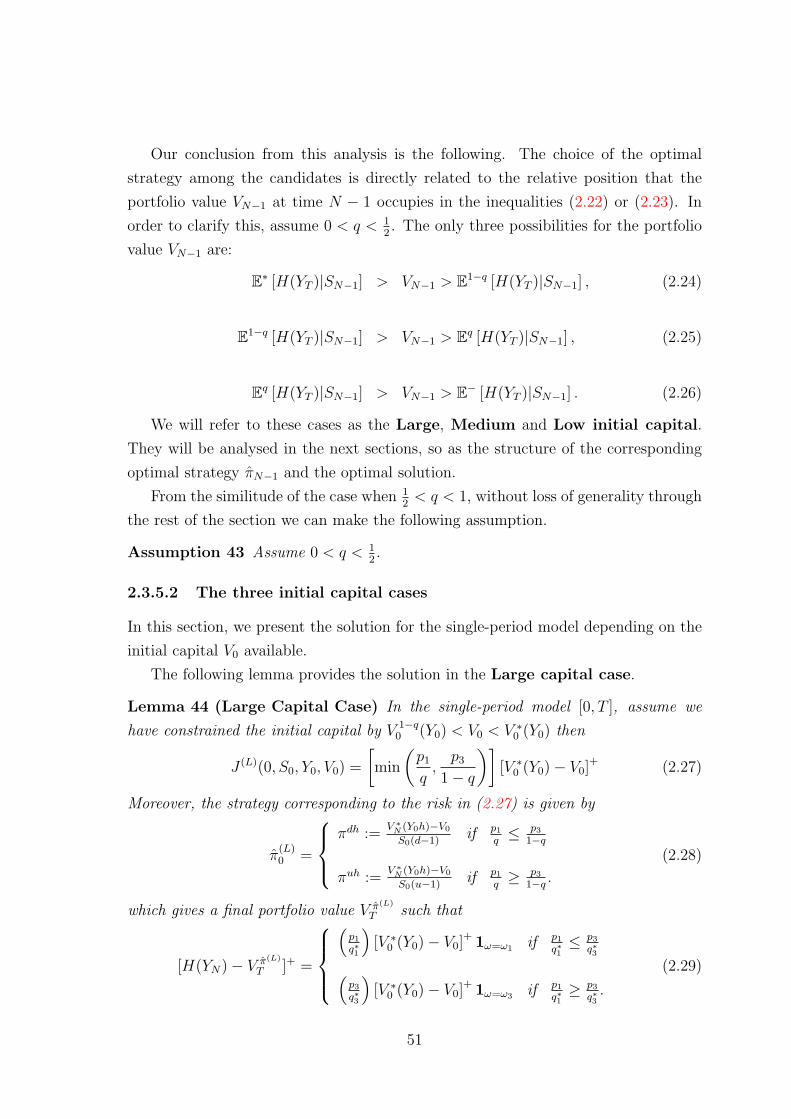
Our conclusion from this analysis is the following. The choice of the optimal
strategy among the candidates is directly related to the relative position that the
portfolio value VN−1 at time N − 1 occupies in the inequalities (2.22) or (2.23). In
order to clarify this, assume 0 < q < 12. The only three possibilities for the portfolio
value VN−1 are:
E∗ [H(YT )|SN−1] > VN−1 > E1−q [H(YT )|SN−1] , (2.24)
E1−q [H(YT )|SN−1] > VN−1 > Eq [H(YT )|SN−1] , (2.25)
Eq [H(YT )|SN−1] > VN−1 > E− [H(YT )|SN−1] . (2.26)
We will refer to these cases as the Large, Medium and Low initial capital.
They will be analysed in the next sections, so as the structure of the corresponding
optimal strategy πN−1 and the optimal solution.
From the similitude of the case when 12< q < 1, without loss of generality through
the rest of the section we can make the following assumption.
Assumption 43 Assume 0 < q < 12.
2.3.5.2 The three initial capital cases
In this section, we present the solution for the single-period model depending on the
initial capital V0 available.
The following lemma provides the solution in the Large capital case.
Lemma 44 (Large Capital Case) In the single-period model [0, T ], assume we
have constrained the initial capital by V 1−q0 (Y0) < V0 < V ∗
0 (Y0) then
J (L)(0, S0, Y0, V0) =
[min
(p1
q,p3
1− q
)][V ∗
0 (Y0)− V0]+ (2.27)
Moreover, the strategy corresponding to the risk in (2.27) is given by
π(L)0 =
πdh :=
V ∗N (Y0h)−V0
S0(d−1)if p1
q≤ p3
1−q
πuh :=V ∗
N (Y0h)−V0
S0(u−1)if p1
q≥ p3
1−q.
(2.28)
which gives a final portfolio value V π(L)
T such that
[H(YN)− V π(L)
T ]+ =
(
p1
q∗1
)[V ∗
0 (Y0)− V0]+ 1ω=ω1 if p1
q∗1≤ p3
q∗3(p3
q∗3
)[V ∗
0 (Y0)− V0]+ 1ω=ω3 if p1
q∗1≥ p3
q∗3.
(2.29)
51
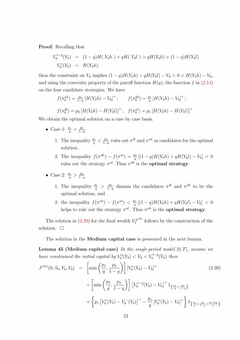
Proof. Recalling that
V 1−q0 (Y0) = (1− q)H( Y0h ) + qH( Y0l ) > qH(Y0h) + (1− q)H(Y0l)
V ∗0 (Y0) = H(Y0h),
then the constraint on V0 implies (1− q)H(Y0h) + qH(Y0l)− V0 < 0 < H(Y0h)− V0,
and using the convexity property of the payoff function H(y), the function f in (2.14)
on the four candidate strategies. We have
f(πuh0 ) = p3
1−q[H(Y0h)− V0]
+ ; f(πdh0 ) = p1
q[H(Y0h)− V0]
+ ;
f(πdl0 ) = p3 [H(Y0h)−H(Y0l)]
+ ; f(πul0 ) = p1 [H(Y0h)−H(Y0l)]
+ .
We obtain the optimal solution on a case by case basis.
• Case 1: p1
q< p3
1−q.
1. The inequality p1
q< p3
1−qrules out πdl and πuh as candidates for the optimal
solution.
2. The inequality f(πdh) − f(πul) = p1
q[(1− q)H(Y0h) + qH(Y0l)− V0] < 0
rules out the strategy πul. Thus πdh is the optimal strategy.
• Case 2: p1
q> p3
1−q
1. The inequality p1
q> p3
1−qdismiss the candidates πdl and πdh to be the
optimal solution, and
2. the inequality f(πuh) − f(πul) < p1
q[(1− q)H(Y0h) + qH(Y0l)− V0] < 0
helps to rule out the strategy πul. Thus πuh is the optimal strategy.
The relation in (2.29) for the final wealth V π(H)
T follows by the construction of the
solution.
The solution in the Medium capital case is presented in the next lemma.
Lemma 45 (Medium capital case) In the single-period model [0, T ], assume we
have constrained the initial capital by V q0 (Y0) < V0 < V 1−q
0 (Y0) then
J (M)(0, S0, Y0, V0) =
[min
(p1
q,p3
1− q
)][V ∗
0 (Y0)− V0]+ (2.30)
+
[min
(p2
q,p3
1− q
)] [V 1−q
0 (Y0)− V0
]+1 p1
q<
p31−q
+
p1
[V ∗
0 (Y0)− V −0 (Y0)
]+ − p1
q[V ∗
0 (Y0)− V0]+
1 p1
q<
p31−q
<p1+p2
q
52
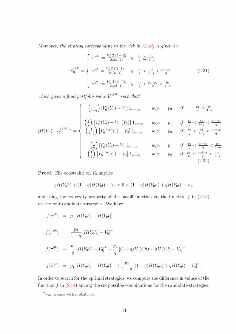
Moreover, the strategy corresponding to the risk in (2.30) is given by
π(M)0 =
πuh :=V ∗
N (Y0h)−V0
S0(u−1)if p1
q≥ p3
1−q
πul :=V ∗
N (Y0l)−V0
S0(u−1)if p1
q< p3
1−q< p1+p2
q
πdh :=V ∗
N (Y0h)−V0
S0(d−1)if p1
q< p1+p2
q< p3
1−q.
. (2.31)
which gives a final portfolio value V π(M)
T such that2
[H(YT )−V π(M)
T ]+ =
(1
1−q
)[V ∗
0 (Y0)− V0]1ω=ω3 w.p. p3 if p1
q≥ p3
1−q(1q
) [V ∗
0 (Y0)− V −0 (Y0)
]1ω=ω1 w.p. p1 if p1
q< p3
1−q< p1+p2
q(1
1−q
) [V 1−q
0 (Y0)− V0
]1ω=ω3 w.p. p3 if p1
q< p3
1−q< p1+p2
q(1q
)[V ∗
0 (Y0)− V0]1ω=ω1 w.p. p1 if p1
q< p1+p2
q< p3
1−q(1q
) [V 1−q
0 (Y0)− V0
]1ω=ω2 w.p. p2 if p1
q< p1+p2
q< p3
1−q.
(2.32)
Proof. The constraint on V0 implies
qH(Y0h) + (1− q)H(Y0l)− V0 < 0 < (1− q)H(Y0h) + qH(Y0l)− V0,
and using the convexity property of the payoff function H, the function f in (2.14)
on the four candidate strategies. We have
f(πdl) = p3 [H(Y0h)−H(Y0l)]+
f(πuh) =p3
1− q[H(Y0h)− V0]
+
f(πdh) =p1
q[H(Y0h)− V0]
+ +p2
q[(1− q)H(Y0h) + qH(Y0l)− V0]
+
f(πul) = p1 [H(Y0h)−H(Y0l)]+ +
p3
1− q[(1− q)H(Y0h) + qH(Y0l)− V0]
+ .
In order to search for the optimal strategies, we compute the difference in values of the
function f in (2.14) among the six possible combinations for the candidate strategies.
2w.p. means with probability.
53
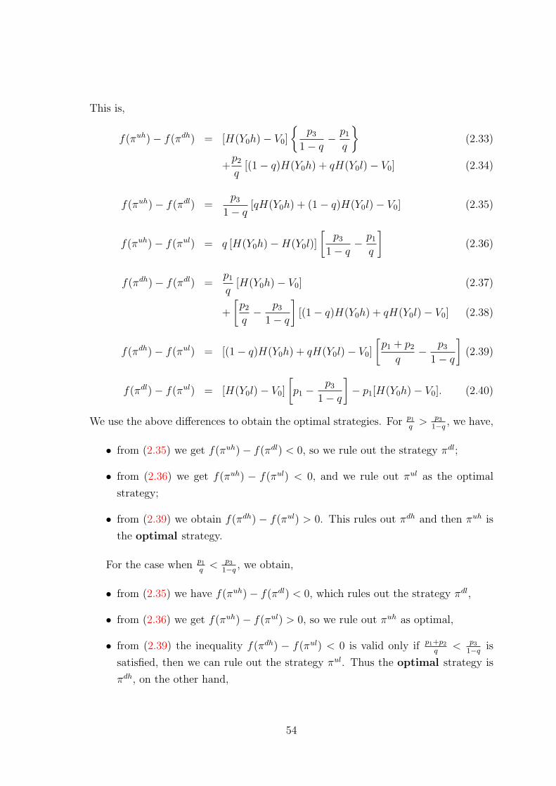
This is,
f(πuh)− f(πdh) = [H(Y0h)− V0]
p3
1− q− p1
q
(2.33)
+p2
q[(1− q)H(Y0h) + qH(Y0l)− V0] (2.34)
f(πuh)− f(πdl) =p3
1− q[qH(Y0h) + (1− q)H(Y0l)− V0] (2.35)
f(πuh)− f(πul) = q [H(Y0h)−H(Y0l)]
[p3
1− q− p1
q
](2.36)
f(πdh)− f(πdl) =p1
q[H(Y0h)− V0] (2.37)
+
[p2
q− p3
1− q
][(1− q)H(Y0h) + qH(Y0l)− V0] (2.38)
f(πdh)− f(πul) = [(1− q)H(Y0h) + qH(Y0l)− V0]
[p1 + p2
q− p3
1− q
](2.39)
f(πdl)− f(πul) = [H(Y0l)− V0]
[p1 −
p3
1− q
]− p1[H(Y0h)− V0]. (2.40)
We use the above differences to obtain the optimal strategies. For p1
q> p3
1−q, we have,
• from (2.35) we get f(πuh)− f(πdl) < 0, so we rule out the strategy πdl;
• from (2.36) we get f(πuh) − f(πul) < 0, and we rule out πul as the optimal
strategy;
• from (2.39) we obtain f(πdh) − f(πul) > 0. This rules out πdh and then πuh is
the optimal strategy.
For the case when p1
q< p3
1−q, we obtain,
• from (2.35) we have f(πuh)− f(πdl) < 0, which rules out the strategy πdl,
• from (2.36) we get f(πuh)− f(πul) > 0, so we rule out πuh as optimal,
• from (2.39) the inequality f(πdh) − f(πul) < 0 is valid only if p1+p2
q< p3
1−qis
satisfied, then we can rule out the strategy πul. Thus the optimal strategy is
πdh, on the other hand,
54
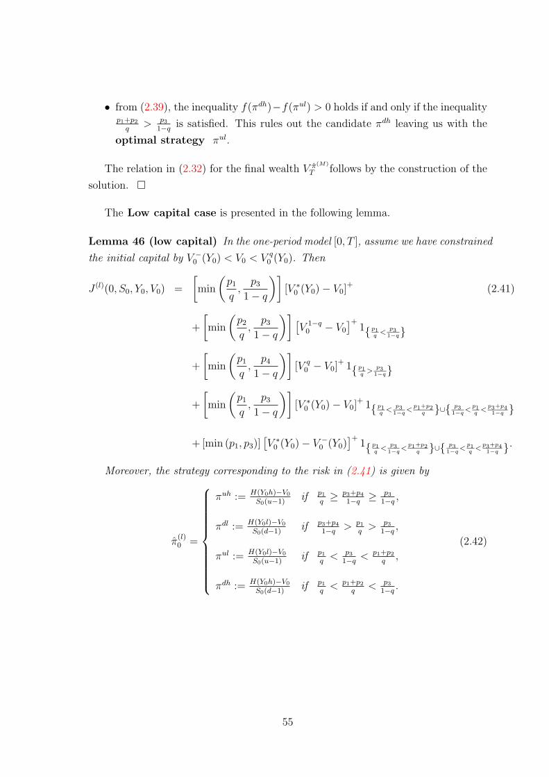
• from (2.39), the inequality f(πdh)−f(πul) > 0 holds if and only if the inequalityp1+p2
q> p3
1−qis satisfied. This rules out the candidate πdh leaving us with the
optimal strategy πul.
The relation in (2.32) for the final wealth V π(M)
T follows by the construction of the
solution.
The Low capital case is presented in the following lemma.
Lemma 46 (low capital) In the one-period model [0, T ], assume we have constrained
the initial capital by V −0 (Y0) < V0 < V q
0 (Y0). Then
J (l)(0, S0, Y0, V0) =
[min
(p1
q,p3
1− q
)][V ∗
0 (Y0)− V0]+ (2.41)
+
[min
(p2
q,p3
1− q
)] [V 1−q
0 − V0
]+1 p1
q<
p31−q
+
[min
(p1
q,p4
1− q
)][V q
0 − V0]+ 1 p1
q>
p31−q
+
[min
(p1
q,p3
1− q
)][V ∗
0 (Y0)− V0]+ 1 p1
q<
p31−q
<p1+p2
q ∪ p31−q
<p1q
<p3+p41−q
+ [min (p1, p3)][V ∗
0 (Y0)− V −0 (Y0)
]+1 p1
q<
p31−q
<p1+p2
q ∪ p31−q
<p1q
<p3+p41−q .
Moreover, the strategy corresponding to the risk in (2.41) is given by
π(l)0 =
πuh := H(Y0h)−V0
S0(u−1)if p1
q≥ p3+p4
1−q≥ p3
1−q,
πdl := H(Y0l)−V0
S0(d−1)if p3+p4
1−q> p1
q> p3
1−q,
πul := H(Y0l)−V0
S0(u−1)if p1
q< p3
1−q< p1+p2
q,
πdh := H(Y0h)−V0
S0(d−1)if p1
q< p1+p2
q< p3
1−q.
(2.42)
55
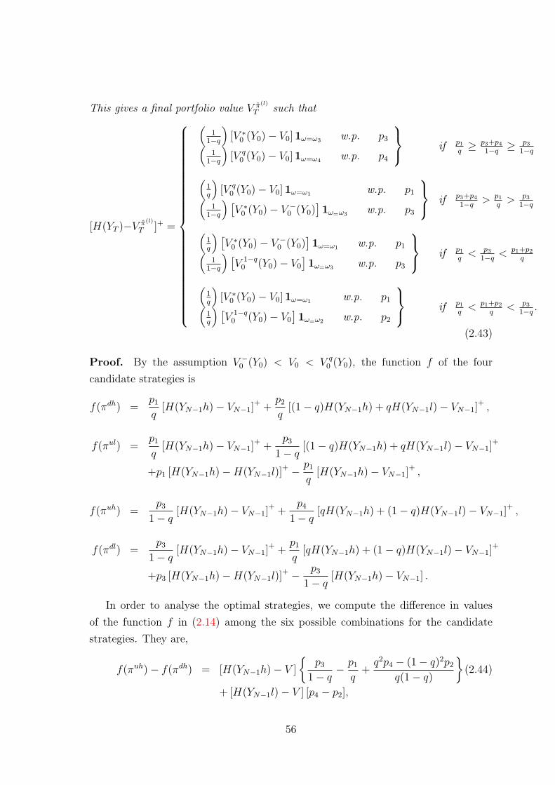
This gives a final portfolio value V π(l)
T such that
[H(YT )−V π(l)
T ]+ =
(1
1−q
)[V ∗
0 (Y0)− V0]1ω=ω3 w.p. p3(1
1−q
)[V q
0 (Y0)− V0]1ω=ω4 w.p. p4
if p1
q≥ p3+p4
1−q≥ p3
1−q
(1q
)[V q
0 (Y0)− V0]1ω=ω1 w.p. p1(1
1−q
) [V ∗
0 (Y0)− V −0 (Y0)
]1ω=ω3 w.p. p3
if p3+p4
1−q> p1
q> p3
1−q
(1q
) [V ∗
0 (Y0)− V −0 (Y0)
]1ω=ω1 w.p. p1(
11−q
) [V 1−q
0 (Y0)− V0
]1ω=ω3 w.p. p3
if p1
q< p3
1−q< p1+p2
q
(1q
)[V ∗
0 (Y0)− V0]1ω=ω1 w.p. p1(1q
) [V 1−q
0 (Y0)− V0
]1ω=ω2 w.p. p2
if p1
q< p1+p2
q< p3
1−q.
(2.43)
Proof. By the assumption V −0 (Y0) < V0 < V q
0 (Y0), the function f of the four
candidate strategies is
f(πdh) =p1
q[H(YN−1h)− VN−1]
+ +p2
q[(1− q)H(YN−1h) + qH(YN−1l)− VN−1]
+ ,
f(πul) =p1
q[H(YN−1h)− VN−1]
+ +p3
1− q[(1− q)H(YN−1h) + qH(YN−1l)− VN−1]
+
+p1 [H(YN−1h)−H(YN−1l)]+ − p1
q[H(YN−1h)− VN−1]
+ ,
f(πuh) =p3
1− q[H(YN−1h)− VN−1]
+ +p4
1− q[qH(YN−1h) + (1− q)H(YN−1l)− VN−1]
+ ,
f(πdl) =p3
1− q[H(YN−1h)− VN−1]
+ +p1
q[qH(YN−1h) + (1− q)H(YN−1l)− VN−1]
+
+p3 [H(YN−1h)−H(YN−1l)]+ − p3
1− q[H(YN−1h)− VN−1] .
In order to analyse the optimal strategies, we compute the difference in values
of the function f in (2.14) among the six possible combinations for the candidate
strategies. They are,
f(πuh)− f(πdh) = [H(YN−1h)− V ]
p3
1− q− p1
q+q2p4 − (1− q)2p2
q(1− q)
(2.44)
+ [H(YN−1l)− V ] [p4 − p2],
56
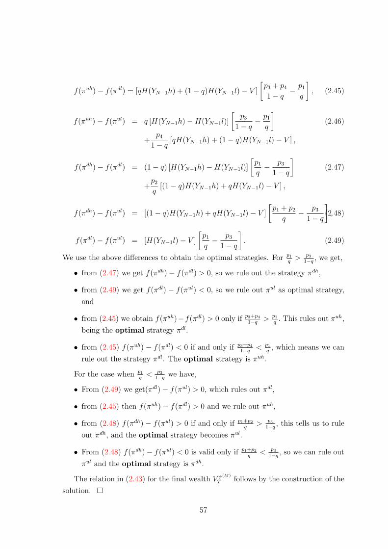
f(πuh)− f(πdl) = [qH(YN−1h) + (1− q)H(YN−1l)− V ]
[p3 + p4
1− q− p1
q
], (2.45)
f(πuh)− f(πul) = q [H(YN−1h)−H(YN−1l)]
[p3
1− q− p1
q
](2.46)
+p4
1− q[qH(YN−1h) + (1− q)H(YN−1l)− V ] ,
f(πdh)− f(πdl) = (1− q) [H(YN−1h)−H(YN−1l)]
[p1
q− p3
1− q
](2.47)
+p2
q[(1− q)H(YN−1h) + qH(YN−1l)− V ] ,
f(πdh)− f(πul) = [(1− q)H(YN−1h) + qH(YN−1l)− V ]
[p1 + p2
q− p3
1− q
],(2.48)
f(πdl)− f(πul) = [H(YN−1l)− V ]
[p1
q− p3
1− q
]. (2.49)
We use the above differences to obtain the optimal strategies. For p1
q> p3
1−q, we get,
• from (2.47) we get f(πdh)− f(πdl) > 0, so we rule out the strategy πdh,
• from (2.49) we get f(πdl) − f(πul) < 0, so we rule out πul as optimal strategy,
and
• from (2.45) we obtain f(πuh)−f(πdl) > 0 only if p3+p4
1−q> p1
q. This rules out πuh,
being the optimal strategy πdl.
• from (2.45) f(πuh)− f(πdl) < 0 if and only if p3+p4
1−q< p1
q, which means we can
rule out the strategy πdl. The optimal strategy is πuh.
For the case when p1
q< p3
1−qwe have,
• From (2.49) we get(πdl)− f(πul) > 0, which rules out πdl,
• from (2.45) then f(πuh)− f(πdl) > 0 and we rule out πuh,
• from (2.48) f(πdh) − f(πul) > 0 if and only if p1+p2
q> p3
1−q, this tells us to rule
out πdh, and the optimal strategy becomes πul.
• From (2.48) f(πdh)− f(πul) < 0 is valid only if p1+p2
q< p3
1−q, so we can rule out
πul and the optimal strategy is πdh.
The relation in (2.43) for the final wealth V π(M)
T follows by the construction of the
solution.
57
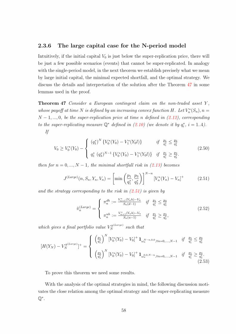
2.3.6 The large capital case for the N-period model
Intuitively, if the initial capital V0 is just below the super-replication price, there will
be just a few possible scenarios (events) that cannot be super-replicated. In analogy
with the single-period model, in the next theorem we establish precisely what we mean
by large initial capital, the minimal expected shortfall, and the optimal strategy. We
discuss the details and interpretation of the solution after the Theorem 47 in some
lemmas used in the proof.
Theorem 47 Consider a European contingent claim on the non-traded asset Y ,
whose payoff at time N is defined by an increasing convex function H. Let V ∗n (Sn), n =
N − 1, ..., 0, be the super-replication price at time n defined in (2.12), corresponding
to the super-replicating measure Q∗ defined in (2.10) (we denote it by q∗i , i = 1..4).
If
V0 ≥ V ∗0 (Y0)−
(q∗1)
N V ∗0 (Y0)− V ∗
1 (Y0l) if p1
q∗1≤ p3
q∗3
q∗1 (q∗3)N−1 V ∗
0 (Y0)− V ∗1 (Y0l) if p1
q∗1≥ p3
q∗3.
(2.50)
then for n = 0, ..., N − 1, the minimal shortfall risk in (2.13) becomes
J (Large)(n, Sn, Yn, Vn) =
[min
(p1
q∗1,p3
q∗3
)]N−n
[V ∗n (Yn)− Vn]+ (2.51)
and the strategy corresponding to the risk in (2.51) is given by
π(Large)n =
πdh
n :=V ∗
n+1(Ynh)−Vn
Sn(d−1)if p1
q∗1≤ p3
q∗3
πuhn :=
V ∗n+1(Ynh)−Vn
Sn(u−1)if p1
q∗1≥ p3
q∗3,
(2.52)
which gives a final portfolio value V π(Large)
N such that
[H(YN)− V π(Large)
N ]+ =
(
p1
q∗1
)N
[V ∗0 (Y0)− V0]
+ 1ωN−n,0,0n ,∀n=0,....,N−1 if p1
q∗1≤ p3
q∗3(p3
q∗3
)N
[V ∗0 (Y0)− V0]
+ 1ω0,0,N−nn ,∀n=0,....,N−1 if p1
q∗1≥ p3
q∗3.
(2.53)
To prove this theorem we need some results.
With the analysis of the optimal strategies in mind, the following discussion moti-
vates the close relation among the optimal strategy and the super-replicating measure
Q∗.
58
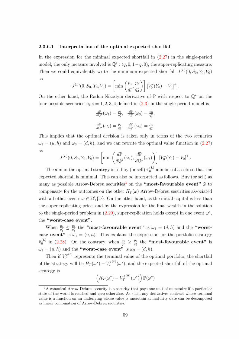
2.3.6.1 Interpretation of the optimal expected shortfall
In the expression for the minimal expected shortfall in (2.27) in the single-period
model, the only measure involved is Q∗ : (q, 0, 1−q, 0), the super-replicating measure.
Then we could equivalently write the minimum expected shortfall J (L)(0, S0, Y0, V0)
as
J (L)(0, S0, Y0, V0) =
[min
(p1
q∗1,p3
q∗3
)][V ∗
0 (Y0)− V0]+ .
On the other hand, the Radon-Nikodym derivative of P with respect to Q∗ on the
four possible scenarios ωi, i = 1, 2, 3, 4 defined in (2.3) in the single-period model is
dPdQ∗ (ω1) = p1
q∗1, dP
dQ∗ (ω3) = p3
q∗3,
dPdQ∗ (ω2) = p2
q∗2, dP
dQ∗ (ω4) = p4
q∗4.
This implies that the optimal decision is taken only in terms of the two scenarios
ω1 = (u, h) and ω3 = (d, h), and we can rewrite the optimal value function in (2.27)
as
J (L)(0, S0, Y0, V0) =
[min
(dPdQ∗ (ω1),
dPdQ∗ (ω3)
)][V ∗
0 (Y0)− V0]+ .
The aim in the optimal strategy is to buy (or sell) π(L)0 number of assets so that the
expected shortfall is minimal. This can also be interpreted as follows. Buy (or sell) as
many as possible Arrow-Debreu securities3 on the “most-favourable event” ω to
compensate for the outcomes on the other HT (ω) Arrow-Debreu securities associated
with all other events ω ∈ Ω\ω. On the other hand, as the initial capital is less than
the super-replicating price, and by the expression for the final wealth in the solution
to the single-period problem in (2.29), super-replication holds except in one event ω∗,
the “worst-case event”.
When p1
q∗1≤ p3
q∗3the “most-favourable event” is ω3 = (d, h) and the “worst-
case event” is ω1 = (u, h). This explains the expression for the portfolio strategy
π(L)0 in (2.28). On the contrary, when p1
q∗1≥ p3
q∗3the “most-favourable event” is
ω1 = (u, h) and the “worst-case event” is ω3 = (d, h).
Then if V π(L)
T represents the terminal value of the optimal portfolio, the shortfall
of the strategy will be HT (ω∗)− V π(L)
T (ω∗), and the expected shortfall of the optimal
strategy is (HT (ω∗)− V π(H)
T (ω∗))
P(ω∗)
3A canonical Arrow Debreu security is a security that pays one unit of numeraire if a particularstate of the world is reached and zero otherwise. As such, any derivatives contract whose terminalvalue is a function on an underlying whose value is uncertain at maturity date can be decomposedas linear combination of Arrow-Debreu securities.
59
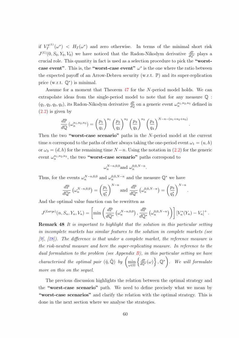
if V π(L)
T (ω∗) < HT (ω∗) and zero otherwise. In terms of the minimal short risk
J (L)(0, S0, Y0, V0) we have noticed that the Radon-Nikodym derivative dPdQ∗ plays a
crucial role. This quantity in fact is used as a selection procedure to pick the “worst-
case event”. This is, the “worst-case event” ω∗ is the one where the ratio between
the expected payoff of an Arrow-Debreu security (w.r.t. P) and its super-replication
price (w.r.t. Q∗) is minimal.
Assume for a moment that Theorem 47 for the N -period model holds. We can
extrapolate ideas from the single-period model to note that for any measure Q :
(q1, q2, q3, q4), its Radon-Nikodym derivative dPdQ on a generic event ωn1,n2,n3
n defined in
(2.2) is given by
dPdQ
(ωn1,n2,n3n ) =
(p1
q1
)n1(p2
q2
)n2(p3
q3
)n3(p4
q4
)N−n−(n1+n2+n3)
.
Then the two “worst-case scenario” paths in the N -period model at the current
time n correspond to the paths of either always taking the one-period event ω1 = (u, h)
or ω3 = (d, h) for the remaining time N−n. Using the notation in (2.2) for the generic
event ωn1,n2,n3n , the two “worst-case scenario” paths correspond to
ωN−n,0,0n and ω0,0,N−n
n .
Thus, for the events ωN−n,0,0n and ω0,0,N−n
n and the measure Q∗ we have
dPdQ∗
(ωN−n,0,0
n
)=
(p1
q∗1
)N−n
anddPdQ∗
(ω0,0,N−n
n
)=
(p3
q∗3
)N−n
.
And the optimal value function can be rewritten as
J (Large)(n, Sn, Yn, Vn) =
[min
(dPdQ∗
(ωN−n,0,0
n
),dPdQ∗
(ω0,0,N−n
n
))][V ∗
n (Yn)− Vn]+ .
Remark 48 It is important to highlight that the solution in this particular setting
in incomplete markets has similar features to the solution in complete markets (see
[9], [28]). The difference is that under a complete market, the reference measure is
the risk-neutral measure and here the super-replicating measure. In reference to the
dual formulation to the problem (see Appendix B), in this particular setting we have
characterised the optimal pair (η, Q) by
(minω∈Ω
dP
dQ∗ (ω),Q∗
). We will formulate
more on this on the sequel.
The previous discussion highlights the relation between the optimal strategy and
the “worst-case scenario” path. We need to define precisely what we mean by
“worst-case scenarios” and clarify the relation with the optimal strategy. This is
done in the next section where we analyse the strategies.
60
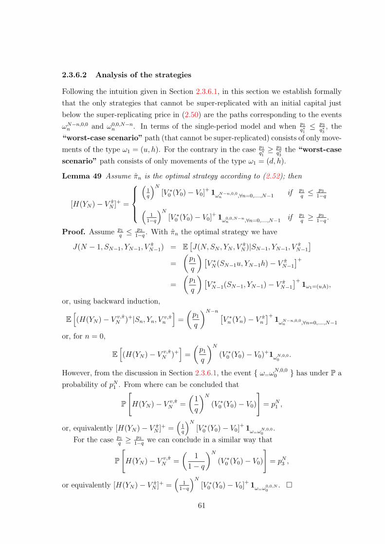
2.3.6.2 Analysis of the strategies
Following the intuition given in Section 2.3.6.1, in this section we establish formally
that the only strategies that cannot be super-replicated with an initial capital just
below the super-replicating price in (2.50) are the paths corresponding to the events
ωN−n,0,0n and ω0,0,N−n
n . In terms of the single-period model and when p1
q∗1≤ p3
q∗3, the
“worst-case scenario” path (that cannot be super-replicated) consists of only move-
ments of the type ω1 = (u, h). For the contrary in the case p1
q∗1≥ p3
q∗3the “worst-case
scenario” path consists of only movements of the type ω1 = (d, h).
Lemma 49 Assume πn is the optimal strategy according to (2.52); then
[H(YN)− V πN ]+ =
(
1q
)N
[V ∗0 (Y0)− V0]
+ 1ωN−n,0,0n ,∀n=0,....,N−1 if p1
q≤ p3
1−q(1
1−q
)N
[V ∗0 (Y0)− V0]
+ 1ω0,0,N−nn ,∀n=0,....,N−1 if p1
q≥ p3
1−q.
Proof. Assume p1
q≤ p3
1−q. With πn the optimal strategy we have
J(N − 1, SN−1, YN−1, VπN−1) = E
[J(N,SN , YN , V
πN )|SN−1, YN−1, V
πN−1
]=
(p1
q
)[V ∗
N(SN−1u, YN−1h)− V πN−1
]+=
(p1
q
)[V ∗
N−1(SN−1, YN−1)− V πN−1
]+1ω1=(u,h),
or, using backward induction,
E[(H(YN)− V v,π
N )+|Sn, Yn, Vv,πn
]=
(p1
q
)N−n [V ∗
n (Yn)− V πn
]+1ωN−n,0,0
n ,∀n=0,....,N−1
or, for n = 0,
E[(H(YN)− V v,π
N )+]
=
(p1
q
)N
(V ∗0 (Y0)− V0)
+1ωN,0,00
.
However, from the discussion in Section 2.3.6.1, the event ω=ωN,0,00 has under P a
probability of pN1 . From where can be concluded that
P
[H(YN)− V v,π
N =
(1
q
)N
(V ∗0 (Y0)− V0)
]= pN
1 ,
or, equivalently [H(YN)− V πN ]+ =
(1q
)N
[V ∗0 (Y0)− V0]
+ 1ω=ωN,0,00
.
For the case p1
q≥ p3
1−qwe can conclude in a similar way that
P
[H(YN)− V v,π
N =
(1
1− q
)N
(V ∗0 (Y0)− V0)
]= pN
3 ,
or equivalently [H(YN)− V πN ]+ =
(1
1−q
)N
[V ∗0 (Y0)− V0]
+ 1ω=ω0,0,N0
.
61
2.3.6.3 The initial capital condition
In this section, we formalise the relation between the condition (2.50) on the initial
capital V0 and a constraint on the optimal portfolio value V v,πn .
Lemma 50 If the inequality
V0 ≥ V ∗0 (Y0)−
(q∗1)
N V ∗1 (Y0h)− V ∗
1 (Y0l) if p1
q∗1≤ p3
q∗3
q∗1 (q∗3)N−1 V ∗
1 (Y0h)− V ∗1 (Y0l) if p1
q∗1≥ p3
q∗3
(2.54)
is satisfied, then
(1− q)V ∗n+1(Ynh) + qV ∗
n+1(Ynl) ≤ Vn
holds for all n = 0, .., N − 1.
Proof. The equality (1− q)V ∗n+1(Ynh) + qV ∗
n+1(Ynl) ≤ Vn is equivalent to
rn (V ∗n (Yn)− Vn) ≤ rnq
(V ∗
n (Yn)− V ∗n+1(Ynl)
)(2.55)
for r > 0 and for all n = 0, ..., N − 1. Assume p1
q≤ p3
1−qand using some intermediate
steps in the proof of Lemma 49 we have qn (V ∗n (Yn)− Vn) = V ∗
0 (Y0)− V01ω=ωN,0,00
.
Then for the relation (2.55) to be true we need the inequality V ∗0 (Y0)− V01ω=ωN,0,0
0≤
qn+1(V ∗
n (Yn)− V ∗n+1(Ynl)
)for all n = 0, ..., N − 1, or equivalently V ∗
0 (Y0)− V0 ≤qn+1
(V ∗
n (Y0 hn)− V ∗
n+1(Y0 hn l))
for all n = 0, . . . , N − 1. But this is equivalent to
(2.50) when p1
q≤ p3
1−q. For the remaining case when p1
q≥ p3
1−qwe proceed similarly us-
ing the relation (1−q)n (V ∗n (Yn)− Vn) = V ∗
0 (Y0)− V01ω=ω0,0,N0
to obtain the inequal-
ity V ∗0 (Y0)− V0 ≤ q(1 − q)n
(V ∗
n (Y0 hn)− V ∗
n+1(Y0 hn l))
for all n = 0, . . . , N − 1,
which give us the constraint in (2.50).
In the interpretation of the optimal strategy as buying/selling Arrow-Debreu secu-
rities, the condition on the initial capital (2.54) guarantees that this capital is enough
to buy/sell Arrow-Debreu securities on the most-favourable scenario events at every
time step n = 0, ..., N − 1.
When p1
q∗1≤ p3
q∗3the initial capital condition (2.54) can also be written as
V0 ≥ (1− qN)H(Y0hN) + qNH(Y0 l h
N−1) =: CL, (2.56)
and when p1
q∗1≤ p3
q∗3
V0 ≥ (1− q(1− q)N−1)H(Y0hN) + q(1− q)N−1H(Y0 l h
N−1) =: CL. (2.57)
62

This representation as a convex combination of the super-replicating price (H(Y0hN))
and a slightly lower level (H(Y0 l hN−1)) gives us the notion of how narrow the con-
dition on the initial capital is. Figure 2.3 shows the values for the condition CL and
the super-replication prices as function of the number of steps N for the numerical
parameters in Example 53. Furthermore, when N grows large, the condition be-
comes tighter meaning that the optimal strategy given by Theorem 47 is valid only
for initial capital values very close to the super-replication price. This is a very dis-
advantageous feature of the solution. It also represents problems if one would like to
obtain conclusions in the continuous-time by passing to the limit. This issue needs
further investigation and it is left to future research. Nevertheless, when the num-
ber of steps is not very large, it provides a manageable model and permits to get a
lot of insight on the solution in this particular incomplete market situation. This is
important as most of the incomplete market models are difficult to deal with.
Figure 2.3: Change with respect to the number of steps N of the superreplicationprice V ∗
0 , the initial capital condition CL in (2.56 and 2.57) and the lower bound ofthe arbitrage-free prices V −
0 for Example 53. For a small number of steps (5), thecondition grows very fast to the superreplication price.
If the condition on the initial capital (2.54) is not satisfied, then always performing
the same strategy as in Theorem 47 may not be optimal, as more than one scenario
path could not be replicated (super-replicated). This will imply mixed-type strategies
and will be more difficult to analyse. In any of these cases, we expect to have initial
capital thresholds that characterise the optimal solutions.
63
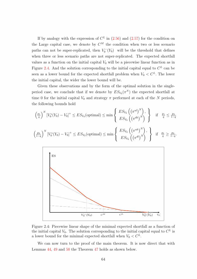
If by analogy with the expression of CL in (2.56) and (2.57) for the condition on
the Large capital case, we denote by CM the condition when two or less scenario
paths can not be super-replicated, then V −0 (Y0) will be the threshold that defines
when three or less scenario paths are not super-replicated. The expected shortfall
values as a function on the initial capital V0 will be a piecewise linear function as in
Figure 2.4. And the solution corresponding to the initial capital equal to CL can be
seen as a lower bound for the expected shortfall problem when V0 < CL. The lower
the initial capital, the wider the lower bound will be.
Given these observations and by the form of the optimal solution in the single-
period case, we conclude that if we denote by ESV0(πN) the expected shortfall at
time 0 for the initial capital V0 and strategy π performed at each of the N periods,
the following bounds hold(p1
q
)N
[V ∗0 (Y0)− V0]
+ ≤ ESV0(optimal) ≤ min
ESV0
((πul)N)
,
ESV0
((πdh)N)
if p1
q≤ p3
1−q
(p3
1−q
)N
[V ∗0 (Y0)− V0]
+ ≤ ESV0(optimal) ≤ min
ESV0
((πuh)N)
,
ESV0
((πdl)N)
if p1
q≥ p3
1−q.
Figure 2.4: Piecewise linear shape of the minimal expected shortfall as a function ofthe initial capital V0. The solution corresponding to the initial capital equal to CL isa lower bound for the minimal expected shortfall when V0 < CL.
We can now turn to the proof of the main theorem. It is now direct that with
Lemmas 44, 49 and 50 the Theorem 47 holds as shown below.
64
Proof of Theorem 47. For n = N−1, and by the Dynamic Programming Principle
(see [6]),
J (L)(N − 1, SN−1, YN−1, VN−1) = infπ
E[(H(YN)− VN)+|SN−1, YN−1, VN−1
]. (2.58)
The goal at the stepN−1 is to find the minimum and the minimiser π in (2.58). Under
the assumption (1− q)V ∗N(YN−1h) + qV ∗
N(YN−1l) ≤ VN−1, we can use Lemma 44 and
Section 2.3.6.1 to show that equations (2.51) and (2.52) hold for n = N − 1. We now
proceed by induction with respect to n. Assume p1
q≤ p3
1−qand that Equation (2.51)
is valid at n+ 1 this is J(n+ 1, Sn+1, Yn+1, Vn+1) =(
p1
q∗1
)N−n−1 [V ∗
n+1(Yn+1)− Vn+1
]+then
E [J(n+ 1, Sn+1, Yn+1, Vn+1)|Sn, Yn, Vn] =
=
(p1
q∗1
)N−n−1
E
[[V ∗
n+1(Ynηn+1)− Vn − (ξn+1 − 1)
V ∗
n+1(Ynh)− Vn
(d− 1)
]+]
=
(p1
q∗1
)N−n−1p1
q
[V ∗
n+1(Yn h)− Vn
]++p2
q
[(1− q)V ∗
n+1(Ynh) + qV ∗n+1(Ynl)− Vn
]+and assuming (1− q)V ∗
n+2(Yn+1h) + qV ∗n+2(Yn+1l)− Vn+1 ≤ 0 it remains,
=
(p1
q
)N−n [V ∗
n+1(Yn h)− Vn
]+=
(p1
q
)N−n
[V ∗n (Yn)− Vn]+ = J(n, Sn, Yn, Vn).
Finally, Equation (2.53) follows from Lemma 49. The validity of (1−q)V ∗n+1(Ynh)+
qV ∗n+1(Ynl) ≤ Vn for all n = 0, ..., N − 1 follows from Lemma 50.
The case p1
q≥ p3
1−qcan be proved similarly.
2.3.6.4 The large capital case and the two-step procedure
We are now in a position to check whether the solution to the minimal expected
shortfall for the large initial capital case in Theorem 47 is the same as the given by
the two-step procedure in Proposition 42.
For STEP 1 in Proposition 42, we need to characterise the modified claim that
solves the minimal expected shortfall problem. We use the intuition given in Section
2.3.6.1 summarised as follows:
1. The optimal portfolio minimises the expected shortfall.
2. The Radon-Nikodym derivative dPdQ∗ acts as a selection procedure to the “worst-
case scenario” path ω.
65
3. The optimal portfolio super-replicates the contingent claim except in the “worst-
case scenario” path ω,
V V0,πN (ω) < HN(ω) and V V0,π
N (ω) ≥ HN(ω) in ω ∈ Ω\ω.
4. The shortfall is non-zero at the “worst-case scenario” path ω and zero
otherwise.
These facts suggests a representation of the final value of the optimal portfolio as
VN(ω) := HN(ω)1 dPdQ∗ (ω)>η∗ + γ1 dP
dQ∗ (ω)=η∗
with η∗ := minω∈Ω
dP
dQ∗ (ω)
, and γ such that matches the shortfall value. We can
formulate the modified claim as a corollary to Theorem 47.
Corollary 51 Define the modified claim VN(ω) as
VN(ω) := HT (ω)1 dPdQ∗ (ω)>η∗ + γ1 dP
dQ∗ (ω)=η∗
with
γ =V0 − E∗
[HN1 dP
dQ∗ (ω)>η∗]
E∗[1 dP
dQ∗ (ω)=η∗] .
If V V0,πN represents the optimal portfolio strategy to the Large initial capital case
in Theorem 47, then we have
V V0,πN = VN P-a.s.
Proof. Assume ω represents the worst-case scenario path of Section 2.3.6.1. It
is direct to see that ω = ω =
dPdQ∗ (ω) = η∗
, P-a.s. Then the representation
VN(ω) := HN(ω)1 dPdQ∗ (ω)>η∗ + γ1 dP
dQ∗ (ω)=η∗ is clear. It remains to show that γ
selected in this way is the right choice. On the scenario path ω
HT (ω)− VT (ω) = HT (ω)− γ =
(
1q∗1
)N
[V ∗0 (Y0)− V0]1ω0,0,N
0if p1
q∗1≤ p3
q∗3(1q∗3
)N
[V ∗0 (Y0)− V0]1ω0,0,N
0if p1
q∗1≥ p3
q∗3
66
or equivalently,
γ = HT (ω)− 1
Q∗ [ω][V ∗
0 (Y0)− V0]
=V0 + Q∗ [ω]HT (ω)− E∗ [HN ]
Q∗ [ω]
=V0 − (1−Q∗ [ω])E∗ [HN1ω 6=ω ]
Q∗ [ω]
=V0 − E∗
[HN1 dP
dQ∗ (ω)>η∗]
E∗[1 dP
dQ∗ (ω)=η∗] .
In order to fully prove STEP 1 in Proposition 42 about the modified claim that
solves the minimal expected shortfall problem we need to show that it indeed satisfies
the conditions in Proposition 42. Furthermore, if STEP 2 also holds, then the solution
to the N -period Large initial capital case in Theorem 47 is indeed equivalent to
that obtained by the two-step algorithm (dual formulation to the minimal expected
shortfall problem). These is guaranteed in the next proposition.
Proposition 52 The solution to the N-period Large capital case in Theorem 47 is
equivalent to the one given by the two-step procedure in Proposition 42. Furthermore,
as the two-step procedure reflects the dual formulation to the problem (see Appendix
B), in the present setting the dual pair is given by
(η, Q) :=
(minω∈Ω
dPdQ∗ (ω)
,Q∗
)Proof. The proof follows immediately from Theorem 47 and the representation of
the modified claim in Corollary 51. The inequalities VN ≤ HN and E∗[VN
]≤ V0
are a direct consequence of the representation of the modified claim. Then VN ∈V∞. By Theorem 47, the fact that VN minimises the expected shortfall implies that
VN = arg minV ∈VbE [HT − VT ] . This proves that VN satisfies STEP1 in Proposition
42. For STEP 2, VN is a super-replicating strategy also by Theorem 47. Finally, the
specification of the Dual pair is a consequence to the representation of the modified
claim.
2.3.6.5 Numerical example
Example 53 Consider the following example for N = 2, and
S0 = 50 u = 2 d = 0.25 p1 = 1/6 p2 = 5/16Y0 = 100 h = 1.5 l = 1 p3 = 1/2 p4 = 1/48
67
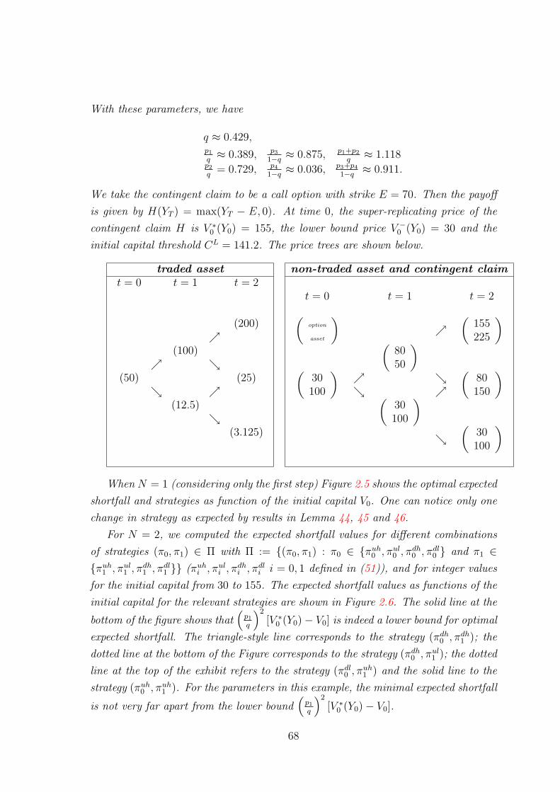
With these parameters, we have
q ≈ 0.429,p1
q≈ 0.389, p3
1−q≈ 0.875, p1+p2
q≈ 1.118
p2
q= 0.729, p4
1−q≈ 0.036, p3+p4
1−q≈ 0.911.
We take the contingent claim to be a call option with strike E = 70. Then the payoff
is given by H(YT ) = max(YT − E, 0). At time 0, the super-replicating price of the
contingent claim H is V ∗0 (Y0) = 155, the lower bound price V −
0 (Y0) = 30 and the
initial capital threshold CL = 141.2. The price trees are shown below.
traded asset non-traded asset and contingent claimt = 0 t = 1 t = 2
(200)
(100)
(50) (25)
(12.5)
(3.125)
t = 0 t = 1 t = 2(option
asset
)
(155225
)(
8050
)(
30100
)
(80150
)(
30100
)
(30100
)
When N = 1 (considering only the first step) Figure 2.5 shows the optimal expected
shortfall and strategies as function of the initial capital V0. One can notice only one
change in strategy as expected by results in Lemma 44, 45 and 46.
For N = 2, we computed the expected shortfall values for different combinations
of strategies (π0, π1) ∈ Π with Π := (π0, π1) : π0 ∈ πuh0 , πul
0 , πdh0 , π
dl0 and π1 ∈
πuh1 , πul
1 , πdh1 , π
dl1 (πuh
i , πuli , π
dhi , π
dli i = 0, 1 defined in (51)), and for integer values
for the initial capital from 30 to 155. The expected shortfall values as functions of the
initial capital for the relevant strategies are shown in Figure 2.6. The solid line at the
bottom of the figure shows that(
p1
q
)2
[V ∗0 (Y0)− V0] is indeed a lower bound for optimal
expected shortfall. The triangle-style line corresponds to the strategy (πdh0 , π
dh1 ); the
dotted line at the bottom of the Figure corresponds to the strategy (πdh0 , π
ul1 ); the dotted
line at the top of the exhibit refers to the strategy (πdl0 , π
uh1 ) and the solid line to the
strategy (πuh0 , πuh
1 ). For the parameters in this example, the minimal expected shortfall
is not very far apart from the lower bound(
p1
q
)2
[V ∗0 (Y0)− V0].
68
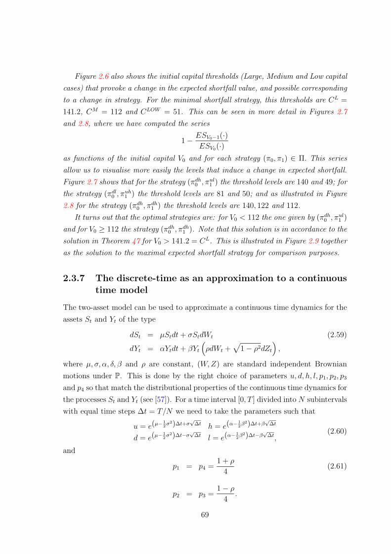
Figure 2.6 also shows the initial capital thresholds (Large, Medium and Low capital
cases) that provoke a change in the expected shortfall value, and possible corresponding
to a change in strategy. For the minimal shortfall strategy, this thresholds are CL =
141.2, CM = 112 and CLOW = 51. This can be seen in more detail in Figures 2.7
and 2.8, where we have computed the series
1− ESV0−1(·)ESV0(·)
as functions of the initial capital V0 and for each strategy (π0, π1) ∈ Π. This series
allow us to visualise more easily the levels that induce a change in expected shortfall.
Figure 2.7 shows that for the strategy (πdh0 , π
ul1 ) the threshold levels are 140 and 49; for
the strategy (πdl0 , π
uh1 ) the threshold levels are 81 and 50; and as illustrated in Figure
2.8 for the strategy (πdh0 , π
dh1 ) the threshold levels are 140, 122 and 112.
It turns out that the optimal strategies are: for V0 < 112 the one given by (πdh0 , π
ul1 )
and for V0 ≥ 112 the strategy (πdh0 , π
dh1 ). Note that this solution is in accordance to the
solution in Theorem 47 for V0 > 141.2 = CL. This is illustrated in Figure 2.9 together
as the solution to the maximal expected shortfall strategy for comparison purposes.
2.3.7 The discrete-time as an approximation to a continuoustime model
The two-asset model can be used to approximate a continuous time dynamics for the
assets St and Yt of the type
dSt = µStdt+ σStdWt (2.59)
dYt = αYtdt+ βYt
(ρdWt +
√1− ρ2dZt
),
where µ, σ, α, δ, β and ρ are constant, (W,Z) are standard independent Brownian
motions under P. This is done by the right choice of parameters u, d, h, l, p1, p2, p3
and p4 so that match the distributional properties of the continuous time dynamics for
the processes St and Yt (see [57]). For a time interval [0, T ] divided into N subintervals
with equal time steps ∆t = T/N we need to take the parameters such that
u = e(µ− 12σ2)∆t+σ
√∆t h = e(α− 1
2β2)∆t+β
√∆t
d = e(µ− 12σ2)∆t−σ
√∆t l = e(α− 1
2β2)∆t−β
√∆t,
(2.60)
and
p1 = p4 =1 + ρ
4(2.61)
p2 = p3 =1− ρ
4.
69
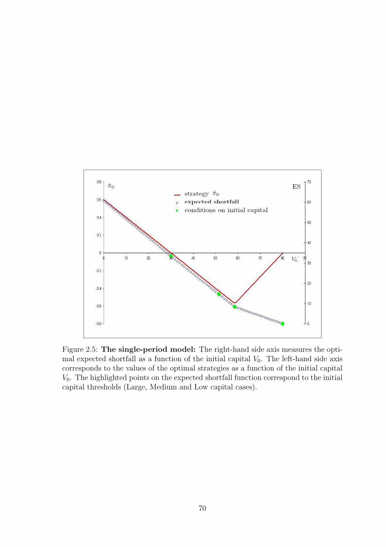
Figure 2.5: The single-period model: The right-hand side axis measures the opti-mal expected shortfall as a function of the initial capital V0. The left-hand side axiscorresponds to the values of the optimal strategies as a function of the initial capitalV0. The highlighted points on the expected shortfall function correspond to the initialcapital thresholds (Large, Medium and Low capital cases).
70
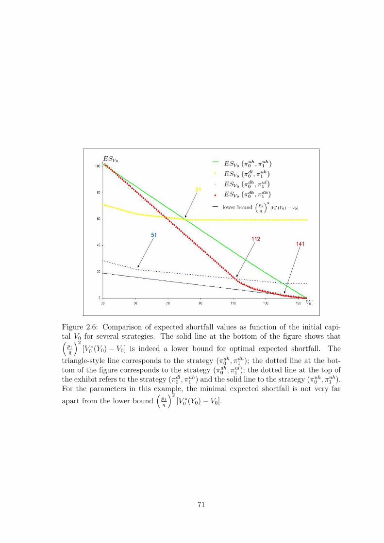
Figure 2.6: Comparison of expected shortfall values as function of the initial capi-tal V0 for several strategies. The solid line at the bottom of the figure shows that(
p1
q
)2
[V ∗0 (Y0)− V0] is indeed a lower bound for optimal expected shortfall. The
triangle-style line corresponds to the strategy (πdh0 , π
dh1 ); the dotted line at the bot-
tom of the figure corresponds to the strategy (πdh0 , π
ul1 ); the dotted line at the top of
the exhibit refers to the strategy (πdl0 , π
uh1 ) and the solid line to the strategy (πuh
0 , πuh1 ).
For the parameters in this example, the minimal expected shortfall is not very far
apart from the lower bound(
p1
q
)2
[V ∗0 (Y0)− V0].
71
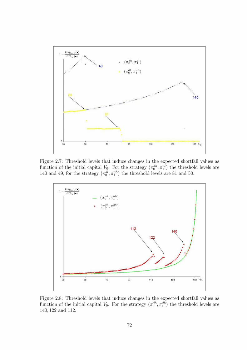
Figure 2.7: Threshold levels that induce changes in the expected shortfall values asfunction of the initial capital V0. For the strategy (πdh
0 , πul1 ) the threshold levels are
140 and 49; for the strategy (πdl0 , π
uh1 ) the threshold levels are 81 and 50.
Figure 2.8: Threshold levels that induce changes in the expected shortfall values asfunction of the initial capital V0. For the strategy (πdh
0 , πdh1 ) the threshold levels are
140, 122 and 112.
72
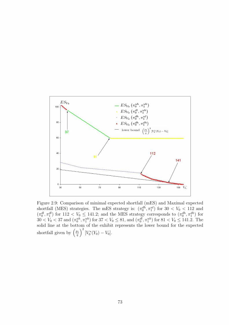
Figure 2.9: Comparison of minimal expected shortfall (mES) and Maximal expectedshortfall (MES) strategies. The mES strategy is: (πdh
0 , πul1 ) for 30 < V0 < 112 and
(πdl0 , π
dl1 ) for 112 < V0 ≤ 141.2; and the MES strategy corresponds to (πdh
0 , πdh1 ) for
30 < V0 < 37 and (πuh0 , πuh
1 ) for 37 < V0 ≤ 81, and (πdl0 , π
uh1 ) for 81 < V0 ≤ 141.2. The
solid line at the bottom of the exhibit represents the lower bound for the expected
shortfall given by(
p1
q
)2
[V ∗0 (Y0)− V0].
73
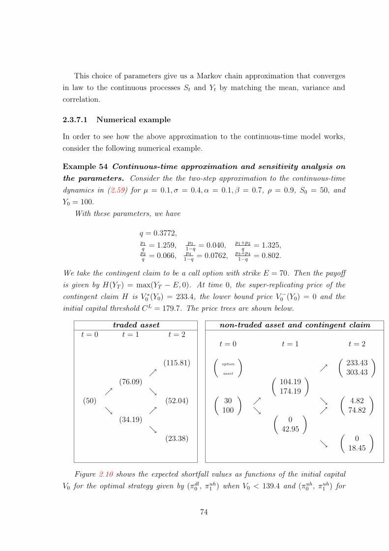
This choice of parameters give us a Markov chain approximation that converges
in law to the continuous processes St and Yt by matching the mean, variance and
correlation.
2.3.7.1 Numerical example
In order to see how the above approximation to the continuous-time model works,
consider the following numerical example.
Example 54 Continuous-time approximation and sensitivity analysis on
the parameters. Consider the the two-step approximation to the continuous-time
dynamics in (2.59) for µ = 0.1, σ = 0.4, α = 0.1, β = 0.7, ρ = 0.9, S0 = 50, and
Y0 = 100.
With these parameters, we have
q = 0.3772,p1
q= 1.259, p3
1−q= 0.040, p1+p2
q= 1.325,
p2
q= 0.066, p4
1−q= 0.0762, p3+p4
1−q= 0.802.
We take the contingent claim to be a call option with strike E = 70. Then the payoff
is given by H(YT ) = max(YT − E, 0). At time 0, the super-replicating price of the
contingent claim H is V ∗0 (Y0) = 233.4, the lower bound price V −
0 (Y0) = 0 and the
initial capital threshold CL = 179.7. The price trees are shown below.
traded asset non-traded asset and contingent claimt = 0 t = 1 t = 2
(115.81)
(76.09)
(50) (52.04)
(34.19)
(23.38)
t = 0 t = 1 t = 2(option
asset
)
(233.43303.43
)(
104.19174.19
)(
30100
)
(4.8274.82
)(
042.95
)
(0
18.45
)
Figure 2.10 shows the expected shortfall values as functions of the initial capital
V0 for the optimal strategy given by (πdl0 , π
uh1 ) when V0 < 139.4 and (πuh
0 , πuh1 ) for
74
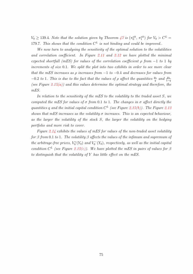
V0 ≥ 139.4. Note that the solution given by Theorem 47 is (πuh0 , πuh
1 ) for V0 > CL =
179.7. This shows that the condition CL is not binding and could be improved..
We now turn to analysing the sensitivity of the optimal solution to the volatilities
and correlation coefficient. In Figure 2.11 and 2.12 we have plotted the minimal
expected shortfall (mES) for values of the correlation coefficient ρ from −1 to 1 by
increments of size 0.1. We split the plot into two exhibits in order to see more clear
that the mES increases as ρ increases from −1 to −0.4 and decreases for values from
−0.2 to 1. This is due to the fact that the values of ρ affect the quantities p1
qand p3
1−q
(see Figure 2.15(a)) and this values determine the optimal strategy and therefore, the
mES.
In relation to the sensitivity of the mES to the volatility to the traded asset S, we
computed the mES for values of σ from 0.1 to 1. The changes in σ affect directly the
quantities q and the initial capital condition CL (see Figure 2.15(b)). The Figure 2.13
shows that mES increases as the volatility σ increases. This is an expected behaviour,
as the larger the volatility of the stock S, the larger the volatility on the hedging
portfolio and more risk to cover.
Figure 2.14 exhibits the values of mES for values of the non-traded asset volatility
for β from 0.1 to 1. The volatility β affects the values of the infimum and supremum of
the arbitrage-free prices, V ∗0 (Y0) and V −
0 (Y0), respectively, as well as the initial capital
condition CL (see Figure 2.15(c)). We have plotted the mES in pairs of values for β
to distinguish that the volatility of Y has little effect on the mES.
75
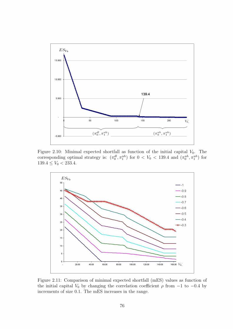
Figure 2.10: Minimal expected shortfall as function of the initial capital V0. Thecorresponding optimal strategy is: (πdl
0 , πuh1 ) for 0 < V0 < 139.4 and (πuh
0 , πuh1 ) for
139.4 ≤ V0 < 233.4.
Figure 2.11: Comparison of minimal expected shortfall (mES) values as function ofthe initial capital V0 by changing the correlation coefficient ρ from −1 to −0.4 byincrements of size 0.1. The mES increases in the range.
76
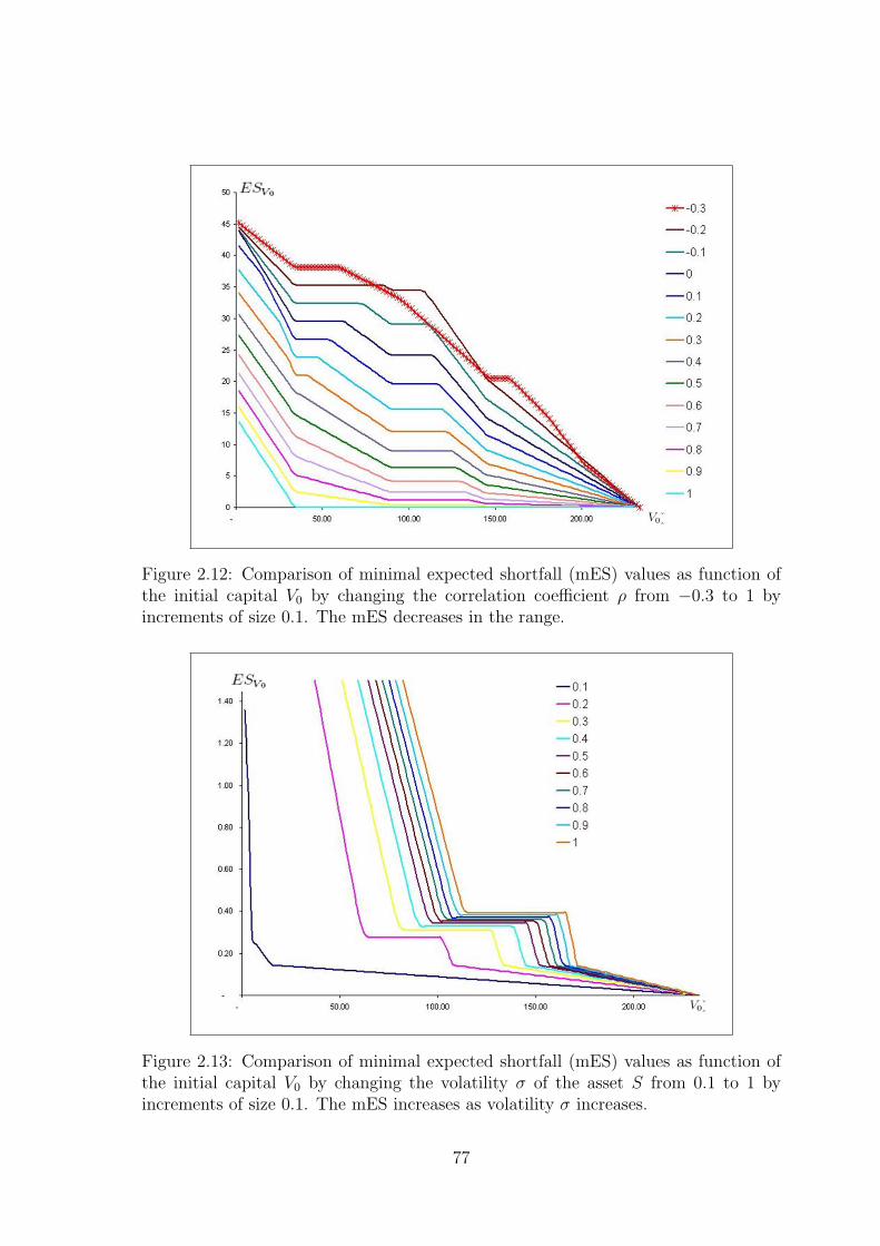
Figure 2.12: Comparison of minimal expected shortfall (mES) values as function ofthe initial capital V0 by changing the correlation coefficient ρ from −0.3 to 1 byincrements of size 0.1. The mES decreases in the range.
Figure 2.13: Comparison of minimal expected shortfall (mES) values as function ofthe initial capital V0 by changing the volatility σ of the asset S from 0.1 to 1 byincrements of size 0.1. The mES increases as volatility σ increases.
77
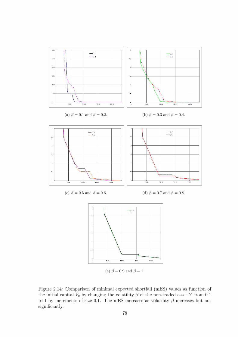
(a) β = 0.1 and β = 0.2. (b) β = 0.3 and β = 0.4.
(c) β = 0.5 and β = 0.6. (d) β = 0.7 and β = 0.8.
(e) β = 0.9 and β = 1.
Figure 2.14: Comparison of minimal expected shortfall (mES) values as function ofthe initial capital V0 by changing the volatility β of the non-traded asset Y from 0.1to 1 by increments of size 0.1. The mES increases as volatility β increases but notsignificantly.
78
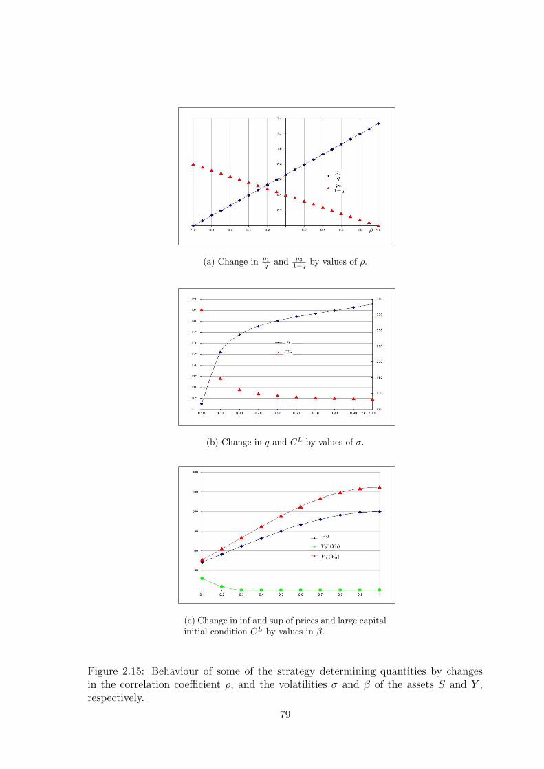
(a) Change in p1q and p3
1−q by values of ρ.
(b) Change in q and CL by values of σ.
(c) Change in inf and sup of prices and large capitalinitial condition CL by values in β.
Figure 2.15: Behaviour of some of the strategy determining quantities by changesin the correlation coefficient ρ, and the volatilities σ and β of the assets S and Y ,respectively.
79
Part II
Risk and Hedging inContinuous-time: Ito Diffusion
Models
80
Chapter 3
WCS, VaR and AVaR
3.1 Introduction
Assume we work under a complete probability space (Ω,F ,P), where the probability
P is assumed to be the “real” or “physical” probability measure (data generating),
which is objective and assumed unique. Let also assume our space supports a random
variable (or process) X that represents a risky asset for which we need to compute
risk. When X is model-dependent, this is, when the probability P on Ω is explicitly
given, we can in many cases compute WCS, VaR, and AVaR. A special case of model-
dependence is when X is given by a Markov diffusion process, and as they are the
most common models used in finance, we devote this chapter to the study of the
computation of our three measures of risk (WCS, VaR, and AVaR) for positions
driven by one-dimensional continuous Markov diffusion processes.
Note that although we carry our analysis only for WCS, VaR, and AVaR, most of
our procedures can also be applied to other similar measures of risk.
The main idea to compute risk given by VaR or AVaR of a position X modelled
as a continuous diffusion process is to exploit its Markov property and characterise it
as the solution to a second order partial differential equation (PDE) with boundary
conditions. In the case of the WCS risk measure, the approach is similar but less
direct as WCS is defined as the supremum over a set of probability measures. In
order to obtain WCS also as the solution to a boundary value PDE we need to state
conditions on the set of measures, so the supremum in the definition of WCS is finite.
Motivated by practical applications, firstly, we analyse in detail the case when un-
der each measure on the definition of WCS the process X remains a Markov diffusion
process. This involves the study of properties of what are called exponential change
of measure transformations of Markov processes.
81
In most of the cases, the PDEs that characterise the risk measures do not have
explicit solutions and series expansions or numerical methods need to be applied. In
the few cases that do allow explicit solutions, solving for the risk PDEs and solving
for the transition probability density of the process X are equivalent. This is shown
in the last part of the chapter.
When the restriction on the Markov property is lifted, we establish conditions so
the computation of WCS can be formulated as a stochastic control problem and then
as the solution to a nonlinear PDE of second order with boundary conditions. We
complement the chapter with several examples.
3.2 The model
For simplicity in the notation, we assume through this chapter that our time horizon
is [t0, T ], with 0 ≤ t0 ≤ T , unless otherwise stated.
Let the process Xt ∈ R be such that its dynamics are given by the following
one-dimensional SDE
dXt = b(Xt)dt + a(Xt)dWt, Xt0 = x0 (Xt-SDE)
with a, b given deterministic functions satisfying b : R → R, a : R → (0,∞), and Wt a
one-dimensional Brownian motion. We need the following assumption on the process
X.
Assumption 55 We assume that the functions a and b have sufficient regularity
properties to ensure that the stochastic differential equation in (Xt-SDE) for the pro-
cess Xt has a path-wise unique solution, non-explosive strong solution (cf [51, Section
5.3 p. 300] or [77, Chapter 5]), and Ftt0≤t≤T is its natural filtration.
Assumption 56 We assume the process Xt has a transition probability density p(x, t; τ, y).
This is the case for some conditions on the functions a, and b (see [51] p. 369, [92,
p. 500] or [86, Theo 3.2.1, Cor. 3.22 and Theo 3.2.6 p. 71-77]). Furthermore, we
also assume the conditions needed by the Feynman-Kac representation theorem hold
(see [51, Theo 7.6 p. 366] or [92, Theo 3.33 p. 497]) so p(x, t; τ, y) allows a unique
stochastic representations.
The homogeneous infinitesimal generator associated with the SDE in (Xt-SDE) is
given by
Gb,a[f ](x) :=1
2a2(x)
∂2f
∂x2+ b(x)
∂f
∂x.
82
The main idea for computing WCSP , VaRα and AVaRα for processes Xt as in
(Xt-SDE) is to exploit their Markov property and formulate the risk measures as the
solution of a PDE.
3.3 Worst Conditional Scenario risk measure (WCS)
By the definition of WCSP in Chapter 1, recalled below
WCSP(X) = supQ∈P
EQ [−X]
we fix a priori a subset P (called set of priors) of the set of all probability measures on
(Ω,F). It is necessary that each measure Q ∈P respects P-null sets, for otherwise a
stochastic integral defined with respect to P might make no sense under Q. Therefore
we make the following assumption.
Assumption 57 The set of reference measures P used in WCSP is a subset of
Ma(P).
Note that WCSP is “well defined” if the set P is such that supQ∈P EQ [−X] <∞.
In particular, this is satisfied if X ∈ L∞(Ω,F ,P) on [t0, T ], P is convex, and the set
DP :=
dQdP : Q ∈P
is weakly compact in L1(Ω,F ,P). In other words, for a bounded
position X, and Z ∈ DP we have
J−X(Z) = E [−XZ] = EQ [−X] <∞.
J−X(Z) is a linear functional and by the assumption that the set DP is weakly com-
pact, the above relation also holds for the infimum and supremum of the elements in
the set DP . This is,
supZ∈DP
J−X(Z) = supQ∈P
EQ [−X] <∞
and
infZ∈DP
J−X(Z) = infQ∈P
EQ [−X] <∞.
On the other hand, if there exist sets A ⊂ Ω for which Q [A] = 0 for all Q ∈P and
P [A] 6= 0 they may cause problems in the definition of WCS. Therefore, we assume,
as follows:
Assumption 58 We assume P ⊂Ma(P) is convex, the set DP :=
dQdP : Q ∈P
is
weakly compact in L1(Ω,F ,P) and P [A] = 0 if and only if Q [A] = 0 for all Q ∈P.
In the case our risk horizon is [t0, t], so for computing WCSP on the position
X t−t0 = Xt−Xt0 , we need to know the dynamics of the process X under each of the
elements in P .
83
3.3.1 Change of measure
Change of measures are characterised by Girsanov theorem, which says (see [51, Sec.
3.5] or [77, Sec. 27]) that if Q is an absolutely continuous probability measure with
respect to P, then there exist an adapted processes ϕtt0≤t≤T with∫ T
t0ϕ2
sds < ∞(called Girsanov kernels) such that for
dQdP|Ft = Zt = Z(ϕ)t := exp
[∫ t
t0
ϕua(Xu)dWu −1
2
∫ t
t0
(ϕu)2a(Xu)
2du
]. (3.1)
Under the change of measure dQdP |Ft = Zt the process Xt under Q remains
dXt = γtdt + a(Xt)dWt (3.2)
with Xt0 = x0 ∈ R, and
γt = b(Xt) + a2(Xt)ϕt. (3.3)
And W is a Brownian motion under the measure Q
Remark 59 In the case Zt is a uniformly integrable P-martingale, the measure Q is
not only absolutely continuous with respect to P, but equivalent to P. A sufficient con-
dition for Zt to be uniformly integrable is the Novikov criterion E[exp
(12
∫ϕ2
sa2(Xs)ds
)]<
∞. See [51] for conditions on ϕt for Zt to be a uniformly integrable P-martingale.
Remark 60 It is a well known fact that an absolutely continuous change of measure
affects the process only in the drift term. From this observation, it is direct to see
that the WCSP risk measure can be interpreted as the risk due to uncertainty in the
drift. This is a special case of model risk.
One particular case of interest for computing WCS is when, under each measure in
the set P , the process Xt remains a Markov process. This includes the situation when
the process Xt is assumed to have a fixed functional structure (e.g. geometric Brow-
nian motion, Ornstein-Uhlenbeck processes, etc.) depending on some parameters.
But the “true” parameters are unknown, and instead, one considers some estimation
intervals on them. Computing WCS is then similar to considering the “worst-case
scenario” case of the expected value under the estimation intervals.
We analyse first the particular case when each of the measures Q ∈P defines a
Markov process, and then we explore some generalisations. If the set of measures Pis so that the Markov property is preserved on the process Xt under each Q ∈P, then
we can formulate the problem of computing WCS as a solution of a PDE. This will
be analysed in the next section.
84
3.3.2 Change of measure that preserves the Markov property
From the expression of the dynamics of Xt under the measure Q ∈P in (3.2) and
(3.3) we notice that for the process Xt to be Markov for Q ∈P, we need to impose
conditions on the Girsanov kernel ϕt in (3.1). The Markov property will be preserved
if ϕt only depends on the actual value of1 Xt, this is, ϕt needs to be of the form
ϕt = ψ(t,Xt), for some Ft-measurable function ψ : R+ × R → R+.
In terms of the density process Zt, any change of measure can also be expressed
(cf [47, Prop 3.8 p.155] or [51, Lemma 5.3 p.193]) as
EQ[X t−t0 ] =1
Z(ϕ)t0
E[X t−t0Z(ϕ)t].
Thus the dynamics of Xt under Q can be rewritten as,
dXt = γ(t,Xt)dt + a(Xt)dWt, (3.4)
for γ(t, x) = b(x) + a2(x)ψ(t, x).
Remark 61 Note that defining the density process Zt = Z(ψ(·, X·))t in (3.1) via
a time-dependent Girsanov kernel ψ(t,Xt) makes the process time-dependent as the
drift γ(t, x) = b(x) + a2(x)ψ(t, x) will depend on time.
This type of measure change that preserves the Markov property is called an
exponential change of measure for Markov processes (see [12], [65] and [8]).
3.3.2.1 Exponential change of measure for Markov processes
Before we motivate the exponential change of measure, we need to introduce some
notation.
Define by E (y)· the Doleans exponential for a martingale process y· on [0,∞) by
E (y)t := exp
[yt −
1
2[y]t
].
One can also think of E (y)· as the process zt = E (y)t such that defines the unique
solution to the equation
dzt = ztdyt, z0 = 1.
The equation above shows that E (y)t represents a martingale that has exponential
form (see [77, Ch. IV Sec. 19 p. 29] on Doleans exponential to define exponential
martingales).
1In general, a Girsanov kernel ϕt may depend on the past, or the whole path of the process X.
85
From the previous section on changes of measure that preserve the Markov prop-
erty, the Radon-Nikodym derivative remains
dQdP|Ft = exp
[∫ t
0
ψ(u,Xu)a(Xu)dWu −1
2
∫ t
0
(ψ(u,Xu))2a(Xu)
2du
](3.5)
= E(∫ t
0
ψ(u,Xu)a(Xu)dWu
)= Zt
= Z(ψ(·, X·))t
= h(t,Xt)
with h : R+ × R → R+ a Ft-measurable function (the function h can be seen as the
composition of the function Z by ψ).
The right-hand side on the first and second equalities in the set of equations in
(3.5) are local-martingales by construction, which is a condition for a density process
to define a proper change of measure. This implies that the function h(t, x) cannot
be just any function. We require conditions on h such that the process h(t,Xt) is a
P-martingale.
In the rest of the section, we study conditions for the function h to define a
Markov change of measure and use it to formulate the problem of computing WCSP
of a position X t−t0 with dynamics for Xt in (Xt-SDE) as the solution of a PDE.
For f ∈ C1,2 define the time-dependent infinitesimal generator Lγ,a associated with
the dynamics of Xt in (3.4) by
Lγ,a[f ](t, x) ,∂f
∂t+
1
2a2(x)
∂2f
∂x2+ γ(t, x)
∂f
∂x
=∂f
∂t+ Gγ,a[f ](x).
Remark 62 We will indistinguishably denote the partial derivative with respect to
the second variable of a function f(t, x) by ∂f∂x
(t, x) or fx(t, x). Similarly for any
other partial derivative. We will also omit their explicit dependency on the variables
when no confusion arises.
For f ∈ C1,2 define the process
J (f)t := f(t,Xt)− f(t0, x0)−∫ t
t0
Lb,a[f ](s,Xs)ds. (3.6)
86
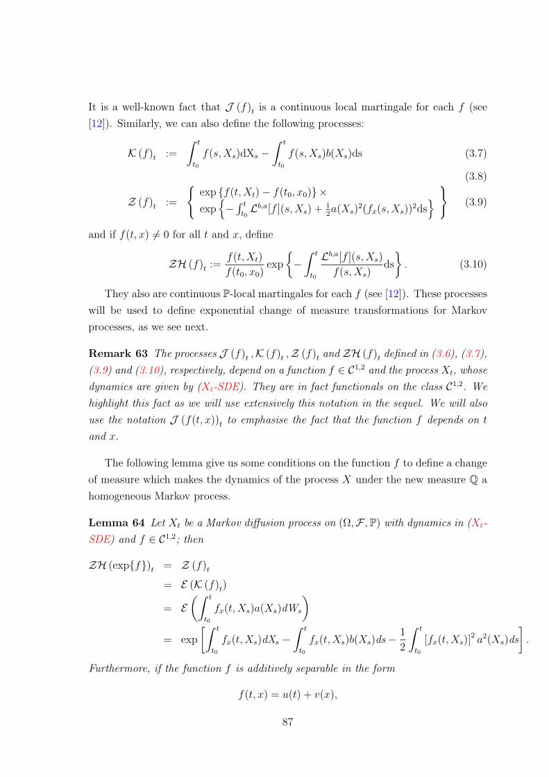
It is a well-known fact that J (f)t is a continuous local martingale for each f (see
[12]). Similarly, we can also define the following processes:
K (f)t :=
∫ t
t0
f(s,Xs)dXs −∫ t
t0
f(s,Xs)b(Xs)ds (3.7)
(3.8)
Z (f)t :=
exp f(t,Xt)− f(t0, x0)×exp
−∫ t
t0Lb,a[f ](s,Xs) + 1
2a(Xs)
2(fx(s,Xs))2ds
(3.9)
and if f(t, x) 6= 0 for all t and x, define
ZH (f)t :=f(t,Xt)
f(t0, x0)exp
−∫ t
t0
Lb,a[f ](s,Xs)
f(s,Xs)ds
. (3.10)
They also are continuous P-local martingales for each f (see [12]). These processes
will be used to define exponential change of measure transformations for Markov
processes, as we see next.
Remark 63 The processes J (f)t ,K (f)t ,Z (f)t and ZH (f)t defined in (3.6), (3.7),
(3.9) and (3.10), respectively, depend on a function f ∈ C1,2 and the process Xt, whose
dynamics are given by (Xt-SDE). They are in fact functionals on the class C1,2. We
highlight this fact as we will use extensively this notation in the sequel. We will also
use the notation J (f(t, x))t to emphasise the fact that the function f depends on t
and x.
The following lemma give us some conditions on the function f to define a change
of measure which makes the dynamics of the process X under the new measure Q a
homogeneous Markov process.
Lemma 64 Let Xt be a Markov diffusion process on (Ω,F ,P) with dynamics in (Xt-
SDE) and f ∈ C1,2; then
ZH (expf)t = Z (f)t
= E (K (f)t)
= E(∫ t
t0
fx(t,Xs)a(Xs)dWs
)= exp
[∫ t
t0
fx(t,Xs)dXs −∫ t
t0
fx(t,Xs)b(Xs)ds−1
2
∫ t
t0
[fx(t,Xs)]2 a2(Xs)ds
].
Furthermore, if the function f is additively separable in the form
f(t, x) = u(t) + v(x),
87
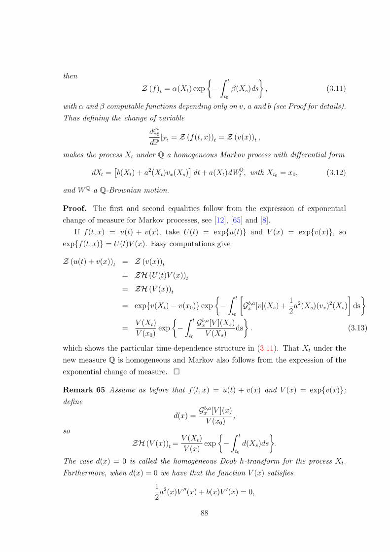
then
Z (f)t = α(Xt) exp
−∫ t
t0
β(Xs)ds
, (3.11)
with α and β computable functions depending only on v, a and b (see Proof for details).
Thus defining the change of variable
dQdP|Ft = Z (f(t, x))t = Z (v(x))t ,
makes the process Xt under Q a homogeneous Markov process with differential form
dXt =[b(Xt) + a2(Xt)vx(Xs)
]dt + a(Xt)dW
Qt , with Xt0 = x0, (3.12)
and WQ a Q-Brownian motion.
Proof. The first and second equalities follow from the expression of exponential
change of measure for Markov processes, see [12], [65] and [8].
If f(t, x) = u(t) + v(x), take U(t) = expu(t) and V (x) = expv(x), so
expf(t, x) = U(t)V (x). Easy computations give
Z (u(t) + v(x))t = Z (v(x))t
= ZH (U(t)V (x))t
= ZH (V (x))t
= expv(Xt)− v(x0) exp
−∫ t
t0
[Gb,a
x [v](Xs) +1
2a2(Xs)(vx)
2(Xs)
]ds
=
V (Xt)
V (x0)exp
−∫ t
t0
Gb,ax [V ](Xs)
V (Xs)ds
. (3.13)
which shows the particular time-dependence structure in (3.11). That Xt under the
new measure Q is homogeneous and Markov also follows from the expression of the
exponential change of measure.
Remark 65 Assume as before that f(t, x) = u(t) + v(x) and V (x) = expv(x);define
d(x) =Gb,a
x [V ](x)
V (x0),
so
ZH (V (x))t =V (Xt)
V (x)exp
−∫ t
t0
d(Xs)ds
.
The case d(x) = 0 is called the homogeneous Doob h-transform for the process Xt.
Furthermore, when d(x) = 0 we have that the function V (x) satisfies
1
2a2(x)V ′′(x) + b(x)V ′(x) = 0,
88
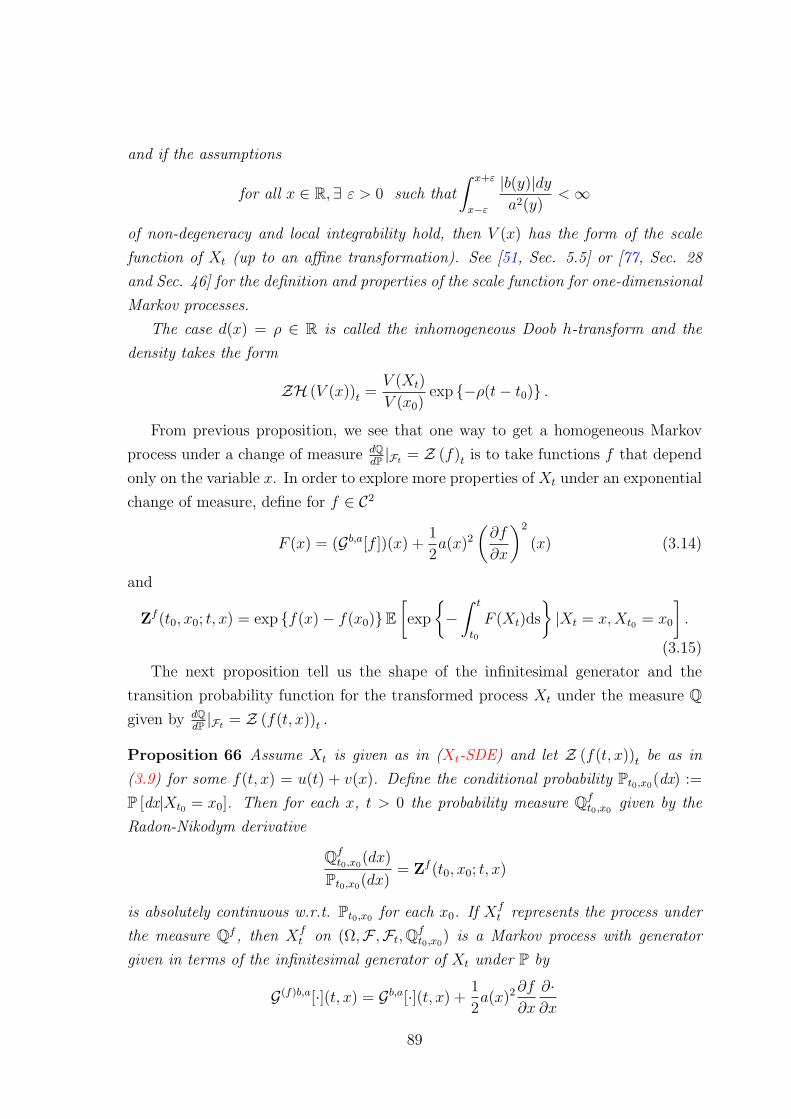
and if the assumptions
for all x ∈ R,∃ ε > 0 such that
∫ x+ε
x−ε
|b(y)|dya2(y)
<∞
of non-degeneracy and local integrability hold, then V (x) has the form of the scale
function of Xt (up to an affine transformation). See [51, Sec. 5.5] or [77, Sec. 28
and Sec. 46] for the definition and properties of the scale function for one-dimensional
Markov processes.
The case d(x) = ρ ∈ R is called the inhomogeneous Doob h-transform and the
density takes the form
ZH (V (x))t =V (Xt)
V (x0)exp −ρ(t− t0) .
From previous proposition, we see that one way to get a homogeneous Markov
process under a change of measure dQdP |Ft = Z (f)t is to take functions f that depend
only on the variable x. In order to explore more properties of Xt under an exponential
change of measure, define for f ∈ C2
F (x) = (Gb,a[f ])(x) +1
2a(x)2
(∂f
∂x
)2
(x) (3.14)
and
Zf (t0, x0; t, x) = exp f(x)− f(x0)E[exp
−∫ t
t0
F (Xt)ds
|Xt = x,Xt0 = x0
].
(3.15)
The next proposition tell us the shape of the infinitesimal generator and the
transition probability function for the transformed process Xt under the measure Qgiven by dQ
dP |Ft = Z (f(t, x))t .
Proposition 66 Assume Xt is given as in (Xt-SDE) and let Z (f(t, x))t be as in
(3.9) for some f(t, x) = u(t) + v(x). Define the conditional probability Pt0,x0(dx) :=
P [dx|Xt0 = x0]. Then for each x, t > 0 the probability measure Qft0,x0
given by the
Radon-Nikodym derivative
Qft0,x0
(dx)
Pt0,x0(dx)= Zf (t0, x0; t, x)
is absolutely continuous w.r.t. Pt0,x0 for each x0. If Xft represents the process under
the measure Qf , then Xft on (Ω,F ,Ft,Qf
t0,x0) is a Markov process with generator
given in terms of the infinitesimal generator of Xt under P by
G(f)b,a[·](t, x) = Gb,a[·](t, x) +1
2a(x)2∂f
∂x
∂·∂x
89
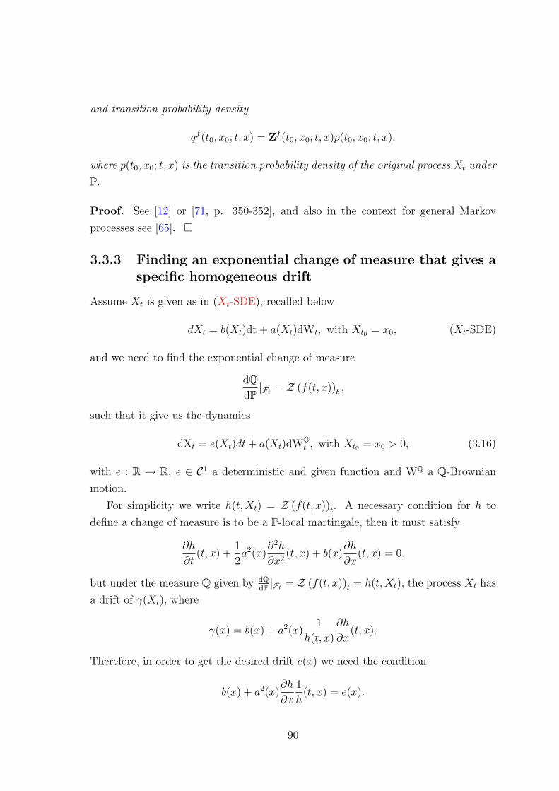
and transition probability density
qf (t0, x0; t, x) = Zf (t0, x0; t, x)p(t0, x0; t, x),
where p(t0, x0; t, x) is the transition probability density of the original process Xt under
P.
Proof. See [12] or [71, p. 350-352], and also in the context for general Markov
processes see [65].
3.3.3 Finding an exponential change of measure that gives aspecific homogeneous drift
Assume Xt is given as in (Xt-SDE), recalled below
dXt = b(Xt)dt + a(Xt)dWt, with Xt0 = x0, (Xt-SDE)
and we need to find the exponential change of measure
dQdP|Ft = Z (f(t, x))t ,
such that it give us the dynamics
dXt = e(Xt)dt+ a(Xt)dWQt , with Xt0 = x0 > 0, (3.16)
with e : R → R, e ∈ C1 a deterministic and given function and WQ a Q-Brownian
motion.
For simplicity we write h(t,Xt) = Z (f(t, x))t. A necessary condition for h to
define a change of measure is to be a P-local martingale, then it must satisfy
∂h
∂t(t, x) +
1
2a2(x)
∂2h
∂x2(t, x) + b(x)
∂h
∂x(t, x) = 0,
but under the measure Q given by dQdP |Ft = Z (f(t, x))t = h(t,Xt), the process Xt has
a drift of γ(Xt), where
γ(x) = b(x) + a2(x)1
h(t, x)
∂h
∂x(t, x).
Therefore, in order to get the desired drift e(x) we need the condition
b(x) + a2(x)∂h
∂x
1
h(t, x) = e(x).
90
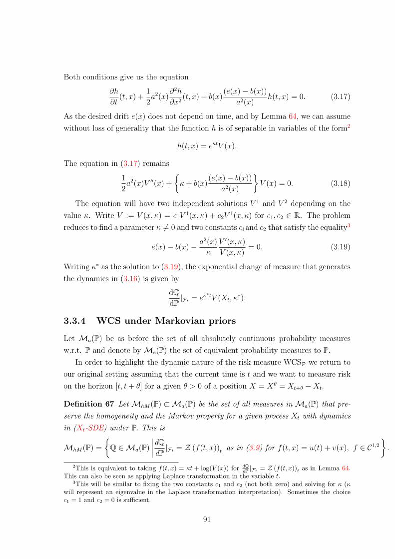
Both conditions give us the equation
∂h
∂t(t, x) +
1
2a2(x)
∂2h
∂x2(t, x) + b(x)
(e(x)− b(x))
a2(x)h(t, x) = 0. (3.17)
As the desired drift e(x) does not depend on time, and by Lemma 64, we can assume
without loss of generality that the function h is of separable in variables of the form2
h(t, x) = eκtV (x).
The equation in (3.17) remains
1
2a2(x)V ′′(x) +
κ+ b(x)
(e(x)− b(x))
a2(x)
V (x) = 0. (3.18)
The equation will have two independent solutions V 1 and V 2 depending on the
value κ. Write V := V (x, κ) = c1V1(x, κ) + c2V
1(x, κ) for c1, c2 ∈ R. The problem
reduces to find a parameter κ 6= 0 and two constants c1and c2 that satisfy the equality3
e(x)− b(x)− a2(x)
κ
V ′(x, κ)
V (x, κ)= 0. (3.19)
Writing κ∗ as the solution to (3.19), the exponential change of measure that generates
the dynamics in (3.16) is given by
dQdP|Ft = eκ∗tV (Xt, κ
∗).
3.3.4 WCS under Markovian priors
Let Ma(P) be as before the set of all absolutely continuous probability measures
w.r.t. P and denote by Me(P) the set of equivalent probability measures to P.
In order to highlight the dynamic nature of the risk measure WCSP we return to
our original setting assuming that the current time is t and we want to measure risk
on the horizon [t, t+ θ] for a given θ > 0 of a position X = Xθ = Xt+θ −Xt.
Definition 67 Let MhM(P) ⊂Ma(P) be the set of all measures in Ma(P) that pre-
serve the homogeneity and the Markov property for a given process Xt with dynamics
in (Xt-SDE) under P. This is
MhM(P) =
Q ∈Ma(P)
∣∣∣∣dQdP|Ft = Z (f(t, x))t as in (3.9) for f(t, x) = u(t) + v(x), f ∈ C1,2
.
2This is equivalent to taking f(t, x) = κt + log(V (x)) for dQdP |Ft
= Z (f(t, x))t as in Lemma 64.This can also be seen as applying Laplace transformation in the variable t.
3This will be similar to fixing the two constants c1 and c2 (not both zero) and solving for κ (κwill represent an eigenvalue in the Laplace transformation interpretation). Sometimes the choicec1 = 1 and c2 = 0 is sufficient.
91
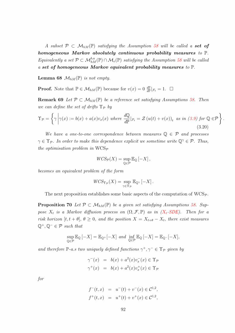
A subset P ⊂ MhM(P) satisfying the Assumption 58 will be called a set of
homogeneous Markov absolutely continuous probability measures to P.
Equivalently a set P ⊂Mb,ahM(P)∩Me(P) satisfying the Assumption 58 will be called
a set of homogeneous Markov equivalent probability measures to P.
Lemma 68 MhM(P) is not empty.
Proof. Note that P ∈MhM(P) because for v(x) = 0 dPdP |Ft = 1.
Remark 69 Let P ⊂ MhM(P) be a reference set satisfying Assumptions 58. Then
we can define the set of drifts ΥP by
ΥP =
γ
∣∣∣∣γ(x) := b(x) + a(x)vx(x) wheredQdP|Ft = Z (u(t) + v(x))t as in (3.9) for Q ∈P
.
(3.20)
We have a one-to-one correspondence between measures Q ∈ P and processes
γ ∈ ΥP . In order to make this dependence explicit we sometime write Qγ ∈ P. Thus,
the optimisation problem in WCSP
WCSP(X) = supQ∈P
EQ [−X] ,
becomes an equivalent problem of the form
WCSΥP (X) = supγ∈ΥP
EQγ [−X] .
The next proposition establishes some basic aspects of the computation of WCSP .
Proposition 70 Let P ⊂ MhM(P) be a given set satisfying Assumptions 58. Sup-
pose Xt is a Markov diffusion process on (Ω,F ,P) as in (Xt-SDE). Then for a
risk horizon [t, t + θ], θ ≥ 0, and the position X = Xt+θ − Xt, there exist measures
Q+,Q− ∈ P such that
supQ∈P
EQ [−X] = EQ+ [−X] and infQ∈P
EQ [−X] = EQ− [−X],
and therefore P-a.s two uniquely defined functions γ+, γ− ∈ ΥP given by
γ−(x) = b(x) + a2(x)v−x (x) ∈ ΥP
γ+(x) = b(x) + a2(x)v+x (x) ∈ ΥP
for
f−(t, x) = u−(t) + v−(x) ∈ C1,2,
f+(t, x) = u+(t) + v+(x) ∈ C1,2,
92
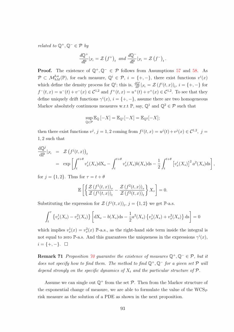
related to Q+,Q− ∈ P by
dQ+
dP|Ft = Z
(f+)
tand
dQ−
dP|Ft = Z
(f−)
t.
Proof. The existence of Q+,Q− ∈ P follows from Assumptions 57 and 58. As
P ⊂ Mb,ahM(P), for each measure, Qi ∈ P, i = +,−, there exist functions vi(x)
which define the density process for Qi; this is, dQi
dP |Ft = Z (f i(t, x))t, i = +,− for
f−(t, x) = u−(t) + v−(x) ∈ C1,2 and f+(t, x) = u+(t) + v+(x) ∈ C1,2. To see that they
define uniquely drift functions γi(x), i = +,−, assume there are two homogeneous
Markov absolutely continuous measures w.r.t P, say, Q1 and Q2 ∈ P such that
supQ∈P
EQ [−X] = EQ1 [−X] = EQ2 [−X];
then there exist functions vj, j = 1, 2 coming from f j(t, x) = uj(t)+vj(x) ∈ C1,2, j =
1, 2 such that
dQj
dP|Ft = Z
(f j(t, x)
)t
= exp
[∫ t+θ
t
vix(Xs)dXs −
∫ t+θ
t
vix(Xs)b(Xs)ds− 1
2
∫ t+θ
t
[vi
x(Xs)]2a2(Xs)ds
],
for j = 1, 2. Thus for τ = t+ θ
E[Z (f 1(t, x))τ
Z (f 1(t, x))t
− Z (f 2(t, x))τ
Z (f 2(t, x))t
Xτ
]= 0.
Substituting the expression for Z (f j(t, x))t, j = 1, 2 we get P-a.s.∫ τ
t
v1
x(Xs)− v2x(Xs)
[dXs − b(Xs)ds− 1
2a2(Xs)
v1
x(Xs) + v2x(Xs)
ds
]= 0
which implies v1x(x) = v2
x(x) P-a.s., as the right-hand side term inside the integral is
not equal to zero P-a.s. And this guarantees the uniqueness in the expressions γi(x),
i = +,−.
Remark 71 Proposition 70 guarantee the existence of measures Q+,Q− ∈ P, but it
does not specify how to find them. The method to find Q+,Q− for a given set P will
depend strongly on the specific dynamics of Xt and the particular structure of P.
Assume we can single out Q+ from the set P . Then from the Markov structure of
the exponential change of measure, we are able to formulate the value of the WCSP
risk measure as the solution of a PDE as shown in the next proposition.
93
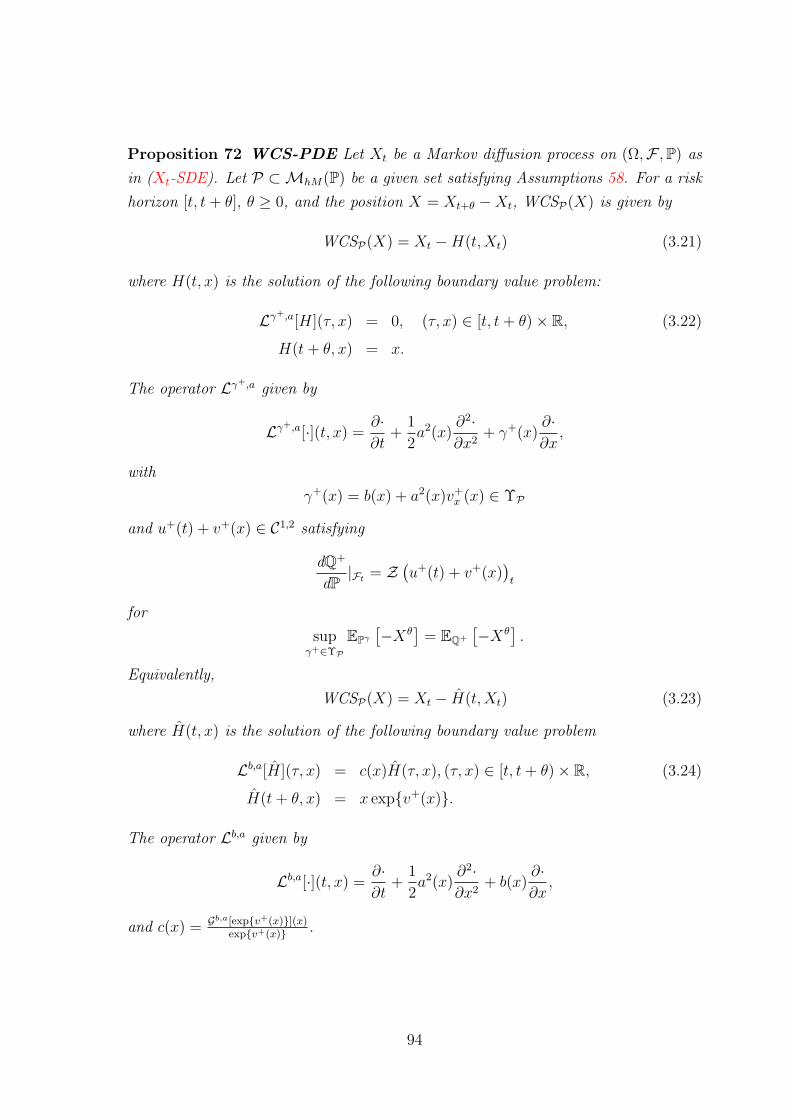
Proposition 72 WCS-PDE Let Xt be a Markov diffusion process on (Ω,F ,P) as
in (Xt-SDE). Let P ⊂MhM(P) be a given set satisfying Assumptions 58. For a risk
horizon [t, t+ θ], θ ≥ 0, and the position X = Xt+θ −Xt, WCSP(X) is given by
WCSP(X) = Xt −H(t,Xt) (3.21)
where H(t, x) is the solution of the following boundary value problem:
Lγ+,a[H](τ, x) = 0, (τ, x) ∈ [t, t+ θ)× R, (3.22)
H(t+ θ, x) = x.
The operator Lγ+,a given by
Lγ+,a[·](t, x) =∂·∂t
+1
2a2(x)
∂2·∂x2
+ γ+(x)∂·∂x,
with
γ+(x) = b(x) + a2(x)v+x (x) ∈ ΥP
and u+(t) + v+(x) ∈ C1,2 satisfying
dQ+
dP|Ft = Z
(u+(t) + v+(x)
)t
for
supγ+∈ΥP
EPγ
[−Xθ
]= EQ+
[−Xθ
].
Equivalently,
WCSP(X) = Xt − H(t,Xt) (3.23)
where H(t, x) is the solution of the following boundary value problem
Lb,a[H](τ, x) = c(x)H(τ, x), (τ, x) ∈ [t, t+ θ)× R, (3.24)
H(t+ θ, x) = x expv+(x).
The operator Lb,a given by
Lb,a[·](t, x) =∂·∂t
+1
2a2(x)
∂2·∂x2
+ b(x)∂·∂x,
and c(x) = Gb,a[expv+(x)](x)expv+(x) .
94
Proof. Proposition 70 guarantees the existence of γ+, γ− ∈ ΥP . That WCS is
given by the solution of the PDE follows from the Markov property of the process
Xt on (Ω,F ,Q), Q ∈ P . For the second characterisation, we use the fact that for
H(t, x) ∈ C1,2
Lb,a[H expv](t, x)expv
= Lb+a2zx,a[H](t, x) +H(t, x)Gb,a[expv(x)](x)
expv(x),
with Gb,a[·](x) = 12a2(x) ∂2·
∂x2 + b(x) ∂·∂x.
Proposition 72 assume a priori the knowledge of the measure Q+ ∈ P that attains
the supremum in the expected values that define WCSP . If this is not the case, the
alternative is to compute the expected values for the measures in P (by using the
PDE methods above or any other method) and then look for the supremum. If the
set of measures is finite (see Example 73 below), the problem reduces to find the
measure that gives the maximum expected value.
Example 73 Let Xt be a geometric Brownian motion on (Ω,F ,P) given by
dXt = µXtdt+ σXtdWt.
In terms of the dynamics in (Xt-SDE) the coefficients are b(x) = µx and a(x) = σx.
For the risk horizon [t, T ] , t > 0 consider the following set of drifts ΥP = γii = 1, .., 4 with
γ1(x) = 0
γ2(x) = δx
γ3(x) = (η − ξ log(x))x, ξ > 0
γ4(x) =
(1
t+ λ
)x.
We have chosen these four drifts because they allow explicit computation, but the
choice could be interpreted as follows. Assume the right parametric form of the drift is
unknown, and that the standard model to start with is a geometric Brownian motion
process. Furthermore, there is evidence (perhaps by numerical samples, etc.) that the
drift is nearly linear in the variable x, and that the time variable t plays a minor role.
Instead of looking into a general and complicated functional form, the proposal is to
compute risk with the four drifts proposed above. The first drift γ1(x) assume there is
no drift, which is an extreme case given the evidence. The second drift γ2(x) does not
assume a different structure as the base model, but allow to recalibrate the constant
95
term µ in the geometric Brownian motion. The third drift γ3(x) incorporate the
possibility of a functional structure of order bigger than linear but less than quadratic,
this is, of order xlog(x), but still time-independent. The fourth drift γ4(x) includes a
simple decreasing time-dependency with the term 1t, in accordance with the evidence
of a very small effect by the time.
We take as P the corresponding set of measures that generate the dynamics for the
process Xt with drifts γi, i = 1, 2, 3, 4. Without further knowledge of the parameters
in the drifts (δ, η, ξ, and λ), it is not clear a priori which of the four measures gives
us the maximum expected value. This is, we need to compute the WCS risk measure
for holding an asset driven by a geometric Brownian motion with a set of priors
consisting of the measures given by the four drifts above. Thus, we compute the
expected values given by each of the measures using the PDE formulation in (3.22)
for the corresponding drifts γi, i = 1, 2, 3, 4. Note that we do not really need to compute
the density processes that define the measures. But they could be calculated using the
procedure in Section 3.3.3 for the homogeneous drifts.
For the drifts γ1 and γ2 (see Example 81) their expected values are
H1(t,Xt) = EQ1 [XT ] = Xt
H2(t,Xt) = EQ2 [XT ] = Xteδ(T−t).
And for γ3, the expected value is given by
H3(t,Xt) = EQ3 [XT ] = Xexp−ξ(T−t)t exp
η
ξ
(1− e−ξ(T−t)
)− 1
4
σ2
ξ
(1− e−2ξ(T−t)
).
The process with drift γ3 can also be seen as a transformation of an Ornstein-Uhlenbeck
process Yt with drift η−1/2σ2−ξx and diffusion coefficient σ by a function u(y) = ey
(see [8]).
The method in Section 3.3.3 cannot be applied directly for the drift γ4 as it is
time-dependent. But the PDE in (3.22) has an explicit solution. Its expected value is
given by
H4(t,Xt) = EQ4 [XT ] =T
tXte
λ(T−t).
This process can be seen as the transformation of a geometric Brownian motion with
drift λx and diffusion coefficient σx by the function u(t, x) = tx. Thus its transition
probability density can be computed in terms of the transition probability density of
the underlying geometric Brownian motion (see [8] Example 81).
96
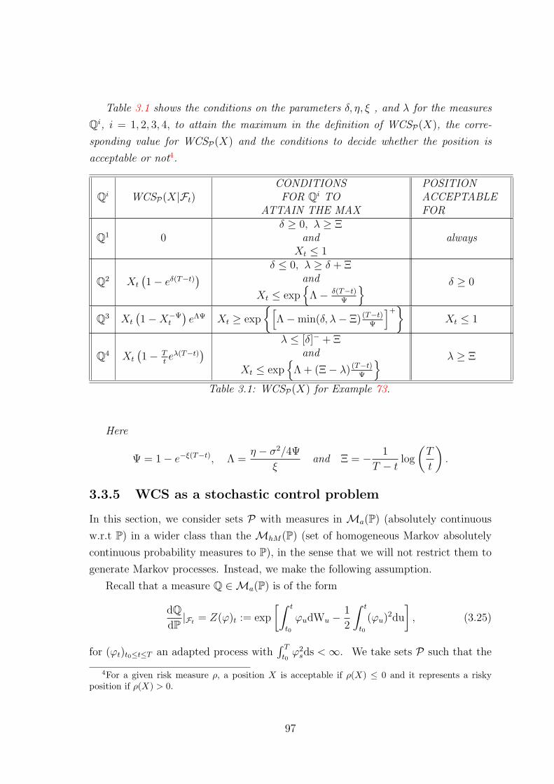
Table 3.1 shows the conditions on the parameters δ, η, ξ , and λ for the measures
Qi, i = 1, 2, 3, 4, to attain the maximum in the definition of WCSP(X), the corre-
sponding value for WCSP(X) and the conditions to decide whether the position is
acceptable or not4.
Qi WCSP(X|Ft)CONDITIONSFOR Qi TO
ATTAIN THE MAX
POSITIONACCEPTABLEFOR
Q1 0δ ≥ 0, λ ≥ Ξ
andXt ≤ 1
always
Q2 Xt
(1− eδ(T−t)
) δ ≤ 0, λ ≥ δ + Ξand
Xt ≤ exp
Λ− δ(T−t)Ψ
δ ≥ 0
Q3 Xt
(1−X−Ψ
t
)eΛΨ Xt ≥ exp
[Λ−min(δ, λ− Ξ) (T−t)
Ψ
]+Xt ≤ 1
Q4 Xt
(1− T
teλ(T−t)
) λ ≤ [δ]− + Ξand
Xt ≤ exp
Λ + (Ξ− λ) (T−t)Ψ
λ ≥ Ξ
Table 3.1: WCSP(X) for Example 73.
Here
Ψ = 1− e−ξ(T−t), Λ =η − σ2/4Ψ
ξand Ξ = − 1
T − tlog
(T
t
).
3.3.5 WCS as a stochastic control problem
In this section, we consider sets P with measures in Ma(P) (absolutely continuous
w.r.t P) in a wider class than the MhM(P) (set of homogeneous Markov absolutely
continuous probability measures to P), in the sense that we will not restrict them to
generate Markov processes. Instead, we make the following assumption.
Recall that a measure Q ∈Ma(P) is of the form
dQdP|Ft = Z(ϕ)t := exp
[∫ t
t0
ϕudWu −1
2
∫ t
t0
(ϕu)2du
], (3.25)
for (ϕt)t0≤t≤T an adapted process with∫ T
t0ϕ2
sds <∞. We take sets P such that the
4For a given risk measure ρ, a position X is acceptable if ρ(X) ≤ 0 and it represents a riskyposition if ρ(X) > 0.
97
set5
ΨP(P) :=
ϕt ∈ PM :
∫ T
t0
ϕ2sds <∞ and
dQdP|Ft = Z(ϕ)t as in (3.25) for Q ∈ P
is compact. This is, we make the following assumption:
Assumption 74 The set of priors P comes from a compact set of progressively mea-
surable and square integrable Girsanov kernels.
This assumptions is necessary for the solution of WCSP(X) using stochastic con-
trol theory (see [26]).
Assume the current time is t and we are interested in computing WCSP on a
position X for the risk horizon [t, t + θ], θ ≥ 0, where the process (Xt)0≤t≤T has
dynamics as in (Xt-SDE) under the measure P. Under Assumption 74, we can think
and work with the process Xt from the point of view of a controlled one-dimensional
SDE. In this case, the control variable ϕt only affects the drift term. Our controlled
SDE is given by
dXϕt =
b(Xϕ
t ) + a2(Xϕt )ϕt
dt + a(Xϕ
t )dWt.
And the problem of computing WCSP(X) is equivalent to
WCSP(X) = supQ∈P
EQ [−X]
= supϕ∈ΨP (P)
E [−Xϕ] .
Then using our assumptions on the drift function b, the volatility function a and
the fact that ΨP(P) is bounded, we apply usual arguments in stochastic control theory
(see [26, Chap. 6 p.155], [63, Chap. XI p.227] or [25, Chap. VI p.151]) to reduce
WCSP(X) to the solution of a nonlinear PDE of second order. This is described in
the following proposition.
Proposition 75 Let Xt be a Markov diffusion process on (Ω,F ,P) as in (Xt-SDE).
Let P satisfy the Assumption (74) and let ΨP(P) be the corresponding compact Gir-
sanov kernel set. For a risk horizon [t, t+ θ], θ ≥ 0, and the position X = Xt+θ−Xt,
WCSP(X) is given by
WCSP(X) = Xt − H(t,Xt)
5PM means progressively measurable process.
98
where H(t, x) is the solution of the following boundary value problem:
∂H
∂t+
1
2a2(x)
∂2H
∂x2+ b(x)
∂H
∂x+ sup
ϕ∈ΨP (P)
a2(x)ϕ
∂H
∂x
= 0, (τ, x) ∈ [t, t+ θ)× R,
H(t+ θ, x) = x.
As the set ΨP(P) is compact, the optimum ϕ∗ is attained. Then by a measurable
selection argument (see Appendix C) one can find a (measurable) function ϕ(t, x)
such that ϕ∗t = ϕ(t, x) for a.a. x.
The fact that the optimal control can be chosen as a measurable function only
on the current value of the process Xt means that the optimal control is Markov. In
this general setting, unfortunately the only thing we can say about the function ϕ is
that it is measurable, this is, it may not be even be differentiable as required in the
previous section.
3.4 Value-at-Risk (VaR)
In this section, we focus on the computation of VaR for processes given in (Xt-SDE).
Note that the definition of VaR in Definition 25 can be equivalently rewritten as
VaRα(X) = infm ∈ R : E[1−X≤m] ≥ 1− α.
This representation of VaR admits the following interpretation (see [48]):
“VaR is similar to finding the lowest strike price −m of a digital call option on the
position X under the probability P, such that its price is larger or equal than 1−α.”
Similarly to the WCS risk measure, the value of VaR can be characterised using
a PDE as shown in the next proposition.
Proposition 76 VaR-PDE. Let Xt be a Markov diffusion process on (Ω,F ,P) as
in (Xt-SDE). For the risk horizon [t, t + θ], θ > 0, and the position X = Xt+θ −Xt,VaRα(X) is given by
VaRα(X) = Xt − q+Xt+θ
(α) (3.26)
= Xt − sup q ∈ R : V q(t,Xt) ≤ α .
99
where V q(t, x) is the solution of the following boundary value problem:
Lb,a[V q](τ, x) = 0, (τ, x) ∈ [t, t+ θ)× R, (3.27)
V q(t+ θ, x) = 1x<q
for a fixed real number q and the operator Lb,a given by
Lb,a[·](t, x) =∂·∂t
+ b(x)∂·∂x
+1
2a(x)
∂2·∂x2
.
Proof. By the Markov property of the processXt, q+Xt+θ
(α) = sup q ∈ R : F (t,Xt; t+ θ, q) ≤ αwith F (t0, x0; t, x) the distribution function for the process Xt. Under our assump-
tions, F ∈ C1,2 in the back variables (t0, x0), so we can apply Ito’s formula and
characterise VaR as the solution of a PDE.
Remark 77 Let V (t, x, q) := V q(t, x) with V q be the solution of (3.27), the function
q 7−→ V (t, x, q) satisfy the properties of a distribution function, i.e.
1. The function V (t, x, q) is monotonic increasing and right continuous in q,
2. limq→∞
V (t, x, q) = 1 and limq→−∞
V (t, x, q) = 0.
3.5 Average Value-at-Risk (AVaR)
From the equivalence expressions of AVaRα in Proposition 29 and using the definition
of VaR in Definition 25, we have
AVaRα(X) = Xt − q+Xt+θ
(α) (3.28)
=1
αEP
[(q+Xt+θ
(α)−Xt+θ
)+]
+Xt − q+Xt+θ
(α) (3.29)
Then, AVaR can be interpreted as (see [48]):
“The price of a (standard European) put option with time to maturity θ with a
strike equal to the upper α-quantile of the position Xt+θ divided by the price of the
corresponding digital put option plus the actual value of the asset Xt minus the value
of the upper α-quantile of the position Xt+θ.”
This interpretation is useful for calculating AVaR when VaR is already known,
otherwise, one can compute it via a minimisation problem and recover VaR simulta-
neously. We refer to [93] for more details on this optimisation approach in a static
setting.
In a similar manner as WCS and VaR; AVaR can be computed as the solution to
a PDE as shown in the next proposition.
100
Proposition 78 . AVaR PDE Let Xt be a Markov diffusion process on (Ω,F ,P)
as in (Xt-SDE). For the risk horizon [t, t+θ], θ > 0, and the position X = Xt+θ−Xt,
AVaRα(X) is given by
AVaRα(X) =1
αU(t,Xt, q
+Xt+θ
(α)) +Xt − q+Xt+θ
(α). (3.30)
where U(t, x, q) := U q(t, x) and U q(t, x) is the solution of the following boundary value
problem:
Lb,a[U q](τ, x) = 0, (τ, x) ∈ (t, t+ θ)× R, (3.31)
U q(t+ θ, x) = [q − x]+,
for a fixed real number q and the operator Lb,a given by
Lb,a[·](t, x) =∂·∂t
+ b(t, x)∂·∂x
+1
2a(t, x)
∂2·∂x2
.
Proof. That AVaR is given by the solution of the PDE follows from the Markov
property of the process Xt.
In this section, we have characterised the computation for WCS, VaR and CVaR
via the solution of PDEs with final conditions. In most of the cases, we do not
expect the PDEs to have explicit solutions, but suitable numerical methods or series
expansion solutions can be applied to solve them. Whether the PDEs have explicit
solutions or not will depend strongly on the coefficients in the process Xt. If this is
the case, it means that one can compute explicitly the transition probability density
for the process Xt, as we will explore in the next section.
3.6 Computation of risk measures when the tran-
sition density is known
In this section, we show how to compute WCS, VaR and AVaR when the transition
probability density p(t, x; τ, y) for the process Xt on (Ω,F ,P) is known. At the end
of the section we present some examples.
3.6.1 WCS
We recall from Section 3.3.4 that for P ⊂ Mb,ahM(P) satisfying the Assumption 58,
we have a one-to-one correspondence between measures Qγ ∈ P and processes γ ∈ΥP . Furthermore, we also know from Proposition 70 that for each position X with
101
dynamics in (Xt-SDE) there exists a measure Q+ ∈ P and therefore a drift γ+(x) =
b(x) + a2(x)v+x (x) ∈ ΥP .
If we assume that the transition probability density p(t, x; τ, y) for the process Xt
on (Ω,F ,P) is known, and also the transition probability densities pγ(t, x; τ, y) for Xt
under each of the measures Qγ ∈ P , then WCS is related to pγ as follows.
From the definition of WCS and the equivalence relation in Remark 69, we have
WCSP(X) = supγ∈ΥP
EQγ [−X]
= Xt + supPγ∈P
∫R−pγ(t,Xt; t+ θ, y) y dy
= Xt −∫
Rpγ+
(t,Xt; t+ θ, y) y dy,
with pγ(t, x; τ, y) the transition probability density for the process Xt under the mea-
sure Pγ ∈ P .
From Lemma 64, the density process for Qγ ∈ P can be represented by
dQγ
dP|Fτ = Z (vγ(y))τ = ZH (V γ(y))τ =
V γ(Xτ )
V γ(Xt)exp
−∫ τ
t
Gb,ax [V γ](Xs)
V γ(Xs)ds
,
for V γ(y) = expvγ(y), so using the definition of Z•(t0, x0; t, x) in (3.15) evaluated
at the function v from (t, x) to (τ, y) we have
Zvγ(y)(t, x; τ, y) =V γ(y)
V γ(x)EP
[exp
−∫ τ
t
Gb,ax [V γ](Xs)
V γ(Xs)ds
|Xτ = y,Xt = x
].
Applying Proposition 66, we can compute explicitly the transition probability
density for Xt under Qγ ∈ P as
pγ(t, x; τ, y) = Zvγ(y)(t, x; τ, y) p(t, x; τ, y). (3.32)
The previous discussion suggests two alternatives to tackle the problem of com-
puting WCS when the transition probability density p(t, x; τ, y) for the process Xt on
(Ω,F ,P) is known. Each case will depend on the special situation on the dynamics
of Xt and the particular set P ⊂Mb,ahM(P).
Case 1: From the dynamics of Xt or directly from the set P we can deduce which
is the measure Q+ ∈ P that maximises the expected value. Then WCS will be
the expected value of the position −X under the measure Q+. We have seen
in Proposition 72 one alternative to compute the expected value via a PDE.
We give here another one using the transition probability density p(t, x; τ, y) as
follows:
102
1. Find the function f+(t, x) = u+(t) + v+(x) that defines the density
dQ+
dP|Ft = Z
(f+(t, x)
)t.
2. For V +(y) = expv+(y), compute the expected value
EP
[exp
−∫ τ
t
Gb,ax [V +](Xs)
V +(Xs)ds
|Xτ = y,Xt = x
].
3. Using (3.32), the transition probability density p+(t, x; τ, y) for the process
Xt under Q+ is
p+(t, x; τ, y) = Zv+(y)(t, x; τ, y) p(t, x; τ, y).
4. And the WCS will be given by
WCSP(X) = Xt −∫
Rpγ+
(t,Xt; t+ θ, y)ydy.
Case 2: We do not know the measure Q+ ∈ P , but we can compute
EP
[exp
−∫ τ
t
d(Xs)ds
|Xτ = y,Xt = x
]for
d(x) =Gb,a
x [V γ](x)
V γ(x)
and V γ, γ ∈ ΥP are the functions that define the density processes
dQγ
dP|Ft = LZ (V γ(x))t
for each Qγ ∈ P . In this case, the procedure to compute WCS using p(t, x; τ, y)
is as follows:
1. For each Qγ ∈ P , find V γ, γ ∈ ΥP such that
dQγ
dP|Ft = LZ (V γ(x))t .
2. Compute
EDγ(t, x; τ, y) := EP
[exp
−∫ τ
t
dγ(Xs)ds
|Xτ = y,Xt = x
]with dγ(x) = Gb,a
x [V γ ](x)V γ(x)
.
103
3. The transition probability density pγ(t, x; τ, y) for the process Xt under
Qγ ∈ P will be given by
pγ(t, x; τ, y) =V γ(y)
V γ(x)EDγ(t, x; τ, y) p(t, x; τ, y).
4. Compute
EV γ(t, x; θ) :=
∫R−pγ(t, x; t+ θ, y) y dy
5. The WCS will be given by
WCSP(X) = Xt + supγ∈ΥP
EV γ(t,Xt; θ).
3.6.2 VaR
In order to see how VaR can be expressed in terms of the transition probability density
p(t, x; τ, y) for the process Xt on (Ω,F ,P), define
V (t, x, I) :=
∫Rp(t, x; t+ θ, y)1Idy =
∫I
p(t, x; t+ θ, y)dy for I ⊂ B(R),
where B(R) is the Borel sigma-algebra on R. We can think of I as an interval on R.The function V (t, x, I) represents the conditional probability that Xt+θ belongs to a
given interval I for the information up to the time t. Similarly, we could have defined
it as
V (t, x, I) = P(Xt+θ ∈ I|Xt = x).
For m ∈ R take V (t, x,m) := V (t, x, I) with I = z : z < m; then using the
definition of VaRα in Definition 25 we have
VaRα(X) = Xt − q+Xt+θ
(α)
= Xt − supm ∈ R : E[1Xt+θ<m] ≤ α
= Xt − supm ∈ R : V (t,Xt, I) ≤ α with I = z : z < m
= Xt − supm ∈ R : V (t,Xt,m) ≤ α
= Xt − sup
m ∈ R :
∫y<m
p(t,Xt; t+ θ, y))dy ≤ α
.
Remark 79 For a general random variable X, if its distribution function f(x) has
no atoms and is continuous, the supremum on
sup
m ∈ R :
∫y<m
f(y) dy ≤ α
104
is attained at the value m∗ such that∫y<m∗
f(y) dy = α.
For an account of VaR and AVAR for general distributions see [72].
In our present setting, p(t, x; t + θ, y) is a continuous function and atom-less,
therefore we can express VaR for a position X as
VaRα(X) = Xt − q+Xt+θ
(α) = Xt −m∗
with m∗ obtained from the relation∫y<m∗
p(t, x; t+ θ, y))dy = α.
3.6.3 AVaR
We now describe how to express AVaR in terms of the transition probability density
p(t, x; τ, y) for the process Xt on (Ω,F ,P).
Define
U(t, x, q) ,∫
Rp(t, x; t+ θ, y) [q − y]+dy =
∫y6q
p(t, x; t+ θ, y)(q − y)dy for q ∈ R,
or equivalently
U(t, x, q) = EP[[q −Xt+θ]
+|Xt = x].
From the expression of AVaRα in (3.29) we have
AVaRα(X) =1
αEP
[(q+Xt+θ
(α)−Xt+θ
)+]
+ VaRα(X),
=1
αU(t, x, q+
Xt+θ(α)) + VaRα(X),
=1
α
∫n
y6q+Xt+θ
(α)o p(t,Xt; t+ θ, y)
(q+Xt+θ
(α)− y)
dy + VaRα(X),
= VaRα(Xt)−1
α
∫y60
p(t,Xt; t+ θ, y + q+
Xt+θ(α))ydy.
The computation of WCS, VaR and CVaR when there is available an explicit
expression for the transition probabilities p(t, x; τ, y) of the process Xt under the
appropriate measures is summarised in the following proposition.
105
Proposition 80 For a given set P ⊂Mb,ahM(P) satisfying Assumption 58, let p(t, x; τ, y)
(resp. pγ) be the transition probability density for a process Xt as in (Xt-SDE) under
P (resp. Pγ ∈ P). Then WCS, VaR and CVaR for the position X = Xt+θ −Xt can
be computed as follows:
WCSP(X) = Xt −∫ ∞
−∞pγ+
(t,Xt; t+ θ, y)ydy,
VaRα(X) = Xt − sup
m ∈ R :
∫ m
−∞p(t,Xt; t+ θ, y)dy ≤ α
,
CVaRα(X) = VaRα(X)− 1
α
∫ 0
−∞p(t,Xt; t+ θ, y + q+
Xt+θ(α))ydy.
Proof. Follows from previous discussion.
By the fact that p(t, x; τ, y) satisfies the Kolmogorov backward equation, it can be
checked directly that the expressions given above are the same as the ones obtained
using the PDE approach in sections 3.3, 3.4 and 3.5 given by the equations in (3.22),
(3.26) and (3.30), respectively. Note that in the expression for WCS, we need to know
the transition density function p+(t, x; τ, y) for the probability measures Q+ ∈ Pwhere the supremum in WCS is attained.
3.6.4 Example of risk measures for a single process
Example 81 (Geometric Brownian motion - Black-Scholes model.) Geometric
Brownian motion is one of the models most used in finance, and probably one of the
few processes that permits explicit computations. Fix θ > 0, and consider t to be the
current time and [t, t+ θ] the risk horizon. Assume we need to compute the risk of a
position Xθ = Xt+θ −Xt measured as WCS, VaR and CVaR, for Xt given by
dXt = µXtdt + σXtdWt.
In the notation in (Xt-SDE) we have b(x) = µx and a(x) = σx. The family of
functions
vδ(x) =
(δ − µ
σ2
)log(x), δ ∈ R
generates the family of drifts indexed by δ ∈ R given by γ(x) = δx that preserve
the Markov property and the structure of the model of having a linear drift. In this
case the corresponding density processes are well defined on (0,∞) (are uniformly
106
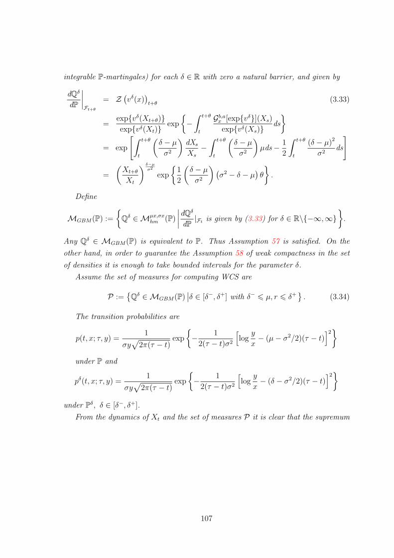
integrable P-martingales) for each δ ∈ R with zero a natural barrier, and given by
dQδ
dP
∣∣∣∣Ft+θ
= Z(vδ(x)
)t+θ
(3.33)
=expvδ(Xt+θ)expvδ(Xt)
exp
−∫ t+θ
t
Gb,ax [expvδ](Xs)
expvδ(Xs)ds
= exp
[∫ t+θ
t
(δ − µ
σ2
)dXs
Xs
−∫ t+θ
t
(δ − µ
σ2
)µds− 1
2
∫ t+θ
t
(δ − µ)2
σ2ds
]
=
(Xt+θ
Xt
) δ−µ
σ2
exp
1
2
(δ − µ
σ2
)(σ2 − δ − µ
)θ
.
Define
MGBM(P) :=
Qδ ∈Mµx,σx
hm (P)
∣∣∣∣dQδ
dP|Ft is given by (3.33) for δ ∈ R\−∞,∞
.
Any Qδ ∈ MGBM(P) is equivalent to P. Thus Assumption 57 is satisfied. On the
other hand, in order to guarantee the Assumption 58 of weak compactness in the set
of densities it is enough to take bounded intervals for the parameter δ.
Assume the set of measures for computing WCS are
P :=Qδ ∈MGBM(P)
∣∣δ ∈ [δ−, δ+] with δ− 6 µ, r 6 δ+. (3.34)
The transition probabilities are
p(t, x; τ, y) =1
σy√
2π(τ − t)exp
− 1
2(τ − t)σ2
[log
y
x− (µ− σ2/2)(τ − t)
]2under P and
pδ(t, x; τ, y) =1
σy√
2π(τ − t)exp
− 1
2(τ − t)σ2
[log
y
x− (δ − σ2/2)(τ − t)
]2under Pδ, δ ∈ [δ−, δ+].
From the dynamics of Xt and the set of measures P it is clear that the supremum
107
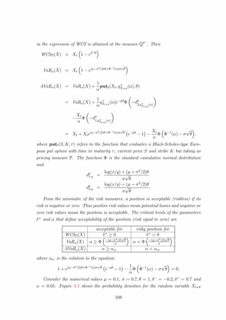
in the expression of WCS is attained at the measure Qδ+. Then
WCSP(X) = Xt
(1− eδ+θ
)VaRα(X) = Xt
(1− e(µ−σ2/2)θ+Φ−1(α)σ
√θ)
AVaRα(X) = VaRα(X) +1
αputP(Xt, q
+Xt+θ
(α), θ)
= VaRα(X) +1
αq+Xt+θ
(α)e−µθΦ
(−dµ
2,q+Xt+θ
(α)
)
−Xt
αΦ
(−dµ
1,q+Xt+θ
(α)
)
= Xt +Xte(µ−σ2/2)θ+Φ−1(α)σ
√θ(e−µθ − 1
)− Xt
αΦ(Φ−1(α)− σ
√θ).
where putP(S,K, τ) refers to the function that evaluates a Black-Scholes-type Euro-
pean put option with time to maturity τ , current price S and strike K but taking as
pricing measure P. The function Φ is the standard cumulative normal distribution
and
dµ1,q =
log(x/q) + (µ+ σ2/2)θ
σ√θ
dµ2,q =
log(x/q) + (µ− σ2/2)θ
σ√θ
.
From the axiomatic of the risk measures, a position is acceptable (riskless) if its
risk is negative or zero. Thus positive risk values mean potential losses and negative or
zero risk values mean the position is acceptable. The critical levels of the parameters
δ+ and α that define acceptability of the position (risk equal to zero) are
acceptable for risky position forWCSP(X) δ+ ≥ 0 δ+ < 0
VaRα(X) α ≥ Φ(−(µ−σ2/2)
√θ
σ
)α < Φ
(−(µ−σ2/2)
√θ
σ
)AVaRα(X) α ≥ αcr α < αcr
where αcr is the solution to the equation
1 + e(µ−σ2/2)θ+Φ−1(α)σ√
θ(e−µθ − 1
)− 1
αΦ(Φ−1(α)− σ
√θ)
= 0.
Consider the numerical values µ = 0.1, σ = 0.7, θ = 1, δ− = −0.2, δ+ = 0.7 and
α = 0.05. Figure 3.1 shows the probability densities for the random variable Xt+θ
108
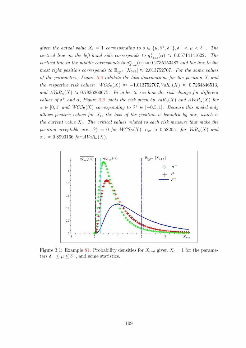
given the actual value Xt = 1 corresponding to δ ∈ µ, δ+, δ−, δ− < µ < δ+. The
vertical line on the left-hand side corresponds to q+Xt+θ
(α) ≈ 0.05714141622. The
vertical line in the middle corresponds to q+Xt+θ
(α) ≈ 0.2735153487 and the line to the
most right position corresponds to EQδ+ [Xt+θ] ≈ 2.013752707. For the same values
of the parameters, Figure 3.2 exhibits the loss distributions for the position X and
the respective risk values: WCSP(X) ≈ −1.013752707,VaRα(X) ≈ 0.7264846513,
and AVaRα(X) ≈ 0.7836260675. In order to see how the risk change for different
values of δ+ and α, Figure 3.3 plots the risk given by VaRα(X) and AVaRα(X) for
α ∈ [0, 1] and WCSP(X) corresponding to δ+ ∈ [−0.5, 1]. Because this model only
allows positive values for Xt, the loss of the position is bounded by one, which is
the current value Xt. The critical values related to each risk measure that make the
position acceptable are: δ+cr = 0 for WCSP(X), αcr ≈ 0.582051 for VaRα(X) and
αcr ≈ 0.8993166 for AVaRα(X).
Figure 3.1: Example 81. Probability densities for Xt+θ given Xt = 1 for the parame-ters δ− ≤ µ ≤ δ+, and some statistics.
109
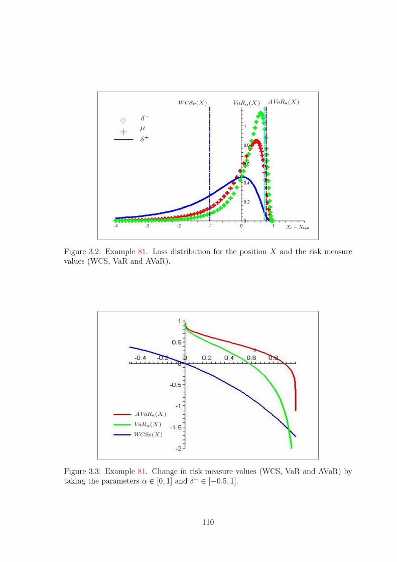
Figure 3.2: Example 81. Loss distribution for the position X and the risk measurevalues (WCS, VaR and AVaR).
Figure 3.3: Example 81. Change in risk measure values (WCS, VaR and AVaR) bytaking the parameters α ∈ [0, 1] and δ+ ∈ [−0.5, 1].
110
Chapter 4
Risk for Derivatives
4.1 Introduction
In this chapter, we study the problem of computing risk as WCS, VaR and AVaR for
derivative securities that depend on an underlying asset given by a Markov diffusion
processes as in the preceding chapter. This is, we assume that the derivative security
is defined by a positive function C(t, s) on the security St. Defining a process given
by
Xt = C(t, St),
one can apply Ito’s lemma to obtain the dynamics of X. Then our problem reduces
to the one studied in the previous chapter of computing the risk for the position X.
When the function C is not injective, the dynamics of the process Xt may degenerate.
In order to analyse this situation in detail, we look at the process Xt from the point
of view of a local transformation of the Markov diffusion process St. In particular, we
establish conditions and analyse when the transition probability density of a trans-
formed process Xt can be expressed in terms of the transition probability density of
our original process St. In other words, we find how to reduce the solution to the risk-
PDEs for the position X to the solution of a simpler PDEs problem corresponding to
the solution to the risk-PDEs for the position S.
We apply our results on local transformation of Markov diffusion processes to
the computation of risk for derivative securities and complement with examples. We
discuss briefly also the relation to this method with the approaches known as delta-
and delta-gamma approximation for the computation of risk of derivatives and the
case of American type-derivative securities.
111
4.2 Risk measures for European derivatives
Suppose the position X on (Ω,F ,P) of which we want to measure the risk is the
discounted net worth of a European-type contingent claim (derivative security) with
expiration time T and payoff function H(s) ≥ 0 on an underlying process St satisfying
the assumptions of Chapter 3 and given by
dSt = β(St)dt + α(St)dWt, with St = s. (S-SDE)
Assume the derivative security may not be liquidated during the risk horizon [t, t+θ],
for 0 < t ≤ t + θ < T . By the Markov property and our assumptions on the process
St the random variable Xt+θ may be written as a function C ∈ C1,2 of the process St
at time t+ θ, this is, Xt+θ = C(t+ θ, St+θ). Then, we can use Ito’s lemma to obtain
the dynamics of the process Xt and use the method in Chapter 3 to obtain the risk
of the position via the solution of the corresponding PDE. For the particular relation
between the process Xt and St we expect the corresponding risk PDEs to be related.
In this section, we focus on exploring the solution to the risk PDE for the derivative
security Xt in terms of the solution to the risk PDE for the underlying process St. In
order to set ideas in general rather than for a particular risk measure, we work from
the point of view of the transition probability densities (t.p.d.); that is, we explore
conditions for obtaining the t.p.d. of the derivative security Xt in terms of the t.p.d.
of the underlying process St. Once we have obtained the t.p.d. of Xt we can apply
the method in Section 3.6 for the computation of the risk of the position X measured
as WCSP(X), VaRα(X) and CVaRα(X).
4.2.1 The derivative-dynamics
In general, for a function C ∈ C1,2(R+ × R) define the process Xt = C(St, t). By
Ito’s lemma the dynamics of the process Xt (the C-dynamics) under the measure Pare given by
dXt = b(t, St)dt + a(t, St)dWt, with Xt = x = C(0, St), (4.1)
for
b(t, s) :=∂C
∂t(t, s) + β(t, s)
∂C
∂s(t, s) +
1
2α2(t, s)
∂2C
∂s2(t, s),
and
a(t, s) := α(t, s)∂C
∂s(t, s).
112
In particular, if C represents the current value of a European derivative security with
payoff function H(s) and risk-free rate r (we assume momentarily the risk-free rate
to be nonzero for completeness), then
C(t, St) = EQ[e−r(θ)H(St+θ)],
where Q is the risk-neutral probability measure. We can use the Black-Scholes equa-
tion for the derivative security to further simplify the expression for b(t, s) as
b(t, s) =∂C
∂t(t, s) + β(t, s)
∂C
∂s(t, s) +
1
2α2(t, s)
∂2C
∂s2(t, s)
= rC(t, s) + (β(t, s)− rs)∂C
∂s(t, s).
In particular, assuming r = 0 we have
b(t, s) = β(t, s)∂C
∂s(t, s).
Remark 82 If there exist points (t, x) in the domain of the function C at which∂C∂x
(t, s) = 0, then they have to be analysed carefully as they may induce degeneracy
in the process Xt = C(t, St). On the other hand, when the process Xt is regarded as
a local change of variable transformation of the process St, then the analysis of the
degeneracy points is similar to analysing what happen to a transformed process when
the transformation is not injective. For that purpose, we borrow some results on the
transformation of continuous Markov diffusions developed in [8]. In order to make
this thesis self-contained, we recall all the results and proofs needed in the next section
and we adapt them to the present context.
4.2.2 Homogeneous local transformations
For completeness and in order to introduce ideas, before we analyse the case of C(t, St)
as a local transformation of the St process, we study what happen with local trans-
formations that do not depend on time (homogeneous). For that purpose, we recall
some key results that guarantee the Markov property for the transformed processes.
Lemma 83 Images of a Markov process. [from [71, Ex.1.17 p.87]] Let X be a
Markov process with transition function (Pt) and φ a Borel function from (E, E) into
a space (E, E) such that φ(A) ∈ E for every A ∈ E. If moreover, for every t and every
A ∈ EPt,x(φ
−1(A)) = Pt,x(φ−1(A)) whenever φ(x) = φ(x),
then the process Yt = φ(Xt) under Pt,x, x ∈ E, is a Markov process with state space
(E, E).
113
In order for a transformed Markov process to be again Markov, it is necessary that
the conditional probability on the points where the transformation is not injective is
well defined. This is, if two different points have the same image, then the conditional
probability starting at any of those points of the inverse image of any event in the
space must be equal. As we are interested in compute the t.p.d. of a transformed
process in terms of the t.p.d. of the original process, the next corollary is an adapted
version of the lemma above (see also [33, Theorem 271J, p. 343]).
Corollary 84 Let St be a Markov diffusion process as in (S-SDE) with conditional
probability Pt,s(·) := P(·|St = s) and denote by pS(t, s; t+θ, z) its transition probability
density. For a differentiable function C : R → R the process Xt = C(St) is also a
Markov process if either of the following conditions hold:
1. C is a diffeomorphism on R. In this case, the transition probability density of
the transformed process Xt under P is given by
pX(t, x; t+ θ, y) =
∣∣∣∣∣(dC
ds(χ(y))
)−1∣∣∣∣∣ pX(t, χ(x); t+ θ, χ(y))
with χ(x) the corresponding inverse function of C(s) such that C(χ(x)) = x.
2. For D ⊆ dom[C] (the domain of the function C) with |Dc| = 0 ( or equivalently
L(s ∈ D) = 1, and L the Lebesgue measure), the derivative of C does not vanish
for each s ∈ D and there exist a disjoint sequence of Borel sets (Dk)k∈N with
union D, such that C Dk (C restricted to the set Dk) is injective for every
k ∈ N. And furthermore, for every t and F ⊂ R we have that
Pt,s(C−1(F )) = Pt,s(C
−1(F )) whenever C(s) = C(s). (4.2)
In this case, the transition probability density of the transformed process Xt
under P is given by
pX(t, x; t+θ, y) =
∑∞k=0
∣∣∣(dCds
(χ(y)))−1∣∣∣ pS(t, χ(x); t+ θ, χ(y)) for y ∈ C(Dk ∩ dom[pS])
0 for y ∈ R\C(Dk)
with χ(x) the corresponding inverse function of C(s) such that C(χ(x)) = x.
Proof. Note that Part 1 is a special case of Part 2. To prove Part 2 observe that
we may allow the derivative of C to vanish on the sets Dk\Dk (boundary of Dk) for
k ∈ N. In such case, take D′ = s ∈ D|∂C∂s
(s) = 0 and E = D\D′. Clearly D′ is a
114

null set, therefore we still have L(s ∈ E) = 1, E =⋃∞
k=0Dk and C Dk is injective
for each k ∈ N.
If C is differentiable relative to its domain at every s ∈ E, then C is continuous,
Borel measurable, so C(St) is a well defined random variable.
Fix k ∈ N and F ⊆ R, define the functions
gk(y) =
∑∞k=0
∣∣∣(dCds
(χ(y)))−1∣∣∣ pS(t, χ(x); t+ θ, χ(y)) for y ∈ C(Dk ∩ dom[pS])
0 for y ∈ R\C(Dk)
then pS(t, s; t+ θ, z) = |dCds
(z)|gk(C(z)) for every z ∈ Dk
⋂dom[pS], and we have∫
F
gkdP =
∫C(Dk)
gkIFdP =
∫Dk
∣∣∣∣dCds (s)
∣∣∣∣ gk(C(s))IF P(ds)
=
∫Dk∩C−1(F )
fdP = P(s ∈ Dk ∩ C−1(F )).
Now summing over k and by the fact that each gk is non-negative for each k, g =∑∞k=0 gk is finite almost everywhere on F , and∫
F
gdP =∞∑
k=0
∫F
gkdP =∞∑
k=0
P(s ∈ Dk ∩ C−1(F )) = P(s ∈ C−1(F )).
Now, applying the same reasoning but with conditional probabilities to the event
St = s, and by the condition
Pt,s(C−1(F )) = Pt,s(C
−1(F )) whenever C(s) = C(s)
we have that
Pt,s(s ∈ C−1(F )) = Pt,s(C(s) ∈ F ).
As F was arbitrary, then g is the density function for C(s) as needed.
The condition (4.2) in the Corollary 84 above may be a very restrictive one. To
give an idea of this restrictiveness, consider the following proposition saying that the
only valid homogeneous local trasnformations of Brownian motion (that satisfy the
condition in (4.2)) are functions that are either invertible in all the real line, or are
functions that are symmetric with respect to a vertical line crossing at the points
where the the function is not injective (e.g. sin(x), cos(x), etc.).
Proposition 85 Let St, 0 ≤ t < ∞ be a Brownian motion on (Ω,F ,P) starting at
s > 0 for t ∈ R. Then C is a change of variable transformations (Xt = C(St))
satisfying conditions in Corollary 84 if and only if
115

1. C is invertible in all its domain, or
2. C is a symmetric function.
Before we give the proof, we need a somehow trivial but useful result.
Lemma 86 For a1, b1, a2, b2 ∈ R, the equation
Φ[b1 + h]− Φ[a1 + h] + Φ[b2 + h]− Φ[a2 + h] = Φ[b1]− Φ[a1] + Φ[b2]− Φ[a2] (4.3)
has nontrivial solution h ∈ R only in any of the following cases:
1. if a = a1 = a2 and b = b1 = b2, then h = −(a+ b),
2. if a1 + b1 = a2 + b2 then h = −(a1 + b1),
3. if a1 + b2 = a2 + b1 then h = −(a1 + b2).
And Φ is the standard cumulative normal distribution.
Remark 87 That h = −(a + b) satisfies the relation in (4.3) is very intuitive, it is
perhaps surprising that it is the unique solution, therefore we decided to include a
proof.
Proof of Lemma 86. For the Part 1, we need to prove that h = −(a + b)
is the only solution to Φ[b + h] − Φ[a + h] = Φ[−a] − Φ[−b] for a, b ∈ R. Define
f(h) = Φ[b+ h]−Φ[a+ h] =∫ b+h
a+h1√2π
exp−y2
2dy. It is direct to see that f(h) > 0,
continuous for all h ∈ R and limh→−∞ f(h) = 0 = limh→∞ f(h) with derivative
f ′(h) = 1√2π
[exp− (b+h)2
2 − exp− (a+h)2
2]. And the only point satisfying f ′(h) = 0
is h∗ = − (b+a)2
with f ′′(h∗) < 0, then h∗ is a maximum point for f(h). All this
together leads to the conclusion that f is increasing in (−∞, h∗) and decreasing in
(h∗,∞). Therefore for any α ∈ R, α 6= f(h∗), there exist real numbers h1 6= h2 such
that α = f(h1) = f(h2). In particular, if h∗ 6= 0, there exist a unique real number h
with the property f(0) = f(h).
Now, in order to compute h note that f ′(h∗ −∆) = −f ′(h∗ + ∆) for any ∆ > 0,
so the function f is symmetric. And for ∆ = h∗ we have f ′(0) = −f ′(2h∗), so our
natural candidate is h = 2h∗ = −(a+ b), which is confirmed to be the right choice by
the fact that f”(0) = f”(h) and f(0) = f(h).
Parts 2 and 3 result from applying Part 1 to all different combinations of terms
in (4.3).
116

Proof of Proposition 85. The first characterisation is obvious from Part 1 of
Corollary 84. For the second one, assume without loss of generality that C has a
unique minimum point at s∗ and that is decreasing in (−∞, s∗) and increasing in
(s∗,∞). Take F = s ∈ R : α 6 s 6 β for α, β ∈ R, so C−1(F ) = s ∈ R : s′β 6
s 6 s′α and sα 6 s 6 sβ. Then condition (4.2) is equivalent to check whether P1 is
equal to P2 for:
P1 = P[s′β 6 St 6 s′α|St0 = s0
]+ P [sα 6 St 6 sβ|St0 = s0]
P2 = P[s′β 6 St 6 s′α|St0 = s′0
]+ P [sα 6 St 6 sβ|St0 = s′0]
with s0 and s′0 such that C(s0) = C(s′0). But by properties of Brownian motion we
have
P1 = P[s′β − s0√t− t0
6 ξ 6s′α − s0√t− t0
]+ P
[sα − s0√t− t0
6 ξ 6sβ − s0√t− t0
]= Φ
[s′α − s0√t− t0
]− Φ
[s′β − s0√t− t0
]+ Φ
[sβ − s0√t− t0
]− Φ
[sα − s0√t− t0
]P2 = P
[s′β − s0√t− t0
+ h 6 ξ 6s′α − s0√t− t0
+ h
]+ P
[sα − s0√t− t0
+ h 6 ξ 6sβ − s0√t− t0
+ h
]= Φ
[s′α − s0√t− t0
+ h
]− Φ
[s′β − s0√t− t0
+ h
]+ Φ
[sβ − s0√t− t0
+ h
]− Φ
[sα − s0√t− t0
+ h
]with ξ = St−s0√
t−t0∼ N (0, 1) (N (0, 1) is the standard normal distribution and Φ the
standard cumulative normal distribution) and h =s0−s′0√
t−t0. Then by Lemma 86 we
have two possibilities in comparing P1 and P2
1.
h = −s′α + s′β√t− t0
+2s0√t− t0
= −sβ + sα√t− t0
+2s0√t− t0
and from here, the condition turns into s′0 = (s′α +s′β)−s0 = (sβ +sα)−s0. But
this can not be true because, taking s0 =(sβ+sα)
2we would have s′0 = s0 meaning
that(sβ+sα)
2< s∗ is a minimum point, contradicting the initial assumption that
s∗ is the unique minimum.
2.
h = −s′α + sα√t− t0
+2s0√t− t0
= −sβ − s′β√t− t0
+2s0√t− t0
and the condition turns into s′0 = (s′α + sα)− s0 = (sβ + s′β)− s0. Considering
the last two equalities we have s′α − s′β = sβ − sα meaning that both intervals
have to be of the same length. Now for s0 = s′α+sα
2+ ∆ we need s′0 = s′α+sα
2−∆
and this indicates that the function has to be symmetric around s′α+sα
2, this is,
s∗ = s′α+sα
2=
sβ+s′β2
.
117
4.2.3 The process C(t, St) as a local transformation of the St
process
In this section, we study the dynamics of the process Xt as a local change of variable
transformation of the process St, defined as follows.
Definition 88 Let St be a Markov diffusion process as in S-SDE. A local change of
variable transformation is a map C : [t, t+ θ]× R −→ R.
In the case the transformation C(t, s) is injective on s for all t ∈ [t, t + θ], the
t.p.d. of the process Xt can be easily recovered from the t.p.d. of the process St as
shown in the next proposition.
4.2.3.1 Injective local transformations
Proposition 89 Let St be a Markov diffusion process as in (S-SDE) with conditional
probability Pt,s(·) := P(·|St = s) and denote by pS(t, s; t+θ, z) its transition probability
density with t < t+ θ. For an injective differentiable function C : [t, t+ θ]× R → Rthe process Xt = C(t, St) is also a Markov process with transition probability density
under P given by
pX(t, x; t+ θ, y) =
∣∣∣∣∣(∂C
∂s(t+ θ, χ(t+ θ, y))
)−1∣∣∣∣∣ pS(t, χ(t, x); t+ θ, χ(t+ θ, y))
with χ(t, x) the corresponding inverse function of C(t, s) such that C(t, χ(t, x)) = x.
Proof. The proof is very similar to the first part in the homogeneous case.
A direct application to the above proposition concerns the computation of the
upper α-quantile of derivative securities whose values are strictly increasing (resp.
strictly decreasing) functions on the current level of the underlying process St. Then
using these results, one can easily compute VaR for positions in derivative securities
with the help of the results in Section 3.4.
Corollary 90 Let C be a local change of variable transformation with C(t, ·) contin-
uous and strictly increasing function. Then
q+C(t+θ,St+θ)(α) = C(t, q+
St+θ(α)).
If C(t, ·) is a continuous strictly decreasing function, then
q+C(t+θ,St+θ)(α) = C(t, q+
St+θ(1− α)).
118
Proof. This is a direct consequence of using Proposition 89 to find the t.p.d. for
the transformed processes Xt and the application of the method in Section 3.6 for
computing q+• (1− α).
Remark 91 Most of the common derivative securities and some simple exotic deriva-
tives satisfy the assumptions in the above proposition, for example: plain vanilla calls
and puts, common barrier options, etc.
In order to fix ideas, consider the following example.
Example 92 (VaRα of a down-and-out call) Assume St is given by a geometric
Brownian motion
dSt = rStdt + σStdWt
absorbed at a level s ≥ B > 0. The t.p.d.of the process St for t < τ is given by (see
Example 5 in [8] )
p(t, s; τ, z) = pGBM(r,σ)(t, s; τ, z)−( sB
)1−2r/σ2
pGBM(r,σ)
(B2
s, t; z, τ
).
Assume the current time is t and we want to measure the VaR of a position on a
down-and-out European call option with strike K, maturity T and barrier B < K for
the risk horizon [t, T ], T < T . The price of the down-and-out call option cd/o(t, St) is
an increasing function on St and given by
cd/o(t, St) = c(t, St, K, T )−(St
B
)1−2r/σ2
c
(t,B2
St
, K, T
),
with c(t, St, K, T ) denoting the price of a European call option with strike K, and
maturity T . In order to apply Corollary 90, we need first to compute q+ST
(1 − α).
Define for m ∈ [B,∞)
ym = −log(
St
m
)+ (r − 1/2σ2) (T − t)
σ√T − t
,
and for y ∈ [yB,∞)
Σ(y) := Φ (y) +
(St
B
)1−2r/σ2
Φ
(−y −
2 log(
St
B
)σ√T − t
), (4.4)
with Φ the standard cumulative Normal distribution.
119
The function Σ(y) is strictly increasing on [yB,∞) with αmin := Σ(yB) and
Σ(∞) = 1. Thus using the t.p.d. for the process St we conclude that
q+ST
(α) =
B if α ≤ αmin
m∗(α) α > αmin
with m∗(α) given by
m∗(α) = exp
Σ−1(α)σ√T − t+ log(St) +
(r − 1/2σ2
)(T − t)
. (4.5)
Note that Σ−1(α) has not explicit expression but it can easily be computed numerically.
And the quantity αmin has the interpretation of the probability of hitting the barrier
B.
For simplicity in the computations, consider r = 0. The case r 6= 0 can be treated
similarly with minor changes.
Then using Proposition 26 and Corollary 90 for computing VaRα on a long position
in the derivative security (a down-and-out call) we have
VaRα(cd/o(T, ST )− cd/o(t, St)) = cd/o(t, St)− q+C(T,ST )(α)
= cd/o(t, St)− cd/o(t, q+ST
(α))
=
cd/o(t, St) if α ≤ αmin
cd/o(t, St)− cd/o(t,m∗(α)) α > αmin.
Then the position will be acceptable when α ≤ αmin only if St = B. And if α > αmin
we have that the position in the derivative is acceptable if
cd/o(t, St) ≤ cd/o(t,m∗(α)),
or equivalently,
St ≤ m∗(α).
In order to see acceptability in terms of α ∈ (0, 1), define αSt := Σ(St), using (4.4)
or (4.5) one can easily see show that
αSt = Σ
(1/2σ2(T − t)
σ√T − t
).
Then the position on the derivative will be acceptable if α ≥ αSt.
120
The VaRα of a short position in the derivative is
VaRα(−cd/o(T, ST ) + cd/o(t, St)) = −cd/o(t, St)− q+−C(T,ST )(α)
= −cd/o(t, St)− cd/o(t, q+ST
(1− α))
=
−cd/o(t, St) if 1− α ≤ αmin
−cd/o(t, St)− cd/o(t,m∗(1− α)) 1− α > αmin.
In this case, the short position in the down-and-out call will always be acceptable.
4.2.3.2 Piecewise injective transformations
In this section, we consider the situation where there may exist points (t, s) on the do-
main of the local transformation C at which ∂C∂s
(t, s) = 0. This is, the transformation
is not injective on the whole domain of C.
As one of our motivating applications is to be able to find explicit expressions for
the t.p.d. when C(t, s) represents the price of a European derivative security on a
risky asset given by continuous Markov diffusion process, we expect C to be a nice
behaving function. The next proposition shows that if the set of critical points given
by ∂C∂s
(t, s) = 0 is a curve (or several disjoint curves), then we are able to solve as in
the previous section.
Proposition 93 Consider C ∈ C1,2 ([0, T ]× R) and for t ∈ [t, t+ θ],
1. [CONTINUITY CONDITION I] if there is s∗ ∈ R such that
∂C
∂s(t, s∗) = 0 and
∂2C
∂s2(t, s∗) 6= 0,
then there exists an interval [t, t+∆t], with 0 < ∆t ∈ R+ and a unique function
sm : [t, t + ∆t] → R such that sm(t) = s∗ and ∂C∂s
(τ, sm(τ)) = 0 for all τ ∈[t, t+ ∆t). Furthermore,
2. [CONTINUITY CONDITION II] if there exists a process St on (Ω,F ,P) sat-
isfying the Assumptions 55 and 56 given by the sde in (S-SDE), and func-
tions Ψ,Φ, and k satisfying the conditions in the Feynman-Kac theorem for the
stochastic representation
C(t, s) = EQ
[Ψ(ST )Λ(t) +
∫ t+θ
t
Φ(υ, Sυ)Λ(t)dυ|St = s
], (4.6)
with Λ(t) = exp−∫ t+θ
tk(θ, Sθ)dθ
and Q a measure equivalent to P. Then
sm(τ) and its derivative dsm
dt(τ) are continuous for all t 6 τ 6 t+ θ.
121
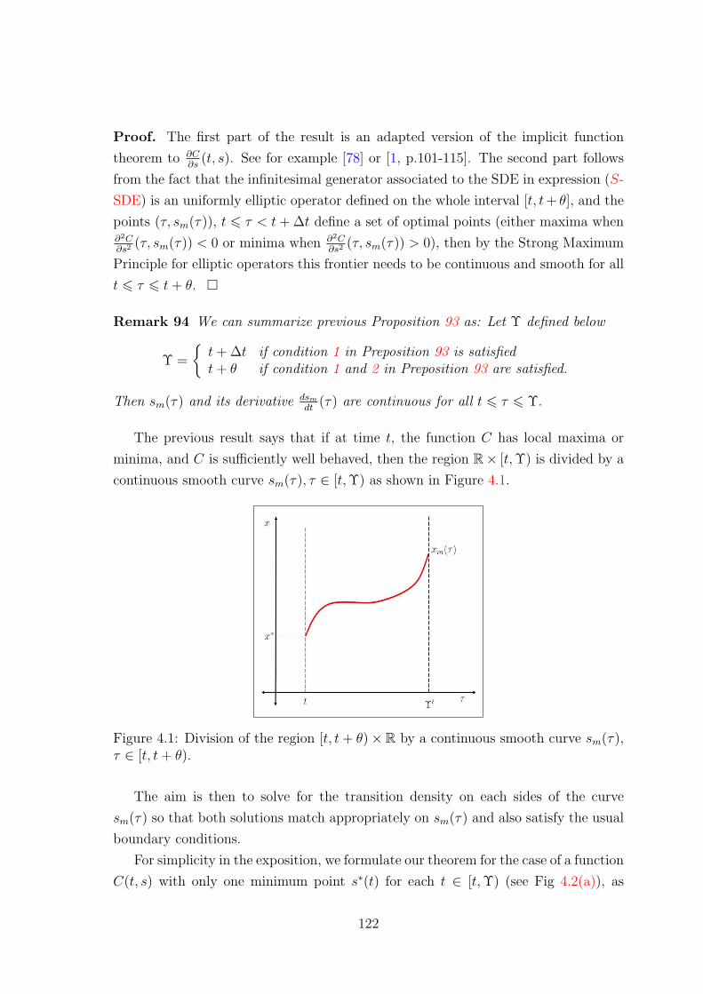
Proof. The first part of the result is an adapted version of the implicit function
theorem to ∂C∂s
(t, s). See for example [78] or [1, p.101-115]. The second part follows
from the fact that the infinitesimal generator associated to the SDE in expression (S-
SDE) is an uniformly elliptic operator defined on the whole interval [t, t+ θ], and the
points (τ, sm(τ)), t 6 τ < t+ ∆t define a set of optimal points (either maxima when∂2C∂s2 (τ, sm(τ)) < 0 or minima when ∂2C
∂s2 (τ, sm(τ)) > 0), then by the Strong Maximum
Principle for elliptic operators this frontier needs to be continuous and smooth for all
t 6 τ 6 t+ θ.
Remark 94 We can summarize previous Proposition 93 as: Let Υ defined below
Υ =
t+ ∆t if condition 1 in Preposition 93 is satisfiedt+ θ if condition 1 and 2 in Preposition 93 are satisfied.
Then sm(τ) and its derivative dsm
dt(τ) are continuous for all t 6 τ 6 Υ.
The previous result says that if at time t, the function C has local maxima or
minima, and C is sufficiently well behaved, then the region R× [t,Υ) is divided by a
continuous smooth curve sm(τ), τ ∈ [t,Υ) as shown in Figure 4.1.
Figure 4.1: Division of the region [t, t+ θ)×R by a continuous smooth curve sm(τ),τ ∈ [t, t+ θ).
The aim is then to solve for the transition density on each sides of the curve
sm(τ) so that both solutions match appropriately on sm(τ) and also satisfy the usual
boundary conditions.
For simplicity in the exposition, we formulate our theorem for the case of a function
C(t, s) with only one minimum point s∗(t) for each t ∈ [t,Υ) (see Fig 4.2(a)), as
122
generalisations may be treated similarly (e.g. several local minima (resp. maxima)
or when minima (resp. maxima) appear in time). See Example 99: Inhomogeneous
transformations of BM.
The extension of Corollary 84 to the inhomogeneous case is considered in the next
proposition.
For simplicity in the notation, in the following proposition consider the risk horizon
to be [t0, t], corresponding to the pairs (t0, x0) and (t, x).
Proposition 95 Let St be a Markov process on (Ω,F ,P) given by
dSt = b(t, St)dt + a(t, St)dWt with St0 = s0
satisfying the Assumptions 55 and 56, and a function C ∈ C1,2([t0, t]×R) satisfying the
conditions in Proposition 93, with a unique minimal point s∗(t) for each t ∈ [t0,Υ).
Write s∗ := s∗(t0). Denote by pX(t0, x0; t, x) the transition probability density for the
process Xt = C(t, St) under P and define the function φt,x for x0 = C(t0, s0) as
φt,x(t0, x0) = pX(t0, x0; t, x).
For fixed t < Υ and x, φt,x satisfies the final condition backward equation
Lβ,α[φt,x](τ, x0) = 0, (τ, x0) ∈ (t0, t)× R, (4.7)
limτt
φt,x(τ, x0) = δ(y0 − y), y ∈ R. (4.8)
with
β(t, s) = Lb,a[C](t, s) and α(t, s) = a(t, s)∂C
∂s(t, s).
Then solving for φt,x in the above system is equivalent to solve for Ψt,s in
Lb,aΨt,s(τ, s0) = 0, (τ, s0) ∈ [t0, t]× R
limτt
Ψt,s(τ, s0) = δ(s0 − s) + δ(s0 − s),
Ψ(τ, sm(τ)) = δ(sm(τ)− s) for all τ ∈ [t0, t],
with s 6 sm(t) 6 s such that C(t, s) = x = C(t, s), and δ(z − x) is the delta function
of z centred at x. Furthermore, if for arbitrary I ⊂ R the following condition holds∫C−1(t,I)
Ψt,s(t0, s0)ds =
∫C−1(t,I)
Ψt,s(t0, s0)dx whenever C(t, s0) = C(t, s0),
(4.9)
123
then pS(t0, s0; t, s) = Ψt,s(t0, s0) is the transition probability density for the process St
under P and pX and pS are related as follows
pX(t0, x0; t, x) =
∣∣∣(∂C
∂s(t, χl(t, x))
)−1∣∣∣ pS(t0, χ(t0, x0); t, χ
l(t, x))
+∣∣∣(∂C∂x
(t, χr(t, x)))−1∣∣∣ pS(t0, χ(t0, y0); t, χ
r(t, x))
for x ≥ C(t, sm(t))
with
χ(t0, x0) =
χl(t0, x0) if s0 ≤ sm(t0)χr(t0, x0) if s0 > sm(t0)
for χl(t, x) ≤ sm(t) ≤ χr(t, x) representing the inverse functions of C(t, s), i.e.,
C(t, χl(t, x)) = x = C(t, χr(t, x)), and the function sm(τ) is the time parametrisation
of a curve where ∂C∂s
(τ, sm(τ)) = 0 for τ ∈ [t0, t] and sm(t0) = s∗. For details see the
proof below.
The proof is similar in spirit at the one for the homogeneous case, plus considering
the conditions in Proposition 93 for guaranteeing the differentiability and continuity
of the degeneracy points. We prove this time the result from a PDE point of view.
Proof. As the proof is long, we divide it into four parts:
We will omit the supraindices in Ψ and φ, replace (t0, s0) by (τ, ς) and (t0, x0) by
(τ, ξ) for simplicity in the notation.
1. Continuation of the solving region: As the assumptions in Proposition 93
are satisfied, there exist a differentiable and continuous function sm : R+ → R+
such that sm(τ) = s∗ and ∂C∂s
(τ, sm(τ)) = 0 for all τ < Υ.
2. Equation reduction via change of variable Define
Γ = (τ, sm(τ)) : τ < Υ
On Γ, note that
β(τ, ς) =∂C
∂τ+
1
2a(τ, ς)2∂
2C
∂ς2and α(τ, ς) = 0.
Take Ψ(τ, ς) = φ(τ, ξ) = φ(τ, C(τ, ς)) then we have
∂Ψ
∂τ=∂φ
∂τ+∂C
∂τ
∂φ
∂ς,
∂Ψ
∂ς=∂C
∂ς
∂φ
∂ξ= 0
and∂2Ψ
∂ς2=
(∂C
∂ς
)2∂φ
∂ξ2+∂2C
∂ς2∂φ
∂ξ=∂2C
∂ς2∂φ
∂ξ
124
and as ∂C∂s
(τ, sm(τ)) = 0, equation (4.7) reduces to
∂Ψ
∂t+
1
2a(τ, ς)2∂
2Ψ
∂s2+ b(τ, ς)
∂Ψ
∂s= 0.
Using the fact that sm(τ) for τ ∈ [t0, t] is a minimal point for C, as illustrated
in Figure 4.2(a), the expression in (4.8) becomes
limτt
Ψ(τ, ς) = δ(ξ − x) = δ(C(τ, ς)− C(t, s)) = δ(ς − s) + δ(ς − s)
for s 6 sm(t) 6 s such that C(t, s) = x = C(t, s). But if s = sm(t) then
s = sm(t) = s. Thus
limτt
Ψ(τ, ς) = δ(sm(t)− s).
In particular, if condition 2 in Proposition 93 is satisfied, then
β(τ, ς) =0 = α(τ, ς)
(as ∂u∂t
+ 12a(τ, ς)2 ∂2C
∂s2 + b(τ, ς)∂C∂s
= −a(τ, ς)2 hx
h∂C∂s
with h(t, St) a P-martingale),
then the Equation (4.7) remains
∂Ψ
∂t(τ, sm(τ)) = 0 for all τ ∈ [t0, t), t < T with Ψ(t) = δ (xm(t)− s) ,
which implies that
Ψ(τ) =δ (sm(τ)− s) for all τ ∈ [t0, t], for t < T .
In order to solve the PDE in (4.7) not including Γ, define
D := R+ × R\Γ
and take
Cr(τ, ς) =
C(τ, ς) if s > sm(t)0 else
and C l(τ, ς) =
C(τ, ς) if s < sm(t)0 else
.
Then in D we have C(τ, ς) = C l(τ, ς) + C l(τ, ς) with C l and Cr invertible
functions, therefore the following change of variable
Ψ(τ, ς) = φ(τ, ξ) = φ(t, C(τ, ς))
is well defined, and using the properties of change of variable transformation,
the first part of the equation in (4.7) is transformed into
Lb,aΨ(τ, ς) = LLb,a[C],a ∂C∂x [φ](τ, ξ) = 0, (τ, ς) ∈ ×[t0, t)× R,
125

and the final condition remains
limτt
Ψ(τ, ς) = δ(C(t, ς)− x), x ∈ R,
which for s 6 sm(t) 6 s such that C(t, s) = x = C(t, s) the final condition
above can be rewritten as
limτt
Ψ(τ, ς) = δ(C(τ, ς)− x) = δ(ς − s) + δ(ς − s).
3. Solution to the related problems Summarising the steps above, solving
equation (4.7) is equivalently to solve the following problem
Lb,aΨ(τ, ς) = 0, (τ, ς) ∈ ×[t0, t)× R (4.10)
limτt
Ψ(τ, ς) = δ(ς − s) + δ(ς − s),
Ψ(τ, sm(τ)) = δ(sm(τ)− s) for all τ ∈ [t0, t].
But the above system in (4.10) can be split into two problems as:
Ψ(τ, ς) = Ψl(τ, ς) + Ψr(τ, ς)
with Ψl(τ, ς) and Ψr(τ, ς) solutions of
Lb,aς Ψl(τ, ς) = 0, τ ∈ [t0, t) for ς 6 sm(τ)
limτt
Ψl(τ, ς) = δ(ς − s)
Ψl(τ, sm(τ)) = δ(sm(τ)− s) for all τ ∈ [t0, t].
and
Lb,aΨr(τ, ς) = 0, τ ∈ ×[t0, t) for ς > sm(τ)
limτt
Ψr(τ, ς) = δ(ς − s)
Ψr(sm(τ), τ) = δ(sm(τ)− s) for all τ ∈ [t0, t].
and using the stochastic representation formula we have that
Ψl(τ, ς) = pS(τ, ς; t, s) with ς 6 sm(τ) for all τ ∈ [t0, t]
Ψr(τ, ς) = pS(τ, ς; t, x) with ς > sm(τ) for all τ ∈ [t0, t].
Therefore
Ψr(τ, ς) = pS(τ, ς; t, s)Iς≤sm(t) + pS(τ, ς; t, x)Ism(t)<ς
126

4. Back transformation of variables. Now, transforming back into (t, x) vari-
ables, note that
Ψ(τ, ς) = pX(τ, C(τ, ς); t, x) = pS(τ, ς; t, s)Iς≤sm(t) + pS(τ, ς; t, s)Ism(t)<ς,
with s = χr(t, x), s = χl(t, x) and for
ς = χ(τ, ξ) =
χl(τ, ς) if ς ≤ sm(τ)χr(τ, ς) if ς > sm(τ)
(4.11)
with χl(t, x) ≤ sm(t) ≤ χr(t, x) representing the inverse functions Cr and C l
defined above in (4.11), i.e., Cr(t, χr(t, x)) = x = C l(t, χl(t, x)), as illustrated
in Fig. 4.2(b). Using similar arguments as in Proposition 84 we get the desired
expression
pX(t0, x0; t, x) =
∣∣∣(∂C
∂s(t, χl(t, x))
)−1∣∣∣ pS(t0, χ(t0, x0); t, χ
l(t, x))
+∣∣∣(∂C∂s
(t, χr(t, x)))−1∣∣∣ pS(t0, χ(t0, x0); t, χ
r(t, x))
for x ≥ C(t, sm(t)).
127
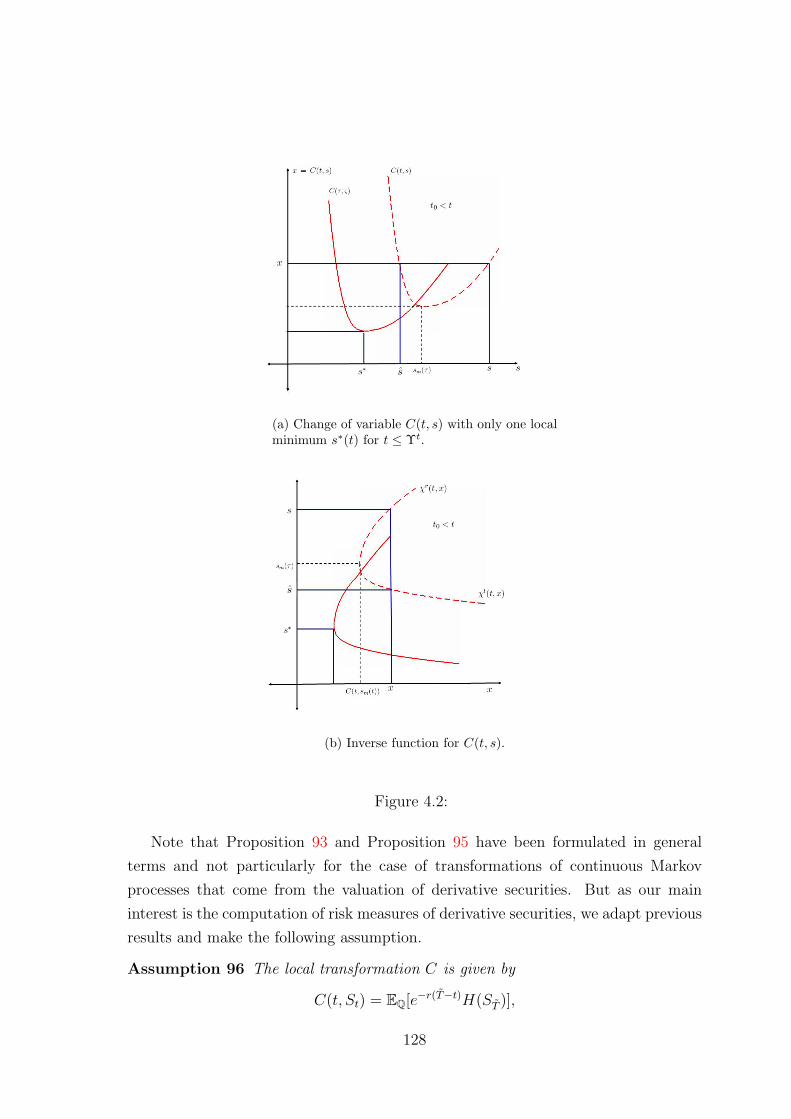
(a) Change of variable C(t, s) with only one localminimum s∗(t) for t ≤ Υt.
(b) Inverse function for C(t, s).
Figure 4.2:
Note that Proposition 93 and Proposition 95 have been formulated in general
terms and not particularly for the case of transformations of continuous Markov
processes that come from the valuation of derivative securities. But as our main
interest is the computation of risk measures of derivative securities, we adapt previous
results and make the following assumption.
Assumption 96 The local transformation C is given by
C(t, St) = EQ[e−r(T−t)H(ST )],
128
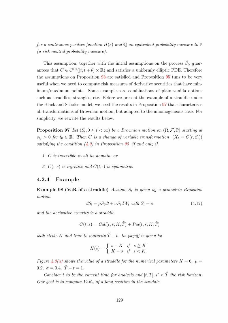
for a continuous positive function H(s) and Q an equivalent probability measure to P(a risk-neutral probability measure).
This assumption, together with the initial assumptions on the process St, guar-
antees that C ∈ C1,2([t, t+ θ]× R) and satisfies a uniformly elliptic PDE. Therefore
the assumptions on Proposition 93 are satisfied and Proposition 95 tuns to be very
useful when we need to compute risk measures of derivative securities that have min-
imum/maximum points. Some examples are combinations of plain vanilla options
such as straddles, strangles, etc. Before we present the example of a straddle under
the Black and Scholes model, we need the results in Proposition 97 that characterises
all transformations of Brownian motion, but adapted to the inhomogeneous case. For
simplicity, we rewrite the results below.
Proposition 97 Let (St, 0 ≤ t <∞) be a Brownian motion on (Ω,F ,P) starting at
st0 > 0 for t0 ∈ R. Then C is a change of variable transformation (Xt = C(t, St))
satisfying the condition (4.9) in Proposition 95 if and only if
1. C is invertible in all its domain, or
2. C(·, s) is injective and C(t, ·) is symmetric.
4.2.4 Example
Example 98 (VaR of a straddle) Assume St is given by a geometric Brownian
motion
dSt = µStdt + σStdWt with St = s (4.12)
and the derivative security is a straddle
C(t, s) = Call(t, s;K, T ) + Put(t, s;K, T )
with strike K and time to maturity T − t. Its payoff is given by
H(s) =
s−K if s ≥ KK − s if s < K.
Figure 4.3(a) shows the value of a straddle for the numerical parameters K = 6, µ =
0.2, σ = 0.4, T − t = 1.
Consider t to be the current time for analysis and [t, T ], T < T the risk horizon.
Our goal is to compute VaRα of a long position in the straddle.
129
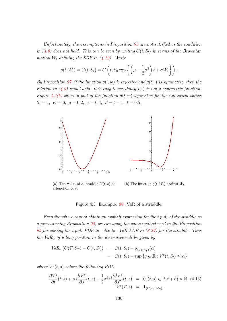
Unfortunately, the assumptions in Proposition 95 are not satisfied as the condition
in (4.9) does not hold. This can be seen by writing C(t, St) in terms of the Brownian
motion Wt defining the SDE in (4.12). Write
g(t,Wt) = C(t, St) = C
(t, S0 exp
(µ− 1
2σ2
)t+ σWt
).
By Proposition 97, if the function g(·, w) is injective and g(t, ·) is symmetric, then the
relation in (4.9) would hold. It is easy to see that g(t, ·) is not a symmetric function.
Figure 4.3(b) shows a plot of the function g(t, w) against w for the numerical values
St = 1, K = 6, µ = 0.2, σ = 0.4, T − t = 1, t = 0.5.
(a) The value of a straddle C(t, s) asa function of s.
(b) The function g(t, Wt) against Wt.
Figure 4.3: Example: 98. VaR of a straddle.
Even though we cannot obtain an explicit expression for the t.p.d. of the straddle as
a process using Proposition 95, we can apply the same method used in the Proposition
95 for solving the t.p.d. PDE to solve the VaR-PDE in (3.27) for the straddle. Thus
the VaRα of a long position in the derivative will be given by
VaRα (C(T, ST )− C(t, St)) = C(t, St)− q+C(T,ST )(α)
= C(t, St)− sup q ∈ R : V q(t, St) ≤ α
where V q(t, s) solves the following PDE
∂V q
∂t(t, s) + µs
∂V q
∂s(t, s) +
1
2σ2s2∂
2V q
∂s2(t, s) = 0, (t, s) ∈ [t, t+ θ)× R, (4.13)
V q(T, s) = 1C(T,s)<q.
130

The function C(t, s) satisfies the elliptic PDE (Black-Scholes equation with r = 0)
∂C
∂t(t, s) +
1
2σ2s2∂
2C
∂s2(t, s) = 0, (τ, s) ∈ [t, T )× R,
C(T , s) = H(s),
and ∂C∂s
(τ,K) = 0 with ∂2C∂s2 (τ,K) 6= 0 for all t 6 τ 6 T . The function sm : [t, T ] →
R defined as
sm(t) = K with∂C
∂s(τ, sm(τ)) = 0 for all τ ∈ [t, T ),
is continuous with continuous derivative dsm
dt(τ). As in Proposition 95, we write the
function C as the sum of two injective functions C(t, s) = Cr(t, s) + C l(t, s) with
Cr(t, s) = Call(t, s;K, T ) and C l(t, s) = Put(t, s;K, T ).
Take
ym(t) = log
(sm(t)
K
), yl
q = log
((C l)−1(q)
K
), yr
q = log
((Cr)−1(q)
K
),
and by the usual dimensionalisation and change of variable to reduce the PDE in
(4.13) to the heat equation, take
s = Key, t = T − 2τ/σ2 and uq(τ, y) = exp ηy + βτV q
(T − 2τ
σ2, Key
).
Taking
η = −k − 1
2, β = −
(k − 1
2
)2
and k =2µ
σ2,
the PDE becomes
uqτ = uq
yy for −∞ < y <∞ (4.14)
with the initial condition
uq(0, y) := u0(y) = 1C(T,s)<q =
e−ηy for yl
q < y < yrq
0 else, q > C(t,K)
and the moving boundary condition
uq(τ, y) = 0 for q = C
(T − 2τ
σ2, K
)and for all τ ∈ [0, T − t].
Due to the condition above we need to use the method of images to solve the
equation in (4.14). Solving and substituting back we have
slq = Keyl
q = (C l)−1(q),
srq = Keyr
q = (Cr)−1(q),
131

and
V q(t, s) = Φ(dµ2,sr
q)− Φ(dµ
2,slq),
with Φ the standard cumulative normal distribution and
dµ2,E =
log(St/E) + (µ− σ2/2)(T − t)
σ√T − t
.
One can easily check that choosing q such that q = qα := q+C(T,ST )(α) we have
C l(t, Sl
qα
)= qα = Cr
(t, Sl
qα
),
and
srq = q+
ST(δ + α) and sl = q+
ST(α)
for 0 ≤ δ + α ≤ 1 with
q+ST
(α) = s exp(µ− σ2/2)(T − t) + Φ−1(δ)σ√T − t,
then we have V q(t, s) = α. Thus
q+C(T,ST )(α) = C(t, q+
ST(δ)),
for δ satisfying the equality
C(t, q+ST
(α)) = C(t, q+ST
(δ + α)). (4.15)
Therefore the VaRα of a long position in the derivative is
VaRα(C(T, ST )− C(t, St)) = C(t, St)− C(t, q+ST
(δ))
= C(t, St)− C(t, St exp(µ− σ2/2)(T − t) + Φ−1(δ)σ√T − t)
with δ satisfying (4.15).
This is, we need to find δ and α such that DIF (δ, α) = 0 for
DIF (δ, α) := C(t, q+ST
(δ), K, T )− C(t, q+ST
(δ + α), K, T ).
By the shape of the function C(t, S), it is direct to see that there exist values of 0 ≤ δ ≤1 and 0 ≤ α ≤ 1 such that the function DIF (δ, α) takes the value zero. We illustrate
this fact with some numerical values for St = 1, K = 6, µ = 0.2, σ = 0.4, T − t = 1,
Figure 4.4(a) exhibits the value of the function DIF (δ, α) for α = 0.01, and Figure
4.4(b) plots the values of DIF (δ, α) for α = 0.05, 0.1 and 0.2.
For the value α = 0.01, the corresponding values in δ ≈ 0.0882971, which gives the
values q+C(T,ST )(α) = C(t, q+
ST(δ)) ≈ 1.708133948, and VaRα(C(T, ST ) − C(t, St)) ≈
13.291866787
132
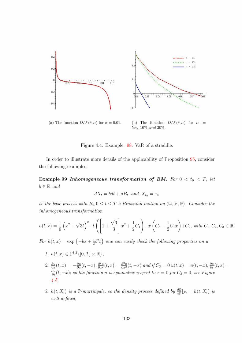
(a) The function DIF (δ, α) for α = 0.01. (b) The function DIF (δ, α) for α =5%, 10%, and 20%.
Figure 4.4: Example: 98. VaR of a straddle.
In order to illustrate more details of the applicability of Proposition 95, consider
the following examples.
Example 99 Inhomogeneous transformation of BM. For 0 < t0 < T , let
b ∈ R and
dXt = bdt+ dBt and Xt0 = x0
be the base process with Bt, 0 ≤ t ≤ T a Brownian motion on (Ω,F ,P). Consider the
inhomogeneous transformation
u(t, x) =1
6
(x2 +
√3t)2
−t
([1 +
√3
3
]x2 +
1
2C1
)−x(C3 −
1
2C1x
)+C2, with C1, C2, C3 ∈ R.
For h(t, x) = exp−bx+ 1
2b2t
one can easily check the following properties on u
1. u(t, x) ∈ C1,2 ([0, T ]× R) ,
2. ∂u∂x
(t, x) = −∂u∂x
(t,−x), ∂2u∂x2 (t, x) = ∂2u
∂x2 (t,−x) and if C3 = 0 u(t, x) = u(t,−x), ∂u∂t
(t, x) =∂u∂t
(t,−x); so the function u is symmetric respect to x = 0 for C3 = 0, see Figure
4.5,
3. h(t,Xt) is a P-martingale, so the density process defined by dQdP |Ft = h(t,Xt) is
well defined,
133
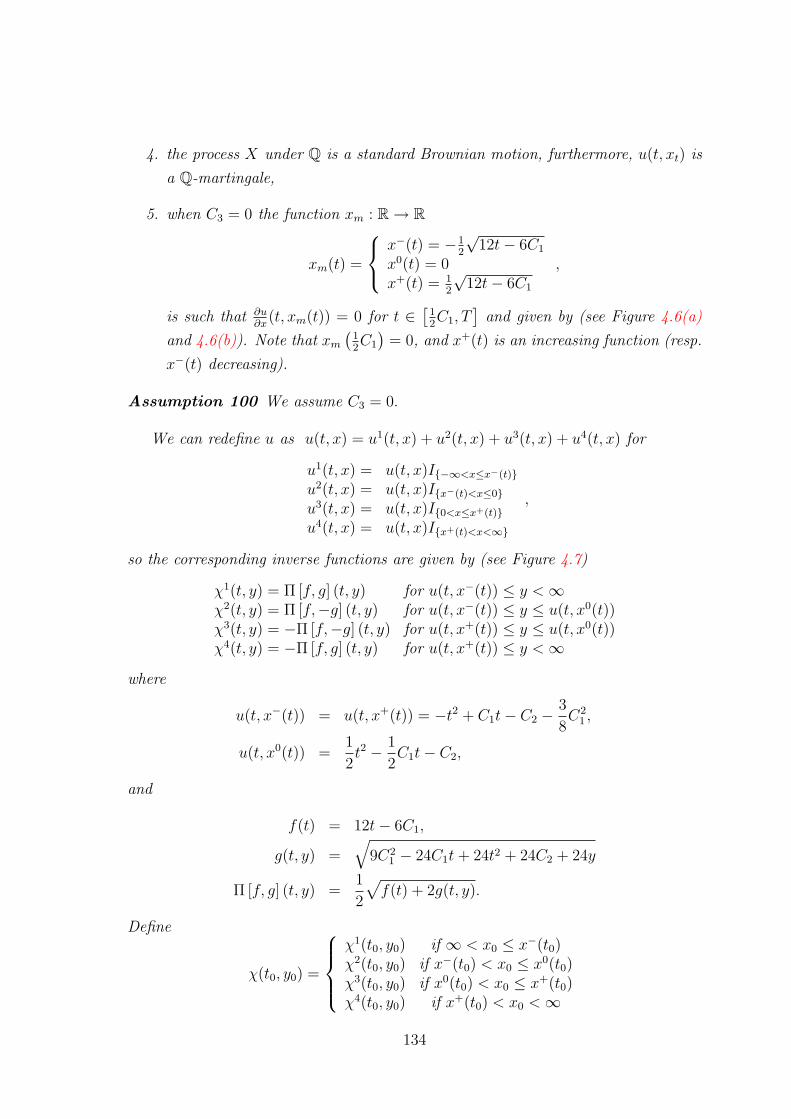
4. the process X under Q is a standard Brownian motion, furthermore, u(t, xt) is
a Q-martingale,
5. when C3 = 0 the function xm : R → R
xm(t) =
x−(t) = −1
2
√12t− 6C1
x0(t) = 0x+(t) = 1
2
√12t− 6C1
,
is such that ∂u∂x
(t, xm(t)) = 0 for t ∈[
12C1, T
]and given by (see Figure 4.6(a)
and 4.6(b)). Note that xm
(12C1
)= 0, and x+(t) is an increasing function (resp.
x−(t) decreasing).
Assumption 100 We assume C3 = 0.
We can redefine u as u(t, x) = u1(t, x) + u2(t, x) + u3(t, x) + u4(t, x) for
u1(t, x) = u(t, x)I−∞<x≤x−(t)u2(t, x) = u(t, x)Ix−(t)<x≤0u3(t, x) = u(t, x)I0<x≤x+(t)u4(t, x) = u(t, x)Ix+(t)<x<∞
,
so the corresponding inverse functions are given by (see Figure 4.7)
χ1(t, y) = Π [f, g] (t, y) for u(t, x−(t)) ≤ y <∞χ2(t, y) = Π [f,−g] (t, y) for u(t, x−(t)) ≤ y ≤ u(t, x0(t))χ3(t, y) = −Π [f,−g] (t, y) for u(t, x+(t)) ≤ y ≤ u(t, x0(t))χ4(t, y) = −Π [f, g] (t, y) for u(t, x+(t)) ≤ y <∞
where
u(t, x−(t)) = u(t, x+(t)) = −t2 + C1t− C2 −3
8C2
1 ,
u(t, x0(t)) =1
2t2 − 1
2C1t− C2,
and
f(t) = 12t− 6C1,
g(t, y) =√
9C21 − 24C1t+ 24t2 + 24C2 + 24y
Π [f, g] (t, y) =1
2
√f(t) + 2g(t, y).
Define
χ(t0, y0) =
χ1(t0, y0) if ∞ < x0 ≤ x−(t0)χ2(t0, y0) if x−(t0) < x0 ≤ x0(t0)χ3(t0, y0) if x0(t0) < x0 ≤ x+(t0)χ4(t0, y0) if x+(t0) < x0 <∞
134
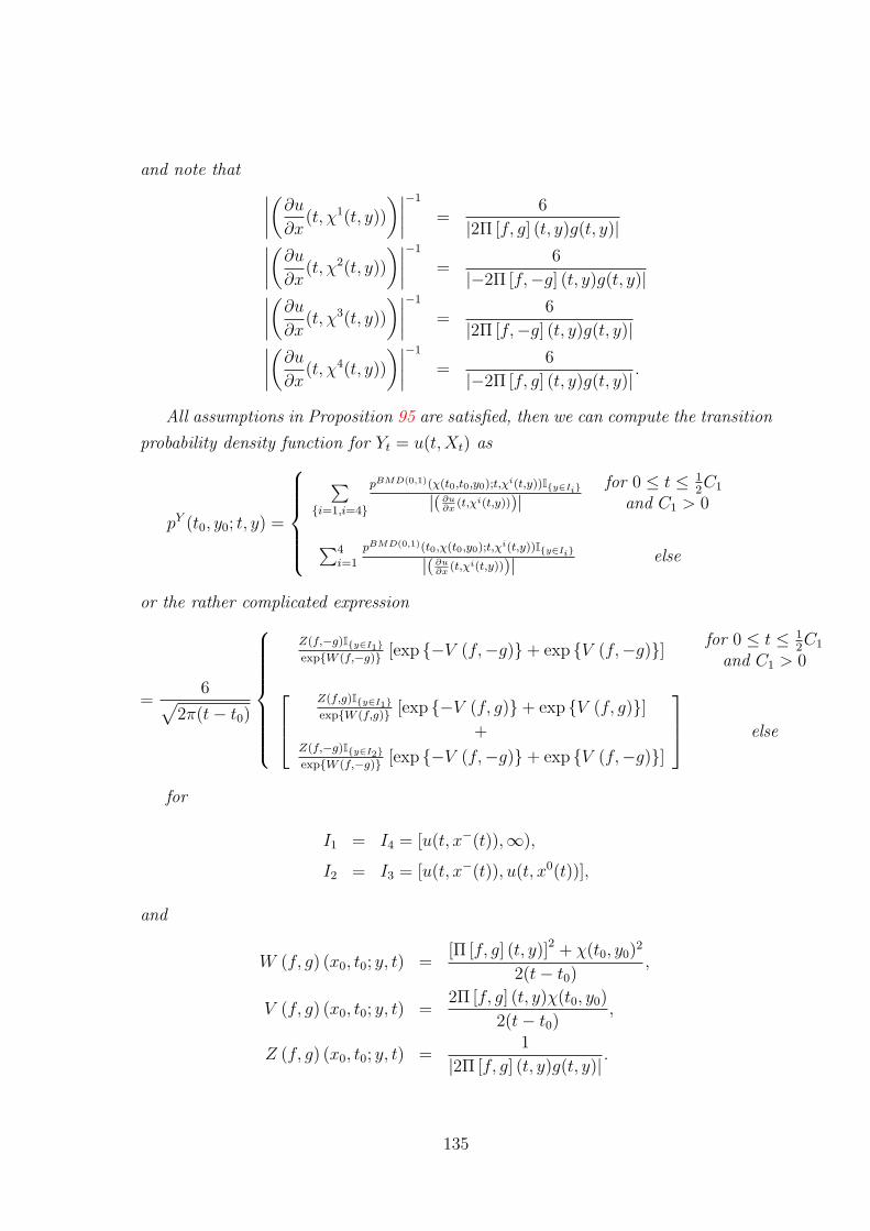
and note that ∣∣∣∣(∂u∂x(t, χ1(t, y))
)∣∣∣∣−1
=6
|2Π [f, g] (t, y)g(t, y)|∣∣∣∣(∂u∂x(t, χ2(t, y))
)∣∣∣∣−1
=6
|−2Π [f,−g] (t, y)g(t, y)|∣∣∣∣(∂u∂x(t, χ3(t, y))
)∣∣∣∣−1
=6
|2Π [f,−g] (t, y)g(t, y)|∣∣∣∣(∂u∂x(t, χ4(t, y))
)∣∣∣∣−1
=6
|−2Π [f, g] (t, y)g(t, y)|.
All assumptions in Proposition 95 are satisfied, then we can compute the transition
probability density function for Yt = u(t,Xt) as
pY (t0, y0; t, y) =
∑
i=1,i=4
pBMD(0,1)(χ(t0,t0,y0);t,χi(t,y))Iy∈Ii
|( ∂u∂x
(t,χi(t,y)))|for 0 ≤ t ≤ 1
2C1
and C1 > 0
∑4i=1
pBMD(0,1)(t0,χ(t0,y0);t,χi(t,y))Iy∈Ii
|( ∂u∂x
(t,χi(t,y)))| else
or the rather complicated expression
=6√
2π(t− t0)
Z(f,−g)Iy∈I1expW (f,−g) [exp −V (f,−g)+ exp V (f,−g)] for 0 ≤ t ≤ 1
2C1
and C1 > 0Z(f,g)Iy∈I1expW (f,g) [exp −V (f, g)+ exp V (f, g)]
+Z(f,−g)Iy∈I2expW (f,−g) [exp −V (f,−g)+ exp V (f,−g)]
else
for
I1 = I4 = [u(t, x−(t)),∞),
I2 = I3 = [u(t, x−(t)), u(t, x0(t))],
and
W (f, g) (x0, t0; y, t) =[Π [f, g] (t, y)]2 + χ(t0, y0)
2
2(t− t0),
V (f, g) (x0, t0; y, t) =2Π [f, g] (t, y)χ(t0, y0)
2(t− t0),
Z (f, g) (x0, t0; y, t) =1
|2Π [f, g] (t, y)g(t, y)|.
135

To see that this is indeed a transition probability function, one can easily check
that
∫R
∣∣∣∣(∂u∂x(t, χi(t, y))
)∣∣∣∣−1
pBMD(0,1)(t0, χ(t0, y0); t, χi(t, y))Iy∈Iidy =
−Ξ + 1
2i = 1
Ξ i = 2Ξ i = 3
−Ξ + 12
i = 4
and Ξ a real number, so∫
R p(t0, y0; t, y)dy = 1 (in the particular case 0 ≤ t ≤12C1, C1 > 0 the terms for i = 2, 3 vanish and Ξ = 0 ).
136
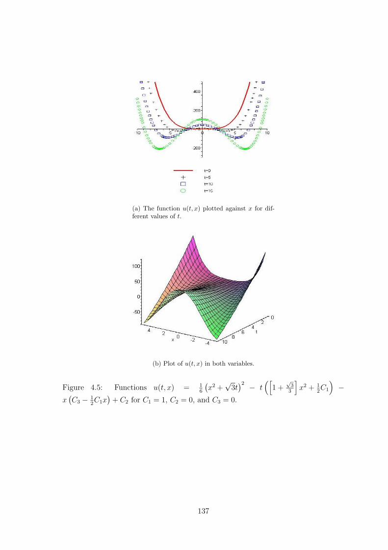
(a) The function u(t, x) plotted against x for dif-ferent values of t.
(b) Plot of u(t, x) in both variables.
Figure 4.5: Functions u(t, x) = 16
(x2 +
√3t)2 − t
([1 +
√3
3
]x2 + 1
2C1
)−
x(C3 − 1
2C1x
)+ C2 for C1 = 1, C2 = 0, and C3 = 0.
137
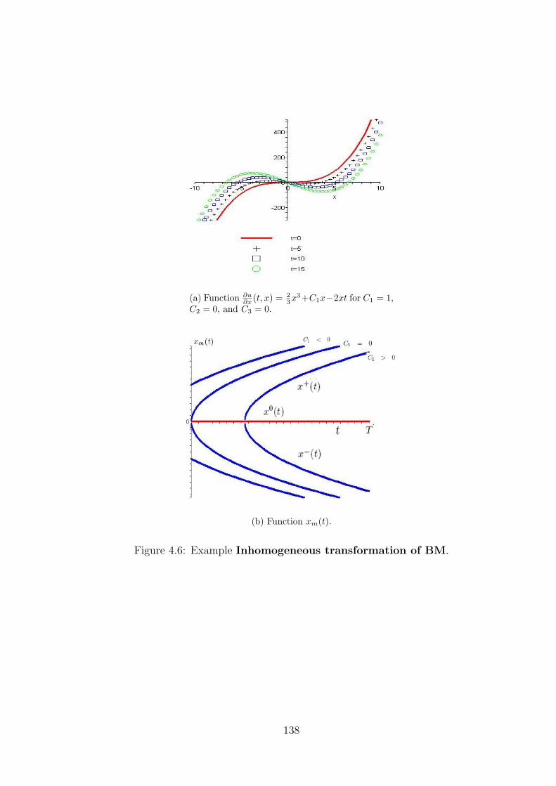
(a) Function ∂u∂x (t, x) = 2
3x3+C1x−2xt for C1 = 1,C2 = 0, and C3 = 0.
(b) Function xm(t).
Figure 4.6: Example Inhomogeneous transformation of BM.
138
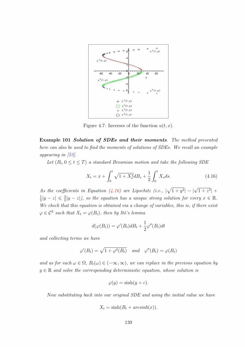
Figure 4.7: Inverses of the function u(t, x).
Example 101 Solution of SDEs and their moments. The method presented
here can also be used to find the moments of solutions of SDEs. We recall an example
appearing in [53].
Let (Bt, 0 ≤ t ≤ T ) a standard Brownian motion and take the following SDE
Xt = x+
∫ t
0
√1 +X2
sdBs +1
2
∫ t
0
Xsds. (4.16)
As the coefficients in Equation (4.16) are Lipschitz (i.e., |√
1 + y2| − |√
1 + z2| +12|y − z| 6 3
2|y − z|), so the equation has a unique strong solution for every x ∈ R.
We check that this equation is obtained via a change of variables, this is, if there exist
ϕ ∈ C2 such that Xt = ϕ(Bt), then by Ito’s lemma
d(ϕ(Bt)) = ϕ′(Bt)dBt +1
2ϕ′′(Bt)dt
and collecting terms we have
ϕ′(Bt) =√
1 + ϕ2(Bt) and ϕ′′(Bt) = ϕ(Bt)
and as for each ω ∈ Ω, Bt(ω) ∈ (−∞,∞), we can replace in the previous equation by
y ∈ R and solve the corresponding deterministic equation, whose solution is
ϕ(y) = sinh(y + c).
Now substituting back into our original SDE and using the initial value we have
Xt = sinh(Bt + arcsinh(x)).
139
In order to find the n-th moment for Xt, and as the function sinh(y) is a diffeomor-
phism of R, as shown in Figure 4.8, we can use Part 1 of Corollary 84 (homogeneous
diffeomorphism) to find its transition probability density and then its n-th moment.
Thus,
pX(t0, x0; t, x) =1√
2π(x2 + 1)(t− t0)exp
− [arcsinh(x)− arcsinh(x0)]
2
2(t− t0)
and
E[Xnt |Xt0 = x0] =
∫ ∞
−∞xnpX(t0, x0; t, x)dx
=
∫ ∞
−∞
xn√2π(x2 + 1)(t− t0)
exp
− [arcsinh(x)− arcsinh(x0)]
2
2(t− t0)
dx
=
∫ ∞
−∞
1
2n√
2π(t− t0)(exp2U − 1)n exp
− U2
2(t− t0)− nU
dU
for U = log
(y+√
y2+1
y0+√
y20+1
), expanding the power, calculating the integrals and collecting
terms the expression remains
E[Xnt |Xt0 = x0] = lim
y→∞A(n, t, t0)
n∑i=0
(−1)i
(ni
)exp 2i(i− n)(t− t0)C(n, t, t0, i, y, y0)
=1
2nexp
n2(t− t0)
2
n∑i=0
(−1)i
(ni
)exp 2i(i− n)(t− t0) (4.17)
with
A(n, t, t0) =1
2nexp
n2(t− t0)
2
B(n, t, t0, i, y, y0) =
log
(y+√
y2+1
y0+√
y20+1
)− (n− 2i)(t− t0)
√t− t0
C(n, t, t0, i, y, y0) = Φ [B(n, t, t0, i, y, y0)]− Φ [B(n, t, t0, i,−y, y0)]
as limy→∞C(n, t, t0, i, y, y0) = 1 and Φ the standard cumulative normal distribution
function.
Denote by
Θni , (−1)i
(ni
)exp 2i(i− n)(t− t0)
1
2nexp
n2(t− t0)
2
,
we can further simplify Equation (4.17) using the following remarks:
140
• For n an odd number (n = 2k + 1)
The sum in Equation (4.17) has an even number of terms (n+ 1 = 2k + 2)
Θ2k+12(k−j)+1 < 0 for j = 0 . . . k
Θ2k+12(k−j) > 0 for j = 0 . . . k
Θ2k+12k+1−j = −Θ2k+1
j for j = 0 . . . k
by the above properties we find that
2k+1∑j=0
Θ2k+12k+1−j =
k∑j=0
Θ2k+12k+1−2j +
k∑j=0
Θ2k+12k−2j = −
k∑j=0
Θ2k+12j +
k∑j=0
Θ2k+12j = 0.
• For n an odd number (n = 2k)
The sum in Equation (4.17) has an odd number of terms (n+ 1 = 2k + 1)
Θ2k2(k−j)−1 < 0 for j = 0 . . . k
Θ2k2(k−j) > 0 for j = 0 . . . k
Θ2k2k−j = Θ2k
j for j = 0 . . . k
the following relation holds:
Θ2kj + Θ2k
j+1 = Υ(k, j) for j = 0 . . . k
for Υ(k, j) , Θ2kj
1− (n−j)
(j+1)exp [2(2j − n+ 1)(t− t0)]
.
Then, the expression in Equation (4.17) simplifies to
E[Xnt |Xt0 = x0] =
1 for n = 00 for n = 2k + 1
2∑m−1
i=0 Υ(k, i) + Θ2kk for n = 2k and k = 2m
2∑m−1
i=0 Υ(k, i) + Υ(k, k − 1) + Θ2kk+1 for n = 2k and k = 2m+ 1.
141
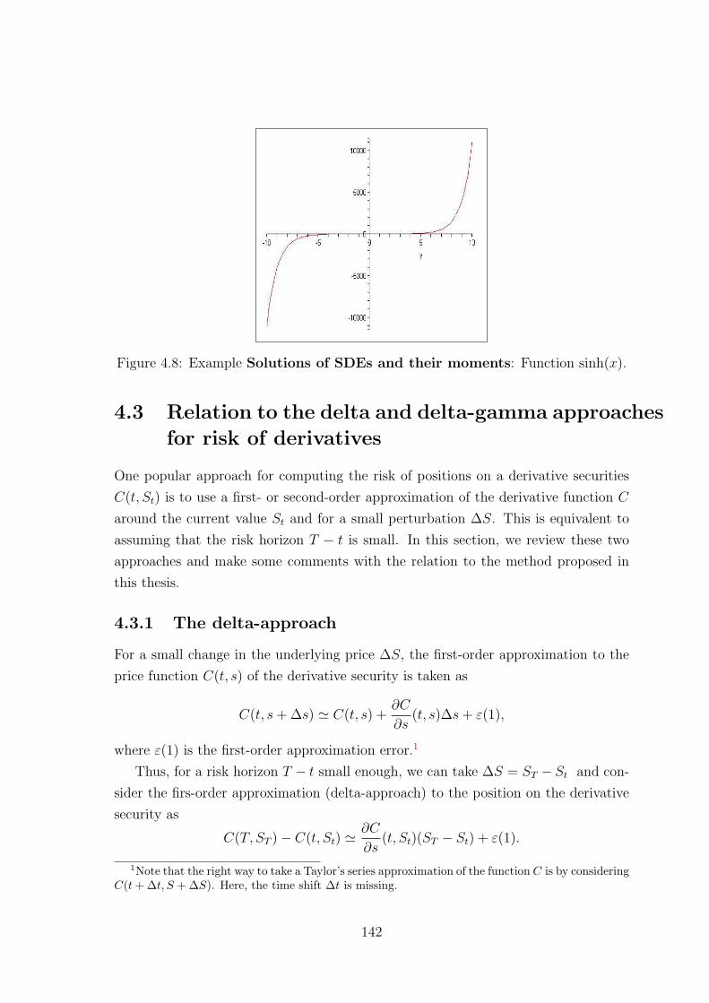
Figure 4.8: Example Solutions of SDEs and their moments: Function sinh(x).
4.3 Relation to the delta and delta-gamma approaches
for risk of derivatives
One popular approach for computing the risk of positions on a derivative securities
C(t, St) is to use a first- or second-order approximation of the derivative function C
around the current value St and for a small perturbation ∆S. This is equivalent to
assuming that the risk horizon T − t is small. In this section, we review these two
approaches and make some comments with the relation to the method proposed in
this thesis.
4.3.1 The delta-approach
For a small change in the underlying price ∆S, the first-order approximation to the
price function C(t, s) of the derivative security is taken as
C(t, s+ ∆s) ' C(t, s) +∂C
∂s(t, s)∆s+ ε(1),
where ε(1) is the first-order approximation error.1
Thus, for a risk horizon T − t small enough, we can take ∆S = ST − St and con-
sider the firs-order approximation (delta-approach) to the position on the derivative
security as
C(T, ST )− C(t, St) '∂C
∂s(t, St)(ST − St) + ε(1).
1Note that the right way to take a Taylor’s series approximation of the function C is by consideringC(t + ∆t, S + ∆S). Here, the time shift ∆t is missing.
142
If in addition, we can assume that the factor ∂C∂s
(t, St) stays constant on [t, T ],
then the risk of the position on the derivative security can be approximate as the risk
of a linear function on the position on the underlying asset St, this is
ρ(C(T, ST )− C(t, St)) '∂C
∂s(t, St)ρ (ST − St) .
This is of course an easier problem to solve than the original one. As an example,
consider as the risk measure ρ the VaR, and as the derivative security a European
call option C(t, St). Then
VaRα(C(T, ST )− C(t, St)) '∂C
∂s(t, St)VaRα (ST − St) .
This is, the delta-approximation to the VaR of a position on a call option is equal to
the VaR of the underlying position ST − St times the delta of the call option.
4.3.2 The delta-gamma approach
When the first-order approximation of a derivative is not sufficient accurate, a second-
order approximation may help.
For a small change in the underlying price ∆S, the second-order approximation
to the price function C(t, s) of the derivative security is taken as
C(t, s+ ∆s) ' C(t, s) +∂C
∂s(t, s)∆s+
1
2
∂2C
∂s2(t, s) (∆s)2 + ε(2),
where ε(2) is the second-order approximation error and assumed to be smaller, for
sufficient small s, than the first-order error ε(1).
Thus, for a risk horizon T − t small enough, we can take ∆S = ST − St and
consider the second-order approximation (gamma-approach) to the position on the
derivative security as
C(T, ST )− C(t, St) '∂C
∂s(t, s)(ST − St) +
1
2
∂2C
∂s2(t, s) (ST − St)
2 .
In this case, we need to assume that the terms ∂C∂s
(t, St) and ∂2C∂s2 (t, St) stay constant
on [t, T ]. Thus the risk of the position on the derivative security C is approximated
as the risk of a quadratic function on the position on the underlying asset St, this is
ρ(C(T, ST )− C(t, St)) ' ρ
(∂C
∂s(t, s)(ST − St) +
1
2
∂2C
∂s2(t, s)(ST − St)
2
).
One of the main drawbacks of the delta- and delta-gamma-approaches is the as-
sumption that the movement in the underlying asset price is small (or equivalently
143
small risk horizon T − t), and therefore the approximation may not be very accurate.
Specially in the situation where the price function of the derivative security is far from
linear or quadratic. The method presented in this chapter does not require to make
the assumption of a small risk horizon T − t. But instead, it requires to solve a final
value PDE, which, apart from few cases on the dynamics of the underlying process
St and option prices functions C(t, St), the PDE will not have explicit solution. In
such a case, series expansion solutions or accurate numerical methods may be applied.
Another alternative is to use Monte Carlo simulation, but this usually requires large
computational capacity.
4.4 Risk measures for American derivatives
In the situation when the derivative security for which one needs to measure the risk
is of American type, we can also formulate the the value of the risk measure (WCS,
VaR and AVaR) as the solution of a PDE, but in this case, the system to solve will
be a free-boundary problem with a final condition.
144
Chapter 5
Hedging and Derivative Pricing inthe Robust ε-expected ShortfallProblem
5.1 Introduction
In this chapter, we analyse a variant of the robust version of the expected shortfall
hedging problem:
For an initial capital x ≥ 0, find a hedging strategy (x, π), π ∈ A(x) with terminal
value X(x,π)T such that
infπ∈A(x)
supQ∈P
EQ
[(HT −X
(x,π)T
)+], (5.1)
in a continuous-time model consisting of two risky assets St and Yt, 0 ≤ t ≤ T (given
by Ito diffusions) and a risk-free bond Bt, 0 ≤ t ≤ T . The asset St is assumed to be
traded in the financial market but not Yt.
We consider a random payoff HT to be a function of the underlying process Yt at
time T , this is HT = H(YT ) and the set of measures (priors) P to be a subset all
equivalent probability measures Me.
The problem in (5.1) corresponds to the hedging problem for the WCSP risk
measure discussed in Chapter 1, Section 1.5.1.1. For the particular choice of priors
P = P and P = Q ∈Ma : dQdP is P ≤ 1
α defined in Proposition 30, we recover the
solution to the hedging problems corresponding to VaRα and AVaRα, respectively.
In view of the fact that the theory for the primal-dual formulation to the robust
versions of expected utility problems has only been recently developed in [82] and
under the assumptions that the utility function is a strictly increasing and strictly
145
concave function, we reformulate our original problem in (5.1) to fit with these as-
sumptions by considering an ε-approximation of the shortfall utility function (x)+ for
0 ≤ ε ≤ 1 by considering the following problem:
infπ∈A(x)
supQ∈P
EQ
[Uε
(H(YT )−X
(x,π)T
)]. (5.2)
with
Uε(x) = ε log
(1 + exp
−x
ε
exp
−x
ε
).
This is, when ε −→ 0 we recover the original expected shortfall problem.
Due to the fact that the utility function Uε(x) is not separable in its variables, we
are not able to solve explicitly in (5.2), but instead, we use a power series approxi-
mation in the dual variables. It turns out that the approximate solution to (5.2) is
the solution to the corresponding robust version of a utility maximisation problem
with exponential preferences (U(x) = − 1γe−γx) for a preferences parameter γ = 1
ε.
Then the original expected shortfall problem recovered when ε −→ 0 will correspond
to γ → ∞. For the approximate problem, we analyse the cases with and without
random endowment, and obtain an expression for the utility indifference bid price
corresponding to the liability HT = H(YT ).
5.2 The financial model
We consider an investment model of a single agent who manages her portfolio by
investing in a bond and a risky asset St which is tradable in the market and we also
consider a risky non-tradable asset Yt.
The bond price Bt is given by
dBt = rBtdt, B0 = B (5.3)
where r ≥ 0 is the interest rate. The tradable risky asset is modelled as a diffusion
process St solving
dSt = µStdt + σStdWst (5.4)
with S0 = s0 > 0. The non-tradable risky process, which can be conceived as an
“stochastic factor” is assumed to satisfy
dYt = bYtdt + aYtdWyt (5.5)
for Y0 = y and µ, b, σ and a constants. The processes W st and W y
t are Brownian
motions correlated with correlation coefficient ρsy ∈ [−1, 1].
146
The assumption of geometric Brownian motions for the dynamics for St and Yt
is basically to be able to have some explicit solutions, but this assumption can be
relaxed.
It is convenient to express W y as a linear combination of two independent Brow-
nian motions W and W s. Thus if
W yt = ρsyW
st + ρsyWt
for ρsy =√
1− ρ2sy the dynamics of Y remains
dYt = bYtdt + ρsyaYtdWst + ρsyaYtdWt
Remark 102 Note that by the specific shape of the coefficients in the process St, the
process Yt does not depend on St. This assumption simplifies the computations.
When |ρsy| < 1 we are in an incomplete market situation as the agent cannot
trade in Y . If ρsy = 1 then we are in the complete market case and the coefficients
in the SDEs for St and Yt must be related as follows:1
b = r +a
σ(µ− r) .
5.3 The wealth process
The investor starts at time t, with an initial capital x and re-balances her portfolio
holdings by dynamically choosing at any time s ∈ [t, T ] and 0 ≤ t ≤ T , the amounts
(money) Π0s and Πs to be invested, respectively, in the bond and the risky asset S.
Her total wealth process Xt satisfies the budget constraint
Xs = Π0s + Πs
and using the dynamics in (5.3) and (5.4) of the bond B and the risky asset St, the
current wealth Xs satisfies the following controlled diffusion equation:
dXu = rXudu + (µ− r)πuXudu + σπuXudWsu . (5.6)
with initial value Xt = x ≥ 0, 0 ≤ t ≤ T (see [51, Ch. 5.8] for more detail on this).
The quantity πt = Πt/Xt represents the proportion of wealth invested in the risky
asset.
In order to avoid arbitrage opportunities, the wealth process must also satisfy the
usual state constraint,
Xu ≥ 0 a.s. t ≤ u ≤ T. (5.7)
1The Sharpe ratios of the discounted price processes need to be equal to avoid arbitrage oppor-tunities.
147
Assumption 103 We assume the investor does not have the opportunity to consume
part of her wealth nor to introduce any exogenous funds during the trading interval
[t, T ].
Apart from condition (5.7), a process πs is considered to be admissible if it is Fs-
progressively measurable and satisfies the integrability condition E[∫ T
tπ2
sds]< ∞
a.s. The set of admissible controls (or policies) given the initial capital x will be
denoted by A(x).
5.4 Equivalent measures
Let us denote by Me the set of measures equivalent2 to P, and by PMb the set of
progressively measurable process ϕt such that∫ T
0ϕ2
tdt <∞ P-a.s.
If Q is a probability measure equivalent to P on FT then there exists a vector
process ϕt = (ϕ1t, ϕ2t) whose components ϕ1t, ϕ2t ∈ PMb, 0 ≤ t ≤ T (called Girsanov
kernels) are such that
dQdP|Ft = Dϕ
t := exp
(∫ t
0
ϕ1τdWsτ −
1
2
∫ t
0
ϕ21τdτ +
∫ t
0
ϕ2τdWτ −1
2
∫ t
0
ϕ22τdτ
).
(5.8)
Under the measure Q the processes W st and Wt defined by
W st = W s
t −∫ t
0
ϕ1τdτ
Wt = Wt −∫ t
0
ϕ2τdτ
are independent Q- Brownian motions.
5.4.1 Local martingale measures
As St is the only traded asset, a measure Q given in (5.8) will be a risk-neutral
measure if the discounted process e−rtSt is a Q-local martingale, but this is true if
and only if
ϕ1t = −% with % :=µ− r
σ.
The quantity % is called the “market price of risk”.
In this case, the set Me is in one-to-one correspondence with the set of integrands
ϕ2t in (5.8).
2Whenever a measure Q is equivalent to P will be denoted by Q ∼ P.
148
Then under a risk-neutral measure Q the dynamics of our processes St and Yt
satisfy
dSt = rStdt + σStdWs
t
dYt = Yt [b− ρsya%+ ρsyaϕ2t] dt + aYtdWy
t
where W yt = ρsyW
st + ρsyWt is a Brownian motion under Q. From the expression of
the dynamics of Yt under Q, we see that Yt can have arbitrary drift.
5.4.2 The minimal martingale measure
Denote by Q0 the risk-neutral measure corresponding to the special case in (5.8) when
ϕ2t = 0. Its Radon-Nikodym derivative remains
dQ0
dP|Ft = exp
(−∫ t
0
%dWsτ −
1
2
∫ t
0
%2dτ
). (5.9)
The measure Q0 is called the minimal martingale measure, and it is the measure,
that apart from making the discounted price process for the traded asset S a local-
martingale, leaves unaffected the Brownian motion W .
5.5 The set of priors P
Note that for a given hedging strategy (x, π), π ∈ A(x), x ≥ 0 the inner part of the
robust hedging problem in (5.1),
supQ∈P
EQ
[(HT −X
(x,π)T
)+],
is nothing else than computing WCS on a position(HT −X
(x,π)T
)+
. Thus, similarly
as in Section 3.3.5, this problem can be seen as a stochastic control problem, but here
on two controls κ1t and κ2t, the Girsanov kernels (or equivalently the control variable
is a two-dimensional vector κt). Based on similar arguments as in Section 3.3.5, in
order to be able to formulate the problem as a solution of a PDE, we need to restrict
the controls to a compact set. Therefore our class of priors will be given by3
P :=
Q ∼ P
∣∣∣∣∣∣dQdP = Dκ
t as in (5.8), κ = (κ1, κ2) ∈ K,K ⊂R2 fixed compact convex set
and κ1, κ2 ∈ PMb
. (5.10)
For simplicity in the notation, we make the following assumption.
3PMb is the set of progressively measurable process ϕt such that∫ T
0ϕ2
t dt < ∞ P-a.s.
149
Assumption 104 Assume r = 0, or equivalently, that the dynamics of St, Yt and
Xt are in discounted terms.
5.6 The robust ε-expected shortfall hedging prob-
lem
In this section, we return to our problem in (5.1), the robust version of the expected
shortfall hedging problem, and give the basis for the reformulation as a usual utility
maximisation problem with robust preferences.
Assume the investor needs to pay the random amount H(YT ) at time T for H a
continuous positive function. For a hedging strategy (x, π), π ∈ A(x) that define a
final value wealth XT at time T as in (5.6) and a set of prior models as in (5.10), the
robust version of the expected shortfall hedging problem is
infπ∈A(x)
supQ∈P
EQ
[(H(YT )−X
(x,π)T
)+].
One first step to the reformulation of the problem is to highlight the dependence
on the state of the utility function. This is, for each H(YT ) define the state-dependent
function UH,ω(x) = (H(YT )(ω)− x)+, and write the problem (5.1) as4
infπ∈A(x)
supQ∈P
EQ
[UH
(X
(x,π)T
)].
When P = P (no robust preferences), convex duality methods for solving ex-
pected utility of final wealth problems have been widely used in the last decade (see
[52, Ch. 3 and 5]). It involves to solve the so-called primal and dual problems (see
Appendix B). In view that the theory for the primal-dual formulation to the robust
versions of expected utility problems has only been recently developed in [82] and
under the assumptions that the utility function is a strictly increasing and strictly
concave function, we consider a closely related problem to (5.1) in order to fit into
these assumption by considering an ε-approximation of the utility function UH,ω(x)
for 0 ≤ ε ≤ 1 by taking
UH,ωε (x) = ε log
1 + exp− (H(YT )(ω)−x)
ε
exp
− (H(YT )(ω)−x)
ε
.
In this way, the function UH,ωε (x) is strictly increasing and strictly convex in x.
4The function UH,ω(x) is increasing and convex in x but not strictly.
150
The reformulation of our problem for UH,ωε (x) into the usual maximisation of
expected utility of terminal wealth is analysed in the next section. Once reformulated
the problem, our aim is to use stochastic control techniques to solve the dual and
primal problems.
5.6.1 Reformulation of the problem
Define the function (see Figure 5.1(a))
Uε(x) = ε log
(1 + exp
−x
ε
exp
−x
ε
).
The robust ε-expected shortfall hedging problem is
infπ∈A(x)
supQ∈P
EQ
[Uε
(H(YT )−X
(x,π)T
)]. (5.11)
Define
UHε (x) = Uε(H(YT ))− Uε (H(YT )− x) . (5.12)
The function UHε (x) is strictly increasing and strictly concave in x (see Figure 5.1(b)).
The hedging problem in (5.11) is equivalent to the following problem:
supπ∈A(x)
infQ∈P
EQ
[UH
ε
(X
(x,π)T
)](5.13)
= supπ∈A(x)
infQ∈P
EQ
[Uε(H(YT ))− Uε
(H(YT )−X
(x,π)T
)]. (5.14)
The problem in (5.14) is the standard form of the problem treated in [82] (see Ap-
pendix B).
151
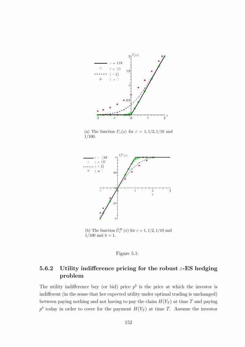
(a) The function Uε(x) for ε = 1, 1/2, 1/10 and1/100.
(b) The function UHε (x) for ε = 1, 1/2, 1/10 and
1/100 and h = 1.
Figure 5.1:
5.6.2 Utility indifference pricing for the robust ε-ES hedgingproblem
The utility indifference buy (or bid) price pb is the price at which the investor is
indifferent (in the sense that her expected utility under optimal trading is unchanged)
between paying nothing and not having to pay the claim H(YT ) at time T and paying
pb today in order to cover for the payment H(YT ) at time T . Assume the investor
152
has an initial wealth x′. Define
RH(x′) = supπ∈A(x′)
infQ∈P
EQ
[UH
ε
(X
(x′,π)T
)]where the supremum is taken over all wealths XT which can be generated from the
initial fortune x′. The utility indifference buy price pb is the solution to
RH(x′ − pb) = R0(x′).
Then, by solving the following two problems: 1) Maximising utility with no
random endowment
supπ∈A(x)
infQ∈P
EQ
[U0
ε
(X
(x,π)T
)](P1)
and 2) Maximising utility with a random endowment
supπ∈A(x)
infQ∈P
EQ
[UH
ε
(X
(x,π)T
)](P2)
for arbitrary initial capital x, we recover as a by-product the indifference bid price pb.
5.6.3 Maximising utility with no random endowment
Assume the current time is zero. When there is no random endowment (no claim to
be paid at time T ), by (5.12) the term U0ε
(X
(x,π)T
)in (P1) reduces to
Uε(0)− Uε
(−X(x,π)
T
).
Define Uε (x) by
Uε (x) := −Uε (−x) = −ε log
(1 + exp
xε
exp
xε
). (5.15)
The function Uε (x) is strictly increasing and strictly concave in x. The problem P1
is equivalent to
u(x) = supπ∈A(x)
infQ∈P
EQ
[Uε
(X
(x,π)T
)], (5.16)
plus a constant term of ε log 2.
The main idea to solve (5.16) is to look at it from the perspective of a usual
stochastic control problem with controls in a compact set. This can be accomplished
by showing that all assumptions in [82] (see Appendix B) for the equality to the
primal and dual problem are satisfied. The reformulation to the problem in (5.16)
153
as a usual stochastic control problem results from working with the dual problem
rather than with the primal problem itself. It turns out that the control variable
is given by a vector formed of a triplet of Girsanov kernels that define equivalent
probability measures to P on a compact set. This technique has already been used
to solve utility maximisation problems in [13] for an exponential utility function with
P =P and recently in the robust case in [43] for a power utility function and in [42]
for a logarithmic utility function with a penalty term.
In relation with utility maximisation problems including no traded assets but when
no robust preferences are considered [39], [60], and [58] have treated the problem using
exponential preferences. Also in incomplete markets, but in a stochastic volatility
framework, [49] works with the HJB equation and the dual formulation to solve a
problem of minimising expected shortfall.
We summarise the key results of the solution to the robust problem (5.16) in the
following theorem.
Theorem 105 Assume the current time is t, 0 ≤ t ≤ T . The value function u(t, x)
of the robust utility maximisation problem (5.16) can be approximated by
uapprox(t, x) = −ε exp−xε
exp
−1
2%2(T − t)
×
exp
−%Eκ2
[∫ T
t
κ1τdτ
]− 1
2Eκ2
[∫ T
t
κ21τdτ
],
with an error of
u(t, x)− uapprox(t, x) ≤ 1
2(1− log(2)) ε ≈ 0.1534264097ε.
Here κ = (κ1, κ2) ∈ K is a pair of Girsanov kernels that solve
min(κ1,κ2)∈K
Eκ2
[∫ T
t
(%+ κ1τ )2 dτ
].
The operator Eκ2 [·] represents the expected value under the measure Qκ2 given by
dQκ2
dP|FT
= Z κ2T := E
(−∫
0
%dWsτ +
∫0
κ2τdWτ
)T
.
The corresponding approximate optimal strategy πapprox for the robust problem is
Πapproxt = πapprox
t Xx,πt =
ε
σ(%+ κ1t) .
154
Define the measure Q ∈P via
dQdP|FT
= DκT := exp
(∫ T
0
κ1τdWsτ −
1
2
∫ t
0
κ21τdτ +
∫ t
0
κ2τdWτ −1
2
∫ t
0
κ22τdτ
).
Then the pair(πapprox
t , Q)
is a saddle point for the problem
uapprox(t, x) = supπ∈A(x)
infQ∈P
EQ
[Uε
(X
(x,π)T
)],
with Uε (x) = −ε exp−x
ε
.
The proof of the above theorem will be divided into several parts and developed
through this section.
Remark 106 The approximated value function uapprox(t, x) solves the robust utility
maximisation problem for exponential utility function. When P = P (no robust
preferences), we have (κ1t, κ2t) = (0, 0) and we recover the usual solution (see [13],
[60] and [39]).
One of the key elements to the solution to the robust problem (5.16) is the use of
the dual-primal relations and results developed in [82, Theorem 2.2] for robust utility
maximisation problems (see Appendix B).
Lemma 107 For the utility functions Uε(x) = −ε log
(1+expx
εexpx
ε
)and Uε(x) =
−ε exp−x
ε
, and the priors set P defined in (5.10), the assumptions in [82, Theorem
2.2] are satisfied.
Proof. See Section B.4 in Appendix B on page 189.
For simplicity in the notation, assume for this discussion that the current time is
t = 0 and omit the time dependence in the primal value function u, i.e., we write
only u(x).
For any ζ ∈ PM (progressively measurable process), define
Zζt := E
(∫0
−%dWsτ +
∫0
ζτdWτ
)t
. (5.17)
Given E[ZT ] = 1, each Zζt would correspond to a density process that defines an
equivalent probability measure to P.
155

By Lemma 107 and therefore using results in [82], the dual value function of the
robust utility maximisation problem is given by (see Appendix B on page 189)
v(λ) := infκ∈K
infζ∈PM
E
[Dκ
T Vε
(λZζ
T
DκT
)], λ > 0 (5.18)
where the the vector process κ and the set K are defined in (5.10), the parameter λ
plays the role of a Lagrange multiplier in the optimisation problem and the function
V (y) is the Legendre-Fenchel transform of Uε(x) and given by5
Vε(y) = supx≥0
(Uε(x)− yx
)=
∞ if y ≥ 1
−ε log(
11−y
)− εy log
(1−y
y
)if 0 < y < 1.
The primal and dual value functions are related as follows:
u(x) = minλ>0
(v(λ) + λx) .
Assume for each x > 0 the solution to the above minimisation problem is well defined
(it has a solution 0 < λmin(x) <∞, with∣∣v(λmin(x))
∣∣ <∞), then the value function
of the robust primal problem can be computed as
u(x) = v(λmin(x)) + λmin(x)x,
with λmin(x) satisfying the relation
dv
dλ(λmin(x)) = −x.
As the expression
Vε
(λZζ
T
DκT
)=
∞ if λ
ZζT
DκT≥ 1
−ε log
1
1−λZ
ζT
DκT
− ελZζ
T
DκT
log
1−λZ
ζT
DκT
λZ
ζT
DκT
if 0 < λZζ
T
DκT< 1,
in (5.18) is not separable of variables in λ, in the next section we find a series ap-
proximation in λ to λmin(x) and set conditions for the finiteness of the approximated
primal value function.
5The maximum as attained at
x∗ =
0 if z ≥ 1ε log
(1−z
z
)if 0 < z < 1.
156
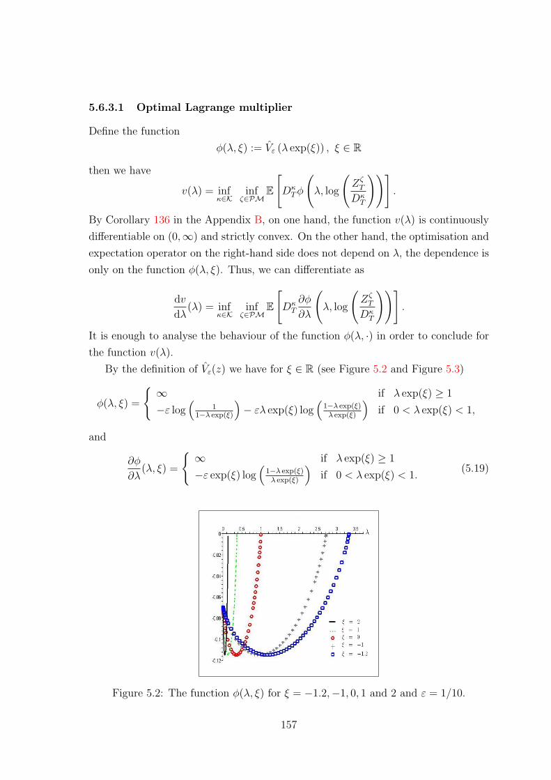
5.6.3.1 Optimal Lagrange multiplier
Define the function
φ(λ, ξ) := Vε (λ exp(ξ)) , ξ ∈ R
then we have
v(λ) = infκ∈K
infζ∈PM
E
[Dκ
Tφ
(λ, log
(Zζ
T
DκT
))].
By Corollary 136 in the Appendix B, on one hand, the function v(λ) is continuously
differentiable on (0,∞) and strictly convex. On the other hand, the optimisation and
expectation operator on the right-hand side does not depend on λ, the dependence is
only on the function φ(λ, ξ). Thus, we can differentiate as
dv
dλ(λ) = inf
κ∈Kinf
ζ∈PME
[Dκ
T
∂φ
∂λ
(λ, log
(Zζ
T
DκT
))].
It is enough to analyse the behaviour of the function φ(λ, ·) in order to conclude for
the function v(λ).
By the definition of Vε(z) we have for ξ ∈ R (see Figure 5.2 and Figure 5.3)
φ(λ, ξ) =
∞ if λ exp(ξ) ≥ 1
−ε log(
11−λ exp(ξ)
)− ελ exp(ξ) log
(1−λ exp(ξ)
λ exp(ξ)
)if 0 < λ exp(ξ) < 1,
and
∂φ
∂λ(λ, ξ) =
∞ if λ exp(ξ) ≥ 1
−ε exp(ξ) log(
1−λ exp(ξ)λ exp(ξ)
)if 0 < λ exp(ξ) < 1.
(5.19)
Figure 5.2: The function φ(λ, ξ) for ξ = −1.2,−1, 0, 1 and 2 and ε = 1/10.
157
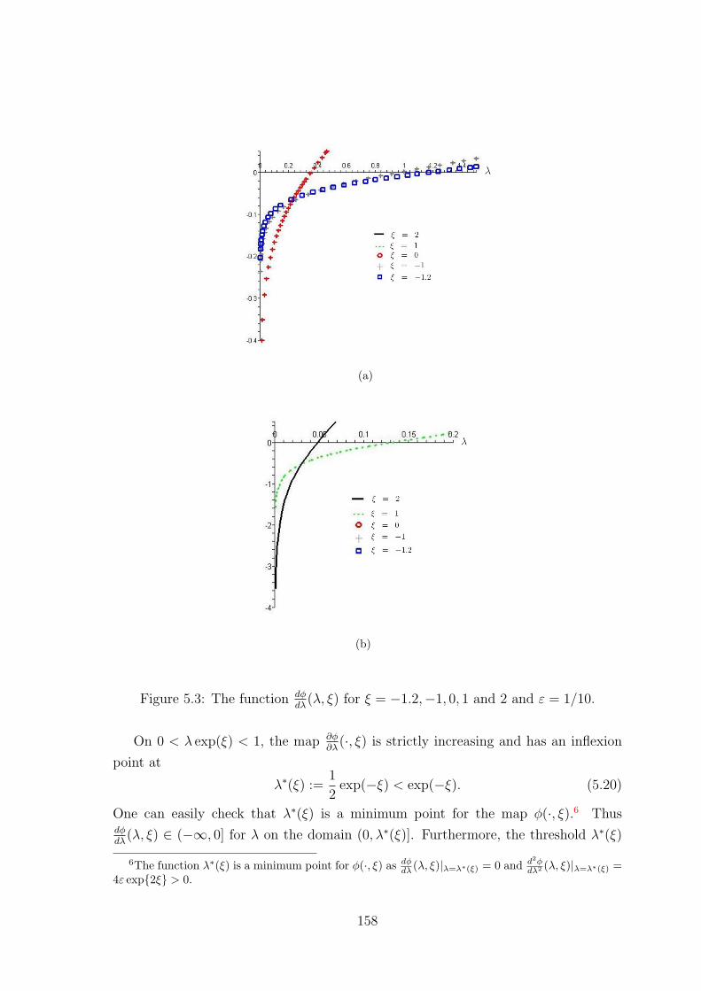
(a)
(b)
Figure 5.3: The function dφdλ
(λ, ξ) for ξ = −1.2,−1, 0, 1 and 2 and ε = 1/10.
On 0 < λ exp(ξ) < 1, the map ∂φ∂λ
(·, ξ) is strictly increasing and has an inflexion
point at
λ∗(ξ) :=1
2exp(−ξ) < exp(−ξ). (5.20)
One can easily check that λ∗(ξ) is a minimum point for the map φ(·, ξ).6 Thusdφdλ
(λ, ξ) ∈ (−∞, 0] for λ on the domain (0, λ∗(ξ)]. Furthermore, the threshold λ∗(ξ)
6The function λ∗(ξ) is a minimum point for φ(·, ξ) as dφdλ (λ, ξ)|λ=λ∗(ξ) = 0 and d2φ
dλ2 (λ, ξ)|λ=λ∗(ξ) =4ε exp2ξ > 0.
158

is decreasing in ξ ∈ R.Now, if we define
Ψκ,ζ(λ) = E
[Dκ
T
∂φ
∂λ
(λ, log
(Zζ
T
DκT
))],
and substituting from (5.19) we obtain
Ψκ,ζ(λ) = E
−εZζT
log
1− λ(
ZζT
DκT
)λ(
ZζT
DκT
) . (5.21)
The properties of ∂φ∂λ
(·, ξ) are inherited to the map Ψκ,ζ(·), this is, Ψκ,ζ(·) is strictly
increasing and has an inflexion point at
λ∗κ,ζ := E
[λ∗
(log
(Zζ
T
DκT
))]=
1
2E
[Dκ
T
ZζT
]< E
[Dκ
T
ZζT
].
Thus on (0, λ∗κ,ζ ], the function Ψκ,ζ(λ) ∈ (−∞, 0] is strictly convex and strictly in-
creasing. Moreover, Ψκ,ζ(λ) is related to the dual value function of the robust problem
asdv
dλ(λ) = inf
κ∈Kinf
ζ∈PMΨκ,ζ(λ).
Finally, by the properties of Ψκ,ζ(λ) and for each x ≥ 0 we can conclude that the
equation
infκ∈K
infζ∈PM
Ψκ,ζ(λ) = −x,
has a unique finite solution λmin(x) with 0 < λmin(x) < λ∗κ,ζ .
Let us now analyse how to compute λmin(x). One one hand, note that if∫ T
0ζtdt <
∞ then ZζT and log
(Dκ
T
ZζT
)will be bounded, which would imply that E
[Zζ
T
]= 1,
E[
DκT
ZζT
]= 1 and E
[log(
DκT
ZζT
)]< ∞. On the other hand, by the shape of Ψκ,ζ in
(5.21) we cannot find directly an explicit expression for λmin(x). Thus if∫ T
0ζtdt <∞,
then
0 < λmin(x) < λ∗κ,ζ < E
[Dκ
T
ZζT
]= 1,
and as the function inside the expectation operator in (5.21) is of logarithmic type,
then we could use a series expansion approximation on λ on the region (0,∞). This
is, using
log
(1− λz
λz
)≈ − log(z)− log(λ) +O(λ),
159
we have
Ψκ,ζ(λ) ≈ E
[−εZζ
T
− log
(Zζ
T
DκT
)− log (λ)
]
= εE
[Zζ
T log
(Zζ
T
DκT
)]+ ε log(λ)E
[Zζ
T
]= εEζ
[log
(Zζ
T
DκT
)]+ ε log(λ)E
[Zζ
T
].
In such a case, the function λmin(x) can be approximated by
λmin(x) ≈ λmin approx(x) := exp−xε
exp
− inf
κ∈Kinf
ζ∈PMΛκ,ζ
, (5.22)
with
Λκ,ζ := Eζ
[log
(Zζ
T
DκT
)]. (5.23)
The following lemma supports the assumption that it is enough to take processes
ζt with∫ T
0ζ2t dt bounded.
Define
PMb :=
ζ ∈ PM :
∫ T
0
ζ2t dt is P-a.s. bounded
.
Lemma 108 For fixed κ ∈ K we have
infζ∈PM
Λκ,ζ = infζ∈PMb
Λκ,ζ .
Proof. Firstly, note that for ζ ∈ PM, and under the measure Qζ given by dQζ
dP |Ft =
Zζt , and Zζ
t defined in (5.17) and using Dκt given as in (5.8) the random variable
ZζT
DκT
has the form
ZζT
DκT
= exp
−∫ T
0(%+ κ1τ ) dW
s
τ + 12
∫ T
0(%+ κ1τ )
2 dτ+∫ T
0(ζτ − κ2τ ) dWτ + 1
2
∫ T
0(ζτ − κ2τ )
2 dτ
,
with W st and Wt two Qζ-Brownian motions given by
W st = W s
t +
∫ t
0
%dτ
Wt = Wt −∫ t
0
ζτdτ.
160
Thus,
Λκ,ζ : = Eζ
[log
(Zζ
T
DκT
)]
= Eζ
[1
2
∫ T
0
(%+ κ1τ )2 dτ +
1
2
∫ T
0
(ζτ − κ2τ )2 dτ
].
By the expression of Λκ,ζ we have for any κ2 ∈ PMb and any ζ ∈ PM either
0 < Λκ,κ2 = Λκ,κ2 · 1κ2∈PMb ≤ Λκ,ζ ≤ Λκ,0,
or
0 < Λκ,κ2Λκ,κ2 · 1κ2∈PMb ≤ Λκ,0 ≤ Λκ,ζ .
Then
0 ≤ infκ2∈PMb
Λκ,κ2 ≤ infζ∈PM
Λκ,ζ .
On the other hand, as PMb ⊆ PM we have
infζ∈PM
Λκ,ζ ≤ infκ2∈PMb
Λκ,κ2 ≤ Λκ,0.
Putting this both conditions together we obtain
0 ≤ infζ∈PM
Λκ,ζ = infκ2∈PMb
Λκ,κ2 ≤ Λκ,0.
5.6.3.2 An approximation to the dual and primal value functions
In this section, we compute approximations to the primal value function u(x) and the
dual value function v(λ) using a similar series expansion as in previous section.
Define
φapprox (λ, ξ) := −ελ expξ (1− ξ − log(λ)) , (5.24)
then the series expansion for φ (λ, ξ) is given by
φ (λ, ξ) ≈ φapprox (λ, ξ) +O(λ2).
The approximation error between the function φ (λ, ξ) and the series expansion
approximation φapprox (λ, ξ) only depends on ε, as it is stated in the following lemma.
This property is important as one may use ε as a parameter to control the error and
get the desired accuracy.
161
Lemma 109 For any ξ ∈ R, any 0 < λ < λ∗(ξ) and ε ≥ 0, the maps φ (·, ξ) and
φapprox (·, ξ) are strictly decreasing and strictly convex. Furthermore,
0 ≤ φ (λ, ξ)−φapprox (λ, ξ) ≤ φ (λ∗(ξ), ξ)−φapprox (λ∗(ξ), ξ) =1
2(1− log(2)) ε ≈ 0.1534264097ε.
Proof. The fact that the function φ (·, ξ) is strictly decreasing and strictly convex
follows from the properties of the function Vε (z). That φapprox (·, ξ) satisfies similar
properties can be directly checked by its definition.
In order to prove the inequalities, note that limλ↓0+ φ (λ, ξ) = limλ↓0+ φapprox (λ, ξ) =
−ε log(2). The function φ (·, ξ) attains its minimum at λ∗(ξ) = 12exp(−ξ) and the
function φapprox (·, ξ) at λapprox(ξ) = e exp(−ξ). But λ∗(ξ) < λapprox(ξ) for any ξ ∈ R.
On the other hand, for any ξ ∈ R, any 0 < λ < λ∗(ξ) and ε ≥ 0 we have
∂φapprox
∂λ(λ, ξ) ≤ ∂φ
∂λ(λ, ξ) ,
which proves the left-hand side of the inequality. This also suggests that the maximum
gap between the functions is reached at λ∗(ξ). Direct substitution of λ∗(ξ) in φ (λ, ξ)
and φapprox (λ, ξ) show that the difference φ (λ, ξ)− φapprox (λ, ξ) does not depend on
ξ nor on λ for 0 < λ < λ∗(ξ). This concludes the proof.
Recall that the dual value function v(λ) to the robust problem is given by
v(λ) = infκ∈K
infζ∈PMb
E
[Dκ
Tφ
(λ, log
(Zζ
T
DκT
))].
We use the series expansion of φ (λ, ξ) to approximate the term inside the expectation
operator in v(λ) as follows.
E
[Dκ
Tφ
(λ, log
(Zζ
T
DκT
))]≈ E
[Dκ
Tφapprox
(λ, log
(Zζ
T
DκT
))]
= E
[−ελZζ
T
(1− log
(Zζ
T
DκT
)− log(λ)
)]= −ελ (1− log(λ)) + ελΛκ,ζ ,
with Λκ,ζ as defined in (5.23). Then the approximation to the dual value function
v(λ) is
v(λ) ≈ −ελ (1− log(λ)) + ελ
infκ∈K
infζ∈PMb
Λκ,ζ
=: vapprox(λ). (5.25)
162
We can now use the above approximation evaluated at λmin approx(x) to obtain an
expression for the approximation to the primal value function u(x) to the robust
problem. This is,
uapprox(x) = −ε exp−xε
exp
− inf
κ∈Kinf
ζ∈PMb
Λκ,ζ
. (5.26)
5.6.3.3 The solution to the dual problem
In this section, we obtain the solution to
infκ∈K
infζ∈PMb
Λκ,ζ . (5.27)
In order to capture the dynamical behaviour of the problem, assume now the
starting time is t ∈ [0, T ].
Using the definition of Λκ,ζ in (5.23), take
Jκ,ζt : = Eζ
[log
(Zζ
T
DκT
)]
= Eζ
[1
2
∫ T
t
(%+ κ1τ )2 dτ +
1
2
∫ T
t
(ζτ − κ2τ )2 dτ
].
The problem is to find processes (κ, ζ) ∈ K × PMb that solves
infκ∈K
infζ∈PMb
Jκ,ζt . (5.28)
Assume (κ, ζ) is optimal in (5.28), then we recover the solution to (5.27) as Λκ,ζ =
J κ,ζ0 . And the approximated value function uapprox(x) to the primal problem in (5.16)
for utility maximisation with zero random endowment is given by
uapprox(x) = −ε exp−xε
exp
−J κ,ζ
0
.
Note that the dual problem in (5.28) does not depend on any of the dynamics St, Yt
nor Xt, and the solution can be easily characterised as in the following proposition.
Proposition 110 There exists (κ, ζ) ∈ K × PMb, which attains the minimum for
the dual problem (5.28). Furthermore, such a pair (κ, ζ) is characterised by the fact
that κ1t and κ2t solves
Eκ2
[∫ T
t
(%+ κ1τ )2dτ
]= inf
(κ1,κ2)∈KEκ2
[∫ T
t
(%+ κ1τ )2dτ
], (5.29)
163
and ζt = κ2t. Thus the value function to the dual problem in (5.28) is given by
J κ,ζt =
1
2Eκ2
[∫ T
t
(%+ κ1τ )2 dτ
]=
1
2%2(T − t) + %Eκ2
[∫ T
t
κ1τdτ
]+
1
2Eκ2
[∫ T
t
κ21τdτ
].
Proof. By the compactness of the set K and as ζ ∈ PMb, the existence of (κ, ζ) ∈K × PMb is guaranteed. And by Lemma 108 (see proof) we know that Λκ,ζ ≥ Λκ,κ2
for all (κ1, κ2) ∈ K and any ζ ∈ PMb. Then the original problem in (5.28) is reduced
to
inf(κ1,κ2)∈K
Eκ2
[∫ T
t
(%+ κ1τ )2dτ
].
This proves the characterisation to the optimal solution.
Remark 111 Define the measures Q by
dQdP|FT
= DκT .
In the case the set K is a rectangle with deterministic edges of the form [k−1 , k+1 ]×
[k−2 , k+2 ], k−1 , k
+1 , k
−2 , k
+2 ∈ R, the optimal Girsanov kernels are
κ1 =
κ+
1 if κ+1 < −%
−% if κ−1 ≤ −% ≤ κ+1
κ−1 if κ−1 > −%
and κ2 is any κ2 ∈ PMb with (κ1, κ2) ∈ K and ζ1 = κ2. The dual value function in
(5.28) is given by
J κ,ζt =
1
2(%+ κ1)
2 (T − t).
Remark 112 When P = P (no robust preferences), we have (κ1t ,κ2t) = (0, 0) or
equivalently dQκ
dP = 1 P-a.s. then for dQζ
dP = ZζT , Qζ ∈ Me defined as in (5.17) we
obtain
Λ0,ζ = Eζ
[log
(Zζ
T
D0T
)]
= E[dQζ
dPlog
(dQζ
dP
)]= H(Qζ |P).
where
H(Q|P) : =
E[
dQdP log
(dQdP
)], if Q P on FT
+∞ otherwise.
164
The problem
infζ∈PMb
Λ0,ζ (5.30)
reduces to finding the minimal entropy martingale measure QE defined by
QE := arg minQ∈Me
H(Q|P).
But in our present setting with constant coefficients geometric Brownian motion pro-
cesses for St and Yt, the minimal entropy martingale measure QE and the minimal
martingale measure Q0 in (5.9) are the same, i.e., QE = Q0 (see [36]), then the
optimal ζ in (5.30) is given by ζ = −%.
5.6.3.4 Approximation to the optimal strategy
By [82, Theorem 2.6], the process Mt := Z ζtX
x,πt is a P-martingale. Hence as ζ = κ2
P-a.s and using the dynamics of Xx,πt in (5.6) and Z ζ
t in (5.17), we get
dMt = Z ζt dX
x,πt +Xx,π
t dZ ζt + d < Xx,π
t , Z ζ >t (5.31)
= Z ζtX
x,πt (µπtdt+ σπtdW
st ) +Xx,π
t Z ζt
(−%dW s
t + ζτdWt
)− Z ζ
tXx,πt %σπtdt
= Mt (σπt − %) dW st + κ2τdWt .
On the other hand, for the optimal control processes (κ, ζ) ∈ K × PMb by [82,
Theorem 2.6] there exists an optimal strategy π ∈ A(x), whose terminal wealth is
given by
Xx,πT = I
(λminZ ζ
T
DκT
),
where
I(y) = −V ′ε (y)
= ε
log
(1− y
y
).
Using again a series expansion in λ for
I(λz) = ε log
(1− λz
λz
)≈ −ε log(z)− ε log(λ) =: Iapprox(λz),
165
and evaluating at λmin approx(x) = exp−xε exp
−Λκ,ζ
, we have
I
(λminZ ζ
T
DκT
)≈ Iapprox
(λmin approxZ ζ
T
DκT
)
= −ε
log
(Z ζ
T
DκT
)+ log(λmin approx)
= −ε log
(Z ζ
T
DκT
)+ x+ εΛκ,ζ
= x− ε
log
(Z ζ
T
DκT
)− Λκ,ζ
.
Recalling thatZ ζ
T
DκT
under P is given by
Z ζT
DκT
|FT = exp
−∫ T
0
(%+ κ1τ ) dWsτ −
1
2
∫ T
0
(%2 − κ2
1τ
)dτ
,
and Λκ,ζ = 12Eκ2
[∫ T
0(%+ κ1τ )
2 dτ]
we obtain
Xx,πT = x− ε
−∫ T
0(%+ κ1τ ) dWs
τ − 12
∫ T
0(%2 − κ2
1τ ) dτ
−12Eκ2
[∫ T
0(%+ κ1τ )
2 dτ]
. (5.32)
Using again the fact that Mt := Z ζtX
x,πt is a P-martingale (i.e., Mt = E [MT |Ft] =
E[Z ζ
TXx,πT |Ft
]), but this time computing with the expression in (5.32) we obtain
Mt = Z ζt x−εZ
ζt
−∫ T
t
(%+ κ1τ ) dWsτ −
1
2
∫ T
t
(%2 − κ2
1τ
)dτ − 1
2Eκ2
[∫ T
0
(%+ κ1τ )2 dτ
]and after omitting the finite variation terms, we have
dMt = εZ ζtX
x,πt
(%+ κ1τ )
Xx,πt
dWsτ + Z ζ
tXx,πt −%dWs
τ + κ2τdWτ ,
or
dMt = Mt
(ε(%+ κ1t)
Xx,πt
− %
)dWs
t +Mtκ2tdWt.
Comparing here and in (5.31) all terms involving dW st yields
Πt = πtXx,πt =
ε
σ(%+ κ1t) .
166
5.6.4 Maximising utility with random endowment
When there is a random endowment to be paid at time T given by a claim H(YT ) on
the nontraded asset Yt the robust utility maximisation problem in (P2) is
uH(x) = supπ∈A(x)
infQ∈P
EQ
[UH
ε
(X
(x,π)T
)]. (5.33)
Recalling that
UHε (x) = Uε(H(YT ))− Uε (H(YT )− x)
and
Uε (x) := −Uε (−x) = −ε log
(1 + exp
xε
exp
xε
),
then adapting Lemma 143 in Appendix B to our present situation, the problem P2
is an upper bound for the problems (P2a) and (P2b) defined below. This is,
uH(x) ≥ −supQ∈P
EQ
[Uε (−H(YT ))
]︸ ︷︷ ︸
(P2a)
+ supπ∈A(x)
infQ∈P
EQ
[Uε
(X
(x,π)T −H(YT )
)]︸ ︷︷ ︸
(P2b)
. (5.34)
By Lemma 144, the equality in (5.34) will be satisfied provided each of the prob-
lems (P2a) and (P2b) attains the infimum at the same measure Q∗ ∈ P . Therefore
we make the following assumption.
Assumption 113 The set P and the payoff function H(y) are such that the optimal
measure Q∗ ∈ P in both problems (P2a) and (P2b) is the same, this is, there exist
Q∗ ∈ P such that
EQ∗
[Uε (−H(YT ))
]= sup
Q∈PEQ
[Uε (−H(YT ))
]and
supπ∈A(x)
EQ∗
[Uε
(X
(x,π)T −H(YT )
)]= sup
π∈A(x)
infQ∈P
EQ
[Uε
(X
(x,π)T −H(YT )
)]This assumption is useful as each of the two problems (P2a) and (P2b) above are
simpler to solve than the original problem in (5.33). We proceed by solving them
separately. But by the shape of the utility function Uε(x), an explicit solution is not
easy, instead, we use a series approximation to find upper bounds for the solution of
(P2a) and (P2b).
167

Remark 114 Assumption 113 is satisfied at least when no robust preferences are
present, or when the optimal pair of Girsanov kernels is (0, 0). Further investigation
on the conditions on K and H(y) that satisfy Assumption 113 is left for further
research.
We summarise the key results in the solution to the robust problem (5.33) in the
following theorem.
Theorem 115 Assume the current time is t, 0 ≤ t ≤ T , Yt = y and Xt = x, and
that Assumptions 113 and 116 hold. The value function uH(t, x) of the robust utility
maximisation problem (5.33) can be approximated by
uH approx(t, x) = −ua(t, y)− ε exp−xε
exp
−1
2%2(T − t) +
1
εh(t, y)
× exp
−%Eκ2
[∫ T
t
κ1τdτ
]− 1
2Eκ2
[∫ T
t
κ21τdτ
],
with an error of
uH(t, x)− uH approx(t, x) ≤ 1
2(1− log(2)) ε ≈ 0.1534264097ε.
And κ = (κ1, κ2) ∈ K is a pair of Girsanov kernels that solve
min(κ1,κ2)∈K
Eκ2
[1
2
∫ T
t
(%+ κ1τ )2 dτ − 1
εH(YT )
].
The operator Eκ2 [·] represents the expected value under the measure
dQκ2
dP|FT
= Z κ2T := E
(−∫
0
%dWsτ +
∫0
κ2τdWτ
)T
.
The function ua(t, y) is the solution to the following PDE
uat +
1
2a2y2ua
yy + byuay + sup
(κ1,κ2)∈K
(ρsyκ1 + ρsyκ2) ayu
ay
= 0,
with terminal condition
ua(T, y) = Uε (−H(y)) = −ε log
1 + exp−H(y)
ε
exp
−H(y)
ε
.
And the function h(t, y) solves
ht +1
2a2y2hyy + (b− ρsya%) yhy + inf
(κ1,κ2)∈Kρsyaκ2yhy = 0,
168
with terminal condition
h(T, y) = H(YT ).
The corresponding approximate optimal strategy πapproxt for the robust problem is
Πapproxt = πapprox
t Xx,πt =
ε
σ(%+ κ1t) + ρsy
a
σYtfy(t, Yt),
with f(t, y) given by
f(t, y) = exp
−1
2
b2
a2(T − t)
E[exp
b
a
√T − tN
H(y expa
√T − tN
)].
Define the measure Q ∈P via
dQdP|FT
= DκT := exp
(∫ T
0
κ1τdWsτ −
1
2
∫ t
0
κ21τdτ +
∫ t
0
κ2τdWτ −1
2
∫ t
0
κ22τdτ
).
Then the pair(πapprox
t , Q)
is a saddle point for the problem
uapprox(t, x) = supπ∈A(x)
infQ∈P
EQ
[Uε
(X
(x,π)T −H(YT )
)],
with Uε (x) = −ε exp−x
ε
.
5.6.4.1 The problem (P2b)
We analyse first the solution to the problem (P2b) above. This is the random endow-
ment counterpart of the problem solved in Section 5.6.3. We use the same technique
of solving first the dual problem and express the primal value function in terms of
the dual value function.
By Lemma 107 and therefore using results in [82], the dual value function of
the robust utility maximisation with random endowment problem is given by (see
Appendix B)
vb(λ) := infκ∈K
infζ∈PM
E
[Dκ
T Vε
(λZζ
T
DκT
)]− λE
[Zζ
TH(YT )]
, λ > 0 (5.35)
where the vector process κ and the set K are defined in (5.10), the parameter λ plays
the role of a Lagrange multiplier in the optimisation problem and the function V (y)
is the Legendre-Fenchel transform of Uε(x) and given by
Vε(y) = supx≥0
(Uε(x)− yx
)=
∞ if y ≥ 1
−ε log(
11−y
)− εy log
(1−y
y
)if 0 < y < 1.
169
The primal and dual value functions are related as follows:
ub(x) = minλ>0
(vb(λ) + λx
).
We use the same idea as in Section 5.6.3 of approximating the dual value function
vb(λ) by a series expansion in λ. This is, we use the approximation of Vε
(λ
ZζT
DκT
)in
(5.24) recalled below
Vε
(λZζ
T
DκT
)≈ −ελZ
ζT
DκT
(1− log
(Zζ
T
DκT
)− log(λ)
).
Then the dual value function vb(λ) can be approximated by
vb(λ) ≈ −ελ (1− log(λ)) + λ infκ∈K
infζ∈PM
εΛκ,ζ −∆ζ =: vb approx(λ),
with
∆ζ := E[Zζ
TH(YT )]
and Λκ,ζ defined in (5.23) and given by
Λκ,ζ := Eζ
[log
(Zζ
T
DκT
)].
The approximation vb approx(λ) is valid provided vb approx(λ) < ∞, but similar as in
Section 5.6.3, a sufficient condition for vb approx(λ) < ∞, is to have ζ ∈ PMb (ζ is
progressively measurable with∫ T
0ζ2t dt <∞) because
infκ∈K
infζ∈PM
εΛκ,ζ −∆ζ ≥ ε infκ∈K
infζ∈PM
Λκ,ζ + infζ∈PM
−∆ζ .
For the term with Λκ,ζ , Lemma 108 assures the choice of ζ ∈ PMb and in order to
extend it to the term ∆ζ , me make the following assumption.
Assumption 116 The payoff H(y) is bounded below.
Hence we have
vb approx(λ) = −ελ (1− log(λ)) + λ infκ∈K
infζ∈PMb
εΛκ,ζ −∆ζ . (5.36)
Assumption 116 is related to the fact that the approximated primal function ub(x)
is the solution to a robust version of an utility maximisation problem with exponential
utility preferences (see Theorem 105). In such a case, Assumption 116 is necessary
for the finiteness of the primal value function when considering a random endowment
170
(see [13] or [39]). As pointed out in [13], Assumption 116 implies the existence of
constants y0, c1, c2 such that H(y) = c1 + c2y for y ≥ y0. Then H is bounded below
if c2 = 0; otherwise c2 > 0, i.e., H is either constant, or has a constant positive slope
for large y. This assumption includes put options and some spread options but rules
out short calls. Note that this restriction on the payoffs H is needed only in the
approximated problem but not in the original problem (5.33). This is the trade-off
of using the series approximation. We gain explicitness in the solutions but we lose
generality in the type of claims.
Optimal Lagrange multiplier and approximation to the primal value func-
tion Given the approximation to the dual value function in (5.36), the approximated
optimal Lagrange multiplier is given by
λb approx(x) = arg minλ>0
(vb approx(λ) + λx
)= exp
−xε
exp
− inf
κ∈Kinf
ζ∈PMb
Λκ,ζ −
1
ε∆ζ
.
And then the approximated primal value function ub approx(x) is
ub approx(x) = vb approx(λb approx(x)
)+ λb approx(x)x
= −ε exp−xε
exp
− inf
κ∈Kinf
ζ∈PMb
Λκ,ζ −
1
ε∆ζ
.
The solution to the dual problem In this section, we obtain the solution to
infκ∈K
infζ∈PMb
Λκ,ζ −
1
ε∆ζ
. (5.37)
In order to capture the dynamical behaviour of the problem, assume the starting
time is t ∈ [0, T ].
As in Section 5.6.3, take
Jκ,ζt : = Eζ
[log
(Zζ
T
DκT
)]
= Eζ
[1
2
∫ T
t
(%+ κ1τ )2 dτ +
1
2
∫ T
t
(ζτ − κ2τ )2 dτ
],
and
Lκ,ζt := E
[Zζ
TH(YT )].
171
The dynamic problem is to find processes (κ, ζ) ∈ K × PMb that solves
infκ∈K
infζ∈PMb
Jκ,ζ
t − 1
εLκ,ζ
t
(5.38)
= infκ∈K
infζ∈PMb
Eζ
[1
2
∫ T
t
(%+ κ1τ )2 dτ +
1
2
∫ T
t
(ζτ − κ2τ )2 dτ − 1
εH(YT )
].
If ζ, κ1 and κ2 denote the optimisers in (5.38), note that ζ and κ1 will be char-
acterised similarly as in the no random endowment case in Proposition 110. This
can be seen as ζ ∈ PMb seeks to minimise Eκ2
[∫ T
t(ζτ − κ2τ )
2dτ]
independently
of the other terms that do not involve ζ. Similarly for κ1, it needs to minimise
Eκ2
[∫ T
t(%+ κ1τ )
2dτ], independently of the rest of the term. For κ2, the optimal
choice in (5.38) may change with respect to the optimal solution in Proposition 110,
and it will depend on the function H(YT ), as we state in the next proposition.
Proposition 117 There exists (κ, ζ) ∈ K × PMb, which attains the minimum for
the dual problem (5.38). Furthermore, such a pair (κ, ζ) is characterised by the fact
that κ1t and κ2t solves
Eκ2
[1
2
∫ T
t
(%+ κ1τ )2dτ − 1
εH(YT )
]= inf
(κ1,κ2)∈KEκ2
[1
2
∫ T
t
(%+ κ1τ )2dτ − 1
εH(YT )
],
(5.39)
and ζt = κ2t. Thus the value function to the dual problem in (5.28) is given by
J κ,ζt = Eκ2
[1
2
∫ T
t
(%+ κ1τ )2 dτ − 1
εH(YT )
]=
1
2%2(T − t) + %Eκ2
[∫ T
t
κ1τdτ
]+
1
2Eκ2
[∫ T
t
κ21τdτ
]− 1
εEκ2 [H(YT )] .
Proof. The proof is very similar to the no random endowment case in Proposition
117.
In order to ease the notation, note that by a measurable selection argument (see
Appendix C), one can always choose a measurable functions κ∗2 of t and y for which
κ2t := κ∗2(t, Yt), then by the Markov property we have for (κ1, κ2) ∈ K
h(t, Yt) = Eκ2 [H(YT )] .
Then h(t, Yt) is the solution to the PDE
ht +1
2a2y2hyy + (b− ρsya%+ ρsyaκ
∗2(t, y)) yhy = 0 (5.40)
with terminal condition
h(T, y) = H(YT ).
172
Remark 118 The shape of the function κ∗2(t, y) will depend strongly on the set K,
in the special case κ∗2(t, y) = k2 for k2 ∈ R constant (e.g. when K is a rectangle as in
Remark 111), the equation (5.40) can be reduced to the Heat equation.
Approximation to the optimal strategy We proceed similarly as in the no ran-
dom endowment case. By [82, Theorem 2.6], the process Mt := Z ζt
Xx,π
t − f(t, Yt)
is a P-martingale, where we have defined f(t, y) = E [H(YT )] . Hence as ζ = κ2 P-a.s
we get
dMt =
Z ζ
t dXx,πt +Xx,π
t dZ ζt + d < Xx,π
t , Z ζ >t
−Z ζt d (f(t, Yt))− f(t, Yt)dZ
ζt + d < Z ζ , f(t, Yt) >t
(5.41)
= Xx,πt
Mt
Xx,πt − f(t, Yt)
(σπtdWst) +Mt
(−%dWs
t + ζτdWt
)− Mt
Xx,πt − f(t, Yt)
aYtfy(t, Yt) ρsydWst + ρsydWt
= Mt
σπtX
x,πt
Xx,πt − f(t, Yt)
− %− ρsyaYtfy(t, Yt)
Xx,πt − f(t, Yt)
dWs
t +Mt
κ2t −
ρsyaYtfy(t, Yt)
Xx,πt − f(t, Yt)
dWt.
However, for the optimal control processes (κ, ζ) ∈ K × PMb by [82, Theorem 2.6]
there exists an optimal strategy π ∈ A(x), whose terminal wealth is given by
Xx,πT −H(YT ) = I
(λminZ ζ
T
DκT
),
where
I(y) = −V ′ε (y)
= ε
log
(1− y
y
).
Using again a series expansion in λ for
I(λz) = ε log
(1− λz
λz
)≈ −ε log(z)− ε log(λ) =: Iapprox(λz),
173
and evaluating at λb approx(x) = exp−xε exp
−Λκ,ζ + 1
ε∆ζ
, we have
I
(λminZ ζ
T
DκT
)≈ Iapprox
(λmin approxZ ζ
T
DκT
)
= −ε
log
(Z ζ
T
DκT
)+ log(λmin approx)
= −ε log
(Z ζ
T
DκT
)+ x+ εΛκ,ζ −∆ζ
= x−∆ζ − ε
log
(Z ζ
T
DκT
)− Λκ,ζ
.
Recalling thatZ ζ
T
DκT
under P is given by
Z ζT
DκT
|FT = exp
−∫ T
0
(%+ κ1τ ) dWsτ −
1
2
∫ T
0
(%2 + κ2
1τ
)dτ
,
that Λκ,ζ = 12Eκ2
[∫ T
0(%+ κ1τ )
2 dτ]
and ∆ζ = h(0, y) we obtain
Xx,πT −H(YT ) = x−h(0, y)−ε
−∫ T
0(%+ κ1τ ) dWs
τ − 12
∫ T
0(%2 + κ2
1τ ) dτ
−12Eκ2
[∫ T
0(%+ κ1τ )
2 dτ]
. (5.42)
Using again the fact that Mt := Z ζt
Xx,π
t − f(t, Yt)
is a P-martingale(i.e.,Mt = E [MT ] = E
[Z ζ
T
Xx,π
T −H(YT )])
, but this time computing with the ex-
pression in (5.42) we obtain
Mt = Z ζt (x− h(0, y))
−εZ ζt
−∫ T
t
(%+ κ1τ ) dWsτ −
1
2
∫ T
t
(%2 + κ2
1τ
)dτ − 1
2Eκ2
[∫ T
0
(%+ κ1τ )2 dτ
],
which yields, after omitting the finite variation terms,
dMt = εMt
Xx,πt − f(t, Yt)
(%+ κ1t) dWst +Mt −%dWs
τ + κ2τdWτ ,
or
dMt = Mt
(ε
(%+ κ1t)
Xx,πt − f(t, Yt)
− %
)dWs
t +Mtκ2tdWt.
Comparing here and in (5.41) all terms involving dW st yields
Πt = πtXx,πt = ε
(µ
σ2+κ1t
σ
)+ ρsy
a
σYtfy(t, Yt).
174

Moreover, f(t, y) can be computed as follows. First note that f(t, Yt) is a P-local
martingale, then the function f(t, y) satisfies the PDE
ft +1
2a2y2fyy + byfy = 0
with terminal condition
f(T, y) = H(YT ).
Taking the usual change of variable to reduce the PDE to the heat equation we have
f(t, y) = exp
−1
2
b2
a2(T − t)
E[exp
b
a
√T − tN
H(y exp
a√T − tN
)],
where N is a standard normal random variable.
5.6.4.2 The problem (P2a)
In this section, we solve the problem (P2a) defined in (5.34) and given by
supQ∈P
EQ
[Uε (−H(YT ))
].
Assume the current time is t, 0 ≤ t ≤ T . By the definition of the priors set P in
(5.10) and the Markov property of the process Yt, the above problem is equivalent to
ua(t, y) = sup(κ1,κ2)∈K
EQκ
[Uε (−H(YT )) |Yt = y
],
where the measures Qκ, κ = (κ1, κ2) ∈ K are defined by
dQκ
dP= Dκ
T := exp
(∫ T
0
κ1τdWsτ −
1
2
∫ T
0
κ21τdτ +
∫ T
0
κ2τdWτ −1
2
∫ T
0
κ22τdτ
),
The dynamics of Yt under a measure Qκ is given by
dYt = Yt b+ ρsyaκ1t + ρsyaκ2t dt + ρsyaYtdWs
t + ρsyaYtdWt,
where W s and W are Qκ-Brownian motions. By the fact that the set K is compact,
standard control theory arguments (see [26]) suggests that the function ua(t, y) is
formally a solution to the Hamilton-Jacobi-Bellman (HJB) equation
uat +
1
2a2y2ua
yy + byuay + ayua
y
sup
(κ1,κ2)∈K(ρsyκ1 + ρsyκ2)
= 0 (5.43)
with terminal condition
ua(T, y) = Uε (−H(y)) = −ε log
1 + exp−H(y)
ε
exp
−H(y)
ε
.
175

(we have used the following notation uat = ∂ua
∂t, ua
y = ∂ua
∂yand ua
yy = ∂2ua
∂y2 ).
By a measurable selection argument (see Appendix C) we can always choose as
the optimal controls κ1t and κ2t Markov controls of the form
κ1t := κ∗1(t, Yt), and κ2t := κ∗2(t, Yt).
Thus, after the transformation x = log(y), τ = T − t and taking wa(τ, x) := ua(T −τ, ex) and κ∗i (τ, x) := κ∗i (t, e
x), i = 1, 2 the equation in (5.43) remains
1
2a2wa
xx + [b+ ρsyaκ∗1(τ, x) + ρsyaκ
∗2(τ, x)]w
ax = wa
τ (5.44)
with initial condition
wa(0, x) = −ε log
1 + exp−H(expx)
ε
exp
−H(expx)
ε
.
The solution to the equation (5.44) will depend strongly on the set K, which will
determine the shape of the functions κ∗1(t, y) and κ∗2(t, y). In the special case κ∗1(t, y) =
k1 and κ∗2(t, y) = k2, for k1, k2 ∈ R constants (e.g. when K is a rectangle as in Remark
111), the equation (5.44) can be reduced by taking a transformation of the form
wa(τ, x) = expατ + βxva(τ, x).
Choosing
α =1
2β and β = − b
a2− ρsyk1 + ρsyk2
a+
1
2,
we find that va(τ, x) solves1
2a2va
xx = vaτ
with initial condition
va(0, x) = −ε exp−βx log
1 + exp−H(expx)
ε
exp
−H(expx)
ε
.
This is the Heat equation, with solution
va(τ, x) =
∫ ∞
−∞
1
a√
2πτexp
− z2
2a2τ
va(0, x+ z)dz
176
so, transforming back into our original function ua(t, y) we have
ua(t, y) = exp
1
2β (T − t) + β log(y)
(5.45)
×∫ ∞
−∞
1
a√
2π(T − t)exp
− z2
2a2(T − t)
va(0, log(y) + z)dz
= yβ exp
1
2β (T − t)
× E
[va(0, log(y) + a
√T − tN)
]
= yβ exp
1
2β (T − t)
×E
[[y exp
a√T − tN
]−β
Uε
(−H
(y exp
a√T − tN
))],
where N is a standard normal random variable. Substituting va(0, x) we obtain
ua(t, y) =
−ε exp
−1
2
(ba2 + ρsyk1+ ¯ρsyk2
a− 1
2
)(T − t)
×
E[exp
(ba
+ ρsyk1 + ρsyk2 − 12a)√
T − tN
log(exp
H(y expa
√T−tN)
ε
+ 1)].
Remark 119 The term E[[YT
]−βUε
(−H
(YT
))]from the last line in (5.45), re-
called below:
ua(t, y) = yβ exp
1
2β (T − t)
× E
[[YT
]−βUε
(−H
(YT
))],
with
YT = y expa√T − tN
,
can be interpreted as the price of a claim on YT with payoff
F (y) = y−βUε (−H (y))
but under the martingale measure that makes the process Yt driftless. This is, define
the measure Qa by
dQa
dP|FT
= exp
(∫ T
0
−%dWsτ −
1
2
∫ T
0
%2dτ +
∫ T
0
(ρsya%− b
ρsya
)dWτ −
1
2
∫ T
0
(ρsya%− b
ρsya
)2
dτ
).
177
Under the measure Qa the processes W st and Wt defined by
W st = W s
t −∫ t
0
ϕ1τdτ
Wt = Wt −∫ t
0
ϕ2τdτ
are Qa-independent Brownian motions. Under this measure Qa the process Yt has the
dynamics
dYt = aYt
(ρsydW
s
t + ρsydWt
)with Y0 = y.
Then
E[[YT
]−βUε
(−H
(YT
))]= Ea [F (YT )] .
5.7 Utility indifference pricing for the approximated
problems
In this section, we come back to the utility indifference pricing for the approximated
problem under robust preferences. We recall from Section 5.6.2 that the utility indif-
ference bid price pb is the solution to
RH(t, x′ − pb) = R0(t, x′),
for
RH(t, x′) = supπ∈A(x′)
infQ∈P
EQ
[UH
ε
(X
(x′,π)T
)],
where the supremum is taken over all wealths XT which can be generated from initial
fortune x′.
In Section 5.6.3 we have computed the approximated primal value function to the
no random endowment problem and it is given by
uapprox(t, x) = −ε exp−xε
exp
−1
2%2(T − t)
×
exp
−%Eκ2
[∫ T
t
κ1τdτ
]− 1
2Eκ2
[∫ T
t
κ21τdτ
].
And adding the constant term that we were missing (see Section 5.6.3), we have
R0(t, x) ≈ ε log(2) + uapprox(t, x).
178
On the other hand, the approximated primal value function to the random endowment
problem was computed in Section 5.6.4 and given by
uH approx(t, x) = −ua(t, y)− ε exp−xε
exp
−1
2%2(T − t) +
1
εh(t, y)
× exp
−%Eκ2
[∫ T
t
κ1τdτ
]− 1
2Eκ2
[∫ T
t
κ21τdτ
]= −ua(t, y) + uapprox(t, x) exp
1
εh(t, y)
.
Thus,
RH(t, x) ≈ uH approx(t, x).
Note that uapprox(t, x + x′) = uapprox(t, x) exp−x′
ε
. Then after some algebra
manipulation, we obtain that the utility indifference bid price pb for the approximated
robust problem is given by
pb = −h(t, y) + ε log
(ε log(2) + ua(t, y))
uapprox(t, x)+ 1
.
5.8 Conclusions
In this chapter, we have indirectly studied the problem of pricing and hedging of
derivative securities on an incomplete financial market when insufficient number of
assets are available for investment, and using as a criterion for selection the min-
imisation of the expected shortfall under robust preferences (the minimum expected
shortfall over a set of probability measures called priors). We assume that the set
of priors is given by a subset of all equivalent probability measures whose Girsanov
kernels are progressively measurable processes that lie in a compact convex set.
In order to use recent results on utility maximisation problems under robust pref-
erences developed in [82], we deal with an approximation to the original problem (the
robust ε-expected shortfall hedging problem) by taking as minimisation criterion the
function
Uε(x) = ε log
(1 + exp
−x
ε
exp
−x
ε
).
This function is strictly increasing and strictly convex. Translating the problem into
an usual utility maximisation problem, we characterise the optimal hedging strategy,
the value function and the indifference bid price by tackling mainly its associated dual
problem. It turned out that the utility maximisation problem of the ε-approximation
is similar to the problem of utility maximisation problem with exponential preferences
but under robust preferences, extending previous results on the later problem.
179
Chapter 6
Future Research
In this chapter, we discuss briefly some lines of future research that arise naturally
from the topics developed through the chapters in this thesis.
In regard to Chapters 3 and 4, a natural extension for future research is the
analysis and computation with other measures of risk of interest, such that one-sided
moments (see [24]), or some convex measures of risk. Another line of future research
is to explore accurate numerical methods, Markov chain approximation or spectral
approximation methods to the solution of the risk-PDEs.
On the other hand, under the perspective of model risk, it will also be interesting
to look at measures of risk that capture “risk” in the volatility of the position, and/or
combinations of drift and volatility risk.
With relation to Chapter 2 on the discrete-time approximation to the problem
of expected shortfall, it will be of interest to investigate under which conditions we
obtain convergence to the continuous-time case. A further direction of research is
to combine ideas from Chapter 5 of looking at the problem of utility maximisation
with exponential preferences as an approximation to the problem of minimising the
expected shortfall. Musiela and Zariphopoulou in [61] have analysed the former prob-
lem in a similar set-up of Chapter 2 (discrete-time two-factor model). It is appealing
to relate their results on the optimal value function and strategies wit the one obtained
in Chapter 2 and also try to compare with the relations obtained in the continuous
case in Chapter 5. This relations may give hints on the conditions to pass to the limit
to the continuous case.
Another interesting case-study in the discrete-time model is to explore its robust
version corresponding to WCS.
Concerning the continuous-time model in Chapter 5, it is worth while to examine
the issue of the convergence of value functions, optimal strategies and indifference bid
prices on the utility maximisation problem under exponential preferences (U(x) =
180

−εe− 1εx) when the risk aversion parameter 1
εincreases to infinity (ε → 0), as it
is related to the fact that in the limit, we expect this problem to converge to the
solution of the expected shortfall problem. Some recent research in this direction
that motivates this line are: [87], [50] and [7].
Throughout the thesis, we have assumed a fixed and deterministic risk hori-
zon. This transcribes into the valuation and hedging problem of only European-type
derivative securities. It will be, of course, of interest to incorporate into the study
American-type securities.
181
Appendix A
Some Important Examples of RiskMeasures
Shortfall risk measures is a class of monetary measures of risk that contain many of
the most popular measures of risk (VaR, AVaR and WCS when the set of measures
P is a singleton). In this appendix, we present some general properties and some
examples.
A.1 Shortfall risk measures
Assume the set of positions X consists only of bounded measurable random variables
(i..e., X := L∞(Ω,F ,P). Let l : R −→ R be a convex function such that E [l (X)] <∞for X ∈ X. We will call the function l the loss function associated to the shortfall
risk.
For a given loss function l and a point x0 in the interior of the range of l, consider
the acceptance set
Al(x0) :=X ∈ X : E
[l(X−)] ≤ x0
. (A.1)
It defines a measure of risk ρl,x0 with the following characteristics.
Proposition 120 The measure of risk ρl,x0 can be represented as
ρl,x0(X) = maxQ∈M1
EQ [−X]− αmin(Q) ,
where the minimal penalty function αmin is given by
αmin(Q) = infλ>0
1
λ
(x0 + EQ
[l∗(λdQdP
)])for Q ∈M1(P).
182
The function l∗(y) is the Fenchel-Legendre transform of the convex function l defined
by
l∗(y) = supx∈R
(yx− l(x)) . (A.2)
Furthermore, l∗(y) is a convex function and takes finite values.
From the representation in the above proposition it is clear that ρl,x0 is a convex
measure of risk.
Note that as the acceptance set Al(x0) is defined only in terms of X− = min(X, 0),
without loss of generality we can assume
Assumption 121 The loss function l is such that l(x) = 0 for X ≤ 0.
By the definition of a measure of risk as capital requirement: “the risk of a position
is the minimal amount of capital which, if added to the position and invested in a risk-
free manner, makes the position acceptable” we can associate a hedging problem to
each shortfall risk measures as follows.
A.1.1 The hedging problem
Assume and investor needs to pay the random amount HT ≥ 0 at time T . We need to
construct a riskless portfolio such that makes the position −HT acceptable. Assume
such portfolio is (v, π), π ∈ A(v). The portfolio is riskless using ρl,x0 if
E[l(v − V
(v,π)T
)]≤ x0,
and makes the position −HT acceptable if
E [l (HT − v)] ≤ x0.
The two previous conditions together imply that the shortfall of the total position
X = −HT + V(v,π)T is acceptable, this is,
E[l(HT − V
(v,π)T )
]≤ x0.
On the other hand, by the interpretation of a measure of risk as capital require-
ment, ρl,x0(−HT ) is the minimal amount such that makes the position −HT ac-
ceptable. Then there exists a portfolio (ρl,x0(−HT ), π) such that satisfies the above
condition in the equality, i.e.,
E[l(HT − V
(ρl,x0(−HT ),π)
T )]
= x0.
183
But this implies ρl,x0(−HT ) ≤ v and
E[l(HT − V
(v,π)T
)]≤ E
[l(HT − V
(ρl,x0(−HT ),π)
T
)]= x0.
From previous expression, we see that the related hedging problem can be formu-
lated as follows:
For a given initial capital x0 find a hedging strategy (v, π), π ∈ A(v) such thatminimises the expected shortfall risk for the π ∈ A(v) such that attains the infimumin loss function l under the cost constraint v ≤ x0. Or, find π ∈ A(v) which attainsthe infimum in
infπ∈A(v)
E[l
((HT − V
(v,π)T
)+)]
.
Note that if x0 ≥ supQ∈M1
EQ [HT ] (the initial capital is larger than the super-
replication price for H) then the problem becomes trivial as the shortfall becomes
zero and the optimal strategy would be the super-replication strategy. Thus, in order
for the problem to make sense, we need the stronger cost constraint
supQ∈M1
EQ [HT ] ≤ x0.
A.1.2 Robust representation of shortfall risk measures
Assume that instead of defining the acceptance set in (A.1) only with respect to the
physical probability P, we would like to be more conservative and incorporate a given
family P ⊂M1of measures. We define the acceptance set APl (x0) as
APl (x0) :=
X ∈ X : EQ
[l(X−)] ≤ x0 for all Q ∈P
.
The corresponding risk measure ρPl,x0will be given by the following proposition.
Proposition 122 (Cor. 4.110 in [31]) . The corresponding measure of risk ρPl,x0
associated to the acceptance set APl (x0) is a convex measure of risk and can be repre-
sented in terms of the penalty function
α(Q) = infλ>0
1
λ
(x0 + inf
P∈PEP
[l∗(λdQdP
)])for Q ∈M1(P),
where l∗ is the Fenchel-Legendre transform of l defined in (A.2). Thus
ρPl,x0(X) = max
Q∈M1
EQ [−X]− α(Q)
= maxQ∈M1
EQ [−X]− inf
λ>0
1
λ
(x0 + inf
P∈PEP
[l∗(λdQdP
)]).
184
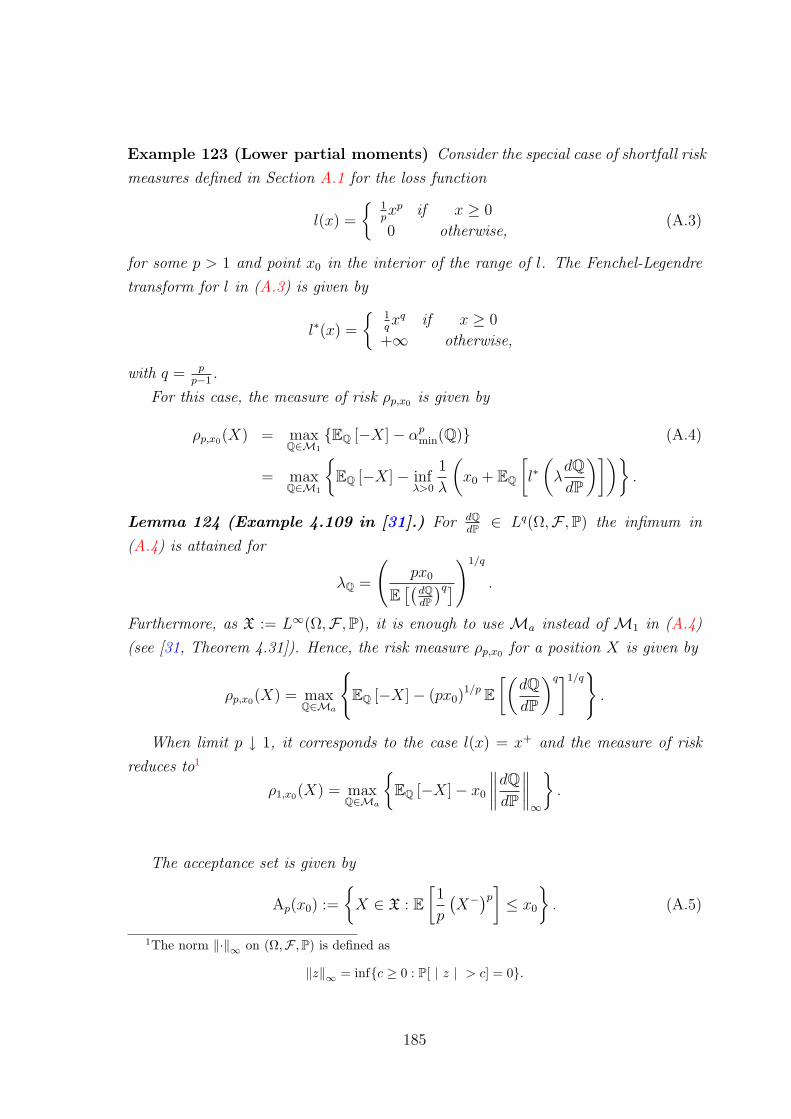
Example 123 (Lower partial moments) Consider the special case of shortfall risk
measures defined in Section A.1 for the loss function
l(x) =
1pxp if x ≥ 0
0 otherwise,(A.3)
for some p > 1 and point x0 in the interior of the range of l. The Fenchel-Legendre
transform for l in (A.3) is given by
l∗(x) =
1qxq if x ≥ 0
+∞ otherwise,
with q = pp−1
.
For this case, the measure of risk ρp,x0 is given by
ρp,x0(X) = maxQ∈M1
EQ [−X]− αpmin(Q) (A.4)
= maxQ∈M1
EQ [−X]− inf
λ>0
1
λ
(x0 + EQ
[l∗(λdQdP
)]).
Lemma 124 (Example 4.109 in [31].) For dQdP ∈ Lq(Ω,F ,P) the infimum in
(A.4) is attained for
λQ =
(px0
E[(
dQdP
)q])1/q
.
Furthermore, as X := L∞(Ω,F ,P), it is enough to use Ma instead of M1 in (A.4)
(see [31, Theorem 4.31]). Hence, the risk measure ρp,x0 for a position X is given by
ρp,x0(X) = maxQ∈Ma
EQ [−X]− (px0)
1/p E[(
dQdP
)q]1/q.
When limit p ↓ 1, it corresponds to the case l(x) = x+ and the measure of risk
reduces to1
ρ1,x0(X) = maxQ∈Ma
EQ [−X]− x0
∥∥∥∥dQdP∥∥∥∥∞
.
The acceptance set is given by
Ap(x0) :=
X ∈ X : E
[1
p
(X−)p] ≤ x0
. (A.5)
1The norm ‖·‖∞ on (Ω,F , P) is defined as
‖z‖∞ = infc ≥ 0 : P[ | z | > c] = 0.
185

And the hedging problem for a liability HT ≥ 0 at time T becomes: For a given
initial capital x0 find a hedging strategy (v, π), π ∈ A(v) such that minimises the
expected shortfall risk for the loss function l under the cost constraint v ≤ x0. Or,
find π ∈ A(v) such that attains the infimum in
infπ∈A(v)
E[1
p
((HT − V
(v,π)T
)+)p]
,
under the cost constraint
supQ∈M1
EQ [HT ] ≤ x0.
One popular approach for the valuation and hedging of contingent claims when
markets are incomplete is the utility maximisation/indifference pricing approach. In
order to show its relation with shortfall risk measures and their associated hedging
problems, we present the example of the entropic measure of risk which corresponds
to the exponential utility function.
Example 125 (Entropic risk measure and exponential utility maximisation)
Consider similar assumptions as in Example 2 but with an acceptance set given by
Aexp(x0) :=X ∈ X : such that E
[e−βX
]≤ x0
,
with x0 an interior point in the range of the functione−βX . It defines the entropic
measure of risk as
ρx0exp(X) := infm ∈ R : E
[e−β(m+X)
]≤ x0 =
1
β
log E
[e−βX
]− log x0
.
This is a convex measure of risk with representation
ρx0exp(X) = sup
Q∈M1
EQ [−X]− αmin(Q) , (A.6)
where M1 denotes the set of all probability measures,
αmin(Q) =1
βH(Q | P)− log x0 =
1
β
EQ
[log
dQdP
]− log x0
and H(Q | P) is the entropy between the measures Q and P. The upper bound in (A.6)
is attained by a measure with density
e−βX
E [e−βX ].
186
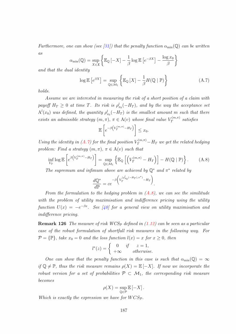
Furthermore, one can show (see [31]) that the penalty function αmin(Q) can be written
as
αmin(Q) = supX∈X
EQ [−X]− 1
βlog E
[e−βX
]− log x0
β
and that the dual identity
log E[eβX]
= supQ∈M1
EQ [X]− 1
βH(Q | P)
(A.7)
holds.
Assume we are interested in measuring the risk of a short position of a claim with
payoff HT ≥ 0 at time T . Its risk is ρlx0
(−HT ), and by the way the acceptance set
Al(x0) was defined, the quantity ρlx0
(−HT ) is the smallest amount m such that there
exists an admissible strategy (m,π), π ∈ A(v) whose final value V(m,π)T satisfies
E[e−β“V
(m,π)T −HT
”]≤ x0.
Using the identity in (A.7) for the final position V(m,π)T −HT we get the related hedging
problem: Find a strategy (m,π), π ∈ A(v) such that
infVT
log E[e
β“V
(m,π)T −HT
”]= sup
Q∈M1
EQ
[(V
(m,π)T −HT
)]−H(Q | P)
. (A.8)
The supremum and infimum above are achieved by Q∗ and π∗ related by
dQ∗
dP= ce
−β
V
(ρlx0
(−HT ),π∗)
T −HT
!.
From the formulation to the hedging problem in (A.8), we can see the similitude
with the problem of utility maximisation and indifference pricing using the utility
function U(x) = −e−βx. See [40] for a general view on utility maximisation and
indifference pricing.
Remark 126 The measure of risk WCSP defined in (1.12) can be seen as a particular
case of the robust formulation of shortfall risk measures in the following way. For
P = P, take x0 = 0 and the loss function l(x) = x for x ≥ 0, then
l∗(z) =
0 if z = 1,
+∞ otherwise.
One can show that the penalty function in this case is such that αmin(Q) = ∞if Q 6= P, thus the risk measure remains ρ(X) = E [−X]. If now we incorporate the
robust version for a set of probabilities P ⊂ M1, the corresponding risk measure
becomes
ρ(X) = supQ∈P
E [−X] .
Which is exactly the expression we have for WCSP .
187
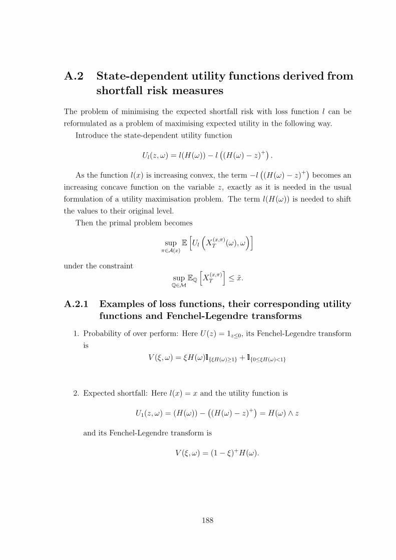
A.2 State-dependent utility functions derived from
shortfall risk measures
The problem of minimising the expected shortfall risk with loss function l can be
reformulated as a problem of maximising expected utility in the following way.
Introduce the state-dependent utility function
Ul(z, ω) = l(H(ω))− l((H(ω)− z)+) .
As the function l(x) is increasing convex, the term −l((H(ω)− z)+) becomes an
increasing concave function on the variable z, exactly as it is needed in the usual
formulation of a utility maximisation problem. The term l(H(ω)) is needed to shift
the values to their original level.
Then the primal problem becomes
supπ∈A(x)
E[Ul
(X
(x,π)T (ω), ω
)]under the constraint
supQ∈M
EQ
[X
(x,π)T
]≤ x.
A.2.1 Examples of loss functions, their corresponding utilityfunctions and Fenchel-Legendre transforms
1. Probability of over perform: Here U(z) = 1z≤0, its Fenchel-Legendre transform
is
V (ξ, ω) = ξH(ω)lξH(ω)≥1 + l0≤ξH(ω)<1
2. Expected shortfall: Here l(x) = x and the utility function is
U1(z, ω) = (H(ω))−((H(ω)− z)+) = H(ω) ∧ z
and its Fenchel-Legendre transform is
V (ξ, ω) = (1− ξ)+H(ω).
188
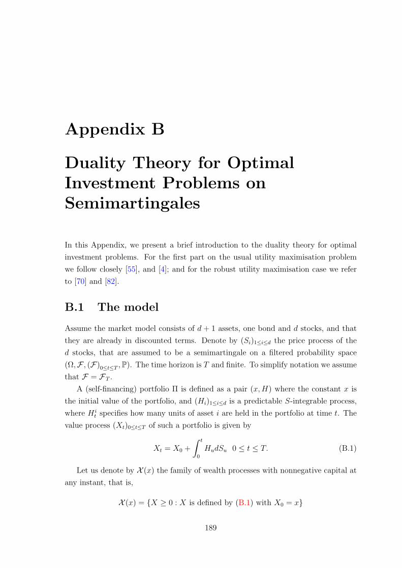
Appendix B
Duality Theory for OptimalInvestment Problems onSemimartingales
In this Appendix, we present a brief introduction to the duality theory for optimal
investment problems. For the first part on the usual utility maximisation problem
we follow closely [55], and [4]; and for the robust utility maximisation case we refer
to [70] and [82].
B.1 The model
Assume the market model consists of d + 1 assets, one bond and d stocks, and that
they are already in discounted terms. Denote by (Si)1≤i≤d the price process of the
d stocks, that are assumed to be a semimartingale on a filtered probability space
(Ω,F , (F)0≤t≤T ,P). The time horizon is T and finite. To simplify notation we assume
that F = FT .
A (self-financing) portfolio Π is defined as a pair (x,H) where the constant x is
the initial value of the portfolio, and (Hi)1≤i≤d is a predictable S-integrable process,
where H it specifies how many units of asset i are held in the portfolio at time t. The
value process (Xt)0≤t≤T of such a portfolio is given by
Xt = X0 +
∫ t
0
HudSu 0 ≤ t ≤ T. (B.1)
Let us denote by X (x) the family of wealth processes with nonnegative capital at
any instant, that is,
X (x) = X ≥ 0 : X is defined by (B.1) with X0 = x
189
We make the following assumption on the family of equivalent local martingale
measures M,
M 6= ∅. (B.2)
This condition is intimately related to the absence of arbitrage opportunities on
the security market. See [17] for precise statements and references.
We also consider that an investor models her preferences via a utility function
U : R → R ∪ ±∞ for wealth at maturity time T . The assumptions on the utility
function are as follows.
Assumption 127 (Usual Regularity Conditions) A utility function U : R →R ∪ ±∞ satisfies the usual regularity conditions if it is increasing on R, continuous
on U > −∞, differentiable and strictly concave on the interior of U > −∞, and
satisfies
U ′(∞) = limx→∞
U ′(x) = 0.
Denoting by dom(U) the interior of U > −∞, we assume that we have one of
the two following cases.
Case 128 (negative wealth not allowed) In this case dom(U) = (0,∞) and as-
sume that U satisfies the conditions
U ′(0) = limx0
U ′(x) = ∞.
Case 129 (negative wealth allowed) In this case dom(U) = R, we assume
U ′(−∞) = limx−∞
U ′(x) = ∞.
B.2 The single prior case
B.2.1 The primal problem
For a given initial capital x > 0, the investor’s objective is to to maximise the expected
value of terminal utility. The value function of this problem is denoted by
u(x) = supX∈X (x)
E [U(XT )] . (B.3)
Intuitively speaking, the value function u plays the role of the utility function of the
investor at time 0, if she subsequently invests in an optimal way. To exclude trivial
cases in (B.3) we shall assume that the value function u is not degenerate:
Assumption 130
u(x) < supξU(ξ), for some x ∈ dom(U).
190
B.2.2 The dual problem
A well-known tool to the study of optimisation problem is the use of duality relation-
ships. In our setting, the dual relation is among the space of convex functions and
semimartingales.
The Fenchel-Legendre transform (or conjugate function) of the utility function U
is defined as
V (y) = supdom(U)
[U(x)− xy] , y > 0,
where dom(U) denotes the domain of definition of the utility function U.
It is well known (see, e.g. [73]) that if U satisfies the hypotheses stated above
then V is a continuously differentiable, decreasing, strictly convex function satisfying
V ′(0) = −∞, V ′(∞) = 0, V (0) = U(∞) and V (∞) = U(0), and also the following
relation holds true
U(x) = infy>0
[V (x) + xy] , x ∈ dom(U).
The derivative of U and V are related as
U ′(x) = y ⇐⇒ x = −V ′(y).
Define the set Y of nonnegative semimartingales, which represents the dual set of
X in the following sense
Y = Y ≥ 0 : Y0 = 1 and XY is a supermartingale for all X ∈ X.
The set Y contains the density process for all Q∈M. For y > 0, define
Y(y) = yY = yY : Y ∈ Y,
and consider the following optimisation problem called the Dual problem
v(y) = supY ∈Y(y)
E [V (YT )] . (B.4)
B.2.3 Relation between the primal and dual problem
In this section, we present some results based on the first case in Assumption 127.
For the general case when negative wealth is allowed we refer to [54, Theorem 2.2],
and [64] when random endowment is permitted.
The primal and dual value functions u(x) and v(y), respectively, are related as
conjugates. This is established in [54, Theorem 2.1] and recalled below.
191
Theorem 131 Suppose that (B.2), Assumption 127 first case and
u(x) <∞ for some x > 0
hold. Then,
1. u(x) <∞ for all x > 0, and there exists y0 ≥ 0 such that v(y) is finitely valued
for y > y0. The value functions u and v are conjugate
v(y) = supdom(u)
[u(x)− xy] , y > 0
u(x) = infy>0
[v(y) + xy] , x ∈ dom(u).
The function u is continuously differentiable on (0,∞) and the function v is strictly
convex on v <∞. The functions u and v satisfy
u′(0) = limx→0
u′(x) = ∞ and v′(∞) = limy→∞
v′(y) = 0.
The optimal solution Y (y) ∈ Y(y) to (B.4) exists and is unique provided that
v(y) <∞.
Definition 132 A utility function U satisfying Assumption 127 is said to have “rea-
sonable asymptotic elasticity” if
AE+∞(U) = lim supx→∞
xU ′(x)
U(x)< 1
and, in case 2 of Assumption 127, we also have
AE−∞(U) = lim supx→−∞
xU ′(x)
U(x)> 1.
Focused on the first case in Assumption 127, in [54, Theorem 2.2], it was shown
that the assumption on “reasonable asymptotic elasticity” is sufficient for the ex-
istence of an optimal solution X ∈ X (x) to the primal problem (B.3) and the
function u is increasing, strictly concave, continuously differentiable and such that
u′(0) = ∞, and u′(∞) = 0. Furthermore, the value function to the dual problem has
the representation
v(y) = infQ∈Me
E[V
(ydQdP
)], (B.5)
where dQdP denotes the Radon-Nikodym derivative of Q with respect to P on FT .
Furthermore, in [55, Theorem 2] the necessary condition for the existence solution
to the primal problem was also analysed and recalled below
192
Theorem 133 Suppose that (B.2), Assumption 127 first case and
v(y) <∞ for all y > 0
hold. Then in addition to the assertions of Theorem 131, we have the following
1. The value functions u and −v are continuously differentiable, increasing and
strictly concave on (0,∞) and satisfy
u′(∞) = limx→∞
u′(x) = 0
−v′(0) = limy→0
−v′(y) = ∞.
2. The optimal solution X(x) ∈ X (x) to (B.3) exists, for any x > 0, and is unique.
In addition, if y = u′(x) then
U ′(XT (x)) = YT (y),
where Y (y) ∈ Y(x) is the optimal solution to (B.4). Moreover, the process
X(x)Y (y) is a martingale.
3. The dual value function v satisfies (B.5).
B.3 The robust utility maximisation case
With the same model setup as in section B.1, in the robust version of the utility max-
imisation problem we need to formulate conditions on the subset P of all probability
measures from which the robust utility functional will be defined.
Assumption 134 The set P satisfies
a) P is convex,
b) P [A] = 0 for some A ∈ Ω if and only if Q [A] = 0 for all Q ∈P,
c) the set
dQdP : Q ∈P
is weakly compact in L1(P).
This set of assumptions are equivalent to the ones in [82] as we discuss next. In
[82] the assumptions needed are the following set.
It is necessary that each measure Q ∈P respects P-null sets, for otherwise a
stochastic integral defined with respect to P might make no sense under Q, this
means we need,
193

1. Q << P for all Q ∈P (this means if for A ∈ Ω, P [A] = 0 then Q [A] = 0 and
Q =fP for some f).
Without loss of generality we can assume,
2. P is convex.
For practical purposes, one may need that the measure attaining the optimum
in the robust utility case also belongs to the set P . In this way, one could treat
the problem as an usual utility maximisation problem on the least favourable
measure. This is achieved if
3. P is closed in some reasonable topology such as total variation (the set
dQdP : Q ∈P
is closed in L0(P)).
If furthermore, we need to guarantee the existence of the least favourable mea-
sure, we need to assume
4. P is relatively compact in a reasonable topology.
Finally, an assumption on the ”sensitivity” in the set P is that
5. Q [A] = 0 for all Q ∈P implies P [A] = 0.
The equivalence in the set of assumptions becomes clear as, number 1 and number
5 imply part a) in Assumption 134; part b) in Assumption 134 is slightly weaker than
Q ∼ P for Q ∈P. On the other hand, assuming c) and b) in Assumption 134 implies
number 1 and Me 6= ∅. And the parts a), b) and c) in Assumption 134 hold if and
only if the set
dQdP : Q ∈P
is weakly compact in L1(P).
B.3.1 The multiple priors primal problem
By the assumptions in the preceding section for each Q ∈P one can associate a random
variable dQdP |FT
at the final time T, and thus by identification a density process dQdP |Ft
,0 ≤ t ≤ T that defines the change of measure.
Denote by DiT := dQi
dP |FT(hence (Di
t)0≤t≤T ) the density process for Qi∈P and by
ZjT := dQj
dP |FT(hence
(Zj
t
)0≤t≤T
) the density processes corresponding to Qj∈Me.
Take
Zji (T ) :=
ZjT
DiT
.
The process(Zj
i (t))0≤t≤T
is a Qj-local martingale.
194
Let Qi∈P be fix momentarily. The usual primal value function for the utility
maximisation problem under the measure Qi is given by
uQi(x) = supX∈X (x)
EQi [U(XT )] .
Now, as we want to incorporate the set of priors P , instead of defining the primal
problem under a specific Qi∈P we need to have it defined on the least favourable
probability measure in P , this is,
u(x) = supX∈X (x)
infQi∈P
EQi [U(XT )] . (B.6)
B.3.2 The multiple priors dual problem
For the dual problem, consider as before the densities DiT , Zj
T and Zji (T ). The dual
value function for the utility maximisation problem under a fixed measure Qi∈P is
vQi(λ) = infQj∈Me
E
[Di
TV
(λZj
T
DiT
)]= inf
Qj∈Me
E[Di
TV(λZj
i (T ))].
Thus, the dual value function of the robust utility maximisation problem is given as
v(λ) := infQi∈P
vQi(λ) = infQi∈P
infQj∈Me
E[Di
TV(λZj
i (T ))],
where the function V (y) is the Fenchel-Legendre transform of U.
B.3.3 Relation between the primal and dual problem
In previous section we recall that necessary and sufficient conditions for the existence
of optimal strategies is the finiteness of the dual value function vQi(λ) for Qi∈Me.
As shown in [82], this condition translates in the robust setting as
vQi(λ) <∞ for all y > 0 and each Qi∈Me. (B.7)
But this condition holds as soon as vQi(λ) is finite for all Qi∈Me and the asymptotic
elasticity of the utility function AE(U) is strictly less than one. While it is sufficient
to assume (B.7) when all measures in P are equivalent to P, we need to assume
AE(U) < 1 to get some regularity results in the general case.
The main results in the robust case are exposed in the next theorem from [82,
Theorem 2.6].
195
Theorem 135 In addition to Assumption 134 assume (B.7). Then both value func-
tions u and v take only finite values and satisfy
u′(∞−) = 0 and v′(0+) = −∞.
For any x > 0 there exists an optimal strategy X ∈ X (x) and a measure Q ∈P such
that
u(x) = infQ∈P
E[U(XT )
]= EQ
[U(XT )
]= uQ(x).
In particular, the supremum and infimum in the primal value function in (B.6) are
attained. There also exist some y in the superdifferental of u(x) and some Y ∈ YP(y)
such that,
v(y) = E[ZV
(YT
Z
)], and XT = I
(YT
Z
)Q-a.s.,
where Z = dQdP and I = −V ′. Furthermore, XY is a martingale under P, and the dual
value function satisfies
v(y) = infQ∗∈Me
infQ∈Me
E[V
(ydQ∗
dQ
)].
If in addition AE(U) < 1 holds, then u is strictly concave and v is continuously
differentiable. Moreover, XTYT is supported by Z > 0, i.e.,XTYT > 0
= Z > 0 P-a.s.
And if all measures in P are equivalent to P we have from [82, Corollary 2.7].
Corollary 136 In addition to the assumptions in previous theorem, let us assume
(B.7) and that all measures in P are equivalent to P. Then both value functions u and
v take only finite values, u is strictly concave, and v is continuously differentiable.
Then for each y > 0 such that v(y) >∞ there exist Q ∈P and Y ∈ YQ(y) such that
v(y) = EQ
[V(YT
)].
Moreover, Y is unique: any other optimal pair (Q′, Y ′) ∈ (Q, Y ) : Q ∈P,Y ∈ YQ(y)satisfies Y ′ = Y P-a.s.
On the other hand, for any x > 0, the optimal solution X ∈ X (x) is unique and
it is given by
XT = I(YT ),
where I is the inverse function of U ′ and Y is as above for y as in previous theorem.
196
B.4 Proof of Lemma 107
In this section we check that all conditions in [82, Theorem 2.2] are satisfied.
Proof. For the conditions on the utility function we have that the functions Uε(x) :
R → R, and Uε(x) : R → R are strictly increasing, strictly concave and continuously
differentiable. In relation with the no random endowment case, our assumption in
(5.7) about Xt ≥ 0 makes sure the functions take only nonnegative values. For the
random endowment case, the condition in (5.7) and Assumption 116 on the bound-
edness of the payoff function H(y) guarantees that XT +H(YT ) > 0 (see [39]), then
the functions also only take values in (0,∞).
The Inada conditions are:
limx→−∞+
Uε′(x) = +∞, limx→+∞−
Uε′(x) = 0 and Uε′(0) = 1.
and
limx→−∞+
Uε′(x) = 1, limx→+∞−
Uε′(x) = 0 and Uε′(0) = 1/2.
For the function Uε(x), the Inada condition at −∞ (or zero) are not fully satisfied,
but it is not needed as explained in [75, p. 13 and Sec. 6], arguing that we can
always approximate a given utility function uniformly to within any given ε > 0 by
one satisfying the Inada condition at −∞ (or zero). With respect to the asymptotic
elasticity defined as
AE−∞(U) = lim infx→−∞
xU ′(x)U(x)
AE+∞(U) = lim supx→+∞
xU ′(x)U(x)
,
we have
AE−∞(Uε) = +∞ > 1, AE+∞(Uε) = −∞ < 1,
and
AE−∞(Uε) = 1, AE+∞(Uε) = −∞ < 1, but limx→0+
xUε′(x)Uε(x)
< 1.
For the set of assumptions regarding the set P , we have that P[A] = 0 if and only
if Q[A] = 0 for all Q ∈ P , as P is a subset of Me. That the set
dQdP : Q ∈ P
is
convex and closed in L0(P) follows from [43, Lemma 3.1]. In [43] P is a subset of
Ma, which is more general than in our setting.
197
Appendix C
Selecting a Measurable Function
Let
z = (z1, ..., zp) ∈ Rp and u = (u1, ..., um) ∈ Rm,
for p and m two positive integers. Denote by (z, u) the elements in Rp+m. For a set
D ⊂ Rp+m, let
Dz = u : (z, u) ∈ D, ∆ = z : Dz is not empty.
We callD to be σ-compact ifD = D1∪D2∪... whereD1, D2, ... are compact sets (every
open and closed set is σ-compact). By “almost all z” we mean except for a set of
p-dimensional Lebesgue measure 0. A vector valued function u(z) = (u1(z), ..., um(z))
is measurable if and only if each component ui is measurable. By changing a Lebesgue
measurable function u on a set of p-dimensional measure 0, we can arrange that u is
Borel measurable.
Lemma 137 ([25, Lemma B]) If D is σ-compact, then there exists a measurable
function u = u(z) with (z, u(z)) ∈ D for almost all z ∈ ∆.
Proof. See [25, Lemma B].
198
Appendix D
Some Results Related with supand inf of Sets and Functions
Definition 138 Let A be a nonempty set of the affinely extended real numbers R :=
R ∪ ±∞, the supremum of A, denoted by supA is defined as
supA := minr ∈ R : ∀a ∈ A, a ≤ r
.
Proposition 139 Let A ⊆ R nonempty. Then supA satisfies ∀a ∈ A, a ≤ supA
and for any arbitrary ε > 0 there exists a ∈ A such that a > supA− ε.
Proof. Suppose there does not exist a ∈ A for which a > supA− ε, but this implies
that supA− ε is an upper bound for the set A and clearly supA− ε < supA, which
contradicts the fact that supA is the least upper bound for the set A. Conversely,
assume M ∈ R is such that M > supA and ∀a ∈ A, a ≤ M and a ≤ supA. Take
ε < supA −M , then there exists an a ∈ A for which a > supA − ε > M , but this
inequality contradicts the assumption that M is an upper bound for the set A.
Lemma 140 Let A and B two subsets of R, then
supA+B = supA+ supB
Proof. For any a ∈ A and b ∈ B, we have a ≤ supA and b ≤ supB, thus a + b ≤supA+ supB. This means that supA+ supB is an upper bound for the set A+B.
Now, take ε > 0 and by By Proposition 139 there exist a ∈ A and b ∈ B such that
supA−ε/2 < a and supA−ε/2 < a, which together give us supA+supB−ε < a+b.
Using again Proposition 139 on the set A + B, we conclude that supA + supB =
supA+B.
199

Lemma 141 For two nonempty sets A ⊆ B ⊆ R, we have
supA ≤ supB
Proof. Take any a ∈ A, and as a also belongs to B then a ≤ supB, which implies
that supB is an upper bound of the set A, but from the Definition 138, supA ≤ supB.
Lemma 142 For two nonempty sets A ⊆ B ⊆ R, suppose there exists a ∈ A such
that a = supB, then
supA = supB.
Proof. As a ∈ A we have a ≤ supA, thus supB ≤ supA, and by Lemma 141 we get
the equality.
Lemma 143 Let f and g two real continuous functions with domain D, then
supx∈D
f(x) + g(x) ≤ supx∈D
f(x) + supx∈D
g(x).
Proof. Define
A := f(x) : x ∈ D
B := g(x) : x ∈ D
C := f(x) + g(x) : x ∈ D .
clearly C ⊆ A+B, applying Lemma 141 and Lemma 140 we have supC ≤ supA+B =
supA+ supB.
Lemma 144 Let f and g two continuous real functions with compact domain D. If
x ∈ D is such that
f(x) = supx∈D
f(x)
g(x) = supx∈D
g(x).
Then
supx∈D
f(x) + g(x) = supx∈D
f(x) + supx∈D
g(x)
Proof. It follow immediately by using Lemma 141, Lemma 140 and Lemma 142.
200
References
[1] Abraham, R., Marsden, J. E., and Ratiu, T. (1988). Manifolds, tensor analysis,
and applications, volume 75 of Applied Mathematical Sciences. Springer-Verlag,
New York.
[2] Acerbi, C. and Tasche, D. (2002). On the coherence of expected shortfall.
arXiv:cond-mat/0104295 v5.
[3] Artzner, P., Delbaen, F., Eber, J.-M., and Heath, D. (1999). Coherent measures
of risk. Math. Finance, 9(3):203–228.
[4] Back, K., Bielecki, T. R., Hipp, C., Peng, S., and Schachermayer, W. (2004).
Stochastic methods in finance, volume 1856 of Lecture Notes in Mathematics.
Springer-Verlag, Berlin.
[5] Barrieu, P. and El Karoui, N. (2005). Indifference Pricing, chapter Pricing, hedg-
ing and optimally designing derivatives via minimization of risk measures. Prince-
ton University Press.
[6] Bertsekas, D. P. and Shreve, S. E. (1978). Stochastic optimal control, volume 139
of Mathematics in Science and Engineering. Academic Press Inc. [Harcourt Brace
Jovanovich Publishers], New York.
[7] Cheridito, P. and Summer, C. (2006). Utility maximization under increasing risk
aversion in one-period models. Finance Stoch., 10(1):147–158.
[8] Cisneros-Molina, M. (2005). On explicit computation of transition probability
densities for some transformed markov diffusion processes. Working paper.
[9] Cvitanic, J. (2000). Minimizing expected loss of hedging in incomplete and con-
strained markets. SIAM J. Control Optim., 38(4):1050–1066 (electronic).
[10] Cvitanic, J. and Karatzas, I. (1999). On dynamic measures of risk. Finance
Stoch., 3(4):451–482.
201
[11] Cvitanic, J., Schachermayer, W., and Wang, H. (2001). Utility maximization in
incomplete markets with random endowment. Finance Stoch., 5(2):259–272.
[12] Davis, M. (1998). A note on the forward measure. Finance and Stochastics, 2:19
– 28.
[13] Davis, M. (2000a). Optimal hedging with basis risk.
[14] Davis, M. (2000b). Option valuation and hedging with basis risk. In System
theory: modeling, analysis and control (Cambridge, MA, 1999), volume 518 of
Kluwer Internat. Ser. Engrg. Comput. Sci., pages 245–254. Kluwer Acad. Publ.,
Boston, MA.
[15] Delbaen, F. (2000). Coherent risk measures. Cattedra Galileiana. [Galileo Chair].
Scuola Normale Superiore, Classe di Scienze, Pisa.
[16] Delbaen, F. (2002). Coherent risk measures on general probability spaces. In
Advances in finance and stochastics, pages 1–37. Springer, Berlin.
[17] Delbaen, F. and Schachermayer, W. (2005). The Mathematics of Arbitrage.
Springer-Verlag.
[18] Detlefsen, K. and Scandolo, G. (2005). Conditional and dynamic convex risk
measures. Finance Stoch., 9(4):539–561.
[19] Duffie, D. and Pan, J. (1997). An overview of value at risk. The Journal of
Derivatives, 1:7–49.
[20] El Karoui, N. and Quenez, M.-C. (1995). Dynamic programming and pricing of
contingent claims in an incomplete market. SIAM J. Control Optim., 33(1):29–66.
[21] Elliot, R. J. and Kopp, P. E. (1999). Mathematics of financial markets. Springer.
[22] Elliott, R., Siu, T., and Yang, H. (2003). On a generalized form of risk measure.
University of Hong Kong Preprint Series, (364 (7/03)).
[23] Favero, G. (2001). Shortfall risk minimization under model uncertainty in
the binomial case: adaptive and robust approaches. Math. Methods Oper. Res.,
53(3):493–503.
[24] Fischer, T. (2003). Risk capital allocation by coherent risk measures based on
one-sided moments. Insurance Math. Econom., 32(1):135–146.
202
[25] Fleming, W. H. and Rishel, R. W. (1975). Deterministic and stochastic optimal
control. Springer-Verlag, Berlin.
[26] Fleming, W. H. and Soner, H. M. (2006). Controlled Markov processes and viscos-
ity solutions, volume 25 of Stochastic Modelling and Applied Probability. Springer,
New York.
[27] Follmer, H. and Leukert, P. (1999). Quantile hedging. Finance Stoch., 3(3):251–
273.
[28] Follmer, H. and Leukert, P. (2000). Efficient hedging: cost versus shortfall risk.
Finance Stoch., 4(2):117–146.
[29] Follmer, H. and Schied, A. (2002a). Convex measures of risk and trading con-
straints. Finance Stoch., 6(4):429–447.
[30] Follmer, H. and Schied, A. (2002b). Robust preferences and convex measures of
risk. In Advances in finance and stochastics, pages 39–56. Springer, Berlin.
[31] Follmer, H. and Schied, A. (2002c). Stochastic finance, volume 27 of de Gruyter
Studies in Mathematics. Walter de Gruyter & Co., Berlin.
[32] Follmer, H. and Schied, A. (2004). Stochastic finance, volume 27 of de Gruyter
Studies in Mathematics. Walter de Gruyter & Co., 2nd. Edition, Berlin.
[33] Fremlin, D. H. (2002). Measure Theory, volume 3. Torres Fremlin publisher.
[34] Frittelli, M. and Gianin, R. (2002). Putting order in risk measures. Journal of
Banking and Finance, 26:1473–1486.
[35] Frittelli, M. and Gianin, R. (2004). Dynamic convex risk measures. In Szego, G.,
editor, Risk Measures for the 21st Century, pages 227–248. John Wiley and Sons.
[36] Goll, T. and L., R. (2001). Minimax and minimal distance martingele measures
and their relationship to portfolio optimization. Finance and Stochastics, 5:557–
581.
[37] Gundel, A. (2005). Robust utility maximization for complete and incomplete
market models. Finance Stoch., 9(2):151–176.
[38] Heath, D. and Schweizer, M. (2000). Martingales versus PDEs in finance: an
equivalence result with examples. J. Appl. Probab., 37(4):947–957.
203
[39] Henderson, V. (2002). Valuation of claims on nontraded assets using utility
maximization. Math. Finance, 12(4):351–373.
[40] Henderson, V. and Hobson, D. (2004). Utility indifference pricing - an overview.
In Indifference pricing. Princeton University Press.
[41] Henderson, V. and Hobson, D. G. (2002). Real options with constant relative
risk aversion. J. Econom. Dynam. Control, 27(2):329–355.
[42] Hernandez-Hernandez, D. and Schied, A. (2006a). A control approach to robust
utility maximization with logarithmic and time-consistent penalties.
[43] Hernandez-Hernandez, D. and Schied, A. (2006b). Robust utility maximization
in a stochastic factor model. Statistics and Decisions. Special Volume on Risk
Measures, 24.
[44] Hobson, D. and Jeremy, P. (2005). Maximizing the probability of a perfect hedge
using an imperfectly correlated instrument. International Journal of Theoretical
and Applied Finance.
[45] Hobson, D. G. (2005). Bounds for the utility-indifference prices of non-traded
assets in incomplete markets. Decis. Econ. Finance, 28(1):33–52.
[46] Hubalek, F. and Sachermeyer, W. (1999). The limitations of no-arbitrage ar-
guments for real options. Adaptative Information Systems and Modelling in Eco-
nomics and Management Science. Working paper series, (58).
[47] Jacod, J. and Shiryaev, A. N. (2003). Limit theorems for stochastic processes, vol-
ume 288 of Grundlehren der Mathematischen Wissenschaften [Fundamental Prin-
ciples of Mathematical Sciences]. Springer-Verlag, Berlin.
[48] Jaschke, S. (2002). Quantile var is the wrong measure to quantify market risk
for regulatory purposes. Research report, Weierstrass Institute.
[49] Jonsson, M. and Sircar, K. R. (2002). Partial hedging in a stochastic volatility
environment. Math. Finance, 12(4):375–409.
[50] Jouini, E. and Napp, C. (2004). Convergence of utility functions and convergence
of optimal strategies. Finance Stoch., 8(1):133–144.
[51] Karatzas, I. and Shreve, S. E. (1988). Brownian motion and stochastic calculus,
volume 113 of Graduate Texts in Mathematics. Springer-Verlag, New York.
204
[52] Karatzas, I. and Shreve, S. E. (1998). Methods of mathematical finance, vol-
ume 39 of Applications of mathematics: Stochastic modelling and applied probabil-
ity. Springer-Verlag.
[53] Kloeden, P. E. and Platen, E. (1992). Numerical solution of stochastic differential
equations, volume 23 of Applications of Mathematics (New York). Springer-Verlag,
Berlin.
[54] Kramkov, D. and Schachermayer, W. (1999). The asymptotic elasticity of util-
ity functions and optimal investment in incomplete markets. Annals of Applied
Probability, 9(3):904–950.
[55] Kramkov, D. and Schachermayer, W. (2003). Necessary and sufficient conditions
in the problem of optimal investment in incomplete markets. Ann. Appl. Probab.,
13(4):1504–1516.
[56] Kratschmer, V. (2005). Robust representation of convex risk measures by prob-
ability measures. Finance Stoch., 9(4):597–608.
[57] Lapeyre, B., Agnes, S., and Talay, D. (2006). Simulation of Financial Models:
Mathematical Foundations and Applications.
[58] Monoyios, M. (2004). Performance of utility-based strategies for hedging basis
risk. Quant. Finance, 4(3):245–255.
[59] Musiela, M. and Rutkowski, M. (1997). Martingale Methods in Financial Mod-
eling. Springer-Verlag.
[60] Musiela, M. and Zariphopoulou, T. (2004a). An example of indifference prices
under exponential preferences. Finance Stoch., 8(2):229–239.
[61] Musiela, M. and Zariphopoulou, T. (2004b). A valuation algorithm for indiffer-
ence prices in incomplete markets. Finance Stoch., 8(3):399–414.
[62] Øksendal, B. (1991). Stochastic control theory—a brief summary. In Stochastic
models and option values (Loen, 1989), volume 200 of Contrib. Econom. Anal.,
pages 19–29. North-Holland, Amsterdam.
[63] Øksendal, B. (1995). Stochastic Differential Equations. An Introduction with
Applications. Springer Verlag.
205
[64] Owen, M. P. (2002). Utility based optimal hedging in incomplete markets. Ann.
Appl. Probab., 12(2):691–709.
[65] Palmowski, Z. and Rolski, T. (2002). A technique for exponential change of
measure for Markov processes. Bernoulli, 8(6):767–785.
[66] Pflug, G. C. (2000). Some remarks on the value-at-risk and the conditional value-
at-risk. In Probabilistic constrained optimization, volume 49 of Nonconvex Optim.
Appl., pages 272–281. Kluwer Acad. Publ., Dordrecht.
[67] Pham, H. (2000). Dynamic Lp-hedging in discrete time under cone constraints.
SIAM J. Control Optim., 38(3):665–682 (electronic).
[68] Pham, H. (2005). On some recent aspects of stochastic control and their appli-
cations. Probability Surveys, 2:506–549.
[69] Pliska, S. R. (1997). Introduction to mathematical finance: discrete time models.
Blackwell, Oxford.
[70] Quenez, M.-C. (2004). Optimal portfolio in a multiple-priors model. In Seminar
on Stochastic Analysis, Random Fields and Applications IV, volume 58 of Progr.
Probab., pages 291–321. Birkhauser, Basel.
[71] Revuz, D. and Yor, M. (2005). Continuous Martingales and Brownian Motion.
Grundlehren der Mathematischen Wissenchaften. Springer-Verlag, 3rd. edition.
[72] Rockafellar, R. and Uryaser, S. (2002). Conditional value-at-risk for general loss
distributions. Journal of Banking and Finance, 26(7):1443–1471.
[73] Rockafellar, R. T. (1970). Convex analysis. Princeton Mathematical Series, No.
28. Princeton University Press, Princeton, N.J.
[74] Rockafellar, R. T. and Uryaser, S. (2000). Optimization of conditional value-at-
risk. Journal of Risk, 2:21–41.
[75] Rogers, L. C. G. (2001). Duality in constrained optimal investment and con-
sumption problems: a synthesis.
[76] Rogers, L. C. G. and Williams, D. (2000a). Diffusions, Markov processes,
and martingales. Vol. 1. Cambridge Mathematical Library. Cambridge University
Press, Cambridge, 2nd. edition.
206

[77] Rogers, L. C. G. and Williams, D. (2000b). Diffusions, Markov processes,
and martingales. Vol. 2. Cambridge Mathematical Library. Cambridge University
Press, Cambridge, 2nd. edition.
[78] Rudin, W. (1953). Principles of mathematical analysis. McGraw-Hill Book
Company, Inc., New York-Toronto-London.
[79] Scagnellato, C. and Vargiolu, T. (2002). Explicit solutions for shortfall risk
minimization in multinomial models. Decis. Econ. Finance, 25(2):145–155.
[80] Schied, A. (2005). Optimal investments for robust utility functionals in complete
market models. Math. Oper. Res., 30(3):750–764.
[81] Schied, A. (2006). Risk measures and robust optimization problems. Stoch.
Models, 22(4):753–831.
[82] Schied, A. and Wu, C.-T. (2005). Duality theory for optimal investments under
model uncertainty. Statistics and Decision, 23(3):199–217.
[83] Schulmerich, M. and Trautmann, S. (2003). Local expected shortfall-hedging in
discrete time. European Finance Review, 7:75–102.
[84] Siu, T. K. and Yang, H. (2001). A p.d.e. approach for measuring risk of deriva-
tives. Appl. Math. Finance, 7(3):211–228.
[85] Spivak, G. and Cvitanic, J. (1999). Maximizing the probability of a perfect
hedge. Ann. Appl. Probab., 9(4):1303–1328.
[86] Stroock, D. W. and Varadhan, S. R. S. (1979). Multidimensional diffusion pro-
cesses, volume 233 of Grundlehren der Mathematischen Wissenschaften [Funda-
mental Principles of Mathematical Sciences]. Springer-Verlag, Berlin.
[87] Summer, C. (2002). Utility maximization and Increasing Risk Aversion. PhD
thesis, Vienna University of Technology.
[88] Tak Kuen Siu, H. T. and Yang, H. (2003). On p.d.e. approach for measuring tail
risk of portfolios containing derivatives.
[89] Tasche, D. (2002). Expected shortfall and beyond. In Statistical data analysis
based on the L1-norm and related methods (Neuchatel, 2002), Stat. Ind. Technol.,
pages 109–123. Birkhauser, Basel.
207
[90] Tessitore, G. and Zabczyk, J. (2002). Pricing options for Markovian models.
In Stochastic processes and related topics (Siegmundsburg, 2000), volume 12 of
Stochastics Monogr., pages 249–268. Taylor & Francis, London.
[91] Testuri, C. E. and Uryasev, S. (2004). On relation between expected regret and
conditional value-at-risk. In Handbook of computational and numerical methods in
finance, pages 361–372. Birkhauser Boston, Boston, MA.
[92] Tudor, C. (1994). Procesos estocasticos, volume 2 of Aportaciones Matematicas:
Textos [Mathematical Contributions: Texts]. Sociedad Matematica Mexicana,
Mexico.
[93] Uryasev, S. and Rockafellar, R. (2001). Conditional value-at-risk: optimization
approach. In Stochastic optimization: algorithms and applications (Gainesville, FL,
2000), volume 54 of Appl. Optim., pages 411–435. Kluwer Acad. Publ., Dordrecht.
[94] Xu, M. (2004). Minimizing Shortfall Risk Using Duality Approach - An Ap-
plication to Partial Hedging in Incomplete Markets. PhD thesis, Carnegie Mellon
University.
[95] Yang, H. and Siu, T. K. (2001). Coherent risk measures for derivatives under
Black-Scholes economy. Int. J. Theor. Appl. Finance, 4(5):819–835.
[96] Yong, J. and Zhou, X. Y. (1999). Stochastic controls, volume 43 of Applications
of Mathematics (New York). Springer-Verlag, New York. Hamiltonian systems and
HJB equations.
208