Embed Size (px)
Citation preview
MATHEMATICAL METHODS OF ORGANIZING AND PLANNING PRODUCTION*t
L. V. KANTOROVICH
Leningrad State University
1939
Contents
Editor's Foreword .................................................................. 366 Introduction ...................................................................... 367
I. The Distribution of the Processing of Items by Machines Giving the Maximum Output Under the Condition of Completeness (Formulation of the Basic Mathe- matical Problems) ........................................................ 369
II. Organization of Production in Such a Way as to Guarantee the Maximum Ful- fillment of the Plan Under Conditions of a Given Product Mix ............... 374
III. Optimal Utilization of Machinery ............................................ 377 IV. Minimization of Scrap ....................................................... 379 V. Maximum Utilization of a Complex Raw Material ............................ 382
VI. Most Rational Utilization of Fuel ............................................ 382 VII. Optimum Fulfillment of a Construction Plan with Given Construction Materials. . 383
VIII. Optimum Distribution of Arable Land ........................................ 384 IX. Best Plan of Freight Shipments .............................................. 386
Conclusion ...................................................................... 387 Appendix 1. Method of Resolving Multipliers ........................ 390 Appendix 2. Solution of Problem A for a Complex Case (The problem of the Plywood
Trust) ...................................................................... 410 Appendix 3. Theoretical Supplement (Proof of Existence of the Resolving Multipliers).. 419
FOREWORD
The author of the work "Mathematical Methods of Organizing and Planning Production", Professor L. V. Kantorovich, is an eminent authority in the field of mathematics. This work is interesting from a purely mathematical point of view since it presents an original method, going beyond the limits of classical mathematical analysis, for solving extremal problems. On the other hand, this work also provides an application of mathematical methods to questions of organizing production which merits the serious attention of workers in different branches of industry.
The work which is here presented was discussed at a meeting of the M'Iathe- inatics Section of the Institute of Mathematics and Mechanics of the Leningrad State University, and was highly praised by mathematicians. In addition, a
* Received March 1958. t The editors of Management Science would like to express their very sincere thanks to
Robert W. Campbell and W. H. Marlow who prepared the English translation and to Mrs. Susan Koenigsberg who helped to edit the final manuscript.
366
MATHEMATICAL METHODS OF ORGANIZING AND PLANNING PRODUCTION 367
special meeting of industrial workers was called by the Directorate of the Uni- versity at which the other aspect of the work-its practical application-was discussed. The industrial workers unanimously evinced great interest in the work and expressed a desire to see it published in the near future.
The basic part of the present monograph reproduces the contents of the report given at the meetings mentioned above. It includes a presentation of the mathe- matical problems and anl indication of those questions of organization anld planl- ning in the fields of industry, construction, transportation and agriculture which lead to the formulation of these problems. The exposition is illustrated by several specific numerical examples. A lack of time and the fact that the author is a mathematician rather than someone concerned with industrial production, did not permit an increase in the number of these examples or an attempt to make these examples as real and up-to-date as they might be. We believe that., in spite of this, such examples will be extremely useful to the reader for they show the circumstances in which the mathematical methods are applicable and also the effectiveness of their application.
Three appendices to the work contain an exposition and the foundations of the process of solving the indicated extremal problems by the method of the author.
We hope that this monograph will play a very useful role in the development of our socialist industry.
A. R. MARCHENKO
Introduction'
The immense tasks laid down in the plan for the third Five Year Plan period require that we achieve the highest possible productionl on the basis of the opti- mum utilization of the existing reserves of industry: materials, labor and equip- ment.
There are two ways of increasing the efficiency of the work of a shop, an enter- prise, or a whole branlch of industry. One way is by various improvemients in technology; that is, new attachments for individual machines, changes in tech- nological processes, and the discovery of new, better kinds of raw materials. The other way-thus far much less used-is improvement in the organization of planning and production. Here are included, for instance, such questions as the distribution of work among individual machines of the enterprise or among mechanisms, the correct distribution of orders among enterprises, the correct distribution of different kinds of raw materials, fuel, and other factors. Both are clearly mentioned in the resolutions of the 18th Party Congress. There it is stated that "the most important thing for the fulfillment of the goals of the
1 The present work represents a significantly enlarged stenographic record of a report given on May 13, 1939, at the Leningrad State University to a meeting which was also at- tended by representatives of industrial research institutes. Additional material comes from a report devoted specifically to problems connected with construction which was given on May 26, 1939 at the Leningrad Institute for Engineers of Industrial Construction.

368 L. V. KANTOROVICH
program for the growth of production in the Third Five Year Plan period is . . . the widespread development of work to propagate the most up-to-date technology and scientific organization of production."2 Thus the two lines of approach indicated above are specified: as well as the introduction of the most up-to-date technology, the role of scientific organization is emphasized.
In connection with the solution of a problem presented to the Institute of Mathematics and Mechanics of the Leningrad State University by the Labora- tory of the Plywood Trust, I discovered that a whole range of problems of the most diverse character relating to the scientific organization of production (questions of the optimum distribution of the work of machines and mechanisms, the minimization of scrap, the best utilization of raw materials and local ma- terials, fuel, transportation, and so on) lead to the formulation of a single group of mathematical problems (extremal problems). These problems are not directly comparable to problems considered in mathematical analysis. It is more correct to say that they are formally similar, and even turn out to be formally very simple, but the process of solving them with which one is faced [i.e., by mathe- matical analysis] is practically completely unusable, since it requires the solu- tion of tens of thousands or even millions of systems of equations for completion.
I have succeeded in finding a comparatively simple general method of solving this group of problems which is applicable to all the problems I have mentioned, and is sufficiently simple and effective for their solution to be made completely achievable under practical conditions.
I want to emphasize again that the greater part of the problems of which I shall speak, relating to the organization and planning of production, are con- nected specifically with the Soviet system of economy and in the majority of cases do not arise in the economy of a capitalist society. There the choice of output is determined not by the plan but by the interests and profits of indi- vidual capitalists. The owner of the enterprise chooses for production those goods which at a given moment have the highest price, can most easily be sold, and therefore give the largest profit. The raw material used is not that of which there are huge supplies in the country, but that which the entrepreneur can buy most cheaply. The question of the maximum utilization of equipment is not raised; in any case, the majority of enterprises work at half capacity.
In the USSR the situation is different. Everything is subordinated not to the interests and advantage of the individual enterprise, but to the task of fulfilling the state plan. The basic task of an enterprise is the fulfillment and overfulfill- ment of its plan, which is a part of the general state plan. Moreover this not only means fulfillment of the plan in aggregate terms (i.e. total value of output, total tonnage, and so on), but the certain fulfillment of the plan for all kinds of output; that is, the fulfillment of the assortment plan (the fulfillment of the plan for each kind of output, the completeness of individual items of output, and so on).
This feature, the necessity of fulfilling both the overall plan and all its com-
2 Bol'shevikc, 1939 No. 7, p. 14.

MATHEMATICAL METHODS OF ORGANIZING AND PLANNING PRODUCTION 369
TABLE 1 Productivity of the machines for two parts
Output per machine Total output Type of machine machines
First part Second part First part Second part
Milling machines ................ 3 10 20 30 60 Turret lathes .................... 3 20 30 60 90 Automatic turret lathe ........... 1 30 80 30 80
ponent parts, is essential for us, since in the setting of the tasks connected with securing maximum output we must consider the composition and completeness as extremely important supplementary conditions. Also extremely important is the utilization of materials not chosen in some a priori way, but those which are really available, in particular, local materials, and the utilization of ma- terials in accordance with the amount of them produced in the given region. It should be noted that our methods make it possible to solve the problems con- nected precisely with these real conditions and situations.
Now let us pass to an examination of various practical problems of organiza- tion and planning of production and let us ascertain the mathematical prob- lems to which they lead.
I. The Distribution of the Processing of Items by Machines Giving the Maximum Output under the Condition of Completeness (Formula-
tion of the Basic Mathematical Problems) In order to illustrate the character of the problems we have in mind, I cite
one very simple example which requires no special methods for solution since it is clear by itself. This example will play an illustrative role3 and will help to clarify the formulation of the problem.
Example 1. The milling work in producing parts of metal items can be done on different machines: milling machines, turret lathes of a more advanced type, and an automatic turret lathe. For preciseness I shall consider the following problem. There are three milling machines, three turret lathes, and one auto- matic turret lathe. The item to be fabricated-I shall consider an extremely simple case-consists of two parts.
The output of each part is as follows. During a working day it is possible to turn out on the milling machine, 10 of the first part or 20 of the second; on the turret lathe, 20 of the first part or 30 of the second; and on the automatic tur- ret lathe, 30 of the first or 80 of the second. Thus if we consider all the machines (three each of the milling machines and the turret lathes, and one automatic machine), we can if we wish turn out in a day 30 + 60 + 30 of the first part on each type of machine, respectively, or a total of 120 parts on all the machines. Of the second part, we can turn out 60 + 90 + 80. (See Table 1.)
3 Since this problem plays a purely illustrative role, we have not tried to make it realistic; that is, we have not chosen data and circumstances which might occur in reality.

370 L. V. KANTOROVICH
Now we need to solve the following problem: the work is to be divided so as to load the working day of these machines in such a way as to obtainl the maxi- mum output, and at the same time it is important not simply to produce the maximum number of parts, but to find the method of maximum output of com- pleted items, in the given case consisting of two parts. Thus we must divide the work time of each machine in such a way as to obtain the maximum number of finished items.
If no attempt is made to obtain a maximum, but only to achieve completeness, then we could produce both parts on each machine in equal quantities. For this it is sufficient to divide the working day of each machine in such a way that it produces the same number of each part. Then it turns out that the milling ma- chine could produce 20 of the first part and 20 of the second. (Actually, on the milling machines the production of 20 of the second part is equivalent to 10 of the first.) The turret lathes can then produce 36 of the first and 36 of the second; the automatic turret lathe can produce 21 of the first and 21 of the second part; and the total output of all the machines will be 77 of the first and 77 of the second part, or in other words, 77 complete items. (See Table 2.)
Let us now find, in the given example, the most expedient method of opera- tion. We examine the different ratios. On the milling machine, one unit of the first part is equal to two of the second; on the turret lathe, this ratio is 2 to 3; on the automatic machine, 3 to 8. There are various reasons for this; one of the operations can require the same time on each machine, another operation can be performed five times faster on the automatic machine than on the milling machine, and so on. Owing to these conditions, these ratios are different for different machines turning out identical parts. One part can be turned out rela- tively better on one machine, another part on a different machine.
Examination of these ratios immediately leads to the solution. It is necessary to turn out the first part where it is most advantageously produced (on the turret lathe) and the second part should be assigned the automatic machine. As far as the milling machines are concerned, the production of the first and second parts should be partially divided among them in such a way as to obtain the same number of the first and second parts.
If we make an assignment in accordance with this method, the numbers will be as follows: on the milling machine there will be 26 and 6; on the turret lathe only 60 of the first, and none of the secolnd; on the automatic machine 80 of the second, and none of the first. Altogether we will get 86 of the first part and 86 of the second. (Table 2.)
If such a redistribution is made, we will obtain an effect that is not very great, but still appreciable: an increase in output of 11 per cent. Moreover, this in- crease in production occurs with no expenditure whatever.
This problem was solved so easily from elementary considerations because we had only three machines and two parts. Practically, in the majority of cases, one must deal with more complex situations, and to find the solution simply by common sense is hardly possible. It is too much to hope that the ordinary en- gineer, with no calculation of any kind, would happen upon the best solution.

MATHEMATICAL METHODS OF ORGANIZING AND PLANNING PRODUCTION 371
TABLE 2 Distribution of the processing of parts among machines
Simplest solution Optimum solution Type of machines
First part Second part First part Second part
Milling machines ............ 20 20 26 6 Turret lathes ................ 36 36 60 Automatic turret lathe ....... 21 21 - 80
Number of complete sets ... 77 77 86 86
In order to make clear the kind of mathematical problem to which this leads, I shall examine this question in more general form. I shall introduce here several mathematical problems connected with the question of producing items con- sisting of several parts. With respect to all the other fields of application of the mathematical methods which I mentioned above, it turns out that the mathe- matical problems are the same in each case, so that in the other cases it will only be necessary for me to point out which of these problems represents the situa- tion.
Therefore, let us look at the general case. We have a certain number n of machines and on them we turn out items consisting of m different parts. Let us suppose that if we produce the k-th part on the i-th machine we can produce in a day ai,k parts. These are the given data. (Let us note that if it is impossible to turn out the k-th part on the i-th machine, then it is necessary to set the corre- sponding aei,k = 0.)
Now what do we need? It is necessary to distribute the work of making the parts among machines in such a way as to turn out the largest number of com- pleted items. Let us designate by hi,k the time (expressed as a fraction of the working day) that we are going to use the i-th machine to produce the k-th part. This time is unknown; it is necessary to determine it on the basis of the condi- tion of obtaining the maximum output. For determining hi,k there are the fol- lowing conditions. First hi,k > 0, i.e., it must not be negative. As a practical matter this condition is perfectly obvious, but it must be mentioned since mathe- matically it plays an important complicating role. Furthermore, for each fixed i the sum 5k., hi,k= 1; that is, this condition means that the i-th machine is loaded for the full working day. Further, the number of the k-th part produced will be Zk = ic aci,khi,k, since each product aie,khi,k gives the quantity of the k-th part produced on the i-th machine. If we want to obtain completed items, we must require that all these quantities be equal to each other; that is, z1 = Z2 = * = Zm . The common value of these numbers, z, determines the number of items; it must be a maximum.
Thus the solution to our question leads to the following mathematical problem. Problem A. Determine the numbers hi,k(i = 1, 2, ..., n; k = 1, 2, * *, m)
on the basis of the following conditions:
1) hi,k _ 0;
372 L. V. KANTOROVICH
2) Z%=lhi,k =1 (i = 1, 2, ... , n); 3) if we introduce the expression
n
ai,khi,k = Zk,
then hi,k must be so chosen that the quantities zi, Z2 , * Z be equal to each other and moreover that their common value z = Zl = Zm is a maxi- mum.
We get a problem exactly like Problem A if we formulate a question about distributing the operations on a single part among several machines and if there are several required operations in its manufacture such that each of them can be performed on several machines. The only difference here lies in the fact that ai,k will now denote the output of the i-th machine on the k-th operation, and hi,k the time which is to be devoted to this operation.
Several variants of Problem A are possible. For example, if we have not one, but two items, then there will be parts mak-
ing up the first item and parts making up the second item. Let us designate by z the number of the first item, and by y the number of the second item. In this case, suppose that there is no product mix assigned to us and we are required only to achieve the maximum output in value terms. Then, if a rubles is the value of the first item and b rubles the value of the second item, we must seek a maximum for the quantity az + by.
Another problem arises when we have one or another limiting conditions as, for example, if each manufacturing process uses a different amount of current. Let there be for the (i, k) process (for processing the k-th part on the i-th ma- chine) an expenditure of energy of Ci,k KWH per day. The total expenditure of electric energy will then be expressed by the sum n k= hikCi,k , and we can require that this quantity not exceed a predetermined amount, C.
Thus we come to the following mathematical problem Problem B. Find the values hi,k on the basis of conditions 1), 2) and 3) of
problem A, and the condition 4) Zt=i Zk=l Ci,khi,k < C. Note that Ci,k in this case could denote other quantities, such as the number
of persons serving the (i, k) process. Then if we have a predetermined number of labor days, this can be a limiting condition and can lead us to Problem B. We could have as the limiting condition the expenditure of water in each proc- ess if it were necessary for us not to exceed a predetermined amount.
There is another question-Problem C-which consists of the following. Sup- pose that on a given machine it is possible to turn out at the same time several parts (or to perform several operations on one part), and moreover we can organize the production process according to several different methods. One possibility is to turn out on this machine three particular parts; as another possibility we can turn out on it two other parts, and so on. Then we arrive at a somewhat more complicated problem, namely as follows: assume that we can

MATHEMATICAL METHODS OF ORGANIZING AND PLANNING PRODUCTION 373
turn out on the i-th machine under the l-th method or organizing production. Yi,k,l of the k-th part; that is at the same time Ti,1,l of the first part, -Yi,2,1 of the second part and so on in one working day (some of the 'Yi,k,l may be equal to zero).
Then, if we designate by hi,1 the unknown time of work of the i-th machine according to the l-th method, then the number, Zk, of the k-th part produced on all machines will be expressed by a method more complicated than before, namely Zk = Ei, Yi,k,lhi, . Again the problem leads to a question of finding the maximum number of whole complexes z under the condition of z1 = Z2=
* = Zm * Thus we have problem C: Problem C. Find the values hi,, to satisfy the conditions 1) hi,l I 0; 2) Z1hi, I= 1; 3) if we set Zk = Zi,l -Yi,k, hi,l ; then it is necessary that z1 = Z2= = Zm,
and that their common value, z, have its maximum attainable value. Further there is possible a variant of the problem in which the production of
uncompleted items is permitted, but parts in short supply have to be bought at a higher price, or surplus parts are valued more cheaply, compared to complete items, so that the number of completed items plays an important role in de- termining the value of output. But I will not mention all such cases.
Let us now dwell somewhat on the methods of solving these problems. As I already mentioned, common mathematical methods point to a way which can- not be used at all practically. I first found several special procedures which were more effective but which are still rather complicated. However, I subsequently succeeded in finding an extremely universal method which is applicable alike to problems A, B, and C, as well as to other problems of this kind. This method is the method of resolving multipliers. Let us indicate its idea. For preciseness, let us consider Problem A. The method is based on the fact that there exist multipliers Xi , X2, . * * , Xm corresponding to each (manufactured) part such that finding them leads almost immediately to the solution of the problem. Namely, if for each given i one examines the products Xiaj l, X2ai,2 , ... * Xmai,m
and selects those k for which the product is a maximum, then for all the other k one can take hi,k = 0. With respect to the few selected values of hi,k , they can easily be determined to satisfy the conditions Ek.l hi,k = 1, and z1Z2 =
= zm . The hi,k found in this way also give the maximum z, which is the solution of the problem. Thus, instead of finding the large number, m m, of the unknowns hi,k, it turns out to be possible to solve altogether for only the m unknowns Xk .
In a practical case, for example, only 4 unknowns are needed instead of the original 32 (see Example 2 below). With respect to the multipliers Xk , they can be found with no particular difficulty by successive approximations. All the solutions turn out to be relatively simple; it turns out to be no more compli- cated than the usual technical calculation. Depending on the complexity of the case, the process of solution can take from 5 to 6 hours.
I will not dwell here on the details of the solution, but will emphasize only the

374 L. V. KANTOROVICH
main point, that the solution is completely attainable as a practical matter. As far as checking the solution is concerned, that is even simpler. Once the solution has been found, it is possible to check its validity in 10-15 minutes.4
I want also to mention a fact which has great practical significance, namely, that the values obtained for ho,k in the solution are in the majority of cases equal to zero. Thanks to this, each machine need work on only one or two parts during the day; that is, the solution obtained is not practically unattainable as it would be if each machine had to turn out one part for one-half hour, another for three-fourths of an hour, and so on. In practice, we get a very successful solution; the majority of machines work the whole day on one kind of part, and only on two or three of the machines is there any changeover during the course of the day. The latter is absolutely essential under the requirement of obtaining an identical quantity of different parts.
It seems to me that the solution of the problems chosen here, connected with obtaining the maximum output under the conditions of completeness, can find application in the majority of enterprises in the metalworking industry, and also in the woodworking industry, since in both cases there are various machines with different productivities which can perform the same kind of work; there- fore, the problem arises of the most desirable distribution of work among the machines.
Finding such a distribution makes sense and is possible, of course, only under the system of serial production. For a single item there will be no data on how long the working of each part takes on each machine, and there will be no sense in finding this solution. But in the metalworking and woodworking industries serial production is the normal mode of operation.
1I. Organization of Production in Such a Way as to Guarantee the Maximum Fulfillment of the Plan Under Conditions of a Given
Product Mix
There is no need to emphasize the importance of fulfilling the plan with respect to the planned product mix under the conditions of a planned economy. Non- fulfillment of the plan in this respect is not allowed even when it is fulfilled in aggregate terms (in value, tonnage). It leads to overstocking, and to tying up capacity on one kind of production and to a serious deficit in other kinds which can complicate and even disrupt the work of other associated enterprises. There- fore the given enterprise, whether it fulfills the plan, underfulfills it or even overfulfills it, is obliged to maintain the relationship between different kinds of production set by the state. At the present time underfulfillment of the plan with respect to product mix is a failing of many enterprises. Therefore, the ques- tion of organizing production to guarantee the maximum output of production of the given product mix is a matter of real concern.
Let us examine this question under the following conditions. Let there be n
4A detailed exposition of the method of solution, carried out with numerical examples, in particular the solution of several of the problems mentioned in the report, is given in Appendix I, "The Method of Resolving Multipliers".

MATHEMATICAL METHODS OF ORGANIZING AND PLANNING PRODUCTION 375
TABLE 3
Kind of wood Machine Number
1.2 3 4 5
1 4.0 7.0 8.5 13.0 16.5 2 4.5 7.8 9.7 13.7 17.5 3 5.0 8.0 10.0 14.8 18.0 4 4.0 7.0 9.0 13.5 17.0 5 3.5 6.5 8.5 12.7 16.0 6 3.0 6.0 8.0 13.5 15.0 7 4.0 7.0 9.0 14.0 17.0 8 5.0 8.0 10.0 14.8 18.0
machines (or groups of machines) on which there can be turned out m different kinds of output. Let the productivity of the i-th machine be a*k units of output of the k-th kind of product during the working day. It is required to set up the organization of work of the machines that will achieve the maximum output of product under the assigned proportions pi, P2, ... , Pm among the different kinds of output. Then if we designate by hi,k the time for which the i-th machine (or group of machines) is occupied with the k-th kind of output, for a given hi,k
we have the conditions 1) hi,k _ 0;
2) Ek=il hi,k = 1; n m Z hi,1 achi =iE hi,m ai,m
P1 PM and the common value of the latter ratios should be a maximum. It remains now only to take ai,k = (1/pk) a*,k and the last named condition takes the form of condition 3) of Problem A, and thus, this problem reduces to Problem A examined above.
Example 2. It so happens that the first question with which I began my work -the question presented by the Central Laboratory of the Plywood Trust- was related exactly to this problem, the maximum output of a given product mix. I have solved the practical problem. The work was recently sent to the Laboratory. There we had a case like this: there are eight peeling machines and five different kinds of material. The productivity of each machine for each kind of material is shown in Table 3.
It was required to determine the distribution guaranteeing the maximal output under the condition that the material of the first kind constitutes 10 per cent; the second, 12 per cent; the third, 28 per cent; the fourth, 36 per cent; the fifth, 14 per cent. The solution for this problem, worked out by our method by A. I. Iudin,5 led to the values of hi,k-i.e., to the distribution of work time (in fractions of the working day) for each kind of material-given in Table 4.
5 A detailed exposition of the process of solution is given in Appendix 2.

376 L. V. KANTOROVICH
TABLE 4
Kinds of material Machine Number
1 ~~~2 3 45
1 0 0.3321 0 0 0.6679 2 0 0.9129 0.0871 0 0 3 0.5744 0 0.4256 0 0 4 0 0 0.9380 0.0620 0 5 0 0 1 0 0 6 0 0 0 1 0 7 0 0 0 1 0 8 1 0 0 0 0
For obtaining results, the conditions here were comparatively disadvantageous since the conditions of work on all the machines were approximately the same. Nevertheless, we obtained an increase in the output of the product of 5 per cent in comparison with the simplest solution (that is, if we assign work to each of the machines in proportion to the product mix).
In other cases, where the range of machine productivities for each material is greater, such a solution can give a greater effect. But even an increase of 5 per cent achieved with no expenditure whatever has practical significance.
Next I want to indicate the significance of this problem for cooperation be- tween enterprises. In the example used above of producing two parts (Section I), we found different relationships between the output of products on different machines. It may happen that in one enterprise, A, it is necessary to make such a number of the second part or the relationship of the machines available is such that the automatic machine, on which it is most advantageous to produce the second part, must be loaded partially with the first part. On the other hand, in a second enterprise, B, it may be necessary to load the turret lathe partially with the second part, even though this machine is most productive in turning out the first part. Then it is clearly advantageous for these plants to cooperate in such a way that some output of the first part is transferred from plant A to plant B, and some output of the second part is transferred from plant B to plant A. In a simple case these questions are decided in an elementary way, but in a complex case the question of when it is advantageous for plants to co-operate and how they should do so can be solved exactly on the basis of our method.
The distribution of the plan of a given combine among different enterprises is the same sort of problem. It is possible to increase the output of a product significantly if this distribution is made correctly; that is, if we assign to each enterprise those items which are most suitable to its equipment. This is of course generally known and recognized, but is usually pronounced without any precise indications as to how to resolve the question of what equipment is most suitable for the given item. As long as there are adequate data, our methods will give a definite procedure for the exact resolution of such questions.
MATHEMATICAL METHODS OF ORGANIZIG AND PLANNING PRODUCTION 377
III. Optimal Utilization of Machinery
A given piece of machinery can often perform many kinds of operations. For example, there are many methods of carrying out earth-moving work. For ex- cavation the following machines are in use: bucket excavators, ditch diggers, grab buckets, hydraulic systems-a whole series of different excavators giving different results under different conditions. The results depend on the type of soil, the size of the pit, the conditions of transportation of the earth excavated, and so on. For example, ditches are most conveniently dug with one excavator, deep pits with another, small pits with a third; it is better to move sand with one excavator, clay with another, and so on. The productivity of each machine on each kind of work depends on all these circumstances.
Let us now examine the following problem. There is a given combination of jobs and a given stock of machines on hand; it is required to carry out the work in the shortest possible time. Under such practical conditions, it is sometimes impossible to carry out the work with the machine most suited to it. This could be the case if, for example, there is no such machine in the stock on hand, or if they are relatively overburdened. However, it is possible to determine the most advantageous distribution of the machines so that they will develop the highest productivity possible under the given practical conditions. Setting out the con- ditions, as in the two previous examples, we can show that the formulation of the question leads to Problem A.
Let us now explain these general considerations by two practical examples. The first is related to earthmoving, the second to carpentry.
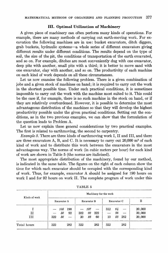
Example 3. There are three kinds of earthmoving work I, II and III, and there are three excavators A, B, and C. It is necessary to carry out 20,000 m3 of each kind of work and to distribute this work between the excavators in the most advantageous way. The norms of work (in cubic meters per hour) for each kind of work are shown in Table 5 (the norms are italicized).
The most appropriate distribution of the machinery, found by our method, is indicated in the same table. The figures on the right of each column show the time for which each excavator should be occupied with the corresponding kind of work. Thus, for example, excavator A should be assigned for 190 hours on work I and for 92 hours on work II. The complete program of work under this
TABLE 5
Machinery for the work Kinds of work
Excavator A Excavator B Excavator C 2
I - 105 190 - 107 - 312 64 20,000 II 56 92 302 66 222 38 - 20,000
III 322 56 20 83 60 10 53 282 20,000
Total hours 322 282 322 282 322 282

378 L. V. KANTOROVICH
TABLE 66
Equipment Kind of work 2 2 X 5.65
Pendulum saws (2) Circular saw (1) Disc saws (10) Frame saws (20)
I 400 X 2 167 X 3 59 X 9 1830 10,000 II 213 X 0 125 X 7 38 X 0 875 5,000
III 475 X 1 52 X 0 23 X 11 725 4,000
distribution can be achieved in 282 hours of work if the norms are fulfilled. For comparison in each case, the left side of the column gives an alternative "un- successful" pattern of distributing the excavators. With this distribution, under the same conditions, the indicated work will be completed in 322 hours; that is, the excess time (and the associated amounts of fuel, money, and so on) will amount to 14 per cent compared to the first which is the optimum variant. Let us note that even under the second variant the norms are fulfilled, the work goes forward without interruption and the machines are fully occupied. Therefore its shortcomings could not be revealed by any of the usual indicators, but only by specially directing attention to the question of a better distribution of the ma- chines.
Example 4. We have the following kinds of work: 1) cross-cutting of boards 4.5 m, 2 X 14-10,000 cuts; 2) cross-cutting of boards 6.5 m, 4 X 30- 5,000 cuts; 3) ripping of boards 2 m, 4 X 15- 4,000 running meters. The following machines are available: 1) pendulum saws 2; 2) circular saws with hand control 1; 3) electric disc saws 10; 4) frame saws 20. The norms of output (in number of cuts and running meters per hour) are
shown in Table 6. The same table shows the optimum distribution of the work. In Table 6 the first figure in each column shows the norm of the machine for
the corresponding kind of material (in number of cuts or running meters per hour). The multiplier given with each norm shows the number of machines oc- cupied with the corresponding kind of work; in particular, a multiplier of 0 shows that the given kind of equipment is not used on the corresponding work. All the work can be finished in 5.65 hours under this optimum distribution.
Let us note that it is possible to distribute the machinery not among kinds of work, but among separate tasks; that is, having listed the necessary tasks, and having defined the time required for each machine to perform each of them (including also set-up time), we can distribute the tasks among the machines so that they will be finished in the shortest time or within a given time but with the least cost.
6 The output norms are taken from the book Uniform Norms of Output and Valuations for Construction Work, 1939, Section 6, Carpentry.
MATHEMATICAL METHODS OF ORGANIZING AND PLANNING PRODUCTION 379
Other variants are possible in the stating of the problems; for example, to complete a given combination of jobs by a given date with the machines avail- able and with the least expenditure of electric energy.
The same questions of distribution of machinery can also be resolved when, for example, the machines require electrical energy and we are constrained by the condition that the capacity used should not exceed a certain amount; or the number of persons working may be limited; or the daily consumption of water is limited (for hydraulic methods of earthmoving), and so on. These ques- tions lead to Problem B.
The same methods can be applied to those problems not concerned with the utilization of existing machines, but with the selection of the most suitable ones for a given combination of jobs.
We believe that this method can be applied to other branches of industry as well as to earthmoving and other kinds of construction work.
In the fuel mining industry, coal-cutting machines of different systems under different conditions develop different productivities depending on the size of the vein, the conditions of transportation and so on. The most suitable distribu- tion of the stock of machines can result in a definite effect here.
The mining of peat is possible by various methods which have different ef- ficiencies for different kinds of peat. Therefore, there is the problem of distribut- ing the available machines among the peat fields with the aim of getting the maximum output. This problem can also be solved by our methods.
Moreover, in agriculture, various kinds of work can be performed by combines, threshing machines, binders, while certain machines (for example, combines) perform a whole range of operations. In this case the question of the distribution of agricultural machinery leads to Problem C.
IV. Minimization of Scrap
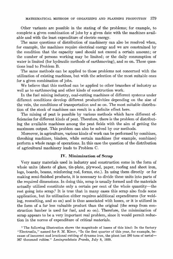
Very many materials used in industry and construction come in the form of whole units (sheets of glass, tin-plate, plywood, paper, roofing and sheet iron, logs, boards, beams, reinforcing rod, forms, etc.). In using them directly or for making semi-finished products, it is necessary to divide these units into parts of the required dimensions. In doing this, scrap is usually formed and the materials actually utilized constitute only a certain per cent of the whole quantity-the rest going into scrap.7 It is true that in many cases this scrap also finds some application, but its utilization either requires additional expenditures (for weld- ing, resmelting, and so on) and is thus associated with losses, or it is utilized in the form of a far less valuable product than the original (the scrap from con- struction lumber is used for fuel, and so on). Therefore, the minimization of scrap appears to be a very important real problem, since it would permit reduc- tion in the norms of expenditure of critical materials.
7The following illustration shows the magnitude of losses of this kind: In the factory "Electrosila," named for S. M. Kirov, "In the first quarter of this year, for example, be- cause of incorrect and irrational cutting of dynamo iron, the plant lost 580 tons of metal- 367 thousand rubles." Leningradskaia Pravda, July 8, 1939.
380 L. V. KANTOROVICH
Our methods can be applied here as follows. Let there be one or several lots of materials from which it is necessary to prepare parts of a given size; at the same time, the number of units of each part must fit a given set of ratios pi, P2 ,
p.., Pm. It is necessary to get the largest output (for example, from a given lot of sheets of glass of a standard size it is required to prepare the largest pos- sible number of sets of window panes). At the same time, let there be several ways of dividing up each unit into parts so it becomes necessary to select the number of units of each lot to which each method should be applied in order to minimize the amount of scrap. We shall show that this problem is solved by our methods since it leads to Problem C.
Let there by n lots of the material with the i-th lot consisting of qi parts. Let it be required to prepare the largest piossible number of sets of m parts each with the condition that there are in each set pi units of the first part, p *, pm units of the m-th part.
There are several possible methods for cutting a unit of each lot. Let us assume that under the l-th method of cutting a unit of the i-th lot, we get ai,k,l units of the k-th part (ai,i,z of the first part, ai,2,1 of the second part, and so on). Then, if we designate by hi,1 the number of units of the i-th lot which are to be cut by the l-th method, we have the following conditions for the determination of the un- knowns hi, :
1) hi l?> 0, and equal to whole numbers; 2) Ez hi,=qi;
E aei,,,, hij l a i,2,1 hill EaO!,nj hij 3) i, il = i,l
Pi P2 Pm
and that their common value be a maximum. It is clear that, with simple changes of expressions, this problem can be re-
duced to Problem C. We will illustrate the general discussion presented so far by an example relat-
ing to a very simple problem of units of linear dimensions. Example 5. It is necessary to prepare 100 sets of form boards of lengths 2.9,
2.1, and 1.5 meters from pieces 7.4 meters long. The simplest method would be to cut from each piece a set consisting of 7.4
-2.9 + 2.1 + 1.5 + 0.9 and then throw away the ends, i.e., the pieces 0.9 meters long, as scrap. This method would require 100 pieces, and the scrap would amount to 0.9 X 100 = 90 meters.
Now let us indicate the optimum solution. Let us consider the different meth- ods for cutting a piece of 7.4 meters into parts of the indicated lengths: these methods are shown in Table 7.
These methods include one by which no scrap at all is formed, but it is im- possible to use this method entirely since we would not obtain the required pro- portions (for example, no 2.1 meter parts would be produced).
The solution which gives the minimum scrap, found by our method, would be the following: 30 pieces by the first method; 10 by the second; 50 by the

MATHEMATICAL METHODS OF ORGANIZING AND PLANNING PRODUCTION 381
TABLE 7
I II III IV V VI
2.9 2.9 2.1 2.9 1.5 2.9 1.5 2.9 2.1 2.1 1.5 2.1 1.5 1.5 1.5 2.1 1.5 1.5 1.5 1.5 2.1
7.4 7.3 7.2 7.1 6.6 6.5
fourth. Altogether this requires only 90 pieces instead of the 100 needed for the simplest method. The scrap amounts to only (10 X .1) + (50 X .3) = 16 m; that is, 16:666 or 2.4 per cent. In any case, this is the minimum that can be obtained under the given conditions.
Let us examine another variant of this same problem with several modifica- tions of the conditions.
Example 6. There are 100 pieces 7.4 m in length and 50 pieces 6.4 m in length; it is required to prepare from them the largest possible number of sets of the previous dimensions 2.9, 2.1, and 1.5 m. The methods of cutting the 7.4 m pieces are given above. The 6.4 m pieces can be cut as follows: I) 2.1 + 2.1 + 2.1 = 6.3; II) 1.5 + 1.5 + 1.5 + 1.5 = 6.0; III) 1.5 + 1.5 + 2.9 = 5.9; IV) 2.9 + 2.9 = 5.8 and so on. The solution of the problem is to cut the 7.4 m pieces as follows: 33 by method I, 61 by method II, 5 by method IV, one by method VI and to cut all the 6.4 m pieces by the first method.
Altogether we get 161 sets, and the scrap consists of (61 X .1) + (5 X .3) + (1 X .9) + (50 X .1) = 13.5; 13.5: 1060 = 1.3 per cent.
It should be noted by the way that, usually, the more complicated the problem, the greater the possibilities of variation, and therefore it is possible by our method to achieve smaller amounts of scrap.
An analogous solution can also be obtained for other problems. I believe that, in a number of cases, such a mathematical solution to the prob-
lem of minimizing scrap could achieve an increase in the actual utilization of materials by 5 to 10 per cent over that obtained in practice. In view of the scar- city of all these materials (form lumber, processed timber, sheet iron, and so on), such a result would be significant and it is worthwhile for the engineer to spend a couple of hours to find the best methods of cutting lumber, and not to leave this matter entirely to the workers.
I also want to direct attention to the possibility of applying this method in the timber industry. Here it is necessary to minimize the scrap in cutting tree trunks into logs of given dimensions, into boards, and so on, since the amount of scrap in this case is extremely large. Large amounts of scrap are inevitable, it is true; nevertheless, it seems to me that if one resolves this question mathe- matically and works out rules for choosing sawing methods for logs of different sizes, this scrap can be significantly reduced. Then with the same type and quan- tity of raw material, these timber enterprises will provide more output.
382 L. V. KANTOROVICH
Of course this case is more complicated. In addition to the considerations already taken into account above, special work will be required to adapt this method to the given problems. But the possibility of applying it to this problem seems to me to be beyond doubt.
V. Maximum Utilization of a Complex Raw Material
If we consider a process like oil refining, there is a variety of products; gasoline, naphtha, kerosene, fuel oil, and so on. Moreover, for a given crude oil it is pos- sible to use several cracking processes to break up the component parts of the crude. Depending on which cracking process is used for a given crude, there will be a different output of these component parts. If the given petroleum enterprise has a definite plan, and uses one or several crudes as raw material, it should divide them among cracking processes in such a way as to obtain the maximum production of the required product mix. It is easy to satisfy oneself that the solution of this problem leads to Problem C.
I assume that there is no need to introduce the corresponding expressions again-this is done by the method used in the other problems. I have mentioned oil as an example, but the same conditions apply in using different kinds of coal and ores for the production of different kinds or qualities of steel. Here the selec- tion of the most suitable ore and coal and their distribution among different kinds of steel production gives rise to the identical problem.
We have the same problems in refining poly-metallic ores and in the chemical and coke-chemical industries; that is, where ever a given raw material can serve as the source of several kinds of products.
VI. Most Rational Utilization of Fuel
Different kinds of fuel such as oil, bituminous coal, brown coal, firewood, peat and shale can be burned to serve as the energy input to various kinds of installations, and give different efficiencies. They are used in the boilers of generating stations, locomotives, steamships and small steam machines, for steam-heating cities, and so on. At present, fuel is often allocated in a random way and not according to which kinds of fuel are most suitable for the given installation, or even whether a given kind of fuel can be used in a given installa- tion.
At the same time, the relative efficiency of fuels varies in different situations. For example, it is possible that in electric power stations two tons of brown coal equal one ton of anthracite while in locomotives, brown coal is considerably more difficult to utilize effectively and it is possible that only with 3 tons of brown coal will it be possible to obtain the same result as with 1 ton of anthra- cite. I suggest this only as an example, but such differences undoubtedly occur in practice.
The same applies also to different sorts of bituminous coal. Depending on the ash content, the size and other factors, the possibility and efficiency of combus- tion is different in different boilers.
Here again the most suitable allocation of fuel from the point of view of giving

MATHEMATICAL METHODS OF ORGANIZING AND PLANNING PRODUCTION 383
the highest percentage utilization of all installations on the basis of a given supply or its planned annual output can be decided by our methods and is equivalent to Problem A.
Another more complicated problem is based on a given plan of deliveries or output of fuel and is to choose the types of engines, (diesels, gas-generator in- stallations, steam turbines of various systems) and their percentage distribution such that they will utilize the given fuel and will give the maximum effect in terms of their output (in ton-kilometers in the case of railroads and other kinds of transportation, in kilowatt hours for electric power stations). This question reduces to Problem C.
VII. Optimum Fulfillment of a Construction Plan with Given Con- struction Materials
Here we outline the possibilities of using our methods in questions of con- struction planning.
In the Eighteenth Congress of the Communist Party of the Soviet Union, it was mentioned that, while the plan for industry in the Second Five Year Plan was overfulfilled, the plan for construction was underfulfilled.8 It was therefore not possible to utilize a certain portion of the resources originally committed to construction. The main reasons were the unavailability of certain kinds of ma- terials, certain special skills in the labor force, and so on, which held up con- struction for a long time or which did not permit it to begin although the finan- cial resources were available. At the same time it seems to us that the existing system of planning construction does not provide for the maximum utilization of materials in short supply, and that it would be possible to achieve greater fulfillment of the plan by a more appropriate allocation of materials.
It is known that many structures, such as bridges, viaducts, industrial build- ings, schools, garages, and so forth, and their component parts, can be completed with different variants (reinforced concrete, bricks, large blocks, stone, and so on). Moreover, several of these variants are often equally possible and even approximately equal in performance. Under the existing procedure, the selection of a varialnt in such a case is made by the design organization separately for each structure; moreover, the choice is often made completely arbitrarily on the basis of some insignificant advantage of one variant over another. Nevertheless, the choice of variant is extremely important, since the quantity of different raw materials needed in its fabrication (cement, iron, brick, lime, and so on) varies according to the variant chosen, and other important factors also differ (the quantity of labor of different skills, the construction machinery, transportation, etc.).
Therefore, the method of selecting the variant of construction determines, to a significant degree, the quantities of materials and other factors necessary for carrying out the whole construction plan in a given region or of a given con- struction authority and so determines shortages and surpluses of different in-
8 Bol'shevik, 1939, No. 5-6, p. 96.

384 L. V. KANTOROVICH
TABLE 8
Limiting factors
List of projects Materials Labor Construc- Money ______- ____ - _____ -Force (by tion Ma- Transpor- Allotments
Cement Lime Brick Metal Lumber specialtbes) (ey types) (by item)
Bridge Variant I Variant II Variant III
School Variant I Variant II
Garage Variant I Variant II
puts. In our opinion, the choice among variants of construction should not be carried out haphazardly nor for each structure separately, but simultaneously for all the structures of a given region or construction authority in order to achieve the maximum correspondence between the requirements of each ma- terial or other factor and the expected supply of these resources. Such a pro- cedure, it seems to us, would considerably reduce the shortages in deficit ma- terials and would make possible the greater fulfillment of a construction plan.
The procedure which we have proposed for drawing up the construction plan is approximately as follows. The planning authorities should establish, for every structure, several (2-3) possible and best variants and, for these, make an approximate calculation of the necessary materials and other basic factors. In this way, the planning authority in the given region obtains data approximately like that in the following scheme (Table 8).
After this the planning authority makes a choice among the variants such that the inputs of the necessary materials and other factors are covered for the output planned for the given year, and such that this practicable plan of con- struction includes as much as possible of the indicated list (in order of impor- tance).
The problem of the choice of variants in these cases leads to Problem C with several additional conditions, and in any case presents a problem solvable by our method even in very complicated cases (100-200 structures). We shall not dwell here on the various details as for example on the financial settlements among the different organizations which pool their plans, materials and financial resources. All these questions can also be satisfactorily resolved.
VIII. Optimum Distribution of Arable Land
It is known that the difference in soil types, climatic conditions, and other factors makes for different suitability of different regions and different plots of

MATHEMATICAL METHODS OF ORGANIZING AND PLANNING PRODUCTION 385
land for different agricultural crops. The correct selection of a plan of sowing also plays a definite role. I will remind you of the speech of one of the delegates to the 18th Party Congress. He said that, in his province, barley grows much better in the northern regions and wheat in the southern regions. However, the agricultural section of the province planning commission divided up the acreage of all crops equally among the regions, and even if one region cannot grow barley well, it still has some barley assigned. Deciding the question of how to distribute it more suitably is however not so simple.
In order to substantiate this statement, I shall show how the question leads to the mathematical problem. Let there be n plots with areas ql, q2, *... qn,
and m crops, which according to the plan should be in the following relation- ship: PI, P2 1 ... 2 pm. Assume that on the i-th plot the expected yield of the k-th crop is equal toai,k -
Now it is necessary to determine how many hectares of the first plot (or first region) to plant with one crop, how many with another crop, and so on, in order to obtain the maximum harvest. Let us designate by hi,k the number of hectares of the i-th plot planted with the k-th crop. Then we can write the sum Ek=Z hi,k
- qi, equal to the total area of the i-th plot (hik, of course, must not be nega- tive). The number of centners of expected harvest of the k-th crop from all the areas will then be Zk- = E ai,khi,k , and it is necessary for us to select the numbers Zk such that they should be related as the given numbers z1 pi =Z2: P2 =
* = zm pm ; that is, so as to maintain the relations between crops as given in the plan and to obtain maximum ZkX the maximum output. This problem leads to Problem A. Indeed, if we replace hi,kqi with the new unknowns h *k, and if we make aik = (l/pkqi)ai,k , then for the magnitudes h k and a*k we have exactly the equations of Problem A.
We have considered the question of obtaining the maximum yield for the given year. If we pose the question of getting the maximum yield over a series of years and take into account the effect of rotation of crops on yields, then the question becomes more complicated and leads to Problem C. If part of the land is irrigated and on the i-th plot of ground, when sowed with the k-th crop, the norm of expenditure of water is Ci,k liters per second per hectare, then we get the additional condition i,k Ci,khik
-` C, if by C we designate the total capacity in liters per second of the source of irrigation. That is, we come to Problem B.
Finally, we have already shown in Section III that it is also possible to use our methods for the solution of the problem concerning the optimum distribution of agricultural equipment according to kinds of work.
It should be mentioned that, in applying the given methods to agriculture, a certain caution is necessary because here the data (expected yield) are provided in very approximate form and therefore, if they are given incorrectly, the solu- tion can also turn out to be incorrect. However, it seems to me that, even though in such cases the application of the principle of the best distribution on the basis of approximate data can give the wrong solution in individual cases (if these data are incorrect), in the mass, on the average, this principle will still give a positive effect.
386 L. V. KANTOROVICH
IX. Best Plan of Freight Shipments
Let us first examine the following question. A number of freights (oil, grain, machines and so on) can be transported from one point to another by various methods; by railroads, by steamship; there can be mixed methods, in part by railroad, in part by automobile transportation, and so oIn. Moreover, depending on the kind of freight, the method of loading, the suitability of the transporta- tion, and the efficiency of the different kinds of transportation is different. For example, it is particularly advantageous to carry oil by water transportation if oil tankers are available, and so on. The solution of the problem of the distribu- tion of a given freight flow over kinds of transportation, in order to complete the haulage plan in the shortest time, or within a given period with the least expendi- ture of fuel, is possible by our methods and leads to Problems A or C.
Let us mention still another problem of different character which, although it does not lead directly to questions A, B, and C, can still be solved by our methods. That is the choice of transportation routes.
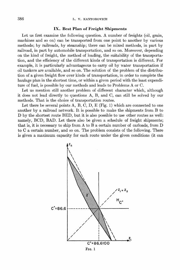
Let there be several points A, B, C, D, E (Fig. 1) which are connected to one another by a railroad network. It is possible to make the shipments from B to D by the shortest route BED, but it is also possible to use other routes as well: namely, BCD, BAD. Let there also be given a schedule of freight shipments; that is, it is necessary to ship from A to B a certain number of carloads, from D to C a certain number, and so on. The problem consists of the following. There is given a maximum capacity for each route under the given conditions (it can
z2
/Zg =: Z2
H C*
C*=86.6
C*=86.6100 FIG. 1

MATHEMATICAL METHODS OF ORGANIZING AND PLANNING PRODUCTION 387
of course change under new methods of operation in transportation). It is neces- sary to distribute the freight flows among the different routes in such a way as to complete the necessary shipments with a minimum expenditure of fuel, under the condition of minimizing the empty runs of freight cars and taking account of the maximum capacity of the routes. As was already shown, this problem can also be solved by our methods.
With this we conclude our examination of individual kinds of problems.
Conclusion
a) The general significance of the work
I see the basic significance of this work in the fact that it has developed a method of solving that kind of problem in which it is necessary to select the most advantageous from amongst a huge number of different cases and variants. Moreover, the given method makes the solution of the problem fully possible, often even in extremely complicated cases, where the selection of the most ad- vantageous variant must be made from among millions or even billions of con- ceivable possibilities. The method is also applicable where it is necessary to take various additional considerations into account.
It is generally known that this kind of question is constantly met in technical- economic problems, particularly in those dealing with the organization and planning of production. Many of these problems lead directly to Problems A, B and C, examined above, and therefore can be solved by our methods. Many other practical problems lead to mathematical problems which are different from these but can still be solved by the same methods.
Up to the present time all of these technical-economic problems have been solved more or less haphazardly by eye or by feel, and of course the solution obtained is only in rare cases the best. Moreover, the problem of finding the optimum has often never even been posed, and when it was posed it has not been possible in the majority of cases to solve it. The possibility now exists in a number of cases to obtain not an arbitrary solution but to find the optimum solution by a definite, scientifically based method.
b) The directions of further research
In its present form this work is far from finished, of course, and in a large de- gree does not meet the demands which are placed upon it. The given work is only a preliminary outline of a future thorough study on this theme in which it will be possible to clarify rather fully that important problem which up till now has for the most part only been posed. In order to achieve this, further extensive researches still have to be carried out by the combined efforts of mathematicians and production workers.
Much still remains to be done on the mathematical aspect itself, although an important step has been made: an extremely universal and rather effective method of solving a wide class of problems has been given. In the future it remains to determine the sphere of application of the method; to indicate further prob-

388 L. V. RANTOROVICH
lems solvable by it; to work out the details of the technique of applying the method,. to emphasize the distinctive features of this technique in different practical conditions; to work out simpler methods which will make it possible to find, if not the optimum solution, one extremely close to it and practically identi- cal with it; to improve the exposition of the method; and so on. Still more effort will be required to foster the actual utilization of this work by technicians and specialists in the different branches of the national economy.
Above all it is necessary to define those problems in different fields of the national economy where the applicability of our methods is most feasible and realistic. We have made some attempt to outline and indicate these questions in the present work, but of course it is difficult to expect them to be fully suc- cessful and not to evoke criticism on the part of specialists. It is possible that several of these problems will be shown to be unrealistic or unimportant, in others there will be essential corrections and additions. Finally, there is no doubt that a number of other problems, which have completely escaped our attention, will be raised.
Nevertheless, we considered it necessary to make such an attempt on the assumption that our methods would be more understandable and meaningful to an engineer if they were connected with concrete practical problems. And we pointed out a large number of such questions of divergent character to permit him to imagine better and to outline for himself the range of problems where our methods are applicable. He can also evolve and pose various similar problems in his own field; that is, he can facilitate the creative application of these methods.
After defining the fields in which the mathematical methods can be applied, the question will arise of the specifics of applying these methods to given ques- tions. This involves: a precise clarification of the circumstances under which these methods can give an appreciable effect and their application demonstrated; the working out of special technical data which are necessary for the application of these methods; the translation of these data into a form suitable for the utilization of tables; the working out of the details of the method specially for the problems met with in a given field (indication of a rule for the selection of a first approximation, for example, and so on.
c) Answer to several of the principal objections
As we have already indicated, we consider it probable that some of the exam- ples analyzed here (and possibly a whole field of questions) will encounter ob- jections on the part of specialists. We realize that in individual cases it is possible for these objections to be so wellfounded as to force our withdrawal from a certain field of application. However, along with these special individual objec- tions, we have been required to counter (in spite of the extremely favorable
9 Let us note that we do not expect it to be possible to go very far in perfecting the method; for example, to give solving formulae, tables or nomograms instead of the method of calculation which we have proposed. The trouble is that the setting of the problem in- volves a large number (up to forty) of different data, each moreover playing an individual r8le, and under these conditions a solution in the form of formulae or tables is unlikely.

MATHEMATICAL METHODS OF ORGANIZING AND PLANNING PRODUCTION 389
opinion of the majority) occasional objections of a general character which essentially lead to the denial, in principle, of the possibility of using mathemati- cal methods in technical-economic questions in the field of organization and planning. At this point I wish to examine these general objections.
The first consists of the following. In examining different practical concrete problems, the situation is so complex, there are so many circumstances to be considered, that it is impossible to take account of them all mathematically, or if you succeed in doing so then the equations obtained are still impossible to resolve.
We can make two remarks in reference to this. In the first place, as we have already shown, the indicated method is very powerful and flexible; that is, it obtains solutions in extremely complicated circumstances while taking account of a number of additional conditions; moreover, it permits different variations in using it (so that it is always possible to choose the most suitable method).
In the second place, if some practical detail has been left out of account, then after the optimum solution is found, it is possible to correct it with reference to this detail. This is all the more possible since the given method shows, along with the finding of the optimum solution, what variants give a solution close to the optimum so that there is the possibility of departing from the optimum solution only slightly in introducing the correction.
It should also be said that the objection noted could be equally justly raised to the use of any theoretical, and in particular mathematical, methods in techni- cal questions generally. It is well known how technicians value even the crudest theoretical representation of a phenomenon, for even that which considers just one of many factors involved is an extremely powerful guiding force in experi- ments, in calculations, and in designing. All the more valuable should be a method which allows a whole range of considerations to be taken into account in complicated situations.
The second objection is that, in using the method, it is necessary to have a whole series of data (ai,k in Problem A, and so on); but such data may not be available, and then we cannot use the method.
The answer is that the data which are needed (output norms on different machines and pieces of equipment, the quantity of different materials and their characteristics, and so on) are necessary for many other purposes such as for norm setting, wage calculations, norms for the expenditure of materials, reports and so on, and should exist in any normally working enterprise. In short, they are just as necessary for making any kind of plan as for making the best plan by our methods, and therefore the enterprise ought to have these data at its disposal.
In several cases it still turns out that such data are lacking; for example, some material is supposed to arrive at the construction project, it is not known just what kind, but in any case it must that very day be put to use. Or materials are sent which are different from those planned, and so on. Of course in those few enterprises where such primitive mismanagement reigns, no planning, even the most suitable, is possible. But if the desire to use our methods serves as an
390 L. V. KANTOROVICH
added stimulus for the elimination of such negligence, then this is only another argument in favor of this method.
The third objection is that the original data in a number of cases are doubtful and known only approximately (for example, the yields of different crops, the expenditure of water on hydro-mechanical working of earth, and other data in several of the examples introduced above) and therefore a calculation based on these data may be incorrect.
Here it is necessary to say first of all that in individual cases the optimum variant of a plan found by our method may indeed not be the optimum one because of the inaccuracy of the data.
However, we suppose that in the mass application the choice of the most advantageous variants, even with such doubtful data, will give, thanks to the statistical effect, an effective result. Let us clarify this by the following simple example. If we take the larger of two eggs, such a solution may be unfortunate: the egg may turn out to be rotten. But if out of a box of 1,000 eggs we choose the 500 largest, it is completely improbable that this choice would turn out to be wrong.
The fourth objection is that the effect of changing from the ordinarily chosen variant to the optimum one is comparatively small, in many cases only about 4-5 percent.
Here it is necessary in the first place to say that the use of the best method does not demand any additional expenditures in comparison with the usual one, except the absolutely insignificant expenditures on calculation. In the second place, the use of the method can be expected not in a single isolated problem, but in many; it is possible that it can be used even over the greater part of the branches of the national economy, and in that case not just one percent, but even each tenth of a percent is associated with tremendous sums.
The fifth objection is that, in a number of cases, the use of the method is im- possible as a result of various obstacles of an organizational character connected with the accepted procedure for approving plans, estimates, and so on. For example, if this or that material or mechanism is already distributed in a certain way between enterprises, then this distribution can not be changed during the interval of the given quarter, and so on.
This objection, of course, is not essential. If it is generally recognized that the use of the most effective plan results in a significant national economic effect, but that its introduction requires certain changes in procedure, then there is no doubt that such changes will be made.
Appendix I
Method of Resolving Multipliers
Here we intend to give a detailed exposition of the method of resolving mul- tipliers discussed in Section I, and which in our opinion is most effective for the solution of Problems A, B, and C as well as for many other problems of an analogous character connected with the choice of the most advantageous variant from among a very large number of possible ones. We shall examine chiefly the

MATHEMATICAL METHODS OF ORGANIZING AND PLANNIG PRODUCTION 391
use of this method in the basic problem, Problem A, although further on we shall discuss the other problems as well.
1. Solution of Problem A for m = 2. The general concept of the method
Let us first examine Problem A for the simplest case, when m = 2 (two parts). In this case the problem takes the form: find the numbers hi,1 and hi,2 satisfying the conditions:
1) hi, ; hi,2 _ 0;
2) hi,1 + hi,2 = 1; 3) EZ,1 ai,1hi,j = Ei71 ai,2hi,2
and their common value z has maximum possible value. Let us examine the relationship ai,2/ai,j = ki for all i (the ratios of the pro-
ductivity of each machine for parts I and II). Thus, on the first machine, a unit of part I is equal to ki units of part II, and so on. We may consider that the ratios k1, k2, * . , are arranged in order of increasing magnitude k1 ? k2 ?< * - .
If that were not so, we could make it so by changing the numbering of the machines. We could arrange these ratios in order of increasing magnitude and then call that machine the first on which the ratio was the smallest, and so on. Thus, we consider that the inequalities ki ? k2 < ... are satisfied.
It is clear that it is relatively more advantageous to produce part I on the first machine since the removal of one part from this machine would permit us to substitute for it only ki units of part II; whereas at the same time on all the others the corresponding numbers k2, k3, . * *, are greater than ki . On the second machine, it is less advantageous to produce part I than on the first machine but more advantageous than on all the rest of the machines. Therefore it is under- standable that the first machines should be assigned part I and the rest part II; that is, in the first cases it is necessary to make hi,1 = 1 and hi,2 = 0, and in the latter, hijl = 0 and hi,2 = 1. At the same time the total output of both parts must be identical. Proceeding from this condition, let us select a number s, such that
8-1 n
aZi < Z ai,2
s %n
Eai,l > a ?i,2; i i=8+1
this means that to assign (s- 1) machines to part I is too few (the output of part II will be greater), but to assign s will be enough or too many. Then it is clear that taking hi,1 = 1, hi,2 =0 for i = 1, 2, ... , s - 1; hi,1 = 0, hi,2 = 1 for i = s + 1, * * , n; and determining h8,1 and h8,2 on the basis of the conditions
hs,l + hs,2 = 1,
s-1 n
E ai-I + hs,1 jx,1 = Z ai,2 + h8,2 a8,2
webtantesluion tooui8+1 we obtain the solution to our problem.

392 L. V. KANTOROVICH
TABLE 1
Groups of machines Part
Milling Lathe Automatic
I 30 60 30 II 60 90 80
Let us apply this process of solution to our first example. The productivity of different groups of machines there is shown in Table 1.
80= 9 0=-3 80=8 Our ratios are 6 2, = -,~ 7, or in order of increasing magnitude: < 2 < ..Arranging the productivity figures in the same order (lathe, auto-
matic, milling), we get the following values for ai,k
aij = 60, a2,1 = 30, a3,1 = 30, axl,2 = 90, aX2,2 = 60, 2 a3,2 = 80.
Taking s = 2, we obtain
_a,ij = a,,= 60 < Z i, = aX2,2 + a3,2 = 140;
a ~~~~~~~~~n aj= a,,, *+ a2,1 = 90 > ~jai,2 = a3,2 = 80.
Consequently, hi,1 = 1, hi,2 = 0, h3,1 = 0, and h3,2 = 1. For the determination of h2,1 and h2,2 we have the equations
h2,1 + h2,2 =1
60 + 30h2,1 = 80 + 60h2,2,
from which h2,1 = and h2,2 = which also leads to that optimum distribution of the parts among machines which was given in Table 2 of Section I.
We now direct attention to a feature of the indicated process of solution which permits a way of extending this method from the simplest case where m = 2 to the case where m may be any number. We direct attention to the fact that a complete finding of the solution is entirely equivalent to finding the ratio k, corresponding to that s for which we are making a choice. Actually, if this ratio k. = a.9,2/as,i = X1/X2 (it will be more convenient to designate it thus in the future) is known, then the entire solution is found immediately. For those i's for which ai,2/ai,l < X1/X2 , or what is the same thing Xia,ij > X2ai,2, it iS necessary to give preference to part I; that is, take hi,1 = 1 and hi,2 = 0. For those where X2ai,2 > Xii give the preference to part 11; that is, take hi,1 = 0 and hi,2 = 1. And finally, for those i's where X2ai,2 =X1a,ij, the corresponadinag h is selected on the basis of the equation Za,ij hi,1 =Zai,2 hi,2 . This resolving ratio is the index of equilibrium which is established in the maximal distribution between two parts. In our particular example this equilibrium is established on the milling machine and X1/X2 f ~. It should be said that this resolving ratio is
MATHEMATICAL METHODS OF ORGANIZING AND PLANNING PRODUCTION 393
defined by the totality of the conditions of the problem; for example, it cannot be expressed only by ki, k2, ... . Actually, if in our particular example there were not one automatic machine but two, then for the optimum distribution it would be necessary to assign to Part I not only the lathe and the milling machine entirely, but also in part the automatic machine. The resolving ratio would then become X1/X2 = &. On the other hand, if the number of lathes were tripled, this ratio would become equal to -.
We shall use just this concept of resolving ratios for finding a method of solu- tion suitable for any m. In this case there naturally arises the thought that in- stead of finding the many ht,k, to try to find the ratios Xi, X2, * . , Xm (the indices of equilibrium under the optimum distribution). On the basis of these just as in the problem where m = 2 we could immediately indicate those hi,k
which it is necessary to take equal to zero. As a matter of fact, this method can actually be carried out. A detailed exposition of it is given below. Before taking it up, however, let us consider another auxiliary circumstance.
2. A transformation of Condition 3) of Problem A
For the purposes of what follows, it is important for us to show that it is possible to find another formulation of Condition 3) of Problem A equivalent to the original formulation.
Let us recall the formulation of Problem A. Problem A. The numbers ai,k > 0(i = 1, 2, ..., n; k = 1, 2,* ., m) are
given, and it is required to find hi,k which satisfy the conditions
1) hi,k 0;
2) EZ-1 hi,k = 1(i = 1, 2, n); 3) if we introduce the notation
Zk = 7=i a,khi,k,
then zi = Z2= = Zm, and their common value, z, has maximum possible value.
In making up the conditions which the hi,k must satisfy, we could reason some- what differently than we did in Section I of the text. Since the number of whole complexes is determined by the number of that part which we have least of (that is, by the smallest of the Zk) it equals z' = min (zl, Z2 , Zm). This number z' must also be a maximum.
In this way we arrive at Problem A'. Problem A'. Conditions 1) and 2) are the same as in Problem A, but instead
of Condition 3): 3') The quantity z' = min (zl , Z2 , Zm) has maximum possible value. Let us now show the equivalence of Problems A and A'; more precisely, let us
establish the following assertion. Theorem. If we designate by C the maximum value of z in Problem A, and
by C' the maximum value of z' in Problem A', then C = C' and if a certain system of numbers {hi,k} yields a maximum in Problem A, it will also give a maximum in Problem A'. Conversely, if a certain system of numbers {h'Z,k}
394 L. V. KANTOROVICH
gives a maximum in Problem A', from it we can easily obtain a system of num- bers { hi,k} which gives a maximum in Problem A.
Proof. Let the system of numbers hi,k give a maximum in Problem A; that is, for them we obtain zi = Z2 * * = Zm = C. For this same system we obviously have z'=min (zl, Z2 , * * * , Zm)=min (C, C, * *, C) = C.
Since C is that value which we obtained for z' under a certain selection of hi,k and C' is the maximum z' for all possible selections, then
C < C'.
For the proof of the reverse inequality, let us look once more at the basic case when all ai,k >0. Assume that we have z' = min (Zl , Z2 , * Zm) C' for a certain system { h'i ,k I. We assert that in this case necessarily all Zk = C'. As a matter of fact, assume on the contrary that one of them is greater than C', say z1 > C'. In this case it would be possible slightly to decrease all the h'i,,k at the expense of slight increase of the other hi,k,. Then as before we would still have z1 > C and all Z2 , * * * , Zm would also increase and would also become greater than C'. But then it would turn out that for this new system, z' = min (Zl , Z2 , * Zm) > C, and that contradicts the fact that C' is the maximum possible value for z'. Thus, necessarily z1 =Z2 = * = Zm = C'. Consequently, h,ik gives a system of values for which z1 = Z2 = * = Zm and their common value z is equal to C'; since C is the maximum possible value for z, necessarily
C' < C.
This inequality together with the previous one gives C' = C. We established the second inequality C' < C for the case where all a?,k > 0;
if certain ai,k = 0, then this inequality is also valid, but its proof requires several additional considerations which we shall not cite here.
3. The basis of the method of resolving multipliers.
We shall now show that the solution of Problem A, requiring the finding of a system of n m numbers hi,k, can be replaced by a problem of finding alto- gether only m numbers 'X, X2 , * * * X Xm which are the resolving multipliers.
By resolving multipliers for problem A we mean a system of m numbers X1i X2, ... * Xm(Xk 0 and not all zero) such that if for each i we consider the products
Xiaij , X2ai,2 a*'*aXkai,k
and designate by ti the value of the largest and then set equal to zero those hi,k for which the corresponding product is not a maximum, i.e., X)kti,,k < ti, it is possible to determine the other hi,k from the conditions
1) hi,k > 0;
2) EkZ, hi,k = 1; 3) Z1 = Z2 = ... = Zm
Let us show first of all that finding the resolving multipliers actually gives the solution to Problem A. Let us assert that if the resolving multipliers

MATHEMATICAL METHODS OF ORGANIZING AND PLANNING PRODUCTION 395
X1 X2, ... * X.a are found and numbers h*,k are determined by the method indi- cated above, then the z = z* obtained with their help is the maximum possible value.
Indeed, for the system of numbers h*,k we have m \ ~ ~m m n n m
Xk Z= Z k = E Z k k h*k (Xk a ti,k)h i=l k*=1 k=1 i=l i=1 k-1
n m n
- :Et hsh *,k = Et;. i=1 k=1 i=l
(We could everywhere replace Xkai,k by ti since for those cases where Xkai,k < ti, there is the condition h*,k = 0.
Now let hi,k be another system of numbers for which z1 = Z2 = Zm = Z.
Then we have m \ ~n m n n xn
( Xk) Z = ZXk Zk = EXk E ai,k hi,k = E E (m k ai k)hi,k k=1 k=1 k=1 i=l i-1 k=1
n m
< Z h: t = Eti i=1 k=1 i
Combining this inequality with the previous one we obtain
( xk) Z < k Z k=1 k=1
or z _ z*.
This also shows that the value z* is the maximum possible value for z; that is, the numbers h*,,k determined with the help of the resolving multipliers actually give the solution to Problem A.10
Thus, the whole problem leads to the finding of the resolving multipliers. Let
10 In order to show the r6le played by the introduction of the resolving multipliers, I shall show in greater detail what the method of solving Problem A based on the general rules of analysis actually consists of. In Problem A there is discussed the finding of the maximum value (under several additional conditions) of z, which is a linear function of hi,k . It is known that, to find a maximum of a linear function in an interval, it is sufficient to compare its values at the ends and choose the larger of them. The same rule is preserved in finding a maximum of a linear function of many variables on a polyhedron-it is enough to compare its values on the vertices. If we translate this rule into the language of analysis, it means that in the given case it is necessary to choose a system from among (n + m - 1) numbers hi,k , to make the rest equal to zero, and to determine the chosen hi,k from the (n + rn - 1) equations 21k hi,k = 1; Zl = Z2 Zm ; and to compare the values of z obtained. In each trial it will be necessary to solve a system of a small number of equa- tions but the number of trials which it will be necessary to make is i=O (1)i+i C(m_+) C7t C7 (Co G 1; Cm = 0 if m > n); that is, if n = 3 and m = 3, there are 90 trials; for n =
mn = 4, there are 8272 trials. In the problem of the Plywood Trust, n = 8 and m = 5, and the number of trials is of the order of a billion. Thanks to the presence of the resolving multipliers, all the unnecessary systems are rejected and it is necessary to solve only a single one.
396 L. V. xANTOROVICH
us show a way to find them. Let us note first that if we take, instead of the re- solving multipliers, which we are looking for, an arbitrary set of numbers X1%, X2? *
... * -XM we can still try to act as though they were the resolving multipliers.
That is, we can consider the products X10a,i, , X20ai,2 , .* X m0Cai,m , and take hi,k= 0 for all those k for which the corresponding product does not have maxi- mum value. It is necessary to say, however, that in such an arbitrary selection it usually turns out that among the products there is a single maximum one since for a given i all the hi,k must be taken equal to zero with the exception of that one which is taken equal to 1.
In this way, under such an arbitrary selection of Xk, the hi,k are fully deter- mined and together with them the Zk Z1?, Z20, . . Zm0 obtain definite values. Of course, these values are not equal to each other and without changing Xk
it is impossible to make them equal. In what direction should Xk be changed? We know that the solution of the problem will be reached when min (Zi,
Z2 I. * Zm) achieves its maximum possible value. But this minimum is de- termined by the smallest of the numbers Zk. Assume that the smallest of the numbers zi0, Z2? * Zm? in the system obtained is a certain z8?. It is necessary to make it larger but it is clear that it will be increased if, while not changing the other Xk, we replace X8 with a larger number. Indeed then, in the majority of cases the product X8ai,8 will turn out to be the maximum in its row and there- fore hi,8 will be taken equal to unity; by the same token, ze will achieve a value larger than z8? and min (zl, Z2 z. . ) will, generally speaking, take on a value exceeding the previous one.
In this, strictly speaking, lies the principle of finding the resolving multipliers: namely to increase Zk by changing Xk and in this way gradually to move toward the necessary extreme value. Of course, several variations are possible. Instead of increasing the low ones among the Zk, it is possible to reduce the larger Zk
by decreasing the corresponding Xk. However, if these operations are carried out at random, with no system, then there is no certainty that we will ever finish; one Zk will be increased while, on the other hand, others may be decreased and we may never get any closer to the answer. Therefore in the given process it is better to follow a definite system of calculations which we shall now describe. For greater clarity we shall base this calculation on an example.
4. A sample scheme of calculation
Let us examine the solution of the problem of the optimum distribution of the work of the excavators (Example 3).
In order to complete the kind of work indicated in the shortest possible time, it is necessary to obtain that distribution of the excavators which will guarantee the maximum productivity per hour, under the constraint that all work should proceed equally. Then the assigned problem leads precisely to Problem A where the role of ai,k is played by the given productivities of the excavators. (Their values are repeated below in Table 2.) First of all, it is advantageous to select, as initial values for the Xk, Xko, values inversely proportional to the sums Ei ai,k Xko = P/Zi ai,k, where any number may be taken for P.
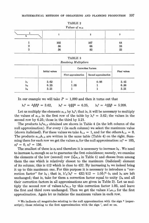
MATHEMATICAL METHODS OF ORGANIZING AND PLANNING PRODUCTION 397
TABLE 2 Values of aij,
k 1| t J 2 3
1 105 107 64 2 56 66 38 3 56 83 53
TABLE 3 Resolving Multipliers
Correction Factors Initial values Final values
First approximation Second approximation
3.62 1 0.98 3.45 X2 6.25 1.05 1 6.56 X3 5.21 1 1 5.21
In our example we will take P = 1,000 and then it turns out that
x? = 1,00 = 3.62, 2? =l = 6.25 x30 = 1 = 5.208.
Let us multiply the elements ai,k by Xko; that is, it will be necessary to multiply the values of ai,k in the first row of the table by X1? = 3.62; the values in the second row by 6.25; those in the third by 5.21.
The products Xk0ai,k obtained are shown in Table 4 (in the left column of the null approximation). For every i (in each column) we select the maximum value (shown italicized). For these values we take hi,k = 1, and for the others hi,k = 0. The products axi,khi,k are written in the same table (Table 4) on the right. Sum- ming them for each row we get the values Zk for the null approximation: Z1 = 105, Z2? = 0, Z30 = 136.
The smallest of these is Z2 and therefore it is necessary to increase X2 . We need to increase X2 enough so as to guarantee the first coincidence; namely, we examine the elements of the low (second) row (Xoai,k in Table 4) and choose from among them the one which is relatively closest to the maximum (italicized) element of its column; this is 412 which is close to 432. By increasing X2 we indeed bring it up to this maximum one. For this purpose it is necessary to introduce a "cor- rection factor" for X2 ; that is, X2/X20 = 432/412 = 1.05;11 . Xi and X2 are left unchanged; that is, take for them a correction factor equal to unity (Xk and all their correction factors in all approximations are given in Table 3). Let us mul- tiply the second row of values Xkoai,k by this correction factor 1.05, and leave the first and third rows unchanged. Then we get the values X'kai,k for the first approximation. Again let us italicize the maximum values in each row.
11 We indicate all magnitudes relating to the null approximation with the sign 0 (super- script); those relating to the first approximation with the sign ', and so on.
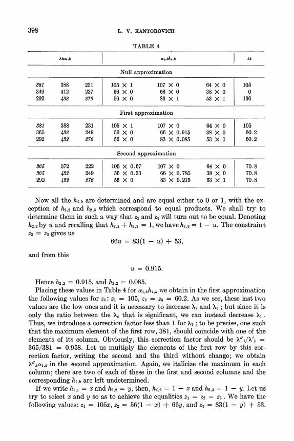
398 L. V. KANTOROVICH
TABLE 4
X xk aic ai,khiik zk
Null approximation
381 388 231 105 X 1 107 X 0 64 X 0 105 349 412 237 56 X 0 66 X 0 38 X 0 0 292 2 276 56 X 0 83 X 1 53 X 1 136
First approximation
381 388 231 105 X 1 107 X 0 64 X 0 105 365 432 249 56 X 0 66 X 0.915 38 X 0 60.2 292 432 276 56 X 0 83 X 0.085 53 X 1 60.2
Second approximation
365 372 222 105 X 0.67 107 X 0 64 X 0 70.8 365 432 249 56 X 0.33 66 X 0.785 38 X 0 70.8 292 482 276 56 X 0 83 X 0.215 53 X 1 70.8
Now all the hi,k are determined and are equal either to 0 or 1, with the ex- ception of h2,2 and h2,3 which correspond to equal products. We shall try to determine them in such a way that Z2 and z3 will turn out to be equal. Denoting h2,2 by u and recalling that h2,2 + h2,3 = 1, we have h2,3 = 1 - u. The constraint Z2 = Z3 gives us
66u = 83(1 - u) + 53,
and from this
u = 0.915.
Hence h2,2 = 0.915, and h2,3 = 0.085. Placing these values in Table 4 for ai,khi,k we obtain in the first approximation
the following values for Zk Zl = 105, Z2 = z3 = 60.2. As we see, these last two values are the low ones and it is necessary to increase X2 and X3 ; but since it is only the ratio between the Xk that is significant, we can instead decrease Xi. Thus, we introduce a correction factor less than 1 for Xi ; to be precise, one such that the maximum element of the first row, 381, should coincide with one of the elements of its column. Obviously, this correction factor should be X"1/X'1 =
365/381 = 0.958. Let us multiply the elements of the first row by this cor- rection factor, writing the second and the third without change; we obtain xi/kaj,k in the second approximation. Again, we italicize the maximum in each column; there are two of each of these in the first and second columns and the corresponding hi,k are left undetermined.
If we write hi,l = x and h2,2 = y, then, hi,2 = 1-x and h2,3 = 1-y. Let us try to select x and y so as to achieve the equalities z1 = Z2 = Z3. We have the followving values: z1 = 105x, Z2 = 56(1 - x) + 66y, and Z3 = 83(1 - y) + 53.

MATHEMATICAL METHODS OF ORGANIZING AND PLANNING PRODUCTION 399
Consequently, we obtain the equations
105x = 56(1- x) + 66y = 83(1- y) + 53 = z.
Hence, X = , y = %.6 _
Placing these expressions in the middle equation, we obtain for z the equation:
164.2 - 0.532z - 0.795z = z,
whence z = 70.8 and further, x = 0.67 and y = 0.785. The values x and y which we have found also give us the values hi,k for the
second approximation; at the same time, these turn out to be the solution to the problem.
The value which we have found for z, 70.8, shows the maximum output per hour on all three kinds of work under the condition that these outputs be equal.
Since it is required to carry out 20,000 m3 of work of each kind, then the mini- mum necessary time is 20,000/70.8 = 282 hours. Multiplying by 282 the values for hi,k, we get the amount of time that each machine should spend on each kind of work and which were indicated earlier (Section III, Table 5).
In this example we have shown the basic procedure for finding the solution. Now we shall make certain comments on carrying out this scheme.
5. Additional directions for the scheme
First of all, let us mention the following. Carrying out the scheme in the example introduced above was extremely simple; its realization in other cases might lead to additional difficulties which we shall now examine. Passing from the null approximation to the first, we increased the values of z2 and Z3 . In this way we succeeded, after having determined h2,2 and h2,3 in suitable form, to achieve the equality z2 = Z3. However, it will not always work this way. For the determination of u we had an equation from which we found u = 0.915. But generally this equation will have the form
a + bu = c(l - u) + d,
and its solution will not necessarily be achieved within the limits 0 and 1; but the latter condition, i.e., that 0 < u < 1, is absolutely essential to us. Let us note first of all that in any case we have a < c + d. (This inequality is equiva- lent to the fact that Z20 < Z30 since both parts of the above equation become Z20 and z3? when u = 0.) If we now have a + b > d, then the solution of the equation also satisfies the inequality 0 < u < 1. If it turns out that a + b < d, then the solution is greater than 1. In such a case it is necessary to take u = 1, since then although we do not achieve the equality Z2 = Z3, still we bring Z2
as close to Z3 as possible. The investigation of this case may also be carried out in another way as
follows. Since we are interested in the maximum increase of min (Z2, z3), then we must find the largest number t with which for some u(0 _ u _ 1) it is possible

400 L. V. KANTOROVICH
to satisfy both inequalities
a + bu > t, c(1-u) + d _ t.
Because of the first equation, we have
- b
and in addition u> 0; then the second inequality gives us
< c + d
t < d + c(l - u) t -a) b
Solving these two inequalities concerning t and choosing the smallest of the bounds obtained, we also obtain the largest t for which the original inequalities are solvable.
This last way of reasoning is suitable even for other cases when we obtain intersections not of two, but of several Zk .
Thus, in the case when we increase two equal values of Zk to a third, then (see the preceding example) the equations which are to be solved take the form
a + bx = c + dy = e(1 - x) +f(l - y) + g.
The solutions for x and y can turn out to be outside the limits of 0 and 1. Since we are interested most of all in obtaining the maximum of min (Zl, Z2, Z3), it is necessary again to find the maximum t for which it is possible to satisfy all the inequalities
a+bx > t, c+ddy _ t, e(1-x) + f(l-y) +g >t.
Hence, we have x _ (t -a) /b, y _ (t -a)/Ic,
and in addition x > 0, y ? 0. Then the third inequality gives us
0 1 _ t - a) +f (1 _ tc) +g
e +f( _ t-c++ g
et +f + 9
depending on which pair of the inequalities for x and y are utilized. Solving these inequalities concerning t and choosing the smallest of the values obtained, we also get the value of t sought which is the maximum for which all three of the primary inequalities can be satisfied. After t has been determined, the x and y

MATHEMATICAL METHODS OF ORGANIZING AND PLANNEING PRODUCTION 401
associated with it are found easily and the calculation of the given approxima- tion is finished. For going on to the next approximation, again we find among the Zk one or several of the smallest and increase the corresponding Xk .
Note that among the inequalities determining t it is actually necessary to use the first; that is, it gives the smallest value for t in the case when it is possible to satisfy the equations z1 = Z2 = Z3 . Let us also indicate that the argument given here for the case of dual and triple coincidences is, with slight modifications, also applicable to more complicated cases.
The exposition of the preceding section 4, together with the additional ex- planations included here, gives a fully determined "ironclad" solution scheme. It is necessary always to find the smallest (or the several smallest which are equal to each other) from among the numbers Zk and to increase them by the definite method described above. It is necessary to say that the literal following of this scheme can be recommended for simple cases (where n is small) and also for complex cases (where n is large) before the end of the solution when we are already sufficiently close to it (the Zk differing little among themselves). At the start of the calculation, it is expedient to depart from this scheme; for example, to increase not only the smallest but at the same time several of the small Zk,
and to reduce (by reducing Xk) the largest Zk, and in the process of the solution not to endeavor to obtain scrupulously equality between the smallest Zk (i.e. not to solve the intermediate systems). All these simplifications, which can often reduce the time of calculation, do not affect the essence of the solution; it is important to find the Xk, but the route to their discovery is not at issue.
In connection with this, it is useful to indicate that all the intermediate com- putations connected with determination of the Xk can be carried out with ex- tremely little precision to two or three places (on the slide rule). This will not affect the result. If a precise result is derived, then it is necessary to carry out with corresponding accuracy only the last calculation, which is the solution of the system from which the final values of the hi,k are determined. It is necessary to say only that if we are carrying out the calculations, for example, with a relative error of 0.01 then we can consider as identical two products Xkai,k differ- ing from each other by less than 0.01.
Finally, let us consider the following. The difficulty of solving the problem depends essentially on the values of n and m, and the solution gets more com- plicated particularly with an increase in m; for example, as we have seen for the case of m = 2, the solution is extremely simple for any n. Therefore, it is neces- sary to try to reduce n and m. Above all, if two rows of the ai,k in the table are proportional, for example ai,2 = kai,j for any i, then it is possible to introduce a new a' = aci(l + k) and substitute it for ail and ai,2 ; that is, n will be reduced by 1. This means for example that, instead of two machines the outputs of which are proportional, we introduce a fictitious new machine the output of which is equal to the aggregate outputs. Further, if we have m > n, then it is advan- tageous to reverse their roles; that is, instead of ai,k, to introduce ai,k = ak,i
but then to find not the maximum z but the minimum; that is, to find hi,k so that z1 = Z2 = . = Zn and that this value turns out to be a minimum. In

402 L. V. KANTOROVICH
practical language, this substitution means that instead of considering the problem to be one of getting the maximum output in a day, we are considering it as one of getting a given output in the shortest time; obviously, these two problems are equivalent to each other.
6. On checking the solution
In many mathematical problems there is no need to check the whole process of solution in order to check the accuracy of the solution obtained; one can judge directly by the result. For example, for checking the solution to an equation it is sufficient to substitute the obtained solution into the equation. For checking the correctness of a solution of Problem A also, it is sufficient to introduce only the final values Xk and the products Xkai,k and ai,khi,k for the last approximation and convince oneself that the hi,k which are larger than zero correspond to the underlined maximum Xkai,k and that the Zk are equal in value. If this is actually so, then the solution is found to be correct. The existence of such a check is useful in that the engineer or the economist can hand over the task of finding a solution to a special computational assistant; then he can check the solution in 10 or 15 minutes with no difficulty at all.
7. Concerning an approximate solution of Problem A
The solution of Problem A turns out to be rather lengthy and laborious when n and m are not small. Therefore, it is desirable to indicate simpler methods which would make it possible to find not an exact solution of the problem but one extremely close to it in effectiveness. Here we intend only to point out certain approaches for working out such methods.
First of all, let us note that, since a solution corresponds to the case where h ,k > 0 only for the pairs (i, k) corresponding to the maximum products Xkai,k,
we obtain an approximate solution if we allow hi,k different from zero for those (i, k) for which the products Xkai,k are close to the maximum. Therefore the first way for finding an approximate solution is as follows. In the tables of products Xkai,k in each column (with the exception of one) together with the maximum Xkai,k we underline the one closest to it (the one closest to it should not be under- lined in the case where it differs most, relatively that is, from its maximum). After this it is necessary to try to find the hi,k for the indicated (i, k) from the condition that Zk hi,k 1, and the equations z1 = Z2 = . = Zm . We recom- mend the reader to check for himself that the application of this method in the example of Section 4 will lead straightaway to the final solution.
The other way is based on another consideration. We have shown already in the previous section 6 that if two columns are
proportional they may be combined into a single one. In order to obtain an approximate solution, this assimilation can be used even where the propor- tionality is only approximate. Thus, combining the approximately similar ele- ments into groups, one can significantly decrease n and m and in the same way appreciably simplify the problem. The solution of this simplified problem will be, of course, only an approximation of that for the original one.
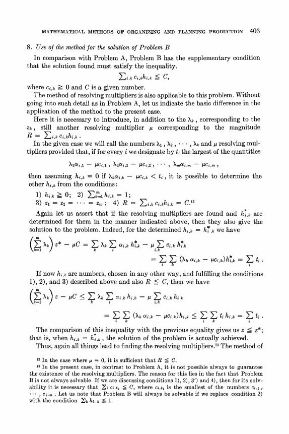
MATHEMATICAL METHODS OF ORGANIZING AND PLANNING PRODUCTION 403
8. Use of the method for the solution of Problem B
In comparison with Problem A, Problem B has the supplementary condition that the solution found must satisfy the inequality.
Ei,k Ci,khi,k < C,
where Ci,k _ 0 and C is a given number. The method of resolving multipliers is also applicable to this problem. Without
going into such detail as in Problem A, let us indicate the basic difference in the application of the method to the present case.
Here it is necessary to introduce, in addition to the Xk, corresponding to the Zk, still another resolving multiplier , corresponding to the magnitude R = Z,k Ci,khi,k -
In the given case we will call the numbers X1I, X2, X. *, Xk and , resolving mul- tipliers provided that, if for every i we designate by ti the largest of the quantities
Xlyij - WCi,l, X2ai,2 - ICi,2, ... * Xm0i,m - MCi,mX
then assuming hi,k = 0 if Xkai,k - UCi,k < ti, it is possible to determine the other hi,k from the conditions:
1) hi,k _ 0; 2) Z-l hi,k = 1;
3) Zl = Z2 = . = Zm; 4) R = Ei,k Ci,khi,k = C.12
Again let us assert that if the resolving multipliers are found and h*j,k are determined for them in the manner indicated above, then they also give the solution to the problem. Indeed, for the determined hi,k = ,k we have
^k) Z* -
UC = EAk Eaji,k h*k - A (Xk ,k -=
k=1 k i i,k
=E E: (Xk aix,k ,UCi ,k) sk =Eti
If now hi are numbers, chosen in any other way, and fulfilling the conditions 1), 2), and 3) described above and also R ? C, then we have
( Xk) Z - IC < Z Xk ai,khi,k A Ci,k hik k=1 k iZi,k
= E Z (xk ai,k -
/-ci,k)hi,k ? Z Z ti hi,k = Z ti. i k i k i
The comparison of this inequality with the previous equality gives us z < z*; that is, when hi,k = X, the solution of the problem is actually achieved.
Thus, again all things lead to finding the resolving multipliers."3 The method of
12 In the case where,u = 0, it is sufficient that R < C. 13 In the present case, in contrast to Problem A, it is not possible always to guarantee
the existence of the resolving multipliers. The reason for this lies in the fact that Problem B is not always solvable. If we are discussing conditions 1), 2), 3') and 4), then for its solv- ability it is necessary that Li Ciki <_ C, where Ci,ki iS the smallest of the numbers ci,i, ... ci,m . Let us note that Problem B will always be solvable if we replace condition 2) with the condition Lk hi, k < 1.

404 L. V. KANTOROVICH
TABLE 5 Ci .k
k 1 \ | t _ r 2 3
1 12 21 15 2 12 20 11 3 12 17 14
TABLE 6
Correction Factors Initial values Final values
I Approximation II Approximation III Approximation
Xi 3.62 1 0.973 1 3.53 X2 6.25 1.063 1 1 6.65 Xs 5.21 1 1 0.976 5.07
9 7.45 1 1 0.751 5.59
finding them is approximately the same as in Problem A. Without going into details here, let us illustrate these methods and the additional considerations needed by the solution of the following example.
Example. Let the table of ai,k be the same as shown in the example of Section 4 (Table 2). We will assign the values of Ci,k as shown in Table 5, and let C = 43. It is impossible to use the solution obtain earlier since the values for hi,k found there lead to the following: R = 12(0.67) + 12(0.33) + 20(0.785) + 17(0.215) + 141(1) = 45.4> 43.
As the initial null values Xk, let us take the same ones as before; as the initial value of ,u let us take, for example,
o 1000 1000 u0 - 134 = 7.45.
i,k
Let us compute for the given Xk0 and ;ii the Xkai,k - XCi,k (see Table 7) and in each column italicize the largest of the numbers obtained. We take the hi,k
corresponding to these largest numbers as unity and the others equal to 0. As we see, the one which is too low is Z2. Accidentally, R has turned out to equal C = 43.
Next, we must increase Z2.
The number closest to its maximum is 237 - 82. Let us increase X2, by pro- viding the factor E2, the value of which (in order to obtain a coincidence) is to be determined by the equation
237E2 - 82 = 276 - 105.
Whence, E2 = 253/237 = 1.063. Let us multiply the first elements of the second row by it and then italicize the maximum elements. It is necessary to de-
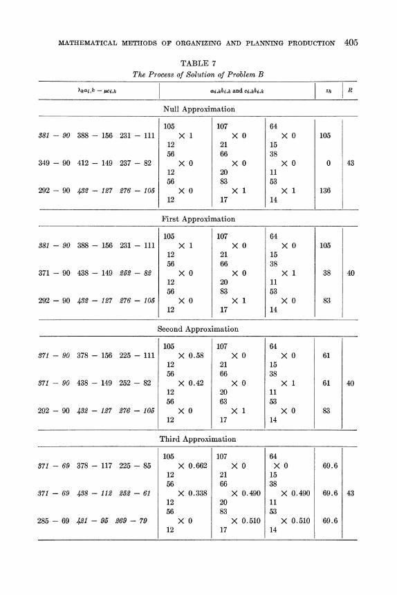
MATHEMATICAL METHODS OF ORGANIZING AND PLANNING PRODUCTION 405
TABLE 7 The Process of Solution of Problem B
Xka,,k -,uCi.k ai,khi,k and ci,khi,k Zk R
Null Approximation
105 107 64 381 - 90 388 - 156 231 - 111 X 1 X 0 X 0 105
12 21 15 56 66 38
349 - 90 412 - 149 237 - 82 X 0 X 0 X 0 0 43 12 20 11 56 83 53
292 - 90 432 - 127 276 - x05 X O X 1 X 1 136 12 17 14
First Approximation
105 107 64 381 - 90 388 - 156 231 - 111 X 1 X 0 X1 105
12 21 15 56 66 38
371 - 90 438 - 149 252 - 82 X 0 X 0 X 1 38 40 12 20 11 56 83 53
292 - 90 432 - 127 276 - 105 X O X 1 X O 83 12 17 14
Second Approximation
105 107 64 371 - 90 378 - 156 225 - 111 X 0.58 X 0 X 0 61
12 21 15 56 66 38
371 - 90 438 - 149 252 - 82 X 0.42 X 0 X 1 61 40 12 20 11 56 63 53
292 - 90 432 - 127 276 - 105 X 0 X 1 X 0 83 12 17 14
Third Approximation
105 107 64 371 - 69 378 - 117 225 - 85 X 0.662 X 0 X 0 69.6
12 21 15 56 66 38
371 - 69 438 - 11 2 252 - 61 X 0.338 X 0. 490 X 0.490 69.6 43 12 20 11 56 83 53
285 - 69 421 - 95 269 - 79 X O X 0.510 X 0.510 69.6 12 17 14

406 L. V. KANTOROVICH
termine h3,2 = u and h3,3 = 1-u. Since it is impossible to satisfy the equation Z2= 38u = 53(1 - u) + 83 = z3 for 0 _ u _< 1, it is necessary to bringZ2and Z3 as close together as possible. In order to do this, it is evidently necessary to take u = 1. Thus the first approximation is found. Here it turns out that R = 40. To proceed to the next approximation it is necessary to increase Z2, or alterna- tively to decrease z1. Again, for finding the correction factor El for X1, we write the equation 381e, - 90 = 371 - 90, from which El 0.973. This gives us the transition to the second approximation (we will not go through the minor com- putation associated with this). Now it is necessary to reduce Z3. Thus, we must provide X3 with an additional correction factor E3. On the other hand, R is not large enough (R < C) and so we must increase R; for this it is necessary to decrease ,u; we provide for it a correction factor 'y. The presence of two correction factors E3 and -y permits us to achieve these two coincidences. But in Problem B we have to have one more coincidence since for the determination of the re- maining hi,k we add the additional equality, R = C. Thus for the determination of E3 and Py we introduce the equations corresponding to the requirement of two coincidences,
438 - 149y = 432e3 - 127)y, 252- 82-y = 276e3 -105,
from which, E3 = 0.976, and -y = 0.751. After the introduction of these correction factors we pass to the third approximation. Now we have in each column one coincidence. Let us introduce the unknowns x, y, v:
hij =x; h1,2= 1-x; h2,2=y; h2,3= 1-y; h3,2=v; h3,3= 1-v.
The equations z1 = Z2 = Z3 = t and R = C can then be written
105x = 56(1- x) + 66y + 38v = 83(1 - y) + 53(1 - v) = t, 12x + 12(1-x) + 20y + 17(1-y) + llv + 14(1-v) = 43.
The last equation after simplification gives y = v and the first takes the form
105x = 56(1 - x) + 104y = 136(1- y) = t,
from which t = 69.6, x = 0.662, y = v =0.49.
This then finishes the calculation of the third approximation which coincides with the final solution of the problem. Note that the maximum output of the machines, which we have calculated under the additional constraint, turns out to be 69.6; that is, it is smaller than the 70.8 previously found for the earlier set of conditions.
9. Use of the method for solving Problem C
The difference between Problem C and Problem A consists in the fact that the Zk are determined in a more complicated manner, namely
Zk = Zi, Yi,k,jhj,j .
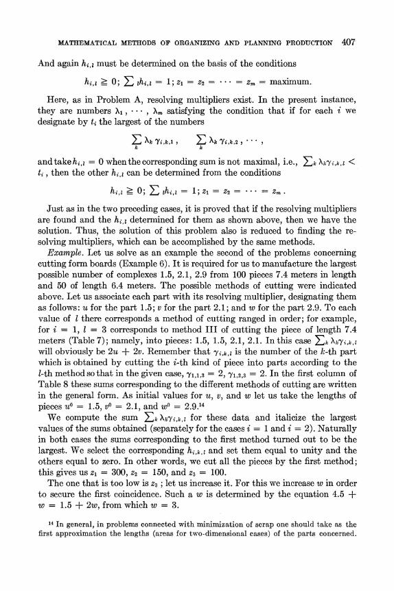
MATEIEMATICAL METHODS OF ORGANIZING AND PLANNING PRODUCTION 407
And again hi,, must be determined on the basis of the conditions
hi,0 > O; zhi,,z = 1; Zl = Z2= * ... = zm = maximum.
Here, as in Problem A, resolving multipliers exist. In the present instance, they are numbers X1, * **, X. satisfying the condition that if for each i we designate by ti the largest of the numbers
E kYi,k,l, 1 X k Pi,7c,2X***X k k
andtakehhi, = 0 whenthe corresponding sum is not maximal, i.e., Zk Xk7i,k,I <
t,, then the other hi can be determined from the conditions
hi? > 0; E ihij = 1; Z1 = Z2 = ... = Zm.
Just as in the two preceding cases, it is proved that if the resolving multipliers are found and the h, z determined for them as shown above, then we have the solution. Thus, the solution of this problem also is reduced to finding the re- solving multipliers, which can be accomplished by the same methods.
Example. Let us solve as an example the second of the problems concerning cutting form boards (Example 6). It is required for us to manufacture the largest possible number of complexes 1.5, 2.1, 2.9 from 100 pieces 7.4 meters in length and 50 of length 6.4 meters. The possible methods of cutting were indicated above. Let us associate each part with its resolving multiplier, designating them as follows: u for the part 1.5; v for the part 2.1; and w for the part 2.9. To each value of 1 there corresponds a method of cutting ranged in order; for example, for i = 1, 1 = 3 corresponds to method III of cutting the piece of length 7.4 meters (Table 7); namely, into pieces: 1.5, 1.5, 2.1, 2.1. In this case Zk XkYi,k,l
will obviously be 2u + 2v. Remember that 'Yi,k,l is the number of the k-th part which is obtained by cutting the i-th kind of piece into parts according to the l-th method so that in the given case, 'Y1,1,3 = 2, 'Y1,2,3 = 2. In the first column of Table 8 these sums corresponding to the different methods of cutting are written in the general form. As initial values for u, v, and w let us take the lengths of pieces u? = 1.5, vI = 2.1, and w? = 2.9.14
We compute the sum ZkXkYi,k,l for these data and italicize the largest values of the sums obtained (separately for the cases i = 1 and i = 2). Naturally in both cases the sums corresponding to the first method turned out to be the largest. We select the corresponding hi,k,l and set them equal to unity and the others equal to zero. In other words, we cut all the pieces by the first method; this gives us z1 = 300, Z2 = 150, and Z3 = 100.
The one that is too low is Z3 ; let us increase it. For this we increase w in order to secure the first coincidence. Such a w is determined by the equation 4.5 + w = 1.5 + 2w, from which w = 3.
14 In general, in problems connected with minimization of scrap one should take as the first approximation the lengths (areas for two-dimensional cases) of the parts concerned.
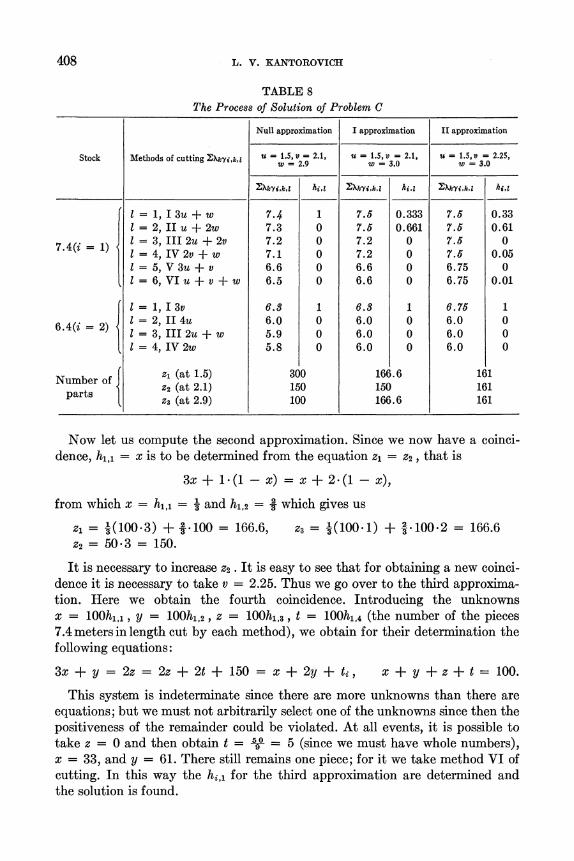
408 L. V. KANTOROVICH
TABLE 8 The Process of Solution of Problem C
Null approximation I approximation II approximation
Stock Methods of cutting Xki,bk,l u = 1.5, v = 2.1, u = 1.5, v= 2.1, u = 1.5, v = 2.25, 9 ~~w = 2.9 w =3.0 w =3.0
2XkYi,k,l hi,z 2XlkYi,kz t,l - y 2AkYi,k,l hi,z
{ l = 1, I13u + w 7.4 1 7.6 0.333 7.6 0.33 l = 2, II u + 2w 7.3 0 7.6 0.661 7.6 0.61
7.4(i =1) I = 3, III 2u + 2v 7.2 0 7.2 0 7.5 0 - = 4, IV 2v + w 7.1 0 7.2 0 7.6 0.05
I = 5, V 3u + v 6.6 0 6.6 0 6.75 0 1 = 6, VI u + v + w 6.5 0 6.6 0 6.75 0.01
I = 1, I 3v 6.3 1 6.3 1 6.76 1
6. 4(i 2) 1 = 2, II 4u 6.0 0 6.0 0 6.0 0 l = 3, III 2u + w 5.9 0 6.0 0 6.0 0 I = 4, IV 2w 5.8 0 6.0 0 6.0 0
Number of z1 (at 1.5) 300 166.6 161
parts z2 (at 2.1) 150 150 161 Z3 (at 2.9) 100 166.6 161
Now let us compute the second approximation. Since we now have a coinci- dence, h1il = x is to be determined from the equation z1 = Z2, that is
3x + 1 * (1 -x) = x + 2. (1 -x),
from which x = h = i and h1,2 = - which gives us
Z, = (100 * 3) + 2.1oo = 166.6, Z3 = '(100 * 1) + *100 *2 = 166.6 Z2= 50 3 = 150.
It is necessary to increase Z2. It is easy to see that for obtaining a new coinci- dence it is necessary to take v = 2.25. Thus we go over to the third approxima- tion. Here we obtain the fourth coincidence. Introducing the unknowns x = 100h1i , y = 100h1,2, z = 100h1,3, t = 100h1,4 (the number of the pieces 7.4 meters in length cut by each method), we obtain for their determination the following equations:
3x + y = 2z = 2z + 2t + 150 = x + 2y + ti, x + y + z + t = 100.
This system is indeterminate since there are more unknowns than there are equations; but we must not arbitrarily select one of the unknowns since then the positiveness of the remainder could be violated. At all events, it is possible to take z = 0 and then obtain t = v-5 (since we must have whole numbers), x = 33, and y = 61. There still remains one piece; for it we take method VI of cutting. In this way the hi,j for the third approximation are determined and the solution is found.

MATHEMATICAL METHODS OF ORGANIZING AND PLANNING PRODUCTION 409
10. Direct application of resolving multipliers
Thus far we have considered the resolving multipliers only as a technical means for the solution of Problems A, B, and C; they found application only in this way. Thus it could appear that the method of solving Problems A, B, and C based on the resolving multipliers has no particular advantage over other possible methods, apart from say its simplicity or brevity. However, that is not the case; the resolving multipliers have a far greater significance. They not only give the solution to the problem, but they also make it possible to indicate a number of characteristics of the solution that are important in its application. Thus the solution obtained by the resolving multipliers gives far more than the bare result, the numerical values of the hi,k . Here we want to turn our attention to these applications of the method of solution itself.
The quantities Xk and ti determined above in the process of solution can be exploited in a whole series of questions connected with the application of the maximal solution. For concreteness, I shall relate all these comments to the first interpretation of Problem A which concerns the production of a set of parts. In this case the multipliers Xk are indices of equivalence for different parts under the maximal solution. Thus, the production of X. of the k-th part is equivalent to the production of Xk of the s-th part. The production of 100 units of the k-th part is equivalent to the production of 100 (Xk/E Xk) units of the manufactured item. Thanks to this, if one sets up as the problem, for example, not the produc- tion of z = Zl = Z2 = * = Zm pieces of complete sets which are possible during a day, but (z + Az,) units of the first part, (z + AZ2) of the second, and so on (Az, not too large), then it is possible to indicate the time which this task will require for its completion, namely
Z Xk AZk
1 + k days. Z > Xk
k
The solution of this problem is possible, generally speaking, if the AZk are not large, and with the same non-zero hi,k as in the original problem.
Thus by knowing the Xk we can solve the problem of changes connected with small variations in the program. Further, with their help it is possible to solve the problem as to whether cooperation is expedient. Suppose, for example, that for one group of machines under the maximum distribution the ratio for the k-th and the s-th parts is Xk/X, and for another group of machines it is X'k/X' t
Then if, for example, X'k/X'8 > Xk/Xs, it may be desirable to engage in coopera- tion, i.e. transfer some of the production of the k-th part from the first group of machines to the second and transfer some of the production of the s-th part to the first. This gives an increment in aggregate output. In a similar manner, the quantities ti are indices of equivalence of the productivity of machines under conditions of the maximal distribution. Here it turns out, for example, that the daily output of the i-th machine translated into terms of complete items is equal to (tl/ E ti)z, where z is the number of complete items turned out on all machines.

410 L. V. KANTOROVICH
This fact can also be used in diverse ways in variations in the distribution of the work of the machines as, for example, in estimating losses occurring under a given departure from the optimum variant. Analogous considerations con- cerning the use of the resolving multipliers can also be made with respect to Problems B and C.
Finally, I want to suggest that the use of the method of resolving multipliers might also be attempted in problems very little like Problems A, B, and C. I suppose that in particular it could be used in various questions related to making up production schedules. In fact, my attention has been drawn to such actual problems as the following. In the annual program of a machine building plant there is a number of series of machines. For each series, the loading of different groups of machines (lathes, milling machines, and so on) is different. On the average, during the course of the year this load must correspond to the capacity of the equipment. How can peaks (overloads of certain kinds of equipment) be avoided in the production schedule? To achieve this, it is obviously necessary to distribute separate tasks within half-years, then within quarters and months, at the same time preserving approximately the average annual correlations for each period. In our opinion, it is possible to use the resolving multipliers for finding such a distribution. Namely, it is necessary to introduce multipliers corresponding to each kind of work (on lathes, on milling machines, and so on) and, by varying them, to achieve a uniform distribution.
Appendix 2
Solution of Problem A for a Complex Case
(The Problem of the Plywood Trust)
The present Appendix presents the calculation of the optimum distribution of the work of peeling machines computed on the basis of data of the Laboratory of the All-Union Plywood Trust (see Example 2). The calculation, using the method of resolving multipliers, was made by A. I. Iudin.
1. The conditions of the problem
In Table I are shown data on the productivity of eight peeling machines on five different kinds of material as presented by the Central Laboratory of the
TABLE I
Type of material Machine Number
1 ~~~2 3 45
1 4.0 7.0 8.5 13.0 16.5 2 4.5 7.8 9.7 13.7 17.5 3 5.0 8.0 10.0 14.8 18.0 4 4.0 7.0 9.0 13.5 17.0 5 3.5 6.5 8.5 12.7 16.0 6 3.0 6.0 8.0 13.5 15.0 7 4.0 7.0 9.0 14.0 17.0 8 5.0 8.0 10.0 14.8 18.0
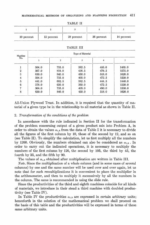
MATHEMATICAL METHODS OF ORGANIZING AND PLANNING PRODUCTION 411
TABLE II
1 2 3 4 5
10 percent 12 percent 28 percent 36 percent 14 percent
TABLE III
Type of Material Machine
No.~~~~~~~~~~~~~~~~~~~~~~~~~~~~~~~~~~~~~~~~~~~~~~~~~~~~~~~~~~~~~~~~~~~~~~~~~~~~~~~~~~~~~~~~~~~~~~~~~~~~~~~~~~~~~~~~~~~~~~~~~~~~~~~~~~~~~~~~~~~~~ 1 ~ ~~2 3 4 5
1 504.0 735.0 382.5 455.0 1485.0 2 567.0 819.0 436.5 479.5 1575.0 3 630.0 840.0 450.0 518.0 1620.0 4 504.0 735.0 405.0 472.5 1530.0 5 441.0 682.5 382.5 444.5 1440.0 6 378.0 630.0 360.0 472.5 1350.0 7 504.0 735.0 405.0 490.0 1530.0 8 630.0 840.0 450.0 518.0 1620.0
All-Union Plywood Trust. In addition, it is required that the quantity of ma- terial of a given type be in the relationship to all material as shown in Table II.
2. Transformation of the conditions of the problem
In accordance with the rule indicated in Section II for the transformation of the problem concerning output of a given product mix into Problem A, in order to obtain the values ai,k from the data of Table I it is necessary to divide all the figures of the first column by 10, those of the second by 12, and so on (see Table II). To simplify the calculation, let us first multiply all the numbers by 1260. Obviously, the numbers obtained can also be considered as ai,k. fIn order to carry out the indicated operations, it is necessary to multiply the numbers of the first column by 126, the second by 105, the third by 45, the fourth by 35, and the fifth by 90.
The values of ai,k obtained after multiplication are written in Table III. Note. Since the multiplication of a whole column (and in some cases of several
columns) by one and the same number will be used over and over again, let us note that for such remultiplications it is convenient to place the multiplier in the arithmometer, and then to multiply it successively by all the numbers in the column. The same is recommended in using the slide rule.
Since the productivities of the third and eighth machines coincide for all kinds of materials, we introduce in their stead a third machine with doubled produc- tivity (see Table IV).
In Table IV the productivities ai,k are expressed in certain arbitrary units; henceforth in the solution of the mathematical problem we shall proceed on the basis of this table and the productivities will be expressed in terms of these same arbitrary units.

412 L. V. KANTOROVICH
TABLE IV
Type of Material Machine
1 ~ ~~2 3 4 5
1 504.0 735.0 382.5 455.0 1485.0 2 567.0 819.0 436.5 479.5 1575.0 3 1260.0 1680.0 900.0 1036.0 3240.0 4 504.0 735.0 405.0 472.5 1530.0 5 441.0 682.5 382.5 444.5 1440.0 6 378.0 630.0 360.0 472.5 1350.0 7 504.0 735.0 405.0 490.0 1530.0
2; 4158.0 6016.5 3271.5 3850.0 12150.0
20 000 1 4.810 3.324 6.113 5.195 1.646
3. The process of solution
Utilizing the method of resolving multipliers (Appendix I, Sections 3 and 4) for the solution of the problem, we must find numbers X1, X2, X3, X4, X5. For the first approximation XI let us take magnitudes (Table IV, row 9) inversely proportional to the output totals (Table IV, row 8).
Note. Taking the multipliers X with precision to the third place of decimals, we will hereafter be obliged to consider two numbers as equal if their difference does not exceed one thousandth of their magnitude.
Since we must take hi,s = 0 if Xkaxi,k > X8aci,, , for a certain k, then for the first approximation to X, we will divide those values (for each i) which are greater than the rest by the product X8ai,s, .
If the values of X are taken thus, then generally speaking, there will be in each line only one non-zero value of h; that is, altogether there will be n (in our case 7) values and the equations Zk hi,k = 1 and z1 = Z2 = * = Zm will give n + m - 1 (i.e., 11) conditions for the hi,7k. In view of this, the Xk must be chosen such that in four rows there should be two maximum products each. Then we will have 11 non-zero values of hi,k which will determine the 11 equations mentioned above.
Let us note that the selection of Xk is made more complicated by the fact that there is established the restriction that the hi,k ? 0.
4. Calculation of the Xk
As has been said, let us take for the first approximation, Xk0, the numbers of row 9 in Table IV; that is, the first row of Table A.
Let us compute the products Xk0cai,k (Table V1). In each row we italicize the largest number. In accordance with the remarks
made earlier, in the first line the numbers 2443.1 (of the second column) and 2444.3 (in the fifth column) must be considered to be the same.
Under the k-th column we write the total output of those machines for which

MATHEMATICAL METHODS OF ORGANIZING AND PLANNING PRODUCTION 413
TABLE A
Line 1 2 3 4 5
1 XO 4.810 3.324 6.113 5.195 1.646 2 1 1 1.017 1 1 3 1 1.083 1.083 1 1 4 e3 1 1 1 1 1.082 5 e4 1 1 1 1.111 1
6 e5 1.003 1 1.003 1.003 1
7 X 4.824 3.600 6.753 5.789 1.781
TABLE V1
1 ~~~2 3 4 5
1 2424.2 2443.1 2338.2 2363.7 2444.3 2 2727.3 2722.4 2668.3 2491.0 2592.5 3 6060.6 5584.5 5501.7 5382.0 5338.0 4 2424.2 2443.1 2475.8 2454.6 2518.4 5 2121.2 2268.6 2338.2 2309.2 2370.2 6 1818.2 2094.1 2200.7 2454.6 2222.1 7 2424.2 2448.1 2475.8 25&45.6 2518.4
1827.0 0 0 962.5 2970.0 735.0 1485.0
the products Xkai,k are italicized, as for example in the first column we write the output of the second and third machines on the first material (Table IV) that is 567.0 + 1260.0 = 1827.0; under the third column there will be a zero, since in column three there is not even one italicized number. Thus, there will be shown in row 8 only the output of those machines for which one number has been italicized. In Table V1 in the first row two numbers have been italicized, and so we place the outputs not in row 8, but below, in row 9. If (see the following table) some other row would contain several numbers, then we would place corresponding outputs below, that is in row 10, and so on. The convenience of this notation is explained by the fact that it is necessary for there to be two numbers each in four of the rows that are separated out. At the same time the values of hi,k corresponding to the numbers separated out must be positive and not greater than one, and the outputs for all columns must be equal. In view of this, it is important to know the outputs for each column. Moreover, if the italicized number is in a row in which all the other numbers are smaller, the corresponding output is wholly of the given material (in this case hi,k = 1). If there is a number equal to the given one, the output goes only partially into the productivity of that row; (i.e., hi,k < 1).
The outputs in Table V1 appear as follows: in the first column, 1827.0 conven- tional units; second, from 0 to 735 conventional units; third, 0; fourth, 962.5

414 L. V. KANTOROVICH
conventional units; and fifth from 2970 to 4455 conventional units; that is, the outputs can by no means be equal.
We will increase the lagging columns. For this we introduce correction factors Ek1 for the Xk0. We will first increase the third column.
Turning to Table V1, we note that if we are going to increase the numbers of the third column, it is the number in row 5 which first approaches its maximum. But since the output of the fifth machine on the third material is equal to only 382.5 conventional units, which is even less than its productivity on the second material, it is clearly necessary to increase the numbers of the third column in such a way that the maximum will be reached in another row, namely the fourth row. In order to find El, let us divide the largest number in the fourth row, 2518.4, by 2475.8, and the other Ek1 let us make equal to unity (see the second row of Table A).
After multiplying the values of Table V1 (specifically the third column) by Ekt we obtain Table V2.
Now it is materials 2 and 3 which have the smallest (approximately equal) outputs. Therefore we will increase them at the same time; that is, let us set for the second correction factors E22 = E32 = E.
TABLE V2
1 ~ ~~2 3 4 5
1 2424.2 2443.1 2377.9 2363.7 2444.3 2 2727.3 2722.4 2713.7 2491.0 2592.5 3 6060.6 5584.3 5595.2 5382.0 5333.0 4 2424.2 2443.1 2517.9 2454.6 2518.4 5 2121.2 2268.6 2377.9 2309.2 2370.2 6 1818.2 2094.1 2238.1 2454.6 2222.1 7 2424.2 2443.1 2517.9 2545.6 2518.4
1827.0 0 382.5 962.5 0 735.0 1485.0
405.0 1530.0
TABLE V3
1 ~ ~~2 3 4 5
1 2424.2 2645.9 2575.3 2363.7 2444.3 2 2727.3 2948.4 2938.9 2491.0 2592.5 3 6060.6 6047.8 6059.6 5382.0 5333.0 4 2424.2 2645.9 2726.9 2454.6 2518.4 5 2121.2 2456.9 2575.3 2309.2 2370.2 6 1818.2 2267.9 2423.9 2454.6 2222.1 7 2424.2 2645.9 2726.9 2545.6 2518.4
0 1554.0 992.5 472.5 0 1260.0 900.0

MATHEMATICAL METHODS OF ORGANIZING AND PLANNING PRODUCTION 415
TABLE V4
1 ~~~2 3 43
1 2424.2 2645.9 2575.3 2363.7 2644.8 2 2727.3 2948.4 2938.9 2491.0 2805.1 3 6060.6 6047.8 6059.6 5382.0 5770.3 4 2424.2 2645.9 2726.9 2454.6 2724.9 5 2121.2 2456.9 2575.3 2309.2 2564.6 6 1818.2 2267.9 2423.9 2454.6 2404.3 7 2424.2 2645.9 2726.9 2545.6 2724.9
0 819.0 382.5 472.5 0 1260.0 900.0
735.0 1485.0 810.0 3060.0
In choosing e let us note that the first number to approach the maximum value in its row is the number in the 7th row of the third column, but in this instance this cannot satisfy us; we cannot both do this and at the same time achieve the maximum value with the number in the second row of the second column; we thus arrange for the number in the third row of the third column to approach the maximum.
We find that e = s 95:2 = 1.083. The other Ek2 = 1 (Table A, row 3). Multi- plying by these factors we obtain the values of XkaZ,k for the third approximation (Table V3).
Increasing the number of the fifth column (the fourth row of Table A), we obtain the same values for the fourth approximation (Table V4).
Note that although in Table V4 we have 11 non-zero values of hi,k, still the remaining values for hi,k within the limits from 0 to 1 do not permit us to achieve equality for the outputs of all the columns. (Let us also note that the coincidence of maximum values in rows 4 and 7 between columns 3 and 5 is accidental.)
Increasing the fourth column, we arrange it so that the numbers in this column become maximal not only in the seventh row but also in the fourth row (Table V5).
Everything that was noted after Table V4 also remains true with respect to Table V5 although here it is rather more difficult to show the impossibility of positive solutions for all hi,k . To establish this, it is necessary to solve a system of equations.)
We increase the numbers of the first, third and fourth columns simultaneously. Thanks to this, we retain two italicized values in each of two rows (the third and fourth). In addition, as before, two maximal values remain in the first row. Increasing the numbers of the three columns we succeed in obtaining two maxi- mum numbers in still another row.
The first number to achieve the maximum value is the number in the second row of the third column. To accomplish this it is necessary to multiply by E3' = 2 9 3 8.9
= 1.003 (see line 6 of Table A). 2 94 8.4

416 L. V. KANTOROVICH
TABLE V5
. 2 3 4 5
1 2424.2 2645.9 2575.3 2626.1 2644.8 2 2727.3 2948.4 2938.9 2767.5 2805.1 3 6060.6 6047.8 6059.6 5979.4 5770.3 4 2424.2 2645.9 2726.9 2727.1 2724.9 5 2121.2 2456.9 2575.3 2565.5 2564.6 6 1818.2 2267.9 2423.9 2727.1 2404.3 7 2424.2 2645.9 2726.9 2828.2 2724.9
0 819.0 382.5 962.5 0 1260.0 900.0
735.0 1485.0 405.0 472.5 1530.0
TABLE V6
1 ~ ~~2 3 4 5
1 2431.5 2645.9 2583.0 2634.0 2644.8 2 2735.5 2948.4 2947.7 2775.8 2805.1 3 6078.8 6047.8 6077.8 5997.3 5770.3 4 2431.5 2645.9 2735.1 2735.8 2724.9 5 2127.6 2456.9 2583.0 2573.2 2564.6 6 1823.7 2267.9 2431.2 2735.2 2404.3 7 2431.5 2645.9 2735.1 2836.7 2724.9
0 0 382.5 962.5 0 1260.0 900.0
735.0 1485.0 819.0 436.5
405.0 472.5
According to Table V6, the output of the first column varies from 0 to 1260.0 conventional units; that of the second from 0 to 1554 conventional units; that of the third from 382.5 to 2124.0 conventional units; that of the fourth from 962.5 to 1435.0 conventional units; and that of the fifth from 0 to 1485.0 con- ventional units. The value of output for all columns is of the same order, and the number of hi,k not equal to zero is 11.
5. Computation of the hi,k
Setting hi,k = 0, if the number in the i-th line of the k-th column of Table V6 is not italicized we obtain for the other hi,k the equations
1260h3,j = 819h2,2 + 735h1,2 = 436.5h2,3 + 900h3,3 + 405h4,3 + 382.5h5,3 = 472.5h4,4 + 472.5h6,5 + 490h7,4 = 1485h1,5;
hl,2 + hl,3 = 1; h2,2 + h2,3 = 1; h3,1 + h3,3 = 1; h4,3 + h4,4 = 1; h5,3 = 1;h6,4 = 1;h7,4= 1.
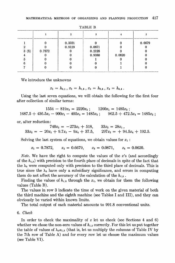
MATHEMATICAL METHODS OF ORGANIZING AND PLANNING PRODUCTION 417
TABLE B
1 2 3 4 5
1 0 0.3321 0 0 0.6679 2 0 0.9129 0.0871 0 0 3 (8) 0.7872 0 0.2128 0 0 4 0 0 0.9380 0.0620 0 5 0 0 1 0 0 6 0 0 0 1 0 7 0 0 0 1 0
We introduce the unknowns
x= h3,1 , x2 = hi,5 , x3 = h25, X4 = h44
Using the last seven equations, we will obtain the following for the first four after collection of similar terms:
1554 - 819x3 = 2220x2; 1260x1 = 1485x2; 1687.5 + 436.5x3 - 900xl - 405x4 = 1485x2; 962.5 + 472.5x4 = 1485x2;
or, after reduction: 740x2 = -273x3 + 518, 33x2 = 28x1,
33x2 = - 20x1 + 9.7x3 - 9x4 + 37.5, 297x2 = + 94.5x4 + 192.5.
Solving the last system of equations, we obtain values for xl:
xi = 0.7872, x2 = 0.6679, X3 = 0.0871, X4 = 0.0620.
Note. We have the right to compute the values of the x's (and accordingly of the hi,k) with precision to the fourth place of decimals in spite of the fact that the Xk were computed only with precision to the third place of decimals. This is true since the Xk have only a subsidiary significance, and errors in computing them do not affect the accuracy of the calculation of the hi,k .
Finding the values of hi,k through the xi, we obtain for them the following values (Table B).
The values in row 3 indicate the time of work on the given material of both the third machine and the eighth machine (see Tables I and III), and they can obviously be varied within known limits.
The total output of each material amounts to 991.8 conventional units.
6. Check
In order to check the maximality of z let us check (see Sections 4 and 6) whether we chose the non-zero values of hi,k correctly. For this let us put together the table of values of Xkai,k (that is, let us multiply the columns of Table IV by the 7th row of Table A) and for every row let us choose the maximum values (see Table VI).

418 L. V. KANTOROVICH
TABLE VI
1 ~ ~~2 3 45
1 2431.3 2646.0 2583.0 2634.0 2644.8 2 2735.0 2948.4 2947.7 2775.8 2805.1 3 6078.2 6048.0 6077.7 5997.4 5770.4 4 2431.4 2646.0 2735.0 2735.3 2724.9 5 2127.4 2457.0 2583.0 2573.2 2564.6 6 1823.5 2268.0 2431.1 2735.2 2404.4 7 2431.3 2646.0 2735.0 2836.6 2724.9
TABLE VII
1 2 3 4 5
1 0 2.32 0 0 11.02 2 0 7.12 0.84 0 0 3 3.94 0 2.13 0 0 4 0 0 8.44 0.84 0 5 0 0 8.50 0 0 6 0 0 0 13.50 0 7 0 0 0 14.00 0 8 3.94 0 2.13 0 0
Total 7.88 9.44 22.04 28.34 11.02
For checking hi,k let us calculate the output for each material: Ist material (1260) (0.7872) = 991.9 conventional units; 2nd material (735) (0.3321) + (819) (0.9129) = 991.8 conventional units; 3rd material (436.5) (0.0871) + (900)(0.2128) + (405) (0.9380) + 382.5 =
991.9 conventional units; 4th material (472.5) (0.0620) + 962.5 = 991.8 conventional units; 5th material (1485) (0.6679) = 991.8 conventional units.
7. Productivity of the machines
Let us calculate the output by materials directly for the data of the Central Laboratory of the All-Union Plywood Trust (Table I). The results are given in Table VII.
8. Comparison with the simplest solution
To calculate the economic effect of the solution determined above, we will compare the total output obtained with that which would be obtained if each material were worked on each machine in the given ratios. Carrying out the calculations for the given data (Table IV) it is necessary that each material should be worked on each machine in equal amounts. Let us determine how much of each material the i-th machine will prepare. Let yi be the quantity of material sought in conventional units.
MATHEMATICAL METHODS OF ORGANIZING AND PLANNING PRODUCTION 419
Then yi = ai, lhi, = ai,2hi,2 = ait,3hi,3 = ait,4hi,4 =ai,Bhi,s,
and since hij, + hi,2 + hi,3 + hi,4 + h,5 = 1,
theii
yi 1 1 1 1 1
aij , ati,2 ati,3 ai,4 ai,5
Calculating yi according to the tables of Barlow (inverse magnitudes) we obtain:
y,= 113.2; Y2 = 125.0; Y3 = 264.9; y4 = 116.5; yb = 107.6; Y6 = 101.3; Y7 = 117.5;
and the total output is 946.0 conventional units. The maximum output in relation to the output just calculated is 104.8 per cent. Note. Such a relatively small percentage difference is explained by the fact
that the productivity of the machines according to data of the Central Labora- tory of the All-Union Plywood Trust is almost proportional.
Appendix 3
Theoretical Supplement
(Proof of Existence of the Resolving Multipliers)
In Appendix I it was established that the determination of the numbers hi,k
by means of the resolving multipliers leads to the solution of the problem and a way of finding these resolving multipliers was shown. For practical purposes, this is perhaps sufficient. But, for completeness, it is important to establish the fact that the resolving multipliers always exist. This will show that the method of resolving multipliers will always be applicable to each problem. In view of the facts that ignorance of the proof of the existence of the multipliers in no way interferes with mastering the method or its practical application, and that we also need some rather more advanced mathematical means for this proof, we have considered it better to treat this in a special supplement.
In the exposition of the proof of the existence of the multipliers we will limit ourselves for brevity to Problem A.'5 We consider it useful to introduce two proofs: analytical and geometrical.
1. Analytical proof
We will consider a system of numbers (Xl , X2, * * Xm) subject to the condi- tions: Xk ?0; X1 + X2 + * * * + Xn = 1. For each given system (X1, X2 X * * Xm), let us consider the products Xlai, ,, X2a ,2 2 ... , Xmctai,r, . For those k for which the product Xkai,k is not the largest in its row, let us set hi,k = 0. Then, let
us try to choose the other hi,k in such a way that min(z,, Z2, X * * * Zm) be as large
15 A more complete mathematical discussion will be given in a special mathematical paper by the author.
420 L. V. KANTOROVICH
as possible. Let us denote the maximum value of this minimum by C(X1, X2, ... , Xm). It is evident that this function is bounded. For example, it is clear that C(X1 , X2 *... * Xm) < Zi,k ai,k . This function has an exact upper limit; let us denote it by C*. There exists a sequence of systems
XS (8) OS)\
for which the values C(X1 X2 , Xmt)
approacn C* lim C(X'1), *, * (s)) C*
From the sequence of systems (X("), ,(') X (3)) (s =1 2, .) it is pos- sible to choose a convergent sub-sequence; without loss of generality, we can consider the original sequence as such; that is,
( t1X)t 2 X Xly ) z) A X 2 *
Further, for each s there exists a definite system of numbers { h 8} which leads to the value C(X(), *, X () ). These systems of numbers, passing if necessary to a sub-sequence, we can consider as converging to a definite system:
lim h h2 =hK s-oo
(i = 1, 2, ,n; k 1, 2, **, i).
Since for each s the necessary conditions for h) have been fulfilled, then also in the limit these conditions must also be fulfilled for hi,k. For the system hi,k=
hi,k we obtain -~~~ ~(s) (8) (8)
min(21, Z2. XZm ) limmin(z1,z 2, *'**zm()
-lim CX(8)) ... 2) ***X S)
) = C*
Therefore, C(X1, )2 X.* *, Xn) > C*. Since on the other hand the reverse in- equality is valid, we have
min(21, 22 * X2X,) = C(Xl, 2, ...X C)
Now by changes in Xk we can make all the Zk equal to C*. Actually, if some Zk > C*, then by decreasing the corresponding Xk and by increasing the others proportionately, we can achieve a coincidence in the Xkai,k at the expense of de- creasing this Zk . Since the other Zk cannot all exceed C* at the same time (because that would contradict the definition of C*) then in this way we can gradually approach such values Xi*, X2*, ... X Xm* for which we can choose hi,k so that Zl = Z2 = = Zm = C*. After we have achieved this, the existence of the resolving multipliers can be considered as being established.
2. Geometric proof
Let us consider all possible systems {hi,k} satisfying the conditions hi,k >
0, Ek-, hi,k = 1. To each system of numbers hi,k there corresponds a definite
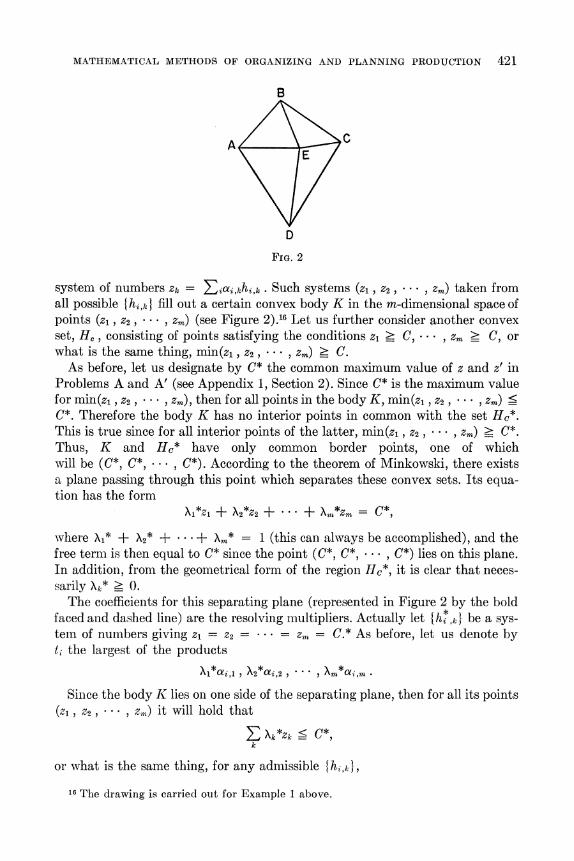
MATHEMATICAL METHODS OF ORGANIZING AND PLANNING PRODUCTION 421
B
A
D
FIG. 2
system of numbers Zk = Z7iiai,khi,k . Such systems (z1, Z2 X * Zm) taken from all possible { hi,k fill out a certain convex body K in the m-dimensional space of points (z1, Z2 , * * , Zm) (see Figure 2).16 Let us further consider another convex set, HC, consisting of points satisfying the conditions zi > C, * Zm > C, or what is the same thing, min(z1, Z2 , * * * , Zm) _ C.
As before, let us designate by C* the common maximum value of z and z' in Problems A and A' (see Appendix 1, Section 2). Since C* is the maximum value for min(zi , Z2 , Zm), then for all points in the body K, min(zi , Z2 Zm) <
C*. Therefore the body K has no interior points in common with the set Hc*. This is true since for all interior points of the latter, min(zi, Z2 , ... * Zm) _ C*.
Thus, K and HC* have only common border points, one of which will be (C*, C*, . , C*). According to the theorem of Minkowski, there exists a plane passing through this point which separates these convex sets. Its equa- tion has the form
X1*zi + X2*Z2 + * + X,,*Zm = C*1
where Xi* + X2* + * * + Xm* = 1 (this can always be accomplished), and the free term is then equal to C* since the point (C*, C*, ... , C*) lies on this plane. In addition, from the geometrical form of the region HC*, it is clear that neces- sarily Xk* ? 0.
The coefficients for this separating plane (represented in Figure 2 by the bold faced and dashed line) are the resolving multipliers. Actually let {I Ii ,k} be a sys- tem of numbers giving z1 = = Z = ZY= C.* As before, let us denote by t1 the largest of the products
Xi* ai,1, X2*ai,2 . * Xm*ai ,m.
Since the body K lies on one side of the separating plane, then for all its points (z1 , * *, z) it will hold that
? Xk*k :_!!< C*>>
or what is the same thing, for any admiissible {h ,k},
16 The drawing is carriecl out for Example 1 above.
422 L. V. KANTOROVICH
Zk* Z a ,k hi,k = Z E\kai,k h,k < C*. k i k
In particular, taking hi,k = 1 for those k for which Xk*ai,k = t , we find that tt < C*. On the other hand,
C= EkZk = k aE,k hk = Z Z (k* ai,k)hk k k
k h k
< 1:ti 1:h*,k = ti i k i
Here, the equality sign in the inequality is achieved only in case hi*,k = 0 when- ever ?,Ak*c,k < ti, but thanks to the inequality found earlier, E ti < C* the equality sign must necessarily be realized here; therefore, the indicated circum- stance for hi,k must take place. Thus, it turns out that for hi,k = h*,k , the condi- tion of being equal to zero is fulfilled for all those which do not correspond to maximal products; and the others are such that zi =Z2 = = Zm . This shows that the X\k* are actually the resolving multipliers, and the existence of the resolv- ing multipliers in Problem A for any case is proved.


![11th International Mathematical - ICME 11Feb6].pdf · 11th International Congress on Mathematical Education ... In parallel, the Local Organizing Committee (LOC), and the Ibero American](https://img.pdfslide.net/doc/110x75/5ad9c5667f8b9ae1768c464b/11th-international-mathematical-icme-11-feb6pdf11th-international-congress-on.jpg)