Mathematical model of crystallization of two-component ...pmw2015.fmi.uni-sofia.bg/Documents/Problem_3_Report.pdf · Mathematical model of the crystallization of two-component alloys

Preparatory Modelling Week, 7 − 11 September, Sofia, Bulgaria

Group 3

Mathematical model of crystallizationof two-component alloys at presence ofnanoparticles

Participant 1: Eliza IlievaFMI, Sofia [email protected]

Participant 2: Lyudmil IovkovFMI, Sofia Universityspider [email protected]

Participant 3: Maria DobrevaFMI, Plovdiv [email protected]

Participant 4: Pavel IlievFMI, Sofia [email protected]

Participant 5: Teodora IvanovaFMI, Sofia Universitytigi [email protected]

Instructor: doc. Valentin ManolovIMS, [email protected]

Instructor: prof. Stefka DimovaFMI, Sofia [email protected]

1

2 Mathematical model of crystallization...

Abstract.Mathematical model of the crystallization of two-component alloys isstudied, analyzed and solved numerically. We have used this model tofind the temperature distribution depending on time for three differentalloys, in particular aluminium alloy, cast iron and carbon steel. It hasbeen found that increasing the number of centers of crystallization byadding nanosized particles reduces the overcooling and thus improvesthe properties of the alloys.Keywords: mathematical modelling, crystallization, overcooling, two-component alloys, nanoparticles

3.1 Introduction

The crystallization is a process of formation and growth of crystals that aremelted from pure substances, alloys, liquids or gas phases. The transition fromliquid to solid state is called primary crystallization. In equilibrium condi-tions the crystallization proceeds with constant temperature or in a temperaturerange. In pure metals only the first case is possible, and both of them in thealloys.

The process begins with pouring the melt into a mould. The temperatureT0 to which the metal is overheated depends on the material, the shape and thesize of the mould. During the crystallization process there are three zones calleda liquid zone, a two-phase zone and an eutectic zone.

The liquid zone starts at the temperature of casting T0 and ends at theliquidus temperature TL. It is known that the crystallization does not beginat the equilibrium liquidus temperature TL but at a lower temperature T . Thevalue ∆T = TL − T is called overcooling.

The two-phase zone starts at the temperature TL and ends at the temperatureTE of the eutectic. The eutectic zone starts at TE .

The process is non-linear due to the complex temperature change in thetwo-phase zone where the centers of crystallization are formed and grow. If theprocess is divided into the three phases mentioned above, only the process in theliquid zone can be treated as linear.

We solve the problem numerically. The purpose of the numerical simulationis to analyze the effect of submission of nanoparticles as additional centers ofcrystallization. It is shown that the inclusion of new centers of crystallizationreduces the overcooling and thus improves the physical properties of the alloys.

3.2 Mathematical model

We consider a small enough specimen about which the temperature T dependsonly on time t and the spatial coordinates are ignored. Using the condition ofheat balance and assuming the case of nonisothermal volume crystallization [1],

3 Preparatory Modelling Week 2015, Sofia, Bulgaria

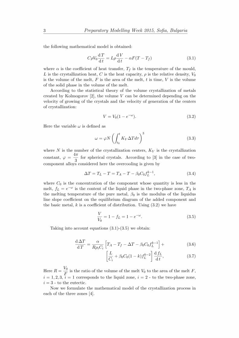
the following mathematical model is obtained:

CρV0dT

d t= Lρ

dV

d t− αF (T − Tf ) (3.1)

where α is the coefficient of heat transfer, Tf is the temperature of the mould,L is the crystallization heat, C is the heat capacity, ρ is the relative density, V0is the volume of the melt, F is the area of the melt, t is time, V is the volumeof the solid phase in the volume of the melt.

According to the statistical theory of the volume crystallization of metalscreated by Kolmogorov [2], the volume V can be determined depending on thevelocity of growing of the crystals and the velocity of generation of the centersof crystallization:

V = V0(1− e−ω). (3.2)

Here the variable ω is defined as

ω = ϕN

(∫ t

t0

KV ∆Tdτ

)3

(3.3)

where N is the number of the crystallization centers, KV is the crystallization

constant, ϕ =4π

3for spherical crystals. According to [3] in the case of two-

component alloys considered here the overcooling is given by

∆T = TL − T = TA − T − β0C0fk−1L , (3.4)

where C0 is the concentration of the component whose quantity is less in themelt, fL = e−ω is the content of the liquid phase in the two-phase zone, TA isthe melting temperature of the pure metal, β0 is the modulus of the liquidusline slope coefficient on the equilibrium diagram of the added component andthe basic metal, k is a coefficient of distribution. Using (3.2) we have

V

V0= 1− fL = 1− e−ω. (3.5)

Taking into account equations (3.1)-(3.5) we obtain:

d ∆T

dT=

α

RρiCi

[TA − Tf −∆T − β0C0f

k−1L

]+ (3.6)[

L

Ci+ β0C0(1− k)fk−2

L

]d fLd t

, (3.7)

Here R =V0F

is the ratio of the volume of the melt V0 to the area of the melt F ,

i = 1, 2, 3, i = 1 corresponds to the liquid zone, i = 2 - to the two-phase zone,i = 3 - to the eutectic.

Now we formulate the mathematical model of the crystallization process ineach of the three zones [4].


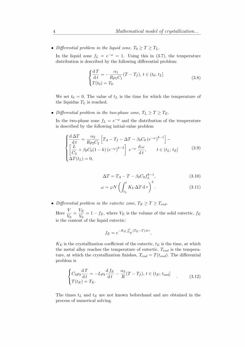
• Differential problem in the liquid zone, T0 ≥ T ≥ TL.

In the liquid zone fL = e−ω = 1. Using this in (3.7), the temperaturedistribution is described by the following differential problem:

dT

d t= − α1

Rρ1C1(T − Tf ), t ∈ (t0; tL]

T (t0) = T0.(3.8)

We set t0 = 0. The value of tL is the time for which the temperature ofthe liquidus TL is reached.

• Differential problem in the two-phase zone, TL ≥ T ≥ TE .

In the two-phase zone fL = e−ω and the distribution of the temperatureis described by the following initial-value problem

d ∆T

d t=

α2

Rρ2C2

[TA − Tf −∆T − β0C0 (e−ω)

k−1]−[

L

C2+ β0C0(1− k) (e−ω)

k−2]e−ω

dω

d t, t ∈ (tL; tE ]

∆T (tL) = 0,

(3.9)

∆T = TA − T − β0C0fk−1L , (3.10)

ω = ϕN

(∫ t

tL

KV ∆T d τ

)3

. (3.11)

• Differential problem in the eutectic zone, TE ≥ T ≥ Tend.

HereV

V0=VEV0

= 1− fE , where VE is the volume of the solid eutectic, fE

is the content of the liquid eutectic:

fE = e−KE

∫ ttE

(TE−T ) d τ,

KE is the crystallization coefficient of the eutectic, tE is the time, at whichthe metal alloy reaches the temperature of eutectic, Tend is the tempera-ture, at which the crystallization finishes, Tend = T (tend). The differentialproblem isC3ρ3

dT

d t= −Lρ3

d fEd t− α3

R(T − Tf ), t ∈ (tE ; tend]

T (tE) = TE .. (3.12)

The times tL and tE are not known beforehand and are obtained in theprocess of numerical solving.


3.3 Numerical methods

We describe the numerical methods used in the three zones and illustrate theresults on the example of an aluminium alloy.

• Liquid zone

The analytical solution of the equation in the liquid zone is

T (t) = Tf + (T0 − Tf )e

α1

Rρ1C1(t0−t)

. (3.13)

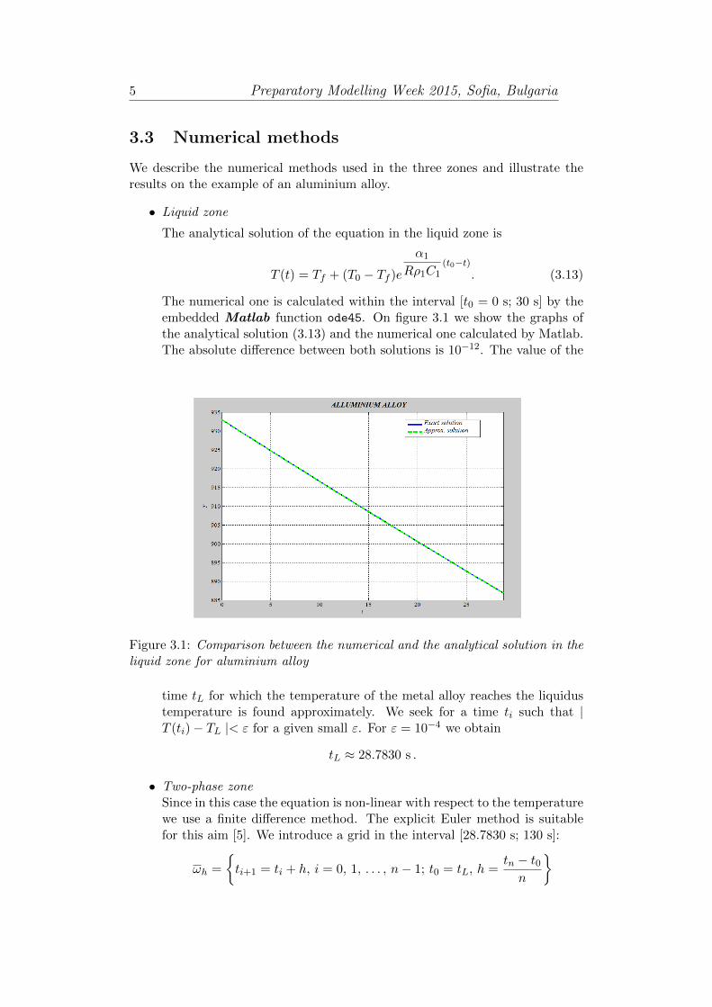
The numerical one is calculated within the interval [t0 = 0 s; 30 s] by theembedded Matlab function ode45. On figure 3.1 we show the graphs ofthe analytical solution (3.13) and the numerical one calculated by Matlab.The absolute difference between both solutions is 10−12. The value of the

Figure 3.1: Comparison between the numerical and the analytical solution in theliquid zone for aluminium alloy

time tL for which the temperature of the metal alloy reaches the liquidustemperature is found approximately. We seek for a time ti such that |T (ti)− TL |< ε for a given small ε. For ε = 10−4 we obtain

tL ≈ 28.7830 s .

• Two-phase zoneSince in this case the equation is non-linear with respect to the temperaturewe use a finite difference method. The explicit Euler method is suitablefor this aim [5]. We introduce a grid in the interval [28.7830 s; 130 s]:

ωh =

{ti+1 = ti + h, i = 0, 1, . . . , n− 1; t0 = tL, h =

tn − t0n

}


and define the mesh function y, the discrete analogue of ∆T . The finitedifference scheme is:

yi+1 = yi +hα2

Rρ2C2

[TA − Tf − yi − β0C0

(e−ωi

)k−1]−

h

[L

C2+ β0C0(1− k)

(e−ωi

)k−2]· e−ωi · ωi − ωi−1

h,

i = 1, 2, . . . , n− 1; y0 = 4T (tL) = 0. (3.14)

For evaluating y2 we need the values of y0 and y1. Since

dω

d t= ϕN · 3

(∫ t

tL

KV ∆T d τ

)2

·KV ∆T (t),

then we havedω

d t(tL) = 0.

From here we calculate

y1 = y0 +hα2

Rρ2C2

[TA − Tf − y0 − β0C0

(e−ω0

)k−1].

We already know the values of y0 and y1. Returning to the explicit Eulermethod (3.14) we successfully obtain the rest of the values of y in the meshnodes.

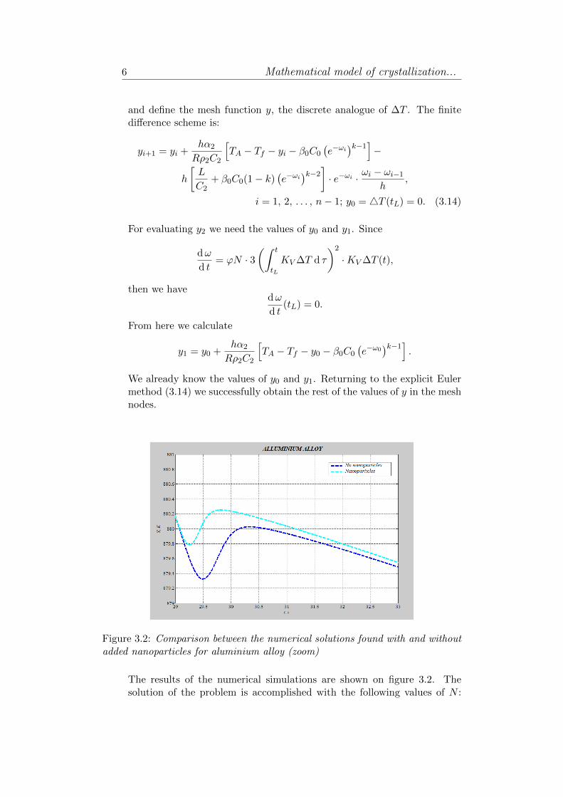
Figure 3.2: Comparison between the numerical solutions found with and withoutadded nanoparticles for aluminium alloy (zoom)

The results of the numerical simulations are shown on figure 3.2. Thesolution of the problem is accomplished with the following values of N :


N = 2.562 · 103 m−3 corresponds to the case without added nanoparticlesand N = 2.562 · 109 m−3 corresponds to the case with added nanoparti-cles. Increasing N we model the increasing of the centers of crystallizationas a result of the added nanosized particles. The graph of the numeri-cal solution of problem 3.2 shows that the increasing of N reduces theovercooling. The magnitude of the supercooling is related to the refiningof the microstructure of the alloy and, hence, it improves its mechanicalproperties.

We find a time tE such that |T (tE) − TE | < ε for arbitrarily small ε. Forε = 10−2 we obtain

tE ≈ 106.03 s .

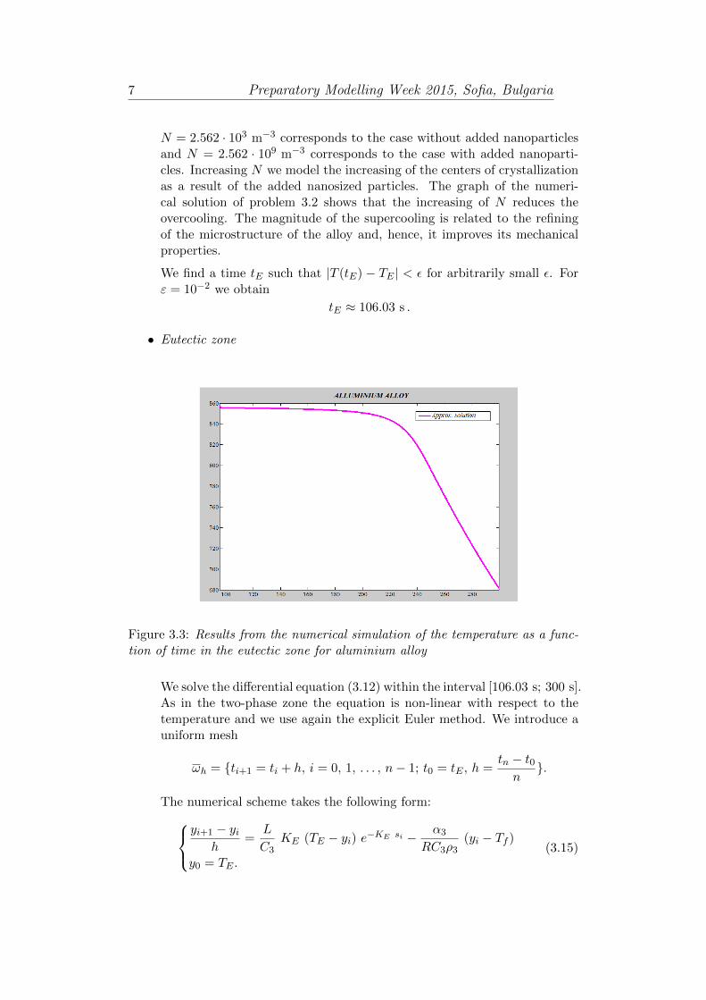
• Eutectic zone

Figure 3.3: Results from the numerical simulation of the temperature as a func-tion of time in the eutectic zone for aluminium alloy

We solve the differential equation (3.12) within the interval [106.03 s; 300 s].As in the two-phase zone the equation is non-linear with respect to thetemperature and we use again the explicit Euler method. We introduce auniform mesh

ωh = {ti+1 = ti + h, i = 0, 1, . . . , n− 1; t0 = tE , h =tn − t0n}.

The numerical scheme takes the following form:yi+1 − yi

h=

L

C3KE (TE − yi) e−KE si − α3

RC3ρ3(yi − Tf )

y0 = TE .(3.15)


Here si is a notation for the integral∫ ti

tE

(TE − T ) d τ.

At first we initialize s0 = 0. Then for each step i we add the value theintegral

∫ titi−1

(TE − T ) d τ to the current value of si−1:

si =

∫ ti

tE

(TE − T ) d τ =

∫ t1

tE

(TE − T ) d τ+∫ t2

t1

(TE − T ) t τ + · · ·+∫ ti−1

ti−2

(TE − T ) d τ +

∫ ti

ti−1

(TE − T ) d τ

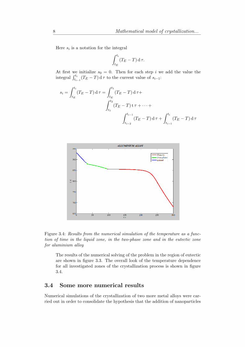
Figure 3.4: Results from the numerical simulation of the temperature as a func-tion of time in the liquid zone, in the two-phase zone and in the eutectic zonefor aluminium alloy

The results of the numerical solving of the problem in the region of eutecticare shown in figure 3.3. The overall look of the temperature dependencefor all investigated zones of the crystallization process is shown in figure3.4.

3.4 Some more numerical results

Numerical simulations of the crystallization of two more metal alloys were car-ried out in order to consolidate the hypothesis that the addition of nanoparticles


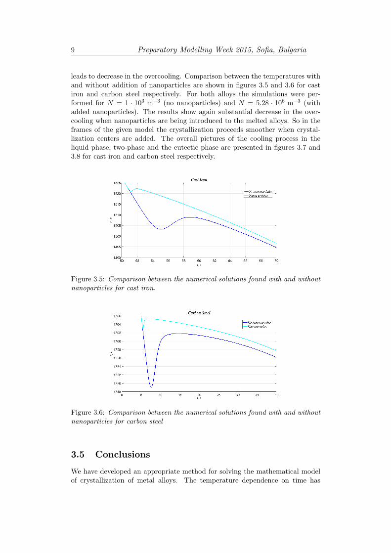
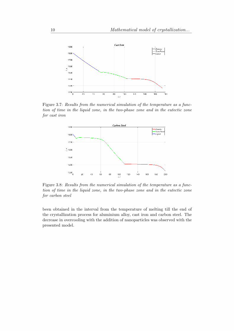
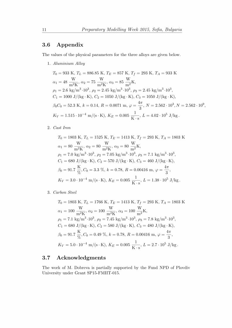
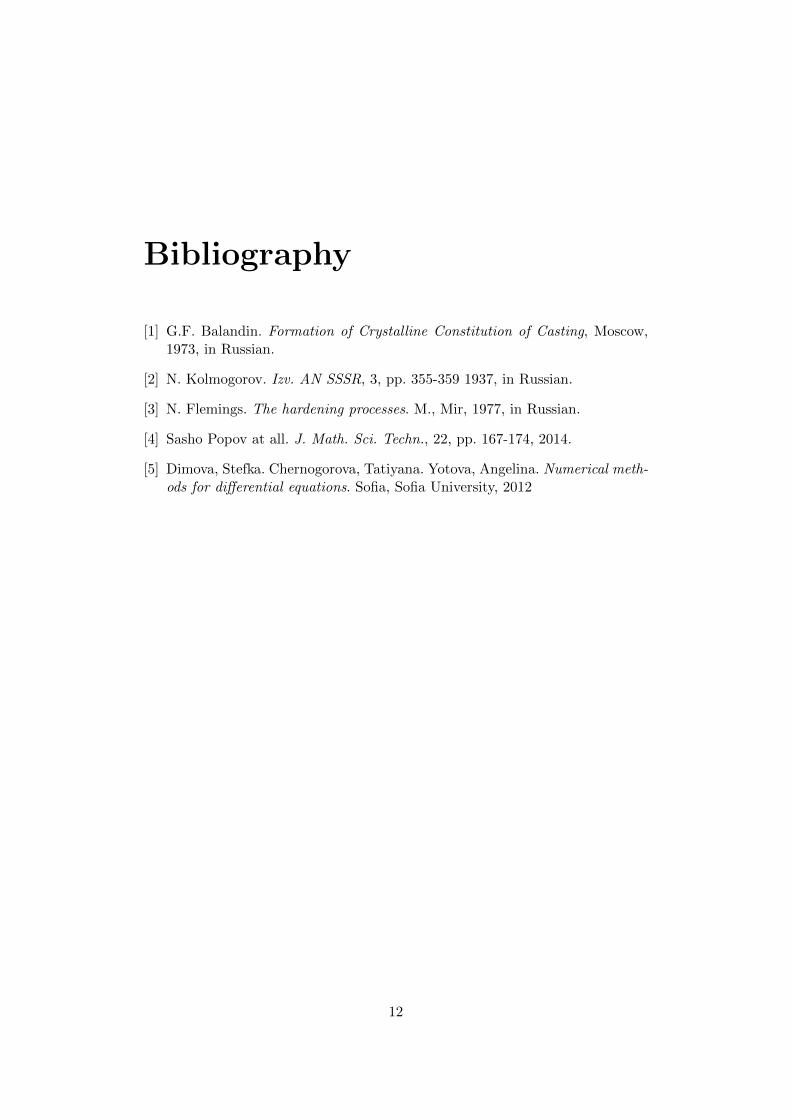
leads to decrease in the overcooling. Comparison between the temperatures withand without addition of nanoparticles are shown in figures 3.5 and 3.6 for castiron and carbon steel respectively. For both alloys the simulations were per-formed for N = 1 · 103 m−3 (no nanoparticles) and N = 5.28 · 106 m−3 (withadded nanoparticles). The results show again substantial decrease in the over-cooling when nanoparticles are being introduced to the melted alloys. So in theframes of the given model the crystallization proceeds smoother when crystal-lization centers are added. The overall pictures of the cooling process in theliquid phase, two-phase and the eutectic phase are presented in figures 3.7 and3.8 for cast iron and carbon steel respectively.

Figure 3.5: Comparison between the numerical solutions found with and withoutnanoparticles for cast iron.

Figure 3.6: Comparison between the numerical solutions found with and withoutnanoparticles for carbon steel

3.5 Conclusions

We have developed an appropriate method for solving the mathematical modelof crystallization of metal alloys. The temperature dependence on time has


Figure 3.7: Results from the numerical simulation of the temperature as a func-tion of time in the liquid zone, in the two-phase zone and in the eutectic zonefor cast iron

Figure 3.8: Results from the numerical simulation of the temperature as a func-tion of time in the liquid zone, in the two-phase zone and in the eutectic zonefor carbon steel

been obtained in the interval from the temperature of melting till the end ofthe crystallization process for aluminium alloy, cast iron and carbon steel. Thedecrease in overcooling with the addition of nanoparticles was observed with thepresented model.


3.6 Appendix

The values of the physical parameters for the three alloys are given below.

1. Aluminium Alloy

T0 = 933 K, TL = 886.85 K, TE = 857 K, Tf = 293 K, TA = 933 K

α1 = 48W

m2K, α2 = 75

W

m2K, α3 = 85

W

m2K,

ρ1 = 2.6 kg/m3 ·103, ρ2 = 2.45 kg/m3 ·103, ρ3 = 2.45 kg/m3 ·103,

C1 = 1000 J/(kg ·K), C2 = 1050 J/(kg ·K), C3 = 1050 J/(kg ·K),

β0C0 = 52.3 K, k = 0.14, R = 0.0071 m, ϕ =4π

3, N = 2.562 · 103, N = 2.562 · 109,

KV = 1.515 · 10−4 m/(s ·K), KE = 0.0051

K · s, L = 4.02 · 105 J/kg .

2. Cast Iron

T0 = 1803 K, TL = 1525 K, TE = 1413 K, Tf = 293 K, TA = 1803 K

α1 = 80W

m2K, α2 = 80

W

m2K, α3 = 80

W

m2K,

ρ1 = 7.0 kg/m3 ·103, ρ2 = 7.05 kg/m3 ·103, ρ3 = 7.1 kg/m3 ·103,


β0 = 91.7K

%, C0 = 3.3 %, k = 0.78, R = 0.00416 m, ϕ =

4π

3,

KV = 3.0 · 10−4 m/(s ·K), KE = 0.0051

K · s, L = 1.38 · 105 J/kg .

3. Carbon Steel

T0 = 1803 K, TL = 1766 K, TE = 1413 K, Tf = 293 K, TA = 1803 K

α1 = 100W

m2K, α2 = 100

W

m2K, α3 = 100

W

m2K,

ρ1 = 7.1 kg/m3 ·103, ρ2 = 7.45 kg/m3 ·103, ρ3 = 7.8 kg/m3 ·103,


β0 = 91.7K

%, C0 = 0.49 %, k = 0.78, R = 0.00416 m, ϕ =

4π

3,

KV = 5.0 · 10−4 m/(s ·K), KE = 0.0051

K · s, L = 2.7 · 105 J/kg .

3.7 Acknowledgments

The work of M. Dobreva is partially supported by the Fund NPD of PlovdivUniversity under Grant SP15-FMIIT-015.

Bibliography

[1] G.F. Balandin. Formation of Crystalline Constitution of Casting, Moscow,1973, in Russian.

[2] N. Kolmogorov. Izv. AN SSSR, 3, pp. 355-359 1937, in Russian.

[3] N. Flemings. The hardening processes. M., Mir, 1977, in Russian.

[4] Sasho Popov at all. J. Math. Sci. Techn., 22, pp. 167-174, 2014.

[5] Dimova, Stefka. Chernogorova, Tatiyana. Yotova, Angelina. Numerical meth-ods for differential equations. Sofia, Sofia University, 2012

12