Mathematical Modeling in Population Dynamics

Glenn Ledder

University of Nebraska-Lincoln

http://www.math.unl.edu/~gledder1

gledder@math.unl.edu

Supported by NSF grant DUE 0536508

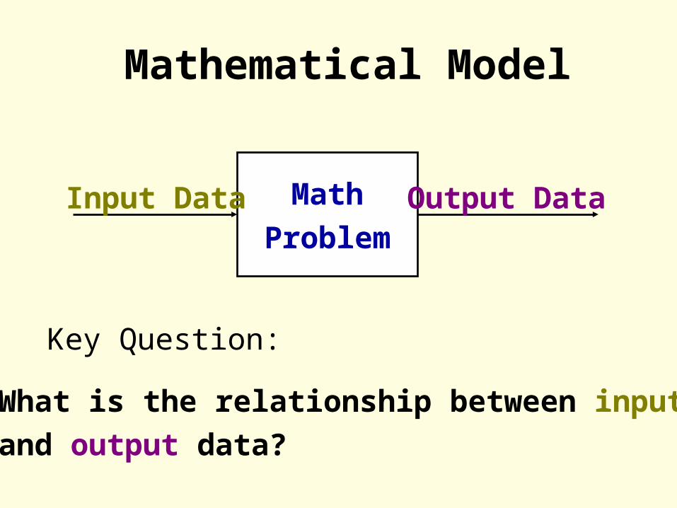
Mathematical Model

Math

ProblemInput Data Output Data

Key Question:

What is the relationship between input

and output data?

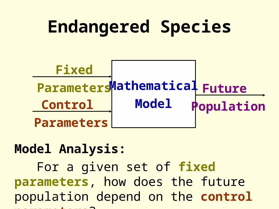
Endangered Species

Mathematical

ModelControl

Parameters

Future

Population

Fixed

Parameters

Model Analysis:

For a given set of fixed parameters, how does the future population depend on the control parameters?

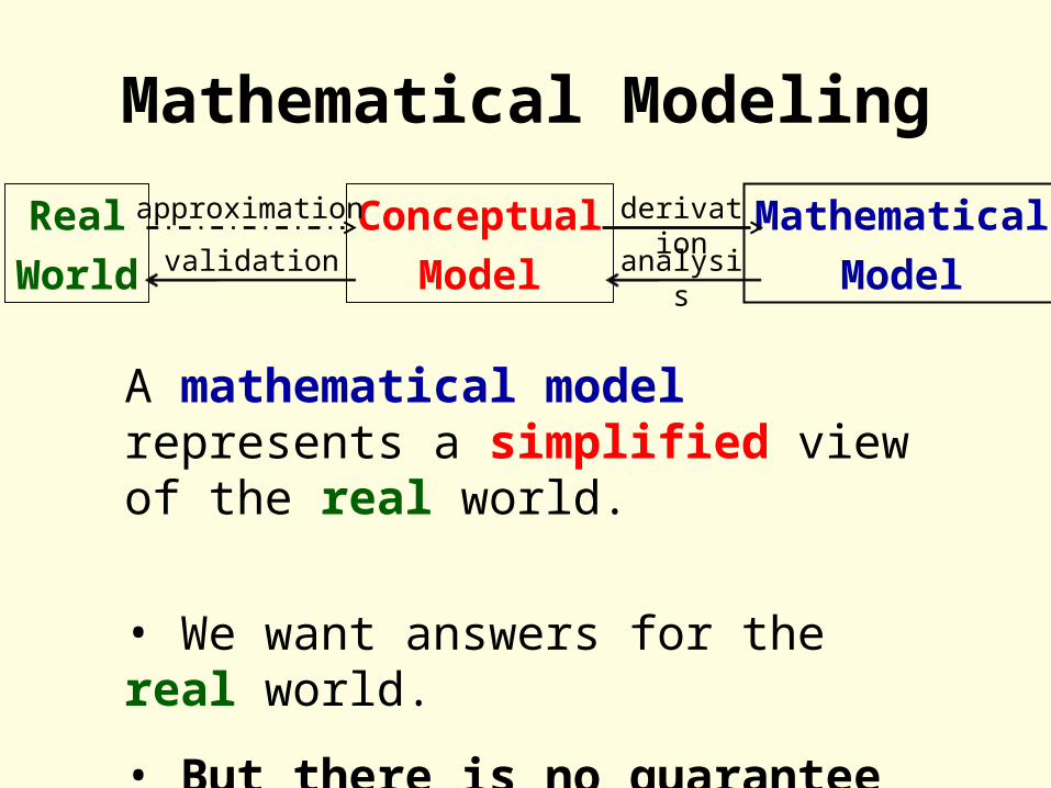
Mathematical Modeling

Real

World

Conceptual

Model

Mathematical

Model

approximation derivation

analysisvalidation

A mathematical model represents a simplified view of the real world.

• We want answers for the real world.

• But there is no guarantee that a model will give the right answers!

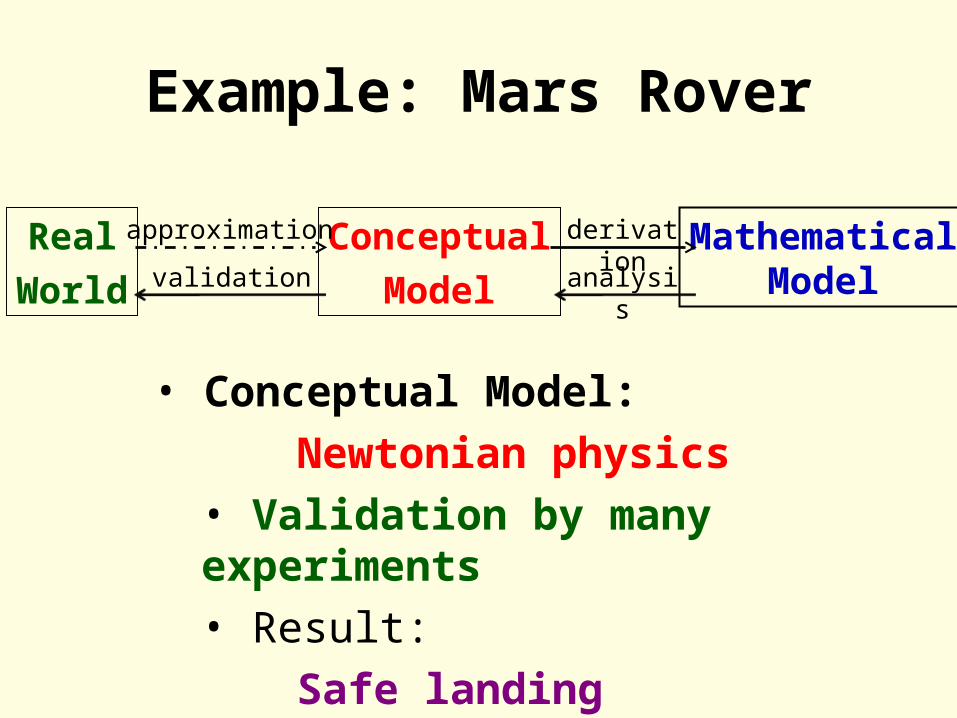
Example: Mars Rover

Real

World

Conceptual

Model

MathematicalModel

approximation derivation

analysisvalidation

• Conceptual Model:

Newtonian physics

• Validation by many experiments

• Result:

Safe landing

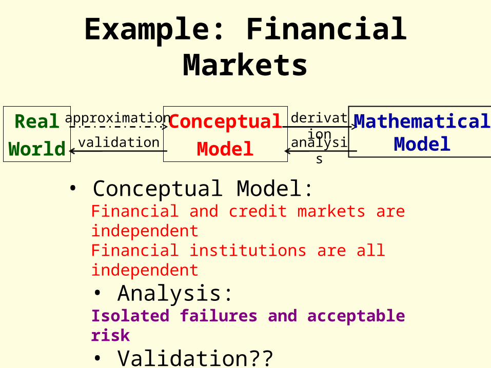
Example: Financial Markets

Real

World

Conceptual

Model

approximation derivation

analysisvalidation

• Conceptual Model:Financial and credit markets are independentFinancial institutions are all independent

• Analysis:Isolated failures and acceptable risk

• Validation??

• Result: Oops!!

MathematicalModel

Forecasting the Election

Polls use conceptual models• What fraction of people in each age group vote?• Are cell phone users “different” from landline users?

and so on

http://www.fivethirtyeight.com• Uses data from most polls• Corrects for prior pollster results• Corrects for errors in pollster conceptual models

Validation?

Most states within 2%!

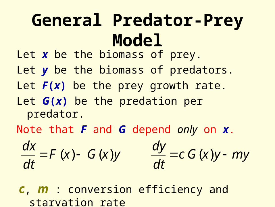
General Predator-Prey ModelLet x be the biomass of prey.

Let y be the biomass of predators.

Let F(x) be the prey growth rate.

Let G(x) be the predation per predator.

Note that F and G depend only on x.

yxGxFdt

dx)()( myyxGc

dt

dy )(

c, m : conversion efficiency and starvation rate

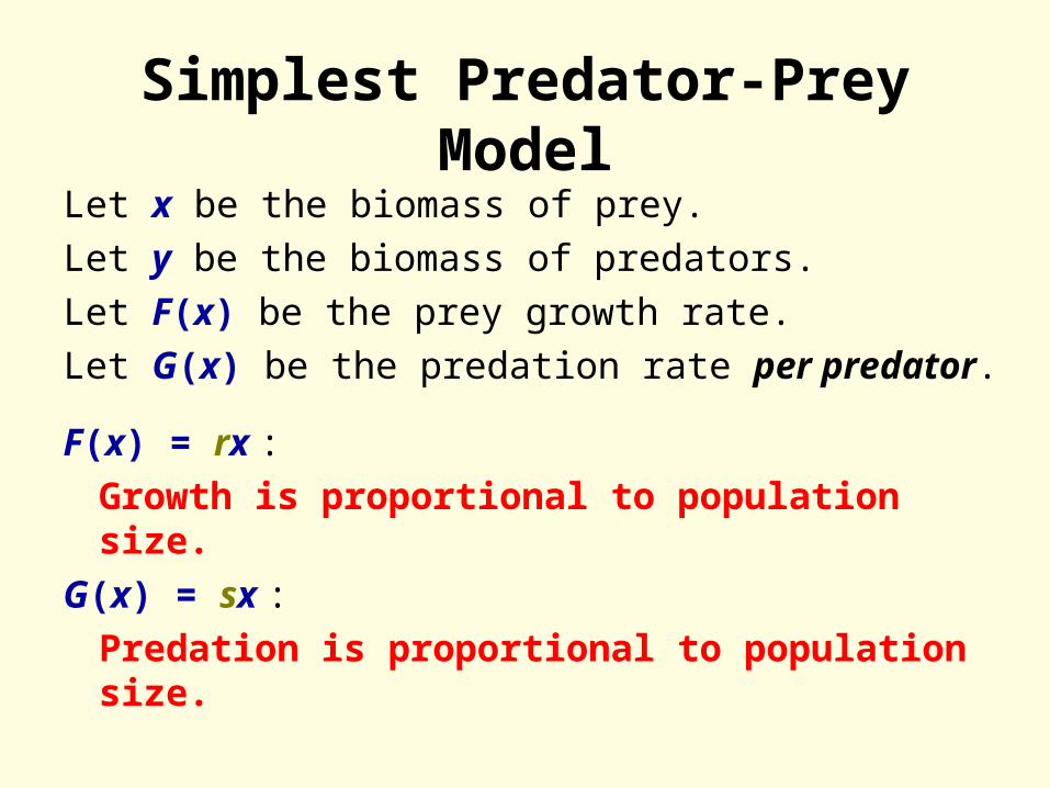
Simplest Predator-Prey Model

Let x be the biomass of prey.

Let y be the biomass of predators.

Let F(x) be the prey growth rate.

Let G(x) be the predation rate per predator.

F(x) = rx :

Growth is proportional to population size.

G(x) = sx :

Predation is proportional to population size.

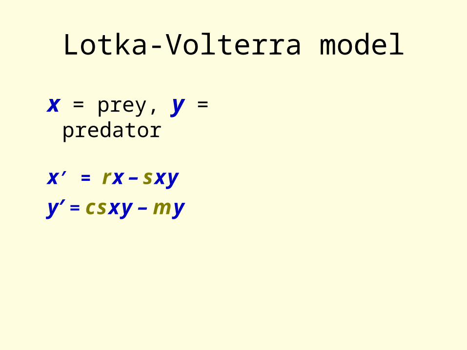
Lotka-Volterra model

x = prey, y = predator

x′ = r x – s x y

y′ = c s x y – m y

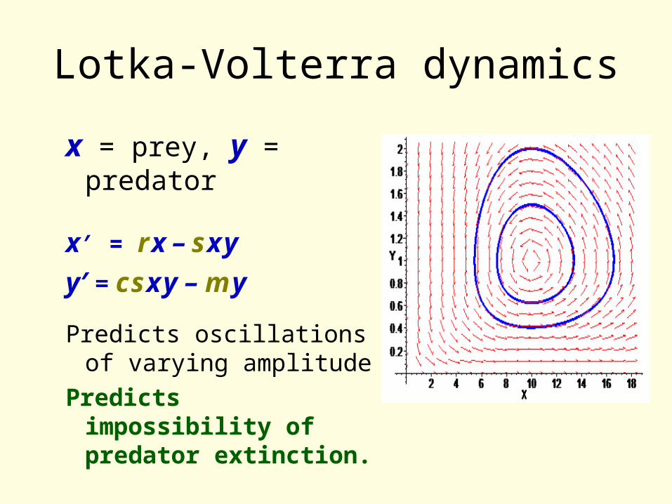
Lotka-Volterra dynamics

x = prey, y = predator

x′ = r x – s x y

y′ = c s x y – m y

Predicts oscillations of varying amplitude

Predicts impossibility of predator extinction.

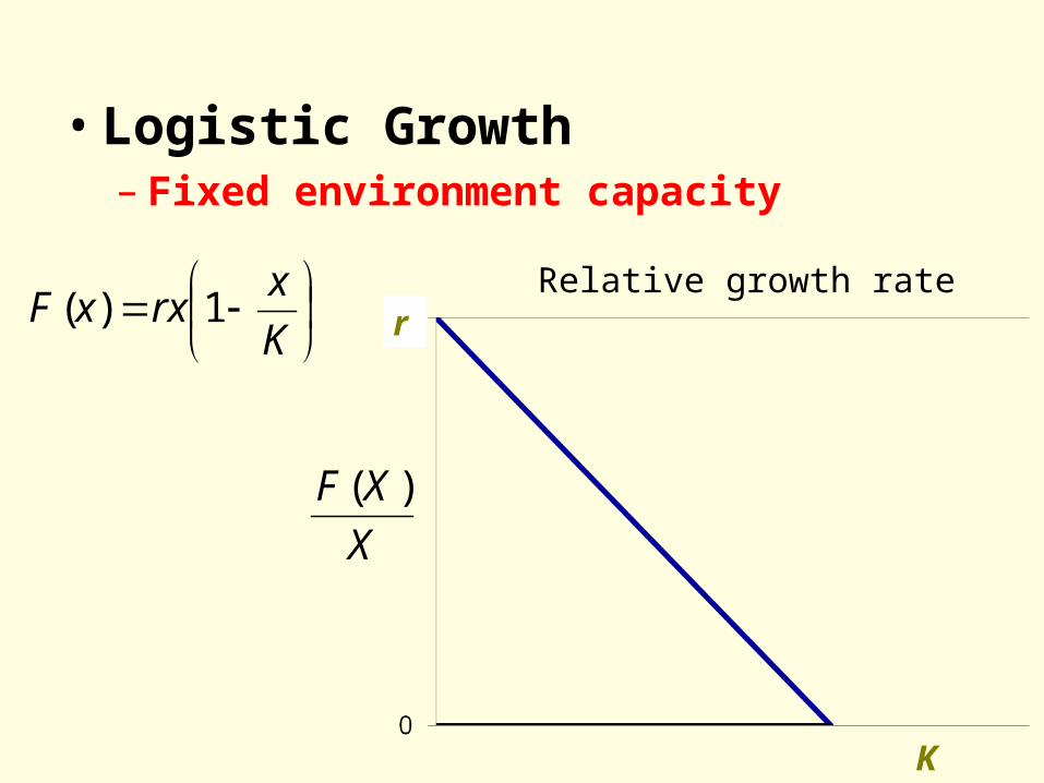
• Logistic Growth– Fixed environment capacity

K

xrxxF 1)(

K

r

X

XF )(

Relative growth rate

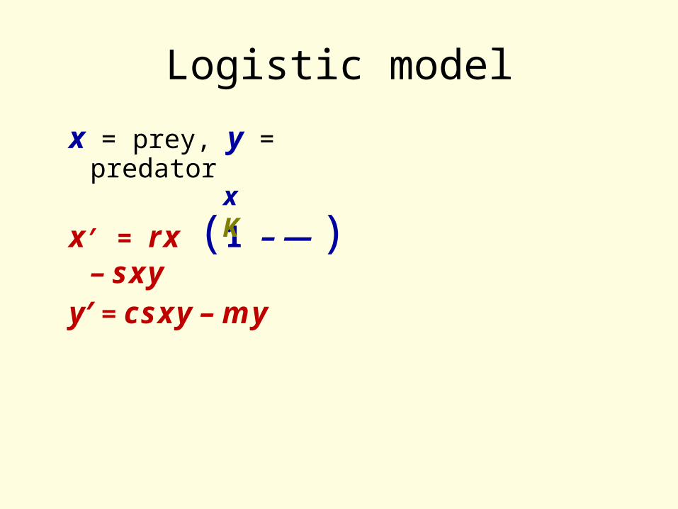
Logistic model

x = prey, y = predator

x′ = r x (1 – — ) – s x y

y′ = c s x y – m y

xK

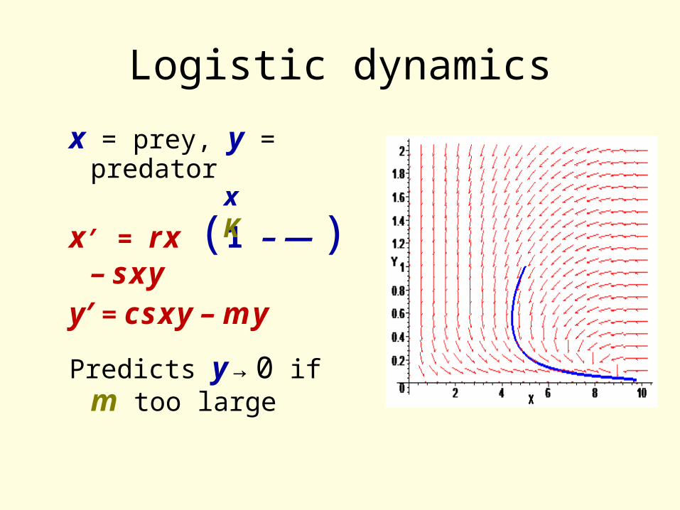
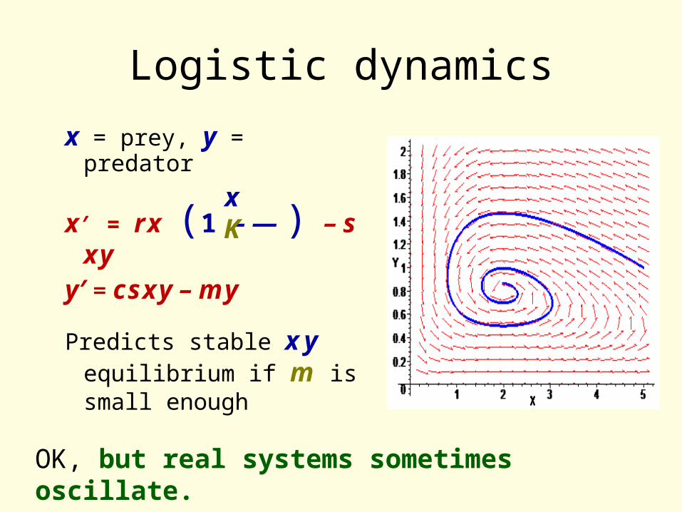
Logistic dynamics

x = prey, y = predator

x′ = r x (1 – — ) – s x y

y′ = c s x y – m y

Predicts y → 0 if m too large

xK

Logistic dynamics

x = prey, y = predator

x′ = r x (1 – — ) – s x y

y′ = c s x y – m y

Predicts stable x y equilibrium if m is small enough

xK

OK, but real systems sometimes oscillate.

Predation with Saturation

• Good modeling requires scientific insight. • Scientific insight requires observation.• Predation experiments are difficult to do in the real world.

• Bugbox-predator allows us to do the experiments in a virtual world.

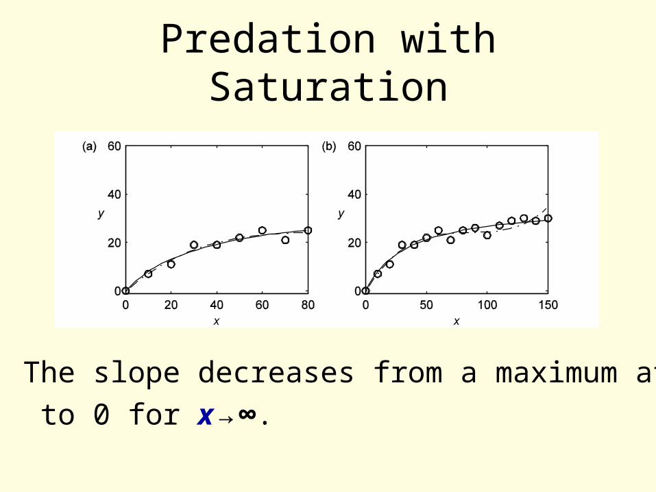
Predation with Saturation

The slope decreases from a maximum at x = 0

to 0 for x → ∞.

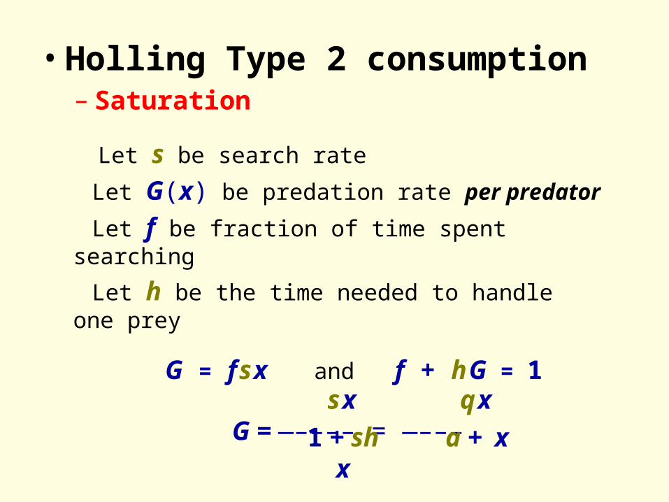
Let s be search rate

Let G(x) be predation rate per predator

Let f be fraction of time spent searching

Let h be the time needed to handle one prey

G = f s x and f + h G = 1

G = —–––– = —–––s x

1 + sh x

q x

a + x

• Holling Type 2 consumption– Saturation

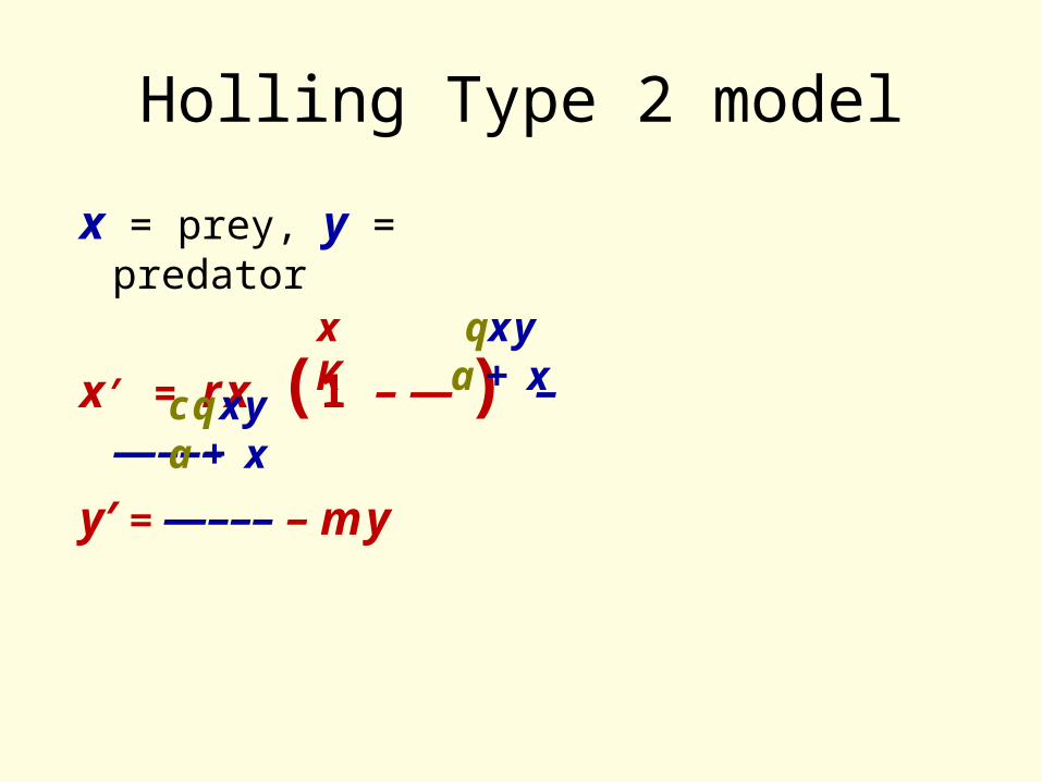
Holling Type 2 model

x = prey, y = predator

x′ = r x (1 – — ) – —–––

y′ = —––– – m y

xK

qx ya + x

c q x ya + x

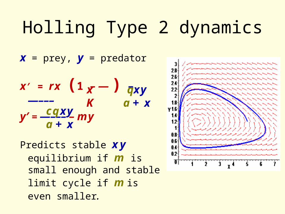
Holling Type 2 dynamics

x = prey, y = predator

x′ = r x (1 – — ) – —–––

y′ = —––– – m y

Predicts stable x y equilibrium if m is small enough and stable limit cycle if m is even smaller.

xK

qx ya + x

c q x ya + x

Simplest Epidemic Model

Let S be the population of susceptibles.

Let I be the population of infectives.

Let μ be the disease mortality.

Let β be the infectivity.

No long-term population changes.

S′ = − βSI:

Infection is proportional to encounter rate.

I′ = βSI − μI :

Salton Sea problem• Prey are fish; predators are birds.• An SI disease infects some of the fish.• Infected fish are much easier to catch than

healthy fish.• Eating infected fish causes botulism

poisoning.

C__ and B__, Ecol Mod, 136(2001), 103:

1.Birds eat only infected fish.

2.Botulism death is proportional to bird population.

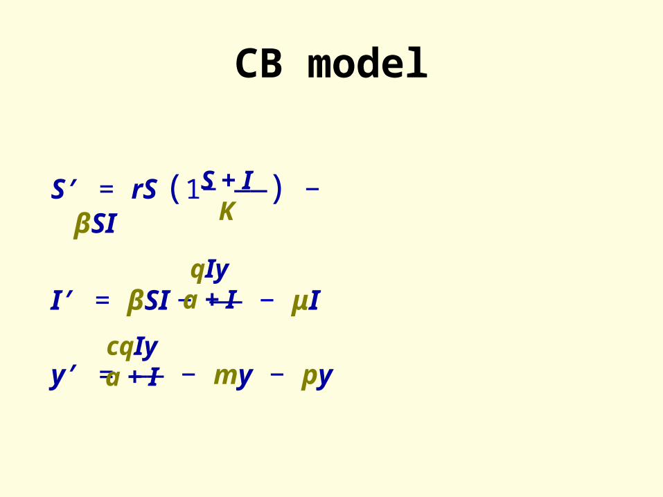
CB model

S′ = rS (1− ——) − βSI

I′ = βSI − —— − μI

y′ = —— − my − py

S + IK

qIya + I

cqIya + I

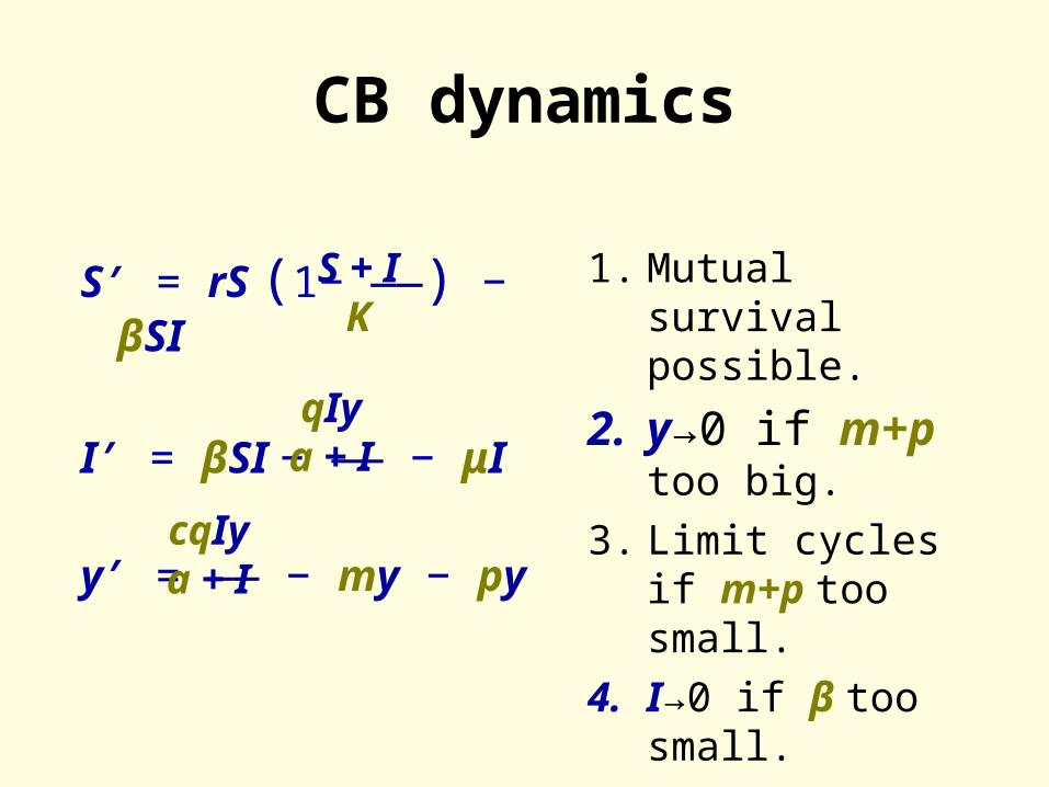
CB dynamics

1. Mutual survival possible.

2. y→0 if m+p too big.

3. Limit cycles if m+p too small.

4. I→0 if β too small.

S′ = rS (1− ——) − βSI

I′ = βSI − —— − μI

y′ = —— − my − py

S + IK

qIya + I

cqIya + I

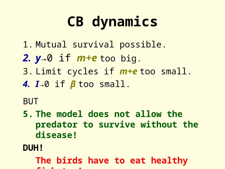
CB dynamics

1. Mutual survival possible.

2. y→0 if m+e too big.

3. Limit cycles if m+e too small.

4. I→0 if β too small.

BUT

5. The model does not allow the predator to survive without the disease!

DUH!

The birds have to eat healthy fish too!

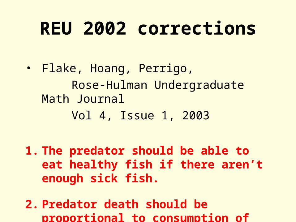
REU 2002 corrections

• Flake, Hoang, Perrigo,

Rose-Hulman Undergraduate Math Journal

Vol 4, Issue 1, 2003

1. The predator should be able to eat healthy fish if there aren’t enough sick fish.

2. Predator death should be proportional to consumption of sick fish.

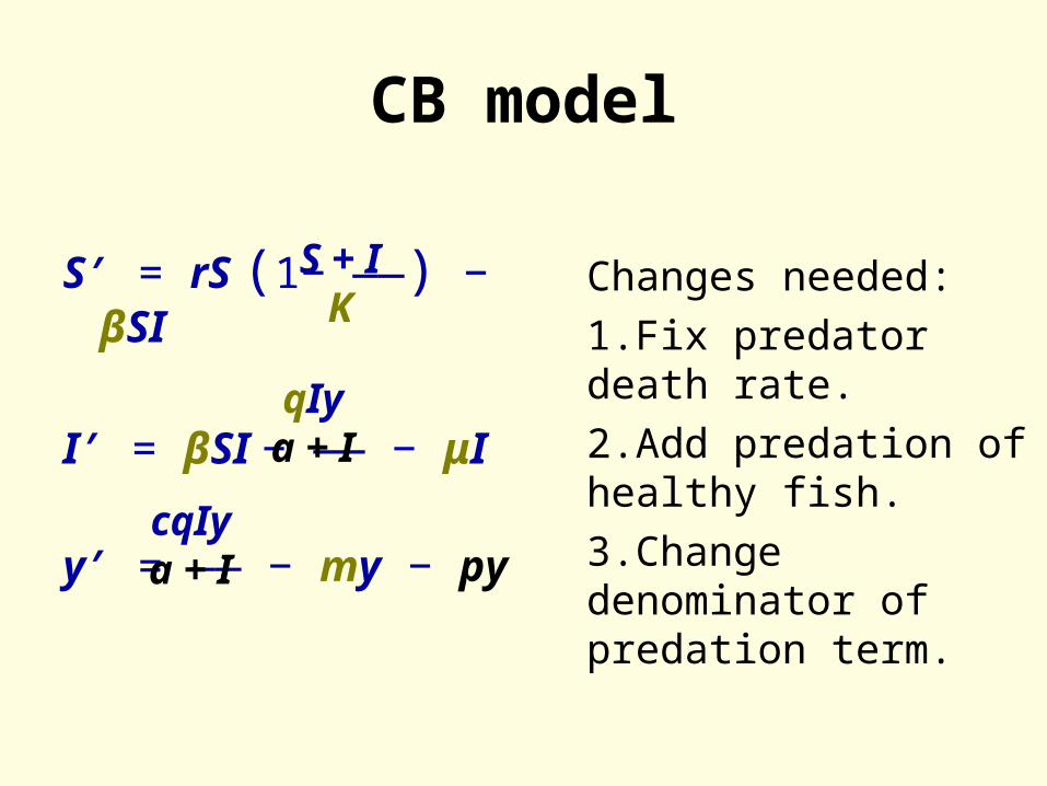
CB model

S′ = rS (1− ——) − βSI

I′ = βSI − —— − μI

y′ = —— − my − py

S + IK

qIya + I

cqIya + I

Changes needed:

1.Fix predator death rate.

2.Add predation of healthy fish.

3.Change denominator of predation term.

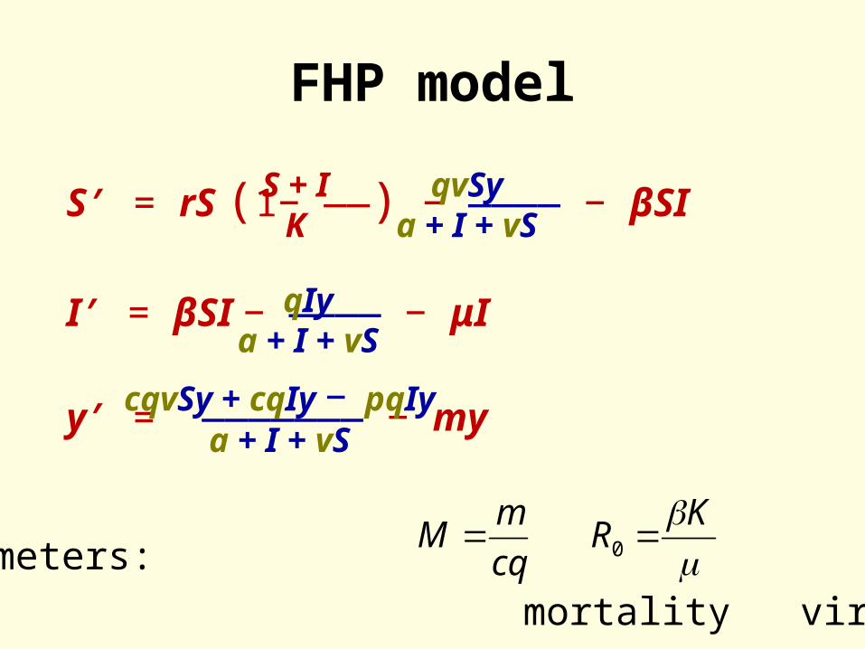
FHP model

S′ = rS (1− ——) − ———— − βSI

I′ = βSI − ———— − μI

y′ = ——————— − my

S + IK

cqvSy + cqIy − pqIya + I + vS

qIya + I + vS

qvSya + I + vS

Key Parameters:

mortality virulencecq

mM

K

R 0

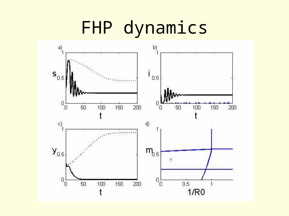
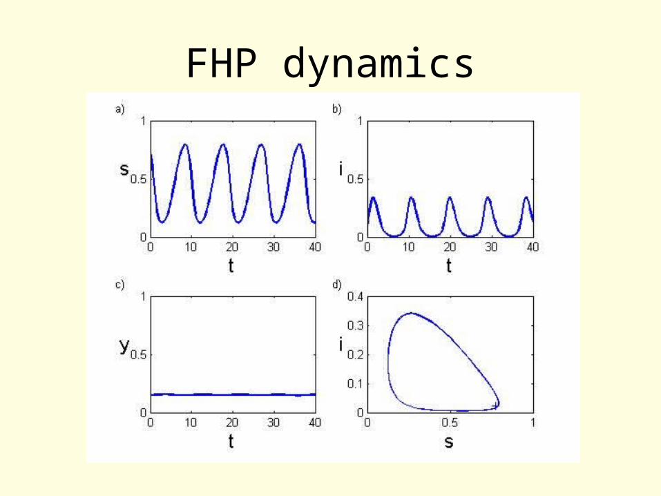
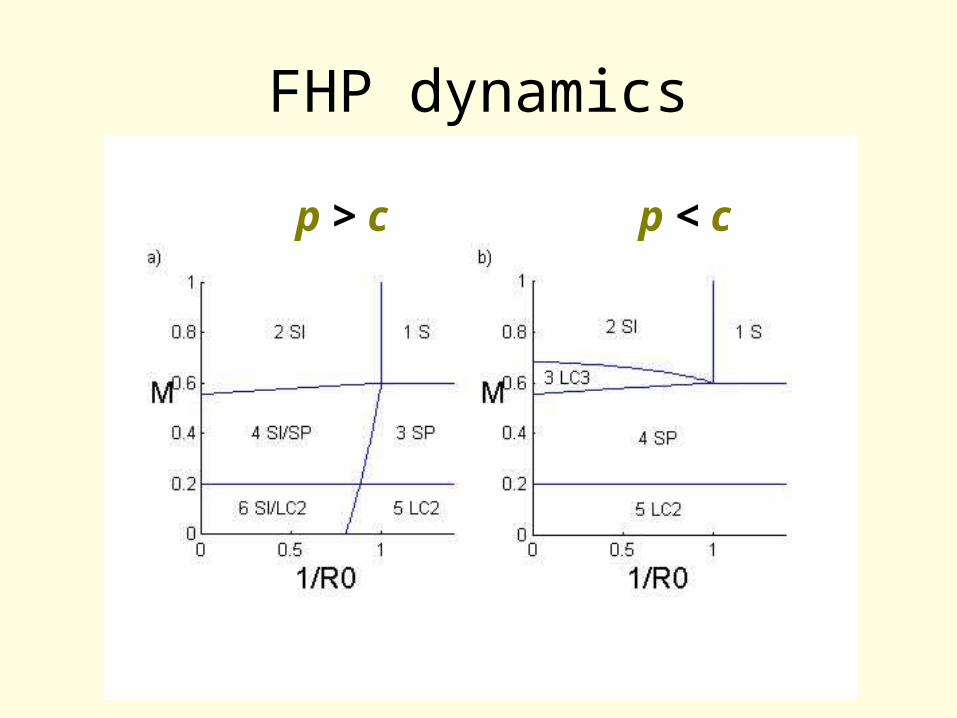
FHP dynamics

p > c p < cp > c p < c

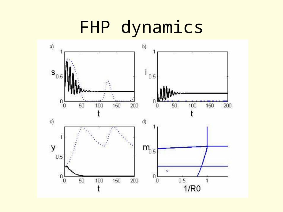
FHP dynamics

FHP dynamics

FHP dynamics

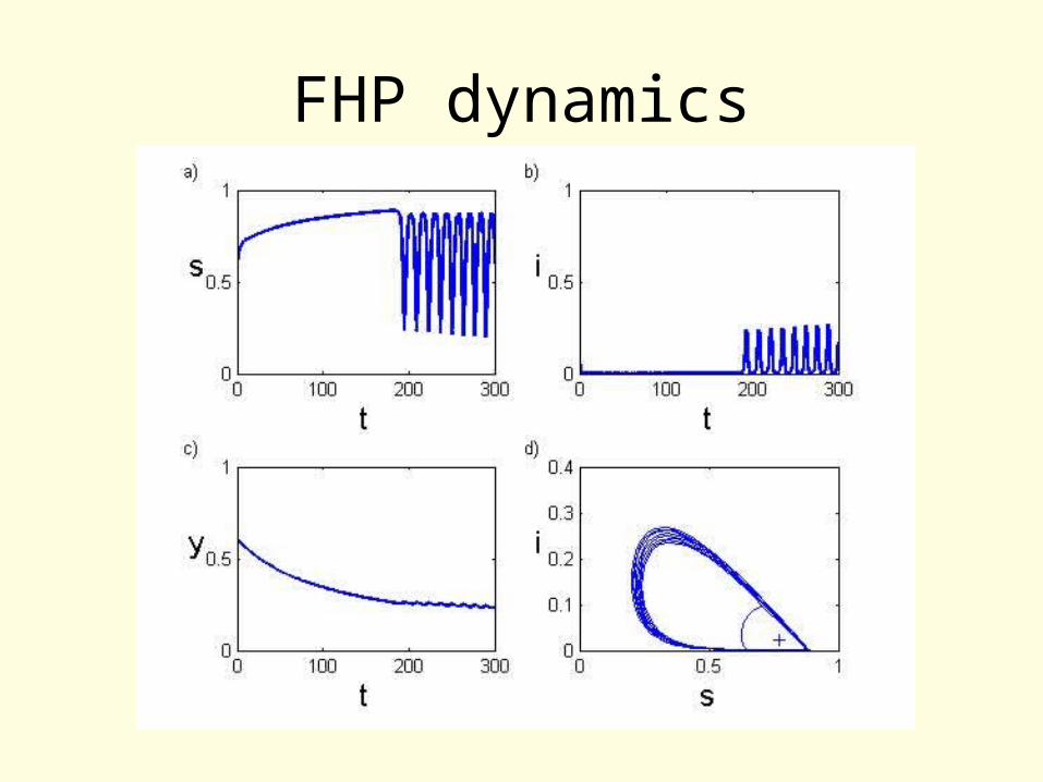
FHP dynamics

FHP dynamics

p > c p < cp > c p < c