Mathematical modeling applications in

water assessment and management

Saurabh Mathur

(National Institute Of Technology-Hamirpur, saurabhmathur2@gmail.com)

1) ABSTRACT

An assessment of the available water resources is a pre-requisite to undertake an analysis of the stress on the water

resources and to subsequently adopt appropriate management strategies to avoid adverse environmental effects and

reconcile conflicts between users.

During the last five decades there has been a sharp increase in water consumption owing to the population

explosion, unprecedented rise in standard of living, and enormous economic development. The situation has become

even more difficult because of the increasing pollution of water resources. This in turn has caused serious problems

impeding sustained economic and social development in many regions, even those not located in arid zones. These

problems are caused not only by natural factors, such as uneven precipitation in space and time, but also by

mismanagement and the lack of knowledge about existing water resources.

Research on the development and application of water balance models at different spatial and temporal scales has

been carried out since later part of the 19th century. As a result, a great deal of experience on various models and

methods has been gained. A large number of models has been proposed in the hydrology field. The various methods

for modeling includes both traditional long-term water balance methods and the new generation distributed models

for assessing available water resources under stationary and changing climatic conditions at different spatial and

temporal scales. Modern models make use of GIS and remote sensing to provide adequate information. Although

these models have progressed fairly through all these years, still they face a lot of challenges.

2) INTRODUCTION

Growing population faces a severe threat of stress due to water scarcity. Problems are

accentuated by excess use of the limited water resources and the deteriorating quality of the

available water. This combined with our lack of knowledge regarding the knowledge of exactly

how much water is available poses difficulties for effective regional, national, and international

water resources management. Moreover, the situation becomes even more complicated by the

looming climate change which, in the longer period has the potential to decrease the availability

of natural water resources in many areas of the world due to probable changes in the rainfall

distribution and the increase in temperature. Due to the complexities, there arises the need to

understand the technical aspects and the broader managerial and social aspects. These aspects are

very well studied using the various mathematical models proposed all along the 19th century.

This paper reviews the existing methods/models for assessing regional water resources under

stationary and changing climate conditions at different spatial and temporal scales, identify the

progress and challenges that remain and discuss the possible further developments in the field. It

discusses the representative methods/models and the different categories of these models instead

of the individual models.

The models can be classified as models under stationary climate change and under constant

climate change. The methods for simulating water resources under stationary climate conditions

includes the long term water balance methods, conceptual lumped-parameter models and spatial

hydrologic GIS supported models.

Methodologies for assessing hydrological responses to global climate change include five

methods which include the use of direct GCM-derived hydrological output, the method of

coupling GCMs and macro scale hydrologic models, the use of dynamic downscaling, the use of

statistical downscaling and the use of hypothetical scenarios as input to hydrological models.

3) WATER RESOURCE MODELING UNDER STATIONARY CLIMATE

These models include the models which are applicable during constant climate. There are a large

number of popular mathematical models of respectively large and small watershed hydrology.

watershed modeling includes data acquisition , model components, model construction,

calibration and verification, analysis of risk and reliability.

3.1) LONG TERM WATER BALANCE METHOD

It is a traditional way for water resources assessment which is based on the long-term average

water balance equation (say one year or many years) over a basin as

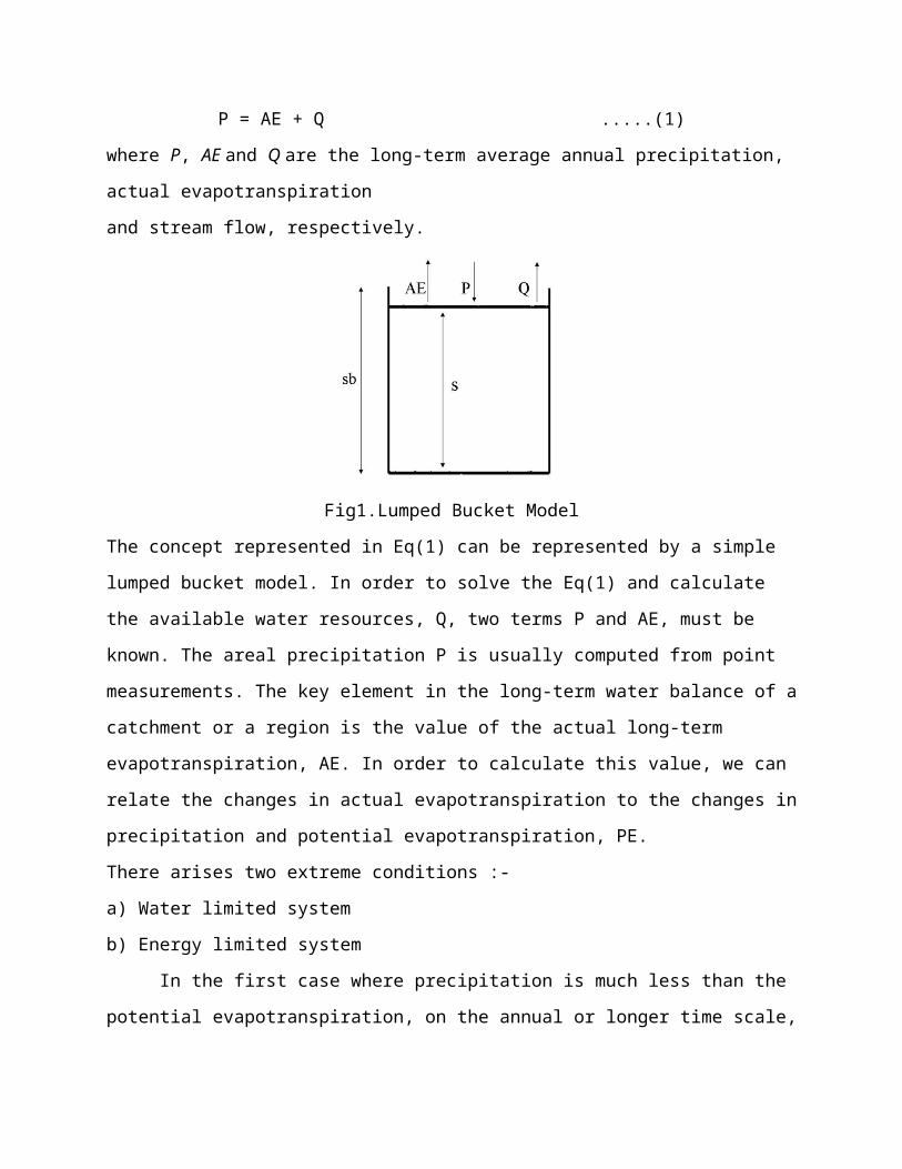
P = AE + Q .....(1)

where P, AE and Q are the long-term average annual precipitation, actual evapotranspiration

and stream flow, respectively.

Fig1.Lumped Bucket Model

The concept represented in Eq(1) can be represented by a simple lumped bucket model. In order

to solve the Eq(1) and calculate the available water resources, Q, two terms P and AE, must be

known. The areal precipitation P is usually computed from point measurements. The key element

in the long-term water balance of a catchment or a region is the value of the actual long-term

evapotranspiration, AE. In order to calculate this value, we can relate the changes in actual

evapotranspiration to the changes in precipitation and potential evapotranspiration, PE.

There arises two extreme conditions :-

a) Water limited system

b) Energy limited system

In the first case where precipitation is much less than the potential evapotranspiration, on the

annual or longer time scale, all incoming precipitation is evaporated back. The actual

evapotranspiration rate is controlled by the amount of rainfall, regardless of how high PE is.

Thus this is a “water limited” system. The first limiting condition occurs when

AE = P and Q = 0 .....(2)

In the second case precipitation is much greater than the potential evapotranspiration, we

would have the second limiting condition

AE = PE and Q = P − AE .....(3)

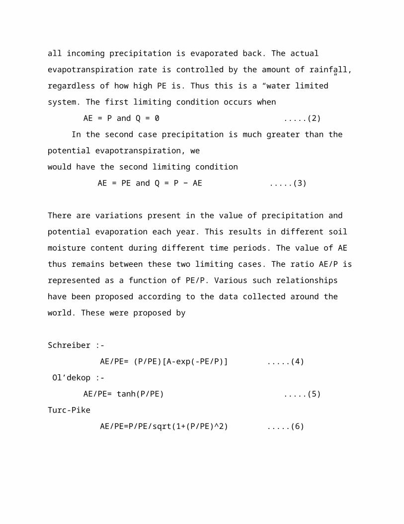
There are variations present in the value of precipitation and potential evaporation each year.

This results in different soil moisture content during different time periods. The value of AE thus

remains between these two limiting cases. The ratio AE/P is represented as a function of PE/P.

Various such relationships have been proposed according to the data collected around the world.

These were proposed by

Schreiber :-

AE/PE= (P/PE)[A-exp(-PE/P)] .....(4)

Ol’dekop :-

AE/PE= tanh(P/PE) .....(5)

Turc-Pike

AE/PE=P/PE/sqrt(1+(P/PE)^2) .....(6)

This method uses meteorological data for estimating the water resources. It is one of the most

simplest methods used. However it faces the disadvantage that in arid and semi arid regions the

river run off is very small and close to the error of determination of evaporation and

precipitation. Also it is very difficult to obtain estimates of water resources.

3.2) LUMPED CONCEPTUAL WATER BALANCE MODELS

Various conceptual lumped rainfall models are being developed and used nowadays. The

principal concept behind these models is the catchment water balance. The distinguished feature

of these models is soil moisture accounting. Such models relate the rates of water storage change

within the control volume to flows of water across the control surface.

The equation for such models can be summarized as

S(t + 1) = S(t) + P(t) − AE(t) − Q(t) .....(7)

Here S(t) is the amount of soil moisture stored at the beginning of the time interval t, S(t + 1)

the storage at the end of that interval, and the flow across the control surface during the interval

consists of precipitation P(t), actual evapotranspiration, AE(t), and soil moisture surplus, Q(t),

which supplies stream flow and groundwater recharge.

The actual evapotranspiration is estimated using a soil moisture extraction fraction or

coefficient of evapotranspiration. This coefficient is used to express the relation between the

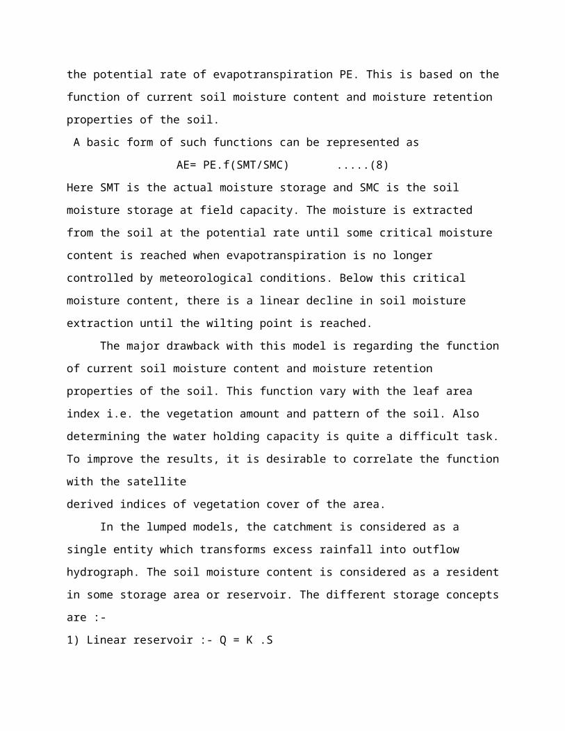
actual rate of evapotranspiration AE and the potential rate of evapotranspiration PE. This is

based on the function of current soil moisture content and moisture retention properties of the

soil.

A basic form of such functions can be represented as

AE= PE.f(SMT/SMC) .....(8)

Here SMT is the actual moisture storage and SMC is the soil moisture storage at field capacity.

The moisture is extracted from the soil at the potential rate until some critical moisture content is

reached when evapotranspiration is no longer controlled by meteorological conditions. Below

this critical moisture content, there is a linear decline in soil moisture extraction until the wilting

point is reached.

The major drawback with this model is regarding the function of current soil moisture content

and moisture retention properties of the soil. This function vary with the leaf area index i.e. the

vegetation amount and pattern of the soil. Also determining the water holding capacity is quite a

difficult task. To improve the results, it is desirable to correlate the function with the satellite

derived indices of vegetation cover of the area.

In the lumped models, the catchment is considered as a single entity which transforms excess

rainfall into outflow hydrograph. The soil moisture content is considered as a resident in some

storage area or reservoir. The different storage concepts are :-

1) Linear reservoir :- Q = K .S

2) Logarithmic reservoir :- Q = K . exp (S)

3) Non-Linear reservoir :- Q = K . S^(1/m)

Here Q is reservoir outflow, S is the storage K is the storage constant and m is the exponent.

These models are usually used for a short period of time like for a day. models for time period

spanning over a month have also been developed now.

3. 3) SPATIAL HYDROLOGY MODELS

These models make use of GIS data structures to stimulate the water flow and transport in a

specified region. These models are used for a variety of operational and planning purposes. It

provides spatial resolution finer than the one that can be provided by observed data. It also gives

great amount of information regarding effects of land use and climate variability and help in

estimating point and non-point sources of pollution leading to the streams.

The current models uses the factors which determine the formation of runoff which include

the topography of the water reservoir, negative exponential law relating transmissivity of the soil

with the vertical distance from the ground level. In these models the total flow is the sum of

surface runoff and the flow in the saturated zone. The surface runoff is also a sum of the water

on the ground surface entering the soil and that generated by saturation excess mechanism.

For these models the catchment area can be divided either into hydrological response units

which are similar with respect to the selected characteristics and which are modeled separately,

or into equally spaced square grid elements. In the first approach the problem that arises is that

the characteristics should be related to hydrological process. If there are a large number of

characteristics, the partitioning will be very detailed and if we consider few characteristics, we

are neglecting the fact that all the water units are different in some aspect. In the second

approach the problem is that the different units will have completely different characteristics and

hence there will be large differences in the modeling of these units.

4) WATER ASSESMENT UNDER CLIMATE CHANGE

The regional water resources are greatly affected by the climatic changes happening in that

region. These water resources affect our day to day life, the changing eater resources have vast

social economical effects. Thus to account for these climatic changes climate models which

simulate climatic effects of the increasing concentration of the greenhouse gases, hydrological

models which simulate hydrological effects of the climatic changes and downscaling techniques

which acts as a link between these two models has been developed.

To project the climate changes, global climate models are used. These models are the type of

general mathematical climatic models of the general circulation of the planetary atmosphere or

ocean based on equations on rotating sphere with thermodynamic terms for the energy sources.

Atmospheric and oceanic models are the key components of the global climatic models along

with sea ice and land surface components. In these models, scientists divide the planet into a 3-

dimensional grid, apply the basic equations, and evaluate the results. Atmospheric models

calculate winds, heat transfer, radiation, relative humidity, and surface hydrology within each

grid and evaluate interactions with neighboring points.

Global Climate Models (GCMs) used for climate studies and climate projections are run at

coarse spatial resolution and are unable to resolve important sub-grid scale features such

as clouds and topography.  As a result GCM output cannot be used for local impact studies. To

overcome this problem downscaling methods are developed to obtain local-scale

surface weather from regional-scale atmospheric variables that are provided by GCMs. Two

main forms of downscaling technique exist. One form is dynamical downscaling, where output

from the GCM is used to drive a regional, numerical model in higher spatial resolution, which

therefore is able to simulate local conditions in greater detail. The other form is statistical

downscaling, where a statistical relationship is established from observations between large scale

variables, like atmospheric surface pressure, and a local variable, like the wind speed at a

particular site. The relationship is then subsequently used on the GCM data to obtain the local

variables from the GCM output.

All these methods consists of these basic steps :-

a) The global climate models are used to derive the parameters which are used for prediction of

future climatic scenarios.

b) These climatic scenarios are further downscaled into local or regional climatic scenarios with

various statistical tools.

c) These are then used to run previously tested hydrological models.

These models don't necessarily predict the future climate changes, they only show how much

hydrological sensitive the system is to the possible climatic changes in that region.

5) CALIBRATION AND VALIDATION OF THE MODELS

After the formation of models, next important step is to calibrate and validate these models.

There have been several methods and tests developed to check these models and make sure

desirable results are achieved. The tests developed follows a hierarchical framework because the

modeling tasks are ordered according to the increasing complexities. In the stationary conditions

simple tests are used while in transient conditions same tests are used along with differential

approach.

In simple split sample test, measured time series data is split into two sets and each of them is

used for testing and calibration. The results from both samples are then compared with each

other. For differential test the data is divided according to some variable which is meant to show

that the model has general validity so that it can predict the value of the output variables for

conditions different from which it is calibrated. The remaining methods remains same.

In proxy basin test, the data is collected from two different basins. This test shows that model

has greater general validity as the model is calibrated against the data of one basin and is

validated against the data of another basin. In differential approach the data is separated into two

sets based on some output variable like rainfall.

In both of the differential models, the models are calibrated against the data for one set of

model and validated for another contrasting set of output variable. For example if the model is

calibrated for a dry season then it should be validated for a wet season. For the distributed

models, the comparison is done according to the data at the specific points which are at the

external boundaries or on the intermediate locations in the grid.

6) PROGRESS MADE BY THESE MODELS

Modeling is perhaps the most accurate way to address the water resource problem and to access

the quantity of the available water resources. These days more and more models are being

developed and used continuously for water resources planning, development, assessment, and

management.

1) Many hydrological analyses uses lumped conceptual models for estimating outflow

2) The use of these models is increasing day by day as the demand for forecasting of future

hydrological conditions resulting from climatic changes is increasing.

3) With the development of technology, new computer simulations can be created to determine

water quality, ecology, risk and uncertainty, environmental impact, etc in addition to normal

hydrology assessments.

4) The data regarding all the water resources