Embed Size (px)
Citation preview

\\ MATHEMATICAL MODELLING AND DESIGN OF A THREE-DIMENSIONAL
GEODETIC NETWORK FOR LOCALISED EARTH DEFORMATION //
by
Sammy Mulei/Musyoka
A thesis submitted in partial fulfilment for the Degree of
Master of Science in Surveying & Photogrammetry
in the University of Nairobi
September, 1993
DECLARATIONS
This thesis is my original work and has not been presented
for a degree in any other university.
S.M. Musyoka
This thesis has been submitted for examination with my
approval as University supervisor.
(ii)

ABSTRACT
Mathematical models, within the framework of integrated
geodetic networks for localised three dimensional geodetic
men i ter ing networks are presented. The network design aspects have also been considered.
The development of these mathematical models was based on the
kinematic estimation model of geodetic network adjustment
using the integrated geodetic approach. The network design
aspect considered was the weight problem for each of the
various observables used. These observables were astronomic
latitude, astronomic longitude, astronomic azimuth, vertical
angles, horizontal directions, spatial distances, gravity
differences and gravity potential differences. The basic
parameters computed were the network coordinates, the point
velocities and accelerations of the unstable points.
In order to test the validity of these mathematical models, a
test network consisting of six points, derived from an old
map of Olkaria Geothermal station in Kenya, was used. One of
these points was intentionally shifted so as to cause network
deformation. Five epochs of observations were considered;
with a uniform epoch interval of one year. The adjustment of
the initial network was carried out on the basis of a free
network, whereas the rest were computed as fixed. The
numerical study was entirely carried out by computer
simulation.
( i i i )
Through the models adopted it was possible to estimate both
network coordinates and point velocities of the object
fieuwor*\ with a u least two epochs of observations while
accelerations required at least three observation epochs.
These requirements were in line with the theoretical aspects
of the models. The estimated velocities were consistent with
the shifts that were introduced into the network.
Tne results also showed that a small proportion of astronomic
azimuth observations were needed while gravity differences were not required.
( i v )

ACKNOWLEDGEMENTS
I wish to express my deep gratitudeto my supervisor
Dr.-Ing. F.W.O. Aduol, for his advicece’ encouragemeot «nd
suggestions which have greatly contributed toward, completion of this thesis.
I am also indebted to the Board of Postgraduate studiej without whose scholarship I would not have been
pursue this course. Further thanks go to the beans Committee]
University of Nairobi, for generously funding the thesis, and
the University of Nairobi in general for offering me
appointment as Graduate Assistant which enabled me to pursue
the second part of my MSc. programme as a member of staff in
the Department of Surveying & Photogrammetry.
I would also like to acknowledge the assistance of Prof. (».
Schmitt of the Institute of Geodesy, Karlsruhe and Prof w.h,
leskey of Dept, of Surveying Engineering, University of
Calgary, who so kindly supplied me with some relevant
literature. I also extend my thanks to Mr. Mwangl,
Geophyscist at the Olkaria Geothermal Power station, who
supplied me with the maps for that area.
I am also grateful to the staff of the Department of
Surveying & Photogrammetry, Universtiy of Nairobi, who
been very cooperative during the time I was preparing ,h'R
thesis. To my collegue , Mr. J.B.K. Kiema, I very thankful J
for his suggestions and criticisms that he offered me.
Finally, I am grateful to the staff of the Inst1was so helpful
Computer Science, in particular Mr. Mungai w
during the computation period.
(v)

TABLE OF CONTENTS
PageDECLARATIONS (ii)
ABSTRACT (iii)
ACKNOWLEDGMENTS (v)
LIST OF FIGURES (x)
LIST OF TABLES (xi)
1. INTRODUCTION 1
1.1 The statement of the problem 2
1.2 State of the art 4
1.3 Organization of the report 6
2. ESTIMATION MODELS FOR LOCAL DEFORMATION MONITORING
2.1 General models 7
2.1.1 The simple Gauss-Markov model 7
2.1.2 The simple Gauss-Markov model with exact
restrictions 8
2.1.3 The free network adjustment model 11
2.2 The Integrated model 12
2.3 Estimation Models for Deformation Monitoring
2.3.1 General models 13
2.3.2 The simple kinematic model 16
2.4 Concluding remarks 20
3. THE LOCAL THREE-DIMENSIONAL GEODETIC MONITORING
NETWORK MODEL
3.1 Coordinate systems 23
3.1.1 Curvilinear physical coordinate systems 23
3.1.2 Local astronomic coordinate system 24
(vi )

( v i i )
3.1.3 Ellipsoidal cartesian coordinate system 24
3.1.4 Ellipsoidal curvilinear coordinate system 24
3.1.5 Local ellipsoidal coordinate system 25
3.1.6 Geocentric cartesian coordinate system 25
3.2 Coordinate Transformations 27
3.2.1 Rotation matrices 27
3.2.2 Transformation between geodetic cartesian
and ellipsoidal curvilinear systems. 28
3.2.3 Geocentric and local astronomic
coordinate systems 28
3.2.4 Geocentric and ellipsoidal cartesian
systems 29
3.2.5 Ellipsoidal cartesian and the ellipsoidal
local systems 30
3.3 The Observation Equations 30
3.3.1 Gravity potential 31
3.3.2 Gravity intensity 34
3.3.3 Astronomic latitude 36
3.3.4 Astronomic longitude 36
3.3.5 Astronomic azimuth 37
3.3.6 Vertical angle 40
3.3.7 Spatial distance 42
3.3.8 Horizontal direction 44
3.3.9 Gravity potential difference 45
3.3.10 Gravity difference 46
4. THE MONITORING NETWORK
4.1 The test network 48
4.2 Simulation of observations 48
4.3 Weighting of the observations 51
A m 3 . 1 Gravity potential differences b1
t 3 . 2 Gravity differences ^
3 . 3 Astronomic latitudes b;,
3 . 4 Astronomic longitudes b;,
3 - 5 Astronomic azimuths b 4
3 . b Vertical angles b3
3 . 7 Spatial distances b3
. 3 - « Horizontal directions b4
.4. T he computer program for simulation of
observations 54
. t> Elements of the deflection of the vertical 55
. e> I h e free network solution 56
M t N E T W O R K DESIGN AND COMPUTATIONS
. 1 Introduction 53
. ^ N e t w o r k simulation 60* ^ * 1 1 he variance component estimation 61* * 2 1 he design layout 63
1 h e precision criteria 64■ s - 1 Positional standard errors 65^ * z Spherical standard error and spherical
probable error 65- 0 Mea n radial spherical error 65^ standard error ellipsoids 66
Concluding remarks 664 I L
'e results of computations for initiale P o c h 67
X ' 1 T EST I 67* * ^ T EST II 71s
D ° c h 11 results 73D ° c h III results 74
/ «D o c h IV results 75

(1x)
5.8 Epoch V results
5.y Ihe Main Computer program
DISCUSSIONS 82
CONCLUSION
7 .1 Summary
7.2 Conclusions
7.2 Recommendations
8b
86
87
88
APPENDICES
A. THE PARTIAL DERIVATIVES USED IN THE
OBSERVATION EQUATIONS. OQ8 9B. PROGRAM FLOW CHARTS.
B .1 The data simulation program (SIMUL) 91
B. 2 The main program for adjustment (ADAN) 92
c. PROGRAM LISTINGS AND THE RESULTS.
c.l Program listing for the data simulation Program (SIMUL) 94
C. 2 Program listing for the Main program (ADAN) 99
C.3 Results of program ADAN for 2nd to 5thepochs
132C.4 Results for the 5th epoch of
observations- static mode
148REFERENCES

( X )
LIST OF FIGURESFigure 2.1a
Figure 2.1b
Figure 2.2
Figure 3.1
Figure 4.1
Minimal constraint adjustment.
Overconstrained adjustment.
The parameters computed in a kinematic
estimation model for five observation
epochs
The geocentric cartesian and ellipsoidal
coordi nates
The sketch of the network
1010
21
26
49

(xi)
LIST OF TABLES
I able 5.1 lhe simulated observations of the full model 68
lable 5.2 Approximate coordinates 70
table 5.3 1 he fully observed network 70
lable 5.4 The estimated coordinates for the full model 71
lable 5.5 The parameters of the error ellipsoids for the full model 71
Table 5.6 The optimised network 72
Table 5.7 The estimated coordinates of the optimised network
Table 5.8 The parameters of the error ellipsoids for the optimised network 73
Table 5.9 Results of epoch II observations 74
lable 5.10 Results of epoch III observations 75
Table 5.11 Results of epoch IV observations 76
Table 5.12 Results of epoch V observations 77
Table 5.13 Estimated coordinates for Epoch V
(fixed mode) 77
lable 5.14 The fifth epoch free network results 78
Table 5.15 Estimated coordinates for Epoch V
observations (free network mode) 78
Table 5.16 The parameters of the error ellipsoids
(free network) 79
CHAPTER ONE
INTRODUCTION.
It is a well known fact that certain types of terrain are not
at rest, but are slowly moving, thereby causing positions < f
points located on them to change. Some of the factors causing
these movements are crustal deformations, volcanic activity
variation of ground water level, mining activities, and
construction of large engineering structures.
Generally, the deformation may be classified into two types:
crustal and localised earth deformations. Crustal earth
deformations take relatively long periods of time to show any
appreciable ground shifts, whereas localised earth
deformations tend to be of relatively short frequency so that
they can be noticed in much shorter periods of time. Factors
contributing to localised earth deformations include
engineering construction works and mining. As a safety
measure, and also as a guide for future planning in a given
area suspected to be unstable, the deformation of the ground
need to be monitored as to seek to detect any deformations
thereof.
There are various ways of monitoring earth deformations.
These include geodetic techniques as well as photogrammetr 1 <
methods [e.g. Shortis, 1983], Of these methods, geodetic
methods of monitoring earth deformations have found wide
application because of the advantage in that they al ow
monitoring of relative movements to very high accuracie*t- o be[Ashkenazi, 1980]. These methods have however began
applied more extensively in the last few years as reported
[Cooper 1987], In this study it is aimed to make a furthe
1

^he neglection of the influence of certain systematic
effects on the parameters such as deflection of the vertical,
particularly in mountainous regions [Grafarend, 1988],
refraction influences and effect of variation of the gravity
field in general may significantly distort the network. Also
the deterioration of azimuth within the network should not be
i gnored.
To overcome these difficulties, a three-dimensional
adjustment should be adopted to provide a system of precisely
coordinated points in three-dimensional space, in line with
the observational model. For a three dimensional adjustment,
observations need not be directly transformed into the
reference ellipsoid, and the azimuths are controlled
implicitly.
In order to facilitate the computation of a rigorous three-
dimensional network, the quantities that would ordinarily be
observed comprise horizontal directions, angles, spatial
distances, vertical angles, astronomic latitudes, astronomic
longitudes, astronomic azimuths, gravity potential
differences and gravity intensity differences. All these
observations are incorporated into a single adjustment
process within the physical gravity field in which they will
have been measured. For each station the three coordinates,
either in cartesian coordinate system or the curvilinear
system, are obtained together with the deflection of the
vertical parameters. Other auxiliary data such as the
refraction coefficients are also estimated.
Following the above discussion, this study will principally
aim at setting up suitable mathematical models that would be
needed for the establishment of a three-dimensional geodetic
network for the monitoring of localised earth deformations.
3

Further, a simulated network will be designed for the
purposes of demonstrating the pertinent mathematical models.
1.2 State of the Art.
Deformation measurements and the analysis of movements are an
essential task in the field of engineering. Considerable work
done so far in deformation surveys has been reported ’ in the
'-i\.ceeJingo of the Symposia on Deformation* (Commission
6-Engineering Surveying of the International Federation of
Surveyors, FIG). Since the establishment of this Commission
by FIG, the subject has received considerable contributions
from various authors. Some of the publications which
addressed the problem of detection of deformation were by,
amongst others, van Mierlo ( 1975), ( 1975a), Brunner( 1979 ),
Niemeier(1931), Koch et al (1981), Chen et al (1983), van
Mierlo(1981), Pelzer( 1977), Ashkenazi et al ( 1980), Chen et
al (1930). A number of geodetic monitoring networks have been
established on the basis of principles discussed in these
papers.
Kelly (1933) reports on the monitoring surveys at Loy Yang
(Australia) while Murnane( 1983) details the aspects of
network design and analysis at the Winneke reservoir
(Australia) monitoring surveys. Crosilla et al (1986) report
on a study carried out to monitor current crustal
deformations in a local area (Friuli) in Italy. Relative
gravimeter observations for monitoring vertical motions along
the Boccono Fault in Venezuela have been described by Drew
(1989). Recently, Biacs et al (1990) prepared a PC-based
program system for adjustment and deformation analysis of
precise engineering and monitoring networks, which they
successfully applied on the Paddle River surveys and the
Olympic Oval monitoring network in Canada.
4

In deformation monitoring, it is generally assumed that
measurements can be made very quickly with respect to the
speed of deformation and that these measurements are made at
an epoch (instant of time). When this assumption does not
hold, then time factor must also appear in the model as a
fourth parameter. Papo and Perelmuter (1984) suggested
inclusion of velocities and accelerations of points in the
functional model. Aduol and Schaffrin (1990) extended on the
idea of inclusion of velocities and accelerations to the
kinematic model of deformation monitoring.
To this end, deformation is defined not only to mean change
of shape but also to include scale changes, rotations and
shifts. In using geodetic networks to monitor deformation,
the deformation parameters are derived from changes of
coordinates that might have taken place. Unfortunately, the
coordinates are datum dependent and the choice of fixed
reference datum may be hard to obtain. If one is able to
identify some points as fixed and retain their coordinates at
every epoch of observation then this is called an absolute
monitoring network. If on the other hand, all points in the
network are likely to undergo deformation, then this is a
relative monitoring network. Since no points in the
monitoring network can be said to be stable unless
measurements confirm it, then the adjustment must be carried
out on the basis of free network [Chen et al ,1990].
The free network adjustment has been discussed in various
publications. These include Grafarend and Schaffrin (1974),
Perelmuter (1979), and Mittermayer (1972). One advantage of
free network analysis is that no point is kept fixed, and the
datum is defined through the approximate coordinates of the
proposed network.
5

The idea of computing a geodetic network in three dimensions
may Le attributed to Bruns, who suggested the computation of
a triangulation net in space in 1878 [Heiskanen & Moritz,
1967]. More studies followed later and it was shown that most
of the problems encountered in adjusting separated networks,
such as reduction of observations onto the reference spheroid
could be avoided. Aduol(1981) in his study on optimal design
of a three dimensional geodetic network based on simulated
data observed that among the commonly observed values of
vertical angles, distances, horizontal directions
respectively angles, must also be included one each of
astronomic observations of azimuth, latitude and longitude.
Also with inclusion of gravimetric data, the number of
astronomic positions could be reduced. Observation equations
for computation in three dimensional in integrated networks
are presented in [Aduol 1989].
1.3 Organisation of the report.
In Chapter Two, the theoretical aspects of the parameter
estimation models are discussed. Presented in Chapter Three
are the necessary observation equations that were used in the
adjustment process. The various coordinate systems that are
required in the study together with their transformations are
also discussed.
The network simulation and results of simulation are
presented in Chapter Four. In Chapter Five are presented the
computations and the results of these computations. The
results are discussed in Chapter Six and major conclusions
made in Chapter Seven. The notation used here is defined in
the text of the report.
6

CHAPTER TWO
ESTIMATION MODELS FOR LOCAL DEFORMATION MONITORING.
2.1 General Models.
Hor the estimation of the unknown parameters, the linear
least squares model is here adopted. The general basis for
this estimation will be the simple linear model commonly
referred to as the simple Gauss-Markov model. In the
following sections we shall therefore consider the estimation
of the parameters under the simple linear model as the basic model .
2.1.1 The Simple Gauss-Markov Model.
If A be an nxu matrix of known coefficients and of full
column rank, x a ux1 vector of unknown parameters to be
estimated, y an nx1 vector of observed values, then the
simple Gauss-Markov model may be represented in the form
y = Ax + £ ; D(y) = <y2 W~1 = D(r ) = 0, (2.1)y O yy y
for e being an nx1 vector of observational errors, W is ay yy
known nxn positive definite weight matrix of the observed
values in vector y and o is a variance component (also
called variance of unit weight) of the observations. TheA
least squares estimate of x , x can be shown to be
x = (A’WA) 1A ’Wy , ( 2 .2 )
with
D(x) = o“~ ( A ’ WA ) 1 - • V (2.3)
and also
E[x] = x (2.4)
7

From (2.4), it is noted that x is an unbiased estimate of x.
In fact it can be shown that x is the best linear unbiased estimate of x.
Ihe simple linear model under the Gauss-Markov model requires
that the normal equation matrix has full rank. In case of
rank deficiency, which is usually the case with survey
networks, it has to be overcome in some way.
2.1,2 The Simple Gauss-Markov Model with exact restrictions
One way to overcome the rank defect in the Gauss-Markov model
defined in equation (2.1) is to set up some exact
restrictions in the form
r = R x , (2.5)
where R is a cxm design restriction matrix while r is a cx1
vector of restrictions.
Grouping equations (2.1) and (2.5) in matrix form, one obtains
y A £X + y
_ r _ _ R _ _
The next step is to minimise the quadratic norm, s'Ws undery y
the restriction (2.5). The Lagrange function L is formulated
thus
L = c ’Vte - 2X(Rx - r) (2.7)y y
where X is a cx1 vector of Lagrange multipliers. The system
of the normal equations matrix then takes the form:
8

m; therefore toThe rank of A is q < m while that of R is c
ma^e N regular the restrictions are incorporated as
N = N + R * R . (2.9)
The inverse of the normal equation matrix is obtained from
[e.g Schaffrin, 1984] or in [Aduol 1989] as
-1Ni R *
tF F 11 12
R 0 OJLl_OJlL___
1
with11
r N 1- (N V ) ( R N 1
F1 2- (N ‘r ’ h r n 'r * )'*
F2 1 = (RN*R’ ) ‘r n' 1 = F
F22 = I - (RN 'R ’) ‘
andx = F A ’Wy + F r 11 12
D(x) : r F A ’WAF ’XX Oil 11
(2.10)
(2.11a)
(2.11b)
(2.11c)
(2.11d)
(2.12a)
(2.12b)
In a survey network these restrictions may take the form of
fixed control points used to coordinate new points. In this
case the quality of the network deteriorates further away as
the new points are separated from the control points as shown
in Figures 2.1a and 2.1b [Niemeier, 1985], for a two
dimensional network. From these two figures, it is noted that
the distribution of the control points must be chosen
9

Fig. 2.1a Minimal constraint adjustment. The fixed points are 1 and 3 (after [Niemeier, 1985])
Fig 2.1b Overconstrained adjustment. The fixed points are 1 3 and 11 (after [Niemeier, 1985])
10

2.1 .3. The J^ree network adjustment model.
The free network adjustment resulted from the principles of
Meissl’s Inner Error Theory [Meissl, 1962, 1969] in Meissl
(1932) and also advocated by others. It is shown [e.g.
Mittermayer, 1972] that under free network adjustment, in
addition to the least squares condition that the quadratic
norm ^ ’W be a minimum, that one of the conditions
carefully. The control network should also be of highprec is ion.
x'x = minimum or (2.13)trace(D(x ) ) = mini mum, (2.14)
be imposed on the network. From equations (2.13) and (2.14)we have that neither the length of the correction vector nor
the sum of the variances resulting from a free network
adjustment can be improved any further by a change of origin,
orientation or scale. One is thus justified to define a free
adjusted network as a network with the best reference datum.
The basic linear model is of the form shown in equation (2.1)
and a restriction of the form (2.5) is set up in the solution
of a free network so as to overcome the rank defect. The
choice of the restriction design matrix is made such that R
will be a matrix whose columns are made up of the normalized
eigenvectors of those eigenvalues in the normal equations
matrix which have values equal to zero due to rank defect in
N [e.g. Aduol, 1990]. Usually, R is denoted by G and has
properties that
NG = 0 (2.15)
G ’G = 0 (2.16)
The constraint equation for adjustment of a free network is

G ’ x = 0Various forms of the G matrix for different observation and
network types have been listed by I liner ( 1985). For a
three-dimensional case in which horizontal angles have been
observed (i.e defects = 7), G is of the form
( 2 . 1 7 )
1 0 0 1 0 0 ___ 0 00 1 0 0 1 0 __ 1 00 0 1 0 0 1 ....... ....... 0 0 10 zl -Yi 0 zl - Y .......i zl -Y i
- zi 0 Xl -zt 0 X .......1 . . . -zl 0 X
iYi -Xi 0 Yi -Xl 0 ....... l -Xi 0X Y z X Y z ....... Y zi i l t i 1 l i l
(2.18)
If distances be observed, the seventh row is deleted since
observed distances control the scale of the network.
Similarly, if azimuth observations be made then the fourth,
fifth and the sixth rows are deleted. It is here mentioned
that the final coordinates, but not the shape of the adjusted
network, depends upon the provisional coordinates.
Noting that the normal equation matrix N is singular, the
problem of adjusting for free networks becomes principally
one of overcoming the rank defect in N. Several approaches to
the solution of N have been suggested by, among others,
Grafarend and Schaffrin (1974), Perelmuter, (1979); Cooper,
(1980); Brunner, (1979); Chen et al (1990) etc. The main
approaches are through the use of generalized inverse
matrices and the similarity transformations.
2.2 The Integrated Model
The integrated adjustment models involve both geometrical
12

observations and gravity field data. Reference to integrated
models is made to Grafarend and Richter (1978), Grafarend
- 3), Aduol (1989) and others. In most usual surveying
practices, one uses the geometrical observations of
distances, horizontal directions or angles and vertical
angles to solve for the network without regard to the
direction of the plumbline at each network station. The
integrated models incorporate gravity data into the
adjustment to allow computation of the directions of the
plumbline at the network points together with other
parameters.
The basic equation in an integrated adjustment model may be
represented in the form
Y = f(X ) + f ’(X)£X + 6 f(X ) + t (2.19)O Y
where Y is a vector of observables, f(X ) is a vector
representing the values computed using the model function and
< X is a vector of the corresponding parameters. The vector
f(X) is the vector of disturbances, such as the deflection
of the vertical parameters. The vector c is the vector of~Yrandom errors in the observable vector Y.
2.3 Estimation models for Deformation Monitoring.
2.3.1 General Models
One approach to the analysis of repeatedly measured networks
to detect movement is to estimate individual coordinate
vectors for each epoch. The functional model of this set is
[Niemeier, 1981]
13

i<<l5. rxi £1 11 12 .....................Ik i l
y ! A A A X £2 = | 21 22 2k 2 + 2• • ;
y. 1 A A A X £L kJ [Jk1 k2 kk k k
with y being an (n ,1) vector of observations, r an (n ,1)1 «> i i
vector of residuals, A an (n ,u ) coefficient ofij i i
configuration matrix, x is a (u ,1) vector of estimates fori ithe parameters of the network, e.g. coordinate points, n is
the number of observations in the i-th epoch, u is theinumber of parameters in the i-th epoch and k, the number of
epochs. The stochastic model is given by
10 Q .Q , 111 12 ik j„ 2 2 Q Q QK - Cf Q = a 21 22 . 2k
VC VC 0 VC VC 0
11 •
Q Q QCM kk
( 2.21 )
with kyy
as the variance-covariance matrix for the
observation of all epochs; a is the variance of unit weight,cvalid for all epochs; Q is a cofactor matrix of the
yyobservations of all epochs; 0 , is a cofactor matrix
i-Jcorresponding to the observation vectors y and y .
J
The main solution for each epoch is given by [e.g. Brunner,
1 979]
x = (A’Wa T A ’Wy
Q+ = ( A’ WA)xi
(2.22a)
(2.22b)
where + indicates the
[Bjerhammar, 1973]. This solution
cofactor matrix of minimum trace;
Moore-Penrose inverse
has minimum norm and a
in fact it is a free
14

To detect whether any motion has occurred between the epochs,
the global testing is carried out by computing the variance of unit weight.
The estimation for the variance of unit weight o2 , which is a
global quantity for the accuracy of the epoch is computed as
network solution as described in the previous section.
£ ’Wc2 i iO - ----n-u(2.23)
The hypothesis,
H : E lo2 ] = E (p ] = ......... E [o'2 ]o o i o2 ok
H : E [■/ ] * E \tj ] * ......... E [</ ]A o I o2 ok
(2.24)
(2.25)
may be set up. If the hypothesis H is accepted, then the
conclusion may be that no movements of the station
coordinates have occurred.
A better estimable quantity for the precision of the epochs
being compared is obtained if one sums up the single
quantities of each epoch [Grundig et al, 1985, Niemeier,1981]
c: ’We + £ ’We;2 _ »• »■ j )
— --------------o r + r
*• J(2.26)
with r + r being the degrees of freedom.1 2 * 2This computed value o corresponds to a common adjustment of
the two epochs in which the variables of one of the epochs
are not considered identical to those of the other epoch.
A deformation vector d, for any pair of observation epochs
consisting of coordinate differences, can be set up as
d = x.- x (2.27)i J
15

The quadratic form d ’Wd, and the quantity Q2
for the purpose of testing the validity
conditions [Grundig et al , 1985].
can be computed
of the assumed
d ’W dQ2 = - dd (Q + Q )+
1 J (2.28)
with h = m-r^, with m being the number of conditions r , is
the rank deficiency of the variance-covariance matrix. The 2 2
quantities 0 and o are both statistically independent
[Grundig et al 1985] and can therefore be tested against each
other. The test statistic given in Grundig (1985) is
If
♦F =
the quantity F♦
A 2Cfofits the Fischer
(2.29)
distribution, i.e.
P(F*< Fl -Qt , f 1 , f 2 1 -a
1-a = level of significance fi = h and f2 = r + r are degrees of freedom,
then the null hypothesis is accepted.
(2.30)
2.3.2 The Simple Kinematic Model
Reference to the simple kinematic model is made to [Aduol and
Schaffrin 1990]. The basic concepts of this model are
discussed here below.
Let us take G to be the function relating the geometric and
the physical parameters (x , x ....... x ) so that the1 2 krelationship is represented as G(x , x ....... x ). For a more
1 2 kgeneral case, let the function G at epoch i be nonlinear soithat linearising it about a point, one writes
16

G (x , x . . ., . . x ) = G (x . x . .X 1 fx x ...x )2 ».1 2 P G L 1 2 • i
(2.31)simplified as
Gi — G + uGO'. t (2.32)wi th
0 G OG OG«~G = — Ox - L,x + r-- 4-.X +. . .1 Jx 2 + -- AxOx (2.33)
i 2 iCand
x = x + Axi O l V
x is the approximate value for xO '. L and ^x is the smallcorrection due to nonlinearity of G.
Introducing a time factor in equation (2.31), and consi dering
the initial epoch of observation to have been made at a time
t =t i.e aftert i At =t -t has elapsed,i i i then the relationship
G at the i-th epoch, may be obtained from the function G as
G G + 1 0' G
2 Otf(2.34)
after considering up to second order terms. To estimate the
point velocities and accelerations, one sets the partial
derivative of the displacement with respect to time and
manipulates the result as follows:
and
OG OG Ox. iOG Ox . 2+ ..... ... ... + . ,. . +
OG
01 X dt Ox <>t 2 i)xk
Ot
17

d' G _ <) I dG !I —- i — ■■■ |dt d1 ( <>t )
d f dG dx dG dx d G dx }- --- t --- t +-- * 2
--- + . . . + • k 1— idt ( dx l dt dx2 Jt <)x
jC at J
OXwhere --- represents the coordinate velocity and
dt
(2.35)
i --- idt ( dt J
is a coordinate acceleration.
Now,taking into consideration that G is nonlinear (for aigeneral case) then (2.34) would be rewritten as
_ ^ ’ i- a +i
• >G
dxx +i
oxX +
2
dG
dx
f dG dX dG dx. 1 . 2
( dx dt dx c)t2
dG dx 'j+ . . . + --- --- ' ut
dx dt J
« f dG d x11 . i+ 2 ( dx dt1
dG d x+ . . . +
dx2 dt
OG d x
dx dt
(2.36)
One then considers the vector of the observation G so thattG. =E[G. ]. Associated with this vector is the observationali verror e. so that E[£.]=0. These vectors can be represented
i ias
G - G + £i i(2.37)
using the notation
18

• *' x J X 'j
x ’ <>t • x = <Tt(Jt J
to represent the velocity and acceleration respectively
Equations (2.36) and (2.37) may be related as,
0« _ u. ~ u . -1 0 i
oG—--- LA X +O X I
<*G
z. + +
dG . .+ -r— ^t X +OX i 1 1
dG .T at X + . . .ox ». z 2
dG . .+ -r- iit X +
<>x i kV
1 JG .2 ..— t X +2 i)x i l1 OG 2 . .-r-T ot X +2 dx i 2
1 <>G
+ £• (2.39)
Equation (2.38) is the general linearised observation
equation for the kinematic estimation of the parameters.
In the kinematic estimation model, one is able to estimate
the network coordinates during the initial epoch. During the
next epoch of observation (i.e the first epoch) this model
can estimate both the network coordinates and the point
velocities. A second observation epoch would enable
estimation of network coordinates, point velocities and point
accelerations. More observation epochs would strengthen the
estimation of the above parameters. A diagrammatic
representation of this hierarchical estimation of parameters
is shown in Figure 2.2. From the theory of this estimation
model, the network coordinates are referred to the initial
epoch observations (i.e they do not change). Any movements
are detected implicitly through the estimated velocities.
19

2.4 Concluding remarksThe simple Gauss-Markov model of section 2.1.1 requires that
sufficient points of the network be known a priori and
absolutely in order to solve for the network. In a monitoring
case, only the object network can be solved in this manner
assuming that the reference points used are taken to be of fixed.
i fie estimation model 2.1.3 of free network case seems
favourable for solution of the reference network as no
network points need to be known a priori. It would also seem
favourable to adjust the object network on the basis of a
free network defining the datum over all points of the
reference network.
20

' 1 -----------------------I' I
iEPOCH 1 POSITIONS
I I |j j t i; EPOCH 2'i •i i POSITIONS
1 1
VELOCITIES
1i! EPOCH
fi
3; POSITIONS VELOCITIES
------r ■ ■ .. — ■ ■
.1 ACCELERATIONS
i
! EPOCH
»
4 :
1
♦POSITIONS VELOCITIES ACCELERATIONS
11
1 EPOCHj
j5 i
Jt
POSITIONS VELOCITIES
Ii
1 ACCELERATIONS{1 . !
Fig 2.2 The parameters
model for five
computed in
observation
a kinematic estimation
epochs.
21

-he integrated model of adjustment discussed above seems
favourable in those areas where the earth’s gravity vector
(respectively plumb line) is greatly varying. Such are areas
of varying terrain (mountainous regions) and also mining
zones. And again for computation of heights derived from
vertical angles, the direction of the plumb line should be
known.
'he general models of section 2.3.1. provide information on
whether a network has moved or not between two epochs of
observation. If the network has moved, then one is required
tc carry out a further analysis to detect the particular
points that have moved and also to find the magnitude of
displacement.
The simple kinematic model provides complete information on
the analysis of a monitoring network: the unstable points are
identified by the speed of movement and the acceleration is
also estimated explicitly.
Putting into consideration the above discussion, the present
study adopts the kinematic estimation model using the
integrated approach for the solution of a monitoring network
for localised earth deformation monitoring.
In monitoring networks where more than one epoch of
observations have been made, we note that we are able to
estimate not only point positions but also the point
velocities and accelerations. The kinematic estimation
incorporating the integrated model therefore seems a more
suitable estimation model where more than one epoch of
observations are made. This approach is adopted in this
study.
22

CHAPTER THREE
THE LOCAL THREE-DIMENSIONAL GEODETIC MONITORING NETWORK MODEL
3.1 Coordinate systems.
The coordinate systems that are discussed in this section are
those that are relevant to coordination of geodetic network
points in three dimensional space. These are astronomic,
geocentric and ellipsoidal coordinate systems.
3.1.1 Curvilinear physical coordinates.
This system consists of the astronomic latitude $, astronomic
longitude A and the orthometric height, H which is a function
of the gravity potential W. The orthometric height H is the
geometric distance from the surface of the geoid to the point
P^ of observation, measured along the gravity vector. The
gravity potential W from which H is derived is expressed as
W = Gf f f— (X , Y ,2 )dX dY dZ + -o>2 (X2 + Y2 ) (3.1a)J J J r a a a a a a 2
with ________________________________
r = /[(X-X )2 + (Y-Y )2 + (Z-Z )2]' (3.1b)a a a
where P(X ,Y ,Z ) are the coordinates of the attracting pointa a aand P(X,Y,Z) are the coordinates of the observation point, p
is the density of the attracting material whereas G is the
gravitation constant and a) the angular velocity of the earth.
The orthometric height H is obtained from
(3.2)
w rg
in which W is the gravity potential at the geoid and W , theg P
gravity potential at the standpoint, r is the gravity
intensity along the vertical through point P..
23

3.1.2 Local astronomic coordinate system
The observation point is the origin for this left-handed
system. Denoting the three axes by X , Y* and 1 with the. * * «
corresponding base vectors E , E and E respectively. a* 1 2 3
positional vector R in this system may be represented as
* * * * * * *R = X E + Y E + Z E1 2 3 (3.3)
3.1.3 Ellipsoidal cartesian coordinate system
The origin O of this system is the centre of the reference
ellipsoid. The three axes, x,y,z are orthogonal and form a
right-handed coordinate system. The corresponding base vectors
are V V VThe axis z coincides with the semi-minor axis of the ellipsoid
and is positive in the direction of north.
The axis x is directed such that it passes through an adopted
origin of the ellipsoidal equator. The plane xOz would be
oriented to be as nearly parallel to the Greenwich meridian as
possible.
The axis y completes the right-handed system and is taken
positive eastwards.
3.1.4. Ellipsoidal curvilinear coordinate system.
The three coordinates are ellipsoidal latitude , ellipsoidal
longitude \ and ellipsoidal height h.
The ellipsoidal latitude is the acute angle formed between the
the iellipsoidal equatorial plane.
geodetic normal at the observation point P.. and
The longitude \ , is the angle formed between ellipsoidal
24

meridian through P anc the plane containing the first and the
third base vectors.
The ellipsoidal heignt h is the distance of the point from the
ellipsoidal surface as taken along the ellipsoidal normal. It
is reckoned positive towards the zenith. Refer to Figure 3.1
3.1.5 Local ellipsoidal coordinate system *
The point of observation P is the origin with the axes x* y* *z being orthogcna7 and left-handed. The corresponding base
• • •vectors are e , e , . A positional vector r, in this system
is represented as
* • •r = x e + y e * z e (3.4)
1 2 3
*The axis z is taken along the geodetic normal with the
positive direction outwards from the reference ellipsoid.
*The axis x is in the meridian plane and points 1n the
direction of north.
*The y axis ccwcletes the left-handed system and points in the
direction of east. See Figure 3.1.
3.1.6 Geocentric cartesian coordinate system.
This is a right-harded cartesian coordinate system whose
origin 0 is at the centre of mass of the earth. The three
axes, designated X,t,Z have the corresponding base vectors
F ,F ,F . A positional vector R in this system is represented1 2 3
by
R = XF + YF ZF (3.5)1 2 2
The Z axis of this system points towards the mean north pole
as defined by the Irtemational Polar Motion Service (IPMS).
25

Figure 3.1 The geocentric cartesian and ellipsoidal coordinates

The X axis is in the plane ZOX and is parallel to the
Greenwich Meridian. The Y axis completes the right-handed
system and is positive eastwards. See also Figure 3 .1 .
3.2 Coordinate transformations
The transformation of these coordinates from one system to
another is of interest in this study because of the
requirement of the various mathematical models in different
computation systems. The transformation of the coordinates is
facilitated by use of rotation matrices. These are discussed
below.
3.2.1 Rotation matrices
In coordinate transformation, usually one coordinate system is
rotated into the other through anticlockwise angular shifts ce,
/?, y about the first, second and third axes respectively,
through the rotation matrices
1 0 0
R 1 = 0 cos(oi) sin(o) (3.6a)
| 0 -sin(c<) cos(ot)
cos(^) 0 -sin(f3) ~
R2 = 0 1 0 (3.6b)
_ sin(/?) 0 cos(/3)
cos(y) sin(^) 0 I
X COII -sin(y) cos(^) 0 (3.6c)
0 0 1 J
where R ^ a ) denotes a rotation on the base vector of the first
axis through angle a, R (f?) and R (^) respectively denoteWsimilar shifts through angles (3 and y about the second and
27

third base vectors.
If all the three rotations about the base vectors are carried
out as
= r3<^ )R2<^ >r 1 (a ) (3.7)the resulting matrix is the Cardanian rotation matrix. If on
the other hand, we carry out the following transformation,
R (3.8)o <3 £ O
then we have the Eulerian rotation matrix. The modified
Eulerian rotation matrix in the form
R = R3(r)R2(*/2 -/?)R3(a)
is also used.
(3.9)
3.2.2 Transformation between geodetic cartesian and
the ellipsoidal curvilinear systems.
The relationship between these two coordinate systems are
common [e.g .Aduol,1989]
x = ♦ h"1
V /4 2 . 2 ,(1- e sin ?)C OS £ > C OS \
y =a
♦ h“I
V, « 2 . 2 ,(1-e sin p )cos^s ir\\
(3.10a)
(3.10b)
z =a(1 -e" )
i , . 2 . 2 ,(1 -e sin p)
+ h ! s i np (3.10c)
l _ ' ’ --------------r ' _J
The reverse relationship may be found in Cooper (1987).
3.2.3 Geocentric and local astronomic coordinate systems
This transformation is given as [e.g.Aduol,1989]
28
(3.11a)
r E* " F1 l*E = R (A,4,0) F2 E 2*E3 1
mIL
_____1
where
R_(A,*,0) =
L
si rtf cosA
- s i nA
cost cosA
sirtf sinA
co&\
cos$s i nA
-coat
0
sirtf
(3.11b)
LIThus considering two points P (X* Y * Z * ) and P (X* Y * Z # ) andX X X x J J J Jdefining
* * #
* * *
then the corresponding quantities in the geocentric system may
be obtained from
X*
__1
r x i♦
Y = R (A ,4 ,0) Y♦
Z _i
E
IJ Z
(3.11d)
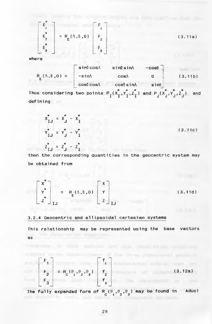
3.2.4 Geocentric and ellipsoidal cartesian systems
This relationship may be represented using the base vectors
as
r f1 1
F = R (3 ,3 ,3 ) f2 C 1 2 3 2
F . fL 3 J 3
The fully expanded form of R ('3 ,3 ,3 ) may be found in Aduolc 1 2 3
29

(1989). Usually the rotation angles are very small so that the
following rotation matrix results
R . * . * > C 1 2 3
l~ 1 e3 2\-e 1 &
3 11
L 2 1
cartesian and
J
(3.12b)
3.2.5 Ellipsoidal cartesian and the ellipsoidal local systern
The transformation relationship between these two systems is
expressed as
—I
<D -k *
__I
f M* i ie | = R (\,*>,0 ) ! f0i E j 2 j
e fL J j r~ CO 1_
so that from equation (3 .13a)
r x* 1i i r x li *
y ! = R (*,*>,0 ) y !1 *
£i
L 2 J ij L Z Jwith
| siivcos\ siivsirv\
-sin\ cos\
cos^cos\ cospsin\
-cos^
0
sinp
(3.13a)
(3.13b)
(3.13c)
3.3. The Observation Equations.
Presented in this section are the observation equations
adopted in the establishment of the three dimensional geodetic
monitoring network. Some of the mathematical models used are
not linear, as required by the procedure of adjustment, and
have therefore been linearised. The development of the
observation equations is based on the kinematic model [Aduol
and Schaffrin 1990], and adopts the integrated approach.
30

Fhe observation equations developed are for gravity potential,
gravity potential difference, gravity intensity, gravity
difference, astronomic latitude, astronomic longitude,
astronomic azimuth, vertical angle, horizontal direction and
spatial distance. The basic deformation parameters that are to
be related to the observations are network coordinates in
ellipsoidal curvilinear system, <p, \, h, point velocities and
accelerations. Deflection of the vertical parameters, are also
estimated. The notation used in this section is the same as
that used in the preceding sections in this chapter.
The curvilinear coordinate system is preferred because it is
commonly used in map representation and it also relates
distances and heights more easily than the cartesian form.
3.3.1 Gravity potential.
The gravity potential at a point may be represented as
[e.g. Aduol,1989]
W = w + 6wi t lwhere w is the model gravity potential
corresponding gravity potential disturbance.
(3.14a) with [Heiskanen & Moritz, 1967]
W = U + T (3.14b)
where W is the geoid potential, 1) the ellipsoidal (model)
potential and T is the disturbing potential.
For an area of limited extent, a radial gravity model may be
assumed. Thus
wi = — (3.16)r
where G is the gravitational constant, M the mass of the earth
and r, the radial distance from the centre of the earth to the
(3.14a)
and 6w is thei
Compare equation
31

point Pj. Considering a geocentric coordinate system, r may be
expressed as
r = (X* + Y2 + Z2 )‘ 2| (3.16)1
Let w and £w be the approximate values at the initial
survey epoch, of w and £w respectively. Also let W be ana i t
observation of W at epoch i with £ . as :an observational1 VI
error at that epoch; then the following formulation holds.
w (Aw + A£ w) + (w + 6w)At +i
+ (w ' ♦ <£ w ' )At" + eu vi (3.17)
in which w = w + Aw and <5w = 6w ♦ A£w1 Cl 1 1 Cl 1The single and the double dot notation represent velocity and
acceleration respectively. The A notation represents small
corrections that are to be added to the approximate values.
Equation (3.17) is the observation equation for gravity
potential observed at point P . The parameters are expressed
as
Aw = aw . <?w ,xA^ + — ^dc
aw ,+ a s ih (3. 18a)
a w a w ; a w •w = Oil ^
I f ax ah hp,
a w a w ;* a w • •
w ’ =d p
? + — x + — f ax ah hpi
where A ? f AX and Ah are the corrections to be
latitude, longitude and height respectively. ,
expressed as
(3.18b)
(3.18c)
added to the • •X, and h are
32

dp d t ’ X dk— and h dh
d t
and , X and h expressed as
<P =dp dt ’ and
( 3 . 18d)
( 3.18e)
The expressions necessary for the coordinate tra-^sformations are
dw _ <?(x,y,z) dw d(p,X,h) " di<p,k , h) md(x,y,z)
and
(3.19a)
dw _ d (X , Y , Z ) dw (3.19b)1
d(x9y,z) d(xty,z) d(X,Y,Z)
where x, y, and z are the station coordinates in local
ellipsoidal system while X, Y, Z are the corresconding station
coordinates in geocentric cartesian system.
The rotational elements $ ,9 ,9 , between these two coordinate1 2 3systems relate as [Aduol, 1989]
R = ^ ( X , Y , Z )C 1 2 O — ------rd(x,y,z )
where R is the Cardanian rotation matrix.
For '? ,$ being small, then1 2 3
(3.19c)
1 e s3 21 $
W 3 W 1e 12 ~ 1 J
Differentiating equation (3.15)
the following matrices result,
(3.19d)
with respect tc X, Y and Z,
33

( 3 . 2 0 a )
with
and
f“r r n
dw a x a y a z a wdp i dp dp dp dx
dw ij dx a y dz a wj d \ ! ' d x a x a x a y
dw dx a y dz a w
i— 5I
- p i i— 51 a h 51
1___ p
i !dz p,
a w i a x a y a z ~ a w “a s a s a s a s a x
i i i i
a w a x a y a z a wa s i = a s a s a s a y
2 i 2 2 2
d wili a x a y a z a w
a s ; « a s a s a s a z ■-k3 p
- i * i3 3 3
i p 1 L - i K i
—r - i r -
a w a x a y a z a wa x a x dx dx a x
a w a x dY d l awa y a y a y a y a y
a wii a x a y a z a w
a z 1 pJ i
lNl*>___
i a z N 1
1___
p i i—
Ml
_
3.3.2 Gravity intensity.
The gravity intensity f at a point may be
following expression
r1
Decomposing
f£w)z faw]2H \*z\ p
r into a model componentl
and a
, then
p — y + £y i i i
(3.20b)
(3.20c)
represented by
(3.21)
disturbing part
(3.22)
34

where
is the gravity intensity for the model gravity.
Taylor series linearization, the initial values for
are y and 6y respectively, then
If after
y and 6y1 i
(3.23)
y = y + A y and 6y = 6y ♦ A 6y (3.24)l oi l i oi i
where A y and A by are respective corrections for y and 6y .- oi Oi
Suppose T. is an observation for gravity intensity at
ith-epoch with an observational error c thenT
r. = r + c (3.25)l 1 TiCombining equations (3.22), (3.24) and (3.25), and introducing velocities and accelerations, one gets
r - y - 6y = Ay + L&y + (y + 6y)At +l O i O 1 l• • • •
+ (y + 6y)At2 + e . (3.26)l T l
The parameters are expressed as
^ ^ + w.AX + % Ah (3.27a)
dw * dw ' <?w .* ~ dp + d\ ' + ah h (3.18b)
aw ’ * aw ; * aw 'a > f ax ah
(3.18c)1
after having eliminated those parameters that cannot be
suitably evaluated in a local network [see also Aduol, 1989]
The differentials are expressed as
dy a(x,y,z) dya(p,x,h) a(p,\,h) ' a(x,y,z)
(3.28a)
and
35

(3.28b)9r<?( x, y, z )
d (X , Y , Z ) ^(x,y,z)
gr<?( X , Y , Z ) P 1
Equation
intensity
“ V V V V - s i x r h r 1(3.26) is the observation equation
in the kinematic estimation model.
(3.28c)
for gravity
3.3.3 Astronomic latitude.
The astronomic latitude, $ at a point can be expressed as
$ = f + 6<p (3.29)l l iwhere ^ is the model part and 6<p is the disturbing
component. If the ellipsoidal latitude is adopted as the model
part, then the disturbing component is the deflection of the
vertical in the north-south direction. Thus equation (3.29)
may be written as
$ = p + { (3.30)„ i l l
If f . be a realization of $ and p and £ be some adopted11 1 cl oi
initial values for p and { respectively, then the following
relationship holds:
$ p — f ~ Ap + AI + (P At + 4? At^ + f (3.31)l 1 o i o i l l l i l i . p
with c as an observational error in $ .V l
Thus equation (3.31) is the observation equation for
astronomic latitude.
3.3.4 Astronomic longitude.
At a point ^ the astronomic longitude A, may be expressed as
A = X + 6X (3.32)l i l
36

Considering X as an ellipsoidal longitude, then 6X may be
expressed as
6\ = T) seop (3.33)i i 1where r/ is the deflection of the vertical in an east-westidi rection.
Considering A . as an observed value of A at epoch i, X as1 i l o i
an approximate value for X and r) an initial value for rj ,i Oi 1then
A - X - T) seop = AX + Ar) seop +11 Ol 'oi 1 i ' i 1
+ X At + X At ♦ £ k (3.34)l i l i A„holds. is an observational error in A..A l
Equation (3.34) is the observation equation for astronomic
longitude.
3.3.5 Astronomic azimuth.
The astronomic azimuth A from point to point may be
represented in the form
*
Decomposing A into a model part a. and a disturbing12 12component , one gets,1 2
A„ ~ a + 6a 12 12 12with
a = tan12 i ¥ )
12Suppose that is the observed value for A12i 12a and 6a012 012
are initial values for a12
respectively, adopted for a Taylor series
(3.36)
(3.37)
at epoch i,
and 6a12
linearization
37
process, then
ot = a ♦ Aa and 6a = 6a ♦ A 6a (3.38)12 012 12 12 012 12
with A a and 6a as respective corrections for a and12 12 012
6a . Also,012
where c is an observational errorAequations (3.36 ),(3.38) and (3.39) and
and acceleration, one obtains
(3.39)
in A ^ . Combining
introducing velocity
A - a - 6 a =Aot + A6ct + a A t + 12i 012 cl2 12 12 12 i
+ a At2 + £12 v A
(3.40)
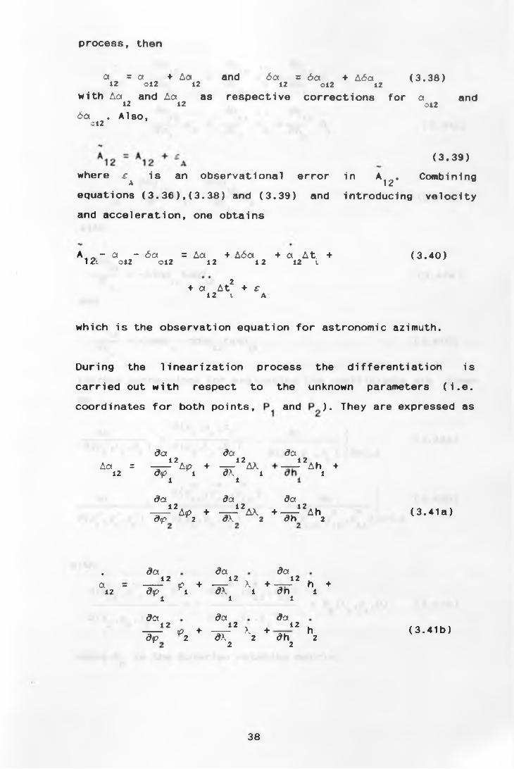
which is the observation equation for astronomic azimuth.
During the linearization process the differentiation is
carried out with respect to the unknown parameters (i.e.
coordinates for both points, and ). They are expressed as
6a = 12
da12 .— — A p +
d(p l l
da— 12 AX dX il
da
da da da
12Ah +l
1 2 . t2 1 2 ,,— — A <p + -rr— AX + -z— Ah d<p 2 dX 2 dh 2
(3.41a)
. da da da12 . 12^ 12 a - — — <p + -3r* X + h +
12 dp i d\ i dn i i i l
da12--- P +
d<p 2
da da12 x 12 . -rr— X + hdX 2 dh 2
2 2
(3.41b)
38

a12
da
d'f
da
dp
12 • •
” , +
d a12 • •
>d a
12-A.1 d \
11 dh
i
12 • m?2 *
d a12 • •
xda
12-i.2 2 dh
2
h1
h2
+
d6a ddaA6a = -=-12A{ + — 12Ar)
d£ i dr\ i i 'i
12
with
d6ct12
__ = -sina tary?91 12 ' 12
and
dda12 = -tarv - cose- tan,? dr; ^i 12 ’ 12
Further expressions for evaluating the coefficients
as
da * ( V W dad(f, A ,h ) a(*>A ,h ) *
k k k k k k d ( x , , y , z t )k k k
k=i ,2
da
* K * v zJ>k k k
♦ ♦ ♦d(x ,y ,z )
12 12 12 da* * ♦
d(x , y ,z ) 1 2 12 12
k=l ,2
with
= R (\ ,0 ,0)E l l
where R is the Eulerian rotation matrix.E
♦ * *d(x ,y ,z )
12 12 12
d (x, . y,.z, )2 2 2
♦ * *d(x , y ,z )
12 12 12
a(Xl ,yi »Zi )
(3.41d)
(3.41e )
(3.41f )
are given
(3.42a)
(3.42b)
(3.42c)
(3.41c)
39

3.3.6 Vertical angle
From a point to another point P^, the vertical angle B 1 2 12
between the two points is represented as
B12
tan - 1 12♦ 2 *2 1 / 2(X + Y )12 12 - *
(3.43)
The vertical angle may be further decomposed into a model
component (1 and a disturbing part 6(1 such that12 12
B = 0 +6/?12 12 12
(3.44)
with
(1 - tan12
-1 12
L, ♦2 *2 1/2(x , + y )
12 12
(3.45)
Suppose that B is the observed value free from refraction12
and B is the actual observed value containing effects of12
refraction 6r, then
B = B + 6r (3.46)12 12
with
B = B + £12 12 B
thus- n +6/? + £' 12 12 B
B = (1 + An + 6(1 + A 6(1 + 6r + A 6r + £12 012 12 012 12 O B(3 . 47)
on taking the approximate values, for (1 , 6 ? and 6r as
(1 . 6(1 and 6r respectively, for use after a Taylor' 012 012 o 0series linearization. On considering the observed angle B
12
and incorporating the velocity and acceleration unknowns,we
have
40

( 3 . 4 8 )
4= A/? ♦ A6fi + A6r +
12 12
♦ p At + (1 At2 ♦ £12 i 12 i B
and A/?i2 , A6/?^ and A6 r as respective corrections to be added
to the initial values p , 6(3 , and 6 r . £ is an012 012 o bobservational error in B .
12
Equation (3.48) represents the basic form of the observation
equation for vertical angle. The corrections are expressed as
differential equations in the unknown parameters (i.e. station
coordinates for both points and and also the components
of the deflection of the vertical at the observing point.
a sn12
ddp ddp12 a ? + 12 An1 — --- 1 (3.49)
l lhaving treated the rotation elements as zero. The coefficients are
ddp1 2 ddp= -coso. and
12
12 = si no dT) 12
(3.50a)
Also
dp dp dpAp * - ^ ax * -^r^"Ah +12 dip i d\ i dh i
dp dp dp12 + 12 + 12+ -r----A <p — --- AX -rr--- Ahd<P 2 d \ 2 dh 2
r 2 2 2
(3.50b)
41

dpP --~---- Pi2 dp i
ap .‘2> ♦
dp . 1 2 h
dX i 1 dh i i
dp . ^ dp . ^ dp12 + 12 ♦ 12
dp ^2 dX 2 dh 2 2 2 2
d/? . . dp . . dp . .12 + 12x + ' 12lp — -— X — ---h +12 dp ■ i i dX i dh il l
dp . . dp . . d/?12 + 12 + 12+ -----p ----- X. ----- hdp f 2 dX 2 dh 2
with
dp12 a(V W 1 2
* (W V * (W V ^ V W k=i ,2
and
dp12
♦ * *d( x ,y ,z )
12 12 12dp1 2
a ( x k ’ yk ' z k ) ^ v w* •
d( x ,y ,z )12 12 12 k
3.3.7 Spatial distance
The spatial distance between two points and P^
expressed mathematically in the form
12 ■ f*2 *2 *2X + Y + Z12 12 12
with the model part s expressed in the form12
1 2 = i ♦2 *2 *2x + y + z12 12 12
Since distances are not influenced by effects of the
(3.50c)
(3.50d)
(3.51)
1,2
(3.52)
may be
(3.53)
(3.54)
gravity
42

field, the disturbing component becomes equal to zero so that
S = s 12 12 (3.55)
Further, let s be the approximate value for 8 , then012 12
s = 8 ♦ As12 012 12 (3.56)
where As is a correction to be added to the initial value12
s . Also suppose a value for spatl a 1 distance isQl2 121observed at epoch i, with a random error in it, then
S.. . = s + £ 1 2 i 12 s
(3.57)
Combining equations (3.56) and (3.57) and including velocity and acceleration one gets,
• • •S . - s = As + sAt + s At2 + £ (3.58)12l *12 12 i i s
which becomes the observation equation for distance. The
parameters are expressed in the following differential
equations,
ds ds ds12. 12. x i 2 t. +As = — ----Ap + -~r----AX + -z—---Ah12 dp l ok l un l
ds ds ds12. 12 . 12+ — ----Ap + — ----AX + ----- Ahdp r 2 dX 2 dh 2 (3.59a)
ds . ds . ds12 + 12 -I- 12Si2 dp ^i dX i dh i
i i i
ds . ds . . ds12 + 12 + 12+ ----- p ------x ——----ndp f 2 dX 2 dh 2 * 2 2 2
(3.59c)
ds .. ds .. ds12 + 1 2 + 12
S = ------------P rr-------- X —rr-------- 1! +12 dp Vi dX 1 dh 11 1 1 3
3S12 " + aS12 " +* dip ^2 9\ 2 dh 2r 2 2 2
(3.59d)
43

and also
ds12
* (W V
and
* ( V W
* (W V
ds12
* ( v w k=i ,2(3.60a)
ds12
* ( V W
d U l2 ' \ t ' \ z )
* ( V W
ds1 2♦ ♦ ♦
d( x , y ,z ) 12 12 12 k =i ,2
(3.60b)
3.3.8 Horizontal direction
Let the horizontal direction of an observation line be
T at observation point P . Further let the azimuth of this 12 1line be A^: then,
T12 = A12 (3.61)
ter at the standpoint Pwhere is an orientation par
Decomposing the azimuth of tnis line into a model part a
a disturbing part do cne obtains12
1and
1" = a + 6a + r12 12 12 “I(3.62)
with a defined in equation (3.36). Taking initial values for 12
a and 6a we form equation (3.38) and incorporating r into12 12 ^equation (3.39) we arrive at the modified azimuth equation
T - a - 6 a = La + _lra + a At + a At + T1 2 i * 12 912 12 12 12 i 12 t U1
♦ £ (3.63)
where £ is an observational error in the directionT
44

observation T12i
Equation (3.63) is the observation equation for an observed
horizontal direction.
Expression for Aa and Ada are given in equations (3.41).12 12
The final coefficients are as provided in equations (3.42).
3.3.9 Gravity potential difference
The difference in gravity potential between two points
and is of the form2
W = W - W (3.64)12 2 1
On considering the model and the disturbing components (see
also section 3.3.1), we get
W = w - Aw12 12 12
wherew = w -w and 6w - 6 w - 6w
12 2 1 12 2 1The observation equation is of the form
W1 2 iw - 6w = Aw + A£w + w At +c 12 012 12 12 12 i
. . , 2+ W At + £12 l v12
(3.65)
(3.66)
(3 . 67)
The parameters are expressed as
dw dw dwAw = 12 A<p + i2~ AX + — -— Ah +
12 dp 1 ok 1 dh1 i i
dw dw dw12 . . 12 .. 12+ ---- A<p + --- AX + — — — Ahd > ^2 dX 2 dh 2(3.68a)
and A6w = A6w - A6w 12 2 1
(3.68b)
45

dw . , dw dw .• 12 + ___ 12 ♦ 1212 dp i dk t dh ii i i
dw . m dw d w .12 ♦ 12 x ♦ 12 .♦ --------------- --------------------------------- X ----------------h
dp v 2 dk 2 d h 2 2 2 2
d w . . . d w dw. . 12 ♦ 12 + 12.w = — --- p — —— A. ——-— h +12 dp i dk i dh i i i i
dw .. d w .. d w+ ---------------<D -----------------X ---------------- h
dp f2 dk 2 dh 22 2 2
3.3.10 Gravity difference
The difference in gravity r between two points, P12 1
(see also section 3.3.2) is
r = r - r12 2 1
On separating the model portion y and the disturbing
one may write
f = y + by 12 12 12
wherey = y - y and by - by - by 112 { 2 fl 12 2 1
The observation equation is therefore of the form
r — y — by - A y + A by + y At +12l * c!2 ' C l2 * 12 12 #12 l
+ y At. ♦ £„i 2 v r (3
The expressions for the parameters are
(3.68d)
and P,.2
(3.69)
part by,
(3.70)
(3.71 )
.72)
(3.68c)
46
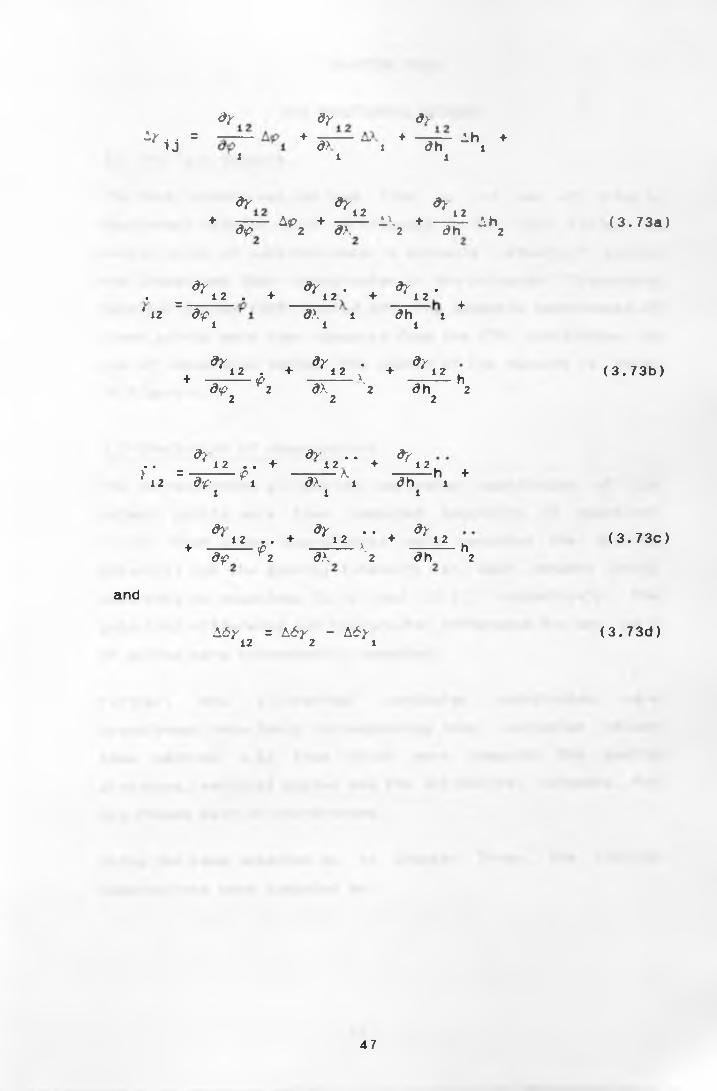
dy dy d>
Ly i j = + d > ~ ~ 1 * “ d h ~ l h ! *i 1 l
dy dy dy♦ —— A p ♦ —1* a\ ♦ _ Li ih
dp p 2 d\ 2 d h 2 (3.73a)
. _ * i2 . + ^12* ♦ ^12** 1 2 ” dp d \ i d h i *1 1 1
dy dy . dy' 12 . + 12 A ♦ 12 ,+ ----- 0 ----- X ------hdp f 2 dX 2 dh 2
2 2 2
(3.73b)
d d> . . dy. . 1 2 . . + 1 2 + * 1 2> r --------------- 0 ---------------A. ------------- h +' 1 2 dp f i dX 1 d h 1
i l i
dy dy .. dy*12 . . + 12 + *12+ ----- 0 ----- X ------hdp y2 dX 2 d h 2
(3.73c)
and
A6y = A6y - A6y12 2 1
(3.73d)
47

CHAPTER FOUR
THE MONITORING NETWORK
4.1 The Test Network.
The test network was derived from an old map of Olkaria
Geothermal station which is situated in the Rift Valley in
Kenya, South of Lake Naivasha. A suitable network of points
was chosen and their coordinates in the Universal Transverse
Mercator System (UTM) scaled off. The geodetic coordinates of
these points were then computed from the UTM coordinates by
use of conversion tables. The sketch of the network is shown
in Figure 4.1.
4.2 Simulation of observations.
The corresponding ellipsoidal cartesian coordinates of the
network points were then computed according to equations
(3.10). From these coordinates were computed the gravity-
potential and the gravity intensity at each network point
according to equations (3.15) and (3.21) respectively. The
potential difference and the gravity difference for any pair
of points were subsequently computed.
Further, the ellipsoidal cartesian coordinates were
transformed into their corresponding local cartesian values
(see section 3.2) from which were computed the spatial
distances, vertical angles and the ellipsoidal azimuths for
any chosen pair of coordinates.
Using the same notation as in Chapter Three, the various
observations were computed as:

NA
2
Fig 4.1 The sketch of the network
49

(i) Spatial distances S12
♦ 2 * 2 * 2s = ( x + y + z )
12 12 12 12
i/2
(ii) Vertical angles/?12
(4.1 )
si ry? 12
1 212
(4.2)
(iii) The ellipsoidal azimuth, a12
tancx 1 21 2
♦ * *with x = x - x
12 2 1
12
0 0 0y = y - y12 2 1
(4.3)
z = z - z 12 2 1
The elements of the deflection of the vertical were obtained
as explained in section 4.5. These parameters were then used
to convert the geodetic quantities of latitude <p, longitude
X, and azimuth a, into their correspond!'ng astronomic
quantities, $, A, A, according to the following equations
e.g Heiskanen & Moritz, 1967,pp.187]
$ = <p + £
A = X + T)sec<p
A = a + r)tan<p
(4.4a)
(4.4b)
(4.4c)
The computed observations were perturbed each according to
the assigned standard error. Thus,
y = }JL ± or.. z (4.5)
where y is the perturbed observation, /j the true
observation, o the associated standard error of that
observation and z is a random number. The random numbers were
generated by a function in the Mainframe Computer (VAX 6310)
50

and the actual perturbations computed according to (4.5)
using a computer program listed in appendix Cl. The weights
were computed as explained in the next section.
4.3 Weighting of observations.
Weights are related to the variance in the following
?crow. - ----1 t
where cr is the variance of unit weight, also called o2factor or sometimes the variance component,
variance of observation i. Using the matrix notation
represent the weight matrix, W as
way
(4.6)
vari ance
i s the
we may
w - a T ' (4 . 7 )o “ y y
where T is the variance covariance matrix of the
observations. Therefore from (4.6) we note that the problem
of weight determination reduces to that of determining the
standard errors for the observations.
In this section are discussed the various ways used for
assigning standard errors to the different observations.
4.3.1 Gravity potential differences.
Gravity potential differences can be obtained from precise
leveling observations where gravity values are also measured
(Heiskanen & Moritz, p.160-162). The accuracy of precise
leveling is quite high. The standard error per kilometre can
reach r0.3 to 1.0mm [Mueller et al, 1979].
The United States standard for national vertical control for
first order work is 3mm|k for class I, where K is the total
leveled distance in kilometres [Mueller et al 1979]. For this
first order work, the accuracy of the gravity potential
requirement is stated to be ±2x10 m s . From simple
51

calculation on error propagation and assuming K is not large,
the accuracy of the geopotential number obtained is of the
order 10 m s"
In this study the a priori standard error for the potential
difference was adopted to be 5x10 m s .
4.2.2 Gravity differences.
The standard errors of the International Gravity
Standardisation Net 1971 (IGSN71) is quoted to be less than-2
10.1x10 ms for some values [Torge,1930] while the global-*5 -2
relative standard error of the network scale is *2x10 ms .
In case of gravity difference measurement with gravimeters, a-*5 -2
standard error of approximately ~0.01 to dO.05x10 ms can
be obtained [Torge,1930] . This can further be improved to— H — 215x10 ms by using LaCoste Romberg gravimeters [MaConnell
et al, 1975]. With this wide choice of accuracy, it seems
that one would still be within limits if he uses a value of
*1x10 ms ' which is used in the present study.
4.3.3 Astronomic latitudes.
The standard error for astronomic latitude is estimated to be
0".33 [e.g Robbins, 1976]. Other values quoted are 0M.25,
and .0".2. A value of rOM.3 was used throughout the
computations as the standard error for astronomic latitude.
4.3.4 Astronomic longitudes^
Aduol (1981) used the a priori standard error of astronomic
longitude as ±0.5seoi>. This value had been estimated by
Robbins (1976). In Torge (1980) an accuracy of about ±0".5 -
1".0 is attainable for longitude observations. For the
present study the value adopted is 10".5 since the variation
of longitudes in the network considered is very small - less
than 1”.
52

4.3.5 Astronomic azimuths
Bomford (1980) estimates the standard error for azimuth as
T ’.O. Aduol (1981) used a value of -O'*.7 which he had found
consistent with values from various sources [Davies et al,
1971], Ordnance Survey, Stolz (1972), and others. The value
of 0".7 is adopted for this study.
4.3.6 Vertical angles
The vertical angle can be observed with a standard error of
the random component of about rOM.4 to iO.M6 [Hradilek,1984].
However this value may deteriorate to about z1M.2 to 3" owing
to systematic effects.The overall standard error of a
vertical angle can be expressed as
S; = s' + s' (4.8)•>/ o r
where S is the standard error of observed vertical angle, S
and S are the effects due to the random and refractional
effects. Aduol (1931) used a value of -0.001 for standard
error of the refraction component which he had found from the
results of Hradilek (1973) and Ramsayer (1969). Since the
present study is conducted using purely simulated data, it is
free from refractional influences and it was found convenient
to use a common value of t 1" for standard error of the
vertical angle.
4.3.7 Spatial distances.
The most precise distances are measured with electronic
distance measuring instruments (EDMs), such as a Mekometer ME
3000. The standard error of these instruments consists of two
parts, a constant part and the observational part. The
observational part is dependent on the length of the measured
line whereas the constant part is the same for a particular
instrument. Rueger (1983) had estimated the Mekometer
53
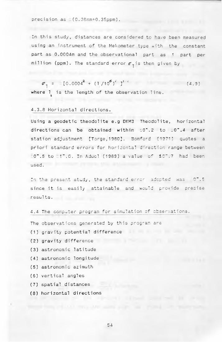
precision as (C. 38/r.m+0.35ppm).
In this study, distances are considered to have teen measured
using an instrument of the Mekometer type with the constant
part as 0.0004m and the observational part as 1 part per
million (ppm). The standard error <r,is then given by
£T, = [0.0004* + (1 /10®)' ]' 2 (4.3)
where 1 is the length of the observation line.i
4.3.8 Horizontal directions.
Using a geodetic theodolite e.g DKM3 Theodolite, horizontal
directions can be obtained within i0".2 to z0".4 after
station adjustment [Torge,1380]. Bomfcrd (1371) quotes a
priori standard errors for horizontal direction range between
0".5 to 1". C. In Aducl ( 1989) a value of 10”. 7 had been
used.
In the present study, the standard error adopted was CM.5
since it is easily attainable and would provide precise
results.
4.4 The computer program for simulation of observations.
The observations generated by this program are
(1) gravity potential difference
(2) gravity difference
(3) astronomic latitude
(4) astronomic longitude
(5) astronomic azimuth
(6) vertical angles
(7) spatial distances
(8) horizontal directions
54

The program was written on a mainframe computer (VAX 6310) in
FORTRAN language. The program consists of essentially four
parts: the first part involves reading the data from a data
input file, the second part performs the computation of
various observations associated with the observation lines
read in the first part. The third part consists of a
perturbation routine which transforms the computed data into
"field data". The last part consists of various subroutines
that are needed. A flow chart for the program is presented in
appendix B.2 and the program listing in appendix C 1 .
4.5 Elements of the deflection of the vertical
The elements of the deflection of the vertical are commonly
decomposed into two parts: the north-south component, * and
the east-west component, 77. The mathematical models of
Chapter three require that approximate- values of these
elements be known before the adjustment is made.
The deflection of the vertical elements can be determined
from astronomic and geodetic measurements [e.g. Heiskanen &
Moritz, 1967 pp.223] as
£ = $ - <p (4.10a)
77 = (\ - A)cosp (4.10b)or by using the gravity anomalies, Ag as given by the Vening
Meinesz formulae [e.g. Heiskanen & Moritz, 1967 pp.114]
s h r j J A 9s1nv'o o
dS(y)cosctdu'dad(y) (4.11a)
77 277
.[O
The deflection of
equations (4.11)
. . dS( i') .Agsinv' —rr2t S1 d(y)
the vertical
have the same s
nact y ' da
values
i gn as
obtained
those of
(4.11b)
by using
equations
55

equations (4.11) have the same sign as those of equations
(4.10) but differ in that the astrogeodetic deflections are
oriented with respect to the geodetic coordinate system.
Computations of equations (4.11) require values of gravity
anomaly to be known and also the computation is usually
lengthy and difficult.
A computer program in FORTRAN for computation of gravimetric
quantities from high degree spherical harmonic function is
given by Rapp (1982). However this program was not used as
the values obtained are of the type (4.11). For this study,
the elements of the deflection of the vertical were computed
from astronomic coordinates which have been computed from the
gravity potential [e.g Ashkenazi 1983]. The values used are
shown in tables 5.2.
Equations (4.10) are then applied.
4.6 The free network solution
Since distances and azimuth observations were present, the
network needed to be controlled only in the translational
elements namely X, Y, Z or <p, X , h. Therefore the restriction
matrix of equation (2.18) becomes
$ = tan-1 Z (4.12a)
(4.12b)
1 0 0 1 0 0 1 0 0
G = 0 1 0 0 1 0 . . . 0 1 0 (4.13)
0 0 1 0 0 1 0 0 1
56

Z. However, in the present computations the datum was defined
over approximate coordinates in curvilinear form, that is in
P » *■» h * The G matrix was therefore transformed to G to conform with the datum coordinates as
G = GJG’
where J is a 3x3 coefficient matrix defined as
(4.14)
r
j =
L
dx/dp dy /dp dz/d'p
dx/dk dy/dk dz/dk
dx/dh dy/dh dz/dh
1
(4.15)
57

CHAPTER FIVE
THE NETWORK DESIGN AND COMPUTATIONS
5.1 Introduction
The establishment of a geodetic network includes the
following steps in order of execution:
(1) field reconnaissance
(2) design of the network
(3) marking of the points
(4) carrying out the observations
(5) network adjustment
(6) interpretation of the results.
In the second step, of network design, Grafarend (1970) has
identified four orders in the design of a survey network.
These orders are as outlined below:
The first order, called the Zero Order Design (ZOD) is the
search for the optimal datum. The datum is usually determined
by the nature of the problem, for example in absolute
networks, the reference stations provide for the datum. In
the present study the datum is defined through the
approximate coordinates that have been used, within the
framework of a free network.
The First Order Design (FOD) is the next level and refers to
the configuration of the network, where the positioning of
the points and the observation plan are to be optimized.
The Second Order Design (SOD) is the weight problem, that is
the distribution of various accuracies to the different
observations.
5*

The Third Order Design (THOO) refers to the optimal
improvement of an already existing network by addition or
deletion of points and /or observations. This stage is not
considered for the present study.
The need for network design is to minimise "over surveying"
as this is labour and time consuming. As already indicated,
the actual position locations will not be investigated as
these are constrained by other factors beyond this study,
such as area topography, geology and station access.
In the approach to the solution of this problem, one
recognises the three general criteria [e.g Schmitt, 1990] of
precision, reliability and economy. The ideal situation is to
express the three criteria as an analytic function which one
then optimises. However, owing to the difficulties involved
in establishing this general function, particularly in three
dimensional networks, the present study adopts a different
but satisfactory method.
In this study, the weights that are assigned to the
observation values are considered optimal as these are based
on wide experiences from various reports on different
surveys. However, the main interest in this study is to find
the optimal number of observations for each observation type.
The procedure adopted for optimization is by computer
simulation method through the variance component estimation
as explained in section 5.2.1. This procedure has an
advantage in that it permits the possibility of using
arbitrary decision criteria for the choice of an optimal
design without having to formulate the objective functions in
analytic forms.
59

5.2. Network simulation.
The parameter estimation model of the Gauss-Markov type is
given in Chapter Two as
y = Ax + e with D(y) = D(^) = T (5.1)<-yy
The parameter vector is then given by
x “ (A'WA)~ 1 A ’Wy (5.2)
and the dispersion Y of x is given byx x
r - o* (A’WA)'* (5.3a)X X O
and the dispersion Y of the estimate y of y is given byyv
Y = A7 A ” (5.3b)y y xx
and o' is the variance of unit weight. Y is the covarianceo * X
matrix of parameters.
For a survey network, x is the vector of the coordinates or
their small corrections, y the vector of observations and A
consists of the values computed from the mathematical models
using the approximate station locations. The precision of the
network is then assessed by analysing £
The criterion for assessment used in this study is the size
of the absolute error ellipsoids. The values obtained are
shown in the tables in section 5.4
Further to the analysis of the variance-covariance matrix £xy
, a posterior variance of unit weight o is also computed
from [e.g. Mikhail, 1976]
o ” (n+r-u)where n is the number of observations, r is the number of
restrictions and u is the number of parameters. The a priori
value of o is taken as unit.o
60

5.2.1 The variance component estimation
Consider the Gauss Markov model [Aduol, 1989]
y = Ax + c (5.5)
with E(r) = 0, D(r) = . = D(y) = £
In order to solve a survey network, one normally observes
different types of observations such as distances, angles,
directions, vertical angles, azimuths etc. In this case then,
one may consider the vector y of (5.5) to consist of several
subvectors y , with each subvector containing a differentiobservation type. Associated with each subvector y » is a
variance component for that observation type a . EquationOr.
(5.5) would then be represented as
(5.6)r y.l
1<1__ £1
y2: ! *
A2l
x + £2----
11 •
>*____
1IA,Jr
mm — n• V)____
1
witn ** ^(0,r ) = (0%o~ w ),
types.
1(1 )k, for k observational
The dispersion of y, D(y) is obtained as
D(y) =D( ) =
J
w 1C l 11
O' W o 2 22
» r Jok kk
(5.7)

On taking u = w , (5.7) becomes
D(y) =
— •>. Q • v i 1 1
i2 QC 2 2 2
(5.8)
2 _, Q ,c k k k —
Q is the cofactor matrix of the observations while £ is
the covariance matrix of the observational type y . Fromi(5.6) and (5.8) it can then be shown that
Q
Q Q . . . Q£ 1 £ 1 £l£2 £ i r k
Q Q . . • Q£2£t £2£2 £ 2 £ km
Q Q . . . Q£ k £ i £ k £ 2 £ k £ k
(5.9)
for which one writes
Q = Q - AQ A' (5.10a)Cm \ f •. / W Wor equivalently,
Q = w'1- A(A’WA)"'a ’ (5.10b)
The various variance components may now be estimated as in
Aduol (1983)
T !
2f ICl i
* 2 • ft I" c2 |
£ ’W £i ii i 1
£*W £2 22 2
£ ’W £k kk k
(5.11)
• > 62

Lne parameters. Therefore the numoer of measurements for eacn
observation type can be altered oepending on its
contr1Dution.
Before tne number of observations are altered, it is
necessary to set some accuracy criteria that the system must
achieve. In the next section some precision criteria are
reviewed and a choice as to which criterion to use is made.
Of importance is the question of which particular observation
should one drop out during the optimization. A possible
solution is to ensure that the remaining observations are
uniformly distributed as much as is possible.
In this study, the remaining observations were kept uniformly
distributed as much as was possible. The observations whose
residuals appeared greater, though within acceptable limits,
were also eliminated.
With regard to the astronomic observations, namely latitude,
longitude and azimuth, special attention was given. The
requirement was that these quantities be observed from the
same stations as much as possible since this could minimise
travelling expenses and again it is sometimes possible to
observe these quantities simultaneously.
5.3 The precision criteria.
The quality of the adjusted coordinates of the network are
analysed via the network’s a posterior variance-covariance
matrix according to equation (2.3)
(5.15)
where <y2 is the variance of unit weight.o
64

5.3.1 Positional standard errors.
The positional standard errors of the parameters (i.e
coordinates) are obtained by simply taking the square roots
of the diagonal elements of the variance-covariance matrix,
D(x). The size of the standard errors are dependent on the
chosen datum [e.g Cross, 1979]. For this reason, the
positional standard errors are not quite useful as tools of
network analysis. However, in this study, they have been
computed since the network was adjusted on the basis of a
free network where no coordinates had been fixed (see section
2.1.3).
5.3.2 Spherical standard error and spherical probable error.
Spherical standard error, a is a single measure for threeAdimensional cases and is given by [Mikhail, 1976]
Cf --T- {a + a + O' ) (5.16a)s 3 x y z
where c? , <y , and a are the standard errors in X, Y, andx y =
2 respectively.
Closely associated with a is the spherical probable error
SPE defined as [Mikhail, 1976]
SPE = 0.513(0' + c + Cf ) (5.16b)for 0.35< (c- /a )<1.05 yy.
5.3.3 Mean radial spherical error (MRSE)
This is defined as [Mikhail, 1976]
MRSE (5.17)y
65

5.3.4 Standard error ellipsoids.
Using matrix and vector notation and simplifying, the function
X ’£ ”‘x = 1 (5.18)
where X is the vector of parameters and £ is the covariance
matrix. Equation (5.18) represents the equation of the
standard error ellipsoid. The semi axes of this error
ellipsoid are the square roots of the eigenvalues of the
variance-covariance matrix and their directions are computed
from the eigenvectors of those eigenvalues [Hirvonen, 1971].
The probability of a point falling on this standard ellipsoid
is 19.9% [Mikhail, 1976]. The advantage of using the error
ellipsoid as a tool for network analysis is that the values
obtained for the computation of the ellipsoid are derived
from the whole set of the variances and covariances unlike in
single measure criteria where only the diagonal elements are
consi dered.
5.3.5 Concluding remarks.
From the foregoing, one notes that the single precision
criteria uses only part of the information concerning the
precision of the network and as such is therefore not a very
good precision criteria to use. On the other hand, the error
ellipsoids make full use of all information concerning the
precision of a network.
Therefore for this study the values of the error ellipsoids
are computed and as a single precision criteria the spherical
standard error o is also computed. And since the9
mathematical models being tested are required for precise
monitoring networks we set as a general requirement that each
66

of the axes of the error ellipsoids do not exceed 10mm.
5.4 The Results of computations for initial epoch.
5.4.1 Test I
Test I was the fully observed model and was considered to
contain the highest number of observations (not necessarily
all possible observations). The present network consisted of
26 possible observation lines for double observations and 6
possible observations for point observations. All possible
observations could be used during the computations but since
it is not always possible (owing to field conditions) to
observe all possible lines the following choice was made: all
six point observations and 24 double line observations were
assumed to have been possible to observe.
The full model was considered to yield results of highest
accuracy. The observations used for this model are shown in
Tables 5.1 and the approximate coordinates together with the
elements of the deflections of the vertical are shown in
Tables 5.2. The results of the computations for this model
are given in Tables 5.3, 5.4 and 5.5.
In Table 5.3, the trace refers to the redundant observations
as computed according to equation (5.13). The "observations
used”, here refers to the actual number of observations that
were used in contributing towards the estimation of the
unknown parameters. The rest of the other observations were
only necessary for improving the adjusted observations and
are here referred to as “observations left".
67

Table 5.1 The simulated observations of the full model
(a)
STATION ASTRONOMICLATITUDE
ASTRONOMICLONGITUDE
1 -0e
51 38 .330 360
19 18 .0232 -0 51 13 .523 36 17 59 .5703 -0 52 08 .561 36 19 34 .5314 -0 52 05 .417 36 17 58 .4535 -0 53 10 .269 36 19 32 .2736 -0 53 03 .861 36 18 15 .211
(b)
LINE DISTANCE (metres)
HORIZONTALDIRECTION
VERTICALANGLE
1 2 2550.29320
287 33 36.384
-3 -48 -39.681 3 1106.5828 151 20 30.06 -15 -41 -10.901 4 2609.1804 251 11 46.19 -4 -53 -52.321 5 2893.3510 171 1 1 1 .25 -5 -59 -3.522 1 2550.2929 107 33 37.91 a 47 17.432 3 3397.3061 120 6 5.88 "2 -12 -35.872 4 1606.9482 181 14 37.00 -54 -21.312 6 3448.4205 171 56 22.06 -1 -16 -48.613 1 1106.5826 331 20 29.88 15 40 36.663 2 3397.3041 300 6 4.25 2 10 46.103 4 2974.3997 271 52 4.44 1 28 2.673 5 1910.0090 182 5 50.06 0 -3 -56.024 1 2609.1800 71 1 1 47.25 4 52 28.374 2 1606.9473 1 14 37.23 1 53 29.14
1 4 3 2974.3996 91 52 5.81 -1 -29 -38.394 5 3528.4614 124 39 1 .75 -1 -17 -41.764 6 1880.7889 164 0 12.06 0 -42 -17.705 1 2893.3513 351 1 1 1 .38 5 57 30.305 3 1910.0093 2 5 49.92 0 2 53.915 4 3528.4620 304 39 0.25 1 15 47.575 6 2392.4915 274 44 40.69 1 19 41.276 3 2991.6447 55 6 41.52 -1 -2 -52.006 4 1880.7901 344 0 12.25 0 41 16.29
6______
5 2392.4917 94 44 42.13 -1 -20 -58.32
68
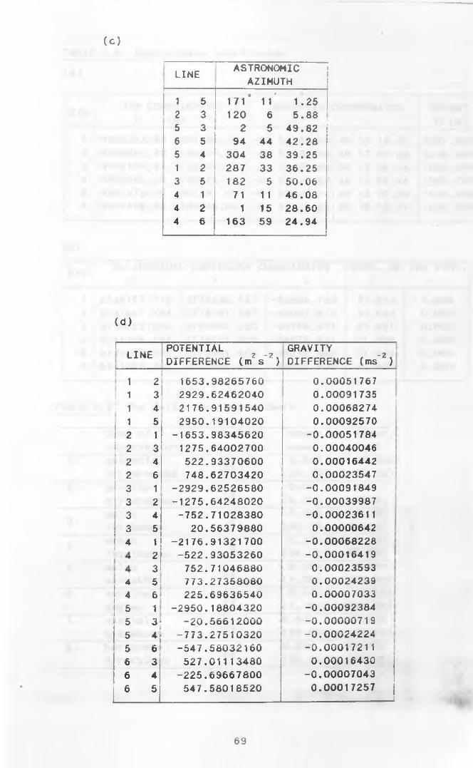
( C )
LINE ASTRONOMICAZIMUTH
1 5 171O s
1 1 1.252 3 120 6 5.885 3 2 5 49.826 5 94 44 42.285 4 304 38 39.251 2 287 33 36.253 5 182 5 50.064 1 71 1 1 46.084 2 1 15 28.604 6 163 59 24.94
(d)I-------LINE
;________POTENTIAL DIFFERENCE ( m V ?)
GRAVITYDIFFERENCE (ms"2)
1 2 1653.98265760 0.000517671 3 2929.62462040 0.00091735
I 1 4 2176.91591540 0.000682741 5 2950.19104020 0.000925702 1 -1653.98345620 -0.00051784
i 2 3 1275.64002700 0.000400462 4 522.93370600 0.000164422 6 748.62703420 0.000235473 1 -2929.62526580 -0.000918493 2 -1275.64248020 -0.000399873 4 -752.71028380 -0.000236113 5 20.56379880 0.000006424 1 -2176.91321700 -0.00068228
2 -522.93053260 -0.000164193 752.71046880 0.00023593
4 5 773.27358080 0.00024239
I 4 6 225.69636540 0.00007033
I 6 i -2950.18804320 -0.000923845 3' -20.56612000 -0.000007195 4; -773.27510320 -0.000242245 6 -547.58032160 -0.000172116 3 527.01113480 0.000164306 4 -225.69667800 -0.00007043
!_!_5 547.58018520 0.00017257
69

Table 5.2 Approximate coordinates
(a)
UTM COORDINATES X (m) Y
GEODETIC COORDINATESX
HEIGHT h (m)
1 ;9904334.88 201888.29 -0J 51 59.55 36 19 18.02h2207.900
2 *9904890.75 199460.91 -0 51 34.56 36 17 59.58 2038.9003 9903189.63 202400.07 -0 52 29.98 36 19 34.54 1908.8004 9903284.36 199426.75 -0 52 26.83 36 17 58.44 1985.7005 |9901279.96 202331.63 -0 53 32.11 36 19 32.28 1906.9006 ;9901476.98
i_____!____________199946.84 -0 53 25.67 36 18 15.21 1962.800
(b).STNi
ELLIPSOIDAL CARTESIAN COORDINATESX Y Z
DEFL. OFe
THE VERT.r)
i 5140177.718 3778830.147 -95838.194 21.213 0.0002 5141487.484 3776781.987 -95067.973 21.044 0.0003 5139622.594 3779056.330 -96768.421 21.421 0.0004 5141446.194 3776707.306 -96672.831 21.400 0.0005 5139638.794 3778981.400 -98676.885 21.844 0.00061 5141097.793 3777095.873
_____________-98479.939 21.800 0.000
__________ 1
TABLE 5.3 The fully observed network.
type of observation
total no. of obser.
obser.used
obser.left
1 . potentialdifferences 24 4.962
(20.7*)19.038
(79.3*)2. gravi ty
differences 24 0.0(0.0*)
24(100*)
3. astrolatitudes 6 5.803
(96.7*)0.197(3.3*)
4. astrolongitudes 6 5.775
(96.3*)0.225(3.7*)
5. astroazimuths 10 0.099
(1.0*)9.901(99.0*)
6. verticalangles
24 0.417(1.7%)
23.583(98.3*)
7. spatialdistances 24 6.447
(26.9X)17.553(73.1*)
8. hori zontal di rections 24 9.496
(39.6X)14.504(60.4*)
70

Table 5.4 The estimated coordinates for the full model
STATION LATITUDE i p ) LONGTUDE (K) HEIGHT (m) h
10
- 0 51 59.550 36 19 18.020 2207.9012 - 0 51 34.561 36 17 59.581 2038.8993 - 0 52 29.982 36 19 34.541 1908.7994 - 0 52 26.821 36 17 58.440 1985.7015 - 0 53 32.110 36 19 32.281 1906.9006 i - 0 53 25.676 36 18 15.211
__________1962.799 1------------ J
Table 5.5 The parameters of the error ellipsoids for the full
model
station az imuth (cieg; v ..ang1e (Qeg)Sr? (m)
0.0090 235.6 1 .61 0.0020 173.8 -86.6 0.0065
0.0063 145.6 3.00.0097 201.8 2.1
2 0.0022 164.5 -87.4 0.00690.0067 111.8 1.60.0078 215.8 2. 1
3 0.0019 178.3 -87.3 0.00560.0060 1 25.7 1.60.0079 201.1 2.1
4 0.0018 168.8 -87.5 0.00570.0057 111.0 1.30.0097 199.5 1 .7
5 0.0020 161.5 -87.6 0.00660.0064 109.4 1.30.0098 229.2 1.6
6 0.0023 163.6 -86.0 0.00720.0073 139.1 3.6
5.4.2 Test II
Table 5.3 shows that various observation types contributed
differently towards the estimation of the unknown parameters.
Clearly, gravity difference observations were not required at
all in the adjustment since their contribution was OX. These
71
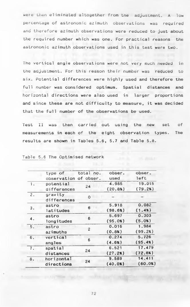
were then eliminated altogether from the adjustment. A low
percentage of astronomic azimuth observations was required
and therefore azimuth observations were reduced to just about
the required number which was one. For practical reasons the
astronomic azimuth observations used in this test were two.
The vertical angle observations were not very much needed in
the adjustment. For this reason their number was reduced to
six. Potential differences were highly used and therefore the
full number was considered optimum. Spatial distances and
horizontal directions were also used in larger proportions
and since these are not difficulty to measure, it was decided
that the full number of the observations be used.
Test II was then carried out using the new set of
measurements in each of the eight observation types. The
results are shown in Tables 5.6, 5.7 and Table 5.8.
Table 5.6 The Optimised network
type of total no. obser. obser.observation of obser. used left
1. potential O A 4.985 19.015differences (20.8%) (79.2%)
2. gravity odi fferencesastro 5.918 0.082
3 • latitudes o (98.6%) (1.4X)astro 5.697 0.303
4. longitudes o (95.0%) (5.0%)5. astro O 0.016 1.984
azimuths c (0.8%) (99.2%)6. vertical CL 0.274 5.726
angles 0 (4.6X) (95.4%)7. spatial O A 6.521 17.479
distances (27.2%) (72.8X)8. horizontal 9.589 14.411
directions 24 (40.0%) (60.0%)
72

Table 5.7 The estimated coordinates of the optimised network
STATION' " —
LATITUDE LONGTUDE HEIGHT (m)
10
- 0 51 59.5500
36 19 18.020 2207.9002 - 0 51 34.561 36 17 59.580 2038.9003 - 0 52 29.982 36 19 34.540 1908.8004 - 0 52 26.821 36 17 58.440 1985.7005 - 0 53 32.110 36 19 32.281 1906.900
6- 0 53 25.676 36 18 15.211 1962.800
Table 5.8 Parameters of the error ellipsoids for the
optimised network
station 1 S T v -(§88)e o , . s (m)0.0057 245.4 1.6
1 0.0013 189.6 -87.2 0.00450.0051 155.3 2.30.0066 184.1 2.2
2 0.0014 182.6 i oo -j 00 0.00480.0049 94.0 0.10.0052 348.7 -2.1
3 0.0012 199.2 i 00 -1 cn 0.00410.0045 78.8 -1.20.0055 351.1 -2.0
4 0.0012 193.3 00r-001 0.00400.0041 81.1 -0.80.0066 183.1 1.8
5 0.0014 180.9
CVJ•00001 0.0047
0.0046 93.1 0.10.0063 225.9 2.0
6 0.0016 174.7 -86.9 0.00500.0057 135.8 2.4
5.5 Epoch II results.
In this second epoch of observations, point 4 of the network
was deliberately displaced by 0”.001 (about 30mm) in
latitude, 0".001 in longitude and 15mm in height. Thus point
4 was taken to be the only unstable point of the object
network. The task was now to estimate the new point position
together with the point velocity including the auxiliary
73

parameters. At first the network was computed as free network
and it was noticed that the displacements that had been
injected into point 4 could not be recovered.
The network was then computed as a fixed one with all other
points fixed except point 4. The results of these
computations are shown in Table 5.9,
Table 5.9 Results of Epoch II observations
1ati tude longi tude—
hei ghtold coordinates -O' 52*26".820 36' 17*58".450 1985.700 mnew coordinates -0 52 26.820 36 17 58.450 1985.700std. error for new coordinates 0".000712 0".000839 0.0075m
point velocity -0.00032 "/yr (^10mm)
0.00179 "/yr 55mm)
-0.0150 m/yr
std. error for point velocity 0.00100 "/yr 0.001188 "/yr 0.0106 m/yr
5.6 Epoch III Results
This is the third epoch of observations. Here, again point 4
of the network was purposely shifted by a further 0".001 of
arc in both latitude and longitude and by 15mm in height. A
different set of observations was computed and these
observations were then used in the kinematic model to
estimate the coordinates of point 4, the velocity of movement
and also the acceleration.
The network was computed as a fixed one with all other points
fixed except station 4. The results of this computation are
shown in Table 5.10
74

Table 5.10 Results of Epoch III observations
latitude longitude » heightold coordinates -O' 52*26“.820 36' 17*58".450
I1985.700 m
new coordinates -0 52 26.820 36 17 58.450 1985.700std. error for new coordinates 0“.00593
. - . -
0".00700 0.06290 m
point velocity -0.00037 “/yr (^11mm)
0.00175 "/yr 54mm)
-0.0149 m/yr
std. error for point velocity 0.0084 “/yr 0.0099 “/yr
"" 1 1 " j 0.0890 m/yr
pointacceleration -0.00055 "/yr 0.00040 ~/yr -0.0068m/yr?
std. error for accelerati on 0.00854 "/yr 0.01012 “/yr2 0.08900m/yr'j
5.7 Epoch IV Results
This epoch consisted of the fourth set of observations.
Station 4 was again allowed to move by a further amount of
0**.001 in longitude only. The new set of observations was
simulated and used in the kinematic model to estimate point 4
position, velocity and acceleration.
The computation of the network is carried out on the basis of
a fixed network. The results of this computation are shown in
Table 5.11
75

Table 5.11 Results of Epoch IV observations
latitude longitude heightold coordinates « ... ! »-0 52*26".820 36 17*58".450 1985.700 m!new coordinates -0 52 26.820 36 17 58.450 1985.700. std. error for jnew coordinates 0".006433 0".00758 0.0687 m
point velocity -0.00051 "/yr 0.00156 "/yr 16mm) (2- 48mm)
-0.0149 m/yr
std. error for point velocity 0.00914 "/yr 0.01078 "/yr 0.0973 m/yr
pointacceleration -0.00006 "/yr2 0.00170 ”/yr
\
2-0.0109 m/yr
std. error for acceleration 0.00809 “/yr? 0.00958 "/yr? 0.08422 m/yr2
5.8 Epoch V Results.
Station 4 was again allowed to shift further by small amounts
of 0".003 in latitude and 10mm in height. The new set of
observations was then computed. The kinematic model was used
to compute the new set of parameters namely point 4 position,
it’s velocity and acceleration together with other auxiliary
data.
Again, the computation of this network was carried out on the
basis of a fixed network. The results of this computation are
shown in Table 5.12
76

Taole 6 . 1 4 Results of Epoch V observations
latitude____ ; longitude neigntold coordinatfcb -0 52*26".820 36 17*58" .450 1985.700 mnew coordinates -0 52 26.820•36 17 58.450 1985.700;sta. error for new coordinates
10" .00063
i0 ”.00082 0.0076m
point velocity -0.00067 "/yr 0.00134 /y r -0.0148 m/yri i i............... i (^2 1mm) (2s 4 1 mm jstd. error for [point velocity 0.00099 "/yr j
i0.00117 "/yr
10.0106 m/yr
pointacceleration -0.00057 "/yr2 j
10.0034 "
*> i/yr 2 1-0.0181 m/yr
std. error for acceleration■■ —- ----— 4
0.00083 "/yr j ... ...... . ■ *
0.00098 "/yr I____ L
i i0.0086 m/yr
The observations of the fifth epoch of observation were again
computed on the basis of a free network, similar to the
initial epoch observations. This static mode of network
computation was made for purposes of comparison with the
results of the initial epoch. The results obtained are snown
in Tables 5.13, 5.14, 5.15 and 5.16.
Table 5.13 Estimated coordinates for Epoch V (fixed mode)
|STATION* LATITUDE LGNGITODc hEIGm T (m; 11 i
i - 0 51 59.550 36 19 18.020 2207.9012 - 0 51 34.561 36 17 59.581 I 2038.8992 - 0 52 29.982 36 19 34.541 1908.799
- 0 52 26.820 36 17 58.450 l 1985.7005 - 0 53 32.110 36 19 32.281 1906.90061________L
- 0 53 25.676________ l
36 18 15.2111
1962.799____________ i

TABLE 5.14 The fifth epoch free network results
type of total no. obser. obser.observation of obser. used left
1. potential 24 4.991 19.009di fferences (20.8%) (79.2%)
2. gravitydifferences 0 - -
o astro 6 5.964 0.0361ati tudes (99.4%) (0.6%)
A astro 6 5.932 0.0681ongi tudes (98.9%) (1.1%)
5. astro o 0.246 1.754azimuths c. (12.3%) (87.7%)
6 . vertical 10 0.131 9.869angles (1.3%) (98.7%)
7 . spatial 24 8.579 15.421distances (35.8%) (64.2%)
8. hori zontal 24 7.158 16.842di rections (29.8%) (70.2%)
Table 5.15 Estimated coordinates for Epoch V observations
(free network mode)
s t a t i o n! LATITUDE LONGTUDE HEIGHT (m)i1
0- 0 51 59.548
036 19 18.022 2207.907
2 - 0 51 34.558 36 1 7 59.582 2038.9073 - 0 52 29.981 36 19 34.543 1908.8074 - 0 52 26.820 36 1 7 58.459 1985.6675 - 0 53 32.110 36 1 9 32.281 1906.9076
________L_- 0 53 25.674 36 18 15.211 1962.607
________________
78

Table 5.16 The parameters of the error ellipsoids (free
network)
station a?lsf v -(§sel
E
•
<D0.0096 191.9 1 .2
1 0.0017 208.9 00•00001 0.0069. 0.0069 101.9 -0.4
0.0127 245.4 0.42 0.0018 163.2 -86.9 0.0083
0.0065 155.4 3.10.0090 315.3 -0.6
3 0.0015 203.1 •00001 0.00640.0065 45.3 -1 .50.0085 310.3 -0.7
4 0.0015 198.0 -88.1 0.00620.0065 40.3 -1.80.0121 246.4 0.3
5 0.0017 163.8 -87.7 0.00810.0067 156.4 2.30.0123 191.4 1.0
6 0.0019 159.6 i CD CD CD 0.00830.0071 101 .4 0.6
5.9 The Main Computer Program
This section explains the program in broad terms only. The
program listings are however given in appendix C2. A flow
chart of the program was also prepared to aid the reader in
understanding the program and is in appendix B2. Part of the
results produced are listed in appendices C3 and C4.
Although separate programs were written for each epoch, these
can be combined into one program which would consist of
basically two controls: one for free network adjustment and
the other for fixed network computation.
The program was written in FORTRAN 77 and prepared on a VAX
6310 Mainframe computer. The storage capacity for this system
was large enough to accommodate the program requirements.
VST

The program consists of 16 segments; the main segment and 15
subroutines. The main segment controls the operation of all
the other segments and also forms the design matrix, the
weight matrix and the observation vector. These segments are
NETWORK: This is the main segment that controls the operation
of all other segments.
RTDMS: Converts radians into degrees, minutes and seconds.
NORMAL: Forms the normal equation’s matrix from the design
matrix and the weight matrix.
EULA: Forms the Eulerian rotation matrix.
MATINV: Inverts the normal equation matrix.
ELLIPSOID: Computes the parameters of the error ellipsoids
for the network points.
RADIAN: Converts angular measurements from degrees, minutes
and seconds into radians.
AZIMUTH: Computes the azimuth of a line from the coordinate
di fferences.
TRANSP: performs matrix transposition.
ELLOR: Computes the vertical angle for an ellipsoidal radius.
VAR: Computes the variance components for various observation
types.
CART: Computes the geocentric coordinates from curvilinear
coordi nates.
ASSIGN: Assigns the various observation lines to their
corresponding codes.
JACCOB: Computes the elements of the matrix of differentials
i n 4>, X. and h .DELTA: Computes the elements of the vector of differentials
in gravity potential.
TIMES: Premultiplies two matrices.
The time required in the central processing unit for running
the program was within the time limit (30 cpu seconds) set by
80

the Insti tute of Computer Sciencethe administration of
University of Nairobi.
m
81
CHAPTER SIX
DISCUSSIONS
This chapter discusses the various findings from the report,
particularly the experiments and attempts to provide possible
explanations to those findings. It is notified here that
other discussions are also made within the report under the
headings "concluding remarks".
During the optimisation of the network, the gravity
difference observations were not required in the estimation
of the parameters as shown in Table 5.3. Since these
observations are necessary, mainly for estimation of the
heights, it therefore meant that the potential difference
observations contributed much more towards estimation of
heights.
A small proportion of astronomic azimuth observations were
"used" in the network while a relatively large proportion of
astronomic latitude and astronomic longitude were "used" as
seen in Tables 5.3 and 5.6. In fact less than one azimuth
observation was needed. Noting that only one azimuth
observation is sufficient to orient a network, it therefore
meant that the remaining proportion to fulfill this
requirement was contributed by the astronomic latitude and
astronomic longitude.
A small proportion of vertical angle observations was
required contrary to the expectations. Since vertical angles
would mainly contribute towards estimation of heights,
deflection of the vertical elements and refraction, it seems
that the basic parameter, height, got a maximum contribution
from potential difference observations. Refraction
coefficients were not estimated and therefore this reduced
82

the requirement of vertical angles. It is suggested here that
in real situations, a maximum number of vertical angles would
be needed, since real data has other systematic influences
such as refraction.
The optimised network turned out to be more precise than the
fully observed network, to the contrary. This could be due to
the fact that during the optimisation process, those
observations with relatively large residuals were discarded.
The proportion of observations that were required towards the
estimation of the parameters are fairly the same for both the
fully observed and the optimised network as shown in Tables
5.3 and 5.6. From this, one may infer that there could be a
basic contributory requirement from each observation type
that must go towards estimating the parameters.
Throughout the computation of the network from the second
epoch up to the fifth epoch of measurement, the new
coordinates of the unstable point remained significantly
unaltered. This is in line with the mathematical models used
for the network computation since all network coordinates for
any epoch are referred to the initial epoch coordinates.
For the second epoch of observation, one is able to estimate
velocity if displacement of a point has occurred. Since the
mathematical models used estimate velocity, the displacement
is obtained implicitly as the product of velocity and the
time that has elapsed between the two epochs of measurement.
In order to test the mathematical models, some shifts were
introduced as shown in section 5.5. To a fairly good
approximation, the models of adjustment recovered these
shifts. This was the case for both the second and the third
83
epoch of observations.
The fourth epoch results were a little different, the model
of adjustment was able to recover, to a good approximation,
the shifts introduced in both latitude and longitude, but not
height. The shift in height appeared exaggerated.
The fifth epoch results also showed that the model was able
to recover, approximately, the shifts introduced in longitude
and height but not latitude.
It is noted that there is a general trend for the model to
slow down the movement of the point in latitude and
compensate this movement in both longitude and height
components. If a point is arbitrarily displaced in each of
the three axes of a coordinate system, it is possible to
return the point to its original position by translation on
only two of the axes combined with suitable rotations. This
could have happened to the adjustment of the network
particularly during the fourth and the fifth epochs.
It is also noted that the third epoch of observation was able
to estimate the point accelerations. This is possible since
there are two velocities between the first and the third
epoch of observation. In fact it was expected that the
estimation of accelerations would improve as the number of
epochs increased since beyond the third epoch of observation,
redundancy in acceleration increased. This is the case as
shown in Tables 5.9, 5.10, and 5.11.
In order to obtain very precise results for the network, the
a priori standard errors of astronomic longitudes had to be
improved from 0".5 to 0".3. This therefore meant that extra
care has to be taken when making these observations. This
84
includes improved methods of observing longitudes.
At the fifth epoch, the network was again computed on the
basis of a free network, just as the initial epoch. It was
noted that the fifth epoch free network coordinates and the
fixed coordinates differ significantly particularly in
longitude, and in general all free network coordinates
shifted significantly so that one is not able to pinpoint
which point was unstable. All the free network heights except
for the unstable point 4 were dispalced by the same amount,
7mm while point 4 was shifted by about 3mm. This shows that
the effect of displacement on point 4 was distributed over
all the other points by the model of adjustment. This
therefore means that if the network was being computed on the
basis of discrete epochs, the varying coordinates of the
network (due to deformation) would not provide sufficient
information on which points were unstable.
85

CHAPTER SEVEN
CONCLUSION
This chapter summarises the work done and gives
recommendations arising from the findings of the work so far
reported.
7.1 Summary
Reported herein are the mathematical models for computation
of localised three dimensional geodetic monitoring networks.
Also considered is the network design aspect.
The mathematical models described here are based on the
kinematic estimation model of geodetic network adjustment
within the framework of integrated geodetic networks. The
design aspect considered was the weight problem for each of
the various observations used. These observations were
astronomic latitude, astronomic longitude, astronomic
azimuth, vertical angles, spatial distances, horizontal
directions, gravity intensity differences and gravity
potential differences. The main parameters computed by these
models were the network coordinates based on the initial
epoch observations, point velocities of the unstable network
points together with the acceleration values where possible.
Other auxiliary parameters were the deflection of the
vertical elements and refraction coefficients.
A test network consisting of six points was computed based on
the proposed mathematical models. Since the study was carried
out by computer simulation, intentional shifts had to be
introduced into one of the network points so as to cause some
network deformation. Five observation epochs were made at a
uniform interval of one year. The initial (first) epoch
observation yielded network coordinates while the second
86

observation epoch, estimated in addition, point velocities.
Third observation epoch together with the succeeding epochs
each estimated network coordinates, point velocities and
accelerations. Although the velocities varied from epoch to
epoch, the network coordinates remained the same as those
computed with the initial epoch observations. All these
realizations were in support of the theory of the
mathematical models used. The displacements computed from the
product of velocity and time reflected the magnitudes of the
intentional shifts that had been injected into the network to
cause deformation.
In order to determine the number of observations needed for
each type of observation, individual contribution of each
type of observation required in the estimation of the
parameters was computed based on the variance component
estimation. From this estimated contribution, one was then
able to alter the number of observations in each type of
observation as necessary. For the test network, it was noted
that only few (about one) of azimuth observations was needed
in the adjustment of the network. Gravity values were not
required in the adjustment while the other observations were
needed in varying proportions as shown in Chapter Five. The
computation of the initial network was repeated with the
optimum number of observations and the accuracy parameters of
the network did not deteriorate; an indication that the
discarded elements were superfluous and therefore not
requi red.
7.2 Conclusions
In kinematic estimation model using the integrated approach,
it is necessary to observe each of astronomic latitude and
astronomic longitude at all stations of the network.
87

Only few (about 1 %) of astronomic azimuth observations are
necessary in a localised monitoring network when using the
kinematic model of adjustment.
Since the optimised network was of comparable accuracy with
the fully observed network, it is concluded that the variance
component estimation procedure through which the optimisation
was made is valid and therefore acceptable.
The kinematic estimation models using the integrated approach
proposed here are capable of detecting point shifts of small
magnitudes: in this experiment, 0".002 in either latitude or
longitude and about 10mm in height could be detected. The
mathematical models are thus acceptable.
The kinematic estimation models provide means for continuous
but pointwise monitoring of ground deformations since
velocities and accelerations are estimated. This continuous
monitoring can also be extended to prediction of deformation
in areas concerned.
7.2 Recommendations
Although the optimisation results require that only few
vertical angle observations are necessary to compute the
network, it is recommended here that a maximum number of
vertical angle observations should be made in order to
estimate and subsequently eliminate refractional influences
which the test data lacked.
It is recommended that as a further test to the kinematic
estimation models, real data should be used and the
stochasticity of the reference network should be taken into
account.
88

APPENDIX A
THE PARTIAL DERIVATIVES USED IN THE OBSERVATION EQUATIONS
The notation used is similar to that used in the text. N and
M are the ellipsoidal radii of curvature in the normal and in
the meridian respectively and e is the first eccentricity of
the reference ellipsoid.
dxdp
dydp
dzdp
, . s . dx . . . dx .-(M + h)sirvcosA, — = -(N + h)cos^sirv., = cos^coaOk On• • • A • 1
d y dy- (M + h )sirv;>sinX, - -(N + h)cos^cos>v, -rr- - cosfsinXok <7h...A.2
z d z(H + h )cos*>, = 0, = sin/> A. 3ok On
OviOX
GMX dvtOY
GMY dw01
GMZ A.4
dOX OX\ /
GM 3GMX23 5r r
d pw] _ 3GMXY ^ x [ a Y j " r 5
d p w -] _ 3GMXZd x j d Z j "
GM 3GMY29 5r r
d Cdvi') _ 3GMYZ < ? Y | d Z j ” r 5
GM 3GMZ2 3 5r r
A.5
89

da♦
y da*
X da1 J _ 1 j w , i j* ♦2 ♦2 ♦ * 2 * 2 * ♦d x X + y . d y X + y d z«-j l j v j «-j ij «-j
* *dr'? X zU _ i J L j
Q; X♦ 1
, * 2 ( X * 2 + y + ♦2
Z*2) ( X
*2 , 1 / 2 + y )IJ l J i j t J
* *W - • y Z
1 J _ 1 j »■ J♦ , * 2 * 2 ♦2 , , *2 ♦2 1/2< ? y . . ( X + y + Z ) ( x + y )t J * j v J 1 J i j
»-J _
dz
*2 t *2 ,1/2 (X + y . )
»• J L J
r *2 *2 *2,(x + y. . + z. . )1 J 1 J V j
ds.. x __VJ _ _ v j .
s .LJ ^
dxcosot cos/?
Lj ij
♦ds. . y___j-j _ _VJ .
* s .d y . . i ]
w
s i not cos/?lj vj
ds z__M . ij .
S
VJ lJdz
sin/?
A.6
A. 7
A.8
90

APPENDIX B PROGRAM FLOW CHARTS
APPENDIX B.1 The Data Simulation Program (SIMUL)
START
l
READ I N DATA
|____ ___________________
1
! • O U T P U T O FC O M P U T A T I O N OF
I H U L*T R U E
O B S E R V A T I O N SO B S E h V A T I O N S
i1
) ' "*
|a
SUBROUT I NFS
PERTURBING THE TRUE
OBSERVATIONS
<-
F I E L D
OBSERVATIONS
END
91

APPENDIX B.2 The Main Program for Adjustment (ADAN)
START
I
i
, READ1. APPR. STATION COORDINATES AND |
OTHER AUXILLIARY DATA i 2. OBSERVATIONS
a) .POTENTIAL DIFF.b) .GRAVITY DIFF.c) .ASTRO. LATITUDEd) .ASTRO. LONGITUDEe) .ASTRO. AZIMUTHf) .VERTICAL ANGLEg) .SPATIAL DISTANCEh) .HORIZONTAL DIRECTION
CONVERT CURVILINEAR COORD. INTO \ GECCENTPIC
j
FORM THE DESIGN MATRIX, THE VECTOR OF OBSER. AND THE WEIGHT MATRIX
•iiiii.
Y
INI-----
INITIAL EPOCH?
>Y
READ MORE DATA?
I NB
92

A B
PERFORM A FREE NETWORK COMPUTATION
VARIANCE COMPONENTS
•
—
r
ITERATECOMPUTE
WEIGHTS AND PARAMETERS
1f
COMPUT E THE I
PERFORM A FIXED NETWORK COMPUTATION
2ND EPOCH? N
COMPUTE.1. POINT COORDINATES • 2 VEL. OF OBJ. POINTS I 3. OTHER AUXILLIARY DATA
COMPUTE THE ERROP ELLIPSOIDS
COMPUTE1.OBJECT COORD.2.OBJECT PT. VELOCITIES 3.OBJECT PT. ACCEL.4.OTHER AUXILLIARY DATA l
ICOMPUTE THE ERROR
ELLIPSOIDS OF OBJ. PTS
COMPUTE THE ADJUSTED OBSERVATIONS
END
93

o o
APPENDIX C PROGRAM LISTINGS AND THE RESULTS
Appendix C.1 program Listing for the data simulation program CSIMUL)
C PROGRAM COMPUTES THE OBSERVATIONS OF:C 1. GRAVITY POTENTIAL RESPECTIVELY POTENTIAL DIFFERENCEC 2. GRAVITY RESPECTIVELY GRAVITY DIFFERENCEC 3. ASTRONOMIC LATITUDEC 4. " LONGITUDEC 5. " AZIMUTHC 6. VERTICAL ANGLES
7. SPATIAL DISTANCES8. HORIZONTAL BEARINGS.
C FROM APPROXIMATE U.T.M. COORDINATES OF A NETWORK C
PROGRAM OBSERVATION IMPLICIT REAL*8(A-H,0-Z)DIMENSION PSEC(9),H(9),ETA(9),SAI(9),GR(9)DIMENSION GX(3,1),RG(3,1),GPT(54),GD(54)INTEGER STN(9),IPD(9),LD(9),IPM(9),LM(9),KN(54),KF(54)REAL*8 LSEC(9),ALAT(9),ALON(9),AZIM(58)f LAT(9),LON(9)DOUBLE PRECISION X(9),Y(9),Z(9),UX(9),UY(9)DOUBLE PRECISION R(3,3),AZI(9),S(54),GP(9 )DOUBLE PRECISION AZ(54),B(54 ) ,E,C1,C2
C ==========C INPUT CONSTANTS
A=6378249.145 E=0.082483399 P=206264.8063 GPOT=3.9860047D14 N=24
C A. READ IN DATAC --------------------------------------------------------------
WRITE(12,4)NP=6DO 1 1=1,NPREAD(15,2)STN(I),UX(I),UY(I),ETA(I),SAI(I)
1 WRITE(12,2)STN(I),UX(I),UY(I)4 FORMAT(//IX,*STATION \ 2X,’NORTH *,2X,*U.T.M*,2X, * EAST’,
</50(*=’))2 FORMAT(2X,I2,3X,F10.2,3XfF9.2,2X,F5.3f2X,F6.4)
WRITE(12,3)DO 5 1=1,NPREAD(15,10)STN(I),IPD(I),IPM(I),PSEC(I),LD(I),LM(I),LSEC(I),H(I)
10 FORMAT(2X,I2,2X,I2,2XII3,2X,F7.3,2X,I2I2X,I2P2X,<F6.3,2X,F8.3)WRITE(12,10)STN(I),IPD(I),IPM(I),PSEC(I),LD( I),LM(I),LSEC(I),H(I) CALL RADIAN(IPD(I),IPM(I),PSEC(I),LAT(I))

o o
CALL RADIAN(LD(I),LM(I),LSEC(I),LON(I))C CONVERT FROM CURVILINEAR GEODETIC TO GEODETIC CARTESIAN.
C1=A/SQRT(1.-(E**2*SIN(LAT(I)) **2))C2 = C1+H(I)X(I)=C2*COS(LAT(I))*COS(LON(I))Y(I)=C2*COS(LAT(I))*SIN(LON(I))Z(I)=(C2-C1*E**2)*SIN(LAT(I) )ALAT(I)=(ATAN(Z(I)/DSQRT(X(I)**2+Y(I)**2)))*PALON(I)=(ATAN(Y(I)/X(I)))*PSAI(I)=ALAT(I)-LAT(I )*PETA(I)=(ALON(I)-LON(I )*P)/COS(LAT(I))GR(I)=GPOT/(X(I)**2+Y(I) **2 + Z(I)**2)GP(I)=GPOT/DSQRT(X(I)**2+Y(I)**2+Z(I)**2)
5 CONTINUE WRITE(12,8)DO 21 1=1,NP
21 WRITE( 1 2,1 5 )STN(I),X(I),Y(I),Z(I)fGR(I),GP(I)WRITEC12,100)DO 101 1=1,NPCALL RTDMS(ALAT(I),MD,MM,SE1 )CALL RTDMS(ALON(I),NL,NM,SE2 )WRITE(12,104)STN(I),MD,MM,SE1,NL,NM,SE2
101 CONTINUE104 FORMAT(2X,I2f3X,I2,2XfI3,F8.3,3X,I2,2X,I2,2X,F8.3)100 FORMAT(//2X,* STN’,5X,’ASTRO. LAT ' , 9X,’ASTRO. LON’,/50(’ = ’))
C READ IN OBSERVATION LINES.C ------------------------------------------------------------
DO 20 1 = 1 , NREAD(15,27)KN(I),KF(I)
20 CONTINUE CC C. VERTICAL ANGLES, GEODETIC AZIMUTH AND DISTANCE.C ---------------------------------------------------
DO 50 1=1,N K1=KN(I)K2=KF(I)GX C1 ,1) = X(K2)-X(K1)GX(2,1)=Y(K2)-Y(K1)GX(3,1)=Z(K2)-Z(K1)CALL ROT AT(LAT(K1),LON(K1 ) , R )CALL TIMES(R ,GX,RG,3,3,1)S(I)=DSQRT(RG(1,1)**2+RG(2,1)**2+RG(3,1)**2)B(I)=(ASIN(RG(3,1)/S(I)))*PCALL AZIMUTH(RG(2,1),RG(1,1),AZ(I))AZIM(I)=AZ(I)+ETA(I)*TAN(LAT(I))GPT(I)=GP(K2)-GP(K1 )GD(I)=GR(K2)—GR(K1 )
50 CONTINUEOUTPUT RESULTS
WRITE(12,85)
DO 90 1=1,NCALL RTDMSC AZ(I),IA,IM,SECS)CALL RTDMSCAZIM(I),NI,MA,SX)CALL RTDMSCB(I),IB,MB,SE)WRITEC12,88)KN(I),KF(I),S(I),IA,IM,SECS,IB,MB,SE.GPT(I)<,GD(I)
88 FORMATC1X,12,1X,I2,1X.F9.4,1X,I3,1X,I2,1X.F6.3 <,2X,I3,1X,13,1X,F7.3,2X,F10.3,2X,F9.7)
90 CONTINUE85 FORMATC//2X,’LINE*,2X,’DISTANCE’ ,4X,* AZIMUTH’,5X,
<7X,*V. ANGLE ’,2X,’P.DIFF’,2X,’G .DIFF’,/70(* = *))55 FORMAT C2X,I2,2X,I2,3X,I3,2X,I2,2X,F6.3,3X,I3,2X,I2,2X,F6.3)45 FORMAT(2X,I2,2X,I2,4X,I3,2X,I2,2X,F6.3)35 FORMAT(2X,12,2X,12,4X,F15.4)27 FORMAT(2X,I2,2X,I2)15 FORMAT(2X,I2,2X,F12.3,2X,F12.3,2X,F12.3,2X,F9.7,2X,F14.3)8 FORMAT(//1X,* STATION’ ,4X,* X *,12X,*Y ’,1 OX,*Z*,3X,’GRAVITY* ,
<2X,*G. POTEN.*,/70C’ = '))3 FORMATC//2X,* STATION *,4X,* LATITUDE *,5X,* LONGITUDE *,5X,’HEIGHT*,/
<60(* = ’ ))WRITEC12,1001 ) •
1001 FORMATC/5X,*STN*,1 OX,’ETA’,1 OX,*SAI’,/5X,40C’ = ’))DO 1002 1=1,NP
1002 WRITEC12,1003)I,ETA(I),SAI(I)1003 FORMAT(3X,I2,3X,F15.5I2X,F15.5)
STOPENDSUBROUTINE RTDMSCANG,IDEG,IMIN,SEC)
C CONVERTS RADIANS INTO DEGREES, RADIANS AND SECONDS IMPLICIT REAL*8(A-H,0-Z)INTEGER IDEG,IMIN IDEG=ANG/3600.IMIN=(ANG-(IDEG*3600))/60.SEC= C ANG-(IDEG*3600 + IMIN*60))RETURNENDSUBROUTINE ROTATCPI,DL,R )
C FORMS THE EULERIAN ROTATION MATRIXIMPLICIT REAL*8(A-H,0-Z)DIMENSION RC3.3)R(1,1)=-1.0*SIN(PI)*C0S(DL)R(1,2)=-1.0*SIN(PI)*SIN(DL)R(1,3)=COSC PI)R(2,1)=-1.0*SIN(DL)R(2,2)=COSCDL)R(2,3) =0.0R(3,1)=COSC PI)*COSC DL)R(3,2)=COSCPI)*SINCDL)R(3,3)=SINCPI)RETURNEND

c
SUBROUTINE AZIMUTH(DY,DX,AZ)C COMPUTES THE CORRECT AZIMUTH FOR A GEODETIC LINE
IMPLICIT REAL*8(A-H,O-Z)P=206264.8063 PI=3.141592654IF(ABS(DY).GT.ABS(DX))GOTO 2 AZ=ATAN(DY/DX)IF(DX.LT.0.0) GOTO 3 IF(AZ.GT.O.O) GOTO 8 AZ=((2.0*PI)+AZ)*P GOTO 1
3 AZ =(PI+AZ) *P GOTO 1
2 AZ=ATAN(DX/DY)IFCDY.LT.0.0) GOTO 4 AZ=(CPI/2.0)-AZ)*P GOTO 1
4 AZ=C(3.0*PI/2.0)-AZ)*P1 RETURN8 AZ=AZ*P
RETURN ENDSUBROUTINE TIMES(A,B,C,II,KK,JJ)
C PREMULTIPLIES TWO MATRICESIMPLICIT REAL*8(A-H,0-Z)DIMENSION A(II,1),B(KK,1),C(II,1)DO 10 1=1,11 DO 10 J=1,JJ
10 C(I,J)=0.0DO 30 1=1,11 DO 30 K=1,KK AA=A(I,K)IF(AA.EQ.0.0)GOTO 30 DO 20 J=1,JJ
20 C(I,J)=C(I,J)+AA*BCK,J)30 CONTINUE
RETURN ENDSUBROUTINE RADIAN(IDEG,IMIN,SEC,RAD)
C CONVERTS DEGREES,MINUTES AND SECONDS INTO RADIANSIMPLICIT REAL*8(A-H,0-Z)TERM1=IMIN/60.0 TERM2=SEC/3600.0 RDEG=IDEGDEG=RDEG+TERM1+TERM2 RAD=3.1415926536*DEG/180.0 RETURN ENDSUBROUTINE ATRANCA,B,M,N )
C MATRIX TRANSPOSITION
07

REAL A(M,N ),B(N,M) DO 30 1=1fN DO 30 J=1 ,M
30 B(I,J) = A(J , I) RETURN END
n 2

APPENDIX C.2 Program Hating for tha main program (AOAN)
PROGRAM NETWORK IMPLICIT REAL»8(A-H,0-Z)DIMENSION AT(17,550),ATW(17,550),W(550,550),ER( 550,1) DIMENSION ETW(1,1 7 ), ADX(550, 17),A(550,1 7)DIMENSION AAT(550.550),YC(550),P(550),AX(560,1)DIMENSION ERR(550,1 ),SW(550,550),SET(550,550) ,STD(550) DIMENSION PN(550),SEY(550),SEE(550),YL(550)DIMENSION HT(6),HT1(6),EZ(3,1),RZ(3,1),OX1(6),OY1(0),OZ1(6) DIMENSION DW(3,1),RC(3,3),RW(3,1),DJ(3,3)DIMENSION ATWA(17,17),AINV(17,17),ATY(17,1)DIMENSION 0X(17,1),COVX(17,17 ) ,CC(17,17)DIMENSION G(3,19),WEIN(48)DIMENSION BB(17,17),F11 ( 1 7,17),BV(17,17),WEN(3,3)DIMENSION FT(17,17),FF(17,17)DIMENSION Q(3,3),D(3,3),VAL(3),R(3),F1T(17,17)DIMENSION Rl(3,1),01(3,1),DA(3,1),EC(3,1),OT(3,3)DIMENSION RA(3,1),DS(3,1),DB(3,1),T(3),RJ(3,1),GPD1(24) DIMENSION GP0(24),DIST1 ( 24),EH 1(24),ESI(24),GE01(24),BR1(6) DIMENSION RL1(24)tA81(4)9VIN1(24),SPT1(24),DIR1(24)DIMENSION DIST(24),RE(3,3),ETWE(1,1),EP1(24),EG1(24),EB1(6) DIMENSION EH(24),ES(24),WCO(3,3),WE(3,3),WET(3,3),OX(3,3) DIMENSION EA1(4)DIMENSION GEO(24),GRAV( 24),BR(6),RL(10),AS(4),VIN(24),SPT(24) DIMENSION 0IR(24),EP(24),EG(24),EB(6),EL(10),EA(4),EV(24 ) DIMENSION OEE(24),SE(24),WP(24,24),XE(6),YE(6),ZE(6)DIMENSION ZX(6),ZY(6),ZZ(6),OX(6),OY(6),OZ(6),DFX(6)DIMENSION DFY(6),YLO(6),0FZ(6)DIMENSION ZR(6),ZU(6),ZJ(6),WG(3,18),YP(24),YG(24),YB(24) DIMENSION YA(4)tYV(24),Y0(24),YH(24),PS(24),GS(24),BS(10) DIMENSION TS(10),AST(4),SVE(24),SOP(24),SHD(24)DIMENSION HT3(6),BLAT3( 6),BLON3(6),ETA3(6),SAI3(6),DIST3(24) DIMENSION HOR3(24),VER3(24),AZ3(6),GPD3(24)DIMENSION HOR4(24),VER4(24),BLAT4(6),BLON4(6),GPD4(24),AZ4(6 ) DIMENSION OIST4(24)INTEGER KH(24) ,JH(24),JV(24) ,KV(24) ,KH1 (24 ), JHK24)INTEGER KVI(24),KII(24),KJ(24),HDEG,HMIN,VDEG,VMIN INTEGER KI(6),JP(24),KN(24),KF(24),AD,AM,J9(10),KK(6),NZ1(6) INTEGER NZ(6 ),NC(6),KG(24),JG(24),K11(6),KA(2),KA1(2),NC1(6) INTEGER KN1(6) ,KF1(6),J91(6),KK1(6),JP1(24),KV1(24),KII1(24) INTEGER JV1(24),KI2(6),NC2(6),NZ2(6),KII2(24),JP2(24),KH2(24 ) INTEGER JH2(24),KV2(24),JV2(24),J92(2),KA2(2),KA3(6 ),J93(6 ) DIMENSION BLAT1(6),BLON1(6),ETA1(6),SA11(6),HOR1(24 ),VER1(24 ) DIMENSION HT2(6),0X2(6),OY2(6),OZ2(6),XAC(6),YAC(6 ),ZAC(6 ) DIMENSION BLAT2(6),BLON2(6),SAI2(6),ETA2(6),DIST2(24),HOR2(24) DIMENSION VER2(24),GPD2(24),AZ2(2)REAL*8 LONSEC,LATSEC,LATI(6),LONG(6),LATI2(6),LONG2(6)REAL*8 TE1,T1,T3,SXYZ,LATII(6),LONG1(6),LONG3(6),LATI3(6)

o o
DOUBLE PRECISION X( 6 ), Y( 6 ), Z(6 ) ,HOR( 24 ) , VER( 24 ), AZ( 2 ) , AZ1 ( 6 ) DOUBLE PRECISION GP,S1,S2,BLAT(6),BLON( 6),ETA(6),SAI ( 6)
C INPUT THE CONSTANT VALUEC -------------------------C 1. THE EARTH * S RADIUS, R C 2. THE PRODUCT GMC 3. FACTOR THAT TRANSFORMS RADIANS INTO ARC SECONDS, P C 5. SEMI-MAJOR RADIUS OF THE REF. ELLIPSOID,R1C 6. " MINOR ............. " ,R2C 7. FIRST ECCENTRICITY, E
GM=3.9860047E+14 R1=6378249.145 R2=6356514.870 E=0.082483399 RHO=206264.8063 READ IN DATA
NP=6NW=2*NPNG=0LP=24NH-24ND=24NV=24NA=2NB=6NL=6K0R = 5LN= 1 1LU=3LA= 1 4TIME=1.0TIM=TIME**2NU=(3+2+NP+3+3)NT=5*(LP+NG+NH+ND+NV+NA+NB+NL)SIG2=1.KOUNTA=0 ICOUNT=0 WRITE(4,6170)
6170 FORMAT(//I OX,’THE FIFTH OBSERVATION EPOCH *,/1OX,27(’ = ’))WRITE(*,4000)
4000 FORMAT(//4X,60(*=*))WRITE(*,4001)NG,LP,NB,NL,NA,NV,NH,ND
4001 FORMAT(//15X,’NETWORK DESIGN PROGRAM//4X,*BY MUSYOKA S.M.’f <//15X,<’WELCOME *,/4X,’GRAVITY DIFFERENCE= *,110,/4X’POTENTIAL DIFFERENCE <=’,I8,/4X,*ASTR. LATITUDES=*,I13,/6X,*" LONGITUDES^’,I14,/6X,’<" AZIMUTHS=*,I16,/4X,’VERTCAL ANGLES=’,I14,/4X,’HORIZONTAL ANGLE <=’,I12,/4X,’SPATIAL DISTANCES=’,I11,//4X,60(’=’),//20X,’PROGRAM< IS NOW RUNNING’,//20X, ’ !------ WAIT------!’,//)WRITE(*,7540)
100

o o
7540 FORMAT(//20X,* INPUT ITERATION’)READ(*,7541)LEE
7541 FORMAT(11)WRITE(4,36)
36 FORMAT(//2X,*STN*,4X,’LATITUDE * ,8X,* LONGITUDE*,5X,’HEIGHT’)WRITE(4,37)
37 FORMAT*6X,’DEG MIN SEC’f4Xt’DEG MIN SEC’,9Xf’m ’,</2X,70(* = ’ ))DO 5 1=1,NPREAD(27,6)IP,LATDEG,LATMIN,LATSEC,LONDEG,LONMIN,LONSEC, H HT(I ) =H KI(I ) = IPWRITE(4,6)KI(I),LATDEG,LATMIN,LATSEC,LONDEG,LONMIN,LONSEC,HT(I) CALL RADIAN(LATDEG,LATMIN,LATSEC,LATI(I))CALL RADIAN(LONDEG,LONMIN,LONSEC,LONG(I))
CONVERT SPHERICAL COORD. INTO EQUIVALENT GEODETIC ONES.CALL CART(LATI(I),LONG(I),HT(I),X(I),Y(I),Z(I))OX(I)=X(KI(I))OY(I)=Y(KI(I))OZ(I ) = Z(KI(I))
5 CONTINUEDO 1115 1=1,NPREAD(27,6)IP,LATDEG,LATMIN,LATSEC,LONDEG,LONMIN,LONSEC,H HT1(I )=H K11(I ) = IPCALL RADIAN(LATDEG,LATMIN,LATSEC,LATI1(1))CALL RADIAN(LONDEG,LONMIN,LONSEC,LONG1(I))
6 FORMAT(3X,11,3X,12,2X,13,2X,F7.3,3X,12,2X,12,2X,F6.3,<2X,F8.3)
C CONVERT SPHERICAL COORD. INTO EQUIVALENT GEODETIC ONES.CALL CART(LATI1(I),LONG1(I),HT1(I),XE(I),YE(I),ZE(I))0X1(1 )=XE(K11(I))OY1(I) = YE(K11(I))OZ1 ( I ) = ZE(KI 1(D)
1115 CONTINUEDO 7801 1=1,NPREAD(27,6)IP,LATDEG,LATMIN,LATSEC,LONDEG,LONMIN,LONSEC, HHT2(I )=HKI2(I)=IPWRITE(4,6)KI2(I),LATDEG,LATMIN.LATSEC.LONDEG,LONMIN,LONSEC,HT2(I) CALL RADIAN(LATDEG,LATMIN,LATSEC,LATI2(I))CALL RADIAN(LONDEG,LONMIN,LONSEC,LONG2(I))
C CONVERT SPHERICAL COORD. INTO EQUIVALENT GEODETIC ONES.CALL CART(LATI2(I),LONG2(I),HT2(I),XAC(I),YAC(I),ZAC(I))0X2(1 )=XAC(K12(I))0Y2(I)=YAC(KI2(I))0Z2(I ) = ZAC(KI2(I))
7801 CONTINUEDO 8300 1=1,NPREAD(27,6)IP,LATDEG,LATMIN,LATSEC,LONDEG,LONMIN,LONSEC,H

HT3(I)=H KI2(I ) = IPWRITE(4,6)KI2(I),LATDEG,LATMIN,LATSECfLONDEG,LONMIN,LONSEC,HT3(I) CALL RADIAN(LATDEG,LATMIN,LATSEC,LATI3(I))CALL RADIAN(LONDEG,LONMIN,LONSEC,LONG3(I))
C CONVERT SPHERICAL COORD. INTO EQUIVALENT GEODETIC ONES.CALL CART(LATI3(I),LONG3(I),HT3(I ),XAC(I),YAC(I),ZAC(I))0X2(I)=XAC(KI2(I))O Y 2 ( I) = Y AC(K12(I))0Z2(I)=ZAC(KI2(I) )
6300 CONTINUEDO 63 1=1,NBREAD(27,916)NC(I),LATD,LATM,TSEC CALL RADIAN(LATD,LATM,TSEC,BLAT(I ) )
63 CONTINUEDO 1163 1=1,NBREAD(27,916)NC1(I),LATD,LATM,TSEC CALL RADIAN(LATD,LATM,TSEC,BLAT1(I))
1163 CONTINUEDO 6802 1=1,NBREAD(27,916)NC2(I),LATD,LATM,TSEC CALL RADIAN(LATD,LATM,TSEC,BLAT2(I))
6802 CONTINUEDO 6301 1=1,NBREAD(27,916)NC2(I),LATD,LATM,TSEC CALL RADIAN(LATD,LATM,TSEC,BLAT3(I))
8301 CONTINUEDO 8401 1=1,NBR£AD(27,916)NC2(I),LATD,LATM,TSEC CALL RADIAN(LATD,LATM,TSEC,BLAT4(I))
8401 CONTINUEC
DO 3070 1=1,NPREAD(27,3071)NC(I),SAI(I),ETA(I)
3071 FORMAT(2X,11,2X,F6.3,2X,F6.3 )3070 CONTINUE
DO 307 1=1,NPREAD(27,3071 )NC1(I),SA11 ( I),ETA1 (I)
307 CONTINUEDO 7803 1=1,NPREAD(27,3071)NC2(I),SAI2(I),ETA2(I)
7803 CONTINUEDO 8302 1=1,NPREAD(27,3071 )NC2(I),SA13(1) ,ETA3(I)
8302 CONTINUE C
DO 3023 1=1,NLREAD(27,917)NZ(I),LOND,LONM,DSEC
917 FORMAT!3X,11,3X,12,2X,12,2X,F6.3)CALL RADIAN(LOND,LONM,DSEC,BLON(I))
3023 CONTINUE

DO 302 1=1,NLREAD(27,917)NZ1(I),LOND,LONM,OSEC CALL RADIAN(LOND,LONM,OSEC,BLON1(1))
302 CONTINUEDO 7804 1=1,NLREAD(2 7,917)N22(I),LOND,LONM,DSEC CALL RADIAN(LOND,LONM,DSEC,BLON2(I))
7804 CONTINUEDO 8303 1=1,NLREAD(27,917)NZ2(I),LOND,LONM,DSEC CALL RADIAN(LOND,LONM,DSEC,BLON3(I))
8303 CONTINUEDO 8403 1=1,NLREAD(27,917)NZ2(I),LOND,LONM,DSEC CALL RADIAN(LOND,LONM,DSEC,BLON4(I))
8403 CONTINUE C91 6 FORMAT(3X,11,3X,12,2X,13,2X,F 7.3)
WRITE(4,29)29 FORMAT(//2X,*STN’,12X,*X*,16X,*Y*,17X,’ Z',/2X,55( *
DO 14 1=1,NPWRITE(4,27)KI(I) ,X(I),Y(I),Z(I)
14 CONTINUEDO 1411 1=1,NPWRITE(4,27)KI1(I),XE(I),YE(I),ZE(I)
1411 CONTINUEDO 7805 1=1,NPWRITE(4,27)KI2(I),XAC(I),YAC(I),ZAC(I)
7805 CONTINUE27 FORMAT(2X,I2,3(2X,F16.3))1 8 FORMAT(2X,11,2X,11,2X,F11.3)
DO 11 1=1,NDREAD(27,9)KII(I),JP(I),DIST(I)
1 1 CONTINUEDO 1111 1=1,NDREAD(27 f9)KII1(I),JP1(I),DIST1(I)
1111 CONTINUEDO 7806 1=1,NDREAD(27,9)KII2(I),JP2(I),DIST2(I)
7806 CONTINUEDO 8305 1=1,NDREAD(27,9)KII2(I),JP2(I),DIST3(I)
8305 CONTINUEDO 8405 1=1,NDREAD(27,9)KII2(I),JP2(I),DIST4(I)
8405 CONTINUE9 FORMAT(3X,11,3X,11,4X,F9.4)
CDO 3001 1=1,NHREAD(27,3002)KH(I),JH(I),HDEG,HMIN,HSEC CALL RADIAN(HDEG,HMIN,HSEC,HOR(I))
* 03

3002 FORMAT(3X,11,3X,11,3X,13,2X,12,2X,F5.2) 3001 CONTINUE
DO 301 1=1,NHREAD(2 7,3002)KH1(1),JH1(1),HDEG,HMIN,HSEC CALL RADIAN(HDEG,HMIN,HSEC,HOR1(I))
301 CONTINUEDO 7807 1=1,NHREAD(27,3002)KH2(I),JH2(I ),HDEG,HMIN,HSEC CALL RADIAN(HDEG,HMIN,HSEC,HOR2(I))
7807 CONTINUEDO 8306 1=1,NHREAD(27,3002 )KH2(I),JH2(I ),HDEG,HMIN,HSEC CALL RADIAN(HDEG,HMIN,HSEC,HOR3(I))
8306 CONTINUEDO 8406 1=1,NHREAD( 27,3002)KH2(I),JH2(I),HDEG,HMIN,HSEC CALL RADIAN(HDEG,HMIN,HSEC,H0R4(I))
8406 CONTINUEIF(NV.EQ.0)GOTO 5120 DO 3003 1 = 1 ,NVREAD(27,3004 )KV(I),JV(I),VDEG,VMIN,VSEC CALL RADIAN(VDEG,VMIN,VSEC,VER(I))
3004 FORMAT(3X,I1,3X,I1,3X,13,2X,13,2X,F6.2)3003 CONTINUE
DO 303 1=1,NVREAD(27,3004 )KV1(I),JV1(I),VDEG,VMIN , VSEC CALL RADIAN(VDEG,VMIN,VSEC,VER1 (I))
303 CONTINUEDO 7808 1=1,NVREAD(27,3004)KV2(I),JV2(I),VDEG,VMIN,VSEC CALL RADIAN(VDEG,VMIN,VSEC,VER2( I))
7808 CONTINUEDO 8307 1=1,NVREAD(27,3004 )KV2(I ) ,JV2(I),VDEG,VMIN,VSEC CALL RADIAN(VDEG,VMIN,VSEC,VER3( I))
8307 CONTINUEDO 8407 1=1,NVREAD(27,3004 )KV2(I),JV2(I),VDEG,VMIN,VSEC CALL RADIAN(VDEG,VMIN,VSEC,VER4(I))
8407 CONTINUEC5120 DO 2390 1=1,LP
READ(27,679)KII(I),JP(I),GPD(I)2390 CONTINUE
DO 239 1=1 LPREAD(27,679)KII1(I),JP1(I),GPD1 (I)
239 CONTINUEDO 8308 1=1,LPREAD(27,679)KII2(I),JP2(I),GPD2(I)
8308 CONTINUEDO 6160 1=1,LP
104

o o
REA0(27,679)KII2(I),JP2(I),GPD3( I)6160 CONTINUE
DO 8408 1=1,LPREAD(27,679)KII2(I),JP2(I),GPD4(I)
8408 CONTINUE679 FORMAT ( 2X,11,2X,11,6X,F14.8)
3801 FORMAT(2X,11,2X,11,9X,F11.8)00 2345 11=1,NAREADC27,1234)J9(II ) ,KA(II),JJ.MM.SS CALL RADIAN(JJ,MM,SS,AZ(II))
2345 CONTINUEDO 234 11=1,NAREAD(27,1234)J91(11),KA1(11),JJ,MM,SS CALL RADIAN(JJ,MM,SS,A21(II))
234 CONTINUEDO 7810 11=1,NAREAD(27,1234)J92(II),KA2(II),JJ,MM,SS CALL RADIAN(JJ,MM,SS,AZ2(II))
7810 CONTINUEDO 8309 11=1,NAREADC27,1234)J93(II),KA3(II),JJ,MM,SS CALL RADIAN(JJ,MM,SS,AZ3(II))
8309 CONTINUEDO 8409 11=1,NAREAD(27,1234)J93(II),KA3(II),JJ.MM.SS CALL RADIAN(JJ,MM,SS,AZ4(II))
8403 CONTINUE1234 FORMAT(2X,11,2X,11,2X,13,2X,12,2X,F6.3)
C LET THE NUMBER OF POINTS IN THE NETWORK BE ’NP* ANDC THE NUMBER OF UNKNOWNS BE ,NUC 1. NO. OF DISTANCE OBSERVATIONS,ND C 2. NO. OF VERTICAL ANGLE OBSERVATIONS, NV C 3. NO. OF AZIMUTH OBSERVATIONS,NA
c ------------------------------------------------------C INITIALIZE THE DESIGN MATRIX,A.C -------------------------------1000 DO 100 1=1,NT
DO 100 J=1,NU A(I,J ) = 0 .0
100 CONTINUE CC FORMING THE DESIGN MATRIX AND THE VECTOR OF OBSERVATIONS ’ Y*
1. COEFFICIENTS FOR GRAVITY POTENTIAL DIFFERENCE
IF(KOUN TA.EQ.0)GOTO 1001 DO 98 1=1,NPCALL CART(LATI(I),LONG(I),HT(I),X(I),Y(I),Z(I))
98 CONTINUE KOUNTA=0
105

1001 K=1
PRINT*,’POTENTIAL COEFFICIENTS*LAC=0KAY=0MAC=0ICODE=0
6002 DO 105 1=1,LPIF(LAC.EO.1)GOTO 6150 IF(MAC.EO.1)GOTO 8501 IF(ICODE.EO.1)GOTO 6005 K1=KI1(1)K2=JP(I)CALL ASSIGN(K1,X,Y,Z,LATI,LONG,HT,6,XR,YR,ZC,PAR,CIR,H )CALL ASSIGN(K2,X,Y,Z,LATI,LONG,HT,6,XR2,YR2,ZC2,PAR2,CIR2,H2) S1=DSQRT(XR**2+YR**2+ZC**2 )S2=DSQRT(XR2**2+YR2**2+ZC2**2)GPS=GPD(I)GOTO 6004
6005 K1=KII1(1)K2 = JP1(I )CALL ASSIGN(K1,X,Y,Z,LATI,LONG,HT,6,XR,YR,ZC,PAR,CIR,H )CALL ASSIGN(K2,X,Y,Z,LATI,LONG,HT,6,XR2,YR2,< ZC2,PAR2,CIR2,H2)S1=DSQRT(XR**2+YR**2+ZC**2 )S2=DSQRT(XR2**2+YR2**2+ZC2**2)GPS=GPD1(I)GOTO 6004
8501 K1=KII2(I )K2=JP2(I)CALL ASSIGN(K1,X,Y,Z,LATI,LONG,HT,6,XR,YR,ZC,PAR,CIR,H )CALL ASSIGN(K2,X,Y,Z,LATI,LONG,HT,6,XR2,YR2,ZC2,PAR2,CIR2,H2) S1=DSQRT(XR**2+YR**2+ZC**2)S2=DSQRT(XR2**2+YR2**2+ZC2**2)GPS=GPD2(I)GOTO 6004
6150 K1=KII2(I)K2=JP2(I)CALL ASSIGN(K1,X,Y,Z,LATI,LONG,HT,6,XR,YR,ZC,PAR,CIR,H)CALL ASSIGN(K2,X,Y,Z,LATI,LONG,HT,6,XR2,YR2,ZC2,PAR2,CIR2,H2) S1=DSQRT(XR**2+YR**2+ZC**2)S2=DSQRT(XR2**2+YR2**2+ZC2**2)GPS=GPD3(I)
6004 CALL DELTA(XR,YR,ZC,1,DW)DO 111 IN=1 ,3
111 DW(IN,1)=-1.0*DW(IN,1)CALL JACCOB(PAR,H,CIR,DJ)CALL TIMES(DJ,DW,RW,3,3,1 )IF(K1.NE.4)GOTO 6006 J = 1A(K,J)=RW(1,1)/RHO J=2
1CS
A(K,J)=Rw(2,1 )/RHO J=3A( K,J)=RW(3,1)IF (ICODE.NE.1)GOTO 6006 J = LN+1A(K,J ) =RW(1,1) *TIME/RHO J=LN+2A(K,J)=RW(2,1 )*TIME/RHO J=LN+3A(K,J )=RW(3,1)*TIME IF(MAC.NE.1)GOTO 6006 J = LA+1A(K,J)=RW(1 , 1 )*TIM/RH0 J=LA+2A(K,J)=RW(2,1 )*TIM/RHO J=LA+3A(K,J)=RW(3,1 )*TIM
6006 IF(K2.NE.4 ) GOTO 6001CALL DELTA(XR2fYR2,ZC2,1,DW) CALL JACCOB(PAR2,H2,CIR2>DJ) CALL TIMESCDJ.DW.RW.S.S,1)J-1A(K,J )=RW(1 , 1 )/RHO J=2A(K , J)=RW(2,1 )/RHO J-3A( K,J)=RW(3,1)
7501 IF(ICODE.NE.1)GOTO 6001 J=LN+1A(K,J)=RW(1,1 ) *TIME/RHO J=LN+2A(K,J )=RW(2,1 )*TIME/RHO J=LN+3A(K,J)=Rw(3,1 ) *TIME IF(MAC.NE.1)GOTO 6001 J=LA+1A(K,J)=RW(1,1)*TIM/RHO J=LA+2A(K,J)=RW(2,1)*TIM/RHO J=LA+3A(K,J)=RW(3,1)*TIM
6001 YC(K)=GM*(S1-S2)/(S1»S2)YL(K)=(GPS-GM*(S1-S2)/(S1*S2)) P(K)=0.005 K=K+1
105 CONTINUEIF(KAY.EQ.1)GOTO 6003 IF(LAC.EQ.1)GOTO 6341 IF(MAC.EQ.1 ) GOTO 6100 IF(ICODE.EQ.1)GOTO 8502 ICODE=1
107

K=LP+1 GOTO 6002
8602 MAC=1K=2*LP+1 GOTO 6002
6100 LAC=1K=3*LP+1 GOTO 6002
6341 K=4*LP+1 KAY= 1DO 6342 1=1,LP
6342 GP03(I)=GPD4(I)GOTO 6002
C 3. COEFFICIENTS FOR LATITUDE OBSERVATIONS.C ------------------------------------------6003 PRINT*,’LATITUDE COEFFICIENTS’
ICODE=0 MAC=0 LAC=0 KAY=0 K=5*LP+1
6013 DO 115 1=1,NBIF(LAC.EO.1) GOTO 6151 IF(MAC.EQ.1) GOTO 8503 IF(ICODE.EQ.1)GOTO 6010 M=NC(I)YC(K) = LATI(I)*RHO-SAI(I)YL(K)=BLAT(I)*RHO-LATI(I)*RHO-SAI(I)IF(M.NE.4 ) GOTO 6900 GOTO 6011
6010 M=NC1(I)YC(K)=LATI(I)*RHO-SAI(I)VL(K)=BLAT1(I)*RHO-LATI(I)*RHO-SAI(I)IF(M.NE.4) GOTO 6900 GOTO 6011
8503 M=NC1(I)YC(K)=LATI(I)*RHO-SAI(I)YL(K)=BLAT2(I)*RHO-LATI(I)*RHO-SAI(I) IF(M.NE.4 ) GOTO 6900 GOTO 6011
6151 M=NC1(I)YC(K) = LATI(I)*RHO-SAI( I)YL(K)=BLAT3(I)*RHO-LATI( I)*RHO-SAI(I) IF(M.NE.4 ) GOTO 6900
6011 J=1A(K, J) = 1 .0
7503 IF(ICODE.NE.1)GOTO 6012 J=LN+1 A(K,J)=TIME IF(MAC.NE.1)GOTO 6012 J=LA+1

a u .j m t i n2 J = LUO
A(K,J)s1.00 P<M=O.J
KsK+1 CONTlNOiIF(KAY.EQ.1)GUlO 6014 IHLAC.EU. 1 )GOTO 6343 IF(MAC.EQ.I) GOTO 6101 IF(1COOE.EQ.1)QOTO 6604 1COOE = 1 LU=3K = 5*LP4NB«>1GOTO 6013
4 HACslK=b*LP*2*NB^1GOTO 6013
1 LAC=1K = b»LP-f3*NB^1 GOTO 6013
3 KAY =1 K=6*LP+4«NB+1 DO 7330 1=1,NB
) BLAT3(1)=BLAT4(I)GOTO 6013COEFFICIENTS FOR LONGITUDE OBSERVATIONS.
I PR IN i * , ’ LON( > i T UUT COEFFICIENTS’ICODE=0 LAC=0 MAC=0 K A Y=0 LU=3K = 5*(LP+NB)♦1
I DO 120 1=1,NL IF(LAC.EQ.1)GOTO 6162 IF(MAC.EO.1) GOTO 8605 IF(ICODE.EO.1)GOTO 6016 H=NZ(I )YC ( K ) = LONG (N ) * RHO- E T A (M ) /COS ( L A TI (M ) ) YL(K)s(BLON(M)-LONG(M))*RHO-ETA(M)/COS(LATI(M)) IF(M.NE.4)QOTO 6051 GOTO 6016 M=NZ (I )YC(K) = LONG(H)*RMO-ETA(M)/COS(LATI(H) )YL( K ) = ( BLON1 ( H )-LONG( M ) )»RHO“ETA( M )/COS( LATI(M)) IF(H .NE.4)QOTO 6051 GOTO 6016 M=NZ2(I)YC(K)=LONG(M)*RMO-ETA(H)/COS(LATI(M))IYL(K)=(BLON2(H)-LONG(M))*RHO-ETA(M)/COS(LATI(H))
109

IF(M .NE.4)GOT0 6051 GOTO 6016
6162 M=NZ2(I)YC(K)=LONG(M)*RHO-ETA(M)/COS(LATI(M)) YL(K)=(BLON3(M)-LONG(M))*RHO-ETA(M)/COS(LATI(M))IF(M.NE.4)GOTO 6051
6016 J=2A(K,J ) = 1.0 J=LU+2A(K,J ) = 1.0/COS(LATI(M ))
7504 IF(ICODE.NE.1)GOTO 6051 J=LN+2 A(K,J)=TIME J=LU+2A(K,J ) = 1.0/COS(LATI(M ) )IF(MAC.NE.1)GOTO 6051J = LA+1A(K,J)=TIMJ=LU+2A(K,J )=1.0/COS(LATI(M ))
6051 P(K)=0.3 K = K+1
120 CONTINUEIF(KAY.EQ.1)GOTO 6018 IF(LAC.EQ.1)GOTO 6345 IF(MAC.EQ.1) GOTO 6102 IF(ICODE.EQ.1)GOTO 8506 LU = 3K = 5*(LP+NB)+NL+1 ICODE=1 GOTO 6019
8506 MAC=1K=5*(LP+NB)+2*NL+1 GOTO 6019
6102 LAC=1K=5*(LP+NB)+3*NL+1 GOTO 6019
6345 KAY=1K=5*(LP+NB)+4*NL+1 DO 7331 1=1,NL
7331 BL0N3(I)=BL0N4(I)GOTO 6019
6018 PRINT*,’AZIMUTH COEFFICIENTS’IC0DE=0 LAC=0 MAC=0 KAY = 0 LU = 3
C 5. COEFFICIENTS FOR OBSERVED AZIMUTH.C ---------------------------------------C LET ’NA’ BE THE NO. OF OBSERVED LINES FOR ASTRONOMIC AZIMUTH.
1 10

K=5*(LP+NG+NL+NB)+1 6024 00 125 1=1,NA
IF(LAC.EQ.1)GOTO 6153 IF(MAC.EQ.1) GOTO 8507 IF(ICODE.EQ.1)GOT0 6020 L1 =J9(I)L2 = KA(I)CALL ASSIGN(L1,X,Y,Z,LATI,LONG,HT,6,XR,YR,ZC,PAR,CIR,H )CALL ASSIGN(L2,X,Y,Z,LATI,LONG, HT,6,XR2,YR2,ZC2,PAR2,CIR2,H2) SAA=SA1(1)TEE=ETA(I)AZIM=AZ(I)GOTO 6021
6020 L1=J91(I)L2=KA1(1)CALL ASSIGN(L1,X ,Y,Z ,LATI,LONG,HT,6,XR,YR,ZC,PAR,CIR,H )CALL ASSIGN(L2,X,Y,Z,LATI.LONG,HT,6,XR2 ,
< YR2,ZC2,PAR2,CIR2,H2)SAA=SAI(I)TEE = ETA(I)AZIM=AZ1(I )GOTO 6021
8507 L1=J92(I)L2=KA2(I)CALL ASSIGN( L1 ,X ,Y ,Z,LATI,LONG,HT,6,XR,YR,ZC,PAR,CIR,H )CALL ASSIGN(L2,X,Y,Z,LATI,LONG,HT,6,XR2,
<YR2,ZC2,PAR2,CIR2,H2)SAA = SAI(I)TEE=ETA(I)AZIM=AZ2(I )GOTO 6021
6153 L1=J93(I)L2 = KA3(I)CALL ASSIGN(L1,X ,Y,Z,LATI,LONG,HT,6,XR,YR,ZC,PAR,CIR,H )CALL ASSIGN(L2,X ,Y,Z,LATI,LONG,HT,6,XR2,
<YR2,ZC2,PAR2,CIR2,H2)SAA=SA1(1)TEE=ETA(I)AZIM=AZ3(I)
6021 RZ(1,1)=XR2-XR RZ(2,1)=YR2-YR RZ(3,1)=ZC2-ZC CALL EULA(PAR,CIR,RE)CALL TIMES(RE,RZ,EZ,3,3,1)
C MATRIX OF DIFFERENTIALS OF AZIMUTH, DAS2=EZ(1,1)**2+EZ(2,1)**2 SP2=DSQRT(S2+EZ(3,1)**2)DA(1,1)=-1.0*EZ(2,1)/S2 DA(2,1)=EZ(1,1)/S2 DA(3,1)=0.0CALL EULA(PAR,CIR,RE,2 )

DO 131 IC=1,3 DO 131 JC=1,3
131 RE(IC,JC)=-1.0*RE(IC,JC)CALL TIMES (RE,DA,RA,3,3,1) CALL JACCOB(PAR, H , CIR , D J ) CALL TIMES(DJ,RA,RJ,3,3,1) IF(LI.NE.4)GOTO 6022 J = 1A(K,J)=RJ(1,1)J = 2A(K,J )=RJ(2,1)J = 3A(K,J)=RJ(3,1)*RHO
7505 IF(ICODE.NE.1)GOTO 6022 J=LN+1A(K,J)=RJ(1,1)*TIME J=LN+2A(K,J)=RJ(2,1 )*TIME J=LN+3A(K,J ) =RJ(3,1 )*TIME*RHO IF(MAC.NE.1) GOTO 6022 J=LA+1A(K,J)=RJ(1,1)*TIM J=LA+2A(K,J)=RJ(2,1)*TIMJ=LA+3A(K,J ) =RJ(3,1)«TIM*RHO
6022 IF(L2.NE.4)GOTO 6023CALL EULA(PAR,CIR,RE,2)CALL TIMES(RE,DA,RA,3,3,1) CALL JACCOB(PAR2,H2,CIR2,DJ) CALL TIMES(DJ,RA,RJ,3,3,1 ) J-1A(K,J ) =RJ(1,1)J = 2A(K,J )=RJ(2,1 )J = 3A( K , J ) =RJ (3,1 )*RHO
7506 IF(ICODE.NE.1)GOTO 6023 J=LN+1A(K,J)=RJ(1,1)*TIMEJ=LN+2A(K,J ) =RJ(2,1)*TIME J=LN+3A(K,J ) =RJ(3,1)*TIME*RHO IF(MAC.NE.1) GOTO 6023 J=LA+1A(K,J )=RJ(1,1)*TIM J=LA+2A(K,J)=RJ(2,1)*TIM J=LA+3
112

A(K,J ) =R J(3,1 )*TIM*RHO 6023 IF(L1.EQ.4 ) GOTO 6700
IF(L2.NE.4 ) GOTO 6901 6700 J=LU+1
A(K,J )=-1.0*SIN(AZIM)*TAN(ASIN(EZ(3,1)/SP2))T2=A(K,J )J=LU+2A(K,J )=(-1.0*TAN(PAR)-COS(AZIM)*TAN(ASIN(EZ(3,1)/SP2))) T3 = A(K, J )
6901 T2 = -1.0*SIN(AZIM)*TAN(ASIN(EZ(3,1)/SP2))T3=(-1.0*TAN(PAR)-COS(AZIM)*TAN(ASIN(EZ(3,1)/SP2)))CALL AZIMUTH(EZ(2,1),EZ(1,1),BRG)YC( K )=BRG-T2*SAA-T3*TEE YL(K)=(AZIM*RHO-BRG)-T2*SAA-T3*TEE P(K)=0.7 K=K+1
125 CONTINUEIF(KAY.EQ.1) GOTO 6025 IF(LAC.EQ.1) GOTO 6346 IF(MAC.EQ.1) GOTO 6103 IF(ICODE.EO.1)GOT0 8508 ICODE=1 LU=3K=5*(LP+NB+NL)+NA+1 GOTO 6024
8508 MAC=1K=5*(LP+NB+NL)+2*NA+1LU = 3GOTO 6024
6103 LAC=1K=5*(LP+NB+NL)+3*NA+1GOTO 6024
6346 KAY=1K=5*CLP+NB+NL)+4*NA+100 7332 1=1,NA
7332 AZ3(I)=AZ4(I)GOTO 6024
6025 PRINT*,’VERTICAL ANGLE COEFFICIENTS’IC0DE=0LAC=0MAC=0KAY=0LU=3
C 6. COEFFICIENTS FOR VERTICAL ANGLES.C --------------------------------------
K=5*(LP+NA+NL+NB)+1 6034 DO 130 1=1,NV
IF(LAC.EQ.1)GOTO 6154 IF(MAC.EQ.1) GOTO 8509 IF(ICODE.EQ.1)GOTO 6030 MI=KV(I)
113

MJ=JV(I)CALL ASSIGN(MI,X,Y ,Z,LATI,LONG,HT,6,XR,YR,ZC,PAR,CIR,H )CALL ASSIGN(MJ.X.Y,Z,LATI,LONG,HT,6,XR2,YR2,ZC2,PAR2,CIR2,H2) VERT = VER(I)HORIZ=HOR(MI)GOTO 6031
6030 MI = KV1(1)MJ=JV1(I)CALL ASSIGN(MIfX,Y ,2,LATI,LONG,HT,6,XR,YR,ZC,PAR,CIR,H )CALL ASSIGN(MJ,X,Y,Z,LATI,LONG,HT,6,XR2,YR2,< ZC2,PAR2,CIR2,H2)VERT = VER1(I)GOTO 6031
8509 MI=KV2(I)MJ=JV2(I)CALL ASSIGN(MI,X,Y,Z ,LATI,LONG,HT,6,XR,YR,ZC,PAR,CIR,H )CALL ASSIGN(MJ,X,Y ,Z,LATI,LONG,HT,6,XR2,YR2,< ZC2,PAR2,CIR2,H2)VERT = VER2(I)GOTO 6031
6154 MI=KV2(I)MJ=JV2(I)CALL ASSIGN(MI,X,Y,Z,LATI,LONG,HT,6,XR,YR,ZC,PAR,CIR,H )CALL ASSIGN(MJ,X,Y ,Z,LATI,LONG,HT,6,XR2,YR2,< ZC2,PAR2,CIR2,H2)VERT=VER3(I)
6031 RZ(1,1)=XR2-XR RZ(2,1)=YR2-YR RZ(3,1)=ZC2-ZCCALL EULA(PAR,CIR,RE,2)CALL TIMES(RE,RZ,EZ,3,3,1)MATRIX OF DIFFERENTIALS OF VERTICAL ANGLES,DB SP2=EZ(1,1)**2+EZ(2,1)**2+EZ(3,1)**2 S2=DSORT(EZ(1,1)**2+EZ(2,1)**2)DB(1,1)=-1.0*EZ(3,1)*EZ(1,1)/(SP2*S2 )DB(2,1)=-1.0*EZ(3,1) *EZ(2,1)/(SP2*S2)DB(3,1)=S2/SP2CALL EULA(PAR,CIR,RE,2)DO 141 IC=1 ,3 DO 141 JC=1,3
141 RE(IC,JC)=-1.0*RE(IC,JC)CALL TIMES(RE,DB,RA,3,3,1)CALL JACCOB(PAR,H ,CIR,DJ)CALL TIMES(DJ,RA,RJ,3,3,1)IF(MI.NE.4)GOTO 6032 J = 1A( K,J)=RJ( 1 ,1 )J=2A(K,J)=RJ(2,1 )J=3A( K, J )=RJ (3,1 )*RHO

7507 IF(ICODE.NE.1)GOTO 6032 J=LN+1A(K,J )=RJ(1,1 )*TIME J=LN+2Af K , J ) =RJ(2,1)*TIME J=LN+3A(K,J )=RJ(3,1 )*TIME*RHO IF(MAC.NE.1) GOTO 6032 J = LA +1A(K,J )=RJ(1,1)*TIM J=LA+2A(K,J)=RJ(2,1 )*TIM J=LA+3A(K,J)=RJ(3,1)*TIM*RHO
6032 IF(MJ.NE.4)GOTO 6033 CALL EULA(PAR,CIR,RE,2)CALL TIMES(RE,DB,RA,3,3,1)CALL JACCOB(PAR2,H2,CIR2,DJ)CALL TIMES(DJ,RA,RJ,3,3,1)J = 1A( K , J )=RJ ( 1 , 1 )J = 2A( K ,J)=RJ(2,1 )J-3A(K , J )=RJ (3,1 )»RHO
7508 IF(ICODE.NE.1)GOTO 6033 J=LN+1A(K,J )=RJ(1 ,1 )*TIME J=LN+2A(K,J)=RJ(2,1)*TIME J=LN+3A(K,J )=RJ(3,1)*TIME*RHO IF(MAC.NE.1)GOTO 6033 J=LA+1A(K,J)=RJ(1,1)*TIM J=LA+2A(K,J) = RJ(2,1 )*TIM J=LA+3A(K, J)=RJ( 3,1)*TIM*RHO
6033 IF(MI.EQ.4) GOTO 6701 IF(MJ.NE.4) GOTO 6902
6701 J=LU+1A(K ,J )=-COS(HORIZ)J=J+1A(K,J)=SIN(HORIZ)
6902 YC(K)=ASIN((EZ(3,1)/DSQRT(SP2)))YL(K)=VERT-ASIN((EZ(3,1)/DSORT(SP2)))P(K) = 1 .0K=K+1
130 CONTINUEIFCKAY.EQ.1)GOTO 6035
1 15
IF(LAC.EQ.1 ) GOTO 6346 IF(MAC.EQ.1) GOTO 6104 IF(ICODE.EO.1)GOT0 8510 ICODE=1 LU=3K=5* (LP+NA+NL+NB)+NV+1 GOTO 6034
8510 MAC=1K=5*(LP+NA+NL+NB)+2*NV+1LU=3GOTO 6034
6104 LAC=1K=5*(LP+NA+NL+NB)+3*NV+1 GOTO 6034
6348 KAY=1K=5*(LP+NA+NL+NB)+4*NV+1 DO 7333 1=1,NV
7333 VER3(I)=VER4(I)GOTO 6034
6035 PRINT*,‘SPATIAL DISTANCE COEFFICIENTS’ICODE=0LAC=0MAC=0KAY=0
C 7. COEFFICIENTS FOR SPATIAL DISTANCE.C --------------------------------------C LET NO. OF DISTANCE OBSERVATIONS BE ’ND*6043 K=5*(LP+NA+NL+NB+NV+NG)+1 6041 DO 135 1=1,ND
IF(LAC.EO.1) GOTO 6155 IF(MAC.EO.1)GOTO 8511 IF(ICODE.EO.1)GOTO 6036 MI = KII(I)MJ=JP(I)CALL ASSIGN(MI,X,Y,Z ,LATI,LONG,HT,6,XR,YR,2C,PAR,CIR,H )CALL ASSIGN(MJ,X,Y,Z,LATI,LONG,HT,6,XR2,YR2,ZC2,PAR2,CIR2,H2) STE=DIST(I )GOTO 6037
6036 MI = KII(I)MJ=JP(I)CALL ASSIGN(MI,X,Y,Z,LATI,LONG,HT,6,XR,YR,ZC,PAR,CIR,H )CALL ASSIGN(MJ,X,Y,Z,LATI,LONG.HT,6,XR2,< YR2,2C2,PAR2,CIR2,H2)STE=DIST1(1)GOTO 6037
8511 MI = KII2(I)MJ=JP2(I)CALL ASSIGN!MI,X,Y,Z,LATI,LONG,HT,6,XR,YR,ZC,PAR,CIR,H )CALL ASSIGN(MJ,X,Y,Z,LATI,LONG,HT,6,XR2,< YR2,ZC2,PAR2,CIR2,H2)STE=DIST2(I)
116

GOTO 6037 6155 MI=KII2(I )
MJ = JP2(I )CALL ASSIGN(MI,X,Y,Z,LATI,LONG,HT,6,XR,YR,ZC,PAR,CIR,H ) CALL ASSIGN(MJ,X,Y ,Z,LATI,LONG,HT,6,XR2,< YR2,ZC2,PAR2,CIR2,H2)STE = DIST3(I)
6037 RZ(1,1)=XR2-XR RZ(2,1)=YR2-YR RZ(3,1)=ZC2-ZC CALL EULA(PAR,CIR,RE)CALL TIMES(RE,RZ,EZ,3,3,1)
C MATRIX OF DIFFERENTIALS OF SPATIAL DISTANCE S2=DSQRT(EZ(1,1)**2+EZ(2,1)**2+EZ(3,1)**2)DS(1,1)=EZ(1,1)/S2 DS(2,1)=EZ(2,1)/S2 DS(3,1)=EZ(3,1)/S2 CALL EULA(PAR,CIR,RE)DO 142 IC-1,3 DO 142 JC=1,3
142 RE(IC,JC)=-1.0*RE(IC,JC)CALL TIMES(RE,DS,RA,3,3,1)CALL JACCOB(PAR,H ,CIR,DJ)CALL TIMES(DJ,RA,RJ,3,3,1)IF(MI.NE.4)GOT0 6038 J-1A(K,J)=RJ(1 , 1 )/RHOJ=2A(K,J )=RJ(2,1 )/RHO J = 3A(K,J)=RJ(3,1)
7509 IF(ICODE.NE.1)GOTO 6038 J = LN+1A(K,J)=RJ(1,1 )*TIME/RHO J=LN+2A(K,J )=RJ(2,1)*TIME/RHO J=LN+3A(K,J )=RJ(3,1 )*TIME IF(MAC.NE.1) GOTO 6038 J=LA+1A(K,J)=RJ(1,1)*TIM/RHO J=LA+2A(K,J ) =RJ(2,1 )*TIM/RHO J=LA+3A(K,J)=RJ(3,1)*TIM
6038 IF(MJ.NE.4 ) GOTO 6039 CALL EULA(PAR,CIR,RE)CALL TIMES(RE,DS,RA,3,3,1)CALL JACCOB(PAR2,H2,CIR2,DJ)CALL TIMES(DJ,RA,RJ,3,3,1)J=1

A(K,J)=RJ(1,1)/RHO J = 2A( K , J)=RJ(2,1)/RHO J = 3A(K, J)=RJ(3,1)
7510 IF(ICODE.NE.1)GOTO 6039 J=LN+1A(K,J)=RJ(1,1)*TIME/RHO J=LN+2A(K,J ) =RJ(2,1)*TIME/RHO J=LN+3A( K,J )=RJ(3,1)*TIME IF(MAC.NE.1) GOTO 6039 J = LA+1A(K,J)=RJ(1,1)*TIM/RHO J=LA+2A(K,J )=RJ(2,1)*TIM/RHO J=LA+3A(K,J)=RJ(3,1)*TIM
6039 YC(K )=S2YL(K )=(STE-S2)P(K)=DSQRT((0.0004«*2)+(STE*0.40D-06)**2) K = K+1
135 CONTINUEIF(KAY.EQ.1)GOTO 6040 IF( LAC.EQ.1)GOTO 6349 IF(MAC.EQ.1)GOTO 6105 IF(ICODE.EQ.1)GOTO 8512 LU=3 ICODE=1K=5*(LP+NB+NL+NV+NA+NG)+ND+1 GOTO 6041
8512 MAC=1K=5*(LP+NB+NL+NV+NA+NG)+2*ND+1 LU = 3GOTO 6041
6105 LAC=1K=5*(LP+NB+NL+NV+NA+NG)+3*ND+1 LU=3GOTO 6041
6349 KAY=1K=5*(LP+NB+NL+NV+NA+NG)+4*ND+1 DO 7334 1=1,ND
7334 DIST3(I)=DIST4(I)GOTO 6041
C 8. COEFFICIENTS FOR HORIZONTAL ANGLE.C --------------------------------------6040 PRINT*,’HORIZONTAL ANGLE COEFFICIENTS’
ICODE=0 LAC=0 KAY=0
118

MAC=0LU = 3K=5*(LP+NG+NA+NL+NB+NV+ND)+1
6047 DO 145 1=1,NHIF(LAC.EQ.1)GOTO 6156 IF(MAC.EQ.1)GOTO 8513 IF(ICOOE.EQ.1)GOTO 6042 MI=KH(I )MJ = JH(I )CALL ASSIGN(MI,X,Y,Z,LATI,LONG,HT,6,XR,YR,ZC,PAR,CIR,H )CALL ASSIGN(MJ,X ,Y,Z,LATI,LONG, HT,6,XR2 ,YR2,ZC2,PAR2,CIR2,H2) SAA=SAI(I)TEE=ETA(I)HORIZ=HOR(I)GOTO 6043
6042 MI=KH1(I)MJ = JH1(I)CALL ASSIGN(MI,X,Y,Z,LATI,LONG,HT,6,XR,YR,ZC,PAR,CIR,H )CALL ASSIGN(MJ,X ,Y ,Z,LATI,LONG,HT,6,XR2,YR2,ZC2,PAR2,CIR2,H2) SAA=SAI(I)TEE=ETA(I)HORIZ=HOR1(I)GOTO 6043
8513 MI = KH2(I)MJ = JH2(I)CALL ASSIGN(MI,X,Y,Z,LATI,LONG,HT,6,XR,YR,ZC,PAR,CIR,H )CALL ASSIGN(MJ,X f Y,Z,LATI,LONG, HT,6 ,XR2,YR2,ZC2,PAR2,CIR2,H2)SAA=SAI(I)TEE=ETA(I)HORIZ=HOR2(I)GOTO 6043
6156 MI = KH2(I)MJ = JH2(I)CALL ASSIGN(MI,X ,Y ,Z,LATI,LONG,HT,6,XR,YR,ZC,PAR,CIR,H )CALL ASSIGN(MJ,X,Y,Z,LATI,LONG,HT,6,XR2,YR2,ZC2,PAR2,CIR2,H2) SAA=SAI(I)TEE=ETA(I)HCRIZ=HOR3(I)
6043 RZ(1,1)=XR2-XR RZ(2,1)=YR2-YR RZ(3,1)=ZC2-ZCCALL EULA(PAR,CIR,RE)CALL TIMES(RE,RZ,EZ,3,3,1)S2=EZ(1,1)**2+EZ(2,1)**2 SP2=DSQRT(S2+EZ(3,1)**2)DA(1,1)=EZ(2,1)/S2 DA(2,1)=EZ(1,1)/S2 DA(3,1)=0.0CALL EULA(PAR,CIR,RE,2)DO 146 IC=1,3 DO 146 JC=1,3
119

<46 RE(IC,JC)=-1. 0*RE(IC,JC) CALL TIMES(RE,DA,RA,3,3,1) CALL JACCOB(PAR,H ,CIR,DJ) CALL TIMESCDJ.RA.RJ.S.S,1) IF(MI.NE.4)G0T0 6044 J=1A(K,J)=RJ(1,1)J = 2A(K,J)=RJ(2,1)J=3A(K,J)=RJ(3,1)*RHO
7511 IF(ICODE.NE.1)GOTO 6044 J=LN+1A(K,J)=RJ(1,1)*TIME J=LN+2A(K,J)=RJ(2,1)*TIME J=LN+3A(K,J)=RJ(3,1)*TIME*RHO IF(MAC.NE.1 ) GOTO 6044 J=LA+1A(K,J)=RJ(1 ,1 )*TIM J=LA+2A(K,J)=RJ(2,1 )*TIM J=LA+3A(K,J)=RJ(3,1)*TIM»RHO
6044 IF(MJ.NE.4 )GOTO 6045CALL EULA(PARfCIR,RE,2)CALL JACCOB(PAR2,H2,CIR2,DJ) CALL TIMES(DJ,RA,RJ,3,3,1) IF(ICODE.EQ.1)GOTO 7512 J = 1A(K,J)=RJ(1,1)J = 2A(K,J)=RJ(2,1)J-3A(K,J)=RJ(3,1)*RHO
7512 IF(ICODE.NE.1)GOTO 6045 J=LN+1A(K,J)=RJ(1,1)*TIME J=LN+2A(K,J)=RJ(2,1)*TIME J=LN+3A(K,J)=RJ(3,1)*TIME*RHO IF(MAC.NE.1)GOTO 6045 J=LA+1A(K,J)=RJ(1 , 1 )*TIM J=LA+2A(K,J)=RJ(2,1 )*TIM J=LA+3A(K,J)=RJ(3,1 )*TIM*RHO
6045 IF(HI.EQ.4) GOTO 6702
120

o o
IF (M J .NE.4) GOTO 6903 6702 J=LUM
A(> ,J ) = (-1.0*SIN(HORIZ)*TAN(ASIN(EZ(3,1)/SP2))) I6=A(K,J)A(K,J4 1 )=(-1.0*TAN(PAR)-COS(HORIZ)*TAN <(ASlN(£2(3i1)/SP2)))T 7=A(K,J)
6903 J=KOR*MIORIENTATION PARAMETER
A(K,J)=1.06705 T6=(-1.0*SIN(HORIZ)»TAN(A3IN(EZ(3,1)/SP2)))
T7=(-1.0*TAN(PAR)-COS(HORIZ)*TAN <(ASIN(EZ(3.1)/SP2)))CALL AZIMUTH(EZ(2,1).EZ(1,1),ANG)YC(K)=ANG-T6*SAA-T7*TEEYL(K)=(HORIZ)*RHO-ANG-T6*SAA-T 7*TEEP(K)=0.5K=K+1
145 CONTINUEIF(KAY.EQ.1) GOTO 6046 IF(LAC.EQ.1)GOTO 7335 IF(MAC.EQ.1)GOTO 6106 IFCICOOE.EQ.1)GOTO 8514 ICODE=1 LU=3 NOR=5K = 5* (LP+NB+NA+NV+NG+ND+NL)♦NM^1GOTO 6047
8514 MAC=1K = 6*(LP4NB+NA+NV4NG4ND4NL)42*NH41 GOTO 6047
6106 LAC-1K=5*(LP+NB4NA+NV4NG4ND4NL)43*NH41 GOTO 6047
7335 KAY=1K=5*(LP4NB4NA4NV4NG4ND4NL)44*NH41 DO 7336 1=1,NH
7336 HOR3(I)=HOR4(I)GOTO 6047
6046 IF(KOUNTA.GT.0)GOTO 1002 DO 123 1=1,NT P(I)=P(I)**2
7000 FORMAT(3X,13,E25.9)123 CONTINUE
PRINT*,* THE WEIGHT MATRIX*6911 FORMAT(2X,I3t2X,E25.9)1009 KOUNTA=0
DO 222 11=1,NT DO 222 J1=1,NT IF(11.EQ.J1)G0T0 81
121

81
W(11,J1)=0.0 GOTO 222IF(KOT.NE.1)GOTO 212 P(11) = PN(11 )
212 W( 11 ,11 )=SIG2/(P(I1 )+ER( 11,0**2) PN(11)=W(I1,11)
222 CONTINUE KOT = 0 GOTO 109
1004 L=21002 DO 101 1=1,NT
DO 102 J=1,NT IF(J.EQ.I)GOTO 103 W(I,J)=0.GOTO 102
103 W(I,I)=PN(I)102 CONTINUE 101 CONTINUE
C PARAMETER ESTIMATIONC --------------------
109 CALL NORMAL(A,W ,ATW,ATWA,NU,NT) CALL MATINV(ATWA,AINV,NU)CALL TIMES(ATW,YL,ATY,NU,NT,1) CALL TIMES(AINV,ATY,DX,NU,NU,1) CALL TIMES(A,DX,AX,NT,NU,1)DO 522 1=1,NTER(I,1)=YL(I)-AX(I,1)
522 CONTINUE545 FORMAT(3X,I3,2X,F25.6,2X,F25.6)
CALL NORMAL(ER,W ,ETW,ETWE,1,NT) SIG02=ETWE(1,1)/(NT-NU)IF(KOT.NE.1)GOTO 2222 WRITE(4,887)KOUNTA
887 F0RMAT(/5X,’ITERATION N0.V,4X,I2) WRITE(4,530)SIG02
2222 SIG2=SIG02C COMPUTE THE COVARIANCE MATRIXC -------------------------------
DO 528 1=1,NU DO 528 J=1,NU
528 COVX(I,J )=SIG02*AINV(I,J )C SCALING THE NEW WEIGHTSC -----------------------
DO 192 1=1,NT PN(I)=PN(I)/SIG2 SEY(I)=1./PN(I)SEE(I)=SIG2*(SEY(I))ER(I,1)=ER(I,1)*PN(I)*SEE(I)
192 CONTINUE KOT = 1KOUNTA=KOUNTA+1
122

IF (KOUNTA. NE. 2 )GOTO 1002 C INCREMENT OLD VALUESC --------------------
LATI(4) = (DX(1, 1)/RHO)+LATI(4) LONG(4)=(DX(2,1)/RHO)+LONG(4) HT(4)=DX(3,1)+HT(4)SAI(4)=SAI(4)+DX(4,1 )NUM=NUM+1ETA(4)=ETA(4)+DX(5,1 )NUM=NUM+1 DO 797 1=1,NH MI=KII(I)J=5+MIHOR(MI)=HOR(MI)+DX(J,1)/RHO
797 CONTINUEc -----------------------
ICOUNT =ICOUNT+1 WRITE(4,6897)
6897 FORMAT(//4X,* THE PARAMETER MATRIX’)WRITE(4,9000)(DX(I,1),I=1,NU)
9000 FORMAT(E25.6)C OUTPUT RESULTSc ------------------
C POINT COVARIANCE MATRIXc ------------------------------
1=4 LI =1 L2 = 2 L3 = 3Q(1,1)=COVX(L1,L1)Q(1,2)=COVX(L1,L2)Q(1,3)=COVX(L1,L3)Q( 2,1)=COVX(L2,L1)Q(2,2)=COVX(L2,L2)0(2,3)=COVX(L2,L3)Q(3,1)=COVX(L3,L1)Q(3,2)=COVX(L3,L2)Q(3,3)=COVX(L3,L3)CALL JACCOBC LATI(4),HT(4),LONG(4),WE)WE(1,1)=WE(1,1)/RHOWE(1,2)=WE(1,2)/RHOWE(1,3)=WE(1,3)/RHOWE(2,1)=WE(2,1)/RHOWE(2,2)=WE(2,2)/RHOWE(2,3)=WE(2,3)/RHOCALL TRANSP(WE,WET,3,3)CALL TIMES(WET,Q ,QX,3,3,3)CALL TIMES(QX,WE,WCO,3,3,3)WRITE(4,333)1
333 FORMAT(/4X#'STATION NO.*,I,/4X,40(' = ' )) WRITE(4,1028)
123

1028 FORMAT(3X,*Q IN LOCAL ELLIPSOIDAL SYSTEM’) WRITE(4,334)((WCO(N,M),M=1,3),N =1,3)
334 FORMAT(3F16.9)CALL ELLIPSOID(WCO,LATI(4 ) ,LONG(4))
C530 FORMAT(//2X,’THE COMPUTED VARIANCE OF UNIT WEIGHT= *,F20.4 )
C THE NEW COORDINATESC -----------------------
WRITE(4,656 )656 F0RMAT(/10X, ’THE COMPUTED COORDINATES’,/1OX,40(' = *)t/3X,’STN’
C.4X, ’LATITUDE’,7X,*LONGITUDE’,10X,* HEIGHT * ,/3X,60(*-’)) WRITE(4,37)1 = 42R(4)=LATI(4)ZU(4) = LONG( 4)Z J (4)=HT(4)CALL RTDMS(LATI(4),LA,LM,SL)CALL RTDMS(LONG(4) , LO,LOM,SLO)WRITE(4,767)1,LAfLM,SL,LO,LOM,SLO,HT(I)SL=DSQRT(COVX(1,1))SLO=DSQRT(COVX(2,2))SH=DSQRT(COVX(3,3))WRITE(4,8547 )
8547 FORMAT(//5X,’THE STANDARD ERRORS*,/5X,30(’ = ’)) WRITE(4,8549)SL,SLO,SH
8543 FORMAT(/4X,F15.6,*"’,/4X,F15.6,’"’,/4X,F15.6,’m ’)76 7 FORMAT(2X,11,2(3X,13,2X,13,2X,F7.3),3X,F10.3)
WRITE(4,401 )401 FORMAT(/6X,’THE FINAL CARTESIAN COORDINATES’,/2X,’STN*,7X,’X’ ,
<12X,’Y*,8X,*Z*,12X,* DX’,9X, ’DY’,9X,*DZ*,/70(’ = *))1 = 4CALL CART(ZR(I),ZU(I),ZJ(I),ZX(I),ZY(I),ZZ(I))DFX(4)=ZX(4)-OX(4)DFY(4)=ZY(4)-0Y(4)DFZ(4)=ZZ(4)-OZ(4)WRITE(4,399)4,ZX(4),ZY(4),ZZ(4),DFX(4),DFY(4),DFZ(4)
399 FORMAT(1X ,11,1X,F12.2,1X,F12.2,1X,F12.2,1X,3F10.3)5457 FORMAT(4X,F7.3,8X,F9.4,8X,F7.3,8X,F9.4)
WRITE(4,7560)7560 F0RMATC/10X, ’THE POINT VELOCITIES’,/1OX,20(*=*),/ 1 X S T N ’,2X,
<’ "/year’,3X,’ "/year’,2X,’m/year’,7X,’STANDARD ERRORS’, </1X,70(’- ’))J = 12DO 7561 1 = 1 , 1 BE1=DX(J , 1 )SER1=DSQRT(COVX(J,J ))J=J + 1BE2=DX(J , 1 )SER2=DSQRT(COVX(J,J ))J=J + 1BE3=DX(J,1 )
124

SER3=DSQRT(C0VX(J,J))J=J+1WRITE(4,7562)I,8E1,BE2,BE3,SER1,SER2,SER3
7561 CONTINUE7 562 FORMAT(2X,I2,3F10.5,3X,3F10.5)
WRITE(4,8560)8560 FORMAT(/10X,’THE POINT ACCELERATIONS*,/1OX,20(’ = ’),/ 1 X S T N ’,2X ,
<’"/year sq.*,3X,’"/year sq.’,2X,’m/year s q . 7 X ,’STANDARD ERRORS <,/1X,70(’ - * ) )J = 1 5DO 8561 1=1,1 BE1=DX(J,1)SER1=DSQRT(COVX(J ,J ))J = J + 1BE2=DX(J,1)SER2=DSQRT(COVX(J,J ))J = J + 1BE3=DX(J,1)SER3=DSQRT(COVX(J,J ))J = J + 1WRITE(4,8562)1,BE1,BE2,BE3,SER1,SER2,SER3
8561 CONTINUE8562 FORMAT(2X,I2,3F10.5,3X,3F10.5)444 STOP
ENDCc = = = = = = = = = = =
CSUBROUTINE DELTA(X,Y,Z,NTERM,DW)IMPLICIT REAL*8(A-H,O-Z)DIMENSION DW(3,1)
C SUBROUTINE FOR FORMING THE VECTOR OF DIFFERENTIALS IN GRAVITYC POTENTIAL.C 1. ’GM’ IS THE PRODUCT OF GRAVITATIONAL CONSTANT AND EARTH’SC MASS
GM=3.9860047E14 RHO=206264.8063 R=(X**2+Y**2+Z**2)**0.5 IF(NTERM.NE.1)GOTO 30 DW(1,1)=-1.0*(GM/R**3)*X DW(2,1)=-1.0*(GM/R**3)*Y DW(3,1)=-1.0*(GM/R**3)*Z GOTO 40
30 DW(1,1)=-2.0*(GM/R**4)*X DW(2,1)=(-2.0*GM/R**4)*Y DW(3,1)=-2.0*(GM/R*»4)*Z
40 RETURN END
CSUBROUTINE JACC0B(PI,H ,DL,DJ)
125

IMPLICIT REAL*8(A-H,0-Z)DIMENSION DJ(3,3)
C SUBROUTINE FOR FORMING THE DERIVATIVES IN PI,LABDA AND h C 1. ’A* IS THE SEMI MAJOR RADIUS OF THE EARTH.C 2. * E * IS THE ECCENTRICITY OF THE EARTH.C 3. * TN * AND * TM * RADII OF CURVATURE OF THE ELLIPSOID.C 4. fH* IS THE ELLIPSOIDAL HEIGHT.
A=6378243.145 E=0.082483399TN=A/(1.G-(E*SIN(PI))**2)**0.5TM=A*(1.U-E**2)/(1.0-(E*SIN(PI))**2)**1.5SM=TM+HSN=TN+HDJ(1,1)=— 1.0*SM*SIN(PI)*COS(DL)DJ(1,2)=-1.0*SM*SIN(PI)*SIN(DL)DJ(1,3)=SM*COS(PI)DJ(2,1)=-1.0*SN*COS(PI)*SIN(DL)DJ(2,2)=SN*COS(PI)*COS(DL)DJ(2,3)=0.0DJ ( 3,1)=COS(PI)*COS(DL)DJ(3,2)=COS(PI)*SIN(DL)DJ(3,3)=SIN(PI)RETURNEND
C----- ------------------------------------------------------SUBROUTINE NORMAL(A , ST,ATK,FK,NN,MM)IMPLICIT REAL*8(A-H,O-Z)
C FORMS THE NORMAL EQUATIONS MATRIXDIMENSION FK(NN,1),A(MM,1),ST(MM,1),ATK(NN,1)DO 10 1=1, NN DO 10 J = 1,MM
10 ATK(I,J)=0.0 DO 30 K=1,MM DO 30 1=1,NN AA=A(KiI)IF(AA.EG.O.)GOTO 30 DO 20 J=1,MM
20 ATK(I,J)=ATK(I,J)+AA*ST(K ,J )30 CONTINUE
DO 40 1=1,NN DO 40 J=1,NN
40 FK(I,J)=0.0 C
DO 60 K=1,MM DO 60 J=1,NN AA=A(K,J )IF(AA.EQ.0.0)GOTO 60 DO 50 I=J,NN
50 FK(I,J)=FK(I,J)+ATK(I,K)*AA 60 CONTINUE
C
126

70
DO 70 1 = 1 ,NN DO 70 J = 1 ,NN FK(I,J)=FK(J 11)RETURN END
C----------------------------------------------------------C
SUBROUTINE RTDMS(ANG,IDEG,IMIN,SEC)C CONVERTS RADIANS TO DEGREES MINUTES AND SECONDS
IMPLICIT REAL*8(A-H,0-Z)ANG=ANG*206264.8063 IDEG=ANG/3600 IMIN=(ANG-(IDEG*3600))/60 SEC=(ANG-(IDEG*3600+IMIN*60))RETURNEND
CSUBROUTINE EULA(PI,DL,RE,ITY)IMPLICIT REAL*8(A-H,0-Z)DIMENSION RE(3,3)
C SUBROUTINE CONSTRUCTS THE EULERIAN ROTATION MATRIX. RE(1,1)=-1.*SIN(PI)*C0S(DL)RE(1,2)=-1.*SIN(PI)*SIN(DL)RE(1,3)=C0S(PI)RE(2,1)=-1.0*SIN(DL)RE(2,2)=COS(DL)RE(2,3)=0.0RE(3,1)=C0S(PI)*COS(DL)RE(3,2)=COS(PI)*SIN(DL)RE(3,3)=SIN(PI)RETURNEND
CSUBROUTINE RADIAN(IDEG,IMIN,SEC,RAD)
C CONVERTS DEGREES,MINUTES AND SECONDS INTO RADIANS TERM1=IMIN/60.0 TERM2=SEC/3600.0 RDEG=IDEGDEG=RDEG+TERM1+TERM2 RAD=3.1415926536*DEG/180.0 RETURN END
CSUBROUTINE TIMES(A,B,C ,II,KK,JJ)IMPLICIT REAL*8(A-H,O-Z)DIMENSION A(11,1),B(KK,1 ),C(II,1)DO 10 1=1,11 DO 10 J=1,JJ
10 C(I,J)=0.0DO 30 1=1,11 DO 30 K=1,KK
127

AA=A(I,K)IF(AA.EQ.0. )GOTO 30 DO 20 J = 1,JJ
20 C(I,J)=C(I,J)+AA*B(K,J)30 CONTINUE
RETURN END
CSUBROUTINE AZIMUTH(DY,DX,AZ)
C SUBROUTINE TO FIT AZIMUTH IN THE CORECT QUADRANT IMPLICIT REAL*8(A-H,O-Z)P=206264.8063 PI=3.141592654IF(ABS(DY).GT.ABS(DX))GOTO 2 AZ=ATAN(DY/DX)IF(DY.LT.0.0) GOTO 3 IF(AZ.GT.0.0) GOTO 8 AZ=(PI+AZ)*P GOTO 1
3 IFCDY.LT.0.)GOTO 5 AZ=(PI+AZ)*P GOTO 1
5 IF(AZ.GT.0.0) GOTO 10AZ=(2*PI+AZ)*P GOTO 1
10 AZ=(PI+AZ)*P GOTO 1
2 AZ=ATAN(DX/DY)IFCDY.LT.0.0) GOTO 4 AZ=((PI/2.0)-AZ)*P GOTO 1
4 AZ= C(3.0*PI/2.0)-AZ)*P1 RETURN8 AZ=AZ*P
RETURN END
SUBROUTINE TRANSPCA,B ,M ,N )C PERFORMS MATRIX TRANSPOSITION
REAL*8 ACM,N),B(N,M)DO 30 1=1,N DO 30 J=1,M
30 BCI,J)=A(J,I)RETURNEND
CSUBROUTINE MATINVCA,AINV,N)
C INVERTS A SQUARE SYMMETRIC MATRIXIMPLICIT REAL*8(A-H,0-Z)DIMENSION A(N,N),AINV(N,N),B(80,160)DO 11 1=1,N
128
DO 11 J = 1 ,N 11 B(I,J)=A(I,J)
J1=N+1 J2=2*N DO 12 1 = 1 ,N DO 12 J=J1,J2
12 B(I,J)=0.0 DO 13 1 = 1 , N J= I+N
13 B( I, J ) = 1 .0 DO 610 K = 1 , N KP1=K+1IF(K.EQ.N)GOTO 500 L=KDO 400 I=KP1,N
400 IF(AB$(B(I,K )).GT.ABS(B(L,K)))L=I IF(L.EQ.K)GOTO 500 DO 410 J=K,J2 TEMP=B(K,J)B(K,J)=B(L,J)
410 B( L, J)=TEMP500 DO 501 J=KP1,J2501 B(K,J)=B(K,J)/B(K,K)
IF(K.EQ.1)GOTO 600 KM 1=K-1DO 510 1 = 1,KM 1 DO 510 J=KP1,J2
510 B(I,J) = B(I,J)-B( I,K)*B(K,J)IF(K.EQ.N)GOTO 700
600 DC 610 I=KP1,N DO 610 J=KP1,J2
610 B(I,J)=8(I,J)-B(I,K)*B(K,J)700 DO 701 1 = 1 ,N
DO 701 J = 1 ,N K = J + N
701 AINV(I,J)=B(I,K)RETURNEND
CSUBROUTINE ELLIPSOID(Q,LAT,LON)IMPLICIT REAL*8(A-H,0-Z)DIMENSION Q(3,3),D(3,3),VAL(3)fR(3)REAL LAT,LON
C COMPUTES THE ELEMENTS OF THE POSITIONAL ELLIPSOIDS RK4(C1,C3,AL)=C1+(2.0*C3*COS(AL))PI=3.1415926536D(1,1)=(Q(2,2)*Q(3,3))-(Q(3,2)*Q(2,3))D(1,2)=(Q(3,1)*Q(2,3))-(Q(2,1)*Q(3,3))DO,3)=(Q(2,1)*Q(3,2))-(Q(3,1)*Q(2a2))D(2,2)=(Q(1,1)*Q(3,3))-(Q(3,1)*Q(1,3)) D(2,3)=(Q(3,1)*Q(1,2))-(Q(1,1)*Q(3,2))
129

0(3,3)=(Q(1,1)*Q(2,2))-(Q(2,1)*Q(1,2))DET=(C(1,1)*D(1,1))+(Q(1,2)*D(1,2))*(G(1.35*0(1,3))RK1=(Q(1,1 )+Q(2,2)+Q(3,3))/3.0 Rl2-(C(1.15+0(2,25+0(3.3)5/3.0 Rfv3 = DSGRT((RK1**2)-RK2)CGSPHI=(DET+(2.0*(RK1**3) )-(3.0*RK1*RK2))/(2.0*(RK3**3))PH I = ACOS(COSPHI)ALPHA=PH1/3.0VAL(1)=RK4(RK1,RK3,ALPHA)PHI=PHI+(2.0*PI)ALPHA=PHI/3.0VAL(2)=RK4(RK1,RK3,ALPHA)PHI=PHI-(4.0*PI)ALPHA=PHI/3.0VAL(3)=RK4(RK1,RK3,ALPHA)DO 1 1=1,3.1 R(I)=DSQRT(VAL(I))U=D(2,3)+(VAL(I)*Q(2,3))V=D(1,3)+(VAL(I)*Q(1,3))W=D(1,2)+(VAL(I)*Q(1,2))USQI=1./(U**2)VSQI=1./(V**2)WSQI=1./(W**2)G=DSQRT(USQI+VSQI+WSQI)VECTX=1.0/(G*U)VECTY=1.0/(G*V)VECTZ=1.0/(G*W)SINLAT=SIN(LAT)COSLAT=COS(LAT)SIN LON = SIN ( LON)COS LON=COS(LON)ETA=-(SINLON*VECTX)+(COSLON*VECTY)XI=-(SINLAT*COSLON*VECTX)-(SINLAT*SINLON*VECTY)+(COSLAT*VECTZ) ZETA = (COSLAT *COSLON*VECTX) + (COSLAT *SINLON*VECTY)+(SINLAT*VECTZ) CALL £LLOR(ETA,XI,ZETA,AZ,DIST,VA)AZER=AZ/360G.0 VAER=180.0*VA/PI WRITEC4,11 )R(I)
1 1 FORMAT(11X.F7.4)WRITE(4,12 )ETA WRITE(4,12)XI WRITE(4,12 )ZETA
12 FORMAT(17X,2F8.3)WRITE(4,14)DIST,AZER,VAER
14 FORMAT(34X t F5.3,2F7.1)1 CONTINUE
ERSQ=(VAL(1)+VAL(2)+VAL(3))/3.0 ER=DSQRT(ERSQ)WRITE(4,11)ERRETURNEND
130

o o
SUBROUT INE ELLOR(OU,DV,DW,AZ,DIST,VA)IMPLICIT REAL*8(A-H,0-Z)COMPUTES THE DISTANCE AND VERTICAL ANGLE FOR AN ELLIPSOIDALRADIUS DX = DU DY=DVCALL AZIMUTH(DY,DX,AZ)DUSQ=DU**2 DVSQ=DV**2 DWSQ=DW**2DIST = DSQRT(DUSQ+DVSQ+DWSQ)VA=ASIN(DW/DIST)RETURN ENDSUBROUTINE CART(LATI,LONG,HT,X,Y ,Z )
C COMPUTES EQUIVALENT CARTESIAN COORDINATES FROM GEODETIC COORD. IMPLICIT REAL*8(A-H,0-Z)REAL*8 LATI,LONG E=0.032483399 R1 =6378249.145CONST =R1/(1.0-E**2*SIN(LATI)**2)**0.5CONST1=CONST+HTX=CONST1*COS(LATI)*COS(LONG)Y=C0NST1*C0S(LATI)*SIN(LONG)Z=((1.0-E**2)*CONST+HT)*SIN(LATI)RETURNENDSUBROUTINE ASSIGN(K ,X,Y,Z,LATI,LONG,HT,I,X1,Y1,Z1,P1,C1,H1 )
C ASSIGNS OBSERVATION VALUES TO CORRESPONDING OBSERVATION LINES IMPLICIT REAL*8(A-H,0-Z)dimension xcej.YCej.zcej.HTCe)REALMS LAT1(6),LONG(6)X1=X(K)Y1=Y(K)Z1=Z(K)P1 = LATI(K )C1=LONG(K)H1=HT(K)RETURNEND
131

Appendix C.3 Results of program ADAN for 2nd to 5th epochs
THE SECOND OBSERVATION EPOCH SHIFT POINT 4: +0".001 +0”.001 -0.01
STN LATITUDE LONGITUDE HEIGHTDEG MIN SEC IDEG IMIN SEC m
1 0 -51 -59.550 36 19 18.020 2207.9002 0 -51 -34.560 36 1 7 59.580 2038.9003 0 -52 -23.980 36 19 34.540 1908.8004 0 -52 -26.820 36 17 58.450 1985.7005 0 -53 -32.110 36 19 32.280 1906.9006 0 -53 -25.670 36 18 15.210 1962.800
STN X Y Z
1 5140177.718 3778830.147 -95838.1942 5141487.484 3776781.987 -95067.9733 5139622.594 3779056.330 -96768.4214 5141445.748 3776707.922 -96672.5195 5139638.794 3778981.400 -98676.8856 5141097.793 3777095.873 -98479.939
ITERATION NO. 1
THE COMPUTED VARIANCE OF UNIT WEIGHT= 1.0000
THE PARAMETER MATRIX -0.162414E-03 0.194043E-02 0.213237E-04 0.240054E+01
-0.256511E+01 0.520936E+01 0.176306E+01 0.456964E+01 0.402373E+01
-0.693091E+00 0.141810E+02
-0.317134E-03 0.179296E-02
-0.149987E-01 STATION NO. 4
Q IN LOCAL ELLIPSOIDAL SYSTEM0.000308710 -0.000305877 -0.000100939
-0.000305877 0.000421543 0.000142844-0.000100939 0.000142844 0.000478788
0.0279-0.863
132

0.0073
-0.5030.050
1.000 210.3 2.9
-0.0710.021
-0.997
0.01941.000
-0.5010.8640.054
1 .0000 .0201
THE COMPUTED COORDINATES
163. 1
120.1
-85.8
3.1
STN LATITUDE LONGITUDE HEIGHT
DEG MIN SEC DEG MIN SEC m
4 0 -52 -26.820 36 17 58.450 1985.700
THE STANDARD ERRORS
0.000712"0.000839"0.007508m
THE FINAL CARTESIAN COORDINATESSTN X V Z >-
iQ 1
X 1
Q I
DZ
4 5141445.71 3776707.97 -96672.52 0.036 0.048 -0.005THE POINT VELOCITIES
STN "/year "/year m/year STANDARD ERRORS
1 -0.00032 0.00179 -0.01500 0.00100 0.00118 0.01062
THE THIRD OBSERVATION EPOCH SHIFT POINT 4 BY 0”.001 0".001 0.015m
STN LATITUDE LONGITUDE HEIGHTDEG MIN SEC DEG MIN SEC m
1 0 -51 -59.550 36 19 18.020 2207.9002 0 -51 -34.560 36 17 59.580 2038.9003 0 -52 -29.980 36 19 34.540 1908.8004 0 -52 -26.820 36 17 58.450 1985.7005 0 -53 -32.110 36 19 32.280 1906.9006 0 -53 -25.670 36 18 15.210 1962.800
133

STN X Y 2
1 5140177.718 3778830.147 -95838.1942 51414 8 7 . 4 8 4 3776781.987 -95067.9733 5139622.594 3779056.330 -96768.4214 5141445.748 3776707.922 -96672.5195 5139638.794 3778981.400 -98676.8856 5141097.793 3777095.873 -98479.939
ITERATION NO. 1
THE COMPUTED VARIANCE OF UNIT WEIGHT = 1.0000
THE PARAMETER MATRIX -0.937652E-04 0.203636E-02
-0.681441E-04 -0.939907E+00 -0.157634E+01 0.474522E+01 0.106830E+01 0.438625E+01 0.142885E+01
-0.760663E+00 0.146292E+02
-0.373867E-03 0.174512E-02
-0.148478E-01 -0.549882E-03 0.398151E-03
-0.675480E-02 STATION NO. 4
O IN LOCAL ELLIPSOIDAL SYSTEM 0.021502968 -0.021245828
-0.021245828 0.029286165-0.006897009 0.009815166
0.2322-0.865-0.5000.051
0.0613-0.0720.022
-0.997
0.1623-0.4970.8660.055
-0.0068970090.0098151660.033210669
1.000 210.0 2.9
1.000 162.6 -85.7
1.000 119.9 3.2
134
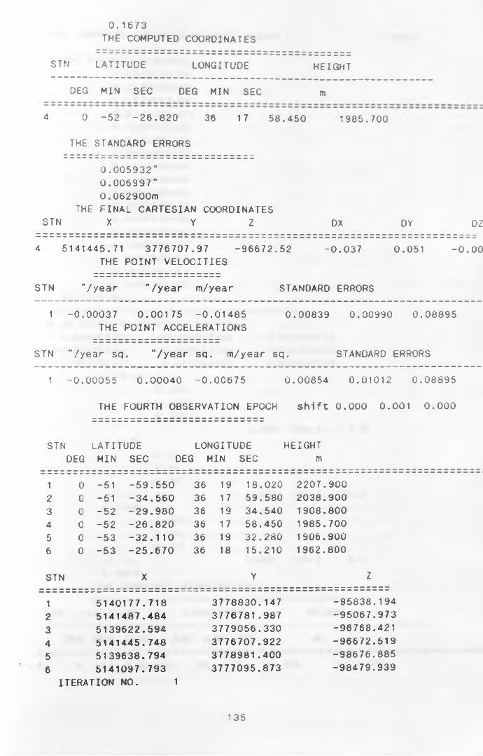
0.1673THE COMPUTED COORDINATES
STN LATITUDE LONGITUDE HEIGHT
DEG MIN SEC DEG MIN SEC m
4 0 -62 -26.820 36 17 58.450 1985.700
THE STANDARD ERRORS
0.005932"0.006997"0.062900m
THE FINAL CARTESIAN COORDINATESSTN X Y Z DX DY DZ
4 5141445.71 3776707 .97 -96672.52 -0.037 0.051 -0.00THE POINT VELOCITIES
STN "/year "/year m/year STANDARD ERRORS
1 -0.00037 0.00175 -0.01485 0,.00839 0.00990 0.08895THE POINT ACCELERATIONS
STN "/year sq "/year sq. m/year sq. STANDARD ERRORS
1 -0.00055 0.00040 -0.00675 0. 00854 0.01012 0.08895
THE FOURTH OBSERVATION EPOCH shift 0.000 0.001 0.000
STN LATITUDE LONGITUDE HEIGHTDEG MIN SEC DEG MIN SEC m
1 0 -51 -59.550 36 19 18.020 2207.9002 0 -51 -34.560 36 17 59.580 2038.9003 0 -52 -29.980 36 19 34.540 1908.8004 0 -52 -26.820 36 17 58.450 1985.7005 0 -53 -32.110 36 19 32.280 1906.9006 0 -53 -25.670 36 18 15.210 1962.800
STN X Y Z
n ii ii n m ii ii n ii ii n n ii ■ iiiniinniiniinn nniinniinniiniiniiniiii ii ii ii n n n n n ii n n ii n ii ii
1 5140177.718 3778830.147 -95838.1942 5141487.484 3776781.987 -95067.9733 5139622.594 3779056.330 -96768.4214 5141445.748 3776707.922 -96672.5195 5139638.794 3778981.400 -98676.8856 5141097.793 3777095.873 -98479.939
ITERATION NO. 1
135

THE COMPUTED VARIANCE OF UNIT WEIGHT= 1 .0 0 0 0THE PARAMETER MATRIX
0.495913E-04 0.223514E-02
-0.133901E-04 0.673132E+01 0.129610E+02 0.4 74246E+01 0.288008E+00 0.427240E+01 0.799852E+00
-0.600489E+00 0.155249E+02
-0.510793E-03 0.156058E-02
-0.149020E-01 -0.593583E-04 0.169835E-02
-0.109419E-01 STATION NO. 4
Q IN LOCAL ELLIPSOIDAL SYSTEM0.025347779 -0.024903745 -0.007902752
-0.024903745 0.034325268 0.011254923-0.007902752 0.011254923 0.039062729
0.2510- 0.866-0.4960.052
1.000 209.8 3.00.0670
-0.0730.022
-0.9971.000 163.0 -85.6
0.1768-0.4940.8680.055
1.000 119.6 3.20.1814
THE COMPUTED COORDINATES
STN LATITUDE LONGITUDE HEIGHT
DEG MIN SEC DEG MIN SEC m
0 -52 -26.820 36 17 58.450 1985.700
136

THE STANDARD ERRORS
0.006433"0.007579"0.068769m
THE FINAL CARTESIAN COORDINATESSTN X Y 2 DX DY DZ
4 5141445.71 THE
3776707.98 -96672 POINT VELOCITIES
.52 0.041 0.056
STN "/year "/year rn/year STANDARD ERRORS
1 -C.00051 THE
0.00156 -0.01490 POINT ACCELERATIONS
0.00914 0.01078 0.09725
STN "/year sq . "/year sq. m/year sq. STANDARD ERRORS
1 -0.00006 0.00170 -0.01094 0.00809 0.00958 0.08422
THE FIFTH OBSERVATION EPOCH -0 52 26.825 36 17 58.453 1985.66C
STN LATITUDE LONGITUDE HEIGHTDEG MIN SEC DEG MIN SEC m
1 0 -51 -59.550 36 19 18.C2C 2207.9002 C _ C 1 -34.560 36 17 59.530 2033.900
r* _ C 9yJ 4. -29.980 36 13 34.540 1908.8004 0 -52 -26.820 36 17 58.450 1985.7005 0 -53 -32.110 36 19 32.280 1906.9006 0 -53 -25.670 36 18 15.210 1962.800
STN X Y Z
1 5140177.718 3778830.147 -95838.1942 5141487.484 3776781.987 -95067.9733 5139622.594 3779056.330 -96768.4214 5141445.748 3776707.922 -96672.5195 5139638.794 3778981.400 -98676.8856 5141097.793 3777095.873 -98479.939
ITERATION NO. 1
THE COMPUTED VARIANCE OF UNIT WEIGHT = 1.0000
THE PARAMETER MATRIX 0.205463E-03 0.247809E-02
-0.721011E-04 0.326110E-01 0.814623E-01
137

THE STANDARD ERRORS
0.006433"0.007579"0.068769m
THE FINAL CARTESIAN COORDINATESSTN X Y 2 DX DY DZ
4 5141445.71THE
3776707.98 -96672 POINT VELOCITIES
.52 0.041 0.056
STN "/year "/year m/year STANDARD ERRORS
1 -C.00051 THE
0.00156 -0.01490 POINT ACCELERATIONS
0.00914 0.01078 0.09725
STN "/year sq . "/year sq. m/year sq. STANDARD ERRORS
1 -0.00006 0.00170 -0.01094 0.00809 0.00958 0.08422
THE FIFTH OBSERVATION EPOCH -0 52 26.825 36 17 58.453 1985.66C
STN LATITUDE LONGITUDE HEIGHTDEG MIN SEC DEG MIN SEC m
1 0 -51 -59.550 36 19 18.020 2207.9002 C -Cl -04.560 36 17 59.530 2033.900•y o _ c o
sJ -29.980 36 19 34.540 1908.8004 0 -52 -26.820 36 17 58.450 1985.7005 0 -53 -32.110 36 19 32.280 1906.9006 0 -53 -25.670 36 18 15.210 1962.800
STN X Y 2
1 5140177.718 3778830.147 -95838.1942 5141487.484 3776781.987 -95067.9733 5139622.594 3779056.330 -96768.4214 5141445.748 3776707.922 -96672.5195 5139638.794 3778981.400 -98676.8856 5141097.793 3777095.873 -98479.939
ITERATION NO. 1
THE COMPUTED VARIANCE OF UNIT WEIGHT= 1.0000
THE PARAMETER MATRIX 0.205463E-03 0.247809E-02
-0.721011E-04 0.326110E-01 0.814623E-01
137

0.44634 7 E+01 -0.3673C4E+00 0.438317E+01
-0.142869E+01 -0.396087E+00 0.162211E+02
-0.66 7 329E-03 0.133612E-02
-0.148415E-01 -0.572049E-03 0.339013E-02
-0.181030E-01 STATION NO. 4
Q IN LOCAL ELLIPSOIDAL SYSTEM0.000295420 -0.000288706 -0.000089633
-0.000288706 0.000397893 0.000127748-0.000089633 0.000127748 0.000454313
0.0270- 0.868-0.4930.053
1.000 209.6 3.10.0073
-0.0740.022
-0.9971.000 163.5 -85.6
0.0191-0.4910.8700.055
1.000 119.4 3.20.0196
THE COMPUTED COORDINATES
STN LATITUDE LONGITUDE HEIGHT
DEG MIN SEC DEG MIN SEC m
4 0 -52 -26.820 36 17 58.450 1985.700
THE STANDARD ERRORS
0.000694”0.000816”0.007472m
THE FINAL CARTESIAN COORDINATES STN X Y Z DX
4 5141445.70 3776707.98 -96672.51 -0.045
DY
.062

THE POINT VELOCITIES
STN "/year "/year m/year STANDARO ERRORS
1 -0.00067 0.00134 -0.01484 0.00099 0.00117 0.01057THE POINT ACCELERATIONS
STN "/year sq. "/year sq. m/year sq. STANDARD ERRORS
1 -0.00057 0.00339 -0.01810 0.00083 0.00098 0.00863
139

Appendix C.4 Results for the 5th epoch observations -static mode
APPROX. COORDINATES
STN LATITUDE LONGITUDE HEIGHTDEG MIN SEC DEG MIN SEC m
1 -51 -59 .550 36 19 18..020 2207..9004* 0 -51 -34 .560 36 17 59..580 2038..9003 0 -52 -29 . 980 36 19 34 ..540 1908., 8004 0 -52 -26 .820 36 1 7 58..450 1985.,7005 0 -53 -32 .110 36 19 32.,280 1906.,9006 0 -53 -25 .670 36 18 15.,210 1962.,800
STN X Y Z
1 5140 177. 718 3778830. 147 -958382 5141 487.-484 3776781. 987 -95067,3 5139622.5944 5141445.7485 5139638.7946 5141097.793
ITERATION NO.
377905637767073778981
330922400
3777095.873
-96768.421-96672.519-98676.885-98479.939
THE COMPUTED VARIANCE OF UNIT WEIGHT=ITERATION NO. 1
THE COMPUTED VARIANCE OF UNIT WEIGHT= ITERATION NO. 2
THE COMPUTED VARIANCE OF UNIT WEIGHT= POTENTIAL DIFFERENCE
RESIDUAL SCALED WEIGHTS
-0.002141112 0.292826 7E+06-0.002798314 0.2928267E+06-0.000376274 0.2928267E+06-0.000327732 0.2928267E+060.001515449 0.2928267E+06
-0.002112975 0.2928267E+060.002170707 0.2928267E+06
-0.000288810 0.2928267E+060.002276538 0.2928267E+060.000167338 0.2928267E+060.001170601 0.2928267E+060.000341433 0.2928267E+060.002566614 0.2928267E+060.000364097 0.2928267E+06
119.2633
1.0002
1.0000
140

-0.C01017982 0.2928267E+06-0.001214829 0.292826 7E+06-0.000065728 0.292826 7E+060.002692556 0.2928267E+06
-0.002206315 0.2928267E+06-0.000021611 0.2928267E+06-0.001298766 0.2928267E+06-0.003082253 0.2928267E+06-0.000178538 0.2928267E+060.0011y4223 0.2928267E+06
VTVP TRACE SIG USED % LEFT % TOTAL 08S
19.00967 19.00967 1.000000 20.79 79.21 244.99 19.01
GRAVITY DIFFERENCE
LATITUDE
RESIDUAL SCALED WEIGHTS
0.000433501 0.5916228E+050.000097484 0.5916238E+05
-0.000150904 0.5916238E+050.000621908 0.5916238E+050.000006709 0.5916238E+05
-0.000000554 0.5916238E+05VTVP TRACE SIG USED % LEFT % TOTAL OBS
0.03591 0.03591 1.000000 99.40 0.60 65.96 0.04
LONGITUDE
RESIDUAL SCALED WEIGHTS
-0.001619188 0.2331721E+05-0.000142556 0.2331721E+050.000486859 0.2331721E+050.000017785 0.2331721E+05
-0.000207360 0.2331721E+050.000000108 0.2331721E+05
VTVP TRACE SIG USED % LEFT % TOTAL OBS
0.06814 0.06814 1.000000 98.86 1.14 65.93 0.07
AZIMUTH
RESIDUAL SCALED WEIGHTS
iiiiniiiinniiniiniiniiniiniiiiiiii n n ii ii ii n ii ii n ii ii ii n =====-3.349599301 0.6928144E-01-3.755113928 0.6928144E-01
VTVP TRACE SIG USED % LEFT * TOTAL OBS
141

1.75425 1.75425 1.000000 12.29 87.71 20.25 1.75
VERTICAL ANGLES
RESIDUAL SCALED WEIGHTS
-3.286040215 0.6820665E-016.871615350 0.6820665E-01
-2.774655704 0.6820665E-013.367876561 0.6820665E-01
-1.254831247 0.6820665E-011.363452839 0.6820665E-012.213275561 0.6820665E-01
-6.633695116 0.6820665E-013.224673771 0.6820665E-01
-2.211899384 0.6820665E-01VTVP TRACE SIG USED % LEFT % TOTAL CBS
9.86867 9.86867 1.000000 1.31 98.69 100.13 9.87
SPATIAL DISTANCES
RESIDUAL SCALED WEIGHTS
0.005110717 0.8287340E+050.002220210 0.27955 70E+U6
-0.001069531 0.7964854E+05-0.001695841 0.6635895E+U50.004833152 0.8287342E+05
-0.004243007 0.4958516E+050.001598575 0.1735993E+060.002355428 0.4823927E+050.002108212 0.2795570E+06
-0.005737938 0.4958521E+05-0.000081456 0.6315408E+050.002455046 0.1337917E+06
-0.001257973 0.7964856E+050.001099738 0.1735994E+06
-0.000060191 0.6315408E+05-0.002615317 0.4623641E+05-0.003199296 0.1370578E+06-0.001468222 0.6635894E+050.002644871 0.1337916E+06
-0.002256245 0.4623640E+050.000663130 0.9248664E+050.000446361 0.6250105E+05
-0.002495673 0.1370577E+060.000732916 0.9248663E+05
142

VTVP TRACE SIG USED % LEFT * TOTAL 082
15.42075 15.42075 1.000000 35.75 64.25 248.58 15.42
HORIZONTAL ANGLES
RESIDUAL SCALED WEIGHTS
3.887806217 0.3267808E-015.988433892 0.3267808E-01
-11.282736542 0.3267808E-011 .240950812 0.3267808E-012.476789219 0.3267808E-011.730231188 0.3267808E-01
-2.428832706 0.3267808E-01-1.720254942 0.3267808E-010.877918862 0.3267808E-015.474905426 0.3267808E-01
-7.935941697 0.326 7 808E-011.790696897 0.3267808E-01
-5.354395844 0.3267808E-016.431937560 0.326 7 808E-01
-3.143935201 0.3267808E-010.275145846 0.3267808E-011.096713229 0.3267808E-010.747392590 0.3267808E-01
-0.287696825 0.3267808E-01-6.906005938 0.326 7 808E-015.902223708 0.326 7 808E-011.931485871 0.3267808E-01
-5.863235880 0.3267808E-014.265538065 0.3267808E-01
VTVP TRACE SIG USED % LEFT % TOTAL OBS
16.84261 16.84261 1.000000 29.827.16
70.1816.84
24
TOTAL DEGREES OF FREEDOM = 63.000
THE PARAMETER MATRIX 0.220787E-02 0.251431E-02 0.686813E-02 0.213882E-02 0.199689E-03 0.658815E-02
-0.555428E-03 -0.873539E-03 0.650018E-02 0.290186E-03
143

0.780316E-02 -0.333338E-01 -0.5 75273E-04 0.172115E-03 0.668253E-02
-0.400984E-02 -0.97 3674E-02 0.669465E-02
-0.990954E-01 0.573519E-01
-0.126818E-01 0.294236E-01 0.318926E-01
-0.510808E-01 -0.549894E-01 -0.308006E-01 0.259972E-02
-0.762330E-03 0.319878E-01
-0.702656E-03 -0.273208E+01 -0.105534E+01 -0.668494E+01 -0.134454E+02 -0.375114E+01 -0.161323E+01
STATION NO. 1
Q FOR PHI, LAMBDAfH 0.000000053 0.0000000090.000000009 0.000000093
-0.000000021 -0.0000000550 IN LOCAL ELLIPSOIDAL SYSTEM
0.000034695 -0.000041765-0.000041765 0.000057488-0.000005095 0.000007036
0.0096-0.978-0.2070.020
0 . 0017-0.019- 0 .0 1 0-1.000
- 0.000000021-0.0000000550.000002837
-0.0000050950.0000070360.000050133
1.000 191.9
1.000 208.9
-0.2070.978
-0.006
0 . 0 0 6 9
1 .0 0 0 1 0 1 .9
144
1.2
8 8 . 8
- 0 . 4

0.0069STATION NO. 2
0 FOR PHI, LAMBDA,H 0.000000149 0.0000000470.000000047 0.000000066
-0.000000006 -0.0000000770 IN LOCAL ELLIPSOIDAL SYSTEM
0.000025744-0.000028902-0.000025121
0.0127
0.0018
0.0065
0.0083 STATION NO.
-0.0000289020.0000402900.000037371
-0.416-0.9090.007
-0.0520.016
-0.999
-0.9080.4160.053
-0.000000006-0.0000000770.000003237
-0.0000251210.0000373710.000140384
1.000 245.4
1.000 163.2
1.000 155.4
Q FOR PHI, LAMBDA,H 0.000000065 -0.000000020
-0.000000020 0.000000064-0.000000005 -0.000000042
Q IN LOCAL ELLIPSOIDAL SYSTEM 0.000024612 -0.000028561
-0.000028561 0.0000390910.000012114 -0.000015212
0.00900.711
-0.703- 0 . 011
-0.000000005-0.0000000420.000002421
0.000012114-0.0000152120.000060867
1.000 315.30.0015
-0.026 - 0 . 0 1 1 - 1 .0 0 0
1.000 203.1
0.7030.711
-0.026
0 .0 0 6 5
145
0.4
86.9
3.1
- 0.6
88.4

1.000 45.3 -1.50.0064
. - I O N NO. 4
^ PHI, LAMBDA ,H U * , .ju 0 00063 -0.000000015
^ g O O O O 0 1 5 0.000000057j J 0 0 0 0 0 0 4 -0.000000049
-V< u O C A L ELLIPSOIDAL SYSTEM___'62 -0.000025609
’ j J O O 2 5 6 0 9 0.000034654* j j u 0 0 9 1 9 3 -0.000011260
O .00850.647
-0.763-0.013
O .0015-0.032- 0 .0 1 0-0.999
O .00650.7620.647
-0.031
-0.000000004-0.0000000490.000002159
0.000009193-0.0000112600.000059604
1.000 310.3
1.000 198.0
1.000 40.3
^ » j . O H
O .0062 NO. 5
I- O R PHI, LAMBDA,H . 0 0 0 0 0 0 1 3 8 0.000000039
u . U O O U G 0 0 3 9 0.000000064J - O U U O O O O O O -0.0000000611 l o c a l ellipsoidal system u - 0 0 0 0 2 4 5 5 9 -0.000028237° • 0 0 0 0 2 8 2 3 7 0.000039501<J * O 0 0 0 2 0 5 9 4 0.000031337
O.0121-0.401-0.9160.005
O.0017-0.039
0.011-0.999
-0.9150.401
0.0067
0.000000000-0.0000000610.000002820
-0.0000205940.0000313370.000130358
1.000 246.4
1.000 163.8 -
-0.7
88.1
- 1.8
0.3
87.7
146

0.041
0.0081 STATION NO.
1.000 156.4 2.3
O FOR PHI, LAMBDA,H 0.000000058 0.0000000210.000000021 0.0000001540.000000000 -0.000000086
Q IN LOCAL ELLIPSOIDAL SYSTEM 0.000056472 -0.000069359
-0.000069359 0.000094991-0.000010949 0.000016224
0.0123-0.980-0.1980.018
0.0019-0.0190.007
- 1 .000
0.0071-0.1970.9800.011
0.000000000-0.0000000860.000003775
-0.0000109490.0000162240.000054792
1.000 191.4 1.0
1.000 159.6 -88.8
1.000 101.4 0.60.0083
THE COMPUTED COORDINATES
STN LATITUDE LONGITUDE HEIGHT
DEG MIN SEC DEG MIN SEC m— ======= n i i z i =============== ============= ============ Z Z Z Z Z Z
1 0 -51 -59.548 36 19 18.022 2207.9072 0 -51 -34.558 36 17 59.582 2038.9073 0 -52 -29.981 36 19 34.543 1908.8074 0 -52 -26.820 36 17 58.459 1985.6675 0 -53 -32.110 36 19 32.281 1906.9076 0 -53 -25.674 36 18 15.211 1962.807
THE FINAL CARTESIAN COORDINATESSTN X Y Z DX DY
1 5140177.68 3778830.21 -95838.13 -0.040 0.067
2 5141487.49 3776782.00 -95067.91 0.002 0.009
3 5139622.61 3779056.31 -96768.44 0.021 -0.018
4 5141445.58 3776708.10 -96672.51 -0.170 0.175
5 5139638.80 3778981.41 -98676.89 0.002 0.008
6 5141097.98 3777095.63 -98480.06 0.182 -0.240
DZ
0.0620.066
-0.0170.009
- 0.00-0.12
147
to
ro

r e f e r e n c e s
1 • Aduol , F.W.O., 1981: Optimal design for a
three-dimensional terrestrial geodetic network. Thesis
submitted for the Degree of blaster of Science (Surveying) in the University of Nairobi.
2. Aduol, F.W.O., 1989: Integriete geodatische Netzanalyse
mit s t ochastischer vorinformation uber schwerefeld und
ref e r e n z e i i i psoi d . Deutsche Geoctxti sche Kommission Nr C-351 , M u n c h e n 1989.
3. A d u o l , F.W.O., and Schaffrin, B., 1990: Geodetic models
f o r monitoring crustal deformation along the African Rift
S y s t e m . IASPEI/UNESCO/ICL Regional Seismological Assembly in
A f r i c a . Nairobi, 22-29 August, 1990.
4. A d u o l , F.W.O., 1990: Lecture Notes funpublished). Class
n o t e s f o r course FSP 401, Dept. Surveying & Photo. U.o.N.
5. A s h k e n a z i , V., and Dodson, A.H., 1980: Ground movements
and structures. Proceedings of the 2nd. Intern, conference
h e l d a t t he University of Wales Institute of Science and
J e c h n o l o g y . Cardiff, April 1980.
6- Ashkenazi, V., and Grist, S.N., 1983: 3-D geodetic network
adjustment models: Significance of different approaches.
P r o c . of the IAG Symposia, V o l . 2 , August 15-27, 1983.
7- B i a c s , F.Z., andTeskey, W.F., 1990: A PC-Based program
system for adjustment and deformation analysis of precise
e n 9i n e e r ing and monitoring networks. Aust. journal.
Geodesy Photogrammetry and Surveying. No. 52 June 1990 . pp
148

37-55.
8. Bjerhammer, A., 1973: Theory of errors and generalized
matrix inverses, Elsevier, Amsterdam.
9. Bomford, G., 1980: Geodesy. 4th edition, Claredon Press,
Oxford.
10. Brunner, F.K., 1979: On the analysis of geodetic networks
for the determination of the incremental strain tensor.
Survey review.XXV, 192, April 1979. pp 56-67
11. Caspary, W. , 1988: A robust approach to estimating
deformation parameters. Proc. of the 5th International
Symposium on Deformation Measurements, Fredericton, Canada,
June pp. 124-135.
12. Chen, Y.Q., Kavouras, M., and Secord, J.M., 1983: Design
considerations in deformation monitoring. Proceedings, 17th
Congress, Federation Internationale des Geometres, Commission
6, Paper 608.2, Sofia.
13. Chen, Y.Q., Chrzanowski, A., and Secord, J.M., 1990: A
strategy for the analysis of the stability of reference
points in deformation surveys. CISM Journal ACSGC. Vol. 44,
No. 2, Summer 1990. pp. 141 to 149.
14. Cooper, M.A.R., 1987: Control Surveys in Civil
Engineering. Collins Professional and lechnical books.
William Collins & Sons Co. Ltd. ( Grafton Street, London W1X
3LA.
15. Crosilla, F., and Marchesini, C., 1986: Geodetic control
network in Friuli (Caneva, PN): First results. Seminar Paper
149

on Modern trends in deformation measurements'.bolgna,
Instituto di Topografia, Geodesia e Geofisica Mineraria 26-27
giugno 1986.
16. Cross, P.A., 1979: Geodesy Lecture notes ("unpublished).
Dept, of Surveying & Photogrammetry, Univ. of Nairobi.
17. Davies, M.J.K., Proctor, D.W., Ashkenazi, V. and Cross,
P.A., 1971: The readjustment of the retriangulation of Great
Britain, and its relationship to the European terrestrial and
satellite networks. Proc.of the conference of commonwealth
survey officers, Cambridge.
18. Drew, A.R., and Snay, A.R., 1988: Supplementing geodetic
data with priori information for crustal deformation in the
Imperial Valley, California. Technical Report No. 6,
Institute of Geodesy, University of Stuttgart.
19 Forster, T.A., 1990: Engineering classification of
movement probability related to deformation survey 95%
confidence ellipses and limits.New Zealand Surveyor, Vol .
XXXIII, No.277
20 Grafarend, E.W., 1974: Optimisation of geodetic networks.
The Canadian Surveyor, 28(5), 716-723.
21 Grafarend, E.W., 1988: Azimuth transport and the problem
of orientation within geodetic traverses and geodetic
networks. Vermessung Photogrammetrie Kulturtechnick 7/88 pp.
315-332.
22. Grafarend, E.W., and Richter, B., 1978: Three dimensional
geodesy II - the datum problem ZPV, Feb. 1978. pp. 44-59. 22.
150

23. Grafarend, E.W., and Schaffrin, B., 1974: Unbiased
Freenet adjustment. Survey Review. XXII, 171, January 1974.
24. Grundig, L., Neureither, M., and Bahndorf, J., 1985:
Detection and localization of geometrical movements. Journal
of Surveying, Vol. Ill, No.2, August, 1985. pp. 119-132.
25. Heiskanen, W.A., and Moritz, H., 1967: Physical Geodesy .
W.H Freeman and Company, San Franscisco 1967.
26. Flirvonen, R.A., 1971: Adjustment by least squares in
Geodesy and Photogrammetry. Frederick Ungar Publishing Co.
New York.
27. Flradilek, L., 1985: Three-dimensional terrestrial
triangulation. Konrad Wittwer Verlag, Stutgart.
28. Illner, I., 1985: Datumsfestlegung in freien Netzen.
Deutsche Geocktische Kommission. Reihe C Fleft Nr.309. pg. 9.
29. Kelly, I., 1983: Monitoring Surveys at Loy Yang.
Symposium on the surveillance of engineering structures,
University of Melbourne.
30. Koch, K.R, 1988. Parameter Estimation and Hypothesis
Testing in Linear Models. Springer-Verlag. Berlin Heidelberg.
31. Koch, K.R., and Fritsch, D., 1981: Multivariate
hypothesis tests for detecting recent crustal movements.
Tectonophysics, 71(1981) 301-313. Elsevier Scientific
publishing Co., Amsterdam.
32. McConnel, R.K., Hearty, D.B. and Winter, P.J., 1975: An
evaluation of the Lacoste- Romberg model D Microgravimeter.
151

Bureau Gravim. Intern., Bull. d ’Inform, no. 36.
33. Meissl, P., 1982: Least squares adjustment. A modern
approach. Mittellungen der geodatischen Institute der
Technischen Universitat, Craz. Folge 43.
34. Mikhail, E.M., 1976: Observations and least squares.
(Reprint). University Press of America. Lanham. New York.
London.
35. Mittermayer, E., 1972: "A generalization of least squares
adjustment of free networks". Bull. Geoid., No.104, pp
139-155
36. Mueller, I.I., and Ramsayer, K.H., 1979: Introduction to
Surveying. Frederick Ungar Publishing Co. /New York.
37. Murnane, A.B., 1983: Monitoring Surveys at Winneke
Reservoir- Aspects of network design and analysis. Proc.
Symposium on the surveillance of Engineering Structures,
Dept, of Surveying, Univ. of Melbourne.
38. Niemeier, W. , 1981: Statistical tests for detecting
movements in repeatedly measured geodetic networks.
Tectonophysics, 71(1981) 335-351. Elsevier Scientific
Publishing Co. Amsterdam.
39. Niemeier, W., 1985: Netzqualitat und Optmierung. In H.
Pelzer (Ed); Geoc&tische Netze in Landes-Und
Ingenieurvermessung I. Konrad Wittwer, Stuttgart 1985, pp.
153-224
40. Papo, H.B., and Perelmuter, A., 1984: Pre zero epoch
covariance matrix in sequential analysis of deformations.
152

Bulletin Geodesique. Vol. 56 No. 1
41. Pelzer, H., 1977: Criteria for the reliability of
geodetic networks. Proc. International Symposium on
Optimisation of Design and Computations of Geodetic Networks,
Sopron.
42. Perelmuter, A., 1979: Adjustment of free networks.
Bulletin Geodesique No. 4, Vol.53.
43. Rapp, R.H., 1982: A FORTRAN program for the computation
of gravimetric quantities from high degree spherical harmonic
expansions. Reports of the Dept, of Geodetic Science and
Surveying. Report No. 334. The Ohio State University 1958
Neil Avenue, Columbus, Ohio 43210.
44. Richardus, P., 1966: Project Surveying. North-Hoi 1 and
publishing Co. Amsterdam.
45. Robbins, A.R., 1976: Field and Geodetic Astronomy.
Military Engineering, Vol. 13. Part 9 U.K. Ministry of
Defense.
46. Rueger, J.M., 1983: Reduction of Mekometer measurements.
School of Surveying, Univ. of New South Wales.
47. Schaffrin, B. 1984: Aspects of network design. In:
Grafarend, E.W., Sanso F (Eds); Optimisation and design of
geodetic networks. Spring-Ver1ag, Berlin-Heidelberg- New York
-Tokyo 1985; pp.548-597
48. Schmitt, G., 1990: Lecture notes (unpublished) for course
FSP 402. Dept, of Survey & Photo., University of Nairobi.
153

4-9. Stolz, A., 1972: "Three dimensional cartesian coordinates
of part of the Australian network by the use of local
astronomic vector systems". Unisurv Report. No. 58, Univ. of
New South Wales, Sydney.
50. Shortis, M.R., 1983: Deformation analysis and monitoring
by close range analytical photogrammetry. Symposium on the
Surveillance of engineering structures. University of
Mel bourne.
51. Torge, W., 1980: Geodesy. Walter de Gruyter. Berlin. New
York.
52. Torge, W., 1986: Gravimetry for monitoring vertical
crustal movements: Potential and problems. Tectonophysics,
130: 385-393; Amsterdam.
53. van Mierlo, J., 1975: Statistical analysis of geodetic
networks designed for the detection of crustal movements. In:
Progress in Geodynamics- North- Holland Publ. Comp.
Amsterdam/ New York.
54. van Mierlo, J., 1975(a): Testing and adjusting 2- and
3-dimensional networks for detecting deformation
measurements, Krakow.
55. van Mierlo, J., 1981: A testing procedure for analysing
geodetic deformation measurements. Proc. , 2nd International
Symposium of Deformation Measurements by geodetic methods.
Bonn, 1978 (ed.L Hallermann) pp. 321-353.
154