Embed Size (px)
Citation preview
UNIVERSITY COLLEGE LONDON
DOCTORAL THESIS
Mathematical Modelling of CleanWater Treatment Works
Folashade AKINMOLAYAN
A thesis submitted in ful�llment of the requirements
for the degree of Doctor of Philosphy
in the
Centre for Process Systems Engineering
Department of Chemical Engineering
2017

I, Folashade AKINMOLAYAN, con�rm that the work presented in this thesis is my own.
Where information has been derived from other sources, I con�rm that this has been
indicated in the thesis.
Signature
Date
i

Acknowledgements
Through the years, I met so many wonderful people I am thankful for seeing me through
this journey. Firstly, I would like the thank Professor Eva Sorensen for guiding a nervous
student. You have played so many important roles in my life, initially a supervisor, a
line manager, a friend and a constant shoulder to cry on. Thank you for correcting me
when I was wrong (spelling and grammar especially), supporting me when I was right,
and taking time out of your own life to ensure I did not procrastinate. You have help
mould me into the woman I have become today and I am beyond grateful our paths
crossed. I am grateful to my secondary supervisor Professor Nina Thornhill for all the
interesting discussions and your eye for details.
To the close friends before this journey: Gurbinder, Sa�e, Folake, Beverley, Mickal,
Bianca, Sara, Na�sah, Belquis, �The Lous�, Vidal and Carl.
To the friends I met along the way: Rema, Matt, Mithila, Ishanka, Chara, Noor,
Matteo, George and Alex.
You have all played a crucial role in this chapter of my life.
To Eria and Vivien, thank you for the long distance encouragement and entertainment.
To my �lovely ladies� lunch club: Emanuela, Kate, and Elpida thank you for your
continued words of wisdom and encouragement.
Vassilis and Asif, you both are my PPSE best friends who always kept me laughing.
You both understood the pains and joys of computer modelling. Thank you for your
continued support and random adventures.
Above all I wish to thank my parents, siblings and nephews for their faith in me, their
unconditional love, their endless support and understanding throughout all these years.
None of this would be possible without them and to them I am eternally grateful.
Special mentions go to my dad and my brother Ore for taking care of me when I
neglected to take care of myself, for the sweet treats when I craved them but mostly
for being there to kill the spiders whenever I needed them no matter the time of night.
Dami - thank you for your constant love, motivation, encouragement, Thai food and
patience at all times. We shared this PhD journey together and you always cheered
me up, stood by me through the good, bad and the panic because I could not solve an
�error� in my code.
ii

Abstract
One of the biggest operational risks to water companies arises from their ability to
control the day-to-day management of their water treatment plants. With increasing
pressures to remain competitive, companies are looking for solutions to be able to make
predictions on how their treatment processes can be improved. This work focuses on
mathematical modelling and optimisation of clean water treatment processes. The main
motivation is to provide tools which water companies can use to predict the performance
of their plants to enable better control of risks and uncertainties.
Most modelling work within water operations has so far been based on empirical
observations rather than on mathematically describable relationships of the process as
will be considered in this work. Mathematical models are essential to describe, predict
and control the complicated interactions between the di�erent parts of the treatment
process, a concept which is well understood within the process industry but not yet
established within the water treatment industry. This work will also consider the level
of modelling detail actually required to accurately represent a water treatment plant.
This thesis develops the conceptual understanding of clean water treatment processes
utilising �rst principles modelling techniques. The main objective of this work is
the consideration of a complete mathematical model of an entire water treatment
plant, which enables a wider view on how changes in one processing unit will a�ect
the treatment process as a whole. The performance of the process models are �rst
veri�ed individually and are then combined to enable the simulation of a complete water
treatment work. By using detailed modelling (especially gPROMS utilised in this work)
requires specialist software knowledge. Without knowledge of advanced simulation tools
or having a background in process modelling, the detailed models developed in this
work would not be fully utilised if implemented in the water industry, if utilised at
all. A systematic framework is presented for the development of simpler surrogate
models that can be used to predict the e�uent suspended solids concentration, for a
given number of independent variables. This approach can provide valuable guidance
in clean water treatment process design and operation, thus providing a tool to achieve
better day-to-day performance management.

My thesis in a drop.

Contents
Declaration of Authorship . . . . . . . . . . . . . . . . . . . . . . . . . . i
Acknowlegdements . . . . . . . . . . . . . . . . . . . . . . . . . . . . . . . ii
Abstract . . . . . . . . . . . . . . . . . . . . . . . . . . . . . . . . . . . . . iii
List of Figures . . . . . . . . . . . . . . . . . . . . . . . . . . . . . . . . . xiv
List of Tables . . . . . . . . . . . . . . . . . . . . . . . . . . . . . . . . . . xviii
List of Notation . . . . . . . . . . . . . . . . . . . . . . . . . . . . . . . . xxiii
1 General introduction 1
1.1 Scope . . . . . . . . . . . . . . . . . . . . . . . . . . . . . . . . . . . . 1
1.2 Water Industry: raw water . . . . . . . . . . . . . . . . . . . . . . . . 4
1.2.1 Raw water sources . . . . . . . . . . . . . . . . . . . . . . . . . 5
1.3 Clean water treatment process . . . . . . . . . . . . . . . . . . . . . . . 7
1.4 Motivation . . . . . . . . . . . . . . . . . . . . . . . . . . . . . . . . . . 10
1.5 Objectives and contributions of this thesis . . . . . . . . . . . . . . . . 13
1.6 Organisation of this thesis . . . . . . . . . . . . . . . . . . . . . . . . . 13
v

CONTENTS vi
2 Literature review 15
2.1 Introduction . . . . . . . . . . . . . . . . . . . . . . . . . . . . . . . . 15
2.2 What is Process Systems Engineering (PSE)? . . . . . . . . . . . . . . 16
2.2.1 Fundamentals and methodologies of PSE . . . . . . . . . . . . 17
2.2.2 Enterprise-wide optimisation . . . . . . . . . . . . . . . . . . . . 20
2.3 Mathematical modelling - clean water industry . . . . . . . . . . . . . . 21
2.3.1 Turbidity vs. Suspended solids concentration . . . . . . . . . . 23
2.3.2 Coagulation and �occulation . . . . . . . . . . . . . . . . . . . 24
2.3.3 Clari�cation . . . . . . . . . . . . . . . . . . . . . . . . . . . . 33
2.3.3.1 Flotation tank studies . . . . . . . . . . . . . . . . . . 43
2.3.4 Filtration . . . . . . . . . . . . . . . . . . . . . . . . . . . . . . 48
2.3.4.1 One-dimensional modelling . . . . . . . . . . . . . . . 51
2.3.5 Disinfection . . . . . . . . . . . . . . . . . . . . . . . . . . . . . 59
2.3.5.1 Kinetic model . . . . . . . . . . . . . . . . . . . . . . . 60
2.4 Challenges and opportunities . . . . . . . . . . . . . . . . . . . . . . . 65
2.5 Overall concluding remarks . . . . . . . . . . . . . . . . . . . . . . . . 66
2.6 Conclusions . . . . . . . . . . . . . . . . . . . . . . . . . . . . . . . . . 68
3 Modelling of clean water treatment units 70
3.1 Introduction . . . . . . . . . . . . . . . . . . . . . . . . . . . . . . . . . 70
3.2 Modelling of coagulation and �occulation . . . . . . . . . . . . . . . . . 71
3.2.1 Unit principle . . . . . . . . . . . . . . . . . . . . . . . . . . . 71
3.2.2 Model development . . . . . . . . . . . . . . . . . . . . . . . . 72

CONTENTS vii
3.2.3 Numerical simulation and validation . . . . . . . . . . . . . . . 80
3.2.4 Concluding remarks . . . . . . . . . . . . . . . . . . . . . . . . . 85
3.3 Modelling of clari�cation process . . . . . . . . . . . . . . . . . . . . . 85
3.3.1 Unit principle . . . . . . . . . . . . . . . . . . . . . . . . . . . 86
3.3.2 Model development . . . . . . . . . . . . . . . . . . . . . . . . 86
3.3.3 Model simulation and validation . . . . . . . . . . . . . . . . . . 90
3.3.4 Concluding remarks . . . . . . . . . . . . . . . . . . . . . . . . . 93
3.4 Modelling of �ltration . . . . . . . . . . . . . . . . . . . . . . . . . . . 94
3.4.1 Unit principle . . . . . . . . . . . . . . . . . . . . . . . . . . . 94
3.4.2 Model development . . . . . . . . . . . . . . . . . . . . . . . . 94
3.4.3 Model simulation and validation . . . . . . . . . . . . . . . . . 102
3.4.4 Concluding remarks . . . . . . . . . . . . . . . . . . . . . . . . . 107
3.5 General discussion of model development . . . . . . . . . . . . . . . . . 107
3.6 Conclusion . . . . . . . . . . . . . . . . . . . . . . . . . . . . . . . . . . 108
4 Complete model of clean water treatment 110
4.1 Introduction . . . . . . . . . . . . . . . . . . . . . . . . . . . . . . . . . 110
4.2 Unit con�gurations . . . . . . . . . . . . . . . . . . . . . . . . . . . . . 111
4.2.1 Integration of units . . . . . . . . . . . . . . . . . . . . . . . . . 111
4.3 Overall plant performance . . . . . . . . . . . . . . . . . . . . . . . . . 113
4.3.1 Scenario 1 . . . . . . . . . . . . . . . . . . . . . . . . . . . . . . 113
4.3.2 Scenario 2 . . . . . . . . . . . . . . . . . . . . . . . . . . . . . . 118
4.3.3 Scenario 3 . . . . . . . . . . . . . . . . . . . . . . . . . . . . . . 122
4.4 Computational statistics . . . . . . . . . . . . . . . . . . . . . . . . . . 128
4.5 Conclusion . . . . . . . . . . . . . . . . . . . . . . . . . . . . . . . . . . 129

CONTENTS viii
5 Surrogate models for process integration 131
5.1 Introduction . . . . . . . . . . . . . . . . . . . . . . . . . . . . . . . . . 131
5.2 Surrogate modelling . . . . . . . . . . . . . . . . . . . . . . . . . . . . . 132
5.2.1 Arti�cial neural network . . . . . . . . . . . . . . . . . . . . . . 133
5.2.2 Polynomial response surface methodology . . . . . . . . . . . . 134
5.2.3 Full factorial design . . . . . . . . . . . . . . . . . . . . . . . . . 135
5.3 Coagulation-�occulation surrogate model . . . . . . . . . . . . . . . . . 137
5.3.1 Results and validation . . . . . . . . . . . . . . . . . . . . . . . 143
5.3.2 Concluding remarks . . . . . . . . . . . . . . . . . . . . . . . . . 150
5.4 Clari�cation surrogate model . . . . . . . . . . . . . . . . . . . . . . . . 150
5.4.1 Results and validation . . . . . . . . . . . . . . . . . . . . . . . 154
5.4.2 Concluding remarks . . . . . . . . . . . . . . . . . . . . . . . . . 160
5.5 Filtration surrogate model . . . . . . . . . . . . . . . . . . . . . . . . . 161
5.5.1 Results and validation . . . . . . . . . . . . . . . . . . . . . . . 164
5.5.2 Concluding remarks . . . . . . . . . . . . . . . . . . . . . . . . . 167
5.6 Disinfection surrogate model . . . . . . . . . . . . . . . . . . . . . . . 167
5.6.1 Results and validation . . . . . . . . . . . . . . . . . . . . . . . 171
5.6.2 Concluding remarks . . . . . . . . . . . . . . . . . . . . . . . . . 177
5.7 Conclusion . . . . . . . . . . . . . . . . . . . . . . . . . . . . . . . . . . 179

CONTENTS ix
6 Conclusions and recommendations 180
6.1 Review of project deliverables . . . . . . . . . . . . . . . . . . . . . . . 180
6.1.1 Critical assessment of the current state-of art . . . . . . . . . . 181
6.1.2 Dynamic modelling of conventional clean water treatment work 181
6.1.3 Surrogate model development of clean water treatment work . . 183
6.1.4 Concluding remarks . . . . . . . . . . . . . . . . . . . . . . . . . 183
6.2 Direction for future research . . . . . . . . . . . . . . . . . . . . . . . . 184
6.2.1 Use of numerical simulation tools in drinking water treatment . 184
6.2.2 Plant optimisation . . . . . . . . . . . . . . . . . . . . . . . . . 186
6.2.3 Model calibration . . . . . . . . . . . . . . . . . . . . . . . . . . 189
6.2.4 Broader recommendations . . . . . . . . . . . . . . . . . . . . . 190
6.3 Summary and main contributions . . . . . . . . . . . . . . . . . . . . . 191
List of Communications . . . . . . . . . . . . . . . . . . . . . . . . . . . 194
A 219
A.1 General introduction . . . . . . . . . . . . . . . . . . . . . . . . . . . . 219
A.1.1 Water quality regulations . . . . . . . . . . . . . . . . . . . . . 219
B 222
B.1 Modelling the conventional clean water treatment process units . . . . 222
B.1.1 Modelling coagulation and �occulation unit . . . . . . . . . . . 222
C 224
C.1 Implementation of SST model . . . . . . . . . . . . . . . . . . . . . . . 224
C.1.1 Approximation of convective �ux . . . . . . . . . . . . . . . . . 224

List of Figures
1.1 Breakdown of the water availability in the world. . . . . . . . 2
1.2 Public water supply, England and Wales . . . . . . . . . . . . . 3
1.3 EU per capita water consumption (DEFRA, 2014). . . . . . . 4
1.4 Illustration to show how water enters the unsaturated zone
(soil moisture) and the saturated zone (groundwater) (Envi-
ronment and Climate Change Canada, 2013). . . . . . . . . . 6
1.5 Illustration to show an artesian well, which has been drilled
into a con�ned aquifer, and a water table well. The brown
layer represents an �impermeable layer� (Environment and
Climate Change Canada, 2013). . . . . . . . . . . . . . . . . . . 7
1.6 Main technologies available for water treatment processes. . 8
2.1 Graphical representation of the modelling process. Adapted
with permissions from Sargent (2005). . . . . . . . . . . . . . 19
2.2 Integrated framework for PSE in a clean water treatment
plant. . . . . . . . . . . . . . . . . . . . . . . . . . . . . . . . . . 21
2.3 Typical process diagram for clean water treatment plant (with
examples of variations). . . . . . . . . . . . . . . . . . . . . . . 22
2.4 Possible particle collision trajectories. (a) Rectilinear model.
(b) Curvilinear model. Adapted with permissions from Han
and Lawler (1992). . . . . . . . . . . . . . . . . . . . . . . . . . 27
x
LIST OF FIGURES xi
2.5 Cross-section of solid-contact clari�er (AWWA Committee
Report, 1951). . . . . . . . . . . . . . . . . . . . . . . . . . . . . 35
2.6 Schematic overview of an ideal one-dimensional clari�er. Adapted
with permissions from Burger et al. (2011). . . . . . . . . . . 39
2.7 Schematic overview of a dissolved air �otation unit. . . . . . 44
2.8 Typical curve showing �lter performance over di�erent stages
of transient �ltration. . . . . . . . . . . . . . . . . . . . . . . . . 51
2.9 Filtration: Porous medium element. . . . . . . . . . . . . . . . 52
2.10 Basic transport mechanisms in a granular �lter (Binnie and
Kimber, 2009; Tobiason et al., 2010). . . . . . . . . . . . . . . 54
2.11 Particle attachment to �lter media and to other particles. . . 55
3.1 Schematic impressions of a) coagulation and �occulation �ow-
sheet,
b) �oc formation chamber. . . . . . . . . . . . . . . . . . . . . 73
3.2 Schematic diagram of multi-compartment �occulator. . . . . 74
3.3 Sensitivity analysis: Relationship between the velocity gradi-
ent, G, and the total hydraulic retention (residence) time, τ ,
for two di�erent case studies (�occulation chamber with one
and four compartments, respectively) for two di�erent values
of collision constant, KA and break-up constant, KB.
a) Collision constant KA = 5.1 × 10⁻⁵ and break-up constant
KB = 1.1× 10⁻⁷
b) Smaller collision constant KA = 1.8 × 10⁻⁵ and break-up
constant KB = 0.8× 10⁻⁷. . . . . . . . . . . . . . . . . . . . . . . 83
3.4 Sensitivity analysis: Relationship between primary particles
forming suspended particles (�ocs) in a rapid mixing unit
and how the system would react to speci�c changes. Two
disturbances are implemented (black dotted line): 1) 10%
increase in the primary particle concentration, and 2) 20%
decrease in the impeller speed or velocity gradient. . . . . . . 84

LIST OF FIGURES xii
3.5 Schematic impression of an ideal secondary settling tank (SST)
unit. . . . . . . . . . . . . . . . . . . . . . . . . . . . . . . . . . . 87
3.6 A dynamic simulation of the convection-di�usion clari�er model
starting at steady state with the parameters found in Table
3.3.
a) literature simulation with 10 discretised points (Burger
et al., 2012).
b) literature reference simulation, both are reproduced from
literature with permission (Burger et al., 2012).
c) simulation using the model shown in Equation 3.3.1 with
10 discretised points. . . . . . . . . . . . . . . . . . . . . . . . . 92
3.7 A steady state simulation of the sedimentation clari�cation
unit using the parameters in Table 3.3. The concentration
pro�le of di�erent discretisation levels: 10, 20 and 30 are
shown. . . . . . . . . . . . . . . . . . . . . . . . . . . . . . . . . . 93
3.8 Schematic of rapid gravity �ltration unit. . . . . . . . . . . . . 95
3.9 The changes in relative suspended particle concentration with
�ltration time at 3 di�erent positions in space (z = 0.045 m,
z = 0.45 m and z = 0.85 m). The �lter column has a depth
of 0.9m has been simulated with 100 discretised layers.
a) shows the graph reproduced with permissions from litera-
ture (Han et al., 2008).
b) show the graph obtained from modelling in gPROMS. . . . 104
3.10 Relative e�uent suspended solids concentration and headloss
through the �lter column during the �ltration. The values of
the transitional speci�c deposit value σc, is changed from 300
mg/L (black) to 600 mg/L (red). . . . . . . . . . . . . . . . . . . . 105
3.11 The e�ect of �ow rates (4 m/s, 5 m/s, 6 m/s and 7 m/s) on
relative e�uent suspended solids concentration. . . . . . . . . 106
4.1 Illustration of plug �ow reactor model. . . . . . . . . . . . . . 112
4.2 Illustration of the individual mathematical model connections
with the pipeline model. . . . . . . . . . . . . . . . . . . . . . . 113

LIST OF FIGURES xiii
4.3 Illustrative �owsheet of a conventional clean water treatment
work that will be used in the simulations for scenario 1 and 2. 114
4.4 Scenario 1: Simulation of complete clean water treatment
model. . . . . . . . . . . . . . . . . . . . . . . . . . . . . . . . . . 116
4.5 Scenario 2: Simulation of complete clean water treatment
model. . . . . . . . . . . . . . . . . . . . . . . . . . . . . . . . . . 120
4.6 Illustrative �owsheet of a conventional clean water treatment
work that will be used in the simulations for scenario 3 & 4
incorporating a sludge recycle unit. . . . . . . . . . . . . . . . . 123
4.7 Scenario 3: Simulation of complete clean water treatment
model incorporating a sludge recycle unit. . . . . . . . . . . . 124
4.8 Scenario 4: Simulation of complete clean water treatment
model incorporating multiple processing units for clari�cation
and �ltration incorporating a sludge recycle unit. . . . . . . . 126
5.1 Typical structure of a feedforward arti�cial neural network
(ANN). . . . . . . . . . . . . . . . . . . . . . . . . . . . . . . . . 133
5.2 Rapid mixing: surrogate versus detailed modelling responses
for e�uent concentration for a) normal model responses and
b)"logged" model responses. The dashed line represent the
x=y line on a parity plot. . . . . . . . . . . . . . . . . . . . . . . 144
5.3 Coagulation/�occulation via rapid mixing: 2D graphical do-
main representation of the ranges for the variables and the
data used for veri�cation in Table 5.5. . . . . . . . . . . . . . 145
5.4 Flocculation in compartments: surrogate versus detailed mod-
elling responses for e�uent concentration for a) normal model
responses and b)"logged" model responses. The dashed line
represent the x=y line on a parity plot. . . . . . . . . . . . . . 148
5.5 Sedimentation clari�cation: surrogate versus detailed mod-
elling responses for e�uent suspended solids concentration
for a) normal model responses and b)"logged" model responses.
The dashed line represent the x=y line on a parity plot. . . . 155

LIST OF FIGURES xiv
5.6 Clari�cation: 3D graphical domain representation of the ranges
for the runs within the ranges (blue dots) and outside of the
ranges (black dots) and the data used for veri�cation in Tables
5.10 and 5.11. . . . . . . . . . . . . . . . . . . . . . . . . . . . . 156
5.7 Sedimentation clari�cation: surrogate versus detailed mod-
elling responses for under�ow suspended solids concentration
for a) normal model responses and b) "logged" model re-
sponses. The dashed line represent the x=y line on a parity
plot. . . . . . . . . . . . . . . . . . . . . . . . . . . . . . . . . . . 158
5.8 Filtration: surrogate versus detailed modelling responses for
e�uent suspended solids concentration for a) normal model
responses and b) "logged" model responses. The dashed line
represent the x=y line on a parity plot. . . . . . . . . . . . . . 165
5.9 Filtration: 3D graphical domain representation of the ranges
for the runs within the ranges (blue dots) and outside of the
ranges (black dots) and the data used for veri�cation in Table
5.14. . . . . . . . . . . . . . . . . . . . . . . . . . . . . . . . . . . 166
5.10 Disinfection: 2D graphical domain representation of the ranges
for the runs and the data used for veri�cation in Table 5.18 ,
where represented in a) chlorine dioxide range b) ozone range
and c) ultraviolet light range. . . . . . . . . . . . . . . . . . . . 174
6.1 Example of a clean water treatment superstructure. . . . . . 187
6.2 Integrated framework for process systems engineering in a
clean water treatment work. . . . . . . . . . . . . . . . . . . . . 190
B.1 Results of pilot plant experiments (Argaman, 1971) . . . . . . 223
C.1 Locations of grid points in case n=10 . . . . . . . . . . . . . . 224
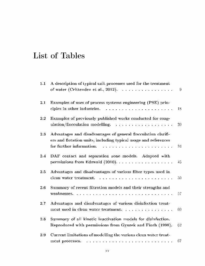
List of Tables
1.1 A description of typical unit processes used for the treatment
of water (Crittenden et al., 2012). . . . . . . . . . . . . . . . . 9
2.1 Examples of uses of process systems engineering (PSE) prin-
ciples in other industries. . . . . . . . . . . . . . . . . . . . . . 18
2.2 Examples of previously published works conducted for coag-
ulation/�occulation modelling. . . . . . . . . . . . . . . . . . . 30
2.3 Advantages and disadvantages of general �occulation clari�-
ers and �otation units, including typical usage and references
for further information. . . . . . . . . . . . . . . . . . . . . . . 34
2.4 DAF contact and separation zone models. Adapted with
permissions from Edzwald (2010). . . . . . . . . . . . . . . . . . 45
2.5 Advantages and disadvantages of various �lter types used in
clean water treatment. . . . . . . . . . . . . . . . . . . . . . . . 50
2.6 Summary of recent �ltration models and their strengths and
weaknesses. . . . . . . . . . . . . . . . . . . . . . . . . . . . . . . 57
2.7 Advantages and disadvantages of various disinfection treat-
ment used in clean water treatment. . . . . . . . . . . . . . . . 60
2.8 Summary of all kinetic inactivation models for disinfection.
Reproduced with permissions from Gyurek and Finch (1998). 62
2.9 Current limitations of modelling the various clean water treat-
ment processes. . . . . . . . . . . . . . . . . . . . . . . . . . . . 67
xv

LIST OF TABLES xvi
3.1 Model parameters for coagulation and �occulation model ver-
i�cation (Argaman, 1971). . . . . . . . . . . . . . . . . . . . . . 81
3.2 Actual and predicted performance of a multi-compartment
�occulator (Argaman, 1971). . . . . . . . . . . . . . . . . . . . . 81
3.3 Parameters to be implemented into gPROMS for the clari�-
cation unit (Burger et al., 2012). . . . . . . . . . . . . . . . . . 90
3.4 Parameters to be implemented in gPROMS for the rapid
gravity �ltration unit (Han et al., 2008). . . . . . . . . . . . . . 103
4.1 Plant data for Scenarios 1 - 3 (initial suspended solids con-
centration for Scenarios 1 and 2 is 6 mg/L and for Scenario
3 the initial suspended solids concentration is 4500 mg/L). . 115
4.2 Computational statistics of clean water treatment Scenarios
1 - 3. . . . . . . . . . . . . . . . . . . . . . . . . . . . . . . . . . 129
5.1 Desirability curve ranges presented for coagulation/�occulation
via rapid mixing as normalised and normal units of measure-
ment for Equations 5.3.2 and 5.3.3, along with justi�cations
for the ranges considered. . . . . . . . . . . . . . . . . . . . . . 139
5.2 Surrogate model β parameters for coagulation/�occulation
via rapid mixing. . . . . . . . . . . . . . . . . . . . . . . . . . . 139
5.3 Desirability curve ranges for coagulation/�occulation via �oc-
culation chambers/compartments presented as input units
of measurement for Equations 5.3.7 to 5.3.10, along with
justi�cations for the ranges considered. . . . . . . . . . . . . . 142
5.4 Surrogate model β parameters for coagulation/�occulation
via �occulation chambers/compartments. . . . . . . . . . . . . 142
5.5 Veri�cation of e�uent suspended solids concentration derived
from "logged" and "unlogged" surrogate model for coagula-
tion/�occulation via rapid mixing against the detailed model.
. . . . . . . . . . . . . . . . . . . . . . . . . . . . . . . . . . . . . 146

LIST OF TABLES xvii
5.6 Veri�cation of e�uent suspended solids concentration derived
from "logged" and "unlogged" surrogate model for �occula-
tion via �occulation in chambers/compartments against the
detailed model. . . . . . . . . . . . . . . . . . . . . . . . . . . . 147
5.7 Desirability curve ranges for clari�cation presented as coded
and uncoded units of measurement for equations 5.4.2 to
5.4.4, along with justi�cations for the ranges considered. . . 152
5.8 Surrogate model β parameters for e�uent suspended solids
concentration in clari�cation via sedimentation. . . . . . . . . 152
5.9 Surrogate model β parameters for under�ow suspended solids
concentration in clari�cation via sedimentation. . . . . . . . . 154
5.10 Veri�cation of e�uent suspended solids concentration derived
from "logged" and "unlogged" surrogate model for clari�ca-
tion via sedimentation against the detailed model. . . . . . . 159
5.11 Veri�cation of under�ow suspended solids concentration de-
rived from "logged" and "unlogged" surrogate model for clar-
i�cation via sedimentation against the detailed model. . . . . 160
5.12 Desirability curve ranges for �ltration presented as coded and
uncoded units of measurement for equations 5.5.2 to 5.5.4,
along with justi�cations for the ranges considered. . . . . . . 163
5.13 β parameters that have been determined to be utilised in
the surrogate model equation for e�uent concentration in
�ltration. . . . . . . . . . . . . . . . . . . . . . . . . . . . . . . . 163
5.14 Veri�cation of e�uent suspended solids concentration derived
from "logged" and "unlogged" surrogate model for �ltration
via rapid gravity �ltration against detailed models. . . . . . . 167
5.15 Assumptions and comments for the disinfection model devel-
opment. . . . . . . . . . . . . . . . . . . . . . . . . . . . . . . . . 169
5.16 Parameters ranges for disinfection units considered. . . . . . . 172

LIST OF TABLES xviii
5.17 Values used for disinfection model development in the inacti-
vation of Giardia for 3-log inactivation (99.9%) (Environmen-
tal Protection Agency, 2003a). . . . . . . . . . . . . . . . . . . . 172
5.18 Model test results in the prediction of e�uent microorganism
concentration from Equations 5.6.9, 5.6.10, and 5.6.11 for
inactivation of Giardia via disinfection using chlorine dioxide,
ozone and ultraviolet light. . . . . . . . . . . . . . . . . . . . . 175
5.19 Values used for disinfection model development in the in-
activation of Cryptosporidium for 2-log inactivation (99%)
(Environmental Protection Agency, 2003b). . . . . . . . . . . . 177
5.20 Model test results in the prediction of e�uent microorganism
concentration from Equations 5.6.12, 5.6.13 and 5.6.14 for in-
activation of Cryptosporidium via disinfection using chlorine
dioxide, ozone and ultraviolet light. . . . . . . . . . . . . . . . 178
A.1 Microbiological parameters (Directive, 1998) . . . . . . . . . . 219
A.2 Chemical parameters (Drinking Water Inspectorate, 2010) . . 220
A.3 Indicator parameters (Directive, 1998) . . . . . . . . . . . . . . 221
B.1 Reported kinetic parameters for �occulation kinetics Critten-
den et al. (2012) . . . . . . . . . . . . . . . . . . . . . . . . . . . 223
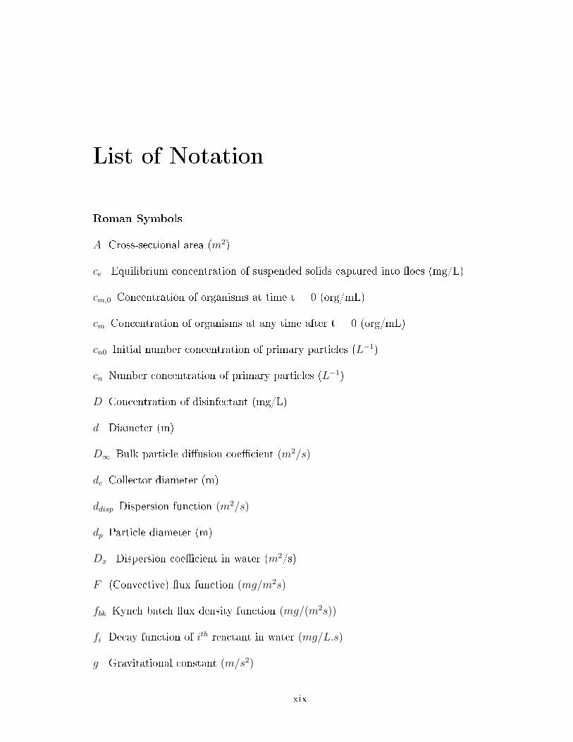
List of Notation
Roman Symbols
A Cross-sectional area (m2)
ce Equilibrium concentration of suspended solids captured into �ocs (mg/L)
cm,0 Concentration of organisms at time t = 0 (org/mL)
cm Concentration of organisms at any time after t = 0 (org/mL)
cn0 Initial number concentration of primary particles (L−1)
cn Number concentration of primary particles (L−1)
D Concentration of disinfectant (mg/L)
d Diameter (m)
D∞ Bulk particle di�usion coe�cient (m2/s)
dc Collector diameter (m)
ddisp Dispersion function (m2/s)
dp Particle diameter (m)
Dx Dispersion coe�cient in water (m2/s)
F (Convective) �ux function (mg/m2s)
fbk Kynch batch �ux density function (mg/(m2s))
fi Decay function of ith reactant in water (mg/L.s)
g Gravitational constant (m/s2)
xix

LIST OF NOTATION xx
G Velocity gradient (s−1)
I Intensity of UV radiation (W/cm2)
J Hydraulic gradient in the clogged �lter bed (-)
k Rate constant (s−1)
k1 Reaction rate (mg/L)1−γs−1)
KA Collision constant (-)
KB Break-up constant (s)
kc Kinetic constant, coe�cient of speci�c lethality for chlorine dioxide (L/mg.s)
ko Kinetic constant, coe�cient of speci�c lethality for ozone (L/mg.s)
kUV Kinetic constant, a function of transmittance (cm2/W )
N Number of deposited particles per �lter grain which acts as additional collectors
n Number concentration of particle (L−1)
N0 Inital particle count at time t=0 (-)
Nc Number of collectors in �lter grains (-)
Nt Total particle count at time t (-)
Q Volumetric �ow rate (L/s)
r Parameter in equation for fbk (L/mg)
T Absolute temperature (K)
u Super�cial �uid velocity (m/s)
V Volume (L)
v0 Settling velocity of a single particle in unbounded �uid (m/s)
vhs Settling velocity of a single particle in unbounded �uid (m/s)
w Maximum number of size categories in Smouluchowski equation (-)
xi Normalised input variables in�uencing predicted response Z for surrogate model (-)

LIST OF NOTATION xxi
xj Normalised input variables in�uencing predicted response Z for surrogate model (-)
Yi Current input variables in�uencing predicted normalised x for surrogate model (-)
Z Predicted response for surrogate model (-)
Dimensionless
NG Dimensionless gravitational force number given by (ρp−ρ)gd2p/18µu
NLO Dimensionless van der Waals number given by 4A/9πµd2pu
NR Dimensionless ratio of particle to collector size given by dp/dc
Greek Symbols
α Particle/�lter attachment coe�cients (-)
αp Particle/particle attachment coe�cients (-)
β Inverse of compactness factor (-)
β0 Constant co�cient for surrogate model (-)
βii Quadratic interaction coe�cient for surrogate model (-)
βij Quadratic interaction coe�cient for surrogate model (-)
βi Linear interaction coe�cient for surrogate model (-)
η Single collector removal e�ciency (-)
η0 Single collector contact e�ciency in the clean �lter bed (-)
ηp Single deposited particle contact e�ciency (-)
γ Empirical parameter which is related to the �ow rate (-)
λ Filtration equation coe�cient (-)
φ Coe�cient related to �oc resistance (-)
ρp Suspended solid density (mg/L)
σ Speci�c deposit (mg/L)
σc Critical speci�c deposit (mg/L)

LIST OF NOTATION xxii
τ Contact time (s−1)
τ Residence time (s)
Υ Order of reaction (-)
ε Filter medium porosity (-)
$ Detachment coe�cient (s−1)
$0 Constant for a particular �ltration system (s−1)
Subscripts
z Depth in the z-axis
c Concentration
e E�uent
f Feed
i Particles
j Particles
k Particles
n0 Concentrations of primary particles at time t=0 (mg/L)
ni ith and mth number of �occulation chambers
nm mth number of �occulation chambers
s Suspended solid
u Under�ow
Abbreviations
ANN Arti�cal Neutral Network
Bottom Depth of thickening zone (m)
CFD Computational Fluid Dynamics
DAEs Di�erential Algebraic Equations

LIST OF NOTATION xxiii
DAF Dissolved Air Flotation
NOM Natural Organic Matter
ODEs Ordinary Di�erential Equations
PBT Population Balance Theory
PDEs Partial Di�erential Equations
PSE Process Systems Engineering
RSM Response Surface Modelling
SCC Single Collector Collision
SST Secondary Settling Tank
TOC Total Organic Carbon
Top Height of clari�cation zone (m)
UV Ultraviolet
WTW Water Treatment Work
WWT Wastewater Treatment

Chapter 1
General introduction
In this chapter, a general background of water quality and raw water sources
are presented, along with a summary of the various processing units available
in normal clean water treatment facilities. The motivation and objectives of
this thesis are highlighted, followed by an outline of the thesis structure.
1.1 Scope
The availability of a reliable and clean supply of water is vital for our health and
well-being, and for agriculture, �sheries, industry and transportation. A major chal-
lenge facing a sustainable global future is the ever increasing demand for clean water of
adequate quality and quantity. Even though water is one of the world's most abundant
resources, there are many regions that are in low supply of clean water (Veoila, 2014).
A source of water that is deemed safe to drink or to use for preparation of food is
known as clean water or drinking water. Figure 1.1 shows the globally available raw
water that can be utilised as clean water sources. The �gure highlights that most of the
world's water is in the oceans and saline lakes; this water will be salty and will require
desalination in order to make it usable for most purposes. Fresh water is approximately
3% of the planet's water, but most of that is in the form of snow or ice. A report by
the United Nations warns that �overcoming the crisis in water is one of the greatest
human development challenges of the early 21st century� (UNDP, 2006). In 2008, 6.74
1

CHAPTER 1. GENERAL INTRODUCTION 2
Figure 1.1: Breakdown of the water availability in the world.
billion people (about 85% of the global population) had access to a piped water supply
through house connections, or to an improved water source through other means than
via a house connection (DEFRA, 2014). Generally, the main challenges currently facing
the water industry are (DEFRA, 2014):
� Population increase: The constant growth in global population leads to an increase
in the demand for water.
� Climate change: Warmer climates, extreme weather events, and an unexpected
increase in droughts can occur as a result of climate change. This decrease in water
availability will lead to poorer water quality and develop a threat in sustaining
economically important wildlife and species. With an expected decline in both
leakage and the demand from individual households, the overall water demand is
predicted to decrease; climate change will have an impact on the overall demand
as more water is utilised in hotter conditions. Also, the push for a low carbon
economy may increase water usage by industry.
In the UK, the problem of ensuring su�cient water supply that meets the stringent wa-
ter regulations, will be intensi�ed in the future by a combination of a rising population,
climate change and the increased di�culty of building major new water infrastructure
due to limitations in the amount of land accessible for new developments. Since the
1950s, household water demand has been increasing, due to changes in the use of water
in the home and population growth; it is now more than half of all public water supply
use, as shown in Figure 1.2 (DEFRA, 2014). It is estimated that the average water use
in England is currently about 150 litres per person per day, equivalent to approximately
one tonne of water per week.

CHAPTER 1. GENERAL INTRODUCTION 3
Figure 1.2: Public water supply for England and Wales (megalitres per day) (DEFRA,2014).
Within the EU, comparisons between country water usage are not always straightfor-
ward, although it seems many other countries are using signi�cantly less than England
(Figure 1.3). These current levels of water usage are unsustainable and recent e�orts
to address this usage have led to the development of new puri�cation processes and
improved water management techniques; however, over the next 20 years, behavioural
changes and technological innovation will be needed to �nd a balance between the
supply and demand of water (IChemE, 2007). One change currently being explored
is the use of advanced computational tools in the management of technological risk,
for example, arising from process uncertainty, innovation and early design decisions.
Innovation is essential for any business to establish and maintain a competitive advant-
age, and involves making decisions in the absence of complete information, and this
inevitably leads to risks. Computational tools, in this instance, can involve the use
of mathematical models for: (a) the e�ective quanti�cation of the technological risks
associated with model-based decisions and (b) the optimisation of process design and
operation through comprehensive studies into the alternatives. With successful imple-
mentation, tools will be able to predict the e�ects of design and operating decisions on
key performance indicators within the accuracy necessary to achieve business objectives.
Within the water industry, utilising computational tools will support decisions that
account for both the treatment process and the impact of these decisions on the other
parts of the business.

CHAPTER 1. GENERAL INTRODUCTION 4
Figure 1.3: EU per capita water consumption (DEFRA, 2014).
1.2 Water Industry: raw water
Water quality regulations
The European Directive (Directive, 1998) on the quality of water intended for human
consumption prescribes standards for the quality of drinking water, water o�ered for
sale in bottles or containers, and water for use in food production undertakings. The
requirements have been incorporated into the Water Supply Regulations 2000 in Eng-
land and Wales (Directive, 1998). The main objective of the water quality standards
is to protect human health from adverse e�ects resulting from excessive concentrations
of potentially health-damaging substances in drinking water. The presence of micro-
biological and chemical contaminants in drinking water can lead to acute or chronic
health e�ects, making the removal of these a primary concern for water treatment.
The directive distinguishes between di�erent contaminants by dividing them into two
types: mandatory (these cannot exceed a speci�c parameter value) and non-mandatory
(the speci�c parameter value can be used as an indicator) (Binnie and Kimber, 2009).
The mandatory standards covers 28 microbiological and chemical parameters that
are essential to be removed, whilst the non-mandatory standards covers 20 further
microbiological, chemical and physical parameters that are prescribed for monitoring
purposes (a table with all the parameters can be found in Appendix A). Microbes are

CHAPTER 1. GENERAL INTRODUCTION 5
the primary contaminants of concern particularly Giardia1 and Cryptosporidium2, as
they have adverse e�ects on our health. A speci�c regulation on the treatment of both
Giardia and Cryptosporidium has been set to less than one oocyst3, which are about
�ve thousandths of a millimetre in diameter - is less than one-tenth the thickness of
a human hair (Centers for Disease Control and Prevention, 2015a,b). The physical
parameters include indicators such as turbidity4, which is an important measure of
discoloured water. Turbidity is often used as the main indication for the presence of
suspended solids in the water (and will be discussed in more detail later).
1.2.1 Raw water sources
The type of raw water entering a clean water treatment plant will have an impact on
the degree of removal e�ciency for suspended solids throughout the system. Rational
selection of raw water sources requires a review of the alternative sources available
and their respective characteristics. The raw water that is used for drinking water
treatment plants are categorised based on their source as upland water, lowland water,
and a mixture of water that can be held in a reservoir. Upland water (surface water) can
be from moorland springs and rivers, which have higher suspended solids concentration
due to the fact they have contact with mineral deposits in the soil. Lowland waters
(groundwater) are fed from upland lakes and groundwater springs and these have a lower
suspended solids concentration as these waters are found in underground aquifers. This
means many of the microorganisms and suspended solids have to pass through solids
and rocks which act as a �lter. The organic content of these waters can vary signi�cantly
from season to season especially following the �rst winter rains.
Groundwater
Any water that is underground can be classi�ed as groundwater. Although groundwater
is generally considered to be less likely to be contaminated than surface water, it may
still require contaminant removal. Some surface water sinks into the ground, passing
1Giardia is a microscopic parasite that is considered one of the most common sources of waterborneillnesses (Centers for Disease Control and Prevention, 2015b). It is an intestinal infection identi�ed byabdominal cramps, bloating, nausea and periods of watery diarrhoea.
2Cryptosporidium is a protozoan parasite that can infect the gut, thus causing an infection whichleads to diarrhoea (Centers for Disease Control and Prevention, 2015a).
3An egg-like state of microscopic parasites that can be found in clean water (Centers for DiseaseControl and Prevention, 2015a).
4Turbidity is a key measurement of water quality and can be de�ned as the cloudiness in the �uidcaused by suspended solids that are generally invisible to the naked eye (Binnie and Kimber, 2009).

CHAPTER 1. GENERAL INTRODUCTION 6
Figure 1.4: Illustration to show how water enters the unsaturated zone (soil moisture)and the saturated zone (groundwater) (Environment and Climate Change Canada,2013).
through layers of sand, clay, rock, and gravel which clean the water (as can be seen
in Figure 1.4). The water that sinks into the groundwater occurs in two di�erent
zones: unsaturated zone and saturated zone. In the unsaturated zone, pore spaces
contain air; therefore, groundwater can not be easily taken from this zone. Usable
groundwater occurs in the saturated zone, where pore spaces are completely �lled with
water. Even though groundwater will not be exposed to the same contaminants that
surface water is subjected to, contaminants can nevertheless still be introduced; for
instance, by rain washing fertilisers and insecticides into the soil where they will sink into
the groundwater. The groundwater zones are contained and situated within aquifers
and springs.
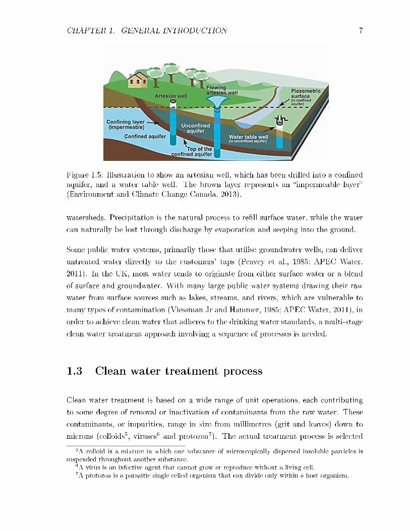
Aquifers can be classi�ed by two types: con�ned and uncon�ned. Con�ned aquifers may
be shallow or deep (Binnie and Kimber, 2009), and are characterised by being separated
from the surface by an impermeable layer that con�nes the groundwater above and
below it (Figure 1.5). An uncon�ned aquifer is often shallow, and it primarily contains
permeable material. The top of the aquifer is called the water table although it does
not have a �at surface, but has high areas and low areas.
Surface Water
Surface water is classi�ed as water that collects on the ground or in streams, rivers,
lakes or wetlands. The majority of these waters are exposed to contaminants due
to the water being open to the atmosphere. Common contaminant sources can stem
from untreated sewage and runo� from fertilised �elds, parking lots, or unprotected
CHAPTER 1. GENERAL INTRODUCTION 7
Figure 1.5: Illustration to show an artesian well, which has been drilled into a con�nedaquifer, and a water table well. The brown layer represents an �impermeable layer�(Environment and Climate Change Canada, 2013).
watersheds. Precipitation is the natural process to re�ll surface water, while the water
can naturally be lost through discharge by evaporation and seeping into the ground.
Some public water systems, primarily those that utilise groundwater wells, can deliver
untreated water directly to the customers' taps (Peavey et al., 1985; APEC Water,
2011). In the UK, most water tends to originate from either surface water or a blend
of surface and groundwater. With many large public water systems drawing their raw
water from surface sources such as lakes, streams, and rivers, which are vulnerable to
many types of contamination (Viessman Jr and Hammer, 1985; APEC Water, 2011), in
order to achieve clean water that adheres to the drinking water standards, a multi-stage
clean water treatment approach involving a sequence of processes is needed.
1.3 Clean water treatment process
Clean water treatment is based on a wide range of unit operations, each contributing
to some degree of removal or inactivation of contaminants from the raw water. These
contaminants, or impurities, range in size from millimetres (grit and leaves) down to
microns (colloids5, viruses6 and protozoa7). The actual treatment process is selected
5A colloid is a mixture in which one substance of microscopically dispersed insoluble particles issuspended throughout another substance.
6A virus is an infective agent that cannot grow or reproduce without a living cell.7A protozoa is a parasitic single-celled organism that can divide only within a host organism.

CHAPTER 1. GENERAL INTRODUCTION 8
Figure 1.6: Main technologies available for water treatment processes.
based on various factors; the most critical being the nature of the water source and the
intended use of the treated water.
There are a variety of unit operations that can be utilised for clean water treatment,
which may vary slightly depending on di�erent locations, the technology of the plant
and the water it needs to process; however, the basic principles are largely the same.
Figure 1.6 shows the hierarchical organisation of a typical water treatment work, where
each main process (e.g. coagulation/�occulation) can have a variety of unit operations
that can be selected to ful�l the requirements of that process (rapid mixing or �occu-
lators). Table 1.1 explains in more detail the various unit operations and their typical
applications.
Water treatment can be classi�ed into clean water and wastewater treatment. The
main di�erence between the two types of water treatment are the sources of water.
For clean water treatment plants, generally the type of water that comes in is taken
from surface water, groundwater or rainwater which is cleaned and distributed for
human consumption; however, wastewater treatment plants collect sewerage and other
wastewaters from various sites (such as from houses, industry etc.), cleans it and releases
it back to the environment at a safe level for humans, �sh and plants to be around. For
these two types of treatment, the units can be broadly categorised into chemical and

CHAPTER 1. GENERAL INTRODUCTION 9
Table 1.1: A description of typical unit processes used for the treatment of water(Crittenden et al., 2012).
Process Unit
operations
Description Typical Application in
Water treatment
Coagulation Rapid
Mixing
Process of destabilising colloidalparticles so that particle growthcan occur during �occulation.
Mixing and blending two ormore soluble solutions throughinput of energy.
Addition of chemicals (solublesolutions) such as ferricchloride, alum, and polymers todestabilise particles found inwater.
Flocculation Flocculator Aggregation of particles that
have been chemically
destabilised through
coagulation.
Used to create larger particlesthat can subsequently be morereadily removed by otherprocesses such as gravitysettling or �ltration.
Clari�cation Clari�er Removal of solids by gravity
settling.
Used to remove particles greaterthan 0.5 mm in diameter,generally following coagulationand �occulation.
Flotation Removal of �ne particles and�occulated particles withspeci�c gravity less than wateror with very low settlingvelocities so they �oat to thetop of the �uid.
Removal of particles following
coagulation and �occulation for
high quality raw waters that are
low in turbidity, colour and/or
total organic carbon.
Filtration Traditional
(Rapid
gravity)
The removal of particles bypassing water through a bed ofgranular material; particles areremoved by transport andattachment to the �lter media.
Removal of solids following
coagulation and �occulation,
gravity sedimentation or
�otation.
Membrane The removal of particles bypassing water through a porousmembrane material; particlesare removed by size exclusionbecause the particles are largerthan the pores.
Used to remove colour
(turbidity), viruses, bacteria,
and protozoa such as Gardia
and Cryptosporidium.
Disinfection Chemical
disinfection
Addition of oxidising chemicalagents to inactivate pathogenicorganisms in water.
Disinfection of water withchlorine, chlorine compounds, orozone.
UV light
oxidation
Use of UV light to oxidisecomplex organic molecules andcompounds by disrupting theDNA structure ofmicroorganisms.
Used for oxidation of organic
molecules, such as in bacteria.

CHAPTER 1. GENERAL INTRODUCTION 10
physical processing units. In chemical units, a chemical is added to induce a response;
for instance, chlorine is added to inactivate bacterial microorganisms in the disinfection
stage. The unit operations in physical processing units cause a physical change to the
treated water; for instance, the impeller in the �occulation unit promotes growth of
small colloidal particles after the addition of a chemical additive.
The raw water feed into clean water treatment processes often contain colloidal particles
that cause the water to appear cloudy. The raw water is initially passed through
mechanical mesh screens to remove large debris, after which it enters the coagulation
unit. Chemical coagulants, such as aluminium sulphate, are then added to the raw water
to destabilise the colloidal particles and this encourages the rapid formation of small
particles, or agglomerates, through �occulation8. Solid-water separation processes, such
as sedimentation, are used to reduce the �oc concentration in the treated water; these
unit types are broadly called clari�cation units, and they are important as they ensure
the subsequent treatment process (usually �ltration) can be operated more easily and
cost-e�ectively to produce quality water. The process of �ltration consists of passing
water through a porous medium such as a bed of anthracite sand or other suitable
material to retain solid matter whilst allowing the water to pass through. In order to
achieve the required quality of �ltered water, the �ltration system has to retain particles
larger than the pores and allow a �ow of water to pass through the bed of media at a
low speed. This will ensure the media retains most solid matter while permitting the
water to pass to a �nal disinfection stage. The disinfection units are used to target the
removal of microorganisms through the use of chemicals such as chlorine, UV dosing
and ozonation.
1.4 Motivation
With a growing population and the impact of climate change, as well as reduced space
available for new infrastructure, there are increasing pressures on the water industry.
There is a greater need for more e�cient water treatment works, whether it is to
increase throughput, minimise capital expenditure or reduce operational costs. A better
understanding of the fundamental knowledge of the individual treatment units and
their interactions, including an understanding of the dynamic behaviour of the works,
is needed in order to mitigate risks, such as reduced levels of water purity in distribution
8Flocculation is the promotion of �oc growth through collision either in a slow mixing unit or usingmovement through ba�ed chambers.

CHAPTER 1. GENERAL INTRODUCTION 11
due to an unexpected change in the earlier treatment processing steps. Although
drinking water treatment works have been functioning for more than a century, in the
last few decades the operation has become more and more complex (Trussell, 2000),
which makes e�cient management more challenging.
The operation of drinking water treatment works has traditionally been based on
experience. Current raw water quality and �ow can be di�erent from what the treat-
ment processes were originally designed to handle. Due to more stringent regulations
(DEFRA, 2009), plants have to produce water of an increasingly higher quality, which
requires intensive quality monitoring of the source, the product, and of the treatment
work operation. Raw water quality is subject to changes, and these can be seasonal
e�ects (e.g. temperature, turbidity), which a�ect long-term trends (e.g. salt content)
or short-term trends (e.g. sudden heavy rain fall). The management of a treatment
work can therefore be challenging, but the works are not currently controlled to the
same level as, for instance, a chemical plant.
The IChemE technical strategy road-map (IChemE, 2007) indicates that technological
advances are needed to secure sustainable water supplies, and research priorities should
include water puri�cation, water treatment, and sewage sludge disposal. The techno-
logies utilised in water treatment can be energy intensive and the energy footprint in
water can be substantial. In the UK, approximately 3% of the total national electricity
consumption is utilised by the water industry. Over the past 20 years, the energy use
has increased signi�cantly, with power costs making up 13% of total production costs,
and only 10% of power originating from renewable sources (Rothausen and Conway,
2011).
The challenge of meeting water demands is a complex one, demanding a di�cult mix of
political intervention, new technology, improved water conservation and distribution,
increased technical and engineering skills. According to Rosen (2000) and Trussell
(2000), by 2050 a drinking water treatment work will be entirely controlled from a cent-
ral control centre, where dedicated integral control programmes incorporating advanced
process and control models will control the treatment processes and mitigate risk. The
development of detailed mathematical model representations of each water treatment
process is therefore essential in order to meet this objective. Mathematical models
are descriptions of real world systems, which can help enhance the understanding of
the behaviour of complex systems. Many industries, such as chemicals, pharmaceuticals
and food, are already making extensive use of mathematical modelling and optimisation
tools as a way of enhancing their processes (Barakat and Sørensen, 2008; Klatt and

CHAPTER 1. GENERAL INTRODUCTION 12
Marquardt, 2009; Bennamoun et al., 2009; Wang et al., 2013). Models used for these
purposes, and to simulate the operation of a drinking water treatment work, must be
accurate and must capture the main behaviour of the process, but must also be valid
under changing process conditions.
Currently, research available in literature tends to narrow its focus to modelling speci�c
aspects of each processing unit as opposed to focusing on the treatment work as a
whole. For example, the mechanism for the removal of colloidal particles suspended in
water has been extensively researched and modelled for the coagulation, �occulation
and sedimentation unit operations individually (Holtho� et al., 1996; Edzwald and
Van Benschoten, 1990; Edzwald, 1993; Saritha et al., 2015) but not how their interac-
tions can be e�ectively utilised. A plant-wide modelling approach will allow for e�ective
risk mitigation as the ability to see the cause and e�ect of changes through simulation is
a powerful tool. Within the water industry, most modelling work tends to be empirical9
rather than mechanistic10. The empirical approach is not rigorous and use of such mod-
els is limited to only speci�c applications and conditions, which is time consuming when
trying to create varying scenarios. Mechanistic models are more robust and develop
a more detailed understanding of the fundamentals occurring within unit operations.
There are some existing models that are heavily reliant on mechanistic models based
on experimental data. Many �occulation `models' are data-driven (Thomas et al.,
1999; Heddam et al., 2012) and are therefore di�cult to generalise or extend to other
treatment works. Other treatment processes, such clari�cation and �ltration, have been
more widely studied and the models incorporate more phenomenological occurrences
so the models are on a sounder basis. A mathematical model that can provide a
description of the connections between the individual units will be an important step
in the direction of controlling a water treatment work via a central control centre.
In a process systems engineering approach, mathematical models are mainly derived
from �rst principles utilising fundamental knowledge of the phenomena occurring.
These models can, however, be quite complex, and simpler �surrogate� models can be
derived from these models which will still be able to predict trends but at a fraction of
the computational power. A system based on surrogate models would be an advantage
(in comparison to a time consuming detailed model) to a central control centre, leading
to monitoring of the water treatment works in real time. As the water industry aims
9Empirical modelling is based on empirical observations rather than on mathematically describablerelaitonships of the system modelled.
10Mechanistic modelling is based on fundamental chemical and physical relationships which can bemathematically described, such as, di�usion.

CHAPTER 1. GENERAL INTRODUCTION 13
to gain a competitive advantage, the implementation of a simpler surrogate model as
an optimisation tool utilising fundamental knowledge would be bene�cial as it can be
applied to any site, with a change in the conditions.
1.5 Objectives and contributions of this thesis
Current research in the area of modelling clean water treatment works is young when
considering the long history of the water treatment industry. As stated earlier, funda-
mental research so far has mainly focused on gaining an understanding of the individual
units. To the best of the author's knowledge, currently no full mathematical model
based on �rst principles which describes an entire conventional clean water treatment
work is available in the open literature. The primary aim of this thesis is therefore to
draw upon previous work in the literature to develop a �rst principles mathematical
model of an entire conventional clean water treatment work.
The main deliverables from this work are:
1. A critical assessment of the current state-of-art in mathematical modelling in the
clean water treatment industry, focusing on detailed mathematical models and
optimisation techniques.
2. Development and validation of mathematical models for each of the main unit
operation in a conventional clean water treatment works.
3. Development of a complete mathematical model of conventional clean water treat-
ment works that can accurately describe the water treatment process mechanisms,
and the connections between individual units.
4. Development of surrogate models for incorporation into a systematic method for
the synthesis of clean water treatment works. These surrogate models should be
able to accurately predict the mechanistic trends of the corresponding detailed
mathematical model.
1.6 Organisation of this thesis
An introduction to the relevance of developing mathematical models of clean water
treatment processing units has been given, and the general aim of the work has been set

CHAPTER 1. GENERAL INTRODUCTION 14
out. The rest of the thesis is divided into six chapters. Chapter 2 provides an extensive
literature review of current work related to modelling of processing units utilised in
the water industry. An overview of the di�erent methods, models and techniques
currently available are analysed to comprehensively evaluate the applicability of these
mathematical modelling tools.
Chapter 3 examines the development of mathematical models of clean water treatment
unit operations based on �rst principles followed by model validation based on data
from literature. The mathematical models considered are the three physical processing
units in the conventional clean water treatment process: coagulation/�occulation, cla-
ri�cation and �ltration. This chapter highlights that the knowledge and understanding
of the individual clean water processing units can be advantageous through varying
case studies and will lead to robust complete water treatment work models.
Chapter 4 considers the development and application of a complete water treatment
work model. A �rst principles modelling based approach for linking individual clean
water processing units, which are commonly studied in isolation, is proposed. Use of
the model can include process development for design purposes, or as a training tool
for work operators. The main advantages in the use of modelling can be realised when
computational tools can be used as risk mitigation by simulating feedback responses to
proposed changes in the work.
Chapter 5 addresses the need for computationally e�cient mathematical models within
the water industry, and explores the use of surrogate modelling techniques for optim-
isation or control purposes. The use of complex mathematical models will result in
excessively detailed treatment work models and this could prove di�cult to validate
with a real world clean water treatment works. In addition to this, operators will
need to be trained in order interact with the advanced computational tools used for
detailed modelling whilst the simpler surrogate models can be simulated on Microsoft
Excel which is more user friendly. The use of surrogate models will also reduce the
computational time demand and this is an advantage in an industry that is trying to
move away from, reactive to proactive approaches in its operation.
Finally, Chapter 6 concludes with the major �ndings of this work and with conclusions
from each part of the project. A number of areas for future work are discussed. The
chapter focuses in particular on the broader implications for the use of fundamental
models of processing units in the water industry.

Chapter 2
Literature review
This chapter is divided into sections which present a detailed literature
review on various processes in clean water treatment that motivate the objec-
tives of this work, as outlined in chapter 1. The chapter begins by assessing
the current state-of-the-art surrounding the use of mathematical models in
the water industry, which is followed by how application of various methods
utilised by process systems engineering can prove propitious to the clean
water treatment processes.
2.1 Introduction
Water companies have resource management plans which look 25 years ahead to show
projections of future demand for water and how the companies aim to meet this demand
(Davies and Daykin, 2011). Every day, the UK water industry collects, treats and
supplies more than 17 billion litres of puri�ed water for domestic and commercial
use, whilst simultaneously collecting and treating over 16 billion litres of the resulting
wastewater to return to the environment (Binnie and Kimber, 2009).
To treat a particular water source, there are a number of key treatment processing
steps that are generally used, most commonly coagulation, �occulation, clari�cation,
�ltration and disinfection, and each main step has a number of variations. The actual
15

CHAPTER 2. LITERATURE REVIEW 16
treatment process route is selected based on various factors (Binnie and Kimber, 2009)
as stated earlier, the most critical being the nature of the water source and the intended
use of the treated water.
Traditionally, the water industry has been sitting within the civil engineering domain
rather than the chemical engineering domain; however, due to the increasing pressure
for companies to remain competitive in the national or global marketplace, the search
for e�cient methodologies for operational management and mitigation of risk has led
some to consider the use of Process Systems Engineering (PSE) methods, in particular,
detailed modelling from �rst principles, which have been highly successful within the
chemical industries. The use of PSE methods for design and control within water
treatment has been shown to lead to better water quality, cost reduction and to a
greater stability performance of the plant as well as to an increased understanding of
the individual treatment processing steps (Brouwer and De Blois, 2008; Rietveld et al.,
2009). Modelling of the individual steps in clean water treatment has received some
attention in terms of design and operation; however, very little has been considered in
terms of the integration of the individual steps to create a representation of the overall
plant performance which can be used for operational management.
The �rst part of this chapter will de�ne what is meant by Process Systems Engineering
(PSE) in a water treatment context, and will outline how this area has led to signi�cant
advances within other industries which are related, or similar, to clean water treatment
(Klatt and Marquardt, 2009; Stephanopoulos and Reklaitis, 2011; Gernaey et al., 2012).
At the core of any Process Systems Engineering (PSE) methodology is a detailed
mathematical model of the process under investigation, and the second part of this
chapter will focus on assessing the current state-of-the-art on the models available for
the di�erent clean water treatment processing steps, both as individual units and as a
complete plant. These models can be incorporated into a wider PSE approach within
clean water treatment with the aim to achieve better plant designs or retro�ts as well
as vastly improved operational management.
2.2 What is Process Systems Engineering (PSE)?
Process Systems Engineering (PSE) is an established area within chemical engineering
with roots dating back to between the 1950s (Klatt and Marquardt, 2009) and the
1960s (Grossmann and Westerberg, 2000), with its progression closely linked to the

CHAPTER 2. LITERATURE REVIEW 17
developments within computing. PSE involves the understanding and use of systematic
and model-based solutions for the design and operation of chemical process systems
(Ponton, 1995). There are numerous �elds of PSE that have been considered in the past,
are currently under investigation or are anticipated to be of high relevance to industry
in the future. Grossmann and Westerberg (2000) provided a condensed summary of
the main �elds within the headings of process and product design, process control,
process operation, and supporting tools. A few examples of how PSE methodologies
have been applied in other industries are given in Table 2.1 to illustrate typical usage
and advantages.
2.2.1 Fundamentals and methodologies of PSE
At the heart of any PSE method lays a mathematical model. A mathematical model
is a description of a system in terms of equations that has been formulated to describe
how the system behaves and to predict the physical and/or chemical behaviour of the
system under di�erent conditions. A simulation solves the equation set and shows
either the conditions of the system at steady state or how the system behaves over
time from a given initial condition (dynamic). The bene�t of the simulation depends
to a large extent on the accuracy of the model, i.e. whether the equations accurately
describing the process in terms of its physical and/or chemical behaviour, and whether
the parameter values used are accurate, i.e. statistically signi�cant.
There are two main approaches to developing mathematical models: empirical mod-
elling and mechanistic modelling. Empirical models are based on direct observation,
measurement and extensive data records. These models depend on the availability of
representative data for model building and validation with a �trial and error� approach
is often adopted. Mechanistic models are based on a fundamental understanding of the
chemistry and physics governing the behaviour of the system. They do not require much
data for model development beyond that required for determining model parameters.
The term �mechanistic model� is broad as it covers a variety of model types such as
sets of ordinary di�erential equations (ODEs), di�erential algebraic equations (DAEs),
and partial di�erential equations (PDEs).
Most modelling work within water operations has so far been based on empirical obser-
vations or hydraulic modelling1 rather than mathematically describable relationships
1A hydraulic model is a mathematical model of a �uid introduced into a water/wastewatersewer/storm sewer system at various rates and pressures. These models can be used to analyse systemhydraulic behaviour under variable conditions (Novak et al., 2010).

CHAPTER 2. LITERATURE REVIEW 18
Table 2.1: Examples of uses of process systems engineering (PSE) principles in otherindustries.
Industry Research area Numerical
techniques
Advantages Author(s)
Chemicals Heat exchanger
and distillation
network
synthesis.
One, two and threedimensional �niteelement, �nitedi�erence and �nitevolume methods.
Network optimisation
using linear and
non-linear
programming.
By optimising design andoperating conditions,more consistent andbetter product qualitycan be achieved.
Improves competitiveness
and increases pro�tability
of their core business.
(Klatt and
Marquardt,
2009;
Barakat and
Sørensen,
2008;
Kleme² and
Kravanja,
2013;
Ochoa-Estopier
et al., 2014)
Drying Direct drying
systems (i.e.
�ash dryers,
spray dryers.
etc).
Computational �uid
dynamics (CFD).
Better understanding anddesign of dryingequipment with less costand e�ort thanlaboratory testing.
Techniques have been
successfully adapted to
simulate the thermal
processes of industrial
dryers. These techniques
have been routinely used
owing to the availability
of user-friendly
commercial packages.
(Bennamoun
et al., 2009;
Jamaleddine
and Ray,
2010)
Food Heating and
cooling
processes
One, two and three
dimensional �nite
element, �nite
di�erence and �nite
volume methods.
Deeper understanding offood processing means itis possible to evaluatedesign alternativesquickly and startcommercial production ata faster rate.
Models have the potential
for integration with other
models, such as
biochemical and
microbial reactions.
(Wang et al.,
2013)

CHAPTER 2. LITERATURE REVIEW 19
Figure 2.1: Graphical representation of the modelling process. Adapted withpermissions from Sargent (2005).
of the process through mechanistic modelling. As mentioned earlier, the empirical
approach to modelling is not rigorous and use of such models is limited to the speci�c
conditions used in the development of the model. Mechanistic models, however, can be
used for other applications of a similar type, and to some extent under other conditions,
and are therefore far more powerful. For example, a mechanistic model developed for
a distillation column in a re�nery can be used to model a distillation column on other
process plants, subject to varying conditions.
Roger Sargent, widely accepted as the Father of PSE, introduced a paradigm that relates
model veri�cation and validation to the model development process as illustrated in
Figure 2.1 (Sargent, 2005). The real or proposed process to be modelled can be broadly
labelled as the �area of interest�. The �conceptual model� is used to narrow down the area
of interest to a speci�c study domain, e.g. an individual process unit, which will be the
focus of the mathematical representation. At this stage, the theories and assumptions
underlying the conceptual model are considered, checked and it is decided if the model
will be �t for purpose, e.g. are the right parts of the process considered and under the
right operating conditions. The representation is then implemented as a mathematical
equation set within a �computer model�. The validity of the computer model has to be
veri�ed. Here, veri�cation is de�ned as ensuring that both the equation set and the
implementation of the model are accurate. The operational validation determines if the
model's output has obtained a su�cient accuracy for the intended purpose, and this is

CHAPTER 2. LITERATURE REVIEW 20
done through a series of computational experiments or simulation runs, under di�erent
scenarios or conditions. At the centre of the modelling process lies data validity, which
is de�ned as ensuring that the necessary data for model building, validation and testing
are all adequate and accurate to the required degree of accuracy. This data is usually
obtained either from plant data or from separate experiments.
Modelling and simulation o�er an e�cient and powerful tool for system analysis which
is as applicable to the clean water industry as it is to the chemical industries. Although
the use of mathematical modelling is still limited within the clean water treatment
industry, the use of mathematical modelling within the wastewater treatment industry,
for instance, has become increasingly popular since its introduction in the mid-1990s
(Dupont and Sinkjaer, 1994). Simulations using veri�ed and accurate models can be
used to obtained valuable information about a process far quicker than experiments
and with minimal cost, and will lead to better water quality, reduction in capital
expenditure, and more stable performance of a plant due to the increased understanding
of the phenomena occurring.
2.2.2 Enterprise-wide optimisation
Enterprise wide modelling and optimisation is an area of research that lies in the
interface between chemical engineering and operations research (Grossmann, 2005).
There have been several papers that have reviewed enterprise-wide optimisation in terms
of supply chain management in addition to process modelling and control (Larsson and
Skogestad, 2000; Shah, 2005; Charpentier, 2005; Varma et al., 2007); however, as with
all emerging technologies, EWO has challenges it has to face before it can be fully
functional. One of the challenges highlighted by Grossmann (2005) states a major issue
is integration of novel mathematical programming to capture the complexity of the
various process operations.
One of the key features in the incorporation of a mathematical model of a full WTW
is the integration of information and decision making amongst functions that comprise
the process control region. According to Trussell (2000), Rosen (2000) and Grossmann
(2005), within the next 30 years, a clean water treatment plant will be controlled
from a central control centre where the dedicated integral control programmes which
incorporate advanced process and control models will control the entire process.
Figure 2.2 represents an integrated framework for the application of a PSE method
into the water industry. The collection of data in the water industry is by Supervisory
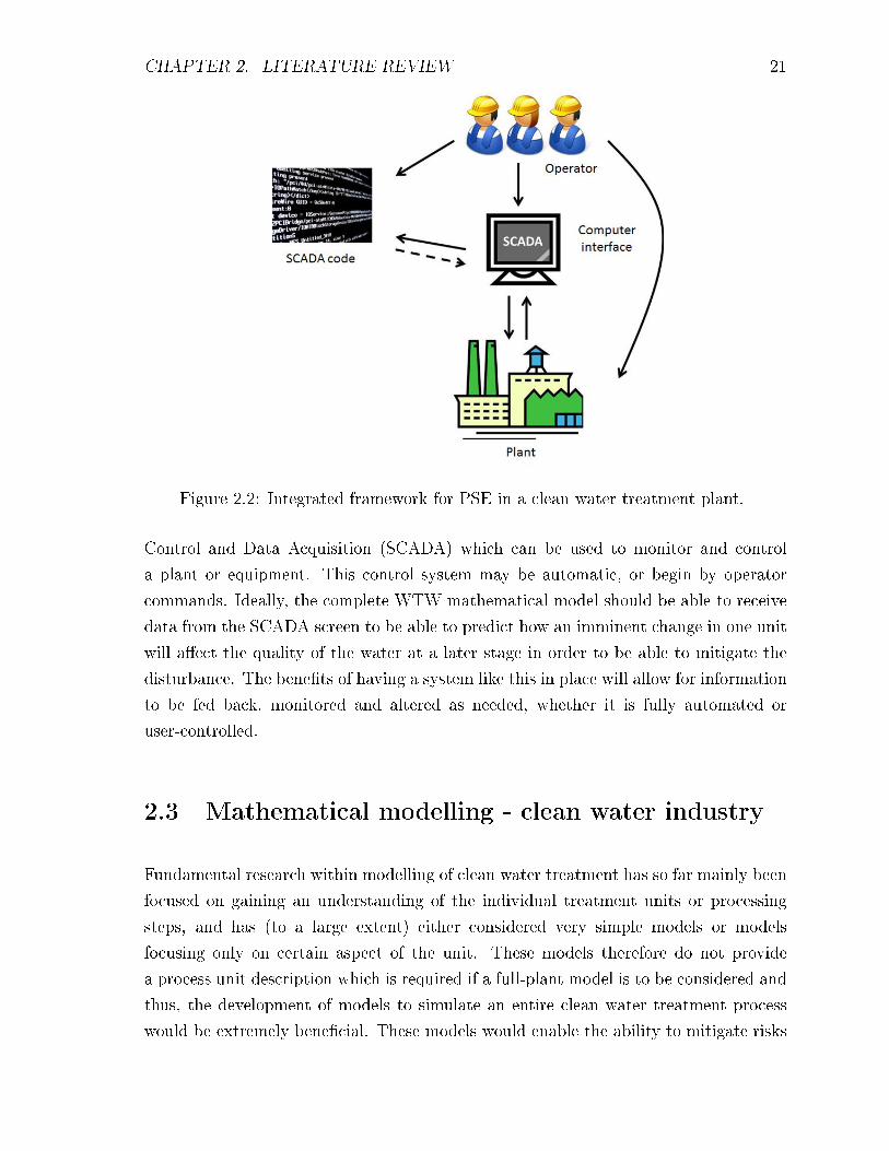
CHAPTER 2. LITERATURE REVIEW 21
Figure 2.2: Integrated framework for PSE in a clean water treatment plant.
Control and Data Acquisition (SCADA) which can be used to monitor and control
a plant or equipment. This control system may be automatic, or begin by operator
commands. Ideally, the complete WTW mathematical model should be able to receive
data from the SCADA screen to be able to predict how an imminent change in one unit
will a�ect the quality of the water at a later stage in order to be able to mitigate the
disturbance. The bene�ts of having a system like this in place will allow for information
to be fed back, monitored and altered as needed, whether it is fully automated or
user-controlled.
2.3 Mathematical modelling - clean water industry
Fundamental research within modelling of clean water treatment has so far mainly been
focused on gaining an understanding of the individual treatment units or processing
steps, and has (to a large extent) either considered very simple models or models
focusing only on certain aspect of the unit. These models therefore do not provide
a process unit description which is required if a full-plant model is to be considered and
thus, the development of models to simulate an entire clean water treatment process
would be extremely bene�cial. These models would enable the ability to mitigate risks

CHAPTER 2. LITERATURE REVIEW 22
Figure 2.3: Typical process diagram for clean water treatment plant (with examples ofvariations).
by simulating feedback responses to proposed changes in the work. Use of such models
can improve process development for design purposes, or as a training tool for work
operators.
The processing steps or units used in clean water treatment plants generally vary
depending on the source of raw water and the intended use of the treated water. In
addition, the performance of one treatment unit a�ects the performance of the later
units in the treatment process; hence, the evaluation of the performance of an overall
clean water treatment plant becomes a highly complex problem.
Figure 2.3 presents a general schematic of conventional treatment processes for clean
water, including examples of variations depending on the source water characteristics
for pre-treatment stages (which are pH adjustment controls and mechanical units,
such as, screens), coagulation (rapid mix), �occulation (contact tanks), clari�cation
(sedimentation, �oc blanket clari�ers, dissolved air �otation), �ltration (rapid gravity,
slow sand and membrane �ltration) and chemical disinfection (chlorine, chlorine dioxide,
chloramine, ozone and ultraviolet light). The physical process of each processing step
can be studied and modelled in a variety of ways, which will lead to the enhanced
fundamental knowledge; however, research tends to narrow its focus on speci�c aspects
for each unit. The rest of this chapter is divided as follows: sub-section 2.3.1 consid-
ers the current debate between a correlation between turbidity and suspended solids
concentration, which is an important consideration as suspended solids concentration
is the usual variable in the mechanistic mathematical models whilst turbidity is the
real world monitor for suspended solids concentration. Then sub-sections 2.3.2 to 2.3.5
review the available mathematical models for di�erent aspects within the coagulation
and �occulation, clari�cation, �ltration and disinfection treatment processes. These
sub-sections evaluate the available models focusing on comparisons and similarities

CHAPTER 2. LITERATURE REVIEW 23
between mathematical models available in the clean water industry and within the
water industry in general. Section 2.4 focuses on drawing from literature some answers
to common questions. For example, why fundamental knowledge is based on particle
concentration whilst real world application utilises turbidity, and whether a correlation
can be found? Based on knowledge of the background chemistry, how can this informa-
tion be incorporated to formulate process models? What are the current �ndings from
the use of models in wastewater treatment and can these be applied to the clean water
industry? Finally, Section 2.6 concludes with the major �ndings and conclusions from
each part of the sections.
2.3.1 Turbidity vs. Suspended solids concentration
Particles present in water, such as suspended solids and dissolved coloured material,
reduce water clarity by creating an opaque appearance. The number of particles and
their size distribution should be taken into account in order to accurately describe
the behaviour of the treatment process using a mathematical model. Turbidity is the
cloudiness of a �uid caused by a large number of particles, which individually are
invisible to the naked eye, and it is used as a measure by treatment plants of how
much suspended solids are present in the water. The turbidity of water is measured
based on the amount of light scattered by the suspended solid particles in the water
(Perlman, 2004). The more suspended solid particles present then more light will be
scattered. As such, turbidity can be related to the number of suspended solids particles
through particle concentration and particle size distribution, both strongly in�uencing
the scattering of the light (Kleizen et al., 1995). Turbidity is not a direct measurement
of the total suspended materials in the water, but instead serves as a measure of the
relative clarity of the water. Turbidity is often used to indicate changes in the total
suspended solids concentration in the water but without providing an exact measure of
the quantity of the suspended solids (Kemker, 2014).
Much research has been devoted to improving the understanding of turbidity in wa-
ter treatment processes (Edzwald and Van Benschoten, 1990; Thompson et al., 2003;
Hannouche et al., 2011), for example, it has been shown that for most surface waters,
coagulant doses should be determined by the concentration of natural organic matter
(NOM) rather than by turbidity (Edzwald and Van Benschoten, 1990), and this is a
practice that is still used today. There is still considerable work to be done in �nding
a predictive correlation between turbidity and particle concentration in order to use

CHAPTER 2. LITERATURE REVIEW 24
plant data based on turbidity in a mathematical model which considers a concentration
of suspended solids. It is often assumed that turbidity provides a direct measure
of suspended solids concentration and that there is a formula or set of conversion
factors with which suspended solids concentration can be calculated from Nephelometric
Turbidity Unit (NTUs). Hannouche et al. (2011) con�rm the existence of a strong
linear relationship between turbidity and suspended solids concentration; however,
their relationship has limitations depending on dry and wet weather conditions. It
can be concluded that a greater understanding of suspended solids suspensions and
their predictive relationship with turbidity is needed in order to adequately model and
verify with a clean water treatment plant.
2.3.2 Coagulation and �occulation
In a clean water treatment work, water from reservoirs and rivers containing colloidal
and small particles of algae, grit and gravel pass through a preliminary treatment stage
consisting of screens to physically remove the larger solids, and other debris before
the water passes to the main treatment process. The �rst main step of the clean
water treatment process is usually coagulation and �occulation. This step is in fact a
three stage process, consisting of rapid mixing, coagulation of colloidal particles and
then �occulation. Coagulation and �occulation happen in quick succession, and are
therefore often considered as one overall process. Coagulation is a quick destabilisation
and initial coalescing of colloidal particles, speci�cally hydrophobic colloids, including
clay and non-hydrated metal oxides. Flocculation is the slow stirring or gentle agitation
to aggregate the destabilised particles, forming a rapid settling �oc. This gentle mixing
increases the collisions between the particles and helps them to agglomerate. The
agglomeration of the particles occurs over a longer time period and causes a precipitate
to form in the water, which can be removed using simple physical methods, such as
liquid-solid separation methods, e.g. for dissolved air �otation, scraping is utilised.
Key to coagulation and �occulation is destabilisation, and this phenomena must be
accurately described in a predictive model. Destabilisation is the process in which the
particles in a stable suspension are modi�ed to order to increase their inclination to
attach to one another. For the aggregation of particles in suspension, there is a need
for them to be transported towards one another, and for this, unit operations such as
rapid mixing are utilised.
Depending on the type of colloidal suspension that should undergo coagulation, di�erent

CHAPTER 2. LITERATURE REVIEW 25
chemical destabilisation mechanisms can be employed. There are generally four main
mechanisms that can occur to achieve destabilising of colloidal systems: double layer
compression, charge neutralisation, entrapment in a precipitate (sweep �occulation),
and particle bridging (Gregory, 2005). Charge neutralisation and entrapment in a
precipitate (sweep �occulation) are the two primary destabilisation mechanisms in
drinking water treatment, and past authors have studied these mechanisms extensively
(Amirtharajah and Mills, 1982; Edzwald and Van Benschoten, 1990):
� Charge Neutralisation: Positively charged metal coagulant is attracted to the neg-
atively charged colloids via electrostatic interaction. This makes agglomeration
easier by reducing the electrical forces keeping the particles apart. This method of
destabilisation will need a coagulant dose proportional to the quantity of colloidal
material present. If the dose is not proportional, a charge reversal can occur where
the colloids will not be destabilised and this can be caused by overdosing.
� Entrapment in a precipitate: Precipitation as hydroxide �ocs may occur with the
addition of aluminium or iron salts. If colloids are present, then the precipitation
occurs around them. This is due to the concept that at high colloid concentrations,
the colloidal particles act as nuclei onto which the coagulant precipitates.
The mechanism utilised is dependent upon the coagulant dose. Most clean water
treatment plants operate using entrapment in a precipitate (sweep �occulation), which
requires a higher dose of coagulant, rather than charge neutralisation. A detailed
description of the chemistry behind coagulation and �occulation can be found in the
works of Gregory (2005); Post et al. (2011) and Crittenden et al. (2012). They state
that the hydrolysis reactions between the coagulant and particles are complex, and
insoluble precipitates are formed that destabilise particles by neutralising the charge
on �ne particles. These reactions take place between coagulants and natural organic
matter (NOM) molecules, and on the surfaces of the suspended solid particles. In
general, NOM molecules are large and contain many functional groups that a�ect their
chemical behaviour (Croue et al., 1999).
An important aspect of coagulation and �occulation is mixing. There is some literature
available that questions if rapid mixing is a necessary step (Edzwald, 2014; Allerdings
et al., 2015) which adds an interesting question about the length of time for which rapid
mixing should occur. The common understanding is that due to the fragile nature of
the �ocs created, intense mixing will encourage the desegregation of �ocs, which is

CHAPTER 2. LITERATURE REVIEW 26
the opposite of what is intended (Gregory, 2005; Post et al., 2011; Crittenden et al.,
2012). However, Letterman and Yiacoumi (2010) argue that evidence is limited which
prove mixing at high intensity for too long can be damaging to subsequent process
performance; this could be due to aggregates that are eroded or broken having a reduced
tendency to reform with time due to changes in surface chemical or physical properties.
A mathematical model which accurately captures the aggregation and disaggregation of
particles can be used to consider di�erent scenarios, involving di�erent coagulants and
operation at a variety of high intensity mixing speeds in order to determine the best
operating conditions. From researching the state of art in the area of coagulation and
�occulation, there are three key areas that can be developed in order to achieve the goal
of an accurate mathematical model: hydrodynamic forces between particles, particle
size distribution and coagulant dosing. Equations used to describe these phenomena
are discussed later in this section.
Hydrodynamic forces between particles
There are two research areas current developments for the modelling of the hydrody-
namic forces between colliding particles are developing, both of which contribute to
an enhanced de�nition of aggregate structure: (1) the drag upon the aggregates, and
(2) the collision trajectory shadow. This is an area which is associated with the paths
the aggregates take as they approach one another. Aggregates formed by �occulation
usually do not have a spherical shape, but rather a more irregular structure. Fractal
geometry was �rstly introduced to quantitatively describe objects and phenomena that
were previously considered to be too complex and disordered (Mandelbrot, 1987). It is
now mainly used as a way to describe the structure of particle aggregates. Experiments
have shown that aggregates formed by shear coagulation (Brownian motion in a laminar
shear �ow) are usually fractal-like (Oles, 1992; Chakraborti et al., 2003).
Kinetic hydrodynamic forces in �occulation have been extensively studied and the
earlier models are based on an assumption that inter-particle interactions are negligible
until the point of contact, where the adhesion takes place with complete e�ciency.
Argaman and Kaufman (1970) developed a model in which aggregation and break-up
are the main phenomena considered. Following from this, it was assumed that the
net �occulation in a turbulent environment depends upon the balance of the opposing
processes of aggregation and �oc breakup (Parker et al., 1972; Oles, 1992; Spicer and
Pratsinis, 1996).

CHAPTER 2. LITERATURE REVIEW 27
Figure 2.4: Possible particle collision trajectories. (a) Rectilinear model. (b)Curvilinear model. Adapted with permissions from Han and Lawler (1992).
In actual fact, the hydrodynamic forces impact substantially upon colliding particles,
where the �uid within the space is extruded out. The traditional approach to mod-
elling hydrodynamic forces assumes that the particles follow a straight line path, and
inter-particle forces are not considered. This approach is known as rectilinear. There
is, however, an alternative approach called curvilinear, where the approaching particles
are forced to rotate slightly around one another due to the hydrodynamic force. The
linear path (assumed by the traditional approach) is deviated from and the motion
of the �uid causes the particles to rotate relative to one another. Figure 2.4 depicts
the rectilinear and curvilinear approaches, where the collision trajectory shadow is a
pseudo area where the aj particle travelling within this area will strike the ai particle.
The aj particle outside of the trajectory shadow will miss the larger ai particle. The
curvilinear collision model is believed to be more accurate than the rectilinear model
in predicting particle coagulation rates (Jianjun, 2002).

CHAPTER 2. LITERATURE REVIEW 28
Particle size distribution
In addition to particle coagulation, aggregation breakage plays an important role in
regulating the size distribution of particles in a �occulation system. The basis of most
of the current theories used to model changes in particle size distribution (PSD) in water
by accounting for particle in�ux and coagulation dates back to work by Smoluchowski
from 1917 (Gon Lee et al., 2000). In discrete form, Smoluchowski's equation can be
written as:dnkdt
=1
2α∑i+j=k
β (i, j)ninj − αnkw∑i=1
β (i, k)ni (2.3.1)
where w is the maximum number of size categories; ni, nj, and nk are the number
concentration of particle sizes i, j, and k, respectively; α is the collision e�ciency
factor; and β(i, j) and β(i, k) are the collision frequency function between particles.
The �rst term of Equation 2.3.1 represents the formation of particle size k by collision of
particles of size i and j. The second term represents the loss of particle size k by collision
with all other particles. The ratio of 1/2 in front of the �rst term is needed to avoid
double counting (Gon Lee et al., 2000). Much of the research to date within �occulation
modelling has been directed towards establishing equations and speci�c values for the
collision e�ciency factor, α, and the collision frequency function, β,. There are two main
interpretations of these two parameters: a) that they are independent of one another
and b) that α could be considered as an experimental correction factor compensating
for weaknesses in the theoretical representation of β (Thomas et al., 1999). To make the
di�erential equations more manageable, Smoluchowski made a number of simplifying
assumptions, as reported by Thomas et al. (1999):
1. The collision e�ciency factor, α, is unity for all collisions.
2. Fluid motion undergoes laminar shear.
3. All particles are mono-dispersed (i.e. all of the same size).
4. No breakage of �ocs occur.
5. All particles are spherical in shape and remain so after collision.
6. Collisions involve only two particles.

CHAPTER 2. LITERATURE REVIEW 29
Based on these assumptions, Smoluchowski developed the following analytical expres-
sions for the collision frequency for both perikinetic2, orthokinetic �occulation3 and
di�erential sedimentation4:
βperikinetic = (2kT/3µ) (1/di + 1/dj) (di + dj) (2.3.2)
βorthokinetic = (1/6) (du/dy) (di + dj)3 (2.3.3)
βSedimentation =
(πg
72µ
)(ρs − ρL) (di + dj)
3 (di − dj) (2.3.4)
where k is Boltzmann's constant, T is the absolute temperature of the �uid (K), µ is
the �uid viscosity (Pa. s), and du/dy is the velocity gradient of the �uid (s−1), di,j is
the diameter of particles i and j (m), g is the gravitational constant (m/s2) and ρs,L
is the density of the particles and water (kg/m3). Smoluchowski produced solutions to
the set of di�erential equations for both perikinetic and orthokinetic �occulation. The
most commonly used solution is for orthokinetic �occulation and is given by:
Nt = N0exp (4/π) (du/dy)φt (2.3.5)
where Nt is the total particle count at time t, N0 is the initial particle at time t=0 count
and φ is the volume fraction of the particles, which is assumed to be constant and given
by φ = 4/3πa3N0, a being the particle radius. Numerous researchers have attempted to
model actual �occulation systems as summarised in Table 2.2, each addressing some of
the constraints in the original Smoluchowski's equation.
The traditional di�usion approach of the Smoluchowski theory for coagulation of col-
loids has been extensively analysed and shown to be valid only in the particular case
of coalescence of small particles with large particles (Veshchunov, 2011). Monte Carlo
stochastic simulations have been attempted based on a single-particle method, as this
method does not require any information on nearby particles but rather a fabricated
coalescence partner with a given size is generated (Vikhansky and Kraft, 2005). Other
2Perikinetic collision occurs by brownian motion, which can also be explained as the erratic randommovement of microscopic particles in a �uid as a result of continuous bombardment from molecules ofthe surrounding medium (Gon Lee et al., 2000).
3Orthokinetic �occulation occurs when contact or collisions of colloidal particles result from bulk�uid motion such as stirring (Gon Lee et al., 2000).
4Di�erential sedimentation occurs in heterogeneous suspensions during sedimentation, providingan additional mechanism for promoting �occulation due to gravitational forces, as the larger particlesthat are formed begin to settle. The di�erence in the particle size and/or density causes the particlesto collide and �occulate (Gon Lee et al., 2000).

CHAPTER 2. LITERATURE REVIEW 30
Table 2.2: Examples of previously published works conducted for coagula-tion/�occulation modelling.
Topic Author(s)
Smoluchowski's coagulation equation (Hendriks and Zi�, 1985; Gon Leeet al., 2000; Piskunov and Golubev,2002)
Bulk �ow patterns (Bridgeman et al., 2009)
Population balance (Vigil and Zi�, 1989; Kramer andClark, 1999; Ducoste, 2002; Selomulyaet al., 2003; Ding et al., 2006; Runkanaet al., 2006; Vadasarukkai et al., 2011)
Computational Fluid Dynamics (CFD) (Bridgeman et al., 2010; Samaraset al., 2010; Vadasarukkai et al., 2011;Militaru et al., 2013)
Monte Carlo simulation (Spouge, 1985; Vikhansky and Kraft,2004, 2005)
simulations involve the assumption of random coagulation (Spouge, 1985). Piskunov
and Golubev (2002) use a �generalised functions� method to approximate the solutions
of the Smoluchowski equation, which concludes that their method can be used most
e�ciently as a fast numerical method for computation within 3-D systems. Various
authors from Table 2.2 show that mixed �occulators are more complex than a continuous
stirred tank reactor and pose signi�cant challenges to modellers.
Most of this early work captures the physical phenomena of coagulation but does not
consider the overall coagulation process and where it takes place, which is interesting
from a theoretical point of view. However, for practical application, studying these
theories in isolation is not advantageous to companies wanting a competitive edge. Some
early work have modelled �occulation occurring in a continuous stirred tank reactor
(CSTR) taking into consideration �oc break up (Parker et al., 1972; Haarho� et al.,
1997). Bridgeman et al. (2009) reports that there is a body of published work which
considers the bulk �ow patterns, primarily at laboratory scale, although little has been
done in terms of multiphase modelling (the idea of colloidal particles and water). They
also suggest that there is signi�cant scope for the use of coupled population balance
models and CFD to develop water treatment �occulation models (Vadasarukkai et al.,
2011). Moreover, taking into account Smoluchowski's coagulation equation to determine
CHAPTER 2. LITERATURE REVIEW 31
the maximum size which �ocs are able to reach during the coagulation process, mixing
in turbulent stirred tank reactors is considered in some studies, such as Hendriks and
Zi� (1985) and Gon Lee et al. (2000).
Coagulant dosing
The conventional view of coagulation is that coagulant dosing is determined largely
by the raw water turbidity or by colour for highly coloured waters (Edzwald and
Laminski, 2007). Optimal coagulant dosages are critical for proper �oc formation and
�lter performance. The conventional method of controlling coagulant dosage relies
heavily on a manual method called jar testing (Binnie and Kimber, 2009).
Jar testing is a bench scale method which mimics coagulation/�occulation in the water
treatment process and is used to determine the required concentration of coagulant
dosage to destabilise any colloidal particles in the water treatment work. The method
involves placing raw water samples in beakers and applying di�erent quantities of
coagulant at various mixing speeds to each sample. Based on the �ndings from a jar
test, a recommended coagulant dosage is prescribed and the agreed value is introduced
into the process. Jar tests are generally carried out periodically (monthly, weekly,
daily or whenever a chemical is being changed) but there is no set requirement for how
often jar testing should be conducted; however, the more it is done, the better the
plant will operate. This means that the tests are reactive rather than proactive as the
coagulant dosages are changed in response to the occurrence of water quality problems
and subsequent jar testing. Due to the variable testing time, jar tests cannot be used to
respond to rapid changes in raw water qualities and thus are not suitable for real-time
control (Bin Robenson, 2008). In order to overcome this disadvantage, researchers are
considering the use of models of the coagulation process in order to much more rapidly
predict the required changes to the coagulant dosage (Valentin et al., 1999; Wu and Lo,
2008; Heddam et al., 2012).
A number of studies have reported on the application of empirical models for determ-
ining coagulant doses for treatment of drinking water. These models include the use of
Arti�cial Neural Networks (ANN) to model poly aluminium chloride dosage (Valentin
et al., 1999; Wu and Lo, 2008) and an investigation in the use of Adaptive Neuro-Fuzzy
Inference System (ANFIS) (Heddam et al., 2012), also to model coagulant dose. It
was found that the ANFIS coagulant dose method was better than the traditional
ANN method when a direct comparison between the response time, economic costs

CHAPTER 2. LITERATURE REVIEW 32
and applicability was made. Clark et al. (1993) suggested that the precipitation of
aluminium hydroxide could be considered a rapid, competitive, consecutive chemical
reaction, and they used this approach to study the e�ect of mixing on the formation of
aluminium chloride solutions in base titration. It should be noted that these methods
are empirical, and are therefore limited to the process units and process conditions for
which the models were developed, i.e. cannot be extended to other units or conditions
and therefore su�ers from the same drawbacks as all non-mechanistic models.
Summary and outlook
Some PSE-based modelling methods have been successfully applied to the fundamentals
of coagulation and �occulation in order to address various research challenges (Runkana
et al., 2006; Bridgeman et al., 2009; Veshchunov, 2011). A model which incorporates
inter-related hydrodynamic, physical and chemical processes would be of great use to
the water industry in the development of a large scale water treatment plant model.
A review of the past literature reveals that the majority of the work published within
this area mainly considers the microscopic aspects of the system, for example the
chemistry behind the interaction of particles and chemical coagulants (Thomas et al.,
1999), and that the models either deal with the chemical e�ects in a simplistic manner or
neglect them. As a result, there is still a poor understanding of the interactions between
the coagulant chemical and the primary suspended solid particles, and therefore also of
what would be the most appropriate dose to use of the coagulant chemical depending
on the raw water source and the operation.
There are many di�erent solutions that can be utilised in order to improve the accuracy
of existing models. Some examples are to evaluate the in�uence of Van Der Waals
attraction and hydrodynamic forces (Krusters et al., 1991; Veerapanen and Wiesner,
1996; Wu and Lee, 1998; Thomas et al., 1999), in which there has been some substantial
developments.
Following the research into the works of several authors in literature, there are two
main conclusions. Firstly, the experimental results established by idealised particle
suspensions are unlikely to provide accurate representation of the behaviour for real
systems. Secondly, focusing on the microscopic behaviour of particles in an attempt to
�nd correlations between process parameters (e.g. mixing intensity, coagulant dosage)
and �occulation kinetics (e.g. collision e�ciencies) would be extremely di�cult. A

CHAPTER 2. LITERATURE REVIEW 33
mathematical model that can draw upon the key aspects of the microscopic behaviour
whilst integrating the hydrodynamic forces would be extremely bene�cial in the devel-
opment of a process model that is able to predict real system behaviour.
2.3.3 Clari�cation
To reduce the concentration of particles �owing into the �ltration units, solid-water
separation processes such as settling tanks and �otation are employed, usually fol-
lowing after �occulation. These clari�cation units are important as it ensures the
�ltration units can be operated easier and more cost-e�ectively to produce quality
water. There are various types of clari�cation units: �occulation clari�ers (Gernaey
et al., 2001; Burger et al., 2005; Edzwald and Laminski, 2007), electro-�occulation
clari�ers (Cañizares et al., 2008), dispersed air �otation clari�ers (Puget et al., 2004;
Haarho� and Edzwald, 2004) and dissolved air �otation clari�ers (Leppinen et al.,
2001; Haarho� and Edzwald, 2004; Edzwald, 2010). Flocculation clari�ers work as
a solid-liquid separation process in which particles settle under the force of gravity
and the clear water rises to the top of the tank to be removed with the e�uent �ow
whilst electro-�occulation is a process where �occulating metal ions are electrolytically
added to the water at an anode, and gas micro bubbles are released at a cathode.
The �occulating metal ions cling to particles in the water, increasing their size, and
the gas micro bubbles capture the �occulated particles (�ocs) and �oat them to the
surface, from where they can be easily removed. Flotation (dispersed and dissolved)
is the gravity separation process where gas bubbles attach to solid particles causing
the detectable density of the bubble-solid agglomerates to be less than that of the
water. This enables the solid particle to �oat. The use of �otation is an alternative
form of clari�cation in the water treatment process even though �occulation clari�er
(sedimentation) units are more commonly used. Table 2.3 shows the advantages and
disadvantages of di�erent clari�cation units for water treatment including a selection
of authors who have modelled di�erent aspects of these units. A detailed analysis of
previous studies particularly related to clean water treatment is presented later on in
this section.
In the water treatment process, �occulation clari�ers and dissolved air �otation are
the most commonly used clari�cation treatment processes. For both these processes,
one and two dimensional models developed in the literature have been explored and
will be discussed in this section. The phenomena occurring in �occulation clari�cation

CHAPTER 2. LITERATURE REVIEW 34
Table 2.3: Advantages and disadvantages of general �occulation clari�ers and �otationunits, including typical usage and references for further information.
Process Use Advantages Disadvantages Author(s)
Flocculation
clari�ers
Clean water
and
wastewater
primary
clari�er.
Allow for space reductionand decreasedstructural-mechanicalcosts.
Provide reduced �ow
shear because of the
direct passage of �oc to
clari�cation zone.
High �occulator energyinput can producecurrents in theclari�cation zone thatupset sludge settlingperformance.
Floc formation in the
single-stage �occulation
chamber is more di�cult
to control.
(Gernaey
et al., 2001)
Thickener
clari�er.
Radial or peripheral weirs
allow e�ective e�uent
draw from the clari�er
surface area and develop
predictable vertical �ow
patterns.
Sludge blanket control
must be maintained to
ensure that �occulated
water exiting at the
bottom of the �occulation
chamber does not
suspended solids from the
sludge blanket.
(Burger
et al., 2005)
Electro-�occulationWastewater
treatment.
No turbulence is created.
Suitable for small
treatment plants.
Uses hydrogen which is
very expensive.
(Cañizares
et al., 2008)
Dispersed
air �otation
Synthetic
diary waste
Not suitable for water treatment. (Puget
et al., 2004)
Dissolved air
�otation by
vacuum
Clean water
treatment
(focussing
on size of
bubbles and
particles)
High operation rate.
Rapid start up.
Batch process.
Requires sophisticatedequipment to maintainvacuum.
Air available is limited by
vacuum.
(Leppinen
et al., 2001;
Haarho� and
Edzwald,
2004;
Edzwald,
2010)
Dissolved
air�otation
by pressure
Clean water
treatment
Rapid start up.
Short residence time.
Better treated water
quality.
Requires careful control
to achieve high quality
output.
(Haarho�
and
Edzwald,
2004;
Edzwald and
Laminski,
2007;
Edzwald,
2010)

CHAPTER 2. LITERATURE REVIEW 35
Figure 2.5: Cross-section of solid-contact clari�er (AWWA Committee Report, 1951).
units are utilised in both the clean water and wastewater treatment processes as shown
in Table 2.3; and although mathematical modelling in wastewater treatment is more
advanced than in clean water treatment, the various phenomena both industries have
in common is discussed in this section.
Clari�er tank studies
In �occulation clari�ers, such as solid-contact clari�ers (as shown in Figure 2.5), raw
water is brought into a primary mixing zone, where further coagulation and �occulation
take place. Following this, a secondary mixing zone is used to promote particle collisions
so that smaller particles are entrained in larger �ocs. Water passes out of an inverted
cone into the concentrator/return �ow zone, where suspended solids settle to the bottom
(due to gravity) and clari�ed water �ows into a weir. In order for recirculation of the
large �ocs to occur, suspended solids are drawn back into the primary mixing zone.
The concentration of solids in both mixing zones are controlled by continuous, or the
occasional, removal of sludge. A sludge blanket clari�er is an enhanced design, which
passes the water up from the bottom of the clari�er through a blanket of suspended
solids that acts as a �lter (which is not shown in the �gure) (Burger et al., 2005; Gernaey
et al., 2012).
A starting point for many sedimentation models is the model �rst proposed by Kynch in
1952 (Concha and Bustos, 1991). Kynch proposed a kinematic theory of sedimentation

CHAPTER 2. LITERATURE REVIEW 36
based on concentration changes in a suspension, which is based on mass conservation of
sediment particles settling through a control volume of �uid. The model assumes that a
set of N di�erent sized solid spheres that have the same density are settling in a volume
�lled with a �uid of known properties, with the only external force being applied to
the sediment suspension being gravity and where no wall e�ects are present. Also, it
is assumes that there are no compression e�ects present near the bottom layer as the
particles are considered non-compressible. By letting vi denote the hindered settling
velocity of spherical particles of size class i and ci be the mass concentration of these
particles of size class i, then the mass balances of the solid particles for each size class
i (where i = 1,2,. . .N and N is the total number of size classes) can be written as
(Concha and Bustos, 1991):
∂ci∂t
+ ∂fbk∂z
= 0, i = 1, 2...N
s.t. ci(0, z) = c0i (z), 0 ≤ z ≤ L, i = 1, 2...N
(2.3.6)
where fbk = ci.vi is the mass �ux of particles through a depth z at time t (mg/m2s),
z is the depth measured from the top of the unit (m), and c0i (z) is the initial mass
concentration pro�le over the depth z (mg/L). Equation 2.3.6 is a representation of the
kinematic model of sedimentation for a poly-dispersed suspension of non-compressible
particles based on Kynch's theory of sedimentation. If, however, �occulent suspensions
form compressible sediments, then this kinematic model is no longer su�cient, and
dynamic e�ects need to be taken into consideration.
Discretisation of Partial Di�erential Equations
One- and two-dimensional models are often derived as a set of Partial Di�erential
Equations (PDEs). The classic approach to solving PDEs is using numerical methods,
such as �nite di�erence methods. Utilising this approach consists of transforming the
continuous domain of the state variables by a network of discrete points. The PDE
is converted into a set of �nite di�erence equations that can be solved subject to the
appropriate boundary conditions - this is also known as discretisation. Discretisation
is a mathematical concept and relates to how the dimensions of the process unit has
been split into sub-sections in order to numerically solve the equation set which forms
the model, and this is an area which has been investigated, most notably, by Jeppsson
and Diehl (1996) and Burger et al. (2011) for wastewater treatment. One important

CHAPTER 2. LITERATURE REVIEW 37
di�erence between �rst- and second-order models is the way in which discretisation is
considered, and thus the way dispersion is approximated (Burger et al., 2011).
Mathematical models of clari�er units that are based on both �rst- and second-order
discretisation are available and have been studied by many authors, a detailed review
of which has been provided by Li and Stenstrom (2014). Examples are clari�cation
mathematical models proposed by Takacs et al. (1991) and the more recently suggested
mathematical models by others (e.g.De Clercq et al. (2008); Plosz et al. (2012)), which
are based on one-dimensional advection-dispersion PDEs. One-dimensional models are
used to model dynamic conditions, such as settling, and to better represent e�uent and
under�ow concentration changes and sludge mass shifts. The discretisation results in
sections where it is assumed that the concentration is uniform.
One dimensional (1-D) clari�er unit modelling
There have been extensions made to Kynch's model in order to simulate continuous and
batch sedimentation cylindrical volumes whereby variations through the depth of the
water column is considered by one dimensional modelling (Concha and Bustos, 1991;
Burger et al., 1999, 2000) and theories based on macroscopic balances have been utilised
(Head et al., 1997). Bache (2010) reported that the development of theories based
on macroscopic balances is made di�cult by the lack of supporting information, and
suggested that research should be aimed towards identifying aspects, such as blanket
settling velocity and mass �ux, of the �oc blanket theory to gain a wider picture of the
on-going processes within a clari�er. A useful framework for the simulation of batch and
continuous thickening is provided by a series of papers on the phenomenological theory
of sedimentation of �occulated suspensions by various researchers (Concha and Bustos,
1991; Burger and Concha, 1998; Burger et al., 1999), where they considered di�erent
parameters such as varying area and conical shape of the clari�er tanks. Burger et al.
(2000) and Garrido et al. (2000) demonstrated the application of the method to several
batch and continuous sedimentation processes.
Knowledge shared from the wastewater industry
Even though the wastewater treatment industry has a di�erent purpose than the clean
water industry, there are some unit operations that have similar purposes; for example,
a sludge clari�er shares the same role as a secondary settling tank in wastewater. The
CHAPTER 2. LITERATURE REVIEW 38
secondary settling tank is utilised after biological treatment of microorganisms in order
to allow the microorganisms to settle. Models describing secondary settling clari�ers
utilised in wastewater treatment can be used to represent sedimentation units in clean
water treatment with some modi�cations and assumptions. The behaviour of sludge
blanket clari�ers applied to secondary settling clari�ers in wastewater treatment has
been successfully simulated, and this theory has been applied to modelling of clean
water treatment by neglecting the biological matter (Head et al., 1997). Clarke et al.
(1978) and Wilson et al. (1979) presented a similar, but more complex, analysis to
Head et al. (1997) but it was found to be computationally time consuming and did not
produce results that e�ectively resembled the performance encountered in real works.
For design and operation of secondary settling units, �ux-based, one-dimensional cla-
ri�er models can be used (Jeppsson and Diehl, 1996; Burger et al., 2011). The hy-
drodynamic behaviour, when described in one-dimension, can be expressed as depth
and the interaction between the �ocs that are settling. The hydrodynamic behaviour
and �oc interaction are, however, also important aspects which must be considered in
order to estimate the clari�cation and sludge thickening behaviour, as well as the solids
inventory of clari�ers in plant-wide process prediction. However, e�uent suspended
solids prediction from one-dimensional models were not designed to ful�l this purpose
and these models must therefore be used with care.
The one-dimensional model proposed by Burger et al. (2011) and De Clercq et al. (2008)
considers a solid-liquid separation of activated sludge forced by gravity occurring in a
secondary settling tank (SST). The particulate concentration depends on both space
and time; c(z, t), where the z-axis points downwards (Figure 2.6). Considering the
sludge, Burger et al. (2011) utilise idealising assumptions, such as:
1. There is no biological activity in the SST;
2. The sludge has �occulated prior to entering the SST and consists of suspended
solid particles of the same size and shape;
3. Outside the SST (i.e. in the outlet and e�uent pipes) the sludge and water have
the same speed.
To capture the processes of gravity settling and compression, Kynch's hindered set-
tling velocity assumptions, described earlier, can be used to provide a unique solution
(Equation 2.3.6) (Kynch, 1952). With only dispersion e�ects taken into account, various

CHAPTER 2. LITERATURE REVIEW 39
Figure 2.6: Schematic overview of an ideal one-dimensional clari�er. Adapted withpermissions from Burger et al. (2011).
authors have demonstrated the validity of Kynch's concentration discontinuity theory
(Concha and Bustos, 1991; Jeppsson and Diehl, 1996; Burger et al., 2003). The following
constitutive relation assumes the downward settling velocity of the suspended solid
particles in batch sedimentation can be written as:
vi =
vhs(c) for 0 ≤ c ≤ cC
vhs(c)(
1− ρsσ′e(c)
cg∆ρ
)∂c∂z
for c > cC(2.3.7)
vhs(c) = v0ce−rc (2.3.8)
where the hindered settling velocity vhs(c) is a function of the local concentration only
(Kynch, 1952), g is the gravity of acceleration, ρs is the density of the solids and ∆ρ
is the density di�erence between the solids and the liquid. When concentrations are
greater than the critical concentration cC , a compression e�ect reduces the settling
velocity when the concentration increases with depth. Inserting Equation 2.3.7 into
Equation 2.3.6, the following degenerate parabolic PDE with one unknown variable, c
is formed:∂c
∂t+
∂
∂z(cvhs(c)) =
∂
∂z
(dcomp(c)
∂c
∂z
)(2.3.9)

CHAPTER 2. LITERATURE REVIEW 40
where the compression function can be written as:
dcomp(c) =
0 for 0 ≤ c ≤ cCρsg∆ρ
vhs(c)σ′e(c) for c > cC
(2.3.10)
σ′
e(c) = αln
(c− cc + β
β
)(2.3.11)
Consider a continuous sedimentation in the ideal 1-D secondary settling tank (as show
in Figure 2.6) where Top is the height of the clari�cation zone and Bottom is the depth
of the thickening zone, Qe is the e�uent volumetric �ow rate, Qu is the downward
volumetric �ow rate and Qf is the feed volumetric �ow rate. An assumption made
is that there is either a downward (Qu) volumetric �ow or an upward (Qe) at each
point of the one-dimensional axis. This assumption is to hold true at all points except
for where the feed is assumed to be situated. The one-dimensional assumption also
neglects wall e�ects and implies that no horizontal e�ects are considered. For simplicity
it has been assumed that it is a constant parameter, a. The higher and lower sludge
concentration are mixed by turbulent currents, especially around the feed inlet due to
its velocity �eld. The depth-concentration pro�le is smoothed by the hydrodynamic
dispersion phenomenon. Another of the idealising assumptions is that the mixture
follows the bulk �ows in the outlet pipes. This means that once the mixture has left
the secondary settling tank (SST) there will be no back�ow, suggesting:
ddisp(z) =
0 for |z| ≥ b
acos(πz2b
)for |z| < b
(2.3.12)
ddisp(z) = 0 for z < −Top and z > Bottom (2.3.13)
The conservation law of mass is used to derive an equation that captures this assumption
(Burger et al., 2011). The increase of mass per time unit in an arbitrary interval (z1,
z2) equals the �ux in minus �ux out plus the production inside the interval:
d
dt
z2ˆ
z1
Ac(z, t)dz = A (φ|z=z1 − φ|z=z2) +
z2ˆ
z1
Qf (t)cf (t)δ(z)dz (2.3.14)
The last term contains the feed volumetric �ow Qf , the feed concentration cf and
the Dirac delta distribution δ as a source term. The �ux φ contains all constitutive
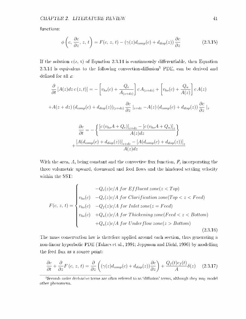
CHAPTER 2. LITERATURE REVIEW 41
functions:
φ
(c,∂c
∂z, z, t
)= F (c, z, t)− (γ(z)dcomp(c) + ddisp(z))
∂c
∂z(2.3.15)
If the solution c(z, t) of Equation 2.3.14 is continuously di�erentiable, then Equation
2.3.14 is equivalent to the following convection-di�usion5 PDE, can be derived and
de�ned for all z:
∂
∂t[A(z)dz c (z, t)] = −
[vhs(c) +
Qe
A(z+dz)
]cA(z+dz) +
[vhs(c) +
Qu
A(z)
]cA(z)
+A(z + dz) (dcomp(c) + ddisp(z))(z+dz)∂c
∂z|z+dz −A(z) (dcomp(c) + ddisp(z))
∂c
∂z|z
∂c
∂t= −
{[c (vhsA+Qe)]z+dz − [c (vhsA+Qu)]z
A(z)dz
}+
[A(dcomp(c) + ddisp(z))]z+dz − [A(dcomp(c) + ddisp(z))]zA(z)dz
With the area, A, being constant and the convective �ux function, F, incorporating the
three volumetric upward, downward and feed �ows and the hindered settling velocity
within the SST:
F (c, z, t) =
−Qe(z)c/A for Effluent zone(z < Top)
vhs(c) −Qe(z)c/A for Clarification zone(Top < z < Feed)
vhs(c) −Qf (z)c/A for Inlet zone(z = Feed)
vhs(c) +Qu(z)c/A for Thickening zone(Feed < z < Bottom)
+Qu(z)c/A for Underflow zone(z > Bottom)
(2.3.16)
The mass conservation law is therefore applied around each section, thus generating a
non-linear hyperbolic PDE (Takacs et al., 1991; Jeppsson and Diehl, 1996) by modelling
the feed �ux as a source point:
∂c
∂t+
∂
∂zF (c, z, t) =
∂
∂z
((γ(z)dcomp(c) + ddisp(z))
∂c
∂z
)+Qf (t)cf (t)
Aδ(z) (2.3.17)
5Second- order derivative terms are often referred to as `di�usion' terms, although they may modelother phenomena.

CHAPTER 2. LITERATURE REVIEW 42
The e�ects of suspended solids compression have also been added based on Kynch's
theory (Fitch, 1983; Font, 1988), and has been found to be important as it improves the
predictive power of the model (De Clercq et al., 2008; Ramin et al., 2014; Van Loosdrecht
et al., 2015; Torfs et al., 2015; Burger et al., 2016). It should be noted that the increased
complexity of the mathematical model in this instance will lead to longer computational
times.
Two dimensional (2-D) clari�er unit modelling
There has been some work conducted to broaden from one dimensional to two dimen-
sional modelling, incorporating radial variations, mainly utilising computational �uid
dynamics (CFD) techniques. This approach results in the incorporation of hydraulic
�ow considerations, such as density currents, turbulence and secondary setting tank
geometry. The main bene�t of 2-D modelling is that it avoids many of the assumptions
made by 1-D modelling as the 2-D models can capture more varied phenomena occur-
ring; however, it is more time consuming. The most frequent application of 2-D models
is towards the improvement of SST geometry design and to optimise performance.
When considering sedimentation tanks where the suspended solids concentration is
limited and suspended solid particles settle individually without interaction with neigh-
bouring particles, Imam et al. (1983) applied a �xed settling velocity and used the mean
particle velocity in their model to simulate �oc interaction during clari�cation. Stamou
et al. (1989) simulated the �ow in a sedimentation tank using a 2-D model, where
they solved the momentum and solid concentration equations; however, these equations
where not connected to account for buoyancy. Adams and Rodi (1990) used the same
model and extended the investigation to also consider the inlet �ow arrangements and
�ow �eld calculations. Further advancement of this work accounted for �occulation
where six di�erent size classes with their respective velocities were considered by Lyn
et al. (1992).
Larsen (1977) applied a simpli�ed CFD model to several secondary clari�ers and demon-
strated the presence of a �density waterfall�. A density waterfall is described as a
phenomenon that causes the incoming �uid to sink to the tank bottom not long after
entering. This phenomenon has since been con�rmed by various authors (Kim et al.,
2005; Goula et al., 2008; Das et al., 2016). Other early work includes work by Shamber
and Larock (1981) and by McCorquodale et al. (1991), who utilised �nite volume
methods to solve their clari�er models, with the latter also using �nite di�erence
methods for the boundary conditions, and Huang and Jin (2010) who provided a

CHAPTER 2. LITERATURE REVIEW 43
numerical model for a type of circular sedimentation basin. Their model included an
optimising element using the tank dimensions based on the sludge raking frequency and
preferred removal e�ciency. The blankets of �oc formed that are held in steady state
are complex and McCorquodale and Zhou (1993) investigated the e�ect of a variety of
solids and hydraulic loads on circular clari�er performance, whilst Zhou et al. (1994)
linked the energy equation with the Navier�Stokes equations to simulate the e�ect of
neutral density and warm water into a clari�er model.
Much research has used CFD simulations in order to describe water �ow and suspended
solids removal in settling tanks for wastewater treatment. Even so, works in CFD
modelling of sedimentation tanks for clean water treatment are limited in literature
(Goula et al., 2008; Dufresne et al., 2009). Koltsaklis et al. (2013) stated that the
physical characteristics of the �ocs may not be as signi�cant in the �ow �eld of clari�ers
for clean water due to the lower suspended solids concentration and larger particle size
distributions than those encountered in wastewater treatment. Their work provides
an insight into the �ow patterns in a clean sedimentation tank which can be used
to investigate novel designs or varying operating conditions, for instance temperature
variation, for production-scale tanks.
2.3.3.1 Flotation tank studies
The �nal type of clari�ers which are considered in this work are �otation units. Flota-
tion is the gravity separation process where gas bubbles attach to solid particles to
cause the apparent density of the bubble-solid agglomerates to be less than that of the
water, hence enabling the agglomerate to �oat. There are three main types of �otation
systems (Reynolds and Richards, 1996): electrolytic �otation, dispersed air �otation
and dissolved air �otation (DAF).
The rest of this sub-section will analyse the main one- and two-dimensional mathemat-
ical models developed in literature for dissolved air �otation, including Table 2.4 that
investigates two key theories of DAF: single collectors collision theory and rise velocity
equation in the separation modelling zone including details on the model bias.
One dimensional DAF modelling
As discussed earlier, dissolved air �otation (DAF) is the most viable as a water treat-
ment �oc separation method. Over the years, several conceptual models have been

CHAPTER 2. LITERATURE REVIEW 44
Figure 2.7: Schematic overview of a dissolved air �otation unit.
developed for DAF and can be classi�ed into two groups: i) based on the single
collector collision theory in laminar �ow conditions (called SCC models); and ii) based
on a kinetic model considering the population balance theory of bubbles and �ocs in a
turbulent �ow condition (called PBT models). The SCC theory treats each bubble as
a single collector of particles and considers them as �white water� blankets. The PBT
approach depicts collisions between bubbles and particles through kinetic expression
using a population balance. Both of these two models divide a dissolved air �otation
(DAF) unit into two zones: contact (reaction) and separation, as shown in Figure 2.7.
The contact zone encourages further attachment between bubbles and particles or �ocs,
while the separation zone promotes clari�cation as bubble/�oc agglomerate �oat to the
surface. Table 2.4 provides a summary of a selection of contributions proposing or using
these models, based on the review by Edzwald (2010).
Single collector collision theory (SCC model)
The SCC theory modelling approach was �rst used in air �ltration models (Edzwald
and Van Benschoten, 1990; Edzwald, 1995), and later adapted to model granular water
�ltration (Haarho� and Edzwald, 2004). The model describes collection of particles
by bubbles in froth �otation and in dispersed air �otation (Edzwald, 2010). The SCC
approach considers within the contact zone, bubbles in the �white water� blanket act
as collectors of particles which accounts for particle transport to the bubble interface.

CHAPTER 2. LITERATURE REVIEW 45
Table 2.4: DAF contact and separation zone models. Adapted with permissions fromEdzwald (2010).
Primary Equation Model Basis Comment Author(s)
Single collector collision model
ηD = 6.18
[kbT
g(ρw − ρb)
]2/3[1/dp]
2(i)
ηI = [(dp/db) + 1]2 − (3/2)[(dp/db) + 1]
+(1/2)[(dp/db) + 1]−1
(ii)
ηS = [(ρp − ρw)/(ρw − ρb)][dp/db]2(iii)
ηT = ηD + ηI + ηS (iv)
np,e
np,i
=
exp−
(32αpbηT φbνbtcz
)db
(v)
1. At dynamic steady state,
blanket of bubbles (white
water blanket) modeled in the
contact zone with a high
bubble number concentration.
1. Assuming plug �ow
hydraulics, performance
equation (Equation (v)) is for
continuous steady �ow
through the contact zone.
(Edzwald and
Van Bens-
choten, 1990;
Edzwald, 1995;
Haarho� and
Edzwald, 2004)
2. Bubble acts as collectors. 2. Particle trajectory analysis
does not incorporate
interparticle forces, which can
be attributed to London-van
der Waals and electrostatic
force.. Short range
hydrodynamic e�ect of water
layer model. All of these
e�ects are accounted for
between bubble and particle
not considered in in the
empirical attachment
e�ciency term apb.
3. Particle transport terms
expressed with respect to the
single collector e�ciencies.
Expressions for interception
(nI), settling (ns) and inertia
(not shown since not
important for DAF) developed
from particle trajectory
analysis. Brownian di�usion
(nB) expression is obtained
from Stokes-Einstein
relationship.
Rise velocity equation for Floc-bubbles aggregates
vfb = 4g(ρw − ρb)df b2/3kµw (vi)
where
dfb = (d3f +Nbd
3b)
1/3(vii)
ρfb = ρfd3f +Nbρbd
3b/d
3b +Nbd
3b (viii)
vfb = (4/3K)0.8
[g0.8
(ρw − ρf b)0.8df b
1.4
/(ρw)0.2
(µw)0.6
] (ix)
vfb = Nbgρwd3bϕ
0.5/18µwdfb (x)
vfb = gρwd3bϕ
0.5/18µw(d
3b + jd
3f )
1/3(xi)
1. Equation (vi) for Re ≤ 1,
holds at 20°C for dfb ≤160
µm with 4 attached 100 µm
bubbles. K accounts for the
shape of the aggregate and its
e�ect on increased resistance
to drag.
(Haarho� and
Edzwald, 2004)
2. Equation (ix) for transition
zone Re 1 � 50.
(Matsui et al.,
1998)
3. For Equation (x) Re ≤ 1
and applies to case of large
number bubbles attached to
each �oc.
4. For Equation (xi) Re ≤ 1
and applies to case of �oc size
smaller than bubble size and
multiple �ocs (j) can be
attached to each bubble.

CHAPTER 2. LITERATURE REVIEW 46
Also, in this approach, the e�ect of streamlines of �ow diverting around the bubble
is considered and an expression for interception and settling is derived from particle
trajectory analysis. The inter-particle forces are not considered in SCC e�ciency (ηT ),
so whether potential collisions are successful resulting in attachment is accounted for
by an empirical coe�cient αpb.
Separation zone modelling
The bubbles in the contact zone are smaller than the bubbles in the separation zone.
This is due to coalescence or even due to reduction of water pressure as the bubbles
move from the bottom of the contact zone toward to the surface and into the separation
zone (as shown in Figure 2.7). The main focus in the separation zone is the rise velocity
for �oc-bubble aggregates, and these factors can be modelled based on the Hazen theory
which is similar to the sedimentation tank theory (Edzwald, 2010). The earlier models
of separation zone for DAF systems assumed a vertical plug �ow from the surface to
the underdrain system. Strati�ed �ow was explained as water travelling in a horizontal
�ow layer along the top of the tank to the far end, and then travelling back towards
the front in a second horizontal layer below the �rst layer. Models predicting strati�ed
�ow often employ CFD techniques, but are limited as they do not identify the desired
strati�ed �ow conditions and do not predict the quantitative impact of the strati�cation
on bubble removal (Lakghomi et al., 2012). Hedberg et al. (1998) and Amato et al.
(2001) conducted empirical studies that suggest improvements in the removal of single
bubbles in the separation zone can be achieved by producing larger bubble aggregates
that have a higher rise velocity. This �nding is in agreement with those of Edzwald
(2010) and Leppinen and Dalziel (2004) who also found that removal e�ciency was
improved with large bubble aggregates in the separation zone.
Two dimensional (2-D) DAF modelling
As for models of other clari�ers, the prediction capabilities of DAF models can be
improved by using CFD techniques to show how the velocity of the water �ow changes
as a function of �ow rate, water temperature, aspect ratio, size of the tank, and ba�e
height . Several authors have stated how CFD can be used as a design tool (a list can
be found in Edzwald (2010)). Amato and Wicks (2009) report by considering the e�ects
of the ba�e height on water velocities and bubble concentration in the separation zone,
CHAPTER 2. LITERATURE REVIEW 47
CFD can be used to evaluate a plant expansion by increasing the �ow of an existing
DAF tank.
Previous CFD models of DAF units, such as those reported by Kwon et al. (2006),
Amato and Wicks (2009) and Edzwald (2010), neglected bubble aggregation and were
based on the assumption of a uniform bubble size. Looking at other application of CFD
studies, such as mining, have used population balance algorithms to describe bubble
coalescence and break-up (Edzwald, 2010; Chen et al., 2004) and it is predicted that the
inclusion of bubble aggregation in a CFD model would make the model more accurate.
While CFD is a useful design tool, few veri�ed models exist. There are assumptions
about the bubbles that have to be made about; for example, as the bubble size signi-
�cantly a�ects the predictions. Also, due to the di�culty of including the solid phase,
this phase is usually neglected; although in practice, the solid phase particles a�ect the
velocity predictions and air bubble concentrations. Currently, there is more research
being conducted in order to develop a robust CFD model (Lakghomi et al., 2015;
De Souza Vasconcelos et al., 2015; Samstag et al., 2016).
Summary and outlook
Flocculation clari�er and dissolved air �otation are the main clari�cation processes
utilised for clean water treatment. There have been numerous advances in the develop-
ment of mathematical models that capture the phenomena occurring. Kynch's model
of sedimentation (Concha and Bustos, 1991) has been used as a starting point for many
sedimentation models throughout the years. Extensions have been made to the model
to simulate batch and continuous sedimentation within cylindrical columns, many of
the models utilise macroscopic balances. The sedimentation process in the secondary
settling tank is commonly approached from one-dimensional modelling. Several authors
have attempted to extend the models to incorporate more detailed physical phenomena
in order to enable a more robust and accurate model (Concha and Bustos, 1991; Burger
and Concha, 1998; Burger et al., 1999). The �otation models consider a number of
phenomena which are of great importance in plant operation, and however, are therefore
very complex and require a number of parameter values which can only be obtained
from experimental data or �tted from plant data. Therefore unfortunately limiting their
current applicability. As pointed out by Edzwald (2010), more research is needed on the
magnitude of bubble coalescence, collisions and attachment, and �oc detachment that

CHAPTER 2. LITERATURE REVIEW 48
may occur in DAF units and how these e�ects should be incorporated into mathematical
models.
There has been a substantial amount of mathematical modelling research in the wastewa-
ter industry focusing on the development of a robust secondary settler tank, which has
be applied to a sludge clari�cation unit in the clean water industry (Clarke et al.,
1978; Wilson et al., 1979; Head et al., 1997). This brings encouragement in the
application of this mathematical modelling approach to the clean water industry as
it becomes an emerging research area. One-dimensional models of �occulation clari�ers
(sedimentation tanks) are promising as they are able to be developed to accurately
represent areas of interest at a reduced computational time than a two-dimensional
model.
2.3.4 Filtration
The purpose of �ltration in water treatment is the removal of solid particles from the
water by passing the solid/water mixture through a porous medium or other suitable
material to capture the solid particles whilst allowing the water to pass, thus achieving
the required quality of �ltered water. This unit is usually the third physical unit in
the water treatment process and is often the last line of defense to remove �oc and
colloidal particles from entering the distribution by retention in the porous medium. A
porous medium is a solid matrix containing voids which interconnect to enable the �uid
�ow through the medium at a low speed (Jegatheesan and Vigneswaran, 1987). Upon
�ltration, the media thereby retains most of the solid matter within the pore structure.
There are three basic types of �ltration methods used in water treatment: slow sand
�lters (Huisman and Wood, 1974), rapid gravity �lters (Han et al., 2008) and pressure
�lters (Landman et al., 1995), with rapid gravity �lters being the most common. Slow
sand �lters are the oldest and original type of sand �lter. These �lters operate at
low-loading rates and thus they are deemed as `slow'. In this type of �lter, two processes
are used to treat the water: physical straining and biological action using �ne sand as
a medium, where at the top of the sand and the uppermost part of the sand bed there
is a layer of biological growth (also known as schmutzdecke), which is vital for e�ective
operation.
Rapid gravity �lters di�er from slow sand �ltration as they operate at high loading rates
using a coarser media with a high permeability rate. In this type of �ltration, water
CHAPTER 2. LITERATURE REVIEW 49
is treated by physical treatment alone and the media used can be granular activated
carbon. Pressure �lters share many of the same characteristics as rapid gravity �lters
except that they operate under pressure in a large closed vessel. They can be situated
either vertically or horizontally with a set of frontal pipe work and valves. Slow sand
�lters and rapid sand �lters are widely used for the removal of suspended solids present
in water, but sand �lters have a number of limitations and drawbacks such as high
energy requirements for back-washing. One of the most serious problems involved with
sand �lters include maintaining bed homogeneity during operation. Inhomogeneities in
the bed leads to formation of channels in the bed, poor distribution of the liquid �ow
through the bed, and thus very low particulate removal (Brika, 2010). The advantages
and disadvantages of the various �lter types can be found in Table 2.5.
A comprehensive review of granular media �ltration processes is provided by Cleasby
and Logsdon (1999). The various types of �lters used for particle removal in potable
water �ltration can be classi�ed based on several factors, including (Tobiason et al.,
2010):
1. Dominant overall mechanism for particle removal: Particle removal mech-
anisms can be divided into three main classi�cations: deep bed �ltration, straining
�ltration, and cake �ltration. Deep bed �ltration occurs when the pore spaces of
a �lter receive particle deposits which transport to, and attach themselves on, the
surface of the granular media. Straining �ltration occurs when the particle is too
large to pass through the pore opening; and this type of �ltration is predominantly
used in low pressure membrane �ltration. Cake �ltration is when water to be
�ltered passes through a cake comprised of previously deposited particles.
2. Filtration media used: The �ltration media used are comprised of speci�c
depths of one or more types and sizes of granular media, such as rapid sand,
dual-media and slow sand �lters.
3. Hydraulic loading rate: The hydraulic loading rate is the �ow rate of water
applied per unit area of the �lter. It is the velocity of the water approaching
the face of the �lter. It has a signi�cant impact on the capital cost of treatment
because the required �ltration surface area to produce a desired �ow decreases as
the hydraulic loading rate increases.
In water and wastewater treatment, particles of various sizes present in water can
be removed by deep bed �ltration, which involves complex mechanisms. In order for

CHAPTER 2. LITERATURE REVIEW 50
Table 2.5: Advantages and disadvantages of various �lter types used in clean watertreatment.
Advantages Disadvantages Author(s)
Slow sand �ltration Works withoutcoagulants.
Produces excellent waterquality.
Low cost and ease of
construction/operation.
Large area required.
Labour intensive tooperate.
Not e�ective with highlyturbid waters.
Algal growths cause
operational di�culties.
(Huisman and
Wood, 1974)
Rapid gravity �ltration Low construction costs.Produces excellent waterquality (quality is stillless than slow sand�ltration).
Operation and backwash
can be observed.
Increased operation costs.
Increased maintenance.
(Han et al.,
2008)
Pressure �ltration Placed directly inpumping line with littlehead loss.Produces good waterquality.
Low initial costs.
Unable to observe the�lter media.
Unable to determine the
operating condition of the
media as it changes.
(Landman
et al., 1995)
Membrane �ltration Good degree oftreatment.Produces good waterquality.
Operation and
maintenance is simple.
Regular maintenance. Crittenden
et al. (2012)
removal to be e�ective, there are various factors to be considered such as physical and
chemical characteristics of the water, the particles and the �lter medium (Vigneswaran
et al., 2009).
Stages of deep bed �ltration
The �ltration process can be categorised into two stages: the initial stage and the
transient stage. The initial stage is when the �lter bed is clean and particle deposition
occurs onto the clean �lter, which has a negligible e�ect on the properties of the �lter
during the initial stage. The transient stage describes the rest of the �ltration process.
Where deposition occurs on �lter grains which are already partly covered by deposited
particles. Depending on the chemical conditions of the suspension and �lter medium,
the removal of particles can either improve or degenerate during this stage.

CHAPTER 2. LITERATURE REVIEW 51
Figure 2.8: Typical curve showing �lter performance over di�erent stages of transient�ltration. The relative suspended solid particle concentration, c/c0 is shown over time,t (Vigneswaran et al., 2009).
Figure 2.8 shows the three sub-stages that occur in the transient stage during a �lter run,
which are the ripening stage, working stage and breakthrough stage. The improvement of
the �lter quality (c/c0) with time is shown in the ripening stage, followed by the working
stage in which the particle removal remains essentially constant. Finally, in the latter
part of �ltration, the breakthrough stage occurs where the particle removal starts to
deteriorate and the �lter e�ciency decreases with time, at this time a back-washing
occurs and resets the unit to the ripening stage.
For water �ltration, there are a wide range of options that are available and have
been presented in literature. Deep bed �ltration dominates the main research area
in which both macroscopic (deal with the accumulative collection of deposits) and
microscopic (considers the size of the individual particle as well as the number of
particles) approaches have been considered. Equations used to describe phenomena
based on a macroscopic and microscopic approaches are discussed in this section. Very
few �ltration models have been formulated where �ltration back-washing to clean the
�lter medium occurs in order to restore the e�ciency of the �ltration unit. However,
optimum conditions and the e�ects of surface properties are also discussed in this
section.
2.3.4.1 One-dimensional modelling
There have been various mathematical models that have been developed to describe
particle capture in a �lter (Rajagopalan and Tien, 1976; O'Melia and Ali, 1978; Johnson
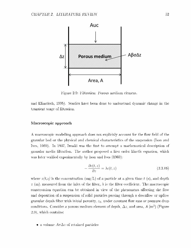
CHAPTER 2. LITERATURE REVIEW 52
Figure 2.9: Filtration: Porous medium element.
and Elimelech, 1995). Studies have been done to understand dynamic change in the
transient stage of �ltration.
Macroscopic approach
A macroscopic modelling approach does not explicitly account for the �ow �eld of the
granular bed or the physical and chemical characteristics of the suspension (Ison and
Ives, 1969). In 1937, Iwaski was the �rst to attempt a mathematical description of
granular media �ltration. The author proposed a �rst order kinetic equation, which
was later veri�ed experimentally by Ison and Ives (1969):
− ∂c(t, z)
∂z= λc(t, z) (2.3.18)
where c(t,z) is the concentration (mg/L) of a particle at a given time t (s), and depth
z (m), measured from the inlet of the �lter, λ is the �lter coe�cient. The macroscopic
conservation equation can be obtained in view of the phenomena a�ecting the �ow
and deposition of a suspension of solid particles passing through a down�ow or up�ow
granular depth �lter with initial porosity, ε0, under constant �ow rate or pressure drop
conditions. Consider a porous medium element of depth, ∆z, and area, A (m2) (Figure
2.9), which contains:
� a volume Aσ∆z of retained particles
CHAPTER 2. LITERATURE REVIEW 53
� a volume Aεc∆z of moving particles entrained by the liquid
� a deposit of real volume Aβσ∆z imprisoned by the retained particles
where σ is the speci�c deposit of particles (mg/L) onto the �lter medium expressed
in terms of the ratio of the volume of deposited material over the di�erential volume
under consideration (-), c is the volumetric concentration of particles within the zone
(mg/L), ε is the porosity (-). With varying assumptions, the rate of particle deposition
can be written in terms of the speci�c deposit, σ, or the particle concentration, c:
∂σ
∂t= λuc (2.3.19)
The governing parameters of the macroscopic model, the �lter coe�cient, λ, and the
speci�c deposit, σ, are implicit functions of the physical and chemical characteristics,
such as attachment and transport e�ciency between particles and to the �lter, of the
suspension and �lter medium, as well as of �ltration velocity, u. The parameters vary
with time and �lter depth during the �ltration process (as shown in Figure 2.8). In
order to predict the concentration pro�le, the value of the �lter coe�cient λ must �rst
be estimated. Yao et al. (1971) used the theory of �oc formation of Smoluchowski
(as outlined in subsection 2.3.2) as a basis to determine the clean bed �ltration rate
λ0. Prior to this work, several authors tried to determine the clean bed �ltration
rate λ0 in an empirical way for di�erent circumstances. The main limitation of the
macroscopic approach is that the physical and chemical characteristics of the �lter
medium, the suspension and the �occulants used are not explicitly described. This is
where microscopic modelling will be bene�cial to provide some solutions to the current
limitations in macroscopic modelling.
Microscopic approach
In a microscopic modelling approach, the �lter bed is modelled as a gathering of single
or unit collectors, which �uid �ows around or through the �lter bed. In porous media,
as a particle approaches a media grain, the motion deviates from the streamline due
to di�erent forces and torques acting on the particles, mainly related to transport
and attachment. The main transport mechanisms are sedimentation, interception,
Brownian di�usion and hydrodynamic action (Keir et al., 2009), as illustrated in Figure
2.10.

CHAPTER 2. LITERATURE REVIEW 54
Figure 2.10: Basic transport mechanisms in a granular �lter (Binnie and Kimber, 2009;Tobiason et al., 2010).
� Sedimentation takes into account the gravitational forces on the particles to be
removed. If the density of the particle is greater than that of water, the dense
particles will be removed more e�ectively by settling to the bottom of the unit.
� Interception occurs when particles moving uniformly collides with a grain of �lter
media. This enables the particle to be captured, thus being removed from the
liquid �ow.
� Brownian di�usion is a random movement observed due to the thermal agitations
of the �uid molecules, which a�ects very small particles suspended in the medium.
� Hydrodynamic action arises from a random drifting across the �ow streamlines
which may lead to contact with the �lter grain surface. Flow through the �lter
bed is typically laminar with some velocity pro�le, and hence a shear �eld. For
a uniform shear �eld and a spherical particle, rotation of the particle causes a
curving path across the shear �eld. For non-uniform shear �eld and non-spherical
particles (which is most common in practice), the particle is de�ected in a similar,
but unpredictable manner. This is due to the velocity gradient in each pore
surrounding the grains of �lter media. A small particle passing through a grain
of �lter media will tend to be rotated by the velocity gradient. This will cause
pressure di�erences across the particle, which will move it towards the �lter media.

CHAPTER 2. LITERATURE REVIEW 55
Figure 2.11: Particle attachment to �lter media and to other particles.
A detailed discussion of these mechanisms can be found in Jegatheesan and Vigneswaran
(2003). The authors state that these mechanisms are likely to occur simultaneously as
particles in a �owing suspension will be subject to some or all of the mechanisms
at varying degrees, and the level of impact will depend on �uid �ow conditions, the
geometry of the �lter pores and the nature of the particles.
Figure 2.11 shows that once a suspended solid particle has made contact with the
�ltering media, it needs to be retained by an attachment mechanism to stick to the
media. In the literature, the attachment mechanisms are considered to be gravity,
London-van der Waals attraction, and double-layer forces (Keir et al., 2009). Adin
and Rebhun (1974) state that the e�ciency of a �ltration process for a speci�c set
of hydraulic conditions depends on the attachment forces and can be described by a
relationship between attachment and shear forces. As the hydrodynamic shear forces
become greater than the attachment forces, breakthrough of suspended solid particles
occurs.
Transport e�ciency, η, is de�ned as the fraction of contacting for a given collector
relative to the particles approaching (Elimelech and O'Melia, 1990). Elimelech and
O'Melia (1990) list the common equations for collection e�ciency, with the most com-
mon correlation being the one developed by Rajagopalan and Tien (1976). Their
studies were developed further to incorporate back-washing, and can be used to estimate
when the best back-washing time would be (Fitzpatrick, 1998; Brouckaert et al., 2006).
Back-washing involves reversing the �ow of water through the �lter in order to �uidise
the bed and lift the particle building up on the �lter medium and sending them to

CHAPTER 2. LITERATURE REVIEW 56
drain. This is important not only for the maintenance of the �lter but also for the �lter
e�ciency by restoring the ripening stage of the �lter cycle. Brouckaert et al. (2006)
show that the particle/�lter grain transport e�ciency in the clean �lter, η0, can be
calculated from:
η0 = 4A1/3s Pe
−2/3 + AsN1/8LON
15/8R + 3.38x 10⁻³AsN
1.2G N−0.4
R (2.3.20)
where
As =1 (1− p5)
w(2.3.21)
w = 2− 3p+ 3p5 − 2p6 (2.3.22)
p = (1− ε)1/3 (2.3.23)
The �rst term on the right hand side in Equation 2.3.20 represents �ltration due to
Brownian di�usion. As is a parameter de�ned by the Equation 2.3.21; and Pe is
dimensionless Peclet number given by D∞/udc, where D∞ is the bulk particle di�usion
coe�cient (m2/s), u is the super�cial velocity (m/s) and dc is the clean �lter grain
diameter (m). The second and third terms represent the combined e�ects of interception
and gravity when the retardation and London-van der Waals attraction are included.
w and p are parameters de�ned by the Equations 2.3.22 and 2.3.23, respectively; NLO
is dimensionless van der Waals number given by 4A/9πµd2pu, where A is the Hamaker
constant (1 x 10⁻²⁰J), µ is the viscosity of water (Pa. s) and dp is the suspended solid
particle diameter (m); NR is the dimensionless ratio of particle to collector size given
by dp/dc; and NG is the gravitational force number given by (ρp−ρ)gd2p/18µu, where ρp is
the particle density (kg/m3) and g is gravity (m/s2).
Model for transient stage of �ltration
Within the microscopic approach, There are a variety of models that have been de-
veloped to calculate particle capture in a �lter. Table 2.6 presents a summary of the
most cited models in the literature which predict the removal e�ciency during transient
condition of a �lter, and lists their strengths and weaknesses.
Although �ltration models can be used very e�ectively to assess the in�uence of each
variable, such as �lter velocity, on �lter performance, they all have several similar
weaknesses:
� Existing models are based on the attachment of spherical particles on a single size

CHAPTER 2. LITERATURE REVIEW 57
Table 2.6: Summary of recent �ltration models and their strengths and weaknesses.
Models Strengths Weaknesses Author(s)
Detachment
mechanisms
Can simulate �lter
performance satisfactorily
and easily at all �ltration
velocities.
Inclusion of factors
relating to the attraction
in the transient state
modelling in an explicit
manner is required.
(Jegatheesan, 1999;
Han et al., 2008)
Filtration and
adsorption
Can simulate �lter
performance
satisfactorily.
Only at low �ltration
velocity.
(Jegatheesan,
1999)
Retained particles
blocking other
particle collection
Based on random
sequential adsorption
mechanism, which can be
used to predict the
transient stage and
deposition of colloids.
Cannot be applied for
unfavourable surface
condition.
(Johnson and
Elimelech, 1995)
E�ects of change in
the surface charge
of �lter grains
Useful in predicting the
accumulation on the �lter
grain surface due to the
deposition of particles.
Model is valid in
predicting the changes in
the �lter media structure
only at low inception
numbers.
(Jegatheesan and
Vigneswaran, 2003)
spherical media grain. Media characteristics such as angularity or media range
based on the e�ective size has not been considered but is clearly of importance
as neglecting this means hydrodynamic forces are not being represented.
� The studies mentioned in the table consider only deep bed �ltration which, for
applications in the developed world, is the main option However, in emergency
scenarios where pre-�ltration treatment is not a likely option, minimising the
e�ect of surface straining in order to keep the �ltration system e�cient can be of
equal importance to optimising depth �ltration (Rajagopalan and Tien, 1976).
Model for �ltration back-wash
Filtration operation involves back-washing to clean the �lter medium. As stated earlier,
backwashing involves reversing the �ow of water through the �lter in order to �uidise
the bed to lift the particles building up on the �lter medium and send them out to the
drain. This is important not only for the maintenance of the �lter but also for the �lter
e�ciency by restoring the ripening stage of the �lter cycle. Numerous research e�orts
have been made in studying the behaviour of �uidised beds (which is the phenomena

CHAPTER 2. LITERATURE REVIEW 58
occurring during back-wash) because of their use in the chemical and mineral processing
industry (Amirtharajah, 1971; Kawamura, 1975; Huang and Basagoiti, 1989; Ahmad,
1996; Brouckaert, 2004). There have been several modelling attempts to predict the pro-
cess of �ltration back-wash, including predicting the conditions for optimum backwash
(Amirtharajah, 1971; Kawamura, 1975) and determining the e�ect of surface properties
for �oc, clay and bacteria on the e�ciency of backwash (Huang and Basagoiti, 1989;
Ahmad, 1996). However, Brouckaert (2004) states that the main limitations of existing
back-wash models is that they do not su�ciently account for the intense mixing that
occurs at the beginning of backwash as the most clogged regions of the �lter bed collapse
and disintegrate. This is due to the di�culty in capturing the initial stage because the
mixing conditions change very rapidly with time.
Headloss development
Headloss in a �lter bed is an important factor for the �lter bed conditions, and can
be used as an indicator to start �lter washing. Headloss through the �lter media is
usually monitored by di�erent pressure-cell devices that measure the water pressure
above and below the �lter media. When terminal headloss is reached, the �lter should
be washed, otherwise turbidity breakthrough may occur. One of the most practical
headloss monitoring methods is to measure the headloss at di�erent depths within the
�lter bed with several pressure taps (Crittenden et al., 2012).
For a clean bed, the pressure drop across the �lter bed is given by the Carmen-Kozeny
equation. This equation was derived assuming that the �ow is laminar, the �lter media
are uniform spheres, and the pressure drop results entirely from the form-drag loss as
�uid moves around the media. The Carmen-Kozeny equation can be expressed as a
change in headloss over a length of clean �lter bed:
− ∆P
L=
150µu (1− ε0)2
d2cε
3o
(2.3.24)
The pressure drop after a backwash can be expressed as:
∆P = hρg = L (ρs − ρ) g (1− ε) (2.3.25)
where 4P is pressure drop, h is the headloss (m), L is the �lter bed depth (m), u is
the super�cial velocity (m/s) and µ is the viscosity of water (Pa. s). Equation 2.3.24

CHAPTER 2. LITERATURE REVIEW 59
predicts that the headloss should increase as a function of decreasing grain diameter,
increasing super�cial velocity, increasing viscosity and decreasing density of the in�uent.
It is bene�cial to factor in headloss when looking to model �ltration performance.
Summary and outlook
Filtration is generally the �nal physical removal process in clean water treatment. This
is achieved by passing a mixture of suspended solid particles and water through a porous
medium to capture the solid particles whilst allowing the water to pass. Tobiason et al.
(2010) provide a list of the various �lters that can be used and classi�ed by several
factors with the dominant overall mechanism for particle removal being highlighted.
For water treatment, the preferred mechanism is deep bed �ltration. Numerous models
have been proposed to predict the removal e�ciency in deep bed �ltration at initial and
transient stages and at both macroscopic and microscopic levels. In general, �ltration
models based on the concept of adsorption can simulate the �ltration performance at
low �ltration velocity (Ali and Gupta, 2006) whereas models based on the detachment
mechanism (Jegatheesan, 1999; Han et al., 2008) can simulate the �lter performance
acceptably and easily at all �ltration velocities. The detachment mechanisms can also
be used to show the three stages that usually occur during a �ltration run: ripening,
working and breakthough stages, which enables e�ective timing for back-washing.
In order to develop a more detailed predictive model of back-wash e�ciency, the model
should be based on easily measured parameters such as rate of headloss development,
which is an important indicator for all the �lter bed conditions. Headloss can be used
as an indicator to start �lter washing, initiating turbidity decrease through removal of
total suspended solids (�ocs) and �lter run time. Such a model can be easily integrated
with existing models of the �ltration phase of the �lter cycle, including models of �lter
ripening.
2.3.5 Disinfection
Disinfection is the �nal main unit operation in clean water treatment before the water
enters the distribution system. In this process, most of the remaining pathogenic organ-
isms are killed or controlled. The most commonly used disinfection treatment systems
are ozonation, ultraviolet irradiation (UV) and chlorination using chemicals such as
chlorine dioxide and chlorine based compounds. UV water treatment is an e�ective

CHAPTER 2. LITERATURE REVIEW 60
Table 2.7: Advantages and disadvantages of various disinfection treatment used in cleanwater treatment.
Advantages Disadvantages Author(s)
Ozonation Utilises a short contact time.Ozone decomposes rapidly so noharmful residuals.Ozone is generated on site, thus,fewer safety problems withshipping and handling.
Increases dissolved oxygen
concentration of the e�uent.
Low dosages may not e�ectivelyinactivate some viruses, sporesand cysts.
Requires complicated equipmentand e�cient contacting systems.
Corrosion resistant material isrequired.
O� gases must be destroyed to
prevent exposure.
(Weiss, 1935;
Am Water
Works Res
et al., 1991;
Reynolds and
Richards, 1996)
Ultraviolet irradiation
(UV)
Physical process, whicheliminates the need to generate,handle, transport or store toxicchemicals.User friendly for operators.
Utilises short contact time.
Equipment requires less space
than other methods.
Low dosage may not e�ectivelyinactivate some viruses, sporesand cysts.
Potential for bacterialreactivation.Cleaning method to preventfouling.
Not cost-e�ective.
(Linden and
Rosenfeldt,
1990; Reynolds
and Richards,
1996)
Chlorine Cost e�ective.Well established technology.
E�ective against wide spectrumof pathogenic organisms.
Flexible dosing control.
Eliminates odours.
Toxic to aquatic life.
Highly corrosive.
Chlorine reacts with someorganic compounds that createmore hazardous compounds.
Low doses of chlorine will not
be able to inactive all parasitic
species, due to resistance.
(Reynolds and
Richards, 1996;
Clark et al.,
2001)
way to disinfect drinking water supplies, and this process is becoming increasingly
popular as an alternative to chlorine disinfection systems as no chemicals are added
to the water. Details of the advantages and disadvantages of ozonation, ultraviolet
irradiation and forms of chlorine can be found in Table 2.7.
For water disinfection, there are a wide range of options that are available and have
been presented in literature. Due to the complex phenomena occurring most modelling
within this area are empirical models and the development of these are discussed in this
section.
2.3.5.1 Kinetic model
Several authors have proposed mathematical models of disinfection based on empir-
ical observations (Lawrence and Cappelli, 1977; Hijnen et al., 2006). More detailed

CHAPTER 2. LITERATURE REVIEW 61
modelling approaches have also been considered, in particular, kinetic modelling which
simpli�es and idealises complex phenomena occurring within a system. Based on the
following assumptions being satis�ed, kinetic inactivation models are derived (Lawrence
and Cappelli, 1977; Gyurek and Finch, 1998; Hijnen et al., 2006):
1. No back mixing.
2. Uniform dispersion of disinfectant molecules and organisms.
3. Su�cient mixing to ensure liquid di�usion is not rate limiting.
4. Fixed temperature and pH.
5. Constant disinfectant concentration during the contact time.
These assumptions have been applied to the various disinfection methods available.
Several kinetic models have been derived from the following di�erential rate law:
dN
dt= −kmNxcntm−1 (2.3.26)
where dN/dt is the rate of inactivation of microorganisms, k is reaction rate constant
found experimentally, N is the number of microorganisms that did not inactivate at
contact time t, c is the concentration of disinfectant and m, n, and x are empirical
constants. Table 2.8 presents a summary of kinetic models that are currently available.
The equations presented in this table are used to describe the inactivation of microor-
ganisms within disinfection techniques and all equations are applicable to chlorination,
ozonation and ultraviolet irradiation.
Chlorination
A representation of second-order kinetics for chlorine consumption in disinfection was
developed by Zhang et al. (2000), who incorporated chlorine consumption into a numer-
ical model to predict the formation of disinfection by-products (DBP) for clean water
applications. The model was re�ned to predict the required chlorine demand in the
disinfection process. The main concern was the distribution of the major DBPs in the
contact tanks, this includes primarily total trihalomethanes (TTHMs), dichloroacetic
acid (DCAA) and trichloroacetic acid (TCAA).

CHAPTER 2. LITERATURE REVIEW 62
Table 2.8: Summary of all kinetic inactivation models for disinfection. Reproducedwith permissions from Gyurek and Finch (1998).
Primary Equation Model Basis Comment Author(s)
Chick-Watson
−kCnT
1. Disinfectant is presentin excess.2. Reaction isirreversible.
3. The microorganisms
are genetically similar.
1. The simplicity of theChick-Watson modelmakes it attractive fordesign and regulatorypractice.
2. Can adequately
describe ultraviolet
radiation.
(Chick,
1908;
Watson,
1908)
Hom rational
−kCnTm
− log[1 +Nx−10 (x− 1)kCnT ]
(x− 1)
Can describe the shoulder
and tailing o� phenomena
(which are part of the
three-stage inactivation
curve: shoulder, linear
and tailing) for x < 1 and
x > 1.
Model created by
observing that plots of log
survival on contact time
for chlorine disinfection of
natural algal-bacterial
systems were curvilinear
rather than linear.
(Hom, 1972;
Majumdar
et al., 1973;
Roy et al.,
1981)
Hom-Power law
− log[1 +Nx−10 (x− 1)kCnTm]
(x− 1)
Model may provide better
�t than either the Hom or
Rational model for
survival curves in which
the inactivation rate
initially increases and
then decreases during the
contact time.
A kinetic model with as
many as four parameters
can lead to
over-parametrisation
resulting in highly
correlated parameter
estimates.
(Anotai,
1996)
Selleck
−nlog[1 + CT
k]
Proposed when a
decrease in inactivation
rate during contact time
occurred even when the
disinfectant concentration
remained constant.
Model has been used to
describe survival curves
having an initial shoulder
and a declining
inactivation rate, which
are often observed in
chlorination of
wastewater.
(Gard, 2008;
Selleck
et al., 1978;
Haas, 1979)

CHAPTER 2. LITERATURE REVIEW 63
Table 2.8 continued: Summary of all kinetic inactivation models for disinfection.Reproduced with permissions from Gyurek and Finch (1998).
Primary Equation Model Basis Comment Author(s)
Multiple target
log[1− (1− e−kCT ))nc ]
Mixed second-order
kinetics describe the rate
of inactivation of a
critical target.
The multiple-target
model is not suitable for
describing microbial
inactivation kinetics
because it is unlikely
clumps will be of equal
size and cell damage will
be randomly distributed
among targets.
(Kimball,
1953; Wei
and Chang,
1975)
Series event
−kCT + ln[∑l−1
k−0(kCT )k
k!
]ln(10)
1. Series-event modelassumes that a number of�rst-order reactions withrespect to concentrationare needed to inactivatethe organism.
2. Series-event model
describes shoulder
behaviour when l > 1.
Inappropriate because the
series-event model
assumes that the
occurrence of an event in
a viable organism is
independent of the
occurrence of previous
events.
(Wei and
Chang, 1975;
Severin
et al., 1984)
Multiple series event
log
[1−
(1− e−kCT
l−1∑k=0
(kCT )k
k!
)]Multiple series-event
model simpli�es to the
multiple-target model
when uniform clumps are
assumed to be made of
single-hit organisms.
Possible to describe
tailing-o� behaviour (seen
in graphs) using a
number of multiple
series-event models, each
corresponding to a
di�erent clump size L,
the complexity in doing
so limits the applicability
of the series-event model.
(Wei and
Chang, 1975;
Severin
et al., 1984)

CHAPTER 2. LITERATURE REVIEW 64
Clark et al. (2001) presented a mathematical model based on the use of two second-order
terms for predicting chlorine consumption loss or decay. It was found that the water
quality variables needed to predict the model parameters, in order of importance, where:
initial chlorine concentration, UV absorbance, total organic carbon (TOC) concentra-
tion, pH, bromide concentration, and alkalinity. More recent research conducted by
Muslim et al. (2009), provided a dynamic single-input single-output model based on
CFD to describe chlorine dosing and the decay process in chlorine contact tanks. The
model provided a new direction in evaluating a control scheme particularly pertinent
to �uid mixing problems.
Ozonation
Weiss (1935) presented two analytical kinetic ozone decomposition models for ozone
decomposition in water. The �rst model was called Staehelin, Hoigne and Buhler
(SHB), and was experimentally developed for acidic to neutral pH conditions. With
an empirical approach, Lovato et al. (2009) developed the SHB model by relating the
pH solution to one of the 18 kinetic constants. The Tomiyasu, Fukutomi and Gordon
(TFG) model, on the other hand, considered high pH values (Audenaert et al., 2010).
Westerho� et al. (1997) compared both models and found that they predicted di�erent
kinetics for molecular ozone, HO radicals, and other intermediate species; however,
both models were able to predict similar O3/HO ratios.
Ultraviolet irradiation
Di�erent approaches to modelling ultraviolet irradiation (UV) in water treatment have
been considered in the literature: 1) the disinfection �eld is considered as a continuum
and solved in an Eulerian framework, and 2) the microorganism particles and their
inactivation are tracked using a Lagrangian frame of reference. There have been several
studies that suggest the e�cacy of UV inactivation can occur due to photoreactiva-
tion of the damaged microorganism (Eker et al., 1991; Whitby and Palmateer, 1993;
Lindenauer and Darby, 1994; Chan and Killick, 1995).
Photoreactivation is the phenomenon by which UV-inactivated microorganisms recover
activity through the repair of dimers in the DNA under near-UV light (Oguma et al.,
2001). Few papers have focused on modelling the reactivation processes, which focus on
describing qualitative studies of the process (Harris et al., 1987; Lindenauer and Darby,

CHAPTER 2. LITERATURE REVIEW 65
1994; Hassen et al., 2000; Oguma et al., 2004). There are other authors who have tried
to model both the reactivation and inactivation phases by comparing experiments that
did and did not include reactivation (Tosa and Hirata, 1999; Beggs, 2002). Kashimada
et al. (1996) o�ered a model to predict the reactivation phase independently, but the
experiments carried out were insu�cient to be generalised, and a better understanding
of the factors a�ecting the kinetics of activation is therefore required. There have also
been studies suggesting numerical simulations based on exploiting techniques from CFD
can be utilised in the modelling e�orts for UV disinfection (Lyn et al., 1992). Lyn et al.
(1992) used a steady state two-dimensional depth averaged model to predict the turbu-
lent �ow in a vertical-type open channel UV reactor. The model was extended by Lyn
(1999) compared numerical predictions with experimental measurements and examined
in more detail the simulation of not only �ow, but also disinfection in open-channel UV
disinfection systems.
Summary and outlook
The disinfection of water treatment plants is mainly a chemical process, nevertheless a
process model would have to take into consideration other phenomena, such as turbulent
�ows for mixing which can be assumed to be created by equipment, such as ba�es.
Presented in this section are the key kinetic models, which mostly dominate disinfection
modelling and incorporate factors to account for the complexity of the fundamental
phenomena occurring. These models can be used to model the varying forms of
disinfection, such as ozonation, ultraviolet irradiation and chlorine treatment as they
focus on the inactivation of microorganisms. There is a need to develop and optimise
analytical methods to determine the amount of by-product to gain the advantage of
using lower amounts of reagents.
2.4 Challenges and opportunities
Although continuous progress has been made in recent years in improving the accuracy
of mathematical models to predict clean water treatment processes, much research work
still need to be carried out. In order for �rst principle modelling approach to be applied
in this industry, there needs to be more research into the fundamental understanding
of the behaviour of the process and the hydrodynamic relationships. A few examples of

CHAPTER 2. LITERATURE REVIEW 66
these current limitations can be found in Table 2.9, along with suggestions for possible
improvements that could be able to address these challenges.
Water supply companies are gradually shifting to centralised, fully-automated opera-
tions (Worm et al., 2010). The motivation for this change is the need for increased
e�ciency and a better and more stable water quality. More sophisticated operation
would be required for a fully automated treatment plant, so operators would need to
periodically train in the use of a clean water treatment plant simulator which can be
developed by using �rst principles to create a mathematical model that enables an
understanding the system behaviour to be achieved. Worm et al. (2010) discusses the
successes in setting up this type of simulator for the �rst time. The simulation in the
study incorporates four simultaneous models: a water quality model, a hydraulic model,
a process control model and a �eld object model. In general, there is a need to develop
plant-wide dynamic models able to describe start-up, shut-down, how to deal with
various problems, and changing concentrations in a multipurpose plant. These models
should be validated with real industrial data so that the applicability and validation of
the models can be tested. With such a comparison, the weakness of the mathematical
model can be identi�ed and improved.
2.5 Overall concluding remarks
In order for �rst principles modelling approaches to be applied to the design and
development of processing steps for clean water treatment processes in industry, a
large body of evidence and best practices must be developed and validated in the
literature. This literature review considered mathematical models available for the
four key processing steps, coagulation and �occulation, clari�cation, �ltration and
disinfection. The key �ndings are summarised in this section:
Coagulation and �occulation are important processes in clean water treatment as �ocs
are formed through aggregation with the aid of chemical coagulants and mixing. From
researching several authors in literature, there are two main conclusions. Firstly,
the experimental results established by idealised particle suspensions are not likely to
provide accurate representation of the behaviour for real systems. Secondly, focusing
on the microscopic behaviour of particles in an attempt to �nd correlations between
process parameters (e.g. mixing intensity, coagulant dosage) and �occulation kinetics
(e.g. collision e�ciencies) would be extremely di�cult. A mathematical model that

CHAPTER 2. LITERATURE REVIEW 67
Table2.9:
Currentlimitationsof
modellingthevariouscleanwater
treatm
entprocesses.
Currentlimitations
PSEmethodscurrentlybeingapplied
Improvements
thatcanbemade
Author(s)
Jartestingmodelsfocusonchem
istrywithin
unitsandnotonprocess
interactions.
1.Arti�cialNeutralnetworksto
modeldosage.
2.AdaptiveNeuro-FuzzyInference
system
.
Inclusionof�ow
andconcentrationofwater
usingfundamentalmodelling.
(Valentinet
al.,1999;
WuandLo,2008;
Heddam
etal.,2012)
1.Within
Flocculationnearlyallmodelsare
baseduponSmoluchow
ski'scoagulation
equation.
2.Smoluchow
ski'stheory
hasbeenfoundto
only
bevalidin
particularcasesof
coalescencesofsm
allparticleswithlargeones.
Oneandtwodim
ensionalmodelling.
Utilisingprocess
focussed
modellingto
investigate
how
theconcentrationincrease
withthe�ocsize
distribution.
(Gregory,1981;
Wiesner,1992;Spicer
andPratsinis,1996;
Veshchunov,2011)
Mixed
�occulators
are
more
complexto
model.
1.Monte
Carlostochasticsimulations.
2.Bulk
�ow
patterns,primarily
atlabscale.
1.Multiphase
modelling.
2.Populationbalances.
3.CFD.
(Parker
etal.,1972;
Haarho�et
al.,1997;
Bridgem
anet
al.,
2009)
Thereare
variousfactors,such
asparticle
velocity
andsize,thatcanin�uence
the
settlingprocess
inclari�cation,�ndingan
e�cientway
tocombineallfactors
isa
di�
culttask.
1.Shearforces
inwater�ow
.Hydrodynamic
processes.
2.Rem
ovale�
ciency
models.
Fundamentalunderstandingofthebehaviour
ofparticlesuspensionsuspensions(asparticle
suspensiondynamicsplayamajorrolein
the
migrationandremovalofparticlesin
a�uid
�ow
).
(Kim
andKramer,
2006;Al-Sammarraee
etal.,2009)
Form
ationofsludgeblanketsin
the
clari�cation.Existingmodelsdeveloped
to
portrayrealworksare
timeconsumingto
solveandthesimulationoutcomes
donot
provideaccurate
results.
Partialdi�erentialequationsrepresenting
kinem
aticmodel.
1.Fundamentalunderstandingofthevarious
aspects
ofthe�ocblanket
theory
bydrawing
uponmodelsderived
inthewastew
ater
industry.
2.Dynamice�ects
ofmoving�ow
sand
suspended
particles.
(Wilsonet
al.,1979;
ConchaandBustos,
1991;Burger
and
Concha,1998;Burger
etal.,1999)
In�ltration,modelsdeveloped
havelimited
inclusionofmedia
characteristics,such
as
angularity
ormedia
range.
Optimisationof�ltrationdepth.
Minim
isingthee�ectofsurface
strainingin
themodels.
(Jegatheesan,1999;
Jegatheesanand
Vigneswaran,2003;
Hanet
al.,2008)

CHAPTER 2. LITERATURE REVIEW 68
can draw upon the key aspects of the microscopic behaviour whilst integrating the
hydrodynamic forces would be extremely bene�cial in the development of a process
model that is able to predict real system behaviour.
Clari�cation is a solid-liquid separation processing step, where �occulation clari�er
and dissolved air �otation are the main clari�cation processes utilised for clean water
treatment. There have been numerous advances in the development of mathematical
models that capture the phenomena occurring in these clari�cation systems. There
has been a substantial amount of mathematical modelling research in the wastewater
industry focusing on the development of a robust secondary settler tank, which has be
applied to a sludge clari�cation unit in the clean water industry. The sedimentation
process in the secondary settling tank is commonly approached from one-dimensional
modelling.
Filtration is the last physical removal processing step in the clean water treatment
process, and the preferred mechanism is deep bed �ltration. Numerous models have
been proposed to predict the removal e�ciency in deep bed �ltration at initial and
transient stages, and at both macroscopic and microscopic levels. These models com-
bined currently provide a good prediction of �lter behaviour; however, they can be
strengthened with the incorporation of a predictive �lter back-wash model.
Disinfection is mainly a chemical process to enable inactivation of microorganism present
in the treated water. There are various established kinetic models that have been
utilised to represent the usage of ozonation, ultraviolet irradiation and chlorine. Based
on the review of the current literature, it is found that in order to move towards a
more mechanistic model, a better understanding of the factors a�ecting the kinetics
of activation is required, as it will enable accurate prediction of the e�ciency of the
various disinfection techniques.
2.6 Conclusions
In summary, this chapter describes the current state-of-the-art of modelling and optimi-
sation related to the clean water industry. It is clear that process systems engineering
can play a major role not only in the modelling of water treatment processes, but also
in increasing the fundamental understanding of the physical and chemical phenomena
occurring within each processing step. Thus, development of novel computational

CHAPTER 2. LITERATURE REVIEW 69
models and optimisation algorithms that can be integrated into the water industry
through advanced computing tools can be achieved by drawing upon PSE expertise.
The modelling of water treatment plants is a current topic of interest and can be
achieved by possible research into the integration of individual models of the water
treatment units into bigger systems of models. More e�ort needs to be directed towards
the development of dynamic process control models to provide savings on costs and
emissions by reducing the use of chemicals and energy in order to meet regulation
standards.
An integrated approach to modelling has been shown in literature to provide a com-
petitive advantage to di�erent sectors. An integrated approach can also be a driving
force for operational-level optimisation based on explicit objectives in the development
of novel designs and prediction of changes in the traditional concept of drinking water
treatment. The developed models can incorporate water quality data to predict the
changes in process parameters by preceding processing steps or how this change in�u-
ences subsequent processing steps. As can be seen in literature, current work shows
that an understanding of the phenomena will develop understanding for better process
design.
In this work, the focus is to develop a conceptual understanding of clean water treatment
processes utilising �rst principles modelling techniques. The main objective is the
consideration of a complete mathematical model of an entire water treatment plant
which enables a wider view on how changes in one processing unit will a�ect the
treatment process as a whole.

Chapter 3
Modelling of clean water treatment
units
The main objective of this chapter is to draw upon knowledge from the
literature in order to establish mathematical models of the main clean water
treatment processing steps. The knowledge gained from the previous chapter
is considered and the selected mathematical model for each of the various
units are described, followed by details of the numerical integration technique
used for the dynamic simulations of the unit processes. The models are
simulated using gPROMS (Process Systems Enterprise, 2014), then veri�ed
against previous studies in the literature, and �nally the sensitivity of each
model is tested.
3.1 Introduction
As outlined in Chapter 2, there are a variety of models developed in the literature
to describe the behaviour of the di�erent processing units of a clean water treatment
work and it highlights that a better knowledge and understanding of the individual
clean water processing units is advantageous. The main objective of this chapter is to
describe the approaches taken in modelling of the three main physical processing units:
coagulation and �occulation, clari�cation and �ltration. The next section outlines the
70

CHAPTER 3. MODELLING OF CLEAN WATER TREATMENT UNITS 71
development of mathematical models for these processing units based on �rst principles
which are validated with data from literature. The models are predominately taken from
literature, but are presented and compared here in a uni�ed approach. The validity of
the models will initially be considered at steady state to allow for proper comparison
with previous work in the literature. The derivation of the models will be based on the
previous work outlined in Chapter 2 and will be used in Chapter 4 in the development
of a detailed mathematical model for a complete water treatment work.
Disinfection is a very complex process and the exact mechanisms are still not properly
understood, hence a simpli�ed approach will be considered for this step and detailed in
Chapter 5.
3.2 Modelling of coagulation and �occulation
In this section, coagulation and �occulation are being modelled together as one process,
as these mechanisms are closely integrated. Two alternative mathematical models
are described to simulate the formation of �ocs following the addition of chemicals
to promote the aggregation of colloidal particles.
3.2.1 Unit principle
Colloidal particulates in the raw water are grown in the coagulation/�occulation step
by neutralisation of negative charges due to the addition of chemicals. This can be done
by a number of mechanisms, but the addition of a chemical coagulant under rapidly
mixed conditions is the most traditional method in clean water treatment (Crittenden
et al., 2012). Once the coagulant has been added, the particles become destabilised,
which encourages the rapid formation of small agglomerates.
Following this initial coagulation, �occulation follows, which is a gentle mixing stage
taking place either in a slow mixing unit or using movement through ba�ed chambers,
thus increasing the particle size from small colloidal particles to visible suspended solid
particles. Through the a process of slow mixing, colloidal particles are brought into
contact with one another. Collisions of the colloidal particles cause them to agglomerate
to produce larger, more visible �ocs. The �oc size continues to grow through additional
collisions and interaction with the inorganic polymers formed by the coagulant or

CHAPTER 3. MODELLING OF CLEAN WATER TREATMENT UNITS 72
with organic polymers added. A traditional coagulation/�occulation unit is shown
schematically in Figure 3.1a, which has the rapid mixing of chemicals before the slow
mixing occurs (Haarho� et al., 1997). This unit is typically utilised when the location
of the plant is not able to accommodate �occulation chambers that can promote the
slow particle growth. Figure 3.1b shows an alternative unit operations as there is no
initial rapid mixing of the chemicals, and instead the slow mixing process begins as
soon as the chemical coagulants as added (Argaman, 1971). This unit of operations are
often found in series as shown in Figure 3.2. Factors that can promote coagulation and
�occulation are velocity gradient (which is the degree of mixing based on the power
provided), pH and time. pH is a key factor in removal of colloids because it a�ects the
choice of chemical coagulant for particle aggregation, while time and velocity gradient
are also important factors to increase the probability of particle aggregation (Pillai,
1997).
3.2.2 Model development
The main purpose of the mathematical models for the coagulation and �occulation
unit is to describe the growth of �ocs, also known as secondary particles, from the
colloidal/primary particles entering the system and develop an understanding of the
relationship between the break up of �ocs back into primary particles.
This section is divided into two subsections, which focus on the alternative coagula-
tion/�occulation units being considered. A model developed by Argaman and Kaufman
(1970) form the starting point for this work. The development of the models and the
corresponding assumptions are explained in the following section.
Floc formation through rapid mixing
Flocculation via rapid mixing is mainly designed as a pre-treatment step for the re-
moval of suspended solids, which results in the reduction in turbidity. During the �oc
formation process, heavy metals, pathogenic microorganisms and organic matter are
incorporated in the resulting �ocs particles. As discussed in Chapter 2, the basis of most
of the current theories used to model �occulation dates back to work by Smoluchowski
from 1917 (Gon Lee et al., 2000).
In the literature, number concentration is often used to describe the concentration
of suspended solid particles, as the number concentration is often based on empirical

CHAPTER 3. MODELLING OF CLEAN WATER TREATMENT UNITS 73
Figure 3.1: Schematic impressions of a) coagulation and �occulation �owsheet,b) �oc formation chamber.

CHAPTER 3. MODELLING OF CLEAN WATER TREATMENT UNITS 74
Figure
3.2:
Schem
aticdiagram
ofmulti-compartm
ent�occulator.

CHAPTER 3. MODELLING OF CLEAN WATER TREATMENT UNITS 75
relations where it is easier to determine the approximated number of particles per
millilitre of water. In the absence of satisfactory means for determining the number
concentration, particle mass concentration may be substituted for number concentration
(Rietveld et al., 2009).
During the coagulation/�occulation processing step, destabilisation and aggregation of
colloidal/primary particles occurs. During the �occulation stage, mixing is used to
promote the aggregation of colloidal/primary particles to �ocs; however this mixing
can also cause the �ocs to break up into the colloidal/primary particles as these
mechanisms occur simultaneously. With a number of simplifying assumptions, Argaman
and Kaufman (1970) developed an equation for �oc formation in a single CSTR. By
assuming that the model constants remained constant in consecutive tanks, the model
was extended to, and veri�ed for, a number of �oc formation tanks in series.
James (1993) shows the derivation for a one-dimensional equation of a dissolved or
suspended compound in water using an advection-dispersion model, which has been
subsequently utilised by Rietveld (2005). In the advection-dispersion model, there are
three basic mechanisms distinguished that are responsible for the transport of dissolved
and suspended solids in natural waters:
� Advection refers to transport due to the bulk movement of the water.
� Di�usion is the transport due to migration of a solute in response to a concentra-
tion gradient as a result of Brownian motion.
� Dispersion is the transport due to turbulence of the �uid and velocity shear.
The general material balance of particles can be written as:
accumulation rate = (flow in) − (flow out)
The equation for one-dimensional �ow of a dissolved or suspended compound in water
assuming that the turbulent dispersion can be described with Fick's law for molecular
di�usion, and that the uniform �ow in x-direction, with a constant dispersion coe�cient
Dx (m2/s) can be written as:
∂c
∂t+∂(uc−Dx
∂c∂x
)∂x
= 0 (3.2.1)
where

CHAPTER 3. MODELLING OF CLEAN WATER TREATMENT UNITS 76
u velocity of primary particles in water through CSTR (m/s)
c concentration of suspended solids as primary particles (mg/L)
Dx dispersion coe�cient in water (m2/s)
The rate at which molecules are transferred into new compounds can be described by
reaction kinetics. The rate of transformation of any ith reactant or product is de�ned
as the quantity of material changing per unit time per unit volume, given as:
∂c
∂t= −fi(c) (3.2.2)
where fi is the decay function of ith reactant in water (mg/L.s). Simple reactions can
be described by an expression for fi. Complex reactions consist of numerous reaction
paths and require multiple reaction rate expressions to describe the overall reaction rate.
Finally, reactions that proceed in one direction are designated irreversible. Reactions
occurring in both forward and reverse directions are known as reversible. Often,
irreversible homogeneous reactions with unknown mechanisms can be modelled with
an Υ-order rate expression (Montgomery, 1985):
∂ci∂t
= −f1,i(c) = −k1cΥ1
where k1 is the reaction rate ((mg/L)1−γs−1), and Υ is the order of reaction (-). The
overall equation for one-dimensional �ow of a dissolved or suspended compound in
water is subject to transport, transfer and degradation in the water and solid phase
(Rietveld, 2005) is written as:
∂c
∂t−Dx
∂2c
∂x2+ u
∂c
∂x+ f1(c) + f2 (c, cs) = 0 (3.2.3)
where:
f1 decay function of suspended solids in water (mg/L.s)
f2 transfer function of suspended solids from water (mg/L.s)
s subscript for variables related to suspended solids in the solid (�oc) phase
The �rst term is the change of concentration with time. The second term is the
turbulent dispersion of the gradient type (following Fick's law). The third term indicates
the transport of the concentration through the CSTR by advection. The fourth term
represents a function for the decay of the suspended solids. The last term represents
a function for the transfer of the suspended solids from the water to the suspended
CHAPTER 3. MODELLING OF CLEAN WATER TREATMENT UNITS 77
solid phase. As mentioned in Chapter 2, in some of the available literature (Hannouche
et al., 2011; Kemker, 2014), a linear relation between suspended solids concentration
and turbidity is assumed to allow a qualitative relationship to be formulated. Based on
a detailed theoretical analysis, Argaman and Kaufman (1970) developed a di�erential
equation describing the overall kinetics of �occulation in turbulent mixing occurring in
a batch reactor. In the Argaman-Kaufman equation it is assumed that the primary
particles collide into �ocs and that these �ocs are removed by the subsequent particle
removal device:dcndt
= −KAGcn + (KBcn0)Gφ (3.2.4)
where:
cn number concentration of primary particles (m−3)
cn0 initial number concentration of primary particles (m−3)
KA collision constant (-)
KB break-up constant (s)
G velocity gradient (s−1)
For the transport of suspended solids in water and in �ocs, the overall equations for
transport of particles in the water and solid phase are written in Equation 3.2.5 and
Equation 3.2.6, respectively:
∂c
∂t−Dx
∂2c
∂x2+ u
∂c
∂x+ f1(c) + f2 (c, cs) = 0 (3.2.5)
∂cs∂t−Dx,s
∂2cs∂x2
+ u∂cs∂x
+ f1,s(cs) + f2,s (c, cs) = 0 (3.2.6)
Neglecting dispersion and decay as both are normally only present in the solid phase
(Rietveld, 2005), Equations 3.2.5 and 3.2.6 are reduced to:
∂c
∂t+ u
∂c
∂x+ f2 (c, cs) = 0 (3.2.7)
∂cs∂t
+ us∂cs∂x
+ f2,s (c, cs) = 0 (3.2.8)
The transfer function of suspended solids from water f2 occurs as the �ocs break up as
a result of the degradation of primary particles from �oc surfaces due to eddies in the
viscous dissipation range. Edzwald and Laminski (2007) state that based on an analysis
by Parker et al. (1972), the parameter φ in Equation 3.2.4 is equal to 2. Incorporating

CHAPTER 3. MODELLING OF CLEAN WATER TREATMENT UNITS 78
the parameter value into Equation 3.2.4 gives:
f2 (c, cs) = −f2,s (c, cs) = KAGcn + (KBcn0)G2 (3.2.9)
By combining Equations 3.2.7, 3.2.8 and 3.2.9, the following equations are formed:
∂c
∂t= −u ∂c
∂x−KAGc+(KBcn0G
2) = −u ∂c∂x−KAG
(c− KB
KA
Gcn0
)= −u ∂c
∂x−k2 (c− ce)
(3.2.10)∂cs∂t
= −u∂cs∂x
+KAG(c− KB
KA
Gcn0) = −u∂cs∂x
+ k2 (c− ce) (3.2.11)
where ce is the equilibrium concentration of suspended solids captured into �ocs (mg/L).
From the above equations, it can be seen that no �oc formation will occur when G or
KA are zero, which agrees with the theory that collision is needed for �oc formation,
and mixing of the system promotes aggregation of the primary particles. It can also be
concluded that when KB is equal to zero, all primary particles will agglomerate into
�ocs and there will be no break up.
Floc formation in a �occulation chamber/compartments
Floc formation through rapid mixing occurs in a CSTR, where the velocity gradient
plays an important role on the amount of �ocs formed. This alternative unit operation
is �occulation occurring in chambers (as opposed to a reactor) that are arranged in a
series (creating a compartment). In the continuous-�ow system shown in Figure 3.2,
raw water containing suspended solids at concentration cn0 is entering a rapid mixing
chamber to which chemical coagulants are added. After the destabilisation of these
primary particles, the exit suspended solid concentration from the rapid mixing unit is
denoted cn0,1.
Gentle mixing, which occurs through turbulent waters, promotes the aggregation of
primary particles into �ocs. Neglecting the assumption that the velocity gradient, G, is
the same in all �occulation reactors (Argaman and Kaufman, 1970), the mass balance
of primary particles for a CSTR in series yields at steady state the following equation :
QCni,1 −Qcni+1,1 −KA,i+1cni+1,1Gi+1V +KB,i+1cn0,1G2i+1V = 0 (3.2.12)
where:
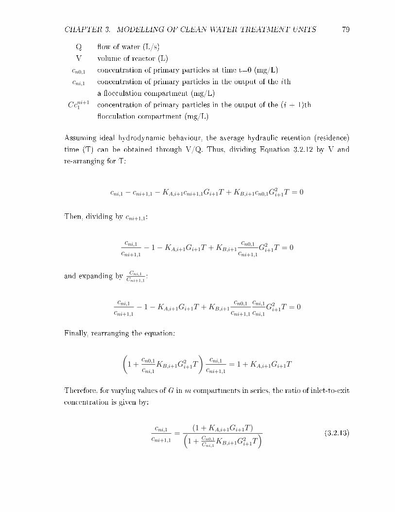
CHAPTER 3. MODELLING OF CLEAN WATER TREATMENT UNITS 79
Q �ow of water (L/s)
V volume of reactor (L)
cn0,1 concentration of primary particles at time t=0 (mg/L)
cni,1 concentration of primary particles in the output of the ith
a �occulation compartment (mg/L)
Ccni+11 concentration of primary particles in the output of the (i + 1)th
�occulation compartment (mg/L)
Assuming ideal hydrodynamic behaviour, the average hydraulic retention (residence)
time (T) can be obtained through V/Q. Thus, dividing Equation 3.2.12 by V and
re-arranging for T:
cni,1 − cni+1,1 −KA,i+1cni+1,1Gi+1T +KB,i+1cn0,1G2i+1T = 0
Then, dividing by cni+1,1:
cni,1cni+1,1
− 1−KA,i+1Gi+1T +KB,i+1cn0,1
cni+1,1
G2i+1T = 0
and expanding byCni,1Cni+1,1
:
cni,1cni+1,1
− 1−KA,i+1Gi+1T +KB,i+1cn0,1
cni+1,1
cni,1cni,1
G2i+1T = 0
Finally, rearranging the equation:
(1 +
cn0,1
cni,1KB,i+1G
2i+1T
)cni,1cni+1,1
= 1 +KA,i+1Gi+1T
Therefore, for varying values of G in m compartments in series, the ratio of inlet-to-exit
concentration is given by:
cni,1cni+1,1
=(1 +KA,i+1Gi+1T )(
1 + Cn0,1Cni,1
KB,i+1G2i+1T
) (3.2.13)
CHAPTER 3. MODELLING OF CLEAN WATER TREATMENT UNITS 80
and the overall change in concentration in the whole series of m compartments with
equal average velocity gradients, G, incorporating the relation average hydraulic reten-
tion (residence) time multiplied by the number of �occulation chambers, (T ·m), which
expresses the value responding to the total hydraulic retention (residence) time1 (τ)
can be written as (Argaman and Kaufman, 1970):
cn0,1
cnm,1=
(1 +KAG
τm
)m1 +KBG2 τ
m
∑m−1i=0
(1 +KAG
τm
)i (3.2.14)
The main limitation with using these models is that the derived expression assumes
that the �oc suspension is of constant size distribution so using a plug �ow reactor is
not applicable as the �oc size distribution will not be constant with time.
3.2.3 Numerical simulation and validation
In this section, the two �occulation models derived above will be simulated in gPROMS.
First, the models will be validated against the literature and then the limitations of the
models will be tested through a sensitivity analysis.
Model Parameters
Argaman (1971) conducted pilot-plant experiments in a �occulator to determine the
parameters which will be used in this work for model validation. The experiments
were conducted on an operating water treatment plant. Argaman (1971) interprets the
experimental results by using theoretical results of �occulation kinetics in turbulent
�uid. The experimental results (which can be found in Appendix B) are determined
from the values for KA and KB. All the parameter values can be found in Table 3.1.
Model validation and sensitivity analysis
The experimental and theoretical values determined by Argaman (1971) are compared
(in Table 3.2) with the predicted values calculated using the �oc formation in rapid
1Total hydraulic retention (residence) time is a measure of the average length of time that acompound (water) remains in a unit (�occulation chamber).

CHAPTER 3. MODELLING OF CLEAN WATER TREATMENT UNITS 81
Table 3.1: Model parameters for coagulation and �occulation model veri�cation(Argaman, 1971).
Description Parameters Value
Collision constant (-) KA 1.8 x 10⁻⁵
Break-up constant (s) KB 0.8 x 10⁻⁷
Total hydraulic retention (residence) time (s) τ 1800
Number of �occulation reactors (-) m 4
Velocity Gradient (s−1) G 20
Initial primary particle concentration (mg/L) cn0 10
Volumetric �owrate (L/s)* Q 0.44
*Based on a symmetrical basin with volume 52,000 gal, the area is approximately 36m2. This can be
used to estimate the velocity.
Table 3.2: Actual and predicted performance of a multi-compartment �occulator(Argaman, 1971).
Values ofcn01
cnm1
Number of
compartments,
i
Floc formation
in rapid mixing
(This work)
Floc formation in a
�occulation
chamber (This
work)
Simulated in
literature
(Argaman,
1971)
Prototype actual
performance
(Argaman, 1971)
1 - 1.15 1.15 1.08
2 - 1.33 1.32 1.18
3 - 1.55 1.48 1.45
4 1.78 1.80 1.73 1.75
mixing (Equations 3.2.10 and 3.2.11) and �oc formation in a �occulation chamber
model (Equations 3.2.13 to 3.2.14).
From the results, it can be seen that there is consistently good agreement between the
models developed in this work and literature. This suggests that these two models can
be used to represent the phenomena occurring in the coagulation and �occulation units.
To test the limitations of the models, sensitivity analysis will be conducted to:
1. Test the relationship between the velocity gradient and hydraulic residence time
in the �oc formation in �occulation chambers
2. Test how the �oc formation by rapid mixing reacts to a set of illustrative case
studies
These two sensitivity analyses are relevant to actual water treatment plants because
the amount of time a colloidal/primary particle spends in a �occulation chamber or is

CHAPTER 3. MODELLING OF CLEAN WATER TREATMENT UNITS 82
rapidly mixed will have an a�ect on the suspended solids concentration. Floc formation
can be hindered if the velocity gradient is too high promoting �oc break up in the e�uent
stream.
Sensitivity study 1: Floc formation in a �occulation chamber
Figure 3.3 shows the relationship between the velocity gradient, G, and the total
hydraulic retention (residence) time, τ , for the two examined case studies (�occulation
chamber with one and four compartments, respectively) for two di�erent values of
collision constant, KA and break-up constant, KB. It can be seen that for any desired
�occulation performance, there is a minimum retention (residence) time, below which
the performance can not be determined regardless of the velocity gradient. This
observation agrees well with those found in the literature where it is stated that the
product G · τ in itself is not an adequate parameter for describing the e�ects of stirring
energy and residence time on �occulation performance (Argaman, 1971; Crittenden
et al., 2012).
Both �gures illustrate the e�ect of compartmentalisation, particularly when the high
performance is desired. Figure 3.3a shows that for 75% removal of primary particles
(cn01 /cnm1 = 4), the total hydraulic retention (residence) time (ca. 700 s) required in a
four-compartment reactor is approximately half of the required time (ca. 2000 s) for
a single-compartment reactor. This is in contrast to what is observed in Figure 3.3b,
where the graph shows that for 75% removal (cn01 /cnm1 = 4), the single-compartment
reactor has a smaller retention (residence) time (ca. 13000 s) than a four-compartment
reactor (ca. 48000 s). This observation can be attributed to the smaller break-up
constant, KB, as for low velocity gradients, G, or for strong �ocs (with a small breakup
constant), the denominator of the equation 3.2.14 approaches unity; therefore increase
in the number of compartments would have no added e�ect on e�ciency but would be
detrimental to the process, as if KB<KA , the process will be dominated by kinetics
and this will promote �oc break up.
Sensitivity study 2: Floc formation in a rapid mixing unit
Figure 3.4 shows the relationship between primary particles forming suspended solid
particles (�ocs) and how the system would react to changes. The two case studies
implemented here are: (1) an initial 10% increase in the primary particle concentration
(in reality, this could be due to an increase in �owrate from an additional water source)
and (2) a 20% decrease in the impeller speed or velocity gradient (which could occur
when there is a need to promote aggregation in the system).

CHAPTER 3. MODELLING OF CLEAN WATER TREATMENT UNITS 83
Figure 3.3: Sensitivity analysis: Relationship between the velocity gradient, G, and thetotal hydraulic retention (residence) time, τ , for two di�erent case studies (�occulationchamber with one and four compartments, respectively) for two di�erent values ofcollision constant, KA and break-up constant, KB.a) Collision constant KA = 5.1× 10⁻⁵ and break-up constant KB = 1.1× 10⁻⁷
b) Smaller collision constant KA = 1.8× 10⁻⁵ and break-up constant KB = 0.8× 10⁻⁷.

CHAPTER 3. MODELLING OF CLEAN WATER TREATMENT UNITS 84
Figure 3.4: Sensitivity analysis: Relationship between primary particles formingsuspended particles (�ocs) in a rapid mixing unit and how the system would reactto speci�c changes. Two disturbances are implemented (black dotted line): 1) 10%increase in the primary particle concentration, and 2) 20% decrease in the impellerspeed or velocity gradient.
From Figure 3.4, it can be seen that following the �rst disturbance, with an increase of
primary particles to 0.97 mg/L, the system responds by �nding a new suspended solids
steady state at a lower concentration (0.43 mg/L). This is because collision and break
up parameters, KA and KB respectively, have not changed as they are considered to be
in equilibrium and the unit is now operating under its initial removal e�ciency. The
system is then restored to its original steady state, before another disturbance of 20%
decrease in the velocity gradient is introduced.
Figure 3.4 shows a steep increase in the formation and concentration of �ocs (suspended
solids) with the step decrease in velocity gradient. This is expected as slow mixing
promotes the aggregation of particles. As discussed in the previous sensitivity analysis,
a higher number of suspended solids would be formed from the collision of primary
particles with a low velocity gradient and small break up constant, which is in good
agreement with the literature (Argaman, 1971; Rietveld et al., 2009) and shows the
model is responding to system changes appropriately.
CHAPTER 3. MODELLING OF CLEAN WATER TREATMENT UNITS 85
3.2.4 Concluding remarks
The primary objective of the current study was to investigate the formation of �ocs
from primary particles and the relationship between the break up of �ocs back into
primary particles. Numerous �occulation models have been developed in the literature
originating from Smoluchowski's equation.
The mathematical model derived in Section 3.2.2 was used to simulate the Argaman
- Kaufman �occulation model; although data available for model validation is limited,
it can be said that the �ndings revealed that the model was in good agreement with
the existing data; however, relies heavily on an empirical relationship to estimate the
parameters needed. When comparing the simulated result with the data provided in
literature, it is clear that the trends are similar. In order to accurately predict the
performance of a full-scale water treatment plant, an experimental study should be
carried out to determine the actual values of the collision and break up constant KA
and KB to re�ect the same suspension and chemical expected in the treatment process.
3.3 Modelling of clari�cation process
In this section, a mathematical model based on sedimentation clari�cation is proposed
to represent the clean water clari�cation process. In addition, there is a discussion as to
why dissolved air �otation will not be modelled in this work. The mathematical model
proposes to simulate �oc (suspended solids) concentration and height of sludge blanket
within the sedimentation tank in time and space.
Dissolved air �otation
Dissolved air �otation is a commonly used clari�cation process; most models created to
represent the phenomena are developed through Computational Fluid Dynamic (CFD)
modelling, as obtaining an accurate predictive one-dimensional model of the process
unit is quite complex due to the presence of a large number of empirical parameters
such as particle-bubble attachment e�ciency, air-to-solids volume ratio, bubble volume
concentration etc. One-dimensional models that currently exist in the literature are able
to successfully show the bubble-�lter e�ciency in the contact zone and the removal
e�ciency in the separation zone both as products of residence time with empirical

CHAPTER 3. MODELLING OF CLEAN WATER TREATMENT UNITS 86
parameter inputs (more details can be found in the work of Bloom and Heindel (2003)).
The empirical parameters rely heavily on experimental data for predictions meaning the
models developed work on a case-by-case basis. As the aim of this work is to produce
predictive mathematical models, currently detailed modelling of dissolved air �otation
would be out of the scope.
3.3.1 Unit principle
The clari�cation unit is important as it ensures the �lters can be operated more easily
and cost-e�ectively to produce quality water. Sedimentation is a solid-liquid separation
process in which particles settle under the force of gravity and the clear water rises to
the top of the tank to be removed with the e�uent �ow. This process has been widely
used in water treatment to remove �ocs, inorganic and turbidity-causing particles.
3.3.2 Model development
The model developed represents the increase in suspended solids concentration within
the clari�cation unit. For simplicity purposes, the two main variables being considered
are the time and the convective settling function.
Model development of sedimentation clari�cation unit
As mentioned in Chapter 2, the mathematical modelling of conventional clean water
treatment units can also bene�t from various models developed to simulate wastewater
treatment process units as the wastewater industry is more advanced in mathematical
modelling of their processes. Due to the similarities in the phenomena occurring in a
secondary settling tank (SST) utilised in the activated sludge process2, this will be used
to describe the sedimentation clari�cation unit in clean water treatment. This section
will present a one-dimensional model to predict e�uent solids concentration in addition
to the sludge blanket height in the secondary settling tank (SST).
Figure 3.5 shows the schematic impression of an ideal SST. Generally, this unit can
be divided into three distinct zones according to their key functions: Clari�cation
2Activated sludge process is utilised in the wastewater treatment that has a post treatmentclari�cation unit.
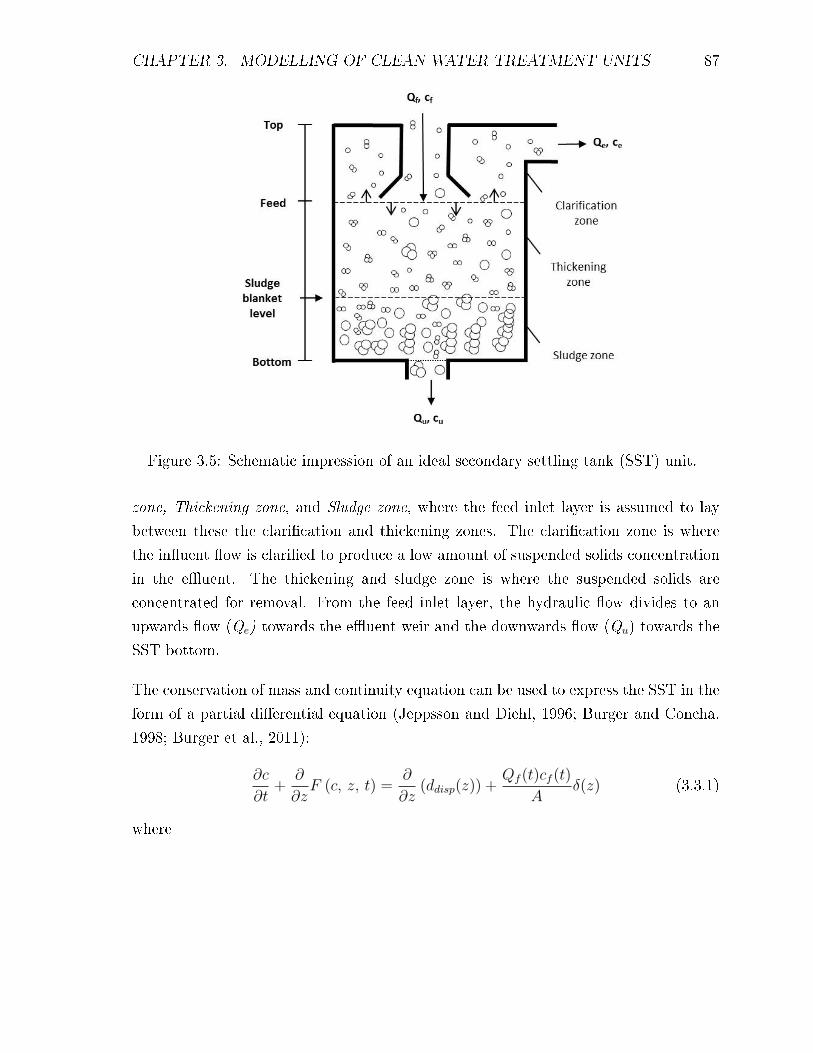
CHAPTER 3. MODELLING OF CLEAN WATER TREATMENT UNITS 87
Figure 3.5: Schematic impression of an ideal secondary settling tank (SST) unit.
zone, Thickening zone, and Sludge zone, where the feed inlet layer is assumed to lay
between these the clari�cation and thickening zones. The clari�cation zone is where
the in�uent �ow is clari�ed to produce a low amount of suspended solids concentration
in the e�uent. The thickening and sludge zone is where the suspended solids are
concentrated for removal. From the feed inlet layer, the hydraulic �ow divides to an
upwards �ow (Qe) towards the e�uent weir and the downwards �ow (Qu) towards the
SST bottom.
The conservation of mass and continuity equation can be used to express the SST in the
form of a partial di�erential equation (Jeppsson and Diehl, 1996; Burger and Concha,
1998; Burger et al., 2011):
∂c
∂t+
∂
∂zF (c, z, t) =
∂
∂z(ddisp(z)) +
Qf (t)cf (t)
Aδ(z) (3.3.1)
where

CHAPTER 3. MODELLING OF CLEAN WATER TREATMENT UNITS 88
c concentration (mg/L)
F (convective) �ux function (mg/m2s)
ddisp dispersion function (m2/s)
Q volumetric �ow rate (L/s)
A cross-sectional area of SST (m2)
z depth (m)
f subscript for inlet feed
The �rst term on the left hand side is the change of concentration with time. The
second term on the left-hand side models hindered settling3 combined with bulk �ows
that separate due to feed, under�ow and over�ow operations. The third term models
dispersion, and the �nal term is a singular source term which models the feed mech-
anism. The model presented here is a convection-dispersion model where the e�ects of
compression are not incorporated into the model as it is an added complexity which
provides little reward once the surrogate models are developed (Burger et al., 2012).
There are a variety of other assumptions made in the model development:
1. The particles concentration is uniform in the horizontal direction. It is therefore
a one-dimensional model (in the vertical z-direction).
2. The liquid and solid phases are incompressible, meaning there is no mass transfer
between them as the water is being clari�ed by removal of fully formed suspended
solid particles.
3. The particles are of similar sizes and shapes. This assumption is to simplify the
model as there is much discussion on the actual fractal shape of suspended solid
particles (Jarvis et al., 2005).
4. The velocity of sedimentation depends only on the local particle concentration
(this is a restrictive assumption as it does not account for the population of
suspended solid particles).
5. The velocity tends to zero as suspended solids concentration, c, tends to a max-
imum value cmax as the solids have reached the top of the sludge blanket indicating
the end of settling.
3Within hindered settling, the mass of particles will settle as a unit with individual particlesremaining in �xed positions with respect to each other. Zones of di�erent concentrations may developfrom segregation of particles with di�erent settling velocities.

CHAPTER 3. MODELLING OF CLEAN WATER TREATMENT UNITS 89
With the unit area being constant, and taking into account the the two volumetric
upward and downward �ows and hindered settling velocity within the SST:
F (c, z, t) =
−Qe(z)c/A for z < Top
fbk(c) −Qe(z)c/A for Top < z < 0
fbk(c) −Qe(z)c/A+Qu(z)c/A for z = 0
fbk(c) +Qu(z)c/A for 0 < z < Bottom
+Qu(z)c/A for z > Bottom
(3.3.2)
where the convective �ux function involves the Kynch batch density function (Kynch,
1952), fbk:
fbk = c.vhs (3.3.3)
The hindered settling velocity vhs(c) is a function of concentration only (Kynch, 1952):
vhs(c) = v0e−rc (3.3.4)
f bk(c) = v0ce−rc (3.3.5)
where
Top height of clari�cation zone (m)
Bottom depth of thickening zone (m)
fbk Kynch batch �ux density function (mg/(m2s))
vhs hindered settling velocity (m/s)
v0 settling velocity of a single particle in unbounded �uid (m/s)
r parameter in equation 3.3.5 (L/mg)
The dispersion function, ddisp, is often set as a product of the �uid velocity and a
continuous function (Burger et al., 2011):
ddisp(z) =
α1Qf · exp(−z2/(α2Qf)
2
1−|z|/(α2Qf)
)for |z| < α2Qf
0 for |z| ≥ α2Qf
(3.3.6)
where the parameters α1 and α2 are greater than zero. One of the idealising assumptions
is that the suspended solids/water mixture follows the bulk �ows in the outlet pipes.

CHAPTER 3. MODELLING OF CLEAN WATER TREATMENT UNITS 90
Table 3.3: Parameters to be implemented into gPROMS for the clari�cation unit(Burger et al., 2012).
Description Parameter ValueHeight of clari�cation zone (m) Top -1Depth of thickening zone (m) Bottom 3Cross-sectional area (m2) A 400
Maximum concentration (mg/L) cmax 20×103
Settling velocity of a single particle in unbounded �uid (m/s) v0 3.47Parameter in equation for fbk (L/mg) r 0.37×10⁻³
Parameter in dispersion coe�cient (m−1) α1 2.3×10⁻³
Parameter in dispersion coe�cient (h/m2) α2 2.5×10⁻³
Concentration at feed inlet (mg/L) cmhn f 4.5×10³
Feed volumetric �owrate (L/h) Qf 230×103
Under�ow volumetric �owrate (L/h) Qu 100×103
This means that as the suspended solids/water mixture leaves the SST, it cannot return
(Burger et al., 2011); thus suggesting:
ddisp(z)
= 0 for z ≤ Top and z ≥ Bottom
≥ 0 for Top < z < Bottom(3.3.7)
3.3.3 Model simulation and validation
In this section, the clari�cation model derived above will be simulated in gPROMS.
Various assumptions were made in the development of this model. The simulation
results produced from this model are evaluated in the following section. First, the
models will be validated against literature and then the limitations of the models will
be tested through a sensitivity analysis.
Model parameters
Burger et al. (2012) tested their convection-dispersion-compression model with para-
meters that will currently be used for model validation. Table 3.3 shows the values of
the model parameters for the simulation.

CHAPTER 3. MODELLING OF CLEAN WATER TREATMENT UNITS 91
Model validation and sensitivity analysis
In solving the equations, as a function of time and height solution discontinuities are
expected to occur. This can be interpreted physically as the sediment interface or
sludge blanket height that can also be observed in experiments (Li and Stenstrom,
2014). The use of the Godunov approach was initially proposed by Jeppsson and Diehl
(1996); in this approach, the concentration related to each grid point at a given time
point is calculated as the average of an analytical solution that originates from piecewise
constant initial data at the preceding time point. The details of how this is implemented
to simulate this model can be found in Appendix C.
The literature case study simulated to validate the model in this work can be in found
Figures 3.6a and 3.6b. The simulation begins at steady state for the �rst 5 hours and
then a step increase is imposed on the feed volumetric �owrate changing the value to
360×103 L/hr, the feed concentration is decreased by 10% and the under�ow volumetric
�owrate is kept constant. This change is kept for 15 hours after which all variables are
returned to steady state. Burger et al. (2012) incorporates compression into their model
which has an a�ect on the second step change imposed on the system. In Figures 3.6a
and 3.6b, there is a gradual decreases in concentration to steady state between t = 20
hrs to t = 48 hrs. This is, however, not observed in Figure 3.6c as the model in Figures
3.6a and 3.6b incorporates compression conditions into the system.
Between t = 0 hr to t = 20 hrs, Figure 3.6c shows a trend to represent the formation of
a sludge blanket; this is formed approximately one metre from the bottom of the tank
and there is an increase in solids concentration the closer to the bottom of the tank as
the suspended solids start to settle there. However, with the omission of the sediment
compression function, the dynamic simulation results for the gPROMS clari�er model
presented here and from Burger et al. (2012) are in good agreement, as the model is
still able to represent the phenomena occurring in the sedimentation clari�cation unit.
To test the limitations of the model, a sensitivity analysis is conducted to check the
robustness of the model with regards to the number of discretised points. As the sludge
blanket is formed with discontinuous behaviour, this would mean that the discretisation
model and detail will have an a�ect on the overall representation of the model.
Sensitivity study: E�ect of layer number on the system
The simulations are performed for three di�erent cases with 10, 20 and 30 grid points/layers
using the same parameters presented in Table 3.3. Figure 3.7 shows that the predictions

CHAPTER 3. MODELLING OF CLEAN WATER TREATMENT UNITS 92
Figure 3.6: A dynamic simulation of the convection-di�usion clari�ermodel starting at steady state with the parameters found in Table 3.3.a) literature simulation with 10 discretised points (Burger et al., 2012).b) literature reference simulation, both are reproduced from literature with permission(Burger et al., 2012).c) simulation using the model shown in Equation 3.3.1 with 10 discretised points.

CHAPTER 3. MODELLING OF CLEAN WATER TREATMENT UNITS 93
Figure 3.7: A steady state simulation of the sedimentation clari�cation unit using theparameters in Table 3.3. The concentration pro�le of di�erent discretisation levels: 10,20 and 30 are shown.
diverge with di�erences in the sludge blanket level and the under�ow concentration.
Except for the case of 10 layers, the di�erence between the concentrations calculated
with the other layers is not too large. This shows that 10 layers is clearly not enough
to accurately predict the suspended solids concentration as it underpredicts the con-
centration within the thickening zone.
3.3.4 Concluding remarks
The primary objective of modelling a one-dimensional sedimentation clari�cation unit
was to investigate the suspended solid settling characteristics, such as suspended solids
concentration and height of sludge blanket formed at the bottom of the unit. Most
of the focus in this section has been placed on a sedimentation clari�cation unit as
the development of a predictive model can be obtained. Dissolved air �otation is
another commonly used clari�cation unit; however, obtaining an accurate predictive
one dimensional model of the process unit is quite complex due to the presence of a
large number of empirical parameters. Developing a detailed model of dissolved air
�otation is out of the scope for this work.

CHAPTER 3. MODELLING OF CLEAN WATER TREATMENT UNITS 94
The mathematical model developed in Section 3.3.2 was used to simulate suspended
solids concentration within the clari�cation unit. The limitations and sensitivity of
the model were tested to see what could be improved. The comparison in Figure
3.6 demonstrates a reasonable agreement between literature results and the simulated
gPROMS clari�cation model developed in this work. It can be concluded from this
preliminary study that this model is capable of predicting the sludge blanket height and
settling time to an acceptable degree but further work, such as around the compression
function, would be needed to make it more robust.
3.4 Modelling of �ltration
In this section, a model is being proposed to simulate a two-stage hypothesis of the
phenomena occurring within the rapid gravity �ltration process. This model considers
the attachment and detachment of suspended particle deposits onto a porous medium.
3.4.1 Unit principle
The purpose of �ltration is the removal of solid particles from the water by passing the
solid/water mixture through a porous medium or other suitable material to capture the
solid particles whilst allowing the water to pass through, thus achieving the required
quality of �ltered water. This unit is usually the third physical unit in the clean water
treatment process and is often the last line of defense to removal �oc and colloidal
particles from entering the water distribution by their retention in the porous medium.
A porous medium is a solid matrix containing voids which interconnect to enable the
�uid �ow through the medium at a low speed. The media thereby retains most of the
solid matter within the pore structure.
3.4.2 Model development
As explained in Chapter 2, mathematical modelling of �ltration can be divided into
two sub-categories: macroscopic (deals with the cumulative collection of deposits)
and microscopic (considers the size of the individual particle as well as the number
of particles).
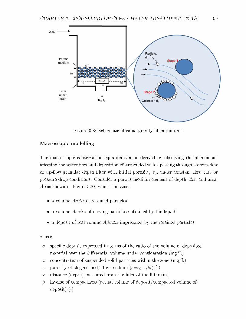
CHAPTER 3. MODELLING OF CLEAN WATER TREATMENT UNITS 95
Figure 3.8: Schematic of rapid gravity �ltration unit.
Macroscopic modelling
The macroscopic conservation equation can be derived by observing the phenomena
a�ecting the water �ow and deposition of suspended solids passing through a down-�ow
or up-�ow granular depth �lter with initial porosity, ε0, under constant �ow rate or
pressure drop conditions. Consider a porous medium element of depth, ∆z, and area,
A (as shown in Figure 3.8), which contains:
� a volume Aσ∆z of retained particles
� a volume Aεc∆z of moving particles entrained by the liquid
� a deposit of real volume Aβσ∆z imprisoned by the retained particles
where
σ speci�c deposit expressed in terms of the ratio of the volume of deposited
material over the di�erential volume under consideration (mg/L)
c concentration of suspended solid particles within the zone (mg/L)
ε porosity of clogged bed/�lter medium (ε=ε0 - βσ) (-)
z distance (depth) measured from the inlet of the �lter (m)
β inverse of compactness (actual volume of deposit/compacted volume of
deposit) (-)

CHAPTER 3. MODELLING OF CLEAN WATER TREATMENT UNITS 96
Following the model created by Han et al. (2008), a two-stage hypothesis is a developed
to represent the entire rapid gravity �ltration process (as shown in Figure 3.8):
Stage 1: Suspended solid particles begin depositing outside of the �lter grains. The
particles that deposited previously start to serve as additional collector sites to enhance
further attachment of suspended particles. During this time period, detachment of
deposited particles does not occur until the speci�c deposit reaches a critical speci�c
deposit, σc. This assumption is consistent with experiments carried out by Ison and
Ives (1969). The authors demonstrate over several hours of �ltration, the experiments
show that clay deposits accumulated onto the grain, and were then partially detached
by arrival of further suspended particles. Thus, proving that detachment of particles
during �ltration is an occurring phenomenon when substantial amounts of deposit are
present.
Stage 2: During this stage detachment starts to occur. This is due mainly an increase
of the hydraulic shear forces with an increased interstitial velocity within the free space
of the �lter media. At the second stage, both deposition and detachment occurs.
The general material balance of particles can be written as:
accumulation rate = (flow in) − (flow out)
or∂ [A (σ + εc)]
∂t+∂(Auc− ADz
∂c∂z
)∂z
= 0 (3.4.1)
where
Aσ volume of particles retained in a unit depth �lter (m2.mg/L)
Aεc volume of particles in motion entrained by liquid in a unit depth �lter
(m2.mg/L)
Auc particle �ow entrained by the �uid (mg/s)
Dz dispersion coe�cient in water (m2/s)
-ADz (∂c/∂z) di�usional �ux of particles (m4/s)
ε0 clean bed porosity (-)
The assumptions used when deriving the model are:
� Axial dispersion is assumed negligible which is true for small particle sizes.
� Filtration takes place throughout the entire �lter and no macroscopic transverse
mass or �ow variations take place within the zone under consideration.

CHAPTER 3. MODELLING OF CLEAN WATER TREATMENT UNITS 97
� The velocity of suspension is constant throughout the �lter.
Under these assumptions, the material balance of particles in a di�erential volume of
the �lter is written as:
(∂ (σ + εc)
∂t
)z
+ vs
(∂c
∂z
)t
= 0 (3.4.2)
where vs is the �ltration velocity and ε is the porosity of the �lter media. The porosity
of the �lter, ε, varies with time and with the speci�c deposit due to particle deposition
on grain surfaces, altering the morphology of the void space of the porous medium
(Skouras et al., 2011). This variation can be expressed as:
ε = ε0 −σ
1− εd(3.4.3)
where εd is the porosity of the deposits. At early stages of �ltration, the porosity is
nearly constant, and Equations 3.4.2 and 3.4.3 can be rewritten as:
vs∂c
∂z+ ε0
∂c
∂t+∂σ
∂t= 0 (3.4.4)
For a homogeneous �lter, ε0 is constant, and τf can be estimated from the expression
(Skouras et al., 2011):
τf = t− ε0z
u(3.4.5)
where τf is the time elapsed before a given amount of the suspended solids reaches the
depth z. The di�erence between t and τf is usually negligible (Han et al., 2008). Then,
Equation 3.4.4 can be written as:
u∂c
∂z+∂σ
∂t= 0 (3.4.6)
The rate of particle deposition can be written in terms of the speci�c deposit, σ, or the
particle concentration, c. The basic granular �ltration equation proposed in 1937 by
Iwaki, which was later experimentally veri�ed by Ison and Ives (1969), is as follows:
− ∂c
∂z= λc (3.4.7)
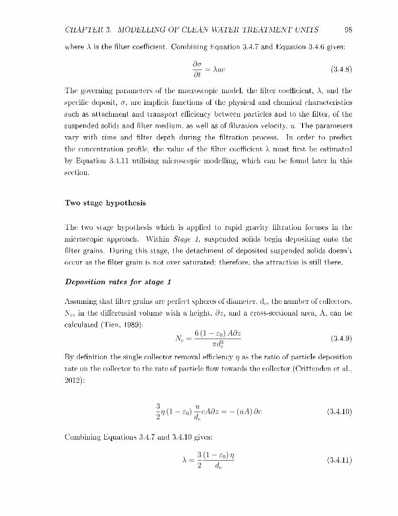
CHAPTER 3. MODELLING OF CLEAN WATER TREATMENT UNITS 98
where λ is the �lter coe�cient. Combining Equation 3.4.7 and Equation 3.4.6 gives:
∂σ
∂t= λuc (3.4.8)
The governing parameters of the macroscopic model, the �lter coe�cient, λ, and the
speci�c deposit, σ, are implicit functions of the physical and chemical characteristics
such as attachment and transport e�ciency between particles and to the �lter, of the
suspended solids and �lter medium, as well as of �ltration velocity, u. The parameters
vary with time and �lter depth during the �ltration process. In order to predict
the concentration pro�le, the value of the �lter coe�cient λ must �rst be estimated
by Equation 3.4.11 utilising microscopic modelling, which can be found later in this
section.
Two stage hypothesis
The two stage hypothesis which is applied to rapid gravity �ltration focuses in the
microscopic approach. Within Stage 1, suspended solids begin depositing onto the
�lter grains. During this stage, the detachment of deposited suspended solids doesn't
occur as the �lter grain is not over saturated; therefore, the attraction is still there.
Deposition rates for stage 1
Assuming that �lter grains are perfect spheres of diameter, dc, the number of collectors,
Nc, in the di�erential volume with a height, ∂z, and a cross-sectional area, A, can be
calculated (Tien, 1989):
Nc =6 (1− ε0)A∂z
πd3c
(3.4.9)
By de�nition the single collector removal e�ciency η as the ratio of particle deposition
rate on the collector to the rate of particle �ow towards the collector (Crittenden et al.,
2012):
3
2η (1− ε0)
u
dccA∂z = − (uA) ∂c (3.4.10)
Combining Equations 3.4.7 and 3.4.10 gives:
λ =3
2
(1− ε0) η
dc(3.4.11)

CHAPTER 3. MODELLING OF CLEAN WATER TREATMENT UNITS 99
O'Melia and Ali (1978) suggested during the ripening stage, the actual collector consists
of a �lter grain and an associated number of particles deposited on it that also serve
as collectors, and the removal e�ciency of the single collector was calculated by (Han
et al., 2008):
η = αη0 +Nαpηp
(dpdc
)2
(3.4.12)
and
N = αη0β
(3
2x (1000 × ρp)
d2c
d3p
)u
ˆ t
0
c∂t (3.4.13)
where
η single collector removal e�ciency (-)
η0 single collector contact e�ciency in the clean �lter bed (-)
ηp single deposited particle contact e�ciency (-)
α particle/�lter grain attachment coe�cients (-)
αp particle/particle attachment coe�cients (-)
β factor of particles deposited directly onto the �lter grain which can act as
additional collectors (-)
ρp suspended solid density (mg/L)
dc collector diameter (m)
dp particle diameter (m)
N number of deposited particles per �lter grain which acts as additional
collectors (-)
Obtaining particle/�lter grain transport e�ciency in the clean �lter
The particle/�lter grain transport e�ciency in the clean �lter, η0, can be calculated
from a correlation developed by Rajagopalan and Tien (1976):
η0 = 4A1/3s Pe
−2/3 + AsN1/8LON
15/8R + 3.38x 10⁻³AsN
1.2G N−0.4
R (3.4.14)
where
As =1 (1− p5)
w(3.4.15)
w = 2− 3p+ 3p5 − 2p6 (3.4.16)
p = (1− ε)1/3 (3.4.17)
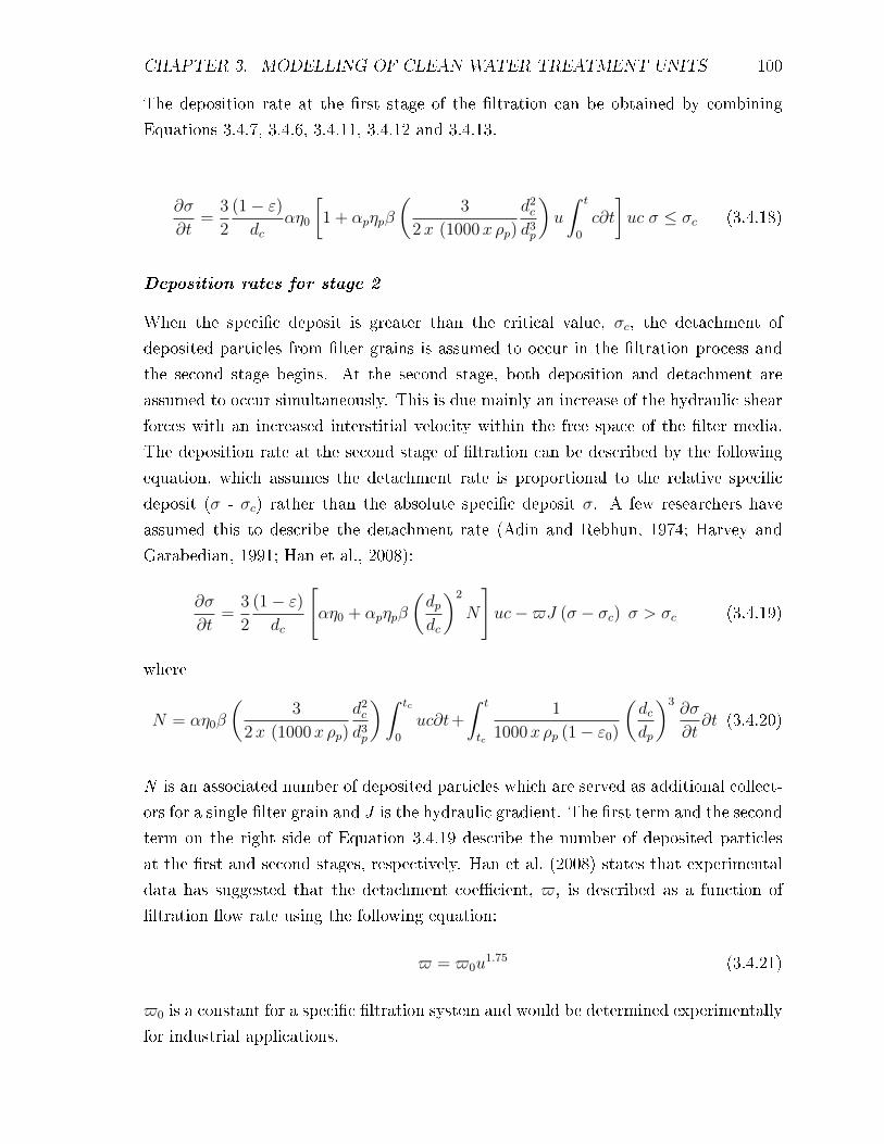
CHAPTER 3. MODELLING OF CLEAN WATER TREATMENT UNITS 100
The deposition rate at the �rst stage of the �ltration can be obtained by combining
Equations 3.4.7, 3.4.6, 3.4.11, 3.4.12 and 3.4.13.
∂σ
∂t=
3
2
(1− ε)dc
αη0
[1 + αpηpβ
(3
2x (1000x ρp)
d2c
d3p
)u
ˆ t
0
c∂t
]uc σ ≤ σc (3.4.18)
Deposition rates for stage 2
When the speci�c deposit is greater than the critical value, σc, the detachment of
deposited particles from �lter grains is assumed to occur in the �ltration process and
the second stage begins. At the second stage, both deposition and detachment are
assumed to occur simultaneously. This is due mainly an increase of the hydraulic shear
forces with an increased interstitial velocity within the free space of the �lter media.
The deposition rate at the second stage of �ltration can be described by the following
equation, which assumes the detachment rate is proportional to the relative speci�c
deposit (σ - σc) rather than the absolute speci�c deposit σ. A few researchers have
assumed this to describe the detachment rate (Adin and Rebhun, 1974; Harvey and
Garabedian, 1991; Han et al., 2008):
∂σ
∂t=
3
2
(1− ε)dc
[αη0 + αpηpβ
(dpdc
)2
N
]uc−$J (σ − σc) σ > σc (3.4.19)
where
N = αη0β
(3
2x (1000x ρp)
d2c
d3p
) ˆ tc
0
uc∂t+
ˆ t
tc
1
1000x ρp (1− ε0)
(dcdp
)3∂σ
∂t∂t (3.4.20)
N is an associated number of deposited particles which are served as additional collect-
ors for a single �lter grain and J is the hydraulic gradient. The �rst term and the second
term on the right side of Equation 3.4.19 describe the number of deposited particles
at the �rst and second stages, respectively. Han et al. (2008) states that experimental
data has suggested that the detachment coe�cient, $, is described as a function of
�ltration �ow rate using the following equation:
$ = $0u1.75 (3.4.21)
$0 is a constant for a speci�c �ltration system and would be determined experimentally
for industrial applications.

CHAPTER 3. MODELLING OF CLEAN WATER TREATMENT UNITS 101
Headloss through the �lter column
Headloss in a �lter bed is an important factor for the �lter bed conditions, and can
be used as an indicator to start �lter washing. Assuming a constant �ltration �ow
rate u, the deposition of suspended solids σ, on the surface of a �lter media causes
clogging. This results in a reduction in permeability. O'Melia and Ali (1978) suggested
that permeability is inversely proportional to the square of the inter-facial surface area
in the �lter (Han et al., 2008). The hydraulic gradient within a clogged �lter can be
expressed as:
J = J0
(1 +
γ
ρpσ
)2
(3.4.22)
where γ is an empirical parameter which is relates the �ow rate, clean �lter bed porosity,
�lter grain size, and the particle surface area-to-volume ratio. From experimental data
in the literature (Yao et al., 1971), γ was proposed to be expressed as:
γ = γ0u−0.55 (3.4.23)
where γ0 is a constant for speci�c �ltration system. Combining Equation 3.4.22 and
Equation 3.4.23 gives:
J = J0
(1 +
γ0
ρpu−0.55σ
)2
(3.4.24)
Therefore, the headloss through the �lter can be calculated by:
h = J0
ˆ L
0
(1 +
γ0
ρpu−0.55σ
)2
∂z (3.4.25)
The hydraulic gradient in the clean �lter bed J0 can be experimentally obtained or
calculated by the Carmen-Kozany equation.
J0 =h0
L(3.4.26)
Initial and Boundary Conditions
For �ltration with a clean �lter, the initial conditions states that the concentration
along the space in the column, c(z) is equal to the inlet concentration cin and the
speci�c deposit, σ, onto the media is 0. The boundary condition states that for the
�ltration time, the concentration at the inlet height, c(z = 0) is equal to the initial
concentration,cin:
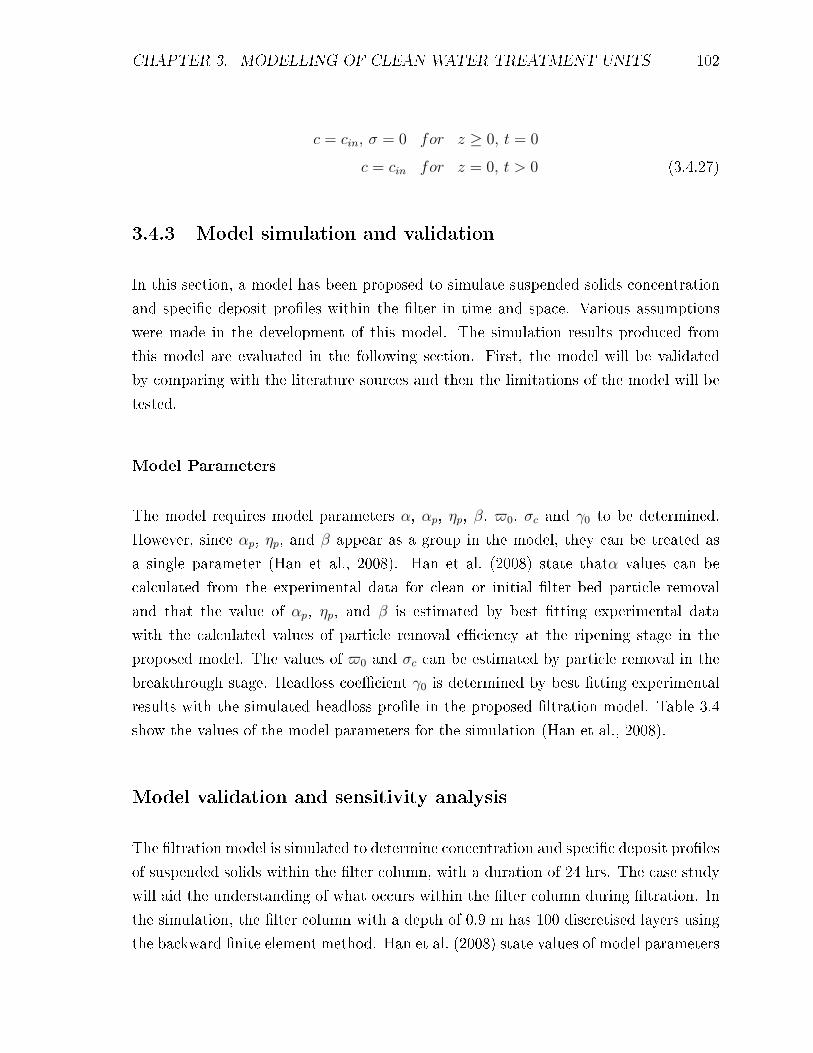
CHAPTER 3. MODELLING OF CLEAN WATER TREATMENT UNITS 102
c = cin, σ = 0 for z ≥ 0, t = 0
c = cin for z = 0, t > 0 (3.4.27)
3.4.3 Model simulation and validation
In this section, a model has been proposed to simulate suspended solids concentration
and speci�c deposit pro�les within the �lter in time and space. Various assumptions
were made in the development of this model. The simulation results produced from
this model are evaluated in the following section. First, the model will be validated
by comparing with the literature sources and then the limitations of the model will be
tested.
Model Parameters
The model requires model parameters α, αp, ηp, β, $0, σc and γ0 to be determined.
However, since αp, ηp, and β appear as a group in the model, they can be treated as
a single parameter (Han et al., 2008). Han et al. (2008) state thatα values can be
calculated from the experimental data for clean or initial �lter bed particle removal
and that the value of αp, ηp, and β is estimated by best �tting experimental data
with the calculated values of particle removal e�ciency at the ripening stage in the
proposed model. The values of $0 and σc can be estimated by particle removal in the
breakthrough stage. Headloss coe�cient γ0 is determined by best �tting experimental
results with the simulated headloss pro�le in the proposed �ltration model. Table 3.4
show the values of the model parameters for the simulation (Han et al., 2008).
Model validation and sensitivity analysis
The �ltration model is simulated to determine concentration and speci�c deposit pro�les
of suspended solids within the �lter column, with a duration of 24 hrs. The case study
will aid the understanding of what occurs within the �lter column during �ltration. In
the simulation, the �lter column with a depth of 0.9 m has 100 discretised layers using
the backward �nite element method. Han et al. (2008) state values of model parameters

CHAPTER 3. MODELLING OF CLEAN WATER TREATMENT UNITS 103
Table 3.4: Parameters to be implemented in gPROMS for the rapid gravity �ltrationunit (Han et al., 2008).
Description Parameters ValueFilter bed depth (m) L 0.9In-�uent particle concentration (mg/L) cin 6Super�cial velocity (m/h) u 5Clean grain diameter (m) dc 0.8 ×10⁻³
Particle diameter (m) dp 4 ×10⁻⁶
Porosity (-) ε0 0.4Particle/�lter grain attachment e�ciency (-) α 0.9Single parameter (-) αp, ηp, β 0.9Detachment coe�cient constant (-) $0 200Transitional speci�c deposit (mg/L) σc 300Particle density (mg/L) ρp 1350 x 103
Constant parameter (-) γ0 30Clean headloss (m) h0 0.4
that were intentionally chosen to make breakthrough4 take place signi�cantly, so that
the proposed �ltration model can be assessed.
Figure 3.9a (Han et al., 2008) and Figure 3.9b (this work) represent the changes in
suspended solids concentration with �ltration time at 3 di�erent positions in space
(z = 0.045 m, z = 0.45 m and z = 0.85 m). These positions are re�ective of the
top, middle and bottom of the tank respectively. The �gures show the suspended
solids concentration in the upper layer (z = 0.045 m) is high during �ltration and the
breakthrough stage occurs quickly. As we move down the �lter column, there is a delay
in occurrence of the breakthrough stage and the suspended particle concentrations in
the working stage continuously decreases. The model is able to be used to represent the
phenomena occurring in the �ltration unit due to a comparison between Figure 3.9a
and Figure 3.9b which shows they are in good agreement.
To test the limitations of the model, a sensitivity analysis is conducted to:
1. Test the relationship between e�uent suspended solids concentration and headloss
through the �lter column to con�rm the importance of headloss and to see if it can
be used as an indicator for back-wash within this model. This is informative for
purposes as it can aid in the identi�cation of in�uential parameters by quantifying
4Reminder: Breakthrough is the point at which the �lter grains are oversaturated with suspendedsolid deposits; thus the e�ciency decreases and suspended solids concentration increases as thesuspended solids detach from the grain.
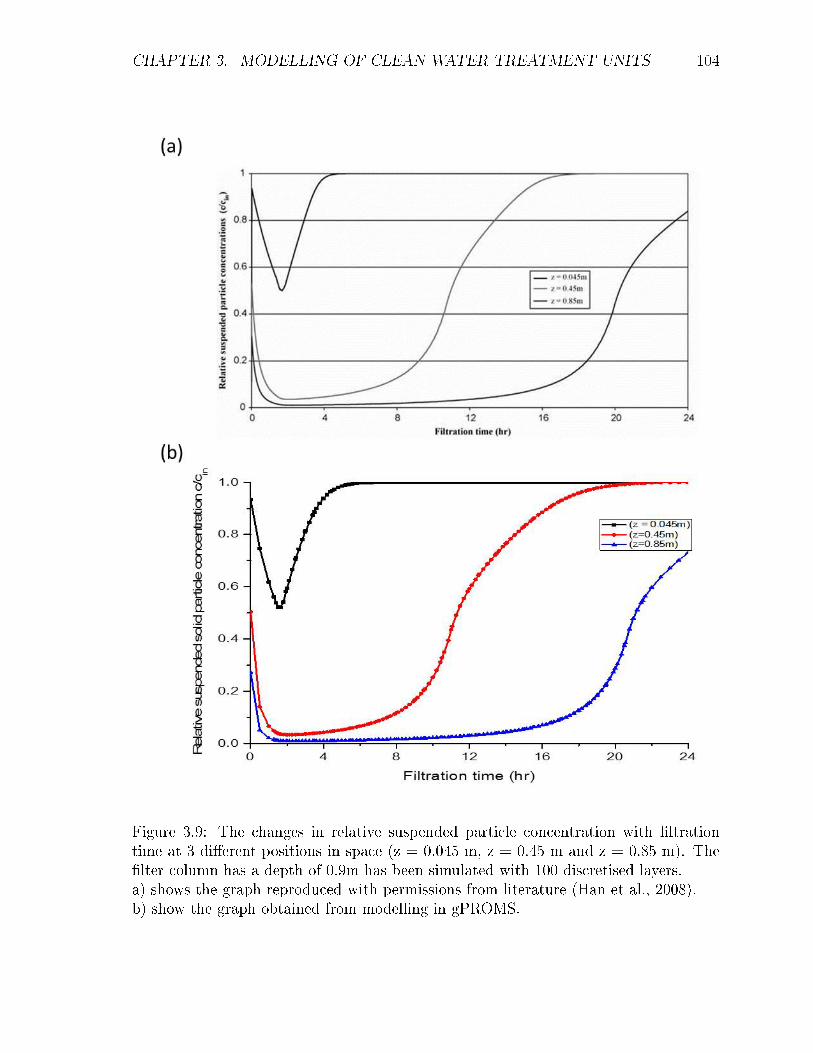
CHAPTER 3. MODELLING OF CLEAN WATER TREATMENT UNITS 104
Figure 3.9: The changes in relative suspended particle concentration with �ltrationtime at 3 di�erent positions in space (z = 0.045 m, z = 0.45 m and z = 0.85 m). The�lter column has a depth of 0.9m has been simulated with 100 discretised layers.a) shows the graph reproduced with permissions from literature (Han et al., 2008).b) show the graph obtained from modelling in gPROMS.
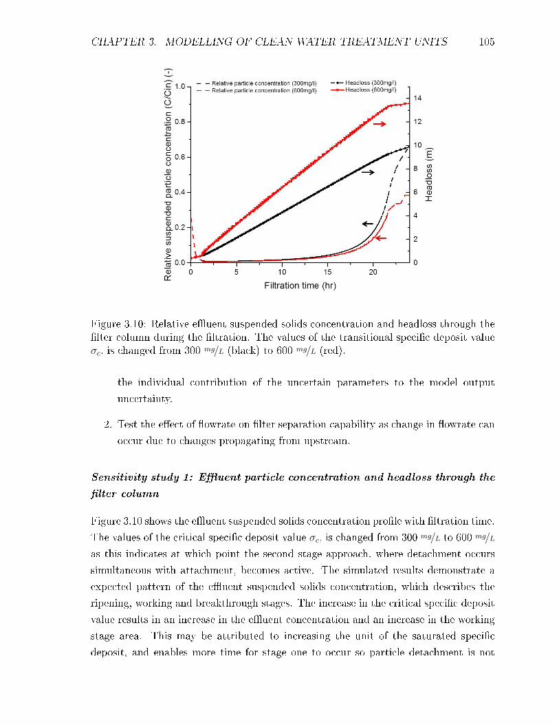
CHAPTER 3. MODELLING OF CLEAN WATER TREATMENT UNITS 105
Figure 3.10: Relative e�uent suspended solids concentration and headloss through the�lter column during the �ltration. The values of the transitional speci�c deposit valueσc, is changed from 300 mg/L (black) to 600 mg/L (red).
the individual contribution of the uncertain parameters to the model output
uncertainty.
2. Test the e�ect of �owrate on �lter separation capability as change in �owrate can
occur due to changes propagating from upstream.
Sensitivity study 1: E�uent particle concentration and headloss through the
�lter column
Figure 3.10 shows the e�uent suspended solids concentration pro�le with �ltration time.
The values of the critical speci�c deposit value σc, is changed from 300 mg/L to 600 mg/L
as this indicates at which point the second stage approach, where detachment occurs
simultaneous with attachment, becomes active. The simulated results demonstrate a
expected pattern of the e�uent suspended solids concentration, which describes the
ripening, working and breakthrough stages. The increase in the critical speci�c deposit
value results in an increase in the e�uent concentration and an increase in the working
stage area. This may be attributed to increasing the unit of the saturated speci�c
deposit, and enables more time for stage one to occur so particle detachment is not

CHAPTER 3. MODELLING OF CLEAN WATER TREATMENT UNITS 106
Figure 3.11: The e�ect of �ow rates (4 m/s, 5 m/s, 6 m/s and 7 m/s) on relative e�uentsuspended solids concentration.
taken into account at this stage. The estimated parameters for this model are important
features as varying them has an e�ect on the results. The �gure also shows headloss
through the �lter increases with �ltration time. The headloss of �lter media initially
increases and then starts to slow down over time, which is due to most of the �lter
has being saturated. This agreement can also be seen with the corresponding relative
suspended solids e�uent concentration showing the head loss would also be a good
indicator of back-washing time.
Sensitivity study: E�ect of �owrate on �lter separation capability
Four di�erent �ow rates (4 m/s, 5 m/s, 6 m/s and 7 m/s) were chosen to simulate
how suspended solids e�uent concentrations e�ect the ability to remove suspended
solids from water within the �lter. Figure 3.11 shows that the e�uent suspended solids
concentration signi�cantly increase with increase in �ow rate; this may be as a result of
the increase in �owrate enhancing the detachment of already deposited particles from
the �lter grains due to increased velocity, as described in the �ltration model. The
saturated speci�c deposit decreases with the increase in �ow rate, which agrees with
�ndings in literature.

CHAPTER 3. MODELLING OF CLEAN WATER TREATMENT UNITS 107
3.4.4 Concluding remarks
The primary objective of the this study was to investigate the particle removal behaviour
of �lters under realistic operating conditions and to simulate a model based on literature.
Numerous models to predict the removal e�ciency in deep bed �ltration at initial
and transient stages have been examined in the past (Rajagopalan and Tien, 1976).
However, research is still being conducted to develop a model that can describe the
entire �lter cycle to an excellent standard incorporating back-washing. The inclusion of
back-wash is out of the scope for this work; however, a detailed discussion is provided
in Chapter 6.
The mathematical model derived in Section 3.4.2 was used to simulate a two-stage
�ltration model developed by Han et al. (2008). An objective of this study was a
simulation of a �ltration model to test the limitations and to see what can be improved.
A comparison demonstrated a reasonable agreement between literature results and
the simulated gPROMS �ltration model. It can be concluded from this study that
this model is capable of predicting particle removal and headloss during rapid gravity
�ltration to a certain degree but further work, such as incorporating the back-washing
system into the model, is needed to make it more robust.
3.5 General discussion of model development
In this chapter, physical processes from clean water treatment works, namely co-
agulation/�occulation, clari�cation, and �ltration units, are simulated. The detailed
models are validated, where possible, with literature data before a sensitivity analysis
is conducted. Some are modelled with alternative methods of operation, such as rapid
mixing and �occulation in chambers for the coagulation/�occulation process.
Coagulation and �occulation models have been developed in literature originating from
Smoluchowski's equation which deals with the surface chemical e�ects in a simplistic
manner. This leads to a poor understanding of the interactions between the chemicals,
the coagulant dose and the primary particles, which leaves a scope for future work. The
models utilised in this study from the Argaman-Kaufman �occulation model, for both
a rapid mixing unit and a series of �occulation occurring in chambers, and the dissolved
air �otation model relies on empirical relationships to identify parameters needed.

CHAPTER 3. MODELLING OF CLEAN WATER TREATMENT UNITS 108
The model representing the sedimentation clari�cation unit was able to accurately
portray the phenomena predicted to occur within the unit in real life settings. The
main limitation with the model is neglecting a compression function which can add
another dimension to the model; however adding a compression function to the model
increases the computation complexity of the model for little reward, especially with the
creation of surrogate models, which will be discussed in a later chapter. This model
will be used for scenario analysis (especially the e�ect of an additional sludge settling
unit) and will play an important role in clean water treatment modelling. The inlet to
this unit is water from the under�ow outlet and enables the collection of water from
the sludge, which can be recycled to join the pipeline before entering the coagulation
and �occulation unit (simulations of these connected units can be seen in Chapter 4).
The �ltration model successfully simulated the three sub-stages occurring in �ltration
enabling an accurate representation of the phenomena occurring so for further improve-
ment the incorporation of a predictive back-wash model will strengthen the applicability
to a complete water treatment plant model.
One shortcoming with the models shown in this chapter is due to the fact they are
all modelled individually, �ideal� conditions are often assumed which will have an
e�ect on the predicted concentration, once the units have been combined to make
a complete clean water treatment model. Another shortcoming is that due to the
nature of the process models, empirical parameters are needed for accurate simulation
of a process on a speci�c site, which requires experiments or historical data to �nd
empirical relationships. However, this means there will be an indication of where to
explore experimentally and thus, provides useful information for innovation.
3.6 Conclusion
With drinking water standards becoming more rigorous, mathematical models will
become an important tool to assess clean water plant performance (Van Hulle et al.,
2006). Simulation is a useful tool and this chapter focuses on the use of numerical
simulation for the dynamic modelling of processes. One of the main problems with
the existing work on dynamic modelling water treatment processes individually is a
lack of understanding as to how these models �t together to develop a complete water
treatment plant. The knowledge and understanding of the individual units gained can
direct the e�orts in the production of robust complete water treatment plant models.

CHAPTER 3. MODELLING OF CLEAN WATER TREATMENT UNITS 109
The biggest limitation with this modelling is that some pilot scale experiments will need
to be carried out in order to have accurate data for some parameters needed; however,
this means that there will be an indication of where to explore experimentally and thus,
accelerates the process development in order to help optimise the overall process.
Chapter 4 shows the simulation of a complete clean water treatment work. As the
water industry is traditional in its approach and utilises process operators to run
the day-to-day operation of the water treatment plants, the use of detailed dynamic
mathematical models may introduce an added complexity and therefore, models that
can represent similar phenomena occurring in a simpler manner may be utilised more
frequently. In Chapter 5, there will be the development of surrogate models from the
individual detailed dynamic models presented in this chapter and will be used to show
how simpler surrogate models can represent the phenomena occurring in the detailed
models.

Chapter 4
Complete model of clean water
treatment
To shift the operation of drinking water treatment plants from experience
driven to knowledge based, a model-based approach is shown to be e�ective.
This chapter considers an overall mathematical model of a clean water
treatment work based on individual processing unit models developed and
veri�ed in Chapter 3. The �rst principles modelling based approach has
proven useful for: (1) increasing the understanding of the process by provid-
ing a more informative method for exploring how di�erent processing units
are a�ected by sequential events, and (2) enabling the ability for a variety
of scenarios to be tested out, which can enhance the process design stage
depending on the raw water source available. Several scenarios are presented
which illustrate the capabilities of the overall model to predict the propagation
of disturbances or changes through out the plant.
4.1 Introduction
The process of purifying water is often conducted in a large water treatment plant where
environmental changes can occur and will be detected late in the process. Traditionally,
black box models, which are based on historical data, have been used to predict the
110

CHAPTER 4. COMPLETE MODEL OF CLEAN WATER TREATMENT 111
response to these changes in the system. The incorporation of white box models,
that describe the physical process mathematically, will lead the industry into a more
proactive approach. Mathematical models can be utilised to simulate operation of
a clean water treatment work to predict the behaviour of the individual treatment
processes under changing conditions; thus, giving companies who adopt this approach
a competitive edge.
By combining the individual detailed models shown in Chapter 3, a novel use of
a mechanistic modelling approach to generate individual models of di�erent types
of clean water treatment process units will be demonstrated. The main objective
is the development of a complete mathematical model of an entire water treatment
plant, which will bene�t the industry as simulations can be used as risk mitigation
by simulating feedback responses to proposed changes in the work. This enables a
wider view on how changes in one processing unit will a�ect the treatment process as
a whole. An additional bene�t of complete water treatment model is the ability to run
scenario based analysis, which enables the development of an optimal water treatment
work. This will also enhance the understanding of the �ow and concentration behaviour
within the clean water treatment work.
4.2 Unit con�gurations
Generally, an accurate mathematical model can enable quick and e�cient investigation
and screening of di�erent design and operating alternatives. The plant considered in this
work consists of the main physical processing steps typically available on a conventional
water treatment plant; a coagulation/�occulation unit, a clari�cation unit, a �ltration
unit and a sludge settling unit. For each of the processing steps, there are several
alternative unit operation that can be used in the overall plant. The technology choice
and the number of corresponding units of each processing step to place in parallel, a�ect
the overall water output quality.
4.2.1 Integration of units
In Chapter 3, detailed mathematical models for the individual treatment processes
were presented. In order to combine these individual models into a model of a complete
treatment plant that represents industrial situations, connections between each unit

CHAPTER 4. COMPLETE MODEL OF CLEAN WATER TREATMENT 112
Figure 4.1: Illustration of plug �ow reactor model.
are needed. In a conventional water treatment plant, the main processing units are
connected by pipes or troughs. In this work, these are described by simple non-reacting
plug �ow models. The transient material balance for �ow in a plug �ow unit or pipe,
as illustrated in Figure 4.1, can be written as:
Acxδcδt
= uAcc |x − [uAcc+ δ (uAcc)] |x+∆x
(accumulation) (in) (out)(4.2.1)
orδc
δt= −δ(uc)
δx(4.2.2)
where A is the cross-sectional area of the tube. If u = constant, then:
δc
δt= −u δc
δx(4.2.3)
Equation 4.2.3 will be used to simulate the pipeline connections when there is no change
in the �owrate between the processing units; otherwise Equation 4.2.1 will be used.
The outlet concentration from the individual processing unit models are equated to the
inlet concentration of the �pipeline� model. In reality, if there is a change in �owrate,
a pump would be used, but Equation 4.2.1 will enable the model to consider a change
and implement it accordingly. This �ow rate will �ow along the length of the pipeline
then the e�uent concentration from the pipeline is equated to the inlet concentration
and �ow for the following unit, as illustrated in Figure 4.2.

CHAPTER 4. COMPLETE MODEL OF CLEAN WATER TREATMENT 113
Figure 4.2: Illustration of the individual mathematical model connections with thepipeline model.
4.3 Overall plant performance
To demonstrate the applicability of the overall plant model, several illustrative scenarios
will be presented that consider the impact of a disturbance propagating through the
plant. As discussed in Chapter 1, the type of raw water entering a clean water treatment
plant will have an impact on the degree of e�ciency for suspended solid removal through
out the system. The key information is that surface water (upland water) has higher
suspended solid concentration due to the fact they have contact with mineral deposits
in the soil and groundwater (lowland water) has a lower suspended solids concentration
as these waters are found in underground aquifers so that many of the microorganisms
and suspended solids have to pass through solids and rock which act as a �lter. Three
illustrative scenarios have been investigated to test the impact of using a mixture of raw
water sources on the overall clean water treatment plant. The �rst scenario considers a
blend of raw water sources from surface water and groundwater that have been stored
in a reservoir during the summer months. The second scenario considers the same
raw water inlets but they are stored in a reservoir over winter months as the expected
suspended solids concentration will be di�erent during these times. These two scenarios
are based around a clean water treatment con�guration that does not account for a
sludge settling tank with recycled water. The third scenario takes this additional unit
into account and considers multiple units in parallel. Di�erent con�gurations have been
presented and comparisons on the suspended solids concentration for the given scenarios
will be shown.
4.3.1 Scenario 1
Figure 4.3 shows the overall plant con�guration considered for Scenarios 1 and 2, and
Table 4.1 shows the plant data. This scenario considers 24 hrs of operation for a water
treatment plant which utilises both raw water from a nearby river and groundwater that
has been stored in a reservoir within the summer season. The �rst change imposed after
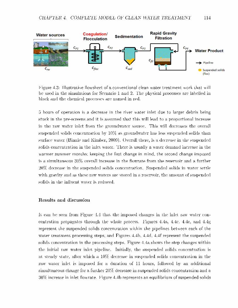
CHAPTER 4. COMPLETE MODEL OF CLEAN WATER TREATMENT 114
Figure 4.3: Illustrative �owsheet of a conventional clean water treatment work that willbe used in the simulations for Scenario 1 and 2. The physical processes are labelled inblack and the chemical processes are named in red.
5 hours of operation is a decrease in the river water inlet due to larger debris being
stuck in the pre-screens and it is assumed that this will lead to a proportional increase
in the raw water inlet from the groundwater source. This will decreases the overall
suspended solids concentration by 10% as groundwater has less suspended solids than
surface water (Binnie and Kimber, 2009). Overall there, is a decrease in the suspended
solids concentration in the inlet water. There is usually a water demand increase in the
warmer summer months; keeping the �rst change in mind, the second change imposed
is a simultaneous 30% overall increase in the �owrate from the reservoir and a further
20% decrease in the suspended solids concentration. Suspended solids in water settle
with gravity and as these raw waters are stored in a reservoir, the amount of suspended
solids in the in�uent water is reduced.
Results and discussion
It can be seen from Figure 4.4 that the imposed changes in the inlet raw water con-
centration propagates through the whole process. Figures 4.4a, 4.4c, 4.4e, and 4.4g
represent the suspended solids concentration within the pipelines between each of the
water treatment processing steps, and Figures 4.4b, 4.4d, 4.4f represent the suspended
solids concentration in the processing steps. Figure 4.4a shows the step changes within
the initial raw water inlet pipeline. Initially, the suspended solids concentration is
at steady state, after which a 10% decrease in suspended solids concentration in the
raw water inlet is imposed for a duration of 11 hours, followed by an additional
simultaneous change for a further 20% decrease in suspended solids concentration and a
30% increase in inlet �owrate. Figure 4.4b represents an equilibrium of suspended solids

CHAPTER 4. COMPLETE MODEL OF CLEAN WATER TREATMENT 115
Table 4.1: Plant data for Scenarios 1 - 3 (initial suspended solids concentration forScenarios 1 and 2 is 6 mg/L and for Scenario 3 the initial suspended solids concentrationis 4500 mg/L).
Pipelines Coagulation/Flocculation (Argaman, 1971)
Cn0 Initial primary particle
concentration (mg/L)
6∗
4500∗∗KA Collision constant (-) 1.8 x 10⁻⁵
Vu Velocity (m/s) 0.003 KB Break-up constant (s) 0.8 x 10⁻⁷
A Area (m2) 20 G Velocity Gradient (s−1) 20
L Length (m) 10∗∗∗ L Length (m) 6
Clari�cation (Burger and Concha, 1998) Filtration (Han et al., 2008)
H Height of clari�cation zone
(m)
-1 L Filter bed depth (m) 0.9
B Depth of thickening zone (m) 3 dc Clean grain diameter (m) 0.8 x 10⁻³
A Area (m2) 400 dp Particle diameter (m) 4 x 10⁻⁶
Cmax Maximum concentration
(mg/L)
7.5 ε0 Porosity (-) 0.4
v0 Settling velocity of a single
particle in unbounded �uid
(m/s)
3.47 α Particle/�lter grain
attachment e�ciency (-)
0.9
r Parameter in equation for
fbk (L/mg)
9.64 x
10−4
αp,
ηp, β
Single parameter (-) 0.9
α1 Parameter in equation for
fbk (m−1)
0.0023 $0 Detachment coe�cient
constant (-)
200
α2 Parameter in dispersion
coe�cient (s/m2)
6.9 x
10−7
σc Critical speci�c deposit
(mg/L)
300
Qu Under�ow volumetric
�owrate (m3/s)
0.4 * Qf ρp Particle density (mg/L) 1350 x 103
γ0 Constant (-) 30
h0 Clean headloss (m) 0.4
*Initial suspended solids concentration for Scenarios 1 and 2
**Initial suspended solids concentration for Scenario 3
***An average of pipeline distance for water treatment works (DEFRA, 2014)

CHAPTER 4. COMPLETE MODEL OF CLEAN WATER TREATMENT 116
Figure 4.4: Scenario 1 - Concentration of suspended solids (mg/L) in each unit of anoverall plant over the course of 24 hours. The simulation begins at steady state, a stepchange of a 10% decrease in suspended solids concentration in the raw water inlet for aduration of 11 hours, then another step change for a further 20% decrease in suspendedsolids concentration and a 30% increase in inlet �owrate imposed.a) Shows the suspended solids concentration (mg/L) in the raw water inlet pipeline.b) Shows the suspended solids concentration (mg/L) in the �occulation unit.c) Shows the suspended solids concentration (mg/L) in the �occulation unit exitpipeline.d) Shows the suspended solids concentration (mg/L) in the clari�cation unit.

CHAPTER 4. COMPLETE MODEL OF CLEAN WATER TREATMENT 117
Figure 4.4 continued: Scenario 1 - Concentration of suspended solids (mg/L) in eachunit of an overall plant over the course of 24 hours. The simulation begins at steadystate, a step change of a 10% decrease in suspended solids concentration in the raw waterinlet for a duration of 11 hours, then another step change for a further 20% decrease insuspended solids concentration and a 30% increase in inlet �owrate imposed.e) Shows the suspended solids concentration (mg/L) in the clari�cation unit exitpipeline.f) Shows the suspended solids concentration (mg/L) in the �ltration unit.g) Shows the suspended solids concentration (mg/L) in the �ltration unit exit pipeline.

CHAPTER 4. COMPLETE MODEL OF CLEAN WATER TREATMENT 118
concentration between the primary and secondary (�ocs) particle phases. There is an
initial decrease in the concentration of �ocs being formed due to the decrease of the
raw water inlet suspended solids concentration, which leads to a second order change in
the clari�cation unit (Figure 4.4d) as can be seen by the collection of suspended solids
concentration in bottom of the tank (axial position 3 m). As there are less �ocs being
formed, there are fewer suspended solids settling in the clari�cation unit, as can also
be seen from the decrease in the concentration of particles settling in the clari�cation
unit, which eventually reaches a new steady state. Within the �ltration unit (Figure
4.4f), there is a steady increase in suspended solids concentration: this is due to the
assumption (Han et al., 2008) that the �ltration unit is used after back-wash, which
enables a greater deposition of particles onto the surface, and with this scenario, the
�ltration unit remains in the ripening stage.
With the second imposed change of 20% decrease in suspended solids concentration and
a 30% increase in inlet �owrate propagating through the system, it is evident that even
with the further decrease in the suspended solids concentration, the increased velocity
a�ects the suspended solids concentration that is carried through the process, as can be
seen in the pipeline exiting the �occulation unit (Figure 4.4c), clari�cation (Figure 4.4e)
and �ltration unit (Figure 4.4g). It is important to note that a decrease in raw water
inlet concentration can have a negative impact on the water purity if the number of
primary particles entering is not su�cient to create �ocs in the coagulation/�occulation
unit, in which case these smaller particles will go through to the clari�cation unit. As
there are more small suspended solids-to-�oc ratio, the small particles will not settle
to sludge and may pass through to the �ltration unit. In theory, this can make the
�ltration unit saturate at a faster rate (Fitzpatrick, 1998), leading to cloudy water
being sent to consumer taps. The impact of the second change particularly a�ected
the clari�cation unit (Figure 4.4d), as the �occulation/coagulation unit relies on the
primary concentration of particles to form �ocs and the clari�cation unit uses the weight
of the �ocs as a form of separation.
4.3.2 Scenario 2
This scenario considers 24 hrs of operation of a water treatment plant that utilises
raw water from a nearby river and groundwater that has been stored in a reservoir
within the winter season. The �rst change imposed (at 5 hours) is an increase in the
raw water suspended solids concentration due to early rainfall. Parsons and Je�erson

CHAPTER 4. COMPLETE MODEL OF CLEAN WATER TREATMENT 119
(2006) state that with continual rainfall, the raw water turbidity and suspended solids
concentration increases signi�cantly by approximately 40%. The second change (at 16
hours) is an increase in water demand so the raw water �owrate from the reservoir is
increased by 20% (to accommodate for the demand) with an accompanying 10% increase
in suspended solids concentration. The increase in the suspended solids concentration
is to account for the additional raw water turbidity and suspended solids concentration
due to the raw water being used in combination with the highly turbid rain water.
Results and discussion
It can be seen from Figure 4.5 that the imposed changes in the inlet raw water con-
centration propagates through the whole process. Figures 4.5a, 4.5c, 4.5e, and 4.5g
represent the suspended solids concentration within the pipelines between each of the
water treatment processing steps and Figures 4.5b, 4.5d, 4.5f represent the suspended
solids concentration in the processing steps. Figure 4.5a shows the step changes within
the initial raw water inlet pipeline; initially, the simulations begin at initial steady state,
after which a 40% increase in suspended solids concentration in the raw water inlet for
a duration of 11 hours is imposed and then another additional change for a further 10%
increase in suspended solids concentration and a 20% increase in inlet �owrate occurs.
The �occulation graph in Figure 4.5b represents an equilibrium of suspended solids
concentration between the primary and secondary (�ocs) particle phases. There is a
substantial increase in the concentration of �ocs being formed due to the decrease of the
raw water inlet suspended solids concentration, which leads to a second order change
in the clari�cation unit (Figure 4.5d) as can be seen by the collection of suspended
solids concentration at the bottom of the tank (axial position 3 m). The impact
of rainfall means the under�ow from the clari�cation unit will have an increase in
suspended solids concentration, and with this increase the sludge height may to increase
with the increasing suspended solids concentration settling, which can contribute to a
higher concentration of suspended solids in the e�uent pipe. Within the �ltration unit
(Figure 4.5f), there is a gradual increase in concentration: this is once again due to the
assumption that the �ltration unit is used after back-wash. The slight suspended solids
concentration increase, indicates the beginning of the breakthrough stage, and as a
result the increased suspended solids concentration and velocity enables the suspensions
to escape with e�uent waters more easily. Moreover, in this scenario (and evident in
Scenario 1) the �ltration unit is not hugely impacted by the imposed changes. This
is due to the majority of the suspended solids concentration being removed in the
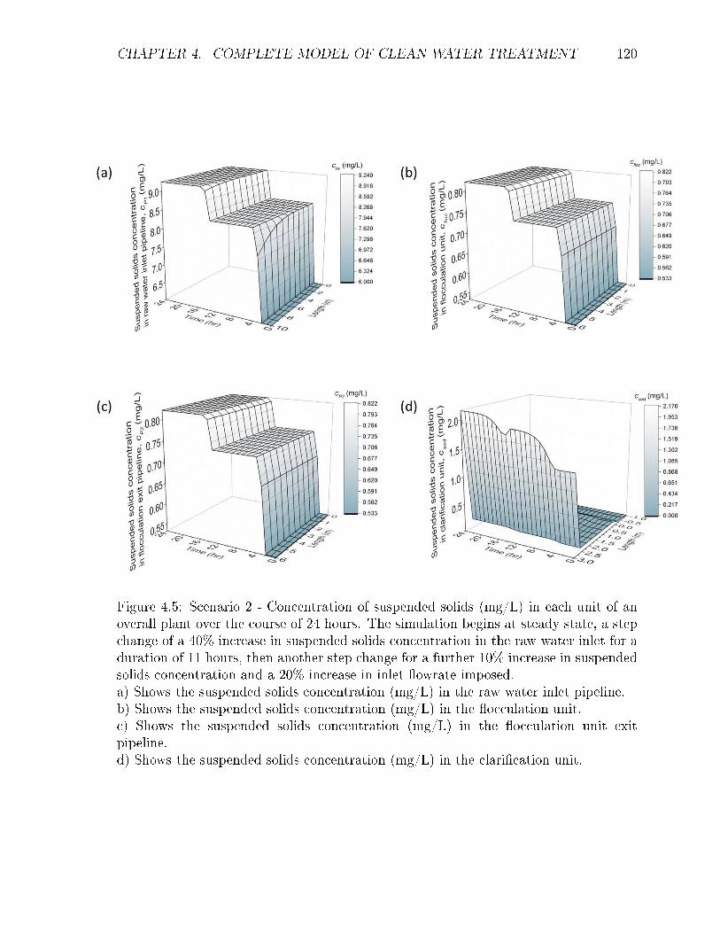
CHAPTER 4. COMPLETE MODEL OF CLEAN WATER TREATMENT 120
Figure 4.5: Scenario 2 - Concentration of suspended solids (mg/L) in each unit of anoverall plant over the course of 24 hours. The simulation begins at steady state, a stepchange of a 40% increase in suspended solids concentration in the raw water inlet for aduration of 11 hours, then another step change for a further 10% increase in suspendedsolids concentration and a 20% increase in inlet �owrate imposed.a) Shows the suspended solids concentration (mg/L) in the raw water inlet pipeline.b) Shows the suspended solids concentration (mg/L) in the �occulation unit.c) Shows the suspended solids concentration (mg/L) in the �occulation unit exitpipeline.d) Shows the suspended solids concentration (mg/L) in the clari�cation unit.

CHAPTER 4. COMPLETE MODEL OF CLEAN WATER TREATMENT 121
Figure 4.5 continued: Scenario 2 - Concentration of suspended solids (mg/L) in eachunit of an overall plant over the course of 24 hours. The simulation begins at steadystate, a step change of a 40% increase in suspended solids concentration in the raw waterinlet for a duration of 11 hours, then another step change for a further 10% increase insuspended solids concentration and a 20% increase in inlet �owrate imposed.e) Shows the suspended solids concentration (mg/L) in the clari�cation unit exitpipeline.f) Shows the suspended solids concentration (mg/L) in the �ltration unit.g) Shows the suspended solids concentration (mg/L) in the �ltration unit exit pipeline.
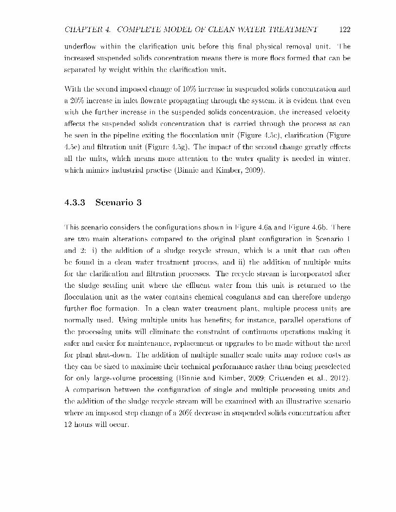
CHAPTER 4. COMPLETE MODEL OF CLEAN WATER TREATMENT 122
under�ow within the clari�cation unit before this �nal physical removal unit. The
increased suspended solids concentration means there is more �ocs formed that can be
separated by weight within the clari�cation unit.
With the second imposed change of 10% increase in suspended solids concentration and
a 20% increase in inlet �owrate propagating through the system, it is evident that even
with the further increase in the suspended solids concentration, the increased velocity
a�ects the suspended solids concentration that is carried through the process as can
be seen in the pipeline exiting the �occulation unit (Figure 4.5c), clari�cation (Figure
4.5e) and �ltration unit (Figure 4.5g). The impact of the second change greatly e�ects
all the units, which means more attention to the water quality is needed in winter,
which mimics industrial practise (Binnie and Kimber, 2009).
4.3.3 Scenario 3
This scenario considers the con�gurations shown in Figure 4.6a and Figure 4.6b. There
are two main alterations compared to the original plant con�guration in Scenario 1
and 2: i) the addition of a sludge recycle stream, which is a unit that can often
be found in a clean water treatment process, and ii) the addition of multiple units
for the clari�cation and �ltration processes. The recycle stream is incorporated after
the sludge settling unit where the e�uent water from this unit is returned to the
�occulation unit as the water contains chemical coagulants and can therefore undergo
further �oc formation. In a clean water treatment plant, multiple process units are
normally used. Using multiple units has bene�ts; for instance, parallel operations of
the processing units will eliminate the constraint of continuous operations making it
safer and easier for maintenance, replacement or upgrades to be made without the need
for plant shut-down. The addition of multiple smaller scale units may reduce costs as
they can be sized to maximise their technical performance rather than being preselected
for only large-volume processing (Binnie and Kimber, 2009; Crittenden et al., 2012).
A comparison between the con�guration of single and multiple processing units and
the addition of the sludge recycle stream will be examined with an illustrative scenario
where an imposed step change of a 20% decrease in suspended solids concentration after
12 hours will occur.

CHAPTER 4. COMPLETE MODEL OF CLEAN WATER TREATMENT 123
Figure 4.6: Illustrative �owsheet of a conventional clean water treatment work thatwill be used in the simulations for scenario 3 incorporating a sludge recycle unit. Thephysical processes are labelled in black and the chemical processes are named in red.a) Single processing units.b) Expansion of Figure 4.6a incorporating multiple processing units in parallel forclari�cation and �ltration.
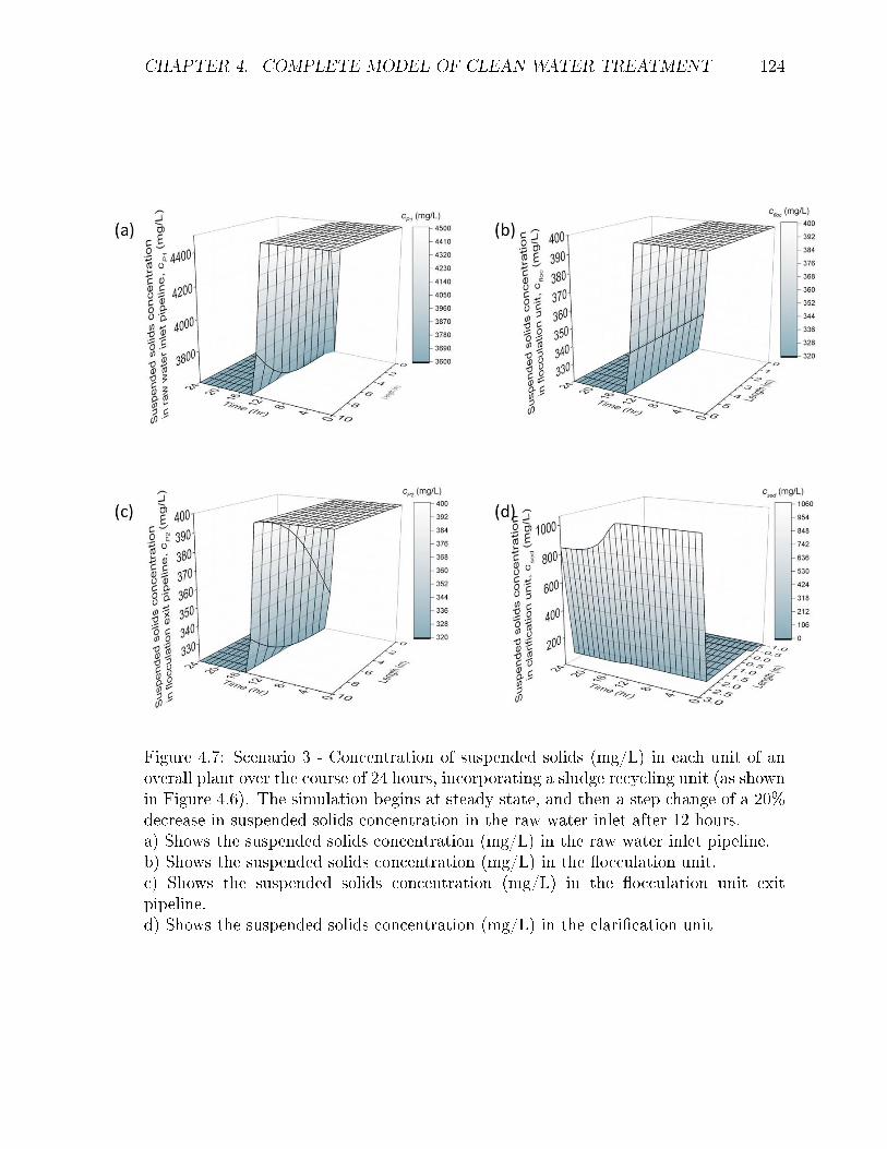
CHAPTER 4. COMPLETE MODEL OF CLEAN WATER TREATMENT 124
Figure 4.7: Scenario 3 - Concentration of suspended solids (mg/L) in each unit of anoverall plant over the course of 24 hours, incorporating a sludge recycling unit (as shownin Figure 4.6). The simulation begins at steady state, and then a step change of a 20%decrease in suspended solids concentration in the raw water inlet after 12 hours.a) Shows the suspended solids concentration (mg/L) in the raw water inlet pipeline.b) Shows the suspended solids concentration (mg/L) in the �occulation unit.c) Shows the suspended solids concentration (mg/L) in the �occulation unit exitpipeline.d) Shows the suspended solids concentration (mg/L) in the clari�cation unit

CHAPTER 4. COMPLETE MODEL OF CLEAN WATER TREATMENT 125
Figure 4.7 continued: Scenario 3 - Concentration of suspended solids (mg/L) in eachunit of an overall plant over the course of 24 hours, incorporating a sludge recyclingunit (as shown in Figure 4.6). The simulation begins at steady state, and then a stepchange of a 20% decrease in suspended solids concentration in the raw water inlet after12 hours.e) Shows the suspended solids concentration (mg/L) in the clari�cation unit exitpipeline.f) Shows the suspended solids concentration (mg/L) in the �ltration unit.g) Shows the suspended solids concentration (mg/L) in the �ltration unit exit pipeline.

CHAPTER 4. COMPLETE MODEL OF CLEAN WATER TREATMENT 126
Figure 4.8: Scenario 3 - Concentration of suspended solids (mg/L) in each unit of anoverall plant over the course of 24 hours, incorporating multiple processing units forclari�cation and �ltration incorporating a sludge recycle unit (as shown in Figure 4.6b).The simulation begins at steady state, and then a step change of a 20% decrease insuspended solids concentration in the raw water inlet after 12 hours.a) Shows the suspended solids concentration (mg/L) in the raw water inlet pipeline.b) Shows the suspended solids concentration (mg/L) in the �occulation unit.c) Shows the suspended solids concentration (mg/L) in the �occulation unit exitpipeline.d) Shows the suspended solids concentration (mg/L) in the clari�cation unit.

CHAPTER 4. COMPLETE MODEL OF CLEAN WATER TREATMENT 127
Figure 4.8 continued: Scenario 3 - Concentration of suspended solids (mg/L) in eachunit of an overall plant over the course of 24 hours, incorporating multiple processingunits for clari�cation and �ltration incorporating a sludge recycle unit (as shown inFigure 4.6b). The simulation begins at steady state, and then a step change of a 20%decrease in suspended solids concentration in the raw water inlet after 12 hours.e) Shows the suspended solids concentration (mg/L) in the clari�cation unit exitpipeline.f) Shows the suspended solids concentration (mg/L) in the �ltration unit.g) Shows the suspended solids concentration (mg/L) in the �ltration unit exit pipeline.

CHAPTER 4. COMPLETE MODEL OF CLEAN WATER TREATMENT 128
Results and discussion
Figure 4.7 shows the propagation of an imposed step change of a 20% decrease in
suspended solids concentration through a clean water treatment plant with a single unit
con�guration (as shown in Figure 4.6a) whilst Figure 4.8 shows the propagation through
a multiple unit con�guration (as show in Figure 4.6b). The coagulation/�occulation
unit is singular in both scenarios and the resulting concentration and propagation
through this unit is the same however the units following show some interesting results.
Figure 4.6b assumes that the �ow is split equally by the number of units, in this case
3 units; however this might not necessarily be the case in real life as the pipelines
connecting units are not in ideal conditions. The �rst observation to note is that with
the use of multiple units, the concentration exiting each unit (Figure 4.8c, 4.8e, 4.8g) is
substantially decreased; this implies that the area for these units can be made smaller,
which in reality would make the units easier to manage. The addition of multiple units
also indicates there is a decrease in suspended solids concentration in the under�ow
leaving from a single clari�cation unit to the sludge stream, which may aid in the
prevention of pipe blockage due to an over�ow of suspended solids being concentrated
in one unit.
Focusing on the concentration of suspended solids particles exiting the clari�cation unit
(Figure 4.8e), the amount of suspended solids that leaves each of the clari�cation units
is shown to be signi�cantly smaller than the amount that leaves in Figure 4.7e. This has
an e�ect on the behaviour of the �ltration unit, in the sense that when there is a single
�ltration unit, there is an indication that the unit is beginning to enter the �working�
stage as there is a returning curve around t = 4 hrs. However, this phenomenon is
not present in Figure 4.8f, meaning that the �ltration system would be able to last
for a longer time period without the need for a back-wash to clean the �lters. The
�nal exit suspended solids concentration (Figure 4.8g) is also lower in the multiple
con�guration system by a magnitude of 10 and this suggests the reduced concentration
and �ow demands when using multiple units the areas can be increased which may lead
to signi�cant saving in the overall capital costs of a new infrastructure.
4.4 Computational statistics
All three scenarios were simulated using gPROMS 4.2 (Process Systems Enterprise,
2014) on a Dell OptiPlex 990MT workstation with 3.1 GHz processor, 4GB RAM and

CHAPTER 4. COMPLETE MODEL OF CLEAN WATER TREATMENT 129
Table 4.2: Computational statistics of clean water treatment Scenarios 1 - 3.
Without sludge recycle
Scenario 1 Scenario 2
Variables 926 926Equations 1200 1200
CPU Time (s) 0.87 (14% system time) 0.58 (11% system time)
With sludge recycle (Scenario 3)
Single unit �owsheet Multiple unit �owsheet
Variables 1010 2665Equations 1286 3371
CPU Time (s) 1.48 (13% system time) 13.84 (87% system time)
Windows 7 64-bit operating system. The computational statistics of all three scenarios
are shown in Table 4.2. Scenarios 1 and 2 have the same number of variables and
equations as the only change are the numerical values of the proposed step changes.
Scenario 1 has a larger CPU time (0.87 s) than Scenario 2 (0.58 s) and this di�erence
can be attributed to the simulation accounting for the second step change in Scenario 1
which incorporates both a decrease in suspended solids concentration with an increase
in the �owrate. Many large scale water treatment plants include at least one recycle
stream for water recovery. When a recycle is included in the single unit model the time
to �nd an optimal solution is 1.48 seconds. The increased CPU when a recycle stream
is added is expected additional equations and variables have been added. The addition
of a recycle stream is not the only increase in CPU, additional units in parallel also
increase the computational time needed.
4.5 Conclusion
This chapter has presented an overall mathematical model of a clean water treatment
plant by combining together models of individual processing units which have been
previously studied in isolation. The detailed models developed in Chapter 3 have been
combined in order to simulate an overall conventional clean water treatment model.
The overall model can be used at an early stage of process development for design
purposes as a training tool for plant operators, or to investigate the consequences of
changes in the plant.
It has been demonstrated that the developed model is able to predict the behaviours of

CHAPTER 4. COMPLETE MODEL OF CLEAN WATER TREATMENT 130
the plant following an imposed changes in the raw water suspended solids concentration.
Three di�erent scenarios were presented with three alternative clean water treatment
con�gurations; namely, single processing units, multiple processing units and the ad-
dition of a sludge recycle stream. The scenarios presented considered a blend of raw
water sources from surface water and groundwater that have been stored in a reservoir
during both the summer and winter months, each with varying step changes imposed.
The changes, when imposed, were successfully propagated through the clean water
treatment process simulation. For a model like this to be fully utilised, it needs to be
operator friendly, and the detailed mathematical models shown so far are complex and
the simulations require specialist software and computational capabilities. With this
in mind, the next chapter addresses the development of simpler, or �surrogate� models,
which are easier to use and require less sophisticated solution methods.

Chapter 5
Surrogate models for process
integration
In this chapter, the development of novel surrogate models from detailed
mathematical models will be discussed for the process units considered in
previous chapters. A major bene�t of surrogate modelling is simplistic mod-
els that can be implemented in the water treatment process. Detailed models
are complex and require specialist knowledge in computational tools that
surrogate models will overcome. After the development of the surrogate
models, their ability to predict mechanistic trends will be veri�ed against
the detailed models developed in chapter 3.
5.1 Introduction
Chapter 3 presented detailed dynamic mathematical models for a number of individual
water treatment processes. These are complex models based fundamental knowledge
and are only concerned with the phenomena occurring within the individual process
units. Linking these dynamic models together into an overall plant model increased the
complexity. This resulted in a challenging equation system which could prove di�cult
for operators to use on a water treatment plant. This can be resolved through the use
of simpli�ed surrogate models that are generated by the detailed models but with less
complexity which will therefore reduce the computational expertises and time needed.
131

CHAPTER 5. SURROGATE MODELS FOR PROCESS INTEGRATION 132
5.2 Surrogate modelling
Surrogate models, developed through regression analysis, are black box models which
are generated from data either sourced experimentally or obtained from a highly-accurate
and computationally expensive models. Regression analysis predicts continuous output
or response variables from various independent input variables by approximating their
functional relationship (Yang et al., 2016). Surrogate models built with a large number
of data points are generally more accurate than models with a reduced number of data
points, due to limited information. The surrogate models built with less data points are
able to predict output variables from relevant input variables without providing details
of the complex mechanisms (Box and Draper, 1987; Davis and Ierapetritou, 2008; Bai
et al., 2014); however, bias results may be produced with a surrogate model built
from approximate information. It is more bene�cial to have an understanding of the
true underlying functional relationship with variables that is o�ered by detailed mod-
els. If detailed computationally expensive simulations are replaced with approximate
mathematical models, then much more data points can be generated through repeated
simulations. With simpler functions, regression analysis is able to approximate the
overall system behaviour whilst preserving the desired level of accuracy (Caballero and
Grossmann, 2008; Henao and Maravelias, 2010, 2011; Beck et al., 2012).
In literature, several regression analysis methodologies exist, including: Kriging (Kleijnen
and Beers, 2004; Kleijnen, 2009), Radial Basis Functions (RBF) (Sarimveis et al., 2004),
Multivariate Adaptive Regression Splines (MARS) (Friedman, 1991), and Support
Vector Regression (SVR) (Smola, 2004; Levis and Papageorgiou, 2005; Forrester and
Keane, 2009).
The two most common methods utilised in water quality modelling are arti�cial neutral
networks (ANN) (Zhang and Stanley, 1999; Raman and Sunilkumar, 1995; Hamed et al.,
2004; Cordoba et al., 2014) and polynomial response surface (linear and multi-variable
linear regression) (Sadiq and Rodriguez, 2004; Chenini and Khemiri, 2009). The main
di�erence between these two methods is that ANN creates mapping sequences between
input and output datasets obtained from the process. The mapping between the input
and outputs is achieved using historical data to train the network, which is utilised to
create the architecture required to predict process outputs for any data that is not used
as the training set. ANNs require a larger dataset to bene�t from its optimisation,
if enough data is not provided then irrespective of the existing non-linearities, linear
regression model may be better adjusted. These two methodologies will summarised
brie�y before the selected method is discussed in detail.

CHAPTER 5. SURROGATE MODELS FOR PROCESS INTEGRATION 133
Figure 5.1: Typical structure of a feedforward arti�cial neural network (ANN).
5.2.1 Arti�cial neural network
An arti�cial neutral network (ANN) is a developed mathematical model or algorithm
that is inspired by the operations of the biological nervous system (biological neural
networks) (Hill et al., 1994). In other words, patterns are found in data utilising the
functioning of neutral networks as non-linear statistical data modelling tools used to
model complex relationships between inputs and outputs. Generally, in the learning
phase, an ANN is adaptive and can change its structure based on external or internal
information that �ows through the network. Ultimately, knowledge is gained by the
network through a learning process and the interconnections between the elements of
the network store the knowledge (Gernaey et al., 2004). When there is a lot of training
data available, ANN are especially useful for function-approximating problems (Gevrey
et al., 2003). Trained with su�cient data, ANN can su�ciently describe multivariate
systems with non-linear dynamics (Dua, 2010).
The general format for an ANN structure is presented in Figure 5.1, which shows a
typical feedforward ANN. The relationships between the input layer, the hidden layer
and the output layer are connected with weighted links and the nodes have biases, both
of these aspects represent the system parameters (Prasad and Bequette, 2003). The
ANN receives information through the input layer; this information is processed and
sent to the hidden layer. Computationally, the hidden layer processes the information
further and this data is sent to the output layer which provides the information of the
process system. Generally, the nodes in the input layer receive information from the
training/validation datasets, whilst the nodes in the hidden and output layers receive

CHAPTER 5. SURROGATE MODELS FOR PROCESS INTEGRATION 134
information directly from the nodes in the preceding layer of the network. Within the
wastewater sector, ANN has been used to describe the biochemical processes in the
biological wastewater treatment (Hamoda et al., 1999; Gontarski et al., 2000; Mjalli
et al., 2007).
5.2.2 Polynomial response surface methodology
Response surface methodology (RSM) is a series of mathematical and statistical tech-
niques that are useful for developing, improving and optimising di�erent processes
(Gunst, 1996). It identi�es polynomial equations that can describe the relationship
between input (independent variables) and output (response) data. RSM was initially
developed to model responses of experiments (Box and Draper, 1987), it was then
further developed to numerical experiment modelling (Toropov and Markine, 1996).
The application of RSM to design optimisation is aimed at reducing computational
costings of expensive analysis methods (e.g. �nite element method or CFD analysis)
in addition to their associated numerical noise (Khayet et al., 2008). In general, the
structure of the relationship between the independent variables and the response is
unknown.
The end goal of RSM is to �nd a suitable approximation to the true functional rela-
tionship between dependent and independent variables. The most common forms are
low-order polynomials (�rst or second-order), where second-order models are usually
su�cient to re�ect the data and trends of more complex models as they are very �exible
and can easily estimate the parameters using the least-square method. The general
governing equation for a second-order multiple polynomial regression model is:
Z = β0 + βixi + βjxj + βiix2i + βjjx
2j + βijxixj (5.2.1)
Where:
Z predicted response
β0 constant coe�cient
βi linear interaction coe�cient
βii , βij quadratic interaction coe�cients
xi, xj input variables in�uencing predicted response Z
The main purposes of these types of models are (Draper, 1997):

CHAPTER 5. SURROGATE MODELS FOR PROCESS INTEGRATION 135
1. To establish an approximate relationship between Y and x1,x2,...,xk that can be
used to predict response values for given settings of input variables, Yi.
2. To determine the level of signi�cance of the factors with levels represented by
x1,x2,...,xk.
3. To determine the optimum settings of x1,x2,...,xk that result in the maximum or
minimum response over a certain region of interest.
The method of least squares is typically used to estimate the regression coe�cients,
β, in a multi-linear regression model. It is simpler to solve Equation 5.2.1 in matrix
notation which is given by (Draper, 1997):
β =
β0
...
βk
Z =
Z1
...
Zn
X =
1 x11 x12 · · · x1k
1 x21 x22 · · · x2k
......
... · · · ......
...... · · · ...
......
... · · · ...
1 xn1 xn2 · · · xnk
∀i = 1...k
∀j = 1...n(5.2.2)
In general, β is a k×1 vector of the regression coe�cients, Z is an n×1 vector of the
observations and X is an n×k model matrix consisting of the expanded independent
variables. Thus, Equation 5.2.1 may be expressed as (Edgar et al., 1989):
XTXβ = XTZ
when re-arranged the least-squares estimator of β can be written as (Edgar et al., 1989):
β =(XTX
)−1XTZ
In scalar notation, the �tted model is:
Z = β0 +K∑i=1
βixi +∑i<j
βijxixj +K∑i=1
βiix2i (5.2.3)
5.2.3 Full factorial design
Factorial designs can be used for �tting �rst- and second-order models. The accuracy
of the approximation and the time taken to construct the response surface is largely

CHAPTER 5. SURROGATE MODELS FOR PROCESS INTEGRATION 136
in�uenced by the choice of the design of experiments (Montgomery, 1997). In this work,
the factorial design strategy will be used to transform the detailed mathematical models
into quadratic surrogate models. From previous chapters, in�uential variables are
identi�ed for the various detailed process models. Within the factorial design strategy,
the design variables are varied together instead of focusing on each one individually.
To build an approximation model to capture k design variables, the upper and lower
bounds of each design variables need to be de�ned to create the desired range. This is
followed by discretisation of the desired range, two and three levels are more commonly
used. Two levels (called 2k full factorial) require the ranges to be de�ned by only the
lower and upper bounds whilst three levels (also known as 3k full factorial) include
mid-points. The development of a quadratic response surface model in k variables
requires three levels so that the interaction coe�cients can be estimated and the model
will be able to �t curved response functions (Montgomery, 1997), as will be considered
in this work.
For simultaneous optimisation using response surface modelling, each input variable,
Y i, and normalised variable, xi, must have a low, centre and high value assigned to
each goal. For a goal of maximum, the desirability curve is given by:
xi =[
Yi−YLowiYHighi−YLowi
], YLowi ≤ Yi ≤ YHighi ∀i = 1...k (5.2.4)
For a goal of centre, the desirability curve is given by:
xi =[
Yi−YCentreiYCentrei−YLowi
], YLowi ≤ Yi ≤ YCentrei
YCentrei ≤ Yi ≤ YHighi∀i = 1...k (5.2.5)
orxi =
[Yi−YCentrei
YHighi−YCentrei
], YLowi ≤ Yi ≤ YCentrei
YCentrei ≤ Y i ≤ YHighi∀i = 1...k (5.2.6)
For a goal of minimum, the desirability curve is given by:
xi =[
YHighi−Y iYHighi−YLowi
], YLowi ≤ Yi ≤ YHighi ∀i = 1...k (5.2.7)
Draper (1997) and Montgomery (1997) presented a methodology to develop surrogate
models from data provided.
1. The number of runs required to ensure all the combination of variables, k, and

CHAPTER 5. SURROGATE MODELS FOR PROCESS INTEGRATION 137
levels, n, are considered can be calculated by:
No. runs = nk (5.2.8)
2. Develop a coded matrix X, where all the levels (low, centre and high) are repres-
ented by -1, 0 and 1, respectively.
3. Use the detailed mathematical models to determine a value for Z, for a given set
of independent variables, k.
4. Determine the transpose matrix, XT , and calculate (XTX)−1.
5. Calculate the transpose matrix, XT multiplied by Z, (XTZ).
6. Solve for the least squares estimator of β.
In the next section, the methodology detailed above is used to develop the surrogate
models for calculating the e�uent suspended solids concentration in each of the pro-
cessing units considered in Chapter 3. The polynomial response surface methodology
will be used as the limitation with the using ANN in this work is the lack of su�cient
plant data to create an adequate system. The developed surrogate models will be tested
against the detailed models within the desired range, between the low and high goals,
to validate their use by checking the accuracy of the �t utilising parity plots, and values
outside of the desired range to explore how these models will react.
5.3 Coagulation-�occulation surrogate model
In Chapter 3, two detailed mathematical models were developed in sub-section 3.2.2 to
represent the unit processes of rapid mixing and �occulation in chambers/compartments
for the coagulation/�occulation process.
Rapid Mixing
In this section, a surrogate model will be developed which links two key variables
to the e�uent suspended solids concentration. The sensitivity analysis conducted in
sub-section 3.2.2 showed that the suspended solids concentration in the rapid mixing

CHAPTER 5. SURROGATE MODELS FOR PROCESS INTEGRATION 138
unit was a�ected by the inlet (primary) suspended solids concentration and the speed
at which suspended solids were mixed. Using Equation 5.2.1, the polynomial equation
will take on the form:
cfloc,RM = β0 + β1x1 + β2x2 + β11x21 + β22x
22 + β12x1x2 (5.3.1)
where
cFloc,RM output e�uent suspended solids concentration, (mg/L)
x1 normalised initial suspended solids, (mg/L)
x2 normalised velocity gradient, (s−1)
As explained in sub-section 5.2.2, the two factors, x1 and x2, will be explored at three
di�erent levels (low, centre and high) with the goal of �nding an average desirability
range. By using Equation 5.2.5, the following expressions will be used to determine the
factors for each variable, e.g.:
x1 =
[c0 − c0centre
c0centre − c0low
](5.3.2)
x2 =
[G−Gcentre
Gcentre −Glow
](5.3.3)
where
c0 initial suspended solids values used in detailed model, (mg/L)
G velocity gradient values used in detailed model, (s−1)
Utilising the methodology detailed in Section 5.2.2, Equation 5.2.8 shows there are 9
simulations needed in order to have all combinations. Table 5.1 presents the typical
ranges of operation that were considered to ensure the level of accuracy, and the
justi�cations for the choices.
Once these variables were speci�ed, the detailed models were simulated with the di�er-
ent combinations of variable values to obtain an e�uent suspended solids concentration.
Formulas programmed into Microsoft Excel are then utilised to develop the surrogate
models using steps 2 to 7. Table 5.2 presents the numerical values for the least squares
estimator, β, for coagulation/�occulation via rapid mixing. The values are provided
as both "unlogged" and "logged"1 due to a log scale making it easy to compare values
that cover a large range.
1For ease of interpretation, the logarithmic transformation of models in the text are referred to as�logged � and the regular model notation is referred to as �unlogged�.
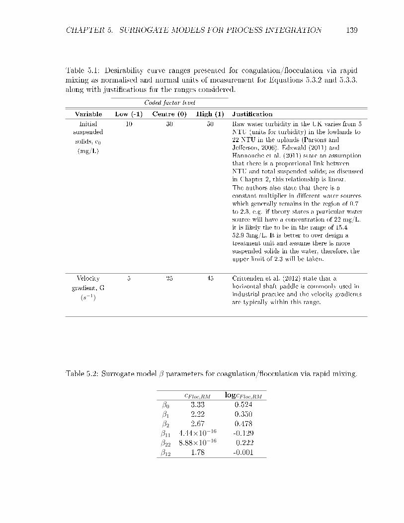
CHAPTER 5. SURROGATE MODELS FOR PROCESS INTEGRATION 139
Table 5.1: Desirability curve ranges presented for coagulation/�occulation via rapidmixing as normalised and normal units of measurement for Equations 5.3.2 and 5.3.3,along with justi�cations for the ranges considered.
Coded factor level
Variable Low (-1) Centre (0) High (1) Justi�cation
Initialsuspended
solids, c0
(mg/L)
10 30 50 Raw water turbidity in the UK varies from 5NTU (units for turbidity) in the lowlands to22 NTU in the uplands (Parsons andJe�erson, 2006). Edzwald (2011) andHannouche et al. (2011) state an assumptionthat there is a proportional link betweenNTU and total suspended solids; as discussedin Chapter 2, this relationship is linear.
The authors also state that there is aconstant multiplier in di�erent water sourceswhich generally remains in the region of 0.7to 2.3, e.g. if theory states a particular watersource will have a concentration of 22 mg/L,it is likely the to be in the range of 15.4 -52.9 3mg/L. It is better to over design atreatment unit and assume there is moresuspended solids in the water, therefore, theupper limit of 2.3 will be taken.
Velocity
gradient, G
(s−1)
5 25 45 Crittenden et al. (2012) state that ahorizontal shaft paddle is commonly used inindustrial practice and the velocity gradientsare typically within this range.
Table 5.2: Surrogate model β parameters for coagulation/�occulation via rapid mixing.
cFloc,RM logcFloc,RMβ0 3.33 0.524β1 2.22 0.350β2 2.67 0.478β11 4.44×10⁻¹⁶ -0.129β22 8.88×10⁻¹⁶ -0.222β12 1.78 -0.001

CHAPTER 5. SURROGATE MODELS FOR PROCESS INTEGRATION 140
The regression equation developed for coagulation/�occulation via rapid mixing, ex-
pressed as the "unlogged" and "logged" values of cFloc,RM are:
cFloc,RM = 3.33 + 2.22x1 + 2.67x2 + 4.44× 10−16x21 + 8.88× 10−16x2
2 + 1.78x1x2 (5.3.4)
logcFloc,RM = 0.524 + 0.35x1 + 0.478x2 − 0.129x21 − 0.222x2
2 − 0.001x1x2 (5.3.5)
The validation and sensitivity analysis of the equations above to predict the e�uent
concentration, cFloc,RM , will be presented in Section 5.3.1.
Flocculation in chambers/compartments
For the coagulation/�occulation unit, an alternative unit operation has been developed
for performance comparison. The rapid mixing unit occurs in a reactor whilst this
�occulation unit takes place in compartments in series. In this section, a surrogate
model will be developed which links four key variables to the e�uent suspended solids
concentration. The sensitivity analysis conducted in sub-section 3.2.2 showed that the
suspended solids concentration in the �occulation unit was a�ected not only by the
inlet (primary) suspended solids concentration and the speed at which these suspended
solids were mixed but also the number of compartments and the time spent in the
compartments (residence time). Using Equation 5.2.1, the polynomial equation will
take on the form:
cfloc,COM = β0 + β1x1 + β2x2 + β3x3 + β4x4 + β11x21 + β22x
22 + β33x
23 + β44x
24
+β12x1x2 + β13x1x3 + β14x1x4 + β23x2x3 + β24x2x4 + β34x3x4
(5.3.6)
where
cFloc,COM e�uent suspended solids concentration, (mg/L)
x1 normalised initial suspended solids concentration values used
in detailed model, (mg/L)
x2 normalised velocity gradient values used in detailed model,
(s−1)
x3 normalised number of compartments values used in detailed
model, (-)
x4 normalised residence time values used in detailed model, (s)
The four factors, x1, x2, x3 and x4 will be explored at three di�erent levels (low, centre
and high) with the goal of �nding an average desirability range. By using Equation

CHAPTER 5. SURROGATE MODELS FOR PROCESS INTEGRATION 141
5.2.5, the following equations will be used to determine the factors for each variable,
i.e.:
x1 =
[c0 − c0centre
c0centre − c0low
](5.3.7)
x2 =
[G−Gcentre
Gcentre −Glow
](5.3.8)
x3 =
[m−mcentre
mcentre −mlow
](5.3.9)
x4 =
[τ − τcentreτcentre − τlow
](5.3.10)
where
c0 initial suspended solids concentration, (mg/L)
G velocity gradient, (s−1)
m number of compartments, (-)
τ residence time, (s)
Utilising the methodology detailed in Section 5.2.2, Equation 5.2.8 shows there are 81
simulations needed in order to have all combinations. Table 5.3 presents the typical
ranges of operation that were considered to ensure the level of accuracy, and the
justi�cations for the choices.
Once these variables are speci�ed, the detailed models are simulated with the di�erent
combinations of variable values to obtain an e�uent suspended solids concentration.
As with rapid mixing, the formulae was programmed in Microsoft Excel then utilised
to develop the surrogate models from steps 2 to 7. Table 5.4 presents the numerical
values for the least squares estimator, β, for coagulation/�occulation via �occulation
in chambers/compartments.
The regression equation developed for �occulation via �occulation chambers/compartments,

CHAPTER 5. SURROGATE MODELS FOR PROCESS INTEGRATION 142
Table 5.3: Desirability curve ranges for coagulation/�occulation via �occulationchambers/compartments presented as input units of measurement for Equations 5.3.7to 5.3.10, along with justi�cations for the ranges considered.
Coded factor level
Variable Low (-1) Centre (0) High (1) Justi�cation
Initialsuspendedsolids, c0
(mg/L)
10 30 50 Same justi�cation as in Table 5.1
Velocity
gradient, G
(s−1)
5 25 45 Same justi�cation as in Table 5.1
Number ofcompart-ment
s, m (-)
3 5 7 In industry, typically �occulation of thisnature typically has multiple compartments,and ba�es are often used to separate thesecompartments, It is assumed that the rangeof compartments in series typically between 3and 7 (Hendricks, 2006).
Residence
time, τ (s)
1200 2100 3000 Crittenden et al. (2012) state that ahorizontal shaft paddle is commonly used inindustrial practice and the residence time istypically within this range.
Table 5.4: Surrogate model β parameters for coagulation/�occulation via �occulationchambers/compartments.
cFloc,COM logcFloc,COMβ0 68.8 1.85β1 51.9 0.349β2 45.4 0.254β3 7.05 0.0238β4 29.01 0.131β11 -0.167 -0.128β22 10.7 -0.0246β33 -2.12 -0.009β44 5.24 0.0053β12 30.2 -4E-05β13 4.59 -0.0007β14 19.3 3.3E-05β23 8.91 0.0259β24 29.4 0.0927β34 6.49 0.0146

CHAPTER 5. SURROGATE MODELS FOR PROCESS INTEGRATION 143
expressed as the "unlogged" and "logged" values of cFloc,COM are:
cFloc,COM = = 68.8 + 59.9x1 + 45.4x2 + 7.05x3 + 29.01x4 − 0.167x21 + 10.7x2
2
−2.12x23 + 5.24x2
4 + 30.2x1x2 + 4.59x1x3 + 19.3x1x4 + 8.91x2x3
+29.4x2x4 + 6.49x3x4
(5.3.11)
logcFloc,COM = 1.85 + 0.349x1 + 0.254x2 + 0.0238x3 + 0.131x4 − 0.128x21
−0.0246x22 − 0.009x2
3 − 0.005x24 + 3.5× 10−5x1x2 − 0.00072x1x3
+3.32E − 05x1x4 + 0.0259x2x3 + 0.0927x2x4 + 0.0146x3x4
(5.3.12)
The validation and sensitivity analysis of the equations above to predict the e�uent
concentration, CFloc,COM , will be presented in Section 5.3.1.
5.3.1 Results and validation
In this section, the surrogate model developed for the coagulation/�occulation unit via
rapid mixing and in chambers/compartments is veri�ed and the response values are
analysed.
Rapid mixing
The regression coe�cient, R2, is the statistical measure of how well the regression
line approximates the data points and here the R2 value compares the detailed model
response with the surrogate model response. By plotting this data, the order of the
relationship between the computational requirement and the number of equations can
be obtained. With both the "logged", logcFloc,RM , and the "unlogged", cFloc,RM , data,
the model �t is very good with a R2 value of 99.9% meaning that either surrogate
model (in the "logged" or "unlogged" form) can describe the process behaviour within
the variable bounds almost as well as the detailed model for the same data set.
Figure 5.2 presents the predicted response for the e�uent suspended solids concen-
tration using the surrogate model against the e�uent suspended solids concentration
determined by the detailed model. In agreement with the R2 coe�cient, for both the
"logged" and "unlogged" model, the surrogate model's predictive capacity seem to be
a very good �t as shown by the almost linear plot and the data points laying close the
x=y line.

CHAPTER 5. SURROGATE MODELS FOR PROCESS INTEGRATION 144
Figure 5.2: Rapid mixing: surrogate versus detailed modelling responses for e�uentconcentration for a) normal model responses and b)"logged" model responses. Thedashed line represent the x=y line on a parity plot.

CHAPTER 5. SURROGATE MODELS FOR PROCESS INTEGRATION 145
Figure 5.3: Coagulation/�occulation via rapid mixing: 2D graphical domainrepresentation of the ranges for the variables and the data used for veri�cation inTable 5.5.
Although, the surrogate models are able to accurately �t data from the detailed model
this, however, does not necessarily mean that the models are able to predict other mech-
anistic trends as the surrogate models were �tted within a speci�c range of variables
(Caballero and Grossmann, 2008; Henao and Maravelias, 2011). The surrogate models
were veri�ed against the detailed rapid mixing model, with variable values inside and
outside of the ranges considered in Table 5.1.
Eight di�erent runs (four inside the range and four outside the range) are simulated
by both the detailed and surrogate models in order to compare the e�uent suspended
solids concentration predicted. Figure 5.3 represents graphically the range in which the
surrogate model is �tted and Table 5.5 provides the data used for the veri�cation of
the surrogate model. Inside of the prediction range, the four runs (1-4) show that the
"unlogged" surrogate model produces a small error when compared with the detailed
model; however, when the "logged" detailed model is compared with the "logged"
surrogate model there is a bigger error. This shows that the "logged" surrogate model
is not as reliable within the prediction range even though the R2 value is the same.
From Table 5.5, it can be seen that the "logged" model does not predict as accurately
as the "unlogged" response values, instead it under/over predicts the e�uent suspended
solids concentration.

CHAPTER 5. SURROGATE MODELS FOR PROCESS INTEGRATION 146
Table 5.5: Veri�cation of e�uent suspended solids concentration derived from "logged"and "unlogged" surrogate model for coagulation/�occulation via rapid mixing againstthe detailed model.
Normal LOGRun c0
(mg/L)
G
(s−1)
DetailedcFloc,RM
(mg/L)
SurrogatecFloc,RM
(mg/L)
Error
%
DetailedcFloc,RM
(mg/L)
SurrogatecFloc,RM
(mg/L)
Error
%
Inside prediction range (10 ≤ c0 ≤ 50 and 5 ≤ G ≤ 45)
1 15 10 0.67 0.665 0.65 -0.17 -0.29 70
2 40 30 5.33 5.338 0.07 0.73 0.77 6.21
3 25 40 4.44 4.44 0.09 0.65 0.66 2.16
4 35 10 1.56 1.555 0.38 0.19 0.12 36
Outside prediction range (c0 < 10, c0 > 50 and G < 5, G > 45)
5 60 25 6.67 6.668 0.03 0.82 0.76 7.94
6 30 100 13.3 13.33 0.25 1.12 -0.81 28
7 5 5 0.11 0.109 0.57 -0.96 -0.82 14.8
8 10 50 2.22 2.224 0.07 0.35 0.29 14.7
This is further shown when observing the response values produced outside of the
prediction range where each run represents one variable being out of the range. Four
runs simulated outside of the prediction range to observe how the models will react
when faced with a variety of variables both inside and outside of the desired ranges:
� Run 5: the initial suspended solids concentration, c0, is higher than the range.
� Run 6: the velocity gradient, G, is more than 200% bigger than the top of the
range.
� Run 7: the initial suspended solids concentration, c0, is lower then the desired
range
� Run 8: the velocity gradient, G, is lower then the desired range.
The largest error (70%) is predicted with the "logged" models especially during Run
1; however, the "unlogged" model is still able to predict to a good extent the response
outside of the prediction range. For this run, both of the variables, c0 and G, are near
the lower boundary which shows the �logged� model is not able to accurately predict
in this range. From analysing Figure 5.2, it can be seen the �logged� suspended solids
concentration value for the detailed model (-0.17 mg/L) and surrogate model (-0.29

CHAPTER 5. SURROGATE MODELS FOR PROCESS INTEGRATION 147
Table 5.6: Veri�cation of e�uent suspended solids concentration derived from"logged" and "unlogged" surrogate model for �occulation via �occulation inchambers/compartments against the detailed model.
Normal LOG
Run c0
(mg/L)
G
(s−1)
m
(-)
τ (s) DetailedcFloc,COM
(mg/L)
SurrogatecFloc,COM
(mg/L)
Error
%
DetailedcFloc,COM
(mg/L)
SurrogatecFloc,COM
(mg/L)
Error
%
Inside prediction range (10 ≤ c0 ≤ 50, 5 ≤ G ≤ 45, 3 ≤ m ≤ 7 and 1200 ≤ τ ≤ 3000)
1 30 20 5 1500 49.6 46 7.21 1.69 1.7 0.59
2 40 30 4 2000 100.4 99.5 0.92 2 2 0.69
3 15 20 5 1500 24.8 22.4 9.75 1.39 1.38 1.63
4 50 10 6 1800 68.4 62.5 8.6 1.84 1.84 0.15
Outside prediction range (c0 < 10, c0 > 50, G < 5, G > 45, m < 3, m > 7 and τ < 1200, τ > 3000)
5 5 50 2 3600 25.2 74 193.2 1.4 1.74 24.23
6 30 50 2 3600 151.4 218 43.98 2.18 2.38 9.16
7 30 40 2 3600 128.5 166.9 29.82 2.11 2.22 5.25
8 30 40 5 3600 221.7 208.5 5.97 2.35 2.34 0.19
mg/L) are in a sparse area of data points on the line of best �t. This will contribute
to the inaccuracy in the value predicted.
Flocculation in chambers/compartments
In this section, the surrogate model developed for the coagulation/�occulation unit via
�occulation in chambers/compartments is veri�ed and the response values are analysed.
The regression coe�cient, R2, compares the detailed model response with the surrogate
model response and it showed the "logged" model, logcFloc,COM , will provide a better
prediction of process behaviour within the variable bounds than the "unlogged" model,
cFloc,COM , with R2 values of 99.8% and 95.9%, respectively.
Figure 5.4 presents the predicted response for the e�uent suspended solids concen-
tration using the surrogate model against the e�uent suspended solids concentration
determined by the detailed model. The R2 value suggests that although both models
might provide satisfactory predictions, the model �tted to "logged" data maybe be
more accurate as the graph for the "logged" data is more linear and the data points
laying close the x=y line.
Figure 5.4 show that the surrogate models are able to accurately �t data from the
detailed model. Table 5.6 provides the data for the veri�cation of the surrogate model,

CHAPTER 5. SURROGATE MODELS FOR PROCESS INTEGRATION 148
Figure 5.4: Flocculation in compartments: surrogate versus detailed modellingresponses for e�uent concentration for a) normal model responses and b)"logged" modelresponses. The dashed line represent the x=y line on a parity plot.
CHAPTER 5. SURROGATE MODELS FOR PROCESS INTEGRATION 149
the domain for the variable used will not be shown as it is not possible to visualise this
here in 4D. Inside of the prediction range, the four runs show that the "logged" surrogate
model produces a smaller error when compared with the detailed model response;
whilst the "unlogged" data seems to be under predicting the e�uent suspended solids
concentration. This is in agreement with the R2 coe�cient value, which shows the
"unlogged" data to have a weaker �t. There are four runs simulated (results shown in
Table 5.6) for outside of the prediction range to see how the models will react when
faced with a variety of variables both inside and outside of the desired ranges:
� Run 5: None of the variables are within the desired range.
� Run 6: one variable (initial suspended solids concentration, c0) is within the de-
sired range whilst three variables (velocity gradient, G, number of compartments,
m, and residence time, τ) are outside of the range.
� Run 7: two variables (initial suspended solids concentration, c0, and velocity
gradient, G) are within the desired range whilst two variables (number of com-
partments, m, and residence time, τ) are outside of the range.
� Run 8: three variables (initial suspended solids concentration, c0, velocity gradi-
ent, G, number of compartments, m) are within the desired range whilst one
variables (residence time, τ) is outside of the range.
The responses produced by the "logged" model provides a more linear trend and has a
smaller error. The "logged" model was more accurately able to predict the suspended
solids concentration within the desired range, showing that the more variables that are
outside of the range the bigger the numerical error.
For runs 1 - 3, the "logged" model over-predicts the suspended solids concentration
by up to 25% when all the variables are outside of the desired range but then slightly
under predicts when there only one variable is outside of the desired range. The issue
of over-predicting the e�uent suspended solids by this amount is not compromising as
it will lead to an over designed system, i.e. a system which has a larger capacity than a
smaller, under designed system (Amirtharajah et al., 1991; Bratby, 1980; McConnachie
et al., 1999).
The largest error is predicted during Run 5 operating outside of the desired range,
where the error for the �logged� model is 24% and �unlogged� model is 193.2%. This
run has no variables operating within the range and it has an a�ect one the model's
ability to accurately predict a response.

CHAPTER 5. SURROGATE MODELS FOR PROCESS INTEGRATION 150
5.3.2 Concluding remarks
The primary objective of the study in this section was the development of surrogate
models for the coagulation/�occulation unit, which are able to accurately predict the
e�uent suspended solids concentration. There are two alternative processing units
that have been developed (in Chapter 3) into surrogate models: namely, �occulation
via rapid mixing and �occulation occurring in a series of chambers/compartments. The
models were developed in both "logged" and "unlogged" form, where the "logged" form
is to respond to any skewed results, i.e. any points that are much larger/smaller than the
bulk of the data. Although, the value of R2 coe�cient was close for both alternatives,
the numerical errors during the veri�cation revealed which form of the model ("logged"
or "unlogged") was the best to use. For �occulation via rapid mixing, the "logged"
and "unlogged" models produced a similar R2 coe�cient, with Figure 5.2 showing that
the models were a good �t. However, when the sensitivity of the models were analysed
with numerical values inside and outside of the desired ranges, it was clear that the
"unlogged" model was superior as the absolute errors between the surrogate model
prediction and the detailed model response were smaller. For �occulation occurring
in a series of chambers/compartments, by taking the logarithm of the response of the
detailed model, there is an increase in the models predictive capacity, the correlation
is highly linear and the predicted values �t very closely to the actual model values.
With this in mind, the "logged" surrogate model for �occulation occurring in a series
of chambers/compartments will be used.
5.4 Clari�cation surrogate model
In Chapter 3, one detailed mathematical model is developed to represent a sedimenta-
tion unit within the clari�cation process.
Sedimentation clari�cation
In this section, a surrogate model will be developed which links three key variables
to the e�uent suspended solids concentration. The variables considered are the inlet
suspended solids concentration, c0, which is a�ected by the feed volumetric �owrate, Qf ,
and the inlet feed position, Lf due to the settling of the suspended solids. The height at

CHAPTER 5. SURROGATE MODELS FOR PROCESS INTEGRATION 151
which sludge blanket settles will impact on the e�uent suspended solids concentration.
Using Equation 5.2.1, the polynomial equation will take on the form:
cClar,eff/und = β0 + β1x1 + β2x2 + β3x3 + β11x21 + β22x
22 + β33x
23
+β12x1x2 + β13x1x3 + β23x2x3
(5.4.1)
where
cClar,eff e�uent suspended solids concentration from over�ow, (mg/L)
cClar,und e�uent suspended solids concentration from under�ow, (mg/L)
x1 normalised initial suspended solids, (mg/L)
x2 normalised feed volumetric �owrate, (m3/s)
x3 normalised inlet feed position from bottom, (m)
The three factors, x1, x2 and x3 will be explored at three di�erent levels (low, centre
and high) with the goal of �nding an average desirability range. By using Equation
5.2.5, the following will be used to determine the factors for each variable:
x1 =
[c0 − c0centre
c0centre − c0low
](5.4.2)
x2 =
[Qf −Qfcentre
Qfcentre −Qflow
](5.4.3)
x3 =
[Lf − LfcentreLfcentre − Lflow
](5.4.4)
where
c0 initial suspended solids concentration value used in detailed model, (mg/L)
Qf feed volumetric �owrate value used in detailed model, (L/s)
Lf inlet feed position from bottom value used in detailed model, (m)
Utilising the methodology detailed in Section 5.2.2, there are 27 simulations needed in
order to have all combinations. Table 5.7 presents the typical ranges of operation that
were considered to ensure the level of accuracy and the justi�cations for the choices.
Once these variables are speci�ed, the detailed models are simulated with the di�erent
combinations of variable values to obtain an e�uent suspended solids concentration.
Microsoft Excel is then employed to develop the surrogate models using steps 2 to
7. Table 5.8 presents the numerical values for the least square estimator, β, for the

CHAPTER 5. SURROGATE MODELS FOR PROCESS INTEGRATION 152
Table 5.7: Desirability curve ranges for clari�cation presented as coded and uncodedunits of measurement for equations 5.4.2 to 5.4.4, along with justi�cations for the rangesconsidered.
Coded factor level
Variable Low
(-1)
Centre
(0)
High
(1)
Justi�cation
Initial suspended
solids, c0 (mg/L)
5 77.5 150 A range of 5 to 150 mg/L was considered forc0 to account for any changes in the inletsuspended solids concentration water source(Binnie and Kimber, 2009).
Feed volumetric
�owrate, Qf (L/s)
64 82 100 A range of 0.64 to 100 L/s was considered ashigher �owrate will lead to poor e�ciency ofremoval due to �ocs breaking back upbecause of the collisions occurring (Argaman,1971).
Inlet feed position
from bottom, Lf
(m)
3 2 1 Typical values in industry vary from 1m frombottom of the tank to 1m from the top of thetank (Crittenden et al., 2012). This isespecially useful for the sedimentationclari�cation unit when being utilised in thesludge collecting recycle unit. It should benoted that the detailed model assumed anabsolute depth of 4m.
Table 5.8: Surrogate model β parameters for e�uent suspended solids concentration inclari�cation via sedimentation.
cClar,eff logcClar,effβ0 0.407 -0.45β1 0.711 0.745β2 0.341 0.331β3 -0.883 -0.935β11 0.00437 -0.456β22 0.0546 -0.019β33 0.468 -0.236β12 0.319 -0.00737β13 -0.828 0.00497β23 -0.305 0.139

CHAPTER 5. SURROGATE MODELS FOR PROCESS INTEGRATION 153
e�uent suspended solids concentration leaving in the over�ow from the sedimentation
clari�cation unit.
The regression equation developed for clari�cation via sedimentation, expressed as for
the "unlogged" and "logged" values of cClar,eff are:
cClar,eff = 0.497 + 0.711x1 + 0.34x2 − 0.883x3 + 0.00437x21 + 0.0546x2
2
+0.468x23 + 0.319x1x2 − 0.828x1x3 − 0.305x2x3
(5.4.5)
logcClar,eff = −0.45 + 0.745x1 + 0.3431x2 − 0.935x3 − 0.456x21 − 0.0191x2
2
−0.236x23 − 0.00737x1x2 + 0.00497x1x3 − 0.139x2x3
(5.4.6)
Within the sedimentation clari�cation unit, the suspended solids concentration in the
e�uent is not the only concentration of interest. The suspended solids concentration
leaving as sludge in the under�ow, cClar,und, is also important due to the recycle stream.
This recycle takes the under�ow suspended solids concentration to a sludge settler unit,
the sludge is concentrated in a sedimentation clarifying unit and the e�uent suspended
solids from this sludge unit is recycled into the water treatment process. This stream
is mixed with the raw water inlet before the coagulation/�occulation processing unit
(as shown in Figure 4.6).
The regression equation developed for under�ow suspended solids concentration in the
clari�cation via sedimentation, can be expressed as the �unlogged� and �logged� values
of cClar,und:
cClar,und = 208.2 + 187.8x1 + 1.99x2 − 1.93x3 + 0.0339x21 + 0.767x2
2
−12.03x23 + 1.87x1x2 − 1.81x1x3 + 4.05x2x3
(5.4.7)
logcClar,und = 2.32 + 0.739x1 + 0.00376x2 − 0.00418x3 − 0.452x21 + 0.00113x2
2
−0.0526x23 + 5.15× 10−5x1x2 + 3.54× 10−5x1x3 + 0.00889x2x3
(5.4.8)
Table 5.9 presents the numerical values for the least square estimator, β, for the
e�uent suspended solids concentration leaving in the under�ow from the sedimentation
clari�cation unit.
The validation and sensitivity analysis of the equations above to predict the under�ow
concentration, cClar,und, and e�uent concentration, cClar,eff , will be presented in Section
5.4.1.

CHAPTER 5. SURROGATE MODELS FOR PROCESS INTEGRATION 154
Table 5.9: Surrogate model β parameters for under�ow suspended solids concentrationin clari�cation via sedimentation.
cClar,und logcClar,undβ0 208.25 2.32β1 187.82 0.739β2 1.99 0.0038β3 -1.93 -0.0042β11 0.034 -0.452β22 0.767 0.0011β33 -12.03 -0.025β12 1.86 5.15×10⁻⁵
β13 -1.81 3.54×10⁻⁵
β23 4.05 0.0089
5.4.1 Results and validation
In this section, the surrogate model developed for the clari�cation unit via sediment-
ation is veri�ed and the response values are analysed. There were two responses
considered for this unit the e�uent suspended solids concentration, cClar,eff , which
leaves this unit and continues into the �ltration unit and the under�ow suspended
solids concentration, cClar,und, which leaves with a high concentration of suspended
solids from the bottom of the tank and into a sludge collection unit.
Focusing on the surrogate model for the e�uent suspended solids concentration, cClar,eff ,
the values of the regression coe�cient, R2, shows the �logged� model, logcClar,eff , will
provide a better prediction of process behaviour within the variable bounds than the
"unlogged" model, cClar,eff , with R2 values of 99.8% and 96.1%, respectively.
Figure 5.5 presents the predicted response for the e�uent suspended solids concen-
tration using the surrogate model against the e�uent suspended solids concentration
determined by the detailed model. For both the �logged� and �unlogged� model, the
surrogate model's predictive capacity seem to be a very good �t as shown by the graphs;
however, the graph for the "logged" data is more linear as the "unlogged" model has
an uneven distribution of data points between 0 - 0.5 mg/L. The R2 value suggests
that although both models might provide accurate predictions, the model �tted to
"logged" data is more slightly accurate along the desired range. Figure 5.5 shows that
the surrogate models are able to �t data from the detailed model. The models were
veri�ed against the detailed clari�cation models, developed in Sub-section 3.3.2, with
variable values inside and outside of the ranges considered in Table 5.7. Within the

CHAPTER 5. SURROGATE MODELS FOR PROCESS INTEGRATION 155
Figure 5.5: Sedimentation clari�cation: surrogate versus detailed modelling responsesfor e�uent suspended solids concentration for a) normal model responses andb)"logged" model responses. The dashed line represent the x=y line on a parity plot.

CHAPTER 5. SURROGATE MODELS FOR PROCESS INTEGRATION 156
Figure 5.6: Clari�cation: 3D graphical domain representation of the ranges for the runswithin the ranges (blue dots) and outside of the ranges (black dots) and the data usedfor veri�cation in Tables 5.10 and 5.11.
desired range, Run 2 for the logged model presents a large error, for this run the feed
volumetric �owrate is near the lower range (69 L/s) and this shows a limitation in the
surrogate model's behaviour when the variables approach the lower boundaries. Within
the clari�cation unit, the �owrate plays an important role as the speed can a�ect the
settling behaviour within the unit (Takacs et al., 1991).
Ten di�erent runs (four inside the range and six outside the range) are simulated
with both the detailed and surrogate models to compare the e�uent suspended solids
concentration predicted. Figure 5.6 represents graphically the range in which the
surrogate model will be �tted and Table 5.10 provides the data for the veri�cation of the
surrogate model. Inside of the prediction range, runs 1-4 generally show the �logged�
surrogate model produces a small error when compared with the detailed model. The
�logged� model also has a smaller error when compared with the �unlogged� model,
especially between 0-0.5 mg/L where there responses cluster and are not part of the
linear path. This could lead to an over or underestimation of the suspended solids
concentration. The inaccuracy of the "unlogged" model is further exacerbated when
observing the response values produced outside the prediction range. The six runs
simulated (results shown in Table 5.10) for outside of the prediction range to see how
the models will react when faced with a variety of variables both inside and outside of
the desired ranges:

CHAPTER 5. SURROGATE MODELS FOR PROCESS INTEGRATION 157
� Run 5: None of the variables are within the desired range,.
� Run 6: one variable (inlet feed position, Lf ) is within the desired range whilst two
variables (initial suspended solids concentration, c0, and feed volumetric �owrate,
Qf ) are outside of the range.
� Run 7: two variables (inlet feed position, Lf , and feed volumetric �owrate,
Qf ) are within the desired range whilst one variable (initial suspended solids
concentration, c0) is outside of the range.
� Run 8: one variable (initial suspended solids concentration, c0) is within the
desired range whilst two variables (inlet feed position, Lf , and feed volumetric
�owrate, Qf ) are outside of the range.
� Run 9: two variables (initial suspended solids concentration, c0 and feed volu-
metric �owrate, Qf ) are within the desired range whilst one variable (inlet feed
position, Lf ) is outside of the range.
� Run 10: one variable (initial suspended solids concentration, c0) is within the
desired range whilst two variables (inlet feed position, Lf , and feed volumetric
�owrate, Qf ) are outside of the range.
The responses produced by the "logged" model were able to more accurately predict
within the desired range (maximum error 43% - run 2); however, for "unlogged" model,
the responses predicted when operating near the lower boundaries of the variables up
to 6796.8% error (run 3), presented large errors. The location of the inlet feed position
is within the sludge blanket and this will drastically change the e�uent suspended
solids concentration. Within the desired range, the surrogate model over predicted the
e�uent suspended solids concentration whilst outside the desired range it was under
predicted. The detailed model for the sedimentation unit describes the relationship
between the variables as a single source feed mechanism to the clari�er (Burger et al.,
2011; Torfs et al., 2015), where convective �ux function, F, in�uences the movement of
the suspended solids concentration. The surrogate model is unable to accurately predict
the complexity of this phenomena when the initial suspended solids concentration, c0
and feed volumetric �owrate, Qf , are near their upper or lower boundaries.
Focusing on the surrogate model for the under�ow suspended solids concentration,
CClar,und, the R2 coe�cient for the "logged" and "unlogged" model are 99.9% and 99.6%
respectively. Figure 5.7 presents the predicted response for the under�ow suspended
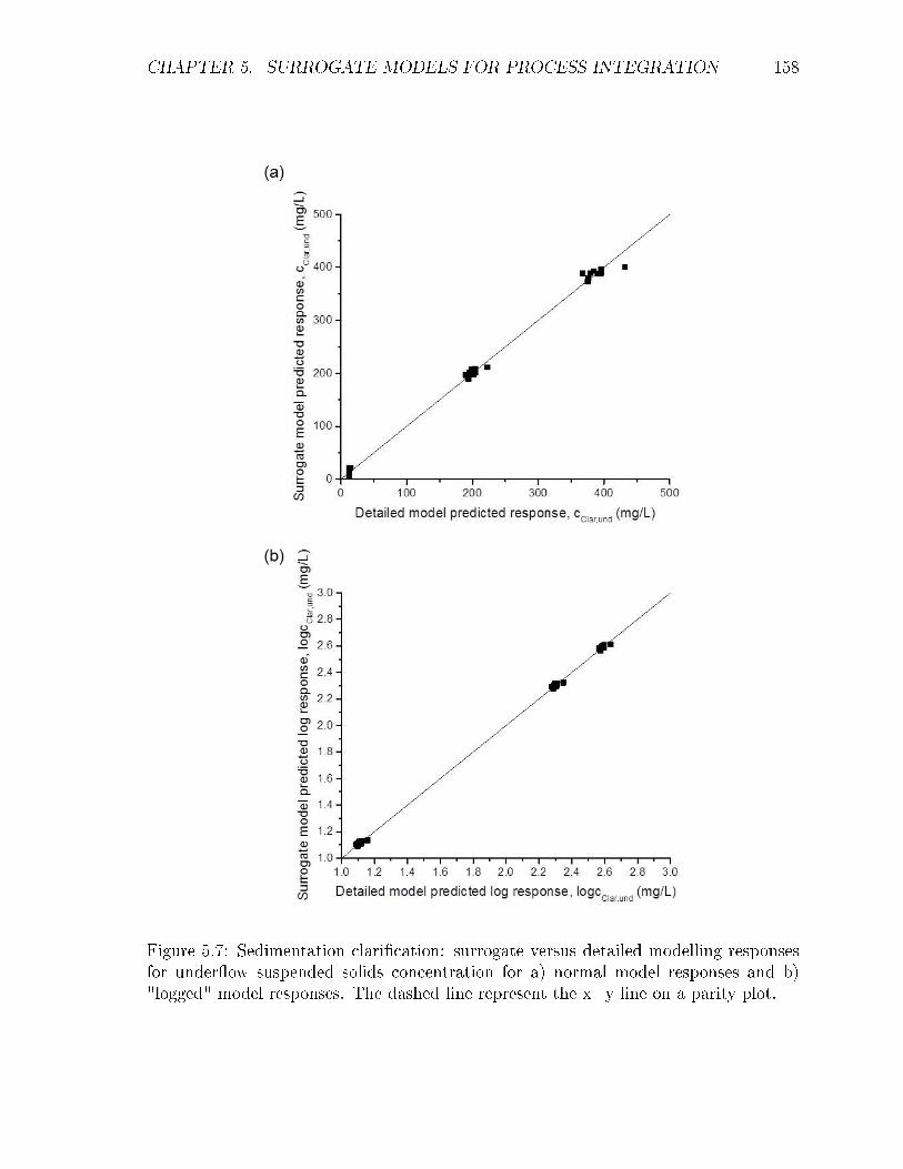
CHAPTER 5. SURROGATE MODELS FOR PROCESS INTEGRATION 158
Figure 5.7: Sedimentation clari�cation: surrogate versus detailed modelling responsesfor under�ow suspended solids concentration for a) normal model responses and b)"logged" model responses. The dashed line represent the x=y line on a parity plot.

CHAPTER 5. SURROGATE MODELS FOR PROCESS INTEGRATION 159
Table 5.10: Veri�cation of e�uent suspended solids concentration derived from "logged"and "unlogged" surrogate model for clari�cation via sedimentation against the detailedmodel.
Normal LOG
Run c0
(mg/L)
Qf
(m3/s)
Lf
(m)
DetailedcFloc,COM
(mg/L)
SurrogatecFloc,COM
(mg/L)
Error
%
DetailedcFloc,COM
(mg/L)
SurrogatecFloc,COM
(mg/L)
Error
%
Inside prediction range (5 ≤ c0 ≤ 150, 0.0064 ≤ Qf ≤ 0.1, and 1 ≤ Lf ≤ 3)
1 80 0.0875 1 0.48 0.55 13 -0.32 -0.33 2.58
2 40 0.069 1.5 0.058 -0.059 3.51 -1.24 -1.77 43.3
3 10 0.078 2 0.0024 0.17 6796.8 -2.61 -2.83 8.14
4 140 0.097 2.5 0.033 -0.145 338.7 -1.48 -1.64 10.4
Outside prediction range (c0 < 5, c0 > 150, Qf < 0.0064, Qf > 0.1, and Lf < 1, Lf > 3)
5 4 0.056 -0.5 0.043 0.23 442 -1.37 -1.02 25.03
6 4 0.056 1 0.0046 -0.22 4624 -2.34 -2.21 5.48
7 4 0.063 1 0.0072 -0.27 3674 -2.14 -2.03 5.2
8 140 0.14 -0.75 5.92 9.42 59.2 0.77 0.82 6.72
9 120 0.07 0 2.09 2.11 0.91 0.32 0.39 20.8
10 170 0.11 -0.25 5.43 6.45 18.5 0.74 0.74 0.49
solids concentration using the surrogate model against the under�ow suspended solids
concentration determined by the detailed model. For both the "logged" and "unlogged"
versions of the model, the surrogate models show a strong linear trend; however, the
data points cluster up in three speci�c areas and this is associated with whether the
initial suspended solids concentration has been given a low, centre or high numerical
number. This is a re�ection of industrial water treatment practices, as it is expected
the under�ow �ow suspended solids concentration will have the highest concentration
of suspended solids which is due for removal via a sludge collector (Jeppsson and Diehl,
1996; Ramin et al., 2014). The R2 value suggests that although both models might
provide accurate predictions. Moreover, the model �tted to "logged" data is more
slightly accurate along the desired operating range (R2log= 99.9% and R2
unlog= 99.6%).
Figure 5.7 show that the surrogate models are able to predict the phenomena from
the detailed model. Figure 5.6 represents graphically the range in which the surrogate
model will be �tted and Table 5.11 provides the data for the veri�cation of the surrogate
model. Inside of the prediction range, the four runs show that the "unlogged" surrogate
model generally produces a smaller error when compared with the detailed model (run 1
- 3: 0.72% - 19.6%); when compared with the "logged" model there is a larger error (run
1 - 3: 0.35% - 13.8%). There is a large error predicted for run 4 for both the �logged�
and �unlogged� model, the three variables c0, Qf and Lf are near the upper boundary

CHAPTER 5. SURROGATE MODELS FOR PROCESS INTEGRATION 160
Table 5.11: Veri�cation of under�ow suspended solids concentration derived from"logged" and "unlogged" surrogate model for clari�cation via sedimentation againstthe detailed model.
Normal LOG
Run c0
(mg/L)
Qf
(m3/s)
Lf
(m)
DetailedcFloc,COM
(mg/L)
SurrogatecFloc,COM
(mg/L)
Error
%
DetailedcFloc,COM
(mg/L)
SurrogatecFloc,COM
(mg/L)
Error
%
Inside prediction range (5 ≤ c0 ≤ 150, 0.0064 ≤ Qf ≤ 0.1, and 1 ≤ Lf ≤ 3)
1 80 0.0875 1 217 215.4 0.72 2.34 2.34 0.35
2 40 0.069 1.5 102 105.9 3.88 2 1.8 10.3
3 10 0.078 2 25 20 19.6 1.4 1.2 13.8
4 140 0.097 2.5 61 346.6 467.7 1.79 2.57 44
Outside prediction range (c0 < 5, c0 > 150, Qf < 0.0064, Qf > 0.1, and Lf < 1, Lf > 3)
5 4 0.056 -0.5 9.9 1.32 86.7 0.99 1.07 7.4
6 4 0.056 1 10.2 19.4 89.9 1.01 1.1 9.28
7 4 0.063 1 10.3 18.5 80 1.01 1.1 8.9
8 140 0.14 -0.75 248.6 336 35.2 2.4 2.5 5.34
9 120 0.07 0 317 310.3 1.9 2.5 2.57 3.14
10 170 0.11 -0.25 352 435 23.7 2.51 2.5 2.5
within the desired range; however, Figure 5.7 shows the linear �t and predicted response
will lay in an area that has no predicted points near it. This shows a limitation of this
surrogate model.
With the R2 value for the "logged" model being 99.9%, it can be interpreted as the
"logged" model is a better �t; however, further investigation shows that it is not as
accurate within the desired range. There are six runs simulated for outside of the
prediction range (with the same values as explained for the model above) to see how both
the detailed and surrogate models will react when faced with a variety of variables both
inside and outside of the desired ranges. These six runs are in agreement the �ndings
within the desired range and shows that the "unlogged" model is able to accurately
predict the values when the initial suspended solid concentration and inlet volumetric
�ow rate are within the desired range.
5.4.2 Concluding remarks
The primary objective of this study is the development of surrogate models (from
detailed models developed in Chapter 3), for the clari�cation unit, which are able to
accurately predict the e�uent suspended solids concentration. For the clari�cation via

CHAPTER 5. SURROGATE MODELS FOR PROCESS INTEGRATION 161
sedimentation, two responses are predicted; the e�uent suspended solids concentration,
cClar,eff , and the under�ow suspended solids concentration, cClar,und. The surrogate
models can be used in either a "logged" or "unlogged" form and eventhough the R2
coe�cients were close for both alternatives, the numerical errors during the veri�c-
ation revealed which for was the best to use. For predicting the e�uent suspended
solids concentration, cClar,eff , there is a discrepancy between the R2 coe�cient for the
"logged" and "unlogged" model with the "logged" data being closer to one, where R2
of one indicates the regression line perfectly �ts the data. As shown in Figure 5.7, the
"logged" model has a stronger linear �t and from analysing the model sensitivities with
the numerical values inside and outside of the desired ranges, it was recon�rmed that
the "logged" model is the more accurate model to use as the absolute errors between the
surrogate model prediction and the detailed model response was smaller. For predicting
the under�ow suspended solids concentration, cClar,und, the "logged" and "unlogged"
model produced a similar R2 values, despite the grouping of the responses into three
distinct regions (low, centre and high). By logging the response of the detailed model,
there is an increase in the models predictive capacity, due to the highly linear correlation
and the predicted values �t very closely to the detailed model values. The surrogate
model for predicting the under�ow suspended solids concentration, cClar,und, will be the
models based on "logged" data.
5.5 Filtration surrogate model
In Chapter 3, one detailed mathematical model is developed to represent the rapid
gravity �ltration process unit for the �ltration processing step.
Rapid gravity �ltration
In this section, a surrogate model will be developed which links three key variables
to the e�uent suspended solids concentration at the �ltration breakthrough stage.
This is a�ected by the initial suspended solids concentration, the �ltration velocity
and the depth of the unit. This model simpli�cation allows for easier optimisation of
the complete conventional clean water treatment process. Using Equation 5.2.2, the
polynomial equation will take on the form:

CHAPTER 5. SURROGATE MODELS FOR PROCESS INTEGRATION 162
cFil = β0 + β1x1 + β2x2 + β3x3 + β11x21 + β22x
22 + β33x
23
+β12x1x2 + β13x1x3 + β23x2x3
(5.5.1)
where
cFil e�uent suspended solids concentration, (mg/L)
x1 normalised initial suspended solids, (mg/L)
x2 normalised �ltration velocity (m/s)
x3 normalised �lter bed depth, (m)
The three factors, x1, x2 and x3will be explored at three di�erent levels (low, centre and
high) with the goal of �nding an average desirability range. By using Equation 5.2.5,
the following will be used to determine the factors for each variable:
x1 =
[c0 − c0centre
c0centre − c0low
](5.5.2)
x2 =
[u− ucentreucentre − ulow
](5.5.3)
x3 =
[L− LcentreLcentre − Llow
](5.5.4)
where
c0 initial suspended solids, (mg/L)
u �ltration velocity (m/s)
L �lter bed depth, (m)
Utilising the methodology detailed in Section 5.2.2, 27 simulations are needed in order
to have all combinations. Table 5.12 presents the typical ranges of operation that were
considered to ensure the level of accuracy, and the justi�cations for the choices.
Once these variables are set values, the detailed models are simulated with the di�erent
combinations of variable values to obtain an e�uent suspended solids concentration.
Microsoft Excel is then utilised to develop the surrogate models from steps 2 to 7.
Table 5.13 presents the numerical values for the least squares estimator, β, for the
e�uent suspended solids concentration leaving �ltration unit. The regression equation
developed for the "unlogged" and "logged" values of cFil are:
cfil = 0.129 + 0.136x1 + 0.444x2 − 0.16x3 − 0.018x21 − 0.011x2
2
+0.0948x23 + 0.0392x1x2 − 0.138x1x3 − 0.0297x2x3
(5.5.5)
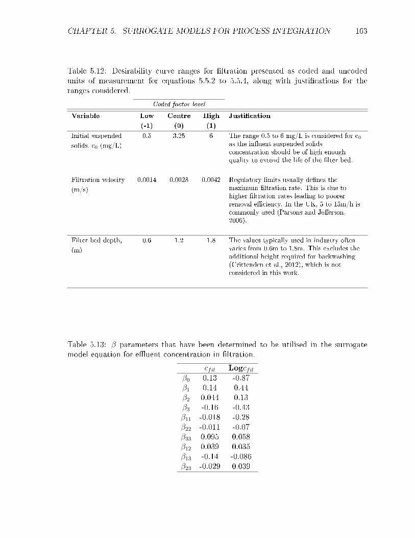
CHAPTER 5. SURROGATE MODELS FOR PROCESS INTEGRATION 163
Table 5.12: Desirability curve ranges for �ltration presented as coded and uncodedunits of measurement for equations 5.5.2 to 5.5.4, along with justi�cations for theranges considered.
Coded factor level
Variable Low
(-1)
Centre
(0)
High
(1)
Justi�cation
Initial suspended
solids, c0 (mg/L)
0.5 3.25 6 The range 0.5 to 6 mg/L is considered for c0as the in�uent suspended solidsconcentration should be of high enoughquality to extend the life of the �lter bed.
Filtration velocity
(m/s)
0.0014 0.0028 0.0042 Regulatory limits usually de�nes themaximum �ltration rate. This is due tohigher �ltration rates leading to poorerremoval e�ciency. In the UK, 5 to 15m/h iscommonly used (Parsons and Je�erson,2006).
Filter bed depth,
(m)
0.6 1.2 1.8 The values typically used in industry oftenvaries from 0.6m to 1.8m. This excludes theadditional height required for backwashing(Crittenden et al., 2012), which is notconsidered in this work.
Table 5.13: β parameters that have been determined to be utilised in the surrogatemodel equation for e�uent concentration in �ltration.
cfil Logcfilβ0 0.13 -0.87β1 0.14 0.44β2 0.044 0.13β3 -0.16 -0.43β11 -0.018 -0.28β22 -0.011 -0.07β33 0.095 0.058β12 0.039 0.035β13 -0.14 -0.086β23 -0.029 0.039

CHAPTER 5. SURROGATE MODELS FOR PROCESS INTEGRATION 164
logcfil = −0.867 + 0.436x1 + 0.132x2 − 0.43x3 − 0.284x21 − 0.071x2
2
+0.058x23 + 0.0355x1x2 − 0.0857x1x3 + 0.0391x2x3
(5.5.6)
The validation and sensitivity analysis of the equations above to predict the e�uent
concentration, cFil, will be presented in Section 5.5.1.
5.5.1 Results and validation
In this section, the surrogate model developed for the rapid gravity �ltration unit is
veri�ed and the response values are analysed. The R2 shows the "logged" model has a
better �t than the "logged" model with values of 99.7% and 96.8%, respectively.
Figure 5.8 presents the predicted response for the e�uent suspended solids concen-
tration using the surrogate model against the e�uent suspended solids concentration
determined by the detailed model. For both the "logged" and "unlogged" model, the
surrogate model's predictive capacity seem to be a very good �t as shown by the graphs;
however, the graph for the "logged" data is more linear. The R2 value suggests that
although both models might provide accurate predictions, the model �tted to "logged"
data is more accurate as the "unlogged" data has a cluster of data points at the lower
level of suspended solids concentration (as shown in Figure 5.8).
The models were veri�ed with variable values inside and outside of the ranges considered
in Table 5.12. Figure 5.9 represents graphically the range in which the surrogate model
will be �tted. Table 5.14 provides the data for the veri�cation of the surrogate model.
Inside of the prediction range, the four runs show that generally the "logged" surrogate
model predicts a smaller error when compared with the detailed model response and
this is in agreement with the R2 coe�cient value that shows the "unlogged" data to
have a weaker �t.
There are six runs simulated for outside of the prediction range to see how the models
will react when faced with a variety of variables both inside and outside of the desired
ranges:
� Run 5: None of the variables are within the desired range.
� Run 6: one variable (�lter bed depth, L) is within the desired range whilst two
variables (initial suspended solids concentration, c0, and �ltration velocity, u) are
outside of the range.
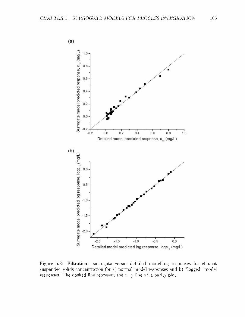
CHAPTER 5. SURROGATE MODELS FOR PROCESS INTEGRATION 165
Figure 5.8: Filtration: surrogate versus detailed modelling responses for e�uentsuspended solids concentration for a) normal model responses and b) "logged" modelresponses. The dashed line represent the x=y line on a parity plot.

CHAPTER 5. SURROGATE MODELS FOR PROCESS INTEGRATION 166
Figure 5.9: Filtration: 3D graphical domain representation of the ranges for the runswithin the ranges (blue dots) and outside of the ranges (black dots) and the data usedfor veri�cation in Table 5.14.
� Run 7: two variables (�lter bed depth, L, and �ltration velocity, u) are within
the desired range whilst one variable (initial suspended solids concentration, c0)
is outside of the range.
� Run 8: None of the variables are within the desired range.
� Run 9: one variable (initial suspended solids concentration, c0) is within the
desired range whilst two variables (�ltration velocity, u and �lter bed depth, L)
are outside of the range.
� Run 10: two variables (initial suspended solids concentration, c0 and �ltration
velocity, u) are within the desired range whilst one variable (�lter bed depth, L)
is outside of the range.
This sensitivity study further shows that the "unlogged" model is not accurate enough
and has a poor prediction of values inside and outside of the desired range. The "logged"
model has a slight under prediction of the e�uent suspended solids concentration
and although these values are small, the �ltration unit itself has very low e�uent
concentration so a small error is signi�cant.

CHAPTER 5. SURROGATE MODELS FOR PROCESS INTEGRATION 167
Table 5.14: Veri�cation of e�uent suspended solids concentration derived from "logged"and "unlogged" surrogate model for �ltration via rapid gravity �ltration against detailedmodels.
Normal LOG
Run c0
(mg/L)
Qf
(m3/s)
Lf
(m)
DetailedcFloc,COM
(mg/L)
SurrogatecFloc,COM
(mg/L)
Error
%
DetailedcFloc,COM
(mg/L)
SurrogatecFloc,COM
(mg/L)
Error
%
Inside prediction range (0.5 ≤ c0 ≤ 6, 0.0014 ≤ u ≤ 0.0042, and 0.6 ≤ L ≤ 1.8)
1 0.6 0.0028 0.9 0.04 0.019 50.1 -1.39 -1.36 2.14
2 4 0.0022 1.2 0.13 0.14 6.19 -0.88 -0.84 4.16
3 2 0.00375 1.6 0.06 0.04 32.4 -1.23 -1.29 5.7
4 5 0.0017 0.6 0.44 0.47 6.2 -0.35 -0.31 -15.8
Outside prediction range (c0 < 0.5, c0 > 6, u < 0.0014, u > 0.0042, and L < 0.6, L > 1.8)
5 0.3 0.0011 0.5 0.039 0.047 17.2 -1.39 -1.35 -3.48
6 0.3 0.0011 0.7 0.023 -0.009 62.1 -1.64 -1.52 7.46
7 0.3 0.0013 0.7 0.029 0.0016 94.7 -1.53 -1.47 3.44
8 6.5 0.0044 2 0.075 0.05 38.2 -1.13 -1.19 5.4
9 1 0.0047 0.2 0.23 0.29 27.2 -0.64 -0.9 40.3
10 3 0.003 2.5 0.03 0.24 816 -1.59 -1.5 4.26
5.5.2 Concluding remarks
The primary objective of this study in this section was the development of surrogate
models for the �ltration unit, which are able to accurately predict the e�uent suspended
solids concentration. The "logged" model provides the most accurate �t and is able
to represent the mechanistic phenomena of breakthrough. Eventhough there is a slight
�uctuation of over and under predicting the e�uent suspended solid concentration
errors are small, thus enabling the use of this model.
5.6 Disinfection surrogate model
Disinfection of clean water prior to release to customers is most commonly accomplished
by the use of either chemical agents (such as chlorine and ozone) or physical agents
(such as light and heat). In the literature, there are many empirical models available
for a variety of disinfection models that can be utilised as simple surrogate models as
described in Chapter 2. In this section, three disinfection processes: chlorine dioxide,
ozonation and ultraviolet light (UV), will be explored. Chlorination is another common
disinfection process but as it is ine�ective in the inactivation of Cryptosporidium, and
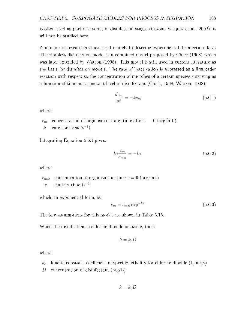
CHAPTER 5. SURROGATE MODELS FOR PROCESS INTEGRATION 168
is often used as part of a series of disinfection stages (Corona-Vasquez et al., 2002), it
will not be studied here.
A number of researchers have used models to describe experimental disinfection data.
The simplest disinfection model is a combined model proposed by Chick (1908) which
was later extended by Watson (1908). This model is still used in current literature as
the basis for disinfection models. The rate of inactivation is expressed as a �rst order
reaction with respect to the concentration of microbes of a certain species surviving as
a function of time at a constant level of disinfectant (Chick, 1908; Watson, 1908):
dcmdt
= −kcm (5.6.1)
where
cm concentration of organisms at any time after t = 0 (org/mL)
k rate constant (s−1)
Integrating Equation 5.6.1 gives:
lncmcm,0
= −kτ (5.6.2)
where
cm,0 concentration of organisms at time t = 0 (org/mL)
τ contact time (s−1)
which, in exponential form, is:
cm = cm,0 exp−kτ (5.6.3)
The key assumptions for this model are shown in Table 5.15.
When the disinfectant is chlorine dioxide or ozone, then:
k = kcD
where
kc kinetic constant, coe�cient of speci�c lethality for chlorine dioxide (L/mg,s)
D concentration of disinfectant (mg/L)
k = koD

CHAPTER 5. SURROGATE MODELS FOR PROCESS INTEGRATION 169
Table 5.15: Assumptions and comments for the disinfection model development.
Assumption Justi�cation
Chick's law holds for ideal
conditions.
All cells of a single species are equally susceptible to thedisinfectants (Chick, 1908).
Contact tank may be modelled
as a continuously stirred tank
reactor.
Concentration of disinfectant and the water matrix remainsconstant through the contact period.
Cells and the disinfectant are
uniformly dispersed in water.
The di�erence between the experimental lab scale predicted Dτ*value and the scaled up actual required Dτ* will only be a�ectedby dispersion a little bit according to Crittenden et al. (2012).
3-log** (99.9% inactivation) are
required for organism reduction.
Raw water sources for wastewater contains a large amount ofbacteria whilse clean water treatment raw water sources containconsiderably less. In practise, �ltration removes majority of theorganism (Crittenden et al., 2012), which is not modelled in thiswork as more data is needed.
No residual decay of
disinfectant.
Constant disinfectant concentration is able to be maintained atlab scale.
*Dτ is a parameter established by Chick (1908) and Watson (1908), where they provided a database
of extensive values.
**Log inactivation is a convenient way to express the number or percentage of microorganisms
inactivated (killed or unable to replicate) through the disinfection process.
where
ko kinetic constant, coe�cient of speci�c lethality for ozone (L/mg,s)
When the disinfectant is UV, then:
k = kUV I
where
kUV kinetic constant, a function of transmittance (cm2/J,s)
I intensity of UV radiation (W/m2)
To determine the kinetic constants, kc, ko, kUV , for a given level of survival (CmCm,0
), where
log removal/inactivation relates to the % removal/inactivation of microorganisms, such
that:
� 1-log reduction = 9 out of 10 = 90% reduction

CHAPTER 5. SURROGATE MODELS FOR PROCESS INTEGRATION 170
� 2-log reduction = 99 out of 100 = 99% reduction
� 3-log reduction = 999 out of 1,000 = 99.9% reduction
� 4-log reduction = 9,999 out of 10,000 = 99.99% reduction
Therefore rearranging Equation 5.6.2 and taking chlorine dioxide and a 1-log reduction
as an example, then:
kc =ln(0.1)
Dτ(5.6.4)
when Dτ is known (Chick, 1908; Watson, 1908).
Relationship between suspended solids concentration and microorganism
concentration
Suspended solid particles form a great challenge for inactivating microorganisms. Sus-
pended solids concentration is usually associated with the aesthetics of the water but
there are some speci�c health concerns with the interaction between suspended solids
concentration and microorganisms. Montgomery (1985) states that one of the speci�c
health-related characteristics of suspended solids (turbidity) was the association of mi-
croorganisms with particulate material, with a resulting interference with disinfection.
Particles a�ect the disinfection process in two distinct ways: 1) particles can react with
the chemical disinfectant or can absorb the UV light, and 2) microorganisms can be
embedded in the particles, shielding them from disinfection. Currently, there is limited
information on e�ective methods for quantifying particle-associated microorganisms
(Montgomery, 1985; Hendricks, 2006; Crittenden et al., 2012), and this brings much
uncertainty into quantifying the impact of particle association on disinfection. Scheible
(1987) modi�es Equation 5.6.5 to account for suspended solid particles acting as an
inactivation hindrance. The author proposed a sub-division of the entire microorganism
load in water into two categories: microorganisms that are accessible, and can therefore
be inactivated, and microorganisms associated with suspended particles and therefore
not able to be inactivated easily. This subdivision of microorganisms into two groups
led to the following expression of inactivation kinetics:
cm =(c′
m,0 + cm,p
)exp (−kτ) + cm,p (5.6.5)
where c'm,0 is the initial concentration of microorganisms accessible per unit volume
of water (org/mL) and cm,p is the concentration of microorganisms (associated with
suspended solid particles) per unit volume of water to disinfection (org/mL).
CHAPTER 5. SURROGATE MODELS FOR PROCESS INTEGRATION 171
Scheible (1987) also states that the value of c′m,0 is larger than the value of cm,p, so it
can be assumed that the total initial microorganism concentration, cm,0, is equal to c′m,0
+ cm,p. Equation 5.6.5 can now be written as an improved version of Equation 5.6.3:
cm = cm,0 exp (−kτ) + cm,p (5.6.6)
It can be seen from the equation that a residual concentration of microorganisms
cm,p persist in water, whatever the amount of disinfection applied. The persistence
of Giardia and Cryptosporidium is a concern because of the di�culty in inactivating
these microorganisms and they are a particularly dangerous protozoa that can cause a
non-treatable form of diarrhoea (Directive, 1998; World Health Organisation, 2011). By
ensuring their removal, most other organisms may also be removed. The research work
of LeChevallier and Norton (1992) examines the relationship between particle count
and Giardia, Cryptosporidium and suspended solids concentration (turbidity).
LeChevallier and Norton (1992) develop a "logged" polynomial regression model for the
determination of the residual number of microorganisms cm,p due to suspended solids
concentration interference:
Giardialogcm,p = 0.664(logcss) + 0.717
linear regression 0.879(5.6.7)
Cryptosporidium
logcm,p = 0.66(logcss) + 0.488
linear regression 0.83(5.6.8)
where
css concentration of suspended solids in water (mg/L)
A number of case studies for Equation 5.6.6 will be conducted to evaluate these models.
Since this equation is a simple empirical equation, there is no need to develop surrogate
models as there is no additional computational advantage in doing so.
5.6.1 Results and validation
For the two following case studies, Table 5.16 presents the typical ranges of operation
and the justi�cations for the choices.

CHAPTER 5. SURROGATE MODELS FOR PROCESS INTEGRATION 172
Table 5.16: Parameters ranges for disinfection units considered.
Variable Symbol Disinfection Range Justi�cation
Concentration of
disinfectant
D (mg/L)Chlorine dioxide 0.2 - 1.5 Typical ranges for
the dosages
(Crittenden et al.,
2012)
Ozone 1 - 5
I (W/cm2) Ultraviolet light 20-100
Contact time τ (s−1)
Chlorine dioxide 600 - 1800 Typical ranges forthe contact time(LeChevallier andAu, 2004)
Ozone 300 - 600
Ultraviolet light 120 - 600
Table 5.17: Values used for disinfection model development in the inactivation ofGiardia for 3-log inactivation (99.9%) (Environmental Protection Agency, 2003a).
Disinfectant Dτ k Conditions
Chlorine dioxide 900 (mg/L,s) 0.00768 (L/mg,s) T =20oC, pH = 6 - 7
Ozone 43.2 (mg/L,s) 0.159 (L/mg,s) T =20oC, pH = 6 - 7
Ultraviolet light 2160 (W/cm2,s) 0.00319 (cm2/W,s)
Giardia
In this section, the predicted microorganism inactivation of Giardia via chlorine dioxide,
ozonation and ultraviolet light using Equation 5.6.6 is tested. In this model, the rate of
inactivation of a microorganism is dependent on the concentration of the disinfectant
and contact time. For this case study, it is assumed that the raw water entering this
unit contains 10,000 org/L of microorganism, the suspended solids concentration is
0.05 mg/L and that a 3-log inactivation is su�cient to remove the Giardia oocysts
(Edzwald, 2011) in order to meet the water quality regulations of negligible (zero)
microogranisms should be present prior to distribution (World Health Organisation,
2011). Table 5.17 presents the values which will be used to determine the e�uent
microorganism concentration.
The empirical equations for the determination of the concentration of microorganims
after disinfection cm are:
For chlorine dioxide:
cm = cm,0exp−0.00768Dτ + exp0.664(logcss)+0.717 (5.6.9)

CHAPTER 5. SURROGATE MODELS FOR PROCESS INTEGRATION 173
For ozone:
cm = cm,0exp−0.159Dτ + exp0.664(logcss)+0.717 (5.6.10)
For ultraviolet light:
cm = cm,0exp−0.00319Iτ + exp0.664(logcss)+0.717 (5.6.11)
In the regression models, coded variables are used of three levels: low, centre and high
which corresponds to speci�c numerical values from the ranges shown in Table 5.16 and
graphically in Figure 5.10. Table 5.18 provides the responses when comparing all the
possible combinations. Equation 5.6.6 includes the concentration of microorganisms
associated with suspended solid particles, cm,p. For clarity in the inactivation power
of the di�erent disinfectants, the responses reported in the table for concentration of
microorganisms after disinfection cm are presented without the addition of cm,p, which is
calculated to be 0.28 mg/L. Table 5.18 also shows the concentration of microorganisms
after disinfection cm for chlorine dioxide, ozone and UV disinfectants.
The values of cm show that for the disinfection of Giardia, ozone is the most e�cient at
the inactivation of the microorganism and chlorine dioxide is the least e�cient; this is
consistent with experimental �ndings in the literature (Crittenden et al., 2012). Within
the disinfectant concentration and contact time ranges for the three di�erent options,
it can be seen that using chlorine dioxide for the inactivation of Giardia requires the
highest dose (1.5 mg/L) and contact time (1800 s−1) is needed to obtain a cm within
the required purity regulation (World Health Organisation, 2011). The smallest contact
time (600 s−1) for chlorine dioxide has a big e�ect on the inactivation as it can be
seen in the table, for the three doses (0.2 mg/L, 0.85 mg/L and 1.5 mg/L) with this
contact time, that the microorganism concentration will never meet the required purity
standards. The lowest value given for chlorine dioxide is 1×10⁻⁵ org/mL; even though
this is a small number, it is still quite a larger amount of Giardia oocysts left meaning
that chlorine dioxide might not be suitable for this inactivation. Disinfection with ozone
follows a similar trend to the chlorine dioxide where the higher dose concentration
and contact time result in higher inactivation thus, demonstrating that an optimal
performance criteria can be determined when taking the desired ranges into account.
The predicted inactivation by ultraviolet light is more promising as, even though the
largest inactivation occurred with the highest dose concentration and contact time,
Runs 6 and 8 cm predictions are same value for di�erent doses and contact time. Taking
this into account, reveals that for a dose of 60 W/cm2 and a contact time of 600 s−1 or

CHAPTER 5. SURROGATE MODELS FOR PROCESS INTEGRATION 174
Figure 5.10: Disinfection: 2D graphical domain representation of the ranges for theruns and the data used for veri�cation in Table 5.18 , where represented in a) chlorinedioxide range b) ozone range and c) ultraviolet light range.

CHAPTER 5. SURROGATE MODELS FOR PROCESS INTEGRATION 175
Table 5.18: Model test results in the prediction of e�uent microorganism concentrationfrom Equations 5.6.9, 5.6.10, and 5.6.11 for inactivation of Giardia via disinfection usingchlorine dioxide, ozone and ultraviolet light.
Chlorine Dioxide
Run Disinfection
Concentration, D
(mg/L)
Contact time, τ (s−1) cm (org/L)
1 0.2 600 3981.1
2 0.2 1200 1584.9
3 0.2 1800 630.9
4 0.85 600 199.5
5 0.85 1200 3.98
6 0.85 1800 0.079
7 1.5 600 10
8 1.5 1200 0.01
9 1.5 1800 1×10⁻⁵
Ozone
Run Disinfection
Concentration, D
(mg/L)
Contact time, τ (s−1) cm (org/L)
1 1 300 1.47×10⁻¹⁷
2 1 450 5.62×10⁻²⁸
3 1 600 2.15×10−38
4 3 300 3.16×10−59
5 3 450 1.78×10−90
6 3 600 1×10−121
7 5 300 6.81×10−101
8 5 450 5.62×10−153
9 5 600 4.64×10−205
Ultraviolet light
Run Disinfection
Concentration, I
(W/cm2)
Contact time, τ (s−1) cm (org/L)
1 20 120 4.64
2 20 360 1×10⁻⁶
3 20 600 2.15×10⁻¹³
4 60 120 1×10⁻⁶
5 60 360 1×10⁻²⁶
6 60 600 1×10−46
7 100 120 2.15×10⁻¹³
8 100 360 1×10−46
9 100 600 4.64×10−80
Please note: the small values are here for comparison purposes, in reality they are not measurable
and will equal zero as the standard requires (World Health Organisation, 2011).

CHAPTER 5. SURROGATE MODELS FOR PROCESS INTEGRATION 176
a dose of 100 W/cm2 and a contact time of 360 s−1 will give a e�uent microorganism
concentration of 1×10−46 (negligible) so a cost trade o� can be conducted to determine,
which variable can be manipulated to �nd an optimal performance criteria.
Cryptosporidium
In this section, the predicted microorganism inactivation of Cryptosporidium via chlor-
ine dioxide, ozonation and ultraviolet light using Equation 5.6.6 is tested. In this
model, the rate of inactivation of a microorganism is dependent upon the concentration
of the disinfectant and contact time. For this case study, it is assumed that the
raw water entering this unit contains 10,000 org/L of microorganism, the suspended
solids concentration is 0.05 mg/L and that a 2-log inactivation is su�cient enough to
remove the Cryptosporidium oocysts (Edzwald, 2011) in order to meet the water quality
regulations of negligible (zero) microorganisms should be present prior to distribution
(World Health Organisation, 2011). Table 5.19 presents the values which will be used
to determine the e�uent microorganism concentration. The empirical equation for the
determination of the concentration of microorganism after disinfection cm are:
For chlorine dioxide:
cm = cm,0exp−3.29e−5Dτ + exp0.66(logcss)+0.488 (5.6.12)
For ozone:
cm = cm,0exp−0.00984Dτ + exp0.66(logcss)+0.488 (5.6.13)
For ultraviolet light:
cm = cm,0exp−0.00794Iτ + exp0.66(logcss)+0.488 (5.6.14)
In the regression models, coded variables are used of three levels: low, centre and high
which corresponds to speci�c numerical values from the ranges shown in Table 5.16
and graphically in Figure 5.10. Table 5.20 provides the responses when comparing
all the possible combinations. In line with the same reasoning as earlier, for clarity
in the inactivation power of the di�erent disinfectants, the responses reported in the
table for concentration of microorganisms after disinfection cm are presented without
the addition of cm,p, which is calculated to be 0.28 mg/L.

CHAPTER 5. SURROGATE MODELS FOR PROCESS INTEGRATION 177
Table 5.19: Values used for disinfection model development in the inactivation ofCryptosporidium for 2-log inactivation (99%) (Environmental Protection Agency,2003b).
Disinfectant Dτ k Conditions
Chlorine dioxide 139,920 (mg/L,s) 3.29e−5 (L/mg,s) T =20oC, pH = 6 - 7
Ozone 468 (mg/L,s 0.00984 (L/mg,s) T =20oC, pH = 6 - 7
Ultraviolet light 10 (W/cm2,s) 0.794 (cm2/W,s)
Table 5.20 shows that chlorine dioxide is ine�ective in the inactivation of the Crypto-
sporidium oocysts, and Binnie and Kimber (2009) suggest use of chlorine dioxide as
a disinfectant may be considered in a series of disinfection processes as one of the
steps. Disinfection with ozone shows it is able to inactivate a large portion of the
Cryptosporidium with the higher dose (5 mg/L) and contact time (500 s−1). However,
the e�uent microorganism predicted is still larger than the predicted concentration
using ultraviolet light at a low dose (20 W/cm2) and medium contact time (360 s−1).
UV is the most e�cient at the inactivation of the microorganism and once again
chlorine dioxide is the least e�cient. This is consistent with experimental �ndings
in the literature (World Health Organisation, 2011; Crittenden et al., 2012; Binnie and
Kimber, 2009). The inactivation by ultraviolet light shows the same correlation with
the Giardia microorganism concentration, in cm predictions for Runs 6 and 8 have the
same value for di�erent doses (60 W/cm2 and 100 W/cm2) and contact time (600 s−1
and 360 s−1, respectively). This gives some scope for optimisation around the variables
in order to �nd an optimal performance criteria.
5.6.2 Concluding remarks
The primary objective of this study was the utilisation of an improved Chick-Watson
empirical model (Equation 5.6.6) that can predict the e�uent microorganism con-
centration after disinfection. This equation takes into account the concentration of
microorganisms that will be a�ected by the presence of suspended solids concentra-
tion that remain in water. Testing the three di�erent disinfection empirical models
within the desired ranges for the inactivation of Giardia revealed that both ozone and
ultraviolet disinfection can be utilised to successfully disinfect the Giardia oocysts.
Ozone is the best form of disinfection whilst chlorine dioxide is not adequate to be used
for this microorganism but could possibly be used as a primary disinfection treatment
followed by a secondary disinfection treatment. For the testing of Cryptosporidium, the
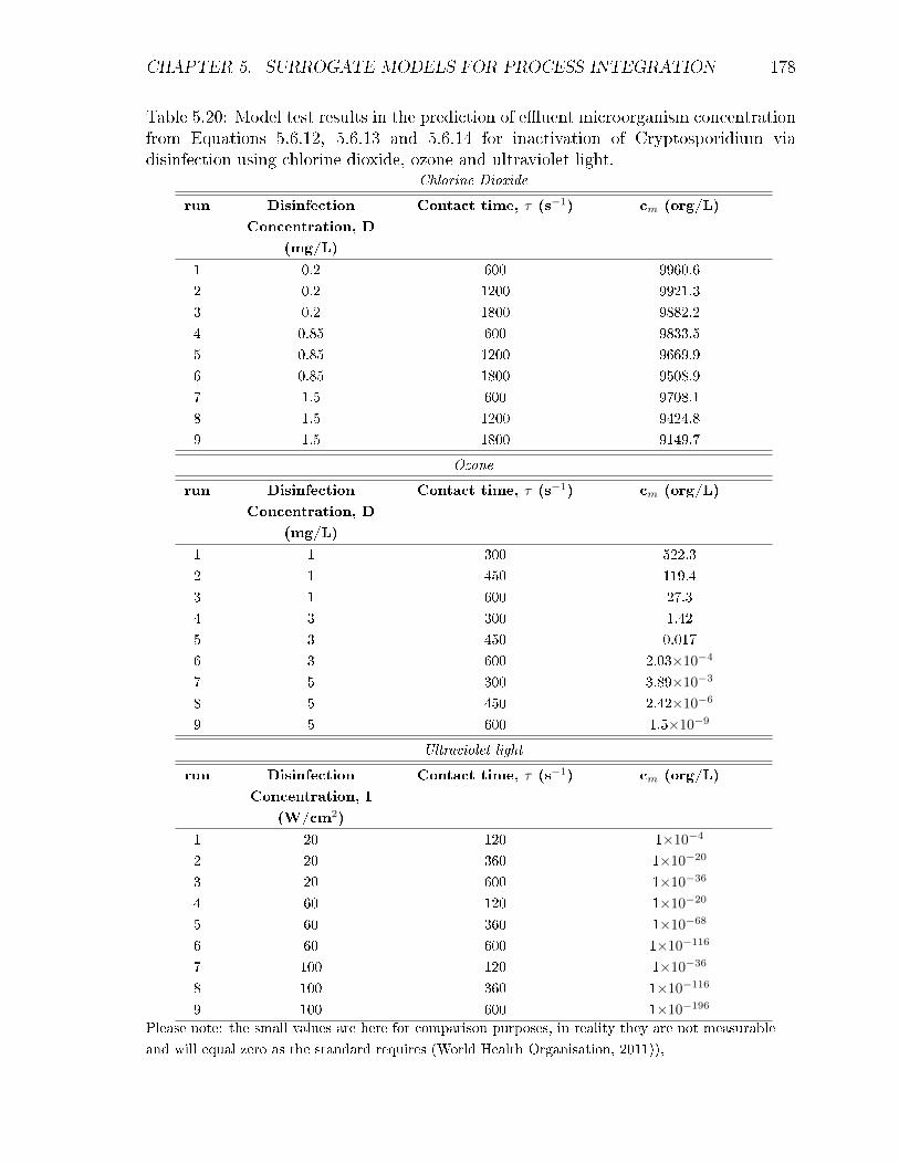
CHAPTER 5. SURROGATE MODELS FOR PROCESS INTEGRATION 178
Table 5.20: Model test results in the prediction of e�uent microorganism concentrationfrom Equations 5.6.12, 5.6.13 and 5.6.14 for inactivation of Cryptosporidium viadisinfection using chlorine dioxide, ozone and ultraviolet light.
Chlorine Dioxide
run Disinfection
Concentration, D
(mg/L)
Contact time, τ (s−1) cm (org/L)
1 0.2 600 9960.6
2 0.2 1200 9921.3
3 0.2 1800 9882.2
4 0.85 600 9833.5
5 0.85 1200 9669.9
6 0.85 1800 9508.9
7 1.5 600 9708.1
8 1.5 1200 9424.8
9 1.5 1800 9149.7
Ozone
run Disinfection
Concentration, D
(mg/L)
Contact time, τ (s−1) cm (org/L)
1 1 300 522.3
2 1 450 119.4
3 1 600 27.3
4 3 300 1.42
5 3 450 0.017
6 3 600 2.03×10⁻⁴
7 5 300 3.89×10⁻³
8 5 450 2.42×10⁻⁶
9 5 600 1.5×10⁻⁹
Ultraviolet light
run Disinfection
Concentration, I
(W/cm2)
Contact time, τ (s−1) cm (org/L)
1 20 120 1×10⁻⁴
2 20 360 1×10⁻²⁰
3 20 600 1×10−36
4 60 120 1×10⁻²⁰
5 60 360 1×10−68
6 60 600 1×10−116
7 100 120 1×10−36
8 100 360 1×10−116
9 100 600 1×10−196
Please note: the small values are here for comparison purposes, in reality they are not measurable
and will equal zero as the standard requires (World Health Organisation, 2011)),

CHAPTER 5. SURROGATE MODELS FOR PROCESS INTEGRATION 179
same trend was shown where both ozone and ultraviolet disinfection can be utilised for
successful inactivation. Ultraviolet light is the best form of disinfection whilst chlorine
dioxide will not be able to work alone and if used, and again will have to be in a series
of disinfection treatment.
5.7 Conclusion
Due to the complex nature of drinking water treatment unit processes, the process mod-
els, where they exist, are often site speci�c. The use of detailed dynamic models can be
computationally expensive and provide more information than necessary for industrial
purposes, such as for overall plant design. Simple surrogate models that encapsulate
the physical phenomena occurring, and which can provide a similarly accurate response,
are of great bene�t to the water industry. In this chapter, surrogate models have been
developed for all the alternative processing units of operation discussed in Chapter 3.
The use of polynomial regression to determine multi-variable polynomial regression
equations used in this study proved to be an extremely valuable tool to analyse data
obtained from detailed mathematical models for the clean water treatment processes
where the characteristics of the water are constantly changing. Following the meth-
odology described in Section 5.2.2 for the detailed models, surrogate models for two
coagulation/�occulation units (rapid mixing and �occulation in compartments), a cla-
ri�cation (sedimentation) and �ltration (rapid gravity �ltration) units were successfully
developed. The results showed that the surrogate models, used in their logarithmic
transformation form enabled visualisation of the data and the percentage errors, when
comparing with the detailed models. The log transformation is a widely used method
to address skewed data.
Three disinfection units, chlorine dioxide, ozonation and ultraviolet light, were con-
sidered for the inactivation of Giardia and Cryptosporidium. These two protozoa
are particularly di�cult to inactive in water (World Health Organisation, 2011), and
thus, ensuring their removal means most other organisms are removed. Simple em-
pirical equations exist in literature (Chick, 1908; Watson, 1908) and these have been
improved to include a correlation incorporating suspended solids concentration interfer-
ence (LeChevallier and Norton, 1992) as this has a minor a�ect on the microorganism
inactivation but should not be ignored when designing the disinfection section. The
closeness of the data points to the x=y lines on the parity plot reinforces the accuracy
of the developed surrogate models and the utilisation of the three level factorial design.
Chapter 6
Conclusions and recommendations
The primary aim of this thesis is to draw upon previous work in the literature
to develop a �rst principles mathematical model of an entire conventional
clean water treatment work . The thesis contains four distinct contributions.
The key outcome of the work is that there are signi�cant advantages to
be gained by the used of detailed and surrogate mathematical models of
the complete conventional clean water treatment works in industry. The
recommendations for future work is to incorporate enterprise wide modelling,
which would bring together the various modelling tools and expert guidance
to enable industrial users to quickly and e�ciently implement the available
models within industrial constraints in order to shift from a reactive industry
to a more proactive one. The key areas discussed that need addressing
are related to the use of simulation tools in clean water treatment, model
calibration and broader recommendations.
6.1 Review of project deliverables
The overall aim of this thesis was to derive fundamental process understanding of
conventional clean water treatment works, when evaluated as an entire process. The
goal was to add to the development of detailed modelling and analysis of the dynamics
of clean water treatment works as a whole, whilst providing a detailed review of the
current state-of-art and utilising processing systems engineering tools.
180

CHAPTER 6. CONCLUSIONS AND RECOMMENDATIONS 181
6.1.1 Critical assessment of the current state-of art
Traditionally, the water industry has been sitting within the civil engineering domain
rather than the chemical engineering domain as the civil engineers took the lead role in
the design of the plants, e.g. creating the layout of the entire system based on traditional
processing units. Due to the increasing pressure for companies to remain competitive in
the national or global marketplace, the search for e�cient methodologies for operational
management and mitigation of risk has led some to consider the use of Process Systems
Engineering (PSE) methods found in the chemical engineering domain, in particular,
detailed modelling from �rst principles and optimisation based on rigorous optimisation
algorithms, which have been highly successful within the chemical industries.
In Chapter 2, the current state-of-art of mathematical modelling in the clean water
treatment industry is assessed, by focusing on detailed mathematical models and op-
timisation techniques. The review shows that process engineering plays a major role,
in not only modelling of the system processes; but also increasing the fundamental
understanding of the phenomena occurring. An integrated approach to modelling and
optimisation has been found in literature to provide a competitive advantage (Larsson
and Skogestad, 2000; Shah, 2005; Charpentier, 2005; Grossmann, 2005; Varma et al.,
2007). An integrated approach can also be a driving force for operational level optim-
isation based on explicit objectives in the development of novel designs. The developed
models can incorporate water quality data to predict the changes in process parameters
by preceding processing steps or how this change in�uences subsequent processing
steps. Chapter 2 provides a critical analysis of current work, which shows that an
understanding of the phenomena of process units will lead to developed understanding
for better process design.
6.1.2 Dynamic modelling of conventional clean water treatment
work
Simulation is a useful tool and Chapter 3 focused on the use of numerical simulation
for the dynamic modelling of unit processes in clean water treatment works. Chapter
3 examined mathematical models of the most common physical water treatment pro-
cesses, namely coagulation/�occulation, clari�cation, and �ltration units, available in
the current literature. The models considered the key factors that a�ected the e�uent
suspended solids concentration for each unit. Via a sensitivity analysis, each individual

CHAPTER 6. CONCLUSIONS AND RECOMMENDATIONS 182
unit was examined and limitations were tested. The results implied that the models
derived were in good agreement with the literature and could predict successfully predict
propagation of change.
There are a few limitations with the implementation of the models developed. Firstly,
ideal conditions are often assumed which will have an e�ect on the predicted concentra-
tion once the units have been combined to make a complete water treatment model. The
individual unit will behaviour in an ideal manner when a change is proposed meaning
the propagation will have limitations. Secondly, due to the nature of the process models,
empirical parameters are needed for accurate simulation of a process on a speci�c site,
which requires experiments or historical data to �nd empirical relationships. Thirdly,
since the existing work on dynamic modelling of water treatment processes considers
these as separate units, there is therefore a lack of a complete understanding as to
how these models �t together into a model of a complete water treatment plant. The
knowledge and understanding from considering the models of the individual units was
used to direct the e�orts in the formulation of a robust complete water treatment plant
model.
In Chapter 4, the individual water treatment models were combined and it was demon-
strated that the models are able to predict the expected response to propagating
changes. Three di�erent scenarios were presented with three alternative clean water
treatment con�gurations. When a change was imposed, there was successful suspended
solids concentration propagation through the clean water treatment simulation. The
modelling approach based on �rst principles was found to be useful for: (1) increasing
the understanding of the process by providing a more informative method for exploring
how di�erent processing units are a�ected by sequential event, and (2) allowing for a
variety of scenarios to be tested out, which can enhance process management such as
the process design stage, depending on the raw water source available. For a model
like this to be fully utilised it needs to be operator friendly and currently the detailed
mathematical models require knowledge on process systems engineering. By using
detailed modelling (especially gPROMS utilised in this work), an advantage gained is
that operation and variations in time can be evaluated in the design; however, the
calculation times will be longer than with simpler surrogate models.

CHAPTER 6. CONCLUSIONS AND RECOMMENDATIONS 183
6.1.3 Surrogate model development of clean water treatment
work
Without knowledge of advanced simulation tools or having a background in process
modelling, the detailed models developed in this work would not be fully utilised
if implemented in the water industry, if utilised at all. These complex models use
fundamental knowledge and are only concerned with the phenomena occurring within
the individual units. Linking these dynamic models together increases the complexity,
which results in detailed integrated models which may be di�cult to calibrate on a water
treatment plant and also potentially di�cult to solve. The idea of simpler surrogate
models, that can be used to predict the e�uent suspended solids concentration given
a number of independent variables, would therefore be of greater value. In Chapter 5,
response surface modelling of the e�uent suspended solids concentration is implemented
via regression analysis using least squares methods. The developed models are second
order polynomials as it has been demonstrated that this order is su�cient to re�ect
the data as the phenomena occurring within the units are represented by the surrogate
models. The models have been developed using the same methodology, where both the
�logged1 � and �unlogged� data are validated against the detailed dynamic models. The
values are provided as both "unlogged" and "logged" due to a log scale making it easy
to compare values that cover a large range. The results imply that the log form of the
models is the most accurate and provide the best �t with the R2 coe�cient being close
to 1. The transformation of the polynomial surface response for the product purity (in
this case the suspended solids concentration) results in simpler surrogate models which
are easier to use for optimisation purposes.
6.1.4 Concluding remarks
From the work presented in this thesis, the mathematical modelling and programming
techniques employed can be widely applied in the advancement of the water industry.
The mathematical modelling approaches have successfully dealt with the integration of
complete water treatment models and provided a proof of concept in the application of
superstructure optimisation techniques.
The surrogate model approach to plant wide superstructure optimisation used in this
work involves four major steps. The preliminary steps (conducted in Chapter 3)
1For ease of interpretation, the logarithmic transformation of models in the text are referred to as�logged � and the regular model notation is referred to as �unlogged�.

CHAPTER 6. CONCLUSIONS AND RECOMMENDATIONS 184
involved development of the detailed mathematical models for the clean water treatment
units. The detailed models once combined needed to be tested for robustness and
sensitivity towards plant wide modelling, in Chapter 4. Finally, once these models were
constructed, the next step involved choosing the surrogate modelling methodology and
the form of the approximate models (conducted in Chapter 5).
The work in this thesis, which not only has developed some novel approaches to
literature problems but also, considered some problems that have not been investigated
before, is a complement to the literature research work on modelling in the clean water
industry.
6.2 Direction for future research
This thesis shows that there are valuable advantages to be gained from the use of
detailed mathematical models of the conventional clean water treatment works in
industry. However, there are still areas of weakness that need to be addressed before
models can be fully integrated in industrial practise. There are still several research
directions that could be considered for future work as the extension of the current
study and in the following section, potential directions for future work related to use of
detailed and surrogate models in industry are discussed.
6.2.1 Use of numerical simulation tools in drinking water treat-
ment
Model enhancement
As mentioned in Chapter 1, the overall aim of this work is to model a complete
conventional clean water treatment work in order to predict situational changes that
may propagate through the system. Since the focus of this project has been the main
physical water treatment processes, a clear direction would be to include chemical
processing steps, such as the chemical coagulant dosing stage before the �occulation
unit.
The current complete water treatment model presented in this work is simpli�ed by
assumptions and does not take into pH parameters important to maintaining a high
CHAPTER 6. CONCLUSIONS AND RECOMMENDATIONS 185
water quality that may vary depending on each process unit. The level of assumptions
will need to be adjusted through the development of the individual plant units. Para-
meters, such as temperature and pH, have a signi�cant e�ect on the treatment process
and �nal water quality; however, more research is needed on how these parameters can
a�ect a deterministic model as current literature focusses on empirical models which
are site speci�c.
In Chapter 2, it was highlighted that, in the absence of satisfactory means for determin-
ing the number concentration, particle mass concentration is often substituted for num-
ber concentration. In some studies (Edzwald and Van Benschoten, 1990; Hannouche
et al., 2011), a linear relation between suspended solids concentration and turbidity
is assumed and suspended solids concentration is replaced by the easy-to-measure
turbidity; however, with the development of a direct correlation based on fundamental
knowledge then the validity of the suspended solids concentration will be strengthened.
The models developed are in terms of concentration and data given is in terms of
turbidity, so for validation purposes either veri�ed correlations presented in literature
will be used to validate this assumption or experiments calculating the mass of the
settled particles and the turbidity measured to generate a correlation will be used.
Plant-wide surrogate modelling
Although the models created in this study are fairly detailed, they do not approach
the full scale of industrial models. The applicability of the surrogate model approach
to industrial-scale models can only be predicted in this study. To better determine the
bene�ts of the surrogate model approach for an industrial-scale clean water treatment
model, more detail must be added to the detailed plant model. Presented in this work,
is the development of individual surrogate models connected to make an overall plant
model for optimisation purposes. An interesting direction for this work would be the
development of a complete plant wide surrogate model in order to compare against a
detailed model. If data is provided, this can also be compared with plant data.
Another direction would be to extend the surrogate model. The approximate models
used in this work were formulated using detailed models. Several other modelling
methodologies and approximate model types could be used in the surrogate model
approach. In this study, no attempt is made to compare these options. Although some
other modelling methodologies and approximate model types were discussed in this
study, a detailed comparison was not performed. More studies on the application of
these di�erent modelling methodologies and approximate model types could give an
indication of which options provide the best results for large-scale optimisation.

CHAPTER 6. CONCLUSIONS AND RECOMMENDATIONS 186
6.2.2 Plant optimisation
For many years, process optimisation has been used extensively in traditional chemical
engineering sectors such as oil and gas, and is a proven approach for gaining maximum
value out of a process (Grossmann and Biegler, 2004). With the increase in alternative
processes readily available for water treatment plants, the selection of the treatment
processes, which is a combination of unit operations, is a task that has not only increased
the importance of early stage decision making, but also increased the complexity in
a company's ability to remain competitive with increasingly stringent water quality
regulations. With the increase in alternative processing steps readily available for clean
water treatment plants, the selection of the individual treatment processes for each
processing step is a task that has not only increased the importance of early stage
decision making, but will also increase the plant's ability to remain competitive with
the increasingly stringent water quality regulations.
Superstructure optimisation of clean water treatment work
A plant-wide approach, using surrogate models, for performance optimisation will
be of signi�cant bene�t to the water industry as a means to increase the overall
process e�ciency and thus decrease plant costs. Many criteria have to be met for
cost e�ectiveness, while always meeting stringent purity speci�cations. Particularly
challenging in this context is the optimum selection of a process sequence from available
clean water treatment steps.
By considering the plant as a whole, the interactions between individual processing units
can be taken into account and properly balanced. A design and operating procedure
that simultaneously considers series of several unit operations, including units which
may run in parallel, and aims to reduce the number of processing steps required to
achieve a given product quality, will therefore improve the overall plant e�ciency.
Recently, there have been some contributions in plant-wide water and desalination
(as drinking water) treatment superstructures (Dharmappa et al., 1994; Khezri et al.,
2011; Khor et al., 2014; Koleva et al., 2016) where non-linear programming (NLP) or
mixed integer non-linear programming (MINLP) were studied to �nd a cost objective
function. Presented in Figure 6.1 is a general superstructure for the synthesis of of
treatment processes for clean water treatment works; it consists of four main stages, with
some containing di�erent alternative treatment techniques: coagulation/�occulation,
clari�cation, �ltration and disinfection.

CHAPTER 6. CONCLUSIONS AND RECOMMENDATIONS 187
Figure
6.1:
Exam
pleof
acleanwater
treatm
entsuperstructure.

CHAPTER 6. CONCLUSIONS AND RECOMMENDATIONS 188
As shown in Figure 6.1, the superstructure begins with a choice of raw water (Raw
waters); this can be a mixture of pipelines sourced directly from groundwater, surface
water or from a reservoir. These pipelines are mixed (mixers) before the �rst tech-
nology selection needs to be made. There are two alternative coagulation/�occulation
technologies available for selection, which are the rapid mixing unit (RMi) and a series
of �occulation compartments occurring in parallel (COMi). As only one of these units
can be selected, the splitters prior to these units (splitterRM,i and splitterCOM,i) are a
binary selection where i denotes the number of parallel processing units for a chosen
path. The mixer (mixerRM or mixerCOM) is selected based on if the corresponding
splitter has been chosen, indicating that the path is active.
The mixer (mixerRM or mixerCOM) connects to a splitter (splitterCL,j) which splits the
pipeline e�uent into the number of determined clari�cation units. The clari�cation pro-
cessing step only incorporates one technology - sedimentation - which (as mentioned in
Chapter 3) is solely considered due to the current limitations in predictive mathematical
models for dissolved air �otation units. There are two outlets from the sedimentation
unit: the clari�ed e�uent water goes to the mixerCL and the under�ow sludge pipeline
goes to mixerSL. The red dotted line shows a sludge recycle stream that leaves from the
sedimentation unit (Sedj), enters a sludge settling unit (sludgeCL) before the e�uent
is recycled to mix with the raw water (mixers).
The mixer (mixerCL) connects with (splitterFIL,k) and the number of �ltration units
are denoted by k. Rapid gravity �ltration is the most commonly used �ltration unit
for clean water treatment (Hendricks, 2006; Crittenden et al., 2012) and is used as
the only technological option for the processing step. The total e�uent from the
�ltration units (Filk) are mixed before the �nal technology selection is made. The
disinfection processing step has three alternative technologies: chlorine dioxide, ozone
and ultraviolet radiation. A binary variable is used for the selection of pre-splitter
(splitterCD or splitterOZ or splitterUV ) and post mixing units (mixerCD or mixerOZ or
mixerUV ). Once the optimal path has been selected, the water will be collected in the
storage unit before distribution.
The splitters and mixers present in the �gure represent pipelines that would actually
be present on the industrial plant, but for modelling purposes, they are presented as
splitters and mixers. The selection of all these technologies are the most commonly used
alternative processing steps in the UK (Crittenden et al., 2012) and the processing step
is often selected due to varying factors, such as raw water available in the location and
the intended use of the treated water.

CHAPTER 6. CONCLUSIONS AND RECOMMENDATIONS 189
To utilise this proposed superstructure, the clean water treatment work optimisa-
tion problem can be formulated as a mixed integer non-linear programming (MINLP)
problem, where the selection of separation techniques and their con�guration is made
through discrete decisions, expressed by binary variables, and the selection of process
variables, e.g. �owrates and suspended solids concentrations, by continuous decisions.
6.2.3 Model calibration
Experimental validation
In this thesis, data from literature was used to validate the mathematical models
developed. The ideal methodology would be to actually run experiments for the
examples being used, by running them though the speci�c water treatment site in order
to calibrate the models. Although there are di�erent approaches for model calibration
that have been published (Environmental Protection Agency, 2003a; Jarvis et al., 2005),
there is a lack of guidance or comparisons on which approach to take in speci�c scenarios.
This work showed how it is possible to integrate a detailed model based approached
for individual clean water treatment processes into a complete conventional clean water
treatment work model based on fundamental knowledge. There are some processes
that have been derived using empirical models and are site speci�c, meaning that
experiments would be needed for calibration of the model. The next step for the
detailed modelling is to extend the empirical models, such as the dissolved air �otation
models, in order to be generally applicable to multiple water treatment sites.
Economic evaluation
Economic evaluation can be incorporated either in the objective function by adding �ow
rate correlations in order to �nd an approximate cost of each processing unit. This can
also be done in great detail using factors such as plant size, source and quality of water,
plant location, energy and chemical costs. This can have a signi�cant improvement in
the optimisation by improving the accuracy of the results. There is also a real need
for examples of optimisation where the objective function is more relevant, such as
maximising process robustness.

CHAPTER 6. CONCLUSIONS AND RECOMMENDATIONS 190
Figure 6.2: Integrated framework for process systems engineering in a clean watertreatment work.
6.2.4 Broader recommendations
An integrated approach to modelling and optimisation can provide a competitive ad-
vantage (Yeomans and Grossmann, 1999; Heckl et al., 2007; Oluleye et al., 2016). An
integrated approach can also be a driving force for operational level optimisation based
on explicit objectives in the development of novel designs and discovering changes in the
traditional concept of drinking water treatment. These models can receive water quality
data that can predict the development of process parameters by upstream processes or
in�uence downstream processes, and as can be seen Chapter 2, current work shows
an understanding of the phenomena will lead to developed understanding for better
process design. To ensure the successful implementations of mathematical models in
the clean water industry, regulators, water companies and modelling experts need to
come together to develop formal guidance on good modelling practices which describe
how models must be used in industry. Figure 6.2 represents an integrated framework
for the application of a process systems engineering method into the water treatment
industry.
The collection of data in the water industry is by Supervisory Control and Data
Acquisition (SCADA) which can be used to monitor and control plant or equipment.
The control may be automatic, or initiated by operator commands. Ideally, a developed

CHAPTER 6. CONCLUSIONS AND RECOMMENDATIONS 191
full plant model should be able to receive data from the SCADA screen to be able to
predict how an imminent change in one unit will a�ect the quality of the water at a
later stage to be able to mitigate the risk. The bene�ts of having a system like this in
place will allow for process feedback, whether it is fully automated or user controlled.
This would lead to enhanced management of the water treatment plant.
6.3 Summary and main contributions
This thesis has developed and presented a full mathematical model based on �rst
principles and an optimisation-based model for the synthesis and operation of an
entire conventional clean water treatment work. Several illustrative case studies and
sensitivity analysis have been presented. The main contributions from this thesis are:
1. A critical assessment of the current state-of-art in mathematical modelling in the
clean water treatment industry, focussing on detailed mathematical models and
optimisation techniques.
2. Development and validation of mathematical models for each of the main unit
operation in a conventional clean water treatment works.
3. A detailed mathematical model for a complete conventional clean water treatment
work demonstrating how a change would propagate a change through the work.
4. A modelling framework based on surrogate models for the individual processes in
clean water treatment works, thus reducing the complexity of the models needed.
CHAPTER 6. CONCLUSIONS AND RECOMMENDATIONS 192
List of Communications
1. Folashade Akinmolayan, Afshin Anssari-Benham, Nina Thornhill, Eva Sørensen,
2012, Real-time operational risk management through advanced multi-scale mod-
elling, CPSE Consortium, London, UK.
2. Visalinie Thivyathasan, Folashade Akinmolayan, Lazaros Papageorgiou, Eva Sørensen,
2013, Optimisation techniques: Application to conventional clean water treatment
plants, European Congress on Chemical Engineering, The Hague, Nether-
lands.
3. Folashade Akinmolayan, Nina Thornhill, Eva Sørensen, 2013, Real-time opera-
tional risk management of water treatment processes, IChemE Fluid Separa-
tions Special Interest Group Research Event: What's New in Fluid
Separations, London, UK.
4. Folashade Akinmolayan, Nina Thornhill, Eva Sørensen, 2013, Predictive mod-
elling of a conventional clean water treatment work, 2013 AIChE Annual
meeting, San Francisco, USA.
5. Folashade Akinmolayan, Nina Thornhill, Eva Sørensen, 2014, A superstructure
optimisation approach for a clean water treatment process case study, ChemEng-
DayUK, Manchester, UK.
6. Folashade Akinmolayan, Nina Thornhill, Eva Sørensen, 2014, Superstructure
optimisation of clean water treatment processes, International Water Associ-
ation (IWA) UK 15th National Young Water Professionals Conference,
Manchester, UK.
7. Folashade Akinmolayan, Nina Thornhill, Eva Sørensen, 2014, Optimal perfor-
mance management of clean water treatment processes, 2014 AIChE Annual
Meeting, Atlanta, USA.
8. Folashade Akinmolayan, Nina Thornhill, Eva Sørensen, 2014, Predictive mod-
elling of a conventional clean water treatment work, CPSE Consortium, Lon-
don, UK.
9. Folashade Akinmolayan, Nina Thornhill, Eva Sørensen, 2015, A detailed mathe-
matical representation of Clean Water Treatment Plants, 12th International Sym-
posium on Process Systems Engineering and 25th on Computer Aided Chemical
Engineering, ESCAPE25, Volume 37, 2537 - 2542.

CHAPTER 6. CONCLUSIONS AND RECOMMENDATIONS 193
10. Folashade Akinmolayan, Nina Thornhill, Eva Sørensen, 2015, Surrogate based
design and optimisation of clean water treatment works, European Congress
on Chemical Engineering, Nice, France.
References
Adams, E., Rodi, W., 1990. Modeling �ow and mixing in sedimentation tanks. Journal
of Hydraulic Engineering 116 (7), 895�913.
Adin, A., Rebhun, M., 1974. High rate contact �occulation �ltration with cationic
polyelectrolytes. American Water Works Association 66 (2), 109�117.
Ahmad, R., 1996. Filtration and backwashing performance of biologically-active �lters.
Ph.D. thesis, Georgia Institute of Technology, USA.
Al-Sammarraee, M., Chan, A., Salim, S. M., Mahabaleswar, U. S., 2009. Large-eddy
simulations of particle sedimentation in a longitudinal sedimentation basin of a water
treatment plant. Part i: Particle settling performance. Chemical Engineering Journal
152 (2), 307�314.
Ali, I., Gupta, V., 2006. Advances in water treatment by adsorption technology. Nature
protocols 1 (6), 2661�2667.
Allerdings, D., Forster, G., Vasyukova, E., Uhl, W., 2015. The practical in�uence of
rapid mixing on coagulation in a full-scale water treatment plant. Water Science and
Technology 71 (4), 566�571.
Am Water Works Res, F., Langlais, B., Reckhow, D. A., Brink, D. R., 1991. Ozone in
water treatment: Application and Engineering. CRC press.
Amato, T., Edzwald, J. K., Tobiason, J. E., Dahlquist, J., Hedberg, T., 2001. An
integrated approach to dissolved air �otation. Water Science and Technology 43 (8),
19�26.
194

CHAPTER 6. CONCLUSIONS AND RECOMMENDATIONS 195
Amato, T., Wicks, J., 2009. The practical application of computational �uid dynamics
to dissolved air �otation, water treatment plant operation, design and development.
Journal of Water Supply: Research and Technology-AQUA 58 (1), 65�73.
Amirtharajah, A., 1971. Optimum expansion of sand �lters during backwash. Ph.D.
thesis, IOWA state University, USA.
Amirtharajah, A., Clark, M. M., Trussell, R. R., 1991. Mixing in coagulation and
�occulation. American Water Works Association.Denver, Colorado.
Amirtharajah, A., Mills, K. M., 1982. Rapid mix design for mechanisms of alum
coagulation. American Water Works Association 74 (4), 210�216.
Anotai, J., 1996. E�ect of calcium ion on chemistry and disinfection e�ciency of free
chlorine at ph 10. Ph.D. thesis, Drexel University, USA.
APEC Water, 2011. Drinking water contaminants-Escherichia Coli, E. coli.
Http://www.freedrinkingwater.com/water-contamination/ecoli-bacteria-removal-
water.htm. Date assessed: 02/07/2014.
Argaman, Y., Kaufman, W. J., 1970. Turbulence and Flocculation. Journal of Sanitary
Engineering Division 96, 223�241.
Argaman, Y. A., 1971. Pilot-plant studies of �occulation. American Water Works
Association 63 (12), 775�777.
Audenaert, W. T. M., Callewaert, M., Nopens, I., Cromphout, J., Vanhoucke, R.,
Dumoulin, A., Dejans, P., Van Hulle, S. W. H., 2010. Full-scale modelling of an
ozone reactor for drinking water treatment. Chemical Engineering Journal 157 (2-3),
551�557.
AWWA Committee Report, 1951. Capacity and loadings of suspended solids contact
units. American Water Works Association 43 (4), 263�291.
Bache, D. H., 2010. Model of dynamic and macroscopic features of a �oc blanket.
Journal of Water Supply: Research and Technology 59, 54�65.
Bai, Y., Wang, P., Li, C., Xie, J., Wang, Y., 2014. A multi-scale relevance vector
regression approach for daily urban water demand forecasting. Journal of Hydrology
517, 236�245.
CHAPTER 6. CONCLUSIONS AND RECOMMENDATIONS 196
Barakat, T. M., Sørensen, E., 2008. Simultaneous optimal synthesis, design and
operation of batch and continuous hybrid separation processes. Chemical Engineering
Research and Design 86 (3), 279�298.
Beck, J., Friedrich, D., Brandani, S., Guillas, S., Fraga, E. S., 2012. Surrogate based
optimisation for design of pressure swing adsorption systems. In: 22nd European
Symposium on Computer Aided Process Engineering. Vol. 30 of Computer Aided
Chemical Engineering. Elsevier, pp. 1217�1221.
Beggs, C. B., 2002. A quantitative method for evaluating the photoreactivation of
ultraviolet damaged microorganisms. Photochemical and Photobiological Sciences
1 (6), 431�437.
Bennamoun, L., Belhamri, A., Ali Mohamed, A., 2009. Application of a di�usion
model to predict drying kinetics changes under variable conditions: experimental
and simulation study. Fluid Dynamics and Materials Processing 5 (2), 177�191.
Bin Robenson, A., 2008. Development of neutral network based estimator to determine
coagulant dosage and treated water qualities in a water treatment plant. Master's
thesis, Universiti Sains Malaysia, Malaysia.
Binnie, C., Kimber, M., 2009. Basic Water Treatment, 4th Edition. ICE Publishing,
UK.
Bloom, F., Heindel, T. J., 2003. Modeling �otation separation in a semi-batch process.
Chemical Engineering Science 58 (2), 353�365.
Box, G. E., Draper, N. R., 1987. Empirical model-building and response surfaces. Vol.
424. Wiley New York.
Bratby, J., 1980. Coagulation and �occulation: with an emphasis on water and
wastewater treatment. Upland press.
Bratby, J., Miller, M., 1977. Design of �occulation systems from batch test data. Water
South Africa 3 (4), 318�325.
Bridgeman, J., Je�erson, B., Parsons, S. A., 2009. Computational �uid dynamics
modelling of �occulation in water treatment: A review. Engineering Applications
of Computational Fluid Mechanics 3, 220�241.

CHAPTER 6. CONCLUSIONS AND RECOMMENDATIONS 197
Bridgeman, J., Je�erson, B., Parsons, S. A., 2010. The development and application
of CFD models for water treatment �occulators. Advances in Engineering Software
41 (1), 99�109.
Brika, B., 2010. Investigation of geometric properties of media particles for �oating
media �lter. Master's thesis, University of Stellenbosch, South Africa.
Brouckaert, B. M., 2004. Hydrodynamic detachment of deposited particles in �uidized
bed �lter backwashing. Ph.D. thesis, Georgia Institute of Technology, USA.
Brouckaert, B. M., Amirtharajah, A., Brouckaert, C. J., Amburgey, J. E., 2006.
Predicting the e�ciency of deposit removal during �lter backwash. Durban, South
Africa, Water Institute of South Africa Biennial Conference.
Brouwer, R., De Blois, C., 2008. Integrated modelling of risk and uncertainty underlying
the cost and e�ectiveness of water quality measures. Environmental Modelling and
Software 23 (7), 922�937.
Burger, R., Bustos, M. C., Concha, F., 1999. Settling velocities of particulate systems:
9. Phenomenological theory of sedimentation processes: Numerical simulation of
the transient behaviour of �occulated suspensions in an ideal batch or continuous
thickener. International journal of mineral processing 55, 267�282.
Burger, R., Concha, F., 1998. Mathematical model and numerical simulation of settling
of �occulated suspensions. International journal of Multiphase �ow 24, 1005�1023.
Burger, R., Concha, F., Tiller, F. M., 2000. Applications of the phenomenological
theory to several published experimental cases of sedimentation processes. Chemical
Engineering Journal 80, 105�117.
Burger, R., Diehl, S., Faras, S., Nopens, I., 2011. Simulation of the secondary settling
process with reliable numerical methods. 8th International Symposium on Systems
Analysis and Integrated Assessment (WATERMATEX2011). San Sebastian, Spain.
Burger, R., Diehl, S., Faras, S., Nopens, I., 2012. On reliable and unreliable numerical
methods for the simulation of secondary settling tanks in wastewater treatment.
Computers and Chemical Engineering 41, 93�105.
Burger, R., Diehl, S., Mejias, C., 2016. On time discretizations for the simulation of the
batch settling-compression process in one dimension. Water Science and Technology
73 (5), 1010�1017.

CHAPTER 6. CONCLUSIONS AND RECOMMENDATIONS 198
Burger, R., Karlsen, K. H., Klingenberg, C., Risebro, N. H., 2003. A front tracking
approach to a model of continuous sedimentation in ideal clari�er-thickener units.
Nonlinear Analysis: Real World Applications 4 (3), 457�481.
Burger, R., Karlsen, K. H., Towers, J. D., 2005. Flotation in water and wastewater
treatment and reuse: recent trends in brazila model of continuous sedimentation
of �occulated suspensions in clari�er-thicker units. SIAM Journal on Applied
Mathematics 65, 579�617.
Caballero, J. A., Grossmann, I. E., 2008. An algorithm for the use of surrogate models
in modular �owsheet optimization. AIChE Journal 54 (10), 2633�2650.
Cañizares, P., Martínez, F., Rodrigo, M. A., Jiménez, C., Sáez, C., Lobato, J., 2008.
Modelling of wastewater electrocoagulation processes: Part i. general description and
application to kaolin-polluted wastewaters. Separation and Puri�cation Technology
60 (2), 155�161.
Centers for Disease Control and Prevention, 2015a. Parasites-cryptosporidium.
Http://www.cdc.gov/parasites/cryptosporidium/. Date assessed: 10/06/2015.
Centers for Disease Control and Prevention, 2015b. Parasites-giardia.
Http://www.cdc.gov/parasites/giardia/. Date assessed: 10/06/2015.
Chakraborti, R. K., Gardner, K. H., Atkinson, J. F., Van Benschoten, J. E., 2003.
Changes in fractal dimension during aggregation. Water Research 37 (4), 873�883.
Chan, Y. Y., Killick, E. G., 1995. The e�ect of salinity, light and temperature in
a disposal environment on the recovery of e.coli following exposure to ultraviolet
radiation. Water Research 29 (5), 1373�1377.
Charpentier, J. C., 2005. Four main objectives for the future of chemical and process
engineering mainly concerned by the science and technologies of new materials
production. Chemical Engineering Journal 107 (1-3), 3�17.
Chen, P., Sanyal, J., Dudukovic, M. P., 2004. CFD modeling of bubble columns �ows:
implementation of population balance. Chemical Engineering Science 59 (22-23),
5201�5207.
Chenini, I., Khemiri, S., 2009. Evaluation of ground water quality using multiple linear
regression and structural equation modeling. International Journal of Environmental
Science and Technology 6 (3), 509�519.

CHAPTER 6. CONCLUSIONS AND RECOMMENDATIONS 199
Chick, H., 1908. An investigation of the laws of disinfection. Journal of Hygiene 8 (1),
92�158.
Clark, M., Srivastava, R. M., David., R., 1993. Mixing and aluminum precipitation.
Environmental Science and Technology 27 (10), 2181�2189.
Clark, R. M., Thurnau, R. C., Sivaganesan, M., Ringhand, P., 2001. Predicting the
formation of chlorinated and brominated by-products. Journal of Environmental
Engineering 127 (6), 493�501.
Clarke, A. N., Wilson, D. J., Clarke, J. H., 1978. Theory of clari�er operation. iii. sludge
blanket and up�ow reactor-clari�ers. Separation Science and Technology 13 (10),
895�915.
Cleasby, J. L., Logsdon, G. S., 1999. Granular bed and precoat �ltration, 5th Edition.
McGraw-Hill, New York, Ch. 8.
Concha, F., Bustos, M. C., 1991. Settling velocities of particulate systems: 6.
phenomenological theory of sedimentation processes: Kynch sedimentation process:
batch settling. International Journal of Mineral Processing 32, 193�212.
Cordoba, G. C., Tuhovcak, L., Taus, M., 2014. Using arti�cial neural network models to
assess water quality in water distribution networks. Procedia Engineering 70, 399�408.
Corona-Vasquez, B., Rennecker, J. L., Driedger, A. M., Marinas, B. J., 2002. Sequential
inactivation of cryptosporidium parvum oocysts with chlorine dioxide followed by free
chlorine or monochloramine. Water Research 36 (1), 178�188.
Crittenden, J. C., Trussell, R. R. hand, D. W., Howe, K. J., Tchobanolous, G., 2012.
Water Treatment: Principles and Design. John Wiley and Sons, New Jersey, 3rd
Edition.
Croue, J. P., Debroux, J. F., Amy, G. L., Aiken, G. R., Leenheer, J. A., 1999. Natural
organic matter: Structural characteristics and reactive properties. American Water
Works Association, 65�94.
Das, S., Bai, H., Wu, C., Kao, J.-H., Barney, B., Kidd, M., Kuettel, M., 2016. Improving
the performance of industrial clari�ers using three-dimensional computational �uid
dynamics. Engineering Applications of Computational Fluid Mechanics 10 (1),
130�144.

CHAPTER 6. CONCLUSIONS AND RECOMMENDATIONS 200
Davies, A., Daykin, S., 2011. Review of water resources: Management plan process
(�nal report). Tech. Rep. PB13653.
Davis, E., Ierapetritou, M., 2008. A kriging-based approach to minlp containing
black-box models and noise. Industrial and Engineering Chemistry Research 47 (16),
6101�6125.
De Clercq, J., Nopens, I., Defrancq, J., Vanrolleghan, P. A., 2008. Extending and
calibrating a mechanistic hindered and compression settling model for activated
sludge using in-depth batch experiments. Water Research. 42 (3), 781�791.
De Souza Vasconcelos, R., da S, H., Cristine, R., de Moura, A. E., dos Santos, V. A.,
Asfora Sarubbo, L., 2015. Strategy for a scale-up correlation in a dissolved air �otation
chamber. Chemical Engineering and Technology 38 (5), 813�818.
DEFRA, 2009. Drinking water safety, guidance to health and water professionals. Tech.
rep., http://dwi.defra.gov.uk/stakeholders/information-letters/2009/09-2009annex.pdf.
Date assessed: 03/10/2015.
DEFRA, 2014. Future water: the Government's water strategy for
England. Department for Environment Food and Rural A�airs.
https://www.gov.uk/government/publications/future-water-the-government-s-water
-strategy-for-england. Date assessed: 10/06/2015.
Dharmappa, H., Vigneswaran, S., Verink, J., Fujiwara, O., 1994. Water treatment
system design for turbidity removal. Journal of environmental engineering 120 (4),
900�920.
Ding, A., Hounslow, M. J., Biggs, C. A., 2006. Population balance modelling of
activated sludge �occulation: Investigating the size dependence of aggregation,
breakage and collision e�ciency. Chemical Engineering Science 61 (1), 63�74.
Directive, C., 1998. 98/83/ec of 3 november 1998 on the quality of water intended for
human consumption.
Draper, N., 1997. Response surface methodology: Process and product optimization
using designed experiments.
Drinking Water Inspectorate, 2010. What are the drinking water standards?
Dwi.defra.gov.uk/consumers/advice-lea�ets/standards.pdf. Date assessed:
30/09/2013.

CHAPTER 6. CONCLUSIONS AND RECOMMENDATIONS 201
Dua, V., 2010. A mixed-integer programming approach for optimal con�guration of
arti�cial neural networks. Chemical Engineering Research and Design 88 (1), 55�60.
Ducoste, J., 2002. A two-scale PBM for modeling turbulent �occulation in water
treatment processes. Chemical Engineering Science 57 (12), 2157�2168.
Dufresne, M., Vazquez, J., Terfous, A., Ghenaim, A., Poulet, J.-B., 2009. Experimental
investigation and cfd modelling of �ow, sedimentation, and solids separation in a
combined sewer detention tank. Computers and Fluids 38 (5), 1042�1049.
Dupont, R., Sinkjaer, O., 1994. Optimisation of wastewater treatment plants by means
of computer models. Water Science and Technology 30 (4), 181�190.
Edgar, T. F., Himmelblau, D. M., Lasdon, L., 1989. Optimization of chemical processes.
McGraw-Hill Book Company.
Edzwald, J., 1993. Coagulation in drinking water treatment: particles, organics and
coagulants. Water Science and Technology 27 (11), 21�35.
Edzwald, J., 2014. Rapid-mixing tanks for coagulation: Are they needed? Journal of
the New England Water Works Association, 1�11.
Edzwald, J. K., 1995. Principles and applications of dissolved air �otation. Water
Science and Technology 31 (3), 1�23.
Edzwald, J. K., 2010. Dissolved air �otation and me. Water Research 44 (7), 2077�2106.
Edzwald, J. K., 2011. Water quality and treatment. American Water Works Association.
Edzwald, J. K., Laminski, G. S., 2007. A simple method for water plant optimization
and operation of coagulation. In Proceedings: American Water Works Association
Annual Conference.
Edzwald, J. K., Van Benschoten, J. E., 1990. Aluminium Coagulation of natural Organic
Matter. Hahn and Klute. New York., pp. 341�379, Chemical Water and Wastewater
treatment.
Eker, A. P. M., Formenoy, L., Wit, L. E. A. D., 1991. Photoreactivation in the
extreme halophilic archaebacterium halobacterium cutirubrum. Photochemistry and
Photobiology 53 (5), 643�651.
CHAPTER 6. CONCLUSIONS AND RECOMMENDATIONS 202
Elimelech, M., O'Melia, C. R., 1990. E�ect of particle size on collision e�ciency in the
deposition of brownian particles with electrostatic energy barriers. Environmental
Science and Technology 6, 1153�1163.
Environment and Climate Change Canada, 2013. Groundwater.
Https://www.ec.gc.ca/eau-water/default.asp?lang=EnI&n=300688DC-1. Date
assessed: 14/03/2014.
Environmental Protection Agency, 2003a. Lt1eswtr disinfection pro�ling and
benchmarking. Tech. rep., EPA.
Environmental Protection Agency, 2003b. Water treatment manual: Disinfection. Tech.
rep., EPA.
Fitch, B., 1983. Kynch theory and compression zones. AIChE Journal 29 (6), 940�947.
Fitzpatrick, C. S. B., 1998. Media properties and their e�ect on �lter perfomance and
backwashing. Water Science and Technology 36 (6), 105�111.
Font, R., 1988. Compression zone e�ect in batch sedimentation. AIChE Journal 34 (2),
229�238.
Forrester, A., Keane, A., 2009. Recent advances in surrogate-based optimization.
Progress in Aerospace Sciences 45 (1), 50�79.
Friedman, J., 1991. Multivariate adaptive regression splines. The Annals of Statistics
19 (1), 1�67.
Gard, S., 2008. Chemical inactivation of viruses. In: Ciba Foundation Symposium-The
Nature of Viruses. Wiley Online Library, pp. 123�146.
Garrido, P., Burger, R., Concha, F., 2000. Settling velocities of particulate systems:
11. comparison of the phenomenological sedimentation-consolidation model with
published experimental results. International Journal of Mineral Processing 60,
213�227.
Gernaey, K., Vanrolleghem, P. A., Lessard, P., 2001. Modeling of a reactive primary
clari�er. Water Science and Technology 43 (7), 73�81.
Gernaey, K. V., Cervera-Padrell, A. E., Woodley, J. M., 2012. A perspective on pse
in pharmaceutical process development and innovation. Computers and Chemical
Engineering 42 (0), 15�29.

CHAPTER 6. CONCLUSIONS AND RECOMMENDATIONS 203
Gernaey, K. V., van Loosdrecht, M. C., Henze, M., Lind, M., Jørgensen, S. B., 2004.
Activated sludge wastewater treatment plant modelling and simulation: state of the
art. Environmental Modelling and Software 19 (9), 763�783.
Gevrey, M., Dimopoulos, I., Lek, S., 2003. Review and comparison of methods to study
the contribution of variables in arti�cial neural network models. Ecological Modelling
160 (3), 249�264.
Gon Lee, D., Bonner, J. S., Garton, L. S., Ernest, A. N. S., Autenrieth, R. L.,
2000. Modeling coagulation kinetics incorporting fractal theories: a fractal rectilinear
approach. Water Research 34, 1987�2000.
Gontarski, C., Rodrigues, P., Mori, M., Prenem, L., 2000. Simulation of an industrial
wastewater treatment plant using arti�cial neural networks. Computers & Chemical
Engineering 24 (2-7), 1719�1723.
Goula, A. M., Kostoglou, M., Karapantsios, T. D., Zouboulis, A. I., 2008. A cfd
methodology for the design of sedimentation tanks in potable water treatment: Case
study: The in�uence of a feed �ow control ba�e. Chemical Engineering Journal
140 (1-3), 110�121.
Gregory, J., 1981. Flocculation in laminar tube �ow. Chemical engineering Science 36,
1789�1794.
Gregory, J., 2005. Particles in water: properties and processes. CRC Press.
Grossmann, I., 2005. Enterprise-wide optimization: A new frontier in process systems
engineering. AIChE Journal 51 (7), 1846�1857.
Grossmann, I. E., Biegler, L. T., 2004. Part ii. future perspective on optimization.
Computers and Chemical Engineering 28 (8), 1193�1218.
Grossmann, I. E., Westerberg, A. W., 2000. Research challenges in process systems
engineering. AIChE Journal 46 (9), 1700�1703.
Gunst, R. F., 1996. Response surface methodology: process and product optimization
using designed experiments.
Gyurek, L., Finch, G., 1998. Modeling water treatment chemical disinfection kinetics.
Journal of Environmental Engineering 124 (9), 783�793.

CHAPTER 6. CONCLUSIONS AND RECOMMENDATIONS 204
Haarho�, J., Edzwald, J. K., 2004. Dissolved air �otation modelling: insights and
shortcomings. Journal of Water Supply: Research and Technology-AQUA 53 (3),
127�150.
Haarho�, J., Van Beek, C. J., Van Wyk, H. J., 1997. Practical application of the
argaman-kaufman �occulation model. Proceedings of the 1996 Biennial conference of
the Water Institute of Southern Africa, Port Elizabeth, South Africa.
Haas, C. N., 1979. Discussion of kinetics of bacterial deactivation with chlorine. Journal
of Environmental Engineering. ASCE 105, 1198�1199.
Hamed, M. M., Khalafallah, M. G., Hassanien, E. A., 2004. Prediction of wastewater
treatment plant performance using arti�cial neural networks. Environmental
Modelling and Software 19 (10), 919�928.
Hamoda, M. F., Al-Ghusain, I. A., Hassan, A. H., 1999. Integrated wastewater
treatment plant performance evaluation using arti�cial neural networks. Water
Science and Technology 40 (7), 55�65.
Han, M. Y., Lawler, D. F., 1992. The (relative) insigni�cance of g in �occulation.
American Water Works Association 84, 79�91.
Han, S., Fitzpatrick, C. S. B., Wetherill, A., 2008. Mathematical modelling of particle
removal and headloss in rapid gravity �ltration. Separation Science and Technology
43, 1798�1812.
Hannouche, A., Ghassan, C., Ruban, G., Tassin, B., Lemaire, B., Joannis, C., 2011.
Relationship between turbidity and total suspended solids concentration within a
combined sewer system. Water Science and Technology 64 (12), 2445�52.
Harris, G. D., Adams, V. D., Sorensen, D. L., Curtis, M. S., 1987. Ultraviolet
inactivation of selected bacteria and viruses with photoreactivation of the bacteria.
Water Research 21 (6), 687�692.
Harvey, R., Garabedian, S., 1991. Use of colloid �ltration theory in modelling movement
of bacteria through a contaminated sandy aquifer. Environmental Science and
Technology 25 (1), 178�185.
Hassen, A., Mahrouk, M., Ouzari, H., Cherif, M., Boudabous, A., Damelincourt,
J. J., 2000. UV disinfection of treated wastewater in a large-scale pilot plant and
inactivation of selected bacteria in a laboratory UV device. Bioresource Technology
74 (2), 141�150.

CHAPTER 6. CONCLUSIONS AND RECOMMENDATIONS 205
Head, R., Hart, J., Graham, N., 1997. Simulating the e�ect of blanket characteristics
on the �oc blanket clari�cation process. Water Science and Technology 36 (4), 77�84.
Heckl, I., Kovacs, Z., Friedler, F., Fan, L., Liu, J., 2007. Algorithmic synthesis of
an optimal separation network comprising separators of di�erent classes. Chemical
Engineering and Processing: Process Intensi�cation 46 (7), 656�665.
Hedberg, T., Dahlquist, J., Karlsson, D., Sorman, L. O., 1998. Development of an
air removal system for dissolved air �otation. Water Science and Technology 37 (9),
81�88.
Heddam, S., Bermad, A., Dechemi, N., 2012. An�s-based modelling for coagulant
dosage in drinking water treatment plant: a case study. Environmental Monitoring
and Assessment 184, 1953�1971.
Henao, C. A., Maravelias, C. T., 2010. Surrogate-based process synthesis. In: Pierucci,
S., Ferraris, G. B. (Eds.), 20th European Symposium on Computer Aided Process
Engineering. Vol. 28 of Computer Aided Chemical Engineering. Elsevier, pp.
1129�1134.
Henao, C. A., Maravelias, C. T., 2011. Surrogate-based superstructure optimization
framework. AIChE Journal 57 (5), 1216�1232.
Hendricks, D. W., 2006. Water treatment unit processes: physical and chemical. CRC
press.
Hendriks, E. M., Zi�, R. M., 1985. Coagulation in a continuously stirred tank reactor.
Journal of Colloid and Interface Science 105 (1), 247�256.
Hijnen, W. A. M., Beerendonk, E. F., Medema, G. J., 2006. Inactivation credit of UV
radiation for viruses, bacteria and protozoan (oo)cysts in water: A review. Water
Research 40 (1), 3�22.
Hill, T., Marquez, L., O'Connor, M., Remus, W., 1994. Arti�cial neural network models
for forecasting and decision making. International Journal of Forecasting 10 (1), 5�15.
Holtho�, H., Egelhaaf, S. U., Borkovec, M., Schurtenberger, P., Sticher, H., 1996.
Coagulation rate measurements of colloidal particles by simultaneous static and
dynamic light scattering. Langmuir 12 (23), 5541�5549.
Hom, L. W., 1972. Kinetics of chlorine disinfection in an ecosystem. Journal of the
Sanitary Engineering Division 98 (1), 183�193.

CHAPTER 6. CONCLUSIONS AND RECOMMENDATIONS 206
Huang, J., Basagoiti, J., 1989. E�ect of solids property on rates of solids detachment.
Journal of Environmental Engineering 115 (1), 3�19.
Huang, J., Jin, Y. C., 2010. Numerical modeling of type i circular sedimentation tank.
Journal of Environmental Engineering 137 (3), 196�204.
Huisman, L., Wood, W. E., 1974. Slow Sand Filtration. WHO, Geneva, Switzerland.
IChemE, 2007. A roadmap for 21st century chemical engineering, 24�26.
Imam, E., Mccorquodale, J. A., Bewtra, J. K., 1983. Numerical modeling of
sedimentation tanks. Journal of Hydraulic Engineering-ASCE 109 (12), 1741�1754.
Ison, C. R., Ives, K. J., 1969. Removal mechanisms in deep bed �ltration. Chemical
Engineering Science 24, 717�729.
Jamaleddine, T. J., Ray, M. B., 2010. Application of computational �uid dynamics for
simulation of drying processes: A review. Drying Technology 28 (2), 120�154.
James, A., 1993. Introduction to water quality modelling. In: Introduction to water
quality modelling. John Wiley and Sons.
Jarvis, P., Je�erson, B., Parsons, S. A., 2005. Measuring �oc structural characteristics.
Reviews in Environmental Science and Bio/Technology 4 (1), 1�18.
Jegatheesan, V., 1999. E�ect of surface chemistry in the transient stages of deep bed
�ltration. Ph.D. thesis, Univeristy of Technology, Australia.
Jegatheesan, V., Vigneswaran, S., 1987. Mathematical modelling of deep bed �ltration.
In: MODSIM 2003: International Congress on Modelling and Simulation, Jupiters
Hotel and Casino, 14-17 July 2003: integrative modelling of biophysical, social and
economic systems for resource management solutions: proceedings. Modelling and
Simulation Society of Australia and New Zealand.
Jegatheesan, V., Vigneswaran, S., July 2003. Mathematical modelling of deep bed
�ltration. Proceedings of MODSIM 2003 International Congress on Modelling and
Simulation, townsville, QLD, Australia.
Jeppsson, U., Diehl, S., 1996. An evaluation of a dynamic model of the secondary
clari�er. Water Science Technology 34 (6), 19�26.
Jianjun, Z., 2002. Particle �occulation dynamics in water: Numerical simulation and
experimental veri�cation. Ph.D. thesis, University of Hong Kong, Hong Kong.

CHAPTER 6. CONCLUSIONS AND RECOMMENDATIONS 207
Johnson, P. R., Elimelech, M., 1995. Dynamics of colloid deposition in porous media:
Blocking based on random sequential adsorption. Langmuir 11 (3), 801�812.
Kashimada, K., Kamiko, N., Yamamoto, K., Ohgaki, S., 1996. Assessment
of photoreactivation following ultraviolet light disinfection. Water Science and
Technology 33 (10), 261�269.
Kawamura, S., 1975. Design and operation of high-rate �lters-part 1. American Water
Works Association 67 (10), 535�544.
Keir, G., Jegatheesan, V., Vigneswaran, S., 2009. Deep bed �ltration: modeling theory
and practice. Water and Wastewater Treatment Technologies, V. Saravanamuthu, ed.,
Eolss Publishers, Oxford, UK, 263�307.
Kemker, C., 2014. Turbidity, total suspended solids and water clarity.
Khayet, M., Cojocaru, C., Zakrzewska-Trznadel, G., 2008. Response surface modelling
and optimization in pervaporation. Journal of Membrane Science 321 (2), 272�283.
Khezri, S. M., Dadras, P., Dadvar, E., 2011. Dynamic programming and taguchi
method optimization of water-treatment-plant design. Global Journal of Research
In Engineering 11 (5).
Khor, C. S., Chachuat, B., Shah, N., 2014. Optimization of water network synthesis
for single-site and continuous processes: Milestones, challenges, and future directions.
Industrial and Engineering Chemistry Research 53 (25), 10257�10275.
Kim, H., Shin, M., Jang, D., Jung, S., Jin, J., 2005. Study of �ow characteristics in a
secondary clari�er by numerical simulation and radioisotope tracer technique. Applied
Radiation and Isotopes 63 (4), 519�526.
Kim, J., Kramer, T. A., 2006. Improved orthokinetic coagulation model for fractal
colloids: Aggregation and breakup. Chemical Engineering Science 61 (1), 45�53, times
Cited: 9 2nd International Conference on Population Balance Modelling MAY 05-07,
2004 Valencia, SPAIN.
Kimball, A. W., 1953. The �tting of multi-hit survival curves. Biometrics 9 (2), 201�211.
Klatt, K.-U., Marquardt, W., 2009. Perspectives for process systems
engineering-personal views from academia and industry. Computers and Chemical
Engineering 33 (3), 536�550.

CHAPTER 6. CONCLUSIONS AND RECOMMENDATIONS 208
Kleijnen, J. P. C., 2009. Kriging metamodeling in simulation: A review. European
Journal of Operational Research 192 (3), 707�716.
Kleijnen, J. P. C., Beers, W. C. M. v., 2004. Application-driven sequential designs for
simulation experiments: Kriging metamodelling. Journal of the Operational Research
Society 55 (8), 876�883.
Kleizen, H. H., de Putter, A. B., van der Beek, M., Huynink, S. J., 1995. Particle
concentration, size and turbidity. Filtration and Separation 32 (9), 897�901.
Kleme², J. J., Kravanja, Z., 2013. Forty years of heat integration: pinch analysis (PA)
and mathematical programming (MP). Current Opinion in Chemical Engineering
2 (4), 461�474.
Koleva, M. N., Polykarpou, E. M., Liu, S., Styan, C. A., Papageorgiou, L. G., 2016.
Optimal design of water treatment processes. Desalination and Water Treatment
57 (56), 1�22.
Koltsaklis, N., Dagoumas, A., Kopanos, G., Pistikopoulos, E., Georgiadis, M. C., 2013.
A mathematical programming approach to the optimal long-term national energy
planning. Chemical Engineering Transactions, 625�630.
Kramer, T. A., Clark, M. M., 1999. Incorporation of aggregate breakup in the simulation
of orthokinetic coagulation. Journal of Colloid and Interface Science 216 (1), 116�126.
Krusters, K. A., Wijers, J. G., Thoenes, D., 1991. Numerical particle tracking in a
turbine agitated vessel. Vol. 2. pp. 429�441, in Proc. 7th European Conference on
Mixing.
Kwon, S., Park, N., Lee, S., Ahn, H., Wang, C., 2006. Examining the e�ect of
length/width ratio on the hydro-dynamic behaviour in a DAF system using cfd and
adv techniques. Water Science and Technology 53 (7), 141�149.
Kynch, G. J., 1952. A theory of sedimentation. Transactions of the Faraday Society
48 (10), 166�176.
Lakghomi, B., Lawryshyn, Y., Hofmann, R., 2012. Importance of �ow strati�cation
and bubble aggregation in the separation zone of a dissolved air �otation tank. Water
Research 46 (14), 4468�4476.
CHAPTER 6. CONCLUSIONS AND RECOMMENDATIONS 209
Lakghomi, B., Lawryshyn, Y., Hofmann, R., 2015. A model of particle removal in a
dissolved air �otation tank: importance of strati�ed �ow and bubble size. Water
research 68, 262�272.
Landman, K. A., White, L. R., Eberl, M., 1995. Pressure �ltration of �occulated
suspensions. AIChE Journal 41 (7), 1687�1700.
Larsen, P., 1977. On the hydraulics of rectangular settling basins. Tech. Rep. 1001.
Larsson, T., Skogestad, S., 2000. Plantwide control-a review and a new design
procedure. Modeling Identi�cation and Control 21 (4), 209�240.
Lawrence, J., Cappelli, F. P., 1977. Ozone in drinking water treatment: A review.
Science of The Total Environment 7 (2), 99�108.
LeChevallier, M., Au, K., 2004. Water treatment and pathogen control: Process
e�ciency in achieving safe drinking water. Tech. rep., IWA Publishing (on behalf
of World Health Organisation).
LeChevallier, M. W., Norton, W. D., 1992. Examining relationships between
particle counts and giardia, cryptosporidium, and turbidity. American Water Works
Association, 54�60.
Leppinen, D., Dalziel, S., Linden, P., 2001. Modelling the global e�ciency of dissolved
air �otation. Water Science and Technology 43 (8), 159�166.
Leppinen, D. M., Dalziel, S. B., 2004. Bubble size distribution in dissolved air �otation
tanks. Journal of Water Supply: Research and Technology-AQUA 53 (8), 531�543.
Letterman, R. D., Yiacoumi, S., 2010. Chapter 8. Coagulation and Flocculation, in
Water Quality and Treatment: A Handbook of Community Water Supplies. American
Water Works Association. McGraw-Hill.
Levis, A., Papageorgiou, L., 2005. Customer demand forecasting via support vector
regression analysis. Chemical Engineering Research and Design 83 (8), 1009�1018.
Li, B., Stenstrom, M. K., 2014. Research advances and challenges in one-dimensional
modeling of secondary settling tanks-a critical review. Water Research 65, 40�63.
Linden, K., Rosenfeldt, E., 1990. Ultaviolet light processes. Ch. 18.
Lindenauer, K. G., Darby, J. L., 1994. Ultraviolet disinfection of wastewater: E�ect of
dose on subsequent photoreactivation. Water Research 28 (4), 805�817.

CHAPTER 6. CONCLUSIONS AND RECOMMENDATIONS 210
Lovato, M. E., Martin, C. A., Cassano, A. E., 2009. A reaction kinetic model for ozone
decomposition in aqueous media valid for neutral and acidic ph. Chemical Engineering
Journal 146 (3), 486�497.
Lyn, D., 1999. Numerical modeling of �ows in ultraviolet disinfection channels. In:
North American Water and Environment Congress and Destructive Water. ASCE,
pp. 3005�3009.
Lyn, D., Stamou, A., Rodi, W., 1992. Density currents and shear induced �occulation
in sedimentation tanks. Journal of Hydraulic Engineering 118 (6), 849�867.
Majumdar, S. B., Ceckler, W. H., Sproul, O. J., 1973. Inactivation of poliovirus in
water by ozonation. Journal of Water Pollution Control Federation, 2433�2443.
Mandelbrot, B. B., 1987. The Fractal Geometry of Nature. Freeman, New York.
Matsui, Y., Fukushi, K., Tambo, N., 1998. Modeling, simulation and operational
parameters of dissolved air �otation. Journal of Water Supply: Research and
Technology-AQUA 47 (1), 9�20.
McConnachie, G., Folkard, G., Mtawali, M., Sutherland, J., 1999. Field trials of
appropriate hydraulic �occulation processes. Water Research 33 (6), 1425�1434.
McCorquodale, J., Yuen, E., Vitasovic, Z., Samstag, R., 1991. Numerical simulation
of unsteady conditions in clari�ers. Water pollution research journal of Canada.
Burlington ON 26 (2), 201�222.
McCorquodale, J. A., Zhou, S., 1993. E�ects of hydraulic and solids loading on clari�er
performance. Journal of Hydraulic Research 31 (4), 461�478.
Militaru, C.-M., Todinca, T., Filep, A.-D., Line, A., Pacala, A., 2013. Cfd modeling
and simulation of a surface water treatment pilot plant. Environmental Engineering
and Management Journal (EEMJ) 12 (5), 969�977.
Mjalli, F. S., Al-Asheh, S., Alfadala, H., 2007. Use of arti�cial neural network black-box
modeling for the prediction of wastewater treatment plants performance. Journal of
Environmental Management 83 (3), 329�338.
Montgomery, D., 1997. Montgomery Design and Analysis of Experiments. John Wiley.
Montgomery, J. M., 1985. Water treatment principles and design. Wiley, NY.

CHAPTER 6. CONCLUSIONS AND RECOMMENDATIONS 211
Muslim, A., Li, Q., Tadé, M. O., 2009. Modelling of chlorine contact tank and the
combined applications of linear model predictive control and computational �uid
dynamics. Chemical Product and Process Modeling 4 (1), 28�47.
Novak, P., Guinot, V., Je�rey, A., Reeve, D. E., 2010. Hydraulic modelling-an
introduction: principles, methods and applications. CRC Press.
Ochoa-Estopier, L. M., Jobson, M., Smith, R., 2014. The use of reduced models for
design and optimisation of heat-integrated crude oil distillation systems. Energy 75,
5�13.
Odegaard, H., 1979. Orthokinetic �occulation of phosphate precipitates in a
multicomponent reactor with non-ideal �ow. Progress in water technology 11, 61�88.
Oguma, K., Katayama, H., Mitani, H., Morita, S., Hirata, T., Ohgaki, S., 2001.
Determination of pyrimidine dimers inescherichia coli and cryptosporidium parvum
during UV light inactivation, photoreactivation, and dark repair. Applied and
Environmental Microbiology 67 (10), 4630�4637.
Oguma, K., Katayama, H., Ohgaki, S., 2004. Photoreactivation of legionella
pneumophila after inactivation by low- or medium-pressure ultraviolet lamp. Water
Research 38 (11), 2757�2763.
Oles, V., 1992. Shear-induced aggregation and breakup of polystyrene latex particles.
Journal of Colloid Science 154, 351�358.
Oluleye, G., Jobson, M., Smith, R., 2016. Process integration of waste heat upgrading
technologies. Process Safety and Environmental Protection 103, Part B, 315�333.
O'Melia, C. R., Ali, W., 1978. The role of retained particles in deep bed �ltration.
Progess in water Technology 10, 167�182.
Parker, D. S., Kaufman, W. J., Jenkins, D. J., 1972. Floc break up in turbulent
�occulation processes. Journal of Sanitary Engineering Division 98, 79�99.
Parsons, S., Je�erson, B., 2006. Introduction to Potable Water Treatment Processes.
Wiley-Blackwell, UK.
Peavey, H., Rowe, D., Tchobanoglous, G., 1985. Environmental Engineering.
McGraw-Hill, New York.
Perlman, H., 2004. Turbidity. Http://water.usgs.gov/edu/turbidity.html. Date As-
sessed: 15/06/2016.
CHAPTER 6. CONCLUSIONS AND RECOMMENDATIONS 212
Pillai, J., 1997. Flocculants and coagulants: The keys to water and waste management
in aggregate production. Naperville, IL: Nalco Company, 1�6.
Piskunov, V. N., Golubev, A. I., 2002. The generalized approximation method for
modeling coagulation kinetics-part 1: justi�cation and implementation of the method.
Journal of Aerosol Science 33, 151�63.
Plosz, B., Nopens, I., Rieger, L., Griborio, A., Clercq, J. D., Vanrolleghem, P. A.,
Daigger, G. T., Takacs, I., Wicks, J., Ekama, G., 2012. A critical review of
clari�er modelling: State-of-the-art and engineering practices. Paper presented at
3rd IWA/WEF Wastewater Treatment Modelling Seminar, Mont-Sainte-Anne QC,
Canada.
Ponton, J., 1995. Process systems engineering: Halfway through the �rst century.
Chemical Engineering Science 50 (24), 4045�4059.
Post, G., Atherholt, T., Cohn, P., 2011. Health and Aesthetic Aspects of Drinking
Water. McGraw hill, USA, Ch. 2.
Prasad, V., Bequette, B. W., 2003. Nonlinear system identi�cation and model
reduction using arti�cial neural networks. Computers & chemical engineering 27 (12),
1741�1754.
Process Systems Enterprise, 2014. gproms. Www.psenterprise.com/gproms. Date
Assessed: 09/10/2013.
Puget, F. P., Melo, M. V., Massarani, G., 2004. Modelling of the dispersed air
�otation process applied to dairy wastewater treatment. Brazilian Journal of Chemical
Engineering 21, 229�237.
Rajagopalan, R., Tien, C., 1976. Trajectory analysis of deep bed �ltration with sphere
in cell porous media model. AIChE Journal (2), 523�533.
Raman, H., Sunilkumar, N., 1995. Multivariate modelling of water resources time series
using arti�cial neural networks. Hydrological Sciences Journal 40 (2), 145�163.
Ramin, E., Wagner, D. S., Yde, L., Binning, P. J., Rasmussen, M. R., Mikkelsen, P. S.,
Plosz, B. G., 2014. A new settling velocity model to describe secondary sedimentation.
Water Research 66, 447�458.
Reynolds, T., Richards, P., 1996. Unit operations and processes in environmental
engineering. Nelson Engineering.

CHAPTER 6. CONCLUSIONS AND RECOMMENDATIONS 213
Rietveld, L., 2005. Improving operation of drinking water treatment through modelling.
Ph.D. thesis, University of Delft, Denmark.
Rietveld, L. C., Van Der Helm, A. W. C., Van Schagen, K. M., Van Der Aa, L. T. J.,
2009. Good modeling practice in drinking water, applied to weesperkarspel pland of
waternet. Environmental Modelling and Software, 1�9.
Rosen, J. S., 2000. Computer-based technologies: predictions for water utilities.
American Water Works Association 92 (2), 62�63.
Rothausen, S., Conway, D., 2011. Greenhouse-gas emissions from energy use in the
water sector. Nature: Climate change 1, 210�219.
Roy, D., Chian, E. S. K., Engelbrecht, R. S., 1981. Kinetics of enteroviral inactivation
by ozone. Journal of the Environmental Engineering Division-Asce 107 (5), 887�901.
Runkana, V., Somasundaran, P., Kapur, P. C., 2006. A population balance model
for �occulation of colloidal suspensions by polymer bridging. Chemical Engineering
Science 61 (1), 182�191.
Sadiq, R., Rodriguez, M. J., 2004. Disinfection by-products (dbps) in drinking water
and predictive models for their occurrence: a review. Science of the Total Environment
321 (1), 21�46.
Samaras, K., Zouboulis, A., Karapantsios, T., Kostoglou, M., 2010. A cfd-based
simulation study of a large scale �occulation tank for potable water treatment.
Chemical Engineering Journal 162 (1), 208�216.
Samstag, R., Ducoste, J., Griborio, A., Nopens, I., Batstone, D., Wicks, J., Saunders,
S., Wicklein, E., Kenny, G., Laurent, J., 2016. CFD for wastewater treatment: an
overview. Water Science and Technology 74 (3), 549�563.
Sargent, R. G., 2005. Veri�cation and validation of simulation models. In: Proceedings
of the 37th Conference on Winter Simulation. WSC '05. Winter Simulation
Conference, pp. 130�143.
Sarimveis, H., Alexandridis, A., Mazarakis, S., Bafas, G., 2004. A new algorithm for
developing dynamic radial basis function neural network models based on genetic
algorithms. Computers and Chemical Engineering 28 (1-2), 209�217, Escape 12.
Saritha, V., Srinivas, N., Vuppala, N. S., 2015. Analysis and optimization of coagulation
and �occulation process. Applied Water Science, 1�10.

CHAPTER 6. CONCLUSIONS AND RECOMMENDATIONS 214
Scheible, O. K., 1987. Development of a rationally based design protocol for the
ultraviolet light disinfection process. Journal Water Pollution Control Federation
59 (1), 25�31.
Selleck, R. E., Saunier, B. M., Collins, H. F., 1978. Kinetics of bacterial deactivation
with chlorine. Journal of the Environmental Engineering Division-Asce 104 (6),
1197�1212.
Selomulya, C., Bushell, G., Amal, R., Waite, T. D., 2003. Understanding the role
of restructuring in �occulation: The application of a population balance model.
Chemical Engineering Science 58 (2), 327�338.
Severin, B. F., Suidan, M. T., Engelbrecht, R. S., 1984. Series-event kinetic-model for
chemical disinfection. Journal of Environmental Engineering-ASCE 110 (2), 430�439.
Shah, N., 2005. Process industry supply chains: Advances and challenges. Computers
and Chemical Engineering 29 (6), 1225�1235.
Shamber, D., Larock, B., 1981. Numerical analysis of �ow in sedimentation basins.
Journal of the Hydraulics Division 107 (5), 575�591.
Skouras, E., Burganos, V., Paraskeva, C., Payatakes, A., 2011. Phenomenological
description and network simulation of horizontal �ltration dynamics. Separation and
Puri�cation Technology 80 (1), 105�118.
Smola, Alex J.and Scholkopf, B., 2004. A tutorial on support vector regression. Statistics
and Computing 14 (3), 199�222.
Spicer, P. T., Pratsinis, S. E., 1996. Coagulation and fragmentation: universal
steady-state particle-size distribution. AIChE Journal 42, 1612�1620.
Spouge, J. L., 1985. Monte carlo results for random coagulation. Journal of Colloid and
Interface Science 107 (1), 38�43.
Stamou, A. I., Adams, E. W., Rodi, W., 1989. Numerical modeling of �ow and settling
in primary rectangular clari�ers. Journal of Hydraulic Research 27 (5), 665�682.
Stephanopoulos, G., Reklaitis, G. V., 2011. Process systems engineering: From solvay to
modern bio- and nanotechnology.: A history of development, successes and prospects
for the future. Chemical Engineering Science 66 (19), 4272�4306.
Takacs, I., Patry, G. G., Nolasco, D., 1991. A dynamic model of the clari�catin
thickening process. Water Research 25 (10), 1263�1271.

CHAPTER 6. CONCLUSIONS AND RECOMMENDATIONS 215
Thomas, D., Judd, S., Fawcett, N., 1999. Flocculation modelling: a review. Water
Research 33 (7), 1579�1592.
Thompson, T., Sobsey, M., Bartram, J., 2003. Providing clean water, keeping water
clean: an integrated approach. International Journal of Environmental Health
Research 13 (1), 89�94.
Tien, C., 1989. Granular Filtration of Aerosols and Hydrosols. Butterworth, boston,
Massachusetts.
Tobiason, J., Cleasby, J., Logdson, G., O'Melia, C., 2010. Granular media �ltration.
McGraw-Hill, Ch. 10.
Torfs, E., Maere, T., Burger, R., Diehl, S., Nopens, I., 2015. Impact on sludge
inventory and control strategies using the benchmark simulation model no. 1 with
the burger-diehl settler model. Water Science and Technology 71 (10), 1524�1535.
Toropov, V., Markine, V., 1996. The use of simpli�ed numerical models as mid-range
approximations. In: 6th Symposium on Multidisciplinary Analysis and Optimization.
pp. 952�958.
Tosa, K., Hirata, T., 1999. Photoreactivation of enterohemorrhagic escherichia coli
following UV disinfection. Water Research 33 (2), 361�366.
Trussell, R. R., 2000. Treatment plant of 2050: a designer's view. American Water
Works Association 92 (2), 53�53.
UNDP, 2006. Human development report 2006: Beyond scarcity: Power, poverty and
the global water crisisUnited Nations Development Programme.
Vadasarukkai, Y. S., Gagnon, G. A., Campbell, D. R., Clark, S. C., 2011. Assessment
of hydraulic �occulation processes using CFD. American Water Works Association
103 (11), 66�80.
Valentin, N., Denoeux, T., Fotoohi, F., 1999. Modelling of coagulant dosage in a water
treatment plant. Proceedings of EANN 99, 165�170.
Van Hulle, S. W. H., Verstraete, J., Hogie, J., Dejans, P., Dumoulin, A., 2006. Modelling
and simulation of a nitri�cation bio�lter for drinking water puri�cation. Water SA
32 (2), 257�264.

CHAPTER 6. CONCLUSIONS AND RECOMMENDATIONS 216
Van Loosdrecht, M. C. M., Lopez-Vazquez, C. M., Meijer, S. C. F., Hooijmans,
C. M., Brdjanovic, D., 2015. Twenty-�ve years of asm1: past, present and future
of wastewater treatment modelling. Journal of Hydroinformatics 17 (5), 697�718.
Varma, V. A., Reklaitis, G. V., Blau, G. E., Pekny, J. F., 2007. Enterprise-wide
modeling and optimization-an overview of emerging research challenges and
opportunities. Computers and Chemical Engineering 31 (6), 692�711.
Veerapanen, . S., Wiesner, M. R., 1996. Hydrodynamics of fractal aggregates with
radially varying permeability. Journal of Colloid and Interface Science 177 (1), 45�57.
Veoila, 2014. Sustaining growth via water productivity: 2030/2050 scenarios. Lecture.
Veshchunov, M. S., 2011. A new approach to di�usion-limited reaction rate theory.
Journal of Engineering Thermophysics 20 (3), 260�271.
Viessman Jr, W., Hammer, M., 1985. Water Supply and Pollution Control. Harper and
Row, New York.
Vigil, R. D., Zi�, R. M., 1989. On the stability of coagulation-fragmentation population
balances. Journal of Colloid and Interface Science 133 (1), 257�264.
Vigneswaran, S., Jegatheesan, V., Keir., G., 2009. Deep bed �ltration: Modelling
theory and pratice. Encyclopedia of Life Support Systems, 263�307In: Waste Water
Treatment Technologies.
Vikhansky, A., Kraft, M., 2004. A monte carlo methods for identi�cation and sensitivity
analysis of coagulation processes. Journal of Computational Physics 200 (1), 50�59.
Vikhansky, A., Kraft, M., 2005. Single-particle method for stochastic simulation of
coagulation processes. Chemical Engineering Science 60, 963�967.
Wang, B., Gebreslassie, B. H., You, F., 2013. Sustainable design and synthesis of
hydrocarbon biore�nery via gasi�cation pathway: Integrated life cycle assessment and
technoeconomic analysis with multiobjective superstructure optimization. Computers
and Chemical Engineering 52, 55�76.
Watson, H. E., 1908. A note on the variation of the rate of disinfection with change in
the concentration of the disinfectant. The Journal of Hygiene 8 (4), 536�542.
Wei, J. H., Chang, S. L., 1975. A multi-Poisson distribution model for treating
disinfection data. Disinfection of water and wastewater. Ann Arbor Science.

CHAPTER 6. CONCLUSIONS AND RECOMMENDATIONS 217
Weiss, J., 1935. Investigations on the radical ho2 in solution. Transactions of the
Faraday Society 31, 668�681.
Westerho�, P., Song, R., Amy, G., Minear, R., 1997. Applications of ozone
decomposition models, 55�73.
Whitby, G. E., Palmateer, G., 1993. The e�ect of uv transmission, suspended solids
and photoreactivation on microorganisms in wastewater treated with UV light. Water
Science and Technology 27 (3-4), 379�386.
Wiesner, M. R., 1992. Kinetics of aggregate formation in rapid mix. Water Research
26 (3), 379�387.
Wilson, D. J., Clarke, A. N., french, R. H., 1979. Theory of clari�er operation. iv.
orthokinetic �occulation in concentrated slurries. Separation Science and Technology
14 (1), 1�12.
World Health Organisation, 2011. Guidelines for Drinking-water Quality. World Health
Organisation, Geneva.
Worm, G. I. M., van der Helm, A. W. C., Lapikas, T., van Schagen, K. M., Rietveld,
L. C., 2010. Integration of models, data management, interfaces and training support
in a drinking water treatment plant simulator. Environmental Modelling and Software
25 (5), 677�683.
Wu, G. D., Lo, S. L., 2008. Predicting real-time coagulant dosage in water treatment
by arti�cial neural networks and adaptive network-based fuzzy inference system.
Engineering Applications of Arti�cial Intelligence 21 (8), 1189�1195.
Wu, R., Lee, D., 1998. Hydrodynamic drag force exerted on a moving �oc and its
implication to free-settling tests. Water Research 32 (3), 760�768.
Yang, L., Liu, S., Tsoka, S., Papageorgiou, L. G., 2016. Mathematical programming for
piecewise linear regression analysis. Expert Systems with Applications 44, 156�167.
Yao, K., Habibian, M. T., O'Melia, C. R., 1971. Water and wastewater �ltration:
concepts and applications. Environmental Science and Technology 5 (11), 1105�1112.
Yeomans, H., Grossmann, I. E., 1999. A systematic modeling framework of
superstructure optimization in process synthesis. Computers and Chemical
Engineering 23 (6), 709�731.

CHAPTER 6. CONCLUSIONS AND RECOMMENDATIONS 218
Zhang, Q., Stanley, S. J., 1999. Real-time water treatment process control with arti�cial
neural networks. Journal of Environmental Engineering 125 (2), 153�160.
Zhang, X., Echigo, S., Minear, R. A., Plewa, M. J., 2000. Characterization and
Comparison of Disinfection By-Products of Four Major Disinfectants. Vol. 761 of
ACS Symposium Series. American Chemical Society, Ch. 19, pp. 299�314.
Zhou, S., McCorquodale, J., Godo, A., 1994. Short circuiting and density interface in
primary clari�ers. Journal of Hydraulic Engineering 120 (9), 1060�1080.

Appendix A
A.1 General introduction
A.1.1 Water quality regulations
Directive (1998) distinguishes between di�erent contaminants by dividing them into two
types: mandatory (these cannot exceed a speci�c parameter value) and non-mandatory
(the speci�c parameter value can be used as an indicator) Binnie and Kimber (2009).
The mandatory standards covers 28 microbiological and chemical parameters that
are essential to be removed, whilst the non-mandatory standards covers 20 further
microbiological, chemical and physical parameters that are prescribed for monitoring
purposes
Table A.1: Microbiological parameters (Directive, 1998)Parameter Parametric value Unit
Escherichia coli (E. coli) 0 number/100 mlEnterococci 0 number/100 ml
219

APPENDIX A. 220
Table A.2: Chemical parameters (Drinking Water Inspectorate, 2010)Parameter Parametric value UnitAcrylamide 0.10 µgl−1
Antimony 5.0 µgl−1
Arsenic 10 µgl−1
Benzene 1.0 µgl−1
Benzo(a)pyrene 0.010 µgl−1
Boron 1000 µgl−1
Bromate 10 µgl−1
Cadmium 5.0 µgl−1
Chromium 50 µgl−1
Copper 2000 µgl−1
Cyanide 50 µgl−1
1, 2-Dichloroethane 3.0 µgl−1
Epichlorohydrin 0.10 µgl−1
Fluoride 1500 µgl−1
Lead 10 µgl−1
Mercury 1.0 µgl−1
Nickel 20 µgl−1
Nitrate 50 000 µgl−1
Nitrite 500 µgl−1
Pesticides 0.10 µgl−1
Pesticides - Total 0.50 µgl−1
Polycyclic aromatic hydrocarbons 0.10 µgl−1
Selenium 10 µgl−1
Tetrachloroethene and Trichloroethene 10 µgl−1
Trihalomethanes - Total 100 µgl−1
Vinyl chloride 0.50 µgl−1

APPENDIX A. 221
Table A.3: Indicator parameters (Directive, 1998)Parameter Parametric
valueUnit
Aluminium 200 µgl−1
Ammonium 500 µgl−1
Chloride 250 mgl−1
Clostridiumper�ngens (including
spores)
0 number/100 ml
Colour Acceptable toconsumers andno abnormal
changeConductivity 2500 µScm−1 at 20oCHydrogen ionconcentration
≥ 6.5 and ≤9.5 pH unit
Iron 200 µgl−1
Manganese 50 µgl−1
Odour Acceptable toconsumers andno abnormal
changeOxidisability 5.0 mgl−1O2
Sulphate 250 mgl−1
Sodium 200 mgl−1
Taste Acceptable toconsumers andno abnormal
changeColony count No abnormal
changeColiform bacteria 0 number/100 ml
Total organic carbin(TOC)
No abnormalchange
Turbidity Acceptable toconsumers andno abnormal
change

Appendix B
B.1 Modelling the conventional clean water treatment
process units
B.1.1 Modelling coagulation and �occulation unit
Results of pilot-plant experiments Pilot plant performance was determined by
measuring the concentration of primary particles in each one of a series of four equal
volume compartments. Argaman (1971) conducted several experiments employing G
between 15 and 120 s−1, Figure B.1 shows the experimental and theoretical curves
plotted. This curve was used to determine the constants KA and KB, which are used
in Chapter 2, section 1.2.3.
The aggregation constant KA and the break up constant KB can be determined em-
pirically in laboratory or pilot scale tests (Argaman, 1971; Bratby and Miller, 1977;
Odegaard, 1979). The ranges of reported values for the aggregation and break up
constants are shown in Table B.1.
222
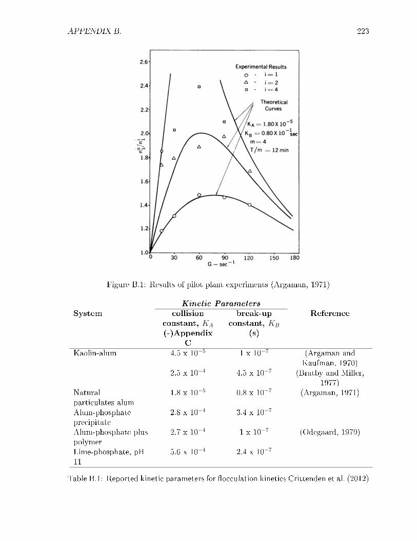
APPENDIX B. 223
Figure B.1: Results of pilot plant experiments (Argaman, 1971)
Kinetic ParametersSystem collision
constant, KA
(-)AppendixC
break-upconstant, KB
(s)
Reference
Kaolin-alum 4.5 x 10⁻⁵ 1 x 10⁻⁷ (Argaman andKaufman, 1970)
2.5 x 10⁻⁴ 4.5 x 10⁻⁷ (Bratby and Miller,1977)
Naturalparticulates-alum
1.8 x 10⁻⁵ 0.8 x 10⁻⁷ (Argaman, 1971)
Alum-phosphateprecipitate
2.8 x 10⁻⁴ 3.4 x 10⁻⁷
Alum-phosphate pluspolymer
2.7 x 10⁻⁴ 1 x 10⁻⁷ (Odegaard, 1979)
Lime-phosphate, pH11
5.6 x 10⁻⁴ 2.4 x 10⁻⁷
Table B.1: Reported kinetic parameters for �occulation kinetics Crittenden et al. (2012)

Appendix C
C.1 Implementation of SST model
C.1.1 Approximation of convective �ux
The Godunov numerical algorithm is a widely used numerical technique in one-dimensional
SST modelling Jeppsson and Diehl 1996; Plosz et al. 2012; Li and Stenstrom 2014.
The numerical method is based on the division of the z-axis by n grid points equally
distributed, such that z = Top and z = Bottom are located half-way between the �rst
two and the last two grid points, respectively, as shown in Figure C.1.
Figure C.1: Locations of grid points in case n=10
Let the index j stand for the space grid point, where the convective �ux F (C, z, t)
in Equation 3.3.1 at the boundary between layers j and j+1 should be replaced by
a numerical convective �ux F numj associated with position zj. Since the model will
eventually be included into a complete water treatment model, simulation speed is a
factor and from the works of Burger et al. (2011), it can be seen that the Godunov
numerical algorithm can be used to approximate kynch batch function, fbk(C(zj,t)):
224

APPENDIX C. 225
Gj = Gj (Cj, Cj+1) =
min
Cj≤C≤Cj+1
fbk if Cj ≤ Cj+1
maxCj≤C≤Cj+1
fbk if Cj > Cj+1
Hence, we obtain the numerical �ux
F numj = F num
j (Cj, Cj+1, t) =
−Qe(zj)Cj+1/A for j = Top− 1, ...., T op−N
Gj −Qe(zj)Cj+1/A for j = Feed− 1, ..., top
Gj −Qe(zj)Cj+1/A+Qu(zj)Cj/A for j = Feed
Gj +Qu(zj)Cj/A for j = Feed+ 1, ...Bottom
+Qu(zj)Cj/A for j = Bottom+ 1, ...Bottom+N
Where N is an arbitrary number of layers above and below the SST boundary to
account for �ow into exiting pipes. The steady state solution has a discontinuity, the
sludge blanket, in the thickening zone so this presented numerical method is stable and
non-oscillatory near discontinuities and it is mass preserving. This implies that even if
a discontinuity is smeared out by numerical di�usion (due to the discretisation), it is
located at the right position, that is, it will have the same speed as the discontinuity of
the analytical solution of 3.3.1.