Mathematical Modelling, Stability Analysis and Control of ... (part-3)/F03432940.pdf · Mathematical Modelling, Stability Analysis and Control of ... strategies such as PID, ... is

IOSR Journal of Engineering (IOSRJEN)

e-ISSN: 2250-3021, p-ISSN: 2278-8719 Vol. 3, Issue 4 (April. 2013), ||V3 || PP 29-40

www.iosrjen.org 29 | P a g e

Mathematical Modelling, Stability Analysis and Control of

Flexible Double Link Robotic Manipulator: A Simulation

Approach

Dinesh Singh Rana Department of Instrumentation, Kurukshetra University, Kurukshetra

Abstract: In present work the various aspects on mathematical modelling, stability and control strategies of flexible double link manipulator have been investigated. A mathematical model of flexible double link

manipulator has been developed using lagrangian method. This mathematical model has been characterized

using classical and modern control theories. Their time domain and frequency domain analysis has been carried

out and our study show that the mathematical model of flexible manipulator is highly unstable. Different control

strategies such as PID, LQR and State feedback controller have been implemented for controlling the tip

position of flexible double link manipulator using MATLAB programming. State feedback controller uses pole

placement approach, while the linear quadratic regulator is obtained by resolving the Riccati equation. The best

control strategy for controlling the tip position of flexible double link manipulator is obtained by

implementation of LQR controller. Finally, this study proven that LQR control method is the best method as

compare to PID and State feedback controller for controlling the flexible link robotic manipulator.

Key words: PID, LQR, MATLAB, State feedback controller

I. INTRODUCTION The dynamics of nonlinear system can be linearized using classical and modern control theory because

it is able to characterize the nonlinear system. The nonlinear differential equations are used to describe the

dynamic characteristics of nonlinear systems [1-4]. Practically, nonlinear systems are solved by numerical and

graphical methods [5-6]. Nonlinear control is the area of control engineering specifically involved with systems

that are nonlinear, time-variant, or both. The response of nonlinear systems to a particular test signals is no

guide to their behaviour to other inputs, since the principal of superposition no longer holds [7]. Robotics is one

of the fields of study of nonlinear system. Robotics is the art, knowledge base, and the know-how of designing,

applying, and using robots in human endeavours. Robotics systems consist of not just robots, but also other [8]

devices and systems that are used together with the robots to perform the necessary tasks. Robotics is an inter-disciplinary subject that benefits from mechanical engineering, electrical and electronics engineering, biology,

and many other disciplines [9]. Robot and robot-like manipulators are now commonly employed in hostile

environment, such as at various places in an atomic plant for handling radioactive materials. Robots are being

employed to construct and repair space stations and satellites. One type of robot commonly used in the industry

is a robotic manipulator or simply manipulator or a robotic arm [8].

Robotic manipulators are mostly used to help in dangerous, monotonous, and tedious jobs. The

growing research interest in flexible link manipulators are due to its several advantages such as low energy

consumption, high speed and high pay load to manipulator weight ratio makes it suitable for aerospace industrial

applications [9-12]. Most of the robotic manipulators are designed and built in a manner to maximize stiffness

in order to minimize the vibration of the end-effectors. To have a high stiffness, additional materials have been

used for the arm. Hence, the heavy rigid manipulators are shown to be inefficient in terms of power consumption or speed with respect to the operating pay load. Many industrial manipulators face the problem of

arm vibrations during high speed motion. In order to improve industrial productivity, it is required to reduce the

weight of the arms and to increase their speed of operation [9-12]. For these purposes, it is desirable to build

flexible robotic manipulators. Due to the importance and usefulness of these robots, a deep investigation for

modelling and control of flexible manipulator is required.

In this paper, a dynamic model of the flexible link which has a rotational and translational motion is

derived by using a Lagrangian method. The prime objective of this paper is to develop the mathematical model

of flexible link manipulators with help of classical and modern control theories and implementation of important

control strategies such as PID, LQR and State feedback controller for controlling the tip position of flexible link

manipulators through MATLAB[13-15]. State feedback controller uses pole placement approach, while the

linear quadratic regulator is obtained by resolving the Riccati equation.

Mathematical Modelling, Stability Analysis And Control Of Flexible Double Link Robotic


II. RESEARCH METHODOLOGY: Mathematical Modeling of Flexible double Link Manipulators

The dynamic model of flexible manipulator involves modeling the rotational base and flexible link

using Lagrange’s method. In order to determine the Lagrangian of system, we need to calculate Potential & Kinetic Energy. The schematic of double link flexible manipulator is illustrated in figure 1.The expression for

potential energy and kinetic energy of double link flexible manipulator is given by equation (1) and (2)

respectively:

Figure 1: Schematic of double link Flexible manipulator

V= P.E. = (1/2).Kstiff.α2 (1)

T = K.E. (total) = K.E.base1 + K.E.Link 1 + K.E.base2 + K.E.Link 2 (2)

= (1/2).Jeq.

.

1

2 + (1/2).JLink.(

.

1 +

.

1) + (1/2).Jeq.

.

2

2 + (1/2).JLink.(

.

2 +

.

2)

Where, θ 1,θ2= Gear Angles of link 1 and link 2 respectively (radians)

α1,α2 = Arm Deflection of link 1 and link 2 respectively (radians)

The assume parameters for double link flexible manipulator are listed in table 1.

Mass of flexible link 1, m = 0.065 kg Length of flexible link 1, L = 0.3 m

Mass of flexible link 2, m = 0.070 kg Length of flexible link 2, L = 0.2 m

End point arc length deflection, d = α*L Armature Resistance, Rm = 2.6 Ω

Equivalent Moment of Inertia at load, Jeq1 = 0.099 kg.m2 Links Moment of Inertia, JArm1 = 0.00195 kg.m2

Equivalent Moment of Inertia at load, Jeq2 = 0.092 kg.m2 Links Moment of Inertia, JArm2 = 0.000933 kg.m2

Equivalent viscous damping coefficient, Beq = 1.99 Gear Box Efficiency, ηg = 0.9

Motor Efficiency, ηm = 0.69 Motor Torque constant, Kt = 0.00767

Back e.m.f. torque constant, Km = 0.00767 Gear Ratio, Kg = 70

Link’s natural frequency, fc = 3.2 Hz Link’s Stiffness, Kstiff = 2Π fc * JArm

Vm=Armature input voltage

Table 1: Parameters of double link flexible manipulator

According to the definition of lagrange function, the lagrangian for double link flexible manipulator is given as:

L = T-V

= (1/2).Jeq1.

.

1

2 +(1/2).JLink.1(

.

1+

.

1)2 -(1/2)kstiff α1

2 +(1/2).Jeq2.

.

2

2+(1/2).JLink.2(.

2+

.

2)2 -(1/2)kstiffα2

2

(3)

We assume that θ & α are two generalized coordinates.

We therefore have two equations:

(δ/ δt).( δL/ δ.

)-( δL/δθ) = To/p + Beq. .

(4)

(δ/ δt).( δL/ δ.

)-( δL/δα) = 0 (5)

Now,

ө

1

α1

α2

ө 2

Link-1

Link-2

Base-1

Base-2



( δL/ δ.

1) = (1/2).(2.Jeq.

.

1) + (1/2). JLink1.2(

.

1) + (1/2). JLink1.2(

.

1)

= Jeq.1

.

+ JLink. .

1+

JLink.

.

1

(δ/ δt).( δL/ δ.

1) = Jeq1.

..

1+ JLink1. 1+ JLink1.

..

1 (6)

Now,

( δL/ δ.

1) = (1/2). JLink1(2.

.

1) + (1/2). JLink1(2.

.

1)

= JLink.1

.

1+ JLink1.

.

1 (7)

( δL/δα1) = -Kstiff (8)

And

( δL/ δ.

2) = (1/2).(2.Jeq.

.

2) + (1/2). JLink2.2(

.

2) + (1/2). JLink2.2(

.

2)

= Jeq.1

.

2 + JLink.

.

2+

JLink.

.

2

(δ/ δt).( δL/ δ.

2) = Jeq2

..

2+ JLink2. 2+ JLink2.

..

2 (9)

Now,

( δL/ δ.

2) = (1/2). JLink2(2.

.

2) + (1/2). JLink2(2.

.

2)

= JLink.2.

2+ JLink2.

.

2 (10)

( δL/δα2) = -Kstiff (11)

Put equations (15), (16), (17), (18), (19) & (20) in equations (13) & (14), we get;

Jeq.1

..

1+ JArm1.( ..

1+ 1) = To/p - Beq.

.

1 (12)

JArm1(

..

1+ 1) + Kstiff.α1 = 0 (13)

Jeq.2

..

2+ JArm2.( ..

2+ 2) = To/p - Beq.

.

2 (14)

JArm2(

..

2+ 2) + Kstiff.α2 = 0 (15)

Where,

To/p = [ηm.ηg.Kt.Kg (Vm-Kg.Km. .

)]/Rm

We will find value of (..

1), (

..

2), ( 1)& ( 2)

Jeq1. ..

1- Kstiff.α1 = [ηm.ηg.Kt.Kg (Vm-Kg.Km.

.

1)]/Rm

Jeq1

..

1 = Kstiff.α1 + [ηm.ηg.Kt.KgVm]/ Rm – [ηm.ηg.Kt.Kg

2.Km. .

1]/Rm- Beq.

.

1

or,

..

1 = [Kstiff.α1]/Jeq1+[ηm.ηg.Kt.KgVm]/Rm.Jeq-[(ηm.ηg.Kt.Kg

2.Km+Beq.Rm). .

1)]/ Rm.Jeq1 (16)

Put value of ..

1 in equation (13);

JArm1. ..

1 + JArm.1 1 + Kstiff.α1 = 0

JArm.1

..

1 + JArm.1 1 = -Kstiff.α1

JArm1.[ Kstiff.α]/Jeq1+[ηm.ηg.Kt.KgVm]/Rm.Jeq1-[(ηm.ηg.Kt.Kg2.Km+Beq.Rm).

.

)]/ Rm.Jeq1 + JArm1 1= -Kstiff.α1

or,

JArm. 1 = -Kstiff.α1 [1 + (JArm1/ Jeq1)] - JArm1[(ηm.ηg.Kt.KgVm)/ Rm.Jeq1] + JArm1(ηm.ηg.Kt.Kg2.Km + Beq.Rm).

.

)/

Rm.Jeq1 )



where,

1 = -Kstiff.α1 {(1/JArm1) + (1/Jeq1) - (ηm.ηg.Kt.KgVm)/Rm.Jeq1 + (ηm.ηg.Kt.Kg2.Km + Beq.Rm).

.

)/Rm.Jeq1

(17)

For second link;

Jeq2. ..

2- Kstiff.α2 = [ηm.ηg.Kt.Kg (Vm-Kg.Km.

.

2)]/Rm

Jeq1

..

2 = Kstiff.α2 + [ηm.ηg.Kt.KgVm]/ Rm – [ηm.ηg.Kt.Kg

2.Km. .

2]/Rm- Beq.

.

2

or,

..

2 = [Kstiff.α2]/Jeq1+[ηm.ηg.Kt.KgVm]/Rm.Jeq2-[(ηm.ηg.Kt.Kg

2.Km+Beq.Rm). .

2)]/ Rm.Jeq2 (18)

Put value of ..

2 in equation (22);

JArm2. ..

2 + JArm.2 2+ Kstiff.α2 = 0

JArm2

..

2 + JArm.2 2 = -Kstiff.α2

JArm2[Kstiff.α2]/Jeq2+[ηm.ηg.Kt.KgVm]/Rm.Jeq2-(ηm.ηg.Kt.Kg2.Km+Beq.Rm)

.

2)/Rm.Jeq2+JArm1 2= -Kstiff.α2

or,

JArm2. 2 = -Kstiff.α2[1+ (JArm2/ Jeq2)] - JArm2[(ηm.ηg.Kt.KgVm)/ Rm.Jeq2] + JArm2(ηm.ηg.Kt.Kg2.Km + Beq.Rm).

.

2)/

Rm.Jeq2 )

And therefore,

2 = -Kstiff.α2{(1/JArm2) + (1/Jeq2) - (ηm.ηg.Kt.KgVm)/Rm.Jeq2 + (ηm.ηg.Kt.Kg2.Km + Beq.Rm).

.

2)/Rm.Jeq2

(19)

The mathematical model may be expressed in state space form. The state space model is expressed as matrix

form, which is essential for the state space control method. For state space representation, the value of

.

1,

.

2,

..

1,

..

2,

.

1 ,

.

2, 1,2 is obtained from equation 16,17,18 and 19.

.

1=0.θ1+0.θ2+0.α1+0.α2+1.

.

1+0

.

2+0.

.

1+0.

.

2 +0.Vm (20)

.

2= 0.θ1+0.θ2+0.α1+0.α2+0..

.

1+1

.

2+0.

.

1+0.

.

2 +0.Vm ( 21)

.

1=

0.θ1+0.θ2+0.α1+0.α2+0..

.

1+0.

.

2+1.

.

1+0.

.

2 + 0.Vm (22)

.

2=

0.θ1+0.θ2+0.α1+0.α2+0..

.

1+0.

.

2+0.

.

1+1.

.

2 + 0.Vm (23)

..

1=0.θ1+0.θ2-kstiff/Jeq1.α1+0.α2+A1..

.

1+0.

.

2+0.

.

1+0.

.

2 +W. Vm (24)

..

2=0.θ1+0.θ2+0.α1-kstiff/Jeq1.α2+0..

.

1+B1.

.

2+0.

.

1+0.

.

2 +X.Vm (25)

1=0.θ1+0.θ2-kstiff(1/Jarm1+1/Jeq1).α1+0.α2+C1..

.

1+0.

.

2+0.

.

1+0.

.

2 +Y. Vm (26)

2= 0.θ1+0.θ2+0. α1-.kstiff(1/Jarm2+1/Jeq2)α2+0.

.

1+D1

.

2+0.

.

1+0.

.

2 +Z. Vm (27)

Where, A1= - (ηm.ηg.Kt. Km Kg

2 + Beq.Rm)/ Rm.Jeq1

B1 = (ηm.ηg.Kt.Kg2.Km + Beq.Rm)/ Rm.Jeq2

C1= (ηm.ηg.Kt. Km Kg2 + Beq.Rm)/ Rm.Jeq1

D1 = (ηm.ηg.Kt.Kg2.Km + Beq.Rm)/ Rm.Jeq2

Matrix form can be obtained from equations 20,21,22,23,24,25,26 & 27.



(28)

(29)

C = [1 1 1 1 0 0 0 0] D = [0]

Substituting the values of parameters of double link flexible manipulators in above equation 28 and 29, we

obtain the following model:



(30)

III. RESULTS AND DISCUSSION: Stability analysis and controller implementation of Flexible Link

Manipulator

The Transfer function for double link flexible manipulator has been derived from its state space model i.e. using

equation 38 and 39. θ(s) /Vm=G(s)= -45.25s7+120.5s6+6.984s5+1131s4+2472s3+63.11s2-60.7s+28.1

s8-.5475s7+815.2s6-418.7s5+22.2s4-86.6s3-132.6s2

By using the root- Locus method, it is possible to determine the value of the loop gain K that will make

the damping ratio of the dominant closed-loop poles as prescribed. If the location of an open-loop pole or zero is

a system variable, then the root-locus method suggests the way to choose the location of an open- loop pole or

zero. The root locus plot of above transfer function is shown in figure 2.

Figure 2: Root Locus Plot for double link Flexible manipulator



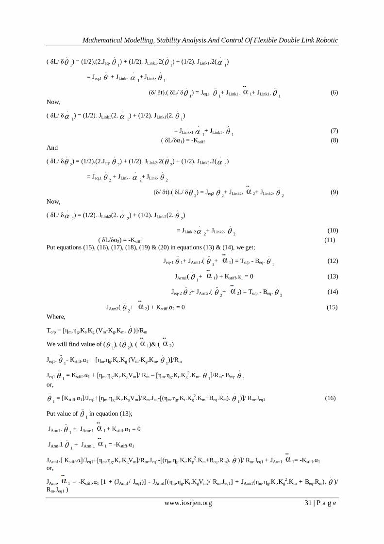
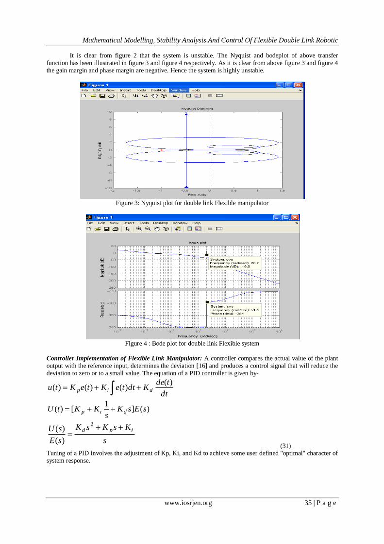
It is clear from figure 2 that the system is unstable. The Nyquist and bodeplot of above transfer

function has been illustrated in figure 3 and figure 4 respectively. As it is clear from above figure 3 and figure 4

the gain margin and phase margin are negative. Hence the system is highly unstable.

Figure 3: Nyquist plot for double link Flexible manipulator

Figure 4 : Bode plot for double link Flexible system

Controller Implementation of Flexible Link Manipulator: A controller compares the actual value of the plant

output with the reference input, determines the deviation [16] and produces a control signal that will reduce the

deviation to zero or to a small value. The equation of a PID controller is given by-

dt

tdeKdtteKteKtu dip

)()()()(

)(]1

[)( sEsKs

KKtU dip

s

KsKsK

sE

sU ipd

2

)(

)(

(31)

Tuning of a PID involves the adjustment of Kp, Ki, and Kd to achieve some user defined "optimal" character of

system response.



Figure 5: PID Controller of Flexible link system

Where, Kp = Proportional Gain ; Kd = Derivative Gain; Ki = Integral Gain; R(s) = reference signal

G(s) = Transfer Function of flexible link manipulator; e(s) = error signal; u(s) = plant input

y(s) = output from the plant

Therefore, the open-loop transfer function of the diagram can be found as shown by the equation:

Y(s)/U(s) = G(s) * [KP + Kds + (Ki/s)] (32)

Where G(s) is the plant transfer function.

The open-loop transfer function in equation (32) can be implemented into Matlab by using the m-file code. The

transfer function from the Laplace transforms or from the state space representation can be used. This transfer

function assumes that both derivative and integral control will be needed along with proportional control. This

open-loop transfer function can be modeled in Matlab. The function polyadd is not originally in the Matlab

toolbox. It has to be copied to a new m-file to use it. This transfer function is assumed that both derivative and

integral control will be needed along with proportional control. The actual control of this system could be stated by subjecting step input and its response which has been shown in figure 6.

Figure 6: Closed loop PID Response of double link flexible manipulator

State Feedback Controller

The pole placement approach specifies all closed-loop poles in comparison to conventional design

approach which specifies only dominant closed loop poles [8]. In pole-placement approach the desired closed-

loop poles can be arbitrarily placed, provided the plant is completely state controllable. In designing a system

using the pole placement approach several different sets of desired closed-loop poles need to be considered, the

response characteristics compared, and the best one chosen.

Consider a control system x = Ax+Bu

y = Cx+ Du (33)

Where, x = state vector (n-vector); y = output signal (scalar)

u = control signal (scalar); A= n × n constant matrix

B = n × 1 constant matrix; C= 1 × n constant matrix

D = constant (scalar)

Let choose the control signal to be.

u = -Kx (34)



This means that the control signal u is determined by an instantaneous state. Such a scheme is called

state feedback. The = 1 × n matrix K is called the state feedback gain matrix. A block diagram for this system is

shown in figure 7.

Figure 7: Design of control system in state space

Substituting Equation (34) into equation (33) gives

x(t) = (A-BK) x (t)

The solutions of this equation is given by

x(t) = e(A-BK)t

x (0) (35)

Where x(0) is the initial state caused by external disturbances. The stability and transient response

characteristics are determined by the Eigen values of matrix A-BK. If matrix K is chosen properly, the matrix

A-BK can be made an asymptotically stable matrix, and for x (0)≠0 , it is possible to make x (t) approach 0 as t

approaches infinity. The eigen-values of matrix A-BK are called the regular poles. If these regulator poles are placed in the left-half s plane, then x (t) approaches 0 as t approaches infinity. The problem of placing the

regular poles (closed-Loop poles) at the desired location is called a pole- place-placement problem.

Pole-placement problems can be solved easily with MATLAB. MATLAB has two commands- acker and place

– for the computation of feedback gain matrix K. The command acker is based on Ackerman’s formula. This

command applies to single-input system only. [17]. The most commonly used commands are

K= acker(A,B,J)

or, K= place(A,B,J)

where A and B are system matrices and J is a row vector containing the desired closed-loop poles. These

commands returns the gain vector K.

CASE 1

Choose the desired closed -loop poles at

-2+j*4, -2-j*4, -3+2*j, -3-2*j, -6, -2, -10, -4 A unit step response of flexible double link system using feedback gain matrix (Ko) from pole-placement

method is shown in figure 8.

Figure 8: Unit step response of double link of flexible manipulator using Ackerman method for case1

CASE 2

Choose the desired closed -loop poles at

-3+2j, -3-2j, -4+2j, -4-2j, -3, -2, -1, -4



A unit step response of flexible double link system using feedback gain matrix (Ko) from pole-placement

method is shown in figure 9.

Figure 9: Unit step response of double link of flexible manipulator using Ackerman method for case2

Linear Quadratic Regulator

The theory of optimal control is concerned with operating a dynamic system at minimum cost. The

case where the system dynamics are described by a set of linear differential equations and the cost is described

by a quadratic functional is called the LQ problem. One of the main results in the theory is that the solution is

provided by the linear-quadratic regulator (LQR). The "cost" (function) is often defined as a sum of the

deviations of key measurements from their desired values. In effect this algorithm therefore finds those

controller settings that minimize the undesired deviations, like deviations from desired altitude or process

temperature [17]. Often the magnitude of the control action itself is included in this sum as to keep the energy

expended by the control action itself limited. The LQR algorithm is, at its core, just an automated way of finding

an appropriate state feedback controller. Consider the optimal regulator given by system equation:

(36)

That determines the matrix K of optimal control vector

u(t) = -Kx(t) (37)

So as to minimize the performance index

0

** )( dtRuuQxxJ (38)

Where, Q and R is a positive definite or real symmetric matrix. The block diagram showing the optimal configuration is shown in figure 10.

Figure 13 Quadratic Optimal Regulator System

Substituting equation (37) into (36), we obtain

x = Ax –BKx = (A-BK)x Substituting equation (37) into (38), we obtain

Let us set

x*(Q + K*RK)x = -d/dt (x*Px)

Where, P is positive definite Hermition-Matrix.

x*(Q + K*RK)x = -x*[(A-BK)*P + P (A-BK)]x

Comparing both sides of this equation and notice that this equation must hold true for any x, we require that

(A-BK)*P + P(A-BK) = -(Q + K*RK) (39)



It can be proved that if A-BK is a stable matrix, there exist a [8] positive definite matrix that satisfies equation

(39).

The performance index J can be evaluated as

= -x*(∞)Px(∞)+ x*(0)Px(0) (40)

Since all Eigen values of A-BK are assumed to have negative real parts, we have x(∞)---0.

Therefore, we obtain J= x*(0)Px(0)

Thus, the performance index J can be obtained in terms of initial condition x(0) and P.

To obtain the solution of quadratic optimal control problem, we proceed as follows

R = T*T Where, T is a non-singular matrix. Then equation (39) can be written as (A*-K*B*) P + P(A-BK) + Q

+ K*T*TK =0.

The minimization of J w.r.t. K requires the minimization of

x*[TK-(T*)-1 B*P]*[TK-(T*)-1B*P]x w.r.t. K

The minimum occurs when it is zero or when

TK = (T*)-1B*P

Hence, K = T-1(T*)-1B*P = R-1B*P (41) Equation (41) gives the optimal matrix K. Thus, the optimal control law to the quadratic optimal control

problem, when the performance index is given by equation (38) is linear and is given by

u(t) = -Kx(t) = R-1

B*Px(t). The matrix P in equation (41) must satisfy equation (39) or the following

reduced equation:

A*P +PA-PB R-1B*P + Q = 0 (42)

Equation (42) is called the reduced – matrix Riccati equation. The design steps may be stated as follows:

i. Solve equation (42), the reduced – matrix Riccati equation, for matrix P.

ii.Substitute this matrix P into equation (41). The resulting matrix K is the optimal matrix.

The Unit step response of double link flexible manipulator using LQR method is illustrated in figure14.

Figure 14 : Unit step response of double link flexible manipulator using LQR method

Where, x1 corresponds to θ1 x2 corresponds to θ2 x3 corresponds to α1

x4 corresponds to α2 x5 corresponds to .

1 x6 corresponds to

.

2

x7 corresponds to .

1 x8 corresponds to

.

2



IV. CONCLUSIONS The various aspects on mathematical modelling, stability and control strategies of flexible double link

robotic manipulator have been investigated in this paper. A mathematical model of flexible double link

manipulator has been developed using lagrangian method. Mathematical model of flexible double link robotic

manipulator have been characterized using classical and modern control theories and its time domain and

frequency domain analysis has been carried out. Our study shows that the mathematical model of flexible

manipulator is highly unstable system. Different control strategies such as PID, LQR and State feedback

controller have been implemented for controlling the tip position of flexible double link manipulator. State

feedback controller uses pole placement approach, while the linear quadratic regulator is obtained by resolving

the Riccati equation.

It was concluded from our results of implementation of various controllers for flexible double link manipulator

problem that the state feedback and linear quadratic regulator (LQR) controllers providing the better performance than conventional PID controllers. The performance of state feedback controller is depending upon

pole positions and hence it becomes hit and trial procedure for controlling the flexible double link manipulator.

The best control strategy for controlling the tip position of flexible double link manipulators is obtained by

implementation of LQR controller. Finally it can be conclude from our study that LQR control method is the

best method among PID and State feedback controller to control the flexible double link manipulator.

REFERENCES [1]. Dinesh Singh Rana and Rajiv Sharma, Fuzzy Logic Based Automation of Green House Environmental

parameters for Agro-industries-A Simulation Approach, International Journal of Applied Engineering

Research, 6 (5) 2011, 662-666

[2]. Rajvir Sharma, Dinesh Singh Rana etal, A Fuzzy Logic based Automatic Control of Rotary Crane (A

Simulation Approach), Advance Materials Research, Vols.,403-408, 2012, 4659-4666

[3]. Dinesh Singh Rana, Fuzzy logic based automation and control simulation of Sulfuric acid manufacturing

process: A case study, IOSR Journal of Engineering (IOSRJEN) 2(8) 2012, 19-35

[4]. Dinesh Singh Rana, FLC and PLC based Process Optimization and Control of Batch Digester in Pulp nd

Paper Mill, Res. J. Engineering Sci., Vol. 1(2), August (2012) 51-62

[5]. Dinesh Singh Rana, Fuzzy logic based control of Superheater and Boiler unit and Amine treating unit for

the automation of CO2 filtration process: A Simulation Approach, International Journal of Applied Engineering Research 7(11)2012, 1231–1252

[6]. Dinesh Singh Rana, Fuzzy logic based automatic control of compressor and regenerator units used in the

CO2 filtration process: A Simulation Approach, International Journal of Applied Engineering Research

7(11)2012, 1263–1278

[7]. I. J Nagrath and M.Gopal, Control systems engineering (third edition. New Age international (P) Ltd.

Pub., 2003)

[8]. R.K mittal, I.J Nagrath, Robotics and control (Tata McGraw Hill) Saeed B.Niku, Introduction to

Robotics-Analysis,Systems and Applications

[9]. S.K. Dwivedy and P. Eberhard, Dynamic analysis of flexible manipulators, Mechanism and Machine

theory, 41(7) 2006, 749-777

[10]. H. yang, H. Krishnan etal,, Variable structure controller design for flexible-link Robits under gravity, Proc. 37th IEEE Conf. on Decision and Control, Tampa, Florida USA dec.1998, 1494-1498.

[11]. CHEN Wei, YU Yueqing etal, Vibration controllability of underactuated Robots with flexible links, Proc.

International Technology and innovation Conf. 2007, , 1872-1877.

[12]. Bansal, Goel and Sharma “MATLAB & its application in Engineering (Pearson Edition)

[13]. Stephen j. Chapman, MATLAB Programming for Engineers (Thomson Learning Inc., 2004)

[14]. Andrew Knight; Basics of MATLAB and Beyond (Chapman and Hall/crc.) Katsuhiko Ogata, Modern

Control Engineering ( PHI Eastern Economy Edition1996)

[15]. Arvind kumar; Modeling and Implementation of control strategies for Inverted Pendulum system, A

M.Tech, Dissertation under the supervision of Dr. Dinesh Singh Rana , Kurukshetra University,

Kurukshetra.

Documents

Mathematical Modelling, Stability Analysis and Control of ... (part-3)/F03432940.pdf · Mathematical Modelling, Stability Analysis and Control of ... strategies such as PID, ... is