Mathematical Models, Algorithms, and Statistics of ...people.math.sc.edu/czabarka/Theses/thesis_orlova.pdfMathematical Models, Algorithms, and Statistics of Sequence ... Alignment

Mathematical Models, Algorithms, and Statistics of Sequence

Alignment

By

Tatiana Aleksandrovna Orlova

SpecialistSaratov State University 2002

Submitted in Partial Fulfillment of the Requirements

for the Degree of Master of Science in

Mathematics

College of Arts and Sciences

University of South Carolina

2010

Accepted by:

Eva Czabarka, Director of Thesis

Joshua Cooper, Second Reader

James Buggy, Interim Dean of the Graduate School

Acknowledgments

I would like to thank Dr. Eva Czabarka and Dr. Joshua Cooper for their helpful

advice and patience.

ii

Abstract

The problem of biological sequence comparison arises naturally in an attempt to

explain many biological phenomena. Due to the combinatorial structure and pat-

tern preserving properties of the sequences it has attracted not only biologists, but

also mathematicians, statisticians and computer scientists. In this work we study

one of the most effective tools widely used for comparison of biological sequences -

sequence alignment. We present the basic theory of sequence alignment from com-

putational, biological, and statistical perspectives. We will also present and analyze

results of computer simulations that effectively illustrate one possible application of

this theory.

iii

Contents

Acknowledgments . . . . . . . . . . . . . . . . . . . . . . . . . . . . . . . ii

Abstract . . . . . . . . . . . . . . . . . . . . . . . . . . . . . . . . . . . . . iii

List of Tables . . . . . . . . . . . . . . . . . . . . . . . . . . . . . . . . . . v

List of Figures . . . . . . . . . . . . . . . . . . . . . . . . . . . . . . . . . vi

Chapter 1. Introduction: Where Mathematics Meets Biology . . 1

1.1. The Organized Complexity of Life . . . . . . . . . . . . . . . . . . . 1

1.2. Biological Sequences and Their Patterns . . . . . . . . . . . . . . . . 4

1.3. Biological Sequence Comparison . . . . . . . . . . . . . . . . . . . . 9

Chapter 2. Sequence Alignment . . . . . . . . . . . . . . . . . . . . . . 11

2.1. Pairwise Sequence Alignment . . . . . . . . . . . . . . . . . . . . . . 11

2.2. Scoring Schemes . . . . . . . . . . . . . . . . . . . . . . . . . . . . . 14

2.3. Alignment Algorithms . . . . . . . . . . . . . . . . . . . . . . . . . . 27

Chapter 3. Statistics of Local Sequence Alignment . . . . . . . . 50

3.1. Hypothesis Testing . . . . . . . . . . . . . . . . . . . . . . . . . . . . 50

3.2. Random Variables and Random Processes . . . . . . . . . . . . . . . 53

3.3. Ungapped Local Alignment Scores Statistics . . . . . . . . . . . . . . 62

3.4. Gapped Local Alignment Scores Statistics . . . . . . . . . . . . . . . 78

Chapter 4. Conclusions . . . . . . . . . . . . . . . . . . . . . . . . . . . 87

Bibliography . . . . . . . . . . . . . . . . . . . . . . . . . . . . . . . . . . . 89

Appendix A. C++ Code . . . . . . . . . . . . . . . . . . . . . . . . . . . 94

iv

List of Tables

Table 1.1 Amino acids and their abbreviations. . . . . . . . . . . . . . . 7

Table 3.1 Robinson & Robinson amino acid counts. . . . . . . . . . . . . 80

Table 3.2 Simulations results. . . . . . . . . . . . . . . . . . . . . . . . . 80

Table 3.3 Known estimates for λ and µ. . . . . . . . . . . . . . . . . . . 81

v

List of Figures

Figure 1.1 Central dogma of molecular biology . . . . . . . . . . . . . . . 4

Figure 1.2 DNA chemical structure . . . . . . . . . . . . . . . . . . . . . 5

Figure 1.3 DNA complementarity . . . . . . . . . . . . . . . . . . . . . . 5

Figure 1.4 Lambda repressor protein bound to a lambda operator DNA

sequence. . . . . . . . . . . . . . . . . . . . . . . . . . . . . . 8

Figure 2.1 BLOSUM62 substitution matrix . . . . . . . . . . . . . . . . . 22

Figure 2.2 Alignment graph for sequences ATACTGG and GTCCGTG. . 28

Figure 2.3 Another alignment graph for ATACTGG and GTCCGTG. . . 29

Figure 2.4 Extended alignment graph. . . . . . . . . . . . . . . . . . . . 33

Figure 2.5 Extended alignment network . . . . . . . . . . . . . . . . . . . 45

Figure 2.6 The optimal global path. . . . . . . . . . . . . . . . . . . . . . 46

Figure 2.7 Global alignment score matrix (S(i, j)) . . . . . . . . . . . . . 47

Figure 2.8 The optimal local path. . . . . . . . . . . . . . . . . . . . . . 48

Figure 2.9 Local alignment score matrix (S(i, j)) . . . . . . . . . . . . . 49

Figure 3.1 Ungapped alignment and its accumulative score. . . . . . . . . 63

Figure 3.2 Random walk corresponding to the ungapped local alignment. 66

Figure 3.3 Counts of large alignment scores, L = 400 . . . . . . . . . . . 82

Figure 3.4 Probability density plot of simulated and estimated data for

sequences of length L=40. . . . . . . . . . . . . . . . . . . . . 83

vi

Figure 3.5 Cumulative probability distribution plot of simulated and estimated

data for sequences of length L = 40. . . . . . . . . . . . . . . 83


sequences of length L = 100. . . . . . . . . . . . . . . . . . . . 84











vii

Chapter 1

Introduction: Where Mathematics Meets

Biology

“Biology is mathematics’ next physics, only better”. Joel Cohen [12]

1.1. The Organized Complexity of Life

In 1953 Francis Crick, Rosalind Franklin, James Watson, and Maurice Wilkins

determined the structure of DNA. This important event became a start of theoret-

ical study of biological sequences. In his book “Life Itself. Its Origin and Nature”

[14] Crick gave a very intuitive explanation of the general nature of life from an

information-theoretical perspective, which can serve as a perfect start in establishing

a connection between biology and mathematics.

He starts with the idea that, the high degree of organized complexity of life

implies the need to store and process large amount of information. Thus, Nature has

to provide an effective mechanism for this important task. Such a mechanism must

1

perform two functions: information storage and replication. Information storage

must be stable, which means that the information must be stored over a sufficiently

long period of time, and replication must be accurate, which means that the copying

can make only a small number of errors called mutations. Lack of accuracy can lead

to accumulated errors and decay, but perfect accuracy is not required. Moreover, we

must have a small number of mutations and require that they must be copied faithfully

through generations. Most mutations lead to maladaptive changes but some might

lead to improvement. There is no mechanism to produce only favorable mutations,

which leaves chance to be the only source of true novelty. It is always possible for

any rare chance event to become very common once this change is favored by the

environment. This gives the living system its primary mechanism to improve itself.

Note that neither replication nor mutation alone can explain both similarity and

diversity of life, as we can see it everywhere around. Thus, the presence of both

mechanisms is required [14].

Effectively dealing with large amounts of information in this manner puts some

requirements on the mechanism. Recall that it needs to provide the system with easy

storage, easy replication, easy error correction, and stability of information. The key

idea is that an efficient way to do this requires the use of the combinatorial principle.

That is, we express the information by using only a small number of types of standard

units, but we combine them in many different ways. Similar to how we use words

to form sentences in human language, life uses linear strings of standard units. It is

required that in any language suitable for communication the number of words must

be relatively small compared to the number of sentences they can produce. Nature

follows the same principle requiring a small number of basic units, but the number

of structures these units can form must be very large. Moreover, in order to carry

information these structures must not be completely regular. The natural question

is what Nature chose for these basic units and why.

2

Carbon is one the most abundant elements in the universe. It has a perfect

balance between valence electrons available and valence electrons needed to fill the

outer shell. This allows carbon to excel in bonding with itself and other atoms,

and to form long chains, so it can build arbitrarily long and complex structures.

Moreover, energy required to make and break carbon bonds is at the appropriate

level for building molecules which are stable and reactive [46]. Note, that there are

other elements that possess some of these properties but only carbon has all of them

[47]. Taking all the above into account Nature’s choice of carbon compounds as

units is obvious. Crick concludes that information transmission with the required

properties is naturally achieved through chemical reactions between combinatorial

structures made of carbon compounds [14].

We will only consider one-dimensional linear structures, known as biopolymers,

or biological sequences.

3

1.2. Biological Sequences and Their Patterns

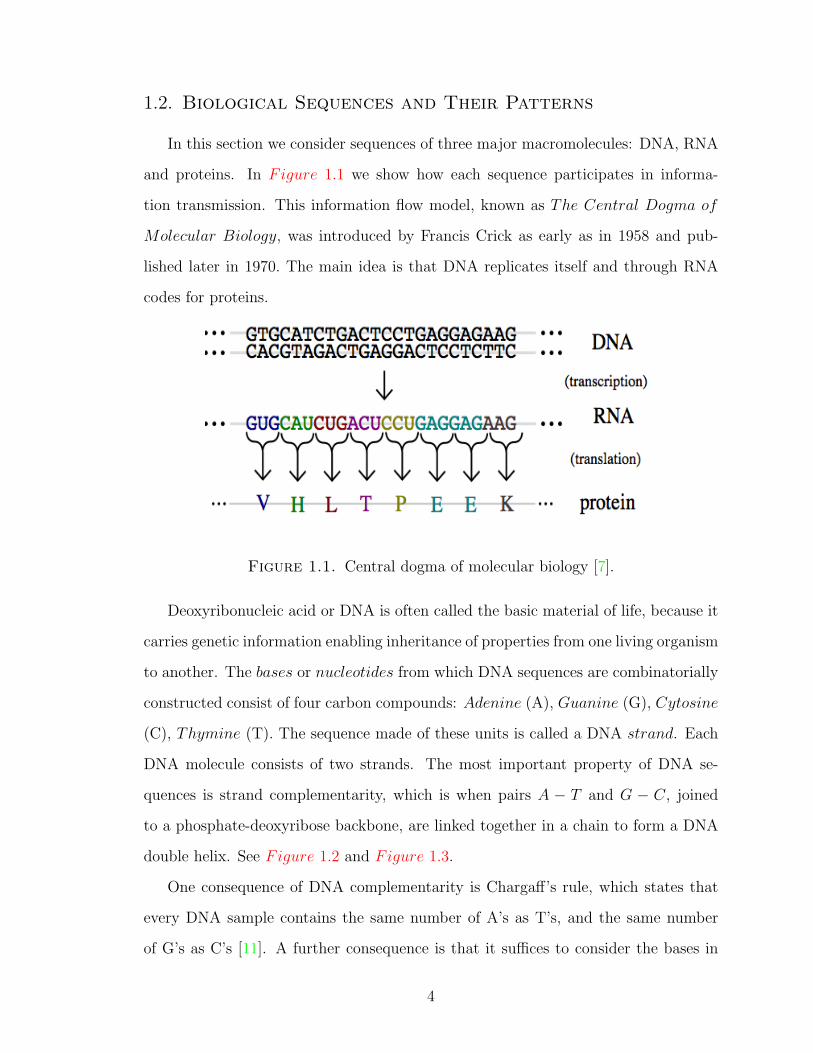
In this section we consider sequences of three major macromolecules: DNA, RNA

and proteins. In Figure 1.1 we show how each sequence participates in informa-

tion transmission. This information flow model, known as The Central Dogma of

Molecular Biology, was introduced by Francis Crick as early as in 1958 and pub-

lished later in 1970. The main idea is that DNA replicates itself and through RNA

codes for proteins.

Figure 1.1. Central dogma of molecular biology [7].

Deoxyribonucleic acid or DNA is often called the basic material of life, because it

carries genetic information enabling inheritance of properties from one living organism

to another. The bases or nucleotides from which DNA sequences are combinatorially

constructed consist of four carbon compounds: Adenine (A), Guanine (G), Cytosine

(C), Thymine (T). The sequence made of these units is called a DNA strand. Each

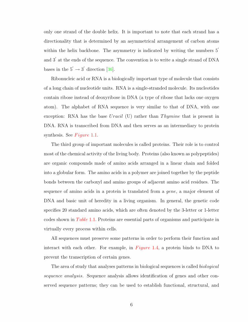
DNA molecule consists of two strands. The most important property of DNA se-

quences is strand complementarity, which is when pairs A − T and G − C, joined

to a phosphate-deoxyribose backbone, are linked together in a chain to form a DNA

double helix. See Figure 1.2 and Figure 1.3.

One consequence of DNA complementarity is Chargaff’s rule, which states that

every DNA sample contains the same number of A’s as T’s, and the same number

of G’s as C’s [11]. A further consequence is that it suffices to consider the bases in

4

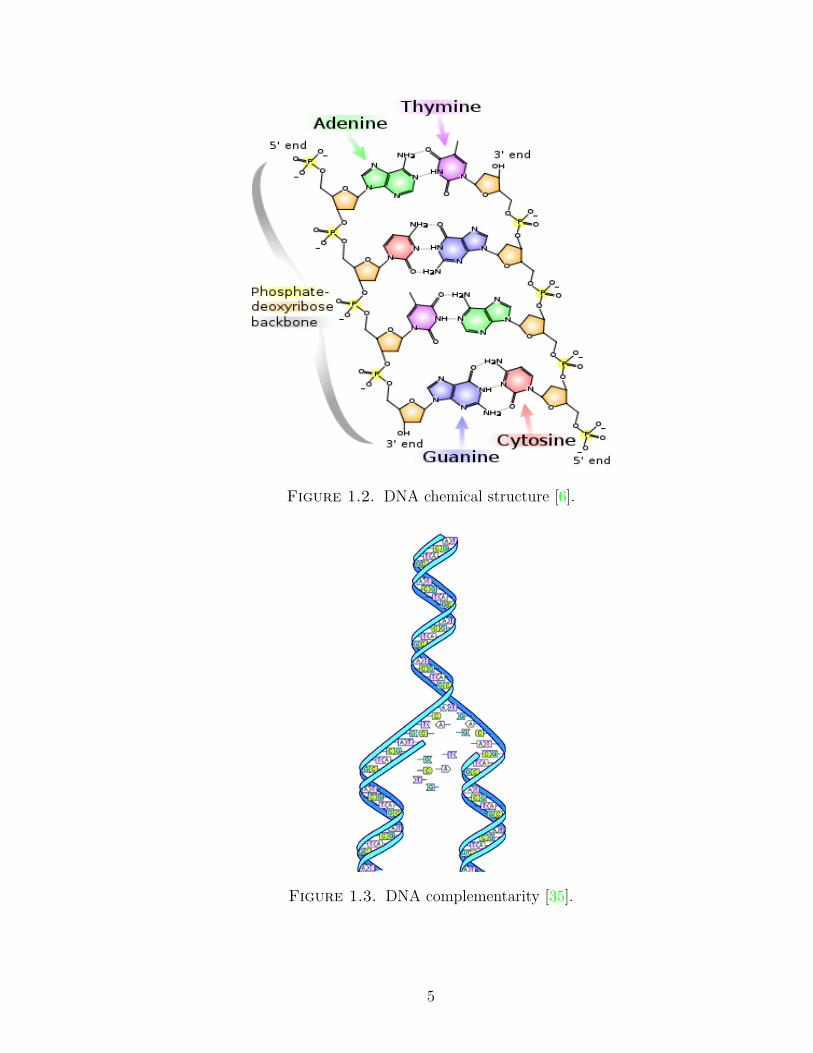
Figure 1.2. DNA chemical structure [6].

Figure 1.3. DNA complementarity [35].

5

only one strand of the double helix. It is important to note that each strand has a

directionality that is determined by an asymmetrical arrangement of carbon atoms

within the helix backbone. The asymmetry is indicated by writing the numbers 5′

and 3′

at the ends of the sequence. The convention is to write a single strand of DNA

bases in the 5′ → 3

′direction [36].

Ribonucleic acid or RNA is a biologically important type of molecule that consists

of a long chain of nucleotide units. RNA is a single-stranded molecule. Its nucleotides

contain ribose instead of deoxyribose in DNA (a type of ribose that lacks one oxygen

atom). The alphabet of RNA sequence is very similar to that of DNA, with one

exception: RNA has the base Uracil (U) rather than Thymine that is present in

DNA. RNA is transcribed from DNA and then serves as an intermediary to protein

synthesis. See Figure 1.1.

The third group of important molecules is called proteins. Their role is to control

most of the chemical activity of the living body. Proteins (also known as polypeptides)

are organic compounds made of amino acids arranged in a linear chain and folded

into a globular form. The amino acids in a polymer are joined together by the peptide

bonds between the carboxyl and amino groups of adjacent amino acid residues. The

sequence of amino acids in a protein is translated from a gene, a major element of

DNA and basic unit of heredity in a living organism. In general, the genetic code

specifies 20 standard amino acids, which are often denoted by the 3-letter or 1-letter

codes shown in Table 1.1. Proteins are essential parts of organisms and participate in

virtually every process within cells.

All sequences must preserve some patterns in order to perform their function and

interact with each other. For example, in Figure 1.4, a protein binds to DNA to

prevent the transcription of certain genes.

The area of study that analyses patterns in biological sequences is called biological

sequence analysis. Sequence analysis allows identification of genes and other con-

served sequence patterns; they can be used to establish functional, structural, and

6

Amino Acid 3-Letter 1-Letter

Alanine Ala AArginine Arg R

Asparagine Asn NAspartic acid Asp D

Cycteine Cys CGlutamic acid Glu E

Glutamine Gln QGlycine Gly G

Histidine His HIsoleucine Ile ILeucine Leu LLysine Lys K

Methionine Met MPhenylalanine Phe F

Proline Pro PSerine Ser S

Threonine Thr TTryptophan Trp W

Tyrosine Tyr YValine Val V

Table 1.1. Amino acids and their abbreviations.

evolutionary relationship among proteins; and they provide a reliable method for in-

ferring the biological functions of newly sequenced genes [10]. The basic idea is to

be able to read any biological sentence, see and understand the genes and conserved

patterns it encodes, as one would read a text in a familiar language.

For example, when a new protein is found, scientists usually have little idea about

its function. Direct experimentation on a protein of interest is often costly and time-

consuming [39]. As a result, one common approach to inferring the protein’s function

is to find similar proteins that have been studied and are stored in database. The

functions of these proteins may give us a clue of the unknown function of our protein.

If necessary, the information thus inferred can be verified experimentally.

One remarkable finding made through sequence comparison concerns the origins

of cancer. In 1983, a paper by Doolittle, et al. [17] appearing in Science reported a

28-amino-acid sequence for platelet derived growth factors, a normal protein whose

7

Figure 1.4. Lambda repressor protein bound to a lambda operatorDNA sequence [45], [8].

function is to stimulate cell growth. By searching against a small protein database

created by himself, Doolittle found that the sequence is almost identical to a sequence

of ν-sis, an oncogene causing cancer in woolly monkeys. This finding changed the

way oncogenesis is seen and understood. Today, it is generally accepted that cancer

is caused by a normal growth gene which is switched on at the wrong time [10].

8

1.3. Biological Sequence Comparison

From now on we only look at pairs of biological sequences, where both sequences

must represent either two DNA or two protein sequences. The major question we ask

is how similar or homologous these pairs of sequences are.

Definition 1. We call two biological sequences homologous if they are evolutionarily

similar, i.e., were derived from a common ancestor.

We want to be able to compare these sequences to see whether they are homologous

or not. Then, the next step would be to find a method of comparison that measures

the extent of this homology. The method that has been effectively used for both tasks

is called sequence alignment.

The pairwise sequence alignment method compares a pair of sequences and assigns

to it a value called a score. Three important aspects are involved in this process:

computational, biological, and statistical.

From the computational perspective we can look at the alignment problem as the

problem of comparing two text strings in a given alphabet. This problem has been

extensively studied in the field of computer science. A purely computational solution

to this problem will score a pair of text strings given an algorithm and a scoring rule.

As a result, every pair of strings receives a score.

In the case of biological sequence comparison we want a biologically relevant

alignment. By this we mean that we would like the resulting alignment to be probable,

i.e., to have some chance of one sequence deriving from the other according to the

explanation suggested by the alignment. This can be achieved by the special design

of scoring rules, based on some essential molecular evolution assumptions combined

with probabilistic techniques.

Finally, we need to understand what the fact that two sequences received a par-

ticular score can tell us about their homology. The field of mathematical statistics

provides powerful tools to answer this question.

9

So far we showed some biological examples where the question of sequence compar-

ison arises naturally and the answer to this question helps to explain some biological

phenomena. The further presentation of material will go as follows: Chapter 2 takes

a more detailed look at the sequence alignment problem from computational and

biological perspectives. Chapter 3 is devoted to statistical methods that have been

developed to assess the significance of alignment scores. At the end of Chapter 3 we

also present and analyze the results of computer simulation that effectively illustrate

the use of the computational, biological and statistical theory discussed in this work.

We conclude by summarizing main results in Chapter 4.

10

Chapter 2

Sequence Alignment

“Share our similarities, celebrate our differences.” M. Scott Peck

2.1. Pairwise Sequence Alignment

A standard method for biological sequence comparison is sequence alignment.

Sequence alignment is essentially nothing else but matching certain parts of two (or

more) sequences. This, of course, can be done in many different way, so one must

judge the goodness of such an alignment in some ways — preferably through a suitably

defined model that is motivated by how evolution works on the molecular level. One

then needs to find the best alignment according to our measure of goodness. To see

how it is usually done in practice, we need to start with some basic definitions.

11

Definition 2. Let Σ = σ1, . . . , σ` be an alphabet, and let X = x1x2 . . . xm and

Y = y1, y2, . . . yn be two sequences over Σ. We extend our alphabet Σ by adding a

special symbol “−”, which denotes space. An alignment of sequences X and Y is a

two-row matrix A with entries in Σ ∪ − such that

1. The first (second) row contains the letters of X (Y ) in order;

2. One or more spaces “−” may appear between two consecutive letters of Σ in

each row;

3. Each column contains at least one letter of Σ [10].

From a biological point of view, an alignment of two sequences poses a hypoth-

esis about how the sequences evolved from their most recent common ancestor. An

alignment accounts for the following three mutational events:

• Substitution (also called point mutation) - A nucleotide (amino acid) is re-

placed by another.

• Insertion - One or several nucleotides (amino acids) are inserted at a position

in a sequence.

• Deletion - One of several nucleotides (amino acids) are deleted from a se-

quence [10].

Definition 3. For 1 6 i, j 6 ` and xi, yj ∈ Σ a column(xiyj

)of an alignment A is

called a match if xi = yj and mismatch (or substitution) if xi 6= yj. A column(−yj

)is

called an insertion and a column(xi−

)is called a deletion. Columns

(−yj

)and

(xi−

)are

also called indels. The column(−−

)is not allowed in an alignment. Also, it is common

to refer to columns of the alignment as sites.

Definition 4. A gap in an alignment is defined as a sequence of spaces “− ” located

between two letters in a row. We will use p to denote a gap length. We say an

alignment is gapped or ungapped to emphasize whether indels are allowed or not in

the alignment.

12

For example, in the alignment

A =

A − T A C − T G G

− G T C C G T − G

the two sequences are identical in the third, fifth, seventh, and ninth columns - they

are the matches. There is a mismatch in the fourth column, first and eighth columns

are deletions, and second and sixth columns are insertions.

We need a rule to tell us the “goodness” of each possible alignment. Traditionally,

a scoring matrix is used for this purpose.

Definition 5. Consider an alphabet Σ = σ1, . . . , σ` and a function s : Σ× Σ→ Z

that assigns a score s(σi, σj) to each pair of letters (σi, σj). Then for 1 6 i, j 6 ` a

matrix (s(σi, σj)) is called a scoring matrix for an alphabet Σ.

In the case of gapped alignment, having a scoring matrix is not enough. We also

need a way to score gaps.

Definition 6. A gap penalty function is a function ∆ : k → Z− ∪ 0 that assigns a

non-positive integer penalty ∆(k) for every gap of length 1 6 k 6 max(n,m) in an

alignment.

Definition 7. A scoring matrix and a gap penalty function are called a scoring

scheme.

Definition 8. An alignment score is the sum of scores of each pair of symbols in the

alignment. This important property is called additivity.

13

2.2. Scoring Schemes

2.2.1. Biological Perspective. The major biological question we want to an-

swer is whether the two sequences are homologous; thus, we would like to have such

a scoring scheme that answers this question as correctly as possible. When sequence

comparison was first introduced, the scoring schemes were extremely simple. For ex-

ample, for each match the score of “1” was used and for each mismatch and insertion

or deletion a value of “ − 1” were assigned. This rule was too simple to produce

a biologically meaningful result. Then, biologists who became experienced enough

with sequence data started using their knowledge to design more sophisticated scor-

ing rules. All of these rules were somewhat unsubstantiated and usually worked just

for a very small number of problems.

It is intuitively obvious that taking random sequences that were generated accord-

ing to a given underlying letter-distribution, and aligning these sequences randomly,

the frequency of letter pairs should differ depending on the distribution of the letters.

Even in these chance alignments, pairs of frequent letters appear more often than

pairs of unfrequent letters. In real alignments, which have biological meaning, one

would expect identities and conservative substitutions to be more frequent than they

would appear in chance alignments, thus, these columns should contribute positive

terms to the score of an alignment. Similarly, non-conservative changes should be less

frequent in real alignments than they would be in chance alignments, therefore the

columns corresponding to non-conservative changes should contribute negative terms

to the alignment score. In the absence of a rigorous theory, experience helped scien-

tists to decide whether an aligning pair is conservative or not and up to what degree,

thus allowing them to come up with scores that “work” based on intuition. Later,

developments in computer technology and the increase in sequence data resources

led to much more advanced and rigorous scoring scheme design based on probability

theory and statistical data analysis.

14

2.2.2. Events and Their Probabilities. In everyday life we often make state-

ments about a chance of some event A happening, where A can be an event of having

a rain tomorrow or of obtaining a sequence alignment score of k or higher. The oc-

currence or non-occurrence of A can be a result of a chain of circumstances. Such

circumstances are called experiments or trials. The result of an experiment is called

its outcome.

Definition 9. A set of all possible outcomes of an experiment is called the sample

space and is denoted by Ω.

Definition 10. A nonempty collection F of subsets of Ω is called a σ-field if it satisfies

the following conditions:

(a) ∅ ∈ F ;

(b) if A1, A2, . . . ∈ F then⋃∞i=1Ai ∈ F ;

(c) if A ∈ F then Ac ∈ F .

Thus, we may associate a Ω,F with any experiment, where Ω is the set of

all possible outcomes or elementary events and F is a σ-field of subsets of Ω which

contains all the events we may be interested.

Definition 11. A probability measure P on (Ω,F) is a function P : F → [0, 1]

satisfying

(a) P[∅] = 0,P[Ω] = 1;

(b) if A1, A2, . . . is a collection of disjoint members of F , in that Ai∩Aj = ∅ for

all pairs i, j satisfying i 6= j, then

P[ ∞⋃i=1

Ai

]=∞∑i=1

P[Ai].

Definition 12. The triple (Ω,F ,P) is called a probability space.

Lemma 2.1. A probability measure P has following properties:

15

(a) P[Ac] = 1− P[A],

(b) if B ⊇ A then P[B] = P[A] + P[B \ A] ≥ P[A],

(c) if A1, A2, . . . , An are events, then

P[ n⋃i=1

Ai

]=∑i

P[Ai]−∑i<j

P[Ai ∩ Aj] +∑i<j<k

P[Ai ∩ Aj ∩ Ak]− . . .

+ (−1)n+1P[A1 ∩ A2 ∩ . . . ∩ An] =n∑k=1

(−1)n−1∑

J:J⊆1,2,...,n|J|=k

P

(⋂j∈J

Aj

).

Parts (a) and (b) follow directly from Definition 11, part (b), and part (c) of the

lemma can be proved by induction on n, using Definition 11 and set-properties.

Definition 13. If P[B] > 0 then the conditional probability that A occurs given that

B occurs is defined to be

P[A|B] =P[A ∩B]

P[B].

Definition 14. Events A and B are called independent if

P[A ∩B] = P[A]P[B].

More generally, a family Ai : i ∈ I is called independent if

P[⋂i∈J

Ai

]=∏i∈J

P[Ai]

for al subsets J of I.

2.2.3. Substitution Matrices. In this section we discuss the probabilistic model

that allowed the construction of modern substitution matrices used for aligning se-

quences with no gaps allowed. Therefore the two sequences that are aligned have the

same length.

Given a pair of aligned sequences, we want to assign a score to an alignment that

gives a measure of the relative likelihood that the sequences are related as opposed

16

to being unrelated. We do this by having models that assign a probability to the

alignment in each of the two cases; we then consider the ratio of the two probabilities.

Recall that we want our scoring scheme to be additive. This suggests the assump-

tion that mutations at different sites of the sequence occur independently, treating

a gap of arbitrary length as a single mutation. Although we know that interactions

between residues play a critical role in determining protein structure, the assumption

of independence appears to be a reasonable approximation for DNA and protein se-

quences. Still, although it is possible to take these dependencies into account, doing

so gives rise to significant computational complexities.

Traditionally, such complexities are avoided by considering the random model R.

In the random model, each letter a has a frequency qa, and at any position of the

sequence the probability that this letter occurs is qa, independently of what happened

at other positions. Moreover, we assume that the alignment occured as a result of

aligning two such random sequences of the same length. Hence the probability of

seeing this alignment in the random model is just the product of the probabilities

of seeing these two sequences. Because of the independence of the positions, the

probability of each sequence is just the product of the frequencies of the amino acids

appearing in the sequence. Thus, the probability of the alignment in the random

model is:

P[x, y|R] =∏i

qxi∏j

qyj . (2.2.1)

Thus, in the random model the probability that at any given site we have an

aligned residue-pair where the first residue is a and the second residue is b is qaqb.

Note that for a 6= b we have that the probability of observing a and b together in an

alignment (regardless of order) is 2qaqb, and the probability that a appears with itself

in an alignment is q2a. The frequency in which a appears in the alignment is therefore

1

2

(2q2a + 2

∑a6=b

qaqb

)= qa

∑b

qb = qa,

17

as expected.

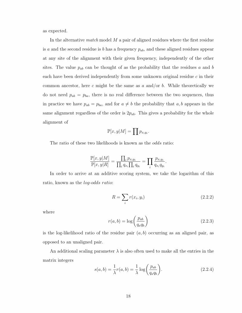
In the alternative match model M a pair of aligned residues where the first residue

is a and the second residue is b has a frequency pab, and these aligned residues appear

at any site of the alignment with their given frequency, independently of the other

sites. The value pab can be thought of as the probability that the residues a and b

each have been derived independently from some unknown original residue c in their

common ancestor, here c might be the same as a and/or b. While theoretically we

do not need pab = pba, there is no real difference between the two sequences, thus

in practice we have pab = pba, and for a 6= b the probability that a, b appears in the

same alignment regardless of the order is 2pab. This gives a probability for the whole

alignment of

P[x, y|M ] =∏

pxiyi .

The ratio of these two likelihoods is known as the odds ratio:

P[x, y|M ]

P[x, y|R]=

∏i pxiyi∏

i qxi∏

i qyi=∏i

pxiyiqxiqyi

.

In order to arrive at an additive scoring system, we take the logarithm of this

ratio, known as the log-odds ratio:

R =∑i

r(xi, yi) (2.2.2)

where

r(a, b) = log

(pabqaqb

)(2.2.3)

is the log-likelihood ratio of the residue pair (a, b) occurring as an aligned pair, as

opposed to an unaligned pair.

An additional scaling parameter λ is also often used to make all the entries in the

matrix integers

s(a, b) =1

λr(a, b) =

1

λlog

(pabqaqb

). (2.2.4)

18

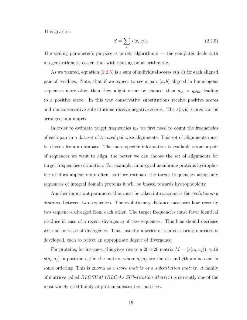
This gives us

S =∑i

s(xi, yi). (2.2.5)

The scaling parameter’s purpose is purely algorithmic — the computer deals with

integer arithmetic easier than with floating point arithmetic.

As we wanted, equation (2.2.5) is a sum of individual scores s(a, b) for each aligned

pair of residues. Note, that if we expect to see a pair (a, b) aligned in homologous

sequences more often then they might occur by chance, then pab > qaqb, leading

to a positive score. In this way conservative substitutions receive positive scores

and nonconservative substitutions receive negative scores. The s(a, b) scores can be

arranged in a matrix.

In order to estimate target frequencies pab we first need to count the frequencies

of each pair in a dataset of trusted pairwise alignments. This set of alignments must

be chosen from a database. The more specific information is available about a pair

of sequences we want to align, the better we can choose the set of alignments for

target frequencies estimation. For example, in integral membrane proteins hydropho-

bic residues appear more often, so if we estimate the target frequencies using only

sequences of integral domain proteins it will be biased towards hydrophobicity.

Another important parameter that must be taken into account is the evolutionary

distance between two sequences. The evolutionary distance measures how recently

two sequences diverged from each other. The target frequencies must favor identical

residues in case of a recent divergence of two sequences. This bias should decrease

with an increase of divergence. Thus, usually a series of related scoring matrices is

developed, each to reflect an appropriate degree of divergence.

For proteins, for instance, this gives rise to a 20× 20 matrix M = (s(ai, aj)), with

s(ai, aj) in position i, j in the matrix, where ai, aj are the ith and jth amino acid in

some ordering. This is known as a score matrix or a substitution matrix. A family

of matrices called BLOSUM (BLOcks SUbstitution Matrix) is currently one of the

most widely used family of protein substitution matrices.

19

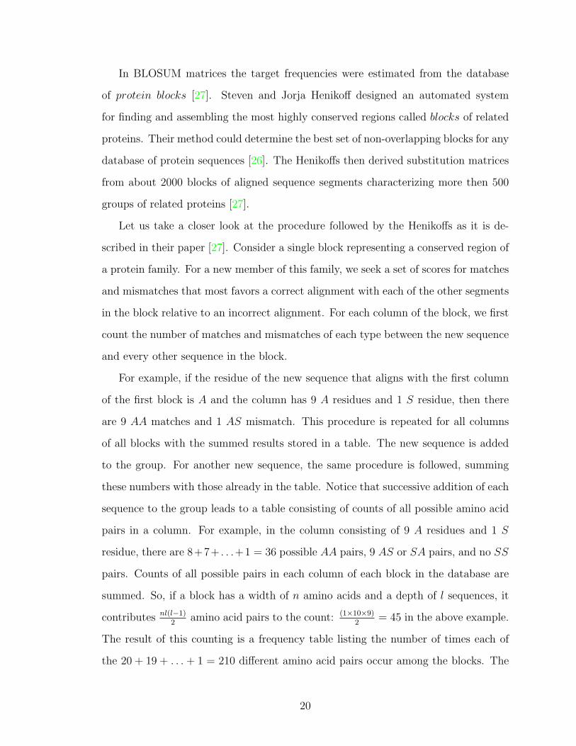
In BLOSUM matrices the target frequencies were estimated from the database

of protein blocks [27]. Steven and Jorja Henikoff designed an automated system

for finding and assembling the most highly conserved regions called blocks of related

proteins. Their method could determine the best set of non-overlapping blocks for any

database of protein sequences [26]. The Henikoffs then derived substitution matrices

from about 2000 blocks of aligned sequence segments characterizing more then 500

groups of related proteins [27].

Let us take a closer look at the procedure followed by the Henikoffs as it is de-

scribed in their paper [27]. Consider a single block representing a conserved region of

a protein family. For a new member of this family, we seek a set of scores for matches

and mismatches that most favors a correct alignment with each of the other segments

in the block relative to an incorrect alignment. For each column of the block, we first

count the number of matches and mismatches of each type between the new sequence

and every other sequence in the block.

For example, if the residue of the new sequence that aligns with the first column

of the first block is A and the column has 9 A residues and 1 S residue, then there

are 9 AA matches and 1 AS mismatch. This procedure is repeated for all columns

of all blocks with the summed results stored in a table. The new sequence is added

to the group. For another new sequence, the same procedure is followed, summing

these numbers with those already in the table. Notice that successive addition of each

sequence to the group leads to a table consisting of counts of all possible amino acid

pairs in a column. For example, in the column consisting of 9 A residues and 1 S

residue, there are 8+7+ . . .+1 = 36 possible AA pairs, 9 AS or SA pairs, and no SS

pairs. Counts of all possible pairs in each column of each block in the database are

summed. So, if a block has a width of n amino acids and a depth of l sequences, it

contributes nl(l−1)2

amino acid pairs to the count: (1×10×9)2

= 45 in the above example.

The result of this counting is a frequency table listing the number of times each of

the 20 + 19 + . . . + 1 = 210 different amino acid pairs occur among the blocks. The

20

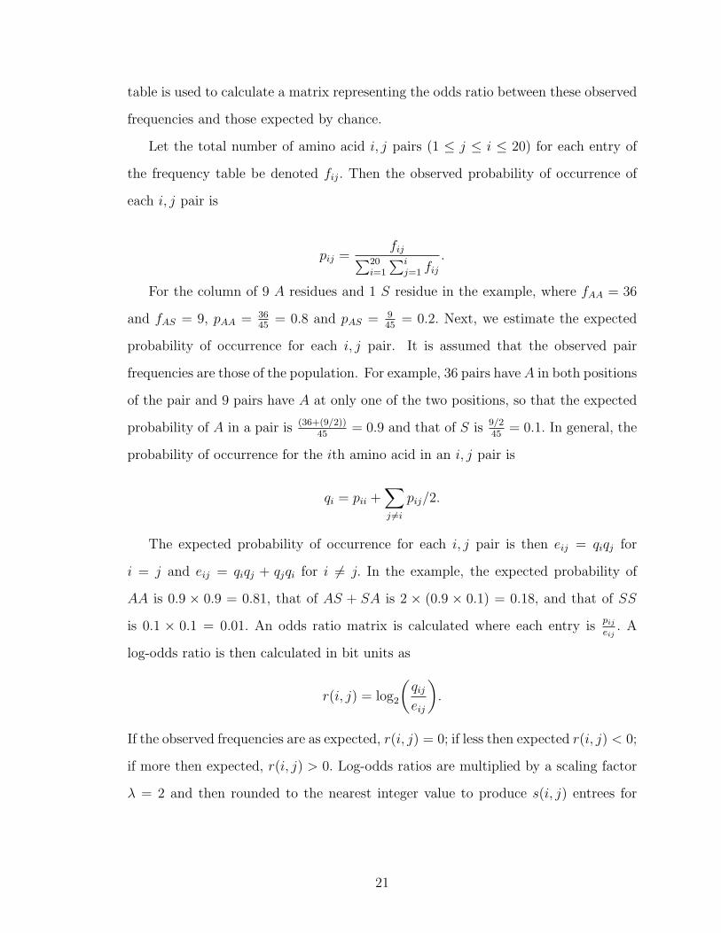
table is used to calculate a matrix representing the odds ratio between these observed

frequencies and those expected by chance.

Let the total number of amino acid i, j pairs (1 ≤ j ≤ i ≤ 20) for each entry of

the frequency table be denoted fij. Then the observed probability of occurrence of

each i, j pair is

pij =fij∑20

i=1

∑ij=1 fij

.

For the column of 9 A residues and 1 S residue in the example, where fAA = 36

and fAS = 9, pAA = 3645

= 0.8 and pAS = 945

= 0.2. Next, we estimate the expected

probability of occurrence for each i, j pair. It is assumed that the observed pair

frequencies are those of the population. For example, 36 pairs have A in both positions

of the pair and 9 pairs have A at only one of the two positions, so that the expected

probability of A in a pair is (36+(9/2))45

= 0.9 and that of S is 9/245

= 0.1. In general, the

probability of occurrence for the ith amino acid in an i, j pair is

qi = pii +∑j 6=i

pij/2.

The expected probability of occurrence for each i, j pair is then eij = qiqj for

i = j and eij = qiqj + qjqi for i 6= j. In the example, the expected probability of

AA is 0.9 × 0.9 = 0.81, that of AS + SA is 2 × (0.9 × 0.1) = 0.18, and that of SS

is 0.1 × 0.1 = 0.01. An odds ratio matrix is calculated where each entry ispijeij. A

log-odds ratio is then calculated in bit units as

r(i, j) = log2

(qijeij

).

If the observed frequencies are as expected, r(i, j) = 0; if less then expected r(i, j) < 0;

if more then expected, r(i, j) > 0. Log-odds ratios are multiplied by a scaling factor

λ = 2 and then rounded to the nearest integer value to produce s(i, j) entrees for

21

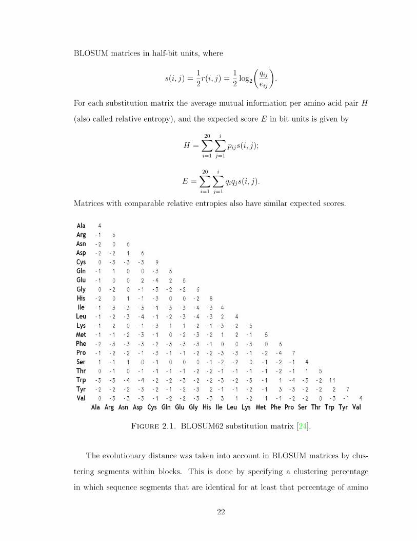
BLOSUM matrices in half-bit units, where

s(i, j) =1

2r(i, j) =

1

2log2

(qijeij

).

For each substitution matrix the average mutual information per amino acid pair H

(also called relative entropy), and the expected score E in bit units is given by

H =20∑i=1

i∑j=1

pijs(i, j);

E =20∑i=1

i∑j=1

qiqjs(i, j).

Matrices with comparable relative entropies also have similar expected scores.

Figure 2.1. BLOSUM62 substitution matrix [24].

The evolutionary distance was taken into account in BLOSUM matrices by clus-

tering segments within blocks. This is done by specifying a clustering percentage

in which sequence segments that are identical for at least that percentage of amino

22

acids are grouped together. In this way, varying the clustering percentage leads to

a family of BLOSUM matrices: BLOSUM80, BLOSUM70, BLOSUM62, and BLO-

SUM45. For example, to construct BLOSUM62 percentage of 62% is used. Clustering

at 62% reduces the number of blocks contributing to the table by 25% with the re-

mainder contributing 1.25 million pairs (including fractional pairs), whereas without

clustering, > 15 million pairs are counted.

Henikoffs were able to show that BLOSUM matrices perform better then other

general purpose substitution matrices. They chose a group of protein sequences called

the guanine nucleotide-binding protein-coupled receptors. This particularly challeng-

ing group had been previously used to test searching and alignment programs. From

114 family members three distinct sequences were chosen for queries. Henikoffs per-

formed these queries against the PROSITE 8.0 database, a database of protein fam-

ilies and domains [28], using BLOSUM and other matrices. They showed that when

performing search using BLOSUM matrices more sequences from the target group

could be detected [27]. They also conducted similar study for other 504 protein

groups stored in PROSITE 8.0 database and showed that BLOSUM62 performed

slightly better then other BLOSUM matrices [27].

It is also important to keep in mind that the scoring is based on log-odds ratios, not

just the frequencies of observed aligned pairs. For example, in a substitution matrix

BLOSUM62, if we compare identity scores for tryptophan (W) and leucine (L) pairs,

we see that they are considerably different s(W,W ) = 11, and s(L,L) = 4. At first

glance, this might seem counterintuitive, since in the BLOSUM62 training dataset

the estimated target frequencies for leucine and tryptophan were pLL = 0.0371 and

pWW = 0.0065. However, statistically tryptophan is a much rarer amino acid then

leucine, more precisely, qW = 0.013 and qL = 0.099. So, we get

s(W,W ) =1

0.347ln

(0.0065

0.0132

)= 10.5,

and

23

s(L,L) =1

0.347ln

(0.0371

0.0992

)= 3.8,

where λ = 0.347 is the scaling parameter. In the BLOSUM62 matrix these scores are

rounded to s(W,W ) = 11, and s(L,L) = 4 [19].

2.2.4. Gap Penalties. There is no general theory available for guiding the

choice of gap costs. The scoring of gaps were usually chosen with two things in

mind: one, that the resulting algorithms that compute the alignments and scores are

effective, the other, that the resulting alignments are reasonable.

The most straightforward scheme is to charge a fixed penalty for each indel, i.e.,

∆CONST (k) = dk

for a gap of length k, d = const. However, biologically, a gap of length k > 1 is more

likely to happen than k gaps of length 1. This is because a single mutational event

usually results in insertion or deletion of a stretch of characters. Moreover, separated

gaps are due to distinct mutational events and by the previous argument tend to be

longer. Over the years, it has been observed that the optimal alignments produced by

the constant gap scheme usually contain a large number of short gaps and are often

not biologically meaningful.

To capture the idea that a single mutational event might insert or delete a sequence

of residues, Waterman and Smith [41] introduced the affine gap penalty model. Under

this model, the penalty

∆AFF (k) = o+ ek

is charged for a gap of length k ≥ 1, where o is a large penalty for opening a gap and

e a smaller penalty for extending it.

The affine gap cost is based on the hypothesis that gap length has an exponential

distribution, that is, the probability of a gap of length k ≥ 1 is α(1− β)βk for some

constants α and β. Under this hypothesis, an affine gap cost is derived by charging

24

log(α(1−β)βk) for a gap of length k. But this hypothesis might not be true in general.

For instance the study of Benner, Cohen, and Gonnet [9] suggests that the frequency

of a length k is accurately discribed by mk−1.7 for some constant m, i.e., a power law.

A generalized affine gap cost is introduced by Altschul [1]. A generalized gap

consists of a consecutive sequence of indels in which spaces can be in either row. A

generalized gap of length 10 may contain 10 insertions; it may also contain 4 insertions

and 6 deletions. To reflect the structural property of a generalized gap, a generalized

affine gap cost has three parameters a, b, c. The score −a is introduced for the opening

of a gap; −b is for each residue inserted or deleted; and −c is for each pair of residues

left unaligned. For a gap with k ≥ 0 insertions and l ≥ 0 deletions such that k+` ≥ 1

a generalized gap penalty is

∆GEN(k, `) = −(a+ |k − `|b) + cmink, `.

Generalized affine gap costs can be used for locally or globally aligning protein

sequences. The empirical study of Zachariah et al. [49] shows that this generalized

affine gap cost model improves significantly the accuracy of protein alignment.

Sometimes it is more convenient to think of an alignment in the following way

D I H H H I H D H

A =



.

The additional line of letters H,D, I, where H, I, D stand for homology, in-

sertion, and deletion, denotes each column by its type. With this representation in

mind it is more convenient to organize gap penalties in a matrix. Consider a 3 × 3

matrix

W =

w(I, I) w(I,H) w(I,D)

w(H, I) w(H,H) w(H,D)

w(D, I) w(D,H) w(D,D)

,

25

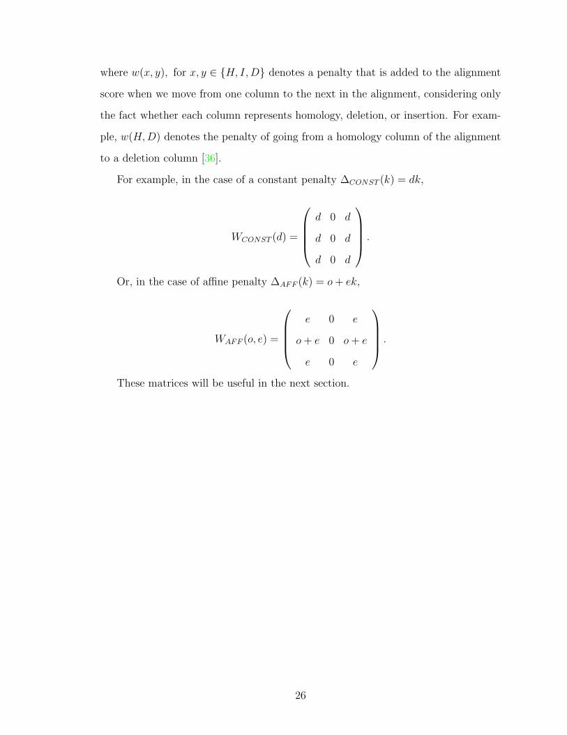
where w(x, y), for x, y ∈ H, I,D denotes a penalty that is added to the alignment

score when we move from one column to the next in the alignment, considering only

the fact whether each column represents homology, deletion, or insertion. For exam-

ple, w(H,D) denotes the penalty of going from a homology column of the alignment

to a deletion column [36].

For example, in the case of a constant penalty ∆CONST (k) = dk,

WCONST (d) =

d 0 d

d 0 d

d 0 d

.

Or, in the case of affine penalty ∆AFF (k) = o+ ek,

WAFF (o, e) =

e 0 e

o+ e 0 o+ e

e 0 e

.

These matrices will be useful in the next section.

26

2.3. Alignment Algorithms

2.3.1. Computational Perspective. Once we set a proper scoring scheme, de-

ciding that two biological sequences are similar is no different from deciding that

two text strings are similar. One set of methods for biological sequence analysis is

therefore rooted in computer science, where there is an extensive literature on string

comparison methods [18].

Definition 15. The alignment graph Gn,m is the directed graph on the set of nodes

0, 1, . . . , n × 0, 1, . . . ,m and three classes of directed edges as follows:

• (diagonal) edges labeled by S between pairs of nodes (i, j) → (i + 1, j + 1),

where 0 ≤ i ≤ n− 1 and 0 ≤ j ≤ m− 1;

• (horizontal) edges labeled by I between pairs of nodes (i, j) → (i, j + 1),

where 0 ≤ i ≤ n and 0 ≤ j ≤ m− 1;

• (vertical) edges labeled by D between pairs of nodes (i, j)→ (i+1, j), where

0 ≤ i ≤ n− 1 and 0 ≤ j ≤ m [36].

An alignment graph together with vertex (0, 0) as a source and vertex (n,m) as

a sink forms an alignment network.

All possible alignments correspond one-to-one to the directed paths from the

source to the sink in the alignment network. Thus, the alignment network gives

a compact representation of all possible alignments of the sequences. The alignments

of two sequences of length n and m and the directed paths from source to sink in the

alignment graph Gn,m are in one-to-one correspondence with each other. A diagonal

edge of the form (i − 1, j − 1) → (i, j) corresponds to a site where the i-th letter of

the first sequence is aligned with the j-th letter of the second sequence, and horizon-

tal/vertical edges of the form (i− 1, j − 1)→ (i− 1, j) and (i− 1, j − 1)→ (i, j − 1)

correspond to a − being aligned with the j-th letter of the second sequence or the

i-th letter of the first sequence, respectively. Thus, the alignment network gives a

compact representation of all possible alignments of the two sequences. Figure 2.2

27

TGCCT GG

GGTCATA

0 654321

7

7

0

1

2

3

4

5

6

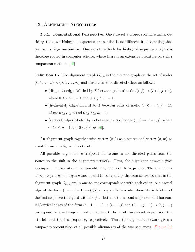
Figure 2.2. Aligment graph for sequences ATACTGG and GTC-CGTG [10].

shows an example from [10], where Σ = A,C,G, T, n = m = 7, X = ATACTGG,

Y = GTCCGTG, and the highlighted path in the alignment network is

PA = (0, 0)→ (1, 0)→ (1, 1)→ (2, 2)→ (3, 3)→ (4, 4)→ (4, 5)→ (5, 6)→ (6, 6)

→ (7, 7).

This path represents the following alignment

A =



28

TGCCT GG

GGTCATA

0 654321

7

7

0

1

2

3

4

5

6

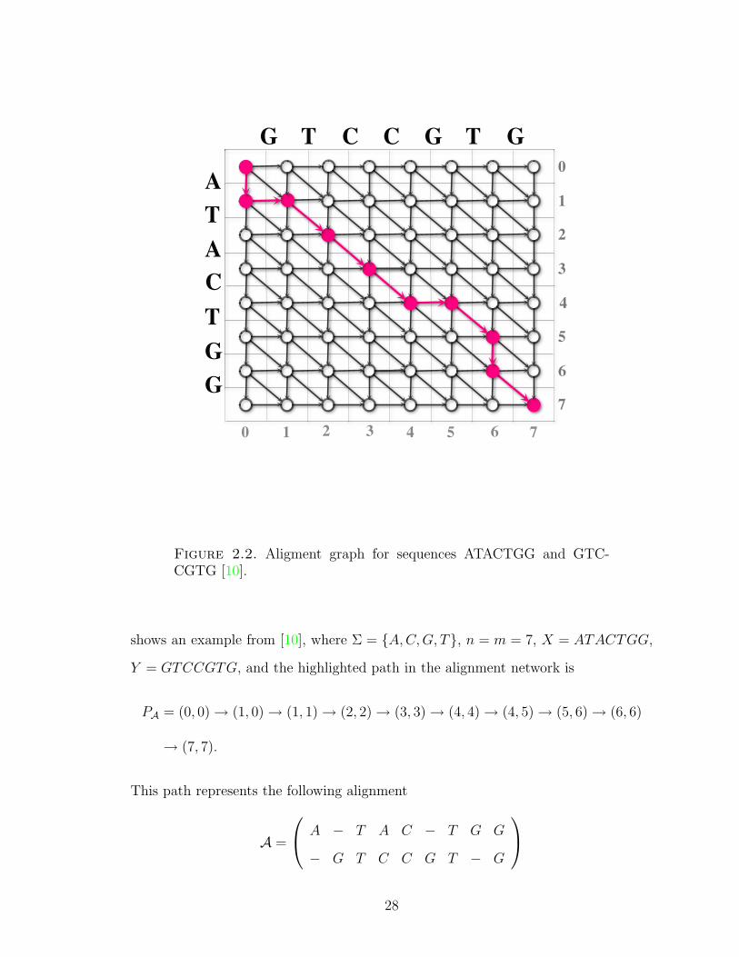
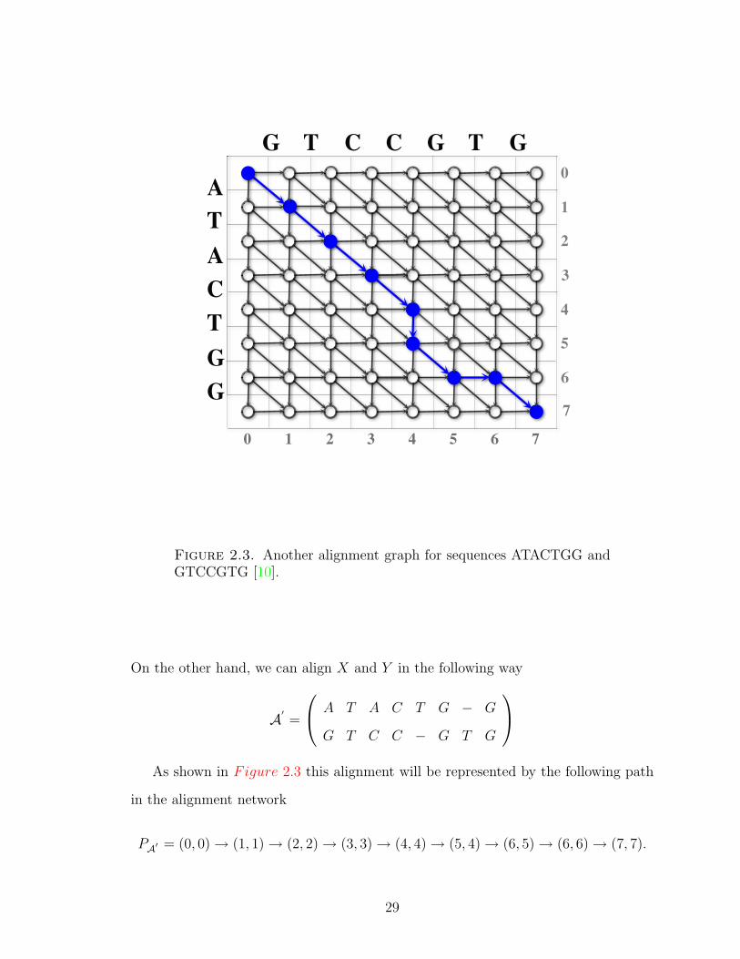
Figure 2.3. Another alignment graph for sequences ATACTGG andGTCCGTG [10].

On the other hand, we can align X and Y in the following way

A′ =

A T A C T G − G

G T C C − G T G

As shown in Figure 2.3 this alignment will be represented by the following path

in the alignment network

PA′ = (0, 0)→ (1, 1)→ (2, 2)→ (3, 3)→ (4, 4)→ (5, 4)→ (6, 5)→ (6, 6)→ (7, 7).

29

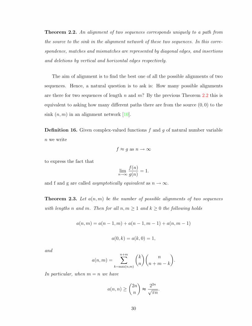
Theorem 2.2. An alignment of two sequences corresponds uniquely to a path from

the source to the sink in the alignment network of these two sequences. In this corre-

spondence, matches and mismatches are represented by diagonal edges, and insertions

and deletions by vertical and horizontal edges respectively.

The aim of alignment is to find the best one of all the possible alignments of two

sequences. Hence, a natural question is to ask is: How many possible alignments

are there for two sequences of length n and m? By the previous Theorem 2.2 this is

equivalent to asking how many different paths there are from the source (0, 0) to the

sink (n,m) in an alignment network [10].

Definition 16. Given complex-valued functions f and g of natural number variable

n we write

f ≈ g as n→∞

to express the fact that

limn→∞

f(n)

g(n)= 1.

and f and g are called asymptotically equivalent as n→∞.

Theorem 2.3. Let a(n,m) be the number of possible alignments of two sequences

with lengths n and m. Then for all n,m ≥ 1 and k ≥ 0 the following holds

a(n,m) = a(n− 1,m) + a(n− 1,m− 1) + a(n,m− 1)

a(0, k) = a(k, 0) = 1,

and

a(n,m) =n+m∑

k=max(n,m)

(k

n

)(n

n+m− k

).

In particular, when m = n we have

a(n, n) ≥(

2n

n

)≈

22n

√πn

.

30

Proof. In an alignment network the paths from the source (0, 0) to a vertex (i, j)

correspond to possible alignments of two sequences of length i and j. Hence, a(i, j)

is equal to the number of paths from (0, 0) to the vertex (i, j). Because every path

from the source (0, 0) to the sink (m,n) must go through exactly one of the vertices

(m− 1, n), (m,n− 1), and (n− 1,m− 1), we obtain a(n,m) = a(n− 1,m) + a(n−

1,m− 1) + a(n,m− 1).

There is only one way to align the empty sequence to a non-empty sequence. Thus

for any k ≥ 0 we have a(0, k) = a(k, 0) = 1.

Suppose there are k columns in the alignment with n letters and k − n spaces in

the first row and m letters and k − m spaces the second row. This means that we

must have min(n,m) ≤ k, since the number of columns in the alignment is at least

as much as the length of the longer sequence, and k ≤ m + n, since for more than

m + n columns we should have two spaces aligned, which is not allowed.There are(kn

)possible ways to arrange the n letters in the first row. For each such arrangement

k − m spaces in the second row must be placed below the letters in the first row

giving(

nk−m

)=(

nn+m−k

)possible arrangements. Thus we have ak(n,m) =

(kn

)(n

n+m−k

)possible k-column alignments. Since max(n,m) ≤ k ≤ m + n the number of all

possible alignments of two sequences with lengths n and m can be calculated by the

formula

a(n,m) =n+m∑

k=max(n,m)

(k

n

)(n

n+m− k

).

In case n = m we have

a(n, n) =2n∑k=n

(k

n

)(n

2n− k

)=

2n−1∑k=n

(k

n

)(n

2n− k

)+

(2n

n

)≥(

2n

n

).

Applying Stirling’s approximation

x! ≈√

2πxx+ 12 e−x,

31

we obtain

a(n, n) ≥(

2n

n

)≈ 22n

√πn

as desired [10].

For example consider two sequences of length 100. By Theorem 2.3 we have

a(100, 100) > 2196 > 1059, an astronomically large number. Clearly, this shows that

it is definitely not feasible to examine all possible alignments and that we need an

efficient method for sequence alignment.

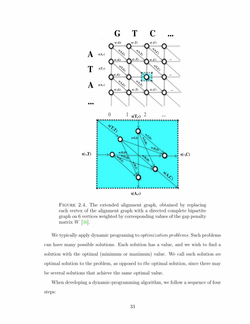
To take gap penalties into account we generalize the notion of an alignment graph

to an extended alignment graph which is a graph obtained by replacing each vertex

in the alignment graph with a directed complete bipartite graph on 6 vertices with

edges weighted by corresponding values of a gap penalty matrix W. This procedure

is shown in detail in Figure 2.4.

An extended alignment graph weighted according to a scoring scheme with vertices

(0, 0) as a source and (n,m) as a sink forms an extended alignment network.

With an appropriate scoring scheme used to weigh the corresponding edges of

an alignment network, finding an alignment with maximum score, i.e., an optimal

alignment is equivalent to finding a directed path of maximum length in the extended

alignment network.

2.3.2. Dynamic Programming. Recall that, while searching for an optimal

alignment, we can not simply compute all possible alignments, due to the fact that

their number is quite large. Thus, there is a need for an efficient computational

method. One such method is known as dynamic programming.

The dynamic-programming paradigm applies when subproblems overlap — that

is, when subproblems share subproblems. A dynamic-programming algorithm solves

each subproblem just once and then saves its answer in a table, thereby avoiding the

work of recomputing the answer every time it solves each subproblem.

32

w(H,H)

w(D,D)

s(T,T)

s(A,C)

w(I,H

)

w(I,D)

w(H,D)

w(H,I)

w(D,H)w(D,I)

s(T,-)

s(-,T)

s(A,-)

s(-,C)

w(I,I)

...

...

...

s(A,G)

s(A,G)

s(T,G)

s(A,C)s(A,T)

s(T,C)

s(A,T)

...CTG

A

TA

0 ...21

...

s(-,G)

s(A,-)

s(T,-)

s(A,-)

s(-,G)

s(-,G)

s(-,T) s(-,C)

s(-,T)

s(-,C)

s(-,C)

s(-,T)s(-,G)

Figure 2.4. The extended alignment graph, obtained by replacingeach vertex of the alignment graph with a directed complete bipartitegraph on 6 vertices weighted by corresponding values of the gap penaltymatrix W [36].

We typically apply dynamic programing to optimization problems. Such problems

can have many possible solutions. Each solution has a value, and we wish to find a

solution with the optimal (minimum or maximum) value. We call such solution an

optimal solution to the problem, as opposed to the optimal solution, since there may

be several solutions that achieve the same optimal value.

When developing a dynamic-programming algorithm, we follow a sequence of four

steps:

33

1. Characterize the structure of an optimal solution.

2. Recursively define the value of an optimal solution.

3. Compute the value of an optimal solution, typically in a botton-up fashion.

4. Construct an optimal solution from the computed information.

Steps 1 − 3 form the basis of a dynamic-programming solution to a problem. If

we need only the value of an optimal solution, and not the solution itself, then we

can omit step 4. When we do perform step 4, we sometimes maintain additional

information during step 3 so that we can easily construct an optimal solution [13].

In the case of optimal sequence alignment a dynamic-programming algorithm in

general follows a sequence of three steps:

1. An initialization of dynamic-programming matrix (or matrices) for remem-

bering optimal scores of subproblems.

2. A recursive definition of the optimal score and a bottom-up approach of

filling the matrix by solving the smallest subproblems first.

3. A backtracking procedure to recover the structure of the optimal solution

that gave the optimal score. This procedure is often called a traceback in

standard literature [13].

2.3.3. Global Pairwise Alignment. We first consider a problem of the op-

timal global alignment between two sequences with gaps. The Needleman-Wunsch

algorithm [34] is a standard dynamic-programming algorithm for solving this problem.

A more efficient version was later introduced by Gotoh [22].

We want to build an optimal gapped alignment with constant gap penalty δ(k) =

dk using previous solutions for optimal alignments of smaller subsequences. Suppose

we are aligning two sequences X = x1 . . . xn and Y = y1 . . . ym, S is an (n+1)×(m+1)

matrix indexed by (i, j), and S(i, j) is the score of the best possible alignment between

initial segments x1 . . . xi and y1 . . . yj. We can define a recursion for building S(i, j).

34

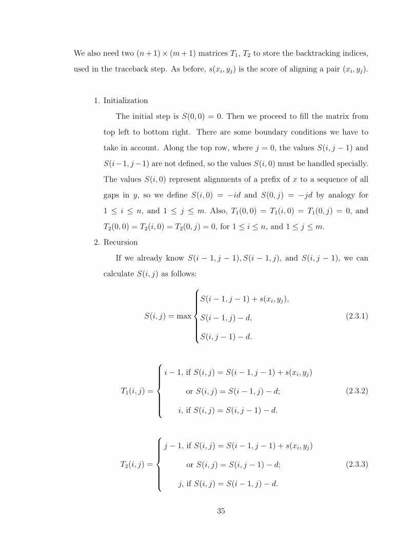
We also need two (n+ 1)× (m+ 1) matrices T1, T2 to store the backtracking indices,

used in the traceback step. As before, s(xi, yj) is the score of aligning a pair (xi, yj).

1. Initialization

The initial step is S(0, 0) = 0. Then we proceed to fill the matrix from

top left to bottom right. There are some boundary conditions we have to

take in account. Along the top row, where j = 0, the values S(i, j − 1) and

S(i−1, j−1) are not defined, so the values S(i, 0) must be handled specially.

The values S(i, 0) represent alignments of a prefix of x to a sequence of all

gaps in y, so we define S(i, 0) = −id and S(0, j) = −jd by analogy for

1 ≤ i ≤ n, and 1 ≤ j ≤ m. Also, T1(0, 0) = T1(i, 0) = T1(0, j) = 0, and

T2(0, 0) = T2(i, 0) = T2(0, j) = 0, for 1 ≤ i ≤ n, and 1 ≤ j ≤ m.

2. Recursion

If we already know S(i − 1, j − 1), S(i − 1, j), and S(i, j − 1), we can

calculate S(i, j) as follows:

S(i, j) = max

S(i− 1, j − 1) + s(xi, yj),

S(i− 1, j)− d,

S(i, j − 1)− d.

(2.3.1)

T1(i, j) =

i− 1, if S(i, j) = S(i− 1, j − 1) + s(xi, yj)

or S(i, j) = S(i− 1, j)− d;

i, if S(i, j) = S(i, j − 1)− d.

(2.3.2)

T2(i, j) =

j − 1, if S(i, j) = S(i− 1, j − 1) + s(xi, yj)

or S(i, j) = S(i, j − 1)− d;

j, if S(i, j) = S(i− 1, j)− d.

(2.3.3)

35

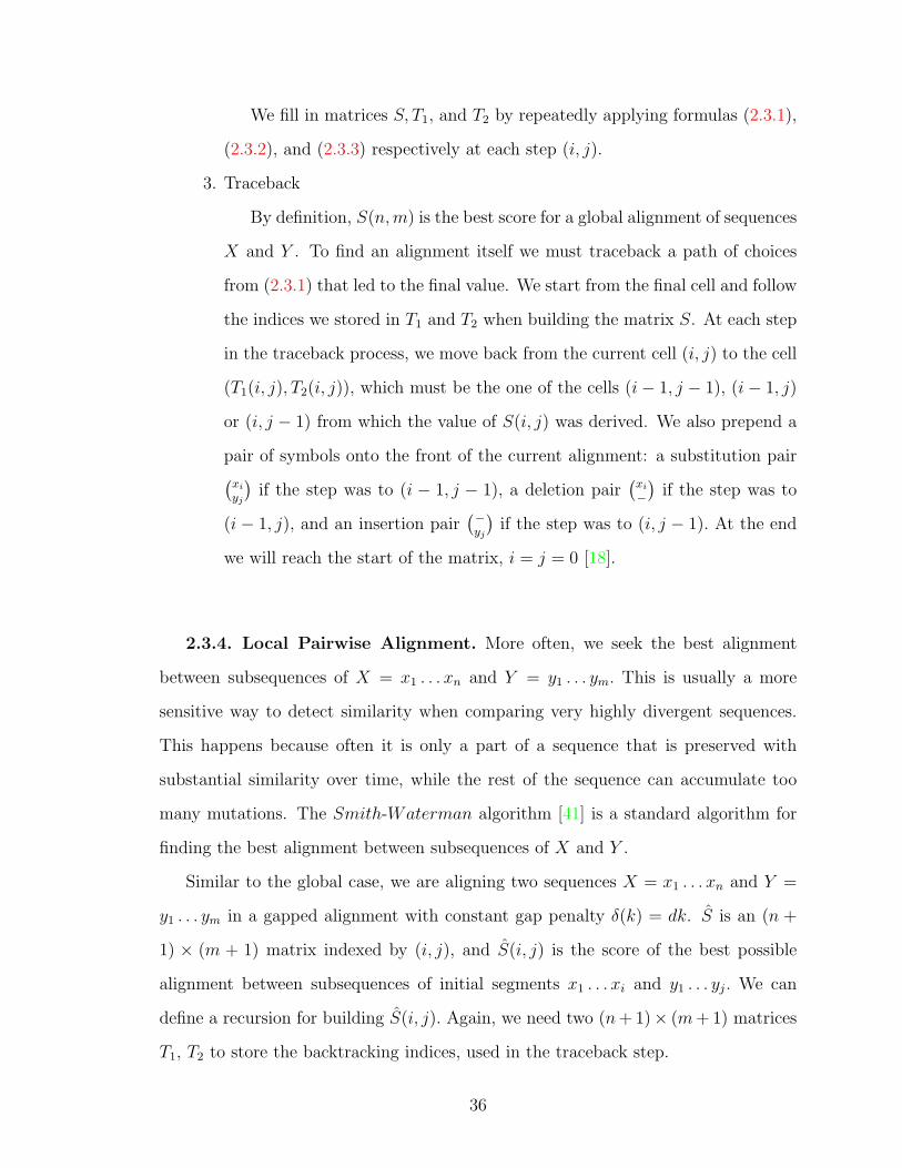
We fill in matrices S, T1, and T2 by repeatedly applying formulas (2.3.1),

(2.3.2), and (2.3.3) respectively at each step (i, j).

3. Traceback

By definition, S(n,m) is the best score for a global alignment of sequences

X and Y . To find an alignment itself we must traceback a path of choices

from (2.3.1) that led to the final value. We start from the final cell and follow

the indices we stored in T1 and T2 when building the matrix S. At each step

in the traceback process, we move back from the current cell (i, j) to the cell

(T1(i, j), T2(i, j)), which must be the one of the cells (i− 1, j − 1), (i− 1, j)

or (i, j − 1) from which the value of S(i, j) was derived. We also prepend a

pair of symbols onto the front of the current alignment: a substitution pair(xiyj

)if the step was to (i − 1, j − 1), a deletion pair

(xi−

)if the step was to

(i − 1, j), and an insertion pair(−yj

)if the step was to (i, j − 1). At the end

we will reach the start of the matrix, i = j = 0 [18].

2.3.4. Local Pairwise Alignment. More often, we seek the best alignment

between subsequences of X = x1 . . . xn and Y = y1 . . . ym. This is usually a more

sensitive way to detect similarity when comparing very highly divergent sequences.

This happens because often it is only a part of a sequence that is preserved with

substantial similarity over time, while the rest of the sequence can accumulate too

many mutations. The Smith-Waterman algorithm [41] is a standard algorithm for

finding the best alignment between subsequences of X and Y .

Similar to the global case, we are aligning two sequences X = x1 . . . xn and Y =

y1 . . . ym in a gapped alignment with constant gap penalty δ(k) = dk. S is an (n +

1) × (m + 1) matrix indexed by (i, j), and S(i, j) is the score of the best possible

alignment between subsequences of initial segments x1 . . . xi and y1 . . . yj. We can

define a recursion for building S(i, j). Again, we need two (n+ 1)× (m+ 1) matrices

T1, T2 to store the backtracking indices, used in the traceback step.

36

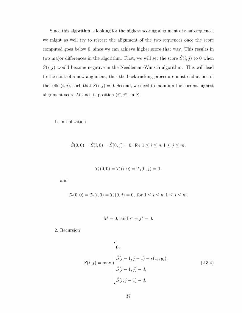
Since this algorithm is looking for the highest scoring alignment of a subsequence,

we might as well try to restart the alignment of the two sequences once the score

computed goes below 0, since we can achieve higher score that way. This results in

two major differences in the algorithm. First, we will set the score S(i, j) to 0 when

S(i, j) would become negative in the Needleman-Wunsch algorithm. This will lead

to the start of a new alignment, thus the backtracking procedure must end at one of

the cells (i, j), such that S(i, j) = 0. Second, we need to maintain the current highest

alignment score M and its position (i?, j?) in S.

1. Initialization

S(0, 0) = S(i, 0) = S(0, j) = 0, for 1 ≤ i ≤ n, 1 ≤ j ≤ m.

T1(0, 0) = T1(i, 0) = T1(0, j) = 0,

and

T2(0, 0) = T2(i, 0) = T2(0, j) = 0, for 1 ≤ i ≤ n, 1 ≤ j ≤ m.

M = 0, and i? = j? = 0.

2. Recursion

S(i, j) = max

0,

S(i− 1, j − 1) + s(xi, yj),

S(i− 1, j)− d,

S(i, j − 1)− d.

(2.3.4)

37

T1(i, j) =

i− 1, if S(i, j) = S(i− 1, j − 1) + s(xi, yj)

or S(i, j) = S(i− 1, j)− d;

i, if S(i, j) = S(i, j − 1)− d

or S(i, j) = 0.

(2.3.5)

T2(i, j) =

j − 1, if S(i, j) = S(i− 1, j − 1) + s(xi, yj)

or S(i, j) = S(i, j − 1)− d;

j, if S(i, j) = S(i− 1, j)− d

or S(i, j) = 0.

(2.3.6)

(i?, j?) =

(i, j), if S(i, j) > M ;

remains unchanged otherwise .(2.3.7)

M =

S(i, j), if S(i, j) > M ;


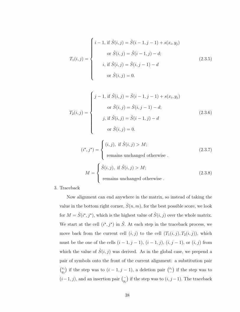
3. Traceback

Now alignment can end anywhere in the matrix, so instead of taking the

value in the bottom right corner, S(n,m), for the best possible score, we look

for M = S(i?, j?), which is the highest value of S(i, j) over the whole matrix.

We start at the cell (i?, j?) in S. At each step in the traceback process, we

move back from the current cell (i, j) to the cell (T1(i, j), T2(i, j)), which

must be the one of the cells (i− 1, j − 1), (i− 1, j), (i, j − 1), or (i, j) from

which the value of S(i, j) was derived. As in the global case, we prepend a

pair of symbols onto the front of the current alignment: a substitution pair(xiyj


(xi−

)if the step was to

(i−1, j), and an insertion pair(−yj

)if the step was to (i, j−1). The traceback

38

ends if we move from (i, j) to (i, j), i.e. if we remain at the same position.

This means that we have reached a point where S(i, j) = 0, and our local

alignment started from here [18].

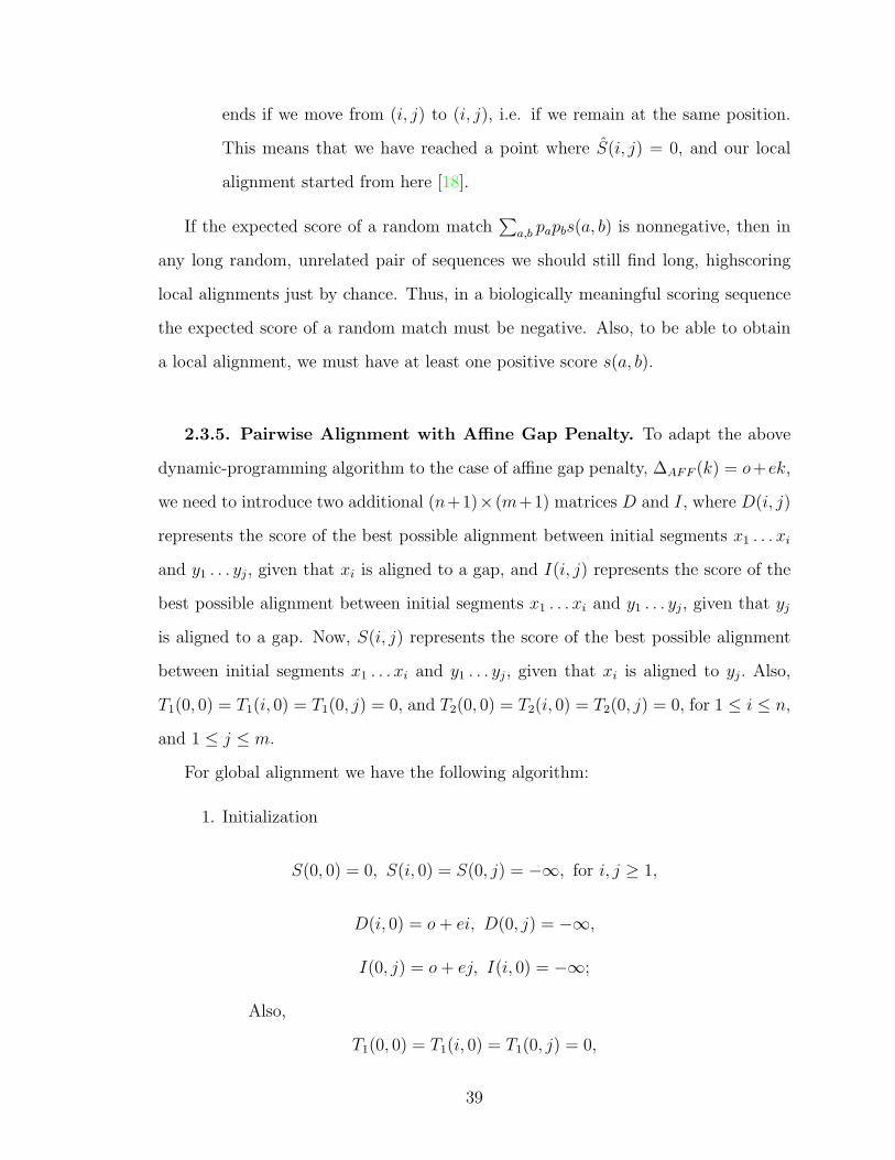
If the expected score of a random match∑

a,b papbs(a, b) is nonnegative, then in

any long random, unrelated pair of sequences we should still find long, highscoring

local alignments just by chance. Thus, in a biologically meaningful scoring sequence

the expected score of a random match must be negative. Also, to be able to obtain

a local alignment, we must have at least one positive score s(a, b).

2.3.5. Pairwise Alignment with Affine Gap Penalty. To adapt the above

dynamic-programming algorithm to the case of affine gap penalty, ∆AFF (k) = o+ek,

we need to introduce two additional (n+1)×(m+1) matrices D and I, where D(i, j)

represents the score of the best possible alignment between initial segments x1 . . . xi

and y1 . . . yj, given that xi is aligned to a gap, and I(i, j) represents the score of the

best possible alignment between initial segments x1 . . . xi and y1 . . . yj, given that yj

is aligned to a gap. Now, S(i, j) represents the score of the best possible alignment

between initial segments x1 . . . xi and y1 . . . yj, given that xi is aligned to yj. Also,

T1(0, 0) = T1(i, 0) = T1(0, j) = 0, and T2(0, 0) = T2(i, 0) = T2(0, j) = 0, for 1 ≤ i ≤ n,

and 1 ≤ j ≤ m.

For global alignment we have the following algorithm:

1. Initialization

S(0, 0) = 0, S(i, 0) = S(0, j) = −∞, for i, j ≥ 1,

D(i, 0) = o+ ei, D(0, j) = −∞,

I(0, j) = o+ ej, I(i, 0) = −∞;

Also,

T1(0, 0) = T1(i, 0) = T1(0, j) = 0,

39

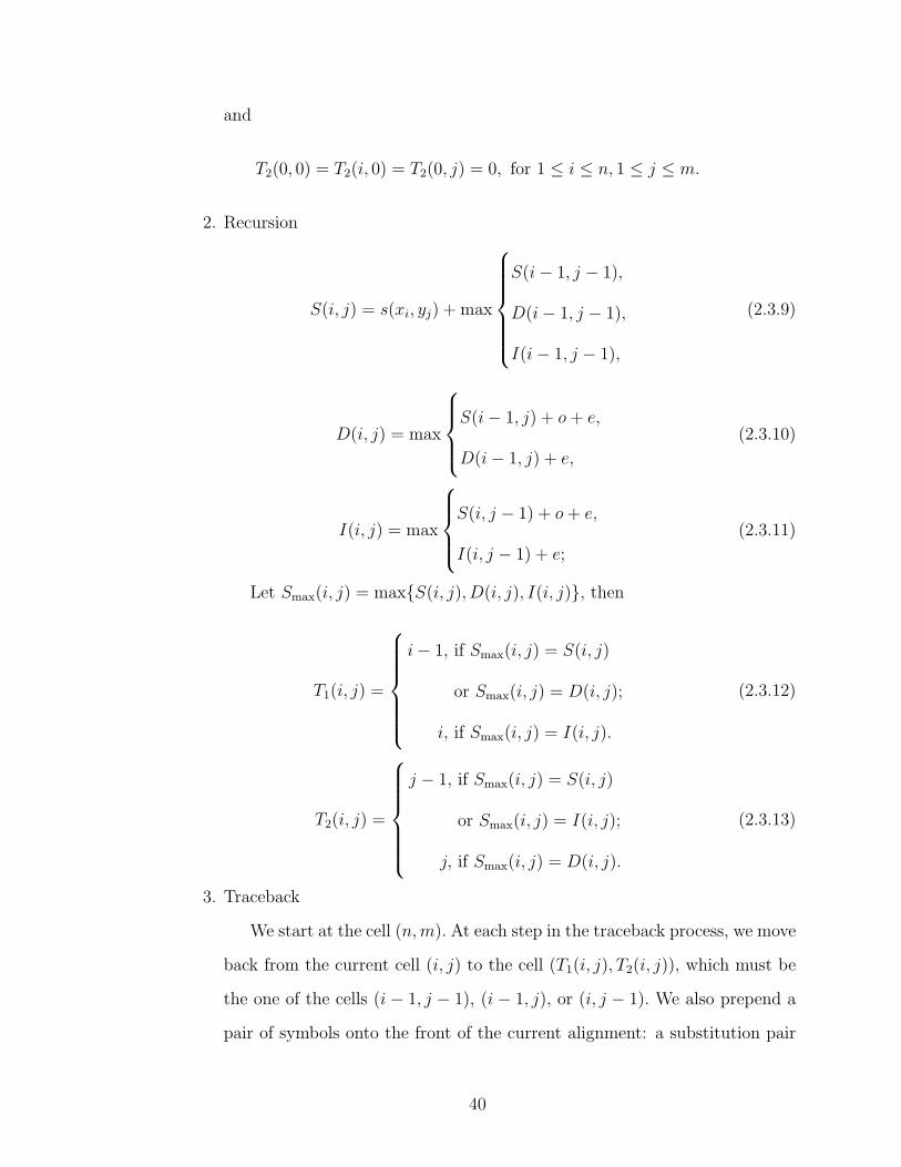
and

T2(0, 0) = T2(i, 0) = T2(0, j) = 0, for 1 ≤ i ≤ n, 1 ≤ j ≤ m.

2. Recursion

S(i, j) = s(xi, yj) + max

S(i− 1, j − 1),

D(i− 1, j − 1),

I(i− 1, j − 1),

(2.3.9)

D(i, j) = max

S(i− 1, j) + o+ e,

D(i− 1, j) + e,

(2.3.10)

I(i, j) = max

S(i, j − 1) + o+ e,

I(i, j − 1) + e;

(2.3.11)

Let Smax(i, j) = maxS(i, j), D(i, j), I(i, j), then

T1(i, j) =

i− 1, if Smax(i, j) = S(i, j)

or Smax(i, j) = D(i, j);

i, if Smax(i, j) = I(i, j).

(2.3.12)

T2(i, j) =

j − 1, if Smax(i, j) = S(i, j)

or Smax(i, j) = I(i, j);

j, if Smax(i, j) = D(i, j).

(2.3.13)

3. Traceback

We start at the cell (n,m). At each step in the traceback process, we move

back from the current cell (i, j) to the cell (T1(i, j), T2(i, j)), which must be

the one of the cells (i − 1, j − 1), (i − 1, j), or (i, j − 1). We also prepend a

pair of symbols onto the front of the current alignment: a substitution pair

40

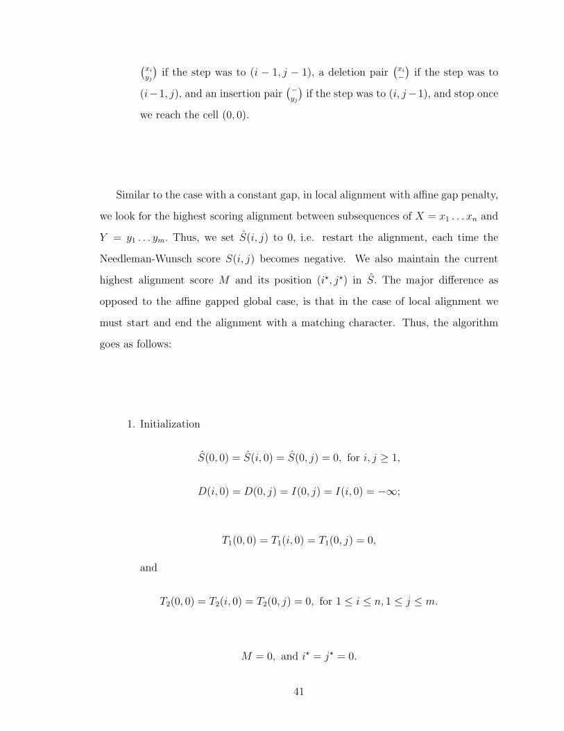
(xiyj


(xi−

)if the step was to

(i−1, j), and an insertion pair(−yj

)if the step was to (i, j−1), and stop once

we reach the cell (0, 0).

Similar to the case with a constant gap, in local alignment with affine gap penalty,

we look for the highest scoring alignment between subsequences of X = x1 . . . xn and

Y = y1 . . . ym. Thus, we set S(i, j) to 0, i.e. restart the alignment, each time the

Needleman-Wunsch score S(i, j) becomes negative. We also maintain the current

highest alignment score M and its position (i?, j?) in S. The major difference as

opposed to the affine gapped global case, is that in the case of local alignment we

must start and end the alignment with a matching character. Thus, the algorithm

goes as follows:

1. Initialization

S(0, 0) = S(i, 0) = S(0, j) = 0, for i, j ≥ 1,

D(i, 0) = D(0, j) = I(0, j) = I(i, 0) = −∞;

T1(0, 0) = T1(i, 0) = T1(0, j) = 0,

and

T2(0, 0) = T2(i, 0) = T2(0, j) = 0, for 1 ≤ i ≤ n, 1 ≤ j ≤ m.

M = 0, and i? = j? = 0.

41

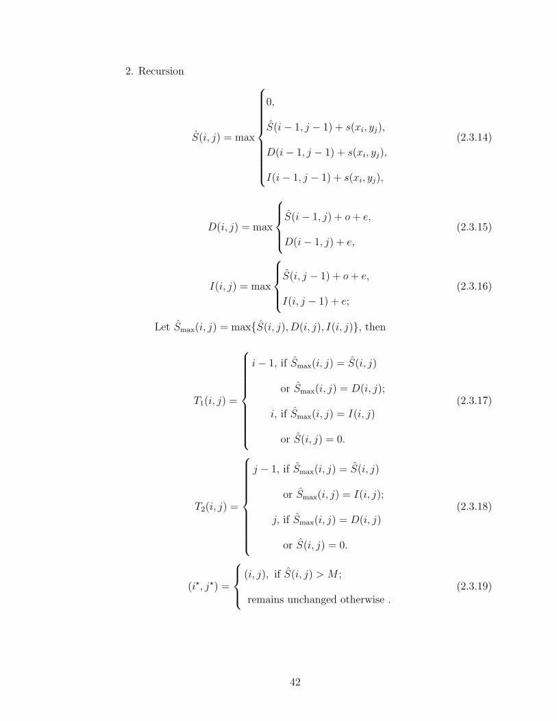
2. Recursion

S(i, j) = max

0,

S(i− 1, j − 1) + s(xi, yj),

D(i− 1, j − 1) + s(xi, yj),

I(i− 1, j − 1) + s(xi, yj),

(2.3.14)

D(i, j) = max

S(i− 1, j) + o+ e,

D(i− 1, j) + e,

(2.3.15)

I(i, j) = max

S(i, j − 1) + o+ e,

I(i, j − 1) + e;

(2.3.16)

Let Smax(i, j) = maxS(i, j), D(i, j), I(i, j), then

T1(i, j) =

i− 1, if Smax(i, j) = S(i, j)

or Smax(i, j) = D(i, j);

i, if Smax(i, j) = I(i, j)

or S(i, j) = 0.

(2.3.17)

T2(i, j) =

j − 1, if Smax(i, j) = S(i, j)

or Smax(i, j) = I(i, j);

j, if Smax(i, j) = D(i, j)

or S(i, j) = 0.

(2.3.18)

(i?, j?) =

(i, j), if S(i, j) > M ;


42

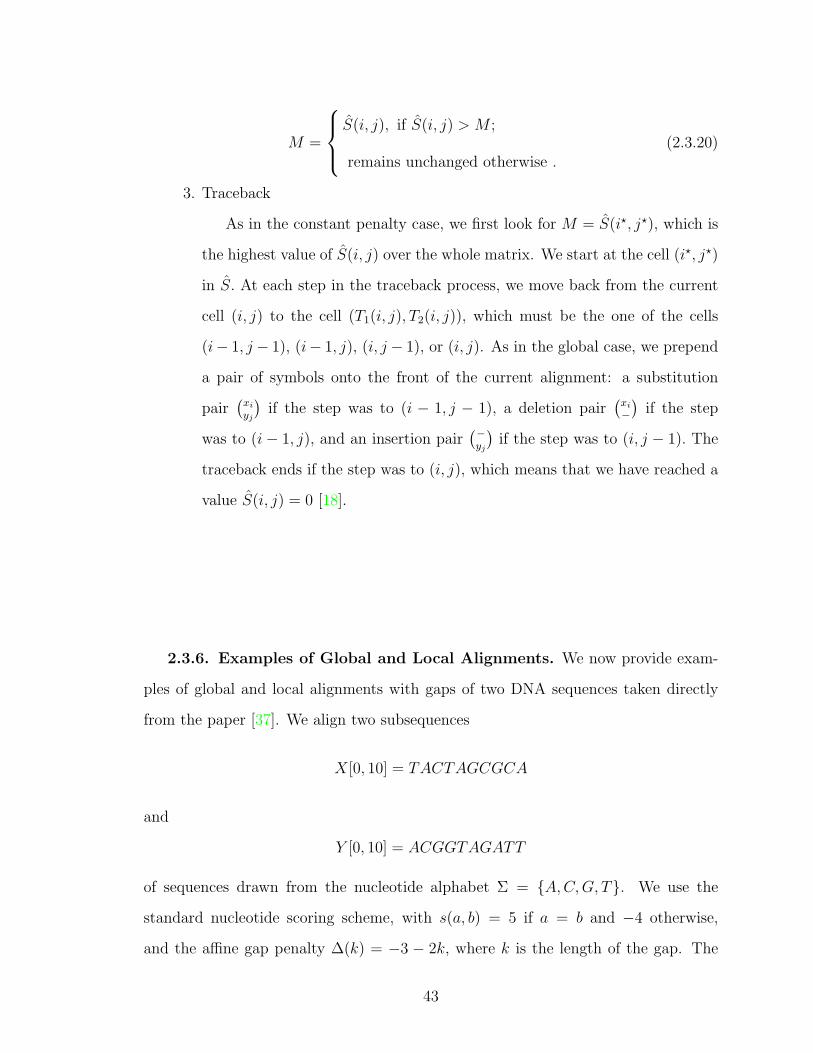
M =

S(i, j), if S(i, j) > M ;


3. Traceback

As in the constant penalty case, we first look for M = S(i?, j?), which is

the highest value of S(i, j) over the whole matrix. We start at the cell (i?, j?)

in S. At each step in the traceback process, we move back from the current

cell (i, j) to the cell (T1(i, j), T2(i, j)), which must be the one of the cells

(i− 1, j − 1), (i− 1, j), (i, j − 1), or (i, j). As in the global case, we prepend

a pair of symbols onto the front of the current alignment: a substitution

pair(xiyj


(xi−

)if the step

was to (i− 1, j), and an insertion pair(−yj

)if the step was to (i, j − 1). The

traceback ends if the step was to (i, j), which means that we have reached a

value S(i, j) = 0 [18].

2.3.6. Examples of Global and Local Alignments. We now provide exam-

ples of global and local alignments with gaps of two DNA sequences taken directly

from the paper [37]. We align two subsequences

X[0, 10] = TACTAGCGCA

and

Y [0, 10] = ACGGTAGATT

of sequences drawn from the nucleotide alphabet Σ = A,C,G, T. We use the

standard nucleotide scoring scheme, with s(a, b) = 5 if a = b and −4 otherwise,

and the affine gap penalty ∆(k) = −3 − 2k, where k is the length of the gap. The

43

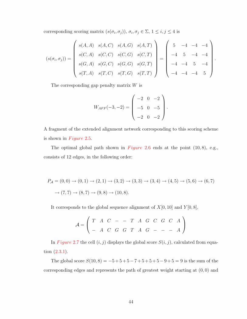
corresponding scoring matrix (s(σi, σj)), σi, σj ∈ Σ, 1 ≤ i, j ≤ 4 is

(s(σi, σj)) =

s(A,A) s(A,C) s(A,G) s(A, T )

s(C,A) s(C,C) s(C,G) s(C, T )

s(G,A) s(G,C) s(G,G) s(G, T )

s(T,A) s(T,C) s(T,G) s(T, T )

=

5 −4 −4 −4

−4 5 −4 −4

−4 −4 5 −4

−4 −4 −4 5

.

The corresponding gap penalty matrix W is

WAFF (−3,−2) =

−2 0 −2

−5 0 −5

−2 0 −2

.

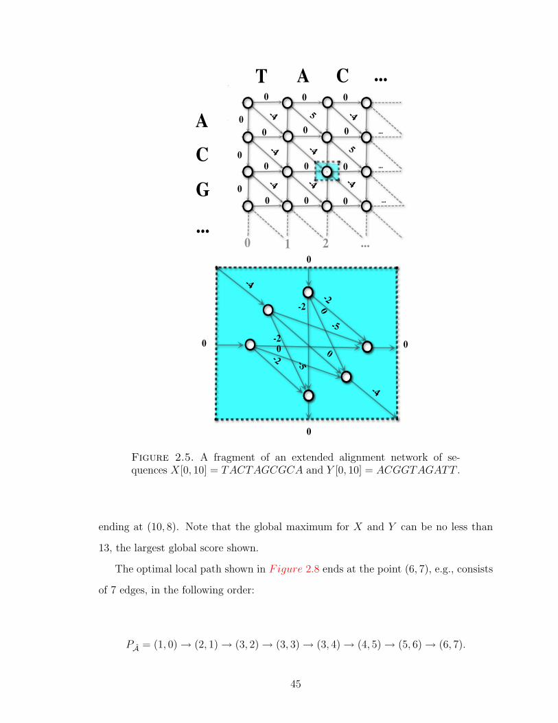
A fragment of the extended alignment network corresponding to this scoring scheme

is shown in Figure 2.5.

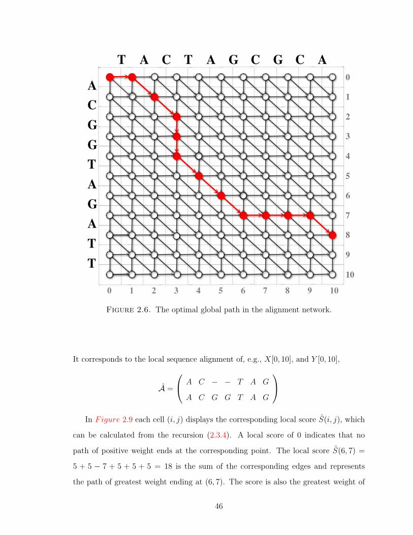
The optimal global path shown in Figure 2.6 ends at the point (10, 8), e.g.,

consists of 12 edges, in the following order:

PA = (0, 0)→ (0, 1)→ (2, 1)→ (3, 2)→ (3, 3)→ (3, 4)→ (4, 5)→ (5, 6)→ (6, 7)

→ (7, 7)→ (8, 7)→ (9, 8)→ (10, 8).

It corresponds to the global sequence alignment of X[0, 10] and Y [0, 8],

A =

T A C − − T A G C G C A

− A C G G T A G − − − A

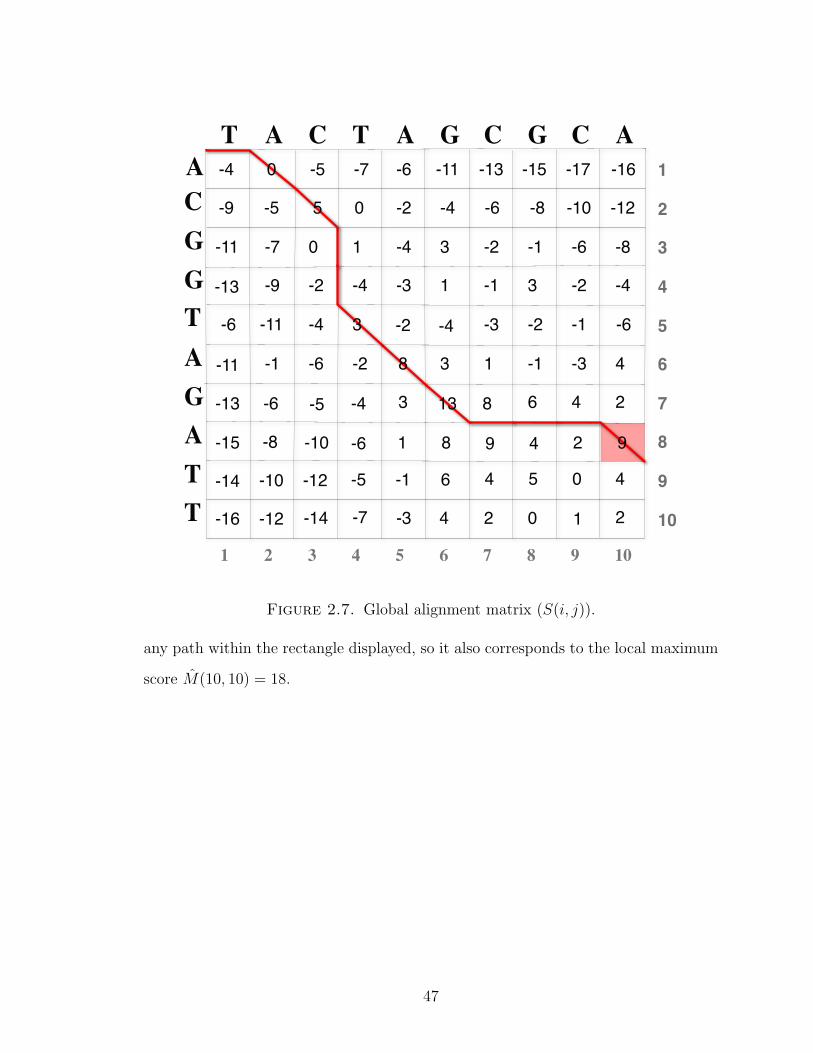
In Figure 2.7 the cell (i, j) displays the global score S(i, j), calculated from equa-

tion (2.3.1).

The global score S(10, 8) = −5 + 5 + 5−7 + 5 + 5 + 5−9 + 5 = 9 is the sum of the

corresponding edges and represents the path of greatest weight starting at (0, 0) and

44

0-2

-4

-4

-2

-5

-5

-2

0

0

0

0

-2

...

...

...

-4

-4

-4

-45

5

-4

...CA

G

CA

0 ...21...

0

0

0

0

0

0

0 0

0

0

0

00

T

-4

-400

0

0

Figure 2.5. A fragment of an extended alignment network of se-quences X[0, 10] = TACTAGCGCA and Y [0, 10] = ACGGTAGATT .

ending at (10, 8). Note that the global maximum for X and Y can be no less than

13, the largest global score shown.

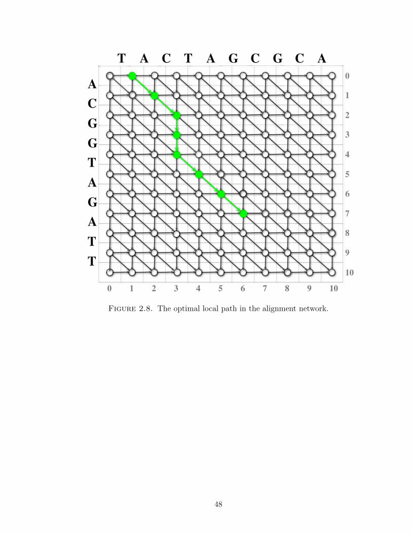
The optimal local path shown in Figure 2.8 ends at the point (6, 7), e.g., consists

of 7 edges, in the following order:

PA = (1, 0)→ (2, 1)→ (3, 2)→ (3, 3)→ (3, 4)→ (4, 5)→ (5, 6)→ (6, 7).

45

GATCA C

GATGGCA

0 654321

7

7

0

1

2

3

4

5

6

10

9

8

1098

ACG

TTA

T

Figure 2.6. The optimal global path in the alignment network.

It corresponds to the local sequence alignment of, e.g., X[0, 10], and Y [0, 10],

A =

A C − − T A G

A C G G T A G

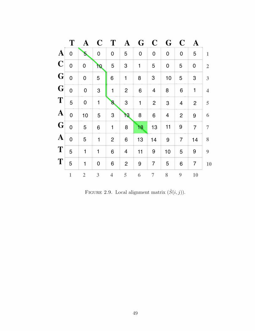
In Figure 2.9 each cell (i, j) displays the corresponding local score S(i, j), which

can be calculated from the recursion (2.3.4). A local score of 0 indicates that no

path of positive weight ends at the corresponding point. The local score S(6, 7) =

5 + 5 − 7 + 5 + 5 + 5 = 18 is the sum of the corresponding edges and represents

the path of greatest weight ending at (6, 7). The score is also the greatest weight of

46

GATCA C

GATGGCA

654321

7

7

1

2

3

4

5

6

10

9

8

1098

ACG

TTA

T

3-4-5-6 246-13

38-2-6-1 1 4-3-1-11

1-3-4-2-9 -1 -4-23-13

-4-23-4-11 -3 -6-1-2-6

3-410-7 -2 -8-6-1-11

-4-205-5 -6 -12-10-8-9

-11-6-7-5 -13 -16-17-15-4

4-3-7-14-12 2 210-16

8-6-10-8 9 4-15

6-1-5-12-10 4 45-14

0

13 8

1 2 9

0

Figure 2.7. Global alignment matrix (S(i, j)).

any path within the rectangle displayed, so it also corresponds to the local maximum

score M(10, 10) = 18.

47

GATCA C

GATGGCA

0 654321

7

7

0

1

2

3

4

5

6

10

9

8

1098

ACG

TTA

T

Figure 2.8. The optimal local path in the alignment network.

48

GATCA C

GATGGCA

654321

7

7

1

2

3

4

5

6

10

9

8

1098

ACG

TTA

T

8165 79110

8133510 6 9240

62130 4 1680

13810 2 2435

81650 3 35100

135100 5 0500

0500 0 5000

92601 7 7655

1315 14 90

461 9 105

18 13

6 7 14

5

2

1 11 5 9

Figure 2.9. Local alignment matrix (S(i, j)).

49

Chapter 3

Statistics of Local Sequence Alignment

“The patient is more alive then dead”

N. Nosov from ”The Adventures of Neznaika and His Friends” [48]

3.1. Hypothesis Testing

Suppose we have to make a binary decision based on some evidence, where the

term binary indicates two mutually excluding options. A theory that can help us

with this task is called hypothesis testing. A formal model for statistical hypothesis

testing was proposed by J. Neyman and E. S. Pearson in the late 1920s and 1930s. In

hypothesis testing, the states of nature are partitioned into two sets or hypotheses.

The goal of hypothesis testing is to decide which hypothesis is correct, i.e., which

hypothesis contains the true state of nature. We need to distinguish between two

hypothesis, so we call them the null hypothesis H0 and the alternative hypothesis

H1. Traditionally, the null hypothesis is the one that we accept by default even if the

evidences for both H0 and H1 are equivocal and H1 is the hypothesis that requires

compelling evidence in order to be accepted. Generally, H0 is a mathematical model

of randomness with respect to a particular set of observations. It gives a chance

50

its privileged status in statistical theory. The purpose of most statistical tests is

to determine whether the observed data can be explained by the null hypothesis.

For this purpose P -values are used. In the case of database retrieval, E-values are

used instead of P -values. The P -value is the probability of observing an effect as

strong or stronger than you observed, given the null hypothesis, thus it answers the

question “How likely is this effect to occur by chance?”. The lower the P -value, the

less likely the result, assuming the null hypothesis, the more significant the result,

in the sense of statistical significance. In the case of database retrieval, i.e. when

we list/retrieve the highest scoring sequences that are supposedly homologous with

our query sequence, a P -value by itself is not informative enough. For example, let

our null hypothesis be that our alignment comes from the random model R and the

alternative hypothesis that our alignment is real, coming from the match model M .

Consider a score that corresponds to a P -value 10−4. On the face of it, this seems a

very unlikely event. Roughly speaking, we would expect to see an alignment at least

this good only once in every 10, 000 alignments. Now, if our database has a large size

(say, 100, 000), we would still expect to see quite a few chance alignments that are

as good as the one we consider. Thus, the E-value — the expected number of times

that we would see a result at least as good as the one we have in a random database

of the given size — is a better way to judge whether we have compelling evidence to

accept our alternative hypothesis. To assess whether a given alignment constitutes

evidence for homology, it helps to know how strong an alignment can be expected from

chance alone. In this context, “chance” can mean the comparison of sequences that

are generated randomly based upon a DNA or protein sequence model. In sequence

similarity search, homology relationship is inferred based on P -values or its equivalent

E-values. These values help to decide on two hypotheses: H0 - an alignment score

was obtained by chance, meaning that sequences are not homologous, and H1 - the

score is significant and sequences are homologous.

51

If a local alignment has score x, the P -value gives the probability that a local

alignment having score x or greater is found by chance. The smaller the P -value,

the greater the belief that the aligned sequences are homologous. Accordingly, two

sequences are reported to be homologous if they are aligned extremely well, which

serves as a compelling evidence.

The BLAST program (Basic Local Alignment Search Tool [4]) is the most widely

used tool for homology search in DNA and protein database. It finds regions of local

similarity between a query sequence and each database sequence. It also calculates the

statistical significance of matches. It has been used by numerous biologists to reveal

functional and evolutionary relationships between sequences and identify members of

gene families. A P -value of 10−5 is often used as a cutoff for BLAST database search.

It means that with a collection of random query sequences, only once in a hundred

thousand of instances would an alignment with that score or greater occur by chance.

52

3.2. Random Variables and Random Processes

In order to understand the rigorous statistical theory implemented in BLAST we

first introduce more facts from probability theory. Proofs and further details on this

topic can be found in [20], [23], [43].

Consider a probability space Ω,F ,P defined in Chapter 2. Sometimes we are

more interested in the consequence of the random outcome of an experiment then in

the experiment itself. When we assign real values to such consequences we can think

of them as functions. Such functions are called random variables.

Definition 17. A random variable is a function X : Ω → R with the property that

ω ∈ Ω : X(ω) ≤ x ∈ F for each x ∈ R. Such a function is said to be F -measurable.

The value taken by a random variable is subject to chance. We shall denote

random variables by upper-case letters X, Y, and Z etc., and numerical values of a

random variable by lowercase letters x, y, and z, etc. For a random variable X and

a real number x, the expression X ≤ x denotes the event that X has a value less

then or equal to x. The probability that the event occurs is denoted by P[X ≤ x].

Definition 18. The distribution function of a random variable X is the function

FX : R→ [0, 1] given by FX(x) = P[X ≤ x].

There are two important classes of random variables: discrete and continuous.

Definition 19. The random variable X is called discrete if it takes values in some

countable subset x1, x2, . . ., of R. The discrete random variable X has probability

mass function f : R → [0, 1] given by f(x) = P[X = x]. The distribution and mass

functions are related by

FX(x) =∑i:xi≤x

f(xi).

53

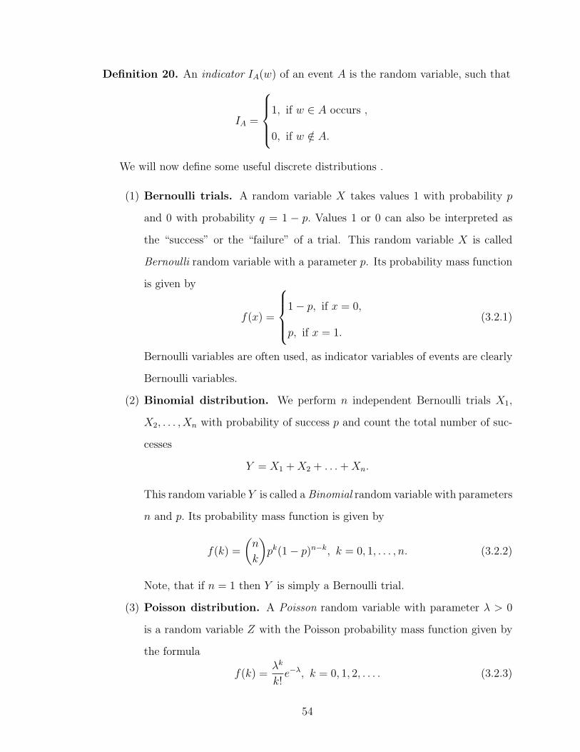
Definition 20. An indicator IA(w) of an event A is the random variable, such that

IA =

1, if w ∈ A occurs ,

0, if w /∈ A.

We will now define some useful discrete distributions .

(1) Bernoulli trials. A random variable X takes values 1 with probability p

and 0 with probability q = 1 − p. Values 1 or 0 can also be interpreted as

the “success” or the “failure” of a trial. This random variable X is called

Bernoulli random variable with a parameter p. Its probability mass function

is given by

f(x) =

1− p, if x = 0,

p, if x = 1.

(3.2.1)

Bernoulli variables are often used, as indicator variables of events are clearly

Bernoulli variables.

(2) Binomial distribution. We perform n independent Bernoulli trials X1,

X2, . . . , Xn with probability of success p and count the total number of suc-

cesses

Y = X1 +X2 + . . .+Xn.

This random variable Y is called a Binomial random variable with parameters

n and p. Its probability mass function is given by

f(k) =

(n

k

)pk(1− p)n−k, k = 0, 1, . . . , n. (3.2.2)

Note, that if n = 1 then Y is simply a Bernoulli trial.

(3) Poisson distribution. A Poisson random variable with parameter λ > 0

is a random variable Z with the Poisson probability mass function given by

the formula

f(k) =λk

k!e−λ, k = 0, 1, 2, . . . . (3.2.3)

54

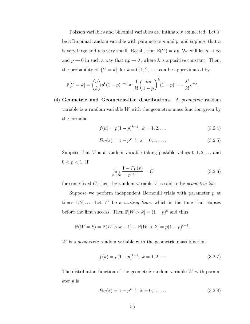
Poisson variables and binomial variables are intimately connected. Let Y

be a Binomial random variable with parameters n and p, and suppose that n

is very large and p is very small. Recall, that E(Y ) = np. We will let n→∞

and p→ 0 in such a way that np→ λ, where λ is a positive constant. Then,

the probability of Y = k for k = 0, 1, 2, . . . . can be approximated by

P[Y = k] =

(n

k

)pk(1− p)n−k ≈ 1

k!

(np

1− p

)k(1− p)n → λk

k!e−λ.

(4) Geometric and Geometric-like distributions. A geometric random

variable is a random variable W with the geometric mass function given by

the formula

f(k) = p(1− p)k−1, k = 1, 2, . . . (3.2.4)

FW (x) = 1− px+1, x = 0, 1, . . . . (3.2.5)

Suppose that V is a random variable taking possible values 0, 1, 2, . . . and

0 < p < 1. If

limv→∞

1− FV (v)

pv+1= C (3.2.6)

for some fixed C, then the random variable V is said to be geometric-like.

Suppose we perform independent Bernoulli trials with parameter p at

times 1, 2, . . . . Let W be a waiting time, which is the time that elapses

before the first success. Then P[W > k] = (1− p)k and thus

P(W = k) = P(W > k − 1)− P(W > k) = p(1− p)k−1.

W is a geometric random variable with the geometric mass function

f(k) = p(1− p)k−1, k = 1, 2, . . . (3.2.7)

The distribution function of the geometric random variable W with param-

eter p is

FW (x) = 1− px+1, x = 0, 1, . . . . (3.2.8)

55

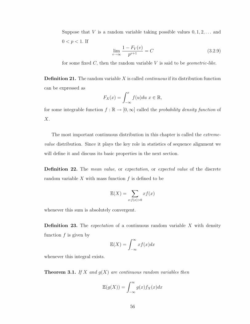
Suppose that V is a random variable taking possible values 0, 1, 2, . . . and

0 < p < 1. If

limv→∞

1− FV (v)

pv+1= C (3.2.9)

for some fixed C, then the random variable V is said to be geometric-like.

Definition 21. The random variableX is called continuous if its distribution function

can be expressed as

FX(x) =

∫ x

−∞f(u)du x ∈ R,

for some integrable function f : R→ [0,∞] called the probability density function of

X.

The most important continuous distribution in this chapter is called the extreme-

value distribution. Since it plays the key role in statistics of sequence alignment we

will define it and discuss its basic properties in the next section.

Definition 22. The mean value, or expectation, or expected value of the discrete

random variable X with mass function f is defined to be

E(X) =∑

x:f(x)>0

xf(x)

whenever this sum is absolutely convergent.

Definition 23. The expectation of a continuous random variable X with density

function f is given by

E(X) =

∫ ∞−∞

xf(x)dx

whenever this integral exists.

Theorem 3.1. If X and g(X) are continuous random variables then

E(g(X)) =

∫ ∞−∞

g(x)fX(x)dx

56

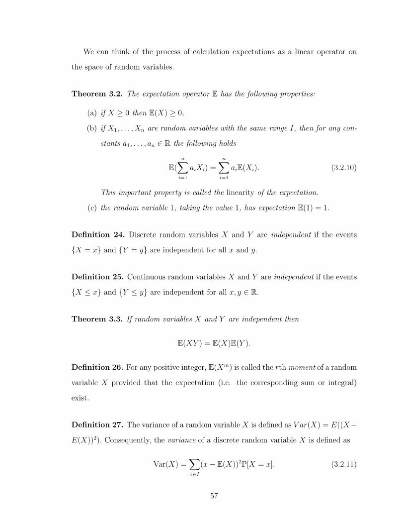
We can think of the process of calculation expectations as a linear operator on

the space of random variables.

Theorem 3.2. The expectation operator E has the following properties:

(a) if X ≥ 0 then E(X) ≥ 0,

(b) if X1, . . . , Xn are random variables with the same range I, then for any con-

stants a1, . . . , an ∈ R the following holds

E(n∑i=1

aiXi) =n∑i=1

aiE(Xi). (3.2.10)

This important property is called the linearity of the expectation.

(c) the random variable 1, taking the value 1, has expectation E(1) = 1.

Definition 24. Discrete random variables X and Y are independent if the events

X = x and Y = y are independent for all x and y.

Definition 25. Continuous random variables X and Y are independent if the events

X ≤ x and Y ≤ y are independent for all x, y ∈ R.

Theorem 3.3. If random variables X and Y are independent then

E(XY ) = E(X)E(Y ).

Definition 26. For any positive integer, E(Xm) is called the rth moment of a random

variable X provided that the expectation (i.e. the corresponding sum or integral)

exist.

Definition 27. The variance of a random variable X is defined as V ar(X) = E((X−

E(X))2). Consequently, the variance of a discrete random variable X is defined as

Var(X) =∑x∈I

(x− E(X))2P[X = x], (3.2.11)

57

where I is the range of X. Similarly, the variance of a continuous random variable Y

is defined by

Var(Y ) =

∫ ∞−∞

(y − E(Y ))2fY (y)dy. (3.2.12)

Definition 28. The moment-generating function (MGF) of a random variable X is

written MX(t) and defined as

MX(t) = E(etX).

For a discrete random variable X having range I,

MX(t) =∑x∈I

etxP[X = x].

For a continuous random variable Y having density function fY ,

MY (t) =

∫ ∞−∞

etyfY (y)dy.

Any moments of a random variable can be expressed as an appropriate differen-

tiation of its MGF. In particular, for any random variable X,

E(X) =

(dMX(t)

dt

)t=0

and

V ar(X) =

(d2MX(t)

dt2

)t=0

− E2(X) =

(d2 lnMX(t)

dt2

)t=0

.

The following property of MGFs plays a critical role in the scoring matrix and

local alignment statistics.

Theorem 3.4. Let X be a discrete random variable with MX(t) converging for all t

in (−∞,∞). Suppose that X takes at least one negative value and one positive value

with nonzero probability and that E(X) 6= 0. Then there exists a unique nonzero value

θ such that MX(θ) = 1.

58

Definition 29. A random process is a family of random variables X(t), t ∈ T

indexed by the parameter t, where t varies over an index set T. The index set T

is calles the parameter set of the random process. The values assumed by X(t) are

called states, and the set of all possible values forms the state space of the random

process.

We will define two important random processes: a random walk and a renewal

process. In both processes the parameter set and the state space are discrete sets.

Definition 30. Suppose that X1, X2, . . . are independent random variables, each

taking values xi ∈ −n,−n+1, . . . ,m−1,m, for i ≥ 1 and n,m ∈ N with respective

probabilities

p−n, p−n+1, . . . , p−1, p0, p1, . . . , pm−1, pm,

and consider the sum Sn =∑n

i=1 Xi, then the sequence S = Si : i ≥ 0 where S0 = 0

is called a generalised random walk in one dimension starting at the origin. When

X1, X2, . . . take values 1 with probability p, and −1 otherwise, then the sequence

S = Si : i ≥ 0 where S0 = 0 is called a simple random walk in one dimension

starting at the origin.

Definition 31. A renewal process N = N(t) : t ≥ 0 is a process such that

N(t) = maxn : Tn ≤ t

where T0 = 0, Tn = X1+X2+. . .+Xn for n ≥ 1, and Xi is a sequence of independent

identically distributed non-negative random variables.

We can think of a renewal process N(t) as representing the number of occurrences

of some event in the time interval [0, t]; the event in question might be the arrival of

a person or particle, or a failure of a light bulb. We shall speak of Tn as the time of

nth arrival and Xn as the nth interarrival time.

59

Consider an infinite sequence of repeated trials with possible outcomes Xi, i =

1, 2 . . . Let B be an event defined by an attribute of the finite sequences of possible

outcomes Xi. We say that B occurs at the ith trial if the outcomes X1, X2, . . . , Xi

have the attribute. H is a recurrent event if, under the condition the H occurs at

the ith trial, we have that the probability that X1, X2, . . . , Xi+k have the attribute

is equal to the product of the probabilities that X1, X2, . . . , Xi have the attribute

and Xi+1, Xi+2, . . . , Xi+k have the attribute. For instance, the event that a success

followed by failure is a recurrent event in a sequence of Bernoulli trials.

For a recurrent event H, we are interested in the following two probabilistic dis-

tributions:

uj = P[H occurs at the ith trial ], i = 1, 2, . . . ,

fi = P[H occurs for the first time at the ith trial ], i = 1, 2, . . . ,

Then the mean waiting time between two successive occurrences of H is

E(H) =∑i

ifi. (3.2.13)

Theorem 3.5. If E(H) is finite, then un → 1E(H)

as n→∞.

Define the indicator variable Ij for each j as

Ij =

1, if H occurs at the jth trial,

0, if it does not.

Then, the sum

Xk = I1 + I2 + . . .+ Ik

60

denotes the number of occurrences of H in the first k trials. By the linearity property

of the expectation, we have

E(Xk) = E(I1) + E(I2) + . . .+ E(Ik) = u1 + u2 + . . .+ uk.

If E(H) is finite, by Theorem 3.5, we have

E(XN) ≈N

E(H). (3.2.14)

Definition 32. The Renewal Equation is a convolution equation relating bounded

sequences νii≥0 and bii≥0 of real numbers:

νn = bn +n∑k=1

fkνn−k, n = 0, 1, . . . . (3.2.15)

where fkk≥1 is the interarrival time distribution for the renewal process.

The following theorem provides conditions under which the sequence νn defined

through convolution equation converges as n goes to infinity.

Theorem 3.6. If∑

i bi = B <∞,∑

i fi = 1, and ξ =∑

i ifi <∞, and the greatest

common divisor of indicies i such that fi 6= 0 is 1, then

νn →B

ξ

as n→∞.

61

3.3. Ungapped Local Alignment Scores Statistics

3.3.1. Ungapped local alignment scores. To study the distribution of op-

timal local ungapped alignment scores, we use the random model R, introduced in

a previous chapter. Recall, that within this model we assume that the two aligned

sequences are made up of residues i that are drawn independently with different prob-

abilities pi. These probabilities define the background frequency distribution of the

aligned sequences. We denote the score for aligning residues i and j by sij. If at

least one score sij is positive and the expected score for aligning two randomly chosen

residues is negative, i.e.

E(sij) =∑i,j

pipjsij < 0, (3.3.1)

the optimal local ungapped alignment scores approach an extreme value distribu-

tion when sequences are sufficiently long. Moreover, simple formulas are available for

the corresponding parameters λ and µ [31], [30], [16].

The scale parameter λ is the unique positive number satisfying the following equa-

tion

∑i,j

pipjeλsij = 1. (3.3.2)

Thus, by (3.3.2), λ depends on the scoring matrix (sij) and the background fre-

quencies (pi). It converts pairwise match scores to a probabilistic distribution pipjeλsij .

The location parameter µ is given by

µ =log(Kmn)

λ, (3.3.3)

where m and n are the lengths of aligned sequences and K < 1. K is considered

as a space correcting factor because optimal local alignments cannot locate in all mn

possible sites. It is analytically given by a geometrically convergent series, depending

only on the (pi) and (sij)

62

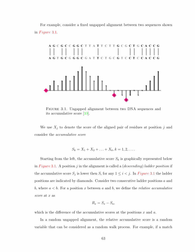
For example, consider a fixed ungapped alignment between two sequences shown

in Figure 3.1.

G TCTTATC TGGCCGC CACGTCGCGTA GC

G GTCTTAC GGGGCGT CACCTCCTGCA GC

Figure 3.1. Ungapped alignment between two DNA sequences andits accumulative score [10].

We use Xj to denote the score of the aligned pair of residues at position j and

consider the accumulative score

Sk = X1 +X2 + . . .+Xk, k = 1, 2, . . . .

Starting from the left, the accumulative score Sk is graphically represented below

in Figure 3.1. A position j in the alignment is called a (descending) ladder position if

the accumulative score Sj is lower then Si for any 1 ≤ i < j. In Figure 3.1 the ladder

positions are indicated by diamonds. Consider two consecutive ladder positions a and

b, where a < b. For a position x between a and b, we define the relative accumulative

score at x as

Rx = Sx − Sa,

which is the difference of the accumulative scores at the positions x and a.

In a random ungapped alignment, the relative accumulative score is a random

variable that can be considered as a random walk process. For example, if a match

63

score is s and it occurs with probability p, then Rx can be considered as the distance

from 0 in a random walk that moves right with probability p or left with probability

1 − p and stops at −1 on the state set −1, 0, 1, . . . . The state −1 is called the

absorbing state, which is the state the walk once reaches and never leaves.

The local alignment between a ladder position where the highest relative accumu-

lative score attains before the next ladder position gives a maximal scoring segment

in the alignment. In 1992 Karlin and Dembo published the paper [31], where they

derived the explicit limit distribution of maximal scoring segments. Their method

was based on the estimation of the following two quantities:

(i) The probability distribution of the maximum value that the corresponding

random walk ever achieves before stopping at the absorbing state, and

(ii) The mean number of steps before the corresponding random walk first reaches

the absorbing state.

In sections 3.3.2, 3.3.3, and 3.3.4 we will provide basic results from the paper [31]

with proofs.

3.3.2. Maximum Segment Scores. When two sequences are aligned, scores

are taken from a substitution matrix, for example, BLOSUM62. Because such ma-

trices are integer valued, the accumulative score performes a complicated random

walk.

Consider a random walk that starts at 0 and whose possible step sizes are

−d,−d+ 1, . . . ,−1, 0, 1, . . . , c− 1, c

with respective probabilities

p−d, p−d+1, . . . , p−1, p0, p1, . . . , pc−1, pc

such that

(i) p−d > 0, pc > 0, and pi ≥ 0,−d < i < c, and

64

(ii) the mean step size∑c

j=−d jpj < 0.

We denote the score of the aligned pair at the ith position by Xi. Clearly, Xis

are independent identically distributed (i.i.d.) random variables. Consider a random

variable X with the same distribution as Xis. The moment generating function of X

is

E(eθX) =c∑

j=−d

pjejθ.

We consider the accumulative scores:

S0 = 0,

Sj =

j∑i=1

Xi, j = 1, 2, . . . ,

and partition the walk into non-negative excursions between the successive de-

scending ladder positions in the path as shown in Figure 3.2:

K0 = 0,

Ki = mink|k ≥ Ki−1 + 1, Sk < SKi−1, i = 1, 2, . . . . (3.3.4)

Because the mean step size is negative, the Ki −Ki−1 are positive integer-valued

i.i.d. random variables. Define Qi to be the maximal score attained during the ith

excursion between Ki−1 and Ki, i.e.

Qi = maxKi−1≤k<K1

(Sk − SKi−1), i = 1, 2, . . . . (3.3.5)

The Qis are non-negative i.i.d. random variables. We will estimate P[Q1 ≤ x] and

E(K1).

Define

t+ = mink|Sk > 0, Si ≤ 0, i = 1, 2, . . . , k − 1, (3.3.6)

65

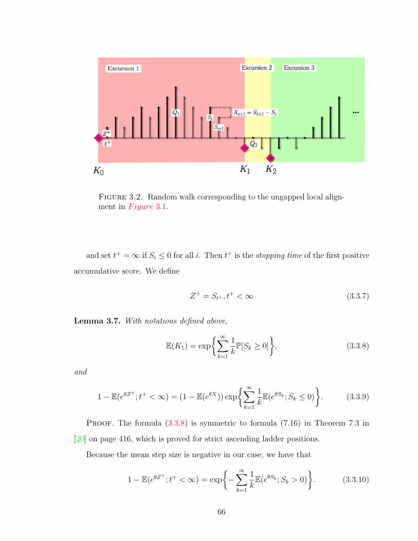
Figure 3.2. Random walk corresponding to the ungapped local align-ment in Figure 3.1.

and set t+ =∞ if Si ≤ 0 for all i. Then t+ is the stopping time of the first positive

accumulative score. We define

Z+ = St+ , t+ <∞ (3.3.7)

Lemma 3.7. With notations defined above,

E(K1) = exp

∞∑k=1

1

kP[Sk ≥ 0]

, (3.3.8)

and

1− E(eθZ+

; t+ <∞) = (1− E(eθX)) exp

∞∑k=1

1

kE(eθSk ;Sk ≤ 0)

. (3.3.9)

Proof. The formula (3.3.8) is symmetric to formula (7.16) in Theorem 7.3 in

[20] on page 416, which is proved for strict ascending ladder positions.

Because the mean step size is negative in our case, we have that

1− E(eθZ+

; t+ <∞) = exp

−∞∑k=1

1

kE(eθSk ;Sk > 0)

. (3.3.10)

66

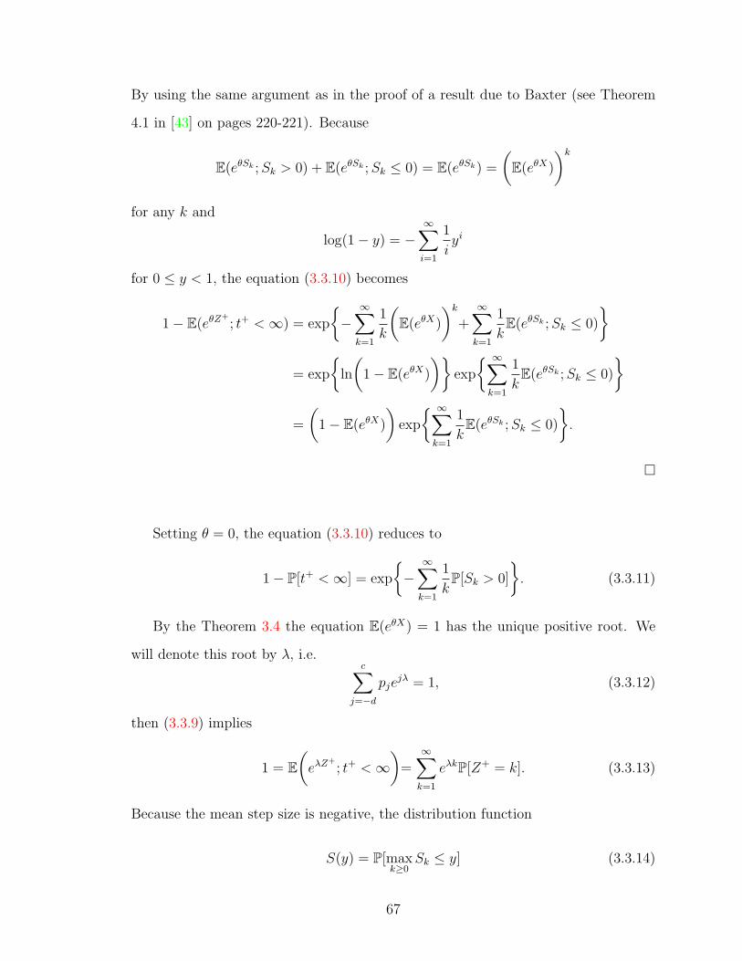
By using the same argument as in the proof of a result due to Baxter (see Theorem

4.1 in [43] on pages 220-221). Because

E(eθSk ;Sk > 0) + E(eθSk ;Sk ≤ 0) = E(eθSk) =

(E(eθX)

)kfor any k and

log(1− y) = −∞∑i=1

1

iyi

for 0 ≤ y < 1, the equation (3.3.10) becomes

1− E(eθZ+

; t+ <∞) = exp

−∞∑k=1

1

k

(E(eθX)

)k+∞∑k=1

1

kE(eθSk ;Sk ≤ 0)

= exp

ln

(1− E(eθX)

)exp

∞∑k=1

1

kE(eθSk ;Sk ≤ 0)

=

(1− E(eθX)

)exp

∞∑k=1

1

kE(eθSk ;Sk ≤ 0)

.

Setting θ = 0, the equation (3.3.10) reduces to

1− P[t+ <∞] = exp

−∞∑k=1

1

kP[Sk > 0]

. (3.3.11)

By the Theorem 3.4 the equation E(eθX) = 1 has the unique positive root. We

will denote this root by λ, i.e.c∑

j=−d

pjejλ = 1, (3.3.12)

then (3.3.9) implies

1 = E(eλZ

+

; t+ <∞)

=∞∑k=1

eλkP[Z+ = k]. (3.3.13)

Because the mean step size is negative, the distribution function

S(y) = P[maxk≥0

Sk ≤ y] (3.3.14)

67

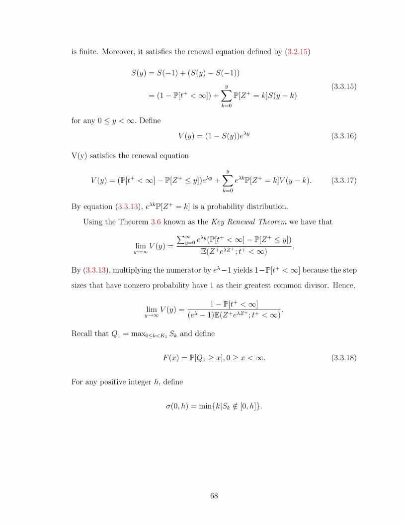
is finite. Moreover, it satisfies the renewal equation defined by (3.2.15)

S(y) = S(−1) + (S(y)− S(−1))

= (1− P[t+ <∞]) +

y∑k=0

P[Z+ = k]S(y − k)(3.3.15)

for any 0 ≤ y <∞. Define

V (y) = (1− S(y))eλy (3.3.16)

V(y) satisfies the renewal equation

V (y) = (P[t+ <∞]− P[Z+ ≤ y])eλy +

y∑k=0

eλkP[Z+ = k]V (y − k). (3.3.17)

By equation (3.3.13), eλkP[Z+ = k] is a probability distribution.

Using the Theorem 3.6 known as the Key Renewal Theorem we have that

limy→∞

V (y) =

∑∞y=0 e

λy(P[t+ <∞]− P[Z+ ≤ y])

E(Z+eλZ+ ; t+ <∞).

By (3.3.13), multiplying the numerator by eλ−1 yields 1−P[t+ <∞] because the step

sizes that have nonzero probability have 1 as their greatest common divisor. Hence,

limy→∞

V (y) =1− P[t+ <∞]

(eλ − 1)E(Z+eλZ+ ; t+ <∞).

Recall that Q1 = max0≤k<K1 Sk and define

F (x) = P[Q1 ≥ x], 0 ≥ x <∞. (3.3.18)

For any positive integer h, define

σ(0, h) = mink|Sk /∈ [0, h].

68

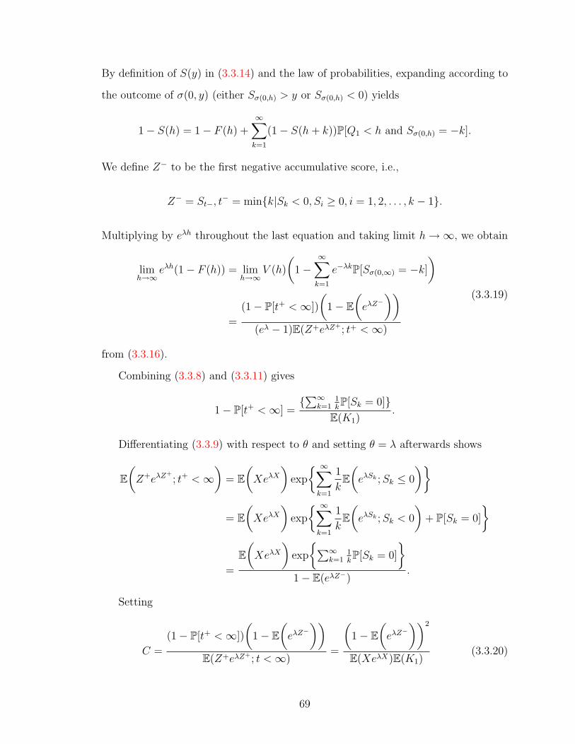
By definition of S(y) in (3.3.14) and the law of probabilities, expanding according to

the outcome of σ(0, y) (either Sσ(0,h) > y or Sσ(0,h) < 0) yields

1− S(h) = 1− F (h) +∞∑k=1

(1− S(h+ k))P[Q1 < h and Sσ(0,h) = −k].

We define Z− to be the first negative accumulative score, i.e.,

Z− = St−, t− = mink|Sk < 0, Si ≥ 0, i = 1, 2, . . . , k − 1.

Multiplying by eλh throughout the last equation and taking limit h→∞, we obtain

limh→∞

eλh(1− F (h)) = limh→∞

V (h)

(1−

∞∑k=1

e−λkP[Sσ(0,∞) = −k]

)

=

(1− P[t+ <∞])

(1− E

(eλZ

−))

(eλ − 1)E(Z+eλZ+ ; t+ <∞)

(3.3.19)

from (3.3.16).

Combining (3.3.8) and (3.3.11) gives

1− P[t+ <∞] =∑∞

k=11kP[Sk = 0]

E(K1).

Differentiating (3.3.9) with respect to θ and setting θ = λ afterwards shows

E(Z+eλZ

+

; t+ <∞)

= E(XeλX

)exp

∞∑k=1

1

kE(eλSk ;Sk ≤ 0

)

= E(XeλX

)exp

∞∑k=1

1

kE(eλSk ;Sk < 0

)+ P[Sk = 0]

=

E(XeλX

)exp

∑∞k=1

1kP[Sk = 0]

1− E(eλZ−)

.

Setting

C =

(1− P[t+ <∞])

(1− E

(eλZ

−))

E(Z+eλZ+ ; t <∞)=

(1− E

(eλZ

−))2

E(XeλX)E(K1)(3.3.20)

69

we have proved the folowing theorem:

Theorem 3.8. Assume the step sizes that have nonzero probability do not have non-

trivial common divisors. With notations defined above,

limh→∞

(1− F (h))eλh =C

eλ − 1, (3.3.21)

where λ is defined in (3.3.12).

Consider a random ungapped alignment A. Q1 defined for the random walk cor-

responding to A is equal to a maximal seqment score of it. Hence, 1− F (s) denotes

the probability of a maximal segment having score s or more in A. By Theorem 3.8,

the maximal segment scores have a geometric-like distribution as defined in (3.2.9).

3.3.3. E-value and P -value estimation. Here, we continue the derivation of

formulas for the estimation of the tail distribution of maximal segment scores in

ungapped alignment.

Consider the successive excursions with associated local maxima Qk defined in

(3.3.5). Define

M(Km) = maxk≤m

Qk (3.3.22)

and

C ′ =C

eλ − 1. (3.3.23)

Lemma 3.9. With notation defined above,

lim infm→∞

P[M(Km) ≤ lnm

λ+ y

]≥ exp

−C ′eλ−λy

,

lim supm→∞

P[M(Km) ≤ lnm

λ+ y

]≤ exp

−C ′e−λy

.

Proof. Because Q1, Q2, . . . , Qm are i.i.d. random variables,

P[M(Km) ≤ x] = (F (x))m. (3.3.24)

70

for any 0 < x ≤ ∞, where F (x) is the distribution function of Q1 and is defined in

(3.3.18). For any real number x <∞,

1− F (dxe) ≤ 1− F (x) ≤ 1− F (bxc).

Hence,

lim infx→∞

(1− F (x))eλx ≥ lim infx→∞

(1− F (dxe))eλdxe =C

eλ − 1= C ′

On the other hand, because lim supx→∞ x− bxc = 1,

lim supx→∞

(1− F (x))eλx ≤ limx→∞

(1− F (bxc))ebxceλx−bxc ≤ C

eλ − 1eλ = C ′eλ.

Replacing x by ln(m)/λ+ y, (3.3.24) becomes

P[M(Km) ≤ ln(m)/λ+ y] = (F (ln(m)/λ+ y))m =1

exp−m ln(F (ln(m)/λ+ y)).

Using

limz→1

ln z

z − 1= 1,

we obtain

lim supm→∞

P[M(Km) ≤ ln(m)/λ+ y] = lim supm→∞

1

exp−m ln(F (ln(m)/λ+ y))

=1

lim infm→∞ expm(1− F (ln(m)/λ+ y))

≤ 1

lim infm→∞ expmC ′e−(ln(m)+λy)

= exp

−C ′e−λy

.

71

Similarly,

lim infm→∞

P[M(Km) ≤ ln(m)/λ+ y] = lim infm→∞

1

exp−m ln(F (ln(m)/λ+ y))

=1

lim supm→∞ expm(1− F (ln(m)/λ+ y))

≥ 1

lim supm→∞ expmC ′eλe−(ln(m)+λy)

= exp

−C ′eλe−λy

.

Hence, the lemma is proved.

Now consider the accumulative score walk W corresponding to an ungapped align-

ment of length n. Let

A = E(K1), (3.3.25)

which is the mean distance between two successive ladder positions in the walk. Then

the mean number of ladder positions is approximately nA

when n is large. Ignoring

edge effects, we derive the following asymptotic bounds from Lemma 3.9 by setting

y = y′ + lnAλ

and m = nA

:

exp

−C

′eλ

Ae−λy′

≤ P

[M(n) ≤ lnn

λ+ y′

]≤ exp

−C

′

Ae−λy

′. (3.3.26)

Set

K =C ′

A. (3.3.27)

Replacing y′ by (ln(K) + s)/λ, inequality (3.3.26) becomes

exp

−eλ−s

≤ P[M(n) ≤ ln(Kn) + s/λ] ≤ exp−e−s,

or equivalently

exp

−eλ−s

≤ P[λM(n)− ln(Kn) ≤ s] ≤ exp−e−s. (3.3.28)

72

In the BLAST theory, the expression

Y (n) = λM(n)− ln(Kn)

is called the normalized score of the alignment. Hence, the P -value corresponding

to an observed value s of the normalized score is

P -value ≈ 1− exp−e−s. (3.3.29)

3.3.4. The Number of High-Scoring Segments. By Theorem 3.8 and equa-

tion (3.3.23), the probability that any maximal-scoring segment has score s or more

is approximately C ′e−λs. By (3.3.25), to a close approximation there are NA

maximal

scoring segments in a fixed alignment of N columns as discussed in the previous sec-

tion. Hence, the expected number of the maximal-scoring segments with score s or

more is approximately

NC ′

Ae−λs = NKe−λs, (3.3.30)

where K is defined in (3.3.27).

3.3.5. Karlin-Altschul Sum Statistic. When two sequences are aligned, in-

sertions and deletions can break a long alignment into several parts. In this case, it

is useful to consider the scores of the multiple highest-scoring segments.

Denote the r disjoint highest segment scores as

M (1),M (2), . . . ,M (r)

in an alignment with n columns. We consider the normalized scores

S(i) = λM (i) − ln(Kn), i = 1, 2, . . . , r. (3.3.31)

73

Karlin and Altschul in 1993 [30] showed that the limiting joint density fS(x1, x2, . . . , xr)

of S = (S(1), S(2), . . . , S(r)) is

S(x1, x2, . . . , xr) = exp

(−e−xr −

r∑k=1

xk

)(3.3.32)

in the domain x1 ≥ x2 ≥ . . . ≥ xr.

Assessing multiple highest-scoring segments is more involved that it might first

appear. Suppose, for example, comparison X reports two highest scores 108 and 88,

whereas comparison Y reports 99 and 90. One can say that Y is not better that

X, because its high score is lower than of X. But neither is X considered better,

because the second high score is lower than that of Y . The natural way to rank all

possible results is to consider the sum of the normalized scores of the r highest scoring

segments

Sn,r = S(1) + S(2) + . . .+ S(r) (3.3.33)

as suggested by Karlin and Altschul. This sum is now called the Karlin− Altschul

sum statistic.

Theorem 3.10. The limiting density function of Karlin-Altschul sum Sn,r is

fn,r(x) =e−x

r!(r − 2)!

∫ ∞0

yr−2 exp(−e(y−x)/r)dy. (3.3.34)

Integration fn,r(x) from t to ∞ gives the tail probability that Sn,r ≥ r. This

resulting double integral can be easily calculated numerically. Asymptotically, the

tail probability is well approximated by the formula

P[Sn,r ≥ r] =e−ttr−1

r!(r − 1)!. (3.3.35)

especially when t > r(r − 1). This is the formula used in the BLAST program for

calculation P -value when multiple highest-scoring segments are reported. We refer

the reader to [30] for proofs.

74

3.3.6. Local ungapped alignment general case. The statistic of previous

sections considered the maximal scoring segments in a fixed ungapped alignment. In

practice, we often need to perform a database search, where we look for all good

matches between a query sequence and the sequences in a database. Thus, it is

important to consider a general problem of calculation the statistical significance

of a local ungapped alignment between two sequences. The sequences in a highest-

scoring local ungapped alignment between two sequences is called the maximal-scoring

segment pairs (MSP).

Consider two sequences of length n1 and n2. To find the MSPs of the sequences, we

have to consider all n1 +n2− 1 possible ungapped alignments between the sequences.

Each such alignment yields a random walk as that studied the Introduction section to

this chapter. Because the n1+n2−1 corresponding random walks are not independent,

it is much more involved to estimate the mean value of the maximum segment score.

The theory for this general case was developed by Dembo et al. We will provide their

major results and refer the interested reader to the papers [15], [16] for proofs.

Consider the sequences x1x2 . . . xn1 and y1y2 . . . yn2 where xi and yj are residues.

we use s(xi, yj) to denote the score for aligning residues xi and yj. The optimal local

ungapped alignment score Smax from the comparison of the sequences is

Smax = max∆≤minn1,n2

maxi≤n1−∆j≤n2−∆

∆∑`=1

s(xi+`, xj+`).

Suppose the sequences are random and independent: xi and yj follows the same

distribution. The random variable Smax has the following tail probability distribution:

P[Smax >1

λlog(n1n2) + y] ≈ 1− e−Ke−λy , (3.3.36)

where λ is given by equation (3.3.2) and K is given by equation (3.3.27) with n

replaced by n1n2. The mean value of Smax is approximately

1

λlog(Kn1n2). (3.3.37)

75

If the definition of the normalized score S is modified as

S = λSmax − log(Kn1n2), (3.3.38)

the P -value corresponding to an observed value s of S is

P -value ≈ 1− e−(e−s). (3.3.39)

The expected number of the MSPs scoring s or more is

Kn1n2e−λs (3.3.40)

The above theory is developed under several conitions and only applies, for example,

when the sequences are sufficiently long and the aligned sequences grow at similar rate.

But empirical studies show that the above theory carries over essentially unchanged

after edge effect is made in practical cases in which the aligned sequences are only a

few hundred of base pairs long.

3.3.7. Edge Effects. When the aligned sequences have finite lengths n1 and n2,

optimal local ungapped alignment is less likely to appear at the end of a sequence.

As a result, the optimal local alignment score will be less than that predicted by

theory. This is called the edge effect. Edge effects have to be taken into account by

subtracting from n1 and n2 the mean length of MSPs.

Let E(L) denote the mean length of a MSP. Then effective lengths for the sequence

compared are

n′i = ni − E(L), i = 1, 2. (3.3.41)

The normalized score (3.3.38) becomes

S ′ = λSmax − log(Kn′1n′2). (3.3.42)

76

The expected number of MSPs scoring s or more given in (3.3.40) is adjusted as

Kn′1n′2e−λs. (3.3.43)

Given that the score of a MSP is denoted by s, the mean length E(L) of this MSP

is obtained from dividing s by the expected score of aligning a pair of residues:

E(L) =s∑

ij qijsij, (3.3.44)

where qij is the target frequency at which we expet to see residue i aligned with

residue j in the MSP, and sij is the score for aligning i and j. With the value of λ,

the sij and the background frequencies qi and qj in hand, qij can be calculated as

qij ≈ pipjeλsij . (3.3.45)

Simulation performed by Altschul and Gish [3] show that the values calculated from

(3.3.44) are often larger than the empirical mean lengths of MSPs especially when n1

and n2 are in the range from 102 to 103 [3]. Accordingly, the effective lengths defined

by (3.3.41) might lead to P -value estimates less than the correct values. The current

version of BLAST calculates empirically the mean length of MSPs in database search

[3].

77

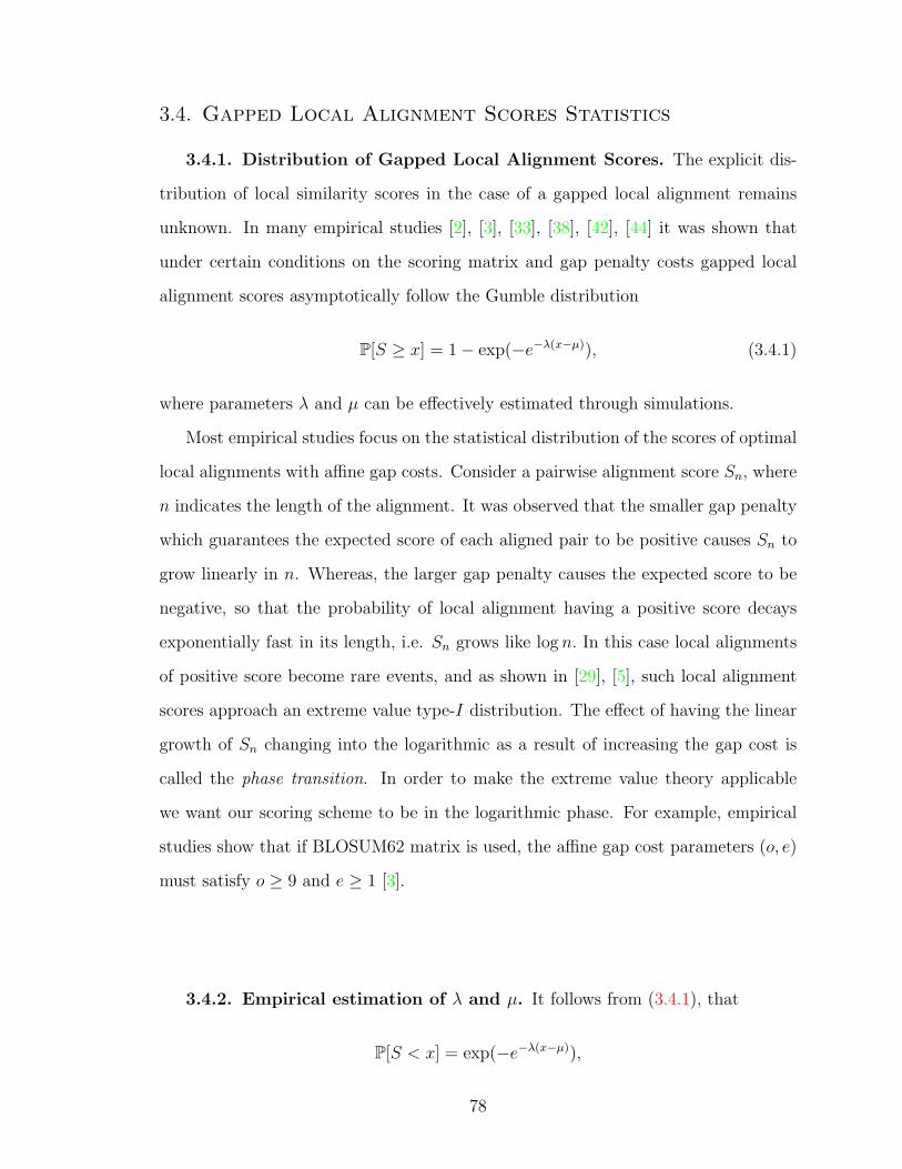
3.4. Gapped Local Alignment Scores Statistics

3.4.1. Distribution of Gapped Local Alignment Scores. The explicit dis-

tribution of local similarity scores in the case of a gapped local alignment remains

unknown. In many empirical studies [2], [3], [33], [38], [42], [44] it was shown that

under certain conditions on the scoring matrix and gap penalty costs gapped local

alignment scores asymptotically follow the Gumble distribution

P[S ≥ x] = 1− exp(−e−λ(x−µ)), (3.4.1)

where parameters λ and µ can be effectively estimated through simulations.

Most empirical studies focus on the statistical distribution of the scores of optimal

local alignments with affine gap costs. Consider a pairwise alignment score Sn, where

n indicates the length of the alignment. It was observed that the smaller gap penalty

which guarantees the expected score of each aligned pair to be positive causes Sn to

grow linearly in n. Whereas, the larger gap penalty causes the expected score to be

negative, so that the probability of local alignment having a positive score decays

exponentially fast in its length, i.e. Sn grows like log n. In this case local alignments

of positive score become rare events, and as shown in [29], [5], such local alignment

scores approach an extreme value type-I distribution. The effect of having the linear

growth of Sn changing into the logarithmic as a result of increasing the gap cost is

called the phase transition. In order to make the extreme value theory applicable

we want our scoring scheme to be in the logarithmic phase. For example, empirical

studies show that if BLOSUM62 matrix is used, the affine gap cost parameters (o, e)

must satisfy o ≥ 9 and e ≥ 1 [3].

3.4.2. Empirical estimation of λ and µ. It follows from (3.4.1), that

P[S < x] = exp(−e−λ(x−µ)),

78

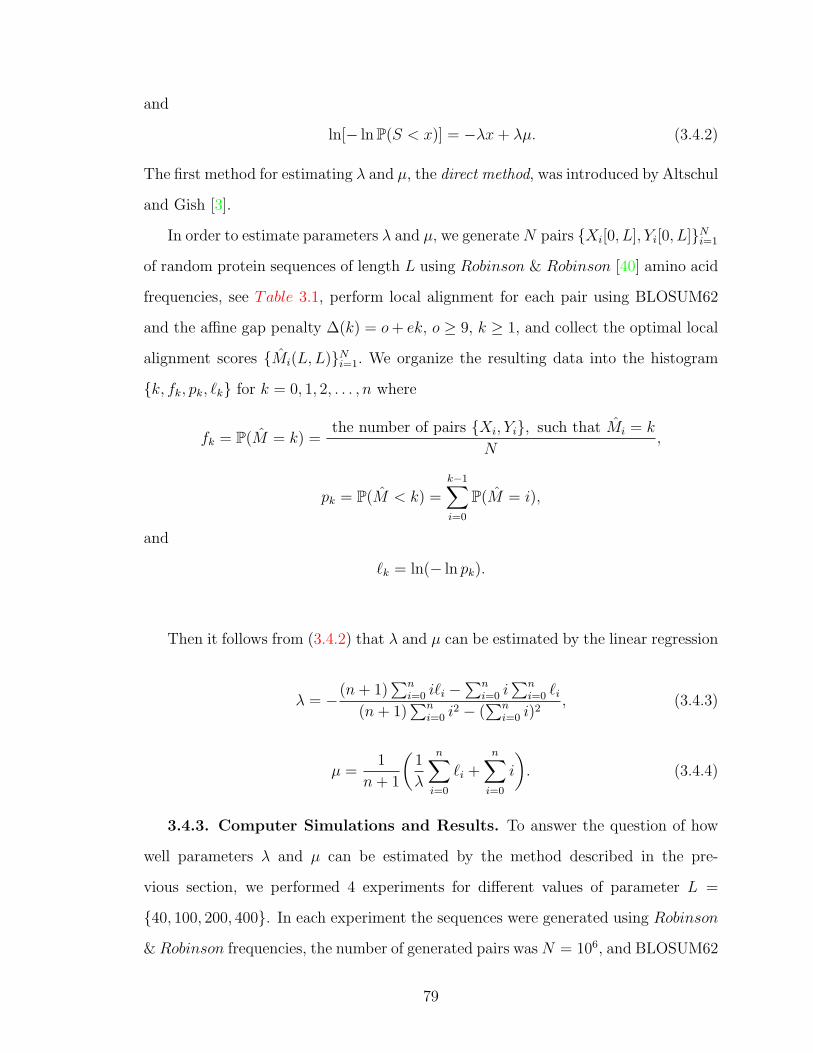
and

ln[− ln P(S < x)] = −λx+ λµ. (3.4.2)

The first method for estimating λ and µ, the direct method, was introduced by Altschul

and Gish [3].

In order to estimate parameters λ and µ, we generate N pairs Xi[0, L], Yi[0, L]Ni=1

of random protein sequences of length L using Robinson & Robinson [40] amino acid

frequencies, see Table 3.1, perform local alignment for each pair using BLOSUM62

and the affine gap penalty ∆(k) = o+ ek, o ≥ 9, k ≥ 1, and collect the optimal local

alignment scores Mi(L,L)Ni=1. We organize the resulting data into the histogram

k, fk, pk, `k for k = 0, 1, 2, . . . , n where

fk = P(M = k) =the number of pairs Xi, Yi, such that Mi = k

N,

pk = P(M < k) =k−1∑i=0

P(M = i),

and

`k = ln(− ln pk).

Then it follows from (3.4.2) that λ and µ can be estimated by the linear regression

λ = −(n+ 1)∑n

i=0 iì −∑n

i=0 i∑n

i=0 ì(n+ 1)

∑ni=0 i

2 − (∑n

i=0 i)2

, (3.4.3)

µ =1

n+ 1

(1

λ

n∑i=0

ì +n∑i=0

i

). (3.4.4)

3.4.3. Computer Simulations and Results. To answer the question of how

well parameters λ and µ can be estimated by the method described in the pre-

vious section, we performed 4 experiments for different values of parameter L =

40, 100, 200, 400. In each experiment the sequences were generated using Robinson

& Robinson frequencies, the number of generated pairs was N = 106, and BLOSUM62

79

Amino Acid R&R counts

Alanine 35155Arginine 23105

Asparagine 20212Aspartic acid 24161

Cycteine 8669Glutamic acid 19208

Glutamine 28354Glycine 33229

Histidine 9906Isoleucine 23161Leucine 40625Lysine 25872

Methionine 10101Phenylalanine 17367

Proline 23435Serine 32070

Threonine 26311Tryptophan 5990

Tyrosine 14488Valine 29012

Table 3.1. Robinson & Robinson counts among total 450431 aminoacids [40].

with the affine gap ∆(k) = −11− k, were used for scoring. In all four cases we were

able to fit the simulations data to the extreme value type-I distribution (3.4.1) with

estimated parameters λ and µ. The estimated values for λ and µ are summarized

in Table 3.2. Our results are comparable with the results obtained with more ad-

vanced methods by Hartmann [25], see Table 3.3. The details for L = 40, L = 100,

L = 200, and L = 400 are shown in Figure 3.4, F igure 3.6, F igure 3.8, F igure 3.10,

F igure 3.5, F igure 3.7, F igure 3.9, F igure 3.11.

L λ µ

40 0.348465 15.619100 0.307664 21.8939200 0.293792 26.9246400 0.282713 31.9884

Table 3.2. Simulations results.

80

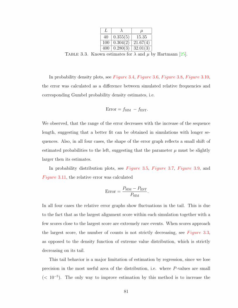
L λ µ

40 0.355(5) 15.35100 0.304(2) 21.67(4)400 0.280(3) 32.01(3)

Table 3.3. Known estimates for λ and µ by Hartmann [25].

In probability density plots, see Figure 3.4, F igure 3.6, F igure 3.8, F igure 3.10,

the error was calculated as a difference between simulated relative frequencies and

corresponding Gumbel probability density estimates, i.e.

Error = fSIM − fEST.

We observed, that the range of the error decreases with the increase of the sequence

length, suggesting that a better fit can be obtained in simulations with longer se-

quences. Also, in all four cases, the shape of the error graph reflects a small shift of

estimated probabilities to the left, suggesting that the parameter µ must be slightly

larger then its estimates.

In probability distribution plots, see Figure 3.5, F igure 3.7, F igure 3.9, and

Figure 3.11, the relative error was calculated

Error =PSIM − PEST

PSIM

.

In all four cases the relative error graphs show fluctuations in the tail. This is due

to the fact that as the largest alignment score within each simulation together with a

few scores close to the largest score are extremely rare events. When scores approach

the largest score, the number of counts is not strictly decreasing, see Figure 3.3,

as opposed to the density function of extreme value distribution, which is strictly

decreasing on its tail.

This tail behavior is a major limitation of estimation by regression, since we lose

precision in the most useful area of the distribution, i.e. where P -values are small

(< 10−5). The only way to improve estimation by this method is to increase the

81

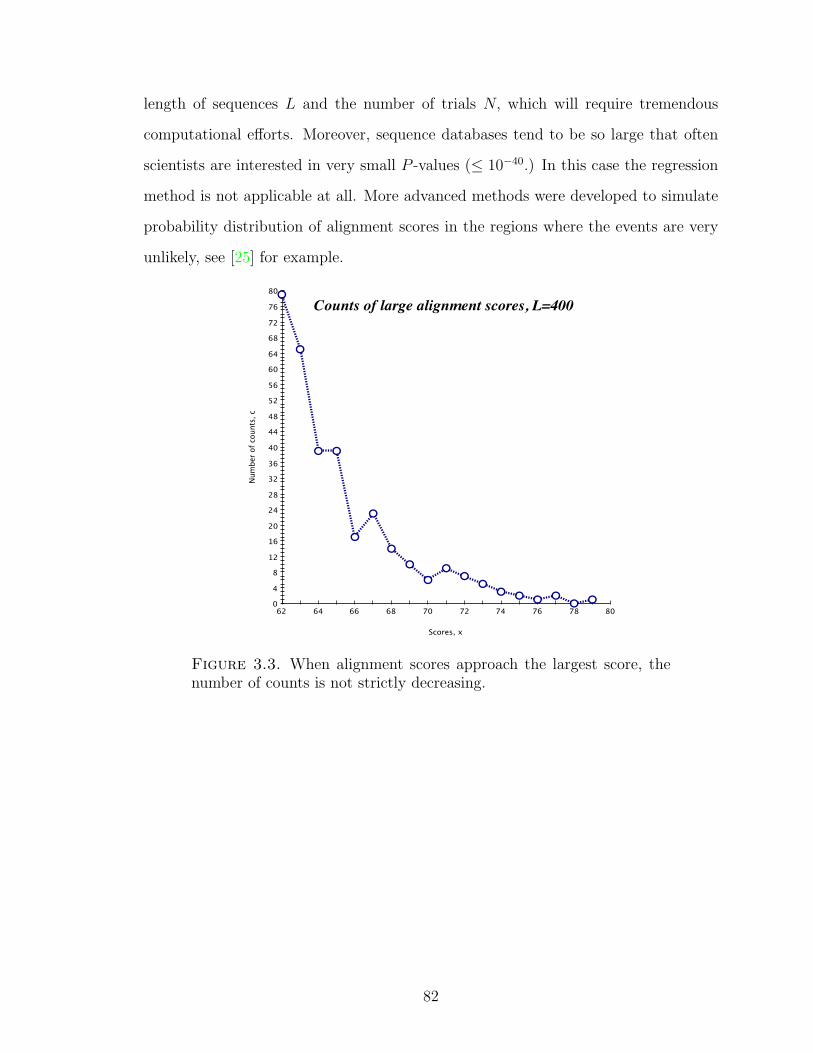
length of sequences L and the number of trials N, which will require tremendous

computational efforts. Moreover, sequence databases tend to be so large that often

scientists are interested in very small P -values (≤ 10−40.) In this case the regression

method is not applicable at all. More advanced methods were developed to simulate

probability distribution of alignment scores in the regions where the events are very

unlikely, see [25] for example.

8062 64 66 68 70 72 74 76 78

80

0

4

8

12

16

20

24

28

32

36

40

44

48

52

56

60

64

68

72

76

Scores, x

Num

ber o

f cou

nts,

c

Counts of large alignment scores, L=400

Figure 3.3. When alignment scores approach the largest score, thenumber of counts is not strictly decreasing.

82

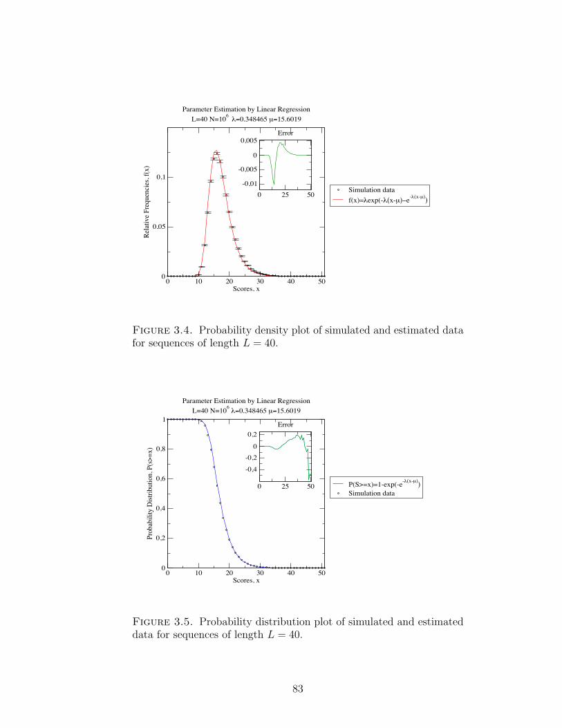
0 10 20 30 40 50Scores, x

0

0,05

0,1

Rela

tive F

requ

enci

es, f

(x)

Simulation dataf(x)=!exp(-!(x-µ)"e-!(x-µ)

)

Parameter Estimation by Linear RegressionL=40 N=106

!=0.348465 µ=15.6019

0 25 50-0,01

-0,005

0

0,005Error

Figure 3.4. Probability density plot of simulated and estimated datafor sequences of length L = 40.

0 10 20 30 40 50Scores, x

0

0,2

0,4

0,6

0,8

1

Prob

abili

ty D

istrib

utio

n, P

(s>=

x)

P(S>=x)=1-exp(-e-!(x-µ))

Simulation data


!=0.348465 µ=15.6019

0 25 50

-0,4

-0,20

0,2Error

Figure 3.5. Probability distribution plot of simulated and estimateddata for sequences of length L = 40.

83

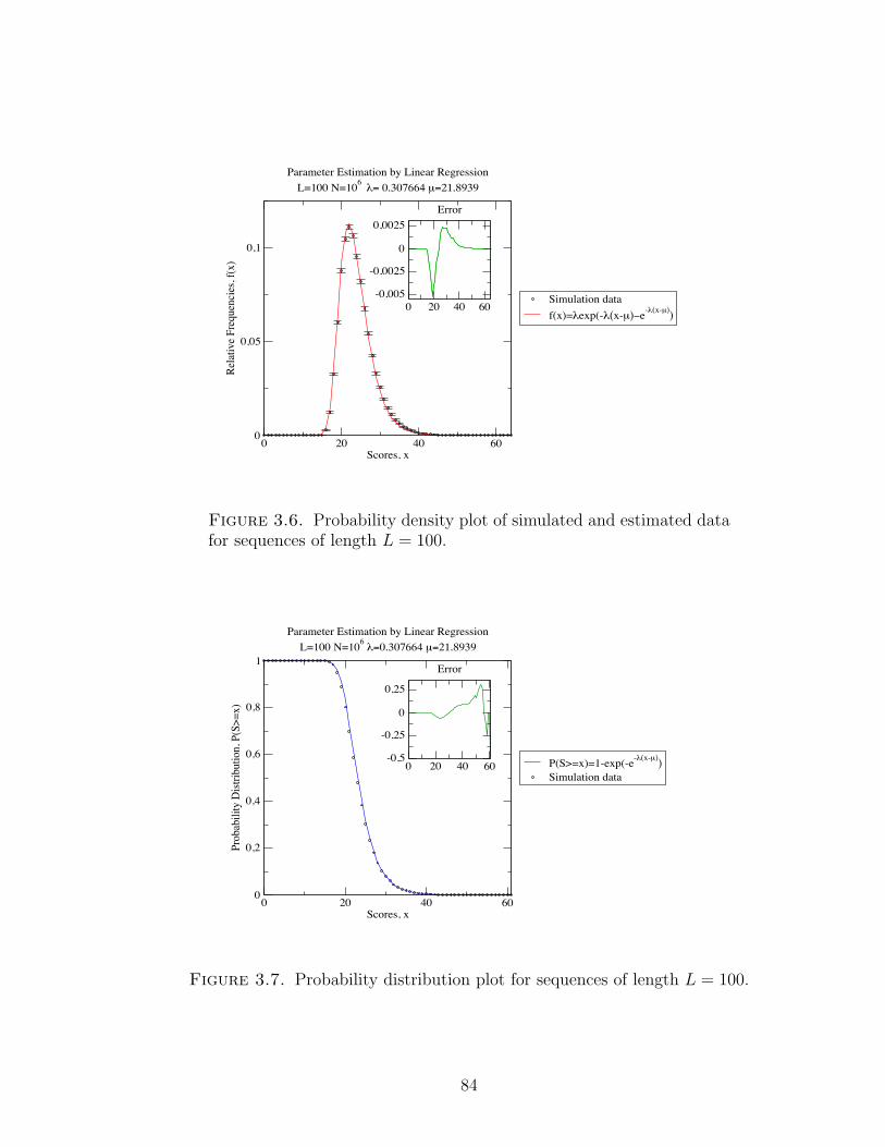
0 20 40 60Scores, x

0

0,05

0,1Re

lativ

e Fre

quen

cies

, f(x

)


)


!= 0.307664 µ=21.8939

0 20 40 60-0,005

-0,0025

0

0,0025Error


0 20 40 60Scores, x

0

0,2

0,4

0,6

0,8

1

Prob

abili

ty D

istrib

utio

n, P

(S>=

x)

P(S>=x)=1-exp(-e-!(x-µ))

Simulation data


!=0.307664 µ=21.8939

0 20 40 60-0,5

-0,25

0

0,25

Error

Figure 3.7. Probability distribution plot for sequences of length L = 100.

84

0 35 70Scores, x

0

0,05

0,1Re

lativ

e Fre

quen

cies

, f(x

)


)


!= 0.293792 µ=26.9246

0 35 70-0,004

-0,002

0

0,002Error


0 35 70Scores, x

0

0,2

0,4

0,6

0,8

1

Prob

abili

ty D

istrib

utio

n, P

(S>=

x)

P(S>=x)=1-exp(-e-!(x-µ))

Simulation data


!=0.293792 µ=26.9246

0 35 70-1,2-0,9-0,6-0,3

00,3

Error


85

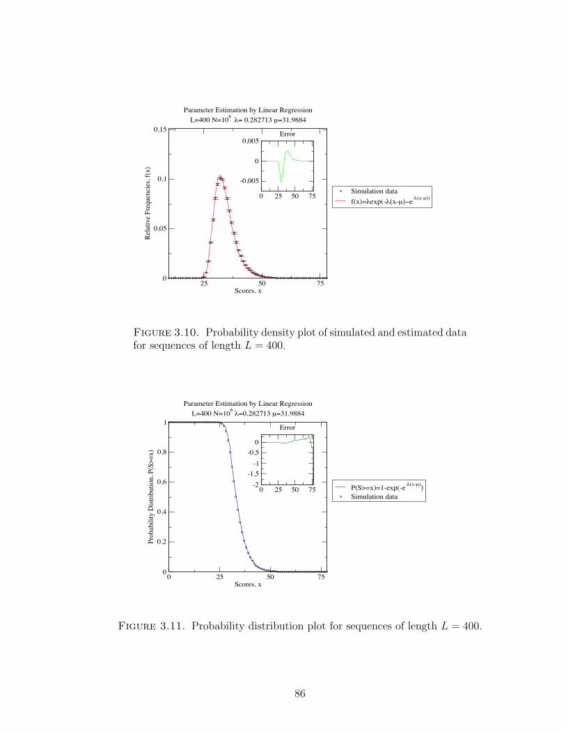
25 50 75Scores, x

0

0,05

0,1

0,15

Rela

tive F

requ

enci

es, f

(x)

Simulation dataf(x)=!exp(-!(x-µ)"e-!(x-µ))


!= 0.282713 µ=31.9884

0 25 50 75

-0,005

0

0,005Error


0 25 50 75Scores, x

0

0,2

0,4

0,6

0,8

1

Prob

abili

ty D

istrib

utio

n, P

(S>=

x)

P(S>=x)=1-exp(-e-!(x-µ))

Simulation data


!=0.282713 µ=31.9884

0 25 50 75-2

-1,5-1

-0,50

Error


86

Chapter 4

Conclusions

Recent discoveries in molecular biology revealed new facts about the structure of

biological sequences allowing biological research to become more theoretical. Namely,

there is an opportunity to study the structure and the function of biological sequences

via sequence comparison methods. Here we studied sequence alignment, a powerful

method for biosequence comparison. This method effectively combines knowledge

from biology, mathematics, computer science, and statistics. We illustrated that dy-

namic programming algorithms are effective computational tools for sequence align-

ment, and statistical methods are essential in determining the significance of align-

ment scores.

The extreme value theory proved to be very useful in the statistics of sequence

alignment. It plays the central role in the explicit formula for distribution of ungapped

local alignment scores. It also gives a good approximation in the case of gapped

local alignments. To illustrate this fact in more detail we performed simulations and

estimated parameters of extreme value type-I distribution for gapped local alignment

scores by linear regression, the most simple and straightforward method known. The

advantage of this method is a combination of simplicity and very good estimates in the

regions of distribution, where probabilities are relatively large. However, this method

it is not effective if we are specifically interested in very small probabilities, which is

often the case in biological research. Thus, for estimation of small probabilities more

advanced methods have to be used [25].

Although many results have already been obtained in the area of assessment

of statistical significance of biosequence analysis, many important questions remain

87

open. For example, explicit theory for distribution of gapped local alignment scores

and general efficient methods for global alignments are still absent [32].

Finally, we must remember that besides providing interesting mathematical and

computational research problems, biological sequence comparison helps answering

very important biological questions such as gene regulation in living organisms, evo-

lution, etc. With a deeper understanding of biological sequences and the roles they

play in living organisms, scientists will be better positioned to develop tools and

technologies that improve human health [21].

88

Bibliography

1. S. F. Altschul, Gap costs for multiple sequence alignment, J. Theor. Biol. 138 (1989Jun),

297–309.

2. S. F. Altschul, R. Bundschuh, R. Olsen, and T. Hwa, The estimation of statistical parameters

for local alignment score distributions, Nucleic Acids Res. 29 (2001Jan), 351–361.

3. S. F. Altschul and W. Gish, Local alignment statistics, Meth. Enzymol. 266 (1996), 460–480.

4. S. F. Altschul, W. Gish, W. Miller, E. W. Myers, and D. J. Lipman, Basic local alignment

search tool, J. Mol. Biol. 215 (1990Oct), 403–410.

5. R. Arratia, L. Gordon, and M.S. Waterman, The Erdos-Renyi law in distribution, for coin

tossing and sequence matching, Ann. Stat. 18 (1990), 539–570.

6. M. P. Ball, Dna chemical structure — Wikimedia Commons, http://commons.wikimedia.

org/wiki/File:DNA_chemical_structure.svg. [Online; accessed April-2010].

7. , Genetic code — Wikimedia Commons, http://commons.wikimedia.org/wiki/File:

Genetic_code.svg, 2006. [Online; accessed April-2010].

8. L. J. Beamer and C. O. Pabo, Refined 1.8 A crystal structure of the lambda repressor-operator

complex, J. Mol. Biol. 227 (1992Sep), 177–196.

9. S. A. Benner, M. A. Cohen, and G. H. Gonnet, Empirical and structural models for inser-

tions and deletions in the divergent evolution of proteins, J. Mol. Biol. 229 (1993Feb), 1065–1082.

89

http://commons.wikimedia.org/wiki/File:DNA_chemical_structure.svg

http://commons.wikimedia.org/wiki/File:DNA_chemical_structure.svg

http://commons.wikimedia.org/wiki/File:Genetic_code.svg

http://commons.wikimedia.org/wiki/File:Genetic_code.svg

10. K. M. Chao and L. Zhang, Sequence Comparison. Theory and Methods, Springer, 2009.

11. E. Chargaff, S. Zamenhof, and C. Green, Composition of human desoxypentose nucleic acid,

Nature 165 (1950May), 756–757.

12. J. E. Cohen, Mathematics is biology’s next microscope, only better; biology is mathematics’ next

physics, only better, PLoS Biol. 2 (2004Dec), 439.

13. T. Cormen, C. Leiserson, R. Rivest, and C. Stein, Introduction to Algorithms, 3rd ed., MIT

Press, 2009.

14. F. Crick, Life Itself. Its Origin and Nature, Simon and Shuster, 1995.

15. A. Dembo, S. Karlin, and O. Zeitouni, Critical phenomena for sequence matching with scoring,

Ann. Probab. 22 (1994), 1993–2021.

16. , Limit distribution of maximal non-aligned two sequence segmental score, Ann. Probab.

22 (1994), 2022–2039.

17. R. F. Doolittle, M. W. Hunkapiller, L. E. Hood, S. G. Devare, K. C. Robbins, S. A. Aaronson,

and H. N. Antoniades, Simian sarcoma virus onc gene, v-sis, is derived from the gene (or

genes) encoding a platelet-derived growth factor, Science 221 (1983Jul), 275–277.

18. R. Durbin, S. Eddy, A. Krogh, and G. Mitchison, Biological Sequence Analysis: Probabilistic

Models of Proteins and Nucleic Acids, Cambridge University Press, 1999.

19. S. R. Eddy, Where did the BLOSUM62 alignment score matrix come from?, Nat. Biotechnol.

22 (2004Aug), 1035–1036.

20. Feller, An Introduction to Probability Theory and Its Applications, 2nd ed., Vol. 2, John Wiley

and Sons, New York, 1987.

90

21. Progress from The National Institute of General Medical Sciences, Genes — what we knew,

know and hope to learn, http://www.nigms.nih.gov/Publications/FactSheet_Genes.htm.

[Online; accessed April-2010].

22. O. Gotoh, An improved algorithm for matching biological sequences, J. Mol. Biol. 162 (1982Dec),

705–708.

23. G. Grimmett and D. Stirzaker, Probability and Random Processes, 3rd ed., Oxford University

Press Inc., New York, 2001.

24. Rost Hannes, Central dogma of molecular biology — Wikimedia Commons, http:

//commons.wikimedia.org/wiki/File:BLOSUM62.gif, 2008. [Online; accessed April-2010].

25. A. K. Hartmann, Sampling rare events: statistics of local sequence alignments, Phys Rev E Stat

Nonlin Soft Matter Phys 65 (2002May), 056102.

26. S. Henikoff and J. G. Henikoff, Automated assembly of protein blocks for database searching,

Nucleic Acids Res. 19 (1991Dec), 6565–6572.

27. , Amino acid substitution matrices from protein blocks, Proc. Natl. Acad. Sci. U.S.A. 89

(1992Nov), 10915–10919.

28. N. Hulo, A. Bairoch, V. Bulliard, L. Cerutti, E. De Castro, P. S. Langendijk-Genevaux, M.

Pagni, and C. J. Sigrist, The PROSITE database, Nucleic Acids Res. 34 (2006Jan), 227–230.

29. S. Karlin and S. F. Altschul, Methods for assessing the statistical significance of molecular

sequence features by using general scoring schemes, Proc. Natl. Acad. Sci. U.S.A. 87 (1990Mar),

2264–2268.

30. , Applications and statistics for multiple high-scoring segments in molecular sequences,

Proc. Natl. Acad. Sci. U.S.A. 90 (1993Jun), 5873–5877.

91

http://www.nigms.nih.gov/Publications/FactSheet_Genes.htm

http://commons.wikimedia.org/wiki/File:BLOSUM62.gif

http://commons.wikimedia.org/wiki/File:BLOSUM62.gif

31. S. Karlin and A. Dembo, Limit distributions of maximal segmental score among markov-

dependent partial sums, Adv. Apl. Prob. 24 (1992), 113–140.

32. A. Yu. Mitrophanov and M. Borodovsky, Statistical significance in biological sequence analysis,

Briefings in Bioinformatics (2006), 2–24.

33. R. Mott, Accurate formula for P-values of gapped local sequence and profile alignments, J. Mol.

Biol. 300 (2000Jul), 649–659.

34. S. B. Needleman and C. D. Wunsch, A general method applicable to the search for similarities

in the amino acid sequence of two proteins, J. Mol. Biol. 48 (1970Mar), 443–453.

35. United States Department of Energy, Dna complementarity — Wikimedia Commons,

http://commons.wikimedia.org/wiki/File:Dna-split.png. [Online; accessed April-2010].

36. L. Pachter and B. Sturmfels, Algebraic Statistics for Computational Biology, Cambridge

University Press, 2005.

37. Y. Park, S. Sheetlin, and J. Spouge, Accelerated convergence and robust asymptotic regression of

the Gumbel scale parameter for gapped sequence alignment, J. Phys. A: Math. Gen. 38 (2005),

97–108.

38. W. R. Pearson, Empirical statistical estimates for sequence similarity searches, J. Mol. Biol.

276 (1998Feb), 71–84.

39. R. Rifkind and C. Rifkind, Naturally Obsessed: The Making of A Scientist, http:

//naturallyobsessed.com/.

40. A. B. Robinson and L. R. Robinson, Distribution of glutamine and asparagine residues and

their near neighbors in peptides and proteins, Proc. Natl. Acad. Sci. U.S.A. 88 (1991Oct),

8880–8884.

92

http://commons.wikimedia.org/wiki/File:Dna-split.png

http://naturallyobsessed.com/

http://naturallyobsessed.com/

41. T. F. Smith and M. S. Waterman, Identification of common molecular subsequences, J. Mol.

Biol. 147 (1981Mar), 195–197.

42. T. F. Smith, M. S. Waterman, and C. Burks, The statistical distribution of nucleic acid

similarities, Nucleic Acids Res. 13 (1985Jan), 645–656.

43. F. Spitzer, Principles of Random Walk, 2nd ed., Springer Verlag, New York, Berlin, Heidenberg,

2001.

44. M. S. Waterman and M. Vingron, Rapid and accurate estimates of statistical significance for

sequence data base searches, Proc. Natl. Acad. Sci. U.S.A. 91 (1994May), 4625–4628.

45. R. Wheeler, The lambda repressor-operator complex 1LMB, http://en.wikipedia.org/wiki/

User:Zephyris. [Online; accessed April-2010].

46. Wikipedia, Carbon — Wikipedia, the free encyclopedia, http://en.wikipedia.org/wiki/

Carbon. [Online; accessed April-2010].

47. , Hypothetical types of biochemistry — Wikipedia, the free encyclopedia,

http://en.wikipedia.org/wiki/Hypothetical_types_of_biochemistry. [Online; ac-

cessed April-2010].

48. , Neznaika — Wikipedia, the free encyclopedia, http://en.wikipedia.org/wiki/

Neznaika. [Online; accessed April-2010].

49. M. A. Zachariah, G. E. Crooks, S. R. Holbrook, and S. E. Brenner, A generalized affine gap

model significantly improves protein sequence alignment accuracy, Proteins 58 (2005Feb),

329–338.

93

http://en.wikipedia.org/wiki/User:Zephyris

http://en.wikipedia.org/wiki/User:Zephyris

http://en.wikipedia.org/wiki/Carbon

http://en.wikipedia.org/wiki/Carbon

http://en.wikipedia.org/wiki/Hypothetical_types_of_biochemistry

http://en.wikipedia.org/wiki/Neznaika

http://en.wikipedia.org/wiki/Neznaika

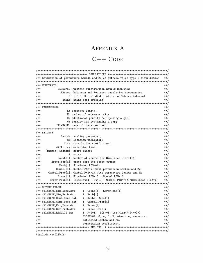
Appendix A

C++ Code

/***********************************************************************************/

/******************************** SIMULATIONS **************************************/

/** Estimation of parameters Lambda and Mu of extreme value type-I distribution **/

/***********************************************************************************/

/** CONSTANTS: **/

/** BLOSUM62: protein substitution matrix BLOSUM62 **/

/** RRfreq: Robinson and Robinson cumulative frequencies **/

/** C: [-C,C] Normal distribution confidence interval **/

/** amino: amino acid ordering **/

/***********************************************************************************/

/** PARAMETERS: **/

/** L: sequence length; **/

/** N: number of sequence pairs; **/

/** O: additional penalty for opening a gap; **/

/** e: penalty for continuing a gap; **/

/** fileNAME: name of the experiment; **/

/***********************************************************************************/

/** RETURNS: **/

/** Lambda: scaling parameter; **/

/** Mu: location parameter; **/

/** Corr: correlation coefficient; **/

/** diffclock: execution time; **/

/** [indmin, indmax]: score range; **/

/** i: score **/

/** Count[i]: number of counts (or Simulated P(S=i)*N) **/

/** Error_bar[i]: error bars for score counts **/

/** Prob[i]: Simulated P(S<=i) **/

/** Gumbel[i]: Gumbel P(S=i) with parameters Lambda and Mu **/

/** Gumbel_Prob[i]: Gumbel P(S<=i) with parameters Lambda and Mu **/

/** Error[i]: Simulated P(S=i) - Gumbel P(S=i) **/

/** Error_Prob[i]: (Simulated P(S<=i) - Gumbel P(S<=i))/Simulated P(S<=i) **/

/***********************************************************************************/

/** OUTPUT FILES: **/

/** fileNAME_Sim_Dens.dat i Count[i] Error_bar[i] **/

/** fileNAME_Sim_Prob.dat i Prob[i] **/

/** fileNAME_Gumb_Dens.dat i Gumbel_Dens[i] **/

/** fileNAME_Gumb_Prob.dat i Gumbel_Prob[i] **/

/** fileNAME_Err_Dens.dat i Error[i] **/

/** fileNAME_Err_Prob.dat i Error_Prob[i] **/

/** fileNAME_RESULTS.dat i P(S=i) P(S<=i) log(-log(P(S<=y))) **/

/** BLOSUM62, O, e, L, N, minscore, maxscore, **/

/** estimated Lambda and Mu, **/

/** correlation coefficient. **/

/********************************* THE END :) **************************************/

/***********************************************************************************/

#include <stdlib.h>

94

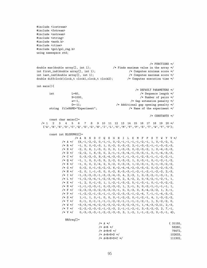
#include <iostream>

#include <fstream>

#include <sstream>

#include <string>

#include <math.h>

#include <ctime>

#include <gsl/gsl_rng.h>

using namespace std;

/* FUNCTIONS */

double max(double array[], int l); /* Finds maximum value in the array */

int first_ind(double array[], int l); /* Computes minimum score */

int last_ind(double array[], int l); /* Computes maximum score */

double diffclock(clock_t clock1,clock_t clock2); /* Computes execution time */

int main()

/* DEFAULT PARAMETERS */

int L=40, /* Sequence length */

N=1000, /* Number of pairs */

e=-1, /* Gap extension penalty */

O=-11; /* Additional gap opening penalty */

string fileNAME="Experiment"; /* Name of the experiment */

/* CONSTANTS */

const char amino[]=

/* 1 2 3 4 5 6 7 8 9 10 11 12 13 14 15 16 17 18 19 20 */

’A’,’R’,’N’,’D’,’C’,’Q’,’E’,’G’,’H’,’I’,’L’,’K’,’M’,’F’,’P’,’S’,’T’,’W’,’Y’,’V’;

const int BLOSUM62[]=

/* A R N D C Q E G H I L K M F P S T W Y V */

/* A */ 4,-1,-2,-2, 0,-1,-1, 0,-2,-1,-1,-1,-1,-2,-1, 1, 0,-3,-2, 0,

/* R */ -1, 5, 0,-2,-3, 1, 0,-2, 0,-3,-2, 2,-1,-3,-2,-1,-1,-3,-2,-3,

/* N */ -2, 0, 6, 1,-3, 0, 0, 0, 1,-3,-3, 0,-2,-3,-2, 1, 0,-4,-3,-3,

/* D */ -2,-2, 1, 6,-3, 0, 2,-1,-1,-3,-4,-1,-3,-3,-1, 0,-1,-4,-3,-3,

/* C */ 0,-3,-3,-3, 9,-3,-4,-3,-3,-1,-1,-3,-1,-2,-3,-1,-1,-2,-2,-1,

/* Q */ -1, 1, 0, 0,-3, 5, 2,-2, 0,-3,-2, 1, 0,-3,-1, 0,-1,-2,-1,-2,

/* E */ -1, 0, 0, 2,-4, 2, 5,-2, 0,-3,-3, 1,-2,-3,-1, 0,-1,-3,-2,-2,

/* G */ 0,-2, 0,-1,-3,-2,-2, 6,-2,-4,-4,-2,-3,-3,-2, 0,-2,-2,-3,-3,

/* H */ -2, 0, 1,-1,-3, 0, 0,-2, 8,-3,-3,-1,-2,-1,-2,-1,-2,-2, 2,-3,

/* I */ -1,-3,-3,-3,-1,-3,-3,-4,-3, 4, 2,-3, 1, 0,-3,-2,-1,-3,-1, 3,

/* L */ -1,-2,-3,-4,-1,-2,-3,-4,-3, 2, 4,-2, 2, 0,-3,-2,-1,-2,-1, 1,

/* K */ -1, 2, 0,-1,-3, 1, 1,-2,-1,-3,-2, 5,-1,-3,-1, 0,-1,-3,-2,-2,

/* M */ -1,-1,-2,-3,-1, 0,-2,-3,-2, 1, 2,-1, 5, 0,-2,-1,-1,-1,-1, 1,

/* F */ -2,-3,-3,-3,-2,-3,-3,-3,-1, 0, 0,-3, 0, 6,-4,-2,-2, 1, 3,-1,

/* P */ -1,-2,-2,-1,-3,-1,-1,-2,-2,-3,-3,-1,-2,-4, 7,-1,-1,-4,-3,-2,

/* S */ 1,-1, 1, 0,-1, 0, 0, 0,-1,-2,-2, 0,-1,-2,-1, 4, 1,-3,-2,-2,

/* T */ 0,-1, 0,-1,-1,-1,-1,-2,-2,-1,-1,-1,-1,-2,-1, 1, 5,-2,-2, 0,

/* W */ -3,-3,-4,-4,-2,-2,-3,-2,-2,-3,-2,-3,-1, 1,-4,-3,-2,11, 2,-3,

/* Y */ -2,-2,-2,-3,-2,-1,-2,-3, 2,-1,-1,-2,-1, 3,-3,-2,-2, 2, 7,-1,

/* V */ 0,-3,-3,-3,-1,-2,-2,-3,-3, 3, 1,-2, 1,-1,-2,-2, 0,-3,-1, 4,

RRfreq[]=

/* A */ 31155,

/* A+R */ 58260,

/* A+R+N */ 78472,

/* A+R+N+D */ 102633,

/* A+R+N+D+C */ 111302,

95

/* A+R+N+D+C+Q */ 130510,

/* A+R+N+D+C+Q+E */ 158864,

/* A+R+N+D+C+Q+E+G */ 192093,

/* A+R+N+D+C+Q+E+G+H */ 201999,

/* A+R+N+D+C+Q+E+G+H+I */ 225160,

/* A+R+N+D+C+Q+E+G+H+I+L */ 265785,

/* A+R+N+D+C+Q+E+G+H+I+L+K */ 291657,

/* A+R+N+D+C+Q+E+G+H+I+L+K+M */ 301758,

/* A+R+N+D+C+Q+E+G+H+I+L+K+M+F */ 319125,

/* A+R+N+D+C+Q+E+G+H+I+L+K+M+F+P */ 342560,

/* A+R+N+D+C+Q+E+G+H+I+L+K+M+F+P+S */ 374630,

/* A+R+N+D+C+Q+E+G+H+I+L+K+M+F+P+S+T */ 400941,

/* A+R+N+D+C+Q+E+G+H+I+L+K+M+F+P+S+T+W */ 406931,

/* A+R+N+D+C+Q+E+G+H+I+L+K+M+F+P+S+T+W+Y */ 421419,

/* A+R+N+D+C+Q+E+G+H+I+L+K+M+F+P+S+T+W+Y+V */450431,

Num_score=100;

const double C=1.96; /* Normal distribution 95% confidence interval*/

int i /* Score */

j,q,

ind,

MaxScore, /* Maximum score in local pairwise alignment */

indmin,indmax;

double rnd,

Count[Num_score], /* Simulated score frequencies */

Prob[Num_score], /* Simulated cumulative probability */

Prob1[Num_score],

Error_bar[Num_score], /* Error bars for counting scores (5%) */

Sx, Sy, Sxy, Sx2, /* Regression sums */

Sy2, Sn,

Corr, /* Correlation coefficient */

Lambda, Mu, /* Estimated parameters */

Gumbel[Num_score], /* Estimated probability density */

Gumbel_Prob[Num_score], /* Estimated cumulative probability */

Error[Num_score], /* Errors */

Error_Prob[Num_score];

string file1,file2,file3,

file4,file5,file6,

file7;

clock_t before=clock();

cout<< "********************************************************************"<<endl;

cout<< "** WELCOME TO THE GAPPED LOCAL ALIGNMENT STATISTICS SIMULATIONS! **"<<endl;

cout<< "********************************************************************"<<endl;

cout<< "******************* DEFAULT PARAMETERS: ****************************"<<endl;

cout<< "Substitution matrix: BLOSUM62"<<endl;

cout<< "Affine gap penalty: O = "<<O<<" and e = "<<e<<endl;

cout<< "Sequence length: L = "<<L<<endl;

cout<< "Number of sequence pairs : N = "<<N<<endl;

cout<< "Name of the experiment : "<<fileNAME<<endl;

cout<< "********************************************************************"<<endl;

char Ans;

int Par;

cout<< "Would you like to reset parameters (Y/N)? ";

cin >> Ans;

if(Ans == ’Y’ || Ans == ’y’ )

cout << "Sequence length, L = ";

96

cin >> Par;

L=Par;

cout << "Number of pairs, N = ";

cin >> Par;

N=Par;

cout << "Penalty for opening a gap, O = ";

cin >> Par;

O=Par;

cout << "Penalty for extending a gap, e = ";

cin >> Par;

e=Par;

cout << "Name of the experiment: ";

cin >> fileNAME;

;

char Seq[2*L]; /* Amino acid representation of pair of sequences */

int Seq_Num[2*L]; /* Integer representation of pair of sequences */

double

S[(L+1)*(L+1)], /* Substitution, Deletion, and Insertion matrices */

D[(L+1)*(L+1)],

I[(L+1)*(L+1)],

rec_S[4], /* Recursion arrays */

rec_D[2],

rec_I[2],

gsl_rng *rng; /* Initialization of pseudorandom number generator */

srand((unsigned)time(0)); /* We used mt19937 from GSL library */

rng=gsl_rng_alloc(gsl_rng_mt19937);

gsl_rng_set(rng, rand());

for (i=0;i<Num_score;i++)

Count[i]=0;

for (q=1;q<=N;q++)

for(i=0;i<2*L;i++) /* Generating a pair of random protein sequences*/

rnd=gsl_rng_uniform(rng)*450431;

if (rnd<=RRfreq[0])Seq[i]=amino[0];Seq_Num[i]=0;

for (j=1;j<=20;j++)

if (rnd<=RRfreq[j]&&rnd>=RRfreq[j-1])

Seq[i]=amino[j]; Seq_Num[i]=j;

/* Aligning sequences by SMITH-WATERMAN ALGORITHM (affine gap) */

for(i=0;i<=L-1;i++) /* Initialization */

for (j=0;j<=L-1;j++)

S[i*L+j]=0;

D[i*L+j]=0;

I[i*L+j]=0;

for (i=0;i<=L;i++)

D[i*L]=-100;

I[i*L]=-100;

S[i*L]=0;

for (j=0;j<=L;j++)

I[j]=-100;

D[j]=-100;

S[j]=0;

97

for (i=1;i<=L;i++) /* Recursion */

for (j=1;j<=L;j++)

ind=(Seq_Num[i-1])*20+Seq_Num[L+j-1];

rec_S[0]=S[(i-1)*L+j-1]+BLOSUM62[ind];

rec_S[1]=D[(i-1)*L+j-1]+BLOSUM62[ind];

rec_S[2]=I[(i-1)*L+j-1]+BLOSUM62[ind];

rec_S[3]=0;

S[i*L+j]=max(rec_S,4);

rec_D[0]=S[(i-1)*L+j]+O+e;

rec_D[1]=D[(i-1)*L+j]+e;

D[i*L+j]=max(rec_D,2);

rec_I[0]=S[i*L+j-1]+O+e;

rec_I[1]=I[i*L+j-1]+e;

I[i*L+j]=max(rec_I,2);

MaxScore=0; /* Finding maximum score */

for (i=1;i<=L;i++)

for (j=1;j<=L;j++)

if(S[L*i+j]>MaxScore)

MaxScore = S[L*i+j];

if (MaxScore>=0&&MaxScore<Num_score) /* Counting maximum score */

Count[MaxScore]++;

Prob[0]=0; /* Calculating frequencies, error bars and probabilities */

Prob1[0]=log(-1*(log(Prob[0])));

Error_bar[0]=(sqrt(Count[0]*(1-(Count[0]/N)))*C*2)/N;

for(i=1;i<Num_score;i++)

Error_bar[i]=(sqrt(Count[i]*(1-(Count[i]/N)))*C*2)/N;

Prob[i]=Prob[i-1]+Count[i]/N;

Prob1[i]=log(double((-1)*log(Prob[i])));

/* Organizing output */

file1=fileNAME+"_Sim_Dens.dat";

file2=fileNAME+"_Sim_Prob.dat";

file3=fileNAME+"_Gumb_Dens.dat";

file4=fileNAME+"_Gumb_Prob.dat";

file5=fileNAME+"_Err_Dens.dat";

file6=fileNAME+"_Err_Prob.dat";

file7=fileNAME+"_RESULTS.dat";

ofstream fout1(file1.c_str(), ios::ate);







cout<< "********************************************************************"<<endl;

cout<< "********************* DISTRIBUTION OF SCORES ***********************"<<endl;

cout<< "********************************************************************"<<endl;

cout<<"y"<<’\t’<<"P(S=y)"<<’\t’<<"P(S<=y)"<<’\t’<<"log(-log(P(S<=y)))"<<endl;

fout7<< "********************************************************************"<<endl;

fout7<< "******************** DISTRIBUTION OF SCORES ************************"<<endl;

98

fout7<< "********************************************************************"<<endl;

fout7<<"y"<<’\t’<<"P(S=y)"<<’\t’<<"P(S<y)"<<’\t’<<"log(-log(P(S<y)))"<<endl;

indmin=first_ind(Count, Num_score);

indmax=last_ind(Prob, Num_score);

for(i=indmin;i<=indmax;i++)

cout<<i<<’\t’<<Count[i]/(N)<<’\t’<<Prob[i]<<’\t’<<Prob1[i]<<endl;

fout7<<i<<’\t’<<Count[i]/(N)<<’\t’<<Prob[i]<<’\t’<<Prob1[i]<<endl;

fout1<<i<<" "<<Count[i]/(N)<<" "<<Error_bar[i]<<endl;

fout2<<i<<" "<<1-Prob[i]<<endl;

Sy=Prob1[indmin]; /* Regression */

Sx=indmin;

Sxy=Sx*Sy;

Sx2=Sx*Sx;

Sy2=Sy*Sy;

for(i=indmin+1;i<indmax;i++)

Sy=Sy+Prob1[i];

Sx=Sx+i;

Sxy=Sxy+i*Prob1[i];

Sx2=Sx2+i*i;

Sy2=Sy2+Prob1[i]*Prob1[i];

Sn=indmax-indmin;

Lambda=-1*(Sn*Sxy-Sx*Sy)/(Sn*Sx2-Sx*Sx); /* Lambda Estimation */

Mu=(Sy+Lambda*Sx)/(Sn*Lambda); /* Mu Estimation */

Corr=(Sn*Sxy-Sx*Sy)/(sqrt(Sn*Sx2-Sx*Sx)*sqrt(Sn*Sy2-Sy*Sy));

cout<< "**************************** PARAMETERS ******************************"<<endl;

cout<<"Substitution matrix: BLOSUM62"<<endl;

cout<<"Affine gap penalty: O = "<<O<<" and e = "<<e<<endl;

cout<<"Sequence length: "<<L<<endl;

cout<<"Number of pairs: "<<N<<endl;

cout<<"Minimum score: "<<indmin<<endl;

cout<<"Maxumum score: "<<indmax<<endl;

cout<<"Regression Lambda: "<<Lambda<<endl;

cout<<"Regression Mu: "<<Mu<<endl;

cout<<"Correlation coefficient "<<Corr<<endl;

cout<< "**************************** THE END :) *******************************"<<endl;

fout7<< "**************************** PARAMETERS ******************************"<<endl;

fout7<<"Substitution matrix: BLOSUM62"<<endl;

fout7<< "Affine gap penalty: O = "<<O<<" and e = "<<e<<endl;

fout7<<"Sequence Length: "<<L<<endl;

fout7<<"Number of pairs: "<<N<<endl;

fout7<<"Minimum score: "<<indmin<<endl;

fout7<<"Maximum score: "<<indmax<<endl;

fout7<<"Regression Lambda: "<<Lambda<<endl;

fout7<<"Regression Mu: "<<Mu<<endl;

fout7<<"Correlation coefficient: "<<Corr<<endl;

fout7<< "**************************** THE END :) ******************************"<<endl;

/* Computing extreme value type-I density and distribution with parameter Lambda and Mu */

/* Computing errors between simulated and estimated data */

for (i=0;i<Num_score;i++)

Gumbel[i]=Lambda*exp(-Lambda*(i-Mu))*exp(-exp(-Lambda*(i-Mu)));

fout3<<i<<" "<<Gumbel[i]<<endl;

Gumbel_Prob[i]=1-exp(-exp(-Lambda*(i-Mu)));

fout4<<i<<" "<<Gumbel_Prob[i]<<endl;

Error[i]=Count[i]/(N)-Gumbel[i];

fout5<<i<<" "<<Error[i]<<endl;

Error_Prob[i]=(1-Prob[i]-Gumbel_Prob[i])/(1-Prob[i]);

99

fout6<<i<<" "<<Error_Prob[i]<<endl;

clock_t after=clock();

cout<<"Execution Time:"<<’\t’<<diffclock(after,before)<<" sec"<<endl;

fout7<<"Execution Time:"<<’\t’<<diffclock(after,before)<<" sec"<<endl;

fout1.close();

fout2.close();

fout3.close();

fout4.close();

fout5.close();

fout6.close();

fout7.close();

return 0;

int first_ind(double array[], int l)

int ind=0;

for (int i=0; i<l;i++)

if (array[i]>0)ind=i;break;

return ind;

int last_ind(double array[], int l)

int ind=0;

for (int i=0;i<l;i++)

if(array[l-i-1]>0) ind=l-i-1; break;

return ind;

double max(double array[], int l)

double max_val=array[0];

for (int i=1;i<l;i++)

if(array[i]>max_val)

max_val=array[i];

return max_val;

double diffclock(clock_t clock1,clock_t clock2)

double diffticks=clock1-clock2;

double diffms=(diffticks)/CLOCKS_PER_SEC;

return diffms;

100

Documents

Mathematical Models, Algorithms, and Statistics of ...people.math.sc.edu/czabarka/Theses/thesis_orlova.pdfMathematical Models, Algorithms, and Statistics of Sequence ... Alignment