MATHEMATICAL MODELS OF THE ADAPTIVE

IMMUNE RESPONSE IN A NOVEL CANCER

IMMUNOTHERAPY

by

Bryan A. Dawkins

A dissertation submitted to the faculty ofThe University of Central Oklahoma

in partial fulfillment of the requirements for the degree of

Master of Science

Department of Mathematics

The University of Central Oklahoma

May 2016

Copyright c© Bryan A. Dawkins 2016

All Rights Reserved

i

ABSTRACT

The immune system is the first line of defense against cancer. The immune system

regularly detects and destroys cancer cells. Despite this continuous protection, certain

cancers are able to escape detection or destruction by the immune system. Research in

recent decades has addressed the possibility of enlisting the help of the immune system

to detect and destroy cancer cells. One compelling treatment uses a laser, an immune

stimulant called glycated chitosan (GC), and a light absorbing dye called indocyanine

green to convince the immune system to incite a systemic attack against both primary

and metastatic tumors. In successful treatments, all tumors are completely destroyed and

patients develop long-term immunity against tumors. While attempting to locate and

destroy tumor cells, the cells of the immune system face competing pressures. On one

hand are the immune cells that detect and attempt to control tumor cells (typically the

target of the immune response is a foreign invader), and on the other hand are the immune

cells that prevent the response from growing dangerously out of control. By policing certain

immune cell populations, regulatory T cells (Tregs) play an important role in keeping the

overall immune response under control. But, in doing so, these Tregs indirectly protect

cancer cells.

We describe post-treatment immune dynamics with mathematical models, and predic-

tions of clinical treatment outcomes can be drawn from model predictions. Currently we

emphasize the role of cytotoxic T cells and dendritic cells in the laser-initiated immune

response, but we have also studied the roles of B cells and helper T cells. Our model is

based on experimental studies with the dimethylbenza(a)nthracene-4 (DMBA-4) metastatic

mammary tumor line in the rat animal model. We have used our model to determine clinical

outcomes based on the effects of two key treatment factors: the dose and role of GC, and

the manipulation of Treg activity. Treatment outcome is improved by the pro-immune

stimulatory properties of GC and worsened by the proposed pro-tumor activity of Tregs.

The results from our studies indicate potential treatment designs that could be used to

improve treatment outcome or highlight additional areas that should be targeted for future

experimentation with animal models.

I would like to dedicate this to my family and my wonderful wife. You have all been

instrumental in my development into the person I am today.

CONTENTS

ABSTRACT . . . . . . . . . . . . . . . . . . . . . . . . . . . . . . . . . . . . . . . . . . . . . . . . . . . . . . . . ii

LIST OF FIGURES . . . . . . . . . . . . . . . . . . . . . . . . . . . . . . . . . . . . . . . . . . . . . . . . . vi

LIST OF TABLES . . . . . . . . . . . . . . . . . . . . . . . . . . . . . . . . . . . . . . . . . . . . . . . . . . . vii

ACKNOWLEDGEMENTS . . . . . . . . . . . . . . . . . . . . . . . . . . . . . . . . . . . . . . . . . . . viii

CHAPTERS

1. INTRODUCTION . . . . . . . . . . . . . . . . . . . . . . . . . . . . . . . . . . . . . . . . . . . . . . . 1

1.1 Cancerous Tumor Growth . . . . . . . . . . . . . . . . . . . . . . . . . . . . . . . . . . . . . . . . 11.2 Cancer Immunotherapies . . . . . . . . . . . . . . . . . . . . . . . . . . . . . . . . . . . . . . . . . 21.3 Mathematical Models of Cancer Immunology . . . . . . . . . . . . . . . . . . . . . . . . . 21.4 Categories of Immunity . . . . . . . . . . . . . . . . . . . . . . . . . . . . . . . . . . . . . . . . . . 31.5 Dendritic Cells (DCs) . . . . . . . . . . . . . . . . . . . . . . . . . . . . . . . . . . . . . . . . . . . 31.6 T Cells . . . . . . . . . . . . . . . . . . . . . . . . . . . . . . . . . . . . . . . . . . . . . . . . . . . . . . . 4

1.6.1 Cytotoxic T Lymphocytes (CTLs) . . . . . . . . . . . . . . . . . . . . . . . . . . . . . 41.6.2 Helper T Cells . . . . . . . . . . . . . . . . . . . . . . . . . . . . . . . . . . . . . . . . . . . . . 41.6.3 Regulatory T Cells (Tregs) . . . . . . . . . . . . . . . . . . . . . . . . . . . . . . . . . . . 4

1.7 B Cells and Antibodies . . . . . . . . . . . . . . . . . . . . . . . . . . . . . . . . . . . . . . . . . . 51.8 Immunoadjuvants and Elements of Treatment . . . . . . . . . . . . . . . . . . . . . . . . 5

2. MATHEMATICAL MODEL . . . . . . . . . . . . . . . . . . . . . . . . . . . . . . . . . . . . . . 6

2.1 Mathematical Model . . . . . . . . . . . . . . . . . . . . . . . . . . . . . . . . . . . . . . . . . . . . 72.2 Parameterization . . . . . . . . . . . . . . . . . . . . . . . . . . . . . . . . . . . . . . . . . . . . . . . 10

3. ANALYSIS OF MATHEMATICAL MODEL . . . . . . . . . . . . . . . . . . . . . . . 14

3.1 Sensitivity Analysis . . . . . . . . . . . . . . . . . . . . . . . . . . . . . . . . . . . . . . . . . . . . . 153.1.1 Latin Hypercube Sampling . . . . . . . . . . . . . . . . . . . . . . . . . . . . . . . . . . . 15

3.2 Predictions of Treatment Outcomes . . . . . . . . . . . . . . . . . . . . . . . . . . . . . . . . 173.3 Modeling the Effects of Glycated Chitosan (GC) . . . . . . . . . . . . . . . . . . . . . . 213.4 Regulatory T Cell Experimental Simulation . . . . . . . . . . . . . . . . . . . . . . . . . . 24

4. DISCUSSION . . . . . . . . . . . . . . . . . . . . . . . . . . . . . . . . . . . . . . . . . . . . . . . . . . . 29

4.1 Summary . . . . . . . . . . . . . . . . . . . . . . . . . . . . . . . . . . . . . . . . . . . . . . . . . . . . . 294.2 Suggested experiments . . . . . . . . . . . . . . . . . . . . . . . . . . . . . . . . . . . . . . . . . . 30

5. FUTURE WORK . . . . . . . . . . . . . . . . . . . . . . . . . . . . . . . . . . . . . . . . . . . . . . . . 32

5.1 Modeling . . . . . . . . . . . . . . . . . . . . . . . . . . . . . . . . . . . . . . . . . . . . . . . . . . . . . 325.2 Experimentation . . . . . . . . . . . . . . . . . . . . . . . . . . . . . . . . . . . . . . . . . . . . . . . 325.3 Speculation . . . . . . . . . . . . . . . . . . . . . . . . . . . . . . . . . . . . . . . . . . . . . . . . . . . 33

APPENDICES

A. IMMUNOLOGICALLY EXPANDED MODEL . . . . . . . . . . . . . . . . . . . . . 34

B. REDUCED MODEL WITHOUT CTL PROLIFERATION . . . . . . . . . . . 36

C. MODEL OF CTL PROLIFERATION . . . . . . . . . . . . . . . . . . . . . . . . . . . . . . 37

D. NON MASS-ACTION VS. MASS-ACTION TUMOR CELL KILLING 39

REFERENCES . . . . . . . . . . . . . . . . . . . . . . . . . . . . . . . . . . . . . . . . . . . . . . . . . . . . . 40

v

LIST OF FIGURES

2.1 Conceptual model of anti-tumor laser immunotherapy. . . . . . . . . . . . . . . . . . . . 6

2.2 Predicted tumor-immune dynamics for successful treatment. . . . . . . . . . . . . . . 8

2.3 CTL progression through proliferative stages. . . . . . . . . . . . . . . . . . . . . . . . . . . 9

2.4 Parameters partitioned by innate, cancer, Treg, and GC processes. . . . . . . . . . 11

3.1 Sample stratified parameter distribution. . . . . . . . . . . . . . . . . . . . . . . . . . . . . . 15

3.2 Comparison of 2D Latin Hypercube and Simple Random Sampling. . . . . . . . . 16

3.3 (Revisited) Predicted tumor-immune dynamics for successful treatment. . . . . . 18

3.4 (Revisited) CTL progression through proliferative stages. . . . . . . . . . . . . . . . . 20

3.5 Variation in clinical outcomes across patient parameters. . . . . . . . . . . . . . . . . . 21

3.6 Variation in clinical outcomes across GC parameters. . . . . . . . . . . . . . . . . . . . . 23

3.7 Model simulation across GC parameters. . . . . . . . . . . . . . . . . . . . . . . . . . . . . . 24

3.8 Simulated cell dynamics across all clinical outcomes. . . . . . . . . . . . . . . . . . . . . 26

3.9 Variation in clinical outcomes across Treg activity parameters. . . . . . . . . . . . . 27

C.1 Comparison of CTL dynamics with and without proliferation. . . . . . . . . . . . . . 38

D.1 Comparison of tumor dynamics with CTL and without CTL proliferation. . . . 39

LIST OF TABLES

2.1 Patient parameter values, units, and references. . . . . . . . . . . . . . . . . . . . . . . . . 12

2.2 Regulatory T cell, cancer, and glycated chitosan associated parameter values,units, and references. . . . . . . . . . . . . . . . . . . . . . . . . . . . . . . . . . . . . . . . . . . . . . 13

3.1 Sample GC parameters with respect to clinical outcome. . . . . . . . . . . . . . . . . . 22

3.2 Sample Treg activity parameters with respect to clinical outcome. . . . . . . . . . . 28

ACKNOWLEDGEMENTS

• I would like to especially thank my advisor, Dr. Sean M. Laverty, for being the

reason I started doing research from the beginning of my time at UCO. When I first

stepped foot into your differential equations class as a first-semester transfer student,

I was a nervous wreck. I was terrified of failure and I never even considered the

possibility that I might write and present mathematical models in front of audiences,

let alone teach my own students. Even though I desired to do research outside the

classroom, I would have never asked anyone because I was too terrified of the idea of

possibly being rejected. When you asked me if I would be interested in doing research,

you opened the door to personal growth that I would have never achieved on my own.

You have given me so many opportunities and you have taught me so much. You have

given me advice in every major decision I have had to make in terms of my future

direction. My hope is that I will one day be able to make an impact in a student’s life

like you have impacted mine. I will be forever grateful to you for all you have done

for me.

• To Dr. Brittany E. Bannish, I would like to thank you for always helping me

extend my knowledge by asking difficult questions regarding the work I have done as I

have presented it to you. There were many times when you asked me questions I had

not yet considered, which led me to dig deeper into the literature or go back to the

drawing board so I could figure things out. Thank you for always being encouraging

and for giving me much needed advice about graduate school and what to expect as

my future unfolds.

• Dr. Wei R. Chen and the entire Biophotonics Research Laboratory are the

reason the topic of my research even exists. I have been fascinated by your work from

the first time I initially read one of your published papers. Since then, I have learned

so much and I have great appreciation for the complexity of immunological responses

to cancer. Thank you for making my research possible.

• I would like to thank Dr. Charles L. Cooper for enhancing my appreciation and

understanding of mathematics. Thank you for enlightening me on what mathematics

is and what it is not. Also, thank you for always challenging your students to think

critically to become better problem solvers.

• I would like to thank Dr. Tracy L. Morris for being such a hard working, helpful

teacher. Thank you for asking questions and offering your help on my project at the

late stage it was in.

• Thank you to all of the Mathematics and Statistics faculty for being wonderful

teachers and for being so involved with your students. The UCO Math and Stat

Department is like a family. You all work so well together and it makes the entire

operation more effective. You all are what makes the university the wonderful place

that it is.

• Without the RCSA grant program and CURE-STEM at UCO, I would have

never been able to do productive research for financial reasons. This program provided

me with the time that I needed to accomplish difficult research tasks throughout my

entire time at UCO.

• Thank you to my entire family who has supported me throughout my entire life.

Thank you to my wonderful wife, Grace, who has been so encouraging and by my side

in everything I do.

ix

CHAPTER 1

INTRODUCTION

To begin our work mathematically modeling a potential mechanism underlying a novel

anti-tumor immunotherapy, we give a brief introduction to cancerous tumor growth, cancer

immunotherapies, existing cancer models, and immunology. The activities of the immune

system cells listed are not limited to anti-tumor immunity. However, the descriptions of

each cell type will be limited to the proposed role that each cell plays in the anti-tumor

laser immunotherapy treatment.

1.1 Cancerous Tumor Growth

Cancerous tumors form when one or more of an organism’s cells ceases to operate in

accordance with its normal cellular cycle. This can be caused by random mutations in a

segment of a cell’s DNA that controls for programmed cell death or apoptosis. This can also

be caused by a mutation in the segment of DNA that controls cellular division, in which a

cell makes a copy of itself [1, 2, 3]. An organism’s innate immune system, the cells of its

immune system requiring no preliminary activation to combat invaders, constantly surveys

its surroundings. When a cancerous cell is recognized, innate cells can kill it [4]. However,

when all of these checkpoints have failed to eradicate cancer cells, uncontrolled proliferation

and migration of cancer cells can occur. This uncontrolled cancer cell growth can interfere

with normal organ function on a scale that can cause the death of an organism. Cancer cell

migration, or metastasis, makes the task of curing a patient of cancer much more difficult.

An isolated tumor that has not metastasized stays fixed in a single location, so it is easier to

locate for treatment. However, when tumor cells branch off a primary tumor and spread to

other locations, the act of surgically removing tumors of the primary tumor cell line can be

tremendously difficult [1, 2, 3]. This implies that cancer therapies must be able to eradicate

tumors in numerous, and possibly unidentifiable, locations.

2

1.2 Cancer Immunotherapies

There are many types of therapies for cancer aimed at using immune components,

termed immunotherapies. Numerous vaccines have been created that have caused significant

regression of cancerous tumors in some patients [5, 6]. There are also viral therapies that

aim to use oncolytic (cell lysing) viruses to infect and kill tumor cells [7, 8, 9]. This therapy

can also indirectly inform the immune system that cancer cells are present due to the fact

that a patient’s immune system can recognize the presence of viruses [8, 9]. When immune

cells recognize that a cancer cell is infected with a virus, they will force the cancer cell

into apoptosis to kill the cell [8, 9]. It is also possible to extract a patient’s immune cells,

train them to fight cancer, and then re-inject them back into the patient. This immune cell

extraction and training before re-injection has been shown to be quite effective in treating

cervical cancers [10].

Anti-tumor laser immunotherapy is a promising approach to treating cancerous tumors

[11, 12, 13, 14, 15, 16, 17, 18]. Laser immunotherapy uses a laser to kill cancer cells, which

releases a cancer signal to the immune system, in the form of proteins. With the aid of

immune stimulants, this therapy has been shown to be quite effective in treating patients

with metastatic tumors [11, 12, 13, 14, 15, 16, 17, 18]. Our focus is the anti-tumor laser

immunotherapy performed in the laboratory on rats inoculated with metastatic mammary

tumors [15].

1.3 Mathematical Models of Cancer Immunology

The concept of modeling immunological responses to cancer is certainly not new. There

is a balance between biological detail and mathematical simplicity when writing models

of biological processes. Many models are polarized towards mathematical complexity, and

include less explicit treatment for individual immune cells. The more complex mathematical

models frequently address three components: an overall cancer or tumor burden, an immune

effectivity, and drug or chemical concentration affecting the immune component [19]. This

type of model is phenomenological in nature, which makes biological interpretation of

variables and parameter units less obvious. However, the limited number of equations in

such a model implies fewer unknowns which can make parameter estimation more feasible.

Including a more explicit treatment of individual immune cell types makes models more

descriptive and easier to explain in a biological context. Increased biological detail implies

an increase in the number of variables and model parameters, which is demonstrated in

3

[20, 21]. These ordinary differential equation models explicitly include components for

cancer, several types of immune cells, or immune-affecting chemicals and chemotherapy

drugs. One incentive in writing a more biologically descriptive model is that it can be

used in a variety of contexts. In such models, one type of treatment can easily be replaced

by another to analyze multiple treatment scenarios. Models using immunotherapy and/or

chemotherapy of cancer could be altered slightly to incorporate an oncolytic virotherapy

model [22].

1.4 Categories of Immunity

The immune system has two major categories: the innate immune system and the

adaptive immune system. The innate immune system, named for the fact that it is common

among all animals, includes cells that are always actively seeking and destroying invaders

that have entered an organism [4]. Innate immunity is the first line of defense against a

new threat to an organism [4]. The adaptive immune system, on the other hand, must

be activated in order to combat an invader [4]. Adaptive immunity is appropriately called

“adaptive” because each threat type will lead to a unique secondary, or adaptive, immune

response. The adaptive component of the immune system is capable of remembering a past

invader or threat, which means that an organism’s immune system will progressively adapt

to the host’s surroundings [4].

1.5 Dendritic Cells (DCs)

The adaptive immune response to cancerous tumors begins with the uptake and pro-

cessing of tumor antigen, which are the roles of dendritic cells [23, 24, 25, 26, 27, 28, 29].

Tumor antigen consists of tumor cell protein fragments released by laser-induced cellular

apoptosis [30]. Laser irradiation of a primary tumor usually lasts for about 10 min-

utes, which causes the release of tumor antigen to the neighboring tissues and blood

[11, 12, 13, 14, 15, 16, 17, 18]. Naive or inactive dendritic cells then take in antigen, which

initiates and drives their activation process [23, 24, 25, 26, 31, 27, 28, 32, 29, 33, 34, 35]. The

initial stage of activation is one of migration to the surrounding lymph nodes, during which

dendritic cells continually process antigen into peptides and load them onto their surface

for presentation to naive cytotoxic T cells, helper T cells, and B cells [23, 26, 31, 36, 34, 35].

Upon reaching the lymph nodes, dendritic cells are fully activated and capable of presenting

to several naive T and B cells. As long as tumor cell killing is occurring, antigen will

4

continually be released via tumor cell apoptosis. Therefore, dendritic cells will continue to

carry out this process until all tumor cells have been eradicated [11, 12, 13, 14, 15, 16, 17, 18].

1.6 T Cells

T cells perform a variety of tasks after activation via antigen presentation. Each type

of T cell has a unique role in the immune response, ranging from killing tumor cells to

defending tumor cells [37, 38, 39].

1.6.1 Cytotoxic T Lymphocytes (CTLs)

Before antigen presentation, naive CTLs remain in the lymph nodes [40]. Once antigen

is presented to a naive CTL, the cell becomes activated and leaves the lymph node to

begin clonal proliferation [41]. In this process, CTLs drastically increase in number in

proportion to the severity of the infection (surviving primary and metastatic tumor cells).

After proliferation, CTLs travel to all tumor sites to begin infiltrating tumors and killing

tumor cells [40]. The lifespan of CTLs will depend on how active they are at the “battle site”

[4], how effective immunosuppressive activity is in the tumor microenvironment [42, 43, 44],

and whether or not these cells are restimulated by other immune cells [4].

1.6.2 Helper T Cells

Similar to CTLs, helper T cells remain in the lymph nodes in a naive state prior to

antigen presentation [45, 4]. Once activated via antigen presenting dendritic cells, helper T

cells leave the lymph nodes to proliferate [45, 4]. Unlike CTLs, activated helper T cells are

involved in the activation or stimulation of other immune cells [45, 4, 46, 47, 48, 49, 50].

Activated helper T cells have been shown to help CTLs proliferate by releasing a growth

factor called interleukin 2 (IL-2) [47, 50, 45, 46, 4]. During B cell-helper T cell contact,

activated helper T cells can provide a stimulatory influence on antigen-primed B cells with

a type of surface protein called CD40L [4].

1.6.3 Regulatory T Cells (Tregs)

In order to achieve the desired clinical outcome (complete tumor cell eradication), the

immune response must continue until all tumor cells have been eradicated. However,

complete eradication also needs to be followed by a cessation of the adaptive immune

response to prevent autoimmune disease [4]. In general, regulatory T cells help bring the

immune response to an eventual end in several important ways. Regulatory T cells can kill

5

antigen presenting dendritic cells, and alter dendritic cell function to become toxic towards

CTLs [42]. Tregs can also hinder the activation and migration of dendritic cells [51]. Tregs

are also capable of directly killing active CTLs or decreasing proliferation rates of active

CTLs [42, 4]. This type of suppressive activity actually prevents an organism’s own immune

system from attacking healthy cells once the threat is over [4]. Unfortunately, this means

that Tregs aid cancerous tumors to actually keep CTLs from killing tumor cells [51, 43]. One

of the primary focuses of cancer immunotherapy is adequately suppressing Tregs to allow

for an immune response sufficient to eradicate all tumor cells while not overly suppressing

Tregs, which can cause autoimmune disease [52, 51, 43, 44].

1.7 B Cells and Antibodies

B cells congregate in the lymph nodes until antigen has been presented and eventual

activation occurs [4]. However, in many cases these cells still require an additional stimulus

from activated helper T cells to be activated [4]. After antigen presentation and a secondary

stimulus via activated helper T cells has occurred, B cells become fully activated plasma

B cells that can produce antibodies specific to the laser irradiated tumor cells [12, 53, 4].

These antibodies then move to the site of tumors and “tag” them for destruction by innate

immune cells like natural killer cells (NKs) or macrophages [12, 53, 4, 54]. Activated B cells

can also activate naive helper T cells [4].

1.8 Immunoadjuvants and Elements of Treatment

Immune adjuvants affect different components of the immune system in a variety of ways.

Ultimately, their purpose is to make the immune response more efficient [55]. Adjuvants

are used with vaccines in order to help facilitate antigen uptake and processing via antigen

presenting cells like dendritic cells [55]. They can also increase dendritic cell migration rates

and make antigen presentation to cytotoxic T cells more efficient [55]. In anti-tumor laser

immunotherapy, the immune adjuvant GC is injected intratumorally either before or after

laser treatment [11, 12, 13, 14, 15, 16, 17, 18]. It is not entirely known exactly how GC

affects the immune system, but one observed outcome is that macrophages and natural killer

cells become more active at tumor sites as GC concentration increases [56]. However, its

administration has been shown to lead to a more robust adaptive immune response similar

to that of other adjuvants [12, 15, 18, 56]. Therefore, we analyze the effects of GC based

on the assumption that this substance behaves similarly to other immune adjuvants.

CHAPTER 2

MATHEMATICAL MODEL

We have written and analyzed a model that includes only DCs, CTLs, tumor cells, and

tumor antigen (see appendix for related models). However, we are able to implicitly study

the effects of Tregs, helper T cells, B cells, and antibodies by varying parameters in our

model. This allows us to analyze a model that is roughly half the size of the full system and

has far fewer parameters (compare the model in Equations 2.1 to the similar, but expanded,

model in Equations A.1). Based on work presented in [11, 12, 13, 14, 15, 16, 17, 18], we iden-

tify a subset of host immune cells activated during tumor immunotherapy that contribute

to tumor eradication (see Figure 2.1). We propose that these cells and their interactions

are the mechanism that underlies tumor clearance via laser immunotherapy (LIT).

Primary

Tumor

(P )

CTL

Killing

LIT-Induced

Antigen (Ac)

Metastatic

Tumor

(M)

CTL

Killing

Naive

Dendritic

(D0)

Migrating

Dendritic

(DM )

Lymphatic

Dendritic

(DL)

Naive

CTL

(T0)

CTL

priming

Active

CTL (TA)

Proliferating

CTL (Ti)

Figure 2.1. Conceptual model of antitumor laser immunotherapy. After LIT, antigen (Ac)is released. Naive dendritic cells (D0) take up antigen, begin migrating (DM ), and reachlymph nodes (DL) to present antigen to naive CTLs (T0). CTLs enter stages of proliferation(T1 − Tn). After proliferation, CTLs (TA) kill primary (P ) and metastatic (M) tumors.

7

2.1 Mathematical Model

The model is a system of first-order, nonlinear, ordinary differential equations that are

nearly autonomous, with the exception of a forcing function. The function φ(t) is a unitless

time-dependent treatment function responsible for primary tumor cell death driven by the

laser-tissue interaction. In Equations 2.1, we track each stage of maturation of DCs and

CTLs, the tumor antigen load, and the primary and metastatic tumor burdens.(Naive

Dendritic

) dD0

dt= sd − (αAc + δD0)D0(

MigratoryDendritic

) dDM

dt= εMαAcD0 − (η + δDM

)DM(LymphaticDendritic

) dDL

dt= εLηDM − δDL

DL(NaiveCTL

) dT0dt

= st − (βDL + δT0)T0(1st stage

CTL

) dT1dt

= ε1βDLT0 − (ξT1 + δT0)T1(ith stage

CTL

) dTidt

= εiξTi−1 − (ξTi + δT0)Ti, for i = 2, . . . , n(ActiveCTL

) dTAdt

= εAξTn − kδT0TA(PrimaryTumor

) dP

dt= γPP −

(µ+ φ(t) +

λPTAcp + TA

)P(

MetastaticTumor

) dM

dt= σµP + γMM −

(λMTAcm + TA

)M(

TumorAntigen

) dAc

dt= ρφ(t)P + p

(λPTAP

cp + TA+λMTAM

cm + TA

)− (ω + εAcαD0)Ac

(2.1)

Sample results of the model given in Equations 2.1 are illustrated in Figure 2.2 and Fig-

ure 2.3, which are explained in greater detail in the subsequent section (see Chapter 3,

specifically Section 3.2). Model parameters and units are shown in Table 2.2.

Each of the equations governing immune dynamics is derived similarly based on the

underlying biological dynamics. Initially, there is a naive (inactive) population of cells

that eventually gives rise to intermediate and active populations. Both DCs and CTLs

go through intermediate developmental phases before complete activation occurs. Each

immune population naturally decays due to mortality at some natural rate, δDi for DCs and

δT0 for CTLs. Naive dendritic cells (D0) are produced at a constant rate sd. Naive dendritic

cells interact with tumor antigen (Ac) at a mass action rate α which drives a transition into

the migratory dendritic cell state (DM ) with efficiency εM . Migration occurs at rate η, as

migrating dendritic cells move to the lymph nodes. Upon some fraction (εL) reaching a

lymph node, we consider dendritic cells to be fully activated lymphatic dendritic cells (DL).

8

Similarly for CTL equations, there is a constant supply rate st into the naive population

(T0). Once lymphatic DCs present antigen to naive CTLs at rate β, stimulated T cells enter

Time (days)

●●

●● ●●● ●●

●●

●

100

103

106

109

0 20 40 60 80 100

Tum

or (

cells

)

Primary Tumor (P) Metastatic Tumor (M)

Time (days)

100

103

106

109

1012

0 20 40 60 80 100

Ant

igen

(m

olec

ules

)

Antigen (Ac)

0 20 40 60 80 100

0

100

200

300

400

Time (days)

DC

s (c

ells

)

Naive Dendritic (D0) Migrating Dendritic (Dm) Lymphatic Dendritic (DL)

Time (days)

100

103

106

109

1012

0 20 40 60 80 100

CT

Ls (

cells

)

Naive T Cells (T0) Sum Prol. T Cells (T1 − Tn) Killing CTLs (TA)

Figure 2.2. Predicted tumor-immune dynamics demonstrating the general case of suc-cessful treatment. Primary and metastatic tumor burden data from [15]. In the upper leftplot, solid blue dots are primary tumor burden experimental data and solid red trianglesare metastatic tumor burden experimental data. Solid, dashed, and dotted curves in eachplot are model simulations. Vertical dashed line in each plot represents the time of lasertreatment at t = 10 days. In the lower right plot, CTL dynamics are shown for n = 8proliferative stages. The orange dashed curve in the lower right plot is the total number ofproliferating CTLs (i.e.

∑ni=1 Ti(t)).

9

100

103

106

109

0 20 40 60 80 100

CT

Ls (

cells

)

Time (days)

Active CTLsStage 1Stage 2Stage 3Stage 4Stage 5Stage 6Stage 7Stage 8

100

103

106

109

9 10 11 12 13 14 15

Time (days)

Figure 2.3. (Left) Progression through the stages of proliferation with the highest curve(t ≥ 40) being the active CTLs able to kill tumor cells. For t ≥ 40, the lowest curverepresents the first proliferative stage. Each successively higher curve represents the ith

proliferative stage for i = 2, 3, . . . , 8. (Right) The same CTL proliferative stages on asmaller scale t ∈ [9, 15].

several stages of proliferation (T1 − Tn) where we chose n = 8 based on proliferation data

in the literature [57]. During the proliferative stages, each cell will clone itself, expanding

its lineage by a factor εi. This expansion gives rise to the ith-stage equation in the model.

Proliferative T cells move from one stage to the next at rate ξ. After the nth stage, CTLs

have fully proliferated and become completely activated (TA) and begin killing tumor cells.

Though not modeled, CTLs can be re-stimulated by other immune cells so that they live

for extended periods in the active state, but these cells generally die more quickly [4]. Thus,

we introduce a scaling factor k to account for increased CTL death.

With initial conditions at 105 cells, the primary tumor cells (P ) grow exponentially

at rate γp. We assume that primary tumor cells metastasize exponentially at some rate

µ giving rise to metastatic tumor cells (M) with efficiency σ. We do not address multiple

metastatic tumors explicitly, but instead track the aggregate population. The population of

metastatic tumor cells in our model is the total amount of cells that have left the primary

tumor and continue to expand. Once tumor cells become metastatic, they continue to

grow exponentially at rate γM . Killing of tumor cells is assumed to be proportional to the

10

effectivity of CTL killingTA

ci+TA. Ultimately, the per capita killing rate λi and the constant

ci determines the effectiveness of killing.

Tumor antigen is partly created by laser irradiation of the primary tumor, which is

modeled by a time-dependent function φ(t). This function is equal to zero until time of

treatment at t = 10 days. It is defined as 0 for 0 ≤ t < 10 and as 0.1(t − 10)e−(t−10) for

t ≥ 10. Antigen is also created when CTLs kill primary and metastatic tumor cells which

is shown by the addition of termsλpTAPcp+TA

andλmTAMcm+TA

in the (Ac) equation. Antigen is

naturally cleared at rate ω and is taken up by naive DCs at rate α with efficiency εAc .

Tumor killing will continue, whether it is effective or not, until all antigen has been cleared.

2.2 Parameterization

Since patients have innate immune parameters in the absence of tumors, we have a group

of parameters associated to the patient himself (e.g. constant supplies for naive populations

st and sd). Still other parameters may be more closely associated to the tumors, such as

growth (γp and γM ) and antigenicity (ρ and σ), so we separate these parameters from the

rest. In planning and analyzing numerical experiments with Treg and GC effectivity, we are

able to partition parameters according to each category of influence. These relationships

are illustrated in Figure 2.4, which shows all of the treatment parameters organized into

essentially non-overlapping groups within the patient. A detailed list for each categorical

parameter is given in Table 2.2.

The patient encompasses all cellular and molecular components, so this can be defined

as the universal set of the diagram. Subsets for Treg and GC parameters intersect because

both have influence on the DC migration rate η. Similarly, GC and cancer parameters

intersect since both affect the rate of metastasis µ. Specific numerical values and ranges

are quoted in Table 2.2.

11

TregTreg GCGC

CancerCancer

Patient Parameters

η

µ

δD0

k

εi β

α

εM

γp

γM

σ ρ

p

ω

sd

εL

st εAc

λp

λM

cp

cm

ξ

δT0 δDLδDM

Figure 2.4. Parameters categorized by innate patient associated parameters, cancerassociated parameters, Treg associated parameters, and GC associated parameters. Thepatient parameter set includes all parameter subsets. The parameter εi is indexed byi = 1, 2, . . . , 8 for proliferating cells and A for fully-activated cells.

12

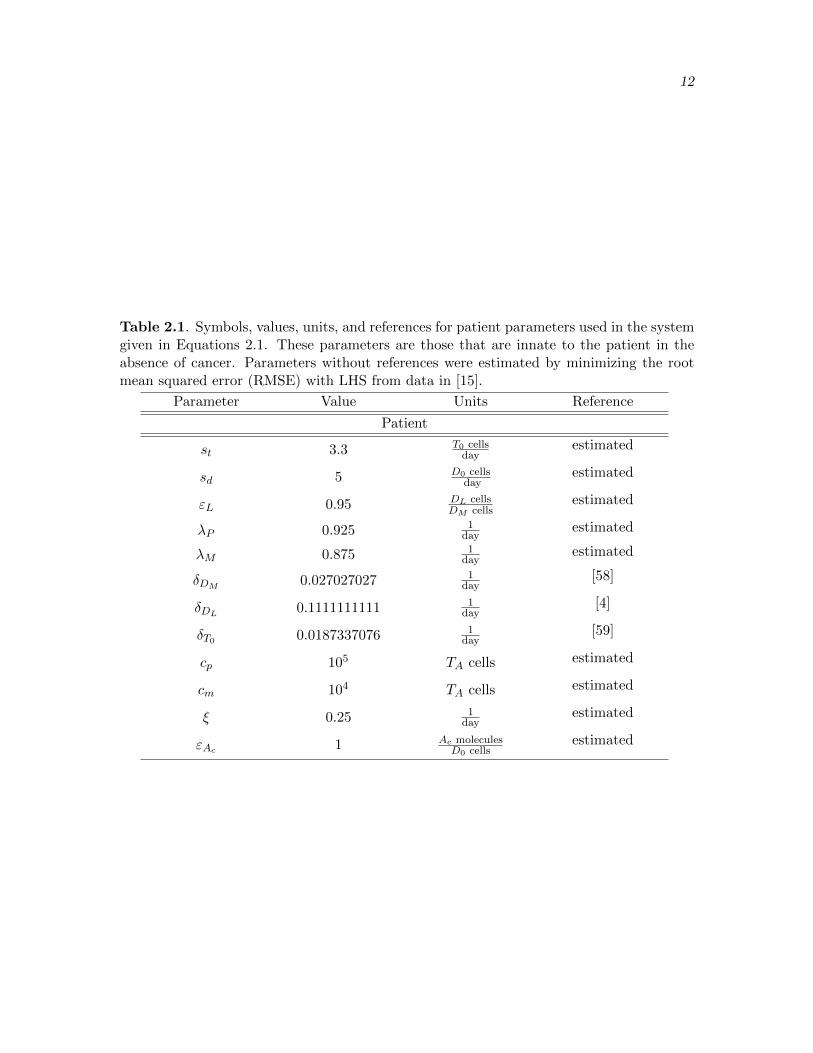
Table 2.1. Symbols, values, units, and references for patient parameters used in the systemgiven in Equations 2.1. These parameters are those that are innate to the patient in theabsence of cancer. Parameters without references were estimated by minimizing the rootmean squared error (RMSE) with LHS from data in [15].

Parameter Value Units Reference

Patient

st 3.3 T0 cellsday

estimated

sd 5 D0 cellsday

estimated

εL 0.95 DL cellsDM cells

estimated

λP 0.925 1day

estimated

λM 0.875 1day

estimated

δDM0.027027027 1

day[58]

δDL0.1111111111 1

day[4]

δT0 0.0187337076 1day

[59]

cp 105 TA cells estimated

cm 104 TA cells estimated

ξ 0.25 1day

estimated

εAc 1 Ac moleculesD0 cells

estimated

13

Table 2.2. Symbols, values, units, and references for regulatory T cell, cancer, and glycatedchitosan parameters used in the system given in Equations 2.1. Treg dynamics, cancerdynamics, and GC dynamics. Parameters without references were estimated by minimizingthe root mean squared error (RMSE) with LHS from data in [15].

Parameter Value Units Reference

Cancer

γP 0.63 1day

estimated

γM 0.2 1day

estimated

µ 0.008 1day

estimated

σ 0.45 M cellsP cell

estimated

ρ 100 Ac moleculesP cell · day

estimated

p 1 Ac moleculestumor cell

estimated

ω 1 1day

estimated

Treg

k 4.163995 unitless none

δD0 0.027027027 1day

[58]

εA 3 TA cellsTn cell

[60]

εi 3 Ti cellsTi−1 cell

[60]

η 0.9 1day

[4]

Glycated Chitosan

α 0.012 1Molecule · day

estimated

β 0.0183622094883075 1DL cell · day

estimated

εM 0.95 DM cellsD0 cell

estimated

η 0.9 1day

[4]

µ 0.008 1day

estimated

CHAPTER 3

ANALYSIS OF MATHEMATICAL MODEL

In order to understand the intricate details of anti-tumor laser immunotherapy as

described in [11, 12, 13, 14, 15, 16, 17, 18, 56], the following questions must be answered.

1. What is the baseline growth pattern for the DMBA-4 metastatic mammary tumor cell

line used in animal model studies for anti-tumor laser immunotherapy?

2. To link mathematical modeling results to animal model experimental data, can we

classify model dynamics and relate results to animal model data?

(a) What are the qualitative and quantitative properties of what would be considered

successful or failed treatment?

(b) In performing sensitivity analysis with parameters, what does the model predict

about the diversity of treatment outcomes?

(c) What features of anti-tumor laser immunotherapy can be modified and what impact

would these changes have on treatment outcome or post-treatment dynamics?

3. What is the role of GC in the development and dynamics of the immune response?

(a) How does GC affect tumor-immune dynamics after laser treatment, and how can

these effects be captured by and studied with a mathematical model?

(b) What model parameters could be changed to study the effects of varying levels of

glycated chitosan effectivity?

4. The importance of Treg suppression on immunotherapy outcome has been demonstrated

experimentally. Which modeled components are influenced by Treg regulation and would

benefit from Treg suppression?

(a) Since the model does not explicitly include Tregs, how can their effects be modeled

implicitly by changing key parameters that correspond to levels of Treg immuno-

suppressive activity?

(b) Can the model be used to link a patient’s clinical outcome with a given level of

Treg immunosuppressive activity?

15

3.1 Sensitivity Analysis

In order to more comprehensively explore the post-treatment dynamics that the model

predicts, it is necessary to solve the model for a considerably large number of different

parameter sets. It is desirable to minimize the number of parameter sets that must be

sampled to develop an overall concept of the model’s behavior. We also sample parameters

within a pre-defined range to adhere to as many biologically known parameters as possible.

To accomplish these goals, a method called Latin Hypercube Sampling (LHS) is used to

randomly generate 1000 different parameter sets [61].

3.1.1 Latin Hypercube Sampling

For LHS, each parameter is considered a random variable with some probability distribu-

tion function [62, 61]. Each parameter distribution is then divided into n intervals of equal

probability from which values are selected without replacement [62, 61] (see Figure 3.1).

Thus, if there are k parameters and one desires to sample n values for each parameter from

its distribution, then the final result will be an n× k matrix of n generated values for each

of the k parameters.

The LHS method provides efficient approximation of each probability distribution func-

tion due to the fact that it allows only a single value to be randomly selected in any one

interval of the n-interval subdivision of the parameter probability distribution function

[62, 61]. The random nature of this selection technique also ensures that a large portion

of the parameter space is sampled [62]. LHS is superior to simple random sampling of

parameters, with the assumption of some probability distribution function for a given

parameter, due to more efficient and broad exploration of each parameter space [62, 61]

Subdivided Parameter Distribution

1 2 . . . n

0 1

0

1

Figure 3.1. Example of howthe uniform distribution for eachparameter is divided into equallyprobable intervals from which sam-pling will take place without re-placement. Sampling the uniformdistribution with equally probableintervals implies that the intervalsare all of the same length. Assum-ing a different distribution wouldlead to unequal intervals to ensureequally probable selection.

16

●

●

●

●

●

●

●

●

●●

●

●

●

●

●

●

●

●

●●

●

●

●

●●

●

●

●●

●

●

●

●

●

●

●●

●●

●

●

●

●

●

●

●●

●

●

●

0.0 0.2 0.4 0.6 0.8 1.0

0.0

0.2

0.4

0.6

0.8

1.0

Random LHS With Marginal Distributions

●

●

●

●

●

●

●

●

●

●

●

●●

●

●

●

●

●

●

● ●

●

●

●

●

●

●●

●

●

●

●

●

●

●

●

●

●

●

●

●

●

●

●

●

●

●●

●

●

0.0 0.2 0.4 0.6 0.8 1.0

0.0

0.2

0.4

0.6

0.8

1.0

SRS Uniform With Marginal Distributions

Figure 3.2. Scatterplot of 50 points in the unit plane sampled with (on left) random LHSand (on right) simple random sampling (SRS) of the uniform distribution on [0,1]. Marginaldistribution histograms above and to the right scatterplot show the efficiency of random LHSand SRS in estimating the uniform distribution on [0,1]. Based on this comparison betweenLHS and SRS, it is clear that LHS is a better approximation of the uniform distributionfor the 50 points.

(see Figure 3.2).

Implementation of the Latin Hypercube design for sampling model parameters was done

using the randomLHS(n, k) function in the R [63] ‘lhs’ package [64], where n is the number

of generated parameter sets and k is the number of parameters. With the randomLHS()

function, values for each parameter are selected randomly from the uniform distribution

on [0, 1]. We constrained parameter values since biological rates are not arbitrary, so we are

able to define a minimum (pMin) and a maximum (pMax) for each parameter. We choose

pMin and pMax to be a scaled multiple of the baseline parameter value. In the context

of analyzing model sensitivity to changes in parameter values, the assumption of a uniform

distribution for each parameter could be replaced by another distribution. However, the

qualitative outcomes of model simulation will be the same regardless of the distribution

since sampled parameters will be scaled to be between pMin and pMax.

Once all n sets of parameters have been randomly selected, the result is an n×k matrix

(Latin Hypercube) where the ijth entry is the ith selection of the jth parameter. After the

n× k matrix is generated, parameters must be scaled so that they remain confined to our

pre-defined range. Transformation is calculated by

17

pGen = pGen(pMax− pMin) + pMin

where pGen is one of the generated parameter values in the n×k matrix with corresponding

maximum and minimum values pMax and pMin. Since the parameter distribution is

defined to be uniform on [0, 1], the maximum value that pGen can have is 1. If this is the

case, then the above formula reduces to

pGen = pMax

where pGen is the given maximal value within its pre-defined range. Similarly, the minimum

value pGen can have is 0. If this is the case, then the rescaling formula becomes

pGen = pMin

where pGen is the given minimal value within its pre-defined range. After all entries in the

n×k matrix have been rescaled, the result is a new n×k matrix with n randomly generated

values for all k parameters such that each value is within its allowable range [pMin, pMax].

3.2 Predictions of Treatment Outcomes

Treatments are typically performed 10 - 15 days after approximately 105 viable DMBA-4

metastatic mammary tumor cells are injected into each rat [12, 13, 14, 15, 16, 17, 18].

Tumors are injected with a solution composed of a photosensitizing agent called indocyanine

green and the immunoadjuvant glycated chitosan, and then irradiated for about 10 minutes

[12, 13, 14, 15, 16, 17, 18]. Post-treatment, the primary tumor continues to grow until it

reaches a peak in a range of 30 - 50 days following treatment [12, 13, 14, 15, 16, 17, 18].

Once a global peak has been reached for primary tumor burden, tumors begin to shrink in

size to eventual depletion within 100 days after treatment [12, 13, 14, 15, 16, 17, 18]. Since

tumor burden of treated rats in these experiments exhibits exponential growth and decay,

the mathematical model takes this into account using the simple exponential population

growth model.

The model produces the general case of successful treatment outlined above with data

from [15]. The model simulation of the general treatment dynamics for tumor burden

shown in [12, 13, 14, 15, 16, 17, 18], as well as the associated immune system dynamics

predicted by the model is shown in Figure 3.3. Model solutions were found using lsoda()

function in the R ‘deSolve’ package [65]. Using LHS of patient parameters, 1000 parameter

sets were generated. The model was solved for each parameter set, and the solution that

18

Time (days)

●●

●● ●●● ●●

●●

●

100

103

106

109

0 20 40 60 80 100

Tum

or (

cells

)

Primary Tumor (P) Metastatic Tumor (M)

Time (days)

100

103

106

109

1012

0 20 40 60 80 100A

ntig

en (

mol

ecul

es)

Antigen (Ac)

0 20 40 60 80 100

0

100

200

300

400

Time (days)

DC

s (c

ells

)

Naive Dendritic (D0) Migrating Dendritic (Dm) Lymphatic Dendritic (DL)

Time (days)

100

103

106

109

1012

0 20 40 60 80 100

CT

Ls (

cells

)

Naive T Cells (T0) Sum Prol. T Cells (T1 − Tn) Killing CTLs (TA)

Figure 3.3. Reproduced from Figure 2.2 in Section 2.1. Predicted tumor-immune dynamicsdemonstrating the general case of successful treatment. Primary and metastatic tumorburden data from [15]. In the upper left plot, closed black dots are primary tumor burdenexperimental data and open triangles are metastatic tumor burden experimental data. Solidand dashed curves in each plot are model simulations. Vertical dashed line in each plotrepresents the time of laser treatment at t = 10 days. In the lower right plot, CTL dynamicsare shown for n = 8 proliferative stages. The orange curve in the lower right plot is thetotal number of proliferating CTLs (i.e.

∑ni=1 Ti(t)).

19

minimized the root mean squared error was chosen to produce Figure 3.3. The data chosen

for comparison is in [15]. The upper left-hand plot in Figure 3.3 shows model simulation for

primary and metastatic tumor burdens with tumor burden data for each tumor type. The

tumor burden simulation reflects experimental observations since the tumor burden curves

increase to a peak between days 20 and 40, and then gradually decay to zero by the end of

the simulated period. This figure also shows the dynamics of tumor antigens. The model

simulation shows that there is an abrupt increase due to laser treatment and CTL-mediated

tumor cell killing. Antigen is slowly cleared as the tumor burden curves decay to zero.

In the lower left plot of Figure 3.3, dendritic cell dynamics are shown. The simulation

shows an initially existing population of naive dendritic cells that quickly decays due to laser

treatment at t = 10 days. These naive cells quickly become migratory cells, which then

become lymphatic dendritic cells. The solid black curve in the dendritic cell plot represents

the number of lymphatic dendritic cells. Since the tumor burden curves gradually decay

until the end of the treatment simulation, the lymphatic dendritic cell curve does not

significantly deviate from its maximum.

The lower right plot of Figure 3.3 shows model simulation for CTL dynamics. The

simulation shows an initially existing population of naive CTLs that quickly decays due

to lymphatic dendritic cell interaction. The solid red curve represents the total number

of actively killing CTLs after all of the proliferative stages have been completed. This

simulation shows the slight delay between CTL activation and the introduction of CTLs to

the tumor sites. Simulated curves for actively killing CTLs quickly increase to a maximum

between days 40 and 50, and then gradually decay until the end of the simulated period.

Model simulation of each proliferative CTL stage and the actively killing CTLs is shown

in Figure 3.4. The lowest curve (t ≥ 40) in this plot represents the first proliferative stage.

Each successively higher curve represents the ith proliferative stage (for i = 2, 3, . . . , 8). The

solid red curve represents the actively killing CTL population. This simulation comes from

the same solution as shown in Figure 3.3, where proliferative stages were summed to draw

focus on the active CTL stage.

In experimentally treated animals, there are several types of qualitative treatment out-

comes ranging from tumor clearance resulting in patient survival to tumor escape resulting

in the death of the patient [11, 12, 13, 14, 15, 16, 17, 18]. Based on the results of animal

experiments [11, 12, 13, 14, 15, 16, 17, 18], one of the following clinical outcomes is assigned

to each model simulation (see Figure 3.5):

20

Clearance - tumors are controlled quickly, primary tumor burden does not exceed 3×1010

cells, and primary tumor burden is below 100 cell by the end of the simulated study

period (solid green curves)

Slow Clearance - primary tumor burden clears slowly but not completely, there has not

been a relapse, and primary tumor burden does not exceed 3×1010 cells (dashed blue

curves)

Relapse - initial clearing of primary tumor burden with eventual re-growth to an obvious

peak, and primary tumor burden does not exceed 3×1010 cells (dotted purple curves)

Death - primary tumor burden exceeds 3×1010 cells and study animal is sacrificed (dashed

and dotted red curves)

It is known that different organisms within the same species routinely exhibit vastly

different immunities [4]. For the mathematical model, these immunological variances are

expressed by changes to model parameters. In line with the concept of random immune vari-

ability, 1000 different parameter sets were randomly generated by LHS. For each parameter

set, the model was solved with fixed initial conditions.

100

103

106

109

0 20 40 60 80 100

CT

Ls (

cells

)

Time (days)

Active CTLsStage 1Stage 2Stage 3Stage 4Stage 5Stage 6Stage 7Stage 8 Figure 3.4. Reproduced from

Figure 2.3 in Section 2.1. Pro-gression through the stages ofproliferation with the highestcurve (t ≥ 40) being the activeCTLs able to kill tumor cells.For t ≥ 40, the lowest curverepresents the first proliferativestage. Each successively highercurve represents the ith prolifer-ative stage for i = 2, 3, . . . , 8.

21

100

103

106

109

1012

1015

1018

1021

1024

0 20 40 60 80 100

Prim

ary

Tum

or (

cells

)

Time (days)

A. ClearanceSlow ClearanceRelapseDeath

100

103

106

109

1012

1015

1018

1021

1024

0 20 40 60 80 100

Met

asta

tic T

umor

(ce

lls)

Time (days)

B. ClearanceSlow ClearanceRelapseDeath

Figure 3.5. Model simulations produced as patient parameters vary about baseline param-eter set using LHS. All qualitatively different outcomes, as defined previously (Section 3.2),are represented. (A) Changes in primary tumor burden as patient parameters vary. (B)Changes in metastatic tumor burden as patient parameters vary.

3.3 Modeling the Effects of Glycated Chitosan (GC)

Immunoadjuvants are used to stimulate the immune system to achieve a more robust

immune response [66, 55]. In [11, 12, 13, 14, 15, 16, 17, 18, 56], the immunoadjuvant

glycated chitosan is used to stimulate the immune system in antitumor laser immunotherapy.

Immunoadjuvants have been shown to increase antigen uptake, aid in dendritic cell activa-

tion and maturation/migration, and aid in T cell activation [66, 55]. With the reasonable

assumption that glycated chitosan adopts a similar mode of immune stimulation, we can

model these effects by changing corresponding model parameters. Parameters that change

with varying levels of GC effectivity are:

• α - rate at which dendritic cells interact with antigen and become activated

• η - rate of dendritic cell migration

• εM - efficiency of naive to migratory dendritic cell conversion

• β - rate at which lymphatic dendritic cells interact with and activate naive CTLs

• µ - rate of primary tumor cell metastasis

Using LHS of GC parameters, 1000 different GC parameter sets were randomly gener-

ated. For each parameter set, the model was solved with fixed initial conditions to determine

22

model sensitivity to changes in GC levels. Simulations were qualitatively classified by

changes in overall tumor dynamics as outlined previously in Section 3.2.

Model sensitivity to changes in GC parameters is demonstrated in Figure 3.6. The

first column of this figure represents tumor burden dynamics for each outcome. The most

noticeable change from the effects of GC is shown in the second column, which represents

dendritic cell dynamics for varying degrees of GC effectivity. In the last row, the extremely

low number of DCs in the lymph nodes affects the eventual number of activated CTLs. This

in turn produces a tumor burden that is uncontrolled, which corresponds to patient death.

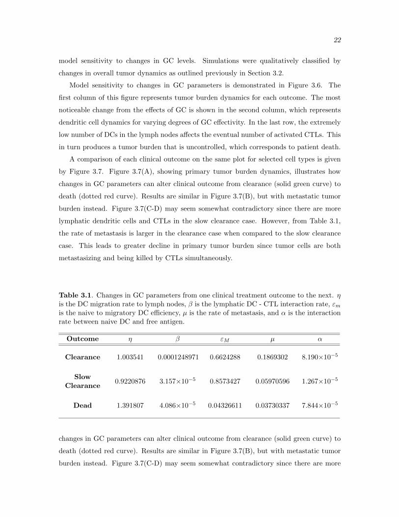
A comparison of each clinical outcome on the same plot for selected cell types is given

by Figure 3.7. Figure 3.7(A), showing primary tumor burden dynamics, illustrates how

changes in GC parameters can alter clinical outcome from clearance (solid green curve) to

death (dotted red curve). Results are similar in Figure 3.7(B), but with metastatic tumor

burden instead. Figure 3.7(C-D) may seem somewhat contradictory since there are more

lymphatic dendritic cells and CTLs in the slow clearance case. However, from Table 3.1,

the rate of metastasis is larger in the clearance case when compared to the slow clearance

case. This leads to greater decline in primary tumor burden since tumor cells are both

metastasizing and being killed by CTLs simultaneously.

Table 3.1. Changes in GC parameters from one clinical treatment outcome to the next. ηis the DC migration rate to lymph nodes, β is the lymphatic DC - CTL interaction rate, εmis the naive to migratory DC efficiency, µ is the rate of metastasis, and α is the interactionrate between naive DC and free antigen.

Outcome η β εM µ α

Clearance 1.003541 0.0001248971 0.6624288 0.1869302 8.190×10−5

SlowClearance

0.9220876 3.157×10−5 0.8573427 0.05970596 1.267×10−5

Dead 1.391807 4.086×10−5 0.04326611 0.03730337 7.844×10−5

changes in GC parameters can alter clinical outcome from clearance (solid green curve) to

death (dotted red curve). Results are similar in Figure 3.7(B), but with metastatic tumor

burden instead. Figure 3.7(C-D) may seem somewhat contradictory since there are more

23

lymphatic dendritic cells and CTLs in the slow clearance case. However, from Table 3.1,

the rate of metastasis is larger in the clearance case when compared to the slow clearance

case. This leads to greater decline in primary tumor burden since tumor cells are both

metastasizing and being killed by CTLs simultaneously.

100

103

106

109

1012

0 20 40 60 80 100

Tumor (cells)

Cle

aran

ce

PrimaryMetastatic

0 20 40 60 80 100

0

100

200

300

DCs (cells)

NaiveMigratoryLymphatic

100

103

106

109

0 20 40 60 80 100

CTLs (cells)

NaiveProliferatingKilling

100

103

106

109

1012

0 20 40 60 80 100

Slo

w C

lear

ance

PrimaryMetastatic

0 20 40 60 80 100

0

100

200

300

NaiveMigratoryLymphatic

100

103

106

109

0 20 40 60 80 100

NaiveProliferatingKilling

100

103

106

109

1012

0 20 40 60 80 100

Dea

th

Time (Days)

PrimaryMetastatic

0 20 40 60 80 100

0

100

200

300

Time (Days)

NaiveMigratoryLymphatic

100

103

106

109

0 20 40 60 80 100

Time (Days)

NaiveProliferatingKilling

Figure 3.6. For each clinical outcome (corresponding to rows) defined by tumor dynamics,simulations for each cell type are shown. Clinical outcome is highly correlated with themaintenance of CTLs throughout the simulated treatment. This indirectly indicates thatclinical outcome becomes more favorable as GC effectivity increases. Variation in GCparameters did not produce clinical outcome of tumor relapse.

24

100

103

106

109

1012

1015

0 20 40 60 80 100

Prim

. Tum

or (

cells

)A.

100

103

106

109

1012

1015

0 20 40 60 80 100

Met

a. T

umor

(ce

lls)

B.

0 20 40 60 80 100

0

50

100

150

200

250

Time (days)

Lym

ph. D

Cs

(cel

ls)

C.

Time (days)

100

103

106

0 20 40 60 80 100

CT

Ls (

cells

)D.

Clearance Slow Clearance Death

Figure 3.7. Depiction of changes in cellular dynamics as GC effectivity changes. In eachpanel, the clinical outcome of clearance (i.e., patient survival) is in solid green, the clinicaloutcome of slow clearance (prolonged survival) is in dashed blue curve, and the clinicaloutcome of death is in dotted red. Variation in GC parameters did not produce clinicaloutcome of tumor relapse.

3.4 Regulatory T Cell Experimental Simulation

Based on the immunosuppressive activity of regulatory T cells outlined in Section 1.6.3,

Treg effects can be modeled by their influence on corresponding model parameters. Param-

25

eters that change with varying levels of Treg activity are:

• δD0 - naive dendritic cell death rate (changes due to Tregs killing DCs)

• εA - proliferation constant for CTLs (changes due to Treg interference)

• k - death scaling constant for active CTLs (changes due to Tregs killing CTLs)

• η - migration rate for dendritic cells to lymph nodes (changes due to Treg interference).

Using LHS of Treg parameters, we randomly sampled 1000 different parameter sets

from each Treg parameter’s uniform distribution. Sampled parameters were then scaled to

a conservative range about each predefined baseline parameter value. The model was solved

for each parameter set with fixed initial conditions to produce results shown in Figures 3.8

and 3.9, which are classified according to overall tumor burden dynamics outlined previously

in Section 3.2.

The motivation for using LHS of Treg parameters primarily comes from the desire to

efficiently explore the Treg parameter space. The interpretation of the hypercube matrix

output is that each row corresponds to a unique level of Treg effectivity. The uniqueness

comes from the fact that each row contains no identical entries to any other row. This

is highly representative of the random variability in each individual’s immune parameters.

However, since we desire to search a Treg parameter space with a much larger range than

would generally be attributed to natural individual variation, we may also interpret each

row of the hypercube matrix to represent the effects of various immunosuppressive drugs

on Treg activity.

We interpreted the hypercube generated with Treg parameters as a combination of

1000 different patients undergoing immunotherapy treatment with the aid of some kind

of immunosuppressive drug inhibiting Treg activity. As shown in Figure 3.8, the model

simulations have sufficient variability to be partitioned with each of our clinical treatment

outcome definitions. The first column of Figure 3.8 represents the change in tumor burden

dynamics as Treg effectivity increases from top to bottom (primary-solid blue and metastatic

dashed-red). In the second column, the most obvious variability exists in the lymphatic

dendritic cell population (solid-black). In the best case (clearance), lymphatic dendritic

cells saturate the lymph nodes for the majority of the simulated study period.

Ultimately, clinical treatment outcome appears to be most strongly correlated with

CTL dynamics shown in the third column. There is an obvious decline in active CTL load

(solid-red) from top to bottom. An important thing to note is that active CTL load is much

26

100

103

106

109

1012

0 20 40 60 80 100

Tumor (cells)C

lear

ance

PrimaryMetastatic

0 20 40 60 80 100

0

100

200

300

DCs (cells)NaiveMigratoryLymphatic

100

103

106

109

1012

0 20 40 60 80 100

CTLs (cells)NaiveProliferatingKilling

100

103

106

109

1012

0 20 40 60 80 100

Slo

w C

lear

ance

PrimaryMetastatic

0 20 40 60 80 100

0

100

200

300

NaiveMigratoryLymphatic

100

103

106

109

1012

0 20 40 60 80 100

NaiveProliferatingKilling

100

103

106

109

1012

0 20 40 60 80 100

Rel

apse

PrimaryMetastatic

0 20 40 60 80 100

0

100

200

300

NaiveMigratoryLymphatic

100

103

106

109

1012

0 20 40 60 80 100

NaiveProliferatingKilling

100

103

106

109

1012

0 20 40 60 80 100

Dea

th

Time (Days)

PrimaryMetastatic

0 20 40 60 80 100

0

100

200

300

Time (Days)

NaiveMigratoryLymphatic

100

103

106

109

1012

0 20 40 60 80 100Time (Days)

NaiveProliferatingKilling

Figure 3.8. For each clinical outcome (corresponding to figure rows) defined by tumordynamics, simulations for each cell type are shown. This figure demonstrates how clinicaloutcome is highly correlated with the maintenance of CTLs throughout the simulatedtreatment. This indirectly indicates that clinical outcome becomes more favorable as Tregsbecome less effective in killing CTLs. Horizontal axes represent time in days.

27

lower than proliferative stage CTL load (dashed-orange). This is an indication that Tregs

are either killing active CTLs most efficiently or interfering with proliferation in the last

row of Figure 3.8. Dynamics of all cells are driven by the complex combination of all Treg

activities, which can be accounted for with changes to Treg parameters (δD0 , k, εA, and η).

100

103

106

109

1012

1015

0 20 40 60 80 100

Prim

. Tum

or (

cells

)

A.

100

103

106

109

1012

1015

0 20 40 60 80 100

Met

a. T

umor

(ce

lls)

B.

0 20 40 60 80 100

0

50

100

150

200

Time (days)

Lym

ph. D

Cs

(cel

ls)

C.

Time (days)

100

103

106

109

0 20 40 60 80 100

CT

Ls (

cells

)

D.

Clearance Slow Clearance Relapse Death

Figure 3.9. Depiction of changes in cellular dynamics as Treg activity changes. In eachpanel, the clinical outcome of clearance (i.e., patient survival) is in solid green, the clinicaloutcome of slow clearance (prolonged survival) is in dashed blue curve, the clinical outcomeof relapse (possible prolonged survival) is in dotted purple, and the clinical outcome of deathis in dotted-dashed red.

Figure 3.9 shows each clinical outcome for selected cells on the same plot. Primary tumor

dynamics are given in Figure 3.9(A) with the clearance (solid green), slow clearance (dashed

28

blue), relapse (dotted purple), and death (dashed and dotted red). Results are similar in

Figure 3.9(B), but represent metastatic tumor dynamics instead. As stated previously in

the discussion of Figure 3.8, the dendritic cell populations do not exhibit a large degree

of sensitivity to Treg parameters. This conclusion is supported by Figure 3.9(C), which

shows very little variation in lymphatic DC dynamics. The strongest correlation between

the tumor dynamics, as they are clinically defined, and immune dynamics comes from

Figure 3.9(D). Clearance, the ideal clinical outcome, is correlated with the highest CTL

load (solid green curve). As Treg effectivity increases, CTL load decreases and tumor

dynamics reflect less favorable clinical outcomes.

Based on Table 3.2, the outcomes shown in Figure 3.8 and Figure 3.9 are understandable.

Naive dendritic cell death increases from clearance to death, CTL fatalities increase from

clearance to death, and CTL proliferation decreases from clearance to death. Dendritic cell

migration does not follow an intuitive trend since the relapse and death cases occur with the

highest migration rates. However, this simply reflects the model’s negligible sensitivity to

changes in dendritic cell migration rates in comparison to changes in proliferation or death

rates for CTLs.

Table 3.2. Changes in Treg parameters from one clinical treatment outcome to the next.δD0 is the naive DC death rate, k is the active CTL death constant, η is the migratory ratefor migrating DCs, and εA is the proliferation factor of CTLs.

Outcome δD0 k η εA

Clearance 0.006218062 1.817664 2.954493 4.052652

SlowClearance

0.006218062 4.490838 1.10697 3.138794

Relapse 0.02390397 9.126924 3.046669 3.047921

Dead 0.02635106 6.259964 3.412577 2.251934

CHAPTER 4

DISCUSSION

4.1 Summary

The interactions between dendritic cells, the complete T cell repertoire, and antibodies

with cancerous tumor cells and their antigens has been modeled as a system of first order

ordinary differential equations [67, 68]. However, the overall treatment/post-treatment

dynamics can be captured by explicitly modeling only laser treatment, DCs, the cytotoxic

T cell subset, primary and metastatic tumor cells, and tumor antigen (see Equations 2.1

and B.1).

Ultimately, in this thesis we neglected explicit treatment of helper T cells, B cells,

and antibodies while achieving similar tumor dynamics. We justify the omission of such

immune components based on the fact that CTL effectivity is partially a function of

the activity of helper T cells and B cells. This means that a reparameterization of our

reduced-equation model (Equations 2.1) accounts for the effects of helper T cells and B

cells. This allows for a significant reduction in the number of unknown model parameters

and allows us to experiment with the effects of implicitly modeled components through

strategic reparameterization.

Analysis presented in Chapter 3 suggests that anti-tumor laser immunotherapy can be

accurately simulated with models like those presented in Chapter 2. As shown in Figure 3.3,

the model is capable of simulating post-treatment tumor dynamics similar to those seen

experimentally [15]. Because the model parameters are biologically realistic, the model can

be used for clinical treatment outcome predictions.

Systematically studying the effects of glycated chitosan and regulatory T cells with

LHS leads to diverse changes in tumor burden dynamics. The clinical outcome definitions

outlined in Chapter 3 allowed for partitioning of model simulations as a function of GC and

Treg parameters. It is important to make clinical outcome definitions to determine how

successful treatment will be for any given set of parameters or initial conditions.

30

Treg analysis suggests that a drug used for Treg suppression needs to primarily inhibit

their ability to affect CTL death and proliferation, because clinical outcomes correlate most

strongly with changes in CTL load over the course of the simulated study period (Figure 3.8).

Treg effects on dendritic cells in model simulations suggest a more complex relationship

between clinical outcome and DC dynamics; there is not a large degree of variability in DC

dynamics between the outcome cases. GC analysis suggests that clinical outcomes may be

less sensitive to changes in GC parameters than in the case for Treg parameters. However,

tumor dynamics still exhibit enough variability to partition simulations with three of the

defined clinical outcomes (Figure 3.6).

4.2 Suggested experiments

The analysis of anti-tumor laser immunotherapy from a modeling perspective suggests

a variety of experimental treatments to be performed in the laboratory. The following list

discusses a few experiments that might be useful in improving treatment efficacy.

1. Since it is possible to extract CTLs for the purpose of priming for a particular invader,

one suggestion would be to pursue this possibility alongside laser treatment. The goal

would be to train CTLs to attack the treated tumor cell line and build a substantial

CTL load for injection into the patient. The motivation comes from the fact that early

tumor infiltration is best in order to eradicate tumors. An injected population could

theoretically begin attacking primary and metastatic tumors soon after treatment before

a second line of activated CTLs arrives. This theory is supported by results found in

Section 3.2 (Figure 3.5).

2. Train dendritic cells before re-injecting them. The ultimate goal would be to activate as

many CTLs as possible, which might be enhanced through a larger number of primed

dendritic cells (Figure 3.5).

3. The timing of treatment tends to be crucial to patients with aggressively growing tumors.

Typically, treatments in anti-tumor laser immunotherapy are performed 7 to 10 days

post-inoculation. A possible experiment might be to wait a longer period of time before

treatment so that treatment efficacy could be tested in a much later stage of tumor

development.

4. Since tumor dynamics seem to be most closely tied to changes in Treg parameters, it

might be beneficial to try to derive a drug that either decreases the number of Tregs or

31

mitigates their ability to kill CTLs or affect CTL proliferation. The latter drug effect is

supported by Treg analysis in Section 3.4 (Figures 3.8 and 3.9).

CHAPTER 5

FUTURE WORK

5.1 Modeling

Many tumors exhibit growth patterns that cannot be explained with a simple exponen-

tial growth model. Exponential growth is used in the current model of anti-tumor laser

immunotherapy because the tumor burden data suggests this type of growth. However,

we can use the model to look at this treatment for other tumor cell lines. Some tumors

can be modeled with logistic growth, rP(1− P

K

). The logistic growth model includes

the assumption that there is some carrying capacity K that will affect overall population

dynamics. This carrying capacity is a type of ceiling for tumor growth, which is related to

nutrient availability and space. It would be quite simple to substitute a logistic term into

the primary and metastatic tumor equations to study other tumor types. The current model

can be used to study laser immunotherapy on any tumor cell line that exhibits exponential

growth. This would simply call for a reparameterization of the current model to account

for differences between tumor types.

The laser-tissue interaction in anti-tumor immunotherapy is much more complex than

the simple time-dependent treatment function used in the current model. In order to truly

understand primary tumor cell death as a function of laser heat, it is necessary to determine

how heat diffuses through a non-homogeneous tumor mass to produce cell death. This calls

for an application of the heat equation. The ability to quantify tumor cell death as a function

of heat shock would allow us to update the treatment function in the current model.

5.2 Experimentation

The model can easily be used to test experiments that are expensive to perform in the

laboratory setting. One such experiment would be to simulate the injection of a pre-primed

population of CTLs post-treatment to study how this would affect tumor dynamics. This

could be done by first solving the model until simulated injection was to take place and

33

then using the output as the initial conditions for post-injection dynamics. The CTL initial

condition would dramatically increase for the post-injection period. This could also be

done for dendritic cells by changing the initial condition for DCs after simulated injection

of pre-primed DCs.

As described in the previous section, the model could be reparameterized to study other

exponentially growing tumor lines undergoing laser immunotherapy. For tumors that reach

a carrying capacity well before the death of the patient, the logistic growth model might

be more accurate. With a minor change to the primary and metastatic tumor equations,

simulated laser immunotherapy treatment could be performed on tumors expected to exhibit

logistic growth.

5.3 Speculation

Based on the model’s sensitivity to changes in CTL dynamics, simulating the injection

of pre-primed CTLs would most likely yield a more successful treatment. Theoretically, this

should also be true if performed in the laboratory alongside anti-tumor laser immunotherapy.

Since the model is less sensitive to DC dynamics, one could surmise that clinical out-

comes would not be as sensitive to changes in DC populations by priming DCs outside

the patient. If GC primarily affects dendritic cells, this would indicate that changes in

GC administration should not have extreme implications for clinical treatment outcomes.

However, considering the comparison of clinical outcomes influenced by GC versus other

common adjuvants shown in [16], the effects of GC may be more complex than our current

understanding yields.

It may be most important to focus on methods to suppress Tregs due to the model’s

enhanced sensitivity to Treg parameters. If it is possible to suppress these cells in the tumor

microenvironment for an extended period of time, then the model suggests that CTLs will

be effective in tumor cell destruction.

APPENDIX A

IMMUNOLOGICALLY EXPANDED

MODEL

In our initial model, tumors were destroyed almost instantly with the chosen parameter-

ization. Based on the tumor burden data, this time course was not accurate. The proposed

mechanism behind the model on the next page is that antibody production is essential

to tumor cell destruction. This possible mechanism was suggested in [11], so we chose to

extend the model based on this hypothesis.

Since B cells produce antibodies upon activation, this required modeling three stages of

B cell development. However, activation of B cells requires stimulus by activated helper T

cells after B cells have received antigen via dendritic cells. Therefore, we modeled helper

T cells, B cells, and antibodies in order to account for a delay in tumor cell destruction.

Once tumors are tagged by selective antibodies, activated CTLs can then recognize them

for destruction. We also hypothesized that tumors may shed antibodies after some time, so

this introduced a small amount of feedback into the model. That is, tagged tumors could be

recycled back into the untagged tumor population and escape immune surveillance. This

meant that only sufficient antibody concentration would ultimately lead to a successful

treatment.

Upon further investigation of the antibody-induced tumor cell killing mechanism, we

could not reasonably conclude that this was the model that best fit the biology. This

divergence was based on several immunological facts that were previously unknown. One

of which, is fact that activated CTLs only need to be primed by a specific antigen in order

to effectively eradicate an invader. Evidence of this is given by studies in which CTLs

are extracted and trained to attack a specific tumor cell line and then re-injected, which

eventually leads to complete tumor destruction.

With new parameterization of the original model, we were able to accurately simulate

what is shown in tumor burden data. This allowed us to re-adopt a smaller model that is

35

computationally more manageable and biologically more accurate. As before, the function

φ(t) is a time-dependent treatment function that drives tumor death.

(Naive

Dendritic

) dD0

dt= sd − αAcD0 − δD0

D0(MigratoryDendritic

) dDM

dt= εMαAcD0 − ηDM − δDM

DM(LymphaticDendritic

) dDL

dt= εLηDM − k1(βT0 + bB0 + ψH0)DL − δLDL(

NaiveCTL

) dT0dt

= st − βDLT0 − δT0T0(

ActiveCTL

) dTAdt

= νtβDLT0 − k2δT0TA(

NaiveB Cell

) dB0

dt= sb − bB0DL − δB0B0(

StimulatedB Cell

) dBs

dt= εsbB0DL − τHABs − δBs

Bs(PlasmaB Cell

) dBp

dt= νbτHABs − δBp

Bp(IgG

Antibody

) dG

dt= zBp − δGG− θ(P0 +M0)G(

NaiveHelper T

) dH0

dt= sh − (ξBp + ψDL)H0 − δH0H0(

ActiveHelper T

) dHA

dt= νh(ξBp + ψDL)H0 − δHA

HA(UntaggedPrimary

) dP0

dt= (1− µ)γp(P0 + εxP1)− (φ(t) + θG+ λ0TA + δp)P0(

TaggedPrimary

) dP1

dt= (1− εx)(1− µ)γpP1 + εGθGP0 − (λ1TA + δp)P1(

UntaggedMetastatic

) dM0

dt= γm(M0 + εxM1) + σµγp(P0 + εxP1)− (θG+ λ0TA + δM )M0(

TaggedMetastatic

) dM1

dt= (1− εx)γmM1 + (1− εx)σµγpP1 + εGθGM0 − (λ1TA + δM )M1(

TumorAntigen

) dAc

dt= ρφ(t)P0 + pTA(λ0P0 + λ0M0 + λ1M1 + λ1P1)− (ω + αAc)D0

(A.1)

Excluding the antibody-mediated tumor cell destruction mechanism for post-treatment

dynamics, we can remove all B cell, helper T cell, and antibody related equations to

produce our initial model without CTL proliferation. This reduces the number of tumor

cell equations that we must track for post-treatment dynamics. Essentially, four tumor cell

equations in the expanded model become two equations in the reduced model.

APPENDIX B

REDUCED MODEL WITHOUT CTL

PROLIFERATION

With the reduced model without CTL proliferation, we have been able to accurately

predict clinical treatment outcomes as a function of GC and Treg effectivity. This model

has been very useful in that it has the capacity to explain a very complex system of events

taking place in anti-tumor immunotherapy, but it is also relatively small and easy to explain.

Interactions, in particular CTL-tumor cell interaction, are all modeled with mass-action

kinetics. However, CTL dynamics are not perfectly portrayed since overall numbers of

these cells are considerably low upon activation and tumor cell killing is simply too efficient.

Also, this model is quite stiff so solving can produce a large degree of numerical error. The

reduced model without proliferation is given as follows:

(Naive Dendr)dD0

dt= sd − αAcD0 − δD0D0

(Migratory Dendr)dDM

dt= εMαAcD0 − ηDM − δDM

DM

(Lymphatic Dendr)dDL

dt= εLηDM − δDL

DL

(Naive CTL)dT0dt

= st − βDLT0 − δT0T0

(Active CTL)dTAdt

= εAβDLT0 − kδT0TA

(Prim Tumor)dP

dt= γPP − (µ+ φ(t)− λPTA)P

(Meta Tumor)dM

dt= σµP + γMM − λMTAM

(Tumor Antigen)dAc

dt= ρφ(t)P + pTA(λPP + λMM)− ωAc − αAcD0

(B.1)

APPENDIX C

MODEL OF CTL PROLIFERATION

In order to model the delay in tumor cell destruction without arbitrarily changing

parameters to achieve this goal, we wrote the following proliferation model for CTLs upon

activation. The purpose of this was to simulate a more realistic number of CTLs after

activation and to accurately capture the time course of tumor - CTL interaction. Each

successive proliferative stage equation multiplies the addition from the previous proliferative

stage equation by some scaling factor εi in order to model cellular cloning from one stage

to the next. The end result is a large number of active CTLs that travels to the sites of

tumors and begins attacking them.

The proliferation equations given in Equations C.1:

(1st stage CTL)dT1dt

= ε1βDLT0 − ξT1 − δT0T1

(2nd stage CTL)dT2dt

= ε2ξT1 − ξT2 − δT0T2

(3rd stage CTL)dT3dt

= ε3ξT2 − ξT3 − δT0T3

(4th stage CTL)dT4dt

= ε4ξT3 − ξT4 − δT0T4

(5th stage CTL)dT5dt

= ε5ξT4 − ξT5 − δT0T5

(6th stage CTL)dT6dt

= ε6ξT5 − ξT6 − δT0T6

(7th stage CTL)dT7dt

= ε7ξT6 − ξT7 − δT0T7

(8th stage CTL)dT8dt

= ε8ξT7 − ξT8 − δT0T8

(Final stage CTL)dTAdt

= εAξT8 − kδT0TA

(C.1)

A comparison between CTL dynamics with and without proliferation is given in Fig-

ure C.1. Without proliferation, CTL killing of tumor cells must be extremely efficient

since the total number of CTLs at any given time is quite low. With the appropriate

38

parameterization and mass-action killing, we have modeled post-treatment tumor dynamics

accurately with our non-proliferation model. However, this model is not the most accurate

fit for the underlying immunology and can produce extensive numerical error when solving

the model. Figure C.1 is plotted on a log-scale, so the difference between CTLs with

proliferation vs. without is several orders of magnitude for the majority of the simulated

treatment period.

100

103

106

109

0 20 40 60 80 100

CT

Ls (

cells

)

Time (days)

Prol. CTLsNonProl. CTLs

Figure C.1. Comparison of CTL dynamics with proliferation (solid-red) and withoutproliferation (dashed-purple). Plot is on a log scale, so overall CTL loads differ by severalorders of magnitude as shown by vertical axis labels.

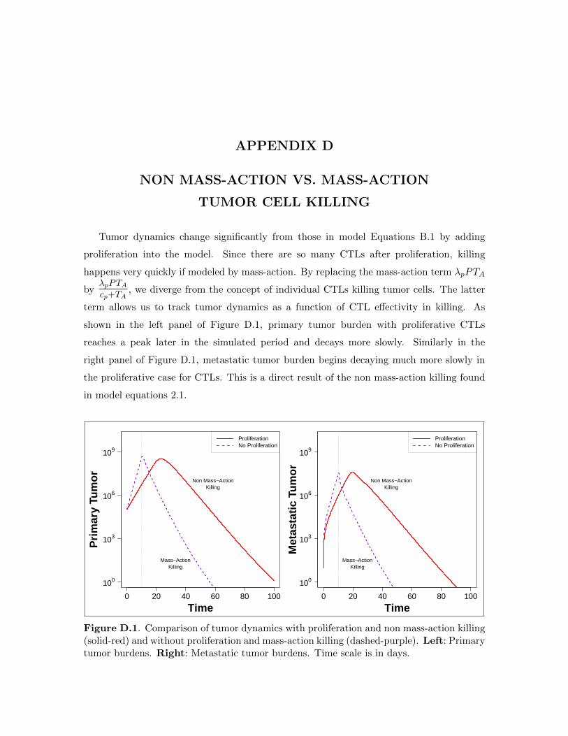
APPENDIX D

NON MASS-ACTION VS. MASS-ACTION

TUMOR CELL KILLING

Tumor dynamics change significantly from those in model Equations B.1 by adding

proliferation into the model. Since there are so many CTLs after proliferation, killing

happens very quickly if modeled by mass-action. By replacing the mass-action term λpPTA

byλpPTAcp+TA

, we diverge from the concept of individual CTLs killing tumor cells. The latter

term allows us to track tumor dynamics as a function of CTL effectivity in killing. As

shown in the left panel of Figure D.1, primary tumor burden with proliferative CTLs

reaches a peak later in the simulated period and decays more slowly. Similarly in the

right panel of Figure D.1, metastatic tumor burden begins decaying much more slowly in

the proliferative case for CTLs. This is a direct result of the non mass-action killing found

in model equations 2.1.

Time

100

103

106

109

0 20 40 60 80 100

Prim

ary

Tum

or

Mass−ActionKilling

Non Mass−ActionKilling

ProliferationNo Proliferation

Time

100

103

106

109

0 20 40 60 80 100

Met

asta

tic T

umor Non Mass−Action

Killing

Mass−ActionKilling

ProliferationNo Proliferation

Figure D.1. Comparison of tumor dynamics with proliferation and non mass-action killing(solid-red) and without proliferation and mass-action killing (dashed-purple). Left: Primarytumor burdens. Right: Metastatic tumor burdens. Time scale is in days.

REFERENCES

[1] Lauren Sompayrac. How Cancer Works. Jones and Bartlett Publishers, 2004.

[2] Douglas Hanahan and Robert A Weinberg. The hallmarks of cancer. Cell, 100(1):57– 70, 2000.

[3] Douglas Hanahan and Robert A. Weinberg. Hallmarks of cancer: The next generation.Cell, 144(5):646–674, 2016/05/04 2011.

[4] Lauren Sompayrac. How the Immune System Works. John Wiley & Sons, Ltd, 4edition, 2012.

[5] Steven A Rosenberg, James C Yang, and Nicholas P Restifo. Cancer immunotherapy:moving beyond current vaccines. Nat Med., 10(9):909–915, September 2004.

[6] Immunotherapy for Lung Cancer, volume 6 of Proceedings of the American ThoracicSociety, 2009.

[7] Timothy P Cripe, Pin-Yi Wang, Paola Marcato, Yonatan Y Mahller, and PatrickWK Lee. Targeting Cancer-Initiated Cells With Oncolytic Viruses. Molecular Therapy,17(10):1677–1682, October 2009.

[8] Han Hsi Wong, Nicholas R. Lemoine, and Yaohe Wang. Oncolytic Viruses for CancerTherapy: Overcoming the Obstacles. Viruses, 2:78–106, January 2010.

[9] Saleem Meerani and Yang Yao. Oncolytic Viruses in Cancer Therapy. EuropeanJournal of Scientific Research, 40(1), 2010.

[10] Sanja Stevanovic, Lindsey M. Draper, Michelle M. Langhan, Tracy E. Campbell,Mei Li Kwong, John R. Wunderlich, Mark E. Dudley, James C. Yang, RichardM. Sherry, Udai S. Kammula, Nicholas P. Restifo, Steven A. Rosenberg, and ChristianS. Hinrichs. Complete Regression of Metastatic Cervical Cancer After TreatmentWith Human Papillomavirus-Targeted Tumor-Infiltrating T Cells. JOURNAL OFCLINICAL ONCOLOGY, 2015.

[11] Wei R. Chen, Robert L. Adams, Raoul Carubelli, and Robert E. Nordquist. Laser-photosensitizer assisted immunotherapy: a novel modality for cancer treatment. Can-cer Letters, 115:25–30, 1997.

[12] Wei R. Chen, Wei-Guo Zhu, Joseph R. Dynlacht, Hong Liu, and Robert E. Nordquist.Long-Term Tumor Resistance Induced by Laser Photo-Immunotherapy. Int. J. Cancer,81:808–812, 1999.

[13] Wei R. Chen, Anil K. Singhal, Hong Liu, and Robert E. Nordquist. AntitumorImmunity Induced by Laser Immunotherapy and Its Adoptive Transfer. CancerResearch, 61:459–461, 2001.

41

[14] Wei R. Chen, Hong Liu, Jerry W. Ritchey, Kenneth E. Bartels, Michael D. Lucroy,and Robert E. Nordquist. Effect of Different Components of Laser Immunotherapyin Treatment of Metastatic Tumors in Rats. Cancer Research, 62:4295–4299, August2002.

[15] Wei R. Chen, Sang Won Jeong, Michael D. Lucroy, Roman F. Wolf, Eric W. Howard,Hong Liu, and Robert E. Nordquist. Induced Antitumor Immunity Against DMBA-4Metastatic Mammary Tumors in Rats Using Laser Immunotherapy. Int. J. Cancer,107:1053–1057, 2003.

[16] Wei R. Chen, Mladen Korbelik, Kenneth E. Bartels, Hong Liu, Jinghai Sun, andRobert E. Nordquist. Enhancement of Laser Cancer Treatment by a Chitosan-DerivedImmonoadjuvant. Photochemistry and Photobiology, 81:190–195, 2005.

[17] M. F. Naylor, W.R. Chen, T.K. Teague, L.A. Perry, and R.E. Nordquist. In situphotoimmunotherapy: a tumour-directed treatment for melanoma. British Journal ofDermatology, 155:1287–1292, 2006.

[18] Sheng Song, Feifan Zhou, Robert E. Nordquist, Raoul Carubelli, Hong Liu, and Wei R.Chen. Glycated chitosan as a new non-toxic immunological stimulant. Immunophar-macology and Immunotoxicology, 31:202–208, 2009.

[19] Kathleen P. Wilkie and Philip Hahnfeldt. Tumor-Immune Dynamics Regulate in theMicroenvironment Inform the Transient Nature of Immune-Induced Tumor Dormancy.Cancer Research, 73:3534–3544, March 2013.

[20] Mustafa Mamat, Subiyanto Kartono, and Agus Kartono. Mathematical Model of Can-cer Treatments Using Immunotherapy, Chemotherapy and Biochemotherapy. AppliedMathematical Sciences, 7(5):247–261, 2013.

[21] Natalie Kronik, Yuri Kogan, Moran Elishmereni, Karin Halevi Tobias, Stanimir VukPavlovic, and Zvia Agur. Predicting Outcomes of Prostate Cancer Immunotherapy byPersonalized Mathematical Models. PLoS ONE, 5(12), December 2010.

[22] Artem S Novozhilov, Faina S Berezovskaya, Eugene V Koonin, and Georgy P Karev.Mathematical modeling of tumor therapy with oncolytic viruses: Regimes with com-plete tumor elimination within the framework of deterministic models. Biology Direct,1(6), February 2006.

[23] Ralph M. Steinman. The Dendritic Cell System and Its Role in Immunogenicity.Annual Review of Immunology, 9:271–296, 1991.

[24] Ralph M. Steinman and Joel Swanson. The Endocytic Activity of Dendritic Cells. J.Exp. Med., 182:283–288, August 1995.

[25] Federica Sallusto, Marina Cella, Carlo Danieli, and Antonio Lanzavecchia. DendriticCells Use Macropinocytosis and the Mannose Receptor to Concentrate Macromoleculesin the Major Histocompatibility Complex Class II Compartment: Downregulation byCytokines and Bacterial Products. J. Exp. Med., 182:389–400, August 1995.

[26] Ralph M. Steinman, Kayo Inaba, Shannon Turley, Philippe Pierre, and Ira Mellman.Antigen Capture, Processing, and Presentation by Dendritic Cells: Recent Cell Bio-logical Studies. Human Immunology, 60:562–567, January 1999.

42

[27] Peter Thumann, Isabelle Moc, Jens Humrich, Thomas G. Berger, Erwin S. Schultz,Gerold Schuler, and Lars Jenne. Antigen Loading of dendritic cells with whole tumorcell preparations. Journal of Immunological Methods, 277:1–16, February 2003.

[28] Theresa L. Whiteside, Joanna Stanson, Michael R. Shurin, and Soldano Ferrone.Antigen-Processing Machinery in Human Dendritic Cells: Up-Regulation by Matu-ration and Down-Regulation by Tumor Cells. The Journal of Immunology, 173:1526–1534, 2004.

[29] Brenda Gonzalez, Carlos Guerra, Devin Morris, Dennis Gray, and Vishwanath Ven-keteraman. Dendritic cells in infectious disease, hypersensitivity, and autoimmu-nity. International Journal of Interferon, Cytokine and Mediator Research, 2:137–147,November 2010.

[30] Xiaosong Li, Tomas Hode, Maria C. Guerra, Gabriela L. Ferrel, Robert E. Nordquist,and Wei R. Chen. Laser immunotherapy for treatment of patients with advanced breastcancer and melanoma. Journal of Physics, 2010.

[31] Arun T. Kamath, Sandrine Henri, Frank Battye, David F. Tough, and Ken Shortman.Developmental kinetics and lifespan of dendritic cells in mouse lymphoid organs.Immunobiology, 100(5):1734–1741, April 2002.

[32] Miriam Merad and Markus G. Manz. Dendritic cell homeostasis. Blood, 113(15):3418–3427, April 2009.

[33] Xinyuan Chen, Qiyan Zeng, and Mei X. Wu. Improved efficacy of dendritic cell-basedimmunotherapy by cutaneous laser illumination. Clinical Cancer Research, 18(8):2240–2249, April 2012.

[34] Karolina Palucka and Jacques Banchereau. Cancer immunotherapy via dendritic cells.Nature Reviews Cancer, 12:265–277, April 2012.

[35] Michio Tomura, Akihiro Hata, Satoshi Matsucka, Francis H. W. Shand, YasutakaNakanishi, Ryoyo Ikebuchi, Satoshi Ueha, Hidekazu Tsutsui, Kayo Inaba, KoujiMatsushima, Atsushi Miyawaki, Kenji Kabashima, Takeshi Watanabe, and OsamiKanagawa. Tracking and quantification of Dendritic cell migration and antigentrafficking between the skin and lymph nodes. Scientific Reports, 4(6030):1–11, August2014.

[36] Max Schnurr, Qiyuan Chen, Amanda Shin, Weisan Chen, Tracey Toy, Corinna Jen-derek, Simon Green, Lena Miloradovic, Debbie Drane, Ian D. Davis, Jose Villadangos,Ken Shortman, Eugene Maraskovsky, and Jonathan Cebon. Tumor antigen processingand presentation depend critically on dendritic cell type and the mode of antigendelivery. Immunobiology, 105(6):2465–2472, March 2005.

[37] Femke Broere, Sergei G. Apasov, Michail V. Sitkovsky, and Willem van Eden. Princi-ples of Immunopharmacology. Springer, 3rd edition, 2011.

[38] Sine Hadrup, Marco Donia, and Per thor Straten. Effector CD4 and CD8 T Cells andTheir Role in the Tumor Microenvironment. Cancer Microenvironment, 6:123–133,December 2012.

43

[39] Victor Appay, Rene A. W. can Lier, Federica Sallusto, and Mario Roederer. Phenotypeand Function of Human T Lymphocyte Subsets: Consensus and Issues. Cytometry,73A:975–983, September 2008.

[40] Nu Zhang and Michael J. Bevan. CD8+ T Cells: Foot Soldiers of the Immune System.Immunity, 35:162–168, August 2011.

[41] Bo Wang, Christopher C. Norbury, Roberta Greenwood, Jack R. Bennink, Jonathan W.Yewdell, and Jeffrey A. Frelinger. Multiple Paths for Activation of Naive CD8+ TCells: CD4-Independent Help. The Journal of Immunology, 167:1283–1289, 2001.

[42] Shimon Sakaguchi, Tomoyuki Yamaguchi, Takashi Nomura, and Masahiro Ono. Reg-ulatory T Cells and Immune Tolerance. Cell, 133:775–787, May 2008.

[43] William L. Byrne, Kingston H.G. Mills, James A. Lederer, and Gerald C. O’Sullivan.Targeting Regulatory T Cells in Cancer. Cancer Research, pages 6915–6920, November2011.

[44] Mark J Smyth, Shin Foong Ngiow, and Michele WL Teng. Targeting regulatory Tcells in tumor immunotherapy. Immunology and Cell Biology, 92:473–474, April 2014.

[45] Jinfang Zhu, Hidehiro Yamane, and William E. Paul. Differentiation of Effector CD4T Cell Populations. Annual Review of Immunology, 28:445–489, November 2010.

[46] Yo-Ping Lai, Chung-Jiuan Jeng, and Shu-Ching Chen. The Roles of CD4+ T Cells inTumor Immunity. International Scholarly Research Network, 2011:1–6, 2011.

[47] Ren E.M. Toes, Ferry Ossendorp, Rienk Offringa, and Cornelis J.M. Melief. CD4 TCells and Their Role in Antitumor Immune Responses. The Journal of ExperimentalMedicine, 189(5):753–756, March 1999.

[48] Kenneth Hung, Robert Hayashi, Anne Lafond-Walker, Charles Lowenstein, DrewPardoll, and Hyam Levitsky. The Central Role of CD4+ T Cells in the AntitumorImmune Response. J. Exp. Med., 188(12):2357–2368, December 1998.

[49] Yisong Y. Wan and Richard A. Flavell. How Diverse-CD4 Effector T Cells and theirFunctions. Journal of Molecular Cell Biology, 1:20–36, May 2009.

[50] Jinfang Zhu and William E. Paul. CD4 T cells: fates, functions, and faults. Blood,112(5):1557–1569, September 2008.

[51] Alvaro Lladser, Rolf Kiessling, and C. Christian Johansson. Regulatory T Cells inCancer. Cancer Research, 2010.

[52] Ulf Petrausch, Christian H. Poehlein, Shawn M. Jensen, Chris Twitty, James A.Thompson, Ilka Assmann, Sachin Puri, Michael G. LaCelle, Tarsem Moudgil, LeviMaston, Kevin Friedman, Sarah Church, Elisa Cardenas, Daniel P. Haley, Edwin B.Walker, Emmanuel Akporiaye, Andrew D. Weinberg, Sidney Rosenheim, Todd S.Crocenzi, Hong-Ming Hu, Brendan D. Curti, Walter J. Urba, and Bernard A. Fox.Cancer Immunotherapy: The Role Regulatory T Cells Play and What can be Done toOvercome Their Inhibitory Effects. Curr Mol Med., 9(6):673–682, August 2009.

44

[53] Feifan Zhou, Sheng Song, Wei R. Chen, and Da Xing. Immunostimulatory propertiesof glycated chitosan. Journal of X-Ray Science and Technology, 19:285–292, 2011.

[54] Assaf Marcus, Benjamin G. Gowen, Thornton W. Thompson, Alexandre Iannello,Michele Ardolino, Weiwen Deng, Lin Wang, Nataliya Shifrin, and David H. Raulet.Recognition of tumors by the innate immune system and natural killer cells. AdvImmunol., 122:91–128, 2014.

[55] Alberta Di Pasquale, Scott Preiss, Fernanda Tavares Da Silva, and Nathalie Garcon.Vaccine Adjuvants: from 1920 to 2015 and Beyond. Vaccines, 3:320–343, April 2015.

[56] Xiaosong Li, Min Min, Nan Du, Ying Gu, Tomas Hode, Mark Naylor, Dianjun Chen,Robert E. Nordquist, and Wei R. Chen. Chitin, Chitosan, and Glycated ChitosanRegulate Immune Responses: The Novel Adjuvants for Cancer Vaccine. Clinical andDevelopmental Immunology, 2013(387023), 2013.

[57] Anton Zilman, Vitaly V. Ganusov, and Alan S. Perelson. Stochastic Models ofLymphocyte Proliferation and Death. PLoS ONE, 5(9), September 2010.

[58] Isabelle Cremer, Marie-Caroline Dieu-Nosjean, Sylvie Marechal, Colette Dezutter-Dambuyant, Sarah Goddard, David Adams, Nathalie Winter, Christine Menetrier-Caux, Catherine Sautes-Fridman, Wolf H. Fridman, and Chris G. F. Mueller. Long-lived immature dendritic cells mediated by TRANCE-RANK interaction. Blood,100(10):3646–3654, November 2002.

[59] M. McDonagh and E. B. Bell. The survival and turnover of mature and immatureCD8 T cells. Immunology, 84, 1995.

[60] Kaja Murali-Krishna, John D. Altman, M. Suresh, David J. D. Sourdive, Allan J.Zajac, Joseph D. Miller, Jill Slansky, and Rafi Ahmed. Counting Antigen-Specific CD8T Cells: A Reevaluation of Bystander Activation During Viral Infection. Immunity,8:177–187, February 1998.

[61] M. D. McKay, R. J. Beckman, and W. J. Conover. A comparison of three methodsfor selecting values of input variables in the analysis of output from a computer code.Technometrics, 42(1):55–61, February 2000.

[62] S.M. Blower and H. Dowlatabadi. Sensitivity and Uncertainty Analysis of ComplexModels of Disease Transmission: an HIV Model, as an Example. InternationalStatistical Review, 62(2), 1994.

[63] R Core Team. R: A Language and Environment for Statistical Computing. RFoundation for Statistical Computing, Vienna, Austria, 2016.

[64] Rob Carnell. lhs: Latin Hypercube Samples, 2012. R package version 0.10.

[65] Karline Soetaert, Thomas Petzoldt, and R. Woodrow Setzer. Solving DifferentialEquations in R: Package deSolve, 2010.

[66] Teena Mohan, Priyanka Verma, and D. Nageswara Rao. Novel adjuvants & deliveryvehicles for vaccine development: A road ahead. Indian Journal of Medical Research,138(5):779–795, 2013.

45

[67] Sean M. Laverty, Bryan A. Dawkins, and Wei R. Chen. Laser immunotherapy and thetumor-immune system interaction: a mathematical model and analysis. Biophotonicsand Immune Responses IX, SPIE 8944(894409), February 2014.

[68] Bryan A. Dawkins and Sean M. Laverty. A mathematical model of the dynamicsof antitumor laser immunotherapy. Biophotonics and Immune Responses IX, SPIE8944(89440W), February 2014.