Embed Size (px)
Citation preview
Commun. Comput. Phys.doi: 10.4208/cicp.090412.121012a
Vol. 14, No. 2, pp. 477-508August 2013
Mathematical Modelling and Numerical Simulation
of Dendrite Growth Using Phase-Field Method with
a Magnetic Field Effect
A. Rasheed1 and A. Belmiloudi2,∗
1 COMSATS-IIT, Quaid Avenue, Wah Cantt, Pakistan.2 IRMAR-INSA de Rennes, 20 avenue des Buttes de Coesmes, CS 70839,35708 Rennes Cedex 7, France.
Received 9 April 2012; Accepted (in revised version) 12 October 2012
Available online 4 January 2013
Abstract. In this paper, we present a new model developed in order to analyze phe-nomena which arise in the solidification of binary mixtures using phase-field method,which incorporates the convection effects and the action of magnetic field. The modelconsists of flow, concentration, phase field and energy systems which are nonlinearevolutive and coupled systems. It represents the non-isothermal anisotropic solidi-fication process of a binary mixture together with the motion in a melt with the ap-plied magnetic field. To illustrate our model, numerical simulations of the influenceof magnetic-field on the evolution of dendrites during the solidification of the binarymixture of Nickel-Copper (Ni-Cu) are developed. The results demonstrate that thedendritic growth under the action of magnetic-field can be simulated by using ourmodel.
AMS subject classifications: 76W05, 35K55, 35R35, 74A50, 74N25, 65N30, 80A22
Key words: Modelling, Phase-field method, dendritic solidification, binary alloys, convection,magnetic-field, Magnetohydrodynamics, numerical simulations.
1 Introduction
In order to improve the quality and properties of mixtures, the major industrial chal-lenges lie in the possibility to control the metal structure and its defects, that occur duringthe solidification process and then to achieve the desired properties in the final solidifiedmetals.
∗Corresponding author. Email addresses: [email protected] (A. Rasheed),[email protected], [email protected] (A. Belmiloudi)
http://www.global-sci.com/ 477 c©2013 Global-Science Press
478 A. Rasheed and A. Belmiloudi / Commun. Comput. Phys., 14 (2013), pp. 477-508
In recent years the so-called phase field models have become an important tool tosimulate, during the solidification of pure and mixtures of materials, the formation andgrowth of dendrites. This approach has proved to be an emerging technology that com-plements experimental research. Various problems associated with phase-field formula-tion have been studied to treat both pure materials and binary alloys. From the theoreticalor numerical simulation point view, see e.g. A. Belmiloudi et al. [5–7], D. Kessler [15], P.Laurencot [17], J. Rappaz et al. [24], S. L. Wang et al. [33] and A. A. Wheeler et al. [36].We can note the existence of analytical solutions for this type of model, but it remainslimited to very simple cases. In the case of realistic situations where the system is highlynonlinear and very complex, the numerical simulation is a necessary tool, even essential,it plays an important role in understanding and analyzing the formation of microstruc-tures of dendrites. In this context, we can cite works of e.g., M. Grujicic et al. [10], B.Kaouil et al. [13], J. C Ramirez et al. [22, 23], M. Rappaz [25], T. Takaki et al. [29] and J.A. Warren et al. [34]. Moreover, in the last decade, the phase field method has been ex-tended to include the effect of convection on the dendrite growth. This was motivatedby the fact that during the solidification experiments it has been observed a meaningfulimpact of the movement in the liquid on the formation and evolution of the dendritic mi-crostructure. For phase-field models and the simulations of dendrite growth that includethe melt flow, we can cited e.g., in the case of phase-field models for the solidificationof a pure metal, D. M. Anderson et al. [2] that have developed a model in which theyintroduced the convection using compressible Navier-Stokes equations by assuming thatviscosity and density are the functions of phase-field in order to obtain the required vis-cosity and density variation between the two phases; R. Tonhardt et al. [31] and X. Tongal. [30] have given models by introducing convection using Navier-Stokes equations andenforcing the velocity to be zero in the solid phase. For other models which incorpo-rate convection during the solidification, we can cite N. Al-Rawahi et al. [1], E. Bansch etal. [3]. The principle obstacle in these simulations is to compute accurately the diffusionand convection processes and to enforce the no-slip condition at the interface so that thevelocity moves along-with the solid liquid interface during the solidification process.
Although significant advances in numerical simulation of microstructural evolutionin the metallurgical and materials science, and therefore it is now recognized that thanksto the phase field methods, we can simulate numerically the dendritic growth in the en-tire domain (at the macro scale level) with actual (physically meaningful) dimensions, itstill poses new and challenging problems for scientific community, because of the needto obtain approximate solutions more and more accurate and reliable. This goal can beachieved through the development of numerical analysis tools capable of reproducingfine qualitative properties and approximations of dendritic dynamics with a reasonableCPU’s computation time. To reach this objective, different approaches have been recentlydeveloped, we can cite e.g. H. Wang et al. [32] in which the authors provide an r-adaptivemoving mesh method for the quantitative phase field equations (which were providedby A. Karma et al. [14]), in both two- and three-dimensional cases. They redistribute themeshes in the physical domain by solving an optimization problem which automatically
A. Rasheed and A. Belmiloudi / Commun. Comput. Phys., 14 (2013), pp. 477-508 479
includes the boundary conditions and solve the mesh equations by using a multigridspeedup approach. In S. Bhattacharyya et al. [8], a spectral iterative-perturbation methodwas developed to compute the stress distribution in polycrystalline materials with arbi-trary elastic inhomogeneity and anisotropy in a multi-phase field model. For a reviewof the recent development of numerical methods for multi-component fluid flows withinterfacial phenomena in phase-field models see e.g. J. Kim [16].
However most of these simulations show that the dendrites are deformed consider-ably along the melt flow but the structure of dendrites can not be controlled using thesemethods. More recently, experiments have been made to control the metal structure andits defects that occur, because of the non-uniform dendrites in the final product, duringthe solidification process to improve the quality and properties of the metals by usingdifferent means. It has shown experimentally that the microstructure of mixtures can becontrolled during the solidification process by the application of magnetic field and elec-tric current (see, e.g., Mingjun Li et al. [18]). In particular, it has been proven by differentexperiments that the coarse dendrites in the solidified material can be made finer, homo-geneous and equiaxed to other dendrites by the application of magnetic field. For otherapplications of the influence of magnetic fields on the materials, we can cite, e.g., for theMHD flows H. B. Hadid et al. [12, 28], for the semi-conductor melt flow in the crystalgrowth A. Belmiloudi [7], M. Gunzberger et al. [11], M. Watanabe et al. [35], V. Galindoet al. [9] and for the solidification processes, J. K. Roplekar and J. A. Dantzig [26], P. J.Prescott [20] and the references therein.
To study the effect of convection and magnetic field on the evolution of micro-structureof dendrites, we have constructed a new phase-field model to simulate directional so-lidification and dendritic crystal growth that incorporate, among other, the convection,magnetic field and their interaction. The mathematical formulation of our model is com-posed of magnetohydrodynamic, concentration and phase-field systems which are time-dependent, non-linear and coupled systems in an isothermal environment. The com-mencing point of the present work is the two dimensional model of solidification of thebinary alloys given by Warren and Boettinger [34] (they have developed a phase-fieldmodel with the state variables phase-field parameter and relative concentration of themixtures). In order to take into account the topological changes of the micro-structureefficiently, we have included among other the effect of convection in the phase-field andsolute equations in the Warren-Boettinger model and also we have introduced the equa-tions of melt flow in the liquid phase in the presence of magnetic field which is applied ex-ternally to the entire domain. We can note that this new model, developed in the presentpaper, has been used in A. Belmiloudi and A. Rasheed [21] for the 2-dimensional isotropicand isothermal case. For this particular case, the existence and uniqueness results havebeen proved.
The paper is outlined as follows. Section 2 is concerned with the derivation of theequations governing the model. In Section 3 we give the adimensional quantities usedto non-dimensionalize the model and the initial conditions of the solidification process.We discuss the numerical resolution and implementation details of the problem, then
480 A. Rasheed and A. Belmiloudi / Commun. Comput. Phys., 14 (2013), pp. 477-508
we present numerical simulations of the dendrite growth of our model by consideringdifferent magnetic fields and compare the dendrites obtained in different simulations.Finally, conclusions are given in Section 4.
2 Mathematical modeling
2.1 Derivation of the model
Let Ω be a bounded, open, connected region of IRn, where n≤3 is the number of space di-mension, with a piecewise smooth boundary Γ=∂Ω which is sufficiently regular. Initiallythe region Ω is occupied by a binary alloy of the solute B (e.g., Cu) in the solvent A (e.g.,Ni), which is considered as incompressible electrically conducting fluid. To develop themodel, first we present the derivation of the flow systems, second we give the detaileddescription of phase-field equation and finally the concentration and energy equationswill be given.
Now we describe the flow equations. The evolution equations for the melt flow arederived from the laws of conservation of momentum and mass. The motion of the fluid isinitially driven by the buoyancy force. Since the fluid is electrically conducting and alsothere is an applied magnetic field B, therefore when the fluid starts moving there wouldbe electric current. In addition to the applied magnetic field B, there will be inducedmagnetic field produced by the electric currents in the liquid metal. Therefore there willbe Lorentz force which acts on the fluid so that an extra body force term F will appear inthe Navier-Stokes equations. The Lorentz force in such a flow is given by†
F=ρeE+J×B, (2.1)
where ρe is the electric charge density, E is the electric field intensity, J is the currentdensity and B is the applied magnetic field. We assume that the walls of the domainare electric insulators and the magnetic Reynolds number is sufficiently small that theinduced magnetic field is negligible as compared to the imposed magnetic field B. Thecurrent density J appeared in Eq. (2.1) can be defined by the Ohm’s law for the movingmedium as
J=ρeu+σe(E+u×B), (2.2)
where σe is electrical conductivity and u is the velocity of the fluid. As ρe is usually verysmall in liquid metals, therefore we shall neglect the terms ρeE and ρeu in Eqs. (2.1) and(2.2). Also as electric field is a conservative field, therefore we can express it as E=−∇φ,where ∇ is the gradient operator, φ is the potential function. Then the Lorentz force,given in (2.1), takes the form
F=σe (−∇φ×B+(u×B)×B). (2.3)
†We have assumed that the walls of the domain are electric insulators and the magnetic Reynolds number issufficiently small that the induced magnetic field is negligible as compared to the imposed magnetic field B.
A. Rasheed and A. Belmiloudi / Commun. Comput. Phys., 14 (2013), pp. 477-508 481
In addition to the Ohm’s law, the current density J is governed by the conservation ofelectric current, i.e., div(J)=0. Using this relation, incompressibility condition and equa-tion (2.2), we obtain
∆φ=div(u×B), (2.4)
where ∆ is the Laplace operator and σe is assumed to be constant. From the above equa-tion, we can calculate the potential function φ under the influence of magnetic field ap-plied in any direction and therefore with the help of this potential along with the mag-netic field B, we can calculate the Lorentz force F defined in Eq. (2.1).
Also note that to derive equations for the melt flow, we assume the Boussinesq ap-proximations (see, e.g., [4]), as is often done in the heat and/or solute transfer problems.And as we know that the phase-field variable ψ(x,t) is 0 in the solid phase and 1 in theliquid phase and there is no motion in the solid phase, therefore equations of the meltflow should give us the zero velocity in the solid region of the domain. To include thisfact in the equations of melt flow, we have multiplied the Boussinesq approximation termand Lorentz force term by functions a1(ψ) and a2(ψ). These functions are chosen in waythat they are 0 at ψ=0, so that the Boussinesq approximation term and Lorentz force termbecome zero in the solid region and the equations of the melt flow together with the zeroinitial and boundary conditions give the zero velocity in the solid region of the domain.Also to include the effects on the velocity with respect to the phase change variable ψ atthe solid/liquid interface, we have added the term f(ψ) in the melt flow equations whichwill also be chosen so that it is zero at ψ=0. Consequently, the melt flow system can begiven by using the incompressible Navier-Stokes equations with Boussinesq approxima-tions and Lorentz force as follows
ρ0Du
Dt=div(~σ)+a1(ψ)(−βTT(x,t)−βcc(x,t))G
+a2(ψ)σe(−∇φ+u×B)×B+αf(ψ), (2.5)
div(u)=0, (2.6)
where x=(x1,x2,x3), B=(B1,B2,B3), D/Dt=∂/∂t+(u·∇) is the material time derivative,u=(u1,u2,u3) is the velocity, ρ0 is the mean density of the fluid, βT and βc are the thermaland solutal expansion coefficients, G=(0,0,−g) is the gravity vector, T(x,t) is the temper-ature, c(x,t) is the concentration (mole fraction of the substance B in A) and~σ is the stresstensor which is defined as
~σ=−pI+µ(
∇u+(∇u)tran)
, (2.7)
where p is the pressure, I is the unit tensor, µ is the dynamic viscosity, and tran representsthe usual transpose of a matrix.
Remark 2.1. The functions a1(ψ) and a2(ψ) in Eq. (2.5) can be chosen, for example, as
a1(ψ)=ψ, a2(ψ)=ψ(1+ψ)
2(or ψ).
482 A. Rasheed and A. Belmiloudi / Commun. Comput. Phys., 14 (2013), pp. 477-508
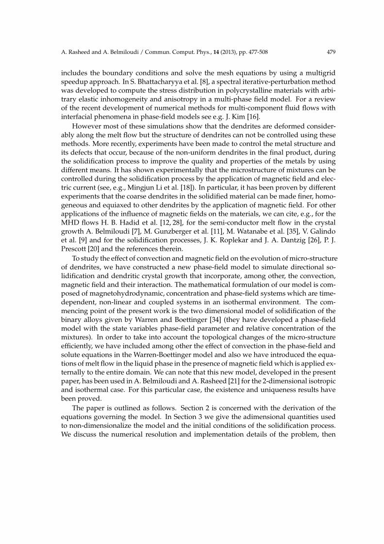
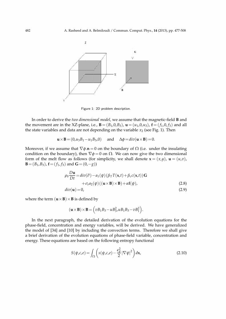
Figure 1: 2D problem description.
In order to derive the two dimensional model, we assume that the magnetic-field B andthe movement are in the XZ-plane, i.e., B=(B1,0,B3), u=(u1,0,u3), f=( f1,0, f3) and allthe state variables and data are not depending on the variable x2 (see Fig. 1). Then
u×B=(0,u3B1−u1B3,0) and ∆φ=div(u×B)=0.
Moreover, if we assume that ∇φ.n= 0 on the boundary of Ω (i.e. under the insulatingcondition on the boundary), then ∇φ= 0 on Ω. We can now give the two dimensionalform of the melt flow as follows (for simplicity, we shall denote x = (x,y), u = (u,v),B=(B1,B3), f=( f1, f3) and G=(0,−g))
ρ0Du
Dt=div(~σ)−a1(ψ)(βTT(x,t)+βcc(x,t))G
+σea2(ψ)((u×B)×B)+αf(ψ), (2.8)
div(u)=0, (2.9)
where the term (u×B)×B is defined by
(u×B)×B=(
vB1B3−uB23,uB1B3−vB2
1
)
.
In the next paragraph, the detailed derivation of the evolution equations for thephase-field, concentration and energy variables, will be derived. We have generalizedthe model of [34] and [10] by including the convection terms. Therefore we shall givea brief derivation of the evolution equations of phase-field variable, concentration andenergy. These equations are based on the following entropy functional
S(ψ,c,e)=∫
Ω
(
s(ψ,c,e)− ǫ2θ
2|∇ψ|2
)
dx, (2.10)
A. Rasheed and A. Belmiloudi / Commun. Comput. Phys., 14 (2013), pp. 477-508 483
where s(ψ,c,e) is an entropy density, e(x,t) is the internal energy, ψ(x,t) is the phase-fieldvariable and c(x,t) is the mole fraction of solute B in the solvent A. The second term inthe integrand is a gradient entropy term analogous to the gradient energy term in thefree energy, where the parameter ǫθ is the interfacial energy parameter which representsthe gradient corrections to the entropy density.
The phase field variable ψ(x,t) is not a conserved quantity therefore the most appro-priate form of the evolution equation for the phase field is defined by
Dψ
Dt=Mψ
δS(ψ,c,e)
δψ, (2.11)
where D/Dt=∂/∂t+(u·∇), Mψ>0 is the interfacial mobility parameter and the operatorδ denotes the variational derivative. The phase field variable ψ(x,t) varies smoothly inthe interval (0,1) and its value in the solid phase is 0 and in the liquid phase is 1.
The governing equations of the concentration c(x,t) and energy e(x,t) are derived byusing conservation laws of the concentration and the energy as
Dc
Dt=−div(Jc), (2.12)
De
Dt=−div(Je), (2.13)
where Jc and Je are the conserved flux of concentration and energy, respectively, whichcan be expressed by the irreversible linear laws as
Jc=Mc∇δS(ψ,c,e)
δc, (2.14)
Je =Me∇δS(ψ,c,e)
δe, (2.15)
where the parameters Mc and Me are assumed to be positive and are related to the A-B inter-diffusion coefficient and the heat conductivity, respectively, and S(ψ,c,e) is theentropy functional which is defined by Eq. (2.10).
Now we need to take the variational derivative of the functional S(ψ,c,e) in the senseof distribution. Let X be a topological space and U be an open set in X. Then the varia-tional derivative of Eq. (2.10) at ψ∈U in the direction of ξ∈D(U) is
⟨
δS(ψ,c,e)
δψ,ξ
⟩
D′(U),D(U)
=
⟨
∂s(ψ,c,e)
∂ψ,ξ
⟩
D′(U),D(U)
−⟨
∂
∂ψ
(
ǫ2θ
2|∇ψ|2
)
,ξ
⟩
D′(U),D(U)
, (2.16)
where D′(U) is the space of distributions corresponding to the space D(U) of test func-tions on U with compact support. Consider now the term
I=⟨
∂
∂ψ
(
ǫ2θ
2|∇ψ|2
)
,ξ
⟩
D′(U),D(U)
=∫
Ω
∂
∂ψ
(
ǫ2θ
2|∇ψ|2
)
ξdx
484 A. Rasheed and A. Belmiloudi / Commun. Comput. Phys., 14 (2013), pp. 477-508
and carrying out the differentiation in the integrand on the right hand side of the aboveequation with respect to ψ, we have
I=∫
Ω
(
ǫθ |∇ψ|2 ∂ǫθ
∂ψ·ξ+ǫ2
θ∇ψ·∇ξ
)
dx.
Since ǫθ is a function of θ, therefore by applying the chain rule and using divergencetheorem, we arrive at
I=∫
Ω
(
ǫθ |∇ψ|2 ∂ǫθ
∂θ
∂θ
∂ψ·ξ−div
(
ǫ2θ∇ψ
)
ξ
)
dx. (2.17)
Therefore the variational derivative of S can be given as
δS
δψ=
∂s
∂ψ+div
(
ǫ2θ∇ψ
)
−A
(
ǫθ ,ǫ′θ ,∂θ
∂ψ,∇ψ
)
, (2.18)
where ǫ′θ = ∂ǫθ/∂θ and A(
ǫθ ,ǫ′θ , ∂θ∂ψ ,∇ψ
)
= ǫθǫ′θ∂θ∂ψ |∇ψ|2. The variational derivative of S
with respect to c and e respectively, can easily be given (using (2.10)) as
δS
δc=
∂s
∂c, (2.19)
δS
δe=
∂s
∂e. (2.20)
In the above equations, the derivatives of the entropy density s(ψ,c,e) with respect to ψ, cand e are left to be determined and will be calculated using free energy density f (ψ,c,T).As we know from the basic thermodynamics that the free energy density can be definedby
f (ψ,c,T)= e(ψ,c,T)−Ts(ψ,c,e), (2.21a)
1
T=
∂s
∂e(ψ,c,e), (2.21b)
where e(ψ,c,T) and s(ψ,c,e) are the internal energy density and entropy density of thebinary alloy and T(x,t) is the temperature at any point in the time-space domain. Takingthe differential of the above equation we have
d f (ψ,c,T)=de(ψ,c,T)−Tds(ψ,c,e)−s(ψ,c,e)dT,
or
d f (ψ,c,T)=de(ψ,c,T)−T
(
∂s
∂ede+
∂s
∂ψdψ+
∂s
∂cdc
)
−s(ψ,c,e)dT,
and using the definition of the temperature (1/T = ∂s/∂e), the above equation takes theform
d f (ψ,c,T)=−T∂s
∂ψdψ−T
∂s
∂cdc−sdT. (2.22)
A. Rasheed and A. Belmiloudi / Commun. Comput. Phys., 14 (2013), pp. 477-508 485
Also as we know that
d f (ψ,c,T)=∂ f
∂ψdψ+
∂ f
∂cdc+
∂ f
∂TdT. (2.23)
Comparing Eqs. (2.22) and (2.23), we have the following relations
∂s(ψ,c,e)
∂ψ=− 1
T
∂ f (ψ,c,T)
∂ψ, (2.24)
∂s(ψ,c,e)
∂c=− 1
T
∂ f (ψ,c,T)
∂c, (2.25)
∂ f (ψ,c,T)
∂T=−s(ψ,c,e). (2.26)
An explicit relation of the free energy density f (ψ,c,T) of a binary alloy is given in [34] as
f (ψ,c,T)=(1−c)µA(ψ,c,T)+cµB(ψ,c,T), (2.27)
where µA(ψ,c,T) and µB(ψ,c,T) are the corresponding chemical potentials of the twoconstituent species A and B, and are defined as
µA(ψ,c,T)= fA(ψ,T)+λ(ψ)c2+RT
Vmln(1−c), (2.28)
µB(ψ,c,T)= fB(ψ,T)+λ(ψ)(1−c)2+RT
Vmln(c), (2.29)
where fA(ψ,T) and fB(ψ,T) are the free energy densities for substances A and B respec-tively, R is the universal gas constant, Vm is the molar volume and λ(ψ) is the regularsolution interaction parameter associated with the enthalpy of mixing and is assumed tobe
λ(ψ)=λS+p(ψ)(λL−λS),
where the parameters λS and λL are the enthalpies of mixing of the solid and liquidrespectively. Here it is assumed that the solution is ideal (similar as in [34]), therefore theparameters λS and λL are assumed to be zero and hence λ(ψ)=0.
Now using the basic thermodynamic, the relationship for the free energy density ofthe pure substance can be given as
f I(ψ,T)= eI(ψ,T)−TsI(ψ,T), I=A or B, (2.30)
where eI(ψ,T) is the internal energy density and sI(ψ,T) is the entropy density of the puresubstance I, with I = A or B. The internal energy density for each substance is assumedto have the form in [34] as
eI (ψ,T)= eI,S(T)+p(ψ)(eI,L(T)−eI,S(T)), I=A or B, (2.31)
486 A. Rasheed and A. Belmiloudi / Commun. Comput. Phys., 14 (2013), pp. 477-508
where eI,S(T) and eI,L(T) are the solid and liquid internal energies of the pure substancesI and are further defined as
eI,S(T)= eI,S(TIm)+CI
S(T−T Im), (2.32)
eI,L(T)= eI,L(TIm)+CI
L(T−T Im), (2.33)
where T Im is the melting temperature, CI
S and CIL are the heat capacities of solid and liq-
uid and eI,S(TIm) and eI,L(T
Im) are the internal energies of solid and liquid at the melting
temperature respectively of the substance I, where I= A or B. The factor p(ψ) should beselected here in the way that it is 0 in the solid phase to recover the internal energy den-sity of solid and 1 in the liquid phase to obtain the internal energy density of the liquidfor the pure substance I, that is, it should satisfy the following conditions
p(0)= p(1)=0, p′(ψ)>0 ∀ ψ ∈ ]0,1[. (2.34)
We shall elucidate further the choice of p(ψ) below. The latent heat of each pure substanceis defined as
LI = eI,L(TIm)−eI,S(T
Im), I=A or B, (2.35)
and by supposing that heat capacities are identical (i.e. CIS =CI
L=CI) for solid and liquidphase of each substance, we can write the final form of the internal energy densities ofeach substance using Eqs. (2.32), (2.33) and (2.35) as
eI (ψ,T)= eI,S(TIm)+CI(T−T I
m)+p(ψ)LI , I=A or B. (2.36)
Now using Eq. (2.26), Eq. (2.30) can be written as
f I(ψ,T)= eI(ψ,T)+T∂ f I
∂T(ψ,T), I=A or B,
which can further be written as
∂( f I /T)
∂T+
eI(ψ,T)
T2=0.
By integrating above equation with respect to T from T to T Im and using (2.36), we arrive
at
f I(ψ,T)=T
T Im
f I(ψ,T Im)+
(
eI,S(TIm)−CIT
Im+LI p(ψ)
)
(
1− T
T Im
)
−CIT ln
(
T
T Im
)
. (2.37)
Now the expression f I(ψ,T Im) is left only to be determined to achieve the final form of
the free energy density of each substance. The choice of f I(ψ,T Im) is dependent on the
phase field variable ψ as we should have the free energy density of the substance I in thesolid phase at ψ=0 and in the liquid phase at ψ=1. Also the free energy density shouldbe symmetric at the melting temperature with respect to ψ= 1/2. Thus the free energy
A. Rasheed and A. Belmiloudi / Commun. Comput. Phys., 14 (2013), pp. 477-508 487
density f I(ψ,T Im) that follows these conditions can be chosen as a function g(ψ) of class
C2([0,1],R) which satisfies the following conditions
g(0)= g(1)=0,g′(ψ)=0 iff ψ∈0,1/2,1 ,g′′(0), g′′(1)>0,g(ψ)= g(1−ψ).
(2.38)
The function g can be chosen as
g(ψ)=ψ2(1−ψ)2, (2.39)
which is a double well polynomial function of the minimum degree that satisfies theproperties defined in (2.38). More details about the choice and properties of the functiong(ψ) can be found in [34]. Therefore the form of f I(ψ,T I
m) is assumed to be
f I(ψ,T Im)=T I
mWI ψ2(1−ψ)2, (2.40)
where WI is the constant which controls the height of the well and is defined as
WI =3σI√2T I
mδI
, I=A or B, (2.41)
where σI is the solid-liquid interface energy, T Im is the melting temperature and δI is the
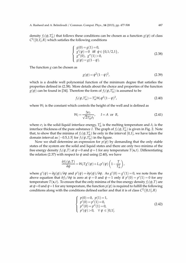
interface thickness of the pure substance I. The graph of f I(ψ,T Im) is given in Fig. 2. Note
that, to show that the minima of f I(ψ,T Im) lie only in the interval [0,1], we have taken the
domain interval as [−0.5,1.5] for f I(ψ,T Im) in the figure.
Now we shall determine an expression for p(ψ) by demanding that the only stablestates of the system are the solid and liquid states and there are only two minima of thefree energy density f I(ψ,T) at ψ=0 and ψ=1 for any temperature T(x,t). Differentiatingthe relation (2.37) with respect to ψ and using (2.40), we have
∂ f I(ψ,T)
∂ψ=WI Tg′(ψ)+LI p′(ψ)
(
1− T
T Im
)
,
where g′(ψ)= ∂g(ψ)/∂ψ and p′(ψ)= ∂p(ψ)/∂ψ. As g′(0)= g′(1)= 0, we note from theabove equation that ∂ f I /∂ψ is zero at ψ = 0 and ψ = 1 only if p′(0) = p′(1) = 0 for anytemperature T(x,t). To ensure that the only minima of the free energy density f I(ψ,T) areat ψ=0 and ψ=1 for any temperature, the function p(ψ) is required to fulfill the followingconditions along with the conditions defined earlier and that it is of class C2([0,1],R)
p(0)=0, p(1)=1,p′(0)= p′(1)=0,p′′(0)= p′′(1)=0,p′(ψ)>0, ∀ ψ ∈ ]0,1[.
(2.42)
488 A. Rasheed and A. Belmiloudi / Commun. Comput. Phys., 14 (2013), pp. 477-508
−0.5 0 0.5 1 1.50
0.02
0.04
0.06
0.08
Figure 2: The graph of f I(ψ,T Im).
−0.5 0 0.5 1 1.5−3
−2
−1
0
1
2
3
4
Figure 3: The graph of function p(ψ).
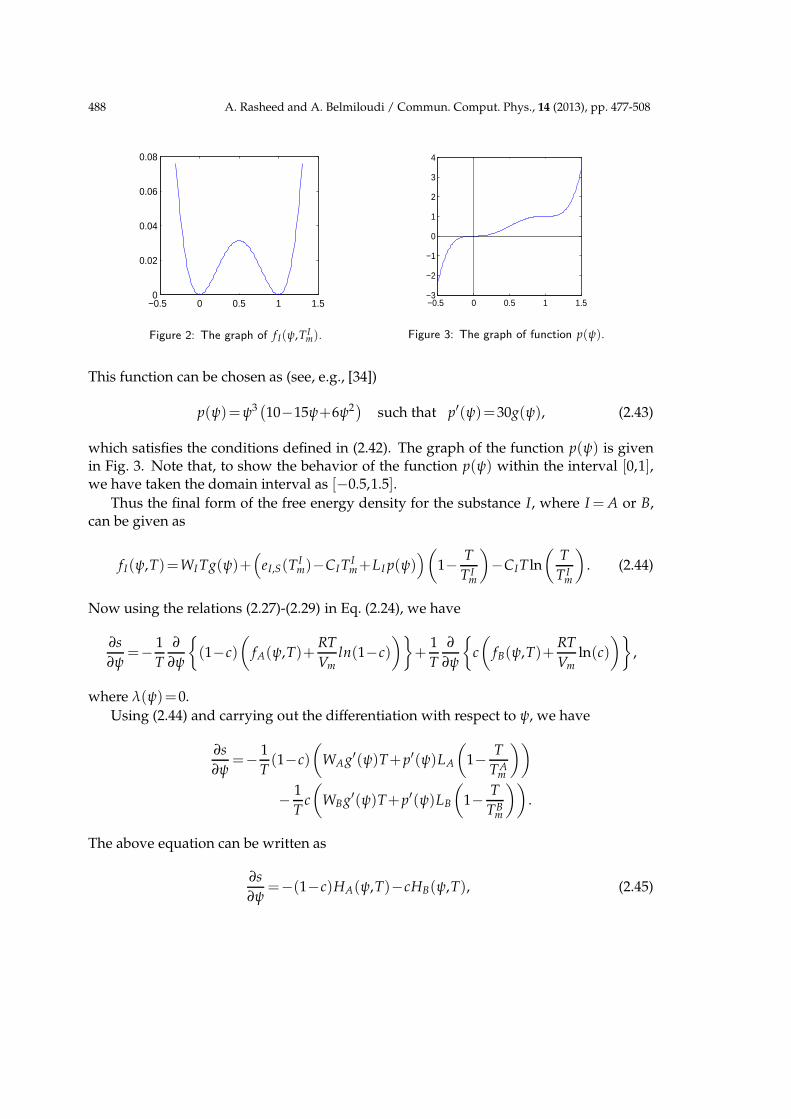
This function can be chosen as (see, e.g., [34])
p(ψ)=ψ3(
10−15ψ+6ψ2)
such that p′(ψ)=30g(ψ), (2.43)
which satisfies the conditions defined in (2.42). The graph of the function p(ψ) is givenin Fig. 3. Note that, to show the behavior of the function p(ψ) within the interval [0,1],we have taken the domain interval as [−0.5,1.5].
Thus the final form of the free energy density for the substance I, where I = A or B,can be given as
f I(ψ,T)=WI Tg(ψ)+(
eI,S(TIm)−CI T
Im+LI p(ψ)
)
(
1− T
T Im
)
−CIT ln
(
T
T Im
)
. (2.44)
Now using the relations (2.27)-(2.29) in Eq. (2.24), we have
∂s
∂ψ=− 1
T
∂
∂ψ
(1−c)
(
fA(ψ,T)+RT
Vmln(1−c)
)
+1
T
∂
∂ψ
c
(
fB(ψ,T)+RT
Vmln(c)
)
,
where λ(ψ)=0.
Using (2.44) and carrying out the differentiation with respect to ψ, we have
∂s
∂ψ=− 1
T(1−c)
(
WAg′(ψ)T+p′(ψ)LA
(
1− T
TAm
))
− 1
Tc
(
WBg′(ψ)T+p′(ψ)LB
(
1− T
TBm
))
.
The above equation can be written as
∂s
∂ψ=−(1−c)HA(ψ,T)−cHB(ψ,T), (2.45)
A. Rasheed and A. Belmiloudi / Commun. Comput. Phys., 14 (2013), pp. 477-508 489
where (since p′(ψ)=30g(ψ))
HA(ψ,T)=WAg′(ψ)+30g(ψ)LA
(
1
T− 1
TAm
)
, (2.46)
HB(ψ,T)=WBg′(ψ)+30g(ψ)LB
(
1
T− 1
TBm
)
, (2.47)
where g′(ψ)=∂g(ψ)/∂ψ.Substituting Eq. (2.45) into Eq. (2.18) and then the resulting equation in Eq. (2.11), we
obtain the following equation
Dψ
Dt=Mψ
(
div(
ǫ2θ∇ψ
)
−(1−c)HA(ψ,T)−cHB(ψ,T)−A(
ǫθ ,ǫ′θ ,∂θ
∂ψ,∇ψ
))
, (2.48)
which is the general equation of phase-field, where the operators A and div(
ǫ2θ∇ψ
)
areleft to be calculated. We can compute these operators by introducing the operator ǫθ .
In two dimensional geometry, the parameter ǫθ is assumed to be anisotropic and is de-fined as [34]
ǫθ =ǫ0η=ǫ0(1+γ0coskθ), (2.49)
where anisotropic means that ǫθ is dependent on the direction of the solid-liquid inter-face, γ0 is the anisotropic amplitude, k the mode number, ǫ0 is a constant and
θ=arctan
(
ψy
ψx
)
, (2.50)
is the angle between the local interface normal and a designated base vector of the crystallattice, subscripts x and y are used to denote the partial derivatives with respect to spatialcoordinates, that is, ψx =∂ψ/∂x and ψy=∂ψ/∂y.
Remark 2.2. The anisotropy plays an important role in modeling the dendritic solidifi-cation process. In fact, for example, for the metal alloys, the form of dendrites is usuallysymmetric and has four major dendrite arms and minor arms around them. In the solid-ification model, the mode number k, in the anisotropy function ǫθ , usually represents thedendrite arms. If we want to obtain a dendrite with four arms, we fix the value of k equalto 4. Its value depends on the form of dendrites obtained in a particular alloy.
By calculating the operators A and div(
ǫ2θ∇ψ
)
(according to the expression of ǫθ andθ, we can deduce, from (2.48), the following two dimensional model
Dψ
Dt=Mψ
(
ǫ20η2
∆ψ−(1−c)HA(ψ,T)−cHB(ψ,T))
−Mψǫ2
0
(
ηη′′+(η′)2)
2
2ψxy sin2θ−∆ψ−(
ψyy−ψxx
)
cos2θ
+Mψǫ20ηη′sin2θ
(
ψyy−ψxx
)
+2ψxy cos2θ
, (2.51)
490 A. Rasheed and A. Belmiloudi / Commun. Comput. Phys., 14 (2013), pp. 477-508
which is the final form of the evolution equation for the phase-field ψ(x,t), where weassume Mψ to be a positive constant.
If we assume that the interface thickness δA = δB = δ in the parameters defined in therelation (2.41), then Eq. (2.51) can be simplified and takes the form
Dψ
Dt=Mψǫ2
0
(
η2∆ψ− λ1(c)
δ2g′(ψ)− 1
δλ2(c)p′(ψ)
)
−Mψǫ2
0
(
ηη′′+(η′)2)
2
2ψxysin2θ−∆ψ−(
ψyy−ψxx
)
cos2θ
+Mψǫ20ηη′
sin2θ(
ψyy−ψxx
)
+2ψxycos2θ
, (2.52)
where
ǫ20 =
3√
2(σA+σB)δ
Tm, Tm =
TAm +TB
m
2, (2.53a)
λ1(c)=(1−c)λ1A+cλ1B, λ2(c)=(1−c)λ2A+cλ2B, (2.53b)
with
λ1A =σA
(σA+σB)
Tm
TAm
, λ1B =σB
(σA+σB)
Tm
TBm
,
λ2A =LATm
3√
2(σA+σB)
(
1
T− 1
TAm
)
, λ2B =LBTm
3√
2(σA+σB)
(
1
T− 1
TAm
)
.
Now we present the derivation of the concentration and energy equations. It is ob-served by Warren and Boettinger [34] that the terms ∇T in the concentration equation(2.12) and ∇c in the energy equation (2.13) are the small corrections. Therefore, in thederivation of the concentration equation, we shall assume that the temperature T(x,t)is constant and in the derivation of energy equation, the concentration c(x,t) will be as-sumed fixed.
By employing Eqs. (2.27), (2.25) and (2.19), Eq. (2.14) takes the form
Jc=Mc∇(
−µB(ψ,c,T)−µA(ψ,c,T)
T(x,t)
)
.
Since temperature T(x,t) is assumed to be constant, therefore the above equation can bewritten as
Jc=−Mc
T∇(µB(ψ,c,T)−µA(ψ,c,T)) .
With the help of Eqs. (2.28) and (2.29), the above equation takes the form
Jc=−Mc
T
(
∇ fB(ψ,T)+RT
Vm
1
c∇c
)
+Mc
T
(
∇ fA(ψ,T)+RT
Vm
1
1−c(−∇c)
)
.
A. Rasheed and A. Belmiloudi / Commun. Comput. Phys., 14 (2013), pp. 477-508 491
Making use of the relation (2.44), we obtain
Jc=Mc
(
−WBg′(ψ)−p′(ψ)LB
(
1
T− 1
TBm
))
∇ψ
+Mc
(
WAg′(ψ)+p′(ψ)LA
(
1
T− 1
TAm
))
∇ψ
+Mc
(
− R
Vm
1
c∇c− R
Vm
1
1−c(∇c)
)
.
Using the relations (2.46) and (2.47) in the above equation, we have
Jc=Mc(HA(ψ,T)−HB(ψ,T))∇ψ− McR
Vmc(1−c)∇c. (2.54)
Also the comparison of Eq. (2.54) with the Fick’s first law in a single-phase system (i.e.,with ∇ψ=0) establishes the relation given below [34]
Mc=D(ψ)Vmc(1−c)
R, (2.55)
where D(ψ)=DS+p(ψ)(DL−DS) is the A-B inter-diffusion coefficient.Substituting (2.55) into Eq. (2.54), we obtain
Jc=D(ψ)Vmc(1−c)
R(HA(ψ,T)−HB(ψ,T))∇ψ−D(ψ)∇c. (2.56)
Finally substituting Eq. (2.56) into Eq. (2.12), we have
Dc
Dt=div
(
D(ψ)
(
∇c+c(1−c)Vm
R(HB(ψ,T)−HA(ψ,T))∇ψ
))
. (2.57)
Eq. (2.57) represents the final form of the evolution equation for the mole fraction (con-centration) of the solute.
If we assume that the interface thickness δA = δB = δ in the parameters defined in theexpression (2.41), then the above equation reduces to the following equation
Dc
Dt=div(D(ψ)∇c)+div
(
α0D(ψ)c(1−c)
1
δλ′
1(c)g′(ψ)+λ′2(c)p′(ψ)
∇ψ
)
, (2.58)
where
α0=3√
2Vm
RTm(σA+σB), (2.59)
with λ′1(c)=∂λ(c)/∂c, λ′
2(c)=∂λ(c)/∂c, where λ1(c) and λ2(c) are defined in (2.53).For the derivation of the evolution equation for the energy, first, the internal energy
density of a binary alloy can be expressed using a rule of mixture as (e.g., [10])
e(ψ,c,T)=(1−c)eA(ψ,T)+c eB(ψ,T). (2.60)
492 A. Rasheed and A. Belmiloudi / Commun. Comput. Phys., 14 (2013), pp. 477-508
Using the definition of the temperature ∂s/∂e=1/T into Eqs. (2.20) and (2.15) we get
Je =Me
(
− 1
T2∇T(x,t)
)
. (2.61)
Now substituting (2.60) and (2.61) in Eq. (2.13), we have
D
Dt((1−c)eA(ψ,T)+c eB(ψ,T))=−∇·
(
Me
(
− 1
T2∇T(x,t)
))
.
Since concentration c(x,t) is considered constant in the derivation of the energy equation,therefore the above equation takes the form
(1−c)DeA(ψ,T)
Dt+c
DeB(ψ,T)
Dt=−∇·
(
Me
(
− 1
T2∇T(x,t)
))
.
By using (2.36) and setting Me = KT2, where K is the thermal conductivity, the aboveequation becomes
(1−c)
(
CADT
Dt+LA
Dp(ψ)
Dt
)
+c
(
CBDT
Dt+LB
Dp(ψ)
Dt
)
=∇·(K∇T).
Applying chain rule and re-arranging the above equation, we have
((1−c)CA+cCB)DT
Dt+((1−c)LA+cLB)p′(ψ)
Dψ
Dt=∇·(K∇T).
Further the above equation can be written as
CDT(x,t)
Dt+30L g(ψ)
Dψ(x,t)
Dt=∇·(K∇T(x,t)), (2.62)
where
C=(1−c)CA+cCB,
L=(1−c)LA+cLB,
K=(1−c)KA+cKB,
with KA and KB, the thermal conductivities of substances A and B respectively. Eq. (2.62)represents the final form of the evolution equation for the temperature field T(x,t).
We can now summarize the governing equations of the model.
A. Rasheed and A. Belmiloudi / Commun. Comput. Phys., 14 (2013), pp. 477-508 493
2.2 The governing equations of the model
2.2.1 General model
In this section, we shall summarize the entire set of governing equations that model thesolidification process of a binary alloy in a non-isothermal environment in the presence ofmotion in the liquid phase with the magnetic field effect. The equations that model thisphenomenon are the phase-field equation (2.48), concentration equation (2.57), energyequation (2.62) and the melt flow system (2.4), (2.5) and (2.6) which are given below
ρ0Du
Dt=div(~σ)+a1(ψ)(−βTT(x,t)−βcc(x,t))G
+a2(ψ)σe(−∇φ+u×B)×B+αf(ψ) on Q, (2.63a)
div(u)=0 on Q, (2.63b)
Dψ
Dt=Mψ
(
div(
ǫ2θ∇ψ
)
−(1−c)HA(ψ,T)−cHB(ψ,T)−A(
ǫθ ,ǫ′θ ,∂θ
∂ψ,∇ψ
))
on Q, (2.63c)
Dc
Dt=div
(
D(ψ)
(
∇c+c(1−c)Vm
R(HB(ψ,T)−HA(ψ,T))∇ψ
))
on Q, (2.63d)
CDT
Dt+30L g(ψ)
∂ψ
∂t=∇·(K∇T) on Q, (2.63e)
∆φ=div(u×B) on Q, (2.63f)
where ~σ=−pI+µ(
∇u+(∇u)tran)
, Q=Ω×(
0,Tf
)
, Tf is the solidification time and theexpressions for the nonlinear operators and for the parameters are defined earlier. In thecase of an isothermal process, the model (2.63) can be reduced to
ρ0Du
Dt=div(~σ)−a1(ψ)βcc(x,t)G+a2(ψ)σe(−∇φ+u×B)×B+αf(ψ) on Q, (2.64a)
div(u)=0 on Q, (2.64b)
Dψ
Dt=Mψ
(
div(
ǫ2θ∇ψ
)
−(1−c)HA(ψ)−cHB(ψ)−A(
ǫθ ,ǫ′θ ,∂θ
∂ψ,∇ψ
))
on Q, (2.64c)
Dc
Dt=div
(
D(ψ)
(
∇c+c(1−c)Vm
R
(
HB(ψ)−HA(ψ))
∇ψ
))
on Q, (2.64d)
∆φ=div(u×B) on Q, (2.64e)
where
f(ψ)=− a1(ψ)βTTG
α+f(ψ) and HI(ψ)=HI(ψ,T)
for I=A,B.
Next we shall reduce the previous systems to the two dimensional geometry.
494 A. Rasheed and A. Belmiloudi / Commun. Comput. Phys., 14 (2013), pp. 477-508
2.2.2 Two dimensional geometry
In a two dimensional case, we have worked in the XZ-plane and we have supposed that∇φ.n=0 on the boundary of the solidification domain Ω. According to (2.8), (2.49), (2.50)and (2.51), the two dimensional model is
ρ0Du
Dt=div(~σ)+a1(ψ)(−βTT(x,t)−βcc(x,t))G
+a2(ψ)σe(u×B)×B+αf(ψ) on Q, (2.65a)
div(u)=0 on Q, (2.65b)
Dψ
Dt=Mψ
(
ǫ20η2
∆ψ−(1−c)HA(ψ,T)−cHB(ψ,T))
−Mψǫ2
0
(
ηη′′+(η′)2)
2
2ψxy sin2θ−∆ψ−(
ψyy−ψxx
)
cos2θ
+Mψǫ20ηη′sin2θ
(
ψyy−ψxx
)
+2ψxycos2θ
on Q, (2.65c)
Dc
Dt=div
(
D(ψ)
(
∇c+c(1−c)Vm
R(HB(ψ,T)−HA(ψ,T))∇ψ
))
on Q, (2.65d)
CDT
Dt+30L g(ψ)
∂ψ
∂t=∇·(K∇T) on Q. (2.65e)
In the case of an isothermal process, the model (2.65) is reduced to
ρ0Du
Dt=div(~σ)−a1(ψ)βcc(x,t)G+a2(ψ)σe(u×B)×B+αf(ψ) on Q, (2.66a)
div(u)=0 on Q, (2.66b)
Dψ
Dt=Mψ
(
ǫ20η2
∆ψ−(1−c)HA(ψ)−cHB(ψ))
−Mψǫ2
0
(
ηη′′+(η′)2)
2
2ψxysin2θ−∆ψ−(
ψyy−ψxx
)
cos2θ
+Mψǫ20ηη′sin2θ
(
ψyy−ψxx
)
+2ψxycos2θ
on Q, (2.66c)
Dc
Dt=div
(
D(ψ)
(
∇c+c(1−c)Vm
R
(
HB(ψ)−HA(ψ))
∇ψ
))
on Q. (2.66d)
Nota Bene: In the sequel, we omit the ” ˜ ” in the system (2.66).
We assume that there exists a unique solution (u,ψ,c) of the problem (2.66), undersome hypotheses for data and some regularity of the nonlinear operators. In particular,for the isotropic case of the model (2.66), we have proved the existence and the unique-ness results in [21]. In the next section, we shall present the numerical simulations ofthe dendrite growth during the solidification of a Ni-Cu (Nickel-Copper) binary mixture.To perform these simulations, we consider the two dimensional and isothermal model(2.66). We further suppose that the interface thicknesses for both substances are equali.e., δA =δB=δ.
A. Rasheed and A. Belmiloudi / Commun. Comput. Phys., 14 (2013), pp. 477-508 495
3 Numerical study
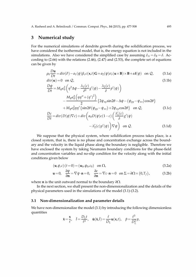
For the numerical simulations of dendrite growth during the solidification process, wehave considered the isothermal model, that is, the energy equation is not included in thesimulations. Also we have considered the simplified case by assuming δA = δB = δ. Ac-cording to (2.66) with the relations (2.46), (2.47) and (2.53), the complete set of equationscan be given by
ρ0Du
Dt=div(~σ)−a1(ψ)βcc(x,t)G+a2(ψ)σe(u×B)×B+αf(ψ) on Q, (3.1a)
div(u)=0 on Q, (3.1b)
Dψ
Dt=Mψǫ2
0
(
η2∆ψ− λ1(c)
δ2g′(ψ)− λ2(c)
δp′(ψ)
)
−Mψǫ2
0
(
ηη′′+(η′)2)
2
2ψxysin2θ−∆ψ−(
ψyy−ψxx
)
cos2θ
+Mψǫ20ηη′sin2θ
(
ψyy−ψxx
)
+2ψxycos2θ
on Q, (3.1c)
Dc
Dt=div(D(ψ)∇c)+div
(
α0D(ψ)c(1−c)
(
λ′1(c)
δg′(ψ)
−λ′2(c)p′(ψ)
)
∇ψ
)
on Q. (3.1d)
We suppose that the physical system, where solidification process takes place, is aclosed system, that is, there is no phase and concentration exchange across the bound-ary and the velocity in the liquid phase along the boundary is negligible. Therefore wehave enclosed the system by taking Neumann boundary conditions for the phase-fieldand concentration variables and no-slip condition for the velocity along with the initialconditions given below
(u,ψ,c)(t=0)=(u0,ψ0,c0) on Ω, (3.2a)
u=0,∂ψ
∂n=∇ψ·n=0,
∂c
∂n=∇c·n=0 on Σ=∂Ω×
(
0,Tf
)
, (3.2b)
where n is the unit outward normal to the boundary ∂Ω.In the next section, we shall present the non-dimensionalization and the details of the
physical parameters used in the simulations of the model (3.1)-(3.2).
3.1 Non-dimensionalization and parameter details
We have non-dimensionalize the model (3.1) by introducing the following dimensionlessquantities
x=x
ℓ, t=
DLt
ℓ2, u(x, t)=
ℓ
DLu(x,t), p=
ℓ3
D2L
p,
496 A. Rasheed and A. Belmiloudi / Commun. Comput. Phys., 14 (2013), pp. 477-508
B=B
B0, ψ(x, t)=ψ(x,t), c(x, t)= c(x,t), (3.3)
where x and t are the dimensionless spatial and time coordinates, u, ψ, and c are thenondimensional velocity-field, phase-field and concentration respectively, ℓ is the char-acteristic length of the domain Ω, ℓ2/DL is the liquid diffusion time, DL is the solutaldiffusivity in liquid and B0 is the characteristic magnetic-field. Note that the phase-fieldis a mathematical quantity and c is the relative concentration which are already dimen-sionless quantities. Using these adimensional relations, we get finally the dimensionlessform of the model as
Du
Dt= ˜div(−pI+Pr(∇u+(∇u)tran)+PrRaca1(ψ)ceG
+Pr(Ha)2a2(ψ)(u×B)×B+Krf(ψ) on Q= Ω×(
0,t f
)
, (3.4a)
˜div(u)=0 on Q, (3.4b)
Dψ
Dt=ǫ2
(
η2∆ψ− λ1(c)
δ2g′(ψ)− λ2(c)
δp′(ψ)
)
−ǫ2
(
ηη′′+(η′)2)
2
2ψxy sin2θ−∆ψ−(
ψyy−ψxx
)
cos2θ
+ǫ2ηη′sin2θ(
ψyy−ψxx
)
+2ψxycos2θ
on Q, (3.4c)
Dc
Dt= ˜div
(
D(ψ)∇c)
+ ˜div
(
α0D(ψ)c(1− c)
(
λ′1(c)
δg′(ψ)
−λ′2(c)p′(ψ)
)
∇ψ
)
on Q, (3.4d)
with the initial and boundary conditions
(u,ψ, c)(t=0)=(u0,ψ0, c0) on Ω, (3.5a)
u=0,∂ψ
∂n=0,
∂c
∂n=0 on Σ=∂Ω×
(
0,t f
)
, (3.5b)
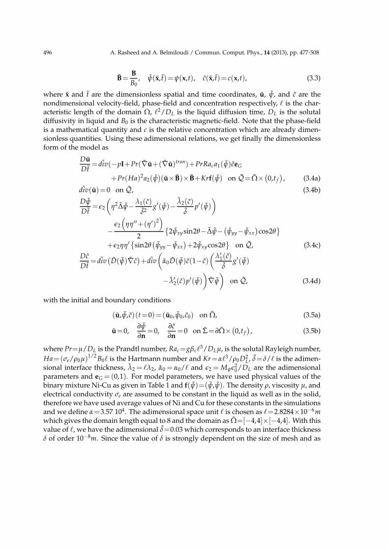
where Pr=µ/DL is the Prandtl number, Rac=gβcℓ3/DLµ, is the solutal Rayleigh number,
Ha=(σe/ρ0µ)1/2 B0ℓ is the Hartmann number and Kr=αℓ3/ρ0D2L, δ=δ/ℓ is the adimen-
sional interface thickness, λ2 = ℓλ2, α0 = α0/ℓ and ǫ2 = Mψǫ20/DL are the adimensional
parameters and eG =(0,1). For model parameters, we have used physical values of thebinary mixture Ni-Cu as given in Table 1 and f(ψ)=(ψ,ψ). The density ρ, viscosity µ, andelectrical conductivity σe are assumed to be constant in the liquid as well as in the solid,therefore we have used average values of Ni and Cu for these constants in the simulationsand we define α=3.57 104. The adimensional space unit ℓ is chosen as ℓ=2.8284×10⁻⁶mwhich gives the domain length equal to 8 and the domain as Ω=[−4,4]×[−4,4]. With thisvalue of ℓ, we have the adimensional δ=0.03 which corresponds to an interface thicknessδ of order 10−8m. Since the value of δ is strongly dependent on the size of mesh and as
A. Rasheed and A. Belmiloudi / Commun. Comput. Phys., 14 (2013), pp. 477-508 497
Table 1: Physical values of constants.
Property Name Symbol Unit Nickel Copper
Melting temperature Tm K 1728 1358
Latent heat L J/m3 2350×106 1758×106
Diffusion coeff. liquid DL m2/s 10−9 10−9
Diffusion coeff. solid DS m2/s 10−13 10−13
Linear kinetic coeff. β m/K/s 3.3×10⁻³ 3.9×10⁻³
Interface thickness δ m 8.4852×10⁻⁸ 6.0120×10⁻⁸
Density ρ Kg/m3 7810 8020
viscosity µ Pa·s 4.110×10⁻⁶ 0.597×10⁻⁶
Surface energy σ J/m2 0.37 0.29
Electrical conductivity σe S/m 14.3×10⁶ 59.6×10⁶
Molar volume Vm m3 7.46×10⁻⁶ 7.46×10⁻⁶
Mode Number k N/A 4 4
Anisotropy Amplitude γ0 N/A 0.04 0.04
the mesh size should be sufficiently less than the interface thickness δ and we have useda coarse mesh for our simulations due to technical difficulties in computations, thereforewe fix the value of the adimensional interface thickness as δ= 0.05 for our simulationsto ensure the mesh size less than the interface thickness. The adimensional final time ist f =0.13, which corresponds to the real physical final time of Tf =1 ms. Note that big timesteps and smaller interface values can create convergence problems during the calcula-tion of numerical solution of the problem. We choose the values of the physical constants(see Table 1) for the phase-field and concentration equations in our model as given in [34]and the constants associated with the flow equations are chosen by keeping in view theproperties of substances A (Copper (Cu) in the present case) and B (Nickel (Ni) in thepresent case).
Nota Bene: the use of ”˜” for the variables x,y and t will now be omitted.
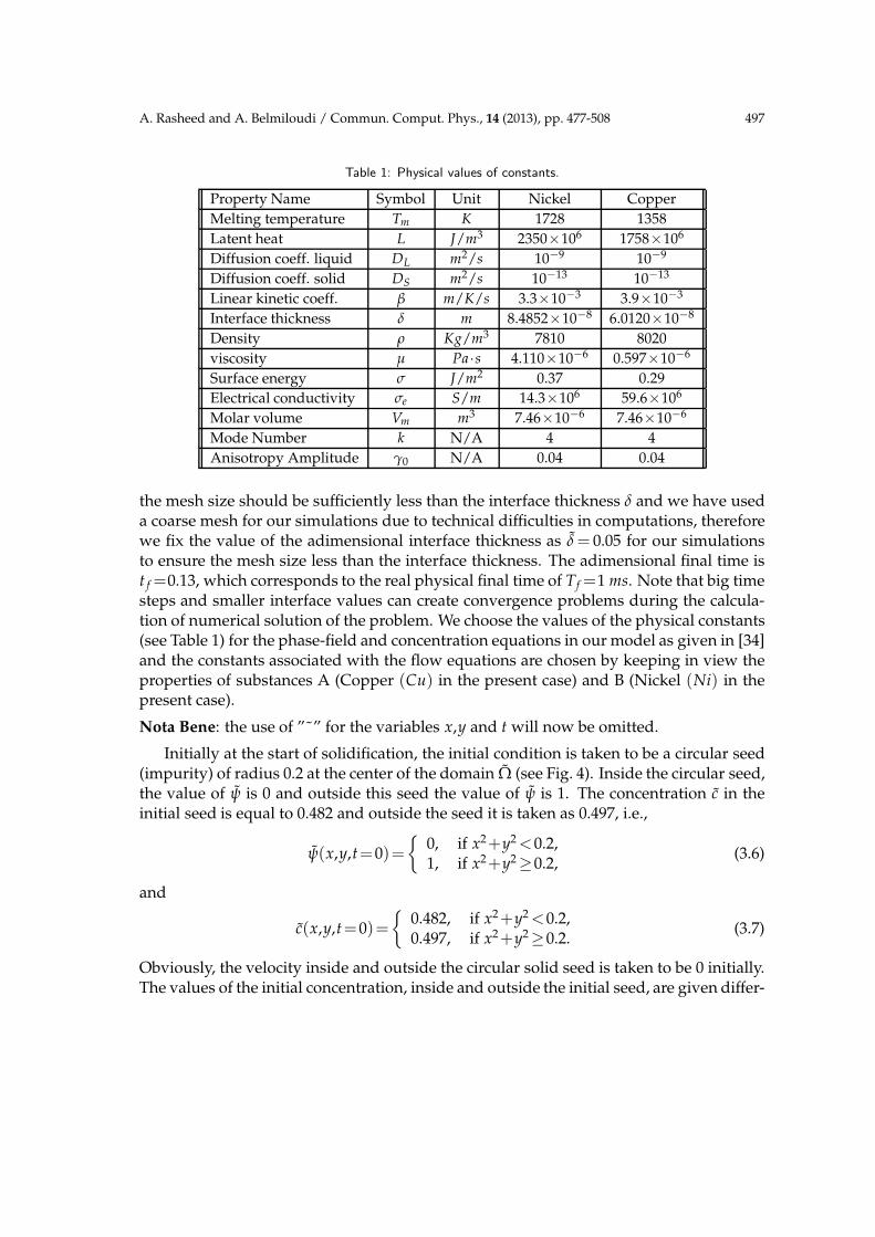
Initially at the start of solidification, the initial condition is taken to be a circular seed(impurity) of radius 0.2 at the center of the domain Ω (see Fig. 4). Inside the circular seed,the value of ψ is 0 and outside this seed the value of ψ is 1. The concentration c in theinitial seed is equal to 0.482 and outside the seed it is taken as 0.497, i.e.,
ψ(x,y,t=0)=
0, if x2+y2<0.2,1, if x2+y2≥0.2,
(3.6)
and
c(x,y,t=0)=
0.482, if x2+y2<0.2,0.497, if x2+y2≥0.2.
(3.7)
Obviously, the velocity inside and outside the circular solid seed is taken to be 0 initially.The values of the initial concentration, inside and outside the initial seed, are given differ-
498 A. Rasheed and A. Belmiloudi / Commun. Comput. Phys., 14 (2013), pp. 477-508
Figure 4: Geometry of the domain.
ent by different authors depending on the phase diagram of binary mixture Ni-Cu (see,e.g,. [10, 15, 34]).
3.2 Numerical scheme and implementation details
In this section we elaborate the numerical resolution of the problem (3.4). First, we dis-cretize the problem with respect to spatial coordinates using mixed finite elements, whichsatisfy the InfSup condition (Babuska-Brezi’s condition), for the velocity u and pressure pin the system (3.4a)-(3.4b) and the usual finite elements for phase-field ψ and concentra-tion c in the equations (3.4c) and (3.4d) respectively. More precisely we have used mixedfinite elements Pi−Pi−1 for the velocity u and pressure p and Pi for the phase-field ψand concentration c, respectively, where Pi is the polynomial of degree i. We obtain asystem of nonlinear ordinary differential equations. The derived non-linear systems arethen solved by using solver DASSL: for the time discretization, we have used back-warddifference Euler’s formula and the resulting non-linear systems are solved using New-ton method (for more details about the solver DASSL see e.g., [19]). To implement thedeveloped method, we have employed Comsol together with Matlab tools.
Remark 3.1. Before employing the developed numerical scheme to perform numericalsimulations of the model in the case of Ni-Cu, we have studied the convergence (bothwith respect to space and time variables) and stability of the scheme by considering sev-eral examples with known exact solutions (with parameters and data corresponding tothe mixture Ni-Cu). We have demonstrated numerically that the error estimates withrespect to space are of order i+1 for velocity u, phase-field ψ and concentration c andof order i for the pressure p, and the error estimates with respect to time are of order1 for (u, p,ψ, c). The stability of the scheme has also been studied by introducing a ran-dom function, which varies between 0 and 1, in the model. We found that the numericalscheme is convergent and stable.
A. Rasheed and A. Belmiloudi / Commun. Comput. Phys., 14 (2013), pp. 477-508 499
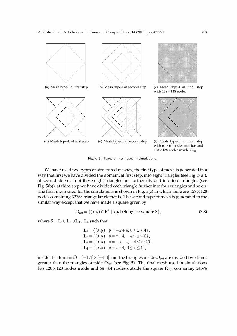
(a) Mesh type-I at first step (b) Mesh type-I at second step (c) Mesh type-I at final stepwith 128×128 nodes
(d) Mesh type-II at first step (e) Mesh type-II at second step (f) Mesh type-II at final stepwith 64×64 nodes outside and128×128 nodes inside Ωint
Figure 5: Types of mesh used in simulations.
We have used two types of structured meshes, the first type of mesh is generated in away that first we have divided the domain, at first step, into eight triangles (see Fig. 5(a)),at second step each of these eight triangles are further divided into four triangles (seeFig. 5(b)), at third step we have divided each triangle further into four triangles and so on.The final mesh used for the simulations is shown in Fig. 5(c) in which there are 128×128nodes containing 32768 triangular elements. The second type of mesh is generated in thesimilar way except that we have made a square given by
Ωint=
(x,y)∈R2 | x,y belongs to square S
, (3.8)
where S=L1∪L2∪L3∪L4 such that
L1=(x,y) | y=−x+4, 0≤ x≤4 ,
L2=(x,y) | y= x+4, −4≤ x≤0 ,
L3=(x,y) | y=−x−4, −4≤ x≤0 ,
L4=(x,y) | y= x−4, 0≤ x≤4 ,
inside the domain Ω=[−4,4]×[−4,4] and the triangles inside Ωint are divided two timesgreater than the triangles outside Ωint (see Fig. 5). The final mesh used in simulationshas 128×128 nodes inside and 64×64 nodes outside the square Ωint containing 24576
500 A. Rasheed and A. Belmiloudi / Commun. Comput. Phys., 14 (2013), pp. 477-508
triangular elements (see Fig. 5(f)). The second kind of mesh is used to save the time andto reduce memory requirement without having effect on the results.
We have used two types of finite elements to solve the problem (3.4). First is P2−P1
for the magnetohydrodynamic type system and P2 finite elements for the phase-fieldand concentration equations respectively. Second is the P3−P2 for the magnetohydrody-namic type system and P3 for the phase-field and concentration equations of the problem(3.4). It is important to mention that using first kind of finite elements and type-I mesh,it takes approximately 29 hours and using type-II mesh takes approximately 18 hours tocomplete one simulation. And using second type of finite elements with type-II mesh, ittakes about 8 days to execute one simulation using the hardware defined below.
To carry out all simulations we have used a Dell Laptop computer with 4GB of com-puter memory and 2GHz core2 dual processor with 64−bit Vista windows.
3.3 Numerical simulations
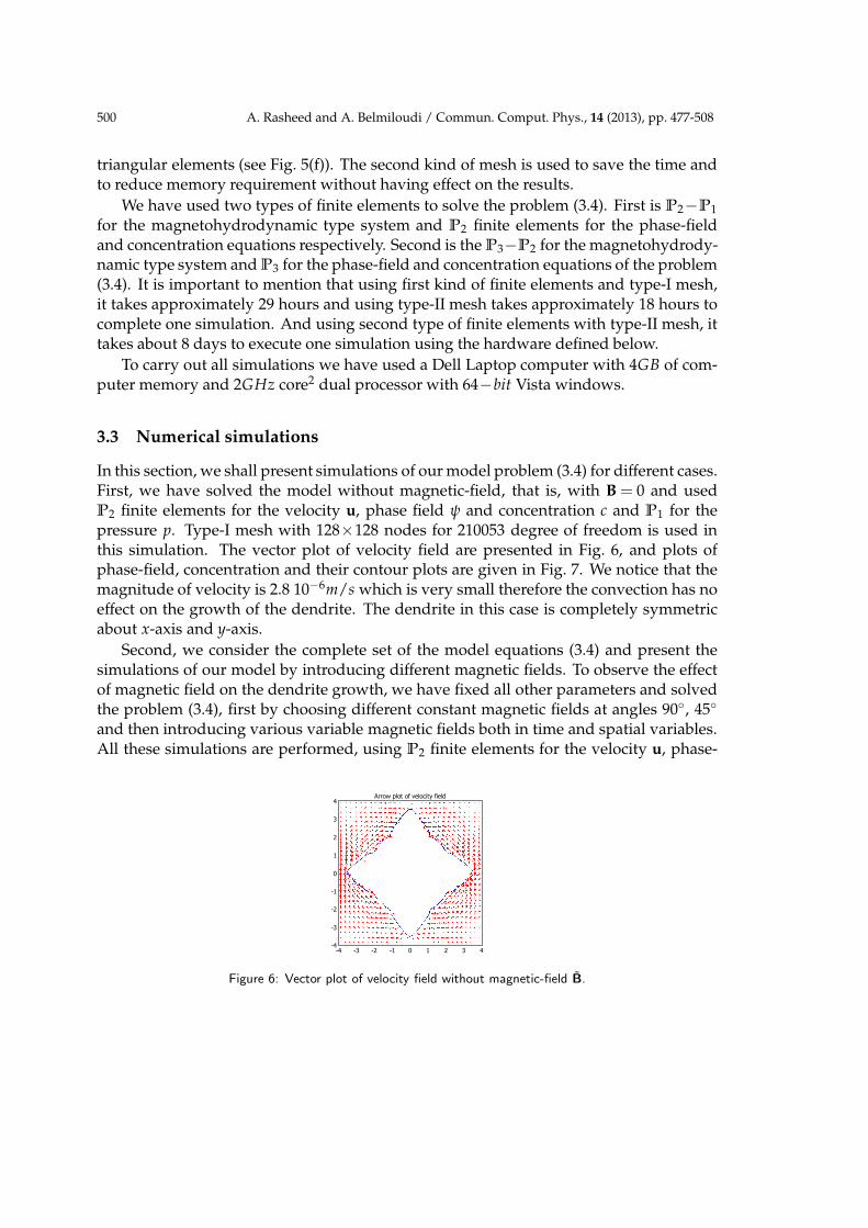
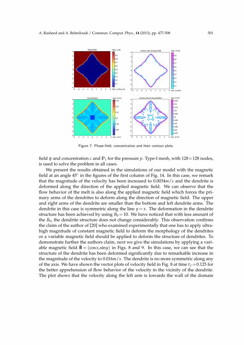
In this section, we shall present simulations of our model problem (3.4) for different cases.First, we have solved the model without magnetic-field, that is, with B = 0 and usedP2 finite elements for the velocity u, phase field ψ and concentration c and P1 for thepressure p. Type-I mesh with 128×128 nodes for 210053 degree of freedom is used inthis simulation. The vector plot of velocity field are presented in Fig. 6, and plots ofphase-field, concentration and their contour plots are given in Fig. 7. We notice that themagnitude of velocity is 2.8 10−6m/s which is very small therefore the convection has noeffect on the growth of the dendrite. The dendrite in this case is completely symmetricabout x-axis and y-axis.
Second, we consider the complete set of the model equations (3.4) and present thesimulations of our model by introducing different magnetic fields. To observe the effectof magnetic field on the dendrite growth, we have fixed all other parameters and solvedthe problem (3.4), first by choosing different constant magnetic fields at angles 90, 45
and then introducing various variable magnetic fields both in time and spatial variables.All these simulations are performed, using P2 finite elements for the velocity u, phase-
Figure 6: Vector plot of velocity field without magnetic-field B.
A. Rasheed and A. Belmiloudi / Commun. Comput. Phys., 14 (2013), pp. 477-508 501
Figure 7: Phase-field, concentration and their contour plots.
field ψ and concentration c and P1 for the pressure p. Type-I mesh, with 128×128 nodes,is used to solve the problem in all cases.
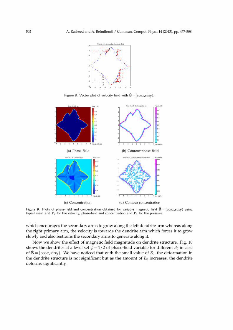
We present the results obtained in the simulations of our model with the magneticfield at an angle 45 in the figures of the first column of Fig. 14. In this case, we remarkthat the magnitude of the velocity has been increased to 0.0034m/s and the dendrite isdeformed along the direction of the applied magnetic field. We can observe that theflow behavior of the melt is also along the applied magnetic field which forces the pri-mary arms of the dendrites to deform along the direction of magnetic field. The upperand right arms of the dendrite are smaller than the bottom and left dendrite arms. Thedendrite in this case is symmetric along the line y= x. The deformation in the dendritestructure has been achieved by using B0 =10. We have noticed that with less amount ofthe B0, the dendrite structure does not change considerably. This observation confirmsthe claim of the author of [20] who examined experimentally that one has to apply ultra-high magnitude of constant magnetic field to deform the morphology of the dendritesor a variable magnetic field should be applied to deform the structure of dendrites. Todemonstrate further the authors claim, next we give the simulations by applying a vari-able magnetic field B = (cosx,siny) in Figs. 8 and 9. In this case, we can see that thestructure of the dendrite has been deformed significantly due to remarkable increase inthe magnitude of the velocity to 0.016m/s. The dendrite is no more symmetric along anyof the axis. We have shown the vector plots of velocity field in Fig. 8 at time t f =0.125 forthe better apprehension of flow behavior of the velocity in the vicinity of the dendrite.The plot shows that the velocity along the left arm is towards the wall of the domain
502 A. Rasheed and A. Belmiloudi / Commun. Comput. Phys., 14 (2013), pp. 477-508
Figure 8: Vector plot of velocity field with B=(cosx,siny).
(a) Phase-field (b) Contour phase-field
(c) Concentration (d) Contour concentration
Figure 9: Plots of phase-field and concentration obtained for variable magnetic field B= (cosx,siny) usingtype-I mesh and P2 for the velocity, phase-field and concentration and P1 for the pressure.
which encourages the secondary arms to grow along the left dendrite arm whereas alongthe right primary arm, the velocity is towards the dendrite arm which forces it to growslowly and also restrains the secondary arms to generate along it.
Now we show the effect of magnetic field magnitude on dendrite structure. Fig. 10shows the dendrites at a level set ψ= 1/2 of phase-field variable for different B0 in caseof B=(cosx,siny). We have noticed that with the small value of B0, the deformation inthe dendrite structure is not significant but as the amount of B0 increases, the dendritedeforms significantly.
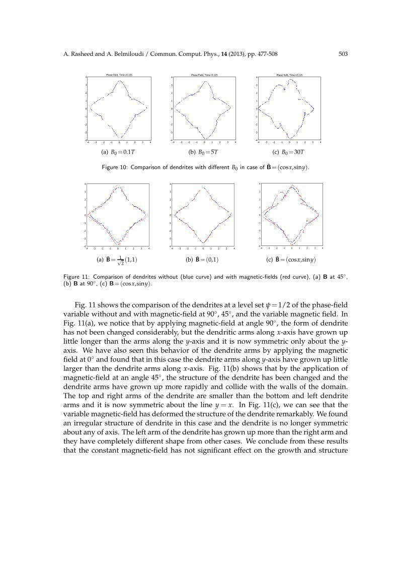
A. Rasheed and A. Belmiloudi / Commun. Comput. Phys., 14 (2013), pp. 477-508 503
(a) B0=0.1T (b) B0 =5T (c) B0=30T
Figure 10: Comparison of dendrites with different B0 in case of B=(cosx,siny).
(a) B= 1√2(1,1) (b) B=(0,1) (c) B=(cosx,siny)
Figure 11: Comparison of dendrites without (blue curve) and with magnetic-fields (red curve), (a) B at 45,(b) B at 90, (c) B=(cosx,siny).
Fig. 11 shows the comparison of the dendrites at a level set ψ=1/2 of the phase-fieldvariable without and with magnetic-field at 90, 45, and the variable magnetic field. InFig. 11(a), we notice that by applying magnetic-field at angle 90, the form of dendritehas not been changed considerably, but the dendritic arms along x-axis have grown uplittle longer than the arms along the y-axis and it is now symmetric only about the y-axis. We have also seen this behavior of the dendrite arms by applying the magneticfield at 0 and found that in this case the dendrite arms along y-axis have grown up littlelarger than the dendrite arms along x-axis. Fig. 11(b) shows that by the application ofmagnetic-field at an angle 45, the structure of the dendrite has been changed and thedendrite arms have grown up more rapidly and collide with the walls of the domain.The top and right arms of the dendrite are smaller than the bottom and left dendritearms and it is now symmetric about the line y = x. In Fig. 11(c), we can see that thevariable magnetic-field has deformed the structure of the dendrite remarkably. We foundan irregular structure of dendrite in this case and the dendrite is no longer symmetricabout any of axis. The left arm of the dendrite has grown up more than the right arm andthey have completely different shape from other cases. We conclude from these resultsthat the constant magnetic-field has not significant effect on the growth and structure
504 A. Rasheed and A. Belmiloudi / Commun. Comput. Phys., 14 (2013), pp. 477-508
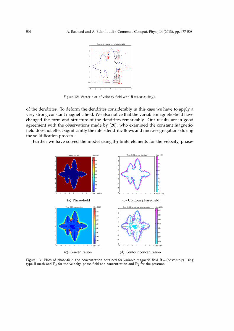
Figure 12: Vector plot of velocity field with B=(cosx,siny).
of the dendrites. To deform the dendrites considerably in this case we have to apply avery strong constant magnetic field. We also notice that the variable magnetic-field havechanged the form and structure of the dendrites remarkably. Our results are in goodagreement with the observations made by [20], who examined the constant magnetic-field does not effect significantly the inter-dendritic flows and micro-segregations duringthe solidification process.
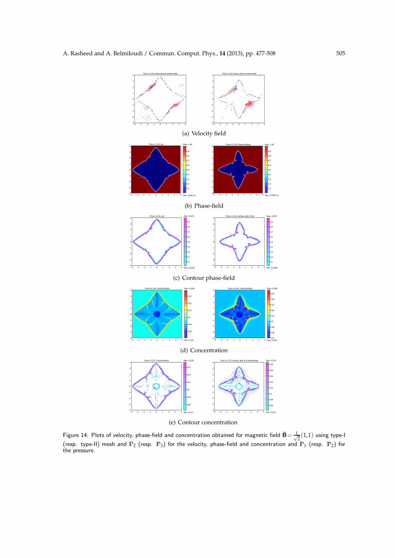
Further we have solved the model using P3 finite elements for the velocity, phase-
(a) Phase-field (b) Contour phase-field
(c) Concentration (d) Contour concentration
Figure 13: Plots of phase-field and concentration obtained for variable magnetic field B= (cosx,siny) usingtype-II mesh and P3 for the velocity, phase-field and concentration and P2 for the pressure.
A. Rasheed and A. Belmiloudi / Commun. Comput. Phys., 14 (2013), pp. 477-508 505
(a) Velocity field
(b) Phase-field
(c) Contour phase-field
(d) Concentration
(e) Contour concentration
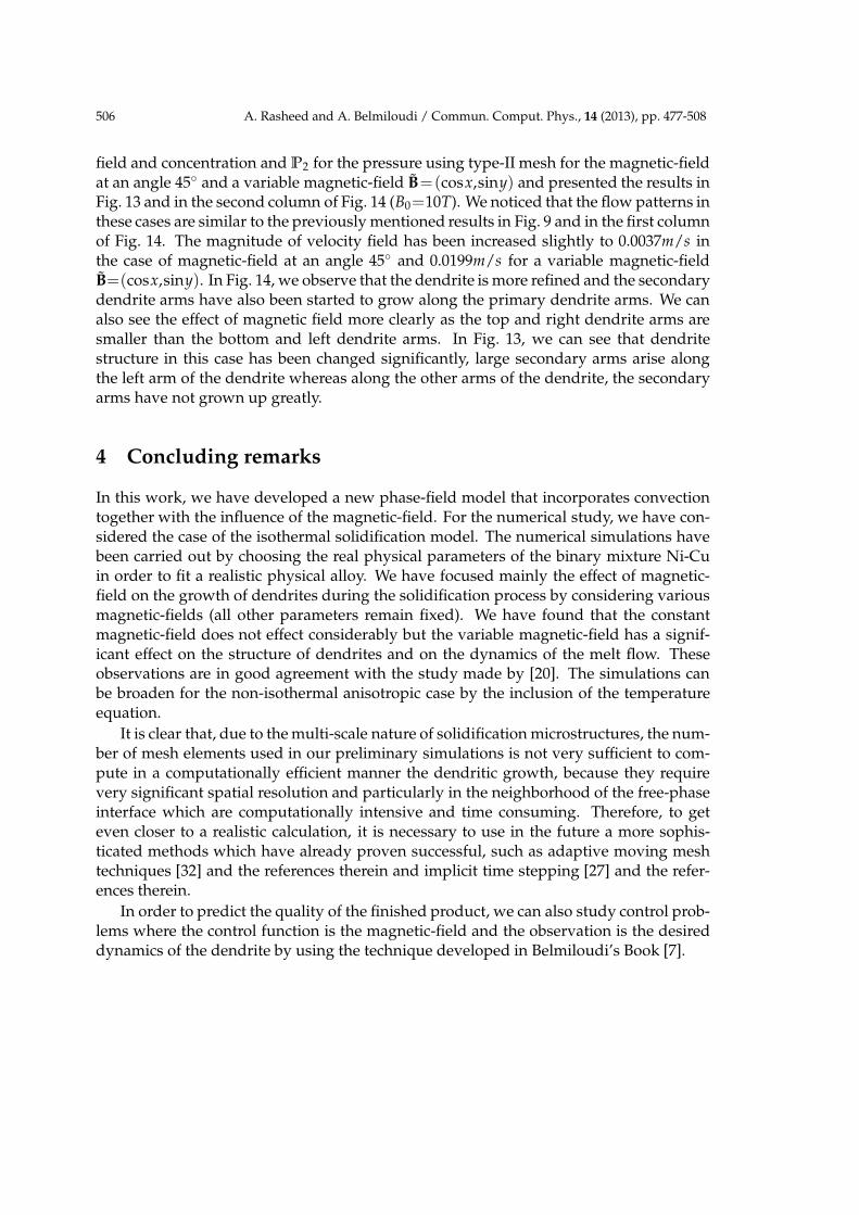
Figure 14: Plots of velocity, phase-field and concentration obtained for magnetic field B= 1√2(1,1) using type-I
(resp. type-II) mesh and P2 (resp. P3) for the velocity, phase-field and concentration and P1 (resp. P2) forthe pressure.
506 A. Rasheed and A. Belmiloudi / Commun. Comput. Phys., 14 (2013), pp. 477-508
field and concentration and P2 for the pressure using type-II mesh for the magnetic-fieldat an angle 45 and a variable magnetic-field B=(cosx,siny) and presented the results inFig. 13 and in the second column of Fig. 14 (B0=10T). We noticed that the flow patterns inthese cases are similar to the previously mentioned results in Fig. 9 and in the first columnof Fig. 14. The magnitude of velocity field has been increased slightly to 0.0037m/s inthe case of magnetic-field at an angle 45 and 0.0199m/s for a variable magnetic-fieldB=(cosx,siny). In Fig. 14, we observe that the dendrite is more refined and the secondarydendrite arms have also been started to grow along the primary dendrite arms. We canalso see the effect of magnetic field more clearly as the top and right dendrite arms aresmaller than the bottom and left dendrite arms. In Fig. 13, we can see that dendritestructure in this case has been changed significantly, large secondary arms arise alongthe left arm of the dendrite whereas along the other arms of the dendrite, the secondaryarms have not grown up greatly.
4 Concluding remarks
In this work, we have developed a new phase-field model that incorporates convectiontogether with the influence of the magnetic-field. For the numerical study, we have con-sidered the case of the isothermal solidification model. The numerical simulations havebeen carried out by choosing the real physical parameters of the binary mixture Ni-Cuin order to fit a realistic physical alloy. We have focused mainly the effect of magnetic-field on the growth of dendrites during the solidification process by considering variousmagnetic-fields (all other parameters remain fixed). We have found that the constantmagnetic-field does not effect considerably but the variable magnetic-field has a signif-icant effect on the structure of dendrites and on the dynamics of the melt flow. Theseobservations are in good agreement with the study made by [20]. The simulations canbe broaden for the non-isothermal anisotropic case by the inclusion of the temperatureequation.
It is clear that, due to the multi-scale nature of solidification microstructures, the num-ber of mesh elements used in our preliminary simulations is not very sufficient to com-pute in a computationally efficient manner the dendritic growth, because they requirevery significant spatial resolution and particularly in the neighborhood of the free-phaseinterface which are computationally intensive and time consuming. Therefore, to geteven closer to a realistic calculation, it is necessary to use in the future a more sophis-ticated methods which have already proven successful, such as adaptive moving meshtechniques [32] and the references therein and implicit time stepping [27] and the refer-ences therein.
In order to predict the quality of the finished product, we can also study control prob-lems where the control function is the magnetic-field and the observation is the desireddynamics of the dendrite by using the technique developed in Belmiloudi’s Book [7].
A. Rasheed and A. Belmiloudi / Commun. Comput. Phys., 14 (2013), pp. 477-508 507
Acknowledgments
The authors are grateful to the referees for many useful comments and suggestions whichhave improved the presentation of this paper.
References
[1] N. Al-Rawahi and G. Tryggvason, Numerical simulation of dendritic solidification withconvection: Two dimensional geometry, J. Comput. Phys., 180 (2002), 471-496.
[2] D.M. Anderson, G.B. McFadden and A.A. Wheeler, A phase-field model of solidificationwith convection, Physica D, 135 (2000), 175-194.
[3] E. Bansch and A. Schmidt, Simulation of dendritic crystal growth with thermal convection,EMS, Interfaces and Free Boundaries, 2 (2000), 95-115.
[4] A. Belmiloudi, Robin-type boundary control problems for the nonlinear Boussinesq typeequations, Journal of Mathematical Analysis and Applications, 273 (2002), 428-456.
[5] A. Belmiloudi, Robust and optimal control problems to a phase-field model for the solidi-fication of a binary alloy with a constant temperature, J. Dynamical and Control Systems,10 (2004), 453-499.
[6] A. Belmiloudi and J.P. Yvon, Robust control of a non-isothermal solidification model,WSEAS Transactions on systems, 4 (2005), 2291-2300.
[7] A. Belmiloudi, Stabilization, optimal and robust control: Theory and Applications in Bio-logical and Physical Systems, Springer-Verlag, London, Berlin, 2008.
[8] S. Bhattacharyya, T.W. Heo, K. Chang and L.Q. Chen, A spectral iterative method for thecomputation of effective properties of elastically inhomogeneous polycrystals, Commun.Comput. Phys., 11 (2012), 726-738.
[9] V. Galindo, G. Gerbeth, W.V. Ammon, E. Tomzig and J. Virbulis, Crystal growth melt flowprevious term control next term by means of magnetic fields, Energy Conv. Manage., 43(2002), 309-316.
[10] M. Grujicic, G. Cao and R.S. Millar, Computer modelling of the evolution of dendrite mi-crostructure in binary alloys during non-isotheraml solidification, J. Materials synthesisand processing, 10 (2002), 191-203.
[11] M. Gunzberger, E. Ozugurlu, J. Turner and H. Zhang, Controlling transport phenomena inthe Czochralski crystal growth process, J. Crystal Growth, 234 (2002), 47-62.
[12] H.B. Hadid, D. Henry and S. Kaddeche, Numerical study of convection in the horizontalBridgman configuration under the action of a constant magnetic field. Part 1. Two dimen-sional flow, J. Fluid Mech., 333 (1997), 23-56.
[13] B. Kaouil, M. Noureddine, R. Nassif and Y. Boughaleb, Phase-field modelling of dendriticgrowth behaviour towards the cooling/heating of pure nickel, Moroccan J. CondensedMatter, 6 (2005), 109-112.
[14] A. Karma and W.J. Rappel, Quantitative phase-field modeling of dendritic growth in twoand three dimensions, Physical Review E, 57 (1998), 4323-4349.
[15] D. Kessler, Modeling, Mathematical and numerical study of a solutal phase-field model,These, Lausanne EPFL, 2001.
[16] J. Kim, Phase-field models for multi-component fluid flows, Commun. Comput. Phys., 12(2012), 613-661.
508 A. Rasheed and A. Belmiloudi / Commun. Comput. Phys., 14 (2013), pp. 477-508
[17] P. Laurencot, Weak solutions to a phase-field model with non-constant thermal conductiv-ity, Quart. Appl. Math., 4 (1997), 739-760.
[18] M. Li, T. Takuya, N. Omura and K. Miwa, Effects of magnetic field and electric currenton the solidification of AZ91D magnesium alloys using an electromagnetic vibration tech-nique, J. of Alloys and Compounds, 487 (2009), 187-193.
[19] L.R. Petzold, A discription of DASSL: A differential/algebraic system solver, Scientificcomputing, IMACS Trans. Sci. Comput., (1983), 65-68.
[20] P.J. Prescott and F.P. Incropera, Magnetically damped convection during solidification of abinary metal alloy, Trans. ASME, 115 (1993), 302-310.
[21] A. Rasheed and A. Belmiloudi, An analysis of a phase-field model for isothermal binaryalloy solidification with convection under the influence of magnetic field, Journal of Math-ematical Analysis and Applications, 390 (2012), 244-273.
[22] J.C. Ramirez, C. Beckermann, A. Karma and H.J. Diepers, Phase-field modeling of binaryalloy solidification with couple heat and solute diffusion, Physical Review E, 69 (2004),(051607-1)-(051607-16).
[23] J.C. Ramirez and C. Beckermann, Examination of binary alloy free dendritic growth theo-ries with a phase-field model, Acta Materialia, 53 (2005), 1721-1736.
[24] J. Rappaz and J.F. Scheid, Existence of solutions to a phase-field model for the isothermalsolidification process of a binary alloy, Mathematical Methods in the Applied Sciences, 23(2000), 491-513.
[25] M. Rappaz and M. Rettenmayr, Simulation of solidification, Current Opinion in Solid Stateand Materials Science, 3 (1998), 275-282.
[26] J.K. Roplekar and J.A. Dantzig, A study of solidification with a rotating magnetic field, Int.J. Cast Met. Res., 14 (2001), 79-95.
[27] J. Rosam, P.K. Jimack and A.M. Mullis, A fully implicit, fully adaptive time and spacediscretisation method for phase-field simulation of binary alloy solidification, J. Comput.Phys., 225 (2007), 1271-1287.
[28] R. Sampath, The adjoint method for the design of directional binary alloy solidificationprocesses in the presence of a strong magnetic field, Thesis, Cornell University USA, 2001.
[29] T. Takaki, T. Fukuoka, Y. Tomita, Phase-field simulations during directional solidification ofa binary alloy using adaptive finite element method, J. Crystal Growth, 283 (2005), 263-278.
[30] X. Tong, C. Beckermann, A. Karma and Q. Li, Phase-field simulations of dendritic crystalgrowth in a forced flow, Physical Review E, 63 (2001), (061601-1)-(061601-16).
[31] Tonhardt R. and Amberg G., Simulation of natural convection effects on succinonitrile crys-tals, Physical Review E, 62 (2000), 828-836.
[32] H. Wang, R. Li and T. Tang, Efficient computation of dendritic growth with r-adaptive finiteelement methods, J. Comput. Physics, 227 (2008), 5984-6000.
[33] S.L. Wang, R.F. Sekerka, A.A. Wheeler, B.T. Murray, S.R. Coriell, R.J. Braun and G.B. Mc-Fadden, Thermodynamically-Consistent Phase-Field Models for Solidification, Physica D,69 (1993), 189-200.
[34] J.A. Warren and W.J. Boettinger, Prediction of dendritic growth and microsegregation pat-terns in a binary alloy using the phase-field method, Acta metall. mater, 43 (1995), 689-703.
[35] M. Watanabe, D. Vizman, J. Friedrich and G. Mueller, Large modification of crystal-meltinterface shape during Si crystal growth by using electromagnetic Czochralski method, J.Crystal Growth, 292 (2006), 252-256.
[36] A.A. Wheeler, W.J. Boettinger and G.B. McFadden, Phase-field model for isothermal phasetransitions in binary alloys, Physical Review A, 45 (1992), 7424-7439.