Embed Size (px)
Citation preview

Mathematics 13: Lecture 12Elementary Matrices and Finding Inverses
Dan Sloughter
Furman University
January 30, 2008
Dan Sloughter (Furman University) Mathematics 13: Lecture 12 January 30, 2008 1 / 24

Result from previous lecture
I The following statements are equivalent for an n × n matrix A:
I A is invertible.I The only solution to A~x = ~0 is the trivial solution ~x = ~0.I The reduced row-echelon form of A is In.I A~x = ~b has a solution for ~b in Rn.I There exists an n × n matrix C for which AC = In.
Dan Sloughter (Furman University) Mathematics 13: Lecture 12 January 30, 2008 2 / 24

Result from previous lecture
I The following statements are equivalent for an n × n matrix A:I A is invertible.
I The only solution to A~x = ~0 is the trivial solution ~x = ~0.I The reduced row-echelon form of A is In.I A~x = ~b has a solution for ~b in Rn.I There exists an n × n matrix C for which AC = In.
Dan Sloughter (Furman University) Mathematics 13: Lecture 12 January 30, 2008 2 / 24
Result from previous lecture
I The following statements are equivalent for an n × n matrix A:I A is invertible.I The only solution to A~x = ~0 is the trivial solution ~x = ~0.
I The reduced row-echelon form of A is In.I A~x = ~b has a solution for ~b in Rn.I There exists an n × n matrix C for which AC = In.
Dan Sloughter (Furman University) Mathematics 13: Lecture 12 January 30, 2008 2 / 24

Result from previous lecture
I The following statements are equivalent for an n × n matrix A:I A is invertible.I The only solution to A~x = ~0 is the trivial solution ~x = ~0.I The reduced row-echelon form of A is In.
I A~x = ~b has a solution for ~b in Rn.I There exists an n × n matrix C for which AC = In.
Dan Sloughter (Furman University) Mathematics 13: Lecture 12 January 30, 2008 2 / 24

Result from previous lecture
I The following statements are equivalent for an n × n matrix A:I A is invertible.I The only solution to A~x = ~0 is the trivial solution ~x = ~0.I The reduced row-echelon form of A is In.I A~x = ~b has a solution for ~b in Rn.
I There exists an n × n matrix C for which AC = In.
Dan Sloughter (Furman University) Mathematics 13: Lecture 12 January 30, 2008 2 / 24

Result from previous lecture
I The following statements are equivalent for an n × n matrix A:I A is invertible.I The only solution to A~x = ~0 is the trivial solution ~x = ~0.I The reduced row-echelon form of A is In.I A~x = ~b has a solution for ~b in Rn.I There exists an n × n matrix C for which AC = In.
Dan Sloughter (Furman University) Mathematics 13: Lecture 12 January 30, 2008 2 / 24
Computing an inverse
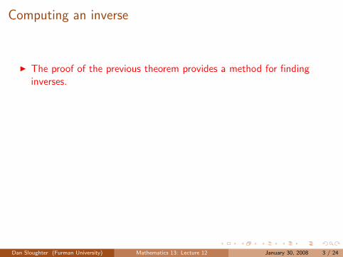
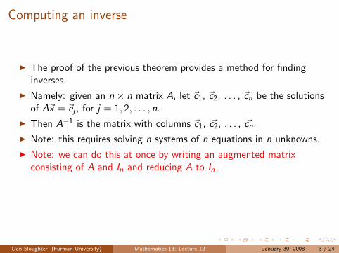
I The proof of the previous theorem provides a method for findinginverses.
I Namely: given an n × n matrix A, let ~c1, ~c2, . . . , ~cn be the solutionsof A~x = ~ej , for j = 1, 2, . . . , n.
I Then A−1 is the matrix with columns ~c1, ~c2, . . . , ~cn.
I Note: this requires solving n systems of n equations in n unknowns.
I Note: we can do this at once by writing an augmented matrixconsisting of A and In and reducing A to In.
I That is, the same row operations which take A to In take In to A−1.
Dan Sloughter (Furman University) Mathematics 13: Lecture 12 January 30, 2008 3 / 24

Computing an inverse
I The proof of the previous theorem provides a method for findinginverses.
I Namely: given an n × n matrix A, let ~c1, ~c2, . . . , ~cn be the solutionsof A~x = ~ej , for j = 1, 2, . . . , n.
I Then A−1 is the matrix with columns ~c1, ~c2, . . . , ~cn.
I Note: this requires solving n systems of n equations in n unknowns.
I Note: we can do this at once by writing an augmented matrixconsisting of A and In and reducing A to In.
I That is, the same row operations which take A to In take In to A−1.
Dan Sloughter (Furman University) Mathematics 13: Lecture 12 January 30, 2008 3 / 24
Example
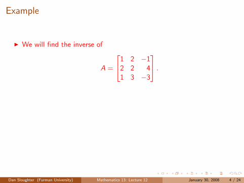
I We will find the inverse of
A =
1 2 −12 2 41 3 −3
.
I Using elementary row operations, we find1 2 −1 1 0 02 2 4 0 1 01 3 −3 0 0 1
−→1 2 −1 1 0 0
0 −2 6 −2 1 00 1 −2 −1 0 1
Dan Sloughter (Furman University) Mathematics 13: Lecture 12 January 30, 2008 4 / 24

Example
I We will find the inverse of
A =
1 2 −12 2 41 3 −3
.
I Using elementary row operations, we find1 2 −1 1 0 02 2 4 0 1 01 3 −3 0 0 1
−→1 2 −1 1 0 0
0 −2 6 −2 1 00 1 −2 −1 0 1
Dan Sloughter (Furman University) Mathematics 13: Lecture 12 January 30, 2008 4 / 24
Example (cont’d)
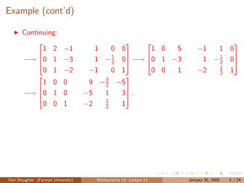
I Continuing:
−→
1 2 −1 1 0 0
0 1 −3 1 −12 0
0 1 −2 −1 0 1
−→1 0 5 −1 1 0
0 1 −3 1 −12 0
0 0 1 −2 12 1
−→
1 0 0 9 −32 −5
0 1 0 −5 1 3
0 0 1 −2 12 1
.
I Hence
A−1 =
9 −32 −5
−5 1 3
−2 12 1
.
Dan Sloughter (Furman University) Mathematics 13: Lecture 12 January 30, 2008 5 / 24

Example (cont’d)
I Continuing:
−→
1 2 −1 1 0 0
0 1 −3 1 −12 0
0 1 −2 −1 0 1
−→1 0 5 −1 1 0
0 1 −3 1 −12 0
0 0 1 −2 12 1
−→
1 0 0 9 −32 −5
0 1 0 −5 1 3
0 0 1 −2 12 1
.
I Hence
A−1 =
9 −32 −5
−5 1 3
−2 12 1
.
Dan Sloughter (Furman University) Mathematics 13: Lecture 12 January 30, 2008 5 / 24
Example
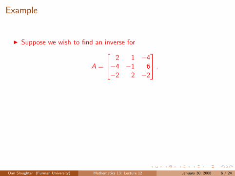
I Suppose we wish to find an inverse for
A =
2 1 −4−4 −1 6−2 2 −2
.
I Using elementary row operations, we find that 2 1 −4 1 0 0−4 −1 6 0 1 0−2 2 −2 0 0 1
−→2 1 −4 1 0 0
0 1 −2 2 1 00 3 −6 1 0 1
Dan Sloughter (Furman University) Mathematics 13: Lecture 12 January 30, 2008 6 / 24

Example
I Suppose we wish to find an inverse for
A =
2 1 −4−4 −1 6−2 2 −2
.
I Using elementary row operations, we find that 2 1 −4 1 0 0−4 −1 6 0 1 0−2 2 −2 0 0 1
−→2 1 −4 1 0 0
0 1 −2 2 1 00 3 −6 1 0 1
Dan Sloughter (Furman University) Mathematics 13: Lecture 12 January 30, 2008 6 / 24

Example (cont’d)
I Continuing, we have
−→
2 1 −4 1 0 00 1 −2 2 1 00 0 0 −5 −3 1
.
I Note: this shows that it is not possible to reduce A to I3 usingelementary row operations.
I It follows that A does not have an inverse.
Dan Sloughter (Furman University) Mathematics 13: Lecture 12 January 30, 2008 7 / 24

Inverses in Octave
I To find the inverse of
A =
1 2 3−1 0 1
4 2 1
,
we can either
I apply rref to the augmented matrix 1 2 3 1 0 0−1 0 1 0 1 0
4 2 1 0 0 1
,
I or use inv(A).
Dan Sloughter (Furman University) Mathematics 13: Lecture 12 January 30, 2008 8 / 24

Inverses in Octave
I To find the inverse of
A =
1 2 3−1 0 1
4 2 1
,
we can eitherI apply rref to the augmented matrix 1 2 3 1 0 0
−1 0 1 0 1 04 2 1 0 0 1
,
I or use inv(A).
Dan Sloughter (Furman University) Mathematics 13: Lecture 12 January 30, 2008 8 / 24

Inverses in Octave
I To find the inverse of
A =
1 2 3−1 0 1
4 2 1
,
we can eitherI apply rref to the augmented matrix 1 2 3 1 0 0
−1 0 1 0 1 04 2 1 0 0 1
,
I or use inv(A).
Dan Sloughter (Furman University) Mathematics 13: Lecture 12 January 30, 2008 8 / 24

Inverses in Octave (cont’d)
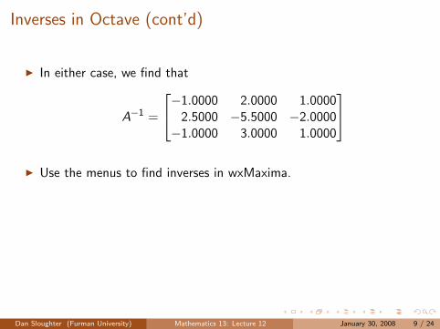
I In either case, we find that
A−1 =
−1.0000 2.0000 1.00002.5000 −5.5000 −2.0000−1.0000 3.0000 1.0000
I Use the menus to find inverses in wxMaxima.
I In wxMaxima, A.B multiplies the matrices A and B.
I In wxMaxima,
A^^3
raises A to the third power.
Dan Sloughter (Furman University) Mathematics 13: Lecture 12 January 30, 2008 9 / 24
Inverses in Octave (cont’d)
I In either case, we find that
A−1 =
−1.0000 2.0000 1.00002.5000 −5.5000 −2.0000−1.0000 3.0000 1.0000
I Use the menus to find inverses in wxMaxima.
I In wxMaxima, A.B multiplies the matrices A and B.
I In wxMaxima,
A^^3
raises A to the third power.
Dan Sloughter (Furman University) Mathematics 13: Lecture 12 January 30, 2008 9 / 24

Definition
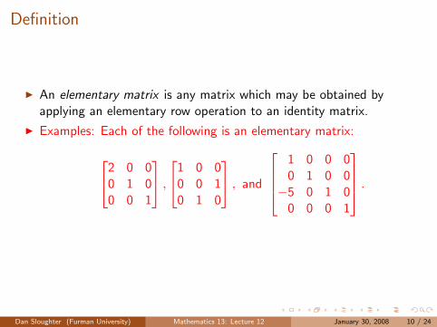
I An elementary matrix is any matrix which may be obtained byapplying an elementary row operation to an identity matrix.
I Examples: Each of the following is an elementary matrix:
2 0 00 1 00 0 1
,
1 0 00 0 10 1 0
, and
1 0 0 00 1 0 0−5 0 1 0
0 0 0 1
.
Dan Sloughter (Furman University) Mathematics 13: Lecture 12 January 30, 2008 10 / 24
Definition
I An elementary matrix is any matrix which may be obtained byapplying an elementary row operation to an identity matrix.
I Examples: Each of the following is an elementary matrix:
2 0 00 1 00 0 1
,
1 0 00 0 10 1 0
, and
1 0 0 00 1 0 0−5 0 1 0
0 0 0 1
.
Dan Sloughter (Furman University) Mathematics 13: Lecture 12 January 30, 2008 10 / 24

Example
I Let
A =
1 2 3 14 5 6 27 8 9 1
and E =
1 0 00 3 00 0 1
.
I Note: E is an elementary matrix obtained by multiplying the secondrow of I3 by 3.
I Note:
EA =
1 0 00 3 00 0 1
1 2 3 14 5 6 27 8 9 1
=
1 2 3 112 15 18 67 8 9 1
,
which is what we would obtain applying the same elementary rowoperation to A.
Dan Sloughter (Furman University) Mathematics 13: Lecture 12 January 30, 2008 11 / 24

Example (cont’d)
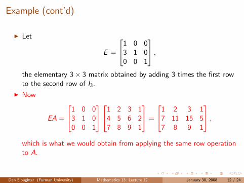
I Let
E =
1 0 03 1 00 0 1
,
the elementary 3× 3 matrix obtained by adding 3 times the first rowto the second row of I3.
I Now
EA =
1 0 03 1 00 0 1
1 2 3 14 5 6 27 8 9 1
=
1 2 3 17 11 15 57 8 9 1
,
which is what we would obtain from applying the same row operationto A.
Dan Sloughter (Furman University) Mathematics 13: Lecture 12 January 30, 2008 12 / 24
Example (cont’d)
I Let
E =
1 0 03 1 00 0 1
,
the elementary 3× 3 matrix obtained by adding 3 times the first rowto the second row of I3.
I Now
EA =
1 0 03 1 00 0 1
1 2 3 14 5 6 27 8 9 1
=
1 2 3 17 11 15 57 8 9 1
,
which is what we would obtain from applying the same row operationto A.
Dan Sloughter (Furman University) Mathematics 13: Lecture 12 January 30, 2008 12 / 24

Example (cont’d)
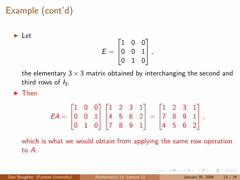
I Let
E =
1 0 00 0 10 1 0
,
the elementary 3× 3 matrix obtained by interchanging the second andthird rows of I3.
I Then
EA =
1 0 00 0 10 1 0
1 2 3 14 5 6 27 8 9 1
=
1 2 3 17 8 9 14 5 6 2
,
which is what we would obtain from applying the same row operationto A.
Dan Sloughter (Furman University) Mathematics 13: Lecture 12 January 30, 2008 13 / 24
Example (cont’d)
I Let
E =
1 0 00 0 10 1 0
,
the elementary 3× 3 matrix obtained by interchanging the second andthird rows of I3.
I Then
EA =
1 0 00 0 10 1 0
1 2 3 14 5 6 27 8 9 1
=
1 2 3 17 8 9 14 5 6 2
,
which is what we would obtain from applying the same row operationto A.
Dan Sloughter (Furman University) Mathematics 13: Lecture 12 January 30, 2008 13 / 24

Row operations
I Suppose an elementary row operation is performed on an m × nmatrix A to obtain the matrix B.
I Let E be the elementary matrix obtained by performing the same rowoperation on Im.
I Then B = EA.
Dan Sloughter (Furman University) Mathematics 13: Lecture 12 January 30, 2008 14 / 24

Row operations
I Suppose an elementary row operation is performed on an m × nmatrix A to obtain the matrix B.
I Let E be the elementary matrix obtained by performing the same rowoperation on Im.
I Then B = EA.
Dan Sloughter (Furman University) Mathematics 13: Lecture 12 January 30, 2008 14 / 24

Row operations
I Suppose an elementary row operation is performed on an m × nmatrix A to obtain the matrix B.
I Let E be the elementary matrix obtained by performing the same rowoperation on Im.
I Then B = EA.
Dan Sloughter (Furman University) Mathematics 13: Lecture 12 January 30, 2008 14 / 24

Inverses of elementary matrices
I Every elementary matrix E is invertible, and E−1 is itself anelementary matrix:
I If E multiplies a row by a nonzero scalar c , E−1 multiplies that samerow by 1
c .I If E multiplies row i by scalar c and adds it to row j , E−1 multiplies
row i by −c and adds it to row j .I If E interchanges rows i and j , E−1 interchanges rows i and j (and, so,
E = E−1).
Dan Sloughter (Furman University) Mathematics 13: Lecture 12 January 30, 2008 15 / 24

Inverses of elementary matrices
I Every elementary matrix E is invertible, and E−1 is itself anelementary matrix:
I If E multiplies a row by a nonzero scalar c , E−1 multiplies that samerow by 1
c .
I If E multiplies row i by scalar c and adds it to row j , E−1 multipliesrow i by −c and adds it to row j .
I If E interchanges rows i and j , E−1 interchanges rows i and j (and, so,E = E−1).
Dan Sloughter (Furman University) Mathematics 13: Lecture 12 January 30, 2008 15 / 24

Inverses of elementary matrices
I Every elementary matrix E is invertible, and E−1 is itself anelementary matrix:
I If E multiplies a row by a nonzero scalar c , E−1 multiplies that samerow by 1
c .I If E multiplies row i by scalar c and adds it to row j , E−1 multiplies
row i by −c and adds it to row j .
I If E interchanges rows i and j , E−1 interchanges rows i and j (and, so,E = E−1).
Dan Sloughter (Furman University) Mathematics 13: Lecture 12 January 30, 2008 15 / 24

Inverses of elementary matrices
I Every elementary matrix E is invertible, and E−1 is itself anelementary matrix:
I If E multiplies a row by a nonzero scalar c , E−1 multiplies that samerow by 1
c .I If E multiplies row i by scalar c and adds it to row j , E−1 multiplies
row i by −c and adds it to row j .I If E interchanges rows i and j , E−1 interchanges rows i and j (and, so,
E = E−1).
Dan Sloughter (Furman University) Mathematics 13: Lecture 12 January 30, 2008 15 / 24

Theorem
I Suppose an m × n matrix A is reducible to an m × n matrix B by aseries of elementary row operations. Then:
I B = EkEk−1 · · ·E1A, where E1, E2, . . . , Ek are elementary matrices.I B = UA for some invertible matrix U.I U is the matrix obtained from Im by performing the row operations on
Im which reduce A to B.
Dan Sloughter (Furman University) Mathematics 13: Lecture 12 January 30, 2008 16 / 24

Theorem
I Suppose an m × n matrix A is reducible to an m × n matrix B by aseries of elementary row operations. Then:
I B = EkEk−1 · · ·E1A, where E1, E2, . . . , Ek are elementary matrices.
I B = UA for some invertible matrix U.I U is the matrix obtained from Im by performing the row operations on
Im which reduce A to B.
Dan Sloughter (Furman University) Mathematics 13: Lecture 12 January 30, 2008 16 / 24

Theorem
I Suppose an m × n matrix A is reducible to an m × n matrix B by aseries of elementary row operations. Then:
I B = EkEk−1 · · ·E1A, where E1, E2, . . . , Ek are elementary matrices.I B = UA for some invertible matrix U.
I U is the matrix obtained from Im by performing the row operations onIm which reduce A to B.
Dan Sloughter (Furman University) Mathematics 13: Lecture 12 January 30, 2008 16 / 24

Theorem
I Suppose an m × n matrix A is reducible to an m × n matrix B by aseries of elementary row operations. Then:
I B = EkEk−1 · · ·E1A, where E1, E2, . . . , Ek are elementary matrices.I B = UA for some invertible matrix U.I U is the matrix obtained from Im by performing the row operations on
Im which reduce A to B.
Dan Sloughter (Furman University) Mathematics 13: Lecture 12 January 30, 2008 16 / 24

Example
I Let
A =
2 −1 4 61 2 1 25 0 9 14
.
I Applying row reduction, we have2 −1 4 6 1 0 01 2 1 2 0 1 05 0 9 14 0 0 1
−→1 2 1 2 0 1 0
2 −1 4 6 1 0 05 0 9 14 0 0 1
Dan Sloughter (Furman University) Mathematics 13: Lecture 12 January 30, 2008 17 / 24

Example
I Let
A =
2 −1 4 61 2 1 25 0 9 14
.
I Applying row reduction, we have2 −1 4 6 1 0 01 2 1 2 0 1 05 0 9 14 0 0 1
−→1 2 1 2 0 1 0
2 −1 4 6 1 0 05 0 9 14 0 0 1
Dan Sloughter (Furman University) Mathematics 13: Lecture 12 January 30, 2008 17 / 24

Example (cont’d)
I Continuing,
−→
1 2 1 2 0 1 00 −5 2 2 1 −2 00 −10 4 4 0 −5 1
−→
1 2 1 2 0 1 0
0 1 −25 −2
5 −15
25 0
0 −10 4 4 0 −5 1
−→
1 0 95
145
25
15 0
0 1 −25 −2
5 −15
25 0
0 0 0 0 −2 −1 1
.
Dan Sloughter (Furman University) Mathematics 13: Lecture 12 January 30, 2008 18 / 24

Example (cont’d)
I Hence if
B =
1 0 95
145
0 1 −25 −2
5
0 0 0 0
,
the reduced row-echelon form of A, and
U =
25
15 0
−15
25 0
−2 −1 1
,
then U is invertible and B = UA.
Dan Sloughter (Furman University) Mathematics 13: Lecture 12 January 30, 2008 19 / 24

Example (cont’d)
I Note: U is not unique.
I For example, using Octave to perform row reductions to reducedrow-echelon form, we obtain
V =
0.00000 0.00000 0.200000.00000 0.50000 −0.100001.00000 0.50000 −0.50000
with the property that V is invertible and B = VA.
I In particular, this shows that we may have UA = VA and yet U 6= V .
Dan Sloughter (Furman University) Mathematics 13: Lecture 12 January 30, 2008 20 / 24
Theorem
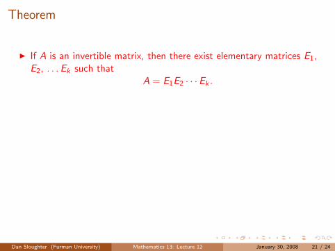
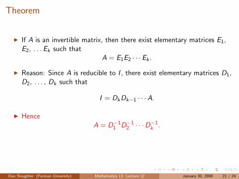
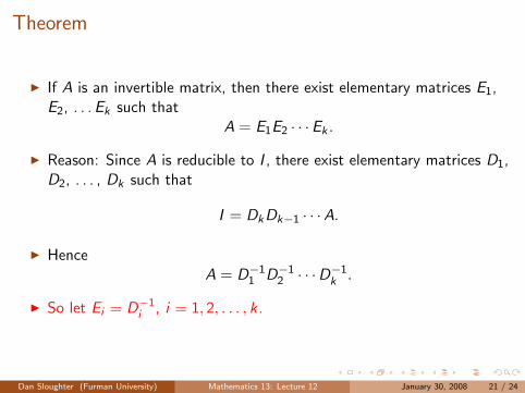
I If A is an invertible matrix, then there exist elementary matrices E1,E2, . . . Ek such that
A = E1E2 · · ·Ek .
I Reason: Since A is reducible to I , there exist elementary matrices D1,D2, . . . , Dk such that
I = DkDk−1 · · ·A.
I HenceA = D−1
1 D−12 · · ·D
−1k .
I So let Ei = D−1i , i = 1, 2, . . . , k .
Dan Sloughter (Furman University) Mathematics 13: Lecture 12 January 30, 2008 21 / 24

Theorem
I If A is an invertible matrix, then there exist elementary matrices E1,E2, . . . Ek such that
A = E1E2 · · ·Ek .
I Reason: Since A is reducible to I , there exist elementary matrices D1,D2, . . . , Dk such that
I = DkDk−1 · · ·A.
I HenceA = D−1
1 D−12 · · ·D
−1k .
I So let Ei = D−1i , i = 1, 2, . . . , k .
Dan Sloughter (Furman University) Mathematics 13: Lecture 12 January 30, 2008 21 / 24

Example
I If
A =
[3 21 −1
],
then I2 = D4D3D2D1A, where
D1 =
[0 11 0
], D2 =
[1 0−3 1
], D3 =
[1 00 1
5
], and D4 =
[1 10 1
].
Dan Sloughter (Furman University) Mathematics 13: Lecture 12 January 30, 2008 22 / 24
Example (cont’d)
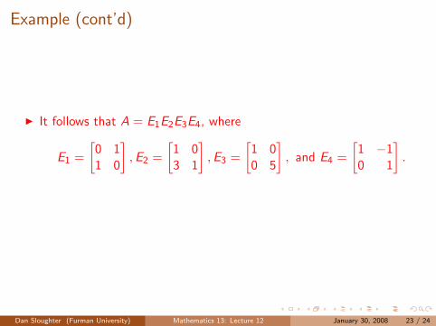
I It follows that A = E1E2E3E4, where
E1 =
[0 11 0
], E2 =
[1 03 1
], E3 =
[1 00 5
], and E4 =
[1 −10 1
].
Dan Sloughter (Furman University) Mathematics 13: Lecture 12 January 30, 2008 23 / 24

Theorem
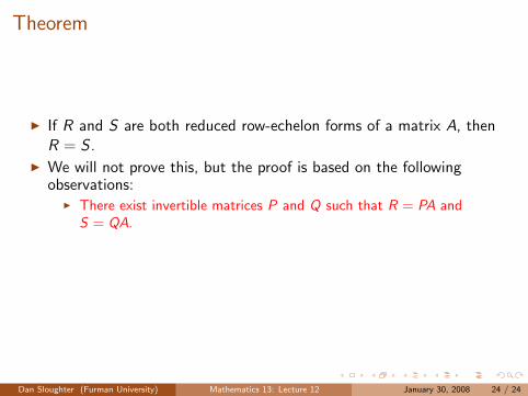
I If R and S are both reduced row-echelon forms of a matrix A, thenR = S .
I We will not prove this, but the proof is based on the followingobservations:
I There exist invertible matrices P and Q such that R = PA andS = QA.
I Hence A = Q−1S and A = P−1R, so S = QP−1R.I That is, S = UR for some invertible matrix U.
Dan Sloughter (Furman University) Mathematics 13: Lecture 12 January 30, 2008 24 / 24

Theorem
I If R and S are both reduced row-echelon forms of a matrix A, thenR = S .
I We will not prove this, but the proof is based on the followingobservations:
I There exist invertible matrices P and Q such that R = PA andS = QA.
I Hence A = Q−1S and A = P−1R, so S = QP−1R.I That is, S = UR for some invertible matrix U.
Dan Sloughter (Furman University) Mathematics 13: Lecture 12 January 30, 2008 24 / 24

Theorem
I If R and S are both reduced row-echelon forms of a matrix A, thenR = S .
I We will not prove this, but the proof is based on the followingobservations:
I There exist invertible matrices P and Q such that R = PA andS = QA.
I Hence A = Q−1S and A = P−1R, so S = QP−1R.
I That is, S = UR for some invertible matrix U.
Dan Sloughter (Furman University) Mathematics 13: Lecture 12 January 30, 2008 24 / 24

Theorem
I If R and S are both reduced row-echelon forms of a matrix A, thenR = S .
I We will not prove this, but the proof is based on the followingobservations:
I There exist invertible matrices P and Q such that R = PA andS = QA.
I Hence A = Q−1S and A = P−1R, so S = QP−1R.I That is, S = UR for some invertible matrix U.
Dan Sloughter (Furman University) Mathematics 13: Lecture 12 January 30, 2008 24 / 24


![[PPT]PENERAPAN EKONOMIme131.ilearning.me/.../1671/2015/02/math13.-INTEGRAL.ppt · Web viewINTEGRAL Integral tertentu digunakan untuk menghitung luas area yang terletak di antara kurva](https://img.pdfslide.net/doc/110x75/5af52e577f8b9ae9488d1d29/pptpenerapan-viewintegral-integral-tertentu-digunakan-untuk-menghitung-luas-area.jpg)