Embed Size (px)
Citation preview
Mathematics 22: Lecture 1Introduction
Dan Sloughter
Furman University
January 3, 2008
Dan Sloughter (Furman University) Mathematics 22: Lecture 1 January 3, 2008 1 / 16
Course information
I Course information is available at:http://math.furman.edu/~dcs/dokuwiki/
Dan Sloughter (Furman University) Mathematics 22: Lecture 1 January 3, 2008 2 / 16
Octave and Maxima
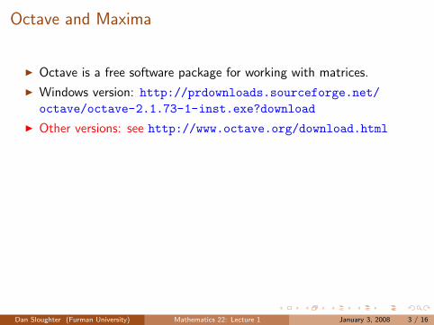
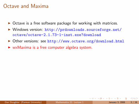
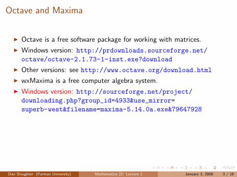
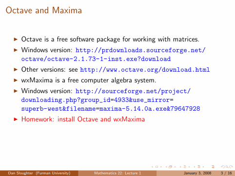
I Octave is a free software package for working with matrices.
I Windows version: http://prdownloads.sourceforge.net/octave/octave-2.1.73-1-inst.exe?download
I Other versions: see http://www.octave.org/download.html
I wxMaxima is a free computer algebra system.
I Windows version: http://sourceforge.net/project/downloading.php?group_id=4933&use_mirror=superb-west&filename=maxima-5.14.0a.exe&79647928
I Homework: install Octave and wxMaxima
I If you cannot install Octave and/or wxMaxima, see me about usingan account in the Mathematics Department computer lab.
Dan Sloughter (Furman University) Mathematics 22: Lecture 1 January 3, 2008 3 / 16
Octave and Maxima
I Octave is a free software package for working with matrices.
I Windows version: http://prdownloads.sourceforge.net/octave/octave-2.1.73-1-inst.exe?download
I Other versions: see http://www.octave.org/download.html
I wxMaxima is a free computer algebra system.
I Windows version: http://sourceforge.net/project/downloading.php?group_id=4933&use_mirror=superb-west&filename=maxima-5.14.0a.exe&79647928
I Homework: install Octave and wxMaxima
I If you cannot install Octave and/or wxMaxima, see me about usingan account in the Mathematics Department computer lab.
Dan Sloughter (Furman University) Mathematics 22: Lecture 1 January 3, 2008 3 / 16
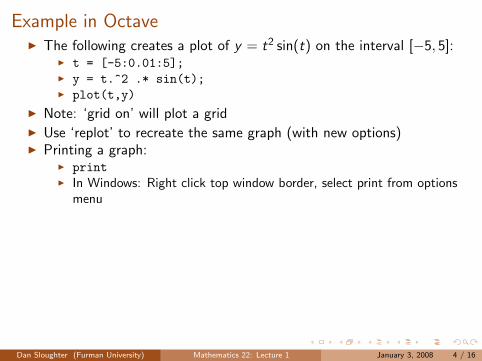
Example in OctaveI The following creates a plot of y = t2 sin(t) on the interval [−5, 5]:
I t = [-5:0.01:5];I y = t.^2 .* sin(t);I plot(t,y)
I Note: ‘grid on’ will plot a gridI Use ‘replot’ to recreate the same graph (with new options)I Printing a graph:
I printI In Windows: Right click top window border, select print from options
menuI Saving a graph:
I gset terminal png;I gset output "filename.png";I replot;
I To reset the terminal in Windows for plotting to the screen:I gset terminal win
I To reset the terminal in the lab for plotting to the screen:I gset terminal x11
Dan Sloughter (Furman University) Mathematics 22: Lecture 1 January 3, 2008 4 / 16
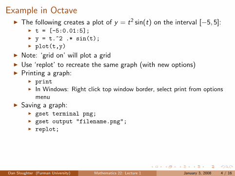
Example in OctaveI The following creates a plot of y = t2 sin(t) on the interval [−5, 5]:
I t = [-5:0.01:5];I y = t.^2 .* sin(t);I plot(t,y)
I Note: ‘grid on’ will plot a grid
I Use ‘replot’ to recreate the same graph (with new options)I Printing a graph:
I printI In Windows: Right click top window border, select print from options
menuI Saving a graph:
I gset terminal png;I gset output "filename.png";I replot;
I To reset the terminal in Windows for plotting to the screen:I gset terminal win
I To reset the terminal in the lab for plotting to the screen:I gset terminal x11
Dan Sloughter (Furman University) Mathematics 22: Lecture 1 January 3, 2008 4 / 16
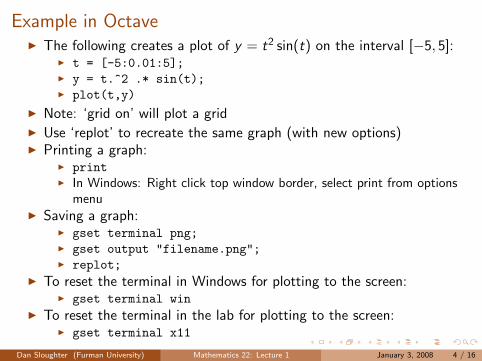
Example in OctaveI The following creates a plot of y = t2 sin(t) on the interval [−5, 5]:
I t = [-5:0.01:5];I y = t.^2 .* sin(t);I plot(t,y)
I Note: ‘grid on’ will plot a gridI Use ‘replot’ to recreate the same graph (with new options)
I Printing a graph:I printI In Windows: Right click top window border, select print from options
menuI Saving a graph:
I gset terminal png;I gset output "filename.png";I replot;
I To reset the terminal in Windows for plotting to the screen:I gset terminal win
I To reset the terminal in the lab for plotting to the screen:I gset terminal x11
Dan Sloughter (Furman University) Mathematics 22: Lecture 1 January 3, 2008 4 / 16
Example in OctaveI The following creates a plot of y = t2 sin(t) on the interval [−5, 5]:
I t = [-5:0.01:5];I y = t.^2 .* sin(t);I plot(t,y)
I Note: ‘grid on’ will plot a gridI Use ‘replot’ to recreate the same graph (with new options)I Printing a graph:
I printI In Windows: Right click top window border, select print from options
menu
I Saving a graph:I gset terminal png;I gset output "filename.png";I replot;
I To reset the terminal in Windows for plotting to the screen:I gset terminal win
I To reset the terminal in the lab for plotting to the screen:I gset terminal x11
Dan Sloughter (Furman University) Mathematics 22: Lecture 1 January 3, 2008 4 / 16
Example in OctaveI The following creates a plot of y = t2 sin(t) on the interval [−5, 5]:
I t = [-5:0.01:5];I y = t.^2 .* sin(t);I plot(t,y)
I Note: ‘grid on’ will plot a gridI Use ‘replot’ to recreate the same graph (with new options)I Printing a graph:
I printI In Windows: Right click top window border, select print from options
menuI Saving a graph:
I gset terminal png;I gset output "filename.png";I replot;
I To reset the terminal in Windows for plotting to the screen:I gset terminal win
I To reset the terminal in the lab for plotting to the screen:I gset terminal x11
Dan Sloughter (Furman University) Mathematics 22: Lecture 1 January 3, 2008 4 / 16
Example in OctaveI The following creates a plot of y = t2 sin(t) on the interval [−5, 5]:
I t = [-5:0.01:5];I y = t.^2 .* sin(t);I plot(t,y)
I Note: ‘grid on’ will plot a gridI Use ‘replot’ to recreate the same graph (with new options)I Printing a graph:
I printI In Windows: Right click top window border, select print from options
menuI Saving a graph:
I gset terminal png;I gset output "filename.png";I replot;
I To reset the terminal in Windows for plotting to the screen:I gset terminal win
I To reset the terminal in the lab for plotting to the screen:I gset terminal x11
Dan Sloughter (Furman University) Mathematics 22: Lecture 1 January 3, 2008 4 / 16
Example in Octave (cont’d)
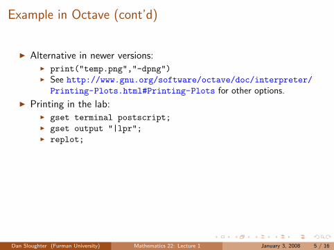
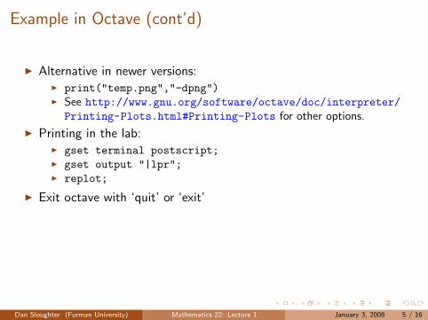
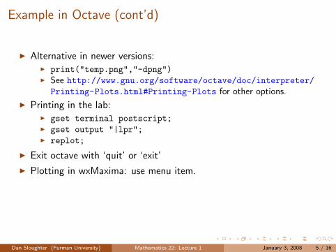
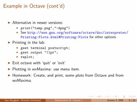
I Alternative in newer versions:I print("temp.png","-dpng")
I See http://www.gnu.org/software/octave/doc/interpreter/Printing-Plots.html#Printing-Plots for other options.
I Printing in the lab:I gset terminal postscript;I gset output "|lpr";I replot;
I Exit octave with ‘quit’ or ‘exit’
I Plotting in wxMaxima: use menu item.
I Homework: Create, and print, some plots from Octave and fromwxMaxima.
Dan Sloughter (Furman University) Mathematics 22: Lecture 1 January 3, 2008 5 / 16
Example in Octave (cont’d)
I Alternative in newer versions:I print("temp.png","-dpng")I See http://www.gnu.org/software/octave/doc/interpreter/
Printing-Plots.html#Printing-Plots for other options.
I Printing in the lab:I gset terminal postscript;I gset output "|lpr";I replot;
I Exit octave with ‘quit’ or ‘exit’
I Plotting in wxMaxima: use menu item.
I Homework: Create, and print, some plots from Octave and fromwxMaxima.
Dan Sloughter (Furman University) Mathematics 22: Lecture 1 January 3, 2008 5 / 16
Some terminology
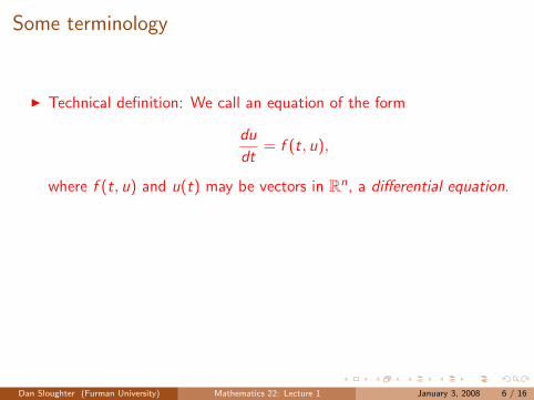
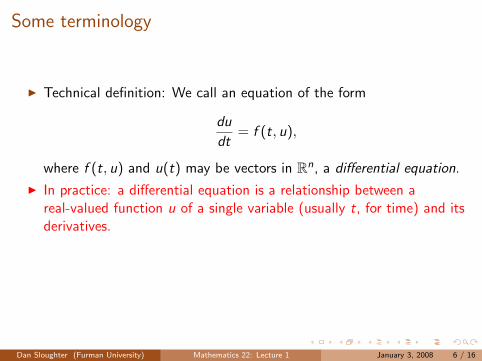
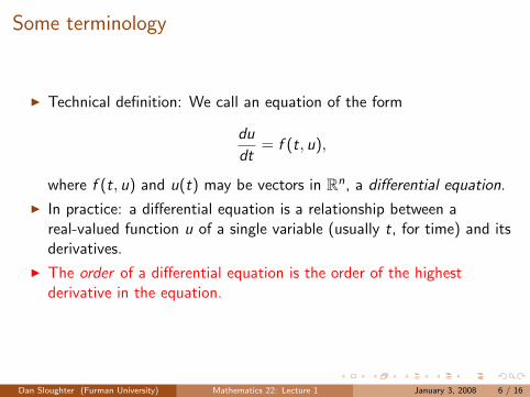
I Technical definition: We call an equation of the form
du
dt= f (t, u),
where f (t, u) and u(t) may be vectors in Rn, a differential equation.
I In practice: a differential equation is a relationship between areal-valued function u of a single variable (usually t, for time) and itsderivatives.
I The order of a differential equation is the order of the highestderivative in the equation.
Dan Sloughter (Furman University) Mathematics 22: Lecture 1 January 3, 2008 6 / 16
Some terminology
I Technical definition: We call an equation of the form
du
dt= f (t, u),
where f (t, u) and u(t) may be vectors in Rn, a differential equation.
I In practice: a differential equation is a relationship between areal-valued function u of a single variable (usually t, for time) and itsderivatives.
I The order of a differential equation is the order of the highestderivative in the equation.
Dan Sloughter (Furman University) Mathematics 22: Lecture 1 January 3, 2008 6 / 16
Examples
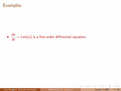
Idu
dt= t sin(u) is a first-order differential equation.
Id2u
dt2+ t2 du
dt+ cos(u) = cos(3t) is a second-order differential equation.
Dan Sloughter (Furman University) Mathematics 22: Lecture 1 January 3, 2008 7 / 16
Examples
Idu
dt= t sin(u) is a first-order differential equation.
Id2u
dt2+ t2 du
dt+ cos(u) = cos(3t) is a second-order differential equation.
Dan Sloughter (Furman University) Mathematics 22: Lecture 1 January 3, 2008 7 / 16
Solutions
I A solution of a differential equation is a continuous function which,with its derivatives, satisfies the relationship specified in the equation.
I Example:
I u = 4 cos(2t)− 3 sin(2t) is a solution to the equation
d2u
dt2= −4u.
I Verification:
d2u
dt2= −16 cos(2t) + 12 sin(2t) = −4(4 cos(2t)− 3 sin(2t)) = −4u.
I Note: this solution is not unique.I For example, both u = −8 sin(2t) and u = 23 cos(2t) are solutions as
well.
Dan Sloughter (Furman University) Mathematics 22: Lecture 1 January 3, 2008 8 / 16
Solutions
I A solution of a differential equation is a continuous function which,with its derivatives, satisfies the relationship specified in the equation.
I Example:I u = 4 cos(2t)− 3 sin(2t) is a solution to the equation
d2u
dt2= −4u.
I Verification:
d2u
dt2= −16 cos(2t) + 12 sin(2t) = −4(4 cos(2t)− 3 sin(2t)) = −4u.
I Note: this solution is not unique.
I For example, both u = −8 sin(2t) and u = 23 cos(2t) are solutions aswell.
Dan Sloughter (Furman University) Mathematics 22: Lecture 1 January 3, 2008 8 / 16
Solutions
I A solution of a differential equation is a continuous function which,with its derivatives, satisfies the relationship specified in the equation.
I Example:I u = 4 cos(2t)− 3 sin(2t) is a solution to the equation
d2u
dt2= −4u.
I Verification:
d2u
dt2= −16 cos(2t) + 12 sin(2t) = −4(4 cos(2t)− 3 sin(2t)) = −4u.
I Note: this solution is not unique.I For example, both u = −8 sin(2t) and u = 23 cos(2t) are solutions as
well.
Dan Sloughter (Furman University) Mathematics 22: Lecture 1 January 3, 2008 8 / 16
Some terminology
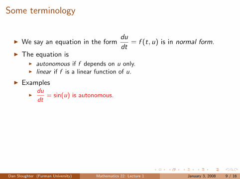
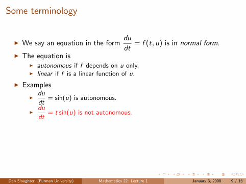
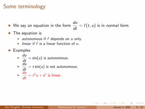
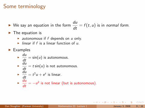
I We say an equation in the formdu
dt= f (t, u) is in normal form.
I The equation is
I autonomous if f depends on u only.I linear if f is a linear function of u.
I Examples
Idu
dt= sin(u) is autonomous.
Idu
dt= t sin(u) is not autonomous.
Idu
dt= t2u + et is linear.
Idu
dt= −u2 is not linear (but is autonomous).
Dan Sloughter (Furman University) Mathematics 22: Lecture 1 January 3, 2008 9 / 16
Some terminology
I We say an equation in the formdu
dt= f (t, u) is in normal form.
I The equation isI autonomous if f depends on u only.
I linear if f is a linear function of u.
I Examples
Idu
dt= sin(u) is autonomous.
Idu
dt= t sin(u) is not autonomous.
Idu
dt= t2u + et is linear.
Idu
dt= −u2 is not linear (but is autonomous).
Dan Sloughter (Furman University) Mathematics 22: Lecture 1 January 3, 2008 9 / 16
Some terminology
I We say an equation in the formdu
dt= f (t, u) is in normal form.
I The equation isI autonomous if f depends on u only.I linear if f is a linear function of u.
I Examples
Idu
dt= sin(u) is autonomous.
Idu
dt= t sin(u) is not autonomous.
Idu
dt= t2u + et is linear.
Idu
dt= −u2 is not linear (but is autonomous).
Dan Sloughter (Furman University) Mathematics 22: Lecture 1 January 3, 2008 9 / 16
General and particular solutions
I Example: u = cet is a solution ofdu
dt= u for any value of c .
I Moreover, if u is a solution ofdu
dt= u, then u = cet for some value of
c .
I We call u = cet a one-parameter family of solutions to the equationdu
dt= u.
I Moreover, this family of solutions is the general solution ofdu
dt= u.
I Note: If we further require that u(0) = 10, then we find thatu(t) = 10et is the unique solution to the initial value problem
du
dt= u,
u(0) = 10.
I We call u(t) = 10et a particular solution ofdu
dt= u.
Dan Sloughter (Furman University) Mathematics 22: Lecture 1 January 3, 2008 10 / 16
Solutions
I Example: The initial value problemdu
dt=√
u,
u(0) = −10
has no solutions.
I Example: The initial value problemdu
dt= u
23 ,
u(0) = 0
has an infinite number of solutions, including u ≡ 0 and u = 127 t3.
Dan Sloughter (Furman University) Mathematics 22: Lecture 1 January 3, 2008 11 / 16
Solutions
I Example: The initial value problemdu
dt=√
u,
u(0) = −10
has no solutions.
I Example: The initial value problemdu
dt= u
23 ,
u(0) = 0
has an infinite number of solutions, including u ≡ 0 and u = 127 t3.
Dan Sloughter (Furman University) Mathematics 22: Lecture 1 January 3, 2008 11 / 16
Partial derivatives
I If f is a function of both t and u, then ft denotes the derivative of fconsidered as a function of t alone, and fu denotes the derivative of fas a function of u alone.
I Example: If f (t, u) = t2 + 2tu + u3, then
ft(t, u) = 2t + 2u and fu(t, u) = 2t + 3u2.
I We call ft and fu the partial derivatives of f with respect to t and u,respectively.
I Notation: we also write
∂
∂tf (t, u) = ft(t, u) and
∂
∂uf (t, u) = fu(t, u).
Dan Sloughter (Furman University) Mathematics 22: Lecture 1 January 3, 2008 12 / 16
Existence and uniqueness
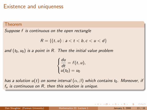
Theorem
Suppose f is continuous on the open rectangle
R = {(t, u) : a < t < b, c < u < d}
and (t0, u0) is a point in R. Then the initial value problemdu
dt= f (t, u),
u(t0) = u0
has a solution u(t) on some interval (α, β) which contains t0. Moreover, iffu is continuous on R, then this solution is unique.
Dan Sloughter (Furman University) Mathematics 22: Lecture 1 January 3, 2008 13 / 16
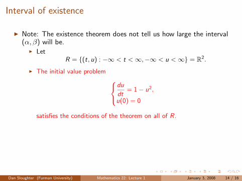
Interval of existence
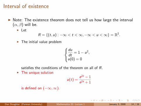
I Note: The existence theorem does not tell us how large the interval(α, β) will be.
I LetR = {(t, u) : −∞ < t <∞,−∞ < u <∞} = R2.
I The initial value problem du
dt= 1− u2,
u(0) = 0
satisfies the conditions of the theorem on all of R.I The unique solution
u(t) =e2t − 1
e2t + 1
is defined on (−∞,∞).
Dan Sloughter (Furman University) Mathematics 22: Lecture 1 January 3, 2008 14 / 16
Interval of existence
I Note: The existence theorem does not tell us how large the interval(α, β) will be.
I LetR = {(t, u) : −∞ < t <∞,−∞ < u <∞} = R2.
I The initial value problem du
dt= 1− u2,
u(0) = 0
satisfies the conditions of the theorem on all of R.
I The unique solution
u(t) =e2t − 1
e2t + 1
is defined on (−∞,∞).
Dan Sloughter (Furman University) Mathematics 22: Lecture 1 January 3, 2008 14 / 16
Interval of existence
I Note: The existence theorem does not tell us how large the interval(α, β) will be.
I LetR = {(t, u) : −∞ < t <∞,−∞ < u <∞} = R2.
I The initial value problem du
dt= 1− u2,
u(0) = 0
satisfies the conditions of the theorem on all of R.I The unique solution
u(t) =e2t − 1
e2t + 1
is defined on (−∞,∞).
Dan Sloughter (Furman University) Mathematics 22: Lecture 1 January 3, 2008 14 / 16
Interval of existence (cont’d)
I Example continued:
I Similarly, the initial value problemdu
dt= 1 + u2,
u(0) = 0
satisfies the conditions of the theorem on all of R.I But its unique solution
u(t) = tan(t)
is defined on only(−π
2 ,π2
).
Dan Sloughter (Furman University) Mathematics 22: Lecture 1 January 3, 2008 15 / 16
Interval of existence (cont’d)
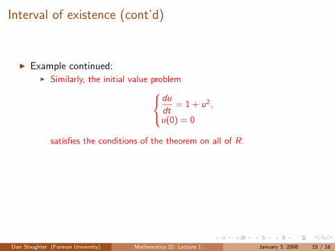
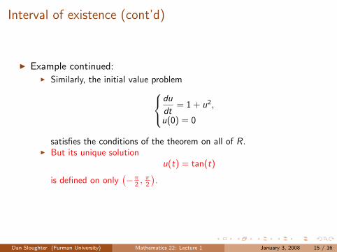
I Example continued:I Similarly, the initial value problem
du
dt= 1 + u2,
u(0) = 0
satisfies the conditions of the theorem on all of R.
I But its unique solutionu(t) = tan(t)
is defined on only(−π
2 ,π2
).
Dan Sloughter (Furman University) Mathematics 22: Lecture 1 January 3, 2008 15 / 16
Interval of existence (cont’d)
I Example continued:I Similarly, the initial value problem
du
dt= 1 + u2,
u(0) = 0
satisfies the conditions of the theorem on all of R.I But its unique solution
u(t) = tan(t)
is defined on only(−π
2 ,π2
).
Dan Sloughter (Furman University) Mathematics 22: Lecture 1 January 3, 2008 15 / 16
Example
I Recall: Both u ≡ 0 and u = 127 t3 are solutions ofdu
dt= u
23 ,
u(0) = 0.
I Reason: Although f (t, u) = u23 is continuous on all of R2,
fu(t, u) =2
3u13
is not continuous at any points of the form (t, 0) (that is, on theu-axis).
Dan Sloughter (Furman University) Mathematics 22: Lecture 1 January 3, 2008 16 / 16
![The De Continuo of Thomas Bradwardine - Furman …math.furman.edu/~dcs/sandiego.pdf · History or philsophy? I Etienne Gilson, in Being and Some Philosophers: I [The] author may well](https://img.pdfslide.net/doc/110x75/5ba7b09e09d3f20c5f8b7e2b/the-de-continuo-of-thomas-bradwardine-furman-math-dcssandiegopdf-history.jpg)