Mathematics 308—Fall 1996 Coordinate systems

Mathematics 308—Fall 1996

Coordinate systems

The aim of this chapter is to understand how PostScript deals with coordinate systems. The user does hisdrawing in user coordinates and PostScript renders them in page coordinates. It is important to understand thetransformation from one to the other. This part of PostScript is essentially mathematical, and rather elegant.

1. Summary of how to draw in PostScript

When you start a path, you put the command newpath into your program. Then you set a current point withthe moveto command and put in a number of commands adding pieces to the path you want to draw, such aslines or arcs of circles. Finally, you actually place the path on the current page with one of the three commandsstroke, fill or clip.

There are several different parameters involved in how the path is drawn. The most important are colour (for us,usually just a shade of grey), the line details, the clipping path and the transformation from the user coordinates topage coordinates.

We already know about most of these. A few extra remarks:

Colour. You always start off with colour black, which is 0 in a scale from 0 to 1. If you are a Canadian nationalistyou can put a line

/setgrey setgray def

and spell things the way you like. If you want to put the current shade on the stack you write

currentgray

so that if the current colour is either black or white the sequence

1 currentgray sub setgray

toggles it to the opposite shade.

Clipping. The clipping path sets a path outside which nothing is actually drawn. It gives you a kind of windowthrough which you will see your drawings. It is built like any other path, but replaces stroke or fill by clip.These are the only commands by which paths become part of your picture.

Line details. There are a number of other things you can specify—the width of lines, dash pattern, the way pathsare closed up, the way corners are rounded, etc.

Coordinates. In order to render pictures by programming commands, PostScript has to use a coordinate system ofsome kind. Of course at some point it has to keep track of the actual physical dimensions on the page. These arereferred to in page coordinates. But it would be a great nuisance if you yourself had to do all the computations inthese coordinates, as you would have had to in early printer control languages. Instead, PostScript has as part ofits environment a set of data which relate user coordinates to page coordinates. This way, you will rarely knowexactly what points on the page are involved in your drawing because PostScript will handle the calculations foryou internally.

When you start up, you will in fact be using page coordinates. One unit of drawing is equal to 1=72 of an inchon the page. This is for historical reasons—this unit is almost the same as a printer’s point, the unit used sinceearly in the history of printing to specify the size of letters on a printed page. Also, the origin of your coordinatesystem gets mapped onto the lower left of the page, and the x and y axes are perpendicular, going along the sidesof the page.

Coordinate systems 2

You can change these by using a number of commands, of varying complexity. The simplest are (1) scale, whichchanges the units in the x and y axes; (2) translate, which moves the origin; and (3) rotate, which rotatesthe axes. You can combine these in any order to get more complicated changes, and you can also change the wayin which your paths are rendered at a lower level.

Some mathematics is necessary in order to understand how this works. We must first look at how a number ofgeometrical features are specified in terms of coordinates.

2. Shears

A shear is a transformation of a 2D figure that has this effect:

It is a bit hard to describe in plain language. Its effect can perhaps be best realized by thinking of the rectangle asa side view of a deck of thick cards:

In other words it slides the components of a figure past each other, and it slides things further if they are higher.From this picture it should be at least intuitively clear that

� Shears preserve area.

Roughly speaking this is because sliding a very thin piece of a figure doesn’t change its shape. The actual proofthat a shear doesn’t change area is also very simple:

The idea is that we lop off a triangle from one end and shift it around to the other in order to make a parallelograminto a rectangle. The reason this works is because we can shift that triangle without distorting it. This reasoningalso shows that area = base � height. Of course we have to appeal to some more fundamental result to justifythis argument. A rigourous proof can be put together by discussing angles cut off by parallel lines. Ultimately itderives from Euclid’s parallel postulate, but I won’t discuss this further.

There are different directions of shearing possible. The one above is called a shear along the x axis. And thereare degrees of shear possible. We can specify a shear along the x axis completely with a single number whichtells us how much the unit square is transformed. Its base remains fixed, and the top moves parallel to the xaxis. The corner (0; 1) is moved to some point (a; 1). Where is the point (x; y) moved to? The y coordinateremains the same, and the horizontal distance moved (1) depends only the y coordinate; (2) is proportional to the


y coordinate. Therefore (x; y) is shifted by (ay; 0) and gets moved to (x+ ay; y). The effect can also be expressedby matrix multiplication: �

xy

�7!�1 a0 1

� �xy

�:

Therefore

� Shearing along the x axis is a linear transformation whose matrix is of the form

�1 a

0 1

�

3. Matrices and linear transformations

I recall that a linear transformation is a transformation of points in the plane which takes a point (x; y) to a point(x�; y�) whose coordinates are homogeneous linear functions of x and y. This means that

x� = ax+ by

y� = cx+ dy

for suitable coefficients a, b, c, d. Equivalently

�x�y�

�=

�a b

c d

� �x

y

�:

Let

e1 =

�1

0

�; e2 =

�0

1

�:

Another way of getting the matrix from the transformation is to keep in mind that

� If T is a linear transformation and A the matrix associated to it then the columns of A are the vectors whichT assigns to e1 and e2.

This is a simple calculation. Geometrically, this says that we can reconstruct the matrix of T if we know what Tdoes to the unit square 0 � x � 1, 0 � y � 1.

4. Length

The most important mathematical result we need is that which says that in a coordinate system where x and yare measured uniformly and in which the x and y axes are perpendicular to each other, the distance from theorigin to (x; y) is

px2 + y2. This is just Pythagoras’ Theorem. In order to reinforce how important it is, and

because readers may enjoy working their way through proofs of it, I shall include a discussion of why it is true.Of course, there are lots of different proofs of this result which been discovered in the more than 3000 years sincethe formula was discovered. We shall see two here and a few more in the exercises.

We begin with the statement:

� For a right triangle with short sides a and b and long side c we have c2 = a2 + b2.

Proof by dissection

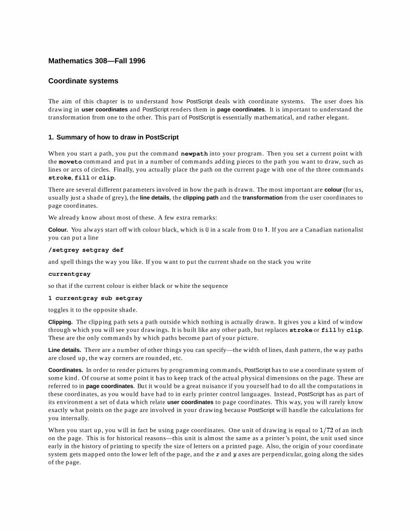
How satisfying a proof seems is to a large extent a matter of taste. The proof which I explain first is the one I preferto all others. It interprets the assertion geometrically in the most direct way possible. We can make Pythagoras’


assertion into a geometrical statement by constructing squares on the sides of the original triangle. The area ofthe large square is then to be the sum of the areas of the smaller squares.

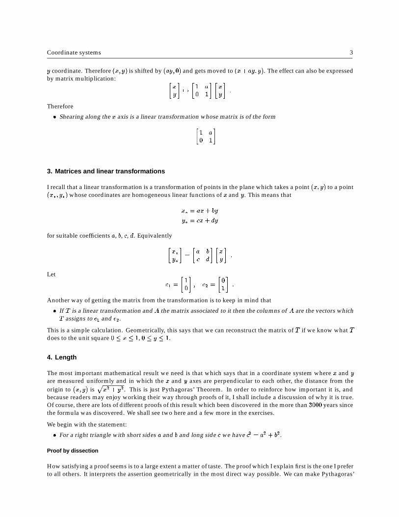
We can make this assertion more precise. Draw a straight line from the corner of the triangle where the rightangle occurs across the large square to its opposite side, where it meets that side at a right angle:

This line divides the large square into two rectangles, and a very explicit version of Pythagoras’ Theorem is thatthe area of each of these is equal to the area of one of the squares. In other words, Pythagoras’ Theorem is provenby dissecting the square of area c2 into two smaller pieces of area a2 and b2.

This claim is proven by applying a succession of transformations to a smaller square to turn it into its correspondingrectangle, while preserving its area. In practice we’ll go backwards. First we shear the rectangle one way:


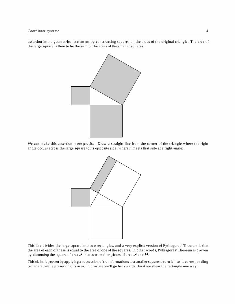
We know that area is preserved. To understand this step better, we can follow it from a different angle:

Then we shear the figure again, rotating the whole picture once more to let us visualize it better:


We have sheared the rectangle into a figure which is definitely a rectangle, and which in fact appears to be a copyof the small square. That it is one can be seen by using a rotation:

Of course the same sequence of transformations can be carried out for the other small square.

An algebraic proof

Consider the figure on the left below:


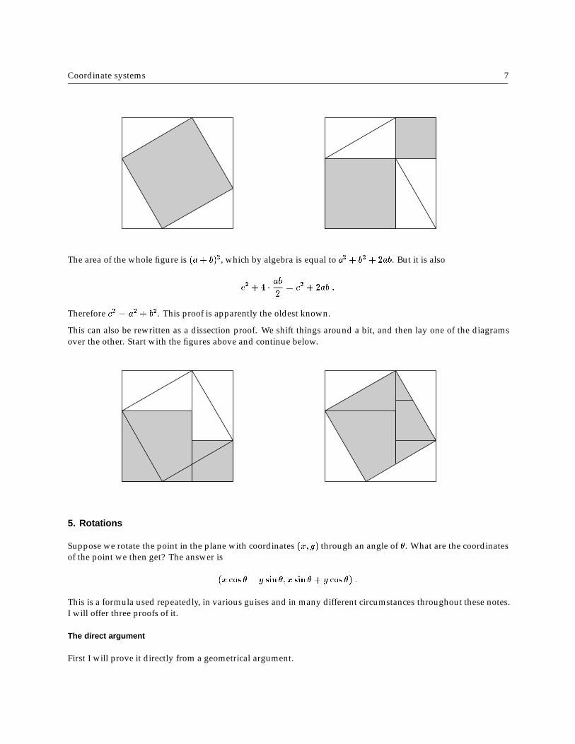
The area of the whole figure is (a+ b)2, which by algebra is equal to a2 + b2 + 2ab. But it is also

c2 + 4 � ab2

= c2 + 2ab :

Therefore c2 = a2 + b2. This proof is apparently the oldest known.

This can also be rewritten as a dissection proof. We shift things around a bit, and then lay one of the diagramsover the other. Start with the figures above and continue below.

5. Rotations

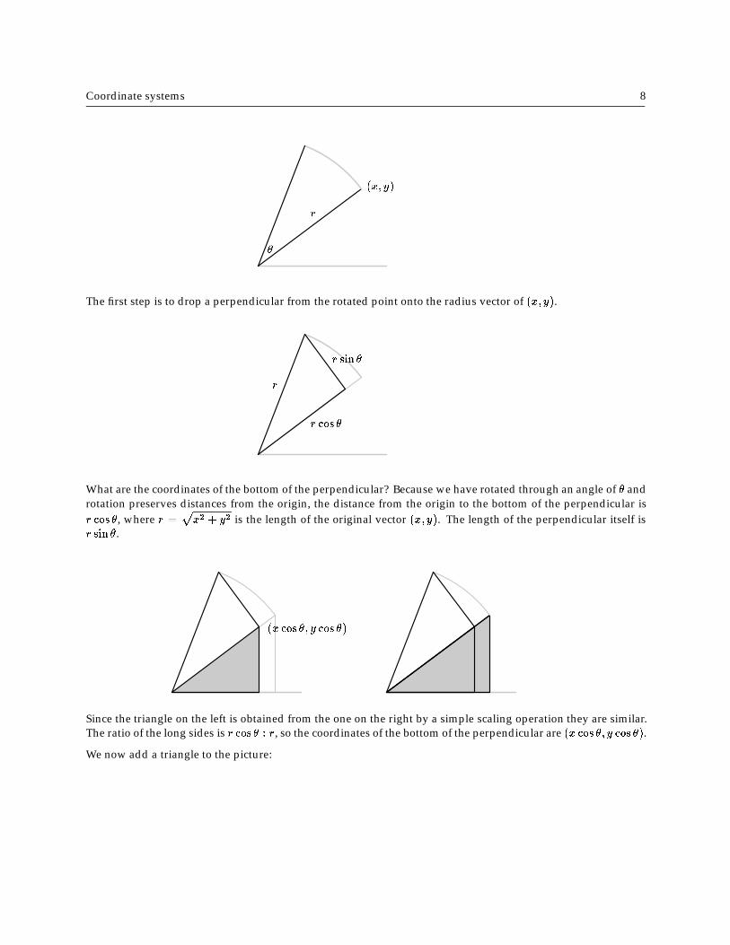
Suppose we rotate the point in the plane with coordinates (x; y) through an angle of �. What are the coordinatesof the point we then get? The answer is

(x cos � � y sin �; x sin � + y cos �) :

This is a formula used repeatedly, in various guises and in many different circumstances throughout these notes.I will offer three proofs of it.

The direct argument

First I will prove it directly from a geometrical argument.


(x; y)

r

�

The first step is to drop a perpendicular from the rotated point onto the radius vector of (x; y).

r cos �

r

r sin �

What are the coordinates of the bottom of the perpendicular? Because we have rotated through an angle of � androtation preserves distances from the origin, the distance from the origin to the bottom of the perpendicular isr cos �, where r =

px2 + y2 is the length of the original vector (x; y). The length of the perpendicular itself is

r sin �.

(x cos �; y cos �)

Since the triangle on the left is obtained from the one on the right by a simple scaling operation they are similar.The ratio of the long sides is r cos � : r, so the coordinates of the bottom of the perpendicular are (x cos �; y cos �).

We now add a triangle to the picture:


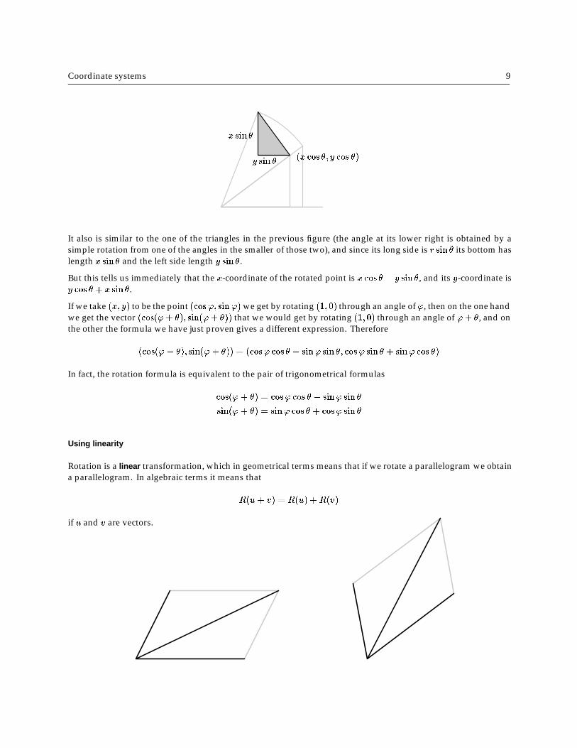
(x cos �; y cos �)

x sin �

y sin �

It also is similar to the one of the triangles in the previous figure (the angle at its lower right is obtained by asimple rotation from one of the angles in the smaller of those two), and since its long side is r sin � its bottom haslength x sin � and the left side length y sin �.

But this tells us immediately that the x-coordinate of the rotated point is x cos � � y sin �, and its y-coordinate isy cos � + x sin �.

If we take (x; y) to be the point (cos'; sin') we get by rotating (1; 0) through an angle of ', then on the one handwe get the vector (cos('+ �); sin('+ �)) that we would get by rotating (1; 0) through an angle of '+ �, and onthe other the formula we have just proven gives a different expression. Therefore

(cos('+ �); sin('+ �)) = (cos' cos � � sin' sin �; cos' sin � + sin' cos �)

In fact, the rotation formula is equivalent to the pair of trigonometrical formulas

cos('+ �) = cos' cos � � sin' sin �

sin('+ �) = sin' cos � + cos' sin �

Using linearity

Rotation is a linear transformation, which in geometrical terms means that if we rotate a parallelogram we obtaina parallelogram. In algebraic terms it means that

R(u+ v) = R(u) +R(v)

if u and v are vectors.


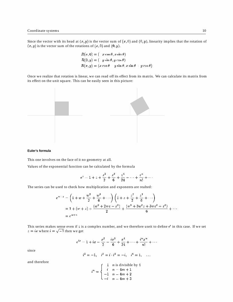
Since the vector with its head at (x; y) is the vector sum of (x; 0) and (0; y), linearity implies that the rotation of(x; y) is the vector sum of the rotations of (x; 0) and (0; y).

R(x; 0) = ( x cos �; x sin �)

R(0; y) = (�y sin �; y cos �)R(x; y) = (x cos � � y sin �; x sin � + y cos �)

Once we realize that rotation is linear, we can read off its effect from its matrix. We can calculate its matrix fromits effect on the unit square. This can be easily seen in this picture:

Euler’s formula

This one involves on the face of it no geometry at all.

Values of the exponential function can be calculated by the formula

ez = 1 + z +z2

2+z3

6+

z4

24+ � � � + zn

n!+ � � �

The series can be used to check how multiplication and exponents are realted:

ew+z =

�1 +w +

w2

2+w3

6+ � � �

��1 + z +

z2

2+z3

6+ � � �

�

= 1 + (w + z) +(w2 + 2wz + z2)

2+

(w3 + 3w2z + 3wz2 + z3)

6+ � � �

= ew+z

This series makes sense even if z is a complex number, and we therefore useit to define ez in this case. If we setz = ix where i =

p�1 then we get

eix = 1 + ix� x2

2� ix3

6+x4

24+ � � � + inxn

n!+ � � �

sincei2 = �1; i3 = i � i2 = �i; i4 = 1; : : :

and therefore

in =

8><>:

1 n is divisible by 4

i n = 4m+ 1

�1 n = 4m+ 2

�i n = 4m+ 3


The series for eix can be rewritten as

eix = 1 + ix� x2

2� ix3

6+x4

24+ � � � + inxn

n!+ � � �

=

�1� x2

2+x4

24� � � �

�+ i

�x� x3

6+

x5

120� � � �

�

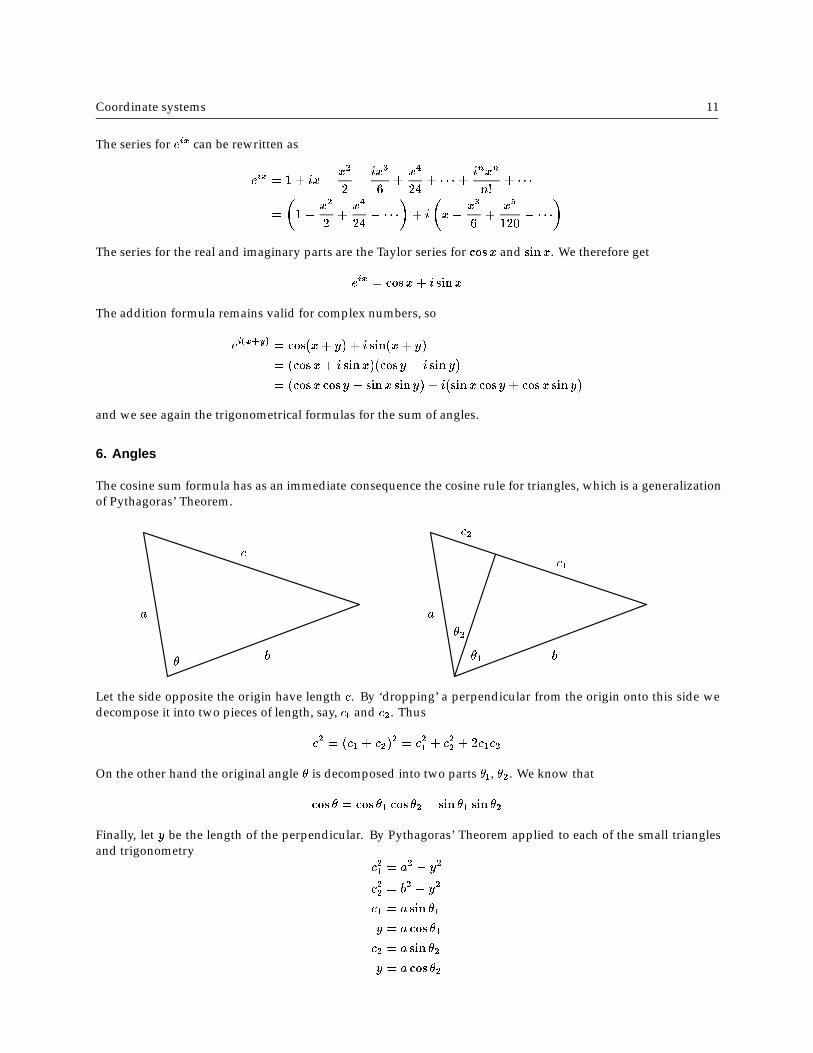
The series for the real and imaginary parts are the Taylor series for cosx and sinx. We therefore get

eix = cosx+ i sinx

The addition formula remains valid for complex numbers, so

ei(x+y) = cos(x+ y) + i sin(x+ y)

= (cosx+ i sinx)(cosy + i sin y)

= (cosx cosy � sinx siny) + i(sinx cosy + cosx siny)

and we see again the trigonometrical formulas for the sum of angles.

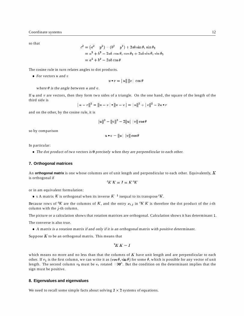
6. Angles

The cosine sum formula has as an immediate consequence the cosine rule for triangles, which is a generalizationof Pythagoras’ Theorem.

�

a

b

c

�2

�1

a

b

c1

c2

Let the side opposite the origin have length c. By ‘dropping’ a perpendicular from the origin onto this side wedecompose it into two pieces of length, say, c1 and c2. Thus

c2 = (c1 + c2)2 = c21 + c22 + 2c1c2

On the other hand the original angle � is decomposed into two parts �1, �2. We know that

cos � = cos �1 cos �2 � sin �1 sin �2

Finally, let y be the length of the perpendicular. By Pythagoras’ Theorem applied to each of the small trianglesand trigonometry

c21 = a2 � y2

c22 = b2 � y2

c1 = a sin �1

y = a cos �1

c2 = a sin �2

y = a cos �2


so thatc2 = (a2 � y2) + (b2 � y2) + 2ab sin �1 sin �2

= a2 + b2 � 2ab cos �1 cos �2 + 2ab sin �1 sin �2

= a2 + b2 � 2ab cos �

The cosine rule in turn relates angles to dot products.

� For vectors u and vu � v = kuk kvk cos �

where � is the angle between u and v.

If u and v are vectors, then they form two sides of a triangle. On the one hand, the square of the length of thethird side is

ku� vk2 = ku� vk � ku� vk = kuk2 + kvk2 � 2u � v

and on the other, by the cosine rule, it is

kuk2 + kvk2 � 2kuk kvk cos�

so by comparisonu � v = kuk kvk cos�

In particular:

� The dot product of two vectors is 0 precisely when they are perpendicular to each other.

7. Orthogonal matrices

An orthogonal matrix is one whose columns are of unit length and perpendicular to each other. Equivalently, Kis orthogonal if

tKK = I = K tK

or in am equivalent formulation:

� s A matrix K is orthogonal when its inverse K�1 isequal to its transpose tK .

Because rows of tK are the columns of K , and the entry xi;j in tKK is therefore the dot product of the i-thcolumn with the j-th column.

The picture or a calculation shows that rotation matrices are orthogonal. Calculation shows it has determinant 1.

The converse is also true.

� A matrix is a rotation matrix if and only if it is an orthogonal matrix with positive determinant.

Suppose K to be an orthogonal matrix. This means that

tKK = I

which means no more and no less than that the columns of K have unit length and are perpendicular to eachother. If v1 is the first column, we can write it as (cos �; sin �) for some �, which is possible for any vector of unitlength. The second column v2 must be v1 rotated �90�. But the condition on the determinant implies that thesign must be positive.

8. Eigenvalues and eigenvalues

We need to recall some simple facts about solving 2� 2 systems of equations.


If A is a 2� 2 matrix its transpose adjoint tA� is defined by the prescription

A =

�a1;1 a1;2a2;1 a2;2

�; tA� =

�a2;2 �a1;2

�a2;1 a1;1

�:

A simple calculation shows that

A tA� =

�det(A) 0

0 det(A)

�

so that if det(A) = a1;1a2;2 � a1;2a2;1 6= 0 then

A�1 =1

det(A)

tA� =

�a2;2=det �a1;2=det

�a2;1=det a2;2=det

�:

In this case if we are given an equation Au = 0 we can multiply on both sides by A�1 to get u = A�10 = 0.

If det(A) = 0 then both of the columns of tA� are vectors u such that

Au = 0

If A is not itself the 0 matrix at least one of these columns is not the 0 vector, and otherwise A annihilaites allcolumn vectors.

� If A is a 2� 2 matrix then exactly one of these possibilities occurs:(1) the matrix A is invertible, det(A) 6= 0, and the only vector annihilated by A is the 0 vector itself;(2) the matrix A is singular, det(A) = 0, and there exists a non-zero vector u such that Au = 0.

An eigenvector of a linear transformation T is a vector v 6= 0 taken into a multiple of itself by T :

Tv = �v

for some scalar �. The scalar is called the associated eigenvalue. IfM is the matrix of T then to find an eigenvectorv we must solve

M

�x

y

�= �

�x

y

�; v =

�x

y

�:

This can be rewritten as(M � �I)v = 0

where I is the identity matrix

I =

�1 0

0 1

�:

Since by definition an eigenvector is not 0, we must therefore have

det(M � �I) = 0 :

If

M =

�a b

c d

�

then

M � �I =

�a� � b

c d� �

�

and � must be a root of the characteristic polynomial

�2 � (a+ d)�+ (ad� bc) = 0 :


The system of equations to determine the coordinates of an eigenvector is then

(a� �)x+ by = 0

cx+ (d� �)y = 0 :

Since the coefficient matrix is singular, one of these equations is a multiple of the other, and we need to consideronly one of them. Most of the time we can set

x = b; y = (�� a) :

Often we want eigenvectors of length 1, in which case we divide x and y by r =px2 + y2.

Example. Let

M =

�1 1

1 2

�:

Its characteristic polynomial is�2 � 3�+ 1 = 0

so its eigenvalues are 3=2�p5=2 = �1, �2; numerically �1 = 2:618034, �2 = 0:381966. To find the eigenvectorsfor � we solve �

1 1

1 2

� �xy

�= �

�xy

�

and get the eigenvector equation(1� �)x+ y = 0 :

Explicitly, the eigenvector for �1 is �0:5257310:850651

�

If M is a matrix and v1, v2 are eigenvectors for M with eigenvalues �1 , �2 then

Mv1 = �1v1; Mv2 = �2v2 :

If we make up a matrix V whose columns are the vi then

MV = M [ v1 v2 ] = [Mv1 Mv2 ] = [�1v1 �2v2 ] = [ v1 v2 ]

��1 0

0 �2

�= V D

andM = V DV �1 :

In this course, with perhaps a few exceptions, the matrix M will be symmetric. If

M =

�a b

b c

�

then its eigenvalues area + c

2�p

(a� c)2 + 4b2

2

and are both real. To avoid problems with rounding we calculate one root � by this formula, the one where thesign of the square root is the same as the sign of a+ c, and calculate the other as det =�.

9. Scaling


A scale change along the x and y axes is a transformation which multiplies all x coordinates by one factor and ally coordinates by another. Since it takes (x; y) to (ax; by). it has a matrix of the form

�a 0

0 b

�:

There are other scale changes. The most general possible ones are those which change scale along some pair oforthogonal axes.

How can we find the matrix of a general scale change T ? Let v1 and v2 be orthogonal vectors of unit length andpositive orientation along the axes of the scale change. Then

R = [ v1 v2 ] =

�v1;x v2;xv1;y v2;y

�

is a rotation matrix, say for angle �. Suppose T scales along the line through v1 by a and along that through v2by b. To find what the matrix of T is we must find what it does to the vectors e1 and e2? Then by definition ofcoordinates we have

v1 = (cos �) e1 + (sin �) e2

v2 = �(sin�) e1 + (cos �) e2

ore1 = (cos �) v1 � (sin �) v2

e2 = (sin�) v1 + (cos �) v2

ThereforeTe1 = a(cos �) v1 � b(sin�) v2

Te2 = a(sin �) v1 + b(cos�) v2

We now substitute for v1 and v2 in terms of e1 and e2. The final result is very simple:

� If T is a scale change whose axes are the columns of the rotation matrix R with scale factors a and b then thematrix of T is

MT = RAR�1

where

A =

�a 0

0 b

�:

The matrix MT is symmetric sinceMT = RAR�1

= RA tRtMT = R tA tR

= RA tR

= MT :

Conversely, ifM is a symmetric matrix it has real eigenvalues and we can find orthogonal eigenvectors. The lineartransformation associated to M will be a scale change along the axes determined by its eigenvectors. Thereforethe matrices of scale changing transformations coincide exactly with the symmetric matrices.

Some of them will scale by positive factors. The ones we shall meet will generally arise in the same way.

� If M is any matrix then the matrix tMM is symmetric and has non-negative eigenvalues.


The proof hinges on a fundamental equation involving dot products and matrix transposes. If u and v are columnvectors of dimension 2 then their dot product can be expressed also as a matrix product:

u � v = u1v1 + u2v2 = [ u1 u2 ]

�v1v2

�= tu v :

If u is an eigenvector of tMM with eigenvalue c then tMMu = cu. But then

tMMu �u = cu �u = c kuk2

on the one hand andMu �Mu = kMuk2

on the other. But ifkMuk2 = c kuk2

then since u cannot be 0, c must be non-negative.

10. Factoring linear transformations

The key result in this section is this:

� Any linear transformation can be written as a composition R1SR�12 where R1 and R2 are rotations and S is

a scale change along the x and y axes.

I shall prove this by finding the matrices of all these transformations explicitly. It is a somewhat messy computa-tion.

It depends on being able to find eigenvalues. There is one case which is straightforward, and that is where M issymmetric. In that case

M = RSR�1

where S is a diagonal matrix with entries are the eigenvalues of M and the columns of R are its eigenvectors.The matrix R can be chosen to be a rotation matrix, in which case R�1 is also one.

Let M be an arbitrary invertible matrix. If we could write

M = R1SR�12

where the Ri are rotations, then tS = S so

tMM = R2StR1R1SR

�12 :

Recall that t(AB) = tBtA. Since tR1R1 = I , we also have

tMM = R2S2R�1

2 :

This means that the columns of R2 are the eigenvectors of tMM and that the entries of S2 are the squares of itseigenvalues.

This suggests how to start with M and find the Ri and S. Let M be an arbitrary matrix. If we write

tMM =

�a cb d

� �a bc d

�=

�a2 + b2 ac+ bdac+ bd c2 + d2

�

we see that the matrix tMM is symmetric. We know already that it has non-negative eigenvalues. Therefore wecan write

tMM = R2DR�12


where the columns of R2 are the eigenvectors of tMM . We know that the eigenvalues of M , the diagonal entriesof D, are non-negative, so we can write D = S2 with S diagonal. There is a choice of sign—if detM < 0, chooseone sign along the diagonal of A negative. This ensures detS = detM . We now want

M = R1SR�12

so we setR1 = MR2S

�1 :

I claim that R1 is a rotation matrix.

We apply the earlier result. The determinant of R2 is positive because determinants multiply and

detR2 = detS detR�11 detM = detS detM

and because of the choice of signs of S. Furthermore

R�11 R1 = tR1R1 = S�1R�1

2tMMR2 SS�1R�1

2 R2 S2R�12 R2 S = I :

Note that all these steps can be carried out explicitly, if painfully.

Summary. Let

M =

�a b

c d

�

(1) CalculatetMM =

�a2 + b2 ac+ bd

ac+ bd c2 + d2

�=

�A B

B C

�; D = det(tMM) = AC �B2 :

(2) Let � be one of the eigenvalues

� =A+ C

2+

p(A+C)2 � 4D

2:

(3) Let

x = B; y = � �A; r =px2 + y2; u =

�x=ry=r

�

so that u is a normalized eigenvector of tMM , and let

u =

��y=rx=r

�

be v rotated by 90�.

(4) Let

R2 = [u v ] ; S =

�p� 0

0 det(M)=p�

�:

Then calculateR1 = MR2S

�1 :

We have M = R1SR�12 .

Example. Suppose we are given the matrix

M =

�1 1

0 1

�:


ThentMM =

�1 1

1 2

�:

Its characteristic polynomial is�2 � 3�+ 1 = 0

so its eigenvalues are 3=2�p5=2 = �1, �2; numerically �1 = 2:618034, �2 = 0:381966. The eigenvector for � is

�0:525731

0:850651

�

which makes

R2 =

�0:525731 �0:850651

0:850651 0:525731

�

and

S =

�1:618034 0:0000000:000000 0:618034

�

Finally

R1 = MR2S�1 =

�0:850651 �0:5257310:525731 0:850651

�

A consequence of this factorization:

� A linear transformation changes areas by a factor equal to its determinant. It preserves orientations if andonly if its determinant is positive.

This is because any linear transformation can be factored as above, and determinants and volume change factorsmultiply under composition.

11. Affine transformations

Suppose given two planes, each with rectangular coordinates. If A is a 2 � 2 matrix and (�x; �y) a vector in thesecond plane, then the map taking �

xy

�7! A

�xy

�+

��x�y

�

is called an affine transformation. In short, an affine transformation is a linear transformation followed by a vectortranslation.

Explicitly, if

A =

�a bc d

�

then this map takes �xy

�7!�uv

�=

�ax+ bycx+ dy

�+

��x�y

�=

�ax+ by + �xcx+ dy + �y

�:

� If A is an invertible matrix, then this transformation is invertible.

This is because we can solveu = ax+ by + �x

v = cx+ dy + �y

orax+ by = u� �x

cx+ dy = v � �y


for (x; y) if we are given (u; v). In terms of matrices if

�u

v

�= A

�x

y

�+

��x�y

�

then �xy

�= A�1

�uv

�� A�1

��x�y

�

so that the inverse is also an affine transformation.

� An affine transformation takes lines to lines.

Let ` be a parametrized line of the form

t 7!�x0y0

�+ t

�p

q

�=

�x0 + tp

y0 + tq

�

that is to say going through (x0; y0) in the direction (p; q). Then T` goes through

A

�x0y0

� ��x�y

�

in the direction

A

�pq

�:

Affine transformations can be characterized in completely geometric terms as maps from one plane to anotherwhich take lines to lines. But this is a subtle fact. I explain it an appendix to this section.

12. The transformation matrix in PostScript

Implicit in PostScript drawing are two coordinates, user coordinates and page coordinates. When the programmerdraws a line from one point to the other he specifies their coordinates in the user system, and then PostScriptrenders them into positions on the page. The transformation it applies to go from user coordinates to pagecoordinates has, in general, no other property than that it takes straight lines to striaght lines. It can be anarbitrary affine transformation.

It is represented in PostScript by an array of six elements

[a b c d tx ty]

representing the matrix A and translation vector � . It is called the Current Transform Matrix or CTM for short. Theconventions of interpreting these coefficients are a little different from what we are used to, however, because

� In PostScript all vectors are row vectors and matrices are applied on the right.

This is a common problem in computer graphics, where the community seems about evenly divied between rowand column interpretation of vectors. Thus the effect of the CTM on coordinates (x; y) is to change them to

[ x y ]

�a b

c d

�+ [ �x �y ]

This is something to be careful about, but shouldn’t cause serios difficulties. In PostScript it is justifiable becauseafter all it does calculations backwards anyway.

The CTM is modified by the commands rotate, translate, and scale as well as others.

(�) The effect of the sequence


sx sy translate

is to change the CTM to [a b c d tx+sx ty+sy].

(�) The effect of

sx sy scale

is to change the CTM by multiplying its linear component A (the 2� 2 matrix) by a diagonal matrix:

A 7!�sx 0

0 sy

�A

(�) The effect of rotate is

A 7!�

cos � sin �

� sin � cos �

�A

To understand this, keep in mind that the matrix of a rotation by � is

�cos � sin �

� sin � cos �

�

If this is different from what you are used to it is because here matrices act on the right.

Any affine transformation can be represented as a linear transformation in three dimensions. We do this byidentifying the (x; y) plane with the plane z = 1 in three dimensions. The matrix

24 a b 0

c d 0

�x �y 1

35

takes this plane to itself, and has the same effect onx and y coordinates as the corresponding affine transformationdoes. To see this, calculate

[ x y 1 ]

24 a b 0

c d 0

�x �y 1

35

This representation has the virtue that the composition of transformations corresponds to the multiplication ofmatrices. There is a PostScript command which does exactly that for you.

(�) The sequence

[a b c d tx ty] concat

replaces the CTM by the matrix product 24 a b 0

c d 0

�x �y 1

35CTM

if we think of the CTM as a 3� 3 matrix.

It is also possible to set the CTM directly instead of just modifying it, but this is such a terrible idea that I won’ttell you how to do it.

In general, it is not a good idea to use concat as opposed to applying a succession of translations, scale changes,and rotations. There is no loss of flexibility. It is an easy consequence of the factorization of linear transformationsthat one can also factor affine transformations:

� Any affine transformation can be represented as a composition of rotations, scale changes, and translations.


Still, it is at least conceivable that you might want to apply a shear to your picture, in which case concat is whatyou should use.

13. Ellipses

An ellipse is what you get when you scale a unit circle in perpendicular directions, along axes through its centre.Accordng to this definition, a circle is to be considered as a special kind of ellipse.

The data specifying an ellipse comprise the original circle, or equivalently the centre of the circle, together withthe scaling factors and axes. Unless the ellipse is a circle, these data are uniquely determined by the ellipse. Ifwe start with the unit circle and scale it, rotate it, and then translate it, we can obtain any given ellipse. Since anyaffine transformation can be obtained a composition of such operations, its effect on any circle will be to producean ellipse. This is not quite obvious—for example, if you shear the unit circle along the x-axis it is true that youwill get an ellipse, but the axes of this ellipse are not at all easy to calculate, and in fact it is not at all clear a priorithat the figure you get has any axis of symmetry much less two orthogonal ones.

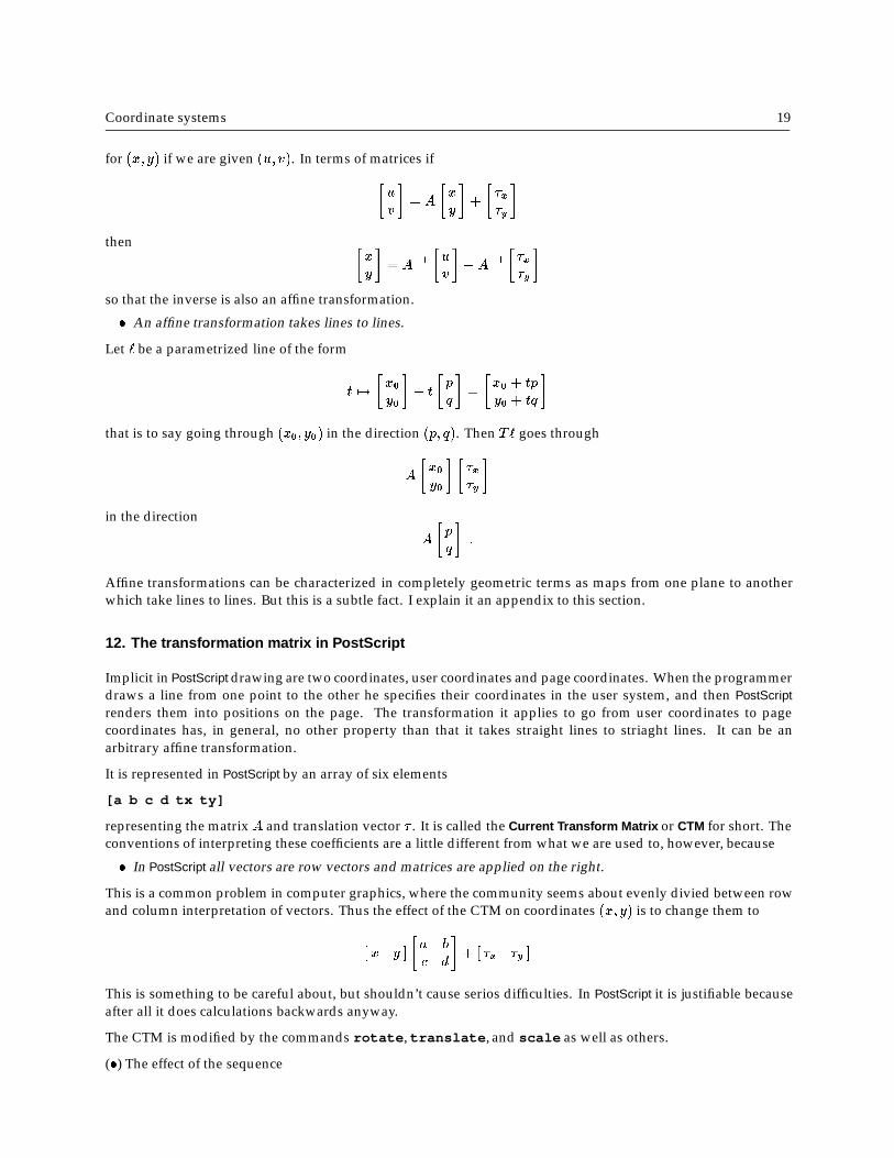
For example since

�1 1

0 1

�=

�0:850651 �0:525731

0:525731 0:850651

� �1:618034 0

0 0:618034

� �0:525731 0:850651

�0:850651 0:525731

�

it takes the unit circle to an ellipse with major half-diameter 1:618034, minor half-diameter 0:618034, and whosemajor axis goes through (0:850651; 0:525731) and has an angle of about 32� with respect to the x-axis.

Incidentally, you draw circles in PostScript with the command arc. The sequence

1 0 moveto0 0 10 0 360 arcstroke

draws a circle (an arc from 0� to 360�) of radius 10 with centre (0; 0). The command arc has what at first sightis a peculiar property—it adds the arc to any current path, so that in order to avoid an extra straight line in yourpicture you may have to move to the initial point of the arc. We shall see later that this apparent peculiarity isactually a natural way to implement curve drawing.

Exercise 13.1. The ellipse above was made with concat and then drawing a circle. Write a few lines in PostScriptwhich will draw the complete ellipse and its axes.

Exercise 13.2. In the proof of the angle-sum formula using Euler’s formula there wasn’t any apparent geometry.This is impossible, and there must be some hidden somewhere. Where exactly?


Exercise 13.3. If we are given two sets of three points each in the plane, and each set of three is non-collinear, thenthere exists a unique affine transformation taking one to the other. Write down in your own words a sequence ofcalculations that will find it.

Exercise 13.4. Find the unique affine transformation explicitly when the first three are (1; 1), (�1; 2), (1; 3) andthe second three are (1;�1), (2; 3), (2;�2). Express it in PostScript form (as an array of 6 elements, acting on theright). Also write down the 3� 3 matrix corresponding to it.

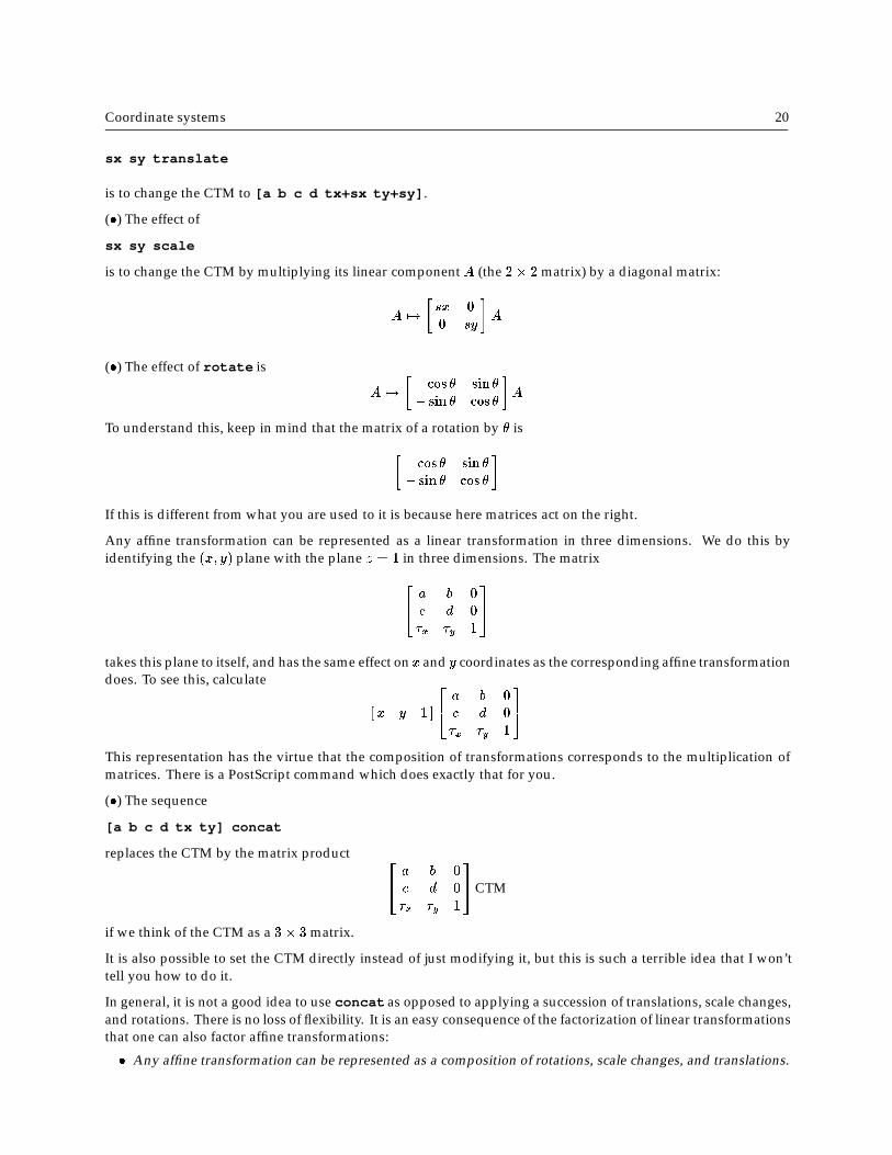
Exercise 13.5. The following three pictures accompany two proofs of the Pythagoras theorem. (The first is fromthe proof of Proposition 47 in Euclid.)

Write proofs to match the pictures. Your proofs should not label points and lines unless absolutely necessary.Instead, I want you to use colouring schemes and lots of drawings to explain what is going on.

There are three diagonal lines which seem to intersect towards the middle of the triangle on the left. Do they infact intersect, or is it only an artifact of the drawing? Reasons?

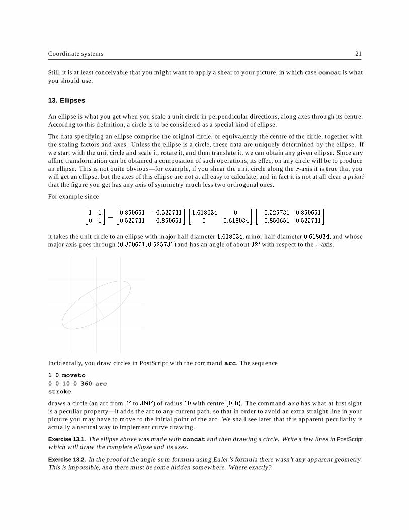
Exercise 13.6. Here is yet another picture for you to translate into a proof of Pythagoras’ Theorem. The first trickis to find the triangle!

Documents

Mathematics 308—Fall 1996 Coordinate systems