Embed Size (px)
Citation preview

Mathematics and Statistics for International Development Engineering
Yukihiko YamasitaDept. of International Development Engineering
Tokyo Institute of Technology
Contents1. Linear algebra
2. Statistical estimation
3. Optimization
1

1 Introduction1.1 PurposeTo learn basic mathematics and Statistics for international development.
1.2 Linear algebra• Eigenvalue problem
– Physical analysis– Statistical Optimization (Dimensional reduction)
• Singular value decomposition (SVD)– Approximation of a matrix– Regularization (rank reduction)
• Generalized inverses of matrix– Inverse filter– Limit of regularization
• Octave (GPL Software for linear algebra)
2

1.3 Statistical estimationEstimate the origin from results.
• Random variable•Mean and variance•Well-known Probabilistic distributions including• Characterization of normal distribution• Coordinate transform• Test (Kentei)• Estimator (Suiteiryou), estimate (Suiteichi)• Unbiased estimator• Cramer-Rao lower bound for unbiased estimators• Statistical learning theory
3

1.4 Optimization• Optimization is very important. It is used for calculating
– Statistical estimation,– Economical planing,– Environmental assessment.
• Gradient method– Maximum gradient method– Conjugate gradient method
• Newton’s method (quasi-Newton’s method)– Second order derivatives are considered.
• Conditional optimization• Support vector machine for pattern recognition
4

1.5 global maximum vs. local maximum
•We can only see our neighborhood.– Assume that we optimize
f (x1, x2, . . . , xN),– search 10 points for each xi.⇒ calculation at 10N points.⇒ It is impossible when N is large.
• No method to solve this problem in general.Heuristic methods :– Inertia term :α · (new change) + (1 − α) · (previous change)
– Homotopy method :a simple function→ a complex function
– Simulated annealing.– GA (generic algorithm).
5

1.6 Schedule
10/8 IntroductionProjection matrix
10/15 Eigenvalue problemSingular value problem
10/22 Generalized inverse10/29 Octave
(Program for linear algebra)11/5 Probability I11/6 Probability II11/19 Normal distribution
11/26 Test and Estimation I12/3 Test and estimation II12/10 Cramer-Rao lower bound12/17 Statistical learning theory12/24 Maximum gradient method
Conjugate gradient method1/7 quasi-Newton’s method1/14 Conditional optimization1/25 Support Vector Machine
6

2 Eigenvalue problem2.1 Range and null space of a matrixDefinition• Rn : n-dimensional real vector space• S is a subspace if and only if for any vectors x and y in S and any scalarsα and β,
αx + βyis in S .• R(A) ≡ Ax | x ∈ Rm : the range of an (n,m)-matrix A• N(A) ≡ x ∈ Rm | Ax = 0 : the null space of an (n,m)-matrix A• R(A) and N(A) are subspaces.
(Proof.) If x, y ∈ R(A), there exist f and g such that x = A f and y = Ag.Then, αx + βy = αA f + βAg = A(α f + βg) yields αx + βy ∈ R(A).If x, y ∈ N(A), we have Ax = 0 and Ay = 0. Then, A(αx + βy) = 0 sothat αx + βy ∈ N(A).
Problem 1. Prove the underlined equation A(αx + βy) = 0.7

2.2 Projection Matrix (Projector)Definition 1. A matrix P is a projection matrixif and only if P2 = P.
For a projection matrix P, we have
Px = P2x = P3x = P4x = · · ·Lemma 1. For a projection matrix P, We have
R(P) = N(I − P), (1)N(P) = R(I − P), (2)
R(P) ∩ N(P) = 0, (3)R(P) + N(P) = Rn. (4)
Remarks:• The sum of subspaces R(P) and N(P) isRn.• The intersection of R(P) and N(P) is only
0
• P is the projectionmatrix onto R(P)along N(P).
8
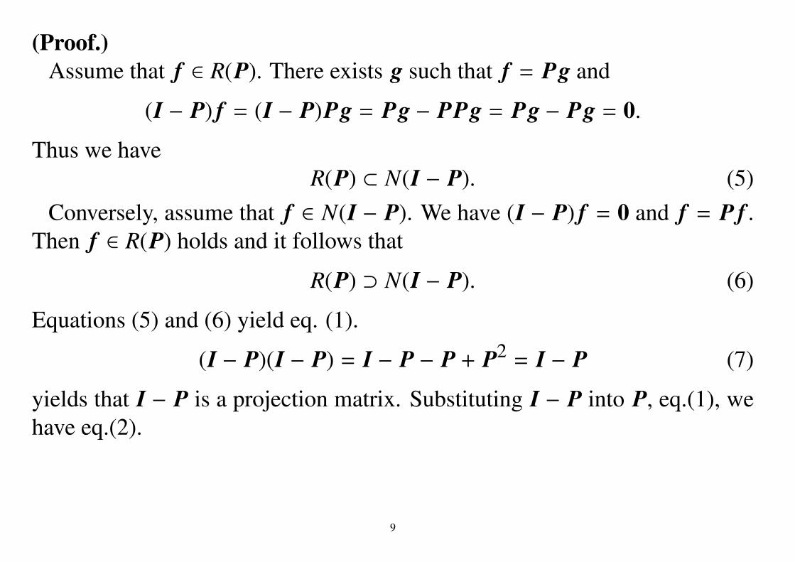
(Proof.)Assume that f ∈ R(P). There exists g such that f = Pg and
(I − P) f = (I − P)Pg = Pg − PPg = Pg − Pg = 0.
Thus we haveR(P) ⊂ N(I − P). (5)
Conversely, assume that f ∈ N(I − P). We have (I − P) f = 0 and f = P f .Then f ∈ R(P) holds and it follows that
R(P) ⊃ N(I − P). (6)
Equations (5) and (6) yield eq. (1).
(I − P)(I − P) = I − P − P + P2 = I − P (7)
yields that I − P is a projection matrix. Substituting I − P into P, eq.(1), wehave eq.(2).
9

When f ∈ R(P), there exists g such that f = Pg. Then, we have
f = Pg = PPg = P f
Assume that f ∈ R(P) ∩ N(P) = R(P) ∩ R(I − P). Then, f = P f andf = (I−P) f hold so that we have f = P f = P(I−P) f = (P−PP) f = O f = 0and eq.(3). In general, we have R(A + B) ⊂ R(A) + R(B) for any matrices Aand B, then eq.(4) holds. QED (quod erat demonstrandum).
Problem 2. Proof the underlined formula R(A + B) ⊂ R(A) + R(B)
10

2.2.1 Orthogonal projection matrix
Definition 2. For vectors x and y and sub-spaces S 1 and S 2,
• x ⊥ y : ⟨x, y⟩ = 0,• x ⊥ S 1 : ⟨x, y⟩ = 0 for any y ∈ S 1,• S 1 ⊥ S 2 : ⟨x, y⟩ = 0 for any x ∈ S 1 and
any y ∈ S 2.• S⊥ = x ∈ Rn | x ⊥ S
Lemma 2. Let S 1 and S 2 be subspaces. IfS 1 ⊂ S 2, then
S⊥1 ⊃ S⊥2 .
(Proof.)Since S 1 ⊂ S 2, y ∈ S⊥2 yields that y ∈ S⊥1 .QED.
Lemma 3. For a sub-space S we have
S⊥⊥ = S .
For the proof, the ex-istence of the orthogo-nal projection has to beproved (difficult).
11

Lemma 4. Let S 1 and S 2 be subspaces. We have
(S 1 ∩ S 2)⊥ = S⊥1 + S⊥2(=
x + y | x ∈ S⊥1 , y ∈ S⊥2
)(Proof.)
(S 1 ∩ S 2)⊥ ⊃ S⊥1 and (S 1 ∩ S 2)⊥ ⊃ S⊥2 yield (S 1 ∩ S 2)⊥ ⊃ S⊥1 + S⊥2 .(S⊥1 + S⊥2 )⊥ ⊂ (S⊥1 )⊥ = S 1 and (S⊥1 + S⊥2 )⊥ ⊂ (S⊥2 )⊥ = S 2 yield
(S⊥1 + S⊥2 )⊥ ⊂ S 1 ∩ S 2 and S⊥1 + S⊥2 ⊃ (S 1 ∩ S 2)⊥. QED.
Lemma 5. Let AT be the transposition of A. We have
R(AT ) = N(A)⊥ (8)N(AT ) = R(A)⊥ (9)
(Proof.)For all x ∈ R(A)⊥, we have ⟨x, Ay⟩ = 0 for all y ∈ Rm.⇒ ⟨AT x, y⟩ = 0⇒ AT x = 0⇒ x ∈ N(AT )⇒ R(A)⊥ ⊂ N(AT ).
Conversely, for all x ∈ N(AT ) and all y ∈ Rm,0 = ⟨AT x, y⟩ = ⟨x, Ay⟩ ⇒ x ∈ R(A)⊥⇒ N(AT ) ⊂ R(A)⊥.
Then, eq.(9) is proved. The rest of this lemma is clear. QED.12

Problem 3. Prove the underlined sentence.Hint: Use (AT )T = A and S = T yields S⊥ = T⊥.Lemma 6. PT is the projection matrix onto N(P)⊥ along R(P)⊥.(Proof.)
PT PT = (P2)T = PT
and Lemma 5 yield the lemma. QED.Definition 3. A matrix P is an orthogonal projection matrix if and only if
PT P = P. (10)
Remark: Since P = PT yields N(P) = N(PT ) = R(P)⊥, it can be called theorthogonal projection matrix.Remark: Equation (10) is equivalent to the following system of equations.
P2 = P (11)PT = P (12)
(Proof.)When PT P = P, we have PT = (PT P)T = PT P = P. QED.
13

Lemma 7. For any x ∈ Rn, Px provides the nearest element in R(P).
(Proof.)For any element y ∈ R(P), Py = y and PT (I − P) = PP − P = O yield
∥x − y∥2 = ∥x − Px + Px − y∥2 = ∥(I − P)x + P(x − y)∥2= ⟨(I − P)x + P(x − y), (I − P)x + P(x − y)⟩= ∥(I − P)x∥2 + 2⟨(I − P)x, P(x − y)⟩ + ∥P(x − y)∥2= ∥x − Px∥2 + 2⟨PT (I − P)x, x − y⟩ + ∥Px − Py∥2= ∥x − Px∥2 + ∥Px − y∥2≥ ∥x − Px∥2.
The inequality∥x − y∥2 ≥ ∥x − Px∥2
implies that Px is the nearest to x in R(P). QED.
14

2.3 EigenequationA : a symmetric real (n, n)-matrixEigenequation
Ax = λx (13)λ : eigenvaluex : eigenvector (x , 0)
There exist n solutions (including degeneration):eigenvalue: λ1 ≥ λ2 ≥ · · · ≥ λneigenvector: u1,u2, . . . , un
Aui = λiui
We can choose uini=1 as an orthonormal basis (ONB) :
⟨ui,u j⟩ = δi, j =
1 (i = j)0 (i , j) (14)
15

(Proof.)From eq.(13), we have
(A − λI)x = 0, (15)where I is a unit matrix. Since x , 0, Ax−λI must not be regular. Therefore,
det(A − λI) = 0. (16)This is a polynomial of degree n with respect to λ. There exist n solutions inC (C is the set of complex numbers). We denote a solution in C by λ. For theλ, there exists x = (xi) in Cn such that x , 0 and
(A − λI)x = 0. (17)We prove λ ∈ R. Since Ai j = A ji ∈ R, we have
λ∥x∥2 = λ
n∑i=1|xi|2 =
n∑i=1
λxixi =n∑
i=1
n∑j=1
Ai jx jxi =n∑
j=1
n∑i=1
x jAi jxi
=
n∑j=1
x j
n∑i=1
A jixi =n∑
j=1x jλx j = λ
n∑j=1|x j|2 = λ∥x∥2
16

so that λ ∈ R. Sincen∑
j=1Ai j(x j + x j)/2 = λ(xi + xi)/2. (18)
(19)
and (xi + xi)/2 is the real part of xi, we assume that all xi are real numberswithout loss of generality.
From the above discussion, we know that at least a pair of real eigenvalueand real eigenvector exists. Let λn = λ, un = x/∥x∥, and vin−1
i=1 be an or-thonormal system (ONS) of the subspace which is orthogonal to un. We have⟨vi, v j⟩ = δi j and ⟨vi,un⟩ = 0. We define (n, n − 1)-matrix as
V = (v1 v2 · · · vn−1).
It is clear thatVT V = In−1 and VT un = 0.
Since(VT AV)T = VT AT VTT = VT AV,
17
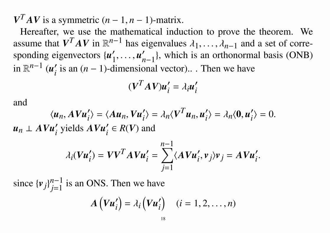
VT AV is a symmetric (n − 1, n − 1)-matrix.Hereafter, we use the mathematical induction to prove the theorem. We
assume that VT AV in Rn−1 has eigenvalues λ1, . . . , λn−1 and a set of corre-sponding eigenvectors u′1, . . . , u
′n−1, which is an orthonormal basis (ONB)
in Rn−1 (u′i is an (n − 1)-dimensional vector).. . Then we have
(VT AV)u′i = λiu′iand
⟨un, AVu′i⟩ = ⟨Aun,Vu′i⟩ = λn⟨VT un,u′i⟩ = λn⟨0,u′i⟩ = 0.un ⊥ AVu′i yields AVu′i ∈ R(V) and
λi(Vu′i) = VVT AVu′i =n−1∑j=1⟨AVu′i , v j⟩v j = AVu′i .
since v jn−1j=1 is an ONS. Then we have
A(Vu′i
)= λi
(Vu′i
)(i = 1, 2, . . . , n)
18

and
⟨Vu′i ,Vu′j⟩ = ⟨VT Vu′i ,u
′j⟩ = ⟨u
′i ,u′j⟩ = δi j, ⟨Vu′i ,un⟩ = 0.
Therefore, λ1, . . . λn, Vu′1, . . .Vu′n−1,un satisfy the condition. QED.
Remark. When λi , λ j, then ⟨ui,u j⟩ = 0.
λi⟨ui,u j⟩ = ⟨Aui,u j⟩ = ⟨ui, AT u j⟩ = ⟨ui, Au j⟩ = λ j⟨ui,u j⟩Then, (λi − λ j)⟨ui,u j⟩ = 0. Therefore, ⟨ui,u j⟩ = 0 if λi , λ j.Remark. When λi = λ j, every linear combination of ui and u j is an eigen-vector.
Since we have Aui = λui and Au j = λu j, for real numbers α and β
A(αui + βu j) = αAui + βAu j = αλui + βλu j = λ(αui + βu j)
Such vectors span an eigenspace.
Let U = (u1 u2 · · · un), we have
UT U = UUT = I,19

UT AU =
λ1 0. . .
0 λn
, A = U
λ1 0. . .
0 λn
UT ,
A =n∑
i=1λiuiuT
i = λ1u1uT1 + · · · + λnunuT
n
(Proof of the last equation)Since ui is an ONB, for any x we can describe x =
∑i⟨x,ui⟩ui. Then,
Ax = A∑
i⟨x,ui⟩ui =
∑i⟨x,ui⟩Aui =
∑iλi⟨x,ui⟩ui
On the other hand, for vectors a and b we have abT x = ⟨x, b⟩a, then, n∑i=1
λiuiuTi
x =∑
iλi⟨x,ui⟩ui = Ax.
QED.
20

2.3.1 Principal component analysis (PCA)Here, the PCA for sample data is explained.
• f1, f2 . . . , f K : samples in RN.• u1,u2 . . . , uN : an ONB.• For an input vector f , the i-th component is given as
⟨ f ,ui⟩ui.
• Choose uiNi=1 such as the sum from the first to M-th components providesthe best approximation of f in the viewpoint of mean square for samples.That is, for any integer M (1 ≤ M ≤ N), minimize
J =K∑
k=1
∥∥∥∥∥∥∥∥M∑i=1⟨ f k,ui⟩ui − f k
∥∥∥∥∥∥∥∥2
(20)
with respect to uiNi=1.• The decomposition by such uiNi=1 is called PCA and uiNi=1 is called a
PCA basis.21
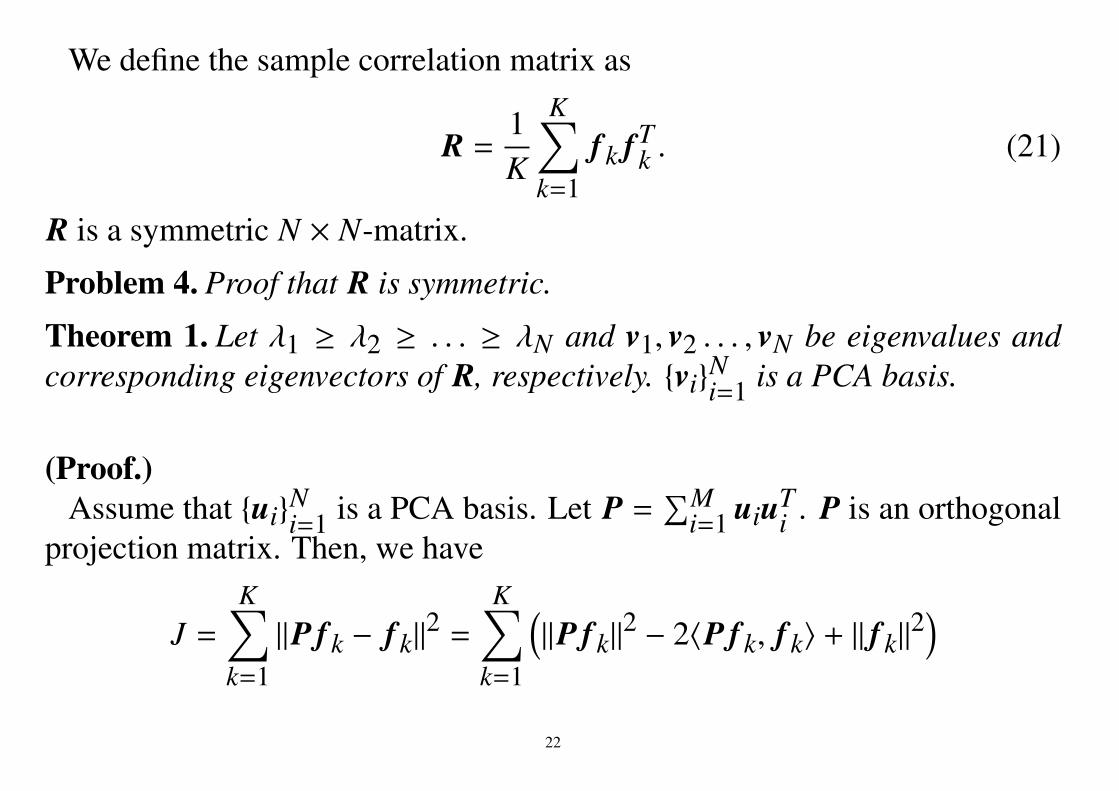
We define the sample correlation matrix as
R =1K
K∑k=1
f k fTk . (21)
R is a symmetric N × N-matrix.
Problem 4. Proof that R is symmetric.
Theorem 1. Let λ1 ≥ λ2 ≥ . . . ≥ λN and v1, v2 . . . , vN be eigenvalues andcorresponding eigenvectors of R, respectively. viNi=1 is a PCA basis.
(Proof.)Assume that uiNi=1 is a PCA basis. Let P =
∑Mi=1 uiuT
i . P is an orthogonalprojection matrix. Then, we have
J =K∑
k=1∥P f k − f k∥2 =
K∑k=1
(∥P f k∥2 − 2⟨P f k, f k⟩ + ∥ f k∥2
)22

=
K∑k=1
(∥P f k∥2 − 2⟨PT P f k, f k⟩ + ∥ f k∥2
)= −
K∑k=1∥P f k∥2 +
K∑k=1∥ f k∥2.
Therefore, we maximize∑K
k=1 ∥P f k∥2. For any vector x, it is clear that
tr(xxT ) = tr
x1x1 x1x2 · · · x1xNx2x1 x2x2 · · · x2xN... ... . . . ...
xN x1 xN x2 · · · xN xN
=N∑
i=1xixi = ∥x∥2.
Then,K∑
k=1∥P f k∥2 =
K∑k=1
tr[(P f k)(P f k)T ] = tr
PK∑
k=1( f k fT
k )PT
= Ktr(PRPT ).
23
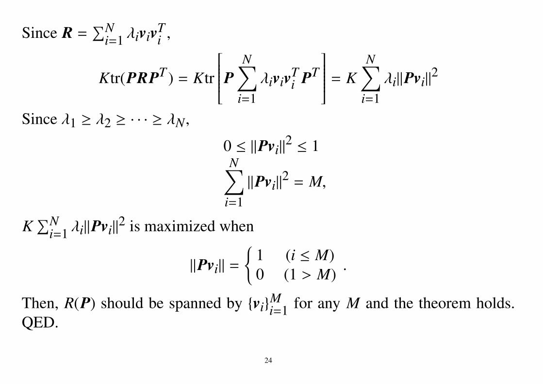
Since R =∑N
i=1 λivivTi ,
Ktr(PRPT ) = Ktr
PN∑
i=1λivivT
i PT
= KN∑
i=1λi∥Pvi∥2
Since λ1 ≥ λ2 ≥ · · · ≥ λN,
0 ≤ ∥Pvi∥2 ≤ 1N∑
i=1∥Pvi∥2 = M,
K∑N
i=1 λi∥Pvi∥2 is maximized when
∥Pvi∥ =
1 (i ≤ M)0 (1 > M) .
Then, R(P) should be spanned by viMi=1 for any M and the theorem holds.QED.
24

2.4 Singular Value Decomposition (SVD)A: (n,m)-matrix (may be non-squared or unsymmetric)
We want to decompose A similarly to the case that A is symmetric. AAT isa symmetric (n, n)-matrix, because
(AAT )T = (AT )T AT = AAT .
Then, AAT has eigenvalues λ1 ≥ λ2 ≥ · · · λn ≥ 0 and corresponding eigen-vectors u1,u2, . . .un such that uini=1 is an ONB. And we have
AAT ui = λiui.
λi ≥ 0 (i = 1, 2, . . . , n) because
λi∥ui∥2 = ⟨λiui,ui⟩ = ⟨AAT ui,ui⟩ = ⟨AT ui, AT ui⟩ = ∥AT ui∥2.Similarly, AT A has eigenvalues µ1 ≥ µ2 ≥ . . . ≥ µm ≥ 0 and corresponding
eigenvectors w1,w2, . . .wm. We have
AT A(AT ui) = AT (AAT ui) = λi AT ui
25

Then, λi and AT ui are eigenvalues and eigenvectors of AT A, respectively.Similarly, µi and Awi are eigenvalues and eigenvectors of AAT , respectively.Then, we have µi = λi for every i = 1, 2, . . . ,min(m, n).
Now we assume that λ1 ≥ λ2 ≥ · · · ≥ λk > 0 and λk+1 = · · · = λn = 0. Let
vi = AT ui/√λi
for i ≤ k and let vimi=k+1 be an arbitrary orthonormal system in the subspacex | AT Ax = 0. Then, for any i ≤ k and any j ≤ k, we have
⟨vi, v j⟩ =⟨
AT ui√λi,
AT u j√λ j
⟩=⟨AAT ui,u j⟩√
λi√λ j
=λi√λi
√λ j⟨ui,u j⟩ = δi j.
As we will prove later, we have x | AT Ax = 0 = x | Ax = 0 = N(A). Itfollows that Avi = 0 for i > k. Then, for any i ≤ k and j > k, we have
⟨vi, v j⟩ = ⟨AT ui/√λi, v j⟩ = ⟨ui/
√λi, Av j⟩ = ⟨ui/
√λi, 0⟩ = 0.
Then, for any i, j ≤ m we have
⟨vi, v j⟩ = δi j.
26

When i ≤ k, the definition of vi and λi > 0 yields that
AT ui =√λivi,
andAvi = AAT ui/
√λi = λiui/
√λi =
√λiui.
We summarize the above as
AT ui =
√λivi (i ≤ min(m, n))
0 (else) , (22)
Avi =
√λiui (i ≤ min(m, n))
0 (else) . (23)
We define (n, n)- and (m,m)-matrices
U = (u1 u2 · · · un) (24)V = (v1 v2 · · · vm) (25)
Since UT U = I and VT V = I, we have
UUT = UT U = I, VVT = VT V = I,27

and
UT AV = UT (Av1 Av2 · · · Avm) =
uT
1uT
2...
uTn
(√λ1u1
√λ2u2 · · ·
√λmin(m,n)umin(m,n) 0 · · · 0)
=
√λ1 0 · · · 0
0√λ2 · · · 0 0
... . . . . . . ...
0 0 · · ·√λmin(m,n)
(m ≥ n)
√λ1 0 · · · 00√λ2 · · · 0
... . . . . . . ...
0 0 · · ·√λmin(m,n)
0
(m < n)
.
28

Then, we have
A = U
√λ1 0 · · · 0
0√λ2 · · · 0 (0)
... . . . . . . ...
0 0 · · ·√λmin(m,n)
(0)
VT , (26)
and
A =k∑
i=1
√λiuivT
i =√λ1u1vT
1 +√λ1u2vT
2 + · · · +√λkukvT
k (27)
(Proof.)
Av j =√λ ju j,
k∑i=1
√λiuivT
i
v j =√λ ju j,
and vimi=0 is an ONB. QED.
29
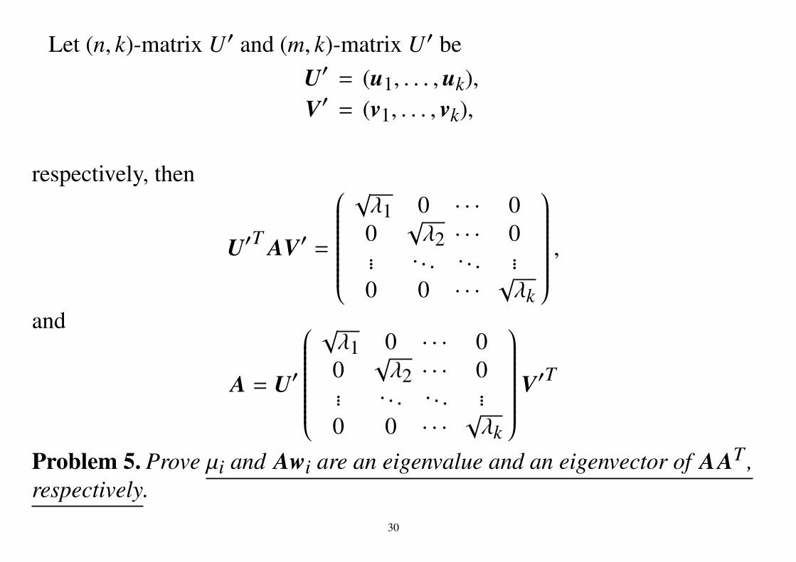
Let (n, k)-matrix U′ and (m, k)-matrix U′ beU′ = (u1, . . . , uk),V′ = (v1, . . . , vk),
respectively, then
U′T AV′ =
√λ1 0 · · · 00√λ2 · · · 0
... . . . . . . ...0 0 · · ·
√λk
,and
A = U′
√λ1 0 · · · 00√λ2 · · · 0
... . . . . . . ...0 0 · · ·
√λk
V′T
Problem 5. Prove µi and Awi are an eigenvalue and an eigenvector of AAT ,respectively.
30

2.5 Generalized Inverses of MatrixFor an (n,m)-matrix A (may not be regular), we define
Type Equation Notation for X1-inverse AX A = A A(1) or A−
2-inverse X AX = X A(2)
3-inverse (AX)T = AX A(3)
4-inverse (X A)T = X A A(4)
Example of other notations :A(1), A(1,2),A† denotes A(1,2,3,4) and called the Moore-Penrose generalized inverse of
A.A1 : the set of all 1-inverse matrices of A.A1, 2 : the set of all 1,2-inverse matrices of A.
31

2.5.1 1-inverseConsider a linear equation
Ax = y. (28)If eq.(28) has a solution (⇔ y ∈ R(A)), it is given as
A−ywith a 1-inverse A− of A.(Proof.)
Since y ∈ R(A), we can let y = Az with a vector z. Then we have
A(A−y) = AA−Az = Az = yQED.
Since(A−A)2 = A−AA−A = A−A,(AA−)2 = AA−AA− = AA−,
then A−A and AA− are projection matrices. QED.32
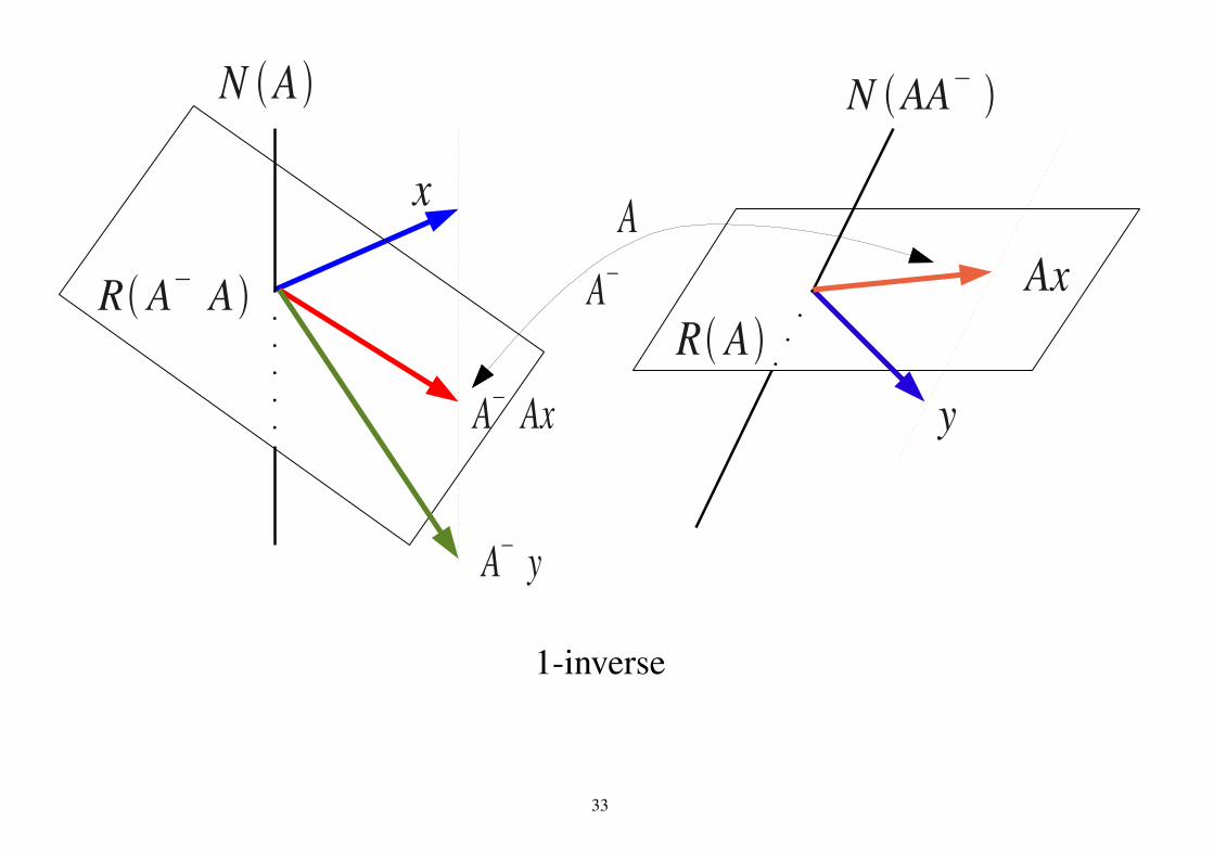
1-inverse
33

In general, 1-inverse matrices are not unique. A general form of 1-inverseis given as
X = A− +W − A−AW AA−. (29)with an arbitrary matrix W.(Proof.)AX A = A(A− +W − A−AW AA−)A = AA−A + AW A − AA−AW AA−A
= A + AW A − AW A = A.For any 1-inverse B of A, let W = B − A−, then we have
X = A− + (B − A−) − A−A(B − A−)AA− = B + A−(A − A)A− = B.It yields that eq.(29) is a general form. QED.
R(A) = R(AA−) (30)N(A) = N(A−A) (31)
(Proof.)R(A) = R(AA−A) ⊂ R(AA−) ⊂ R(A)
34

yields R(A) = R(AA−). Similarly,
N(A) = N(AA−A) ⊃ N(A−A) ⊃ N(A)
QED.
2.5.2 1,2-inverserank(A) = rank(A(1,2))
(Proof.)rank(A) = rank(AA(1,2) A) ≤ rank(A(1,2))
andrank(A(1,2)) = rank(A(1,2) AA(1,2)) ≤ rank(A)
QED.
Lemma 8.
R(A(1,2)) = R(A(1,2) A) (32)N(A(1,2)) = N(AA(1,2)) (33)
35

(Proof of eq.(32).)Since
R(A(1,2)) = R(A(1,2) AA(1,2)) ⊂ R(A(1,2) A) ⊂ R(A(1,2)),
R(A(1,2)) = R(A(1,2) A) holds. Eq.(33) can be proved similarly. QED.
Problem 6. Prove R(AB) ⊂ R(A) and N(AB) ⊃ N(B) for any matrices Aand B.
For any x and y in R(A(1,2)), we have A(1,2) Ax = x and A(1,2) Ay = y. Inthis case, Ax = Ay implies x = y because
y = A(1,2) Ay = A(1,2) Ax = y
Similarly, for any a and b in R(A) such that A(1,2)a = A(1,2)b, we have a = b.Therefore, there is a one-to-one relation between R(A(1,2)) and R(A).
We have the freedom for choosing of R(A(1,2)) and N(A(1,2)).
36

1,2-inverse
37

2.5.3 1,2,3,4-inverse
1,3-inverse: N(AA(1,3)) = R(A)⊥ : minimum mean square errorFor a vector y
∥Ax − y∥ → min. ⇒ x = A(1,3)y
1,4-inverse: R(A(1,4) A) = N(A)⊥ : minimum normFor a vector y ∈ R(A)
∥x∥ → min. ⇒ x = A(1,4)ysubject to Ax = y.
1.2,3,4-inverse has all features: N(A†) = R(A)⊥, R(A†) = N(A)⊥
38

1,3-inverse
39

1,2,3-inverse
40

1,4-inverse
41

1,2,4-inverse
42

1,2,3,4-inverse
43

Theorem 2. 1,2,3,4-inverse is unique.
(Proof.)A†, the 1,2,3,4-inverse of A, satisfies AA†A = A, A†AA† = A†, (AA†)T =
AA†, and (A†A)T = A†A. We define another matrix B that satisfies the sameequations ABA = A, BAB = B, (AB)T = AB, and (BA)T = BA. Then, wehave
B = BAB = BAA†AB = B(A†)T AT BT AT = B(A†)T (ABA)T
= B(A†)T AT = B(AA†)T = BAA† = BAA†AA†
= AT BT AT (A†)T A† = AT (A†)T A† = (A†A)T A† = A†AA† = A†.
QED.
For every y ∈ Rm, there exists x :subject to ∥Ax − y∥ → min.,
∥x∥ → min.
This x is given by x = A†y.44

2.5.4 Calculation of generalized inversesA− : sweep-out method, LU-decomposition
A† :
• Using 1-inverse: A† = AT (AAT )−A(AT A)−AT
• SVD: When
A =k∑
i=1µiuivT
i
with µi , 0 (i = 1, 2, . . . , l), then
A† =k∑
i=1
1µi
viuTi (34)
• Regularization:A† = lim
ε→0AT (AAT + εI)−1 = lim
ε→0(AT A + εI)−1AT
Problem 7. Prove eq.(34). (Examine 1, 2, 3, and 4-inverse conditions.)
45

2.5.5 N(A) = N(AT A)Lemma 9. We have
N(AT A) = N(A), (35)R(AAT ) = R(A). (36)
(Proof.)It is clear that N(AT A) ⊃ N(A). Assume that AT Ax = 0. Then, we have
∥Ax∥2 = ⟨Ax, Ax⟩ = ⟨AT Ax, x⟩ = 0.
∥Ax∥ = 0 yields Ax = 0 and N(AT A) ⊂ N(A). This yields eq.(35).Since we have N(AAT ) = N(AT ) by substituting AT into A, Lemma 5
yields thatR(A) = N(AT )⊥ = N(AAT )⊥ = R(AAT ).
QED.
46

2.6 OctaveTo do the calculation of linear algebra•Make a program by ourselves.• Use packages→ Faster
– Lapack (Linear Algebra PACKage)Linear equation, eigenvalue or singular value decomposition
– BLAS (Basic Linear Algebra Subprograms)Add and multiply matrices
– ATLAS (Automatically Tuned Linear Algebra Software) generates BLAS• Use Octave (or Matlab)→ Easier
– They use the packages for matrix operations→ Faster– Their programming language is realized by interpreter→ Slower
⇒ It is important to understand their feature
Problem 8. Explain about BLAS (You can find the explanation in web).47
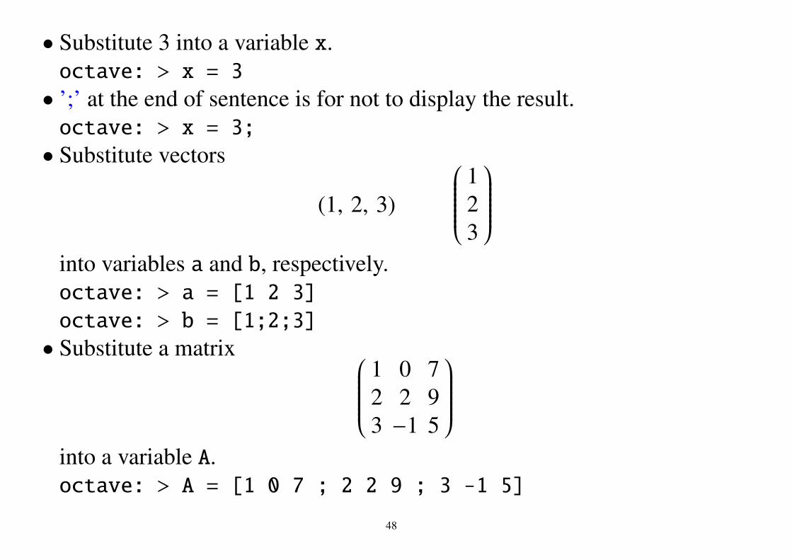
• Substitute 3 into a variable x.octave: > x = 3
• ’;’ at the end of sentence is for not to display the result.octave: > x = 3;
• Substitute vectors
(1, 2, 3)
123
into variables a and b, respectively.octave: > a = [1 2 3]
octave: > b = [1;2;3]
• Substitute a matrix 1 0 72 2 93 −1 5
into a variable A.octave: > A = [1 0 7 ; 2 2 9 ; 3 -1 5]
48
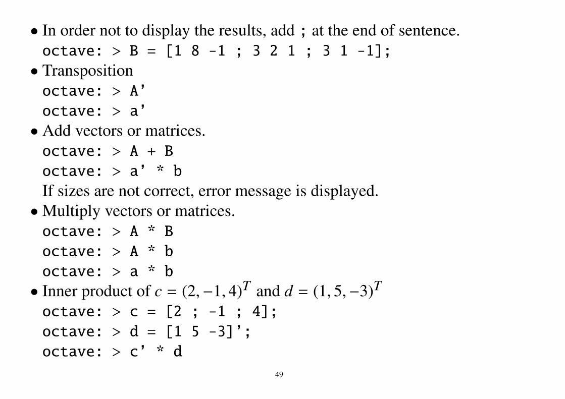
• In order not to display the results, add ; at the end of sentence.octave: > B = [1 8 -1 ; 3 2 1 ; 3 1 -1];
• Transpositionoctave: > A’
octave: > a’
• Add vectors or matrices.octave: > A + B
octave: > a’ * b
If sizes are not correct, error message is displayed.•Multiply vectors or matrices.octave: > A * B
octave: > A * b
octave: > a * b
• Inner product of c = (2,−1, 4)T and d = (1, 5,−3)T
octave: > c = [2 ; -1 ; 4];
octave: > d = [1 5 -3]’;
octave: > c’ * d
49

• X = A−1 is given byoctave: > X = inv(A)
• In order to solve a linear equation Ax = b,octave: > x = A\b
• Check the result.octave: > A * x
• The equation can be solve by using its inverse matrix.octave: > x = inv(A) * b;
A\b is faster than inv(A).•Multiplying or dividing individual elements, that is Ci j = Ai j × Bi j or
Ci j = Ai j/Bi j is given byoctave: > C = A .* B
octave: > C = A ./ B
50

• Add from 1 to 100octave: > sum = 0;
octave: > for i = 1:100
> sum = sum + i;
> end
octave: > sum
•Write the following program in the file yama1.msumm = 0;
for i = 1:100
summ = summ + i;
end
summ
and inputoctave: > yama1
• function : File name : yama3.mfunction [a b] = yama3(c, d, e)
....................................
51

• Etc.– Display by more : more on, more off– Continue the sentence after ’Enter’ : ’...’– Zero matrix : zeros(3), zeros(2,3)– Matrix of which all elements are one : ones(3), ones(2,3)– Size of a matrix : size(A)– Refer/substitute an element of a matrix : A(2,3), A(1,3) = 5– Refer/substitute a part of a matrix :A = [ 1 2 3 4 5 ; 6 7 8 9 10 ; 11 12 13 14 15; ...
16 17 18 19 20]
A(:,2:4)
A(3:4,2:3) = [-1 -2 ; -4 -5 ; -7 -8 ]
– Eigenvalue expansion eig(A)– SVD : svd(A)– Sum : sum(A)– average : mean(a)
52

– variance: var(a)– Norm : norm(a)– Elementary functions : sin(x), cos(x), tan(x), asin(x), acos(x),atan(x), sinh(x), . . ., exp(x), log(x)
– Comment line : %– String : “This is a string.” or ’This is a string.’– File I/O∗ printf∗ fopen∗ fclose∗ fprintf∗ fscanf∗ fread∗ fwrite
• Complex numbers : 1.2 + 3.1i• Use help or Web.
53

2.7 Demo2.7.1 Matrix multiplicationC Program (mmult.c)
#include <math.h>
#include <stdio.h>
double a[1000 * 1000];
double b[1000 * 1000];
double c[1000 * 1000];
main()
int i, j, k, sum, n = 1000;
for (i = 0 ; i < n ; i++)
for (j = 0 ; j < n ; j++)
a[i + n * j] = rand();
b[i + n * j] = rand();
54

printf("Finish set \n");
for (i = 0 ; i < n ; i++)
for (j = 0 ; j < n ; j++)
sum = 0;
for (k = 0 ; k < n ; k++)
sum += a[i + n * k] * b[k + n * j];
c[i + n * j] = sum;
printf("Finish multiplication %f \n", c[0]);
Compile and execute
gcc -O3 mmult.c
./a.out
55
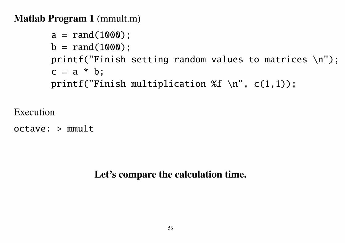
Matlab Program 1 (mmult.m)
a = rand(1000);
b = rand(1000);
printf("Finish setting random values to matrices \n");
c = a * b;
printf("Finish multiplication %f \n", c(1,1));
Execution
octave: > mmult
Let’s compare the calculation time.
56

2.7.2 Image processingInput imageorgImg = imread("barb.jpg");
Display imageimshow(orgImg);
Output imageimwrite(empImg, "empImg.jpg");
3×3 image filter (filter2.m)
OutImage(i, j) =1∑
k=−1
1∑l=−1
A(k, l) InImage(i + k, j + l)
A(k, l) is a filter.1/8 0 -1/82/8 0 -2/81/8 0 -1/8
1/8 2/8 1/80 0 0
-1/8 -2/8 -1/8
0 -1 0-1 4 -10 -1 0
horizontal edge detection vertical edge detection Laplacian57

function out = imgFilter(filter, inImg)
out = zeros(size(inImg));
c = size(inImg, 3);
[yi xi] = size(inImg);
xi = xi/c;
[yf xf] = size(filter);
xfh = floor((xf-1) / 2);
yfh = floor((yf-1) / 2);
extendImg = zeros(yi + yf, xi + xf, c);
extendImg((1+yfh):(yi+yfh), (1+xfh):(xi+xfh),:) = inImg;
58

% Extension
for x = 1:xfh
extendImg((1+yfh):(yi+yfh), x, :) = inImg(:,1,:);
extendImg((1+yfh):(yi+yfh), xi+xf-x,:) = inImg(:,xi,:);
endfor
for y = 1:yfh
extendImg(y, :, :) = extendImg(yfh+1,:,:);
extendImg(yi+yf-y, :, :) = extendImg(yfh+1,:,:);
endfor
for y = 1:yf
for x = 1:xf
out(:,:,:) = out(:,:,:) + filter(y,x) * ...
extendImg((1+yf-y):(yi+yf-y),(1+xf-x):(xi+xf-x),:);
endfor
endfor
59

Example (imgProc.m)
% input image
orgImg = imread("barb.jpg");
% display the input image
figure(1)
imshow(orgImg)
% calculate edge image
divFilt = [0 -1 0 ; -1 4 -1 ; 0 -1 0];
edgeImg = imgFilter(divFilt, orgImg);
% display emphasized image
empImg = edgeImg + orgImg;
empImg = empImg .* (empImg >= 0 & empImg <= 255) ...
+ 255 * (empImg > 255);
60

figure(2)
imshow(empImg);
% display filter image
edgeImg = edgeImg + 128;
edgeImg = edgeImg .* (edgeImg >= 0 & edgeImg <= 255) ...
+ 255 * (edgeImg > 255);
figure(3)
imshow(edgeImg / 255);
imwrite(empImg, "empImg.jpg");
imwrite(edgeImg, "edgeImg.jpg");
61

Original image Edge enhanced image
62

3 Probability3.1 Probability space• Probability is define by using the set theory.
Definition of probability space (V,F , P)V : a set (sample space)F : σ-algebra, that is a set of subsets of V satisfying
1. V ∈ F .
2. If A ∈ F , then V − A ∈ F .
3. If Ai ∈ F , then ∪∞i=1Ai ∈ F .
• A ∈ F is called the ’event’.
63

P : probability measure on F satisfying(Measure is a mapping from a subset to a real number.)
1. P(A) ≥ 0 for every A ∈ F .
2. P(V) = 1.
3. If Ai ∈ F and Ai ∩ A j = ϕ for i , j, then
P(∪∞i=1Ai) =∞∑
i=1P(Ai)
IndependenceTwo event A and B are called independent if and only if
P(A ∩ B) = P(A)P(B)
Conditional distributionThe conditional probability of A under the condition of B is given by
P(A|B) =P(A ∩ B)
P(B)64

Random variable X is a mapping from V to a set of numbers W (integer, realnumbers) such that for any x ∈ W we have
v | X(v) ≤ x ∈ F .In this case, v | X(v) ≤ x is an event.
The cumulative distribution function (CDF) P(x) is defined by
F(x) = P(v ∈ V | X(v) ≤ x).The variable x is called a realized value of a random variable X.
Assume that the range of a random variable X is included in a set of integer.Since v | X(v) = x is an event, probability distribution P(x) is defined by
P(x) = P(v ∈ V | X(v) = x).(The same letter P is used for the measure and probability distribution.)
65

3.2 Random variable of which range is the set of integerExample: (Dice)
V = 1, 2, 3, 4, 5, 6X(v) = v : we can identify V and W.
P(1) = P(1) = F(1) =16
P(1, 2, 3) = F(3) =12
P(ϕ) = 0P(1, 2, 3, 4, 5, 6) = F(6) = 1
P(1, 3, 5|1, 2, 3, 4) = P(1, 3, 5 ∩ 1, 2, 3, 4)P(1, 2, 3, 4) =
P(1, 3)P(1, 2, 3, 4)
=
1323
=12
66

3.3 Random variable of which range is RCDF :
F(x) = P(v ∈ V | X(v) ≤ x).
Probability density function (p.d.f.) : p(x).When there exists a function p(x) such that
p(x)dx = P(v ∈ V | x < X(v) ≤ x + dx = F(x + dx) − F(x) (37)
with the approximation of the first order of dx. We have
p(x) =dF(x)
dx. (38)
(This p.d.f. is not the portable document format)We denote the set v ∈ V | a < X(v) ≤ b by (a, b].Remarks:
(x, x + dx] = (V − (−∞, x]) ∩ (−∞, x + dx],(x, x + dx] should be an event.
67
It is clear that we can handle the probability of V as if V is R.
Expectation of g(x), which is a function on R is defined as.
E[g(X)] =∫R
g(x)dP. (39)
When its density function exists, it is written as
E[g(X)] =∫R
g(x)p(x)dx. (40)
In eq.(39) when P is a probability measure, the definition of integral (it issimplified and we assume g(x) ≥ 0 for brief.) is given as∫
Rg(x)dP = lim
h→0
∞∑l=0
lh · P(x | lh < g(x) ≤ (l + 1)h) (41)
68

Let F is a CDF, the definition of expectation is given as Stieltjes integral.Consider division a = x0 < x1 < x2 < · · · < xn = b and,let ε = maxl=1,2,...,n−1(xl+1 − xl) and ξl ∈ (xl, xl+1).∫
Rg(x)dF = lim
a→−∞ limb→∞
limε→0
n−1∑l=0
g(ξl)F(xl+1) − F(xl)
, (42)
Average (or mean) :
E[X] =∫R
xdP =∫R
xp(x)dx (43)
Variance:
V(X) ≡ E[(X − E[X])2] = E[X2 − 2E[X]X + (E[X])2)]= E[X2] − 2E[X]E[X] + (E[X])2
= E[X2] − (E[X])2 (44)
69

3.4 Two random variables of which range are RConsider two random variables X1(v) and X2(v) from V to R.
For x = (x1, x2) ∈ R2,CDF :
F(x1, x2) = P(v ∈ V | X1(v) ≤ x1, X2(v) ≤ x2)We denote v ∈ V | a1 < X1(v) ≤ b1, a2 < X2(v) ≤ b2 by (a1, b1] × (a2, b2].
(Joint) probability density function (p.d.f.) :When there exists a function p(x1, x2) such that
p(x1, x2)dx1dx2 = P((x1, x1 + dx1] × (x2, x2 + dx2]) (45)
with the approximation of the first order of dx1, dx2. We have
p(x1, x2) =∂2F(x1, x2)∂x1∂x2
. (46)
It is clear that we can handle the probability of V as if V is R2.
70

Marginal distributionCDF of Marginal distributions are defined by
F1(x1) = P(v | X1(v) ≤ x1), (47)F2(x2) = P(v | X2(v) ≤ x2) (48)
and their p.d.f. are defined by
p1(x1) =∂F1(x1)∂x1
=
∫R
p(x1, x2)dx2, (49)
p2(x2) =∂F2(x2)∂x2
=
∫R
p(x1, x2)dx1. (50)
X1 and X2 are said to be independent if and only if
P(v ∈ V | X1(v1) ≤ x1, X2(v2) ≤ x2)= P(v ∈ V | X1(v1) ≤ x1P(v ∈ V | X2(v2) ≤ x2
orF(x1, x2) = F1(x1)F2(x2).
71

By differentiating F(x1, x2) = F1(x1)F2(x2) the condition of independenceby p.d.f. is given as
p(x1, p2) = p1(x1)p2(x2)
Conditional distribution Under the condition that X2 ≤ x2, the probabilityof X1 ≤ x1.
F(x1|x2) =F(x1, x2)F2(x2)
If the probability of X1 ∈ (x1, x1 + dx1] under the condition that X2 ∈(x2, x2 + dx2] can be written as
p(x1|x2)dx1
p(x1|x2) is called the conditional p.d.f. of X1 under the condition that X2 = x2and we have
p(x1|x2) =p(x1, x2)p2(x2)
.
72

Expectation
E[ f (X1, X2)] =∫R
∫R
f (x1, x2)dP =∫R
∫R
f (x1, x2)p(x1, x2)dx1dx2 (51)
Average (or mean) : E[x1] or E[x2]
E[(
X1X2
)]=
(E[X1]E[X2]
)Variance:
E[(X1 − E[X1])2] = E[X21] − (E[X1])2
E[(X2 − E[X2])2] = E[X22] − (E[X2])2
Covariance:
E[(X1 − E[X1])(X2 − E[X2])] = E[X1X2] − E[X1]E[X2]
73

Variance-covariance matrix:
V(X) ≡(
E[(X1 − E[X1])2] E[(X1 − E[X1])(X2 − E[X2])]E[(X2 − E[X2])(X1 − E[X1])] E[(X2 − E[X2])2]
)= E
[((X1 − E[X1])2 (X1 − E[X1])(X2 − E[X2])
(X2 − E[X2])(X1 − E[X1]) (X2 − E[X2])2
)]= E
X21 X1X2
X2X1 X22
− (E[X1]2 E[X1]E[X2]
E[X2]E[X1] E[X2]2
). (52)
Or it can be written by vectors
V(X) = E[(
X1 − E[X1]X2 − E[X2]
)(X1 − E[X1], X2 − E[X2])
]. (53)
Problem 9. Prove eq.(52).
74

3.5 n random variables of which range are RCDF :
F(x1, x2, . . . , xn) = P(v ∈ V | X1(v) ≤ x1, X2(v) ≤ x2, . . . , Xn(v) ≤ xn)We denote v ∈ V | a1 < X1(v) ≤ b1, a2 < X2(v) ≤ b2, . . . , an < Xn(v) ≤ bn
by (a1, b1] × (q2, b2] × · · · × (qn, bn].Probability density function (p.d.f.) :
When there exists a function p(x1, x2, . . . , xn) such that
p(x1, x2, . . . , xn)dx1dx2 . . . dxn= F((x1, x1 + dx1] × (x2, x2 + dx2] × · · · × (xn, xn + dxn]) (54)
with the approximation of the first order of dx1, dx2, . . . , dxn. We have
p(x1, x2, . . . , xn) =∂nF(x1, x2, . . . , xn)∂x1∂x2 . . . ∂xn
. (55)
Marginal and conditional distributions, and independence are defined simi-larly to the case of two random variables.
75

Expectation
E[ f (X1, X2, . . . , Xn)]
=
∫R
∫R· · ·
∫R
f (x1, x2, . . . , xn)dP
=
∫R
∫R
f (x1, x2, . . . , xn)p(x1, x2, . . . , xn)dx1dx2 · · · dxn (56)
Average (or mean) : E[X1] or E[X2] or · · · or E[Xn] or
E
X1X2...
Xn
=
E[X1]E[X2]...
E[Xn]
76

Variance-covariance matrix:
V(X) ≡ E
X1 − E[X1]X2 − E[X2]
...Xn − E[Xn]
(X1 − E[X1], X2 − E[X2], . . . , Xn − E[Xn])
= E
X1X2...
Xn
(X1, X2, . . . , Xn)
− E
X1X2...
Xn
E
[(X1, X2, . . . , Xn)
]
=
E[X1X1] E[X1X2] · · · E[X1Xn]E[X2X1] E[X2X2] · · · E[X2Xn]· · · · · · . . . · · ·
E[XnX1] E[XnX2] · · · E[XnXn]
−
E[X1]E[X1] E[X1]E[X2] · · · E[X1]E[Xn]E[X2]E[X1] E[X2]E[X2] · · · E[X2]E[Xn]· · · · · · . . . · · ·
E[Xn]E[X1] E[Xn]E[X2] · · · E[Xn]E[Xn]
77

3.6 Example of distributionNormal distribution (Section 6)
Successive binary trialsevent S : probability pevent T : probability 1 − p
Binomial distribution (Bernoulli trials)Consider that event S occurs k times in n times trials. The probability isgiven as
nCkpk(1 − p)n−k. (57)
Geometrical distributionAfter the events T occurs k − 1 times continuously, the event S occurs.(TT· · ·TS) The probability is given as
(1 − p)k−1p (58)
78

Pascal distribution At the n-th trail, the k-th event S occurs. The proba-bility is given as
n−1Cn−kpk(1 − p)n−k (59)
Poisson distribution In the binomial distribution, fix np = λ and take limitn→ ∞, then
p(k) = e−λλk
k!. (60)
Beta distributionDistribution of the p-th smallest value among p+q−1 uniform distributionon [0, 1].
p(x) =1
B(p, q)xp−1(1 − x)q−1, (61)
where
B(p, q) =∫ 1
0xp−1(1 − x)q−1dx. (62)
79

Exponential distributionp(x) = λe−λx. (63)
Gamma distributionSum of exponential distribution.Standard gamma distribution is given by
p(x) =1Γ(γ)
xγ−1e−x. (64)
Gamma functionΓ(γ) =
∫ ∞0
tγ−1etdt (65)
(Γ(n) = (n − 1)! when n is an integer.)
80
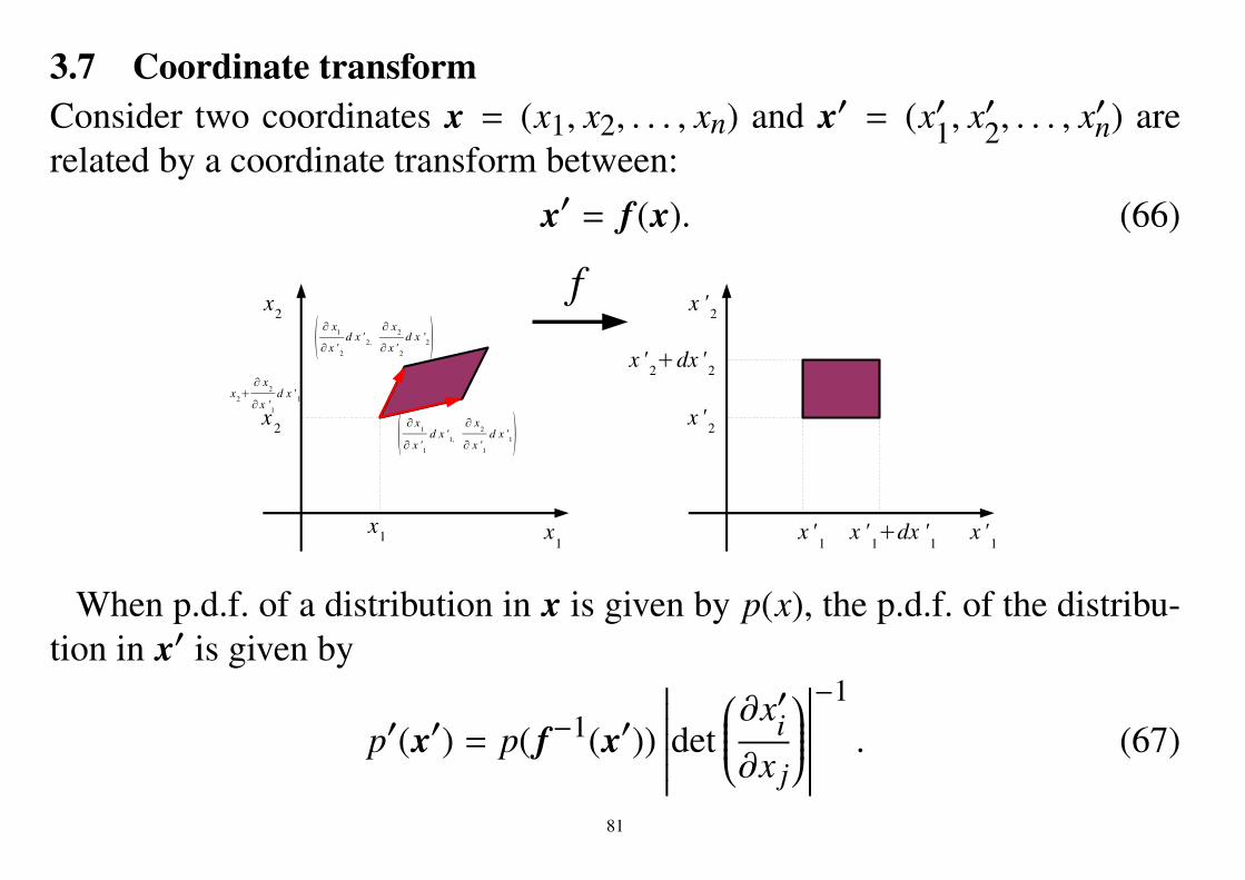
3.7 Coordinate transformConsider two coordinates x = (x1, x2, . . . , xn) and x′ = (x′1, x′2, . . . , x′n) arerelated by a coordinate transform between:
x′ = f (x). (66)
When p.d.f. of a distribution in x is given by p(x), the p.d.f. of the distribu-tion in x′ is given by
p′(x′) = p( f−1(x′))
∣∣∣∣∣∣∣det∂x′i∂x j
∣∣∣∣∣∣∣−1
. (67)
81

(Proof.)
p′(x′)dx′1dx′2 · · · dx′n= P(x′ | x′ ∈ [x′1, x
′1 + dx′1] × [x′2, x′2 + dx′2] × · · · × [x′n, x
′n + dx′n])
= P(x | f (x) ∈ [x′1, x′1 + dx′1] × [x′2, x′2 + dx′2] × · · · × [x′n, x′n + dx′n])
= P(
f−1([x′1, x′1 + dx′1] × [x′2, x′2 + dx′2] × · · · × [x′n, x′n + dx′n]))
= p( f−1(x′))
·volume of
(∂ fi∂x j
)−1([x′1, x′1 + dx′1] × [x′2, x′2 + dx′2] × · · · × [x′n, x′n + dx′n])
= p( f−1(x′))
∣∣∣∣∣∣det(∂ fi∂x j
)∣∣∣∣∣∣−1dx′1dx′2 · · · dx′n.
QED.
Remark: ∂ fi∂x j
is the Jacobian matrix.
82

Consider a two-dimensional random variable (X1, X2) and its p.d.f is givenby p(x1, x2). Assume that the random variable Y is given by
Y = X1 + X2.
Let q(y) be the p.d.f. of Y . Then, we have
q(y) =∫ ∞−∞
p(x1, y − x1)dx1 =
∫ ∞−∞
p(y − x2, x2)dx2. (68)
83

(Proof.) Consider a coordinate Transform:
y = x1 + x2,
x2 = x2.
det
∂y∂x1
∂y∂x2
∂x2∂x1
∂x2∂x2
= det(
1 10 1
)= 1.
Then, we havedydx2 = dx1dx2.
(This equality implies the area of the small parallelogram is dydx2).Let p1(y, x2) be the p.d.f. of joint distribution of y and x2. Since q(y) is given
by the marginal distribution of p1(y, x2) = p(x1, x2),
q(y) =∫ ∞−∞
p1(y, x2)dx2 =
∫ ∞−∞
p(y − x2, x2)dx2.
QED.84
4 Normal distributionThe normal distribution is the mostly used distribution.
• Observation error• Processing error• Result of examination
Gaussian function :p(x) =
1√
2πe−x2/2.
We will provide characterizations of the normal distribution.
Problem 10. Explain an application where the normal distribution is used.
85

4.1 Probability density function of normal distribution1-dimensional standard normal distribution
p(x) =1√
2πe−x2/2. (69)
1-dimensional normal distribution
p(x) =1
√2π|σ|
e−(x−µ)2/2σ2. (70)
n-dimensional multivariate normal distribution
p(x) =1
√(2π)n
e−(x21+x2
2+···+x2n)/2=
1√
(2π)ne−∥x∥
2/2. (71)
n-dimensional multivariate normal distribution
p(x) =1
√(2π)n|Σ|
e−⟨x−µ,Σ−1(x−µ)⟩/2. (72)
86

4.2 Gauss distributionLet p(x; µ) be a p.d.f. on R with a parameter µ ∈ R.
(i) The p.d.f. p(x; µ) depends on only x − µ. That is,
p(x; µ) = p(x − µ). (73)
(ii) The most likelihood estimator of µ is given as the average of sample data.(We assume that sample date are independent.)
Then, with σ > 0 we have
p(x; µ) =1√
2πe−(x−µ)2/2σ2
. (74)
(Proof.)Let X = (X1, X2, . . . , Xn) is sampled date. The likelihood is given as
L(X; µ) = p(X1; µ)p(X2; µ) · · · p(Xn; µ). (75)
87

The most likelihood estimator µ is the µ which maximizes L(X; µ). Condition(ii) implies
µ =1n
n∑i=1
Xi. (76)
The assumption is described as for any x = (x1, x2, . . . , xn)
0 =∂L(x; µ)∂µ
∣∣∣∣∣∣µ=µ
=∂
∂µp(x1 − µ) · · · p(xn − µ)
∣∣∣∣∣∣µ=µ
= −L(x; µ)n∑
i=1
p′(xi − µ)p(xi − µ)
∣∣∣∣∣∣∣∣µ=µ
,
where we redefine µ = 1n∑n
i=1 xi. Then we haven∑
i=1
p′(xi − µ)p(xi − µ)
= 0. (77)
88

Let
ti = xi − µ = xi −1n
n∑j=1
x j.
It is clear thatn∑
i=1ti = 0,
andn∑
i=1
p′(ti)p(ti)
= 0.
Lemma 10. If a differentiable function f (t) satisfies that∑n
i=1 f (ti) = 0 forany ti such that
∑ni=1 ti = 0, then f (t) = at with a constant a.
89

(Proof.)It follows that f (−t2 − t3) + f (t2) + f (t3) = 0. Differentiate the equation by
t3, and we have− f ′(−t2 − t3) + f ′(t3) = 0.
Let t2 = −t3, for any t3 we have
f ′(t3) = f ′(0) = const = a.
Then,f (t) = at + b
with a constant b. We have
f (−t2 − t3) + f (t2) + f (t3) = 3b = 0.
This completes the proof. QED.
90

From Lemma 4, we havep′(t)p(t)= at,
and it yields that
log p(t) =12
at2 + c.
Then, we havep(t) = e
12at2+c,
andp(t) = e
12at2+c.
Let σ2 = −1/a and∫ ∞−∞ p(x; µ)dx = 1 yields that
p(x; µ) = p(x − µ) =1√
2πσe−(x−µ)2/2σ2
.
QED.
91

4.3 Maxwell distributionMaxwell distribution is the velocity distribution of ideal gas.
Let’s consider two independent random variables X1 and X2. Their p.d.f. isdenoted by pX(x1, x2). For θ , 0,±π2,±π, . . ., we define two random variablesby linear combinations of X1 and X2 as
Y1 = X1 cos θ + X2 sin θ, (78)Y2 = −X1 sin θ + X2 cos θ. (79)
Their p.d.f. is denoted by pY(y1, y2). We assume that the random variables Y1and Y2 are independent. Then, the distribution of X1 and X2 should be normal.
Since the transform is a rotation, we have
pX(x1, x2) = pY(y1, y2). (80)
Since the distribution is also independent with respect to Y1 and Y2, we have
pX(x1, x2) = a(x1)b(x2),pY(y1, y2) = c(y1)d(y2).
92

where a, b, c, d are functions. It is clear that∂
∂x1∂x2log pX = 0, (81)
∂
∂y1∂y2log pY = 0. (82)
We have∂
∂y1=∂x1∂y1
∂
∂x1+∂x2∂y1
∂
∂x2= cos θ
∂
∂x1− sin θ
∂
∂x2,
∂
∂y2=∂x1∂y2
∂
∂x1+∂x2∂y2
∂
∂x2= sin θ
∂
∂x1+ cos θ
∂
∂x2It follows that
0 =∂
∂y1
∂
∂y2log pY
= sin θ cos θ
∂2
∂x21
− ∂2
∂x22
log pX + (cos2 θ − sin2 θ)∂
∂x1∂x2log pX
93

= sin θ cos θ
∂2
∂x21
− ∂2
∂x22
log pX. (83)
From eq.(81) we have
d2
d2x1log a(x1) =
d2
d2x2log b(x2) = α = const.
By integrating the equation, we have
log a(x1) = αx21 + β1x1 + γ1,
log b(x2) = αx22 + β2x2 + γ2,
andpX(x1, x2) = eα(x2
1+x22)+β1x1+β2x2+γ1+γ2.
It is clear that we can describe the expression as
p(x1, x2) =1
2πσ2e−(x1−µ1)2+(x2−µ2)2/2σ2. (84)
94
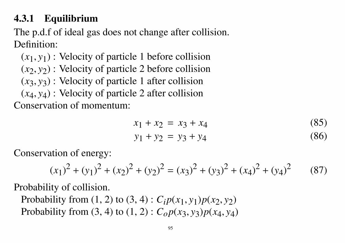
4.3.1 EquilibriumThe p.d.f of ideal gas does not change after collision.Definition:
(x1, y1) : Velocity of particle 1 before collision(x2, y2) : Velocity of particle 2 before collision(x3, y3) : Velocity of particle 1 after collision(x4, y4) : Velocity of particle 2 after collision
Conservation of momentum:
x1 + x2 = x3 + x4 (85)y1 + y2 = y3 + y4 (86)
Conservation of energy:
(x1)2 + (y1)2 + (x2)2 + (y2)2 = (x3)2 + (y3)2 + (x4)2 + (y4)2 (87)
Probability of collision.Probability from (1, 2) to (3, 4) : Cip(x1, y1)p(x2, y2)Probability from (3, 4) to (1, 2) : Cop(x3, y3)p(x4, y4)
95

Since the mutual speed is the same between (1, 2) and (3, 4), we haveCi = Co.
Then equilibrium is express byp(x1, y1)p(x2, y2) = p(x3, y3)p(x4, y4). (88)
for any x1, y1, x2, y2, x3, y3, x4, y4 that satisfy conservation law. For small dxand dy, let x1 = x + dx, x2 = x, x3 = x + dx, x4 = x, y1 = y + dy, y2 = y,y3 = y, and y4 = y + dy. Since it is clear that such xi, yi (i = 1, 2, 3, 4) satisfyconservation law, eq.(88) has to hold.
p(x + dx, y + dy)p(x, y) = p(x + dx, y)p(x, y + dy) (89)By Taylor expansion until second order, we havep +
∂p∂x
dx +∂p∂y
dy +12∂2p∂x2 (dx)2 +
∂2p∂x∂y
(dx)(dy) +12∂2p∂y2 (dy)2
p
=
p +∂p∂x
dx +12∂2p∂x2 (dx)2
p +∂p∂y
dy +12∂2p∂y2 (dy)2
.96

In the equation, the 0-th and the first order terms are vanished. The remainedsecond order terms are given by ∂2p
∂x∂y− ∂p∂x∂p∂y
dxdy = 0.
Then, we have∂2p∂x∂y
− ∂p∂x∂p∂y= 0 (90)
From the equation, we have
∂
∂x∂
∂ylog p =
∂
∂x
(1p∂p∂y
)=
1p2
∂2p∂x∂y
− ∂p∂x∂p∂y
= 0.
so that eqs.(81) and (82) hold since equilibrium does not depend on the coor-dinates. Therefore p(x, y) has to be normal.
Conversely, the probability is normal, from conservation of energy, it is clearthat eq. (88) holds.
97

4.4 Maxwell-Boltzmann distribution4.4.1 Boltzmann distributionDefinition :
n : the number of particlesm : the number of boxesεi : the energy of the box iε : the total energyni : the number of particles in the box i
Assume that we can distinguish each particle. When we fix ni for each box,the number of cases G is given as
G =n!
n1!n2! . . . nM!. (91)
We maximize G under the condition that the total number of particles and the
98

total energy are fixed. Then, maximize G subject toM∑
i=1ni = n, (92)
M∑i=1
εini = ε. (93)
The Stirling’s asymptotic formula is given as
log n! ≃ n(log n − 1). (94)
By using this formula, we have
log G ≃ n(log n − 1) −m∑
i=1ni(log ni − 1) = n log n −
m∑i=1
ni log ni.
We use Lagrange’s method.
J = n log n −M∑
i=1ni log ni + α
n − M∑i=1
ni
+ βε − M∑
i=1εini
. (95)
99

By differentiating J with ni, we have
0 =∂J∂ni= − log ni − 1 − α − βεi.
Then,ni = e−βεi−α−1, (96)
where α and β are decided by eqs.(92) and (93).
4.4.2 Maxwell-Boltzmann distributionSince energy is often given by a squared term such as εi ∼ v2
i , we have
ni = e−βv2i −α−1. (97)
It implies the normal distribution.
100

4.4.3 Maximum entropyMaximize the following entropy of the p.d.f. p(x)∫ ∞
−∞p(x) log p(x)dx (98)
under the conditions that its variance is constant∫ ∞−∞
x2p(x)dx = σ2, (99)
and p(x) is a p.d.f. ∫ ∞−∞
p(x)dx = 1. (100)
By using the Lagrange’s method, we can obtain .
p(x) =1√
2πσe−x2/2σ2
.
101

4.5 Central limit theoremDefinition:
pX(x) : an arbitrary p.d.f. (with some conditions).X1, X2, . . . , Xn : independently sampled data from pX(x).µ : its average (=
∫xpX(x)dx)
σ2 : its variance (=∫
(x − µ)2pX(x)dx)
Consider a random variable Y given by
Y =X1 + X2 + · · · Xn − nµ
√nσ
. (101)
It converges to a standard normal distribution when n → ∞. (’Standard’means that its average and variance are 0 and 1, respectively.)
p(y) =1√
2πe−y2/2 (102)
102

Characteristic function (Fourier transform of p.d.f.)The characteristic function ϕX(ω) of p(x) is defined as
ϕX(ω) =∫ ∞−∞
eiωxp(x)dx. (103)
We have
E[Xn] = (−i)n dn
dωnϕX(ω)
∣∣∣∣∣∣ω=0
. (104)
(Proof.)
dn
dωnϕX(ω)
∣∣∣∣∣∣ω=0=
∫ ∞−∞
(dn
dωneiωx)
p(x)dx
∣∣∣∣∣∣ω=0= (i)n
∫ ∞−∞
xneiωxp(x)dx
∣∣∣∣∣∣ω=0
= (i)n∫ ∞−∞
xnp(x)dx
= (i)nE[Xn]
QED.103

When Y = X1 + X2, we have
pY(y) =∫
pX1(y − x)pX2(x)dx
andϕY(ω) = ϕX1(ω) · ϕX2(ω).
LetZ =
X − µ√
nσ. (105)
Then,pZ(z) =
√nσpX(
√nσz + µ). (106)
We have
µZ = E[Z] =E[X] − µ√
nσ= 0, (107)
σ2Z = E[Z2] =
E[(X − µ)2]nσ2 =
1n. (108)
104

The Taylor expansion of ϕZ(ω) yields that
ϕZ(ω) = ϕZ(0) +dϕZdω
∣∣∣∣∣ω=0
ω +12!
dϕZdω
∣∣∣∣∣ω=0
ω2 + · · · (109)
= ϕZ(0) + iE[Z]ω +i2
2!E[Z2]ω2 + · · · (110)
= 1 + i0ω − 12nω2 + · · ·
= 1 − 12nω2 + · · · . (111)
SinceY = Z1 + Z2 + · · · + Zn,
we have
ϕY(ω) = [ϕZ(ω)]n =
1 − ω2
2n+ ω3O(n−3/2)
n
.
Sincelim
n→∞
(1 +
xn
)n= ex,
105

we havelim
n→∞ ϕY(ω) = e−ω2/2. (112)
This is a characteristic function for the standard normal distribution. Sincethe Fourier transform of a Gauss function is given by a Gauss function, thecentral limit theorem was proved.
4.6 Limit of Binomial distributionIts probability is given as
nCkpk(1 − p)n−k. (113)
When n is very large, it is approximated by the normal distribution of whichaverage is np and variance is np(1 − p) (Laplace’s theorem).
106
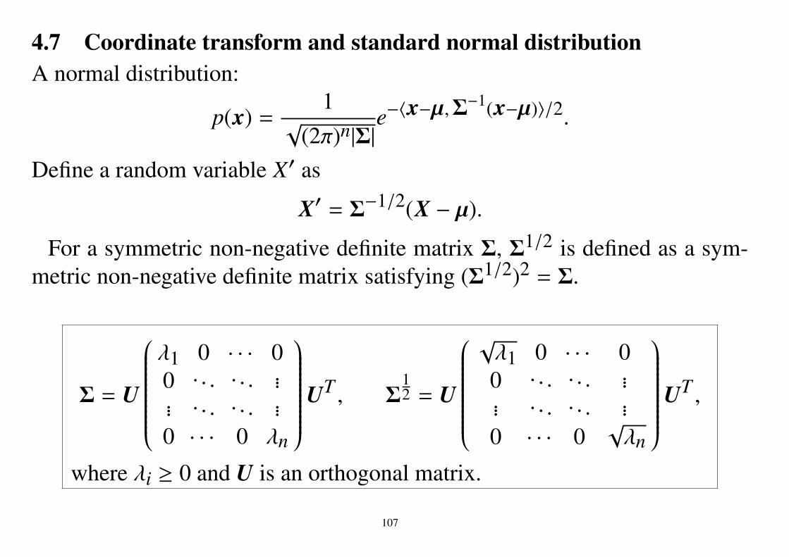
4.7 Coordinate transform and standard normal distributionA normal distribution:
p(x) =1
√(2π)n|Σ|
e−⟨x−µ,Σ−1(x−µ)⟩/2.
Define a random variable X′ as
X′ = Σ−1/2(X − µ).
For a symmetric non-negative definite matrix Σ, Σ1/2 is defined as a sym-metric non-negative definite matrix satisfying (Σ1/2)2 = Σ.
Σ = U
λ1 0 · · · 00 . . . . . . ...... . . . . . . ...0 · · · 0 λn
UT , Σ12 = U
√λ1 0 · · · 00 . . . . . . ...... . . . . . . ...
0 · · · 0√λn
UT ,
where λi ≥ 0 and U is an orthogonal matrix.
107

We haveX = Σ1/2X′ + µ,
∂x′i∂x j= Σ−1/2.
Then, the standard normal density function
p′(x′) = | det(Σ−1/2)|−1p(Σ1/2x′ + µ) =1
√(2π)n
e−∥x′∥2/2 (114)
is derived from the coordinate transform.
Mahalanobis distance : Distance in the transformed space is measured bythe vectors of original space as
d(x, y) = ⟨x − y,Σ−1(x − y)⟩
Problem 11. Prove det(Σ
12
)=√
det(Σ) =√λ1λ2 · · · λn.
108

4.8 Distributions related to normal distribution4.8.1 χ2-distributionLet X1, X2, . . . Xr be random variables of independent standard normal distri-butions. χ2 distribution of r degree of freedom is a distribution of
X = X21 + X2
2 + · · · + X2r . (115)
Its p.d.f. is given as
pχ2r(x) =
12r/2Γ(r/2)
xr1−1e−
x2, (116)
where Γ(a) =∫ ∞0 xa−1e−xdx. (Γ(n) = (n − 1)!)
Properties:
E[X] = r,V[X] = 2r,
argmaxx pχ2r(x) = r − 2.
109

Theorem 3. (Cochran’s theorem)X1, X2, . . . , Xn : random variables of independent standard normal distri-
butions.Y1,Y2, . . . , Ym : random variables of independent standard normal distri-
butions which are given by linear combinations of X1, X2, . . . , Xn as Y1...
Ym
= A
X1...
Xn
,where A is an (m, n)-matrix. Then,
X21 + X2
2 + · · · + X2n − (Y2
1 + Y22 + · · · + Y2
m)
is a χ2-distribution of (n − m) degree of freedom.
110

ExampleLet X1, X2, . . . , Xn be independent samples of a standard normal distribution
of the average m and the variance σ2 (N(µ, σ2)). Let
µ =1n
n∑i=1
Xi. (117)
The distribution of µ is given as N(µ, σ2/n).
1σ2
n∑i=1
(Xi − µ)2
=1σ2
n∑i=1
[(Xi − µ) − (µ − µ)
]2=
1σ2
n∑i=1
(Xi − µ) − 1n
n∑j=1
(X j − µ)
2
111

=1σ2
n∑i=1
(Xi − µ)2 − 2n
n∑i=1
n∑j=1
(Xi − µ)(X j − µ) +1n
n∑i=1
(Xi − µ)
2
=
n∑i=1
(Xi − µσ
)2−
n∑i=1
Xi − µσ√
n
2
.
Since
(Xi − µ)/σ : N(0, 1), (118)n∑
i=1(Xi − µ)/σ
√n : N(0, 1). (119)
And∑n
i=1(Xi − µ)/σ√
n is an linear combination of (Xi − µ)/σ.
⇒We can use Cochran’s theorem.
112

Then, 1σ2
∑ni=1(Xi − µ)2 is a χ2-distribution of n− 1 degrees of freedom. We
have
E
1σ2
n∑i=1
(Xi − µ)2
= n − 1.
An estimator of σ2 is given as
σ2 =1
n − 1
n∑i=1
(Xi − µ)2. (120)
This is an unbiased estimator ofσ2. That is, the average of estimator coincideswith the true value.
E[σ2] = E
1n − 1
n∑i=1
(Xi − µ)2
= σ2
n − 1E
1σ2
n∑i=1
(Xi − µ)2
(121)
=σ2
n − 1(n − 1) = σ2 (122)
113

4.9 F-distributionDefinition
S 1 : the random variable of χ2-distribution of d1 degrees of freedom.S 2 : the random variable of χ2-distribution of d2 degrees of freedom.
S 1 = X21 + X2
2 + · · · + X2d1
S 2 = Y21 + Y2
2 + · · · + Y2d2
where X1, . . . , Xd1 and Y1, . . . , Yd2 are independent random variables of nor-mal distributions.
F : a random variable (F(d1, d2)-distribution) defined as
F =
S 1d1S 2d2
Its p.d.f. is given by (B(x, y) is the beta function)
pF(x) =1
xB(d1/2, d1/2)
(d1x
d1x + d2
)d1/2 (1 − d1x
d1x + d2
)d2/2
114

4.10 t-distribution (student distribution)Definition
Xi (i = 1, 2, . . . , n) : random variables of a normal distributionµ : the average of the normal distributionσ2 : the variance of the normal distributionX and σ2 are defined as
X =1n
n∑i=1
Xi, σ2 =1
n − 1
n∑i=1
(Xi − X)2
T : a random variable (T -distribution) defined as
T =X − µσ
√n
Its p.d.f. is given by
pT (x) =Γ(ν + 1)/2√νπ Γ(ν/2)
(1 + t2/ν)(v+1)/2
where v = n − 1 (degree of freedom).115

5 Test5.1 Example (two-side test)• p : The probability that the front of a coin appears.• Hypothesis : p = 1/2.• Toss the coin 20 times.• The front appears 15 times. ⇒ Is the hypothesis correct?• If the hypothesis is correct, its probability is
20C15
(12
)15 (12
)5≃ 0.015.
• Since the probability is very low, hypothesis does not seem to be correct.• In statistics this is called test.• If we assume that the appearance of 15 times front implies the hypothesis
is incorrect, those of 16, 17, 19, and 20 times also.•We evaluate the probability not of 15 times but of not less than 15 times.• Furthermore, when its back appears not less than 15 times, we should as-
sume that the hypothesis is incorrect as well.116

• The probability that the front or the back appears not less than 15 times is
2 × (20C15 +20 C16 +20 C17 +20 C18 +20 C19 +20 C20)(12
)20= 0.0414
Octave function: k = 15
binocdf(20 - k, 20, 1.0 - 0.5) + binocdf(20 - k, 20, 0.5)
• p-value : The probability of the region where we should reject the hypoth-esis if we do it for the sample data.
k 20 19 18 17 16p-value 1.91 × 10⁻⁶ 4.01 × 10⁻⁵ 4.02 × 10⁻⁴ 2.58 × 10⁻³ 1.18 × 10⁻²
15 14 13 12 11 104.14 × 10⁻² 1.15 × 10⁻¹ 2.63 × 10⁻¹ 5.03 × 10⁻¹ 8.24 × 10⁻¹ 1.0• Significance level : It p-value is less than the significance level, the hy-
pothesis is rejected.• The hypothesis p = 1/2 is rejected at significance level 0.05.• The hypothesis p = 1/2 is not rejected at significance level 0.01.
117

5.2 Example (one-side test)• p : the probability of a defective product• Hypothesis : p = 1/1000. (or less)• For 10000 productions, we found 17 defective products.• The probability that not less than 17 defective products are produced is
given by CDF of the binomial distribution.binocdf(10000 - 17, 10000, 1.0 - 0.001) = 0.026977
• The hypothesis p = 1/1000 is rejected at significance level 0.05.• The hypothesis p = 1/1000 is not rejected at significance level 0.01.• In this case we do not consider the opposite side.• For example, assume that we could not find any defective product.• Even if it is rare from the hypothesis p = 1/1000 and p should be smaller,
we do not reject the hypothesis.•When p should be larger, the hypothesis is rejected.binocdf(10000 - 17, 10000, 1.0 - 0.0011) = 0.055823
then the hypothesis p = 1.1/1000 is not rejected at significance level 0.05.
118

Problem 12. Fill the three ?.binocdf(x, n, p) = 1.0 - binocdf(?, ?, ?)
5.3 Critical region• Critical region : the region of which probability coincides with the signifi-
cance level and where the hypothesis should be rejected.• For the first example (two-side test), let K and µ be the number of appear-
ance of front and its average. Here, µ = 10. Then the critical region ofsignificance level 0.05 is given by
|K − µ| ≥ 5.
p-value = 0.041389 for |K − µ| ≥ 5.p-value = 0.11532 for |K − µ| ≥ 4.
• For the second example (one-side test), the critical region of significancelevel 0.05 is given by
K ≥ 16.Its p-value is 0.048654.
119

5.4 Power• Null hypothesis : Hypothesis may be rejected. (Ex. p = 1/2))• Alternative hypothesis : the negation of the null hypothesis. (Ex. p , 1/2))• p-value is calculated by using the null hypothesis.• Power : The probability that the null hypothesis is rejected, when it is not
correct. It depends on p.• Power function : power for given parameters. (Ex. of parameter: p).• For the first example, let the significance level be 0.05. When the front
appears not more than 5 or not less than 15 times (|K − µ| ≥ 5), the nullhypothesis is rejected.• Then its probabitly if given by using the CDF of binomial distribution.
Octave description: binocdf(5, 20, p) + binocdf(5, 20, 1-p)
p 0.0 or 1.0 0.1 or 0.9 0.2 or 0.8 0.3 or 0.7 0.4 or 0.6 0.5power 1.0 0.98875 0.80421 0.41641 0.12721 0.041389
Even if p = 0.5, the hypothesis p = 0.5 is rejected with probability 0.041389.
120

5.5 Number of trials•When the number of trials n is very large, the binomial distribution can be
approximated by the normal distribution:Average : µ = npVariance : σ2 = np(1 − p)P.d.f.:
p(k) =1√
2πσe−(k−µ)2
2σ2
•Meaning : for 0 ≪ m ≪ k, the probabity that the front appears from k tok + m − 1 times is approximately given by p(k)m.• The transformed random variable
X =K − µσ
expresses the standard normal distribution approximately.
121

• Let µ0 and σ0 be µ and σ when p = 1/2, respectively.
µo = 0.5nσo = 0.5
√n
• The critical region for significance level α can be described by
|X| = |K − µo|σ0
≥ xα/2.
• xα/2 is given by ∫ ∞xα/2
1√
2πe−x2/2dx = α/2.
•When α = 0.05, xα/2 ≃ 1.96.• The previous relation can be shown by the following equation.∫ µ0−σ0xα/2
−∞
1√2πσ0
e−(k−µ0)2
2σ20 dk +
∫ ∞µ0+σ0xα/2
1√
2πσ0e−(k−µ0)2
2σ20 dk = α.
122

• The value of the power function at p is given by∫ µ0−σ0xα/2
−∞p(k)dk +
∫ ∞µ0+σ0xα/2
p(k)dk
=
∫ µ0−σ0xα/2
−∞
1√
2πσe−(k−µ)2
2σ2 dk +∫ ∞µ0+σ0xα/2
1√
2πσ0e−(k−µ)2
2σ2 dk
=
∫ µ0−µ−σ0xα/2σ
−∞
1√
2πe−x2/2dx +
∫ ∞µ0−µ+σ0xα/2
σ
1√
2πe−x2/2dx
=
∫ µ0−µ−σ0xα/2σ
−∞
1√
2πe−x2/2dx +
∫ −µ0−µ+σ0xα/2
σ
−∞
1√
2πe−x2/2dx
• The power function for significance level 0.05 and p = 0.6:n 20 100 200 260 300 400 500power 0.14019 0.51631 0.81228 0.90165 0.93762 0.98133 0.99483
•When p = 0.6 and we have 260 trials, the probability that we can rejectp = 0.5 at significance level 0.05 is 0.90165.
123

Octave commands for power function
n = 260
p = 0.6
xa = 1.96
mu0 = 0.5 * n;
mu = p * n;
sigma0 = 0.5 * sqrt(n);
sigma = sqrt(p * (1-p) * n);
normcdf((mu0 - mu - sigma0 * xa) /sigma) ...
+ normcdf((mu - mu0 - sigma0 * xa) /sigma)
Octave functionsBeta Distr. betapdf betacdf
Binomial Distr. binopdf binocdf
Cauchy Distr. cauchy_pdf cauchy_cdf
Chi-Square Distr. chi2pdf chi2cdf
Univariate Discrete Distr. discrete_pdf discrete_cdf
124

Empirical Distr. empirical_pdf empirical_cdf
Exponential Distr. exppdf expcdf
F-Distr. fpdf fcdf
Gamma Distr. gampdf gamcdf
Geometric Distr. geopdf geocdf
Hypergeometric Distr. hygepdf hygecdf
Kolmogorov Smirnov Distr. N.A. kolmogorov_smirnov_cdf
Laplace Distr. laplace_pdf laplace_cdf
Logistic Distr. logistic_pdf logistic_cdf
Log-Normal Distr. lognpdf logncdf
Pascal Distr. nbinpdf nbincdf
Univariate Normal Distr. normpdf normcdf
Poisson Distr. poisspdf poisscdf
t- (Student) Distr. tpdf tcdf
Univariate Discrete Distr. unidpdf unidcdf
Uniform Distr. unifpdf unifcdf
Weibull Distr. wblpdf wblcdf125

5.6 Theory of test5.6.1 Most powerful test• p(x; θ) is a p.d.f of X with a parameter θ.• The null hypothesis : θ = θ0• wα : the critical region for the significance level α.
P(X ∈ wα; θ0) ≤ α• The power when θ = θ1(, θ0) is given by
L(θ1) = P(X ∈ wα; θ1)
•We would like to maximize L(θ1) with respect to wα.• Test function :
ϕ(x) =
1 (x ∈ wα)0 (x < wα)
• For probabilistic test, we consider ϕ(x) is a function such that 0 ≤ ϕ(x) ≤ 1.• Probabilistic test : the hypothesis is rejected probabilistically for the same
sample x. The value of ϕ(x) is the rejection rate for x.
126

• The problem is that maximize the power∫ϕ(x)p(x; θ1)dx (123)
under the condition that ∫ϕ(x)p(x; θ0)dx = α. (124)
•With a parameter λ, we have∫ϕ(x)p(x; θ1)dx =
∫ϕ(x)
[p(x; θ1) − λp(x; θ0)
]dx + λα.
• This is maximized when
ϕ(x) =
1 (p(x; θ1) − λp(x; θ0) > 0)0 (p(x; θ1) − λp(x; θ0) < 0) . (125)
• For a function given by (125), by choosing λwe can make it satisfy eq.(124).• Let ϕ∗(x) is such a function. For any ϕ(x) which satisfies (124), we have∫
ϕ∗(x)p(x; θ1)dx ≥∫
ϕ(x)p(x; θ1)dx
127

and ∫ϕ∗(x)p(x; θ0)dx = α.
⇒Most powerful test function (Neyman-Pearson’s fundamental lemma)• Example : Consider normal distribution N(µ, 1).
Null hypothesis : µ = µ0 ≡ 0Alternative hypothesis : µ = µ1 > 0
(the case that we do not have to consider µ < 0).• From eq.(125), the critical region is given by
1√
2πe−(x−µ1)2/2 > λ
1√
2πe−x2/2.
for µ1 > 0. The equality is equivalent to x ≥ β for a constant β.• From the condition (124), critical region is given by
x ≥ xα.
(one-side test)
128

5.6.2 Unbiased test• In the previous example, ϕ(x) does not depend on µ1(> 0).⇒ Uniformly most powerful test (UMP test)•When the alternative hypothesis is only µ = µ1 , 0, there is no UMP test.
(If µ1 < 0, the critical region is given by X ≤ −xα).• L(µ) is define by
L(µ) = E[ϕ(x); µ] =∫
ϕ(x)p(x; µ)dx
= (Probability of rejection at µ).
• Unbiased test : For the null hypothesis µ = µ0, there exists α such that
L(µ0) ≤ α (126)L(µ) ≥ α for any µ , µ0 (127)
• Under the conditions (126) and (127), we maximize L(µ) with respect toϕ(x).
129

• Since L(µ) should be minimum at µ = µ0, equations to be solve are∫ϕ(x)p(x; µ0)dx = α, (128)
ddµ
∫ϕ(x)p(x; µ)dx
∣∣∣∣∣∣µ=µ0
= 0. (129)
• The solution for the example is given by the two-side test of a normaldistribution:
|X − µ0| ≥ xα/2.• Its critical region does not depend on µ.⇒ UMP unbiased test
130

5.6.3 Likelihood ratio test• Likelihood ratio test : test using Likelihood ratio
p(x; θ0)p(x; θ1)
.
for a given sample x.• Its critical region is given by
p(x; θ0)maxθ p(x; θ)
≤ c. (130)
The bound c is decided as the probability of the region given by eq.(130)coincides with the significance level α.
131

5.6.4 Composite hypothesis• A random variable depends on two parameters θ and η.• Null hypothesis : θ = θ0 but η is arbitrary.• Such η is called the nuisance parameter.• Similar test : the probability for rejection is a constant α for any η.
P(X ∈ w ; θ = θ0, η) = α, for any η,
where w is the critical region.• Example : t-test (We discuss later) :
The mean θ = µ is tested but the standard deviation η = σ is not tested.• Likelihood ratio test:
maxη p(x; θ0, η)maxθ, η p(x; θ, η)
≤ c.
The bound c is decided as the probability of the region is the significancelevel.
132

5.6.5 χ2-test• Sample set : extracted independently from normal distributions of which
variance are equal to one.• Null hypothesis : the averages of the normal distributions are the same.• Alternative hypothesis : they are not equal.• α : significance level• n : number of samples in the set• Xi : samples• µ : sample mean• σ2 : sample variance•We have
µ =1n
n∑i=1
Xi
σ2 =1
n − 1
n∑i=1
(Xi − µ)2
133

•We define χ2n−1,α as ∫ ∞
χ2n−1,a
pχ2n−1
(x)dx = α.
• Under the null hypothesis, the distribution of (n − 1)σ2 is given byχ2-distribution of degree of freedom n − 1.• Then, the critical region for significance level α is given by
σ2 ≥ 1n − 1
χ2n−1,α .
• If the sample variance is large, the hypothesis that all means of normal dis-tribution are the same does not seems to be correct. Because the probabilityof the case that σ2 is too large is very small.
134

5.6.6 Pearson’s χ2-test• A sample Xi (i = 1, 2, . . . , n) takes m kinds of values k (k = 1, 2, . . . ,m).• Sample set : extracted independently from a distribution (iid).• Null hypothesis : the probability that Xi takes the value k is given by pk.• Alternative hypothesis : they are not pk.• n : number of samples in the set• Yk (k = 1, 2, . . . ,m) : the number of samples that takes the value k.
Yk =n∑
i=1δXi, k.
Yk are random values.• Note that Yk are not independent since they are constrainted by
∑mk=1 Yk =
n.
135
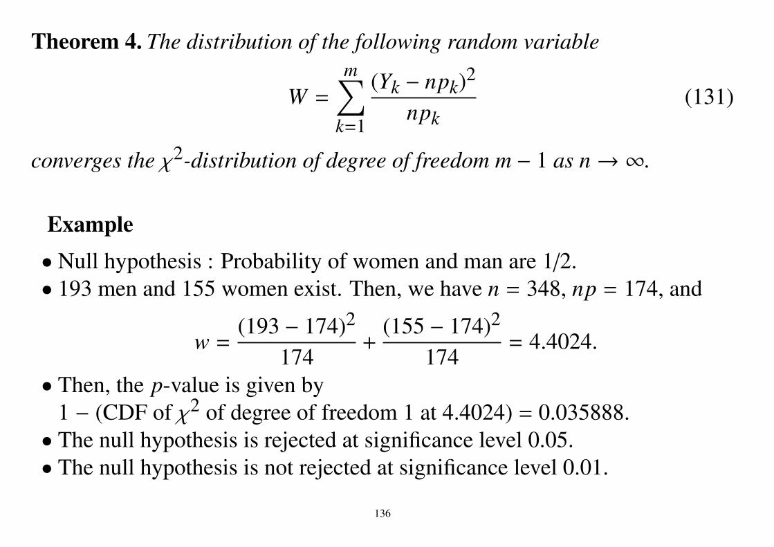
Theorem 4. The distribution of the following random variable
W =m∑
k=1
(Yk − npk)2
npk(131)
converges the χ2-distribution of degree of freedom m − 1 as n→ ∞.
Example• Null hypothesis : Probability of women and man are 1/2.• 193 men and 155 women exist. Then, we have n = 348, np = 174, and
w =(193 − 174)2
174+
(155 − 174)2
174= 4.4024.
• Then, the p-value is given by1 − (CDF of χ2 of degree of freedom 1 at 4.4024) = 0.035888.• The null hypothesis is rejected at significance level 0.05.• The null hypothesis is not rejected at significance level 0.01.
136

(Proof of Theorem)From Laplace’s theorem, Yk converges a normal distribution of which mean
and variance are npk and npk(1 − pk) as n→ ∞. We define random variablesZk by
Zk =Yk − npk√
npk.
It is clear that Zk converges a a normal distribution of which mean and vari-ance are 0 and 1 − pk. We calculate the covariance between Zk and Zl (k , l).
E[ZkZl] = E[Yk − npk√
npk
Yl − npl√npl
]=
1n√
pkplE
[YkYl − npkYl − nplYk + npknpl
]=
1n√
pkpl
(E[YkYl] − npknpl − nplnpk + npknpl
)=
1n√
pkpl
(E[YkYl] − n2pkpl
)137

Since δXi,kδXi,l = 0 (k , l), we have
E[YkYl] = E
n∑
i=1δXi,k
n∑
j=1δX j,l
= n∑
i=1E
[δXi,kδXi,l
]+
n∑i=1
∑j,i
E[δXi,kδX j,l
]= n(n − 1)E
[δX1,kδX2,l
]= n(n − 1)pkpl
Then, we have
E[ZkZl] =1
n√
pkpl
[n(n − 1)pkpl − n2pkpl
]= −√
pkp j.
We can say (Z1 Z2 . . . Zm)T converges to an m-dimensional random variableof a multivariate normal distribution of which variance and covariance aregiven by 1 − pk and −√pkp j, respectively.
Let G = (G1 G2 . . . Gm)T be an m-dimensional random variable of a mul-tivariate standard normal distribution (their variance and covariance are 1 and
138

0, respectively). We define random variables Hk as
Hk = Gk −√
pk
m∑a=1
√paGa.
It is clear that the distribution of H is a multivariate standard normal distribu-tion of which variance and covariance are respectively given by
E[H2k ] = E[G2
k] − 2√
pk
m∑a=1
√paE[GkGa] +
√p2
k
m∑a=1
m∑b=1
√papbE[GaGb]
= E[G2k] − 2
√pk
m∑a=1
√pa δk,a + pk
m∑a=1
m∑b=1
√papb δa,b
= 1 − 2pk + pk
m∑a=1
pa
= 1 − pk,
139
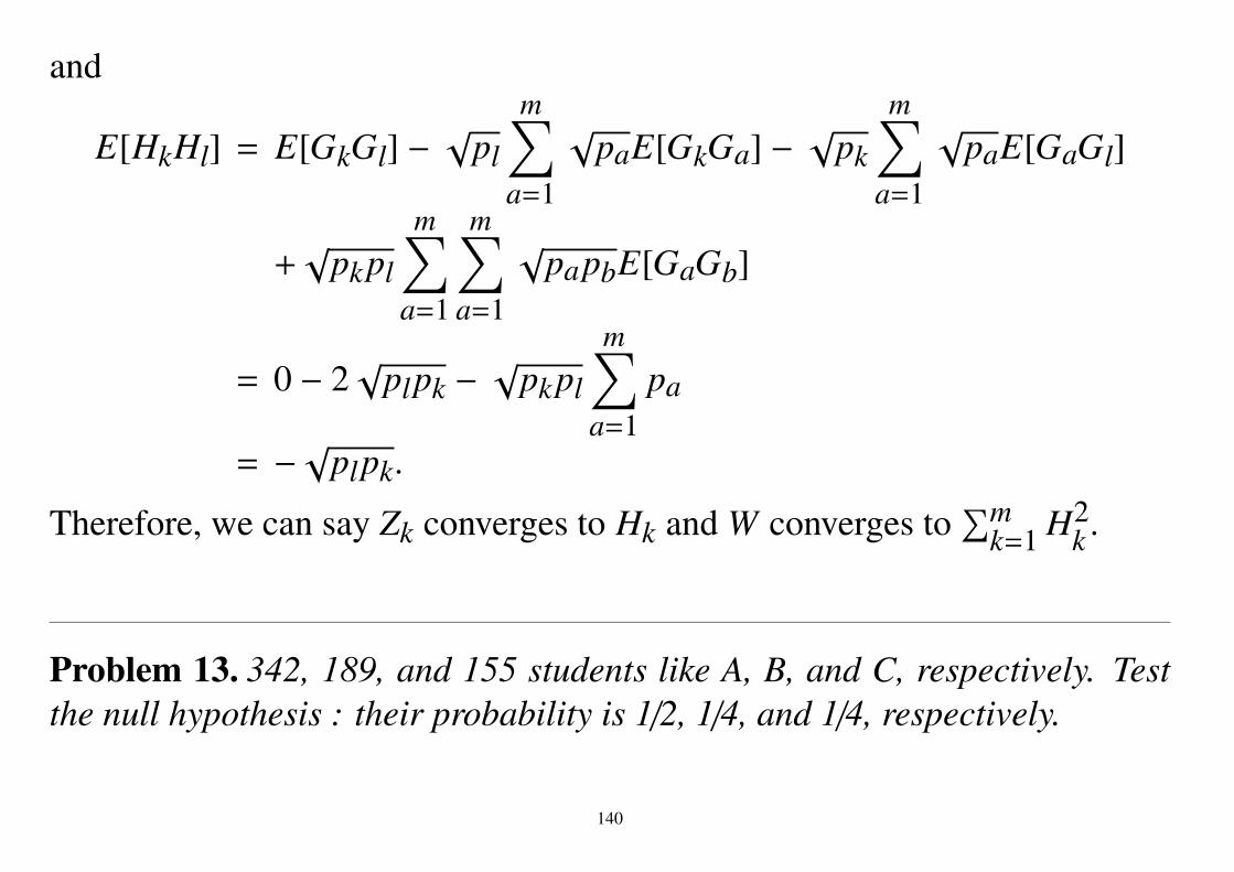
and
E[HkHl] = E[GkGl] −√
pl
m∑a=1
√paE[GkGa] − √pk
m∑a=1
√paE[GaGl]
+√
pkpl
m∑a=1
m∑a=1
√papbE[GaGb]
= 0 − 2√
plpk −√
pkpl
m∑a=1
pa
= −√plpk.
Therefore, we can say Zk converges to Hk and W converges to∑m
k=1 H2k .
Problem 13. 342, 189, and 155 students like A, B, and C, respectively. Testthe null hypothesis : their probability is 1/2, 1/4, and 1/4, respectively.
140

We havem∑
k=1H2
k =m∑
k=1
Gk −√
pk
m∑a=1
√paGa
2
=
m∑k=1
G2k − 2
m∑k=1
Gk√
pk
m∑a=1
√paGa +
m∑k=1
pk
m∑a=1
√paGa
2
=
m∑k=1
G2k −
m∑a=1
√paGa
2
.
Furthermore, we have
E
m∑a=1
√paGa
2 =
m∑a=1
m∑b=1
√pa√
pbE[GaGb] =m∑
a=1pa = 1
Then, Cochran’s theorem yields that the distribution of∑m
k=1 H2k is the χ2-
distribution of degree of freedom m − 1. QED.141

5.6.7 F-test• Two sample sets : extracted independently from two normal distributions• Null hypothesis : variances of two sets of samples are equal• Alternative hypothesis : variances of two sets of samples are not equal• α : significance level• n1 : number of samples in set 1• n2 : number of samples in set 2• σ1
2 : estimated variance of set 1• σ2
2 : estimated variance of set 2•We assume the case that σ1
2 > σ22.
• f = σ12/σ2
2 (Its distribution is F(n1 − 1, n2 − 1))
We define fα as ∫ ∞fα
pF(x)dx = α.
If f > fα, the null hypothesis is rejected at level of significance (significancelevel) α.
142

5.6.8 t-test• Two sample sets : extracted independently from two normal distributions
of which variances are the same.• Null hypothesis : averages of two sets of samples are equal• Alternative hypothesis : averages of two sets of samples are not equal
(One-side test : µ1 − µ2 > 0. Two-side test : µ1 − µ2 , 0.)• α : significance level• n1 : number of samples in set 1• n2 : number of samples in set 2• µ1 : estimated average of set 1• µ2 : estimated average of set 2• σ1
2 : estimated variance of set 1• σ2
2 : estimated variance of set 2• A random variable (t-distribution of n1 + n2 − 2 degree freedom) :
t =µ1 − µ2
σ√
1n1+ 1
n2
143

where
σ2 =(n1 − 1)σ1
2 + (n2 − 1)σ22
n1 + n2 − 2We define tα as ∫ ∞
tαpT (x)dx = α.
If t > tα (one-side test) or ˆ|t| > tα/2 (two-side test), the null hypothesis isrejected at level of significance (significance level) α.
If the variances of the two normal distributions are different, the following tobeys approximately t-distribution
t =µ1 − µ2√σ1
2
n1+σ2
2
n2
144

5.6.9 Test using p-valueχ2-distribution ∫ ∞
χpχ2
1(x)dx
F-distribution ∫ ∞f
pF(x)dx
t-distribution ∫ ∞t
pT (x)dx
If the p-value is smaller than 0.05 or 0.01 the null hypothesis is rejected.
145

6 Estimation6.1 Point estimation• Assume that the probability depends on a parameter (Bosuu in Japanese).• Statistical estimation : estimate the parameter according to observed data.• Let consider the probability p of the case that the front of a coin appears is
a parameter.• Assume that we toss a coin n times and its front appears X times (X is a
random variable).• It is natural to estimate p by
p1 =Xn. (132)
• p1 is also a random variable because X is a random variable.• Estimator means a random variable or a method for estimation.• Estimate means a estimated value.
146

6.2 Bias• Bias : the difference between the mean of an estimator and true value.
E[ p] − p.
• Unbiased estimator : an estimator of which bias is zero (E[p] = p).• Biased estimator : an estimator of which bias is not zero (E[p] , p).• Estimator (132) is an unbiased estimator.
E[ p1] = E[Xn
]=
npn= p.
• Consider an estimatorp2 =
X + 1n + 2
. (133)
It’s mean is given by
E[ p2] = E[X + 1n + 2
]=
np + 1n + 2
.
If p , 1/2, p2 is a biased estimator (E[ p2] , p).
147

6.3 Variance of estimator• Variance of an estimator
V(p) = E[(p − E[ p])2]
• For estimators, small variance is better than large variance.• Example:
V( p1) =1n2V(X) =
1n
p(1 − p)
V( p2) =1
(n + 2)2V(X) =n
(n + 2)2 p(1 − p)
The variance of p2 is smaller than p1.(However, p2 is a biased estimator.)
148

6.4 Mean square error•Mean square error of an estimator is defined by
mse( p) = E[(p − p)2]
•We have
mse( p) = E[( p − p)2]= E[( p − E[ p] + E[p] − p)2]= (E[ p] − p)2 + V( p) (134)
• The meaning of this equation is given by
(mean square error) = (bias)2 + variance.
• Bias variance trade off
Problem 14. Show (134).
149

• Example:
mse(p1) =1n
p(1 − p)
mse(p2) =(np + 1n + 2
− p)2+
n(n + 2)2 p(1 − p)
=−(n − 4)p2 + (n − 4)p + 1
(n + 2)2
When n = 5, p = 0.4, we have mse( p1) = 0.0480 and mse( p2) = 0.0253.In this case, mse of p2 is smaller than that of p1.
150

6.5 Interval estimation• Estimate an interval which includes the parameter.• For the previous example, estimate the lower bound u(X) and the upper
bound v(X) of p from an observed data X.
u(X) ≤ p ≤ v(X) (135)
• Confidence coefficient 1 − α.
P(u(X) ≤ p ≤ v(X)) ≥ 1 − α.under the assumtion p = p. More precisely,
P(ω | u(X(ω)) ≤ p ≤ v(X(ω))) ≥ 1 − α.• In many cases, we let α = 0.05. (Confidence coefficient is 0.95).• Condition (135) is rewritten as
c(p) ≤ X ≤ d(p).
c(p) and d(p) are the inverse functions of v(X) and u(X), respectively.
151

• Therefor, we have
P(c(p) ≤ X ≤ d(p)) ≥ 1 − α. (136)
152

• This formula can be written as
P(X ≤ c(p) or X ≥ d(p)) ≤ α. (137)
• This formula is the same as test. Then, we can use the boundary of a criticalregion to decide c(p) and d(p).• From c(p) and d(p), we can obtain an interval [u(X), v(X)] for p of which
confidence coefficient is 1 − α.• Example: Toss a coin n times. (n is large.) Its front appears X times.• The distribution is approximated by a normal distribution of which average
and variance are np and np(1 − p).• According to two-side test of a normal distribution, the interval is given by
|X − np| ≤ xα/2√
np(1 − p).
• It can be written by
np − xα/2√
np(1 − p) ≤ X ≤ np + xα/2√
np(1 − p).
• By solving above inequality with respect to p, we have the confidence
153

interval.
2nX + nx2α/2 −
√−4nX2x2
α/2 + 4n2Xx2α/2 + n2x4
α/2
2(n2 + nx2α/2)
≤ p ≤2nX + nx2
α/2 +√−4nX2x2
α/2 + 4n2Xx2α/2 + n2x4
α/2
2(n2 + nx2α/2)
• Let p0 be any probability in the confidence interval. We can say the hy-pothesis p = p0 is not rejected at significance level 5%.• Note that it does not mean the probability that p is included in the confi-
dence interval is 1 − α. (The probability is for X.)• Example: n = 100 and X = 40. Let α = 0.05 (xα/2 = 1.96). Confidence
interval of confidence coefficient 0.95 is given by
0.310 ≤ p ≤ 0.498
• Region estimation : for the case that the number of parameters are not one.
154

6.6 Theory of estimationDefinition:
• X : a observed vector : n-dimensional stochastic variable.x : a realized value of X.
• p(x; θ) : the p.d.f. with K-dimensional vector θ (parameters).• Θ : the parameter space (⊂ RK).• Eθ, Vθ : the expectation and the variance of the distribution with p(x; θ)• θ(X) : an estimator for θ (a random variable)• unbiased estimator :
Eθ[θ(X)] = θ.
• uniformly minimum variance unbiased estimator (UMVUE) : θ∗(X) is anunbiased estimator and for any unbiased estimator θ(X) we have
V(θ∗(X)) ≤ V(θ(X)).
155

6.6.1 Cramer-Rao lower boundTheorem 5. 1. Θ is an open set of RK.
2. A = x| p(x; θ) = 0) does not depend of θ.
3. ∀x ∈ A and ∀θ ∈ Θ, there exist ∂∂θi
log p(x; θ) (i = 1, 2, . . . ,K) and they arefinite.
4. The differentials and the integrates are commutative.
5. We define a (K,K)-matrix I (Fisher’s information matrix) as
(I)i j = Eθ
[(∂
∂θilog p(X; θ)
) (∂
∂θ jlog p(X; θ)
)].
6. For a sample X, we define a random variable T as
T =
t1(X)...
tr(X)
.156

We assume that T is an unbiased estimator of
g(θ) =
g1(θ)...
gr(θ)
.7. A matrix D(θ) is defined as
(D(θ))i j =∂
∂θ jgi(θ).
Then we haveVθ(T) − D(θ)(I(θ))−1 D(θ)T ≥ O. (138)
Remark. If we estimate θ itself, gi(θ) = θi.Since D(θ) is a unit matrix, the we have
V(θ) − (I(θ))−1 ≥ 0.
157

(Proof of 1-dimensional case.)We have
Eθ
[∂
∂θlog p(X; θ)
]=
∫1
p(x; θ)∂p(x; θ)∂θ
p(x; θ)dx
=∂
∂θ
∫p(x; θ)dx =
∂
∂θ1 = 0,
and
Eθ
[(T − Eθ[T ])
∂
∂θlog p(X; θ)
]= Eθ
[(T − g(θ))
∂
∂θlog p(X; θ)
]=
∫t(x)
(∂
∂θlog p(x; θ)
)p(x; θ)dx − g(θ)Eθ
[∂
∂θlog p(X; θ)
]=
∂
∂θ
∫t(x)p(x; θ)dx =
∂
∂θEθ[T ] =
∂
∂θg(θ).
158
Then, (∂
∂θg(θ)
)2=
(Eθ
[(T − Eθ[T ])
(∂
∂θlog p(X; θ)
)])2
≤ Eθ[(T − Eθ[T ])2
]Eθ
( ∂∂θ log p(X; θ))2
≤ Vθ(T )I(θ).
It follows that
Vθ(T ) ≥(∂
∂θg(θ)
)I(θ)−1
(∂
∂θg(θ)
). (139)
QED.
• Efficient estimator : an unbiased estimator of which variance achieves theCramer-Rao lower bound.• Every efficient estimator is a UMVUE.
159

6.6.2 Maximum likelihood estimator (MLE)• p(x ; θ) : a probability distribution or a p.d.f. with a parameter θ.• Likelihood function : L(θ) = p(x ; θ).
We reconsider θ is a variable and x is a parameter.• log likelihood function : log L(θ).•Maximum likelihood estimator (MLE) is given by
θ = argmaxθ
L(θ) = argmaxθ
log L(θ)
• Example : estimate the mean and variance of a normal distribution byMLE.– X1, X2, . . . , Xn : i.i.d. (independent and identically distributed) random
variable of a normal distribution.x1, x2, . . . , xn : their realized values.
– Likelihood function L(µ, σ) is given by
L(µ, σ) =nΠ
i=1
1√
2πσe−(xi−µ)2
2σ2 .
160

– Its log likelihood is given by
log L(µ, σ) = − 12σ2
n∑i=1
(xi − µ)2 − n2
log 2π − n logσ
– By letting derivatives be zero, we have equations for MLE.∂
∂µlog L(µ, σ) = 0,
∂
∂σlog L(µ, σ) = 0.
– MLE is given by
µ =1n
n∑i=1
Xi (140)
σ2 =1n
n∑i=1
(Xi − µ)2 (141)
Problem 15. Prove eqs.(140) and (141).161

7 Statistic7.1 Sufficient Statistic• X1, X2, . . . , Xn : observed data (random variables).
x1, x2, . . . , xn : their realized values.• Let t be a function of n variables X1, X2, . . . , Xn.• Statistic : a random variable T defined by
T = t(X1, X2, . . . , Xn)
• θ : a parameter of a distribution.• Assume that a conditional probability or p.d.f.
p(x1, x2, . . . , xn|T = t; θ)
does not depend on θ for any t. ⇒ T is called sufficient statistic.• The condition can be written as
p(x1, x2, . . . , xn; θ) = p(x1, x2, . . . , xn|T = t)p(t; θ).
• It is enough to know T to estimate θ.
162

• Example: Estimate the mean of a normal distribution by its samples.T = X1 + X2 + · · · + Xn
is a sufficient statistic, where X1, X2, . . . , Xn are iid. random variables.(iid. : independent and identically distributed)• Consider its two dimensional case and let
T =1√
2(X1 + X2), U =
1√
2(X1 − X2),
and t and u be realized value of T and U, respectively.• Then, we have (We assume σ2 = 1)
p(x1, x2; µ) = p(x1; µ)p(x2; µ)
=1√
2πe−(x1−µ)2/2 1
√2π
e−(x2−µ)2/2
=1
2πe−
((x1−x2)/
√2)2/2−
((x1+x2)/
√2−√
2µ)2/2.
=1√
2πe−u2/2 1
√2π
e−(t−√
2µ)2/2.
163

andp(x1, x2|T = t; µ) = p(t, u|T = t; µ) =
1√
2πe−u2/2.
It does not depend on µ.• T1,T2, . . . Tm are sufficient statistics with respect to θ:
p(x1, x2, . . . , xn; θ)= p(x1, x2, . . . , xn|T1 = t1,T2 = t2, . . . , Tm = tm) p(t1, t2, . . . , tm; θ).
• Rao-Blackwell’s Theorem– T is a sufficient statistic of a parameter θ.– θ is an unbiased estimator of θ. (θ = θ(X1, X2, . . . , Xn))– We define a new estimator as
θ∗ = E[θ|T ].
– Then θ∗ is also an unbiased estimator of θ and we have
V(θ∗) ≤ V(θ)
(A better estimator can be obtained.)
164

8 Regression8.1 Method of least square• Data : (c1, x2), (c1, x2), . . . , (cn, xn).• For example ci is income, xi is consumption of person i.•We may assume that its relation can be expressed by the first order poly-
nomial.xi = α + βci.
• It will not hold strictly. Let ui is error from the relation.
ui = xi − (α + βci).
•We often minimize their squared sum of uis.
Q =∑
iu2
i =∑
i(xi − α − βci)
2.
•We haveQ = nα2 − 2α
∑i
(xi − βci) +∑
i(xi − βci)
2. (142)
165

•With respect to α, eq.(142) is minimized when
α ≡ 1n
∑i
(xi − βci) = x − βc, (143)
wherec =
1n
∑i
ci, x =1n
∑i
xi.
•We substitute α into α in eq.(142).
Q = β2∑
i(ci − c)2 − 2β
∑i
(ci − c)(xi − x) +∑
i(xi − x)2 (144)
Problem 16. Prove eq.(144).
• β is given by
β =
∑i(ci − c)(xi − x)∑
i(ci − c)2 . (145)
⇒ Linear regression.(Method of least square).
166

• Letxi = α + βci.
Then, we haveQ =
∑i
(xi − xi)2.
• If Q is small comparing to∑
i(xi− x)2, the assumption seems to be correct.•We define r2 as
r2 = 1 − Q∑i(xi − x)2.
If r2 is near to 1, the assumption seems to be correct.• By substituting β into β in eq.(144), we have
Q =∑
i(xi − x)2 −
∑i(ci − c)(xi − x)
2∑i(ci − c)2 .
and
r2 =
∑i(ci − c)(xi − x)
2∑i(xi − xi)2 ∑
i(ci − c)2.
167

8.2 Linear model• Xi (i = 1, 2, . . . , n) : random variables of normal distribution of which
variances are σ2. (The distribution of Xi are different).• θ j ( j = 1, 2, . . . ,m) : parameter to decide the mean. (m < n).
E[Xi] =n∑
j=1Ci jθ j
where Ci j is the (i, j)-element of a given matrix C.•We define random variables as
Z =n∑
i=1X2
i ,
Y j =n∑
i=1Ci jXi.
• (Z,Y1, . . . , Ym) are the sufficient statistics of σ, θ1, θ2, . . . , θm.
168

•We have
E[Y j] = E
n∑i=1
Ci jXi
= n∑i=1
Ci jE[Xi] =n∑
i=1
n∑k=1
Ci jCikθk
• θ j : estimator of θ j satisfies
Y j =n∑
k=1
n∑i=1
Ci jCikθk (146)
•We define
X =
X1X2...
Xn
, Y =
Y1Y2...
Ym
, Θ =
θ1θ2...θm
, Θ =
θ1θ2...
θm
.• Eq.(146) yields the normal equation:
CT CΘ = DΘ = Y. (147)
where D = CT C.169

• Estimator of Θ is given by
Θ = D−1Y. (148)
• Θ is an unbiased estimator. Since E[X] = CΘ, we have
E[Θ] = (CT C)−1E[Y] = D−1CT E[X] = D−1 DΘ = Θ.
• The variance covariance matrix of Y, V(Y), is given by
V(Y) = E[(Y − E[Y])(Y − E[Y])T ] = CT E[(X − E[X])(X − E[X])T ]C= CT (σ2I)C = σ2 D.
• The variance covariance matrix of Θ (used in regression) is given by
V(Θ) = E[(Θ − E[Θ])(Θ − E[Θ])T ]= D−1E[(Y − E[Y])(Y − E[Y])T ]D−1 = D−1(σ2 D)D−1 = σ2 D−1
•We define random variables as
Ui = Xi − E[Xi]Vi = θi − θi
170

•We also define
U =
U1U2...
Un
(= X − E[X]), V =
V1V2...
Vm
(= Θ −Θ).
• E[U] = 0, E[V] = 0 andV = D−1CT U.
• Since E[X] = CΘ, the residue Q is given by
Q =n∑
i=1
Xi −m∑
j=1Ci jθ j
2
=∑
i
Ui −m∑
j=1Ci jV j
2
=
n∑i=1
U2i −
m∑j=1
m∑k=1
D jkV jVk
• V(V)(= V(Θ)) is given by σ2 D−1. Therefore, the distribution of1σ2
∑mj=1
∑mk=1 D jkV jVk is a χ2-distribution of m degree of freedom.
171

• Since Vi are linear combination of Ui,Qσ2 =
1σ2
∑i
U2i −
1σ2
∑j
∑k
D jkV jVk
is the χ2-distribution of (n − m) degree of freedom.• Since Y = CT X and Θ = D−1CT X, we also have
Q = ∥X − CΘ∥2 =n∑
i=1X2
i −m∑
j=1Y jθ j
• The estimator of σ2 is given by
σ2 =1
n − m
n∑i=1
X2i −
m∑j=1
Y jθ j
172

8.3 Theory of regression• Linear regression equation :
E(X) = α + βc.
• c : explaining variable• X : dependent variable• α, β : regression coefficient• The problem is to estimate regression coefficients.• Let Xi is samples at ci.
We consider the average and variance of Xi are given by α + βci and σ2,respectively.• ci is not a random variable.• Linear regression equation can be rewritten by
X = α + βc + U.
• U : error. The distribution of U is assumed to be identical for all samplepoints and its average is zero.
173

• Use the linear model. We consider θ1 = α, θ2 = β,
C =
1 c11 c2... ...1 cn
.•We have
Y1 =n∑
i=1Ci1Xi =
n∑i=1
Xi,
Y2 =n∑
i=1Ci2Xi =
n∑i=1
ciXi,
D =(
n ncnc
∑ni=1 c2
i
).
D−1 =1
n∑n
i=1(ci − c)2
( 1n∑n
i=1 c2i −c
−c 1
).
174

• The estimators of α and β are given by(α
β
)= D−1
( ∑ni=1 Xi,∑n
i=1 ciXi
)(149)
Eq.(149) is equivalent to (143) and (145).• The estimator of σ2 (variance of Xi) is given by
σ2 =1
n − 2Q =
1n − 2
n∑i=1
X2i − α
n∑i=1
Xi − βn∑
i=1ciXi
=
1n − 2
∑i
(Xi − X)2 −
∑i(ci − c)(Xi − X)
2∑i(ci − c)2
.• The variance covariance matrix of α and β is given by
V(α, β) =
σ2α Cov(α, β)
Cov(α, β) σ2β
= σ2 D,
where Cov(α, β) = E(α − α)(β − β).175

• Its estimator is given by
V(α, β) =
σ2α
ˆCov(α, β)ˆCov(α, β) σ2
β
= σ2 D.
• Hypothesis : α = α0.
α − α0√σ2α
obeys t-distribution of n − 2 degree of freedom.⇒We can test the hypothesis or calculate its confidence interval.• Hypothesis β = β0 yields
β − β0√σ2β
also obeys t-distribution of n − 2 degree of freedom.
176

9 Statistical learning theory9.1 Framework• z: pattern• Pattern are observed randomly.• F(z): cumulative probability distribution function•When z is a real number, F(z) is defined as a probability of the case that a
pattern Z satisfying Z ≤ z is observed.• The ensemble expectation of g(z) with respect to z is given by
Eg(z) ≡∫
g(z)dF(z). (150)
If F(z) is differentiable, its probability density function (p.d.f) f (x) is givenby
f (z) =dFdz.
(The probability of the case that a pattern in [z, z+dz] is observed is f (z)dz.)
177
•When we use the p.d.f., expectation of g(z) is given as
Eg(z) =∫
g(z) f (z)dz.
(By using not f (z) but F(z), expectation with respect to discrete valuessuch as dice can be expressed.)• Assumption: each pattern has its category.• Assumption: a family of (classification) functions dα(z) (α ∈Λ) that returns
a category for an input pattern z.• Λ is the set of α that is the indicator of classification function.⇔ Each classification function corresponds to an element α in Λ.• Assumption: a risk function is given as follows.
R(z, y) ≡
0 (The category of pattern z is y)1 (else) .
•We define a function Q(α, z) with a classification function dα(z).
Q(α, z) ≡ R(z, dα(z)) =
0 (the result of dα(z) is correct)1 (the result of dα(z) is incorrect) .
178
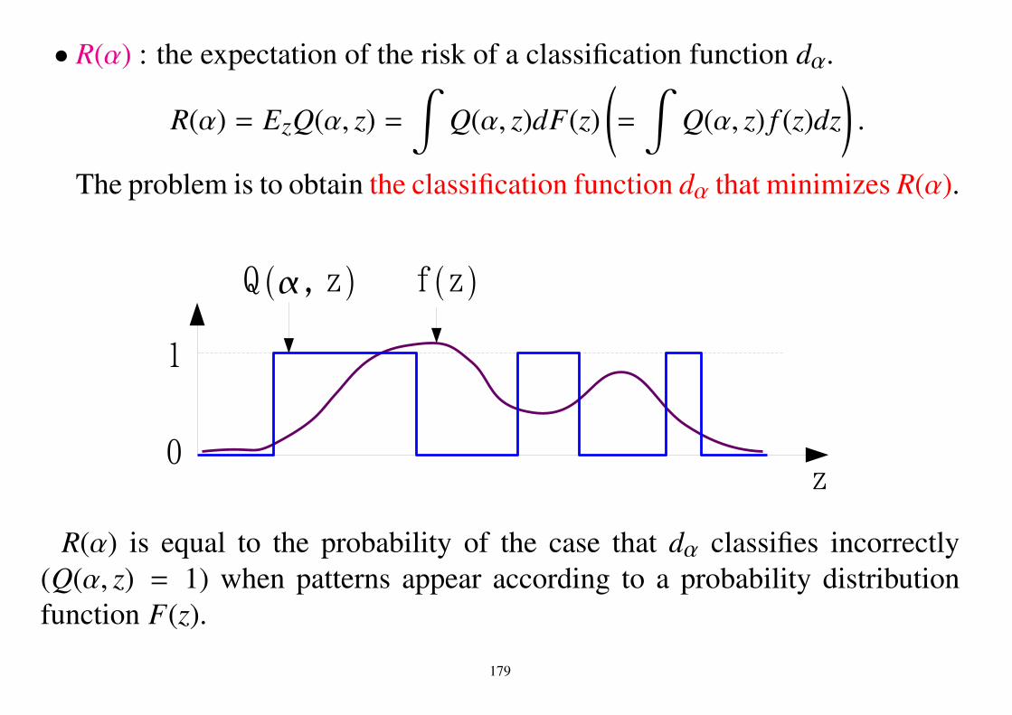
• R(α) : the expectation of the risk of a classification function dα.
R(α) = EzQ(α, z) =∫
Q(α, z)dF(z)(=
∫Q(α, z) f (z)dz
).
The problem is to obtain the classification function dα that minimizes R(α).
R(α) is equal to the probability of the case that dα classifies incorrectly(Q(α, z) = 1) when patterns appear according to a probability distributionfunction F(z).
179

PQ(α, z) = 1 =∫z |Q(α,z)=1
dF(z)(=
∫z |Q(α,z)=1
f (z)dz)
=
∫Q(α, z)dF(z)
= R(α).
180

• For learning, we can use only finite number of patterns.• L : the number of learning patterns.
z1, z2, . . . , zL.
• Assumption: we know the category of each learning patterns.• The risk of a classification function for learning patterns is calculated by
Remp(α) =1L
L∑i=1
Q(α, zi).
We call it the empirical risk.• The difference between two risks is evaluated in statistical learning theory.
R(α) =∫
Q(α, z)dF(z),
Remp(α) =1L
L∑i=1
Q(α, zi).
⇒ Estimate the ensemble expectation from the sample expectation.181

• Application: evaluation of ERM principle
Definition 4. ERM (empirical risk minimization) principleUse dα that minimized Remp(α).
• Learning patterns appear according to a p.d.f. f (z).• Estimate the expectation of Q(α, z) from Q(α, zi) for learning patterns zi.
182

9.2 Expectation and supremum• The expectation of g(z1, z2, . . . , zL) with z1, z2, . . . , zL :
Ez1,z2,...,zLg(z1, z2, . . . , zL)
≡∫ ∫
· · ·∫
g(z1, z2, . . . , zL)dF(z1)dF(z2) · · · dF(zL).
• The supremum of g(z1, z2, . . . , zL) with z1, z2, . . . , zL :
supz1,z2,...,zL
g(z1, z2, . . . , zL).
• For any distribution and any function g, we have
Ez1,z2,...,zLg(z1, z2, . . . , zL) ≤ supz1,z2,...,zL
g(z1, z2, . . . , zL).
9.3 Entropy, annealed entropy, growth function• NΛ(z1, z2, . . . , zL) : the number of different (Q(α, z1),Q(α, z2), . . .Q(α, zL))
when we fix (z1, z2, . . . , zL) and vary α ∈ Λ.• That is the number of different types of risk array of classification functions
for fixed input patterns.183

• Entropy :HΛ(L) = Ez1,z2,...,zL ln NΛ(z1, z2, . . . , zL)
• Annealed entropy :
HΛann(L) = ln Ez1,z2,...,zLNΛ(z1, z2, . . . , zL)
• Growth function :
GΛ(L) = ln maxz1,z2,...,zL
NΛ(z1, z2, . . . , zL)
•We have following relation.
HΛ(L) ≤ HΛann(L) ≤ GΛ(L)
Problem 17. Prove
ln αx1 + (1 − α)x2 ≥ α ln x1 + (1 − α) ln x2
for x1(> 0), x2(> 0), and α (0 ≤ α ≤ 1).
184

Hinto of Problem 17Let f (x) = ln x. It is clear that
d2 f (x)dx2 < 0 (151)
for all x > 0. We define a function as
F(x) = f (x) −
f (x2) − f (x1)x2 − x1
(x − x1) + f (x1).
We haveF(x1) = F(x2) = 0,
F(αx1 + (1 − α)x2) = f (αx1 + (1 − α)x2) − α f (x1) + (1 − α) f (x2),F. (x)dx=
d f (x)dx− f (x2) − f (x1)
x2 − x1,
andd2F(x)
dx2 =d2 f (x)
dx2 . (152)
185

From eqs.(1) and (2), dF(x)dx is monotone decreasing. Then, the number of
extreme points of F(x) (x1 ≤ x ≤2) is one at most. From the intermediatevalue theorem, there exists c (x1 ≤ c ≤ x2) such that
dF(x)dx
∣∣∣∣∣x=c=
d f (x)dx
∣∣∣∣∣x=c− f (x2) − f (x1)
x2 − x1= 0.
Then, you can prove F(x) ≥ 0 (x1 ≤ x ≤2) from the above relations.(End of Hinto)
9.3.1 Basic inequalityThe following theorem is one of the most important theorems for statisticallearning theory.
186

Theorem 6. We have following relation. (Basic inequality)
P
supα∈Λ|R(α) − Remp(α)| > ε
< 4 exp
HΛann(2L)
L−
(ε − 1
L
)2 L
.• The left hand side is the probability that learning patterns (z1, z2, . . . , zL)
appears, with which the maximum absolute difference between the ensem-ble risk and the empirical risk among all α ∈ Λ is larger than ε.• Since HΛann(2L) < GΛ(2L), the above inequality holds even if we replace
HΛann(2L) to GΛ(2L).• Let η be the right hand of the basic inequality.
η = 4 exp
HΛann(2L)
L−
(ε − 1
L
)2 L
.Solve it with respect to ε, and we have
ε =
√HΛann(2L) − ln(η/4)
L+
1L.
187

Corollary 1. We have the following relation with probability 1 − η.
|R(α) − Remp(α)| ≤
√HΛann(2L) − ln(η/4)
L≤
√GΛ(2L) − ln(η/4)
L.
DefinitionsZ2L = (z1, . . . , zL, zL+1, . . . , z2L)
Z1 = (z1, . . . , zL), Z2 = (zL+1, . . . , z2L)
ν(α,Z1) =1L
L∑i=1
Q(zi, α), ν(α, Z2) =1L
2L∑i=L+1
Q(zi, α)
ρ(α, Z2L) = |ν(α, Z1) − ν(α, Z2)|π(α,Z1) =
∣∣∣∣∣∫ Q(α, z)dF − ν(α,Z1)∣∣∣∣∣ = ∣∣∣R(α) − Remp(α))
∣∣∣Lemma 11. (Basic Lemma)
P
supα∈Λ
π(α,Z1) > ε< 2P
supα∈Λ
ρ(α, Z2L) > ε − 1L
188

(Proof.)First, we fix α∗ and consider the case that samples satisfy R(α∗) > ν(α∗,Z1).
We denote the probability of the case C under that condition by P1C. Thatis, P1C ≡ PC |R(α∗) > ν(α∗,Z1). Then, for any α∗ ∈ Λ, we have thefollowing equation
P1
supα∈Λ
ρ(α, Z2L) > ε − 1L
≥ P1
(supα∈Λ
ρ(α, Z2L) > ε − 1L
)∧ (π(α∗,Z1) > ε
)≥ P1
(ρ(α∗,Z2L) > ε − 1
L
)∧ (π(α∗,Z1) > ε
)= P1
(∣∣∣ν(α∗,Z1) − ν(α∗,Z2)∣∣∣ > ε − 1
L
)∧
(∣∣∣R(α∗) − ν(α∗,Z1)∣∣∣ > ε)
= P1
(∣∣∣ν(α∗,Z1) − ν(α∗,Z2)∣∣∣ > ε − 1
L
)∧ (
R(α∗) − ν(α∗,Z1) > ε)
(153)189

The following logic relation is clear.(ν(α∗,Z2) > R(α∗) − 1
L
)∧ (
R(α∗) − ν(α∗,Z1) > ε)
⇒(−ν(α∗,Z1) + ν(α∗,Z2) > ε − 1
L
)∧ (
R(α∗) − ν(α∗,Z1) > ε)
⇒(∣∣∣ν(α∗,Z1) − ν(α∗,Z2)
∣∣∣ > ε − 1L
)∧ (
R(α∗) − ν(α∗,Z1) > ε).
In the relation, it is clear that the probability of the case that the last conditionis true is not less than that of the first condition.
P1
(∣∣∣ν(α∗,Z1) − ν(α∗,Z2)∣∣∣ > ε − 1
L
)∧ (
R(α∗) − ν(α∗,Z1) > ε)
≥ P1
(ν(α∗,Z2) > R(α∗) − 1
L
)∧ (π(α∗,Z1) > ε
)
190

Since Z1 and Z2 are sampled independently.
P1
(ν(α∗,Z2) > R(α∗) − 1
L
)∧ (π(α∗,Z1) > ε
)= P1
(ν(α∗,Z2) > R(α∗) − 1
L
)· P1
(π(α∗,Z1) > ε
)• For a sample z, the probability of the case that Q(α∗, z) = 1 is R(α∗).• Consider a coin of which probability of the front side for a tossing is R(α∗).•When we toss it L times and it shows the front Lν(α∗,Z2) times, the prob-
ability of the case that Lν(α∗,Z2) is greater than LR(α∗) − 1 is greater than1/2. (This is a property of binomial distribution.)• The first probability in the right hand side of the above inequality is the
same as the above probability and greater than 1/2.
From those relation we have
P1
supα∈Λ
ρ(α, Z2L) > ε − 1L
>
12
P1(π(α∗,Z1) > ε
).
191

Next, we consider the case R(α∗) ≤ ν(α∗,Z1). We denote the probabilityunder the condition by P2. Then, considering the case ν(α∗,Z2) < R(α∗) + 1
L,we can similarly prove
P2
supα∈Λ
ρ(α, Z2L) > ε − 1L
>
12
P2(π(α∗,Z1) > ε
).
When we recall the calculation of a marginal distribution,PR(α∗) > ν(α∗,Z1) + PR(α∗) ≤ ν(α∗,Z1) = 1 yields
P1C · PR(α∗) > ν(α∗,Z1) + P2C · PR(α∗) ≤ ν(α∗,Z1) = PC.for any case C. It completes the proof. Q.E.D.(Proof of basic inequality)• Denote the operation of permutation of 2L samples by Ti (i = 1, 2, . . . , (2L)!).• Since they are sampled independently, the probability is not changed by
the permutation:
P
supα∈Λ
ρ(α, Z2L) > ε − 1L
= P
supα∈Λ
ρ(α, TiZ2L) > ε − 1
L
192
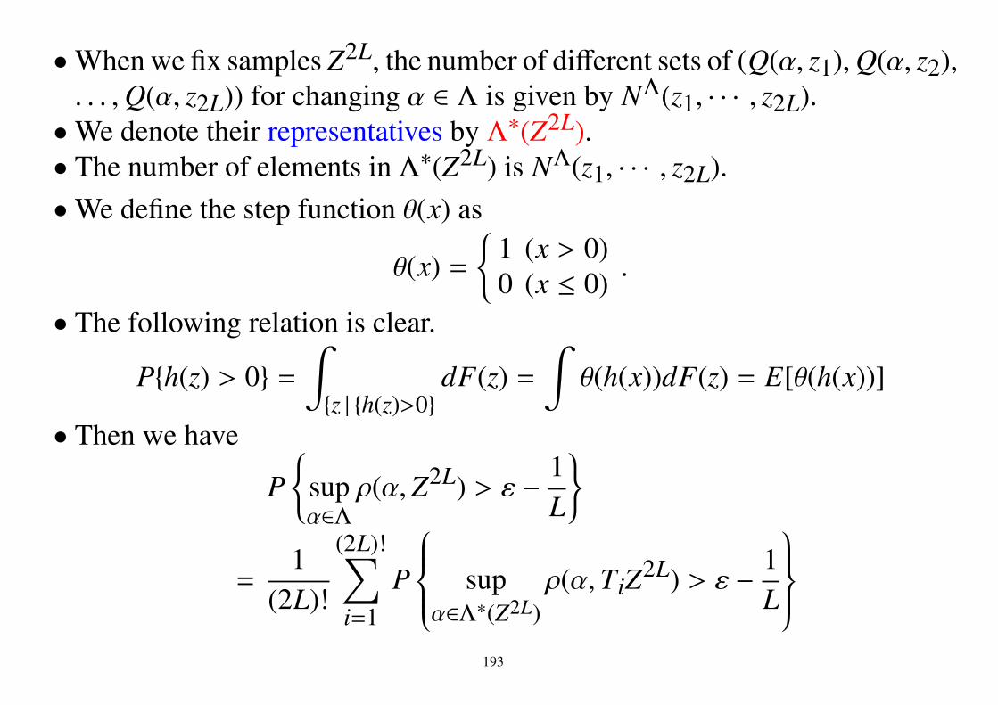
•When we fix samples Z2L, the number of different sets of (Q(α, z1),Q(α, z2),. . . ,Q(α, z2L)) for changing α ∈ Λ is given by NΛ(z1, · · · , z2L).•We denote their representatives by Λ∗(Z2L).• The number of elements in Λ∗(Z2L) is NΛ(z1, · · · , z2L).•We define the step function θ(x) as
θ(x) =
1 (x > 0)0 (x ≤ 0) .
• The following relation is clear.
Ph(z) > 0 =∫z | h(z)>0
dF(z) =∫
θ(h(x))dF(z) = E[θ(h(x))]
• Then we have
P
supα∈Λ
ρ(α,Z2L) > ε − 1L
=
1(2L)!
(2L)!∑i=1
P
supα∈Λ∗(Z2L)
ρ(α, TiZ2L) > ε − 1
L
193

=1
(2L)!
(2L)!∑i=1
P
supα∈Λ∗(Z2L)
ρ(α,TiZ2L) − ε + 1
L> 0
=
1(2L)!
(2L)!∑i=1
E
θ supα∈Λ∗(Z2L)
ρ(α, TiZ2L) − ε + 1
L
≤ 1(2L)!
(2L)!∑i=1
E
∑α∈Λ∗(Z2L)
θ
(ρ(α, TiZ
2L) − ε + 1L
)= E
∑α∈Λ∗(Z2L)
1(2L)!
(2L)!∑i=1
θ
(ρ(α, TiZ
2L) − ε + 1L
) .• Assume that among Q(α, z1),Q(α, z2), . . . ,Q(α, z2L), m of them are 1 and
the others (2L − m of them) are 0.
194

• From the definition ρ(α, Z2L) can be written as
ρ(α,Z2L) =
∣∣∣∣∣∣∣∣1LL∑
i=1Q(zi, α) − 1
L
2L∑i=L+1
Q(zi, α)
∣∣∣∣∣∣∣∣ . (154)
• Assume that among the first and the second terms in eq.(154) k and m − kQ(zi, α) are 1, respectively.• Then, we have
ρ(α, Z2L) =∣∣∣∣∣kL − m − k
L
∣∣∣∣∣ .• The learning patters are reordered by Ti.
θ
(ρ(α, TiZ
2L) − ε + 1L
)is 1 if and only if k that is the number of Q(zi, α) equals to 1 in the firstsum in ρ(α, TiZ2L) satisfies∣∣∣∣∣kL − m − k
L
∣∣∣∣∣ > ε − 1L.
195

• nCk denotes the number of combinations taking k from n.
A set of integers K is defined by
K =
k∣∣∣∣∣ ∣∣∣∣∣kL − m − k
L
∣∣∣∣∣ > ε − 1L
.
•We have
1(2L)!
(2L)!∑i=1
θ
(ρ(α,TiZ
2L) − ε + 1L
)=
∑k∈K
mCk 2L−mCL−k
2LCL. (155)
• Consider m red and 2L − m blue balls and we splits them into two bags.Each bag includes L balls. The left hand side of eq.(155) equals to thenumber of cases when the first bag has k red ball for all k ∈ K divided by(2L)!.•We can prove the following equation holds for any m.∑
k∈K
mCk 2L−mCL−k
2LCL< 2 exp
−(ε − 1
L
)2 .
196

Then, the followings hold and the basic inequality is proven.
P
supα∈Λ|R(α) − Remp(α)| > ε
≤ 2P
supα∈Λ
ρ(α,Z2L) > ε − 1L
≤ 2E
∑α∈Λ∗(Z2L)
1(2L)!
(2L)!∑i=1
θ
(ρ(α, TiZ
2L) − ε + 1L
)< 2E
∑α∈Λ∗(Z2L)
2 exp
−(ε − 1
L
)2
= 4E[NΛ(z1, . . . , z2L)
]exp
−(ε − 1
L
)2
= 4 exp
HΛann(2L)
L−
(ε − 1
L
)2 L
.197

9.4 VC (Vapnik-Chervonenkis) dimension• For a growth function for a set of classifiers
GΛ(L) = ln maxz1,...,zL
NΛ(z1, . . . , zL),
we have the following theorem.
Theorem 7. For any integer L, we have GΛ(L) = L ln 2 or there exists aninteger h (VC dimension) such that
GΛ(L)
= L ln 2 (L ≤ h)≤ ln
(∑hi=0 LCi
)(L > h)
.
•When the number of samples is less than or equal to h, there exists anclassifier that splits all samples correctly for any labeling of samples.
198

Lemma 12. If we have
NΛ(z1, z2, . . . , zL) >m∑
i=0LCi,
there exists a subsequence of samples z∗1, z∗2, . . . , z∗m+1 such that
NΛ(z∗1, z∗2, . . . , z∗m+1) = 2m+1.
Now, we prove Theorem 7. Let
h = argmaxL
(GΛ(L) = L ln 2.
)Let z1, z2, . . . , zh be the set of h elements that achieves the maximum. It isclear that for any L ≤ h we have
GΛ(L) = L ln 2.
with any L elements in z1, z2, . . . , zh because NΛ(z1, z2, . . . , zh) = 2h meansany separation of the set is possible by choosing α ∈ Λ.
199

Suppose that for some L(> h) we have
GΛ(L) > lnh∑
i=0LCi,
then from Lemma 12 there exists h + 1 elements such that
NΛ(z∗1, z∗2, . . . , z∗h+1) = 2h+1.
Then, we haveGΛ(h + 1) = (h + 1) ln 2.
This equality contradicts the choice of h.
200

When VC dimension h is defined for Λ, we have
HΛann(L) ≤ GΛ(L) ≤ ln
h∑i=1
LCi
≤ h(1 + ln
Lh
).
Then we have the following theorem and corollary.(We omit the proof of the last inequailty).
Theorem 8.
P
supα∈Λ|R(α) − Remp(α)| > ε
< 4 exp
h(1 + ln(2L/h))
L−
(ε − 1
L
)2 L
.
201

9.4.1 VC dimension and risk
Corollary 2. With probability 1 − η the following relation holds.
R(α) − Remp(α) ≤√
h(1 + ln(2L/h)) − ln(η/4)L
.
202

9.4.2 Linear classifier and VC dimension
• VC dimension of the set of all linear classifiers in Rn : n + 1
203

9.4.3 Margin and VC dimension
• Assume that the norm of patterns are upper bounded. The larger marginthe fewer VC dimension is.
204

(Lemma 12)If we have
NΛ(z1, z2, . . . , zL) >m∑
i=0LCi,
there exists a subsequence z∗1, z∗2, . . . , z∗m+1 such that
NΛ(z∗1, z∗2, . . . , z∗m+1) = 2m+1.
(Proof of Lemma 12)We define φ(n, L) as
φ(n, L) =n−1∑i=0
LCi.
We define LCi = 0 if i > L.It is clear that
φ(1, L) = LC0 = 1.
205

When L < n we have
φ(n, L) =n−1∑i=0
LCi =L∑
i=0LCi = (1 + 1)L = 2L
The property of the combination
LCi = L−1Ci + L−1Ci−1
yieldsφ(n, L) = φ(n, L − 1) + φ(n − 1, L − 1).
Let n = m+1 and we prove this lemma with respect to n by the mathematicalinduction.
First, let n = 1. If we have
NΛ(z1, . . . , zL) > φ(1, L) = 1,
for at least one z∗ ∈ z1, . . . , zL there exists α0, α1 ∈ Λ such that
Q(z∗, α0) = 0, Q(z∗, α1) = 1.
206

This relation yieldsNΛ(z∗) = 2.
Then, Lemma 12 for n = 1 holds.Next, when n ≤ n0, Lemma 12 holds for any L and any Λ and consider the
case n = n0 + 1.When L < n0 + 1, the assumption of Lemma 12 is written as
NΛ(z1, . . . , zL) > φ(n0 + 1, L) = 2L.
However, since NΛ(z1, . . . , zL) is not larger than 2L, the assumption does nothold and the lemma holds for this case.
Then, we assume that when L ≤ L0, Lemma 12 holds for anyΛ and considerthe case L = L0 + 1. Now, the assumption of Lemma 12
NΛ(z1, . . . , zL0+1) > φ(n0 + 1, L0 + 1)
holds.We consider the following two cases.
207
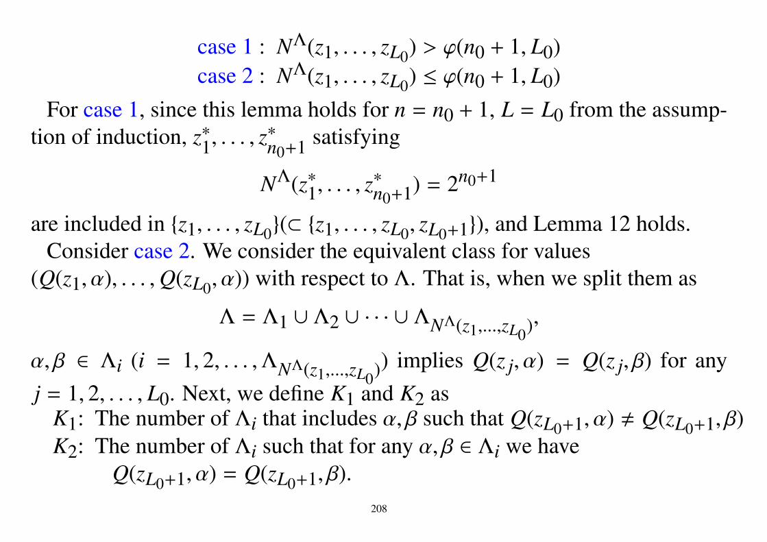
case 1 : NΛ(z1, . . . , zL0) > φ(n0 + 1, L0)case 2 : NΛ(z1, . . . , zL0) ≤ φ(n0 + 1, L0)
For case 1, since this lemma holds for n = n0 + 1, L = L0 from the assump-tion of induction, z∗1, . . . , z
∗n0+1 satisfying
NΛ(z∗1, . . . , z∗n0+1) = 2n0+1
are included in z1, . . . , zL0(⊂ z1, . . . , zL0, zL0+1), and Lemma 12 holds.Consider case 2. We consider the equivalent class for values
(Q(z1, α), . . . ,Q(zL0, α)) with respect to Λ. That is, when we split them as
Λ = Λ1 ∪ Λ2 ∪ · · · ∪ ΛNΛ(z1,...,zL0),
α, β ∈ Λi (i = 1, 2, . . . ,ΛNΛ(z1,...,zL0)) implies Q(z j, α) = Q(z j, β) for anyj = 1, 2, . . . , L0. Next, we define K1 and K2 as
K1: The number of Λi that includes α, β such that Q(zL0+1, α) , Q(zL0+1, β)K2: The number of Λi such that for any α, β ∈ Λi we have
Q(zL0+1, α) = Q(zL0+1, β).208

Then, we have
NΛ(z1, . . . , zL0) = K1 + K2,
NΛ(z1, . . . , zL0, zL0+1) = 2K1 + K2,
andNΛ(z1, . . . , zL0, zL0+1) = K1 + NΛ(z1, . . . , zL0).
Let’s extract an element αi fromΛi that satisfies the condition for K1. LetΛ∗
be the set of all such αi. From the rule of choosingΛi, (Q(z1, α), . . . ,Q(zL0, α))for the element in Λ∗ are different from each other. Then, we have
NΛ∗(z1, . . . , zL0) = K1.
When K1 > φ(n0, L0), since Lemma 12 holds for n = n0, L = L0, andΛ = Λ0, there exists a subsequence z∗1, . . . , z
∗n0 such that
NΛ∗(z∗1, . . . , z
∗n0) = 2n0.
209

Furthermore, the condition of K1 yields
2n0+1 ≥ NΛ(z∗1, . . . , z∗n0, zL0+1) ≥ 2NΛ
∗(z∗1, . . . , z
∗n0) = 2n0+1.
Then, Lemma 12 holds.When K1 ≤ φ(n0, L0), the condition of case 2 yields
NΛ(z1, . . . , zL0, zL0+1) = K1 + NΛ(z1, . . . , zL0)≤ φ(n0, L0) + φ(n0 + 1, L0)= φ(n0 + 1, L0 + 1).
This relation implies that the assumption of Lemma 12 does not hold.This completes the proof. QED.
9.5 References• Vladimir N. Vapnik, “Statistical Learning Theory,” Wiley, New-York, 1998.• K.-R. Muller and S. Mika and G. Ratsch and K. Tsuda and B. Scholkopf,
“An Introduction to Kernel-Based Learning Algorithms,” IEEE Transac-tions on Neural Networks, Vol.12, No.2, pp. 181–201, 2001.
210

10 OptimizationConsider minimizing a function
J : Rn → R.
211

10.1 Gradient methodAssume that J is continuously differentiable. Let
x =
x1...
xn
, a =
a1...
an
.The Taylor expansion at x = a is given as
J(x1, . . . , xn) = J(a1, . . . , an) +∂J∂x1
∣∣∣∣∣∣x=a(x1 − a1) + · · · + ∂J
∂xn
∣∣∣∣∣x=a(xn − an)
+(not less than second order terms).
We define
J1(x1, . . . , xn) = J(a1, . . . , an) +∂J∂x1
∣∣∣∣∣∣x=a(x1 − a1) + · · · + ∂J
∂xn
∣∣∣∣∣x=a(xn − an).
(156)JI expresses the tangential plane of J at x = a.
212

213

Gradient of J:
∇J =
∂J∂x1...∂J∂xn
.JI(x) = J(a) + ⟨∇J|x=a, x − a⟩.
∇J|x=a is perpendicular to the contour-line of J.In Rn+1, the vector (∇J|x=a,−1) is perpendicular to the tangential plane
JI(x).⟨(∇J|x=a,−1), (x − a, J1(x) − J1(a))⟩ = 0
Gradient method: Search the minimum point by using ∇J.
214

10.1.1 Maximum gradient methodIt searches the minimum point in the direction ∇J. For brief ∇J|x=a is de-noted by ∇J[a].
Algorithm1. x1 : an initial point. Let k = 1.
2. Calculate ∇J[xk].
3. If ∥∇J[xk]∥ is enough small, then stop.
4. Search the (local) minimum point in the direction ∇J[xk](linear search), and let xk+1 be the point.
5. k ← k + 1.
6. Go to 2.
If xk+1 is a local minimum, we have
∇J[xk+1] ⊥ ∇J[xk]
215

Calculation of ∇J
• Analytic• Difference:
∇J ≃
J(x1+δ,x2,...,xn)−J(x1−δ,x2,...,xn)
2δ...
J(x1,x2,...,xn+δ)−J(x1,x2,...,xn−δ)2δ
216

Linear search
F(t) = J(a − t∇J[a])In general, the minimum point of F(t) is not the minimum point of J(x).
A simple algorithm for linear search1. Choose initial values t1, t2, and t3 such that t1 < t2 < t3, F(t1) >
F(t2), and F(t3) > F(t2).
2. Fit a quadratic function with t1, t2, and t3. Let t0 be the minimumpoint of the quadratic function fitting the three points.
3. If t0 < t2 and F(t0) < F(t2), then t1 ← t1, t2 ← t0, t3 ← t2.If t0 < t2 and F(t0) > F(t2), then t1 ← t0, t2 ← t2, t3 ← t3.If t0 > t2 and F(t0) < F(t2), then t1 ← t2, t2 ← t0, t3 ← t3.If t0 > t2 and F(t0) < F(t2), then t1 ← t1, t2 ← t2, t3 ← t0.
4. Go to 2.
217

218

10.1.2 Conjugate gradient method for quadratic functionFirst, we consider a quadratic function in Rn. For a symmetric matrix A wedefine
J(x) =12⟨Ax, x⟩ + ⟨b, x⟩ + c =
12
∑i
∑j
Ai jxix j +∑
ibixi + c
A non-negative (definite) matrix A ≥ 0⟨Ax, x⟩ ≥ 0 for all x⇔ λi ≥ 0 for all eigenvalues λi
A positive (definite) matrix A > 0⟨Ax, x⟩ > 0 for all x(, 0)⇔ λi > 0 for all eigenvalues λi
A > 0 a unique minimum point−A > 0 a unique maximum pointA ≥ 0, b ∈ R(A) minimum points−A ≥ 0, b ∈ R(A) maximum pointsA ≥ 0 or −A ≥ 0, b < R(A) no minimum or maximum pointNeither A ≥ 0 nor −A ≥ 0 a saddle point
219

From here, we assume that A > 0. Then, we have
J(x) =12⟨x + A−1b, A(x + A−1b)⟩ + c − 1
2⟨b, A−1b⟩
(Proof.)
J(x) =12⟨x + A−1b, A(x + A−1b)⟩ + c − 1
2⟨b, A−1b⟩
=12⟨x, Ax⟩ + 1
2⟨x, AA−1b⟩ + 1
2⟨A−1b, Ax⟩
+12⟨A−1b, AA−1b⟩ + c − 1
2⟨b, A−1b⟩
=12⟨x, Ax⟩ + ⟨b, x⟩ + c
QED.
Since A > 0, J(x) is minimum if and only if x + A−1b = 0,that is, x = −A−1b.
220

• It is a hard task to calculate A−1.• To extend to a non-quadratic optimization problem.• The maximum gradient method is not efficient. Even for a quadratic prob-
lem, the infinite iterations are necessary in general.• By the conjugate gradient method, we can obtain a solution with n itera-
tions when the problem is an n-dimensional quadratic function. (neglectingcalculation error)
xk : the result of the k-th iterationsk : the direction for linear search for xk+1 from xk.
sk is determined by using ∇J[xk].We have
xk+1 = xk + αksk, (157)where αk is a real number.
For fixed xk and sk, αk that minimizes
J(xk + αksk)
221

is given by
αk = −⟨Axk + b, sk⟩⟨sk, Ask⟩
(158)
(Proof.)
J(x + αs) =12⟨x + αs, A(x + αs)⟩ + ⟨b, x + αs⟩ + c
=12⟨s, As⟩α2 + ⟨Ax + b, s⟩α + 1
2⟨x, Ax⟩ + ⟨b, x⟩ + c.
QED.
Definition 5. si and si are A-conjugate : ⟨Asi, s j⟩ = 0 if i , j.
If A > 0 and si(, 0) (i = 1, 2, · · · n) are A-conjugate, then si are linearlyindependent.
222

(Proof.)Suppose that si(, 0) (i = 1, 2, · · · n) are not linearly independent. There
exists l and real numbers ξ j ( j , l) such that
sl =∑j,l
ξ js j.
For any k , l, we have
0 = ⟨sl, Ask⟩ =⟨∑
j,lξ js j, Ask
⟩= ξk⟨sk, Ask⟩.
Since ⟨Ask, sk⟩ > 0 holds, we have ξk = 0. This contradiction implies that si
are linearly independent. QED.
223

Let [s1, s2, · · · , sk] be the subspace spanned by s1, s2, · · · , sk.Let x1 + [s1, s2, · · · , sk] = x1 + x | x ∈ [s1, s2, · · · , sk] (a linear variety).We have
∇J[x] = Ax + b.(Proof.)
Since
J(x) =12
n∑i=1
n∑j=1
Ai jxix j +n∑
i=1bixi + c,
then Ai j = A ji yields that
(∇J[x])k =∂J∂xk=
n∑i=1
Akixi + bk = (Ax + b)k . (159)
QED.
Problem 18.Derive eq.(159) in more detail.
224

Theorem 9.When eqs.(157) and (158) are used and s j are A-conjugate, we have
i) ⟨∇J[xk+1], s j⟩ = 0 for j = 1, 2, · · · , k.ii) ⟨∇J[x1], sk⟩ = ⟨∇J[x2], sk⟩ = . . . = ⟨∇J[xk], sk⟩
iii) xk+1 minimizes J(x) in x1 + [s1, s2, · · · , sk]. (xk+1 = xk + αksk)
Problem 19. Explain the meaning of ⟨∇J[xk+1], sk⟩ = 0.
(Proof.)i) From eq.(158)
⟨∇J[xk+1], sk⟩ = ⟨Axk+1 + b, sk⟩ = ⟨A(xk + αksk) + b, sk⟩= αk⟨Ask, sk⟩ + ⟨Axk + b, sk⟩ = 0.
For j = 1, 2, . . . , k − 1, we have
225
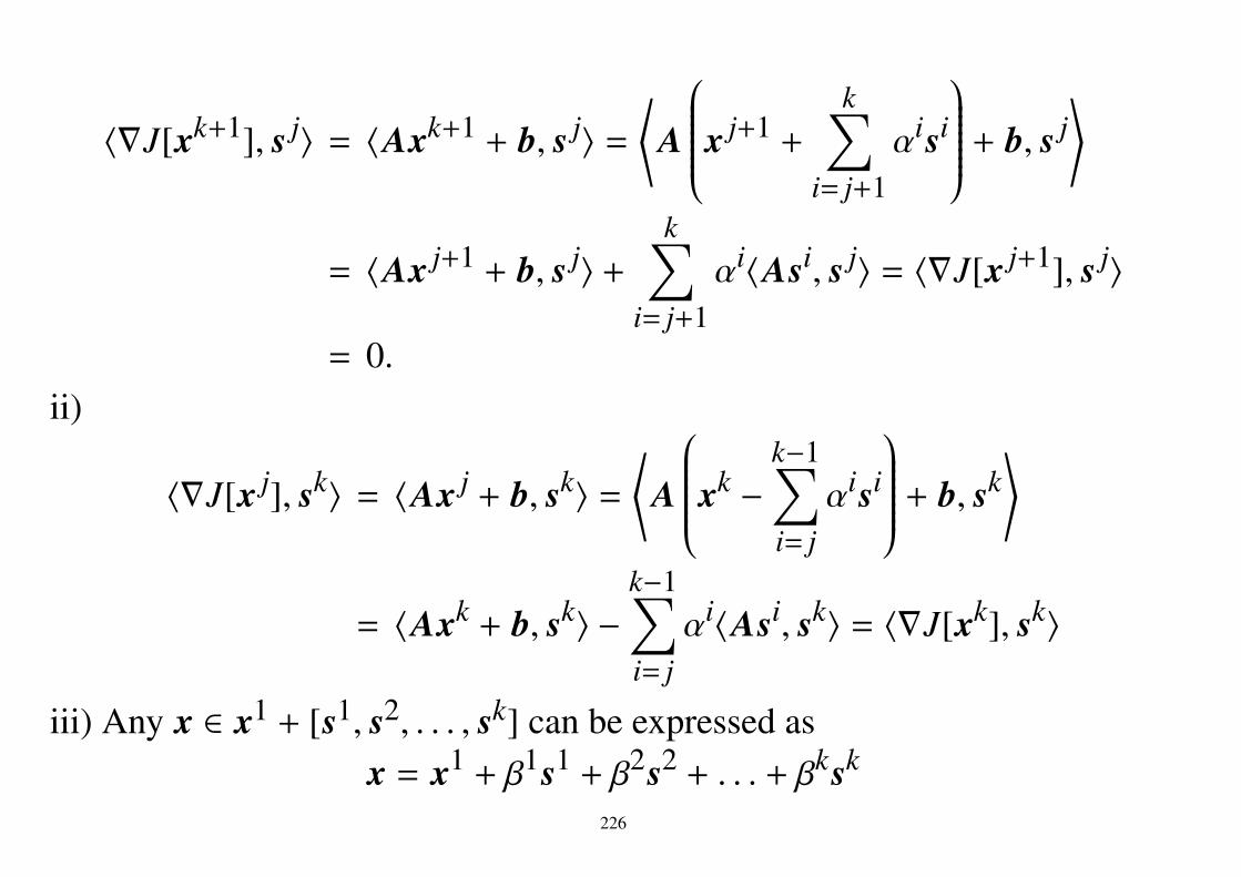
⟨∇J[xk+1], s j⟩ = ⟨Axk+1 + b, s j⟩ =⟨
A
x j+1 +k∑
i= j+1αisi
+ b, s j⟩
= ⟨Ax j+1 + b, s j⟩ +k∑
i= j+1αi⟨Asi, s j⟩ = ⟨∇J[x j+1], s j⟩
= 0.ii)
⟨∇J[x j], sk⟩ = ⟨Ax j + b, sk⟩ =⟨
A
xk −k−1∑i= j
αisi
+ b, sk⟩
= ⟨Axk + b, sk⟩ −k−1∑i= j
αi⟨Asi, sk⟩ = ⟨∇J[xk], sk⟩
iii) Any x ∈ x1 + [s1, s2, . . . , sk] can be expressed asx = x1 + β1s1 + β2s2 + . . . + βksk
226

with β1, β2, . . . , βk ∈ R. Then,
J(x) =12
⟨x1 +
k∑i=1
βisi, A
x1 +k∑
i=1βisi
⟩+
⟨b, x1 +
k∑i=1
βisi⟩+ c
=12
⟨x1, Ax1
⟩+
12
⟨x1,
k∑i=1
βi Asi⟩+
12
⟨ k∑i=1
βisi, Ax1⟩
+12
⟨ k∑i=1
βisi,k∑
i=1βi Asi
⟩+ ⟨b, x1⟩ +
⟨b,
k∑i=1
βisi⟩+ c
=12
k∑i=1
k∑j=1
βiβ j⟨si, As j⟩ +k∑
i=1βi⟨Ax1 + b, si⟩ + 1
2⟨x1, Ax1⟩ + ⟨b, x1⟩ + c
=
k∑i=1
[12⟨si, Asi⟩(βi)2 + ⟨Ax1 + b, si⟩βi
]+
12⟨x1, Ax1⟩ + ⟨b, x1⟩ + c.
227

Therefore, it becomes minimum if and only if
βi = −⟨Ax1 + b, si⟩⟨si, Asi⟩
. (160)
Since Ax1 + b = ∇J[x1], Axi + b = ∇J[xi], (ii) in Theorem 9 yields that
αi = −⟨Axi + b, si⟩⟨si, Asi⟩
= −⟨∇J[xi], si⟩⟨si, Asi⟩
= −⟨∇J[x1], si⟩⟨si, Asi⟩
= −⟨Ax1 + b, si⟩⟨si, Asi⟩
= βi.
(161)Since
xk+1 = x1 +k∑
i=1αisi = x1 +
k∑i=1
βisi, (162)
xk+1 minimizes J(x) in x1 + [s1, . . . , sk]. QED.
Since we have x1 + [s1, . . . , sn] = Rn, then xn+1 minimizes J(x) in Rn.
228

How to calculate s1, s2, . . . , sk. s1 is given by the gradient of J at x1.
s1 = −∇J[x1]. (163)
And we assume that
sk+1 = −∇J[xk+1] +k∑
j=1λk+1
j s j. (164)
Since sk+1 and s j ( j = 1, 2, . . . , k) are A-conjugate,
0 = ⟨sk+1, As j⟩ =⟨−∇J[xk+1] +
k∑i=1
λki si, As j
⟩= −⟨∇J[xk+1], As j⟩ + λk+1
j ⟨sj, As j⟩.
Then, we have
λk+1j =
⟨∇J[xk+1], As j⟩⟨s j, As j⟩
.
229
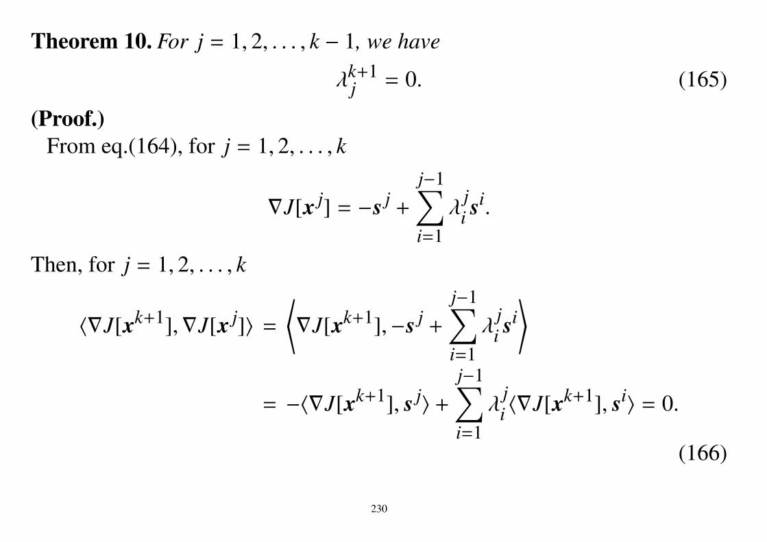
Theorem 10. For j = 1, 2, . . . , k − 1, we have
λk+1j = 0. (165)
(Proof.)From eq.(164), for j = 1, 2, . . . , k
∇J[x j] = −s j +
j−1∑i=1
λji si.
Then, for j = 1, 2, . . . , k
⟨∇J[xk+1],∇J[x j]⟩ =⟨∇J[xk+1],−s j +
j−1∑i=1
λji si
⟩
= −⟨∇J[xk+1], s j⟩ +j−1∑i=1
λji ⟨∇J[xk+1], si⟩ = 0.
(166)
230

Since
∇J[x j+1] − ∇J[x j] = Ax j+1 + b − (Ax j + b) = A(x j+1 − x j)= A(x j + α js j − x j) = α j As j,
we have
As j =∇J[x j+1] − ∇J[x j]
α j . (167)
For j = 1, 2, . . . , k − 1, eq.(166) yields
λk+1j =
⟨∇J[xk+1], As j⟩⟨s j, As j⟩
=⟨∇J[xk+1],∇J[x j+1] − ∇J[x j]⟩
α j⟨s j, As j⟩
=⟨∇J[xk+1],∇J[x j+1]⟩
α j⟨s j, As j⟩− ⟨∇J[xk+1],∇J[x j]⟩
α j⟨s j, As j⟩= 0.
QED.
Since λk+11 = λk+1
2 = · · · = λk+1k−1 = 0, we define λk by
λk = λk+1k .
231

Algorithm of conjugate gradient method for a quadratic function.
1. x1 : initial vector,s1 = −(Ax1 + b),k = 1.
2. if ∥Axk + b∥ is enough small, stop.
3. αk = −⟨Axk+b,sk⟩⟨sk,Ask⟩ .
4. xk+1 = xk + αksk.
5. λk = ⟨Axk+1+b,Ask⟩⟨sk,Ask⟩ .
6. sk+1 = −Axk+1 − b + λksk.
7. k = k + 1.
8. go to 2.
232

10.1.3 Conjugate gradient method for non-quadratic functionExtension to a non-quadratic case.
• αk can be obtained by linear search (xk+1 = xk + αksk).•We can use ∇J.• However, we cannot use Ask . Then, λk cannot be obtained.
Theorem 11. (Fletcher-Reeves’ equation)When J is a quadratic function, we have
λk =∥∇J[xk+1]∥2
∥∇J[xk]∥2
233

(Proof.)From eq.(167), we have
αk⟨sk, Ask⟩ = ⟨sk,∇J[xk+1] − ∇J[xk]⟩= ⟨sk,−∇J[xk]⟩= ⟨−∇J[xk] + λk−1sk−1,−∇J[xk]⟩= ∥∇J[xk]∥2, (168)
and eq.(166) yield
⟨∇J[xk+1],∇J[xk+1] − ∇J[xk]⟩ = ∥∇J[xk+1]∥2. (169)
Then, we have
λk =⟨∇J[xk+1],∇J[xk+1] − ∇J[xk]⟩
αk⟨sk, Ask⟩=∥∇J[xk+1]∥2
∥∇J[xk]∥2. (170)
234

Algorithm of conjugate gradient method for a non-quadratic function.
1. x1 : initial vector,s1 = −∇J[x1],k = 1.
2. if ∇J[xk] is enough small, stop.
3. Solve linear search problem with respect to αk:
F(αk) = J(xk + αksk)
and letxk+1 = xk + αksk
4. λk = ∥∇J[xk+1]∥2∥∇J[xk]∥2
5. sk+1 = −∇J[xk+1] + λksk
6. k = k + 1.
7. go to 2.
235
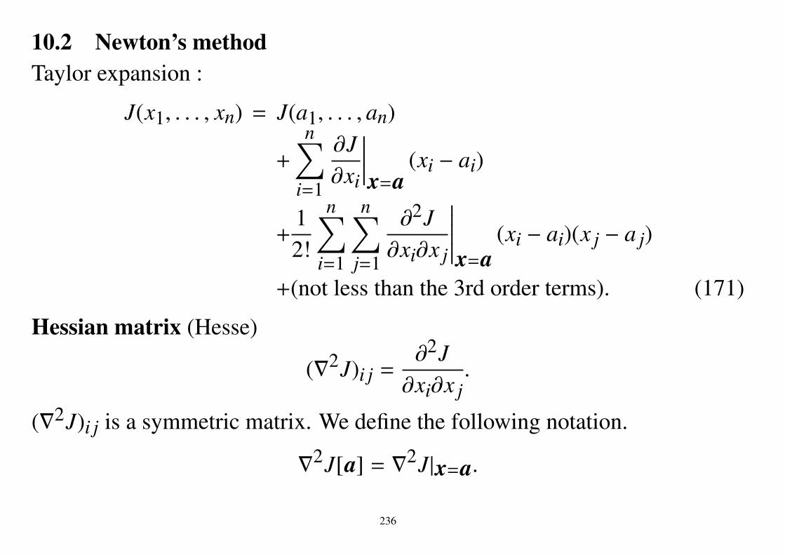
10.2 Newton’s methodTaylor expansion :
J(x1, . . . , xn) = J(a1, . . . , an)
+
n∑i=1
∂J∂xi
∣∣∣∣∣x=a(xi − ai)
+12!
n∑i=1
n∑j=1
∂2J∂xi∂x j
∣∣∣∣∣∣x=a(xi − ai)(x j − a j)
+(not less than the 3rd order terms). (171)
Hessian matrix (Hesse)
(∇2J)i j =∂2J∂xi∂x j
.
(∇2J)i j is a symmetric matrix. We define the following notation.
∇2J[a] = ∇2J|x=a.
236

Eq.(171) can be described as
J(x) = J(a) + ⟨∇J[a], x − a⟩ + 12!⟨x − a,∇2J[a](x − a)⟩ + · · · .
We define J2 that is an approximation of J with a quadratic function as
J2(x) = J(a) + ⟨∇J[a], x − a⟩ + 12!⟨x − a,∇2J[a](x − a)⟩.
If ∇2J[a] > 0, the minimum point of J2(x) is given as
xmin = −(∇2J[a])−1(∇J[a] − (∇2J[a])a)= a − (∇2J[a])−1∇J[a]. (172)
237

Newton’s method
238

Algorithm of Newton’s method
1. x1 : initial vector,k = 1
2. Calculate ∇J[xk] and ∇2J[xk].
3. If ∥∇J[xk]∥ is small, then stop
4. xk+1 = xk − (∇2J[xk])−1∇J[xk]
5. k = k + 1
6. go to 2.
This method is equivalent to the Newton-Raphson method for solving thefollowing equation:
∇J[x] = 0. (173)
239

10.2.1 Quasi Newton’s methodHk : a matrix that approximates the inverse of a Hessian matrix, (∇2J)−1.
Algorithm of Quasi Newton’s method (except for obtaining Hk)
1. x1 : initial vector (H1 = I, k = 1)
2. Calculate ∇J[xk].
3. If ∥∇J[xk]∥ is small, stop.
4. sk = −Hk∇J(xk) : the direction for linear search.
5. Solve the linear search problem of
F(αk) = J(xk + αksk)
αand letxk+1 = xk + αksk
6. Calculate Hk+1 by using (xk+1 − xk), (∇J[xk+1] − ∇J[xk]), and Hk.
7. k = k + 1 and go to 2.240

Condition for obtaining Hk :Let
pk = xk+1 − xk = αksk, (174)qk = ∇J[xk+1] − ∇J[xk]. (175)
Consider the case that J is a quadratic function, that is
J(x) =12⟨x, Ax⟩ + ⟨b, x⟩ + c. (176)
Then,
qk = Axk+1 + b − (Axk + b) = A(xk+1 − xk) = ∇2J[xk]pk. (177)
If there exists the inverse of ∇2J[x], we have
(∇2J[xk])−1qk = pk. (178)
241

Quasi-Newton condition for Hk+1
Hk+1qk = pk. (179)
Theorem 12. Assume that
J(x) =12⟨x, Ax⟩ + ⟨b, x⟩ + c. (180)
Let xk be the result of Quasi-Newton’s method at the k-th iteration. We assumethat A and Hk (k = 1, 2, . . . , n) are positive definite (n,n)-matrices and
∇J(xk) , 0 k = 1, 2, . . . , n, (181)Hk+1q j = p j j = 1, 2, . . . , k, k = 1, 2, . . . , n. (182)
Then the following relations hold.
(i) s1, . . . , sn are A-conjugate and linearly independent. (sk = −Hk∇J[xk])(ii) xn+1 is the minimum point of J and
Hn+1 = A−1.
242

(Proof.)Since J is a quadratic function, it follows that
q j = Ax j+1 + b − (Ax j + b) = α j As j, (183)
andp j = x j+1 − x j = α js j. (184)
Eq.(182) yields that
α js j = p j = Hk+1q j = Hk+1α j As j = α jHk+1 As j.
Then, we haveHk+1 As j = s j ( j = 1, 2, . . . , k). (185)
(i)
s1 = −H1∇J[x1] = −(Ax1 + b),s2 = −H2∇J[x2] = −H2(Ax2 + b).
243

It follows that
⟨s2, As1⟩ = ⟨−H2∇J[x2], As1⟩ = −⟨Ax2 + b,H2 As1⟩ = −⟨Ax2 + b, s1⟩= −⟨A(x1 + α1s1) + b, s1⟩ = −α1⟨s1, As1⟩ − ⟨Ax1 + b, s1⟩
=⟨Ax1 + b, s1⟩⟨s1, As1⟩
⟨s1, As1⟩ − ⟨Ax1 + b, s1⟩ = 0.
Suppose that s1 and s2 are not linearly independent, A > 0 and ⟨s2, As1⟩ = 0yield that s1 = 0 or s2 = 0. Since we assume that Hk > 0, this contradicts to∇J[x1] , 0 and ∇J[x2] , 0. Then, s1 and s2 are linearly independent.
Assume that s1, . . . , sk are A-conjugate and linearly independent. Sinces1, . . . , sk are A-conjugate, Theorem 9 yields
⟨∇J[xk+1], s j⟩ = 0 ( j = 1, 2, . . . , k).
Eq.(185) yields that for j = 1, 2, . . . , k
⟨sk+1, As j⟩ = ⟨−Hk+1∇J[xk+1], As j⟩ = −⟨∇J[xk+1], Hk+1 As j⟩= −⟨∇J[xk+1], s j⟩ = 0.
Then, s1, . . . , sk+1 are A-conjugate. (mathematical induction)244

Suppose that s1, . . . , sk+1 are not linearly independent. Then, for real num-bers λ1, . . . , λk+1 we have
k+1∑i=1
λisi = 0.
Then,
0 =⟨
Ask+1,k+1∑i=1
λisi⟩=
k+1∑i=1
λi⟨sk+1, Asi⟩ = λk+1⟨sk+1, Ask+1⟩,
and A > 0 yield that λk+1 = 0. It follows thatk∑
i=1λisi = 0.
This contradicts the assumption that s1, . . . , sk are linearly independent. Themathematical induction yields (i).
245

(ii)From (iii) in Theorem 9 and (i), we can know that xn+1 is the minimum
point of J. Since for i = 1, 2, . . . , n
Hn+1 Asi = si,
and s1, . . . , sn are linearly independent, we have
Hn+1 A = I,Hn+1 = A−1.
QED.
Problem 20. Prove that a positive definite (N,N)-matrix A is regular (it hasa inverse matrix).
Hint: First, prove that Ax = 0 implies x = 0. This implies A is an injector.Second, for a basis eiNi=1 in RN, prove AeiNi=1 is also a basis in RN. Thisimplies A is an surjection. We can prove it by showing Aei (i = 1, 2, . . . ,N)are linearly independent (using ei (i = 1, 2, . . . ,N) are linearly independent).Then, because A is an injector and a surjection, it is regular.
246

10.2.2 Formula for obtaining Hk
We assume thatHk+1 = Hk + ∆Hk. (186)
Since it is preferable that the formula for ∆Hk is simple, we consider the casethat the rank of ∆HK is 1 or 2.Formula of rank 1 We can let
∆Hk = αuk(uk)T
for a real number α and a vector uk. The quasi-Newton condition yields that
Hkqk + αuk(uk)T qk = pk. (187)
Then, we haveα⟨uk, qk⟩uk = pk − Hkqk. (188)
In order to satisfy this equation, we let
uk = pk − Hkqk, (189)α = 1/⟨uk, qk⟩. (190)
247

It follows that
Hk+1 = Hk +(pk − Hkqk)(pk − Hkqk)T
⟨pk − Hkqk, qk⟩. (191)
This formula has a disadvantage that even if Hk > 0, Hk+1 may not bepositive definite when it happens ⟨pk − Hkqk, qk⟩ < 0.
Formula of rank 2 (Davidon-Fletcher-Powell (DFP) formula)Let
∆HK = αuk(uk)T + βvk(vk)T .
The quasi-Newton condition yields that
Hkqk + αuk(uk)T qk + βvk(vk)T qk = pk. (192)
Then, we have
Hkqk + α⟨uk, qk⟩uk + β⟨vk, qk⟩vk = pk. (193)
248
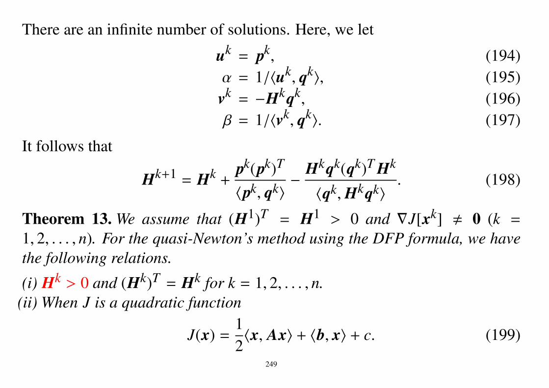
There are an infinite number of solutions. Here, we let
uk = pk, (194)α = 1/⟨uk, qk⟩, (195)
vk = −Hkqk, (196)β = 1/⟨vk, qk⟩. (197)
It follows that
Hk+1 = Hk +pk(pk)T
⟨pk, qk⟩− Hkqk(qk)T Hk
⟨qk, Hkqk⟩. (198)
Theorem 13. We assume that (H1)T = H1 > 0 and ∇J[xk] , 0 (k =1, 2, . . . , n). For the quasi-Newton’s method using the DFP formula, we havethe following relations.
(i) Hk > 0 and (Hk)T = Hk for k = 1, 2, . . . , n.(ii) When J is a quadratic function
J(x) =12⟨x, Ax⟩ + ⟨b, x⟩ + c. (199)
249

s1, . . . , sn are A-conjugate to each other and
Hk+1q j = p j (200)
for j = 1, 2, . . . , k and k = 1, 2, . . . , n.
(Proof.)(i) (Hk)T = Hk is clear.
Assume that Hk > 0. We will prove Hk+1 > 0. There exists a symmetricpositive definite matrix Dk such that,
Hk = Dk Dk
We can write as H = U
λ1 0 · · ·· · · . . . · · ·0 · · · λn
UT with λi > 0 (i = 1, 2, . . . , n).
Let D = U
√λ1 0 · · ·· · · . . . · · ·0 · · ·
√λn
UT .
Since UUT = UT U = I, it is clear that D = DT and H = DD.250

For any z,
⟨z, Hk+1z⟩ = ⟨z, Hkz⟩ + ⟨z, pk(pk)T z⟩⟨pk, qk⟩
− ⟨z, Hkqk(qk)T Hkz⟩⟨qk, Hkqk⟩
= ⟨z, Dk Dkz⟩ + ⟨z, pk⟩2
⟨pk, qk⟩− ⟨z, Hkqk⟩2
⟨qk, Dk Dkqk⟩
= ∥Dz∥2 − ⟨Dkz, Dkqk⟩2
∥Dkqk∥2+⟨z, pk⟩2
⟨pk, qk⟩
=∥Dkz∥2∥Dkqk∥2 − ⟨Dkz, Dkqk⟩2
∥Dkqk∥2+⟨z, pk⟩2
⟨pk, qk⟩
≥ ⟨z, pk⟩2
⟨pk, qk⟩(201)
If pk = 0, then 0 = pk/αk = sk = Hk∇J[xk]. Since Hk > 0, ∇J[xk] = 0.
This contradiction yields pk , 0.If qk = 0, then ∇J[xk+1] = ∇J[xk]. Let F(t) = J[xk + tsk].
251

Since t = αk is an extreme point of F(t), we have
0 =dFdt
∣∣∣∣∣t=αk= ⟨sk,∇J[xk + αksk]⟩ = −⟨Hk∇J[xk],∇J[xk+1]⟩. (202)
Then, ∇J[xk+1] = ∇J[xk] yields
⟨∇J[xk+1], Hk∇J[xk]⟩ = ⟨∇J[xk], Hk∇J[xk]⟩ = 0. (203)
This contradicts that ∇J[xk] , 0 and Hk > 0. Then, qk , 0.Since
dFdt
∣∣∣∣∣t=0= ⟨sk,∇J[xk]⟩ = −⟨Hk∇J[xk],∇J[xk]⟩ < 0,
t = 0 is not the minimum point and we have αk > 0. Then, eq.(202) yields
⟨pk, qk⟩ = ⟨αksk,∇J[xk+1] − ∇J[xk]⟩ = −αk⟨∇J[xk], sk⟩= αk⟨∇J[xk], Hk∇J[xk]⟩ > 0. (204)
Therefore,⟨z, Hk+1z⟩ ≥ 0.
252

Assume that ⟨z, Hk+1z⟩ = 0. From eq.(201), we have ⟨z, pk⟩ = 0 and|⟨Dkz, Dkqk⟩| = ∥Dkz∥∥Dkqk∥ so that the equatity condition of the Cauchy-Schwartz’s inequality yields
Dkz = βDkqk
with a real number β. Since Dk > 0, we have
z = βqk.
Since ⟨z, pk⟩ = 0 yields β⟨pk, qk⟩ = 0. Then, eq.(204) yields that β = 0 andz = βqk = 0. Therefore, we have Hk+1 > 0.
(ii) From the definition we have
H2 = I +p1(p1)T
⟨p1, q1⟩− q1(q1)T
⟨q1, q1⟩.
Then,H2q1 = q1 + p1 − q1 = p1.
253

We assume that s1, . . . , sk are A-conjugateHk+1q j = p j ( j = 1, 2, . . . , k)
,
and will prove that s1, . . . , sk+1 are A-conjugateHk+2ql = pl (l = 1, 2, . . . , k + 1)
.
From (i) in Theorem 9, for j = 1, 2, . . . , k we have
α j⟨sk+1, As j⟩ = ⟨−Hk+1∇J[xk+1], A(α js j)⟩ = −⟨Hk+1∇J[xk+1], Ap j⟩= −⟨∇J[xk+1], Hk+1 Ap j⟩ = −⟨∇J[xk+1], Hk+1q j⟩= −⟨∇J[xk+1], p j⟩ = −α j⟨∇J[xk+1], s j⟩ = 0. (205)
Since α j , 0, ⟨sk+1, As j⟩ = 0 for j = 1, 2, . . . , k. Then, s1, s2, . . . , sk, sk+1 areA-conjugate.
254

For j = 1, 2, . . . , k we have
⟨pk+1, q j⟩ = ⟨pk+1, Ap j⟩ = αk+1α j⟨sk+1, As j⟩ = 0 (206)⟨qk+1, Hk+1q j⟩ = ⟨qk+1, p j⟩ = ⟨Apk+1, p j⟩ = αk+1α j⟨sk+1, As j⟩ = 0.
(207)
Then,
Hk+2q j = Hk+1q j +⟨pk+1, q j⟩⟨pk+1, qk+1⟩
pk+1 − ⟨qk+1, Hk+1q j⟩
⟨qk+1, Hk+1qk+1⟩Hk+1qk+1
= Hk+1q j = p j. (208)
Furthermore,
Hk+2qk+1 = Hk+1qk+1 + pk+1 − Hk+1qk+1 = pk+1. (209)
This completes the proof. QED.
Note that (i) holds for not-quadratic problems.
255

Broyden-Fletcher-Goldfarb-Shannon (BFGS) formula
This formula is now the most popular.
Hk+1 =pk(pk)T
⟨pk, qk⟩+
I − pk(qk)T
⟨pk, qk⟩
HkI − pk(qk)T
⟨pk, qk⟩
(210)
256

11 Conditional Optimization Problemf : Rn → R : a function to be optimizatedg : Rn → Rm : a vector of functions for condition
g(x) = (g1(x), g2(x), . . . , gm(x))T
Equality condition:subject to g(x) = 0,minimize f (x).
Inequality condition:subject to g(x) ≥ 0,minimize f (x).
• m : the number of conditions.• g(x) ≥ 0 is equivalent to g1(x) ≥ 0, g2(x) ≥ 0,. . ., gm(x) ≥ 0.• An equality condition can be transformed to inequality conditions
subject to g(x) ≥ 0,−g(x) ≥ 0,
minimize f (x).
257

Conditional Optimization
258

11.1 Lagrange’s method of undetermined coefficientsProblem : (Equality conditions)
Subject to g1(x1, x2, . . . , xn) = 0,
· · ·gm(x1, x2, . . . , xn) = 0,
(211)
minimizef (x1, x2, . . . , xn) (212)
where f , g1, . . . , gm are continuously differentiable. Let
A =
∂g1∂x1· · · ∂gm
∂x1· · · · · · · · ·∂g1∂xn· · · ∂gm
∂xn
(213)
259

Theorem 14. (Lagrange’s method of undetermined coefficients)Assume that rank(A) = m for every (x1, . . . , xn) satisfying eq.(211). If
(x1, . . . , xn) is a stationary point of f among those satisfying eq.(211), thenthe differentials of
J(x1, . . . , xn, λ1, . . . , λm)= f (x1, . . . , xn) − λ1g1(x1, . . . , xn) − · · · − λmgm(x1, . . . , xn) (214)
with respect to x1, . . . , xn, λ1, . . . , and λm are 0.
λ1, . . . , λm are called the Lagrange’s (undetermined) coefficients.
(Proof.)We use the following Implicit function theorem.
(As for its proof, see a textbook of Calculus.)
260

Proposition 1. Assume that x = a = (a1, . . . , an) satisfies eq.(211) and
det
∂g1∂x1
∣∣∣∣x=a · · ·∂gm∂x1
∣∣∣∣x=a· · · · · · · · ·
∂g1∂xm
∣∣∣∣x=a · · ·∂gm∂xm
∣∣∣∣x=a
, 0. (215)
Then, there exist continuously differentiable functions
h1(xm+1, . . . , xn), . . . , hm(xm+1, . . . , xn)
on a neighborhood of (am+1, . . . , an) such that
g j(h1(xm+1, . . . , xn), . . . , hm(xm+1, . . . , xn), xm+1, . . . , xn) = 0 (216)
for all j = 1, 2, . . . ,m. Furthermore, any (x1, . . . , xn) satisfying eq.(211) onthe neighborhood of a can be written as
(h1(xm+1, . . . , xn), . . . , hm(xm+1, . . . , xn), xm+1, . . . , xn)
261

ExampleFor a function g(x1, x2), weassume that g(a1, a2) = 0and
∂g∂x1
∣∣∣∣∣∣x1=a1,x2=a2
, 0.
Then there exist a functiony = f (x2) in the neighbor-hood of x2 = a2 such that
g( f (x2), x2) = 0.
g(x1, x2) expresses implic-itly a function y = f (x2).
262

Since rank(A) = m, by exchanging variables (rows in A), we can assumethat eq.(215) holds at a stationary point. Then, we have hi(xm+1, . . . , xn) (i =1, 2, . . . ,m) satisfying eq.(216). We define F(xm+1, . . . , xn) and G j(xm+1, . . . , xn)as
F(xm+1, . . . , xn)= f (h1(xm+1, . . . , xn), . . . , hm(xm+1, . . . , xn), xm+1, . . . , xn), (217)
G j(xm+1, . . . , xn)= g j(h1(xm+1, . . . , xn), . . . , hm(xm+1, . . . , xn), xm+1, . . . , xn) (218)
for j = 1, 2, . . . ,m. Then, we have
G j(xm+1, . . . , xn) = 0. (219)
for any (xm+1, . . . , xn) in the neighborhood of the stationary point. We alsohave
∂F∂xk= 0 (220)
at the stationary point for k = m + 1, . . . , n.
263

Eqs.(220) and (219) yield that
∂F∂xk=
m∑i=1
∂ f∂xi
∂hi∂xk+∂ f∂xk= 0, (221)
∂G j
∂xk=
m∑i=1
∂g j
∂xi
∂hi∂xk+∂g j
∂xk= 0. (222)
for j = 1, 2, . . . ,m and k = m + 1, . . . , n.By using matrices, we can describe the equations as
∂F∂xm+1...∂F∂xn
=
∂h1∂xm+1
· · · ∂hm∂xm+1
· · · · · · · · ·∂h1∂xn
· · · ∂hm∂xn
∂ f∂x1...∂ f∂xm
+
∂ f∂xm+1...∂ f∂xn
= 0, (223)
264

and ∂G1∂xm+1
· · · ∂Gm∂xm+1
· · · · · · · · ·∂G1∂xn
· · · ∂Gm∂xn
=
∂h1∂xm+1
· · · ∂hm∂xm+1
· · · · · · · · ·∂h1∂xn
· · · ∂hm∂xn
∂g1∂x1· · · ∂gm
∂x1· · · · · · · · ·∂g1∂xm· · · ∂gm
∂xm
+
∂g1∂xm+1
· · · ∂gm∂xm+1
· · · · · · · · ·∂g1∂xn
· · · ∂gm∂xn
= O. (224)
Let
H =
∂h1∂xm+1
· · · ∂hm∂xm+1
· · · · · · · · ·∂h1∂xn
· · · ∂hm∂xn
,
265

p =
∂ f∂x1...∂ f∂xm
p′ =
∂ f
∂xm+1...∂ f∂xn
,and
Q =
∂g1∂x1· · · ∂gm
∂x1· · · · · · · · ·∂g1∂xm· · · ∂gm
∂xm
Q′ =
∂g1∂xm+1
· · · ∂gm∂xm+1
· · · · · · · · ·∂g1∂xn
· · · ∂gm∂xn
Then, eqs.(221) and (222) can be written as
Hp+ p′ = 0, (225)HQ + Q′ = O. (226)
Since Q is regular matrix, let
λ =
λ1...λm
= Q−1 p. (227)
266

From eq.(226), we haveH = −Q′Q−1. (228)
From eq.(225),0 = p′ + (−Q′Q−1)Qλ = p′ − Q′λ (229)
From p− Qλ = 0 and p′ − Q′λ = 0, it follows that∂J∂xk=∂ f∂xk− λ1
∂g1∂xk− · · · − λm
∂gm∂xk= 0 (230)
for k = 1, 2, . . . , n. Furthermore,∂J∂λl= −gl = 0 (231)
for l = 1, 2, . . . ,m. QED.
267

Lagrange’s method(n = 2 and m = 1 ⇒ ∇ f − λ∇g = 0 and g = 0)
268

Lagrange’s method
269

Example
g(x1, x2) = 2x1 + x2 − 1, (232)f (x1, x2) = x2
1 + 2x22. (233)
Since
A =(
21
)implies that rank(A) = 1, we can use
J = x21 + 2x2
2 − λ(2x1 + x2 − 1)
270

∂J∂x1= 2x1 − 2λ = 0
∂J∂x2= 4x2 − 2λ = 0
∂J∂λ= 2x1 + x2 + 1 = 0
The answer is given as x1 =49
x2 =19. (234)
271

Bad example
g(x1, x2) = (2x1 + x2 − 1)2, (235)f (x1, x2) = x2
1 + 2x22. (236)
LetJ = x2
1 + 2x22 − λ(2x1 + x2 − 1)2.
∂J∂x1= 2x1 − 4λ(2x1 + x2 − 1) = 0 (237)
∂J∂x2= 4x2 − 2λ(2x1 + x2 − 1) = 0 (238)
∂J∂λ= −(2x1 + x2 − 1)2 = 0 (239)
By substituting eq.(239) to eqs.(237) and (238), we havex1 = 0x2 = 0 . (240)
272

But eq.(239) implies
1 = 0 → contradiction.
This is because
A =(
4(2x1 + x2 − 1)2(2x1 + x2 − 1)
)=
(00
)when (x1, x2) satisfies eq.(239). (rank(A) = 0.)→ Lagrange’s method cannot be applied.
Problem 21. Solve the following optimization problem by Lagrange’s method.
g(x1, x2) = x1x2 − 1, (241)f (x1, x2) = x2
1 + 4x1x2 + 4x22. (242)
273

ExampleConsider the following optimization problem of a matrix B.
g(B) = BA − C, (243)f (B). (244)
NG:J(B) = f (B)−λtr((BA−C)(BA−C)T ) = f (B)−λ
∑i
∑j|(BA−C)i j|2 (245)
OK:
J(B) = f (B) − tr(Λ(BA − C)T ) = f (B) −∑
i
∑j
(Λ)i j(BA − C)i j (246)
The squared term cannot be used for the condition in Lagrange’s method.
However, we often use
J(x) = f (x) − λg(x) + a(g(x))2, (247)
where a is a constant to improve a stability of numerical calculation.274

11.2 Inequality conditionProblem: Subject to
g1(x1, x2, . . . , xn) ≥ 0,· · ·
gm(x1, x2, . . . , xn) ≥ 0,(248)
minimizef (x1, x2, . . . , xn), (249)
where f , g1, . . . , gm are continuously differentiable.
11.2.1 KKT (Karush-Kuhn-Tucker) conditionWe define Lagrange function as
J(x1, . . . , xn, λ1, . . . , λm)= f (x1, . . . , xn) − λ1g1(x1, . . . , xn) − · · · − λmgm(x1, . . . , xn) (250)
with Lagrange’s coefficients λ1, . . . , λm.
275

Theorem 15. (KKT condition)If (x1, . . . , xm) is a stationary point of f among those satisfying eq.(248),
then at the point we have∂J∂xi= 0 (251)
for i = 1, 2, . . . , n and we have
λ1 ≥ 0,· · ·λm ≥ 0,g1(x1, x2, . . . , xn) ≥ 0,· · ·gm(x1, x2, . . . , xn) ≥ 0,λ1g1(x1, x2, . . . , xn) = 0,· · ·λmgm(x1, x2, . . . , xn) = 0.
(252)
276

•When λi > 0,• gi(x) = 0.⇒ The minimum point is on the boundary of the condition by gi.
KKT condition277

•When λi = 0,• gi(x) ≥ 0.⇒ The minimum point is minimum without the condition of gi(x).
KKT condition278

11.3 Saddle point theorem and dual problem• Criteria (248) and (249) can be written as
min(x1,...,xn)
max(λ1≥0,...,λm≥0)
J(x1, . . . , xn, λ1, . . . , λm)
Remark: The number of variables increases but conditions becomes simple.(Proof)
We have
max(λ1≥0,...,λm≥0)
[f (x1, . . . , xn) − λ1g1(x1, . . . , xn) − · · · − λmgm(x1, . . . , xn)
]=
f (x1, . . . , xn) if g1(x1, . . . , xn) ≥ 0, . . . , gm(x1, . . . , xn) ≥ 0∞ else.
Since the above value is minimized with respect to x1, . . . , xn andf (x1, . . . , xn) < ∞, its minimum point has to satisfy conditionsg1(x1, . . . , xn) ≥ 0, . . . , gm(x1, . . . , xn) ≥ 0. QED.
279

Theorem 16. (Saddle point theorem) :We have
min(x1,...,xn)
max(λ1≥0,...,λm≥0)
J(x1, . . . , xn, λ1, . . . , λm)
= max(λ1≥0,...,λm≥0)
min(x1,...,xn)
J(x1, . . . , xn, λ1, . . . , λm).
(We can commute minimization and maximization.)
Remark : It does not hold if the domain of variables is discrete.
x \ λ 1 2 maxλ1 0.3 0.5 0.52 0.7 0.4 0.7
minx maxλ = 0.5minx 0.3 0.4 maxλminx = 0.4
280

Saddle point theorem
• By using the saddle point theorem, we can rewrite the primal problem toits dual problem.
281

11.4 Dual problem of linear programmingDefinition of a linear programming problem
x : n-dimensional variableA : (m, n)-matrixb : m-dimensional variablec : n-dimensional variableMinimize
⟨c, x⟩ (253)subject to
Ax − b ≥ 0 (254)x ≥ 0 (255)
Let y = (y1, y2, · · · , ym)T is the vector of Lagrange’s undetermined coeffi-cients. Lagrange’s function can be written by
J(x, y) = ⟨c, x⟩ − y1(Ax − b)1 − · · · − ym(Ax + b)m (256)= ⟨c, x⟩ − ⟨y, Ax + b⟩. (257)
282

Then, the conditional optimization problem can be solved by
minx≥0
maxy≥0
J(x, y).
Since we haveminx f (x) = −maxx (− f (x))
From the saddle point theorem we have
minx≥0
maxy≥0
J(x, y) = maxy≥0
minx≥0
J(x, y) = −miny≥0
maxx≥0
(−J(x, y)) . (258)
Since we have
−J(x, y) = −⟨c, x⟩ + ⟨y, Ax⟩ + ⟨y, b⟩= ⟨y, b⟩ − ⟨x, (−AT y + c)⟩, (259)
eq.(258) is given by
−miny≥0
maxx≥0
(⟨y, b⟩ − x1(−AT y + c)1 − · · · − xn(−AT y + c)n
). (260)
283
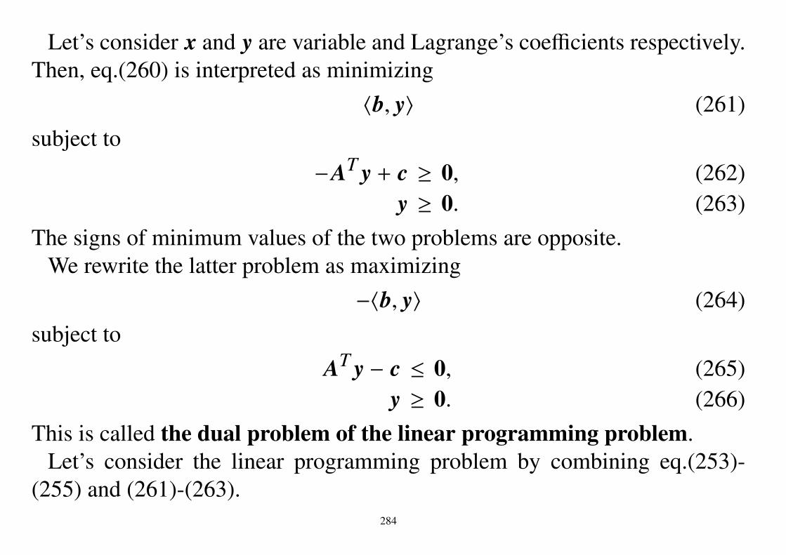
Let’s consider x and y are variable and Lagrange’s coefficients respectively.Then, eq.(260) is interpreted as minimizing
⟨b, y⟩ (261)subject to
−AT y + c ≥ 0, (262)y ≥ 0. (263)
The signs of minimum values of the two problems are opposite.We rewrite the latter problem as maximizing
−⟨b, y⟩ (264)subject to
AT y − c ≤ 0, (265)y ≥ 0. (266)
This is called the dual problem of the linear programming problem.Let’s consider the linear programming problem by combining eq.(253)-
(255) and (261)-(263).284

Minimize⟨c, x⟩ + ⟨b, y⟩ (267)
subject toAx − b ≥ 0, −AT y + c ≥ 0, x ≥ 0, y ≥ 0. (268)
Because x and y at the solution of the primal problem coincide with thoseof the dual problem, this problem is minimized if and only if both problemsare minimized. Since the signs of minimum values of eq.(253) and (261)are opposite, the minimum value of eq.(267) has to be zero. Therefore, theminimization problem can be solved by
⟨c, x⟩ + ⟨b, y⟩ = 0, Ax − b ≥ 0, −AT y + c ≥ 0, x ≥ 0, y ≥ 0. (269)
The linear programming problem is transformed to a system of linearinequalities.
285

11.5 Penalty method11.5.1 External penalty methodEquality condition
subject to g(x) = 0,minimize f (x).
Letψ1(t) = |t|, (270)
and we defineJ1(x; µ) = f (x) + µψ1(g(x)) (271)
Algorithm1. µ : initial positive value.
2. minimize J(x, µ) with respect to x.
3. increase µ.
4. go to 2.
286

Inequality condition:subject to g(x) ≥ 0,minimize f (x).
Let
ψ2(t) =
0 (t ≥ 0),−t (t < 0), (272)
and we defineJ2(x; µ) = f (x) + µψ2(g(x)). (273)
287

µ = 0
µ : small µ : largeExternal penalty method for inequality condition
288

11.5.2 Internal penalty methodInequality condition:
subject to g(x) ≥ 0,minimize f (x).
Letψ3(t) = 1/t (274)
for t > 0 and we define
J3(x; µ) = f (x) + µψ3(g(x)). (275)
Algorithm1. µ : initial positive value.
2. minimize J(x, µ) with respect to x.
3. decrease µ > 0.
4. go to 2.
289

µ : large µ : smallInternal penalty method for inequality condition
290

11.6 Example : Support Vector Machine (SVM)11.6.1 Optimum hyperplane classifier (OHC)• SVM, OHC : Two-class-classifier• A pattern belongs to one of two classes labeled by +1 or −1.• Ω+1,Ω−1 : The set of all patterns of which label is +1 and −1, respectively.• The classification function of OHC :
d(z) = ⟨w, z⟩ + θ (276)
with a vector w and a scalar θ.• Linear classifier
For an input vector z,d(z) > 0 z is classified to Ω+1d(z) < 0 z is classified to Ω−1
• The boundary for classification is a hyperplane perpendicular to w.• zl, ylLl=1 : Training data.
zl : Training patternyl : the label of .
291

First we assume that zl, ylLl=1 can be classified linearly.
• That is, there exist w and θ such that⇔d(zl) ≥ 1 if yl = 1,
d(zl) ≤ −1 if yl = −1.
(d(z) = ⟨w, z⟩ + θ)• It can be rewritten as for any l
yl d(zl) ≥ 1
oryl (⟨w, zl⟩ + θ) ≥ 1 (277)
• The margin of d(z) is defined as the half of the distance between the hy-perplanes of d(z) = 1 and d(z) = −1.• The margin M is given as
M =1∥w∥
292

Optimum hyper plane classifier
293

Maximization of margin
294

•Maximizing the margin, a basic optimization problem of OHC is given asSubject to
yl(⟨w, zl⟩ + θ) − 1 ≥ 0 (l = 1, 2, . . . L) (278)Minimize
∥w∥2 (279)
11.6.2 Soft margin• The training patterns may not be linearly separable.• It may be better to increase the margin even if it provides an incorrect
answer to a small number of training patters.•We introduce variables ξl ≥ 0 (l = 1, 2, . . . , L) to weaken the condition as
yl(⟨w, zl⟩ + θ) ≥ 1 − ξl. (280)
• If ξl = 0, eq.(280) is equivalent to eq.(277).• If ξl > 0, the margin is soften for the zl.• Especially if ξl > 1, the training pattern may be misclassified.⇒We have to introduce an optimum condition, which makes ξl smaller.
295
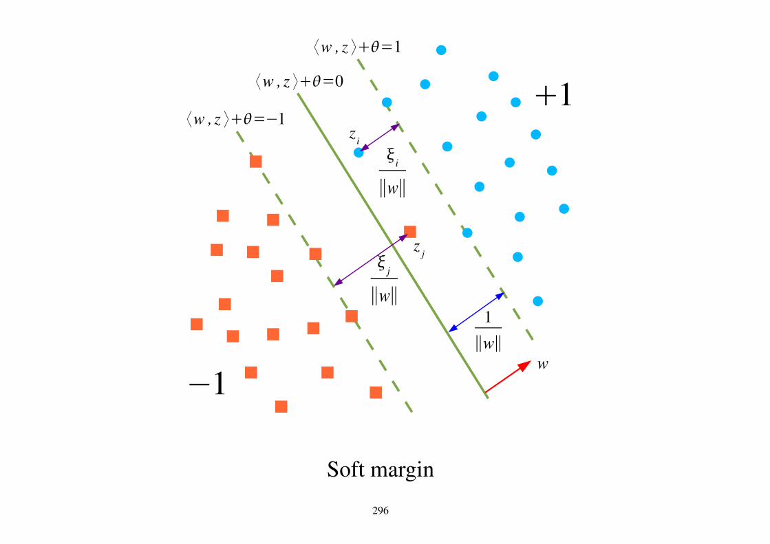
Soft margin
296

Maximum margin without soft margin
297

No feasible solution without soft margin
298

• The optimization problem with respect to w and θ for learning is given asSubject to
yl(⟨w, zl⟩ + θ) − 1 + ξl ≥ 0 (281)ξl ≥ 0 (282)
Minimize12∥w∥2 +C
L∑l=1
ξl (283)
where C is a constant.• The smaller C is, the softer the margin is.
The number of misclassified training patterns is increased.
299

11.6.3 Solution of OHCLagrange function :
LP =12∥w∥2 +C
L∑k=1
ξk −L∑
k=1µkξk −
L∑k=1
αkyk(⟨w, zk⟩ + θ) − 1 + ξk, (284)
where α1, α2 . . . , αL, µ1, µ2 . . . , µL are Lagrange’s coefficients.
• Saddle point theorem yields
minw, θ, ξ
maxα≥0, µ≥0
LP = maxα≥0, µ≥0
minw, θ, ξ
LP,
where α ≥ 0 and µ ≥ 0 implies α1 ≥ 0, . . . , αL ≥ 0 and µ1 ≥ 0, . . . , µL ≥ 0,respectively.• There is no condition for minimizing w = (w1, . . . ,wN), θ, and ξ = (ξ1, . . . , ξL).• The minimization can be done by letting the partial derivatives with respect
to w1, . . . ,wN, θ, ξ1, . . . , ξL to be zero.
300

• Then, we have
∂LP∂wn
= wn −L∑
k=1αkyk(zk)n = 0 (285)
∂LP∂θ= −
L∑k=1
αkyk = 0 (286)
∂LP∂ξl= C − µl − αl = 0 (287)
301

•We substitute them in to eq.(284)
LP =12
⟨ L∑l=1
αlylzl,L∑
k=1αkykzk
⟩+
L∑k=1
ξk(C − µk − αk)
−L∑
k=1αkyk
⟨ L∑l=1
αlylzl, zk
⟩−
L∑k=1
αkykθ +L∑
k=1αk
=
L∑k=1
αk −12
L∑l=1
L∑k=1
αlαkykyl⟨zl, zk ⟩ ≡ LD (288)
•We can obtain the dual problem LD.• In order to obtain SVM, we have to solve
maxα≥0, µ≥0
LD
under the conditions eqs.(285), (286), and (287).
302
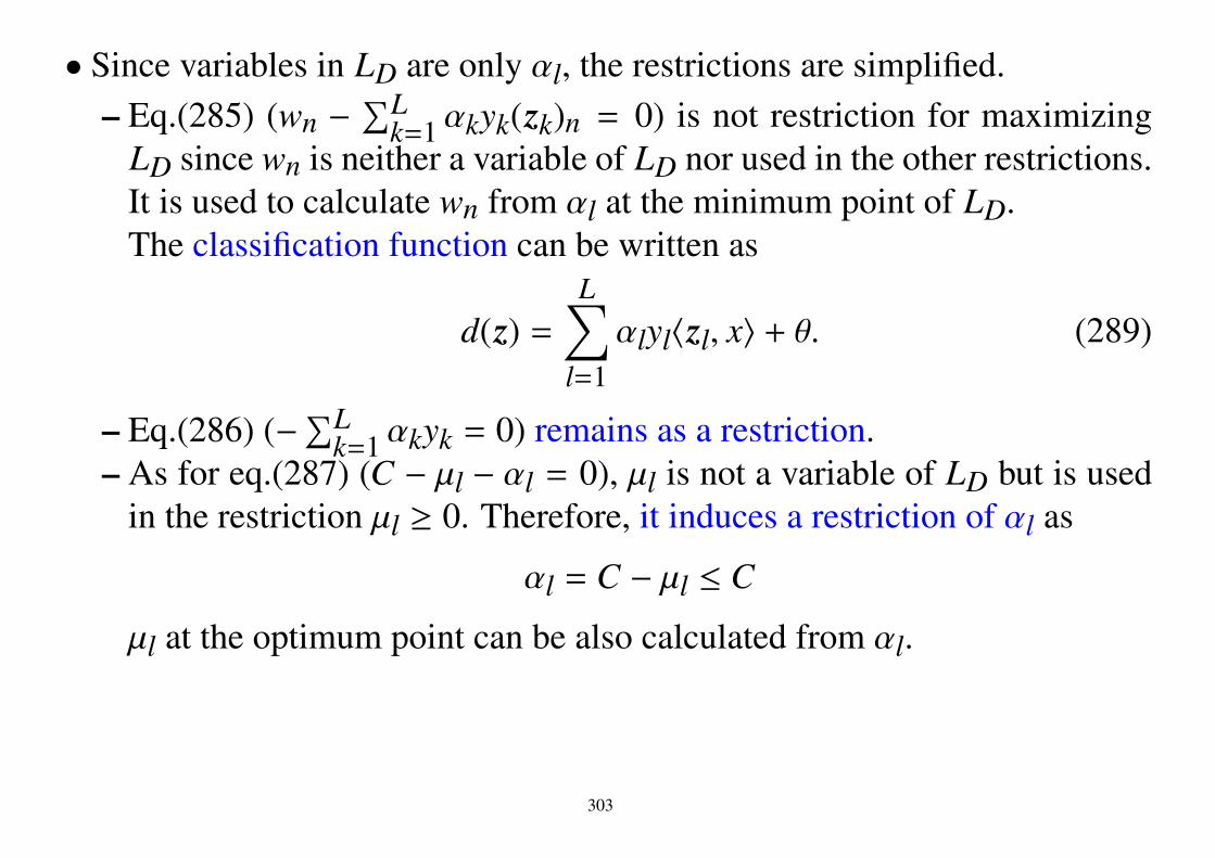
• Since variables in LD are only αl, the restrictions are simplified.– Eq.(285) (wn −
∑Lk=1 αkyk(zk)n = 0) is not restriction for maximizing
LD since wn is neither a variable of LD nor used in the other restrictions.It is used to calculate wn from αl at the minimum point of LD.The classification function can be written as
d(z) =L∑
l=1αlyl⟨zl, x⟩ + θ. (289)
– Eq.(286) (−∑Lk=1 αkyk = 0) remains as a restriction.
– As for eq.(287) (C − µl − αl = 0), µl is not a variable of LD but is usedin the restriction µl ≥ 0. Therefore, it induces a restriction of αl as
αl = C − µl ≤ C
µl at the optimum point can be also calculated from αl.
303

Optimization problem to be solvedSubject to
0 ≤ αl ≤ C,L∑
l=1αlyl = 0 (l = 1, 2, . . . L) (290)
Maximize
LD =L∑lαl −
12
L∑l=1
L∑k=1
αlαkylyk⟨zl, zk⟩ (291)
– Variables for optimization problem are only αl.– The dimension of this problem is the number of samples.– w can be calculated by eq.(285).
w =L∑
k=1αkykzk
– θ is obtained by using KKT condition.
304

• KKT condition of the primal problemFor l = 1, 2, . . . L,
∂LP∂wn= wn −
L∑k=1
αkyk(zk)n = 0 (292)
∂LP∂θ= −
L∑k=1
αkyk = 0 (293)
∂LP∂ξl= C − µl − αl = 0 (294)
yl(⟨w, zl⟩ + θ) − 1 + ξl ≥ 0 (295)ξl ≥ 0 (296)
αl ≥ 0, µl ≥ 0 (297)αlyl(⟨w, zl⟩ + θ) − 1 + ξl = 0 (298)
µlξl = 0 (299)
where wl and (zk)l are the l-th component of w and zk, respectively.
305

KKT conditions imply• 0 < αl < C
– 0 < µl < C yields ξl = 0 and we have yl(⟨w, zl⟩ + θ) − 1 = 0.⇒ zl is on the boundary for the margin.
– Such a point is called the support vector (SV).(Sometimes zl for αl = C is also called SV.)
– θ can be obtained by SVs.
θ = −⟨w, zl⟩ + yl
• αl = 0– µl = C yields ξl = 0 and we have yl(⟨w, zl⟩ + θ) − 1 ≥ 0.⇒ zl is included in the correct half space not in the margin region.
• αl = C– µl = 0 yields ξl ≥ 0 and we have yl(⟨w, xl⟩ + θ) − 1 + ξl = 0.⇒ xl is included in the wrong half space or the margin region.
306

11.6.4 Support Vector Machine (SVM)• SV’ : the set of zl for αl > 0• Classification function:
d(x) =L∑
k=1αkyk⟨zk, x⟩ + θ
=∑
xk∈SV′αkyk⟨zk, x⟩ + θ.
• The sum is not for all training patterns but for SVs⇒ Linear support vector machine• Computational cost of classification is reduced.
307

•We don’t have to calculate the following parameters for obtaining d(x).– µl can be obtained from eq.(294).
µl = C − αl
µl ≥ 0 is satisfied.– ξl can be obtained from eqs.(298).
If αl , C,ξi = 0
If αl = C,ξl = −yl(⟨w, zl⟩ + θ) + 1
• Remark : We cannot substitute eqs.(298), (299) into LP for optimizationproblem since they hold only at a stationary point.
⇒ If we substitute it, derivatives can not be obtained correctly.
308

11.6.5 VC dimension• Recall VC (Vapnik Chervonenkis) dimension.
The maximum number of points that the classifiers can shatter for anylabeling of them.
• The VC dimension of linear classifiers in n-dimensional space is: n + 1.
309

11.6.6 Kernel method• After patterns are mapped by a nonlinear function Φ into a very high (or
infinite) dimensional space, linear classification is performed.
Example: Φ(x1, x2) = (x21, x2
2,√
2x1x2,√
2x1,√
2x2, 1)
310

• However, the cost of calculation in a high or infinite dimensional space byusing Φ(x) is huge.• In many case, only by the inner product
⟨Φ(x),Φ(z)⟩ = k(x, z)
in the space, we can construct a classifier and classify input patterns with-out direct calculation in the space.• For the previous example:
Φ((x1, x2)) = (x21, x
22,√
2x1x2,√
2x1,√
2x2, 1),
its kernel function is given by
k(x, z) = ⟨Φ(x),Φ(z)⟩= x2
1z21 + x2
2z22 + 2x1x2z1z2 + 2x1z1 + 2x2z2 + 1
= (x1z1 + x2z2 + 1)2
= (⟨x, z⟩ + 1)2 .
⇒ Simple.
311

Definition 6. Mercer kernel function is defined as a function satisfying thefollowing condition.
• Symmetric : k(x, z) = k(z, x)• Positive definite : For any function h(z), we have∫ ∫
k(x, z)h(x)h(z)dxdz ≥ 0.
Theorem 17. Let k(x, y) be a Mercer kernel function. Then, there exists amapping Φ(x) such that
⟨Φ(x),Φ(z)⟩ = k(x, z).
312

Kernel method
•When we fix a Mercer kernel function, we can calculate inner productsbetween patterns mapped by Φ without calculating Φ.•Many classifiers do not need Φ(x) but their inner product.•We can extend such classifiers to those of nonlinear version.
Examples of kernel functions :
k(x, y) = ⟨x, y⟩ (Linear kernel) (300)
k(x, y) = (⟨x, y⟩ + 1)20 (Polynomial kernel) (301)
k(x, y) = exp∥x − y∥2/(2σ2) (Gaussian kernel) (302)
313

11.6.7 (nonlinear) SVM• Classification function and its criterion of linear SVM are expressed only
by inner products.⇒ Kernel method can be applied.• Classification function
d(x) =∑
zl∈S Vαlylk(zl, x) + θ (303)
• The optimization problem for learning is given asSubject to
0 ≤ αl ≤ C,L∑
l=1αlyl = 0 (l = 1, 2, . . . L), (304)
minimize
LD =L∑lαl −
12
L∑l=1
L∑k=1
αlαkylykk(zl, zk) (305)
with respect to αl.
314

12 ConclusionRemember
• Eigenvalue problem• SVD• Generalized inverses• Normal distribution• Test• Estimation• Cramer-Rao lower bound, Fisher information matrix• Statistical learning theory• Conjugate gradient method• Quasi-Newton’s method
→ International Development Engineering
315