Embed Size (px)
Citation preview
MATHEMATICS BONUS FILES for faculty and students http://www2.onu.edu/~mcaragiu1/bonus_files.html
RECEIVED: November 1, 2007 PUBLISHED: November 7, 2007
Solving integrals by differentiation with respect to a parameter
Khristo N. Boyadzhiev
Department of Mathematics Ohio Northern University
Ada, OH 45810 [email protected]
Contents.
1. Introduction
2. Examples
3.Using differential equations
4 Advanced technique using the Leibniz Integral Rule
5 Theory
References
1
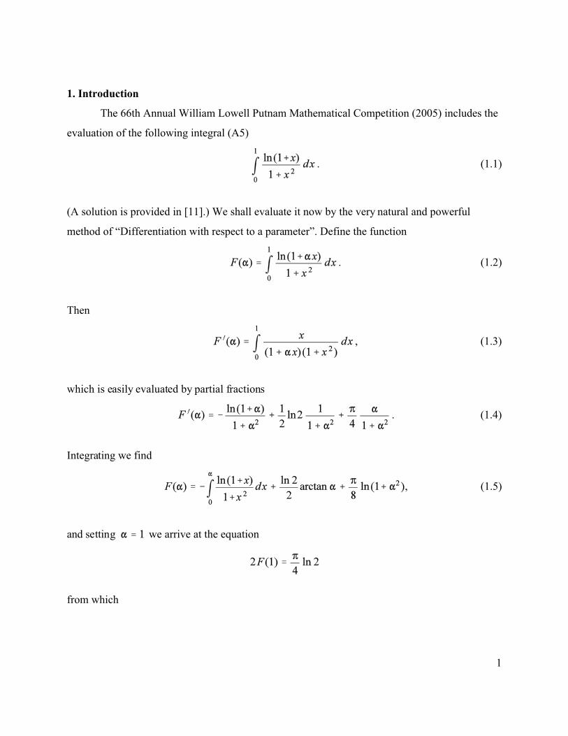
1. Introduction
The 66th Annual William Lowell Putnam Mathematical Competition (2005) includes the
evaluation of the following integral (A5)
. (1.1)
(A solution is provided in [11].) We shall evaluate it now by the very natural and powerful
method of “Differentiation with respect to a parameter”. Define the function
. (1.2)
Then
, (1.3)
which is easily evaluated by partial fractions
. (1.4)
Integrating we find
, (1.5)
and setting we arrive at the equation
from which

2
. (1.6)
This example illustrates the method very well. Many integrals containing “log”, “arctan”,
“arcsin”, can be evaluated this way.
Note. Equation (1.5) can be used to evaluate
, (1.7)
where is Catalan’s constant (see [1]).
(1.8)
In what follows we present several examples involving the “differentiation on a
parameter” method. Some theorems ensuring the legitimacy of the work are listed at the end.
Applying the theorems in every particular case is left to the reader.
Our main reference in the excellent book of Fikhtengolts [5].
2. Examples
Example 2.1
Consider the integral
(2.1.1)
where . Differentiating for we find:
,
3
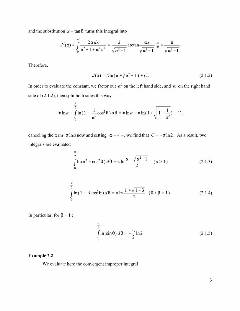
and the substitution turns this integral into
.
Therefore,
. (2.1.2)
In order to evaluate the constant, we factor out on the left hand side, and on the right hand
side of (2.1.2), then split both sides this way
,
canceling the term now and setting , we find that . As a result, two
integrals are evaluated
(2.1.3)
. (2.1.4)
In particular, for :
. (2.1.5)
Example 2.2
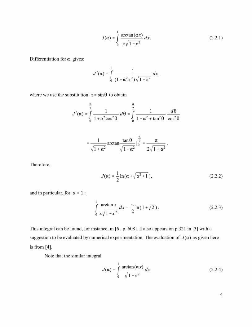
We evaluate here the convergent improper integral
4
. (2.2.1)
Differentiation for gives:
,
where we use the substitution to obtain
.
Therefore,
, (2.2.2)
and in particular, for :
. (2.2.3)
This integral can be found, for instance, in [6 , p. 608]. It also appears on p.321 in [3] with a
suggestion to be evaluated by numerical experimentation. The evaluation of as given here
is from [4].
Note that the similar integral
(2.2.4)
5
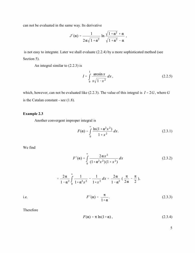
can not be evaluated in the same way. Its derivative
,
is not easy to integrate. Later we shall evaluate (2.2.4) by a more sophisticated method (see
Section 5).
An integral similar to (2.2.3) is
, (2.2.5)
which, however, can not be evaluated like (2.2.3). The value of this integral is , where
is the Catalan constant - see (1.8).
Example 2.3
Another convergent improper integral is
. (2.3.1)
We find
(2.3.2)
,
i.e. . (2.3.3)
Therefore
, (2.3.4)
6
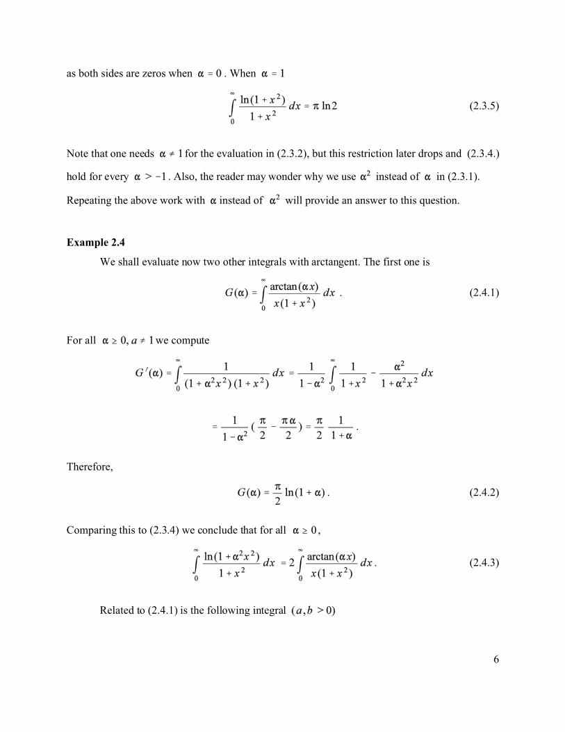
as both sides are zeros when . When
(2.3.5)
Note that one needs for the evaluation in (2.3.2), but this restriction later drops and (2.3.4.)
hold for every . Also, the reader may wonder why we use instead of in (2.3.1).
Repeating the above work with instead of will provide an answer to this question.
Example 2.4
We shall evaluate now two other integrals with arctangent. The first one is
. (2.4.1)
For all we compute
.
Therefore,
. (2.4.2)
Comparing this to (2.3.4) we conclude that for all ,
. (2.4.3)
Related to (2.4.1) is the following integral
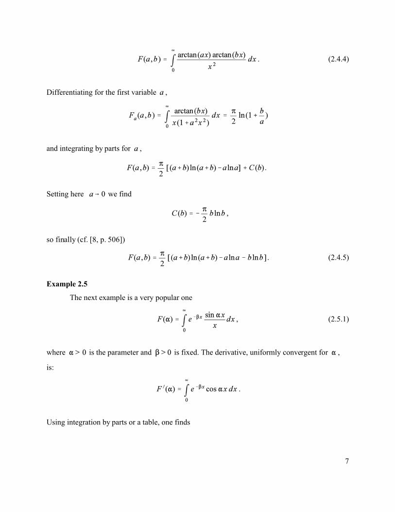
7
. (2.4.4)
Differentiating for the first variable ,
and integrating by parts for ,
.
Setting here we find
,
so finally (cf. [8, p. 506])
. (2.4.5)
Example 2.5
The next example is a very popular one
, (2.5.1)
where is the parameter and is fixed. The derivative, uniformly convergent for ,
is:
.
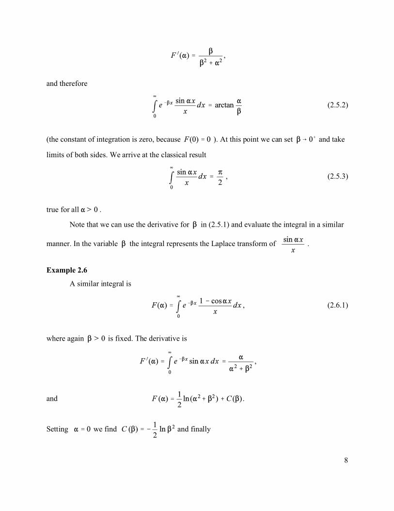
Using integration by parts or a table, one finds
8
,
and therefore
(2.5.2)
(the constant of integration is zero, because ). At this point we can set and take
limits of both sides. We arrive at the classical result
, (2.5.3)
true for all .
Note that we can use the derivative for in (2.5.1) and evaluate the integral in a similar
manner. In the variable the integral represents the Laplace transform of .
Example 2.6
A similar integral is
, (2.6.1)
where again is fixed. The derivative is
,
and .
Setting we find and finally
9
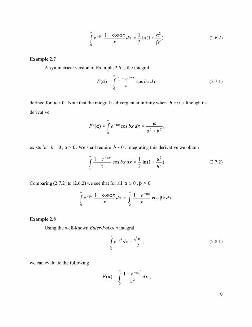
. (2.6.2)
Example 2.7
A symmetrical version of Example 2.6 is the integral
(2.7.1)
defined for . Note that the integral is divergent at infinity when , although its
derivative
,
exists for . We shall require . Integrating this derivative we obtain
. (2.7.2)
Comparing (2.7.2) to (2.6.2) we see that for all
.
Example 2.8
Using the well-known Euler-Poisson integral
, (2.8.1)
we can evaluate the following
,
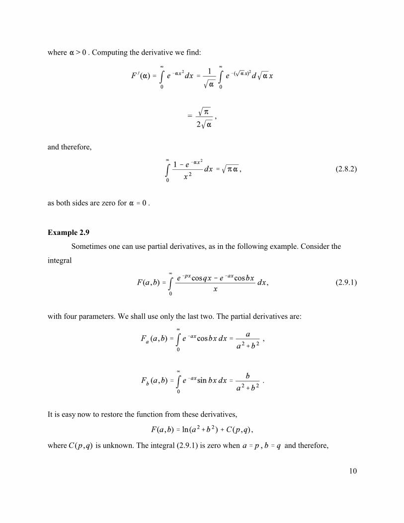
10
where . Computing the derivative we find:
= ,
and therefore,
, (2.8.2)
as both sides are zero for .
Example 2.9
Sometimes one can use partial derivatives, as in the following example. Consider the
integral
, (2.9.1)
with four parameters. We shall use only the last two. The partial derivatives are:
,
.
It is easy now to restore the function from these derivatives,
,
where is unknown. The integral (2.9.1) is zero when and therefore,
11
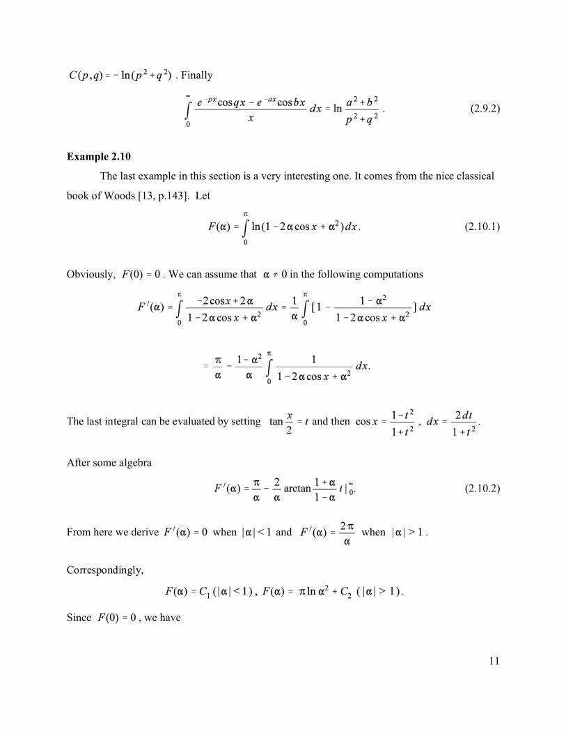
. Finally
. (2.9.2)
Example 2.10
The last example in this section is a very interesting one. It comes from the nice classical
book of Woods [13, p.143]. Let
. (2.10.1)
Obviously, . We can assume that in the following computations
.
The last integral can be evaluated by setting and then , .
After some algebra
. (2.10.2)
From here we derive when and when .
Correspondingly,
.
Since , we have
12
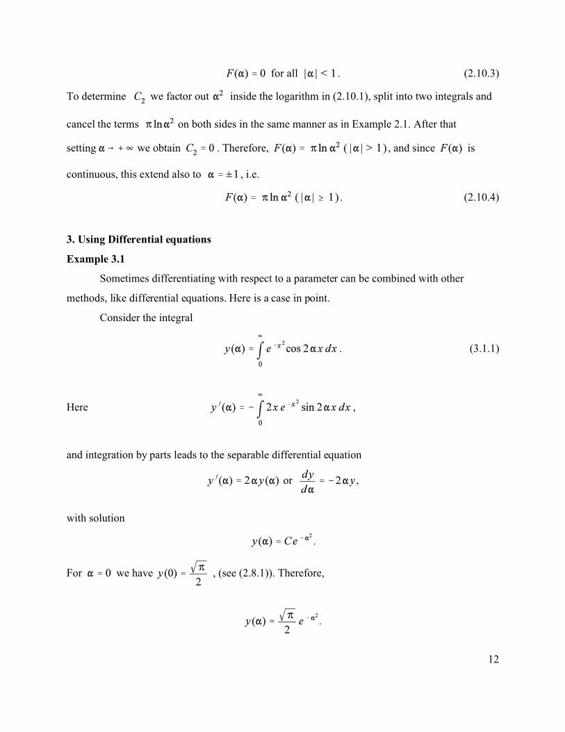
for all . (2.10.3)
To determine we factor out inside the logarithm in (2.10.1), split into two integrals and
cancel the terms on both sides in the same manner as in Example 2.1. After that
setting we obtain . Therefore, , and since is
continuous, this extend also to , i.e.
. (2.10.4)
3. Using Differential equations
Example 3.1
Sometimes differentiating with respect to a parameter can be combined with other
methods, like differential equations. Here is a case in point.
Consider the integral
. (3.1.1)
Here ,
and integration by parts leads to the separable differential equation
or ,
with solution
.
For we have , (see (2.8.1)). Therefore,
.
13
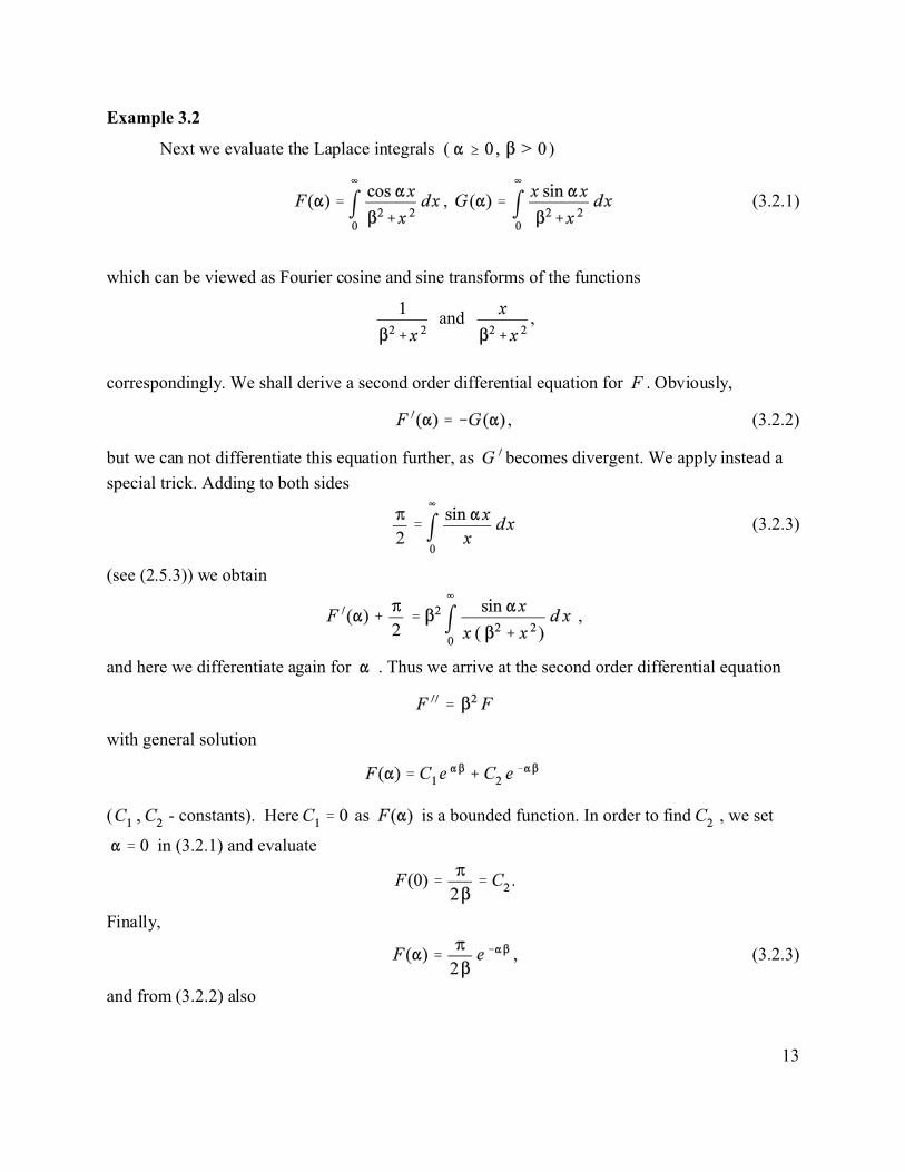
Example 3.2
Next we evaluate the Laplace integrals ( )
, (3.2.1)
which can be viewed as Fourier cosine and sine transforms of the functions
and ,
correspondingly. We shall derive a second order differential equation for . Obviously,
, (3.2.2)
but we can not differentiate this equation further, as becomes divergent. We apply instead a
special trick. Adding to both sides
(3.2.3)
(see (2.5.3)) we obtain
,
and here we differentiate again for . Thus we arrive at the second order differential equation
with general solution
( - constants). Here as is a bounded function. In order to find , we set
in (3.2.1) and evaluate
.
Finally,
, (3.2.3)
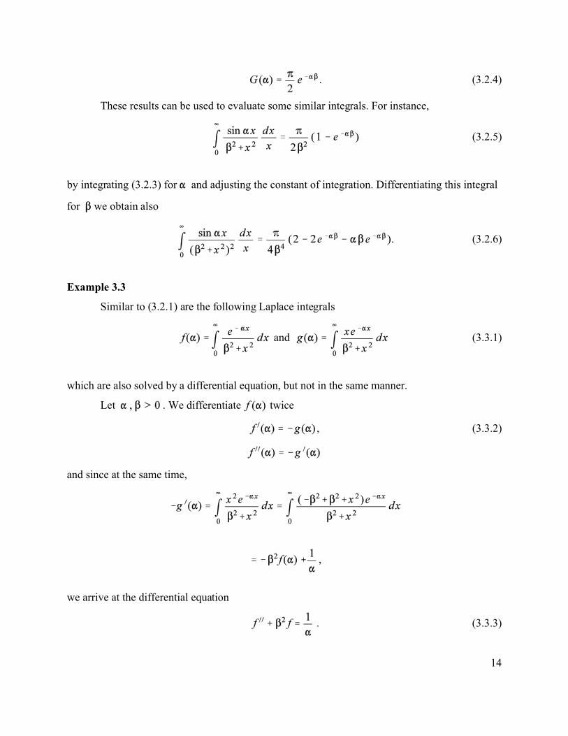
and from (3.2.2) also
14
. (3.2.4)
These results can be used to evaluate some similar integrals. For instance,
(3.2.5)
by integrating (3.2.3) for and adjusting the constant of integration. Differentiating this integral
for we obtain also
. (3.2.6)
Example 3.3
Similar to (3.2.1) are the following Laplace integrals
and (3.3.1)
which are also solved by a differential equation, but not in the same manner.
Let . We differentiate twice
, (3.3.2)
and since at the same time,
,
we arrive at the differential equation
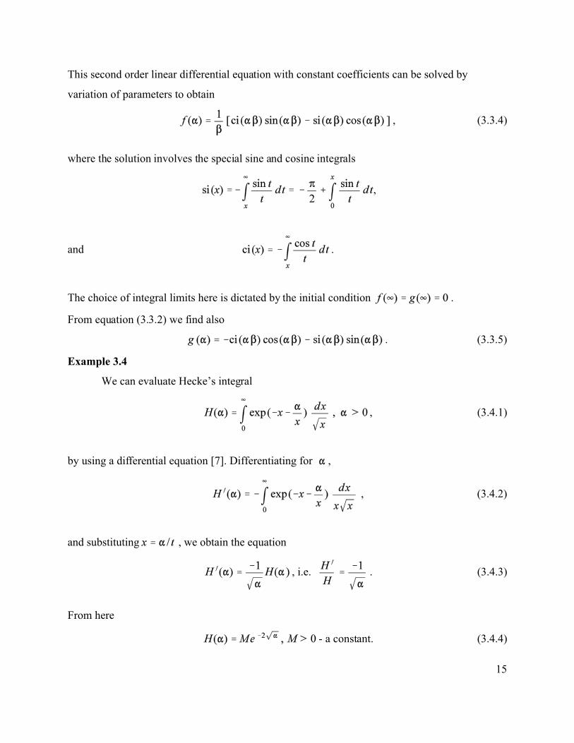
. (3.3.3)
15
This second order linear differential equation with constant coefficients can be solved by
variation of parameters to obtain
, (3.3.4)
where the solution involves the special sine and cosine integrals
,
and .
The choice of integral limits here is dictated by the initial condition .
From equation (3.3.2) we find also
. (3.3.5)
Example 3.4
We can evaluate Hecke’s integral
, (3.4.1)
by using a differential equation [7]. Differentiating for ,
, (3.4.2)
and substituting , we obtain the equation
, i.e. . (3.4.3)
From here
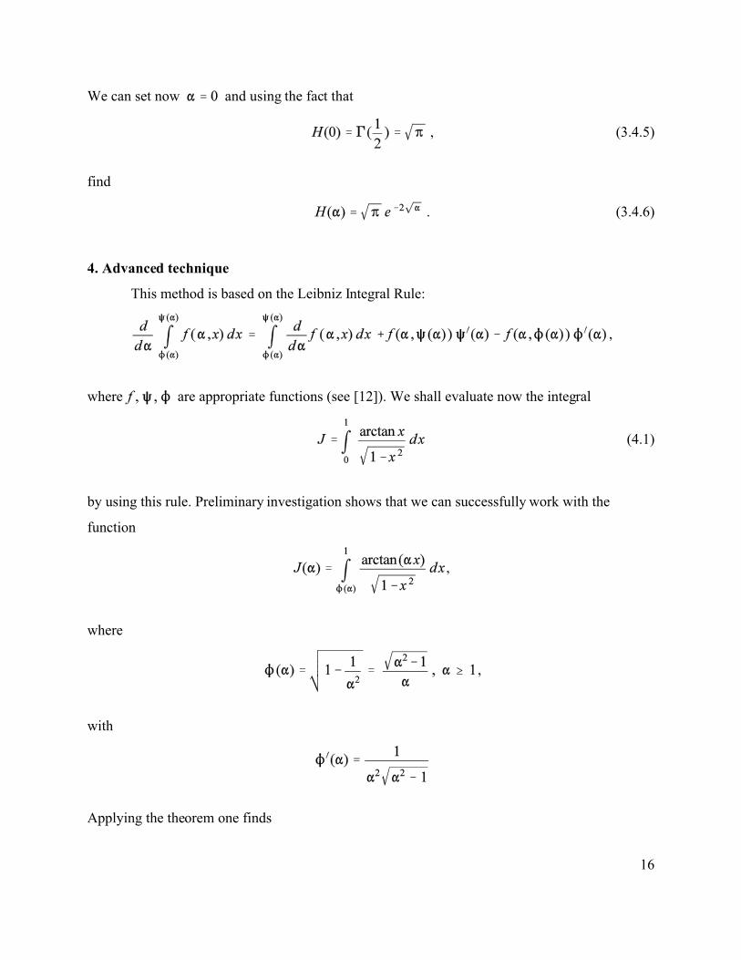
- a constant. (3.4.4)
16
We can set now and using the fact that
, (3.4.5)
find
. (3.4.6)
4. Advanced technique
This method is based on the Leibniz Integral Rule:
,
where are appropriate functions (see [12]). We shall evaluate now the integral
(4.1)
by using this rule. Preliminary investigation shows that we can successfully work with the
function
,
where
,
with
Applying the theorem one finds
17
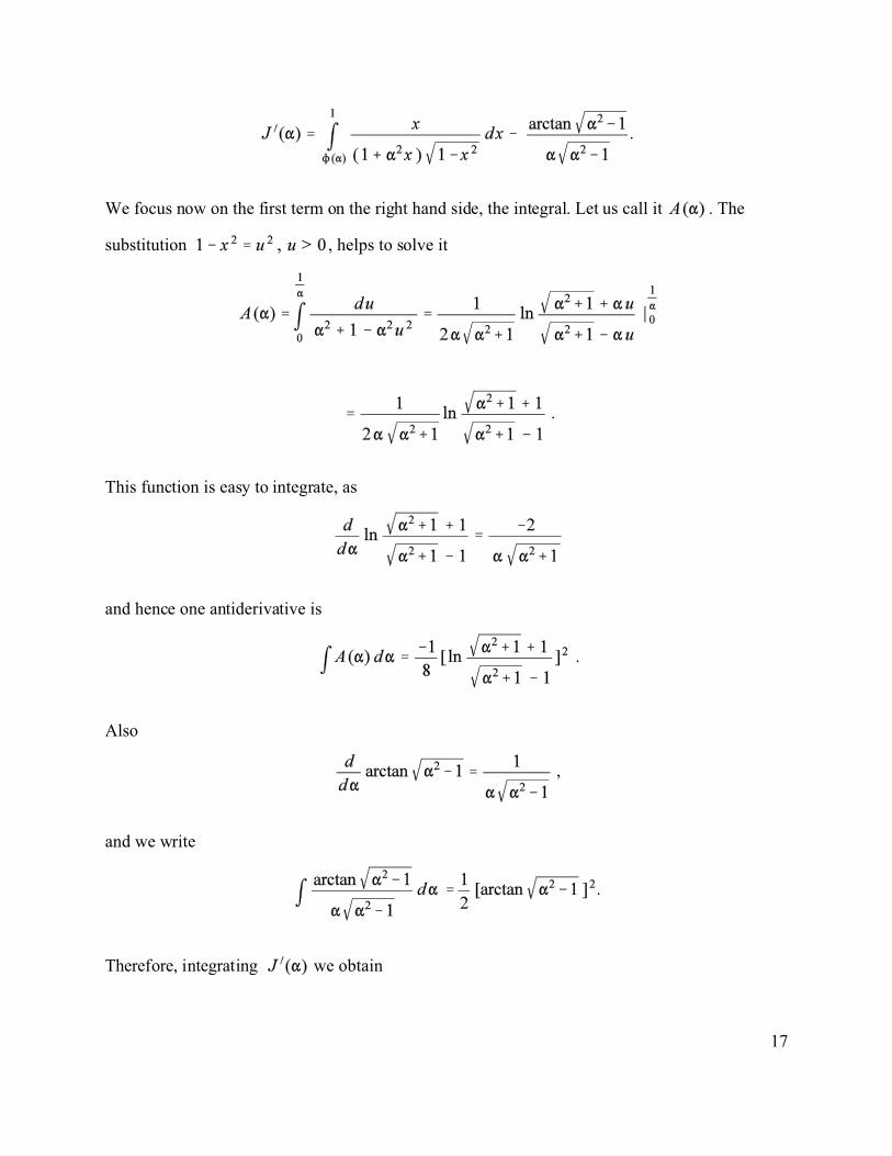
.
We focus now on the first term on the right hand side, the integral. Let us call it . The
substitution , helps to solve it
.
This function is easy to integrate, as
and hence one antiderivative is
.
Also
,
and we write
.
Therefore, integrating we obtain
18
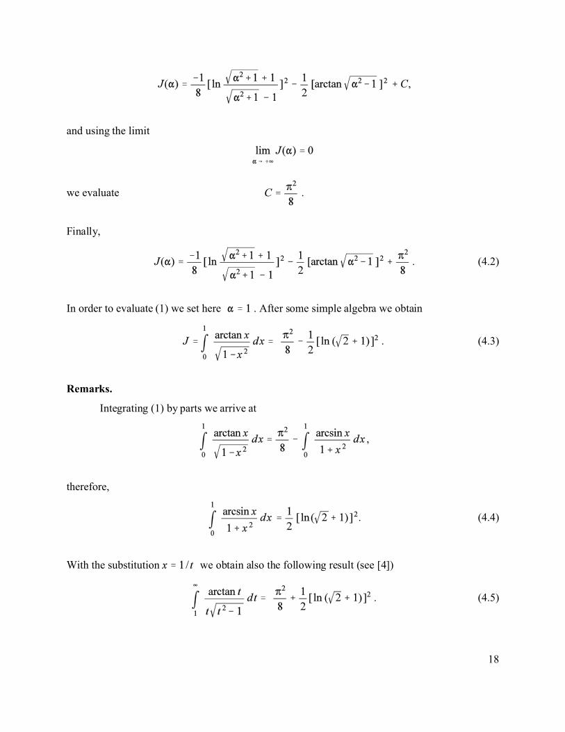
,
and using the limit
we evaluate .
Finally,
. (4.2)
In order to evaluate (1) we set here . After some simple algebra we obtain
. (4.3)
Remarks.
Integrating (1) by parts we arrive at
,
therefore,
. (4.4)
With the substitution we obtain also the following result (see [4])
. (4.5)
19
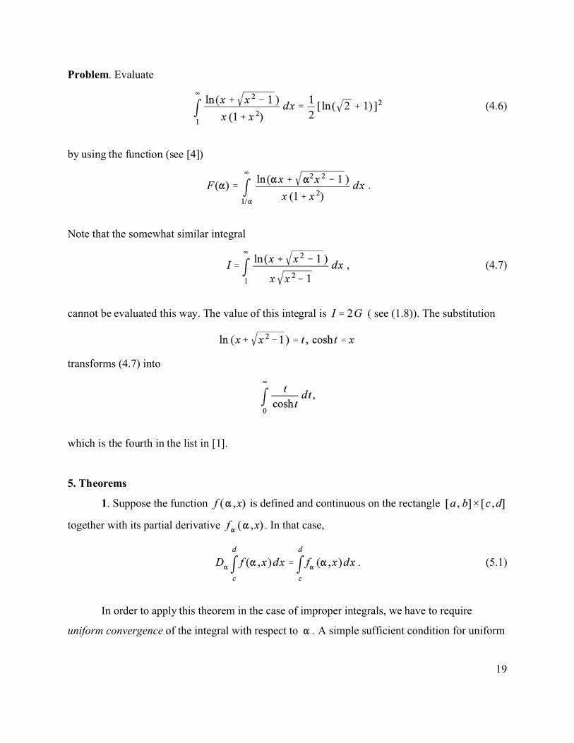
Problem. Evaluate
(4.6)
by using the function (see [4])
.
Note that the somewhat similar integral
, (4.7)
cannot be evaluated this way. The value of this integral is ( see (1.8)). The substitution
transforms (4.7) into
,
which is the fourth in the list in [1].
5. Theorems
1. Suppose the function is defined and continuous on the rectangle
together with its partial derivative . In that case,
. (5.1)
In order to apply this theorem in the case of improper integrals, we have to require
uniform convergence of the integral with respect to . A simple sufficient condition for uniform
20
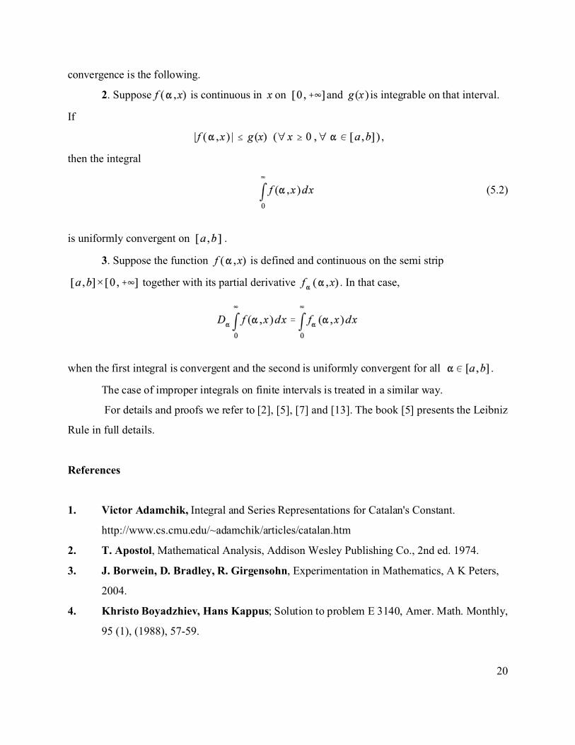
convergence is the following.
2. Suppose is continuous in on and is integrable on that interval.
If
,
then the integral
(5.2)
is uniformly convergent on .
3. Suppose the function is defined and continuous on the semi strip
together with its partial derivative . In that case,
when the first integral is convergent and the second is uniformly convergent for all .
The case of improper integrals on finite intervals is treated in a similar way.
For details and proofs we refer to [2], [5], [7] and [13]. The book [5] presents the Leibniz
Rule in full details.
References
1. Victor Adamchik, Integral and Series Representations for Catalan's Constant.
http://www.cs.cmu.edu/~adamchik/articles/catalan.htm
2. T. Apostol, Mathematical Analysis, Addison Wesley Publishing Co., 2nd ed. 1974.
3. J. Borwein, D. Bradley, R. Girgensohn, Experimentation in Mathematics, A K Peters,
2004.
4. Khristo Boyadzhiev, Hans Kappus; Solution to problem E 3140, Amer. Math. Monthly,
95 (1), (1988), 57-59.
21
5. G. M. Fikhtengolts, A Course of differential and integral calculus (Russian), Vol 2,
Nauka, Moscow 1066.
6. I. S. Gradshteyn and I. M. Ryzhik, Tables of Integrals, Series, and Products, Academic
Press, 1980.
7. Omar Hijab, Introduction to Calculus and Classical Analysis, Springer, 1997.
8. A. P. Prudnikov, Yu. A. Brychkov, O. I. Marichev, Integrals and Series, Vol.1:
Elementary Functions, Gordon and Breach 1986.
9. Joseph Wiener, Differentiation with respect to a parameter, College Mathematics
Journal, 32, No. 3.(2001), pp. 180-184.
10. Joseph Wiener, Donald P. Skow, Differentiating indefinite integrals with respect to a
parameter. Missouri Journal of Mathematical Sciences, Vol. 3, no 2, (1991), 65-69.
11. 66th Annual William Lowell Putnam Mathematical Competition, Math. Magazine,
79 (2006), 76-79.
12. Eric W. Weisstein. "Leibniz Integral Rule." From MathWorld--A Wolfram Web
Resource. http://mathworld.wolfram.com/LeibnizIntegralRule.html
13. Woods, F. S. Advanced Calculus. New Edition. A Course Arranged with Special
Reference to the Needs of Students of Applied Mathematics. Ginn and Co., Boston, MA:
Ginn, Boston, 1954.
Updated November 2007