Mathematics for Graphics and Vision

Steven Mills

March 3, 2016

Contents

1 Introduction 5

2 Scalars 62.1 Visualising Scalars . . . . . . . . . . . . . . . . . . . . . . . . 62.2 Operations on Scalars . . . . . . . . . . . . . . . . . . . . . . 62.3 A Note on Multiplication Symbols . . . . . . . . . . . . . . . 7

3 Trigonometric Functions 83.1 Degrees and Radians . . . . . . . . . . . . . . . . . . . . . . . 93.2 Sine, Cosine, and Tangent . . . . . . . . . . . . . . . . . . . . 93.3 Plots of Trigonometric Functions . . . . . . . . . . . . . . . . 103.4 Inverse Functions . . . . . . . . . . . . . . . . . . . . . . . . . 103.5 Some Common Angles . . . . . . . . . . . . . . . . . . . . . . 11

4 Vectors 134.1 Visualising Vectors . . . . . . . . . . . . . . . . . . . . . . . . 134.2 Some Special Vectors . . . . . . . . . . . . . . . . . . . . . . . 134.3 Vector Addition and Subtraction . . . . . . . . . . . . . . . . 144.4 Scalar Multiplication . . . . . . . . . . . . . . . . . . . . . . . 154.5 The Dot Product . . . . . . . . . . . . . . . . . . . . . . . . . 164.6 Vector Lengths and Normalisation . . . . . . . . . . . . . . . 164.7 Vector Cross Product . . . . . . . . . . . . . . . . . . . . . . 174.8 Geometric Interpretation of Products of Vector . . . . . . . . 17

5 Matrices 195.1 Matrix Addition and Subtraction . . . . . . . . . . . . . . . . 195.2 Scalar Multiplication . . . . . . . . . . . . . . . . . . . . . . . 215.3 Matrix Multiplication . . . . . . . . . . . . . . . . . . . . . . 21

1

5.4 Matrix Transpose . . . . . . . . . . . . . . . . . . . . . . . . . 225.5 Matrices as Transforms of Vectors . . . . . . . . . . . . . . . 235.6 The Identity Matrix . . . . . . . . . . . . . . . . . . . . . . . 245.7 Inverse Matrices . . . . . . . . . . . . . . . . . . . . . . . . . 24

2

Notation Summary

General Notation

a, b, . . . Lower case letters in italics are scalars (simple numbers)a,b, . . . Lower case letters in bold are vectors (1-D arrays of numbers)A,B, . . . Upper case letters are matrices (2-D arrays of numbers)sin2(θ) Means (sin(θ))2, not sin(sin(θ)). Similarly for cos and tan.sin−1(x) Arcsine, the angle whose sine is x. Similarly for cos and tan.

Matrices and Vectors

vi The ith element of a vector, vmij The element of a matrix, M, in the ith row and jth columnvT,MT Transpose of a vector or matrix

0 The zero-vector, 0 =[0 0 . . . 0

]T.

u · v Dot product (a scalar value) of two vectorsu× v Cross product (a 3-vector) of two 3-vectors‖v‖ The length of a vector, ‖v‖ =

√v · v

v A unit vector in the same direction as v, v = v‖v‖ .

u ⊥ v The vectors u and v are perpendicular to one another.u ‖ v The vectors u and v are parallel to one another.I The identity matrix, with diagonal entries of 1, and off-

diagonal entries of 0.M−1 The inverse of a matrix, M. MM−1 = I = M−1M.

3

Quick Reference

A few results and identities are gathered here for easy reference:

• Trigonometric functions of some common angles:

θ 0 π6

π4

π3

π2

Degrees 0◦ 30◦ 45◦ 60◦ 90◦

Opposite 0 12

1√2

√3

2 1

Adjacent 1√

32

1√2

12 0

Hypotenuse 1 1 1 1 1

sin θ 0 12

1√2

√3

2 1

cos θ 1√

32

1√2

12 0

tan θ 0 1√3

1√

3 –

• sin2(θ) + cos2(θ) = 1.

• The angle between two vectors is cos−1(

u·v‖u‖‖v‖

).

• Two non-zero vectors are perpendicular if and only if u · v = 0.

• Two unit vectors are parallel if and only if u · v = 1.

• Two non-zero 3-vectors are parallel if and only if u× v = 0.

• u× v is perpendicular to u and v unless they are zero or parallel.

• Matrix multiplication is not commutative, so AB 6= BA in general.

• Inverses and transposes of products reverse the order of multiplication,so (AB)T = BTAT and (AB)−1 = B−1A−1.

4

1 Introduction

This document provides mathematics which is be useful for computer graph-ics and vision students. It is mainly aimed at students taking COSC342(Computer Graphics) at Otago, but may be of interest to those takingrelated papers such as COSC360 (Computer Game Design) or COSC450(Computer Graphics and Vision) as well.

We will be dealing with three main types of mathematical object –scalars, vectors, and matrices. Scalars are just ordinary numbers like 1,−23

7 , or π. Vectors are one-dimensional arrays of numbers, and matricesare two-dimensional arrays of numbers. It is important to keep the type ofvalues in mind, because it affects what you can do with them and what theresult is. For example, while it makes sense to divide two numbers (as longas the second is not zero), division is not defined for vectors or matrices.

Vectors will be used to represent geometric objects like points and lines.Matrices will represent transformations of these objects, like scaling, trans-lation, and rotation. Using vector and matrix notation gives us a set ofoperations (an algebra) to work with. Representing these geometric ideasalgebraically is very useful, since it allow us to easily write computer pro-grams that work with them.

5

2 Scalars

We’ll start by revising some properties of scalars (ordinary numbers). Thismay be familiar to you, but it is important to make sure we have a commonlanguage and have defined a few important terms.

2.1 Visualising Scalars

Scalar values can be visualised on the number line, as shown in Figure 1.

0 2-1-2½ π

Figure 1: The values −212 , −2, 0, 2, and π shown on the number line

Scalars can be thought of as either a point on the line, or as a distancealong the line from zero. If thought of as distances, negative numbers are astep to the left, and positive numbers to the right. Addition can be thoughtof as combining steps, and multiplication as repeating a step. So 2− 3 is astep of 2 units to the right, followed by a step of 3 units to the left. Instead2×3 can be thought of as taking two steps to the right three times (although6 is not shown in Figure 1).

2.2 Operations on Scalars

The usual operations that are applied to numbers are addition, subtrac-tion, multiplication, and division. For this discussion, it helps to think ofsubtraction as adding negative numbers, and as division as multiplying byreciprocals, so when we see 1− 3, we think 1 + (−3), and by 1÷ 2 we mean1 × 1

2 . This makes the order of operations easier, because the meaning of1−2+3, is not immediately clear – is it 1−(2+3) = −4 or (1−2)+3 = 2? Ifwe think of this as 1 + (−2) + 3 then the order of operations doesn’t matter.Likewise 1÷ 3× 2 is not clear, but 1× 1

3 × 2 is.This leads us to the first properties of addition and multiplication – they

are associative and commutative, which means that when you add a list ofnumbers or multiply a list of numbers the order in which do you thingsdoesn’t matter.

More formally the commutative rule for addition says that

a+ b = b+ a ∀a, b. (1)

6

A few words about notation are probably useful here. Firstly, we use lowercase italic letters to denote scalars. Secondly, the symbol ∀, which is usu-ally read ‘for all’, means that this is true for any values of a and b. Thecommutative rule for multiplication tells us that

a× b = b× a ∀a, b. (2)

The associative rule tells us that we can apply multiple instances ofaddition or multiplication in any order. For addition this gives us

a+ (b+ c) = (a+ b) + c ∀a, b, c, (3)

and for multiplication

a× (b× c) = (a× b)× c ∀a, b, c. (4)

Things get a little more complex when we mix multiplication and addi-tion, but the key rule is to apply multiplication first, unless brackets tell youotherwise. So 1 + 2× 3 means 1 + (2× 3), and 1× 2 + 3 means (1× 2) + 3.Combining operators also gives us a third property – distributive. We saythat multiplication distributes over addition to mean that

a× (b+ c) = (a× b) + (a× c) ∀a, b, c. (5)

Note that addition does not distribute over multiplication, since

1 + (2× 3) 6= (1 + 2)× (1 + 3). (6)

2.3 A Note on Multiplication Symbols

There are many ways to write multiplication of two values. The most usualis form is probably a × b, which we’ve used so far, but there are two othercommon forms used when dealing with symbols (rather than numbers). Thefirst is a dot, a · b and the second is just writing two symbols side-by-side,ab. Note that when dealing with actual numbers, × is preferred, since 1 · 2can look like 1.2, and 12 is a different number all together. This will becomeimportant when we come to vectors and matrices where multiplication is alittle more complicated.

We’ll typically just place symbols side by side to indicate multiplication,but use × when needed for clarity. Note that this is also why mathematicstypically uses single-letter variables, and why precise notation is important.For example, sin should be read as s× i×n, where as sin is the trigonomet-ric function ‘sine’. (Shortening ‘sine’ to sin doesn’t save much space, butmathematicians do this to make the abbreviation the same length as theshortening of ‘cosine’ to cos and ‘tangent’ to tan.)

7

3 Trigonometric Functions

We will be dealing with angles quite a lot, and this leads to trigonometry.We will need to be familiar with measuring angles in degrees and radians,and with the basic trigonometric functions, sine, cosine, and tangent.

Trigonometry is often introduced in terms of right-angled triangles, butit is also helpful to keep in mind the relationship with circles. These rela-tionships are illustrated in Figure 2.

x

y1θ

s

Figure 2: Angles can be thought about as rotation around a circle, or aspart of a right-angled triangle.

Some points to note from the figure:

• The angle of interest is θ. We will often use Greek letters for angles,but this is just convention, and not always followed.

• We have a unit circle (a circle with radius 1), and measure the angleanti-clockwise from the positive x-axis (the positive x-axis is pointingto the right in Figure 2).

• The angle then relates to some point (x, y) on the circle.

• The length of the arc around the circle to (x, y) is s.

• This point defines a right-angled triangle with sides x, y, and 1.

• The length of the longest side (the hypotenuse) of the triangle is 1.

• The length of the side of the triangle opposite the angle is y.

• The length of the shorter side adjacent the angle is x.

For angles greater than 90◦ this still holds, but the x and/or y valuesmay be negative.

8

3.1 Degrees and Radians

Angles are commonly measured in degrees, but mathematically it is easierto work in radians. Radians measure the distance around a circumferenceof circle of unit radius (r = 1) associated with a given angle, labelled sin Figure 2. Since the total circumference of a unit circle is 2π, that isequivalent to 360◦, and the conversion from an angle, s, measured in radiansto and from the equivalent value, d, in degrees are

s =π

180◦d, d =

180◦

πs. (7)

Note that radians are a unitless quantity – you do not have ‘degreesradian’, and while we may talk about an angle being ‘π2 radians’ for clarity,it is equally correct to just say that the angle is π

2 .

3.2 Sine, Cosine, and Tangent

The trigonometric functions we will use are sine, cosine, and tangent. Theseare denoted sin, cos, and tan. If we think of things in terms of a right-angledtriangle, then

sin θ =O

H, cos θ =

A

H, tan θ =

O

A, (8)

where H is the length of the longest side of the triangle (the hypotenuse), Ois the length of the side opposite the angle, and A is the length of the sideadjacent to the angle. I learned this as SOH CAH TOA, but why a stringon nonsense syllables helps, I don’t know.

If we return to the view of a unit circle, and Figure 2, then we cansubstitute H = 1, O = y, and A = x, giving

sin θ = y, cos θ = x, tan θ =y

x. (9)

For a more general circle, with a radius of r, this can be rearranged to showthat

(x, y) = (r cos θ, r sin θ), (10)

for any point, (x, y) on a circle. The combination of these definitions withPythagoras’ theorem (i.e., a2 +b2 = c2, for a right angled triangle with sidesof length a, b, and hypotenuse c) leads directly to the identity

sin2 θ + cos2 θ = 1, (11)

where the conventional notation is that sin2 θ = (sin θ)2, etc.

9

3.3 Plots of Trigonometric Functions

Plots of the sine and cosine functions are shown in Figure 3. Note that bothfunctions are periodic, so sin(θ + 2π) = sin θ. Also, cos(θ) = sin(θ + π

2 ).

−1

−0.5

0

0.5

1

−3 −2 −1 0 1 2 3 4 5 6

sin(x)cos(x)

Figure 3: Plot of sine and cosine functions.

Figure 4 shows the tangent function. Like sine and cosine it is periodic,with a period of 2π. Note also that tan(θ) is undefined at π

2 , and therefore

at (2k+1)π2 for any integer, k. This comes about directly from the definition

in Equation 8, since the length of the ‘side’ adjacent to the angle is 0. It isimportant to remember that tan(θ) is undefined at these points, not ‘infinite’– the function diverges so it gets larger (more positive) without bound fromone side and smaller (more negative) from the other.

3.4 Inverse Functions

When working with lines and vectors, we often end up computing the sine orcosine of an angle. In some cases we need to find the angle from these values,and so the inverse functions are needed. These are written as sin−1(x), etc.which means ‘the angle which has a sine of x’.

This notation is a little unfortunate, since it conflicts a bit with the ideaof sin2(θ) being (sin(θ))2. Following that logic, sin−1(x) could be interpretedas (sin(θ))−1 = 1

sin(θ) . This is not the usual convention, however.The inverse functions are often referred to as the arcsine, arccosine, and

arctangent. This is why the corresponding functions in languages like C are

10

−4

−2

0

2

4

−3 −2 −1 0 1 2 3 4 5 6

tan(x)

Figure 4: Plot of the tangent functions.

called asin, acos, and atan.Note that the inverse is not unique, since the trigonometric functions

are periodic. Furthermore, there are generally two angles in each cycle withthe same value for each function. For example, cos(−θ) = cos(θ) for anyθ. By convention, cos−1(x) is treated as the value in the range [0, π], whilesin−1(x) and tan−1(x) return a value in the range [−π

2 ,π2 ].

3.5 Some Common Angles

While in computation we will generally use any value for angles, comput-ing trigonometric functions for an arbitrary angle by hand is not generallyrecommended. However, for a set of common angles, the trigonometricfunctions can be easily expressed. These arise from two special right-angledtriangles – one with two 45◦ angles, and one with a 30◦ and 60◦ angles.

The 45◦–45◦–90◦ triangle has two equal sides, and the longest side has alength of 1. Pythagoras’ theorem tells us that if the length of the other twosides is a, then a2 + a2 = 1, so a = 1√

2.

The 30◦–60◦–90◦ triangle is half of an equilateral triangle with sides oflength 1. This means that the shortest side (adjacent to the 60◦ angle) haslength 1

2 . Therefore the remaining side length, b is found from(1

2

)2

+ b2 = 1, (12)

11

which tells us that b =√

32 .

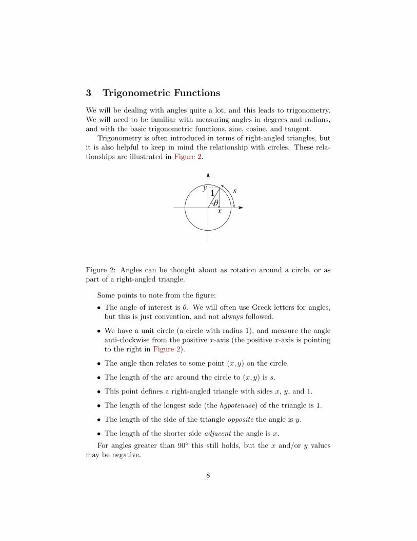
These results, and the trigonometric functions that follow directly fromthem are summarised in Table 1.

θ 0 π6

π4

π3

π2

Degrees 0◦ 30◦ 45◦ 60◦ 90◦

Opposite 0 12

1√2

√3

2 1

Adjacent 1√

32

1√2

12 0

Hypotenuse 1 1 1 1 1

sin θ 0 12

1√2

√3

2 1

cos θ 1√

32

1√2

12 0

tan θ 0 1√3

1√

3 –

Table 1: Trigonometric function values for some common angles. Note thattan π

2 is undefined.

12

4 Vectors

A vector is a one-dimensional array of numbers, and we write them in boldface, such as v to distinguish them from scalars. Other notations you mightsee for vectors include an arrow or bar over or above a value, such as −→v , v,or v

¯. These alternative notations are often used when writing by hand.

A vector, being an array, has a size, which is the number of elements itcontains. A vector with n elements is called an n-vector, so we talk about2-vectors, 3-vectors, and so on. Note that the size of a vector refers to thenumber of elements in a vector, not how big or small the elements are. Byconvention, the ith element of a vector v is denoted vi, using the same letteror symbol as the vector, but as a scalar.

Vectors may be written out in a number of different ways, and we willfollow the common convention of using column vectors, where the elementsare arranged vertically,

v =

v1

v2...vn

. (13)

This convention will be useful when we come to combine matrices andvectors, but takes up a lot of room on the page. When writing vectorsin text, it is convenient to convert them to rows. The transpose operatorconverts a column vector to a row, or vice-versa, and so we can write vT =[v1 v2 . . . vn

], or equivalently v =

[v1 v2 . . . vn

]T. The transpose is a

matrix operation, and so will be discussed later, but other notations youmight see are a prime, v′, or an asterisk, v∗.

4.1 Visualising Vectors

Just as scalars can be thought of as points or steps along a line, vectors canbe thought of as points or steps in the plane (for 2-vectors), 3D space (for3-vectors) and so on. Some 2-vectors are shown in Figure 5, and can bethought of as either steps along the x- and y-axes, or as points in 2D space.Likewise, a 3-vector can be thought of as steps along the x-, y-, and z-axesin 3D space.

4.2 Some Special Vectors

A few special cases of vectors arise, and lead to some additional notation.The first is a vector where every element is zero. This is called a zero vector,

13

(1,3)

(3,1)

(2½, -1½)

(-2,-2)

(-3,2)

(-2,0) X

Y

Figure 5: Some 2-vectors visualised in the plane. The vector v =[x y

]Tis seen as either the point (x, y), or the step from the origin to (x, y).

and often written 0. There is a whole family of zero vectors of differentlength so we have the zero 2-vector, the zero 3-vector, etc. When the sizeof the vector is clear from context, we’ll just talk about the zero vector.

You might also see 1 for a vector of all ones, but this is less common.Note that 1 is not called the ‘one-vector’. A 1-vector is a vector with oneelement, and is equivalent to a scalar.

4.3 Vector Addition and Subtraction

Vector addition and subtraction are defined simply by adding the corre-sponding elements of a vector, so[

12

]+

[34

]=

[1 + 32 + 4

]=

[46

]. (14)

This only makes sense if there are the same number of elements in eachvector. If the two vectors have different sizes, then their sum is undefined.

14

More generally, the sum of two n-vectors, u and v, is

u + v =

u1

u2...un

+

v1

v2...vn

=

u1 + v1

u2 + v2...

un + vn

. (15)

The difference of two vectors is defined in a similar way,

u− v =

u1

u2...un

−v1

v2...vn

=

u1 − v1

u2 − v2...

un − vn

. (16)

As with scalars, it is sometimes convenient to think of subtraction as adding

a negative, so u− v = u + (−v), where −v =[−v1 −v2 . . . −vn

]T.

The definitions of addition and subtraction can be represented morecompactly if we think about the individual elements. If w = u + v, we cansee that wi = ui + vi. Likewise if d = u− v, then di = ui − vi.

Vector addition has the same properties as scalar addition. Vector addi-tion is commutative and associative, so

u + v = v + u ∀u,v, (17)

andu + (v + w) = (u + v) + w ∀u,v,w. (18)

4.4 Scalar Multiplication

Multiplication of vectors is more complex than for scalars, and there areseveral different types of product that can be formed. The first, and simplest,is scalar multiplication, which is the result of multiplying a vector by a scalar.Like vector addition, this is done element-wise, so multiplying a vector by2 simply doubles each element. More formally, given a scalar, s, and ann-vector, v, their scalar product, u = sv is also an n-vector, with elementsui = s× vi.

Scalar multipliers are conventionally written on the left of the vector,but this is not essential, and vs = sv. Multiplication by several scalarsis associative and commutative, so stv = tsv and s(tv) = (st)v. Finally,multiplication by 0 yields a zero vector of the same size as the original vector,0v = 0.

15

4.5 The Dot Product

The most common form of multiplication with vectors is the dot product,written u ·v. This is also called the scalar product (not to be confused withscalar multiplication) or sometimes the inner product.

Given two vectors of the same size, their dot product is a scalar value.The corresponding elements of the two vectors are multiplied together, andthese are added up to give the result.

More formally,

u · v =

u1

u2...un

·v1

v2...vn

= u1v1 + u2v2 + · · ·+ unvn, (19)

which can be written more compactly as

u · v =

n∑i=1

uivi. (20)

The dot product is commutative, so u · v = v · u. It is not associative,because the dot product of three vectors is undefined. Taking the dot prod-uct of two vectors gives a scalar result, and the dot product of a scalar anda vector is not defined.

The dot product is distributive over vector addition, so

u · (v + w) = u · v + u ·w ∀u,v,w. (21)

Scalar multiplication also factors out, so (ru) · (sv) = rs(u · v).

4.6 Vector Lengths and Normalisation

The length of a vector is written ‖v‖, or |v|, and can be computed as

‖v‖ =√v2

1 + v22 + · · ·+ v2

n =√v · v. (22)

The length of the vector is also called its magnitude or norm, or more pre-cisely its Euclidean norm or 2-norm.

A unit vector is a vector with length 1. Any vector can be converted intoa unit vector by dividing by its length, and we use a ‘hat’ over a vector todenote this,

v =v

‖v‖. (23)

This process is called normalisation.

16

4.7 Vector Cross Product

The final form of multiplication we need for vectors is the cross product.The cross product is only defined for 3-vectors. Given two 3-vectors, u andv, their cross product is also a 3-vector given by

u× v =

u1

u2

u3

×v1

v2

v3

=

u2v3 − u3v2

u3v1 − u1v3

u1v2 − u2v1

(24)

It can be easily shown from this definition that v × v = 0 for any 3-vector,v.

The cross product is not associative, so (u × v) ×w 6= v × (u ×w) ingeneral. The cross product is anticommutative. This means that changingthe order of the vectors does change the result, but in a predictable way,since u× v = −(v × u).

The cross product distributes over addition, so u× (v +w) = uv +uw.Scalar multiplication also interacts in the expected manner so (ru)× (sv) =rs(u× v).

4.8 Geometric Interpretation of Products of Vector

The various products of two vectors have useful geometric interpretations.These are related to the angle between the vectors, and we introduce somenotation for special cases. If two vectors are at right angles to each other,they are perpendicular and we write u ⊥ v. If two vectors point in the samedirection, they are parallel, and we write u ‖ v. The zero-vector, 0, is notparallel or perpendicular to any vector, and is a special case in all of thediscussions that follow.

Two (non-zero) vectors are parallel if, and only if, one is a scalar productof the other. So if u ‖ v, then u = sv for some non-zero s, and vice versa.

The dot product tells us about the angle between vectors, since

u · v = ‖u‖‖v‖ cos θ, (25)

where θ is the angle between the two vectors. If we normalise the vectors,this simplifies to

u · v = cos θ. (26)

Since cos θ = 0 at ±π2 , this means that if the dot product of two non-zero

vectors is 0 if, and only if, they are perpendicular to one another (or one ofthem is 0).

17

In general, the cross product of two vectors is perpendicular to both ofthem, so u ⊥ (u × v), and v ⊥ (u × v). There are two exceptions to thisrule. Firstly, if either vector is 0, then their cross product is 0. This followsdirectly from the definition of the cross product (Equation 24). The secondis if the two vectors are parallel, in this case u = sv, and it follows fairlydirectly that u× v = 0.

These facts help us to solve some common problems that come up incomputer graphics, so to summarise, given two non-zero vectors u and v:

• The angle between the vectors is cos−1(

u·v‖u‖‖v‖

)• They are perpendicular if and only if u · v = 0.

• They are parallel if and only if u× v = 0.

• A vector perpendicular to both vectors is u× v (unless u ‖ v).

18

5 Matrices

Many of the properties of vectors are special cases of matrix operations, sowe’ll cover matrices first. A matrix is a two-dimensional array of numbers,and we write then in uppercase upright letters, such as A. The size ofmatrices is often important, and is expressed as [number of rows] × [numberof columns], so a 3× 4 matrix has 3 rows and 4 columns.

Since a matrix is an array of numbers, it is often convenient to talkabout individual elements of a matrix. We’ll use ai,j to refer to the elementof a matrix A in the ith row and jth column. Following mathematicalconvention, we’ll start indices from 1, although in code you’ll often startfrom 0. When expressed in full, matrices are written inside square brackets,so a m× n matrix can be written as

A =

a1,1 a1,2 . . . a1,n

a2,1 a2,2 . . . a2,n...

.... . .

...am,1 am,2 . . . am,n

. (27)

Matrices have many of the same operators as scalars, although somefunction a little differently. One new operator is the transpose, which in-volves swapping the rows and columns of a matrix. Given the m×n matrixA in Equation 27, its transpose is the n×m matrix

AT =

a1,1 a2,1 . . . am,1a1,2 a2,2 . . . am,2

......

. . ....

a1,n a2,n . . . am,n

. (28)

5.1 Matrix Addition and Subtraction

Matrix addition and subtraction are defined element-wise. That is, you add(or subtract) two matrices by adding (or subtracting) the values at each

19

position in the matrix. Written out more formally we have

A + B =

a1,1 a1,2 . . . a1,n

a2,1 a2,2 . . . a2,n...

.... . .

...am,1 am,2 . . . am,n

+

b1,1 b1,2 . . . b1,nb2,1 b2,2 . . . b2,n

......

. . ....

bm,1 bm,2 . . . bm,n

(29)

=

(a1,1 + b1,1) (a1,2 + b1,2) . . . (a1,n + b1,n)(a2,1 + b2,1) (a2,2 + b2,2) . . . (a2,n + b2,n)

......

. . ....

(am,1 + bm,1) (am,2 + bm,2) . . . (am,n + bm,n)

(30)

A− B =

(a1,1 − b1,1) (a1,2 − b1,2) . . . (a1,n − b1,n)(a2,1 − b2,1) (a2,2 − b2,2) . . . (a2,n − b2,n)

......

. . ....

(am,1 − bm,1) (am,2 − bm,2) . . . (am,n − bm,n)

(31)

This only makes sense if all the values line up, so you can only add orsubtract matrices of the same size. Addition and subtraction of matrices ofdifferent sizes is not defined.

We can summarise addition and subtraction by considering how eachelement in the result is computed. If C = A + B, then the i, jth element ofC is given be

ci,j = ai,j + bi,j , (32)

likewise, if D = A− B, then

di,j = ai,j − bi,j . (33)

Addition of matrices is associative and commutative, just like additionof scalars. Given any matrices A, B and C all of the same size, then

A + B = B + A (34)

andA + (B + C) = (A + B) + C. (35)

20

5.2 Scalar Multiplication

Multiplying a matrix by a scalar, like addition, is defined on a per-elementbasis. The product of a scalar, s, and an m× n matrix, A is

sA =

sa1,1 sa1,2 . . . sa1,n

sa2,1 sa2,2 . . . sa2,n...

.... . .

...sam,1 sam,2 . . . sam,n

, (36)

or in element-wise form, if B = sA,

bi,j = sai,j . (37)

Note that it is customary to write scalars on the left, but this is not necessarysince

sA = As. (38)

Scalar multiplication distributes over matrix addition, so

s(A + B) = sA + sB ∀s,A,B. (39)

Likewise, it distributes over scalar addition, giving

(s+ t)A = sA + tA ∀s, t,A. (40)

5.3 Matrix Multiplication

Finally we come to multiplying two matrices. As with addition, this is notdefined for all pairs of matrices, but the rules are a little more complicated.The product of two matrices is defined if, and only if, the number of columnsin the left-hand matrix, and the number of rows in the right-hand matrixare the same. Given matrices A of size m × p and B of size p × n, theirproduct is a m× n matrix,

Aof sizem×p

× Bof sizep×n

= Cof sizem×n

. (41)

As with scalar multiplication, we’ll usually just write AB for the product oftwo matrices, and leave out the multiplication sign.

The i, jth element of C = AB is found from the ith row of A and thejth column of B. The corresponding elements of the row and column aremultiplied together then summed, giving

ci,j =

p∑k=1

ai,kbk,j . (42)

21

Note that this is only defined if the rows of A and columns of B have thesame number of elements. This is why the number of columns in A must bethe same as the number of rows in B.

Figure 6: Matrices are multiplied by combining the rows of the left-handside with the columns of the right-hand side

Matrix multiplication is associative, but not commutative. Assumingthat A, B, and C have appropriate sizes,

A(BA) = (AB)C, (43)

but in generalAB 6= BA. (44)

Note that unless A and B are square, BA won’t even be defined. Even ifthey are square, the products will usually be different in each case

5.4 Matrix Transpose

The transpose of a matrix was introduced briefly when talking about vectors.Given an m×n matrix, M, its transpose, MT is an n×m matrix where theith row of MT is the ith column of M. Alternatively we can think aboutindividual elements and (with some abuse of notation), mT

ij = mji. The

transpose ‘undoes’ itself, so (MT)T = M.Transposes of sums and scalar products are fairly straightforward, since

(A + B)T = AT + BT, and (sA)T = s(AT). The transpose of a product oftwo matrices is a little surprising, since the order of multiplication reverses,giving

(AB)T = BTAT. (45)

With this definition of the transpose and matrix multiplication, we canrevisit the dot product. Viewing vectors as column matrices, it is easy toshow that u · v = uTv. The vectors are treated as n× 1 matrices, so uT isa 1 × n matrix. The matrix product uTv is then a 1 × 1 matrix, which isequivalent to a scalar, and expanding out its definition shows that it is thesame as the dot product.

22

5.5 Matrices as Transforms of Vectors

We can think of a vector as a matrix with only one column. This meansthat we can multiply matrices by vectors, and the result is itself a vector,so multiplying a m × n matrix by a n-vector gives a m vector as a result.Usually we’ll use square matrices, which take n-vectors and transform themto new n-vectors, but this is not always the case.

If we think about the vectors as points, then this lets us think aboutmatrices in terms of how they transform (or move) those points. This is thekey to the use of matrices in computer graphics – they give us a mathematicalway to represent transformations, and therefore a way to implement thesein our programs.

More detail about this will be covered in lectures, but as a simple exam-ple, consider the matrix

M =

[2 00 1

2

]. (46)

If we apply this to some 2-vector, v =[x y

]T, we get a transformed vector

v′ = Mv =[2x 1

2y]T

. So we can think about M as having the effect ofstretching points by a factor of 2 horizontally, and compressing it by halfvertically. We can apply M to lines, curves, or shapes by applying it to eachpoint on the line curve, or shape. Figure 7 shows the effect of applying Mto a square positioned at the origin.

Figure 7: Applying the matrix, M, from Equation 46 to a square (dottedlines), stretches it horizontally and squashes it vertically (dashed lines).

23

5.6 The Identity Matrix

An important matrix is the identity matrix, written I. The diagonal entriesof the identity matrix (those in the ith row and ith column) are 1, and theoff-diagonal entries are zero. As with zero-vectors, it is more accurate totalk about an identity matrix because there is one for each size of matrix.Where it is not clear, a subscript can be used to indicate the size of anidentity matrix,

I2 =

[1 00 1

]I3 =

1 0 00 1 00 0 1

I4 =

1 0 0 00 1 0 00 0 1 00 0 0 1

. . . (47)

The identity matrix is a transform with no effect, so Iv = v, for any v.Likewise, I has no effect when applied to other matrices, IM = M = MI forany matrix M.

5.7 Inverse Matrices

The inverse of a square matrix, M, is a matrix, M−1, such that

MM−1 = M−1M = I. (48)

Not all matrices have an inverse, but for those that do the inverse is unique.If a matrix has an inverse it is called invertible, nonsingular, or nondegen-erate. Matrices without an inverse are called singular or degenerate.

If we have a product of two n×n matrices, say C = AB then the inverseof the product reverses the order of multiplication, giving

C−1 = (AB)−1 = B−1A−1. (49)

This generalises to any number of matrices, so

(A1A2 . . .Ak−1Ak)−1 = A−1

k A−1k−1 . . .A

−12 A−1

1 . (50)

For scalar multiplication we have (sA)−1 = 1sA−1, for non-zero s. There is

no general formula for the inverse of the sum of two matrices.The transpose and inverse can be applied in any order, since (A−1)T =

(AT)−1. This may be written as A−T as a short-hand.In terms of transforms, the inverse matrix ‘undoes’ the original trans-

form. For example, the inverse of the matrix from Equation 46 is

M−1 =

[12 00 2

], (51)

24

which can be verified by computing MM−1 and M−1M. While M stretchespoints horizontally and compresses vertically, M−1 compresses horizontallyand stretches vertically.

As an example of a matrix that is not invertible, consider the matrix

S =

[1 22 4

]. (52)

Suppose this did have an inverse, say S−1 = T, where

T =

[t11 t12

t21 t22

]. (53)

Now we have

ST = I (54)[1 22 4

] [t11 t12

t21 t22

]=

[1 00 1

](55)[

t11 + 2t21 t12 + 2t22

2t11 + 4t21 2t12 + 4t22

]=

[1 00 1

](56)

The top left element tells us that t11 + 2t21 = 1, and the bottom left tells usthat 2t11+4t21 = 0. Dividing the second equation by 2 gives us t11+2t21 = 0,but that has the same left-hand side as the first equation. Since 0 6= 1, therecan be no such matrix, and S has no inverse.

There are many ways of expressing the general property that a n × nmatrix, M has to have to be invertible. Some of the more useful ones to usare:

• The columns (or rows) of M must be linearly independent – it mustnot be possible to write one as a weighted sum of the others.

• The columns of M must span or form a basis for n-dimensional space.That is any n-vector can be written as a weighted sum of the columnsof M.

• The equation Mx = 0 has only the trivial solution, x = 0.

For the matrix S from Equation 52 these properties do not hold:

• The second column is twice the first.

• No weighted sum of the columns of S can give[1 1

]T.

• x =[2 −1

]Tis a non-trivial solution to Sx = 0.

25