Embed Size (px)
Citation preview

Mathematics in Image Processing
Michal Šorel Department of Image Processing
Institute of Information Theory and Automation (ÚTIA) Academy of Sciences of the Czech Republic
http://zoi.utia.cas.cz/

Mathematics in image processing
Mathematics in image processing , CV etc. My subjective importance
Linear algebra 70%
Numerical mathematics – mainly optimization 60%
Analysis (including convex analysis and variational calculus)
50%
Statistics and probability – basics + machine learning 30%
Graph theory (mainly graph algorithms) 15%
Universal algebra (algebraic geometry, Gröbner bases…) not much
Probably similar for many engineering fields…

Talk outline
• What is digital image processing? Typical problems and their mathematical formulation.
• Bayesian view of inverse problems in (not only) image restoration, analysis and synthesis based sparsity
• Discrete labeling problems and Markov random fields (MRFs, CRFs)

Image processing and related fields
• Image processing – Image restoration (denoising, deblurring, SR) – Computational photography (includes restoration) – Segmentation – Registration – Pattern recognition – Many applied subfields – image forensics, cultural heritage
conservation etc.
• Computer vision – recognition and 3D reconstruction but growing overlap with image processing
• Machine learning • Compressive sensing (intersects with computational
photography)

Image restoration (inverse problems)
–Denoising
–Deblurring (defocus, camera motion, object motion)
–Tomography (CT, MRI, PET etc.)

Image segmentation and classification
• Separating objects, categories, foreground/background, cells or organs in biomedical applications etc.

Image Registration
• Transforming different sets of data into one coordinate system
• Transform is constrained to have a specific form (rotation, affine, projective, splines etc.)
• Important general forms – optical flow & stereo

Optical flow
Sequence of images contains information about the scene,
We want to estimate motion – special case of image registration

2D Motion Field = Optical Flow
Optical center
2D motion field
Projection on the
image plane of the 3D
scene velocity
3D motion field
Image intensity
I1
I2

Optical flow example
Source: CBIA Brno, http://cbia.fi.muni.cz

Stereo reconstruction
Principle Result (depth map or disparity map)
Result (3D model)
Source: http://lcav.epfl.ch

Image processing problems
• Image restoration
– denoising
– deblurring
– tomography
• Segmentation and classification
• Image registration
– optical flow
– stereo

Mathematical image
• Greyscale image
– Continuous representation
– Discrete – matrix or vector
– Both can be extended to 3D
• Color image = set of 3 or more greyscale images
– RGB channels are highly correlated → many algorithms work with greyscale only

Inverse problems in image restoration
• Denoising
• Linear image degradations
– Deconvolution and deblurring
– Super-resolution
– CT, MRI, PET etc. reconstruction (reconstruction from projections)
• JPEG decompression

Image degradations
• Gaussian noise
• Homogeneous blur = convolution with a kernel h (PSF – Point-spread function)
• Spatially-varying blur

Presentation outline
• What is digital image processing? Typical problems and their mathematical formulation.
• Bayesian view of inverse problems in (not only) image restoration, sparsity
• Discrete labeling problems and Markov random fields (MRFs, CRFs)
– Surprising result: a large family of non-convex MRF problems can be solved exactly in polynomial time/ reformulated as convex optimization problems

z … observation, u … unknown original image Maximum a posteriori (MAP): max p(u|z) Maximum likelihood (MLE): max p(z|u)
Bayesian Paradigm
a posteriori distribution unknown
likelihood given by our problem
a priori distribution our prior knowledge

MAP corresponds to regularization
data term regularization term

Data term for image denoising
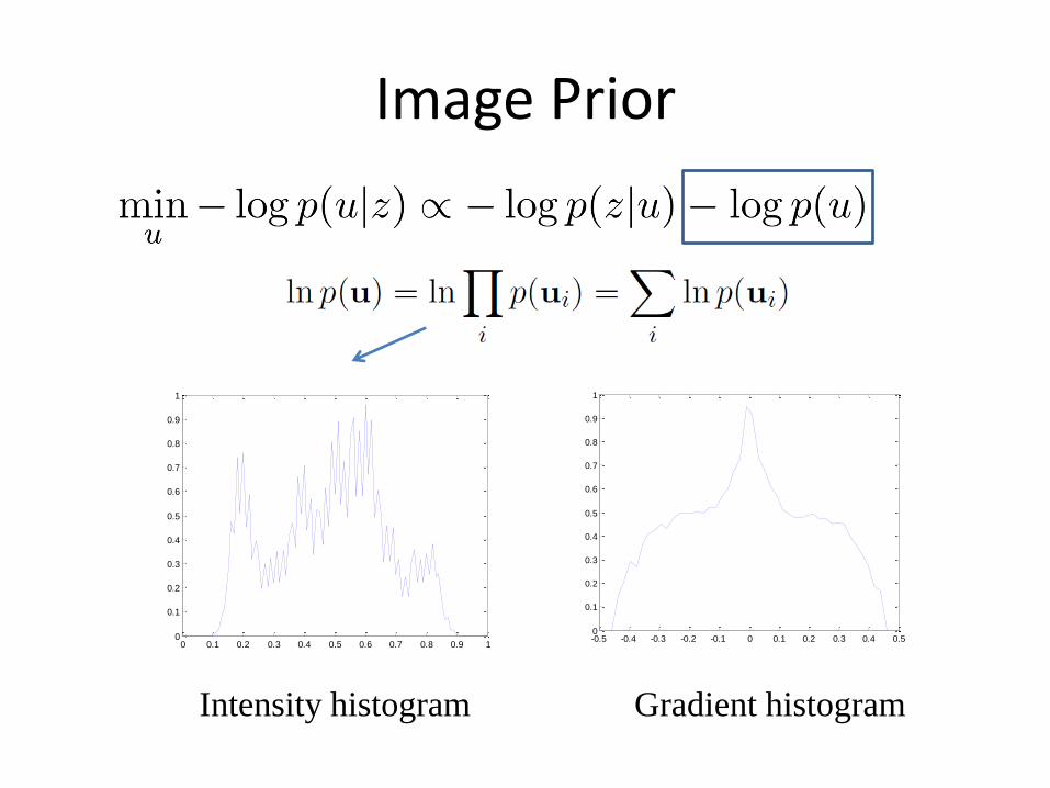
Image Prior
0 0.1 0.2 0.3 0.4 0.5 0.6 0.7 0.8 0.9 10
0.1
0.2
0.3
0.4
0.5
0.6
0.7
0.8
0.9
1
Intensity histogram Gradient histogram
-0.5 -0.4 -0.3 -0.2 -0.1 0 0.1 0.2 0.3 0.4 0.50
0.1
0.2
0.3
0.4
0.5
0.6
0.7
0.8
0.9
1

Image Prior
Gradient histogram
-0.5 -0.4 -0.3 -0.2 -0.1 0 0.1 0.2 0.3 0.4 0.50
0.1
0.2
0.3
0.4
0.5
0.6
0.7
0.8
0.9
1
Theory on when we can do this will be given later (CRF)
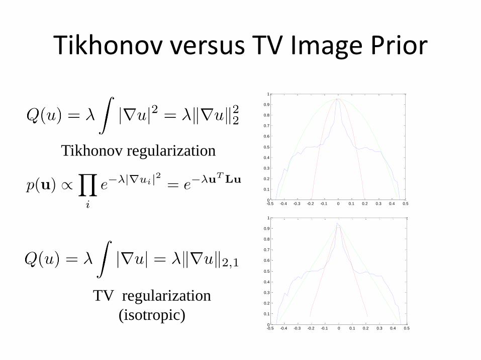
Tikhonov versus TV Image Prior
Tikhonov regularization
TV regularization
(isotropic)
-0.5 -0.4 -0.3 -0.2 -0.1 0 0.1 0.2 0.3 0.4 0.50
0.1
0.2
0.3
0.4
0.5
0.6
0.7
0.8
0.9
1
-0.5 -0.4 -0.3 -0.2 -0.1 0 0.1 0.2 0.3 0.4 0.50
0.1
0.2
0.3
0.4
0.5
0.6
0.7
0.8
0.9
1

Non-convex Image Prior
Non-convex regularization

Bayesian MAP approach for denoising

Analysis-based sparsity
• TV regularization can be extended to other sparse representations
• W often a set of convolutions with highpass filters – Wavelets (property of the Daubechie wavelets) – Learned by PCA

Synthesis-based sparsity
Bayesian approach applied on transform coefficients:
(for a Parseval frame W) PETER G. CASAZZA AND JANET C. TREMAIN: A BRIEF INTRODUCTION TO HILBERT SPACE FRAME THEORY AND ITS APPLICATIONS

Measures of sparsity
• norms
• norm, counts nonzero elements
• many other sparsity measures – smooth l1
• l1 is the only sparsity enforcing convex p-norm

l2 unit ball

l1 unit ball

l0.9 unit ball

l0.5 unit ball

l2-norm

l1-norm

Deblurring
• Denoising
• Deblurring

Super-resolution (with deblurring)
Several possibly shifted blurred images
Di … downsampling operator
Convolutions represent also the shift

Super-resolution
http://zoi.utia.cas.cz/bsr-toolbox

Optical flow
• Based on the assumption of constant brightness and Taylor series
• Optical flow is the velocity field

Regularization
term
Data
term Weighting
parameter
Optical flow

JPEG compression
C TQ
C-1 Q-1
y
x

50 jpg

Bayesian MAP restoration
MAP – maximum a posteriori probability C … 2D cosine transform (orthogonal 64x64 operator) Q … diagonal quantization operator (division by entries qi of the quantization table)

Bayesian JPEG decompression
(Bredies and Holler, 2012)
Or using redundant wavelets
Using total variation (TV)
C … 2D cosine transform (orthogonal 64x64 operator) Q … diagonal quantization operator (division by entries qi of the quantization table)

50 jpg

50 est

45

Convex variational problems
• Denoising, deblurring, SR, optical flow, JPEG decompression …
• Solution by convex optimization (interior point, proximal methods) N. Parikh, S. Boyd: Proximal Algorithms
• What to do for discrete or non-convex problems such as segmentation and stereo?

• For each site (pixel) we look for a label (or a vector of labels)
• Labels depend on local image content and a smoothness constraint
• Image restoration, segmentation, stereo, and optical flow are all labeling problems
Discrete labeling problems
47

• For each site (pixel) we look for a label (or a vector of labels)
• Labels depend on local image content and a smoothness constraint
Discrete labeling problems
48
Segmentation foreground/background or object number
{0,1} {1.. k}
Stereo disparity (inverse depth) -k..k
Optical flow local motion vector (-k..k) x (-k..k)
Restoration intensity 0..255

Segmentation by graph cuts
49

Graph cuts & Belief propagation „Classical local algorithms“
Belief propagation
Graph cuts
50

• Markov Random Field, Gibbs Random Field
– MRF ⇔ GRF (Hammersley-Clifford theorem)
• MRF models including smoothness priors
– stereo
– segmentation
– restoration (denoising, deblurring)
• Discrete optimization on MRFs based on graph cuts
Markov Random Fields (MRFs)
51

• sites S = {1, ... , m} • F ... set of random variables defined on S • N ... neighborhood system • ... (possibly discrete) label • configuration f = {f1 ... fK},
• Other possible properties – homogeneity, isotropy
Markov Random Field (MRF)
52

Gibbs Random Field
Partition function
Energy function U(f)
Vc(f) ... clique potentials
P(f) > 0 !
53

MRF = GRF F is an MRF on S with respect to N if and only if F is a Gibbs random field on S with respect to N MRF ... conditional independence of non-neighbor nodes
(variables) GRF ... global function depending on local “compatability
functions”
Hammersley-Clifford theorem
54
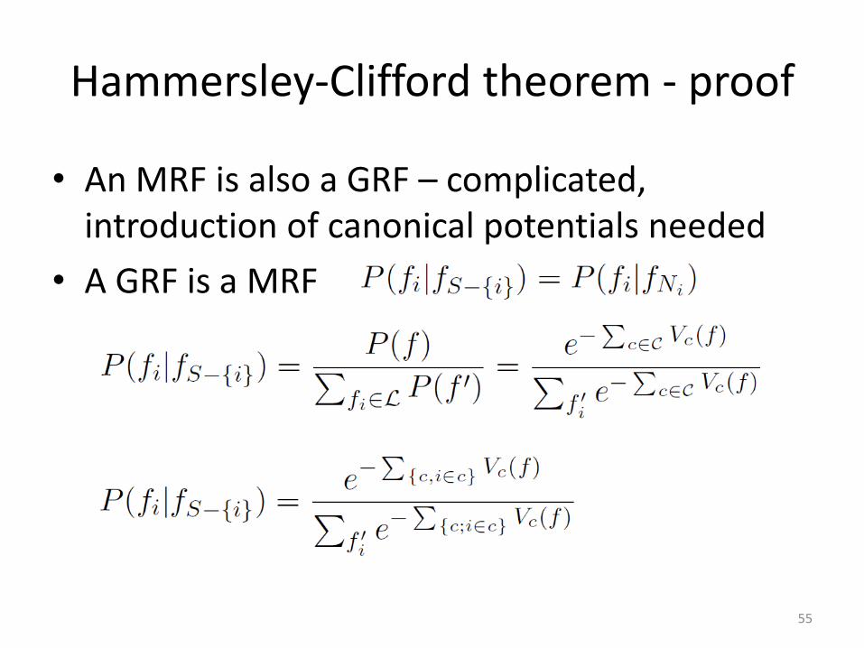
• An MRF is also a GRF – complicated, introduction of canonical potentials needed
• A GRF is a MRF
Hammersley-Clifford theorem - proof
55

• MAP-MRF
• How to incorporate smoothness? – Penalties/potentials similar for most applications
56
MRF = GRF

Priors on derivatives, usually first derivative
Discontinuity preserving penalties
Smoothness prior
57
segmentation, sometimes in stereo
Tikhonov regularization
TV regularization
line process, Mumford-Shah functional

2 images d1,d2 on the input
Birchfield-Tomasi matching cost – insensitive to sampling:
MAP-MRF for stereo (Boykov & al.)
58

“ “GrabCut” — Interactive Foreground Extraction using Iterated Graph Cuts”, C. Rother, V. Kolmogorov, A. Blake, SIGGRAPH 2004
59
MAP-MRF for segmentation

• “Grab cut” example
V1(fi,di) ~ probability to be in fg/bg based on a feature space (intensities, texture features etc...) – modeled for example as a mixture of Gaussians
MAP-MRF for segmentation
60

• Denoising (with anisotropic TV regularization) – 2D indexing - only this slide
• Deblurring (with TV regularization)
• Discrete methods not efficient for restoration!
MAP-MRF for restoration
61

• Common framework for many image processing a CV problems
• Fits well to the Bayesian framework
• MRF = GRF
MRFs - Summary
62
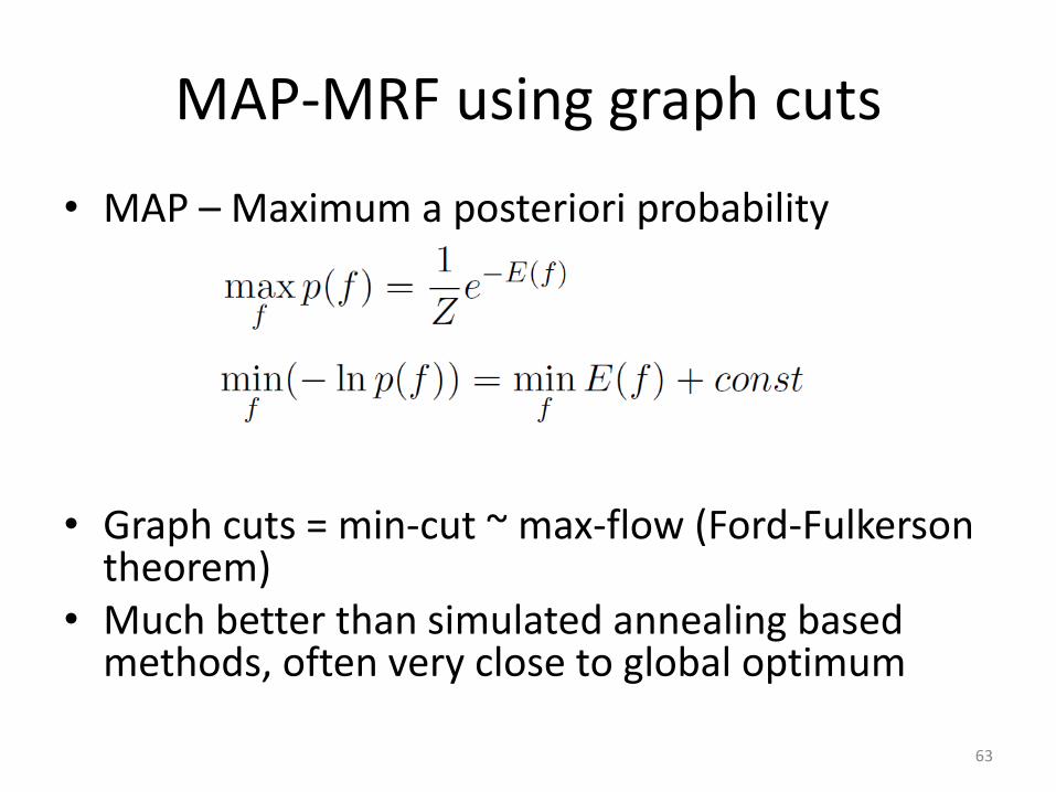
• MAP – Maximum a posteriori probability
• Graph cuts = min-cut ~ max-flow (Ford-Fulkerson theorem)
• Much better than simulated annealing based methods, often very close to global optimum
MAP-MRF using graph cuts
63
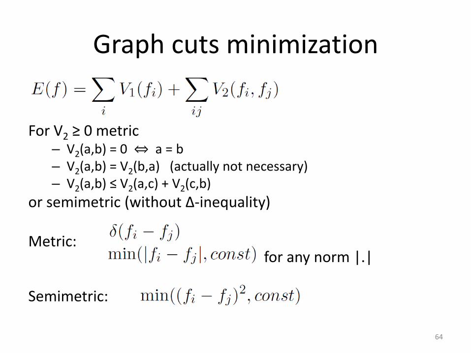
For V2 ≥ 0 metric
– V2(a,b) = 0 ⇔ a = b – V2(a,b) = V2(b,a) (actually not necessary) – V2(a,b) ≤ V2(a,c) + V2(c,b)
or semimetric (without ∆-inequality) Metric:
for any norm |.| Semimetric:
Graph cuts minimization
64

• General strategy – minimum if no possible decrease of E(f) in one “move”
• Iterated conditional modes (ICM) iteratively minimizes each node (pixel) easily gets trapped in a local minimum (~ gradient descent)
• Simulated annealing – global moves but without any specific direction slow
• Graph cuts – use much larger set of “moves” so that the minimum over the whole set can be found in a reasonable (polynomial) time
Graph cuts minimization
65

α-β swap and α-expansion moves
initial labeling single pixel ICM move
α-β swap move α-expansion
move
66
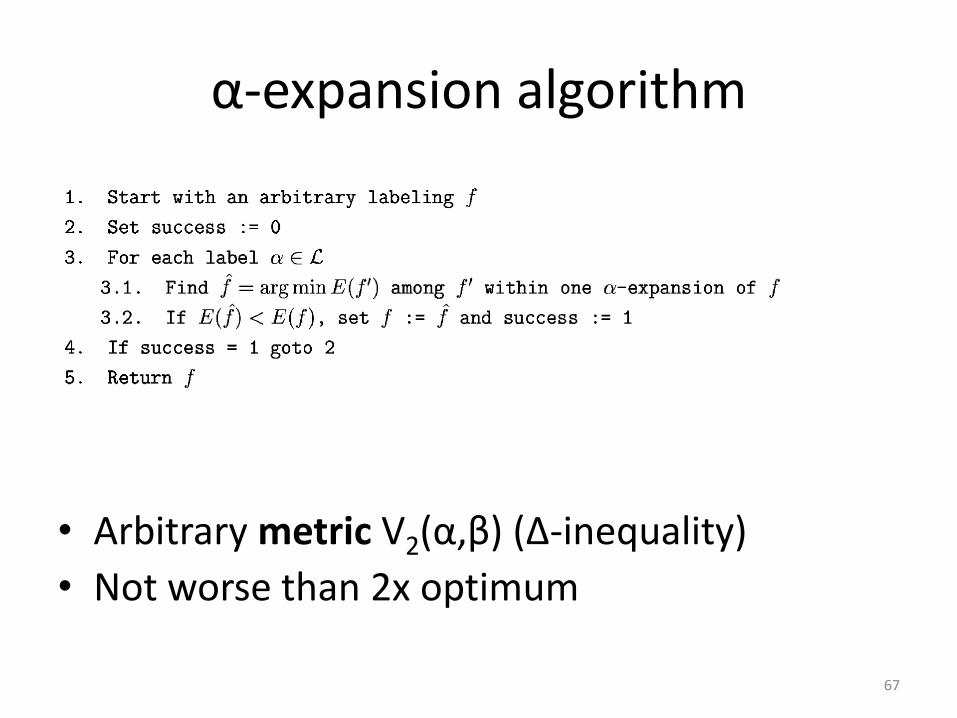
• Arbitrary metric V2(α,β) (Δ-inequality)
• Not worse than 2x optimum
α-expansion algorithm
67

• Arbitrary semimetric V2(α,β) (without Δ-inequality)
• No optimality guaranteed
α-β swap algorithm
68

α-β swap move graph
69

α-β swap move graph
70

α-β swap move graph
71
Proof step 1: For each p in the set Pαβ, the minimum cut contains exactly one edge tp

α-β swap move graph
72
Proof step 2: go through 3 types of pairwise configurations. We need binary V to be semi-metric V(α,α)=0

• We know how to transform minimization of E(f) over all possible α-β swap moves to graph cut problem
73
α-β swap - summary

α-expansion move graph
74

α-expansion move graph
75

∆ - inequality !
α-expansion graph - cuts
76

• We know how to transform minimization of E(f) over all possible α-expansion moves to graph cut problem
• What remains? - how to find the minimum cut
77
α-expansion - summary

• “Augmenting path” type algorithm with simple heuristics – Looks for a non-saturated path ~ path in residual
graph – Simultaneously builds trees from α and β
• Maximum complexity O(n2mCmax), Cmax cost of the minimum cut
• Actually typically linear with respect to the number of pixels
• On our problems faster than good combinatorial algorithms - Dinic O(n2m), Push-relabel O(n2√m)
Graph cuts algorithm
78

• Minimization of E(f) by finding min-cut in a graph in polynomial time
2 label minimization can be done in polynomial (and typically linear) time with respect to the number of pixels
• K>2 labels – NP hard – Equivalent to Multiway Cut Problem – α-expansion finds a solution ≤ 2*optimum – In practice both α-β swap and α-expansion algorithms get very
close to global minimum
Graph cuts - summary
79

“ “GrabCut” — Interactive Foreground Extraction using Iterated Graph Cuts”, C. Rother, V. Kolmogorov, A. Blake, SIGGRAPH 2004
80
Graph cuts – additional example

• Conditional independence is strong structural information that can be exploited
• Gives useful approximations for difficult (NP-hard) problems
• For convex problems mostly better to use continuous methods
Discrete optimization in MRFs - summary
81

• Graph Cuts – “Fast Approximate Energy Minimization via Graph Cuts” - Y.
Boykov, O. Veksler, R. Zabih, PAMI 2001 (Augmenting path min-cut algorithm)
– “An Experimental Comparison of Min-Cut/Max-flow Algorithms for Energy Minimization in Vision” – Y. Boykov, V. Kolmogorov, PAMI 2004 (Graph construction for α-β swap and α-expansion moves)
– “ “GrabCut” — Interactive Foreground Extraction using Iterated Graph Cuts”, C. Rother, V. Kolmogorov, A. Blake, SIGGRAPH 2004
• Belief propagation – “Understanding Belief Propagation and its Generalizations” -
J.S. Yedidia, W.T.Freeman, Y.Weiss (Mitsubishi electric research laboratories, Technical report, 2002)
References
82

• Continuous counterpart of Ishikawa’s pairwise MRF problem taking huge memory
• “Arbitrary” non-convex data term
Convex formulation of multi-label problems
Pock, Schoenemann, Graber, Bischof, Cremers: A Convex Formulation of Continuous Multi-label Problems (2008)

Functional lifting
Layer cake formula
Representing u in terms of its level sets

Mathematics in image processing
Many image processing/CV problems can be formulated as optimization problems and solved by variational or discrete algorithms within a common framework
– image restoration (denoising, deblurring, SR, JPEG decompression)
– image segmentation
– optical flow
– stereo