MATLAB Chapter 4

1

MATLAB Course November-December 2006

Chapter 4: Optimization

>> help fminunc FMINUNC Finds the minimum of a function of several variables. X=FMINUNC(FUN,X0) starts at X0 and finds a minimum X of the function FUN. FUN accepts input X and returns a scalar function value F evaluated at X. X0 can be a scalar, vector or matrix. X=FMINUNC(FUN,X0,OPTIONS) minimizes with the default optimization parameters replaced by values in the structure OPTIONS, an argument created with the OPTIMSET function. See OPTIMSET for details. Used options are Display, TolX, TolFun, DerivativeCheck, Diagnostics, GradObj, HessPattern, LineSearchType, Hessian, HessMult, HessUpdate, MaxFunEvals, MaxIter, DiffMinChange and DiffMaxChange, LargeScale, MaxPCGIter, PrecondBandWidth, TolPCG, TypicalX. Use the GradObj option to specify that FUN also returns a second output argument G that is the partial derivatives of the function df/dX, at the point X. Use the Hessian option to specify that FUN also returns a third output argument H that is the 2nd partial derivatives of the function (the Hessian) at the point X. The Hessian is only used by the large-scale method, not the line-search method. X=FMINUNC(FUN,X0,OPTIONS,P1,P2,...) passes the problem-dependent parameters P1,P2,... directly to the function FUN, e.g. FUN would be called using feval as in: feval(FUN,X,P1,P2,...). Pass an empty matrix for OPTIONS to use the default values. [X,FVAL]=FMINUNC(FUN,X0,...) returns the value of the objective function FUN at the solution X. [X,FVAL,EXITFLAG]=FMINUNC(FUN,X0,...) returns a string EXITFLAG that describes the exit condition of FMINUNC. If EXITFLAG is: > 0 then FMINUNC converged to a solution X. 0 then the maximum number of function evaluations was reached. < 0 then FMINUNC did not converge to a solution.

[X,FVAL,EXITFLAG,OUTPUT]=FMINUNC(FUN,X0,...) returns a structure OUTPUT with the number of iterations taken in OUTPUT.iterations, the number of function evaluations in OUTPUT.funcCount, the algorithm used in

MATLAB Chapter 4

2

OUTPUT.algorithm, the number of CG iterations (if used) in OUTPUT.cgiterations, and the first-order optimality (if used) in OUTPUT.firstorderopt.

[X,FVAL,EXITFLAG,OUTPUT,GRAD]=FMINUNC(FUN,X0,...) returns the value of the gradient of FUN at the solution X. [X,FVAL,EXITFLAG,OUTPUT,GRAD,HESSIAN]=FMINUNC(FUN,X0,...) returns the value of the Hessian of the objective function FUN at the solution X. Examples FUN can be specified using @: X = fminunc(@myfun,2) where MYFUN is a MATLAB function such as: function F = myfun(x) F = sin(x) + 3; To minimize this function with the gradient provided, modify the MYFUN so the gradient is the second output argument: function [f,g]= myfun(x) f = sin(x) + 3; g = cos(x); and indicate the gradient value is available by creating an options structure with OPTIONS.GradObj set to 'on' (using OPTIMSET): options = optimset('GradObj','on'); x = fminunc('myfun',4,options); FUN can also be an inline object: x = fminunc(inline('sin(x)+3'),4); See also OPTIMSET, FMINSEARCH, FMINBND, FMINCON, @, INLINE.

MATLAB Chapter 4

3

Example 1

Minimize the function 4 3 212.

4y x x x= − + +

Note the derivative of y w.r.t. x is g=3 23 2 ,x x x− + which is equal to zero for -1, 0 and 2. function xn=example1(x0) x=-2:.1:3; y=(1/4)*x.^4-x.^3+x.^2+2; g=x.^3-3*x.^2+2*x; [x;y;g] plot(x,y) axis([-2 3 0 5]) options=optimset('Diagnostics','on','Display','iter','GradObj','off','Hessian','off',… 'LargeScale','off','DerivativeCheck','on','TolFun',1E-8); [xn,fval,exitflag,output,grad] = fminunc('func1',x0,options) if exitflag ~= 1 xn,fval,exitflag,output,grad,error('convergence error') end function f=func1(x) f=(1/4)*x^4-x^3+x^2+2;

MATLAB Chapter 4

4

>> xn=example1(-3) ans = Columns 1 through 8 -1.0000 -0.9000 -0.8000 -0.7000 -0.6000 -0.5000 -0.4000 -0.3000 4.2500 3.7030 3.2544 2.8930 2.6084 2.3906 2.2304 2.1190 -6.0000 -4.9590 -4.0320 -3.2130 -2.4960 -1.8750 -1.3440 -0.8970 Columns 9 through 16 -0.2000 -0.1000 0 0.1000 0.2000 0.3000 0.4000 0.5000 2.0484 2.0110 2.0000 2.0090 2.0324 2.0650 2.1024 2.1406 -0.5280 -0.2310 0 0.1710 0.2880 0.3570 0.3840 0.3750 Columns 17 through 24 0.6000 0.7000 0.8000 0.9000 1.0000 1.1000 1.2000 1.3000 2.1764 2.2070 2.2304 2.2450 2.2500 2.2450 2.2304 2.2070 0.3360 0.2730 0.1920 0.0990 0 -0.0990 -0.1920 -0.2730 Columns 25 through 32 1.4000 1.5000 1.6000 1.7000 1.8000 1.9000 2.0000 2.1000 2.1764 2.1406 2.1024 2.0650 2.0324 2.0090 2.0000 2.0110 -0.3360 -0.3750 -0.3840 -0.3570 -0.2880 -0.1710 0 0.2310 Columns 33 through 41 2.2000 2.3000 2.4000 2.5000 2.6000 2.7000 2.8000 2.9000 3.0000 2.0484 2.1190 2.2304 2.3906 2.6084 2.8930 3.2544 3.7030 4.2500 0.5280 0.8970 1.3440 1.8750 2.4960 3.2130 4.0320 4.9590 6.0000 %%%%%%%%%%%%%%%%%%%%%%%%%%%%%%%%%%%%%%%%%%% Diagnostic Information Number of variables: 1 Functions Objective: (1/4)*x^4-x^3+x^2+2 Gradient: finite-differencing Hessian: finite-differencing (or Quasi-Newton) Algorithm selected medium-scale: Quasi-Newton line search %%%%%%%%%%%%%%%%%%%%%%%%%%%%%%%%%%%%%%%%%%% End diagnostic information

MATLAB Chapter 4

5

First-order Iteration Func-count f(x) Step-size optimality 0 2 58.25 60 1 4 18 0.0166667 24 2 6 6.93827 1 10.4 3 8 3.36258 1 4.26 4 10 2.34035 1 1.72 5 12 2.06774 1 0.642 6 14 2.00896 1 0.206 7 16 2.00054 1 0.0475 8 18 2.00001 1 0.00553 9 20 2 1 0.000184 10 22 2 1 7.15e-007 11 24 2 1 2.98e-008 Optimization terminated: relative infinity-norm of gradient less than options.TolFun. xn =

-2.4513e-009 fval =

2 exitflag =

1 output = iterations: 11 funcCount: 24 stepsize: 1 firstorderopt: 2.9802e-008 algorithm: 'medium-scale: Quasi-Newton line search' grad =

-2.9802e-008 ans=

-2.4513e-009

MATLAB Chapter 4

6

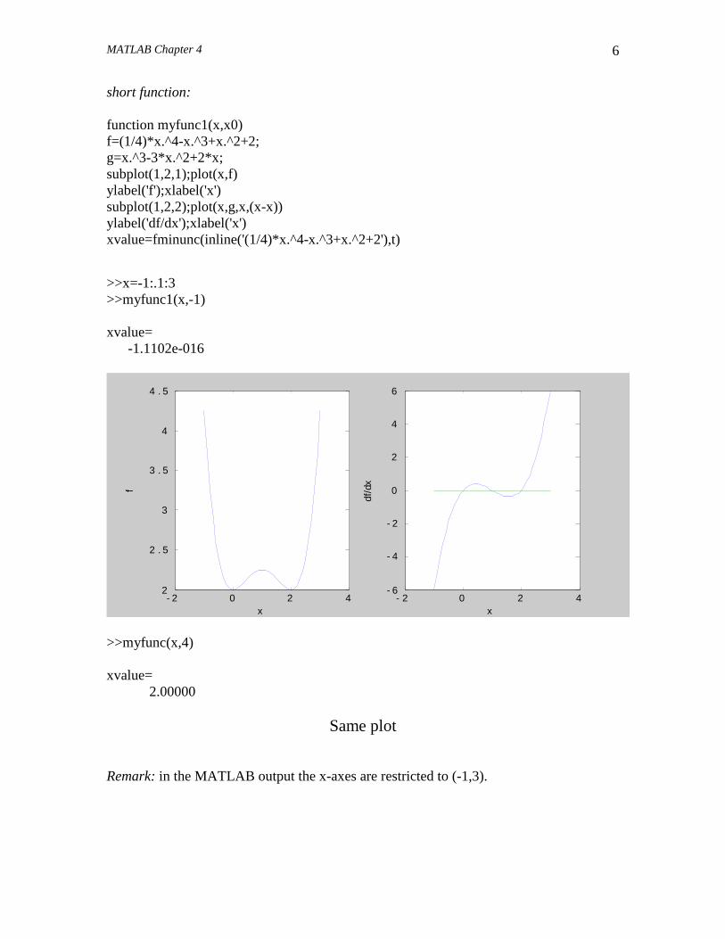
short function: function myfunc1(x,x0) f=(1/4)*x.^4-x.^3+x.^2+2; g=x.^3-3*x.^2+2*x; subplot(1,2,1);plot(x,f) ylabel('f');xlabel('x') subplot(1,2,2);plot(x,g,x,(x-x)) ylabel('df/dx');xlabel('x') xvalue=fminunc(inline('(1/4)*x.^4-x.^3+x.^2+2'),t) >>x=-1:.1:3 >>myfunc1(x,-1) xvalue= -1.1102e-016

- 2 0 2 42

2 . 5

3

3 . 5

4

4 . 5

f

x- 2 0 2 4

- 6

- 4

- 2

0

2

4

6

df/d

x

x >>myfunc(x,4) xvalue=

2.00000

Same plot

Remark: in the MATLAB output the x-axes are restricted to (-1,3).

MATLAB Chapter 4

7

Example 2 Minimize the function 2 2 2

1 2 1( ) ( ) (1 ) .f x x x= − + −x

function xn=example2(x) options=optimset('Diagnostics','on','Display','iter','GradObj','off',... 'Hessian','off','LargeScale','off','DerivativeCheck','on','TolFun',1E-8); [xn,fval,exitflag,output,grad] = fminunc('func2',x,options) if exitflag ~= 1 xn,fval,exitflag,output,grad,error('convergence error') end function [f,g]=func2(x) f=(x(1)^2-x(2))^2+(1-x(1))^2; >> xn=example2([.5 .5]) %%%%%%%%%%%%%%%%%%%%%%%%%%%%%%%%%%%%%%%%%%% Diagnostic Information Number of variables: 2 Functions Objective: func2 Gradient: finite-differencing Hessian: finite-differencing (or Quasi-Newton) Algorithm selected medium-scale: Quasi-Newton line search %%%%%%%%%%%%%%%%%%%%%%%%%%%%%%%%%%%%%%%%%% End diagnostic information First-order Iteration Func-count f(x) Step-size optimality 0 3 0.3125 1.5 1 9 0.0854609 0.177087 0.349 2 12 0.0716593 1 0.238 3 15 0.0331821 1 0.301 4 18 0.00472458 1 0.175 5 21 4.37497e-005 1 0.0246 6 24 2.80563e-006 1 0.00424 7 27 6.40314e-011 1 1.32e-005 8 30 9.51925e-015 1 1.38e-007 9 33 2.7754e-015 1 1.03e-010 Optimization terminated: relative infinity-norm of gradient less than options.TolFun.

MATLAB Chapter 4

8

xn = 1.0000 1.0000 fval = 2.7754e-015 exitflag = 1 output = iterations: 9 funcCount: 33 stepsize: 1 firstorderopt: 1.0337e-010 algorithm: 'medium-scale: Quasi-Newton line search' message: [1x85 char] grad = 1.0e-009 * -0.1034 0.0496 xn = 1.0000 1.0000

MATLAB Chapter 4

9

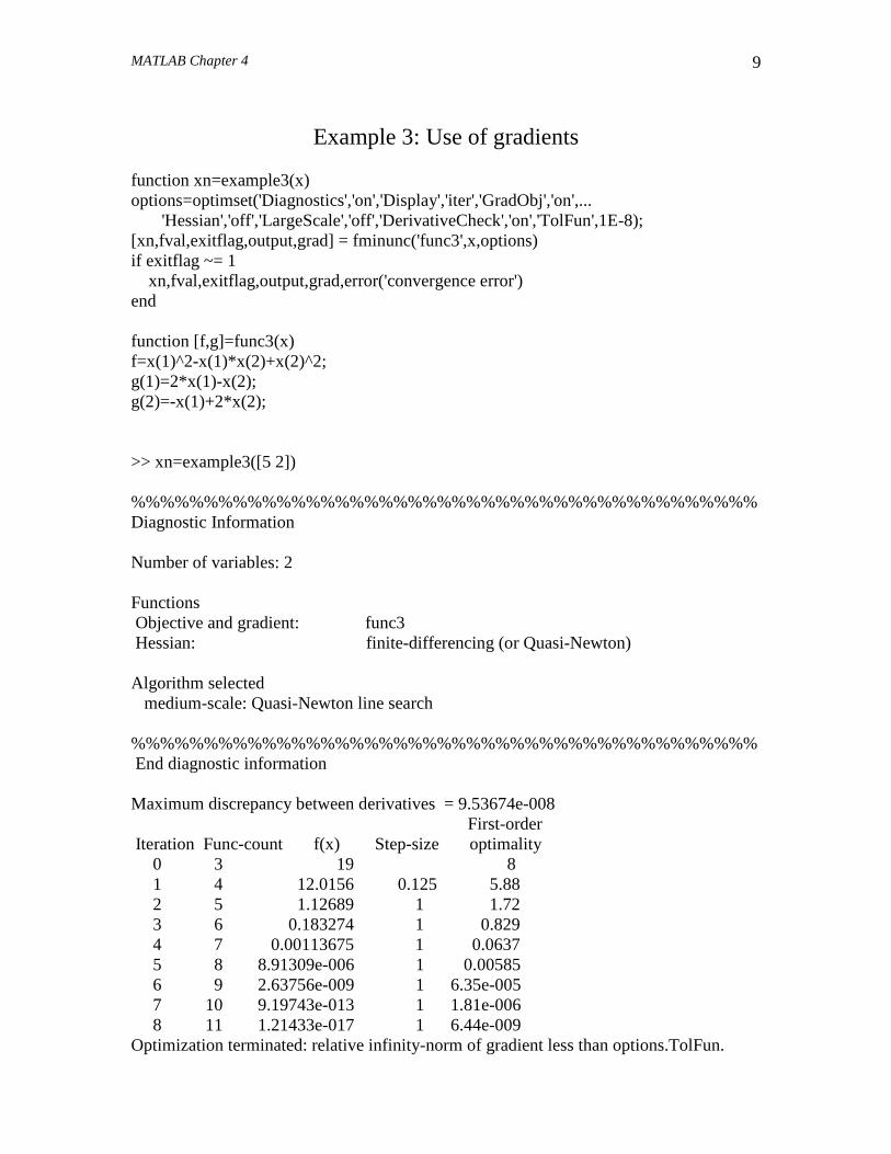
Example 3: Use of gradients function xn=example3(x) options=optimset('Diagnostics','on','Display','iter','GradObj','on',... 'Hessian','off','LargeScale','off','DerivativeCheck','on','TolFun',1E-8); [xn,fval,exitflag,output,grad] = fminunc('func3',x,options) if exitflag ~= 1 xn,fval,exitflag,output,grad,error('convergence error') end function [f,g]=func3(x) f=x(1)^2-x(1)*x(2)+x(2)^2; g(1)=2*x(1)-x(2); g(2)=-x(1)+2*x(2); >> xn=example3([5 2]) %%%%%%%%%%%%%%%%%%%%%%%%%%%%%%%%%%%%%%%%%%% Diagnostic Information Number of variables: 2 Functions Objective and gradient: func3 Hessian: finite-differencing (or Quasi-Newton) Algorithm selected medium-scale: Quasi-Newton line search %%%%%%%%%%%%%%%%%%%%%%%%%%%%%%%%%%%%%%%%%%% End diagnostic information Maximum discrepancy between derivatives = 9.53674e-008 First-order Iteration Func-count f(x) Step-size optimality 0 3 19 8 1 4 12.0156 0.125 5.88 2 5 1.12689 1 1.72 3 6 0.183274 1 0.829 4 7 0.00113675 1 0.0637 5 8 8.91309e-006 1 0.00585 6 9 2.63756e-009 1 6.35e-005 7 10 9.19743e-013 1 1.81e-006 8 11 1.21433e-017 1 6.44e-009 Optimization terminated: relative infinity-norm of gradient less than options.TolFun.

MATLAB Chapter 4

10

xn = 1.0e-008 * 0.2455 -0.1534 fval = 1.2143e-017 exitflag = 1 output = iterations: 8 funcCount: 11 stepsize: 1 firstorderopt: 6.4432e-009 algorithm: 'medium-scale: Quasi-Newton line search' message: [1x85 char] grad = 1.0e-008 * 0.6443 -0.5522 xn = 1.0e-008 * 0.2455 -0.1534

MATLAB Chapter 4

11

Examples 4 and 5: Factor Analysis Assume we have 4 variables and want to fit a one factor model. In the example here the sample size is 649. So the model equations are

' ,= +Σ λλ Ψ where Ψ is a diagonal matrix. Furthermore, the least squares function can be written as

2 2

1 1

( ) ( )p p

ij iji j

f s trσ= =

= − = −∑∑ S Σ

The vector “x” in MATLAB contains here first the 4 factor loadings and then the 4 error variances. function example4 S=[86.3979 57.7751 56.8651 58.8986;…. 57.7751 86.2632 59.3177 59.6683;… 56.8651 59.3177 97.2850 73.8201;… 58.8986 59.6683 73.8201 97.8192] x=rand(1,8) options=optimset('Diagnostics','on','Display','iter','GradObj','off',... 'Hessian','off','LargeScale','off','DerivativeCheck','on','TolFun',1E-8); [xn,fval,exitflag,output,grad] = fminunc('func4',x,options,S) if exitflag ~= 1 xn,fval,exitflag,output,grad,error('convergence error') end 'solution' LAB=xn(1:4)' PSI=diag(xn(5:8)) fval function f=func4(x,S) LAB=x(1:4)'; PSI=diag(x(5:8)); SIG=LAB*LAB'+PSI; f=trace((S-SIG)^2);

MATLAB Chapter 4

12

>> example4 S = 86.3979 57.7751 56.8651 58.8986 57.7751 86.2632 59.3177 59.6683 56.8651 59.3177 97.2850 73.8201 58.8986 59.6683 73.8201 97.8192 x = 0.8214 0.4447 0.6154 0.7919 0.9218 0.7382 0.1763 0.4057 %%%%%%%%%%%%%%%%%%%%%%%%%%%%%%%%%%%%%%%%%%% Diagnostic Information Number of variables: 8 Functions Objective: func4 Gradient: finite-differencing Hessian: finite-differencing (or Quasi-Newton) Algorithm selected medium-scale: Quasi-Newton line search %%%%%%%%%%%%%%%%%%%%%%%%%%%%%%%%%%%%%%%%%%% End diagnostic information First-order Iteration Func-count f(x) Step-size optimality 0 9 77691.1 784 1 36 2900.05 0.0100889 781 2 63 2597.36 0.0134495 350 3 81 2500.67 0.123056 49.2 4 99 1729.6 10 266 5 117 973.247 0.1484 758 6 126 252.255 1 472 7 144 158.88 0.1 125 8 153 116.702 1 26 9 162 116.259 1 3.5 10 171 116.242 1 0.636 11 180 116.229 1 1.78 12 189 116.173 1 6.07 13 198 116.092 1 9 14 207 115.989 1 8.47 15 216 115.937 1 3.98 16 225 115.927 1 0.677 17 234 115.926 1 0.0216

MATLAB Chapter 4

13

First-order Iteration Func-count f(x) Step-size optimality 18 243 115.926 1 0.0206 19 252 115.926 1 0.0272 20 261 115.926 1 0.0416 21 270 115.926 1 0.0508 22 279 115.926 1 0.0434 23 288 115.926 1 0.0195 24 297 115.926 1 0.00316 25 306 115.926 1 0.00285 26 315 115.926 1 0.00271 27 324 115.926 1 0.00255 28 333 115.926 1 0.00251 29 342 115.926 1 0.00195 30 351 115.926 1 0.000894 31 360 115.926 1 0.000338 32 369 115.926 1 5.84e-005 33 378 115.926 1 5.16e-006 Optimization terminated: relative infinity-norm of gradient less than options.TolFun. xn = 7.1752 7.3601 8.2932 8.4502 34.9144 32.0915 28.5079 26.4140 fval = 115.9256 exitflag = 1 output = iterations: 33 funcCount: 378 stepsize: 1 firstorderopt: 5.1630e-006 algorithm: 'medium-scale: Quasi-Newton line search' grad = 1.0e-005 * -0.0665 -0.0648 -0.2415 0.0113 0.4698 -0.1189 0.0167 -0.5163

MATLAB Chapter 4

14

ans = solution LAB = 7.1752 7.3601 8.2932 8.4502 PSI = 34.9144 0 0 0 0 32.0915 0 0 0 0 28.5079 0 0 0 0 26.4140 fval = 115.9256

MATLAB Chapter 4

15

We now perform a 2 factor model of the form

'= +Σ ΛΦΛ Ψ , where the matrices have the following form

0

0

0

0

1

1

0 0 0

0 0 0

0 0 0

0 0 0

αα

ββρ

ργ

γδ

δ

=

=

=

Λ

Φ

Ψ

In the MATLAB program we define the vector x as: ( ).x α β γ δ ρ= So there are 5 unknown parameters. In the program we start with random start values. function example5 S=[86.3979 57.7751 56.8651 58.8986;... 57.7751 86.2632 59.3177 59.6683;... 56.8651 59.3177 97.2850 73.8201;... 58.8986 59.6683 73.8201 97.8192] x=rand(1,5) options=optimset('Diagnostics','on','Display','iter','GradObj','off',... 'Hessian','off','LargeScale','off','DerivativeCheck','on','TolFun',1E-8); [xn,fval,exitflag,output,grad] = fminunc('func5',x,options,S) if exitflag ~= 1 xn,fval,exitflag,output,grad,error('convergence error') end 'solution' LAB=[xn(1) 0;xn(1) 0;0 xn(2);0 xn(2)] PHI=[1 xn(5);xn(5) 1] PSI=diag([xn(3) xn(3) xn(4) xn(4)]) SIG=LAB*PHI*LAB'+PSI S-SIG f=func5(xn,S)

MATLAB Chapter 4

16

function f=func5(x,S) LAB=[x(1) 0;x(1) 0;0 x(2);0 x(2)]; PHI=[1 x(5);x(5) 1]; PSI=diag([x(3) x(3) x(4) x(4)]); SIG=LAB*PHI*LAB'+PSI; f=trace((S-SIG)^2); >> example5 S = 86.3979 57.7751 56.8651 58.8986 57.7751 86.2632 59.3177 59.6683 56.8651 59.3177 97.2850 73.8201 58.8986 59.6683 73.8201 97.8192 x = 0.8216 0.6449 0.8180 0.6602 0.3420 %%%%%%%%%%%%%%%%%%%%%%%%%%%%%%%%%%%%%%%%%%% Diagnostic Information Number of variables: 5 Functions Objective: func5 Gradient: finite-differencing Hessian: finite-differencing (or Quasi-Newton) Algorithm selected medium-scale: Quasi-Newton line search %%%%%%%%%%%%%%%%%%%%%%%%%%%%%%%%%%%%%%%%%%% End diagnostic information First-order Iteration Func-count f(x) Step-size optimality 0 6 77700.6 1.14e+003 1 36 21337.2 0.00416643 6.56e+003 2 54 21082.8 0.0431329 9.69e+003 3 66 5824.02 0.5 3.87e+003 4 84 4887.96 0.091649 1.13e+004 5 90 2429.54 1 7.31e+003 6 96 1178.28 1 3.02e+003 7 102 1069.89 1 1.24e+003 8 108 1055.38 1 143 9 114 1050.72 1 97.2 10 120 1048.97 1 49

MATLAB Chapter 4

17

First-order Iteration Func-count f(x) Step-size optimality 11 126 1041.28 1 164 12 132 1024.36 1 420 13 138 978.007 1 842 … … ……… . … 31 246 9.60156 1 1.74 32 252 9.60141 1 0.0904 33 258 9.60141 1 0.0188 34 264 9.60141 1 0.000627 35 270 9.60141 1 2.38e-006 Optimization terminated: relative infinity-norm of gradient less than options.TolFun. xn = 7.6010 8.5919 28.5555 23.7320 0.8986 fval = 9.6014 exitflag = 1 output = iterations: 35 funcCount: 270 stepsize: 1 firstorderopt: 2.3842e-006 algorithm: 'medium-scale: Quasi-Newton line search' grad = 1.0e-005 * -0.0235 -0.1804 -0.0083 -0.0045 -0.2384 ans = solution LAB = 7.6010 0 7.6010 0 0 8.5919 0 8.5919

MATLAB Chapter 4

18

PHI = 1.0000 0.8986 0.8986 1.0000 PSI = 28.5555 0 0 0 0 28.5555 0 0 0 0 23.7320 0 0 0 0 23.7320 SIG = 86.3305 57.7751 58.6874 58.6874 57.7751 86.3305 58.6874 58.6874 58.6874 58.6874 97.5521 73.8201 58.6874 58.6874 73.8201 97.5521 ans = 0.0674 0.0000 -1.8223 0.2112 0.0000 -0.0673 0.6303 0.9809 -1.8223 0.6303 -0.2671 0.0000 0.2112 0.9809 0.0000 0.2671 f = 9.6014

MATLAB Chapter 4

19

Example 6: Maximum likelihood estimates

The function to be minimized which yields maximum likelihood estimates is

( )1 1( ) log ,f tr p− −= + −Σ S Σ S

where p is the number of variables; here p = 4. A problem with this function may be that during the iterative process the determinant may become negative, i.e. when some of the eigenvalues become negative. Therefore a good start vector is needed. In this example we first compute the least squares estimates of the parameters, and then use this output as starting vector for the maximum likelihood method. P.S. Under the assumption of normality of the variables it holds that the final function value*(n-1) is chi-square distributed with degrees of freedom equal to the total number of (co)variances in the observed covariance matrix (i.e. p(p+1)/2) minus the number of unknown parameters. So in this case df=10 – 5 = 5. function example6 S=[86.3979 57.7751 56.8651 58.8986;... 57.7751 86.2632 59.3177 59.6683;... 56.8651 59.3177 97.2850 73.8201;... 58.8986 59.6683 73.8201 97.8192] ind=0 x=rand(1,5) options=optimset('Diagnostics','off','Display','off','GradObj','off',... 'Hessian','off','LargeScale','off','DerivativeCheck','on','TolFun',1E-6); [xn,fval,exitflag,output,grad] = fminunc('func6',x,options,S,ind) if exitflag ~= 1 xn,fval,exitflag,output,grad, error('convergence error') end ind=1 [xn,fval,exitflag,output,grad] = fminunc('func6',xn,options,S,ind) if exitflag ~= 1 xn,fval,exitflag,output,grad, error('convergence error') end 'solution' LAB=[xn(1) 0;xn(1) 0;0 xn(2);0 xn(2)] PHI=[1 xn(5);xn(5) 1] PSI=diag([xn(3) xn(3) xn(4) xn(4)]) SIG=LAB*PHI*LAB'+PSI S-SIG X2=648*func6(xn,S,ind); % 648=n-1 df=10-length(x); pvalue=1-chi2cdf(X2,df); ‘Chi-square, df, p-value’ [X2 df pvalue]

MATLAB Chapter 4

20

function f=func6(x,S,ind) LAB=[x(1) 0;x(1) 0;0 x(2);0 x(2)]; PHI=[1 x(5);x(5) 1]; PSI=diag([x(3) x(3) x(4) x(4)]); SIG=LAB*PHI*LAB'+PSI; if ind == 0 f=trace((S-SIG)^2); else A=inv(SIG)*S; f=trace(A)-log(det(A))-4; end >> example6 S = 86.3979 57.7751 56.8651 58.8986 57.7751 86.2632 59.3177 59.6683 56.8651 59.3177 97.2850 73.8201 58.8986 59.6683 73.8201 97.8192 ind = 0 x = 0.1536 0.6756 0.6992 0.7275 0.4784 xn = 7.6010 8.5919 28.5555 23.7320 0.8986 fval = 9.6014 exitflag = 1 output = iterations: 32 funcCount: 246 stepsize: 1 firstorderopt: 9.4175e-006 algorithm: 'medium-scale: Quasi-Newton line search'

MATLAB Chapter 4

21

grad = 1.0e-005 * -0.1364 0.0583 -0.0058 0.0146 0.9418 ind = 1 xn = 7.6010 8.5919 28.5555 23.7320 0.8986 fval = 0.0030 exitflag = 1 output = iterations: 0 funcCount: 6 stepsize: [] firstorderopt: 1.7881e-007 algorithm: 'medium-scale: Quasi-Newton line search' message: [1x117 char] grad = 1.0e-006 * 0 0 0.0021 0.0025 0.1788 ans = solution LAB = 7.6010 0 7.6010 0 0 8.5919 0 8.5919

MATLAB Chapter 4

22

PHI = 1.0000 0.8986 0.8986 1.0000 PSI = 28.5555 0 0 0 0 28.5555 0 0 0 0 23.7320 0 0 0 0 23.7320 SIG = 86.3305 57.7751 58.6874 58.6874 57.7751 86.3305 58.6874 58.6874 58.6874 58.6874 97.5521 73.8201 58.6874 58.6874 73.8201 97.5521 ans = 0.0674 0.0000 -1.8223 0.2112 0.0000 -0.0673 0.6303 0.9809 -1.8223 0.6303 -0.2671 0.0000 0.2112 0.9809 0.0000 0.2671 ans = Chi-square, df, p-value ans = 1.9335 5.0000 0.8583 Thus: the chi square value is 1.9335, the degrees of freedom is 5 and the p-level is .8583 .

MATLAB Chapter 4

23

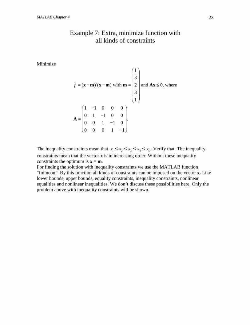
Example 7: Extra, minimize function with all kinds of constraints

Minimize

1

3

( ) '( ) with and , where2

3

1

1 1 0 0 0

0 1 1 0 0.

0 0 1 1 0

0 0 0 1 1

f

= − − = ≤

− − = − −

x m x m m Ax 0

A

The inequality constraints mean that 1 2 3 4 5.x x x x x≤ ≤ ≤ ≤ Verify that. The inequality

constraints mean that the vector x is in increasing order. Without these inequality constraints the optimum is x = m. For finding the solution with inequality constraints we use the MATLAB function “fmincon”. By this function all kinds of constraints can be imposed on the vector x. Like lower bounds, upper bounds, equality constraints, inequality constraints, nonlinear equalities and nonlinear inequalities. We don’t discuss these possibilities here. Only the problem above with inequality constraints will be shown.

MATLAB Chapter 4

24

>> help fmincon FMINCON finds a constrained minimum of a function of several variables. FMINCON attempts to solve problems of the form: min F(X) subject to: A*X <= B, Aeq*X = Beq (linear constraints) X ` C(X) <= 0, Ceq(X) = 0 (nonlinear constraints) LB <= X <= UB X=FMINCON(FUN,X0,A,B) starts at X0 and finds a minimum X to the function FUN, subject to the linear inequalities A*X <= B. FUN accepts input X and returns a scalar function value F evaluated at X. X0 may be a scalar, vector, or matrix. X=FMINCON(FUN,X0,A,B,Aeq,Beq) minimizes FUN subject to the linear equalities Aeq*X = Beq as well as A*X <= B. (Set A=[] and B=[] if no inequalities exist.) X=FMINCON(FUN,X0,A,B,Aeq,Beq,LB,UB) defines a set of lower and upper bounds on the design variables, X, so that a solution is found in the range LB <= X <= UB. Use empty matrices for LB and UB if no bounds exist. Set LB(i) = -Inf if X(i) is unbounded below; set UB(i) = Inf if X(i) is unbounded above. X=FMINCON(FUN,X0,A,B,Aeq,Beq,LB,UB,NONLCON) subjects the minimization to the constraints defined in NONLCON. The function NONLCON accepts X and returns the vectors C and Ceq, representing the nonlinear inequalities and equalities respectively. FMINCON minimizes FUN such that C(X)<=0 and Ceq(X)=0. (Set LB=[] and/or UB=[] if no bounds exist.)

X=FMINCON(FUN,X0,A,B,Aeq,Beq,LB,UB,NONLCON,OPTIONS) minimizes with the default optimization parameters replaced by values in the structure OPTIONS, an argument created with the OPTIMSET function. See OPTIMSET for details. Used options are Display, TolX, TolFun, TolCon, DerivativeCheck, Diagnostics, FunValCheck, GradObj, GradConstr, Hessian, MaxFunEvals, MaxIter, DiffMinChange and DiffMaxChange, LargeScale, MaxPCGIter, PrecondBandWidth, TolPCG, TypicalX, Hessian, HessMult, HessPattern, and OutputFcn. Use the GradObj option to specify that FUN also returns a second output argument G that is the partial derivatives of the function df/dX, at the point X. Use the Hessian option to specify that FUN also returns a third output argument H that is the 2nd partial derivatives of the function (the Hessian) at the point X. The Hessian is only used by the large-scale method, not the line-search method. Use the GradConstr option to specify that NONLCON also returns third and fourth output arguments GC and GCeq, where GC is the partial derivatives of the constraint vector of inequalities C, and GCeq is the partial derivatives of the constraint vector of equalities Ceq. Use OPTIONS = [] as a place holder if no options are set.

[X,FVAL]=FMINCON(FUN,X0,...) returns the value of the objective function FUN at the solution X. [X,FVAL,EXITFLAG]=FMINCON(FUN,X0,...) returns an EXITFLAG that describes the exit condition of FMINCON. Possible values of EXITFLAG and the corresponding exit conditions are 1 First order optimality conditions satisfied to the specified tolerance. 2 Change in X less than the specified tolerance. 3 Change in the objective function value less than the specified tolerance. 4 Magnitude of search direction smaller than the specified tolerance and constraint violation less than options.TolCon. 5 Magnitude of directional derivative less than the specified tolerance and constraint violation less than options.TolCon. 0 Maximum number of function evaluations or iterations reached. -1 Optimization terminated by the output function. -2 No feasible point found.

MATLAB Chapter 4

25

[X,FVAL,EXITFLAG,OUTPUT]=FMINCON(FUN,X0,...) returns a structure OUTPUT with the number of iterations taken in OUTPUT.iterations, the number of function evaluations in OUTPUT.funcCount, the algorithm used in OUTPUT.algorithm, the number of CG iterations (if used) in OUTPUT.cgiterations, the first-order optimality (if used) in OUTPUT.firstorderopt, and the exit message in OUTPUT.message. [X,FVAL,EXITFLAG,OUTPUT,LAMBDA]=FMINCON(FUN,X0,...) returns the Lagrange multipliers at the solution X: LAMBDA.lower for LB, LAMBDA.upper for UB, LAMBDA.ineqlin is for the linear inequalities, LAMBDA.eqlin is for the linear equalities, LAMBDA.ineqnonlin is for the nonlinear inequalities, and LAMBDA.eqnonlin is for the nonlinear equalities. [X,FVAL,EXITFLAG,OUTPUT,LAMBDA,GRAD]=FMINCON(FUN,X0,...) returns the value of the gradient of FUN at the solution X. [X,FVAL,EXITFLAG,OUTPUT,LAMBDA,GRAD,HESSIAN]=FMINCON(FUN,X0,...) returns the value of the HESSIAN of FUN at the solution X. Examples FUN can be specified using @: X = fmincon(@humps,...) In this case, F = humps(X) returns the scalar function value F of the HUMPS function evaluated at X. FUN can also be an anonymous function: X = fmincon(@(x) 3*sin(x(1))+exp(x(2)),[1;1],[],[],[],[],[0 0]) returns X = [0;0]. If FUN or NONLCON are parameterized, you can use anonymous functions to capture the problem-dependent parameters. Suppose you want to minimize the objective given in the function myfun, subject to the nonlinear constraint mycon, where these two functions are parameterized by their second argument a1 and a2, respectively. Here myfun and mycon are M-file functions such as function f = myfun(x,a1) f = x(1)^2 + a1*x(2)^2; and function [c,ceq] = mycon(x,a2) c = a2/x(1) - x(2); ceq = []; To optimize for specific values of a1 and a2, first assign the values to these two parameters. Then create two one-argument anonymous functions that capture the values of a1 and a2, and call myfun and mycon with two arguments. Finally, pass these anonymous functions to FMINCON: a1 = 2; a2 = 1.5; % define parameters first options = optimset('LargeScale','off'); % run medium-scale algorithm x = fmincon(@(x)myfun(x,a1),[1;2],[],[],[],[],[],[],@(x)mycon(x,a2),options) See also optimset, fminunc, fminbnd, fminsearch, @, function_handle. Reference page in Help browser doc fmincon

MATLAB Chapter 4

26

function example7 lb=[],ub=[] 'no lower or upper bound' A=[1 -1 0 0 0;... 0 1 -1 0 0;... 0 0 1 -1 0;... 0 0 0 1 -1] b=[0;0;0;0] 'Ax<=b inequality constraints' Aeq=[], beq=[] 'no linear equality constraints' options=optimset('Diagnostics','off','Display','off','GradObj','off',... 'Hessian','off','LargeScale','off','DerivativeCheck','on','TolFun',1E-6); x=rand(1,5) [xn,fval,exitflag,output,grad] = ... fmincon(@func7,x,A,b,Aeq,beq,lb,ub,@funcon7a,options) 'funcon7a no nonlinear (in)equality constraints' 'funcon7b only nonlinear inequality constraints' if exitflag ~= 1 xn,fval,exitflag,output,grad,error('convergence error') end function f=func7(x) m=[1 3 2 3 1]; f=sum((x-m).^2); function [c,ceq]=funcon7a(x) c=[]; % no nonlinear inequality constraints ceq=[]; % no nonlinear equality constraints function [c,ceq]=funcon7b(x) c=[x(1)-x(2);... x(2)-x(3)]; % nonlinear inequality constraints ceq=[]; % no nonlinear equality constraints >> example7 lb = [] ub = [] ans = no lower or upper bound

MATLAB Chapter 4

27

A = 1 -1 0 0 0 0 1 -1 0 0 0 0 1 -1 0 0 0 0 1 -1 b = 0 0 0 0 ans = Ax<=b inequality constraints Aeq = [] beq = [] ans = funcon7a no nonlinear (in)equality constraints ans = funcon7b only nonlinear inequality constraints x = 0.0579 0.3529 0.8132 0.0099 0.1389 xn = 1.0000 2.2500 2.2500 2.2500 2.2500 fval = 2.7500 exitflag = 1 output = iterations: 3 funcCount: 24 stepsize: 1 algorithm: 'medium-scale: SQP, Quasi-Newton, line-search' firstorderopt: 3.3939e-008 cgiterations: [] message: [1x144 char] grad = lower: [5x1 double] upper: [5x1 double] eqlin: [0x1 double] eqnonlin: [0x1 double] ineqlin: [4x1 double] ineqnonlin: [0x1 double]

MATLAB Chapter 4

28

Exercises chapter 4

1: Minimize the function 2( ) 2 .xf x x e= − Note: the derivative is ( ) 4 xg x x e= − . Solving the zero points of this gradient is not simple. Therefore for minimizing the function

2( ) 2 xf x x e= − we use an iterative algorithm; as MATLAB does. 2: Minimize the function 4

2 1 1 2 1 2( ) ( ) 8 3.f x x x x x x= − + − + +x Make a plot of this

function and show that there are a local minimum, a global minimum and a saddle point. 3. Minimize the function 2 2

1 1 2 2( ) .f x x x x= − +x For a plot of this function see example 5

of chapter 3. Compare the results. 4: Minimize the function 2 2

1 1 2 2( ) .5 2 2 .f x x x x= − +x For a plot of this function see

example 5 of chapter 3. Compare the results.

5: Minimize the function 2 21 1 2 2

1( ) 2 ( 1).

2f x x x x= − + −x For a plot of this function see

example 5 of chapter 3. Compare the results. 6: Instead of carrying out an unweighted least squares method in example 4 above, carry out a maximum likelihood estimation method. Does the model fit the data? 7: In example 6 above the model did fit the data. The corresponding model has a correlation between the factors named ρ which was estimated as ˆ .8986.ρ = Fit a model in which 1.ρ = Does this model fit the data?