Embed Size (px)
Citation preview
Bachelor of Engineering (Hons) Electrical Engineering
Thesis
Evaluation of the transient
response of a DC motor using
MATLAB/SIMULINK
By Tan Kiong Howe
Department of Electrical Engineering University of Queensland
Supervisor: Dr. Allan Walton and Dr. Geoffrey Walker
May 2003
i
23rd May 2003
40/2 Waverley Rd
Queensland 4068
Australia
Professor Simon Kaplan
Head of School
School of Information Technology and Electrical Engineering
University of Queensland
St. Lucia, Queensland 4072
Dear Sir,
As partial fulfilment of the requirements for the Bachelor of Engineering (Electrical)
Degree (Honors), I hereby submit for your considerations this thesis entitled:
“Evaluation of the Transient Response of a DC motor using MATLAB/SIMULINK”
I declare that the work submitted in this thesis is my own, and any work that is not my
own has been quoted and acknowledged in the bibliography. This work has not been
previously submitted for a degree at the University of Queensland or any other
institutes.
Yours faithfully,
Tan Kiong Howe
(38037250)
ii
Acknowledgement
I would like to extend my sincere gratitude to my research supervisors, Dr. Allan
Walton and Dr. Geoffrey Walker, for their assistance and guidance towards the
progress of this thesis project. Throughout the year, Dr Walton has been patiently
monitoring my progress and guided me in the right direction and offering
encouragement. Obviously the progress I had now will be uncertain without their
assistance.
Special thanks must also go to the laboratory supervisor, Mr Graeme Saunders for his
advice and help on the thesis.
My special appreciation and thanks to my fellow classmates Mr. Ang Tien Wee,
Joshua and Mr. Neo Ming Chern, Raymond for their invaluable assistances towards
this thesis project.
Most of all, I am very grateful to my family for their unfailing encouragement and
financial support they have given me over the years.
Last but not least, also to Miss Magdalene Tan for her constant encouragement during
the duration of the project.
iii
Abstract
Electric machines play an important role in industry as well as our day-to-day life.
They are used to generate electrical power in power plants and provide mechanical
work in industries. They are also an indispensable part of our daily lives. An average
home in Australia uses a dozen or more electric motors. Electric machines are very
important pieces of equipment in our everyday lives. The DC machine is considered
to be basic electric machines.
The aim of this thesis is to introduce students to the modelling of power components
and to use computer simulation as a tool for conducting transient and control studies.
Simulation can be very helpful in gaining insights to the dynamic behaviour and
interactions that are often not readily apparent from reading theory. Next to having an
actual system to experiment on, simulation is often chosen by engineers to study
transient and control performance or to test conceptual designs.
MATLAB/SIMULINK is used because of the short learning curve that most students
require to start using it, its wide distribution, and its general-purpose nature. This will
demonstrate the advantages of using MATLAB for analysing power system steady-
state behaviour and its capabilities for simulating trans ients in power systems and
power electronics, including control system dynamic behaviour.
iv
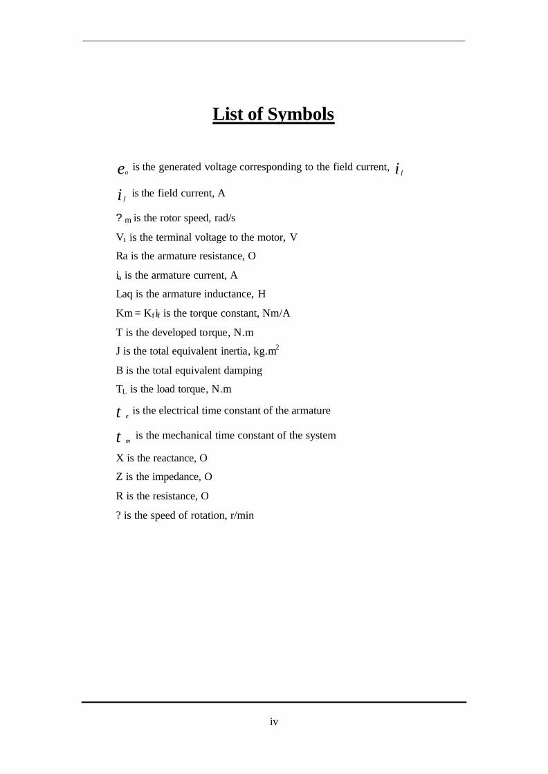
List of Symbols
ea is the generated voltage corresponding to the field current, i f
i f is the field current, A
? m is the rotor speed, rad/s
Vt is the terminal voltage to the motor, V
Ra is the armature resistance, O
ia is the armature current, A
Laq is the armature inductance, H
Km = Kf if is the torque constant, Nm/A
T is the developed torque, N.m
J is the total equivalent inertia, kg.m2
B is the total equivalent damping
TL is the load torque, N.m
τ e is the electrical time constant of the armature
τ m is the mechanical time constant of the system
X is the reactance, O
Z is the impedance, O
R is the resistance, O
? is the speed of rotation, r/min
v
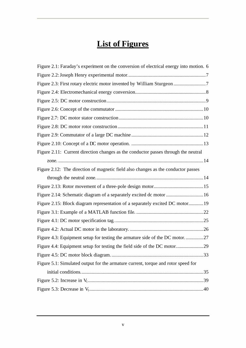
List of Figures
Figure 2.1: Faraday’s experiment on the conversion of electrical energy into motion. 6
Figure 2.2: Joseph Henry experimental motor...............................................................7
Figure 2.3: First rotary electric motor invented by William Sturgeon ..........................7
Figure 2.4: Electromechanical energy conversion.........................................................8
Figure 2.5: DC motor construction................................................................................9
Figure 2.6: Concept of the commutator .......................................................................10
Figure 2.7: DC motor stator construction ....................................................................10
Figure 2.8: DC motor rotor construction .....................................................................11
Figure 2.9: Commutator of a large DC machine ..........................................................12
Figure 2.10: Concept of a DC motor operation. ..........................................................13
Figure 2.11: Current direction changes as the conductor passes through the neutral
zone. .....................................................................................................................14
Figure 2.12: The direction of magnetic field also changes as the conductor passes
through the neutral zone.......................................................................................14
Figure 2.13: Rotor movement of a three-pole design motor........................................15
Figure 2.14: Schematic diagram of a separately excited dc motor ..............................16
Figure 2.15: Block diagram representation of a separately excited DC motor............19
Figure 3.1: Example of a MATLAB function file. ......................................................22
Figure 4.1: DC motor specification tag. .......................................................................25
Figure 4.2: Actual DC motor in the laboratory. ...........................................................26
Figure 4.3: Equipment setup for testing the armature side of the DC motor. ..............27
Figure 4.4: Equipment setup for testing the field side of the DC motor......................29
Figure 4.5: DC motor block diagram. ..........................................................................33
Figure 5.1: Simulated output for the armature current, torque and rotor speed for
initial conditions...................................................................................................35
Figure 5.2: Increase in Vt .............................................................................................39
Figure 5.3: Decrease in Vt............................................................................................40
vi
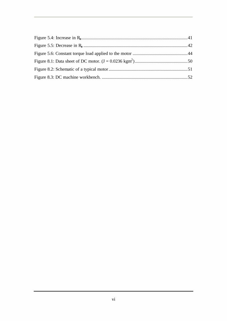
Figure 5.4: Increase in Ra.............................................................................................41
Figure 5.5: Decrease in Ra ...........................................................................................42
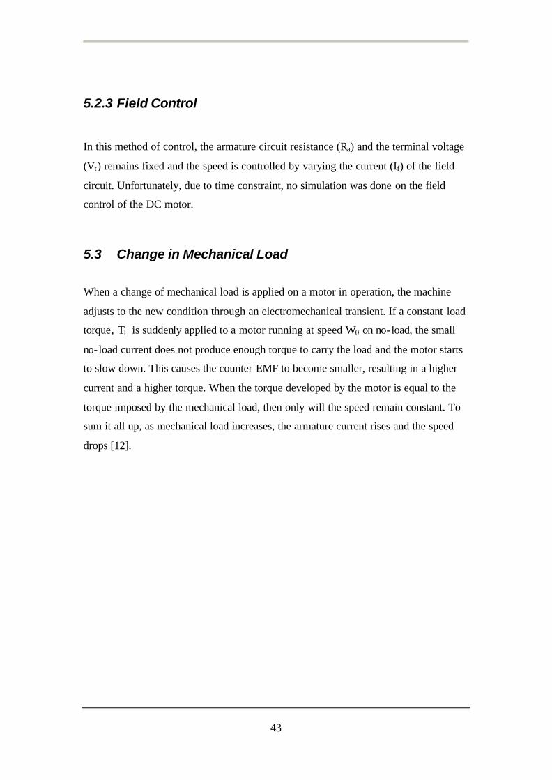
Figure 5.6: Constant torque load applied to the motor ................................................44
Figure 8.1: Data sheet of DC motor. (J = 0.0236 kgm2) ..............................................50
Figure 8.2: Schematic of a typical motor .....................................................................51
Figure 8.3: DC machine workbench. ...........................................................................52
vii
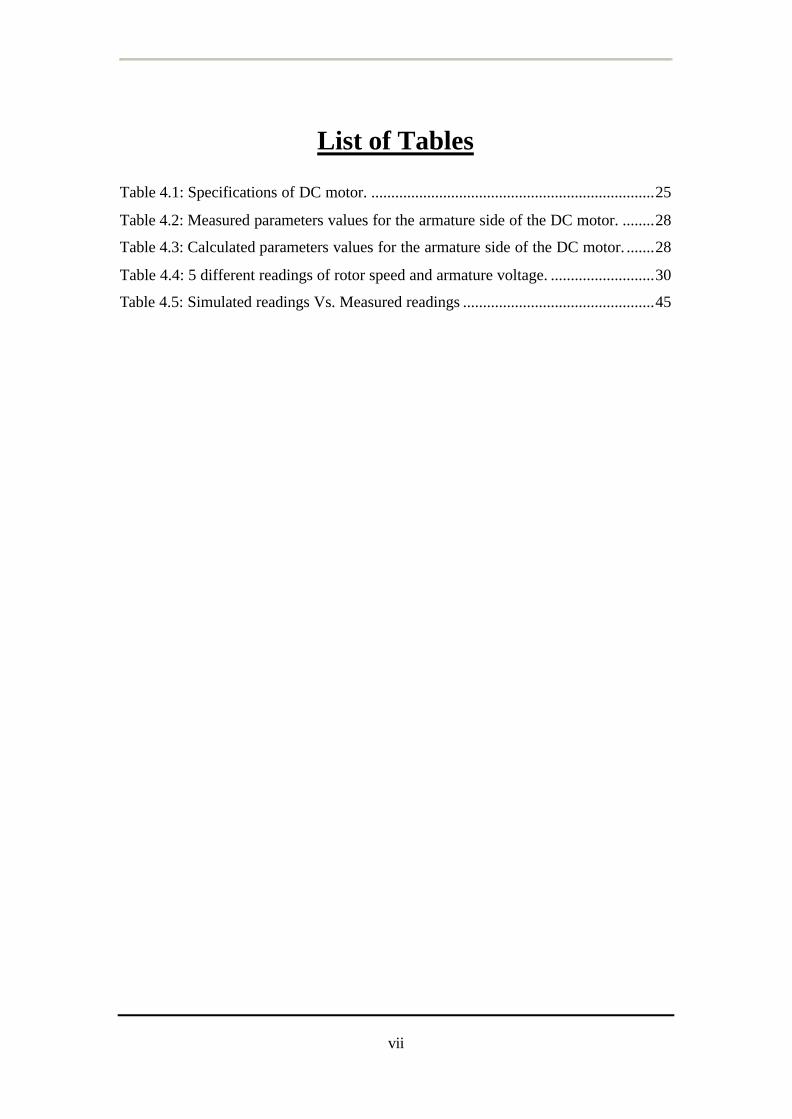
List of Tables
Table 4.1: Specifications of DC motor. .......................................................................25
Table 4.2: Measured parameters values for the armature side of the DC motor. ........28
Table 4.3: Calculated parameters values for the armature side of the DC motor. .......28
Table 4.4: 5 different readings of rotor speed and armature voltage. ..........................30
Table 4.5: Simulated readings Vs. Measured readings ................................................45
viii
Table of contents
LETTER TO DEAN ....................................................................................................I
ACKNOWLEDGEMENT..........................................................................................II
ABSTRACT............................................................................................................... III
LIST OF SYMBOLS .................................................................................................IV
LIST OF FIGURES ....................................................................................................V
LIST OF TABLES ...................................................................................................VII
TABLE OF CONTENTS .......................................................................................VIII
1 INTRODUCTION....................................................................................................1
1.1 AREA OF THE THESIS.......................................................................................2
1.2 MODELLING AND SIMULATION .......................................................................2
1.3 DC MOTOR/GENERATOR ................................................................................2
1.4 AIM OF THESIS ................................................................................................2
1.5 OVERVIEW OF THESIS ......................................................................................3
2 MACHINE BACKGROUND .................................................................................4
2.1 GENERAL MACHINE BACKGROUND ................................................................4
2.2 HISTORY OF DC MOTOR ..................................................................................5
2.3 CONSTRUCTION OF A DC MOTOR ....................................................................9
2.4 PRINCIPLES OF OPERATION ...........................................................................13
2.5 MOTOR MODELLING AND SIMULATION ........................................................16
3 INTRODUCTION TO MATLAB/SIMULINK ..................................................20
3.1 WHAT IS MATLAB? ....................................................................................20
3.2 WHAT IS SIMULINK?..................................................................................20
3.3 APPLICATION PROGRAMMING INTERFACE ....................................................21
3.3.1 M-File.......................................................................................................21
3.3.1.1 Scripts File .......................................................................................21
ix
3.3.1.2 Functions Files.................................................................................22
4 DESIGN METHOD ...............................................................................................24
4.1 MODELLING ..................................................................................................24
5 SIMULATION AND RESULTS ..........................................................................35
5.1 SIMULATION RESULTS ..................................................................................35
5.2 TORQUE – SPEED CHARACTERISTICS ............................................................36
5.2.1 ARMATURE VOLTAGE CONTROL...................................................................38
5.2.2 ARMATURE RESISTANCE CONTROL ..............................................................41
5.2.3 FIELD CONTROL............................................................................................43
5.3 CHANGE IN MECHANICAL LOAD ...................................................................43
5.4 SIMULATED RESULTS VS MEASURED RESULTS .............................................45
6 CONCLUSION AND FUTURE WORK .............................................................46
6.1 CONCLUSION.................................................................................................46
6.2 FUTURE WORK..............................................................................................47
7 BIBLIOGRAPHY..................................................................................................48
8 APPENDICES ........................................................................................................50
APPENDIX A - DATA SHEET OF DC MOTOR ...............................................................50
APPENDIX B - SCHEMATIC OF A TYPICAL MOTOR ......................................................51
APPENDIX C – DC MACHINE WORKBENCH................................................................52
APPENDIX D – MATLAB TEST PROGRAM ...............................................................53
1
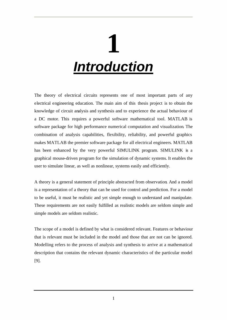
1 Introduction
The theory of electrical circuits represents one of most important parts of any
electrical engineering education. The main aim of this thesis project is to obtain the
knowledge of circuit analysis and synthesis and to experience the actual behaviour of
a DC motor. This requires a powerful software mathematical tool. MATLAB is
software package for high performance numerical computation and visualization. The
combination of analysis capabilities, flexibility, reliability, and powerful graphics
makes MATLAB the premier software package for all electrical engineers. MATLAB
has been enhanced by the very powerful SIMULINK program. SIMULINK is a
graphical mouse-driven program for the simulation of dynamic systems. It enables the
user to simulate linear, as well as nonlinear, systems easily and efficiently.
A theory is a general statement of principle abstracted from observation. And a model
is a representation of a theory that can be used for control and prediction. For a model
to be useful, it must be realistic and yet simple enough to understand and manipulate.
These requirements are not easily fulfilled as realistic models are seldom simple and
simple models are seldom realistic.
The scope of a model is defined by what is considered relevant. Features or behaviour
that is relevant must be included in the model and those that are not can be ignored.
Modelling refers to the process of analysis and synthesis to arrive at a mathematical
description that contains the relevant dynamic characteristics of the particular model
[9].
2
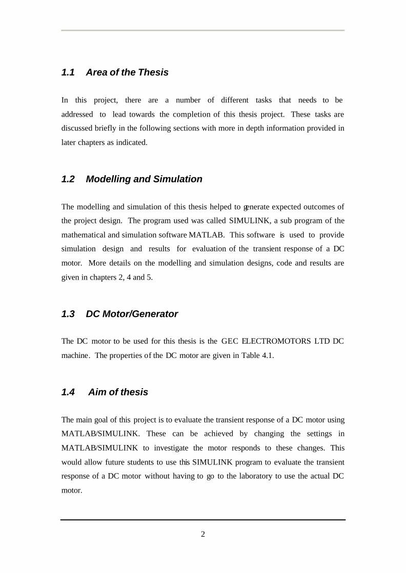
1.1 Area of the Thesis
In this project, there are a number of different tasks that needs to be
addressed to lead towards the completion of this thesis project. These tasks are
discussed briefly in the following sections with more in depth information provided in
later chapters as indicated.
1.2 Modelling and Simulation
The modelling and simulation of this thesis helped to generate expected outcomes of
the project design. The program used was called SIMULINK, a sub program of the
mathematical and simulation software MATLAB. This software is used to provide
simulation design and results for evaluation of the transient response of a DC
motor. More details on the modelling and simulation designs, code and results are
given in chapters 2, 4 and 5.
1.3 DC Motor/Generator
The DC motor to be used for this thesis is the GEC ELECTROMOTORS LTD DC
machine. The properties of the DC motor are given in Table 4.1.
1.4 Aim of thesis
The main goal of this project is to evaluate the transient response of a DC motor using
MATLAB/SIMULINK. These can be achieved by changing the settings in
MATLAB/SIMULINK to investigate the motor responds to these changes. This
would allow future students to use this SIMULINK program to evaluate the transient
response of a DC motor without having to go to the laboratory to use the actual DC
motor.
3
1.5 Overview of thesis
The structure of this thesis is set out into six sections.
• Chapter 1 gives an introduction to this thesis and a brief description of
the different areas that make up the project.
• Chapter 2 will focus on the history, construction and principles of
operation of the DC motor. The implementation of the motor and
software used for the project is also discussed.
• Chapter 3 will introduce the reader to MATLAB/SIMULINK
• Chapter 4 will focus on the modelling of the DC motor using
MATLAB/SIMULINK.
• Chapter 5 reveals the results obtained and gives an analysis of
the outcome of the project, including simulation and practical data.
• Chapter 6 gives a summary and conclusions of the project and suggests
future work that could be done to expand on the final design specified
in this thesis
.
4
2 Machine Background
2.1 General Machine Background
In today’s world, almost all land-based electrical power supply networks are AC
systems of generation, transformation, transmission and distribution. Thus there is
little need for large DC generators. Furthermore, AC motors are used in industries
wherever they are suitable or can give appropriate characteristics by means of power
electronic devices. Yet there remain important fields of application when the DC
machines can offer economic and technical advantage. The wonderful thing about DC
machines is its versatility.
A DC machine can operate as either a generator or a motor but at present its use as a
generator is limited because of the widespread use of AC power. Large DC motors are
used in machine tools, printing presses, conveyors, fans, pumps, hoists, cranes, paper
mills, textile mills and so forth. Small DC machines (in fractional horsepower rating)
are used primarily as control devices such as tacho-generators for speed sensing and
servomotors for positioning and tracking.
DC motors still dominate as traction motors used in transit cars and locomotives as
the torque-speed characteristics of DC motor can be varied over a wide range while
retaining high efficiency. The DC machine definitely plays an important role in
industry.
5
2.2 History of DC motor
Electric motors exist to convert electrical energy into mechanical energy. This is done
by two interacting magnetic fields -- one stationary, and another attached to a part that
can move.
DC motors have the potential for very high torque capabilities (although this is
generally a function of the physical size of the motor), are easy to miniaturize, and can
be "throttled" via adjusting their supply voltage. DC motors are also not only the
simplest, but the oldest electric motors.
The basic principles of electromagnetic induction were discovered in the early 1800's
by Oersted, Gauss, and Faraday. In 1819, Hans Christian Oersted and Andie Marie
Ampere discovered that an electric current produces a magnetic field. The next 15
years saw a flurry of cross-Atlantic experimentation and innovation, leading finally to
a simple DC rotary motor. A number of men were involved in the work. Below are 3
of the most famous people to have experimented about DC motor [10].
Michael Faraday (U.K.)
Fabled experimenter Michael Faraday decided to confirm or refute a number of
speculations surrounding Oersted's and Ampere's results. He set to work devising an
experiment to demonstrate whether or not a current-carrying wire produced a circular
magnetic field around it, and in October of 1821, he succeeded in demonstrating this.
Faraday took a dish of mercury and placed a fixed magnet in the middle. Above this,
he dangled a freely moving wire (the free end of the wire was long enough to dip into
the mercury). When he connected a battery to form a circuit, the current-carrying wire
circled around the magnet. Faraday then reversed the setup, this time with a fixed wire
and a dangling magnet. Again the free part circled around the fixed part. This was the
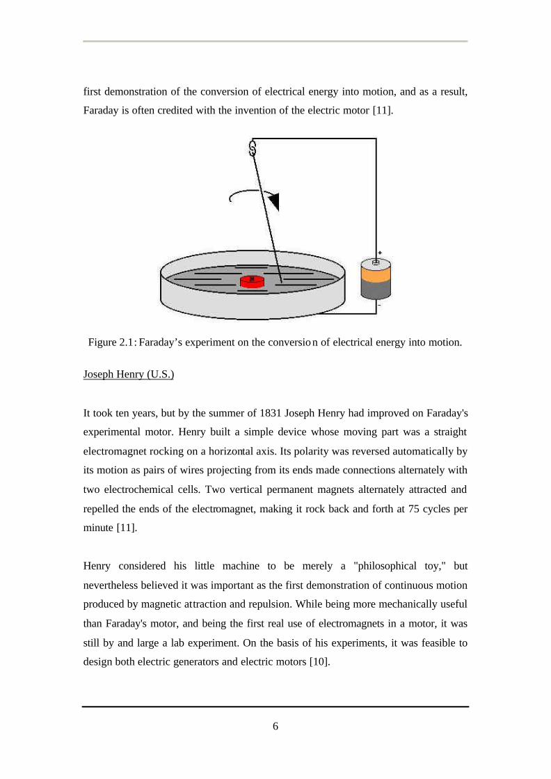
6
first demonstration of the conversion of electrical energy into motion, and as a result,
Faraday is often credited with the invention of the electric motor [11].
Figure 2.1: Faraday’s experiment on the conversion of electrical energy into motion.
Joseph Henry (U.S.)
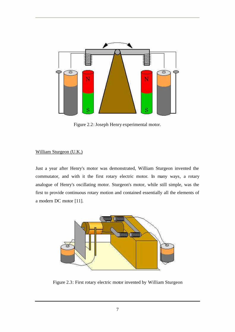
It took ten years, but by the summer of 1831 Joseph Henry had improved on Faraday's
experimental motor. Henry built a simple device whose moving part was a straight
electromagnet rocking on a horizontal axis. Its polarity was reversed automatically by
its motion as pairs of wires projecting from its ends made connections alternately with
two electrochemical cells. Two vertical permanent magnets alternately attracted and
repelled the ends of the electromagnet, making it rock back and forth at 75 cycles per
minute [11].
Henry considered his little machine to be merely a "philosophical toy," but
nevertheless believed it was important as the first demonstration of continuous motion
produced by magnetic attraction and repulsion. While being more mechanically useful
than Faraday's motor, and being the first real use of electromagnets in a motor, it was
still by and large a lab experiment. On the basis of his experiments, it was feasible to
design both electric generators and electric motors [10].
7
Figure 2.2: Joseph Henry experimental motor.
William Sturgeon (U.K.)
Just a year after Henry's motor was demonstrated, William Sturgeon invented the
commutator, and with it the first rotary electric motor. In many ways, a rotary
analogue of Henry's oscillating motor. Sturgeon's motor, while still simple, was the
first to provide continuous rotary motion and contained essentially all the elements of
a modern DC motor [11].
Figure 2.3: First rotary electric motor invented by William Sturgeon
8
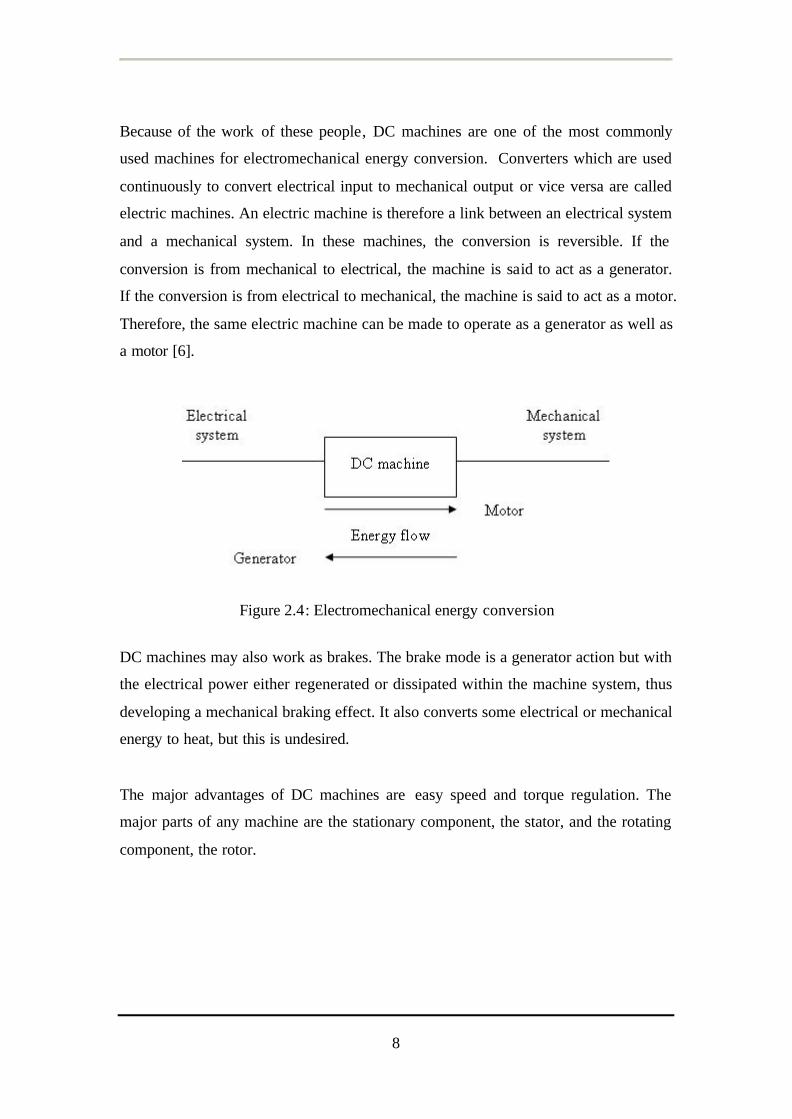
Because of the work of these people, DC machines are one of the most commonly
used machines for electromechanical energy conversion. Converters which are used
continuously to convert electrical input to mechanical output or vice versa are called
electric machines. An electric machine is therefore a link between an electrical system
and a mechanical system. In these machines, the conversion is reversible. If the
conversion is from mechanical to electrical, the machine is said to act as a generator.
If the conversion is from electrical to mechanical, the machine is said to act as a motor.
Therefore, the same electric machine can be made to operate as a generator as well as
a motor [6].
Figure 2.4: Electromechanical energy conversion
DC machines may also work as brakes. The brake mode is a generator action but with
the electrical power either regenerated or dissipated within the machine system, thus
developing a mechanical braking effect. It also converts some electrical or mechanical
energy to heat, but this is undesired.
The major advantages of DC machines are easy speed and torque regulation. The
major parts of any machine are the stationary component, the stator, and the rotating
component, the rotor.
9
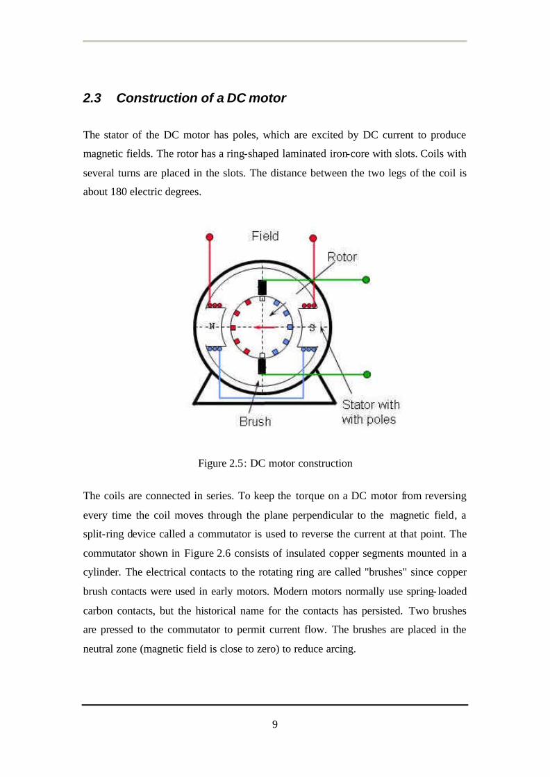
2.3 Construction of a DC motor
The stator of the DC motor has poles, which are excited by DC current to produce
magnetic fields. The rotor has a ring-shaped laminated iron-core with slots. Coils with
several turns are placed in the slots. The distance between the two legs of the coil is
about 180 electric degrees.
Figure 2.5: DC motor construction
The coils are connected in series. To keep the torque on a DC motor from reversing
every time the coil moves through the plane perpendicular to the magnetic field, a
split-ring device called a commutator is used to reverse the current at that point. The
commutator shown in Figure 2.6 consists of insulated copper segments mounted in a
cylinder. The electrical contacts to the rotating ring are called "brushes" since copper
brush contacts were used in early motors. Modern motors normally use spring- loaded
carbon contacts, but the historical name for the contacts has persisted. Two brushes
are pressed to the commutator to permit current flow. The brushes are placed in the
neutral zone (magnetic field is close to zero) to reduce arcing.
10
Figure 2.6: Concept of the commutator
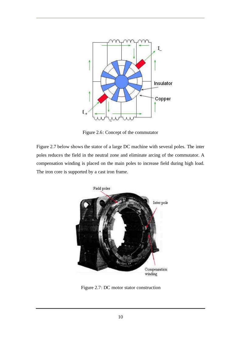
Figure 2.7 below shows the stator of a large DC machine with several poles. The inter
poles reduces the field in the neutral zone and eliminate arcing of the commutator. A
compensation winding is placed on the main poles to increase field during high load.
The iron core is supported by a cast iron frame.
Figure 2.7: DC motor stator construction
11
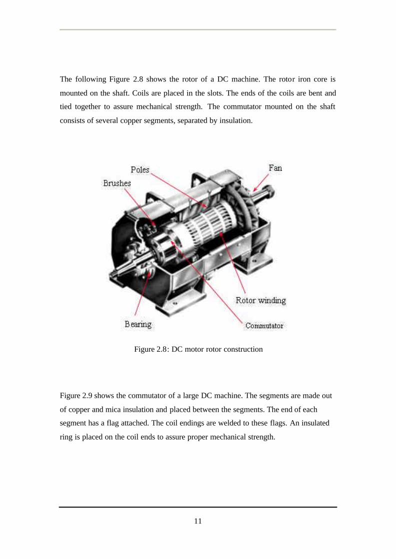
The following Figure 2.8 shows the rotor of a DC machine. The rotor iron core is
mounted on the shaft. Coils are placed in the slots. The ends of the coils are bent and
tied together to assure mechanical strength. The commutator mounted on the shaft
consists of several copper segments, separated by insulation.
Figure 2.8: DC motor rotor construction
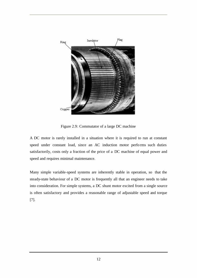
Figure 2.9 shows the commutator of a large DC machine. The segments are made out
of copper and mica insulation and placed between the segments. The end of each
segment has a flag attached. The coil endings are welded to these flags. An insulated
ring is placed on the coil ends to assure proper mechanical strength.
12
Figure 2.9: Commutator of a large DC machine
A DC motor is rarely installed in a situation where it is required to run at constant
speed under constant load, since an AC induction motor perfo rms such duties
satisfactorily, costs only a fraction of the price of a DC machine of equal power and
speed and requires minimal maintenance.
Many simple variable-speed systems are inherently stable in operation, so that the
steady-state behaviour of a DC motor is frequently all that an engineer needs to take
into consideration. For simple systems, a DC shunt motor excited from a single source
is often satisfactory and provides a reasonable range of adjustable speed and torque
[7].
13
2.4 Principles of Operation
In any electric motor, operation is based on simple electromagnetism. A current-
carrying conductor generates a magnetic field which when placed in an external
magnetic field, it will experience a force proportiona l to the current in the conductor
and to the strength of the external magnetic field. The internal configuration of a DC
motor is designed to harness the magnetic interaction between a current-carrying
conductor and an external magnetic field to generate rotational motion.
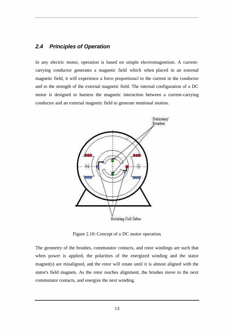
Figure 2.10: Concept of a DC motor operation.
The geometry of the brushes, commutator contacts, and rotor windings are such that
when power is applied, the polarities of the energized winding and the stator
magnet(s) are misaligned, and the rotor will rotate until it is almost aligned with the
stator's field magnets. As the rotor reaches alignment, the brushes move to the next
commutator contacts, and energize the next winding.
14
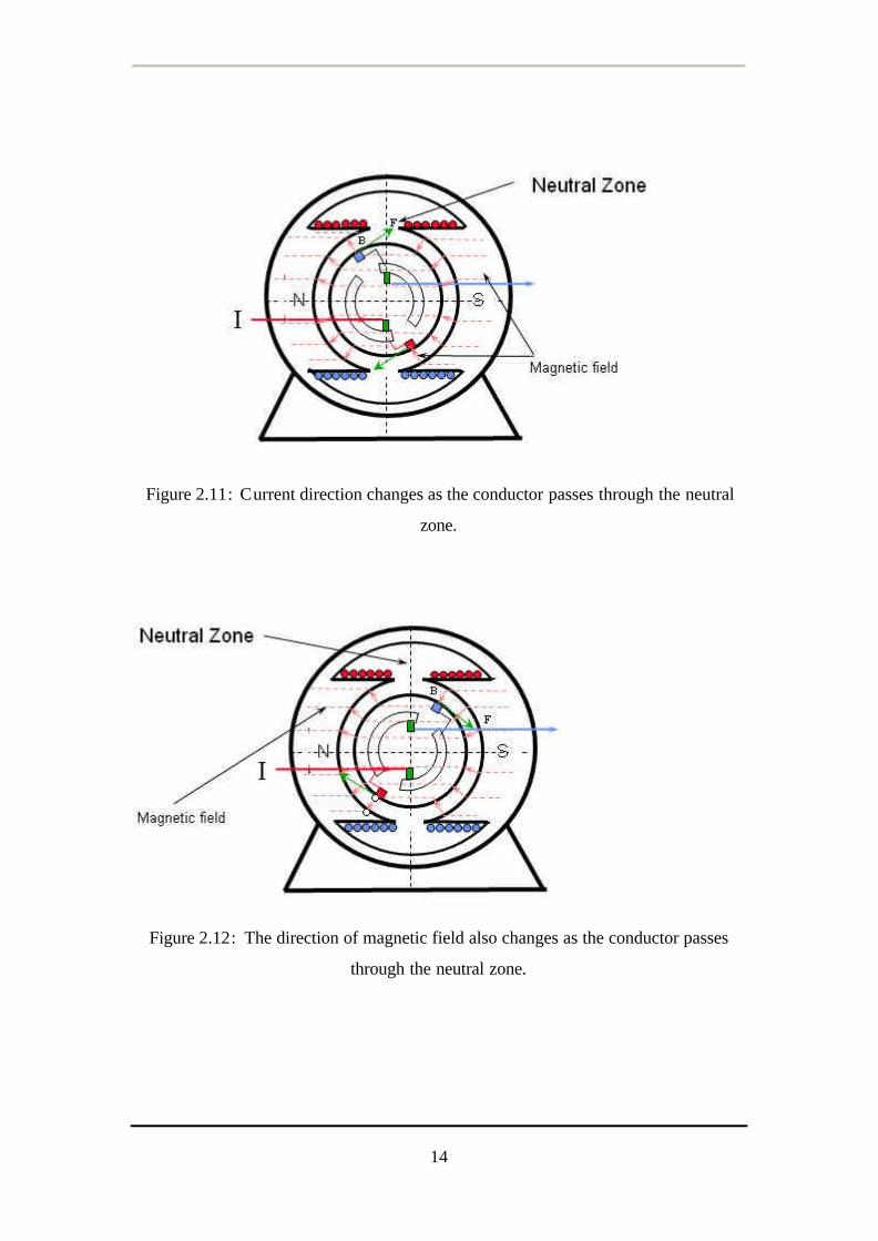
Figure 2.11: Current direction changes as the conductor passes through the neutral
zone.
Figure 2.12: The direction of magnetic field also changes as the conductor passes
through the neutral zone.
15
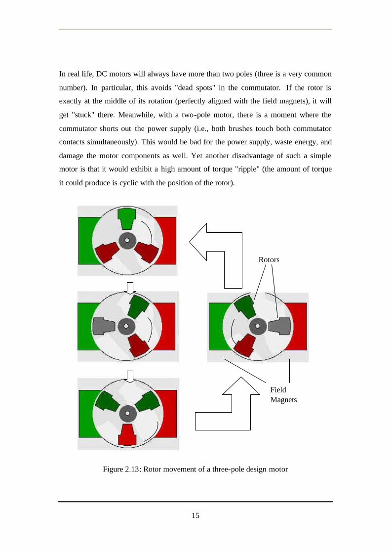
In real life, DC motors will always have more than two poles (three is a very common
number). In particular, this avoids "dead spots" in the commutator. If the rotor is
exactly at the middle of its rotation (perfectly aligned with the field magnets), it will
get "stuck" there. Meanwhile, with a two-pole motor, there is a moment where the
commutator shorts out the power supply (i.e., both brushes touch both commutator
contacts simultaneously). This would be bad for the power supply, waste energy, and
damage the motor components as well. Yet another disadvantage of such a simple
motor is that it would exhibit a high amount of torque "ripple" (the amount of torque
it could produce is cyclic with the position of the rotor).
Figure 2.13: Rotor movement of a three-pole design motor
Field Magnets
Rotors
16
From Figure 2.13, one pole is fully energized at a time (but two others are "partially"
energized). As each brush transitions from one commutator contact to the next, one
coil's field will rapidly collapse, as the next coil's field will rapidly charge up (this
occurs within a few microsecond).
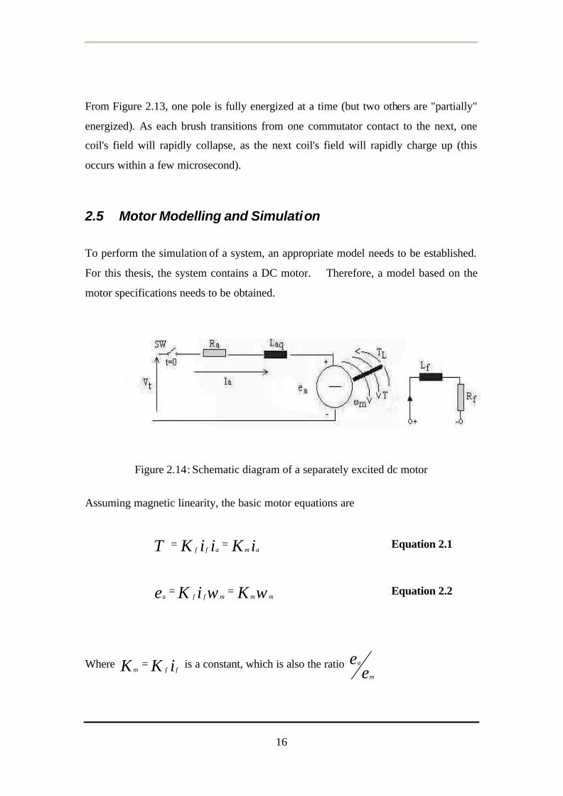
2.5 Motor Modelling and Simulation
To perform the simulation of a system, an appropriate model needs to be established.
For this thesis, the system contains a DC motor. Therefore, a model based on the
motor specifications needs to be obtained.
Figure 2.14: Schematic diagram of a separately excited dc motor
Assuming magnetic linearity, the basic motor equations are
iKiiKT amaff== Equation 2.1
ωω mmmffa KiKe == Equation 2.2
Where iKK ffm= is a constant, which is also the ratio
ee
m
a
17
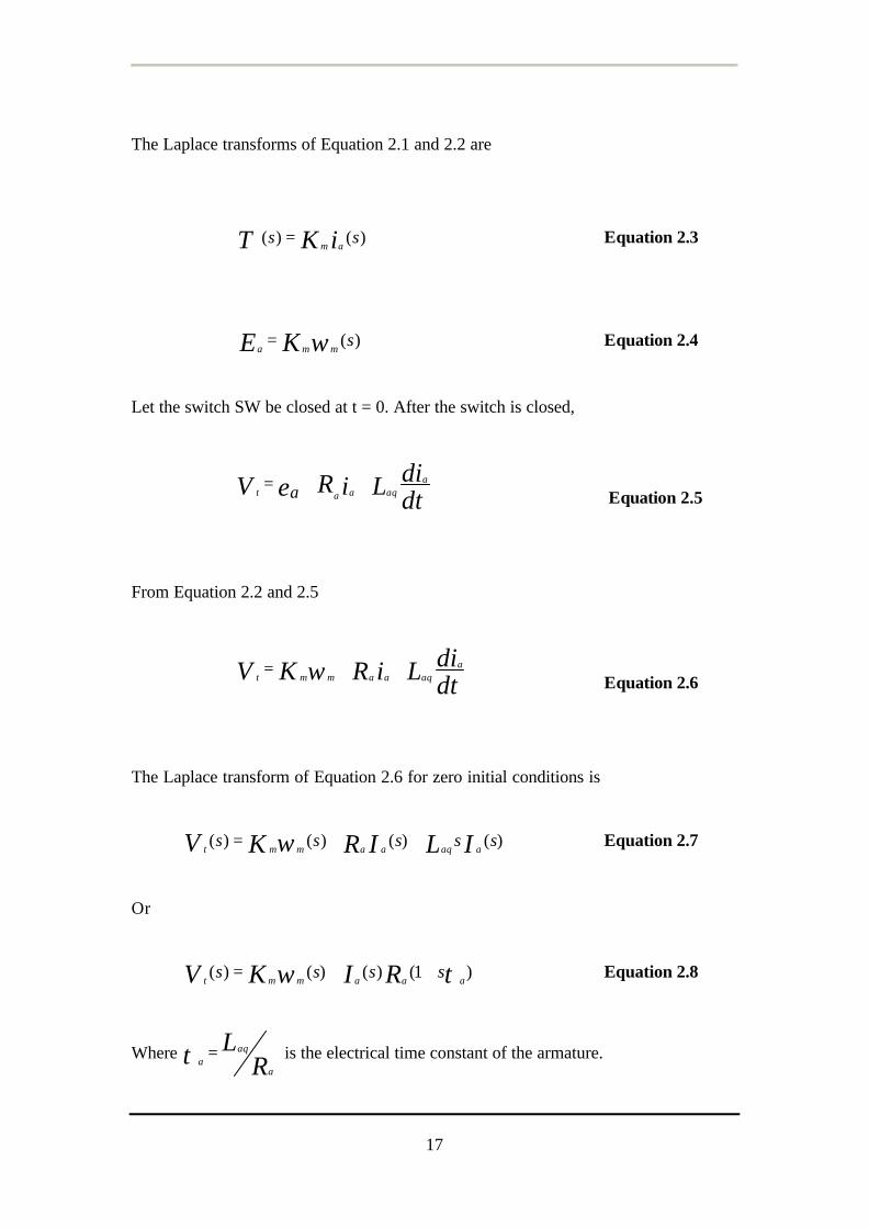
The Laplace transforms of Equation 2.1 and 2.2 are
)()( ss iKT am= Equation 2.3
)(smma KE ω= Equation 2.4
Let the switch SW be closed at t = 0. After the switch is closed,
dtdiLiReV a
aqaat a += + Equation 2.5
From Equation 2.2 and 2.5
dtdiLiRKV a
aqaammt++= ω Equation 2.6
The Laplace transform of Equation 2.6 for zero initial conditions is
)()()()( sssss ILIRKV aaqaammt++= ω Equation 2.7
Or
)1()()()( τω aaammtssss RIKV ++= Equation 2.8
Where R
La
aqa
=τ is the electrical time constant of the armature.
18
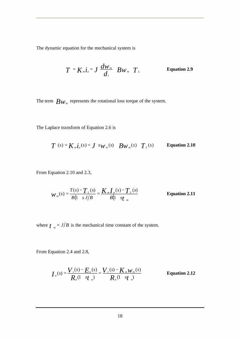
The dynamic equation for the mechanical system is
TBddJiKT Lm
t
mam
++== ωω Equation 2.9
The term ωB m represents the rotational loss torque of the system.
The Laplace transform of Equation 2.6 is
)()()()()( ssssss TBJiKT Lmmam++== ωω Equation 2.10
From Equation 2.10 and 2.3,
( ) ( )τωm
LamLm sB
ss
BJsB
ssTs TIKT
+
−=
+
−=
1
)()(
1
)()()( Equation 2.11
where BJm
=τ is the mechanical time constant of the system.
From Equation 2.4 and 2.8,
)1(
)()(
)1(
)()()(
τω
τ aa
mmt
aa
ata s
ss
s
sss
RKV
REVI +
−=
+
−= Equation 2.12
19
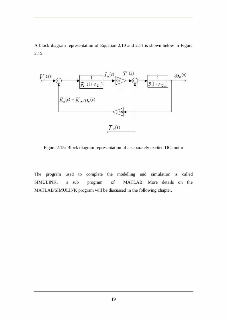
A block diagram representation of Equation 2.10 and 2.11 is shown below in Figure
2.15.
Figure 2.15: Block diagram representation of a separately excited DC motor
The program used to complete the modelling and simulation is called
SIMULINK, a sub program of MATLAB. More details on the
MATLAB/SIMULINK program will be discussed in the following chapter.
20
3 Introduction to
MATLAB/SIMULINK
3.1 What is MATLAB?
The name MATLAB stands for matrix laboratory. MATLAB® is a high-performance
language for technical computing. It integrates computation, visualization, and
programming in an easy-to-use environment where problems and solutions are
expressed in familiar mathematical notation [1].
3.2 What is SIMULINK?
In the last few years, SIMULINK has become the most widely used software package
in academia and industry for modelling and simulating dynamic systems. SIMULINK
is a software package for modelling, simulating, and analysing dynamic systems. It
supports linear and nonlinear systems, modelled in continuous time, sampled time, or
a hybrid of the two. Systems can also be multi-rate, i.e., have different parts that are
sampled or updated at different rates [3].
SIMULINK encourages the user to try things out. User can easily build models from
scratch, or take an existing model and modify it. Simulations are interactive, so user
can change parameters on the spot and immediately see what happens. And because
MATLAB and SIMULINK are incorporated together; user can simulate, analyse, and
revise the models in either environment at any point [3].
21
With SIMULINK, user can move beyond idealized linear models to explore more
realistic nonlinear models, factoring in friction, air resistance, gear slippage, hard
stops, and the other things that describe real-world phenomena. SIMULINK turns the
user computer into a lab for modelling and analysing systems that simply wouldn't be
possible or practical. Be it the behaviour of an automotive clutch system, the flutter of
an airplane wing, the dynamics of a predator-prey model, or the effect of the monetary
supply on the economy [3].
SIMULINK is so practical that thousands of engineers around the world are using it to
model and solve real problems. Knowledge of this software will serve the user well
throughout his/her professional career [3].
3.3 Application Programming Interface
3.3.1 M-File
M-files are normal text files written in MATLAB programming language. The file is
called an M-file because of its file extension of ‘.m’. It allows the user to write a
series of codes into a file and execute them with a single command. The file can be
created using the MATLAB editor or another text editor. There are two types of M-
files, script files and function files, which will be discussed in the following section
[5].
3.3.1.1 Scripts File
The scripts files are the simplest kind of M-file which contains a set of valid
MATLAB commands. The file does not have any input or output arguments and any
variables that they create remain in the workspace, to be used in subsequent
computations. It can be executed by typing the name of the script file excluding the
file extension. It has the same effect of typing all the individual commands stored in
22
the script file at the command line. Script files work on global variables [4]. Therefore
it can operate on existing data in the workspace, or they can create new data on which
to operate [5].
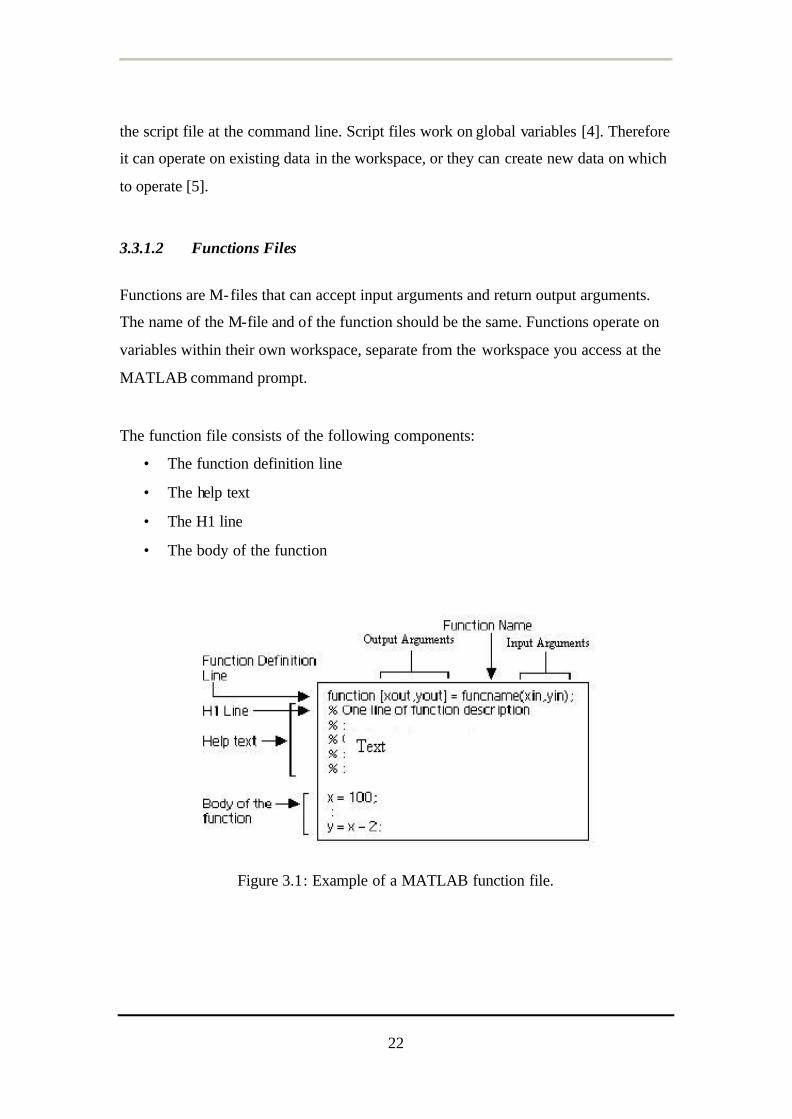
3.3.1.2 Functions Files
Functions are M-files that can accept input arguments and return output arguments.
The name of the M-file and of the function should be the same. Functions operate on
variables within their own workspace, separate from the workspace you access at the
MATLAB command prompt.
The function file consists of the following components:
• The function definition line
• The help text
• The H1 line
• The body of the function
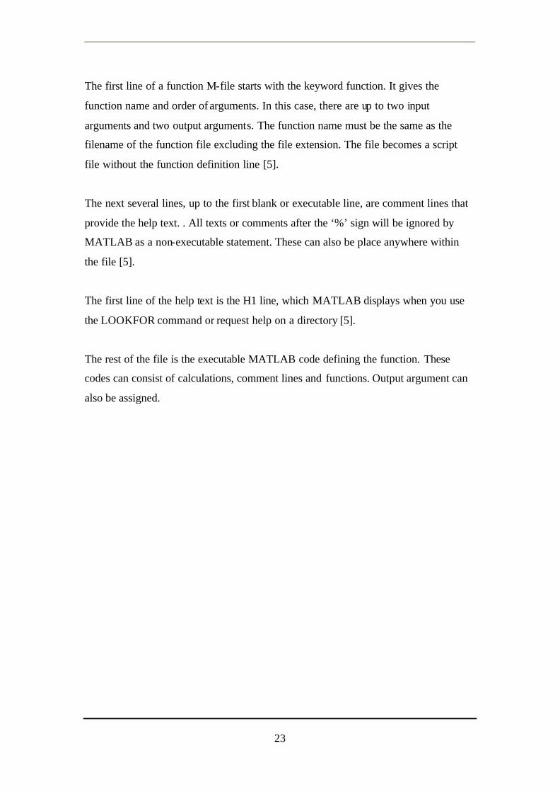
Figure 3.1: Example of a MATLAB function file.
23
The first line of a function M-file starts with the keyword function. It gives the
function name and order of arguments. In this case, there are up to two input
arguments and two output arguments. The function name must be the same as the
filename of the function file excluding the file extension. The file becomes a script
file without the function definition line [5].
The next several lines, up to the first blank or executable line, are comment lines that
provide the help text. . All texts or comments after the ‘%’ sign will be ignored by
MATLAB as a non-executable statement. These can also be place anywhere within
the file [5].
The first line of the help text is the H1 line, which MATLAB displays when you use
the LOOKFOR command or request help on a directory [5].
The rest of the file is the executable MATLAB code defining the function. These
codes can consist of calculations, comment lines and functions. Output argument can
also be assigned.
24
4 Design Method
This thesis involves a number of separate sections, which requires developing
individually and combining to produce the final project. Each part required research
and understanding before being carried out. The design methods used are discussed in
the following sections.
4.1 Modelling
To produce a good design, there needs to be some amount of modelling or simulations
done to avoid aimless trial and error techniques with the actual equipment (the DC
motor).
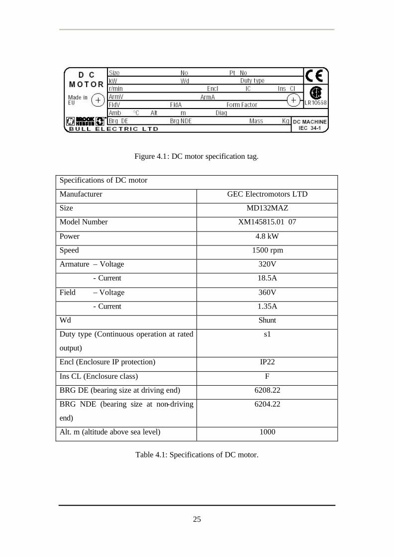
For this thesis project, a number of specifications were needed to be obtained
and established. The specifications of the DC motor were obtained from the
engraving on the metal tag attached onto the motor casing (Figure 4.1). It included the
motor manufacturer company’s name, the size, the model number, power, speed,
voltage and current of the armature and field windings. All of the specifications are
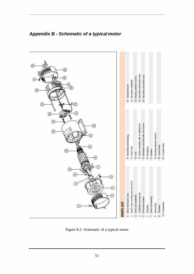
given in Table 4.1. A schematic picture of a typical motor is given in Append ix B.
25
Figure 4.1: DC motor specification tag.
Specifications of DC motor
Manufacturer GEC Electromotors LTD
Size MD132MAZ
Model Number XM145815.01 07
Power 4.8 kW
Speed 1500 rpm
Armature – Voltage 320V
- Current 18.5A
Field – Voltage 360V
- Current 1.35A
Wd Shunt
Duty type (Continuous operation at rated
output)
s1
Encl (Enclosure IP protection) IP22
Ins CL (Enclosure class) F
BRG DE (bearing size at driving end) 6208.22
BRG NDE (bearing size at non-driving
end)
6204.22
Alt. m (altitude above sea level) 1000
Table 4.1: Specifications of DC motor.
26
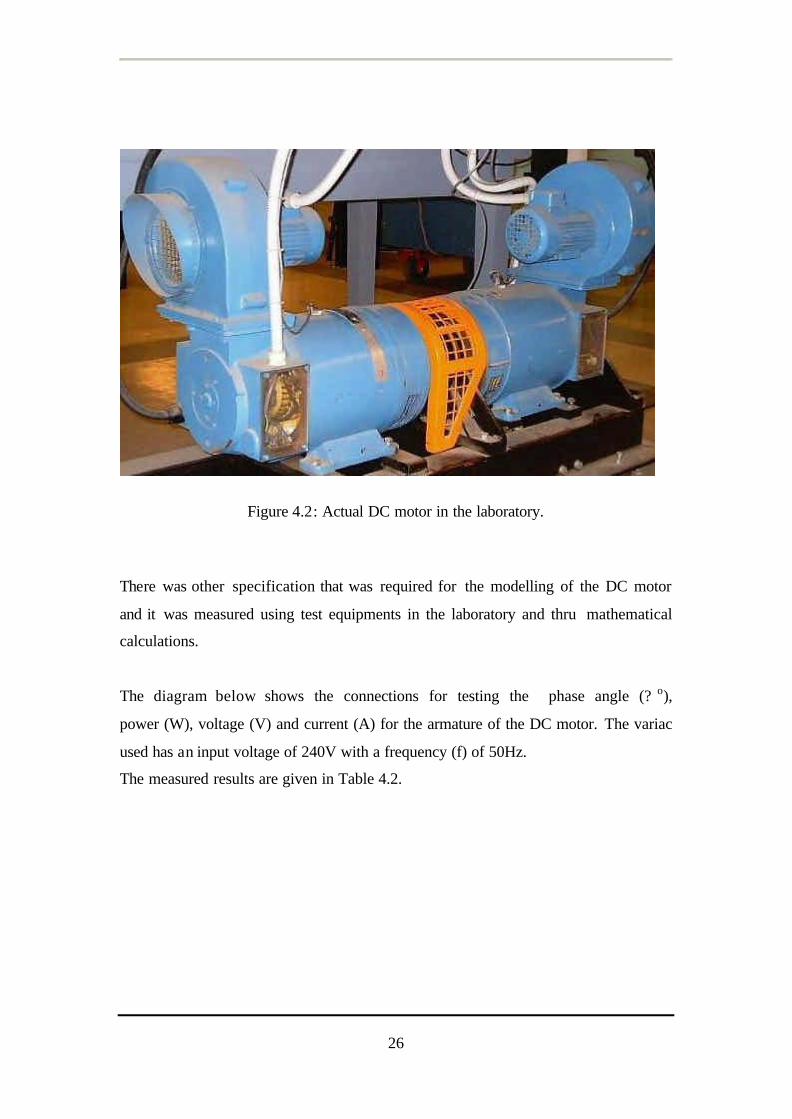
Figure 4.2: Actual DC motor in the laboratory.
There was other specification that was required for the modelling of the DC motor
and it was measured using test equipments in the laboratory and thru mathematical
calculations.
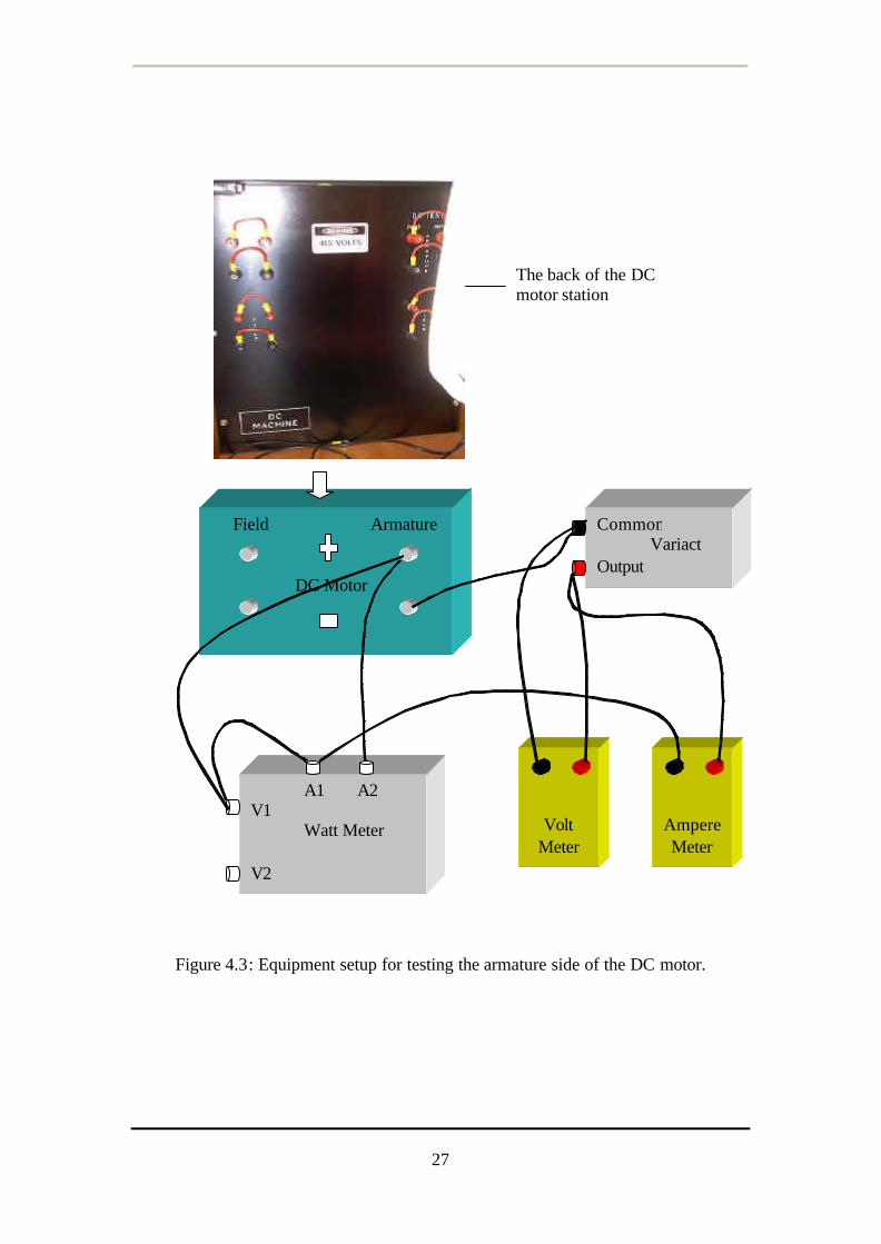
The diagram below shows the connections for testing the phase angle (? o),
power (W), voltage (V) and current (A) for the armature of the DC motor. The variac
used has an input voltage of 240V with a frequency (f) of 50Hz.
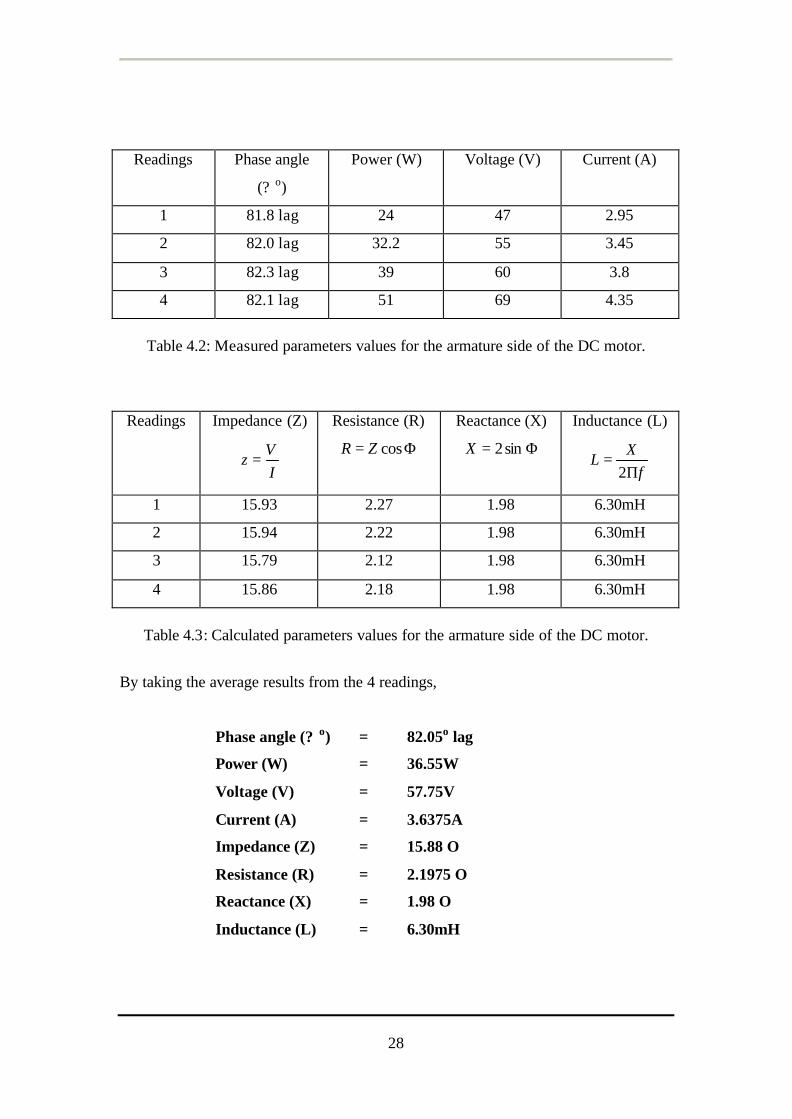
The measured results are given in Table 4.2.
27
Figure 4.3: Equipment setup for testing the armature side of the DC motor.
Field Armature DC Motor
Common Variact Output
A1 A2 V1 Watt Meter V2
Volt Meter
Ampere Meter
The back of the DC motor station
28
Readings Phase angle
(? o)
Power (W) Voltage (V) Current (A)
1 81.8 lag 24 47 2.95
2 82.0 lag 32.2 55 3.45
3 82.3 lag 39 60 3.8
4 82.1 lag 51 69 4.35
Table 4.2: Measured parameters values for the armature side of the DC motor.
Readings Impedance (Z)
IV
z =
Resistance (R)
Φ= cosZR
Reactance (X)
Φ= sin2X
Inductance (L)
fX
LΠ
=2
1 15.93 2.27 1.98 6.30mH
2 15.94 2.22 1.98 6.30mH
3 15.79 2.12 1.98 6.30mH
4 15.86 2.18 1.98 6.30mH
Table 4.3: Calculated parameters values for the armature side of the DC motor.
By taking the average results from the 4 readings,
Phase angle (? o) = 82.05o lag
Power (W) = 36.55W
Voltage (V) = 57.75V
Current (A) = 3.6375A
Impedance (Z) = 15.88 O
Resistance (R) = 2.1975 O
Reactance (X) = 1.98 O
Inductance (L) = 6.30mH
29
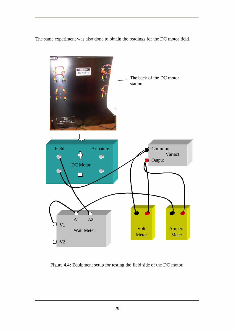
The same experiment was also done to obtain the readings for the DC motor field.
Figure 4.4: Equipment setup for testing the field side of the DC motor.
Field Armature DC Motor
Common Variact Output
A1 A2 V1 Watt Meter V2
Volt Meter
Ampere Meter
The back of the DC motor station
30
However, there were no results to be obtained due to the field having too high
impedance and huge phase change.
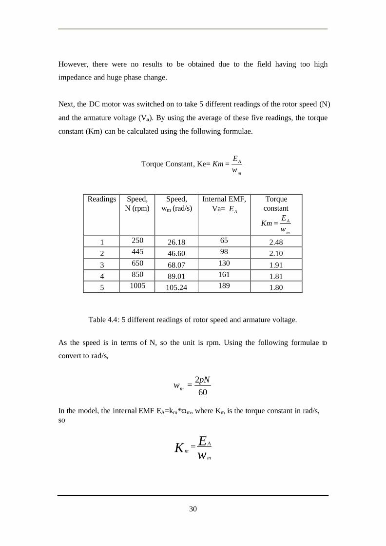
Next, the DC motor was switched on to take 5 different readings of the rotor speed (N)
and the armature voltage (Va). By using the average of these five readings, the torque
constant (Km) can be calculated using the following formulae.
Torque Constant, Ke=m
AEKm
ω=
Readings Speed, N (rpm)
Speed, wm (rad/s)
Internal EMF, Va= AE
Torque constant
m
AEKm
ω=
1 250 26.18 65 2.48 2 445 46.60 98 2.10 3 650 68.07 130 1.91 4 850 89.01 161 1.81 5 1005 105.24 189 1.80
Table 4.4: 5 different readings of rotor speed and armature voltage.
As the speed is in terms of N, so the unit is rpm. Using the following formulae to
convert to rad/s,
602 N
mπω =
In the model, the internal EMF EA=km*ωm, where Km is the torque constant in rad/s, so
ωm
Am
EK =
31
By taking the average results from the above 5 readings,
Torque Constant, Km = 2.02
Looking at the mechanical equation, equation 2.9:
TBddJiK Lm
t
mam
++= ωω
TBiKddJ Lmam
t
m −−= ωω
At steady state both Ia and ωmstabilized,
0=d
dt
mω
So
0=−− TBiK Lmam ω
Since P = 4.8kW, Ia = 18.5A, Km = 1.78, n = 1500rpm
As the speed is in term of N, so the unit is rpm. We need to convert it to rad/s by using
the following formulae.
602 N
mπω =
6015002πω =m
157=mω rad/s
32
Therefore,
WPT L
=
rpmKT L 1500
8.4=
sradT L /1574800=
57.30=T LN.m
Therefore,
(1.78*18.5) – B (157) - TL = 0
32.93 – B (157) – 30.57 = 0
32.93 - 30.57 = B (157)
B = 2.36 / 157
B = 0.015
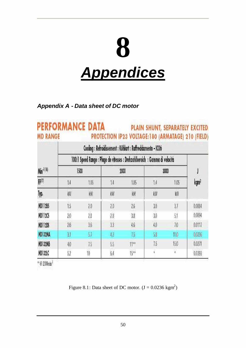
For the value of the rotor inertia J (in kgm2), refer to the data sheet provided in the
Appendix A.
J = 0.0236
With all the required specifications of the DC motor, a model of the DC motor was
developed using SIMULINK. The DC motor was modelled using the characteristics
transfer function of the electrical and mechanical of the motor as shown in Figure 4.5.
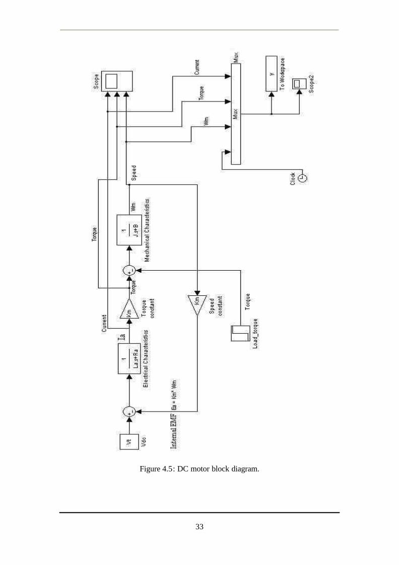
33
Figure 4.5: DC motor block diagram.
34
Figure 4.5 shows the DC motor input armature voltage (Vt) summed with the internal
EMF. The result is then fed into the electrical characteristics transfer function block to
produce the armature current (Ia). It is then pass thru a torque constant to produce
torque. This is then summed with a torque load, giving an output torque which is then
fed into the mechanical characteristics transfer function block. The output is the rotor
speed (Wm), which is fed back into the speed constant providing the constant EMF.
35
5
Simulation and Results
5.1 Simulation Results
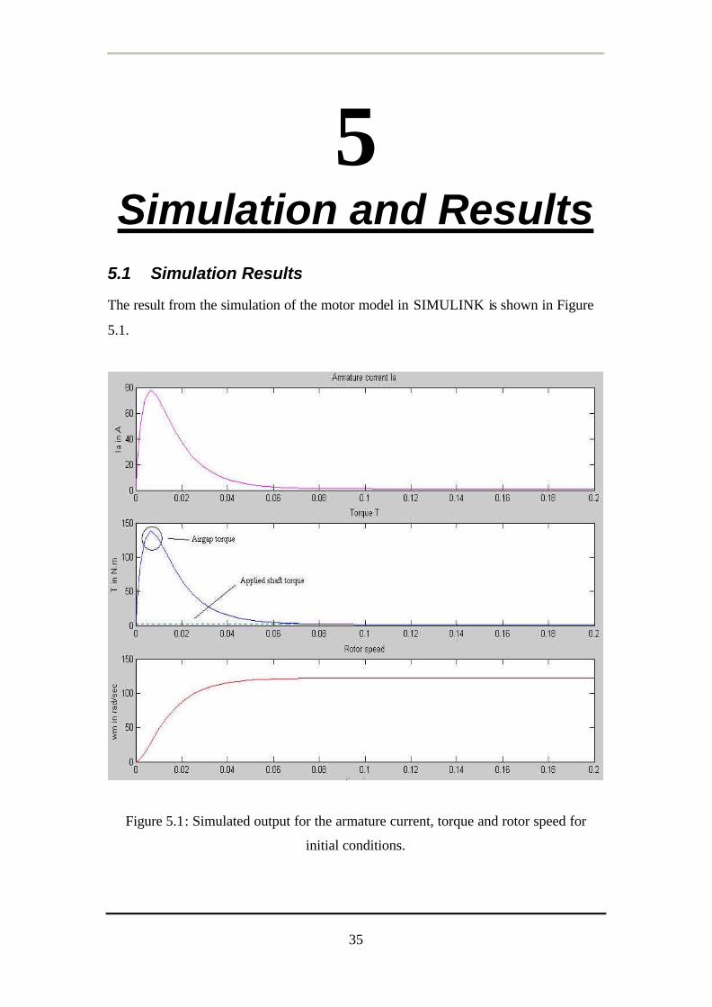
The result from the simulation of the motor model in SIMULINK is shown in Figure
5.1.
Figure 5.1: Simulated output for the armature current, torque and rotor speed for
initial conditions.
36
At standstill, the internal EMF of the armature is zero, but as the rotor speed
increases, the internal EMF will increase along with it. From Figure 5.1, the
simulation result shows that by applying the full- rated voltage to an armature with
low resistance at standstill, it can cause the starting current to reach 20 or more times
its rated value. The advantages of having a direct-on-line (DOL) starting are low cost
and simplicity. However, the large starting current can cause dangerous sparking,
overheating of the armature winding, and increase complexity in operation of the
protection equipment, a large supply voltage drop and a large transient torque which
can damage the mechanical drive train.
5.2 Torque – Speed Characteristics
In many applications, DC motors are used to drive mechanical loads. Some
applications require that the speed remain constant as the mechanical load is applied
to the motor changes. On the other hand, some applications require that the speed be
controlled over a wide range.
The voltage, current, speed and torque are related as follows:
RIVKE aatmaa−== Φ ω Equation 2.12
IKT aa Φ= Equation 2.13
From Equation 2.12, the speed is
Φ
−=
KRIV
a
aatmω Equation 2.14
37
From Equation 2.13 and 2.14,
TKR
KV
a
a
a
tm 2)( ΦΦ
−=ω Equation 2.15
If the terminal voltage (Vt) and machine flux (? ) are kept constant, the drop in speed
as the applied torque increases is small, providing a good speed regulation. In an
actual machine, the flux (? ) will decrease because of armature reaction as T or Ia
increases, and as a result the speed will drop. The armature reaction therefore
improves the speed regulation in a DC motor.
Equation 2.15 suggests that speed control in a DC machine can be achieved by the
following methods:
1. Armature voltage control (Vt).
2. Armature resistance control (Ra).
3. Field control (? ).
Therefore, speed in a DC machine increases as Vt increases and decreases as ? or Ra
increases. The characteristic features of these different methods of speed control of a
DC machine will be discussed further in this chapter [6].
38
5.2.1 Armature Voltage Control
In this method of speed control, the armature circuit resistance (Ra) remains
unchanged and the field current (If) is kept constant (normally at its rated value), and
the armature terminal voltage (Vt) is varied to change the speed. If armature reaction
is neglected, from equation 2.15,
TKVK tm 21−=ω Equation 2.16
Where K1 = 1 / Ka?
K2 = Ra / (Ka? )2
For a constant load torque, the speed will change linearly with (Vt). The armature
voltage control scheme provides a smooth variation of the speed control from zero to
the base speed. The base speed is defined as the speed obtained at rated terminal
voltage. However, this method of speed control is expensive because it requires a
variable DC supply for the armature circuit.
39
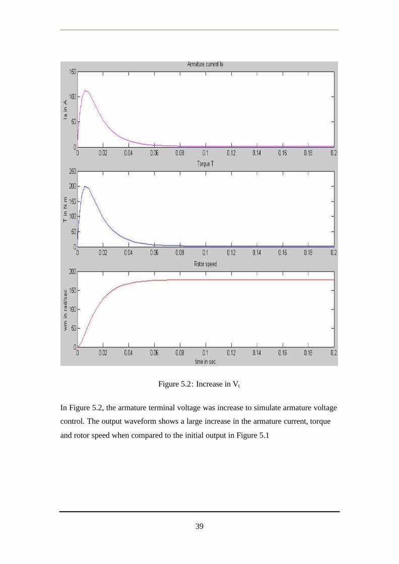
Figure 5.2: Increase in Vt
In Figure 5.2, the armature terminal voltage was increase to simulate armature voltage
control. The output waveform shows a large increase in the armature current, torque
and rotor speed when compared to the initial output in Figure 5.1
40
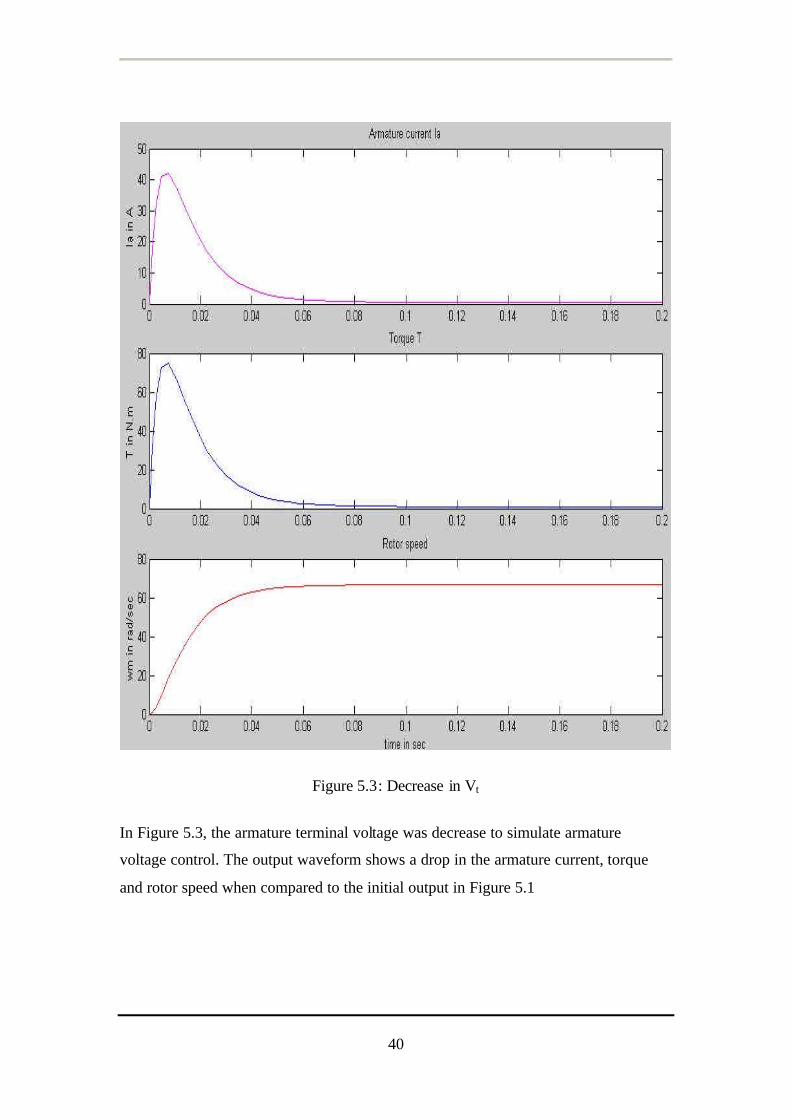
Figure 5.3: Decrease in Vt
In Figure 5.3, the armature terminal voltage was decrease to simulate armature
voltage control. The output waveform shows a drop in the armature current, torque
and rotor speed when compared to the initial output in Figure 5.1
41
5.2.2 Armature Resistance Control
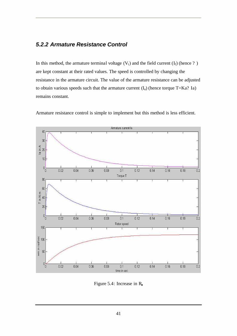
In this method, the armature terminal voltage (Vt) and the field current (If) (hence ? )
are kept constant at their rated values. The speed is controlled by changing the
resistance in the armature circuit. The value of the armature resistance can be adjusted
to obtain various speeds such that the armature current (Ia) (hence torque T=Ka? Ia)
remains constant.
Armature resistance control is simple to implement but this method is less efficient.
Figure 5.4: Increase in Ra
42
From Figure 5.4, the armature resistance was increase to simulate armature resistor
control. The output waveform shows a large drop in the armature current, torque and
rotor speed when compared to the initial output in Figure 5.1. And all the output
waveforms took a longer time to reach steady state.
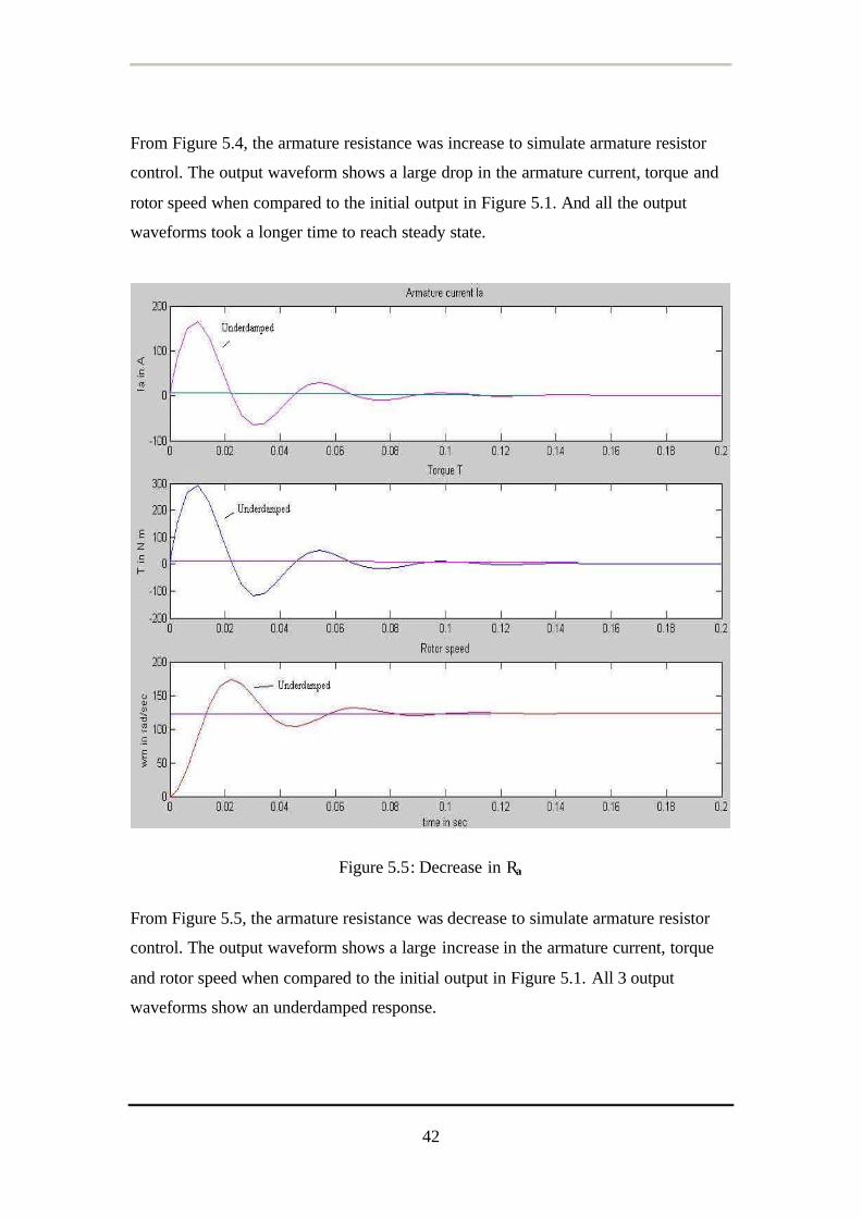
Figure 5.5: Decrease in Ra
From Figure 5.5, the armature resistance was decrease to simulate armature resistor
control. The output waveform shows a large increase in the armature current, torque
and rotor speed when compared to the initial output in Figure 5.1. All 3 output
waveforms show an underdamped response.
43
5.2.3 Field Control
In this method of control, the armature circuit resistance (Ra) and the terminal voltage
(Vt) remains fixed and the speed is controlled by varying the current (If) of the field
circuit. Unfortunately, due to time constraint, no simulation was done on the field
control of the DC motor.
5.3 Change in Mechanical Load
When a change of mechanical load is applied on a motor in operation, the machine
adjusts to the new condition through an electromechanical transient. If a constant load
torque, TL is suddenly applied to a motor running at speed W0 on no- load, the small
no- load current does not produce enough torque to carry the load and the motor starts
to slow down. This causes the counter EMF to become smaller, resulting in a higher
current and a higher torque. When the torque developed by the motor is equal to the
torque imposed by the mechanical load, then only will the speed remain constant. To
sum it all up, as mechanical load increases, the armature current rises and the speed
drops [12].
44
Figure 5.6: Constant torque load applied to the motor
From the simulation results of the DC motor in Figure 5.6, it shows the DC motor
running at no-load condition at start up. After the motor has reached steady-state, if a
mechanical load is suddenly applied to the shaft, the small no- load current does not
produce enough torque to carry the load and the motor begins to slow down. This
causes the counter EMF to diminish, resulting in a higher current and a corresponding
higher torque. When the torque deve loped by the motor is exactly equal to the torque
imposed by the mechanical load, and then the speed will remain constant.
45
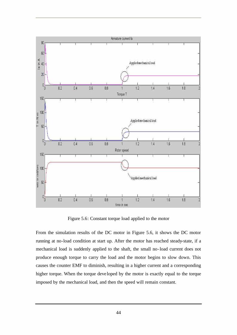
5.4 Simulated results Vs Measured results
Different torque values were loaded into the block diagram and simulated to get the
following. Tests were also done on the actual DC motor using a workbench to get the
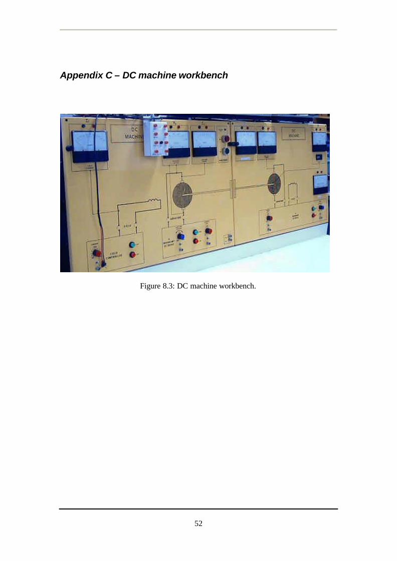
armature current, torque and rotor speed readings. Refer to Appendix C for the picture
of the workbench. The results were placed into Table 4.5.
Simulated Measured Torque
Load,
N.m
Armature
Current,
A
Torque,
N.m
Rotor
speed,
rad/s
Armature
Current, A
Torque,
N.m
Rotor
Speed,
rpm
Rotor
speed,
rad/s
3 2.701 4.807 120.3 3 6.8 1138 119.17
5 3.82 6.799 118.9 4 7 1098 114.9
8 5.502 9.794 116.8 5.6 11 1030 107.86
10 6.637 11.81 115.4 6.2 11.1 945 98.96
11 7.162 12.75 114.8 7 14.1 905 94.77
Table 4.5: Simulated readings Vs. Measured readings
From the results, it can be seen that the simulated readings were slightly similar to the
measured readings. The difference could be put down to not having accurate initial
parameters for the simulation.
46
6 Conclusion and Future
Work
6.1 Conclusion
Actual experimentation on bulky power components can be expensive and time-
consuming. But simulation offers a fast and inexpensive means to learn more about
these components.
In this thesis, the block diagram of a DC motor was developed and by using
SIMULINK, a toolbox extension of the MATLAB program, the block diagram was
simulated with expected waveforms output.
Furthermore, by varying certain parameters of the DC motor block diagram, the
output waveform of the simulation would change accordingly. These parameters
include the field current, armature circuit resistance and armature voltage.
The simulation and modelling of the DC motor also gave an inside look of the
expected output when testing the actual DC motor. The results from the simulation
were never likely to occur in real- life condition due to the response times and
condition of the actual motor.
47
6.2 Future Work
There are a number of topics for future work and development related with the
simulation model designed in this thesis. These may include:
• Inserting external resistors into the armature circuit during start up of the
simulation to reduce the large starting current. These resistors can either be
manually or automatically shorted out as the motor accelerates.
• Modifying the block diagram to control the speed of the DC motor by varying
the current (If) of the field circuit. This can be achieved by using a field circuit
rheostat. This would allow the user to observe the effect on the speed response
of the DC motor speed response by varying the field current
48
7 Bibliography
[1] MathWorks. (2001). Introduction to MATLAB. The MathWorks, Inc.
Available:
http://www.mathworks.com/access/helpdesk/help/techdoc/learn_MATLAB/ch
1intro.shtml#12671
[2] MathWorks. (2001). SIMULINK. The MathWorks, Inc. Available:
http://www.mathworks.com/access/helpdesk/help/toolbox/SIMULINK
/SIMULINK.shtml
[3] MathWorks. (2001). What is SIMULINK. The MathWorks, Inc. Available: http://www.mathworks.com/access/helpdesk/help/toolbox/SIMULINK/ug/ug.s
html
[4] MathWorks. (2000). Using MATLAB Version 6. The MathWorks, Inc.
Available:http://www.mathworks.com/access/helpdesk/help/pdf_doc/MATLA
B/using_ml.pdf
[5] The MathWorks. MATLAB Student Version Learning MATLAB 6 (Release
12), 2nd printing, January 2001.
[6] P.C. Sen, Principles of Electric Machines and Power Electronics (2nd
Edition), John Wiley and Sons Inc., 1989
49
[7] G.R. Slemon and A. Straughen, Electric Machines, Addison-Wesley
publishing company, 1982
[8] D. M. Etter, Engineering Problem Solving with MATLAB, Prentice Hall, 1993.
[9] Chee-Mun Ong, Dynamic Simulation of Electric Machinery, Prentice Hall
PTR, 1998.
[10] Peter F.Ryff, David Platnick and Joseph A.Karnas, Electrical Machines and
Transformers, Principles and Applications, Prentice Hall, Inc., 1987.
[11] The Starting Block. All about DC motors. (2001)
http://www.solarbotics.net/starting/200111_dcmotor/200111_dcmotor.html
[12] Theodore Wildi, Electrical Machines, Drives, and Power Systems, Fourth
Edition, Prentice Hall International, Inc., 2000.
50
8 Appendices
Appendix A - Data sheet of DC motor
Figure 8.1: Data sheet of DC motor. (J = 0.0236 kgm2)
51
Appendix B - Schematic of a typical motor
Figure 8.2: Schematic of a typical motor
52
Appendix C – DC machine workbench
Figure 8.3: DC machine workbench.
53
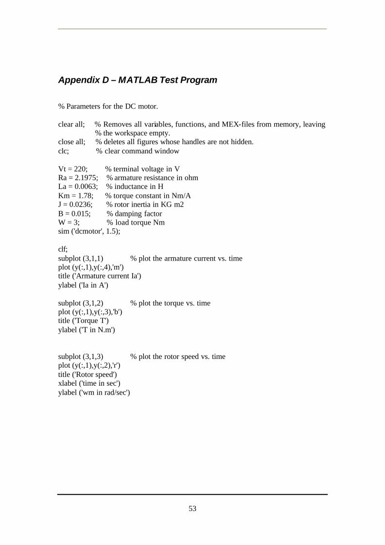
Appendix D – MATLAB Test Program
% Parameters for the DC motor. clear all; % Removes all variables, functions, and MEX-files from memory, leaving % the workspace empty. close all; % deletes all figures whose handles are not hidden. clc; % clear command window Vt = 220; % terminal voltage in V Ra = 2.1975; % armature resistance in ohm La = 0.0063; % inductance in H Km = 1.78; % torque constant in Nm/A J = 0.0236; % rotor inertia in KG m2 B = 0.015; % damping factor W = 3; % load torque Nm sim ('dcmotor', 1.5); clf; subplot (3,1,1) % plot the armature current vs. time plot (y(:,1),y(:,4),'m') title ('Armature current Ia') ylabel ('Ia in A') subplot (3,1,2) % plot the torque vs. time plot (y(:,1),y(:,3),'b') title ('Torque T') ylabel ('T in N.m') subplot (3,1,3) % plot the rotor speed vs. time plot (y(:,1),y(:,2),'r') title ('Rotor speed') xlabel ('time in sec') ylabel ('wm in rad/sec')