MATLAB Software

for Supervised Classification

in Remote Sensing and Image Processing

Johnathan M. Bardsley a, Marylesa Howard a, Mark Lorang b,and Chris Gotschalk c,

aDepartment of Mathematical SciencesUniversity of MontanaMissoula, MT 59812

bFlathead Lake Biological StationUniversity of Montana32125 Bio Station LanePolson, MT 59860-9659cMarine Science InstituteUniversity of California

Santa Barbara, CA, 93106

Abstract

We present MATLAB software for the supervised classification of images. By super-vised we mean that the user has in hand a representative subset of the pixels in theimage of interest. A statistical model is then built from this subset to assign everypixel in the image to a best fit group based on reflectance or spectral similarity. Inremote sensing this approach is typical, and the subset of known pixels is called theground-truth data.

Ideally, a classifier incorporates both spectral and spatial information. In oursoftware, we implement quadratic discriminant analysis (QDA) for spectral clas-sification and a choice of three spatial methods – mode filtering, probability labelrelaxation, and Markov random fields – for the incorporation of spatial context afterthe spectral classification has been computed. Each of these techniques is discussedwith some detail in the text.

Finally, we introduce a graphical-user-interface (GUI) that facilitates the creationof ground-truth data subsets – based on individual pixels, lines of pixels, or polygonsof pixels – that appear to the user to have spectral similarity. Once a ground-truthsubset is created, histogram plots for each band are outputted in order to aid theuser in determining whether to accept or reject it. Therefore the GUI makes thesoftware quantitatively robust, broadly applicable and easily usable. We test ourclassification software on several examples.

Preprint submitted to Environmental Modelling and Software 31 January 2012

Key words: remote sensing, supervised classification, quadratic discriminantanalysis, Markov random fields, probability label relaxation1991 MSC: 68U10, 65C60, 90-08

1 Introduction

Passive remote sensing is the act of making observations from afar of light re-flected from an object. This type of remote sensing data is typically collectedby means of a sensor mounted on an aircraft or spacecraft [1], and collecteddata must be statistically grouped or classified to extract quantitative infor-mation about the object.

Supervised classification refers to a class of methods used in the quantitativeanalysis of remote sensing image data. These methods require that the userprovide the set of cover types in the image—e.g., water, cobble, deciduousforest, etc.—as well as a training field for each cover type. The training fieldtypically corresponds to an area in the image that contains the cover type,and the collection of all training fields is known as the training set or ground-truth data. The ground-truth data is then used to assign each pixel to its mostprobable cover type.

In this paper, we present MATLAB software for the classification of remotelysensed images. Several well-known software packages exist for classifying re-mote sensing imagery, e.g. ArcGIS, however, these packages are expensive andtend to be complicated enough that a GIS specialist is required for their use.One of our primary goals in this work is to provide the applied scientist witha few of the most effective, and also cutting edge, classification schemes cur-rently available. The software includes spectral-based classification as well asclassifiers that incorporate the spatial correlation within typical images. Thesoftware is also unique in that it allows the user to create ground-truth datafrom a particular image via a graphical user interface (GUI). Finally, the soft-ware makes supervised classification (segmentation) techniques available tothe broader imaging science community, which uses MATLAB extensively.

To test our software, we consider images of river flood plains, which are amongthe most dynamic and threatened ecosystems on the planet [2]. Flood plainsare endangered worldwide because most have been permanently inundated

Email addresses: johnathan.bardsley@umontana.edu (Johnathan M.Bardsley), marylesa.howard@umontana.edu (Marylesa Howard),mark.lorang@umontana.edu (Mark Lorang), gots@lifesci.ucsb.edu (ChrisGotschalk).

2

by reservoirs which also reduce geomorphic forming flows or are disconnectedby dikes and armored by bank stabilization structures [3]. River ecosystemsare in a state of constant change, both on the seasonal and yearly scales, aswell as over the course of decades [4]. Remote sensing of flood plain imageryhas become a valuable tool for conserving and protecting ecosystem goodsand services that are important to human well being through modeling riverdynamics [5,4]. Modeling this change is crucial to river ecologists. In particular,analyzing cover type changes over time allows the river ecologist to addressphysical and ecological questions at scales relevant to large river ecology andmanagement of those ecosystem components. To perform such an analysis, thecollection of remotely sensed images is required, as is the classification of thecollected imagery.

A remotely sensed image contains both spectral and spatial information. Inour approach, we advocate first computing a spectral-based classification us-ing quadratic discriminant analysis (QDA) (also called maximum likelihoodclassification [1]). QDA is popular due to its simplicity and compact trainingprocess [6]. It assumes that the spectral information contained in the pixelswithin each cover type follows a multivariate normal distribution. This distri-butional assumption suggests a natural thresholding method, which the userhas the choice of implementing.

A vast number of other supervised classification schemes exist [7], howeverin [8] it is argued that while advances in the performance of newer methodscontinue to be achieved, it is often the case that the simpler methods, such asQDA, achieve over 90% of the predictive power obtained by the most advancedmethods. Moreover, in the comparison studies of algorithms found in [6], itis shown that the QDA classifier excels over artificial neural networks anddecision trees in design effort, training time, and classification accuracy; andin [9,10] it was shown that although neural/connectionist algorithms makeno assumption on statistical distribution, as does QDA, training time can belengthy and the choice of design architecture is rather complex.

Nonetheless, a major drawback of QDA is that it ignores the spatial arrange-ment of the pixels within an image [11]. The correlation that exists betweenneighboring pixels within an image (see, e.g., [12–14]) should, in many in-stances, be incorporated into a classification scheme [1,15]. The effect of spa-tial autocorrelation and its relation to spatial resolution in an image has beenexplored in remote sensing [16,13,14], but less has been done to directly incor-porate spatial autocorrelation into classification. Methods presented in [16,1]suggest pre-classification filters and neighborhood exploitation methods fordealing with spatial autocorrelation. In this paper, and in our software, wepresent filtering techniques as well as the methods of probabilistic label re-laxation and Markov random fields for spatial-based classification. Each ofthese techniques may or may not reclassify a given pixel based on information

3

about its neighbors. Finally, in order to test the effectiveness of our classifica-tion schemes, we have implemented k-fold cross validation.

This paper is arranged as follows. First, in Section 2, we derive both non-spatial and spatial algorithms for supervised classification and present k-foldcross validation, as well as a technique for thresholding. In Section 3, classifi-cation is carried out on a variety of images using a sampling of the methodsfrom Section 2. A discussion and summary of the methods and the results isgiven in Section 4.

2 Methods

We begin with a presentation our spectral-based classifier, QDA. The spatial-based techniques follow, and then we present a thresholding method, as wellas k-fold cross validation for error assessment.

2.1 Spectral-Based Classification: Quadratic Discriminant Analysis

We begin by letting ωi be the ith of theM spectral classes, or cover types, in theimage to be classified. When considering to which spectral class, or cover type,a particular pixel vector x ∈ Rk belongs, we denote the conditional probabilityof x belonging to ωi by p(ωi|x), for i = 1, . . . ,M . We are interested in thespectral class that attains the greatest probability given x. Thus classificationwill yield x ∈ ωi when

p(ωi|x) > p(ωj|x) for all j 6=i. (1)

It remains to define p(ωi|x), which can be related to the conditional probabilityp(x|ωi) via Bayes’ theorem

p(ωi|x) = p(x|ωi)p(ωi)/p(x), (2)

where p(ωi) is the probability that the ith spectral class occurs in the image;and p(x) is the probability density associated with the spectral vector x overall spectral classes. In Bayes’ terminology, p(ωi) is referred to as the priorprobability and is used to model a priori knowledge.

Substituting (1) into (2), and assuming that p(ωi) is the same for all i, theinequality (1) takes the form

p(x|ωi) > p(x|ωj) for all j 6=i. (3)

4

We assume the probability distributions for the classes are multivariate nor-mal, so that

p(x|ωi) = ((2π)N |Σi|)−1/2 exp(−1

2(x−mi)

′Σ−1i (x−mi)

), (4)

where mi ∈ Rk and Σi ∈ Rk×k are the mean vector and covariance matrix,respectively, of the data in class ωi.

To simplify the above equation, we use the discriminant functions gi (x) de-fined to be the natural logarithm of (3), which preserves the inequality sincethe logarithm is a monotone increasing function. Thus our method classifiesx as an element of ωi when

gi(x) > gj(x) for all j 6=i, (5)

where

gi (x) = − ln |Σi| − (x−mi)′Σ−1

i (x−mi). (6)

From here, a variety of different classifiers can be derived based on assump-tions on the discriminant function and the probability model. However, wehave found quadratic discriminant analysis (QDA) to be both very effective,computationally efficient, as well as straightforward to implement. QDA isgiven by (5), (6), with the mean and covariance in (6) approximated usingthe empirical mean and covariance of the data in ground-truth class i. Theeffective k-nearest neighbor method [7] was not implemented due to its greatercomputational burden.

2.2 Spatial-Based Techniques

In QDA, the classification of a particular pixel does not depend on that of it’sneighbors. In certain instances, it is clear that neighbor information shouldbe taken into account. For instance, in an image containing a river, the pixelsin the “water class” should be distributed in a spatially uniform manner inthe classified image. In order to take into account such prior information,additional techniques are needed.

Four separate approaches were taken for incorporating spatial autocorrela-tion of the remotely sensed data into classification: pre-classification filtering,probabilistic label relaxation, post-classification filtering, and Markov randomFields. Each of the four are described in detail in the following subsections.

5

2.2.1 Pre-classification filtering

Pre-classification filtering can be viewed as a denoising technique (low passfilter) for the image to be classified. The filtering is implemented prior toclassification and hence does not directly incorporate spatial context into theclassification scheme. However, it does impose a degree of homogeneity amongneighboring pixels, increasing the probability that adjacent pixels will be clas-sified into the same spectral class.

It requires a neighborhood matrix. In our implementation, we include a first-,second-, and third-order neighborhood:

N1 =1

8

0 1 0

1 4 1

0 1 0

, N2 =1

16

1 2 1

2 4 2

1 2 1

, N3 =1

36

0 0 1 0 0

0 2 4 2 0

1 4 8 4 1

0 2 4 2 0

0 0 1 0 0

. (7)

Convolution of an image by one of these neighborhood matrices yields a newimage in which each pixel value has been replaced by a weighted average of theneighboring pixels (including itself) of the original image, with the weightinggiven explicitly by the values in the chosen neighborhood matrix. If the neigh-borhood is too large comparative to the degree of spatial autocorrelation, thequantitative distinction between cover types could be lost, so the hope is thatthe neighborhoods used are large enough to incorporate neighboring informa-tion, but not so large that individuality of pixels is lost.

To incorporate pre-classification filtering into the algorithm, the conv2 func-tion in MATLAB is used. Each band of the image was convolved separatelywith the neighborhood matrix and the same size matrix was asked to be re-turned so the buffer placed on the image was not returned as well.

2.2.2 Post-Classification Filtering

To filter post-classification, a classification labeling must first be performed.The classified map is then filtered with a defined neighborhood to develop adegree of spatial context. This is a similar idea to the pre-classification filteringmethod, however, the conv2 function from MATLAB cannot be used in thiscase due to the categorical response of the classified map; e.g., the spectralclasses are not ordered such that a pixel in class 1 is closer in form to a pixel inclass 2 than it is to a pixel in class 5. Thus a weighted average of neighboringpixels will not give us information about the central pixel.

Instead we must filter using a different approach [17]. First, a window size is

6

chosen to define the neighborhood size – in our implementation, we use a 3×3window surrounding the central pixel – and each pixel is relabeled by selectingthe spectral class that occurs most often in the neighborhood window.

To implement this in MATLAB, a 1-pixel buffer was placed around the entireimage by replicating its closest pixel, since it is probable that the boundarypixel’s adjacent pixel is of the same spectral class. The nlfilter function wasthen used on the classified map with the mode function, and the buffer pixelswere removed.

2.2.3 Probabilistic Label Relaxation

While post-classification filtering can be effective, it only uses the classifiedimage to incorporate spatial context. Given that we have the values of the dis-criminant function (and hence the corresponding probabilities), it is temptingto want to use this information as well. Probability label relaxation (PLR) isa technique that uses this information to incorporate spatial homogeneity inthe classification [1].

The PLR algorithm begins with a classification – in our case using QDA – aswell as with the corresponding set of probabilities px(ωi) that pixel x belongsto spectral class ωi. A neighborhood is then defined for x and neighboringpixels are denoted by y. The neighborhood should be large enough that allpixels considered to have spatial correlation with pixel x are included [1]; inour implementation, we simply use the pixels to the left, right, above, andbelow.

A neighborhood function Qx(ωi) is then defined so that all pixels in the neigh-borhood have some influence over the probability of pixel x belonging to ωi.The probabilities defined by px(ωi) are then updated and normalized usingQx(ωi). This is done iteratively so that the PLR algorithm has the form

pk+1x (ωi) =

pkx(ωi)Qkx(ωi)∑

i pkx(ωi)Qk

x(ωi). (8)

It remains to define the neighborhood function Qx. We begin with the com-patibility coefficient defined by the conditional probability pxy(ωi|ωj), i.e. theprobability that ωi is the correct classification of pixel x given that ωj is thecorrect classification for neighboring pixel y. We assume that pxy(ωi|ωj) is in-dependent of location, so that it is only the relative location of y with respectto x, and whether or not it is one of its neighbors, that matters. Then, usingthe previously computed classification, we can compute pxy(ωi|ωj) by lookingat the ratio of occurrences of a pixel x and its neighbors y being classifiedinto ωi and ωj, respectively. A location dependent definition for pxy(ωi|ωj)

7

can also be given, but we do not do that in our implementation.

The probabilities py(ωj), which we have in hand, are then modified via theequation ∑

j

pxy(ωi|ωj)py(ωj). (9)

In the approach for computing pxy(ωi|ωj) mentioned in the previous para-graph, this amounts to simple matrix multiplication. Our neighborhood func-tion is then defined as a spatial average of the values of (9), i.e.

Qx(ωi) =∑ydy

∑j

pxy(ωi|ωj)py(ωj) (10)

where dy are the weights for each neighboring pixel y. Generally the weightswill all be the same – as is the case for us – unless there is prior knowledgeabout stronger spatial autocorrelation in one direction than another.

It is recommended that algorithm (8) be iterated until the probabilities havestabilized. There is no predetermined number of iterations for this processto terminate, though in practice it has been observed that beyond the firstseveral iterations the relaxation process can begin to deteriorate [18]. Richardsmentions that five to ten iterations will typically produce satisfactory results[1].

2.2.4 Markov Random Fields

The neighborhood function used in PLR, though intuitive, can only be justifiedheuristically. Another approach that incorporates spatial context, and that canbe justified mathematically, from a Bayesian viewpoint, is Markov randomfields (MRF).

Suppose the image of interest has pixel data X = x1, . . . ,xN, where N isthe number of pixels. Let ωin denote the ith spectral class of xn. Then the setof class labels for the entire image can be represented as Ω = ωi1, . . . , ωiN,where i can be one of i = 1, . . . ,M . Our task is to compute a random fieldΩ that well-approximates the “true” class labeling Ω∗ of the image underinvestigation.

We now take a Bayesian point of view and assume that Ω is a random arraywith (prior) distribution p(Ω). In this context, Ω is sometimes referred to as arandom field. Through classification, we seek the random field Ω that correctlyidentifies the ground-truth, and thus hopefully correctly identifies the entireimage. For this we maximize the posterior probability p(Ω|X), i.e. from Bayes’theorem we compute

Ω = arg maxΩp(Ω|X) ∝ p(X|Ω)p(Ω).

8

Since spatial autocorrelation typically exists in images, we incorporate it intothe posterior probability. Considering a neighborhood N around a pixel vectorxn, we denote the labels on this neighborhood ωδn, δ ∈ N and our objective isnow to maximize p(ωin|xn, ωδn). Using probability theory we can manipulatethe conditional probability as follows

p(ωin|xn, ωδn) = p(xn, ωδn, ωin)/p(xn, ωδn)

= p(xn|ωδn, ωin)p(ωδn, ωin)/p(xn, ωδn)

= p(xn|ωδn, ωin)p(ωit|ωδn)p(ωδn)/p(xn, ωδn). (11)

To simplify (11), note that p(xn|ωδn, ωin) is the probability distribution of xnconditional on both its labeling as the ith class and its given neighborhoodlabelings ωδn for δ ∈ N . We assume that this conditional distribution is inde-pendent of the neighborhood labelings, i.e., p(xn|ωδn, ωin) = p(xn|ωin). Thenwe also have that the measurement vector xn is independent of its neigh-borhood labeling, and hence, p(xn, ωδn) = p(xn)p(ωδn). Substituting theseexpressions into equation (11) then yields

p(ωin|xn, ωδn) = p(xn|ωin)p(ωit|ωδn)p(ωδn)/p(xn)p(ωδn)

= p(xn|ωin)p(ωit|ωδn)/p(xn)

∝ p(xn|ωin)p(ωit|ωδn).

The conditional prior probability p(ωin|ωδn) is the probability for class i ofpixel n given the neighborhood labels ωδn ∈ N . This conditionality forcesour random fields of labels to be known as Markov Random Fields (MRF).Knowing that we have a MRF gives us the ability to express p(ωit|ωδn) in theform of a Gibbs distribution

p(ωit|ωδn) =1

Ze−U(ωin),

where U(ωin) is based on the Ising model

U(ωin) =∑δn

β[1− δ(ωin, ωδn)].

The term δ(ωin, ωδn) is the Kroneker delta, which takes value 1 if the argu-ments are equal and 0 otherwise. We will take Z = 1 as suggested in [1]. Theparameter β > 0, fixed by the user, controls the neighborhood effect. We cannow take p(xn|ωin) to be given by (4).

Taking the natural log of p(ωin|xn, ωδn), as in our derivation of QDA, yields

9

the discriminant function for classification

gin(xn) = −1

2ln |Σi|−

1

2(xn−mi)

′Σ−1i (xn−mi)−

∑δn

β[1−δ(ωin, ωδn)]. (12)

Here β is sometimes referred to as a regularization parameter, and it must bespecified by the user.

Notice that before the Kroneker delta can be computed in the above MRFdiscriminant function, an initial classification must be computed. We do thisusing the QDA classifier. Thus the MRF discriminant function modifies a givenset of labels based on a neighborhood effect. This process should be iterateduntil there are no further changes in labeling [1]; 5-10 iterations is typicallysufficient.

2.3 Error Assessment

2.3.1 Thresholding

The QDA method can only classify a pixel into one of the originally givenspectral classes. The question arises, what happens if the ground-truth datais incomplete, i.e., there are missing classes? In such cases, it is useful tohave an additional spectral class designed for pixels that, with some degree ofcertainty, do not fit into one of the original spectral classes noted by the user.The technique of thresholding addresses this problem.

Thresholding compares the probability value of p(x|ωi) to a user specifiedthreshold. If the probability value is lower than the threshold, the pixel willbe assigned to a discard class. Thus, thresholding extracts the pixels with alow probability of belonging to any of the training classes and places theminto the discard class.

With thresholding, our classification schema now returns x as an element ofωi when

gi(x) > gj(x) ∀ j 6=i and gi(x) > Ti, (13)

where Ti is the threshold associated with spectral class ωi. It is only when theabove does not hold for any i that x is then classified into the discard class.

To determine Ti, we examine the discriminant function; for QDA, it is givenby (6) and the second inequality in (13) becomes

(x−mi)′Σ−1(x−mi) < −Ti − ln |Σi|. (14)

Assuming x is normally distributed with mean mi and covariance Σi, the left

10

hand side of (14) is known to have a χ2 distribution with k degrees of freedom(recall, x ∈ Rk) [19]. The corresponding χ2

k value can be found using MAT-LAB’s chi2inv function for the desired confidence, yielding a correspondingvalue for Ti.

2.3.2 K-fold Cross Validation

Once a classification has been made, we are interested in how accurately itperformed. Since the image in its entirety is unknown, we look to the ground-truth data. First, the ground-truth data set is partitioned into K approxi-mately equal-sized parts. Remove the first part and set it aside to be used asthe testing set while the remaining K − 1 sets become the adjusted trainingset. The classifier is created with the adjusted training set and is then usedto classify the testing set. For example, if K = 10, this is equivalent to using90% of the ground-truth to classify the remaining 10% of the ground-truth.The classified set is then compared to the ground-truth pixels, respectively,and the percent of misclassified pixels is noted. This process is repeated Ktimes (folds) so that each of the K sets is used exactly once as a testing set.The average percent of misclassified pixels is reported.

The recommended K for K-fold cross validation (CV) is K = 5 or 10 [7].If instead, K is taken to be the total number of ground-truth pixels, N , thisprocess is known as the leave-one-out cross validation method. This is approx-imately unbiased, however it may result in high variance due to the similaritiesbetween the N training sets and can be computationally costly. With K = 5or 10, the variance is lower, but bias may play a role in the error assessment.If the classifier is highly affected by the size of the training set, it will overes-timate the true prediction error [7].

3 Numerical Experiments

We test our algorithms on a variety of images. Since ground classification inremote sensing is the application that motivated this work, we begin withthese types of images.

3.1 Multi-Banded Imagery

The classification methods were tested on two different flood plain images fromQuickbird. The first image is of the Middle Fork of the Flathead River in theNyack flood plain bordering Glacier National Park, Montana (left image in

11

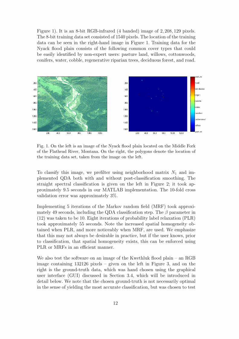
Figure 1). It is an 8-bit RGB-infrared (4 banded) image of 2, 208, 129 pixels.The 8-bit training data set consisted of 1540 pixels. The location of the trainingdata can be seen in the right-hand image in Figure 1. Training data for theNyack flood plain consists of the following common cover types that couldbe easily identified by non-expert users: pasture land, willows, cottonwoods,conifers, water, cobble, regenerative riparian trees, deciduous forest, and road.

Fig. 1. On the left is an image of the Nyack flood plain located on the Middle Forkof the Flathead River, Montana. On the right, the polygons denote the location ofthe training data set, taken from the image on the left.

To classify this image, we prefilter using neighborhood matrix N1 and im-plemented QDA both with and without post-classification smoothing. Thestraight spectral classification is given on the left in Figure 2; it took ap-proximately 9.5 seconds in our MATLAB implementation. The 10-fold crossvalidation error was approximately 3%.

Implementing 5 iterations of the Markov random field (MRF) took approxi-mately 49 seconds, including the QDA classification step. The β parameter in(12) was taken to be 10. Eight iterations of probability label relaxation (PLR)took approximately 55 seconds. Note the increased spatial homogeneity ob-tained when PLR, and more noticeably when MRF, are used. We emphasizethat this may not always be desirable in practice, but if the user knows, priorto classification, that spatial homogeneity exists, this can be enforced usingPLR or MRFs in an efficient manner.

We also test the software on an image of the Kwethluk flood plain – an RGBimage containing 132126 pixels – given on the left in Figure 3, and on theright is the ground-truth data, which was hand chosen using the graphicaluser interface (GUI) discussed in Section 3.4, which will be introduced indetail below. We note that the chosen ground-truth is not necessarily optimalin the sense of yielding the most accurate classification, but was chosen to test

12

Fig. 2. Above is the QDA classification. The lower figures are the classificationsobtained using probability label relaxation (left) and Markov random fields (right),respectively, applied to the QDA classification.

the software.

To classify the image, we implement QDA both with and without post-classificationsmoothing. The straight spectral classification is given on the left in Figure 4;it took approximately 0.32 seconds in our MATLAB implementation. The 10-fold cross validation error was approximately 4.6%. Implementing QDA plus8 iteration of PLR took approximately 1 second. QDA plus 8 MRF iterationswith β = 10 took approximatively 1.8 seconds.

3.2 Thresholding

To use thresholding on the QDA classifier, we must first calculate Ti. Fromequation (14), since the Nyack data set is four-banded, we know the left handside has a χ2 distribution with 4 degrees of freedom. For a 99% acceptancerate, Ti− ln |Σi| = 13.2767 is the value left of which lies 99% of the area underthe χ2 curve with 4 degrees of freedom. Therefore, Ti = −13.2767 − ln |Σi|,

13

Fig. 3. On the left, is an image of a flood plain on the Kwethluk River, Alaska. Onthe right, the polygons denote the location of the training data set, taken from theimage on the left; 1 denotes conifer trees, 2 denotes cobble, 3 denotes water, and 4denotes deciduous trees.

and this is used in equation (14) for classification.

Because the multi-variate Gaussian assumption can be inaccurate for the spec-tral information corresponding to certain cover types, thresholding is not ef-fective in all instances. However, for certain types of problems it is useful. Forexample, suppose that we want to extract the water from the Nyack floodplain image in Figure 1. In this case, it seems unnecessary to ground-truthevery cover type appearing in the given image, since we are not interestedin any cover type other than water. Thus using only water as ground-truthinput, the technique of thresholding at the 99% level was combined with QDAto produce Figure 5. The dark blue on the left image represents the waterthat has been extracted. Ground-truth for the water extraction (light bluepolygons) is displayed in the right image. We created the ground-truth usingthe GUI discussed in Section 3.4. The 10-fold CV error was 0% indicating allof the supplied ground-truth was classified as water and not discarded.

3.3 Classifying General Images

More generally, the software can be used to segment any RGB image – animportant problem in image processing – very efficiently. As an example, con-sider the color image in Figure 6, the ground-truth image obtained using theground-truth GUI of Section 3.4, and the resulting QDA classification thatcannot be improved upon, visually, using a spatial technique such as MRF orPLR. This classification took approximately 2.5 seconds.

Finally, the software can be used on gray-scale and binary images as well fordenoising, which is an important problem in image processing. For our gray-

14

Fig. 4. Above is the QDA classification. The lower figures are the classificationsobtained using probability label relaxation (left) and Markov random fields (right),respectively, applied to the QDA classification.

Fig. 5. Left: River (blue) has been extracted using 99% threshold under QDA. Right:Light blue polygons denote location of water ground-truth from original image

scale example, we use the noisy gray-scale image of Mickey Mouse on the left inFigure 7. For this example, no ground-truth data was used, which is allowed inthe codes provided the mean vectors and the covariance matrices (both scalarsin this case) are provided. For our classification, we chose the five means 1, 90,

15

Fig. 6. On the left is the original RGB image. In the middle is the ground-truthobtained using the GUI; class 4 and 5, corresponding to the basket, are hardlyvisible. On the right is the classification obtained using QDA.

188, 200, and 255, and the variance values were taken to be 1 for every class.The denoising is then accomplished using 10 iteration of the MRF algorithmwith β = 7000, which took approximately 1 second. Implementing the modefiltering, on the other hand, yielded similar results but at approximately 15seconds, a significant increase in computational time.

Fig. 7. On the left is the noisy image of Mickey. The denoised images were obtainedusing MRFs (middle) and mode filtering (right).

Our binary example is given in Figure 8. In this case, the means were takento be 1 and 0, and the variances were both taken to be 1. Ten MRF iterationswith β = 1 yielded the denoised image in the middle in Figure 8 and tookapproximately 2 seconds. On the right in Figure 8 is the denoised image ob-tained using mode filtering, which took approximately 55 seconds to compute.

3.4 Using the Software and Ground-truth GUI

At the web site ‘www.math.umt.edu/bardsley/codes/’ download the zip filenamed ClassifyImages, unzip it and open MATLAB in the resulting direc-tory. Type “startup” at the MATLAB prompt, which adds the directoriesCLASSIFY&TESTS, GUI, and IMAGES to the MATLAB path. The exam-ples above can be reproduced by typing TestNyack, TestKweth, TestMickey,

16

Fig. 8. On the left is the noisy binary image of a Zebra. The denoised images wereobtained using MRFs (middle) and mode filtering (right).

TestHotAirBalloon, or TestZebra at the MATLAB prompt and hitting en-ter. These m-files can be found in the CLASSIFY&TESTS directory and canbe used as a template for the implementation of the code on other problems.

In the files mentioned above, ground-truth images were used that were createdby the authors using the GUI. We now discuss, in detail, how to use theGUI to create your own ground-truth TIFF files. The GUI, coupled with theclassification codes, makes the segmentation of images extremely simple andefficient.

To create ground-truth using the GUI, after following the directions in thefirst two sentences of this section, type RUN GUI at the MATLAB promptand hit enter. The GUI will open in a separate box. First, click the “Load araw tiff” button and choose the image to be classified; it will open as Figure1.

Next, either choose a cover type from the drop down menu labeled “Pickfrom cover type list” or create a new cover type by typing it into the boxlabeled “Add new cover type to list” and then pressing the ENTER key. Ifthe latter was performed, the newly created cover type is now available in thedrop down menu “Pick from cover type list”. Once a cover type is selected,a corresponding color needs to be chosen. Color choices that contrast withthe background image allow the user to more easily locate small cover typeregions.

Ground truth pixels that represent a cover type (e.g. groups of similar trees)are isolated by enclosing within a polygon or by intersecting with a line orpoint. If the image requires being zoomed in to view ground-truth pixels forselection, this adjustment needs to be completed before selecting the preferredbutton for delineating ground-truth. Once the image is at the necessary reso-lution, select the button for method of ground-truthing: “polygon”, “line” or“points”. This brings up cross-hairs on the image. A left click selects verticesto initiate the ground-truth selection process and a right click ends it. Oncethe selection is ended, use a left click to edit vertices or pixels. A double clickends the session for that cover type.

17

Two new figures will open. Figure 2 is a repeated image of Figure 1, thoughFigure 1 now contains delineation of the recently acquired ground-truth. Fig-ure 3 contains a frequency distribution of the recently acquired ground-truthfor each band of data. The ground-truth must be accepted or redone using thecorresponding buttons on the GUI. If “Redo” is chosen, the most recently ac-quired ground-truth is rejected. If “Accept” is chosen, the user has the choiceof generating more ground-truth – either for the same or a different cover type– or of finishing the session by selecting “Save/Exit”. A snapshot of the GUIcan be seen in Figure 9.

Fig. 9. A snapshot of the GUI. On the lower-right are the histograms for each bandof the spectral values for the chosen pixels.

Once the “Save/Exit” button is clicked, the ground-truth is saved in the samedirectory as the original in a *.mat file beginning with the name of the im-age used, then “ GTOutput ”, followed by the date and time. To save theground-truth as an 8-bit *.tif file, first load it into MATLAB with the com-mand “load”, followed by the name of the *.mat file. The command

>> imwrite(output.groundTruth.matrix,’groundtruth.tif’,’tiff’)

writes the ground-truth to the file groundtruth.tif. To call the correspond-ing classes, use the command “output.groundTruth.name”. This ground truthdata can then be used to perform a classification by modifying one of the files

18

mentioned in the first paragraph of this section. Note that this version of theGUI loads only three banded data, so modifications to the number of classesin the above example may need to be made.

4 Conclusions

In this paper, we outline a MATLAB software package for the supervised clas-sification of images. The software uses quadratic discriminant analysis (QDA)for spectral classification and contains three methods for spatial smoothingafter a spectral classification has been computed. These spatial methods in-clude mode filtering, probability label relaxation, and Markov random fields.Also included is a thresholding technique based on the multi-variate Gaussianassumption used in the motivation of QDA, as well as k-fold cross validationfor error analysis.

The software contains a graphical user interface (GUI) that enables the userto generate subsets, known as ground-truth data, for building statistical clas-sifiers. Current versions of MATLAB do not contain such software, hence theuse of the ground-truth GUI is essential in allowing our classification softwareto be widely and easily useable.

The software is tested on a number of images – two examples from remotesensing and three generic images – in order to illustrate its usefulness on abroad range of image processing applications. The examples also show thatthe software is useful, easy to use, and efficient on large-scale problems.

Acknowledgements

Support for PhD student M. Wilde came from an NSF grant to JMB andMSL, Mathematical methods for habitat classification of remote sensing im-agery from river flood plains, NSF-EPSCoR Large River Ecosystems GrantEPS-0701906. Partial support for JMB and MSL came from the Gordon andBetty Moore Foundation (UM grant #344.01) The Salmonid Rivers Obser-vatory Network: Relating Habitat and Quality to Salmon Productivity forPacific Rim Rivers, Stanford PI, Hauer, Kimball, Lorang, Poole Co-PI’s, andsupport for C. Footstalk to write the GUI came from a grant to MSL (UMgrant PPL#443216) from Pennslyviana Power and Light.

19

References

[1] J. Richards, X. Jia, Remote Sensing Digital Analysis, an Introduction, Springer-Verlag, Berlin, 2006.

[2] K. Tockner, J. A. Stanford, Riverine floodplains: present state and future trends,Environmental Conservation 29 (2002) 308–330.

[3] K. Tockner, M. S. Lorang, J. A. Stanford, River flood plains are modelecosystems to test general hydrogeomorphic and ecological concepts, RiverResearch and Applications 26 (2010) 76–86.

[4] J. A. Stanford, M. S. Lorang, F. R. Hauer, The shifting habitat mosaic of riverecosystems, Verh. Internat. Verein. Limnol. 29 (2005) 123–136.

[5] D. W. M.S. Lorang, F. Hauer, J. Kimball, J. Stanford, Using airbornemultispectral imagery to evaluate geomorphic work across floodplains of gravel-bed rivers, Ecological Applications 15 (2005) 1209–1222.

[6] M. Pal, P. Mather, An assessment of the effectiveness of decision tree methodsfor land cover classification, Remote Sensing of the Environment 86 (2003) 554–565.

[7] T. Hastie, R. Tibshirani, J. Friedman, The elements of statistical learning (2001)214–216.

[8] D. J. Hand, Classifier technology and the illusion of progress, Statistical Science21 (1) (2006) 1–14.

[9] G. M. Foody, M. K. Arora, An evaluation of some factors affecting the accuracyof classification by an artificial neural network, International Journal of RemoteSensing 18 (1997) 799–810.

[10] G. G. Wilkinson, Open questions in neuro-computing for earth observation,in: Neuro-Computational in Remote Sensing Data Analysis, Springer-Verlag,Berlin, 1997, pp. 3–13.

[11] S. Tadjudin, D. Landgrebe, Classification of high dimensional data with limitedtraining samples, Tech. Rep. 98-08, Electrical and Computer EngineeringDepartment, Purdue University (1998).

[12] T. G. Congalton, Using spatial autocorrelation analysis to explore the errors inmaps generated from remotely sensed data, Photogrammetric Engineering andRemote Sensing 54 (5) (1988) 587–592.

[13] J. S. Spiker, T. A. Warner, Scale and spatial autocorrelation from a remotesensing perspective, in: Geo-Spatial Technologies in Urban Environments,Springer, Berlin/Heidelberg, Germany, 2007, Ch. 10, pp. 197–213.

[14] S. Yin, X. Chen, Z. Yu, Y. Sun, Y. Cheng, Scale dependence of autocorrelationfrom a remote sensing perspective, Proceedings of SPIE, Geoinformatics 2008and Joint Conference on GIS and Built Environment: Advanced Spatial DataModels and Analyses 7146 (2008) 71461T–1 to 71461T–9.

20

[15] P. Switzer, Extensions of linear discriminant analysis for statistical classificationof remotely sensed satellite imagery, Mathematical Geology 12 (4) (1980) 367–376.

[16] D. M. C. and H. Wei, The effect of spatial autocorrelation and class proportionon the accuracy measures from different sampling designs, ISPRS Journal ofPhotogrammetry and Remote Sensing 64 (2009) 140–150.

[17] F. Townsend, The enhancement of computer classifications by logicalsmoothing, Photogrammetric Engineering and Remote Sensing 52 (1986) 213–221.

[18] J. Richards, D. Landgrebe, P. Swain, On the accuracy of pixel relaxationlabelling, IEEE Transactions on Systems, Man and Cybernetics SMC-6 (1981)420–433.

[19] T. W. Anderson, An Introduction to Multivariate Statistical Analysis, Wiley,New York, 1984.

21