Matlab Kap. III − Images − File-Formate − Advanced Displays

What is the Image Processing Toolbox?

• The Image Processing Toolbox is a collection of functions that extend the capabilities of the MATLAB’s numeric computing environment. The toolbox supports a wide range of image processing operations, including: – Geometric operations – Neighborhood and block operations – Linear filtering and filter design – Transforms – Image analysis and enhancement – Binary image operations – Region of interest operations

Images in MATLAB

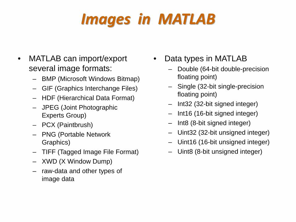
• MATLAB can import/export several image formats:

– BMP (Microsoft Windows Bitmap) – GIF (Graphics Interchange Files) – HDF (Hierarchical Data Format) – JPEG (Joint Photographic

Experts Group) – PCX (Paintbrush) – PNG (Portable Network

Graphics) – TIFF (Tagged Image File Format) – XWD (X Window Dump) – raw-data and other types of

image data

• Data types in MATLAB – Double (64-bit double-precision

floating point) – Single (32-bit single-precision

floating point) – Int32 (32-bit signed integer) – Int16 (16-bit signed integer) – Int8 (8-bit signed integer) – Uint32 (32-bit unsigned integer) – Uint16 (16-bit unsigned integer) – Uint8 (8-bit unsigned integer)

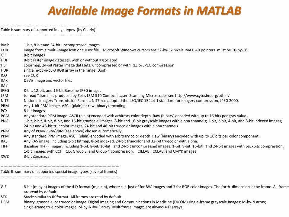
-------------------------------------------------------------------------- Table I: summary of supported image types (by Charly) -------------------------------------------------------------------------- BMP 1-bit, 8-bit and 24-bit uncompressed images CUR image from a multi-image icon or cursor file. Microsoft Windows cursors are 32-by-32 pixels. MATLAB pointers must be 16-by-16. GIF 8-bit images HDF 8-bit raster image datasets, with or without associated H5 colormap; 24-bit raster image datasets; uncompressed or with RLE or JPEG compression HDR single m-by-n-by-3 RGB array in the range [0,inf) ICO see CUR IMX DaVis image and vector files IM7 JPEG 8-bit, 12-bit, and 16-bit Baseline JPEG images LSM to read *.lsm files produced by Zeiss LSM 510 Confocal Laser Scanning Microscopes see http://www.cytosim.org/other/ NITF National Imagery Transmission Format. NITF has adopted the ISO/IEC 15444-1 standard for imagery compression, JPEG 2000. PBM Any 1-bit PBM image, ASCII (plain) or raw (binary) encoding. PCX 8-bit images PGM Any standard PGM image. ASCII (plain) encoded with arbitrary color depth. Raw (binary) encoded with up to 16 bits per gray value. PNG 1-bit, 2-bit, 4-bit, 8-bit, and 16-bit grayscale images; 8-bit and 16-bit grayscale images with alpha channels; 1-bit, 2-bit, 4-bit, and 8-bit indexed images;

24-bit and 48-bit truecolor images; 24-bit and 48-bit truecolor images with alpha channels PNM Any of PPM/PGM/PBM (see above) chosen automatically. PPM Any standard PPM image. ASCII (plain) encoded with arbitrary color depth. Raw (binary) encoded with up to 16 bits per color component. RAS Any RAS image, including 1-bit bitmap, 8-bit indexed, 24-bit truecolor and 32-bit truecolor with alpha. TIFF Baseline TIF(F) images, including 1-bit, 8-bit, 16-bit, and 24-bit uncompressed images; 1-bit, 8-bit, 16-bit, and 24-bit images with packbits compression;

1-bit images with CCITT 1D, Group 3, and Group 4 compression; CIELAB, ICCLAB, and CMYK images XWD 8-bit Zpixmaps

------------------------------------------------------------------------------------------- Table II: summary of supported special image types (several frames) ------------------------------------------------------------------------------------------- GIF 8-bit (m by n) images of the 4 D format:(m,n,c,p), where c is just of for BW images and 3 for RGB color images. The forth dimension is the frame. All frames

are read by default. STK Stack: similar to tif format- All frames are read by default. DCM binary, grayscale, or truecolor image Digital Imaging and Communications in Medicine (DICOM) single-frame grayscale images: M-by-N array;

single-frame true-color images: M-by-N-by-3 array. Multiframe images are always 4-D arrays.

Available Image Formats in MATLAB

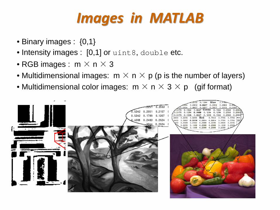
• Binary images : {0,1} • Intensity images : [0,1] or uint8, double etc. • RGB images : m × n × 3 • Multidimensional images: m × n × p (p is the number of layers) • Multidimensional color images: m × n × 3 × p (gif format)

Images in MATLAB

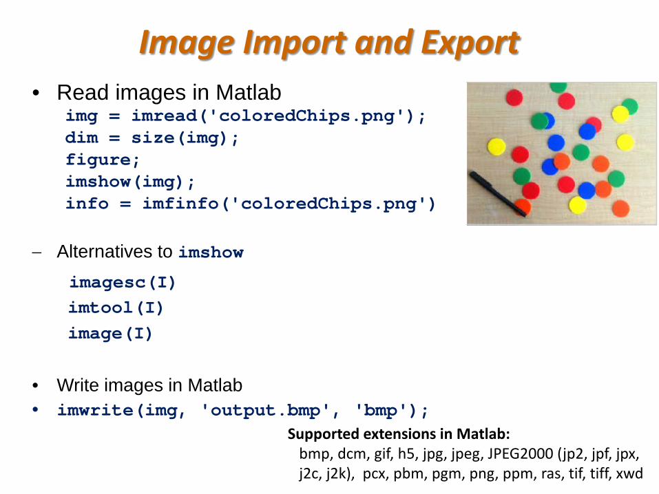
Image Import and Export • Read images in Matlab

img = imread('coloredChips.png'); dim = size(img); figure; imshow(img); info = imfinfo('coloredChips.png')

− Alternatives to imshow imagesc(I) imtool(I) image(I)

• Write images in Matlab • imwrite(img, 'output.bmp', 'bmp');

Supported extensions in Matlab: bmp, dcm, gif, h5, jpg, jpeg, JPEG2000 (jp2, jpf, jpx, j2c, j2k), pcx, pbm, pgm, png, ppm, ras, tif, tiff, xwd

Images

Images sind Matrizen!

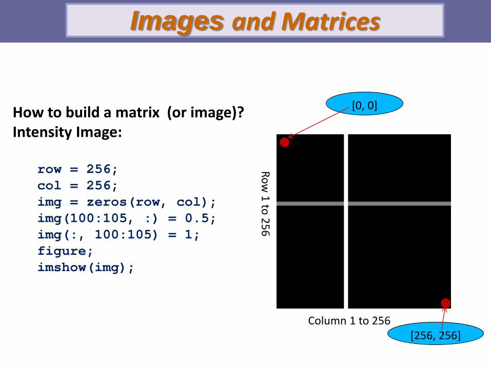
Column 1 to 256

Row 1 to 256

o

[0, 0]

o

[256, 256]

How to build a matrix (or image)? Intensity Image:

row = 256; col = 256; img = zeros(row, col); img(100:105, :) = 0.5; img(:, 100:105) = 1; figure; imshow(img);

Images and Matrices

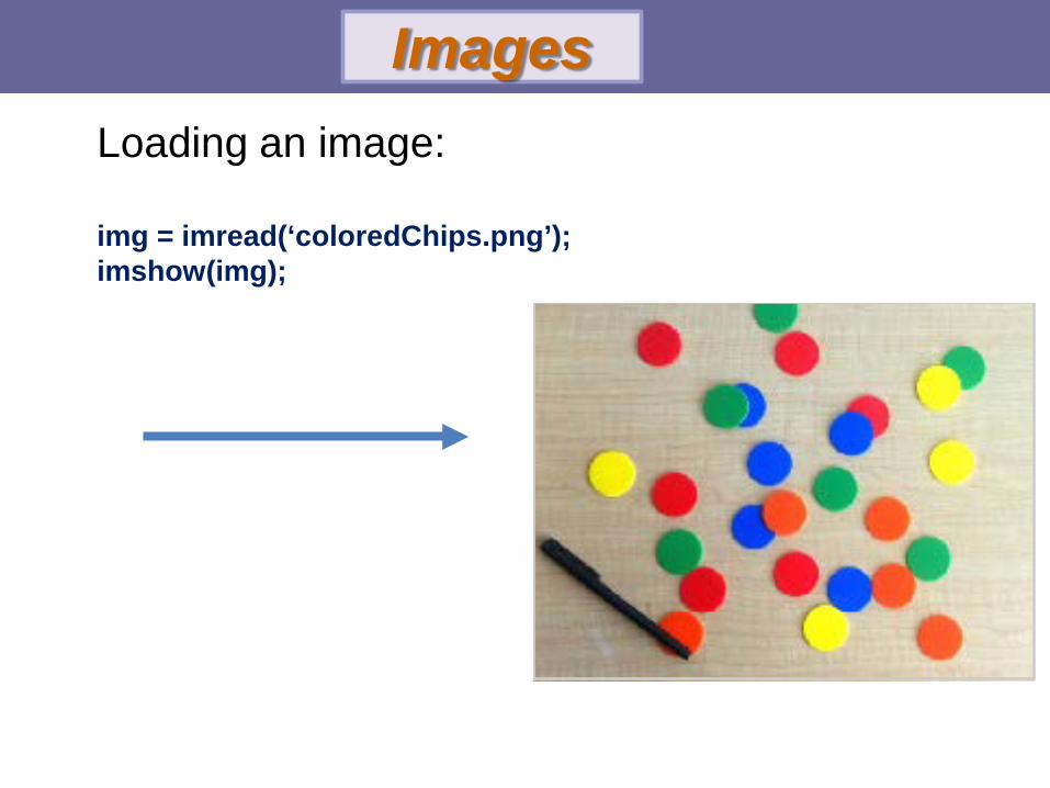
Loading an image: img = imread(‘coloredChips.png’); imshow(img);

Images

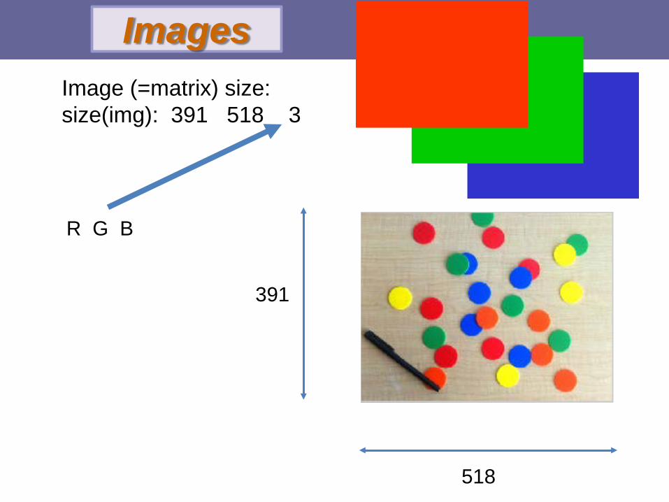
Image (=matrix) size: size(img): 391 518 3

R G B

391

518

Images

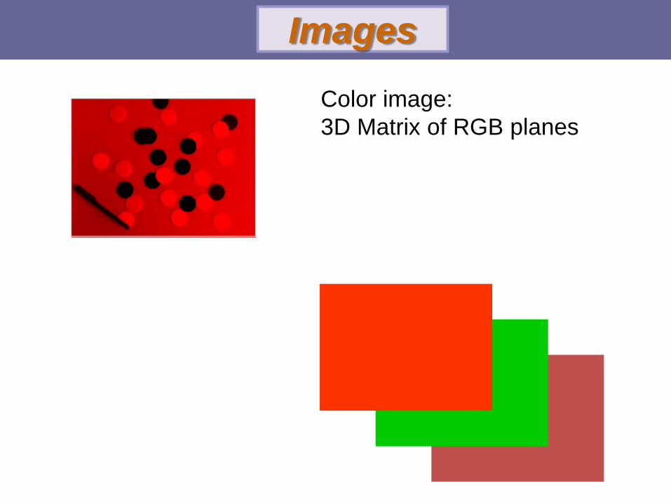
Color image: 3D Matrix of RGB planes

Images

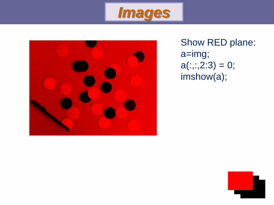
Show RED plane: a=img; a(:,:,2:3) = 0; imshow(a);

Images

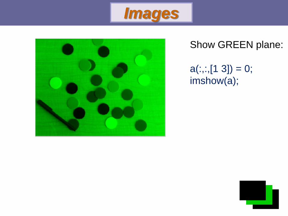
Show GREEN plane: a(:,:,[1 3]) = 0; imshow(a);

Images

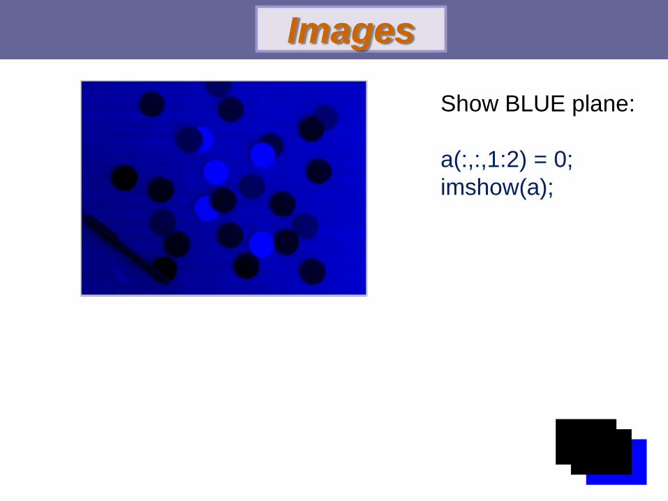
Show BLUE plane: a(:,:,1:2) = 0; imshow(a);

Images

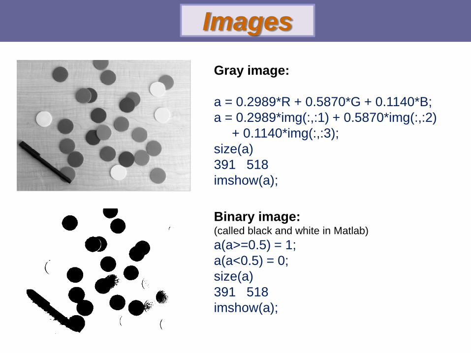
Gray image: a = 0.2989*R + 0.5870*G + 0.1140*B; a = 0.2989*img(:,:1) + 0.5870*img(:,:2) + 0.1140*img(:,:3); size(a) 391 518 imshow(a);

Images

Binary image: (called black and white in Matlab) a(a>=0.5) = 1; a(a<0.5) = 0; size(a) 391 518 imshow(a);

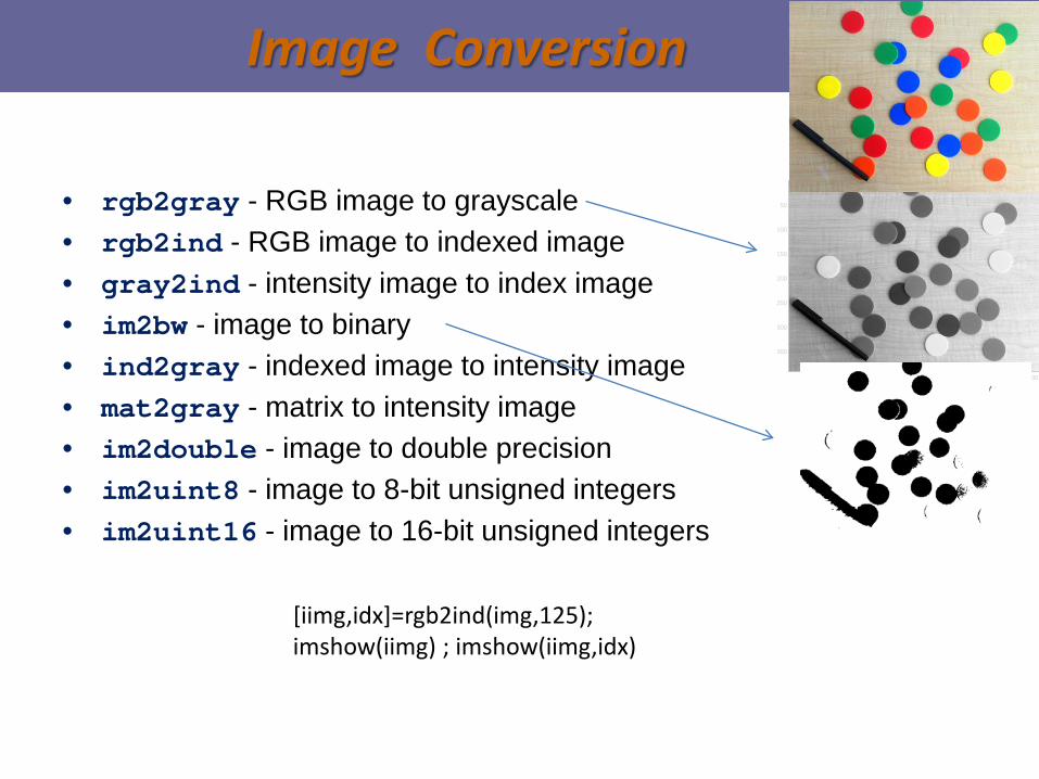
Image Conversion

• rgb2gray - RGB image to grayscale • rgb2ind - RGB image to indexed image • gray2ind - intensity image to index image • im2bw - image to binary • ind2gray - indexed image to intensity image • mat2gray - matrix to intensity image • im2double - image to double precision • im2uint8 - image to 8-bit unsigned integers • im2uint16 - image to 16-bit unsigned integers

50 100 150 200 250 300 350 400 450 500

50

100

150

200

250

300

350

[iimg,idx]=rgb2ind(img,125); imshow(iimg) ; imshow(iimg,idx)

Image Display

• Image - create and display image object • Imagesc - scale and display as image • imshow - display image • colorbar - display colorbar • colormap - sets the colormap to a m x 3 matrix where row is an RGB

vector that defines one color. (color coded data; Falschfarbendarstellung) >> im = imread(‘AT3_1m4_01.tif‘); imshow(im), colormap(jet); • truesize - adjust display size of image • zoom - zoom in and zoom out of 2D plot • getimage - get image data from axes

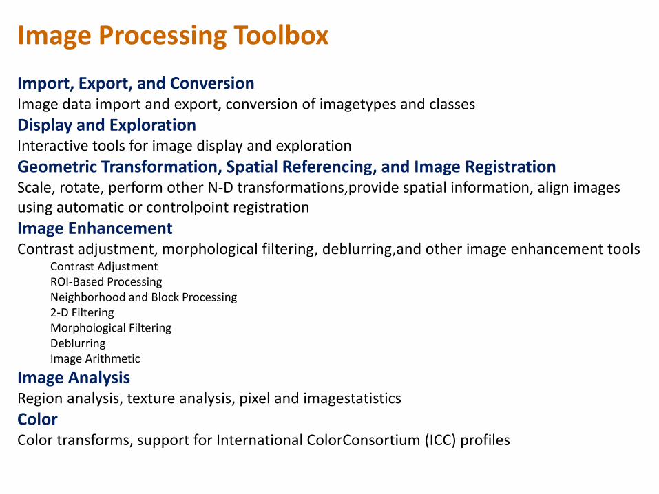
Image Processing Toolbox Import, Export, and Conversion Image data import and export, conversion of imagetypes and classes Display and Exploration Interactive tools for image display and exploration Geometric Transformation, Spatial Referencing, and Image Registration Scale, rotate, perform other N-D transformations,provide spatial information, align images using automatic or controlpoint registration Image Enhancement Contrast adjustment, morphological filtering, deblurring,and other image enhancement tools

Contrast Adjustment ROI-Based Processing Neighborhood and Block Processing 2-D Filtering Morphological Filtering Deblurring Image Arithmetic

Image Analysis Region analysis, texture analysis, pixel and imagestatistics Color Color transforms, support for International ColorConsortium (ICC) profiles

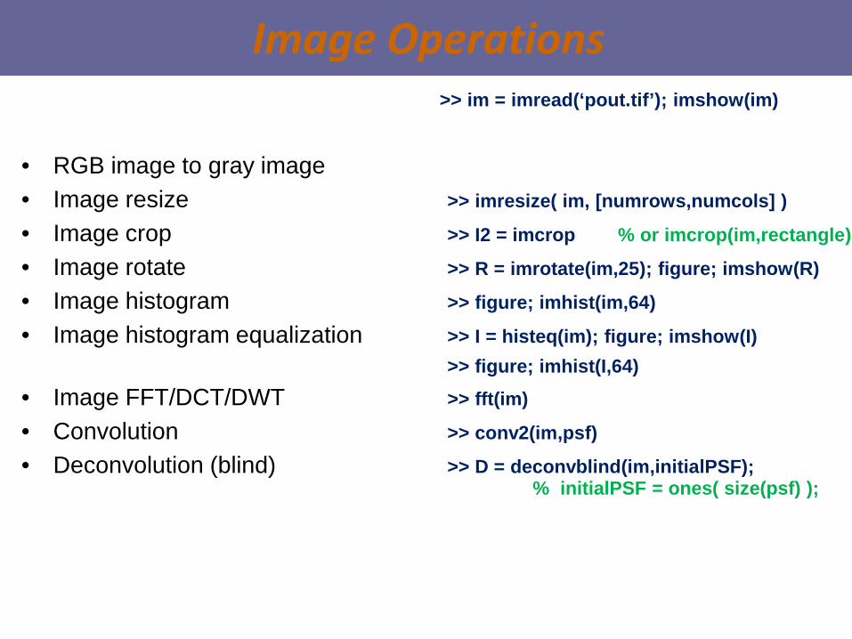
Image Operations

• RGB image to gray image • Image resize >> imresize( im, [numrows,numcols] )

• Image crop >> I2 = imcrop % or imcrop(im,rectangle)

• Image rotate >> R = imrotate(im,25); figure; imshow(R)

• Image histogram >> figure; imhist(im,64)

• Image histogram equalization >> I = histeq(im); figure; imshow(I) >> figure; imhist(I,64) • Image FFT/DCT/DWT >> fft(im)

• Convolution >> conv2(im,psf) • Deconvolution (blind) >> D = deconvblind(im,initialPSF);

% initialPSF = ones( size(psf) );

>> im = imread(‘pout.tif’); imshow(im)

Examples working with Images (1/3)

Create AVI movie with a series images

Video

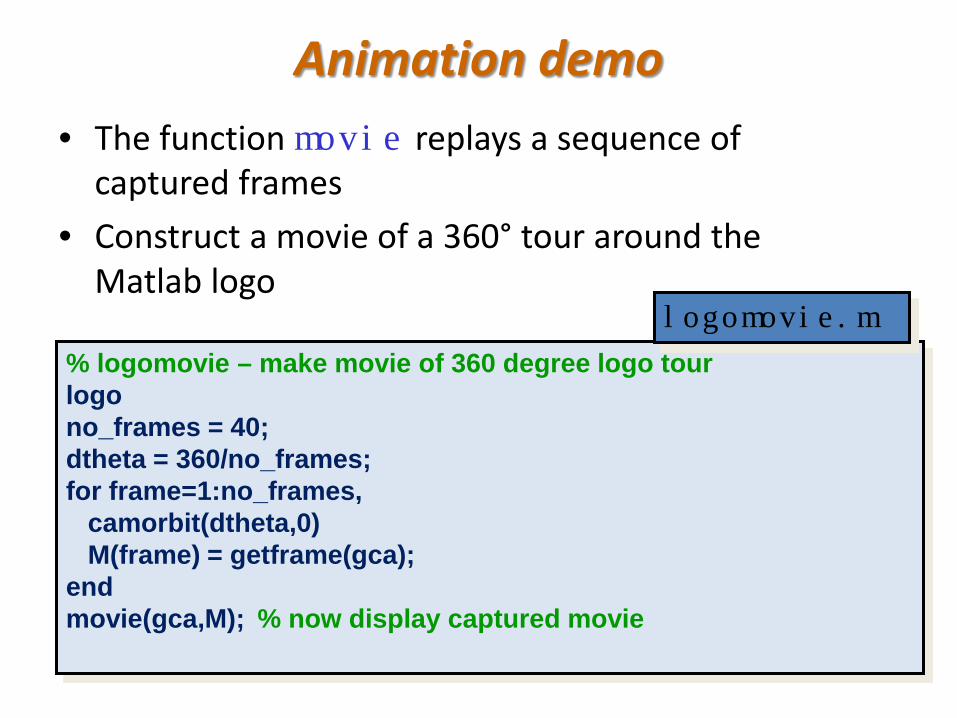
Animation demo • The function movie replays a sequence of

captured frames • Construct a movie of a 360° tour around the

Matlab logo

% logomovie – make movie of 360 degree logo tour logo no_frames = 40; dtheta = 360/no_frames; for frame=1:no_frames, camorbit(dtheta,0) M(frame) = getframe(gca); end movie(gca,M); % now display captured movie

logomovie.m

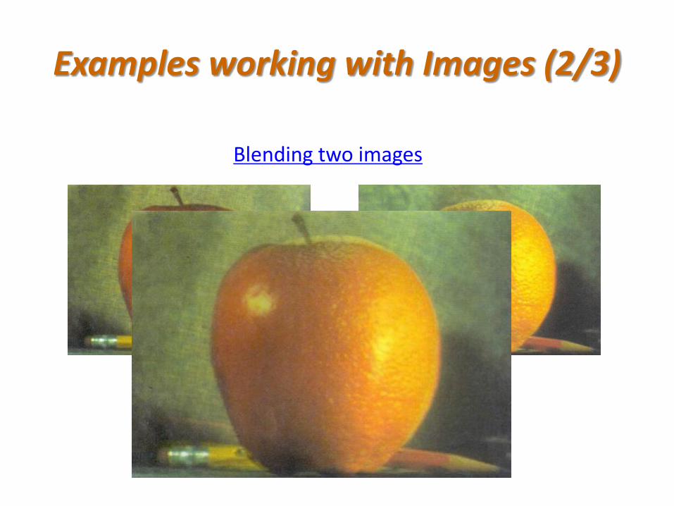
Blending two images

Examples working with Images (2/3)

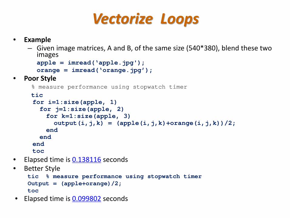
Vectorize Loops • Example

– Given image matrices, A and B, of the same size (540*380), blend these two images

apple = imread(‘apple.jpg'); orange = imread(‘orange.jpg’);

• Poor Style % measure performance using stopwatch timer tic for i=1:size(apple, 1) for j=1:size(apple, 2) for k=1:size(apple, 3) output(i,j,k) = (apple(i,j,k)+orange(i,j,k))/2; end end end toc • Elapsed time is 0.138116 seconds • Better Style

tic % measure performance using stopwatch timer Output = (apple+orange)/2; toc

• Elapsed time is 0.099802 seconds

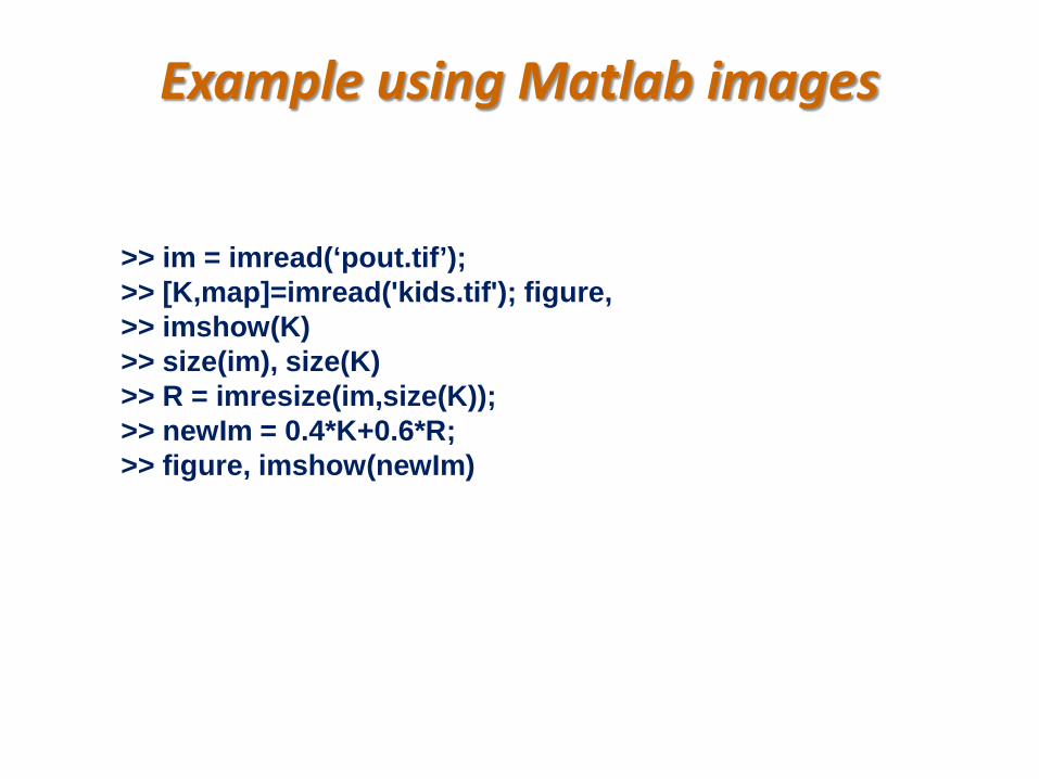
Example using Matlab images

>> im = imread(‘pout.tif’); >> [K,map]=imread('kids.tif'); figure, >> imshow(K) >> size(im), size(K) >> R = imresize(im,size(K)); >> newIm = 0.4*K+0.6*R; >> figure, imshow(newIm)

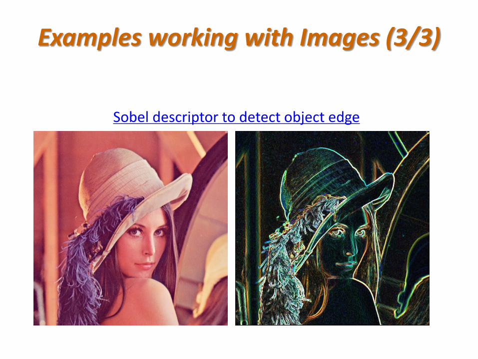
Sobel descriptor to detect object edge

Examples working with Images (3/3)

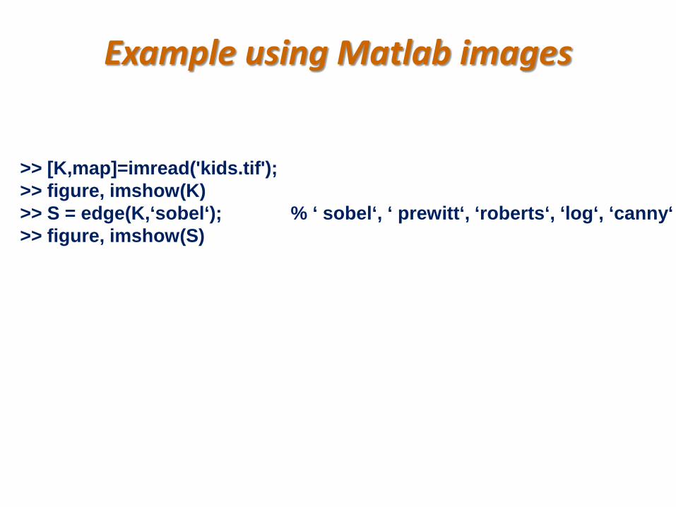
Example using Matlab images

>> [K,map]=imread('kids.tif'); >> figure, imshow(K) >> S = edge(K,‘sobel‘); % ‘ sobel‘, ‘ prewitt‘, ‘roberts‘, ‘log‘, ‘canny‘ >> figure, imshow(S)

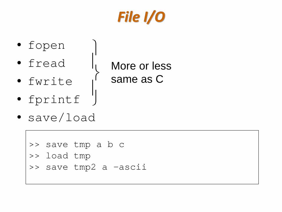
File I/O

• fopen

• fread

• fwrite

• fprintf

• save/load

More or less same as C

>> save tmp a b c >> load tmp >> save tmp2 a -ascii

• fileID = fopen(filename,perm) % Opens the file filename for binary reading; returns a positiv integer identifier (-1 if failed)

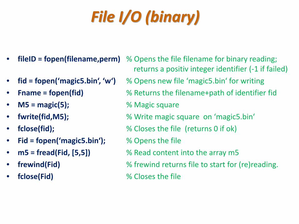
• fid = fopen(‘magic5.bin‘, ‘w‘) % Opens new file ‘magic5.bin‘ for writing • Fname = fopen(fid) % Returns the filename+path of identifier fid • M5 = magic(5); % Magic square • fwrite(fid,M5); % Write magic square on ‘magic5.bin‘ • fclose(fid); % Closes the file (returns 0 if ok) • Fid = fopen(‘magic5.bin‘); % Opens the file • m5 = fread(Fid, [5,5]) % Read content into the array m5 • frewind(Fid) % frewind returns file to start for (re)reading. • fclose(Fid) % Closes the file

File I/O (binary)

• fileID = fopen(filename,perm) % Opens the file filename for binary reading; returns a positiv integer identifier (-1 if failed)

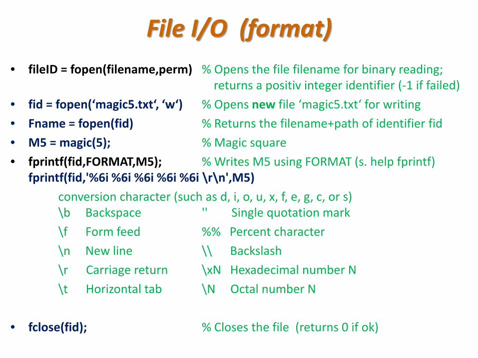
• fid = fopen(‘magic5.txt‘, ‘w‘) % Opens new file ‘magic5.txt‘ for writing • Fname = fopen(fid) % Returns the filename+path of identifier fid • M5 = magic(5); % Magic square • fprintf(fid,FORMAT,M5); % Writes M5 using FORMAT (s. help fprintf)

fprintf(fid,'%6i %6i %6i %6i %6i \r\n',M5) conversion character (such as d, i, o, u, x, f, e, g, c, or s) \b Backspace '' Single quotation mark \f Form feed %% Percent character \n New line \\ Backslash \r Carriage return \xN Hexadecimal number N \t Horizontal tab \N Octal number N • fclose(fid); % Closes the file (returns 0 if ok)

File I/O (format)

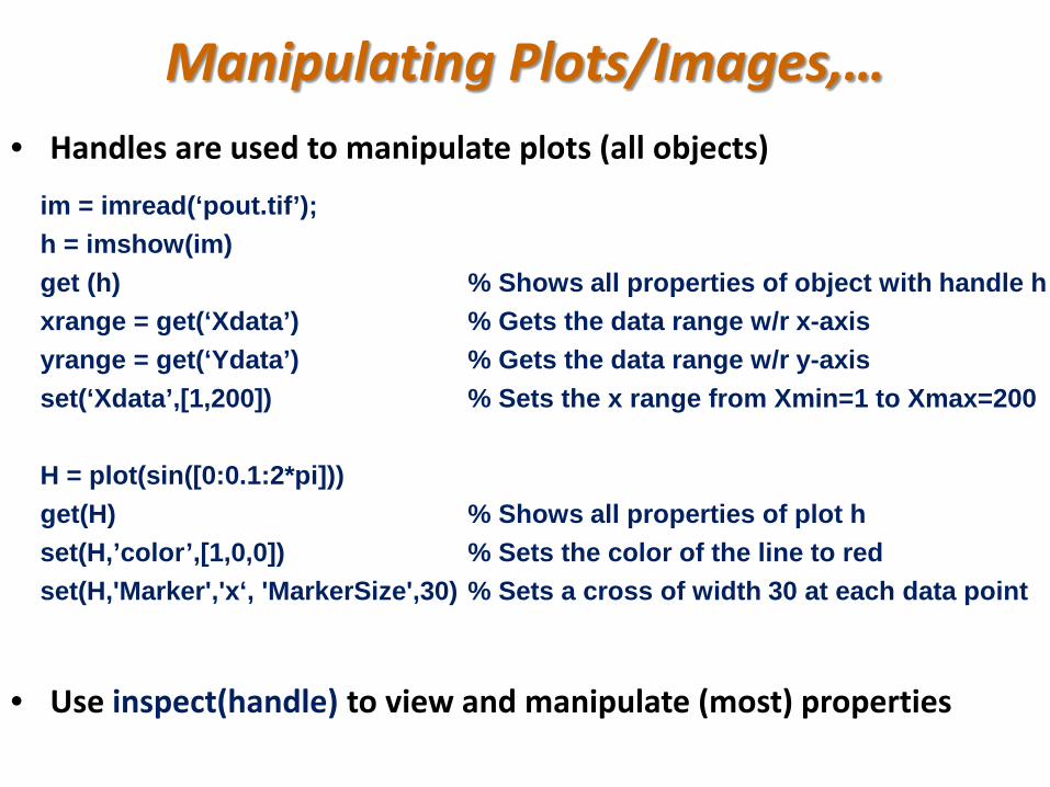
Manipulating Plots/Images,…

im = imread(‘pout.tif’); h = imshow(im) get (h) % Shows all properties of object with handle h xrange = get(‘Xdata’) % Gets the data range w/r x-axis yrange = get(‘Ydata’) % Gets the data range w/r y-axis set(‘Xdata’,[1,200]) % Sets the x range from Xmin=1 to Xmax=200 H = plot(sin([0:0.1:2*pi])) get(H) % Shows all properties of plot h set(H,’color’,[1,0,0]) % Sets the color of the line to red set(H,'Marker','x‘, 'MarkerSize',30) % Sets a cross of width 30 at each data point

• Handles are used to manipulate plots (all objects)

• Use inspect(handle) to view and manipulate (most) properties