MATLAB TUTORIAL

GETTING STARTED

WHAT IS MATLAB ?

MATLAB is a commercial "MATrix LABoratory" package, by MathWorks, which operates as aninteractive programming environment with graphical output. The MATLAB programminglanguage is exceptionally straightforward since almost every data object is assumed to be anarray. Hence, for some areas of engineering MATLAB is displacing popular programminglanguages, due to its interactive interface, reliable algorithmic foundation, fully extensibleenvironment, and computational speed. MATLAB is available for many different computersystems, including PCs and UNIX platforms.

THIS TUTORIAL

The purposes of this tutorial is to help you get started with MATLAB. We want you to see howMATLAB can be used in the solution of engineering problems.

Throughout this tutorial we assume that you:

1. Will read a couple of sections and then go to a computer to experiment with MATLAB.

2. Are familiar with UNIX or Windows 95.

3. Have access to supplementary material on matrices, matrix arithmetic/operations, andlinear algebra.

ENTERING AND RUNNING MATLAB

On a UNIX system, a MATLAB session may be entered by typing Unix Prompt> matlab <ENTER>

MATLAB will present the prompt

>>

On a system running Windows 95, double click on the MATLAB icon to launch and a commandwindow will appear with the prompt:

>>

You are now in MATLAB. From this point on, individual MATLAB commands may be given atthe program prompt. They will be processed when you hit the <ENTER> key. Many commandexamples are given below.

LEAVING MATLAB

A MATLAB session may be terminated by simply typing >> quit

or by typing >> exit

at the MATLAB prompt.

ONLINE HELP

Online help is available from the MATLAB prompt, both generally (listing all availablecommands). >> help [a long list of help topics follows]

and for specific commands:

>> help demo

A demonstration of various MATLAB functions can be explored with:

>> demo

A performance test of the machine running MATLAB can be done with:

>> bench

VARIABLES

MATLAB has built-in variables like pi, eps, and ans. You can learn their values from theMATLAB interpreter. >> eps eps =

2.2204e-16 >> pi ans =

3.1416

>> help pi

PI 3.1415926535897.... PI = 4*atan(1) = imag(log(-1)) = 3.1415926535897....

In MATLAB all numerical computing occurs with limited precision, with all decimal expansionsbeing truncated at the sixteenth place [roughly speaking]. The machine's round-off, the smallestdistinguishable difference between two numbers as represented in MATLAB, is denoted "eps".

The variable ans will keep track of the last output which was not assigned to another variable.

Variable Assignment : The equality sign is used to assign values to variables: >> x = 3

x =

3

>> y = x^2

y =

9

Variables in MATLAB are case sensitive. Hence, the variables "x" and "y" are distinct from "X"and "Y" (at this point, the latter are in fact, undefined).

Output can be suppressed by appending a semicolon to the command lines. >> x = 3; >> y = x^2; >> y

y =

9

As in C and Fortran, MATLAB variables must have a value [which might be numerical, or a stringof characters, for example]. Complex numbers are automatically available [by default, both i and jare initially aliased to sqrt(-1)].

Active Variables : At any time you want to know the active variables you can use who: >> who

Your variables are:

ans x y

Removing a Variable : To remove a variable, try this:

>> clear x

Saving and Restoring Variables : To save the value of the variable "x" to a plain text file named"x.value" use

>> save x.value x -ascii

To save all variables in a file named mysession.mat, in reloadable format, use

>> save mysession

To restore the session, use

>> load mysession

VARIABLE ARITHMETIC

MATLAB uses some fairly standard notation. More than one command may be entered on asingle line, if they are seperated by commas. >> 2+3; >> 3*4, 4^2;

Powers are performed before division and multiplication, which are done before subtraction andaddition. For example

>> 2+3*4^2;

generates ans = 50. That is:

2+3*4^2 ==> 2 + 3*4^2 <== exponent has the highest precedence ==> 2 + 3*16 <== then multiplication operator ==> 2 + 48 <== then addition operator ==> 50

Double Precision Arithmetic : All arithmetic is done to double precision, which for 32-bitmachines means to about 16 decimal digits of accuracy. Normally the results will be displayed in ashorter form.

>> a = sqrt(2)

a =

1.4142 >> format long, b=sqrt(2)

b =

1.41421356237310 >> format short

Command-Line Editing : The arrow keys allow "command-line editing," which cuts down onthe amount of typing required, and allows easy error correction. Press the "up" arrow, and add"/2." What will this produce?

>> 2+3*4^2/2

Parentheses may be used to group terms, or to make them more readable. For example:

>> (2 + 3*4^2)/2

generates ans = 25.

BUILT-IN MATHEMATICAL FUNCTIONS

MATLAB has a platter of built-in functions for mathematical and scientific computations. Here isa summary of relevant functions, followed by some examples: Function Meaning Example ==================================================== sin sine sin(pi) = 0.0 cos cosine cos(pi) = 1.0 tan tangent tan(pi/4) = 1.0 asin arcsine asin(pi/2)= 1.0 acos arccosine acos(pi/2)= 0.0 atan arctangent atan(pi/4)= 1.0 exp exponential exp(1.0) = 2.7183 log natural logarithm log(2.7183) = 1.0 log10 logarithm base 10 log10(100.0) = 2.0 ====================================================

The arguments to trigonometric functions are given in radians.

Example : Let's verify that sin(x)^2 + cos(x)^2 = 1.0

for arbitrary x. The MATLAB code is: >> format compact

>> x = pi/3; >> >> sin(x)^2 + cos(x)^2 - 1.0 ans = 0 >>

The "format compact" command eliminates spaces between the lines of output.

MATRICES

A matrix is a rectangular array of numbers. For example: [ 1 2 3 4 ] [ 4 5 6 7 ] [ 7 8 9 10 ]

defines a matrix with 3 rows, 4 columns, and 12 elements.

MATLAB works with essentially only one kind of object, a rectangular numerical matrixpossibly, with complex entries. Every MATLAB variable refers to a matrix [a number is a 1 by 1matrix]. In some situations, 1-by-1 matrices are interpreted as scalars, and matrices with only onerow or one column are interpreted as vectors.

ENGINEERING APPLICATION OF MATRICES

In the analysis of a wide range of engineering applications, matrices are a convenient means ofrepresenting transformations between coordinate systems, and for writing (moderate to large)families of equations representing the state of a system (e.g., equations of equilibrium, energy andmomentum conservation, and so forth).

Example : Suppose that the following three equations describe the equilibrium of a simplestructural system: 3 * x1 - 1 * x2 + 0 * x3 = 1 -1 * x1 + 4 * x2 - 2 * x3 = 5 0 * x1 - 2 * x2 + 10 * x3 = 26

This family of equations can be written in the form A.X = B, where

[ 3 -1 0 ] [ x1 ] [ 1 ] A = [ -1 6 -2 ], X = [ x2 ], and B = [ 5 ]. [ 0 -2 10 ] [ x3 ] [ 26 ]

In a typical application, matrices A and B will be defined by the parameters of the engineeringproblem, and the solution matrix X will need to be computed.

Depending on the specific values of coefficients in matrices A and B, there may be: (a) nosolutions to A.X = B, (b) a unique solution to A.X = B, or (c) an infinite number of solutions toA.X = B.

In this particular case, however, the solution matrix [ 1 ] X = [ 2 ] [ 3 ]

makes the right-hand side of the matrix equations (i.e., A.X) equal the left-hand side of the matrix

equations (i.e., matrix B). We will soon see how to setup and solve this family of matrix equationsin MATLAB (see examples below).

DEFINING MATRICES IN MATLAB

MATLAB is designed to make definition of matrices and matrix manipulation as simple aspossible.

Matrices can be introduced into MATLAB in several different ways:

Entered by an explicit list of elements,

C Generated by built-in statements and functions,

C Created in M-files (see below),

C Loaded from external data files (see details below).

For example, either of the statements >> A = [1 2 3; 4 5 6; 7 8 9];

and >> A = [ 1 2 3 4 5 6 7 8 9 ]

creates the obvious 3-by-3 matrix and assigns it to a variable A.

Note that:

The elements within a row of a matrix may be separated by commas as well as a blank.

C The elements of a matrix being entered are enclosed by brackets;

C A matrix is entered in "row-major order" [ie all of the first row, then all of the second row,etc];

C Rows are seperated by a semicolon [or a newline], and the elements of the row may beseperated by either a comma or a space. [Caution: Watch out for extra spaces!]

When listing a number in exponential form (e.g. 2.34e-9), blank spaces must be avoided. Listingentries of a large matrix is best done in an M-file (see section below), where errors can be easilyedited away.

The matrix element located in the i-th row and j-th column of a is referred to in the usual way: >> A(1,2), A(2,3) ans = 2 ans = 6 >>

It's very easy to modify matrices:

>> A(2,3) = 10;

Building Matrices from a Block : Large matrices can be assembled from smaller matrix blocks.For example, with matrix A in hand, we can enter the following commands;

>> C = [A; 10 11 12]; <== generates a (4x3) matrix >> [A; A; A]; <== generates a (9x3) matrix >> [A, A, A]; <== generates a (3x9) matrix

As with variables, use of a semicolon with matrices suppresses output. This feature can beespecially useful when large matrices are being generated.

If A is a 3-by-3 matrix, then >> B = [ A, zeros(3,2); zeros(2,3), eye(2) ];

will build a certain 5-by-5 matrix. Try it.

BUILT-IN MATRIX FUNCTIONS

MATLAB has many types of matrices which are built into the system e.g., Function Description =============================================== diag returns diagonal M.E. as vector eye identity matrix hilb Hilbert matrix magic magic square ones matrix of ones rand randomly generated matrix triu upper triangular part of a matrix tril lower triangular part of a matrix zeros matrix of zeros ===============================================

Here are some examples:

Matrices of Random Entries : A 3 by 3 matrix with random entries is produced by typing >> rand(3) ans = 0.0470 0.9347 0.8310 0.6789 0.3835 0.0346 0.6793 0.5194 0.0535 >>

General m-by-n matrices of random entries are generated with

>> rand(m,n);

Magic Squares : A magic square is a square matrix which has equal sums along all its rows andcolumns. For example:

>> magic(4) ans = 16 2 3 13 5 11 10 8 9 7 6 12 4 14 15 1 >>

The elements of each row and column sum to 34.

Matrices of Ones : The functions

eye (m,n) produces an m-by-n matrix of ones. eye (n) produces an n-by-n matrix of ones.

Matrices of Zeros : The commands

zeros (m,n) produces an m-by-n matrix of zeros. zeros (n) produces an n-by-n one;

If A is a matrix, then zeros(A) produces a matrix of zeros of the same size as A.

Diagonal Matrices : If x is a vector, diag(x) is the diagonal matrix with x down the diagonal.

if A is a square matrix, then diag(A) is a vector consisting of the diagonal of A.

What is diag(diag(A))? Try it.

MATRIX OPERATIONS

The following matrix operations are available in MATLAB: Operator Description Operator Description ============================================================ + addition ' transpose - subtraction \ left division * multiplication / right division ^ power ============================================================

These matrix operations apply, of course, to scalars (1-by-1 matrices) as well. If the sizes of thematrices are incompatible for the matrix operation, an error message will result, except in the caseof scalar-matrix operations (for addition, subtraction, and division as well as for multiplication) inwhich case each entry of the matrix is operated on by the scalar.

Matrix Transpose : The transpose of a matrix is the result of interchanging rows and columns.MATLAB denotes the [conjugate] transpose by following the matrix with the single-quote[apostrophe]. For example: >> A' ans =

1 4 7 2 5 8 3 6 9 >> B = [1+i 2 + 2*i 3 - 3*i]' B =

1.0000 - 1.0000i 2.0000 - 2.0000i 3.0000 + 3.0000i >>

Matrix Addition/Subtraction : Let matrix "A" have m rows and n columns, and matrix "B" havep rows and q columns. The matrix sum "A + B" is defined only when m equals p and n = q, Theresult is a n-by-m matrix having the element-by-element sum of components in A and B.

For example: >> E = [ 2 3; 4 5.0; 6 7]; >> F = [ 1 -2; 3 6.5; 10 -45];

>> E+F ans = 3.0000 1.0000 7.0000 11.5000 16.0000 -38.0000 >>

Matrix Multiplication : Matrix multiplication requires that the sizes match. If they don't, anerror message is generated.

>> A*B, B*A; >> B'*A; >> A*A', A'*A; >> B'*B, B*B';

Scalars multiply matrices as expected, and matrices may be added in the usual way (both are done"element by element@):

>> 2*A, A/4; >> A + [b,b,b];

Example: We can use matrix multiplication to check the "magic" property of magic squares.

>> A = magic(5); >> b = ones(5,1); >> A*b; <== (5x1) matrix containing row sums. >> v = ones(1,5); >> v*A; <== (1x5) matrix containing column sums.

Matrix Functions "any" and "all" : There is a function to determine if a matrix has at least onenonzero entry, any, as well as a function to determine if all the entries are nonzero, all.

>> A = zeros(1,4) >> any(A) >> D = ones(1,4) >> any(D) >> all(A)

Returning more than One Value : Some MATLAB functions can return more than one value.In the case of max the interpreter returns the maximum value and also the column index where themaximum value occurs.

>> [m, i] = max(B) >> min(A) >> b = 2*ones(A) >> A*B >> A

Round Floating Point numbers to Integers : MATLAB has functions to round floating pointnumbers to integers. MATLAB has functions to round floating point numbers to integers. Theseare round, fix, ceil, and floor. The next few examples work through this set of commands anda couple more arithmetic operations.

>> f = [-.5 .1 .5]; >> round(f) >> fix(f) >> ceil(f) >> floor(f) >> sum(f) >> prod(f)

MATRIX-ELEMENT LEVEL OPERATIONS

The matrix operations of addition and subtraction already operate on an element-by-element basis,but the other matrix operations given above do not -- they are matrix operations.

MATLAB has a convention in which a dot in front of the operations, * , ^ , \ , and /,

will force them to perform entry-by-entry operation instead of the usual matrix operation. Forexample [1,2,3,4].*[1,2,3,4]

ans =

1 4 9 16

The same result can be obtained with

[1,2,3,4].^2

Element-by-element operations are particularly useful for MATLAB graphics.

SYSTEMS OF LINEAR EQUATIONS

One of the main uses of matrices is in representing systems of linear equations. Let: "A" A matrix containing the coefficients of a system of linear equations, "X" A column vector containing the "unknowns." "B" A column vector of "right-hand side constant terms".

The linear system of equations is represented by the matrix equation

A X = B

In MATLAB, solutions to the matrix equations are computed with Amatrix division@ operations.More precisely:

>> X=A\B

is the solution of A*X=B (this can be read "matrix X equals the inverse of matrix A, multiplied byB) and,

>> X=B/A

is the solution of x*A=b . For the case of left division, if A is square, then it is factored usingGaussian elimination and these factors are used to solve A*x=b.

Comment for Numerical Gurus : If A is not square, then it is factored using Householderorthogonalization with column pivoting and the factors are used to solve the under- or over-determined system in the least squares sense. Right division is defined in terms of left division by >> b/A=(A' \ b')'

NUMERICAL EXAMPLE

In the opening sections of this tutorial we discussed the family of equations given by: >> A = [ 3 -1 0; -1 6 -2; 0 -2 10 ]; >> B = [ 1; 5; 26 ];

The solution to these equations is given by:

>> X = A \ B X = 1.0000 2.0000 3.0000 >>

and X agrees with our initial observation. We can check the solution by verify that

A*X ==> B and A*X - B ==> 0

The required MATLAB commands are:

>> A*X ans = 1.0000 5.0000 26.0000 >> A*X - B ans = 1.0e-14 * 0.0444 -0.2665 -0.3553 >>

Note : If there is no solution, a "least-squares" solution is provided (i.e., A*X - B is as small aspossible).

CONTROL STRUCTURES

Control-of-flow in MATLAB programs is achieved with logical/relational constructs, branchingconstructs, and a variety of looping constructs.

Colon Notation : A central part of the MATLAB language syntax is the "colon operator," whichproduces a list. For example: >> format compact >> -3:3 ans = -3 -2 -1 0 1 2 3

The default increment is by 1, but that can be changed. For example:

>> x = -3 : .3 : 3 x = Columns 1 through 7 -3.0000 -2.7000 -2.4000 -2.1000 -1.8000 -1.5000 -1.2000 Columns 8 through 14 -0.9000 -0.6000 -0.3000 0 0.3000 0.6000 0.9000 Columns 15 through 21 1.2000 1.5000 1.8000 2.1000 2.4000 2.7000 3.0000 >>

This can be read: "x is the name of the list, which begins at -3, and whose entries increase by .3,until 3 is surpassed." You may think of x as a list, a vector, or a matrix, whichever you like.

In our third example, the following statements generate a table of sines. >> x = [0.0:0.1:2.0]' ; >> y = sin(x); >> [x y]

Try it. Note that since sin operates entry-wise, it produces a vector y from the vector x.

The colon notation can also be combined with the earlier method of constructing matrices. >> a = [1:6 ; 2:7 ; 4:9]

RELATIONAL AND LOGICAL CONSTRUCTS

The relational operators in MATLAB are Operator Description =================================== < less than > greater than <= less than or equal >= greater than or equal == equal ~= not equal. ===================================

Note that ``='' is used in an assignment statement while ``=='' is used in a relation.

Relations may be connected or quantified by the logical operators Operator Description =================================== & and | or ~ not. ===================================

When applied to scalars, a relation is actually the scalar 1 or 0 depending on whether the relationis true or false (indeed, throughout this section you should think of 1 as true and 0 as false). Forexample

>> 3 < 5 ans = 1 >> a = 3 == 5 a = 0 >>

When logical operands are applied to matrices of the same size, a relation is a matrix of 0's and 1'sgiving the value of the relation between corresponding entries. For example:

>> A = [ 1 2; 3 4 ]; >> B = [ 6 7; 8 9 ]; >> A == B ans = 0 0 0 0 >> A < B ans =

1 1 1 1

>>

To see how the other logical operators work, you should also try

>> ~A >> A&B >> A & ~B >> A | B >> A | ~A

The for statement permits any matrix to be used instead of 1:n.

BRANCHING CONSTRUCTS

MATLAB provides a number of language constructs for branching a program's control of flow.

if-end Construct : The most basic construct is: if <condition>, <program> end

Here the condition is a logical expression that will evaluate to either true or false (i.e., with values1 or 0). When the logical expression evaluates to 0, the program control moves on to the nextprogram construction. You should keep in mind that MATLAB regards A==B and A<=B asfunctions with values 0 or 1.

Example : >> a = 1; >> b = 2; >> if a < b, c = 3; end; >> c

c =

3

>>

If-else-end Construct : Frequently, this construction is elaborated with

if <condition1>, <program1> else <program2> end

In this case if condition is 0, then program2 is executed.

If-elseif-end Construct : Another variation is if <condition1>, <program1> elseif <condition2>, <program2> end

Now if condition1 is not 0, then program1 is executed, if condition1 is 0 and if condition2 is not

0, then program2 is executed, and otherwise control is passed on to the next construction.

LOOPING CONSTRUCTS

For Loops : A for loop is a construction of the form for i= 1 : n, <program>, end

The program will repeat <program> once for each index value i = 1, 2 .... n. Here are someexamples of MATLAB's for loop capabilities:

Example : The basic for loop >> for i = 1 : 5, c = 2*i end c = 2

..... lines of output removed ...

c = 10 >>

computes and prints "c = 2*i" for i = 1, 2, ... 5.

Example : For looping constructs may be nested.

Here is an example of creating a matrices contents inside a nested for loop: >> for i=1:10, for j=1:10, A(i,j) = i/j; end end >> A

There are actually two loops here, with one nested inside the other; they define

A(1,1), A(1,2), A(1,3) ... A(1,10), A(2,1), ... A(10,10)

in that order.

Example : MATLAB will allow you to put any vector in place of the vector 1:n in thisconstruction. Thus the construction >> for i = [2,4,5,6,10], <program>, end

is perfectly legitimate.

In this case program will execute 5 times and the values for the variable i during execution aresuccessively, 2,4,5,6,10.

Example : The MATLAB developers went one step further. If you can put a vector in, why notput a matrix in? So, for example, >> for i=magic(7),

<program>, end

is also legal. Now the program will execute 7 (=number of columns) times, and the values of iused in program will be successively the columns of magic(7).

While Loops : A while loop is a construction of the form while <condition>, <program>, end

where condition is a MATLAB function, as with the branching construction. The programprogram will execute successively as long as the value of condition is not 0. While loops carry animplicit danger in that there is no guarantee in general that you will exit a while loop. Here is asample program using a while loop.

function l=twolog(n)

% l=twolog(n). l is the floor of the base 2 % logarithm of n.

l=0; m=2; while m<=n l=l+1; m=2*m; end

SOME NOTES

A relation between matrices is interpreted by while and if to be true if each entry of the relationmatrix is nonzero. Hence, if you wish to execute statement when matrices A and B are equal youcould type if A == B statement end

but if you wish to execute statement when A and B are not equal, you would type

if any(any(A ~ B)) ( statement ) end

or, more simply,

if A == B else { statement } end

SUB-MATRICES

We have already seen how colon notation can be used to generate vectors. A very common use ofthe colon notation is to extract rows, or columns, as a sort of "wild-card" operator whichproduces a default list. For example, A(1:4,3)

is the column vector consisting of the first four entries of the third column of A . A colon by itself

denotes an entire row or column. So, for example: A(:,3)

is the third column of A , and A(1:4,:)

is the first four rows of A. Arbitrary integral vectors can be used as subscripts. The statement A(:,[2 4])

contains as columns, columns 2 and 4 of matrix A. This subscripting scheme can be used on bothsides of an assignment statement: A(:,[2 4 5]) = B(:,1:3)

replaces columns 2,4,5 of matrix A with the first three columns of matrix B. Note that the "entire"altered matrix A is printed and assigned. Try it.

Columns 2 and 4 of A can be multiplied on the right by the 2-by-2 matrix [1 2;3 4]: A(:,[2,4]) = A(:,[2,4])*[1 2;3 4]

Once again, the entire altered matrix is printed and assigned.

When you a insert a 0-1 vector into the column position then the columns which correspond to 1'sare displayed. >> V=[0 1 0 1 1] >> A(:,V) >> A(V,:)

MATLAB SCRIPTING FILES

PROGRAM DEVELOPMENT WITH M-FILES

MATLAB statements can be prepared with any editor, and stored in a file for later use. Such a fileis referred to as a script, or an "M-file" (since they must have a name extension of the formfilename.m). Writing M-files will enhance your problem solving productivity since manyMATLAB commands can be run from one file without having to enter each command one-by-oneat the MATLAB prompt. This way, corrections and changes can be made in the M-file and re-runeasily.

Suppose that we create a program file myfile.m

in the MATLAB language. The commands in this file can be exectued by simply giving thecommand >> myfile

from MATLAB. The MATLAB statements will run like any other MATLAB function. You donot need to compile the program since MATLAB is an interpretative (not compiled) language.

An M-file can reference other M-files, including referencing itself recursively.

Example : Using your favorite editor, create the following file, named sketch.m: [x y] = meshgrid(-3:.1:3, -3:.1:3);

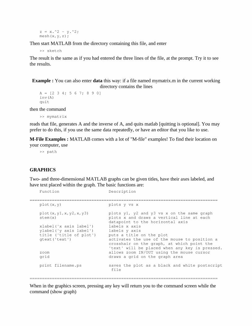
z = x.^2 - y.^2; mesh(x,y,z);

Then start MATLAB from the directory containing this file, and enter

>> sketch

The result is the same as if you had entered the three lines of the file, at the prompt. Try it to seethe results.

Example : You can also enter data this way: if a file named mymatrix.m in the current workingdirectory contains the lines

A = [2 3 4; 5 6 7; 8 9 0] inv(A) quit

then the command

>> mymatrix

reads that file, generates A and the inverse of A, and quits matlab [quitting is optional]. You mayprefer to do this, if you use the same data repeatedly, or have an editor that you like to use.

M-File Examples : MATLAB comes with a lot of "M-file" examples! To find their location onyour computer, use >> path

GRAPHICS

Two- and three-dimensional MATLAB graphs can be given titles, have their axes labeled, andhave text placed within the graph. The basic functions are: Function Description ============================================================================ plot(x,y) plots y vs x

plot(x,y1,x,y2,x,y3) plots y1, y2 and y3 vs x on the same graph stem(x) plots x and draws a vertical line at each

datapoint to the horizontal axis xlabel('x axis label') labels x axis ylabel('y axis label') labels y axis title ('title of plot') puts a title on the plot gtext('text') activates the use of the mouse to position a crosshair on the graph, at which point the 'text' will be placed when any key is pressed. zoom allows zoom IN/OUT using the mouse cursor grid draws a grid on the graph area

print filename.ps saves the plot as a black and white postscript file

============================================================================

When in the graphics screen, pressing any key will return you to the command screen while thecommand (show graph)

>> shg

will return you to the current graphics screen. If your machine supports multiple windows with aseparate graphics window, you will want to keep the graphics window exposed-but moved to theside-and the command window active.

MATLAB graphics windows will contain one plot by default. The command subplot can be usedto partition the screen so that up to four plots can be viewed simultaneously. For moreinformation, type >> help subplot

TWO-DIMENSIONAL PLOTS

The plot command creates linear x-y plots; if x and y are vectors of the same length, thecommand plot(x,y) opens a graphics window and draws an x-y plot of the elements of x versusthe elements of y.

Example : Let's draw the graph of the sine function over the interval -4 to 4 with the followingcommands: >> x = -4:.01:4; y = sin(x); plot(x,y) >> grid >> xlabel('x') >> ylabel('sin(x)')

The vector x is a partition of the domain with meshsize 0.01 while y is a vector giving the valuesof sine at the nodes of this partition (recall that sin operates entrywise). Try it to see the results.

Example : Plots of parametrically defined curves can also be made. For example, >> t=0:.001:2*pi; x=cos(3*t); y=sin(2*t); plot(x,y)

Example : Two ways to make multiple plots on a single graph are illustrated by >> x = 0:.01:2*pi;y1=sin(x);y2=sin(2*x); >> y3 = sin(4*x);plot(x,y1,x,y2,x,y3)

and by forming a matrix Y containing the functional values as columns

>> x=0:.01:2*pi; Y=[sin(x)', sin(2*x)', sin(4*x)']; plot(x,Y)

Another way is with hold. The command hold freezes the current graphics screen so thatsubsequent plots are superimposed on it. Entering hold again releases the ``hold.''

Example : One can override the default linetypes and pointtypes. For example, the commandsequence >> x = 0:.01:2*pi; y1=sin(x); y2=sin(2*x); y3=sin(4*x); >> plot(x,y1,'--',x,y2,':',x,y3,'+') >> grid >> title ('Dashed line and dotted line graph')

renders a dashed line and dotted line for the first two graphs while for the third the symbol isplaced at each node. Try it.

The line-type and mark-type are ============================================================= Linetypes : solid (-), dashed (-). dotted (:), dashdot (-.) Marktypes : point (.), plus (+), star (*, circle (o),

x-mark (x) =============================================================

See help plot for line and mark colors.

THREE-DIMENSIONAL GRAPHICS

Three dimensional mesh surface plots are drawn with the functions Function Description ============================================================================= mesh(z) Creates a three-dimensional perspective plot of the elementsof the matrix "z". The mesh surface is defined by the z-coordinates of points above a rectangular grid in the x-y plane. =============================================================================

To draw the graph of a function

z = f(x,y)

over a rectangle, one first defines vectors xx and yy, which give partitions of the sides of therectangle.

With the function meshdom (mesh domain; called meshgrid in version 4.0) one then creates amatrix x, each row of which equals xx and whose column length is the length of yy, and similarlya matrix y, each column of which equals yy, as follows: >> [x,y] = meshdom(xx,yy);

One then computes a matrix z, obtained by evaluating f entrywise over the matrices x and y, towhich mesh can be applied.

Example : Suppose that we want to draw a graph of over the square [-2,2] x [-2,2] asfollows: >> xx = -2:.1:2; >> yy = xx; >> [x,y] = meshdom(xx,yy); >> z = exp(-x.^2 - y.^2); >> mesh(z)

Of course one could replace the first three lines of the preceding with >> [x,y] = meshdom(-2:.1:2, -2:.1:2);

See the User's Guide for further details regarding mesh. Also see information on functions plot3,and surf.

CREATING POSTCRIPT HARDCOPIES

To create a black-and-white postcript file of a MATLAB figure just type >> print name-of-figure.ps

Color postscript files can be generated with >> print -dpsc name-of-figure.ps

Similarly, try the command

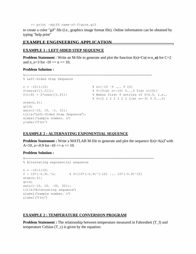
>> print -dgif8 name-of-figure.gif

to create a color "gif" file (i.e., graphics image format file). Online information can be obtained bytyping "help print"

EXAMPLE ENGINEERING APPLICATION

EXAMPLE 1 : LEFT-SIDED STEP SEQUENCE

Problem Statement : Write an M-file to generate and plot the function f(n)=Cu(-n-n_o) for C=2and n_o=3 for -10 <= n <= 10.

Problem Solution :%==================================================================% Left-Sided Step Sequence

n = -10:1:10; % n=[-10 -9 ... 9 10]f=zeros([1,21]); % f=[0(at n=-10) 0...0 0(at n=10)]f(1:8) = 2*ones([1,8]); % Makes first 8 entries of f=2.0, i.e.,

% f=[2 2 2 2 2 2 2 2(at n=-3) 0 0...0]stem(n,f);grid;axis([-10, 10, -1, 3]);title(>Left-Sided Step Sequence=);xlabel(>sample number, n=)ylabel(>f(n)=)

EXAMPLE 2 : ALTERNATING EXPONENTIAL SEQUENCE

Problem Statement : Write a MATLAB M-file to generate and plot the sequence f(n)=A(a)n withA=10, a=-0.9 for -10 <= n <= 10.

Problem Solution :%===================================================================% Alternating exponential sequence

n = -10:1:10;f = 10*(-0.9).^n; % f=[10*(-0.9)^(-10) ... 10*(-0.9)^10]stem(n,f);grid;axis([-10, 10, -30, 30]);title(>Alternating sequence=)xlabel(>sample number, n=)ylabel(>f(n)=)

EXAMPLE 2 : TEMPERATURE CONVERSION PROGRAM

Problem Statement : The relationship between temperature measured in Fahrenheit (T_f) andtemperature Celsius (T_c) is given by the equation:

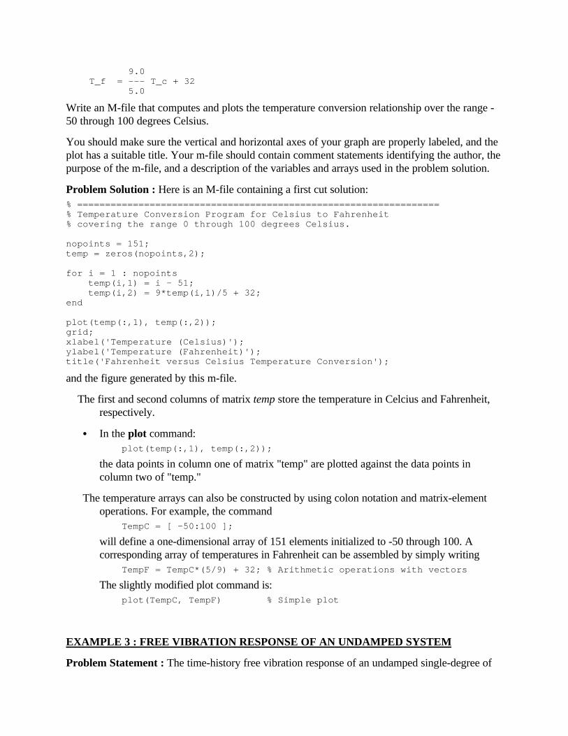
9.0 T_f = --- T_c + 32 5.0

Write an M-file that computes and plots the temperature conversion relationship over the range -50 through 100 degrees Celsius.

You should make sure the vertical and horizontal axes of your graph are properly labeled, and theplot has a suitable title. Your m-file should contain comment statements identifying the author, thepurpose of the m-file, and a description of the variables and arrays used in the problem solution.

Problem Solution : Here is an M-file containing a first cut solution:% =================================================================% Temperature Conversion Program for Celsius to Fahrenheit% covering the range 0 through 100 degrees Celsius.

nopoints = 151;temp = zeros(nopoints,2);

for i = 1 : nopoints temp(i,1) = i - 51; temp(i,2) = 9*temp(i,1)/5 + 32;end

plot(temp(:,1), temp(:,2));grid;xlabel('Temperature (Celsius)');ylabel('Temperature (Fahrenheit)');title('Fahrenheit versus Celsius Temperature Conversion');

and the figure generated by this m-file.

The first and second columns of matrix temp store the temperature in Celcius and Fahrenheit,respectively.

C In the plot command: plot(temp(:,1), temp(:,2));

the data points in column one of matrix "temp" are plotted against the data points incolumn two of "temp."

The temperature arrays can also be constructed by using colon notation and matrix-elementoperations. For example, the command TempC = [ -50:100 ];

will define a one-dimensional array of 151 elements initialized to -50 through 100. Acorresponding array of temperatures in Fahrenheit can be assembled by simply writing TempF = TempC*(5/9) + 32; % Arithmetic operations with vectors

The slightly modified plot command is: plot(TempC, TempF) % Simple plot

EXAMPLE 3 : FREE VIBRATION RESPONSE OF AN UNDAMPED SYSTEM

Problem Statement : The time-history free vibration response of an undamped single-degree of

freedom oscillator is given by: v(o) x(t) = x(0) cos (wt) + ---- sin (wt) w

where,

t = time. x(t) = displacement at time t. v(t) = velocity at time t. w = sqrt(k/m) = circular natural frequency of the system. m = the system mass. k = the system stiffness.

The natural period of this system is

T = 2*pi*sqrt(m/k).

Now let's suppose that the system has mass = 1, stiffness = 10, and an initial displacement andvelocity x(0) = 10 and v(0) = 10.

Write a MATLAB M-file that will compute and plot the "displacement versus time" (i.e., x(t)versus t) and "velocity versus time" (i.e., v(t) versus t ) for the time interval 0 through 10 seconds.To ensure that your plot will be reasonably smooth, choose an increment in your displacement andvelocity calculations that is no larger than 1/10 of the system period T. (An elegant solution to thisproblem would do this automatically).

Solution : Here is an M-file containing a first cut solution:% =================================================================% Compute dynamic response of an undamped system.

% Setup array for storing and plotting system response

nopoints = 501;response = zeros(nopoints,3);

% Problem parameters and initial conditions

mass = 1;stiff = 10;w = sqrt(stiff/mass);dt = 0.02;

displ0 = 1;velocity0 = 10;

% Compute displacement and velocity time history response

for i = 1 : nopoints + 1 time = (i-1)*dt; response(i,1) = time; response(i,2) = displ0*cos(w*time) + velocity0/w*sin(w*time); response(i,3) = -displ0*w*sin(w*time) + velocity0*cos(w*time);end

% Plot displacement versus time

plot(response(:,1), response(:,2));hold;

% Plot velocity versus time

plot(response(:,1), response(:,3));grid;xlabel('Time (seconds)');ylabel('Displacement (m) and Velocity (m/sec)');title('Time-History Response for SDOF Oscillator');

The velocity of the system versus time is given by the derivative of the displacement withrespect to time. In mathematical terms: d v(t) = -- x(t) = -displ0*w*sin(w*t) + velocity0*cos(w*t); dt

where displ0 and velocity0 are the displacement and velocity of the system at t = 0.

The natural period of this system is T = 2*pi*sqrt(m/k) = 6.282/sqrt(10) = 2.0 seconds.

The timestep increment dt = 0.02 seconds easily satisfies the stated criteria for a smoothgraph.

The first column of response stores the time, and the second and third columns of response thedisplacement and velocity, respectively.

C A second way of computing the time, displacement, and velocity vectors is time = 0.0:0.02:10; displ = displ0*cos(w*time) + velocity0/w*sin(w*time); velocity = -displ0*w*sin(w*time) + velocity0*cos(w*time);

The first statement generates a (1x501) matrix called time having the element values 0,0.02, 0.04 .... 10.0. The dimensions of matrices "displ" and "velocity" are inferred from thedimensions of "temp" with the values of the matrix elements given by the evaluation offormulae on the right-hand side of the assignment statements.

Now the plots can be generated with: plot(time, displ); hold; plot(time, velocity);

So how do we know that these graphs might be correct? First, notice that at t = 0 seconds, thedisplacement and velocity graphs both match the stated initial conditions. Second, notethat because the initial velocity is greater than zero, we expect the displacement curve toinitially increase. It does. A final point to note is the relationship between the displacementand velocity. When the oscillator displacemnt is at either its maximum or minimum value,the mass will be at rest for a short time. In mathematical terms, peak values in thedisplacement curve correspond to zero values in the velocity curve.

MISCELLANEOUS FEATURES

You may have discovered by now that MATLAB is case sensitive, that is "a" is not the same as "A."

If this proves to be an annoyance, the command >> casesen

will toggle the case sensitivity off and on.

The MATLAB display only shows 5 digits in the default mode. The fact is that MATLAB alwayskeeps and computes in a double precision 16 decimal places and rounds the display to 4 digits.The command >> format long

will switch to display all 16 digits and >> format short

will return to the shorter display. It is also possible to toggle back and forth in the scientificnotation display with the commands >> format short e

and >> format long e

It is not always necessary for MATLAB to display the results of a command to the screen. If youdo not want the matrix A displayed, put a semicolon after it, A;. When MATLAB is ready toproceed, the prompt >> will appear. Try this on a matrix right now.

Sometimes you will have spent much time creating matrices in the course of your MATLABsession and you would like to use these same matrices in your next session. You can save thesevalues in a file by typing >> save filename

This creates a file filename.mat

which contains the values of the variables from your session. If you do not want to save allvariables there are two options. One is to clear the variables off with the command >> clear a b c

which will remove the variables a,b,c. The other option is to use the command >> save x y z

which will save the variables x,y,z in the file filename.mat. The variables can be reloaded in afuture session by typing >> load filename

When you are ready to print out the results of a session, you can store the results in a file and printthe file from the operating system using the "print" command appropriate for your operatingsystem. The file is created using the command

>> diary filename

Once a file name has been established you can toggle the diary with the commands >> diary on

and >> diary off

This will copy anything which goes to the screen (other than graphics) to the specified file. Sincethis is an ordinary ASCII file, you can edit it later.

I am going to describe the basic programming constructions. While there are other constructionsavailable, if you master these you will be able to write clear programs.

PROGRAMMING SUGGESTIONS

Here are a few pointers for programming in MATLAB:

1. use indented style that you have seen in the above programs. It makes the programs easierto read, the program syntax is easier to check, and it forces you to think in terms ofbuilding your programs in blocks.

2. Put lots of comments in your program to tell the reader in plain English what is going on.Some day that reader will be you, and you will wonder what you did.

3. Put error messages in your programs like the ones above. As you go through this manual,your programs will build on each other. Error messages will help you debug futureprograms.

4. Always structure your output as if it will be the input of another function. For example, ifyour program has "yes-no" type output, do not have it return the words "yes" and "no,"rather return 1 or 0, so that it can be used as a condition for a branch or while loopconstruction in the future.

5. In MATLAB, try to avoid loops in your programs. MATLAB is optimized to run the built-in functions. For a comparison, see how much faster A*B is over mult(A,B). You will beamazed at how much economy can be achieved with MATLAB functions.

6. If you are having trouble writing a program, get a small part of it running and try to buildon that. With reference to 5), write the program first with loops, if necessary, then go backand improve it.

ACKNOWLEDGEMENTS

This tutorial is a modified version of Mark Austin=s Matlab Tutorial, University of Maryland,College Park.