MATRICES - Muarchive.mu.ac.in/myweb_test/syllFybscit/APM.pdf · 1 1 MATRICES UNIT STRUCTURE 1.0 Objectives 1.1 Introduction 1.2 Definitions 1.3 Illustrative examples 1.4 Rank of matrix

1

1 MATRICES

UNIT STRUCTURE

1.0 Objectives

1.1 Introduction

1.2 Definitions

1.3 Illustrative examples

1.4 Rank of matrix

1.5 Canonical form or Normal form

1.6 Normal form PAQ

1.7 Let Us Sum Up

1.8 Unit End Exercise

1.0 OBJECTIVES

In this chapter a student has to learn the

Concept of adjoint of a matrix.

Inverse of a matrix.

Rank of a matrix and methods finding these.

1.1 INTRODUCTION

At higher secondary level, we have studied the definition of a matrix,

operations on the matrices, types of matrices inverse of a matrix etc.

In this chapter, we are studying adjoint method of finding the inverse of a

square matrix and also the rank of a matrix.

1.2 DEFINITIONS

1) Definitions:- A system of m n numbers arranged in the form of

an ordered set of m horizontal lines called rows & n vertical lines called

columns is called an m n matrix.

The matrix of order m n is written as

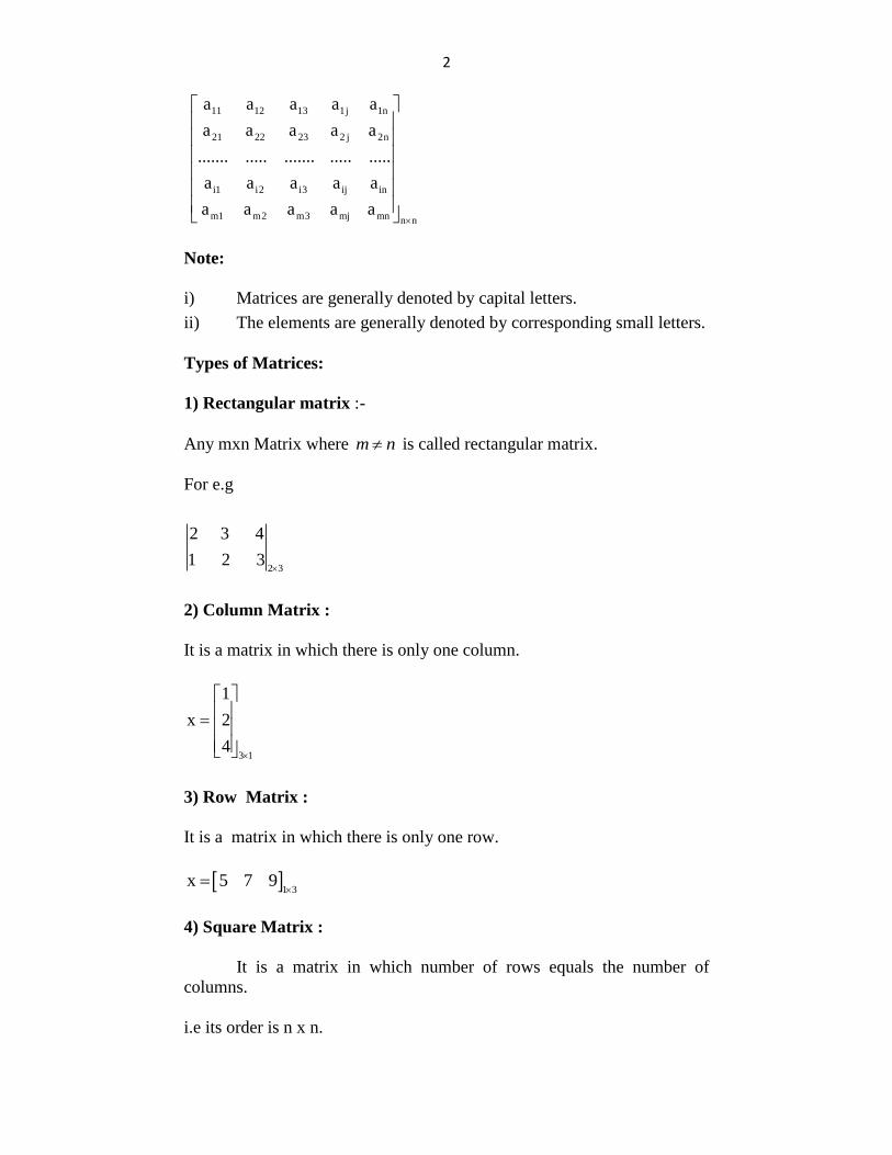
2

11 12 13 1j 1n

21 22 23 2 j 2n

i1 i2 i3 ij in

m1 m2 m3 mj mn n n

a a a a a

a a a a a

....... ..... ....... ..... .....

a a a a a

a a a a a

Note:

i) Matrices are generally denoted by capital letters.

ii) The elements are generally denoted by corresponding small letters.

Types of Matrices:

1) Rectangular matrix :-

Any mxn Matrix where m n is called rectangular matrix.

For e.g

2 3

2 3 4

1 2 3

2) Column Matrix :

It is a matrix in which there is only one column.

3 1

1

x 2

4

3) Row Matrix :

It is a matrix in which there is only one row.

1 3

x 5 7 9

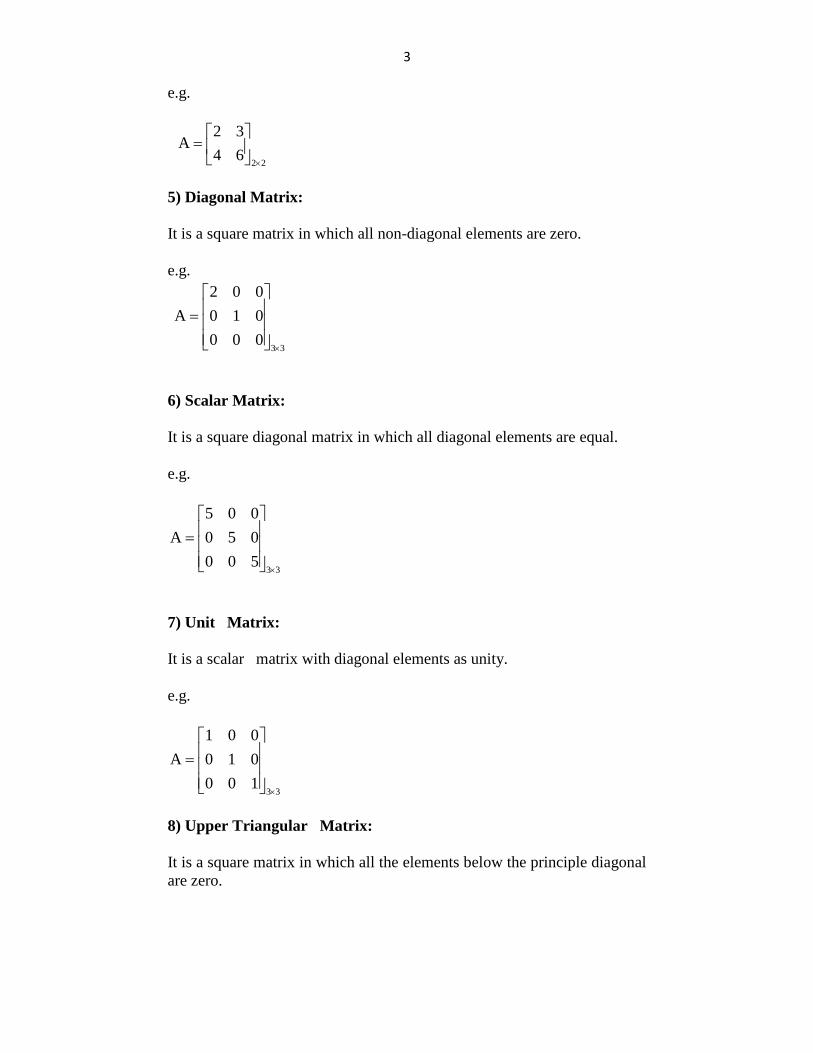
4) Square Matrix :

It is a matrix in which number of rows equals the number of

columns.

i.e its order is n x n.

3

e.g.

2 2

2 3 A

4 6

5) Diagonal Matrix:

It is a square matrix in which all non-diagonal elements are zero.

e.g.

3 3

2 0 0

A 0 1 0

0 0 0

6) Scalar Matrix:

It is a square diagonal matrix in which all diagonal elements are equal.

e.g.

3 3

5 0 0

A 0 5 0

0 0 5

7) Unit Matrix:

It is a scalar matrix with diagonal elements as unity.

e.g.

3 3

1 0 0

A 0 1 0

0 0 1

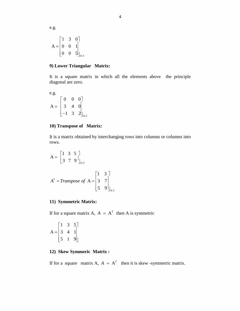
8) Upper Triangular Matrix:

It is a square matrix in which all the elements below the principle diagonal

are zero.

4

e.g.

3 3

1 3 0

A 0 0 1

0 0 5

9) Lower Triangular Matrix:

It is a square matrix in which all the elements above the principle

diagonal are zero.

e.g.

3 3

0 0 0

A 3 4 0

1 3 2

10) Transpose of Matrix:

It is a matrix obtained by interchanging rows into columns or columns into

rows.

2 3

1 3 5 A

3 7 9

3 2

1 3

A 3 7

5 9

TA Transpose of

11) Symmetric Matrix:

If for a square matrix A,

A TA then A is symmetric

1 3 5

A 3 4 1

5 1 9

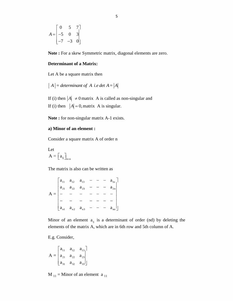
12) Skew Symmeric Matrix :

If for a square matrix A,

A TA then it is skew -symmetric matrix.

5

0 5 7

5 0 3

7 3 0

A

Note : For a skew Symmetric matrix, diagonal elements are zero.

Determinant of a Matrix:

Let A be a square matrix then

A = determinant of A i.e det A= A

If (i) then 0A matrix A is called as non-singular and

If (i) then 0,A matrix A is singular.

Note : for non-singular matrix A-1 exists.

a) Minor of an element :

Consider a square matrix A of order n

Let

ij n nA = a

The matrix is also can be written as

11 12 13 1n

21 22 23 2n

n1 n2 n3 nn

a a a a

a a a a

A =

a a a a

Minor of an element ija is a determinant of order (nd) by deleting the

elements of the matrix A, which are in 6th row and 5th column of A.

E.g. Consider,

11 12 13

21 22 23

31 32 33

a a a

A = a a a

a a a

M 11 = Minor of an element a 11

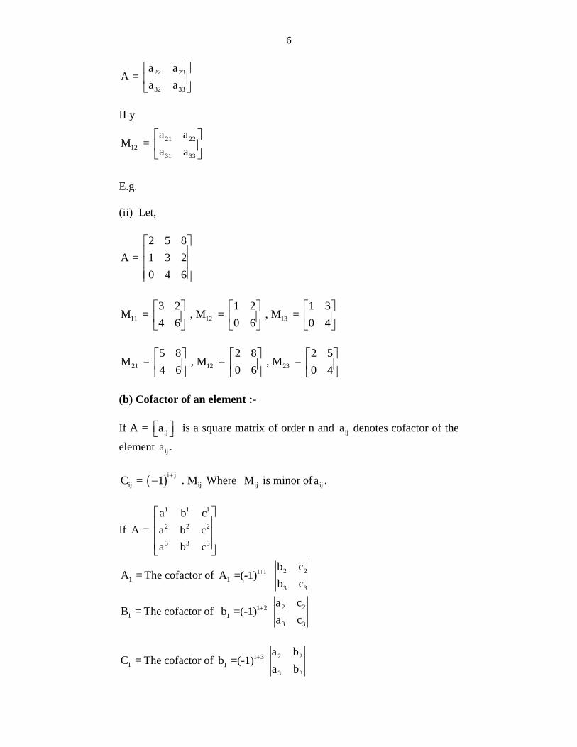
6

22 23

32 33

a aA =

a a

II y

21 22

12

31 33

a aM =

a a

E.g.

(ii) Let,

2 5 8

A = 1 3 2

0 4 6

11 12 13

3 2 1 2 1 3M = , M = , M =

4 6 0 6 0 4

21 12 23

5 8 2 8 2 5M = , M = , M =

4 6 0 6 0 4

(b) Cofactor of an element :-

If A = ija is a square matrix of order n and ija denotes cofactor of the

element ija .

i j

ij ijC = 1 . M

Where ij M is minor of ija .

If

1 1 1

2 2 2

3 3 3

a b c

A = a b c

a b c

1A = The cofactor of 1 1

1A =(-1) 2 2

3 3

b c

b c

1B = The cofactor of 1 2

1b =(-1) 2 2

3 3

a c

a c

1C = The cofactor of 1 3

1b =(-1) 2 2

3 3

a b

a b

7

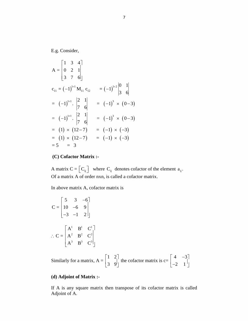
E.g. Consider,

1 3 4

A = 0 2 1

3 7 6

1 1 1 2

11 11 12

0 1c = 1 M c = 1

3 6

1 1 32 1

= 1 . = 1 0 37 6

1 1 32 1

= 1 . = 1 0 37 6

= 1 12 7 = 1 3

= 1 12 7 = 1 3

= 5 = 3

(C) Cofactor Matrix :-

A matrix C = ijC where ijC denotes cofactor of the element ija .

Of a matrix A of order nxn, is called a cofactor matrix.

In above matrix A, cofactor matrix is

5 3 6

C = 10 6 9

3 1 2

1 1 1

2 2 2

3 3 3

A B C

C = A B C

A B C

Similarly for a matrix, A = 1 2

3 9

the cofactor matrix is c= 4 3

2 1

(d) Adjoint of Matrix :-

If A is any square matrix then transpose of its cofactor matrix is called

Adjoint of A.

8

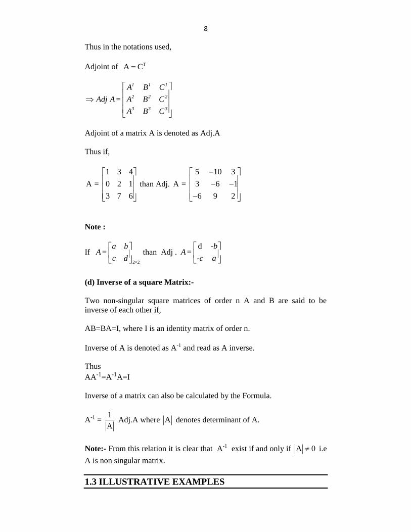
Thus in the notations used,

Adjoint of TA C

1 1 1

2 2 2

3 3 3

A B C

Adj A = A B C

A B C

Adjoint of a matrix A is denoted as Adj.A

Thus if,

1 3 4

A = 0 2 1

3 7 6

than Adj.

5 10 3

A = 3 6 1

6 9 2

Note :

If 2×2

a bA =

c d

than Adj . d -b

A = -c a

(d) Inverse of a square Matrix:-

Two non-singular square matrices of order n A and B are said to be

inverse of each other if,

AB=BA=I, where I is an identity matrix of order n.

Inverse of A is denoted as A-1 and read as A inverse.

Thus

AA-1=A-1A=I

Inverse of a matrix can also be calculated by the Formula.

A-1 = 1

A Adj.A where A denotes determinant of A.

Note:- From this relation it is clear that A-1 exist if and only if A 0 i.e

A is non singular matrix.

1.3 ILLUSTRATIVE EXAMPLES

9

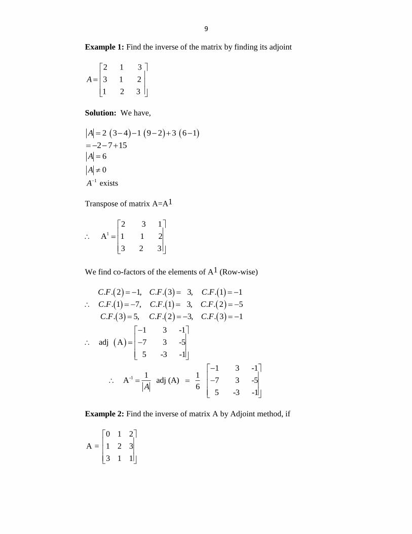
Example 1: Find the inverse of the matrix by finding its adjoint

2 1 3

3 1 2

1 2 3

A

Solution: We have,

2 3 4 1 9 2 3 6 1A

2 7 15

6A

0A

1A exists

Transpose of matrix A=A1

1

2 3 1

A 1 1 2

3 2 3

We find co-factors of the elements of A1 (Row-wise)

. . 2 1, . . 3 3, . . 1 1

. . 1 7, . . 1 3, . . 2 5

. . 3 5, . . 2 3, . . 3 1

C F C F C F

C F C F C F

C F C F C F

1 3 -1

adj A 7 3 -5

5 -3 -1

-1

1 3 -11 1

A adj (A) 7 3 -56

5 -3 -1A

Example 2: Find the inverse of matrix A by Adjoint method, if

0 1 2

A = 1 2 3

3 1 1

10

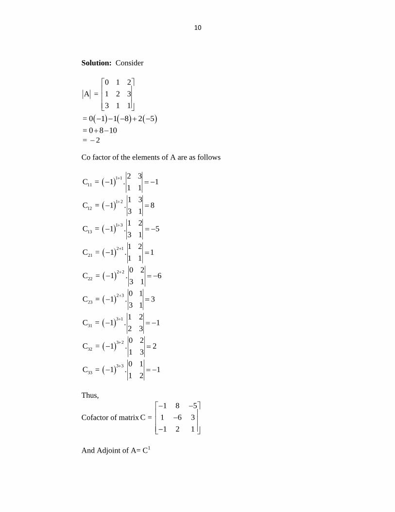
Solution: Consider

0 1 2

A = 1 2 3

3 1 1

= 0 1 1 8 2 5

= 0 8 10

= 2

Co factor of the elements of A are as follows

1 1

11

2 3C = 1 . 1

1 1

1 2

12

1 3C = 1 . 8

3 1

1 3

13

1 2C = 1 . 5

3 1

2 1

21

1 2C = 1 . 1

1 1

2 2

22

0 2C = 1 . 6

3 1

2 3

23

0 1C = 1 . 3

3 1

3 1

31

1 2C = 1 . 1

2 3

3 2

32

0 2C = 1 . 2

1 3

3 3

33

0 1C = 1 . 1

1 2

Thus,

Cofactor of matrix

1 8 5

C = 1 6 3

1 2 1

And Adjoint of A= C1

11

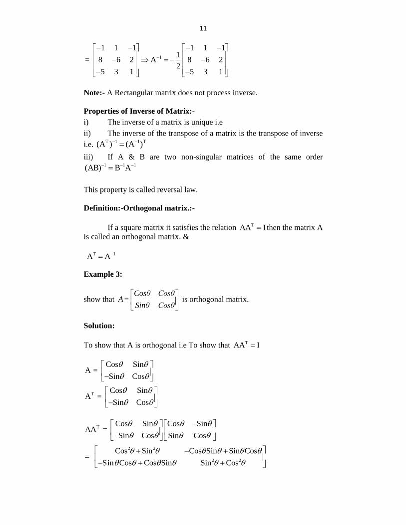
1

1 1 1 1 1 11

= 8 6 2 A 8 6 22

5 3 1 5 3 1

Note:- A Rectangular matrix does not process inverse.

Properties of Inverse of Matrix:-

i) The inverse of a matrix is unique i.e

ii) The inverse of the transpose of a matrix is the transpose of inverse

i.e. T 1 1 T(A ) (A )

iii) If A & B are two non-singular matrices of the same order

1 1 1(AB) B A

This property is called reversal law.

Definition:-Orthogonal matrix.:-

If a square matrix it satisfies the relation TAA I then the matrix A

is called an orthogonal matrix. &

T 1A A

Example 3:

show thatCosθ Cosθ

A = Sinθ Cosθ

is orthogonal matrix.

Solution:

To show that A is orthogonal i.e To show that TAA I

Cos SinA =

Sin Cos

TCos Sin

A = Sin Cos

TCos Sin Cos Sin

AA = Sin Cos Sin Cos

2 2

2 2

Cos Sin Cos Sin Sin Cos

Sin Cos Cos Sin Sin Cos

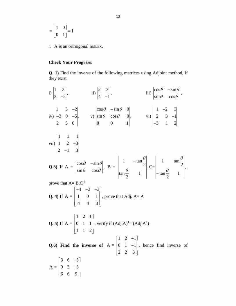
12

1 0= I

0 1

A is an orthogonal matrix.

Check Your Progress:

Q. 1) Find the inverse of the following matrices using Adjoint method, if

they exist.

i) 1 2

,2 2

ii) 2 3

,4 1

iii) cos sin

,sin cos

iv)

1 3 2

3 0 5 ,

2 5 0

v)

cos sin 0

sin cos 0 ,

0 0 1

vi)

1 2 3

2 3 1

3 1 2

vii)

1 1 1

1 2 3

2 1 3

Q.3) If A = cos sin

,sin cos

B =

1 tan2

,

tan 12

C=

1 tan2

,

tan 12

,

prove that A= B.C-1

Q. 4) If

4 3 3

A = 1 0 1

4 4 3

, prove that Adj. A= A

Q. 5) If

1 2 1

A = 0 1 1

1 1 2

, verify if (Adj.A)1= (Adj.A1)

Q.6) Find the inverse of

1 2 1

A = 0 1 1

2 2 3

, hence find inverse of

3 6 3

A = 0 3 3

6 6 9

13

1.4 RANK OF A MATRIX

a) Minor of a matrix

Let A be any given matrix of order mxn. The determinant of any

submatrix of a square order is called minor of the matrix A.

We observe that, if „r‟ denotes the order of a minor of a matrix of

order mxn then 1 r m if m<n and 1 r n if n<m.

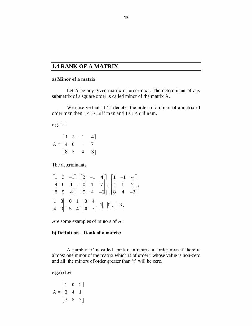
e.g. Let

1 3 1 4

A = 4 0 1 7

8 5 4 3

The determinants

1 3 1 3 1 4 1 1 4

4 0 1 , 0 1 7 , 4 1 7 ,

8 5 4 5 4 3 8 4 3

1 3 0 1 3 4, , , 1 , 0 , 3 ,

4 0 5 4 0 7

Are some examples of minors of A.

b) Definition – Rank of a matrix:

A number „r‟ is called rank of a matrix of order mxn if there is

almost one minor of the matrix which is of order r whose value is non-zero

and all the minors of order greater than „r‟ will be zero.

e.g.(i) Let

1 0 2

A = 2 4 1

3 5 7

14

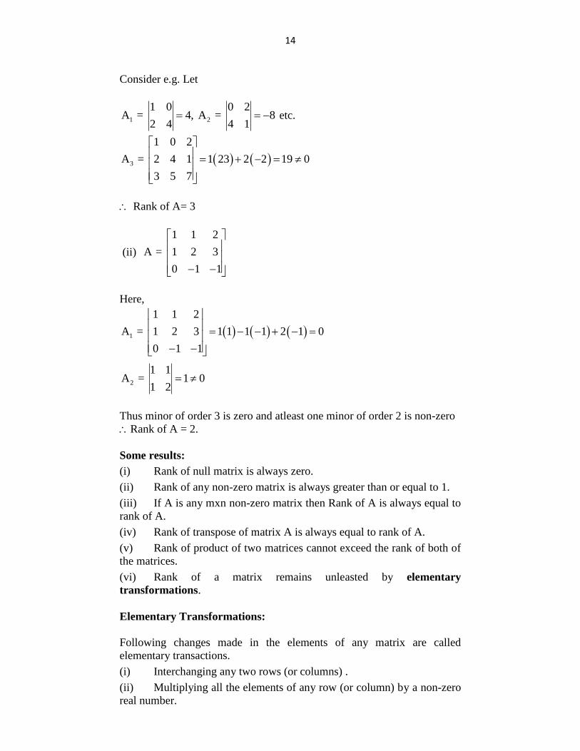
Consider e.g. Let

1 2

1 0 0 2A = 4, A = 8

2 4 4 1

etc.

3

1 0 2

A = 2 4 1 1 23 2 2 19 0

3 5 7

Rank of A= 3

(ii)

1 1 2

A = 1 2 3

0 1 1

Here,

1

1 1 2

A = 1 2 3 1 1 1 1 2 1 0

0 1 1

2

1 1A = 1 0

1 2

Thus minor of order 3 is zero and atleast one minor of order 2 is non-zero

Rank of A = 2.

Some results:

(i) Rank of null matrix is always zero.

(ii) Rank of any non-zero matrix is always greater than or equal to 1.

(iii) If A is any mxn non-zero matrix then Rank of A is always equal to

rank of A.

(iv) Rank of transpose of matrix A is always equal to rank of A.

(v) Rank of product of two matrices cannot exceed the rank of both of

the matrices.

(vi) Rank of a matrix remains unleasted by elementary

transformations.

Elementary Transformations:

Following changes made in the elements of any matrix are called

elementary transactions.

(i) Interchanging any two rows (or columns) .

(ii) Multiplying all the elements of any row (or column) by a non-zero

real number.

15

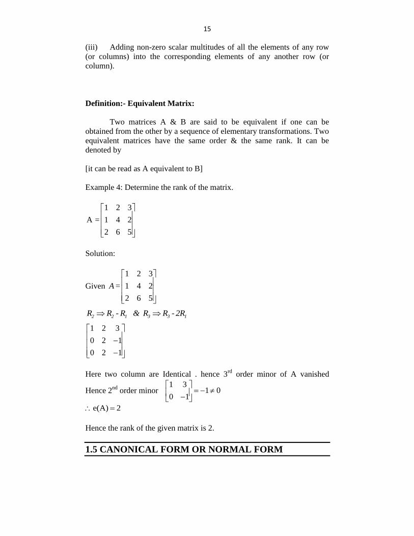
(iii) Adding non-zero scalar multitudes of all the elements of any row

(or columns) into the corresponding elements of any another row (or

column).

Definition:- Equivalent Matrix:

Two matrices A & B are said to be equivalent if one can be

obtained from the other by a sequence of elementary transformations. Two

equivalent matrices have the same order & the same rank. It can be

denoted by

[it can be read as A equivalent to B]

Example 4: Determine the rank of the matrix.

1 2 3

A = 1 4 2

2 6 5

Solution:

Given

1 2 3

= 1 4 2

2 6 5

A

2 2 1 3 3 1R R - R & R R - 2R

1 2 3

0 2 1

0 2 1

Here two column are Identical . hence 3rd

order minor of A vanished

Hence 2nd

order minor 1 3

1 00 1

e(A) 2

Hence the rank of the given matrix is 2.

1.5 CANONICAL FORM OR NORMAL FORM

16

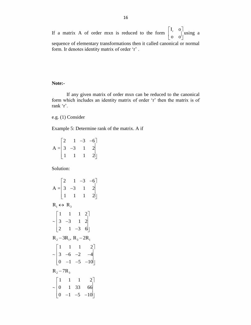
If a matrix A of order mxn is reduced to the form rI o

o o

using a

sequence of elementary transformations then it called canonical or normal

form. Ir denotes identity matrix of order „r‟ .

Note:-

If any given matrix of order mxn can be reduced to the canonical

form which includes an identity matrix of order „r‟ then the matrix is of

rank „r‟.

e.g. (1) Consider

Example 5: Determine rank of the matrix. A if

2 1 3 6

A = 3 3 1 2

1 1 1 2

Solution:

2 1 3 6

A = 3 3 1 2

1 1 1 2

1 3R R

1 1 1 2

3 3 1 2

2 1 3 6

2 1 3 1R 3R , R 2R

1 1 1 2

3 6 2 4

0 1 5 10

2 3R 7R

1 1 1 2

0 1 33 66

0 1 5 10

17

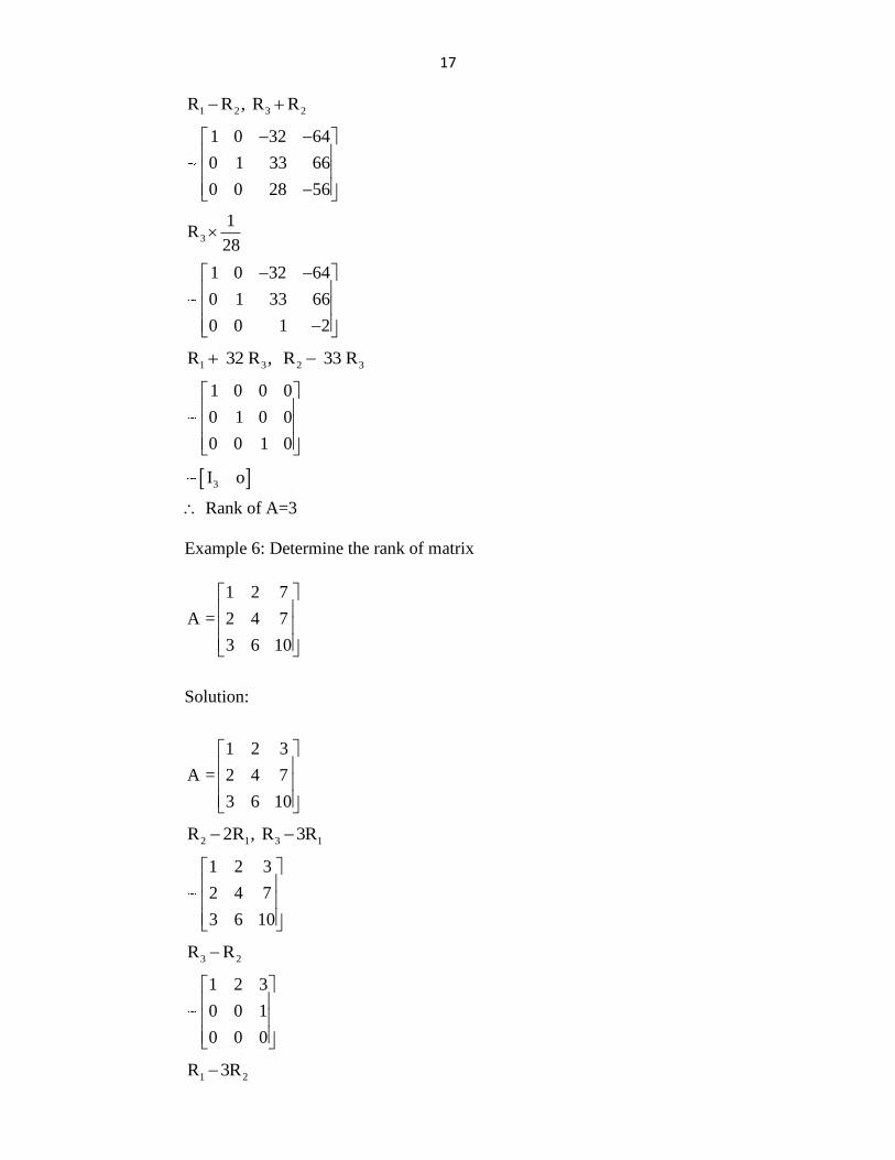
1 2 3 2R R , R R

1 0 32 64

0 1 33 66

0 0 28 56

3

1R

28

1 0 32 64

0 1 33 66

0 0 1 2

1 3 2 3R 32 R , R 33 R

1 0 0 0

0 1 0 0

0 0 1 0

3I o

Rank of A=3

Example 6: Determine the rank of matrix

1 2 7

A = 2 4 7

3 6 10

Solution:

1 2 3

A = 2 4 7

3 6 10

2 1 3 1R 2R , R 3R

1 2 3

2 4 7

3 6 10

3 2R R

1 2 3

0 0 1

0 0 0

1 2R 3R

18

1 2 0

0 0 1

0 0 0

2 1C 2C

1 0 0

0 0 1

0 0 0

1 3C C

1 0 0

0 1 0

0 0 0

2I 0

Rank of A= 2

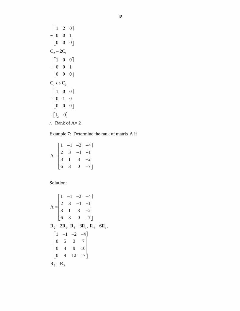
Example 7: Determine the rank of matrix A if

1 1 2 4

2 3 1 1A =

3 1 3 2

6 3 0 7

Solution:

1 1 2 4

2 3 1 1A =

3 1 3 2

6 3 0 7

2 1 3 1 4 1R 2R , R 3R , R 6R ,

1 1 2 4

0 5 3 7

0 4 9 10

0 9 12 17

2 3R R

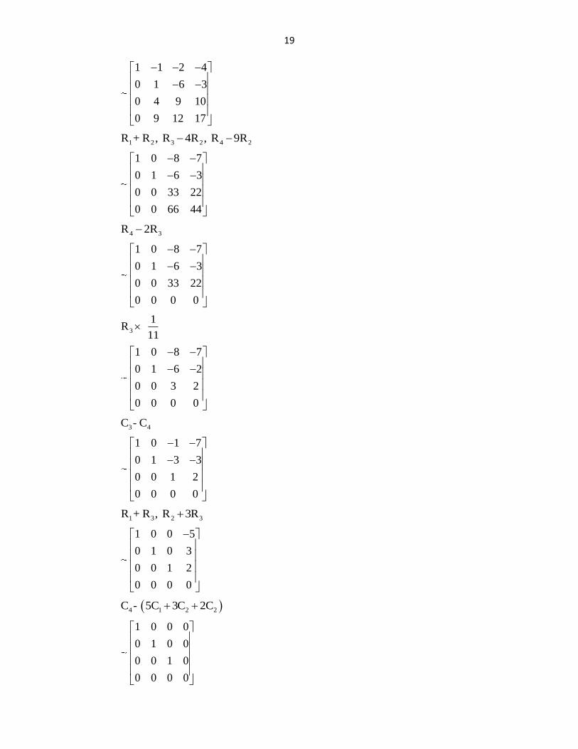
19

1 1 2 4

0 1 6 3

0 4 9 10

0 9 12 17

1 2 3 2 4 2R + R , R 4R , R 9R

1 0 8 7

0 1 6 3

0 0 33 22

0 0 66 44

4 3R 2R

1 0 8 7

0 1 6 3

0 0 33 22

0 0 0 0

3

1R

11

1 0 8 7

0 1 6 2

0 0 3 2

0 0 0 0

3 4C - C

1 0 1 7

0 1 3 3

0 0 1 2

0 0 0 0

1 3 2 3R + R , R 3R

1 0 0 5

0 1 0 3

0 0 1 2

0 0 0 0

4 1 2 2C - 5C 3C 2C

1 0 0 0

0 1 0 0

0 0 1 0

0 0 0 0

20

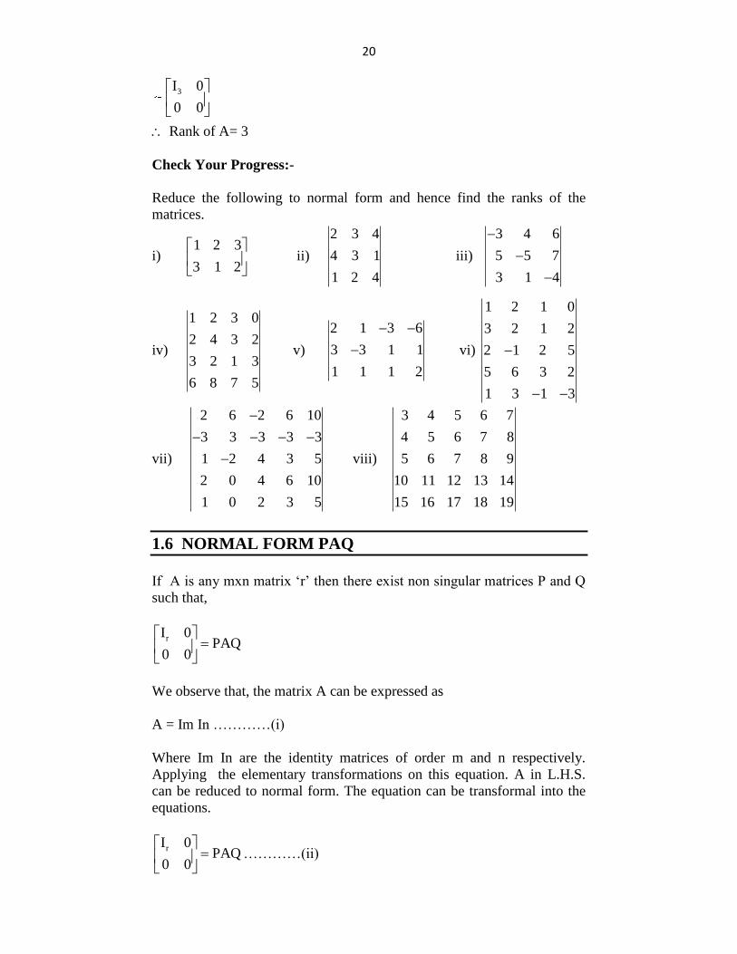
3I 0

0 0

Rank of A= 3

Check Your Progress:-

Reduce the following to normal form and hence find the ranks of the

matrices.

i) 1 2 3

3 1 2

ii)

2 3 4

4 3 1

1 2 4

iii)

3 4 6

5 5 7

3 1 4

iv)

1 2 3 0

2 4 3 2

3 2 1 3

6 8 7 5

v)

2 1 3 6

3 3 1 1

1 1 1 2

vi)

1 2 1 0

3 2 1 2

2 1 2 5

5 6 3 2

1 3 1 3

vii)

2 6 2 6 10

3 3 3 3 3

1 2 4 3 5

2 0 4 6 10

1 0 2 3 5

viii)

3 4 5 6 7

4 5 6 7 8

5 6 7 8 9

10 11 12 13 14

15 16 17 18 19

1.6 NORMAL FORM PAQ

If A is any mxn matrix „r‟ then there exist non singular matrices P and Q

such that,

rI 0PAQ

0 0

We observe that, the matrix A can be expressed as

A = Im In …………(i)

Where Im In are the identity matrices of order m and n respectively.

Applying the elementary transformations on this equation. A in L.H.S.

can be reduced to normal form. The equation can be transformal into the

equations.

rI 0PAQ

0 0

…………(ii)

21

Note that, the row operations can be performed simultaneously on L.H.S.

and prefactor (i.e. Im in equation (i)) and column operations can be

performed simultaneously on L.H.S. and post factor in R.H.S. i.e. [(In in

eqn (i)]

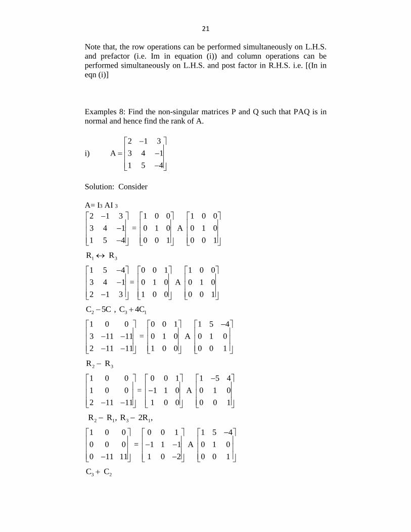
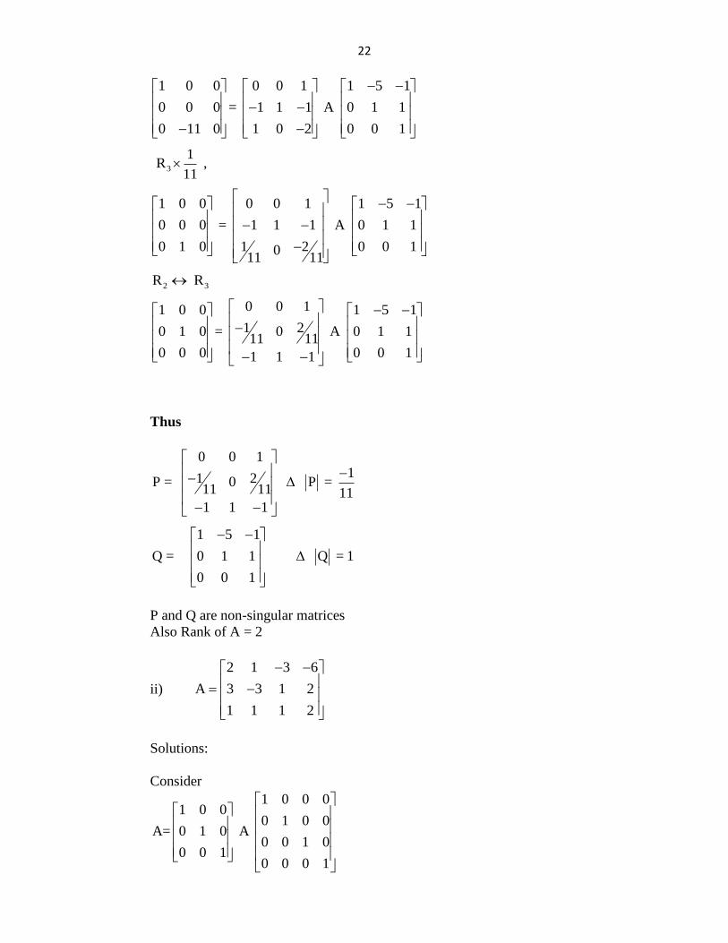
Examples 8: Find the non-singular matrices P and Q such that PAQ is in

normal and hence find the rank of A.

i)

2 1 3

A 3 4 1

1 5 4

Solution: Consider

A= I3 AI 3

2 1 3 1 0 0 1 0 0

3 4 1 = 0 1 0 A 0 1 0

1 5 4 0 0 1 0 0 1

1 3R R

1 5 4 0 0 1 1 0 0

3 4 1 = 0 1 0 A 0 1 0

2 1 3 1 0 0 0 0 1

2 3 1C 5C , C 4C

1 0 0 0 0 1 1 5 4

3 11 11 = 0 1 0 A 0 1 0

2 11 11 1 0 0 0 0 1

2 3R R

1 0 0 0 0 1 1 5 4

1 0 0 = 1 1 0 A 0 1 0

2 11 11 1 0 0 0 0 1

2 1 3 1 R R , R 2R ,

1 0 0 0 0 1 1 5 4

0 0 0 = 1 1 1 A 0 1 0

0 11 11 1 0 2 0 0 1

3 2C C

22

1 0 0 0 0 1 1 5 1

0 0 0 = 1 1 1 A 0 1 1

0 11 0 1 0 2 0 0 1

3

1 R ,

11

1 0 0 0 0 1 1 5 1

0 0 0 = 1 1 1 A 0 1 1

0 1 0 1 2 0 0 1011 11

2 3R R

0 0 11 0 0 1 5 1

1 20 1 0 = 0 A 0 1 111 11

0 0 0 0 0 11 1 1

Thus

0 0 111 2P = 0 P =

11 11 111 1 1

1 5 1

Q = 0 1 1 Q = 1

0 0 1

P and Q are non-singular matrices

Also Rank of A = 2

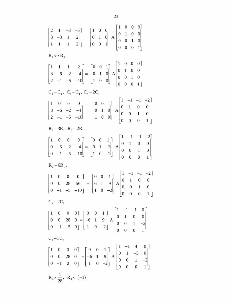
ii)

2 1 3 6

A 3 3 1 2

1 1 1 2

Solutions:

Consider

1 0 0 01 0 0

0 1 0 0A= 0 1 0 A

0 0 1 00 0 1

0 0 0 1

23

1 0 0 02 1 3 6 1 0 0

0 1 0 03 3 1 2 0 1 0 A

0 0 1 01 1 1 2 0 0 1

0 0 0 1

1 3R R

1 0 0 01 1 1 2 0 0 1

0 1 0 03 6 2 4 0 1 0 A

0 0 1 02 1 5 10 1 0 0

0 0 0 1

2 1 3 1 4 1C C , C C , C 2C

1 1 1 21 0 0 0 0 0 1

0 1 0 03 6 2 4 0 1 0 A

0 0 1 02 1 5 10 1 0 0

0 0 0 1

2 1 3 1R 3R , R 2R

1 1 1 21 0 0 0 0 0 1

0 1 0 00 6 2 4 0 1 3 A

0 0 1 00 1 5 10 1 0 2

0 0 0 1

2 3R 6R ,

1 1 1 21 0 0 0 0 0 1

0 1 0 00 0 28 56 6 1 9 A

0 0 1 00 1 5 10 1 0 2

0 0 0 1

4 3C 2C

1 1 1 01 0 0 0 0 0 1

0 1 0 00 0 28 0 6 1 9 A

0 0 1 20 1 5 0 1 0 2

0 0 0 1

3 2C 5C

1 1 4 01 0 0 0 0 0 1

0 1 5 00 0 28 0 6 1 9 A

0 0 1 20 1 0 0 1 0 2

0 0 0 1

2 3

1R , R 1

28

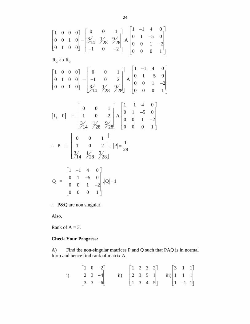
24

1 1 4 00 0 11 0 0 0

0 1 5 03 910 0 1 0 A 14 28 28 0 0 1 2

0 1 0 0 1 0 20 0 0 1

2 3R R

1 1 4 01 0 0 0 0 0 1

0 1 5 00 1 0 0 1 0 2 A

0 0 1 20 0 1 0 3 91

0 0 0 114 28 28

3

1 1 4 00 0 1

0 1 5 0I 0 = 1 0 2 A

0 0 1 23 91

0 0 0 114 28 28

0 0 11

P = 1 0 2 , P28

3 9114 28 28

1 1 4 0

0 1 5 0Q = , Q 1

0 0 1 2

0 0 0 1

P&Q are non singular.

Also,

Rank of A = 3.


A) Find the non-singular matrices P and Q such that PAQ is in normal

form and hence find rank of matrix A.

i)

1 0 2

2 3 4

3 3 6

ii)

1 2 3 2

2 3 5 1

1 3 4 5

iii)

3 1 1

1 1 1

1 1 1

25

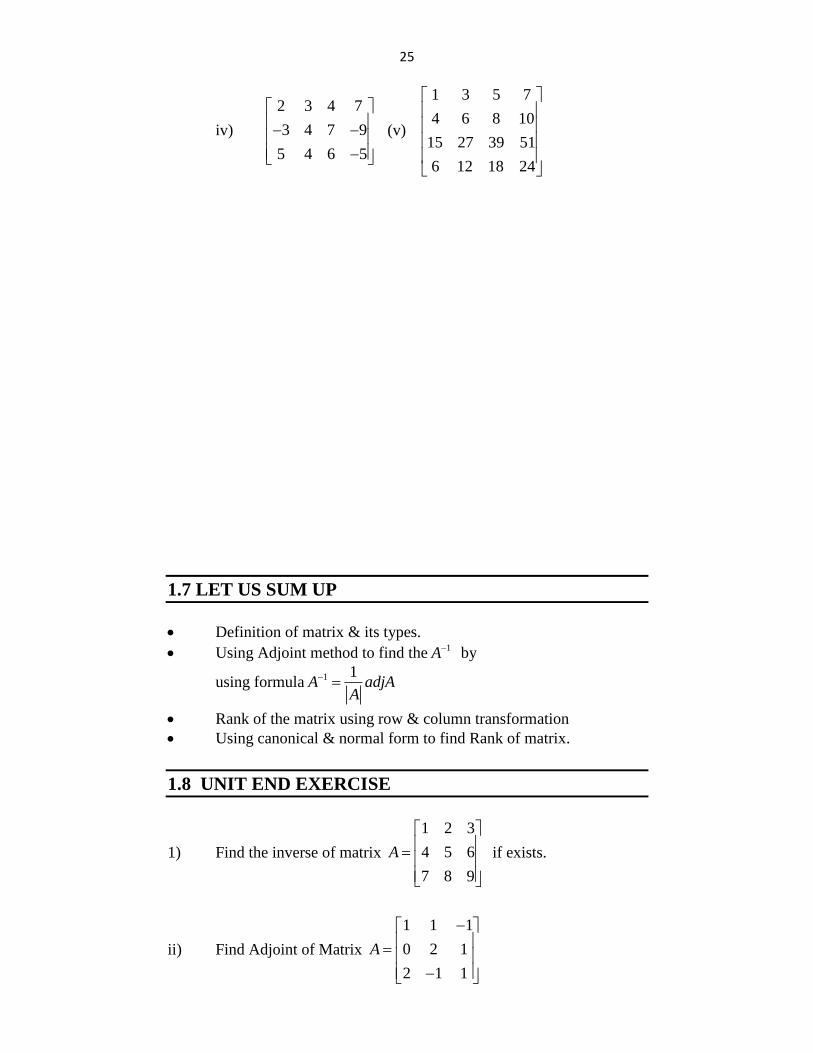
iv)

2 3 4 7

3 4 7 9

5 4 6 5

(v)

1 3 5 7

4 6 8 10

15 27 39 51

6 12 18 24

1.7 LET US SUM UP

Definition of matrix & its types.

Using Adjoint method to find the 1A by

using formula 1 1A adjA

A

Rank of the matrix using row & column transformation

Using canonical & normal form to find Rank of matrix.

1.8 UNIT END EXERCISE

1) Find the inverse of matrix

1 2 3

4 5 6

7 8 9

A

if exists.

ii) Find Adjoint of Matrix

1 1 1

0 2 1

2 1 1

A

26

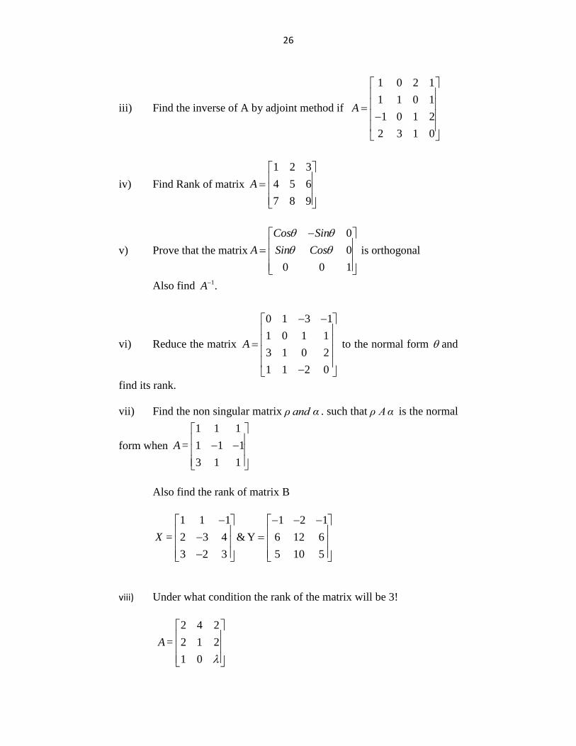
iii) Find the inverse of A by adjoint method if

1 0 2 1

1 1 0 1

1 0 1 2

2 3 1 0

A

iv) Find Rank of matrix

1 2 3

4 5 6

7 8 9

A

v) Prove that the matrix

0

0

0 0 1

Cos Sin

A Sin Cos

is orthogonal

Also find

1.A

vi) Reduce the matrix

0 1 3 1

1 0 1 1

3 1 0 2

1 1 2 0

A

to the normal form and

find its rank.

vii) Find the non singular matrix ρ and α . such that ρ A α is the normal

form when

1 1 1

1 1 1

3 1 1

A =

Also find the rank of matrix B

1 1 1 1 2 1

2 3 4 & Y 6 12 6

3 2 3 5 10 5

X =

viii) Under what condition the rank of the matrix will be 3!

2 4 2

2 1 2

1 0

A =

27

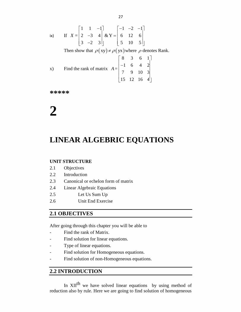
ix) If

1 1 1 1 2 1

2 3 4 & Y 6 12 6

3 2 3 5 10 5

X =

Then show that xy yx where denotes Rank.

x) Find the rank of matrix

8 3 6 1

1 6 4 2

7 9 10 3

15 12 16 4

A =

*****

2

LINEAR ALGEBRIC EQUATIONS

UNIT STRUCTURE

2.1 Objectives

2.2 Introduction

2.3 Canonical or echelon form of matrix

2.4 Linear Algebraic Equations

2.5 Let Us Sum Up


2.1 OBJECTIVES

After going through this chapter you will be able to

- Find the rank of Matrix.

- Find solution for linear equations.

- Type of linear equations.

- Find solution for Homogeneous equations.

- Find solution of non-Homogeneous equations.

2.2 INTRODUCTION

In XIIth we have solved linear equations by using method of

reduction also by rule. Here we are going to find solution of homogeneous

28

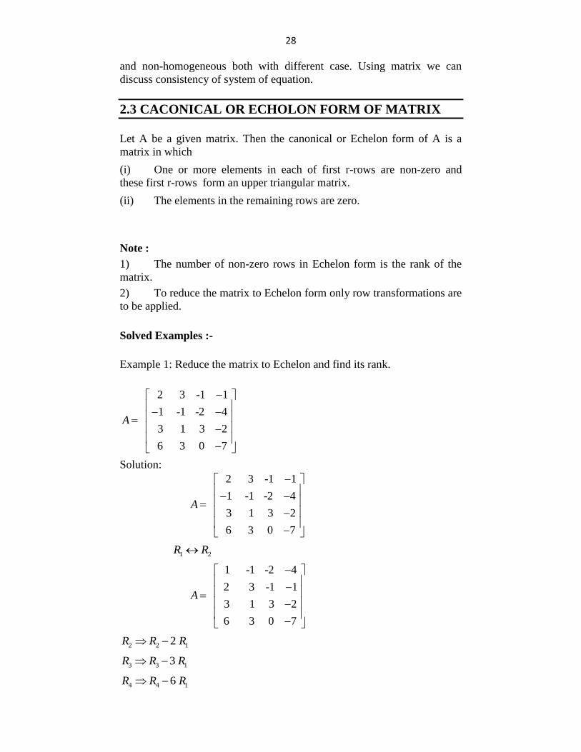
and non-homogeneous both with different case. Using matrix we can

discuss consistency of system of equation.

2.3 CACONICAL OR ECHOLON FORM OF MATRIX

Let A be a given matrix. Then the canonical or Echelon form of A is a

matrix in which

(i) One or more elements in each of first r-rows are non-zero and

these first r-rows form an upper triangular matrix.

(ii) The elements in the remaining rows are zero.

Note :

1) The number of non-zero rows in Echelon form is the rank of the

matrix.

2) To reduce the matrix to Echelon form only row transformations are

to be applied.

Solved Examples :-

Example 1: Reduce the matrix to Echelon and find its rank.

2 3 -1 1

1 -1 -2 4

3 1 3 2

6 3 0 7

A

Solution:

2 3 -1 1

1 -1 -2 4

3 1 3 2

6 3 0 7

A

1 2 R R

1 -1 -2 4

2 3 -1 1

3 1 3 2

6 3 0 7

A

2 2 12 R R R

3 3 13 R R R

4 4 16 R R R

29

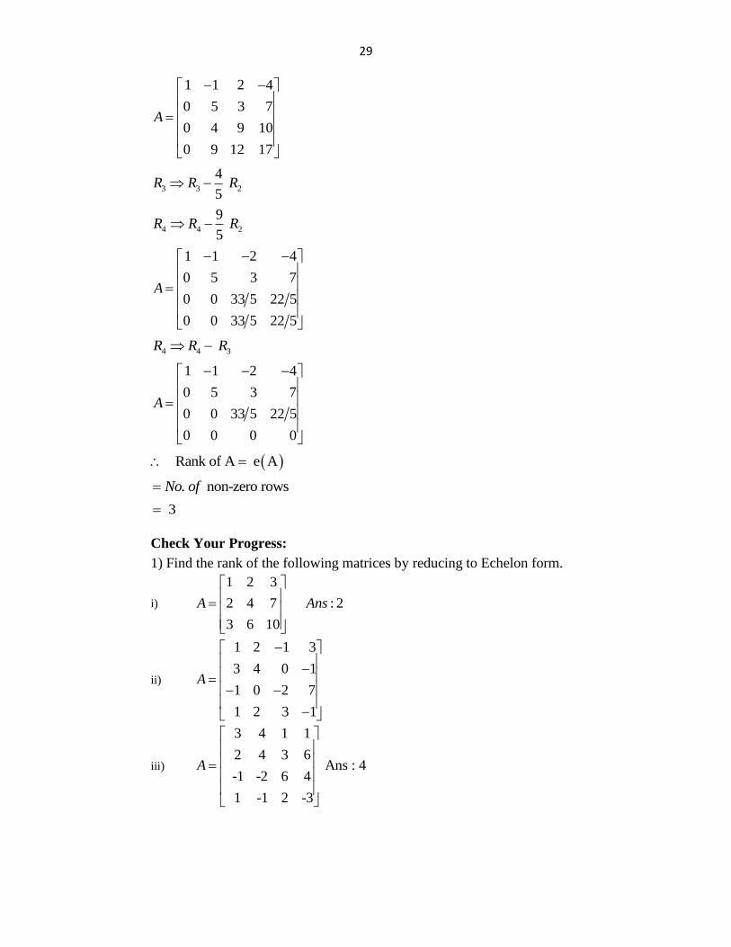
1 1 2 4

0 5 3 7

0 4 9 10

0 9 12 17

A

3 3 2

4

5R R R

4 4 2

9

5R R R

1 1 2 4

0 5 3 7

0 0 33 5 22 5

0 0 33 5 22 5

A

4 4 3 R R R

1 1 2 4

0 5 3 7

0 0 33 5 22 5

0 0 0 0

A

Rank of A e A

. non-zero rowsNo of

3


1) Find the rank of the following matrices by reducing to Echelon form.

i)

1 2 3

2 4 7 : 2

3 6 10

A Ans

ii)

1 2 1 3

3 4 0 1

1 0 2 7

1 2 3 1

A

iii)

3 4 1 1

2 4 3 6 Ans : 4-1 -2 6 4

1 -1 2 -3

A

30

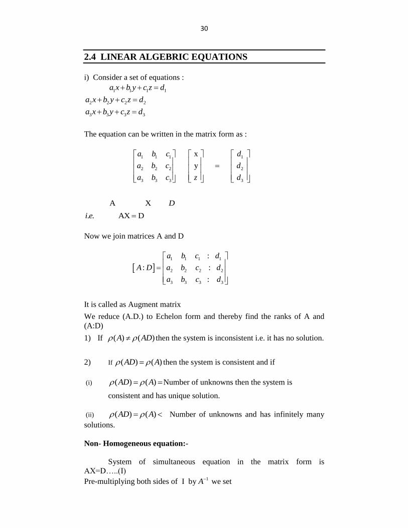
2.4 LINEAR ALGEBRIC EQUATIONS

i) Consider a set of equations :

1 1 1 1a x b y c z d

2 2 2 2a x b y c z d

3 3 3 3a x b y c z d

The equation can be written in the matrix form as :

1 1 1 1

2 2 2 2

3 3 3 3

x

y

a b c d

a b c d

a b c z d

A X D

. . AX Di e

Now we join matrices A and D

1 1 1 1

2 2 2 2

3 3 3 3

:

: :

:

a b c d

A D a b c d

a b c d

It is called as Augment matrix

We reduce (A.D.) to Echelon form and thereby find the ranks of A and

(A:D)

1) If ( ) ( )A AD then the system is inconsistent i.e. it has no solution.

2) If ( ) ( )AD A then the system is consistent and if

(i) ( ) ( )AD A Number of unknowns then the system is

consistent and has unique solution.

(ii)

( ) ( )AD A Number of unknowns and has infinitely many

solutions.

Non- Homogeneous equation:-

System of simultaneous equation in the matrix form is

AX=D…..(I)

Pre-multiplying both sides of I by 1A we set

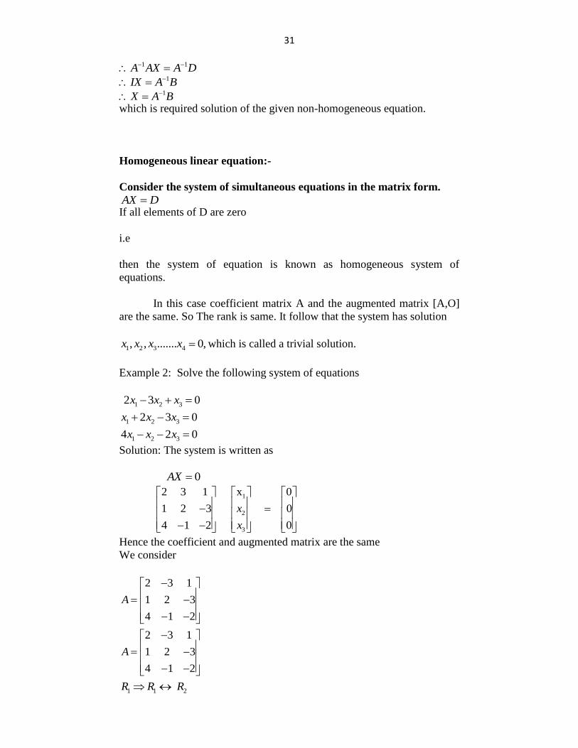
31

1 1A AX A D

1IX A B

1X A B

which is required solution of the given non-homogeneous equation.

Homogeneous linear equation:-

Consider the system of simultaneous equations in the matrix form.

AX D

If all elements of D are zero

i.e

then the system of equation is known as homogeneous system of

equations.

In this case coefficient matrix A and the augmented matrix [A,O]

are the same. So The rank is same. It follow that the system has solution

1 2 3 4, , ....... 0,x x x x which is called a trivial solution.

Example 2: Solve the following system of equations

1 2 32 3 0x x x

1 2 32 3 0x x x

1 2 34 2 0x x x

Solution: The system is written as

0AX

1

2

3

2 3 1 x 0

1 2 3 0

4 1 2 0

x

x

Hence the coefficient and augmented matrix are the same

We consider

2 3 1

1 2 3

4 1 2

A

2 3 1

1 2 3

4 1 2

A

1 1 2 R R R

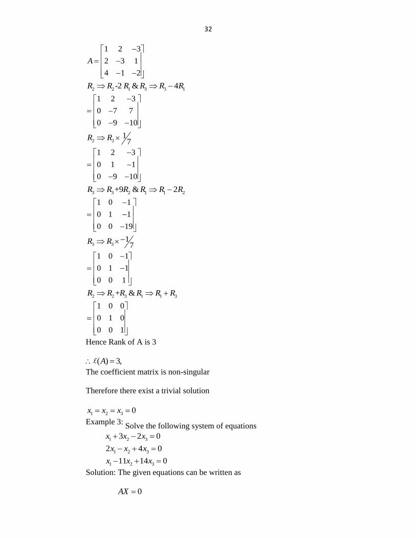
32

1 2 3

2 3 1

4 1 2

A

2 2 1 3 3 1-2 & 4R R R R R R

1 2 3

0 7 7

0 9 10

2 21

7R R

1 2 3

0 1 1

0 9 10

3 3 2 1 1 2+9 & 2R R R R R R

1 0 1

0 1 1

0 0 19

3 31

7R R

1 0 1

0 1 1

0 0 1

2 2 3 1 1 3+ &R R R R R R

1 0 0

0 1 0

0 0 1

Hence Rank of A is 3

( ) 3,A

The coefficient matrix is non-singular

Therefore there exist a trivial solution

1 2 3 0x x x

Example 3: Solve the following system of equations

1 2 33 2 0x x x

1 2 32 4 0x x x

1 2 311 14 0x x x

Solution: The given equations can be written as

0AX

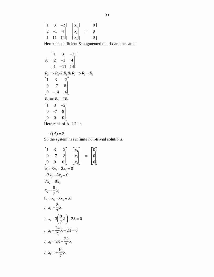
33

1

2

3

1 3 2 x 0

2 1 4 0

1 11 14 0

x

x

Here the coefficient & augmented matrix are the same

1 3 2

2 1 4

1 11 14

A

2 2 1 3 3 1-2 &R R R R R R

1 3 2

0 7 8

0 14 16

3 3 22R R R

1 3 2

0 7 8

0 0 0

Here rank of A is 2 i.e

( ) 2A

So the system has infinite non-trivial solutions.

1

2

3

1 3 2 x 0

0 7 8 0

0 0 0 0

x

x

1 2 33 2 0x x x

2 37 8 0x x

2 37 8x x

2 3

8

7x x

Let 3 38x x

2

8

7x

1

83 2 0

7x

1

242 0

7x

1

242

7x

1

10

7x

34

Hence 1

10

7x

2

8

7x and 3x

1

2

3

10

7x8

7

x

x

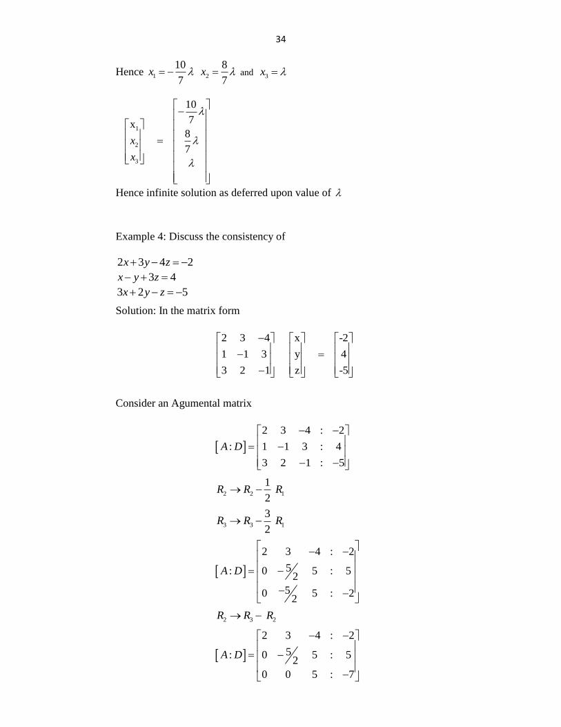
Hence infinite solution as deferred upon value of

Example 4: Discuss the consistency of

2 3 4 2x y z

3 4x y z

3 2 5x y z

Solution: In the matrix form

2 3 4 x -2

1 1 3 y 4

3 2 1 z -5

Consider an Agumental matrix

2 3 4 : 2

: 1 1 3 : 4

3 2 1 : 5

A D

2 2 1

1

2R R R

3 3 1

3

2R R R

2 3 4 : 2

5: 0 5 : 52

50 5 : 22

A D

2 3 2 R R R

2 3 4 : 2

5: 0 5 : 52

0 0 5 : 7

A D

35

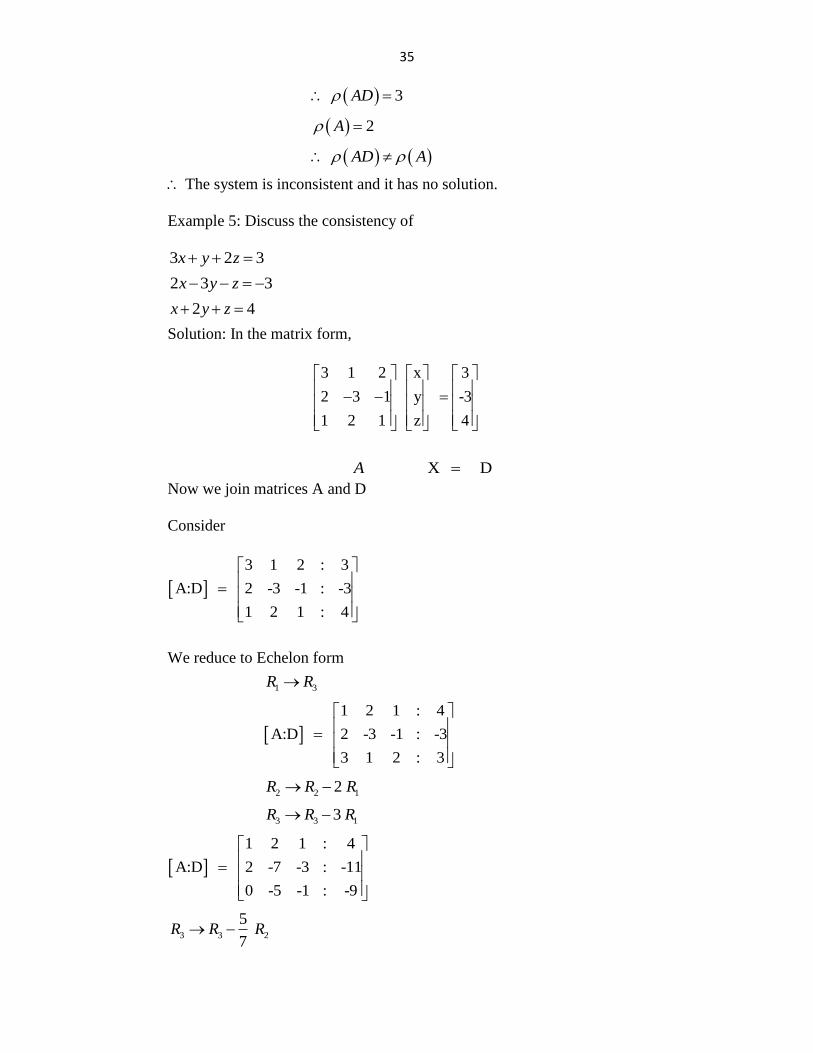
3AD

2A

AD A

The system is inconsistent and it has no solution.

Example 5: Discuss the consistency of

3 2 3x y z

2 3 3x y z

2 4x y z

Solution: In the matrix form,

3 1 2 x 3

2 3 1 y -3

1 2 1 z 4

X DA

Now we join matrices A and D

Consider

3 1 2 : 3

A:D 2 -3 -1 : -3

1 2 1 : 4

We reduce to Echelon form

1 3R R

1 2 1 : 4

A:D 2 -3 -1 : -3

3 1 2 : 3

2 2 12 R R R

3 3 13 R R R

1 2 1 : 4

A:D 2 -7 -3 : -11

0 -5 -1 : -9

3 3 2

5

7R R R

36

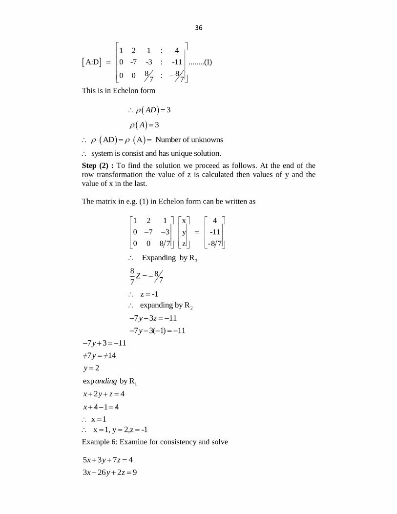
1 2 1 : 4

A:D 0 -7 -3 : -11 ........(1)

8 80 0 :7 7

This is in Echelon form

3AD

3A

AD A Number of unknowns

system is consist and has unique solution.

Step (2) : To find the solution we proceed as follows. At the end of the

row transformation the value of z is calculated then values of y and the

value of x in the last.

The matrix in e.g. (1) in Echelon form can be written as

1 2 1 x 4

0 7 3 y -11

0 0 8 7 z -8 7

3 Expanding by R

8 8

77Z

z -1

2 expanding by R

7 3 11y z

7 3( 1) 11y

7 3 11y

7 14y

2y

1exp by Randing

2 4x y z

4 1 4x

x 1

x 1, y 2,z -1

Example 6: Examine for consistency and solve

5 3 7 4x y z

3 26 2 9x y z

37

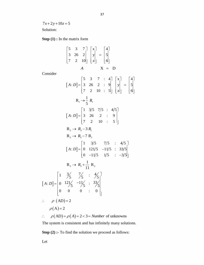
7 2 10 5x y z

Solution:

Step (1) : In the matrix form

5 3 7 x 4

3 26 2 y 5

7 2 10 z 6

X DA

Consider

5 3 7 : 4 x 4

: 3 26 2 : 9 y 5

7 2 10 : 5 z 6

A D

1 1

1 R

5R

1 3 5 7 5 : 4 5

: 3 26 2 : 9

7 2 10 : 5

A D

2 2 1R 3 R R

3 3 1R 7 RR

1 3 5 7 5 : 4 5

: 0 121 5 11 5 : 33 5

0 11 5 1 5 : 3 5

A D

3 3 2

1R R

11R

3 7 41 :5 5 5

33121 11: 0 :5 5 5

0 0 0 : 0

A D

AD 2

A 2

AD 2 3 of unknownsA Number

The system is consistent and has infinitely many solutions.

Step (2) :- To find the solution we proceed as follows:

Let

38

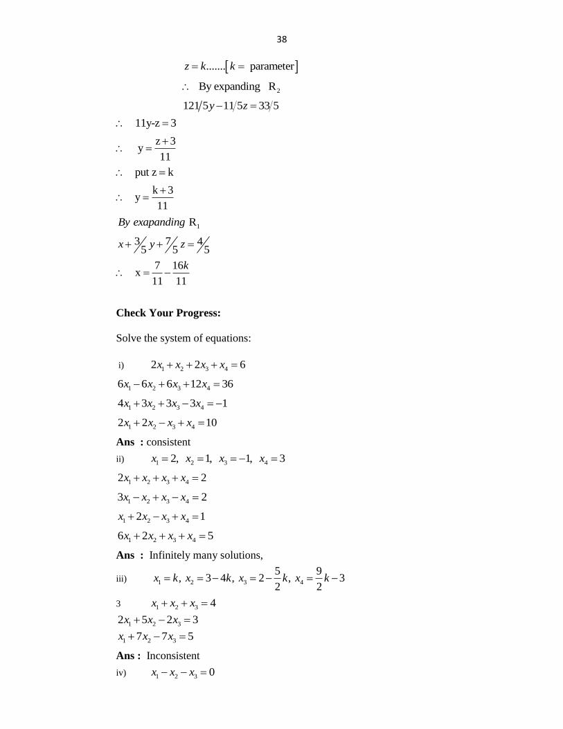
....... parameterz k k

2 By expanding R

121 5 11 5 33 5 y z

11y-z 3

z 3 y

11

put z k

k 3 y

11

1 RBy exapanding

3 7 45 5 5

x y z

7 16 x

11 11

k


Solve the system of equations:

i) 1 2 3 42 2 6x x x x

1 2 3 46 6 6 12 36x x x x

1 2 3 44 3 3 3 1x x x x

1 2 3 42 2 10x x x x

Ans : consistent

ii) 1 2 3 42, 1, 1, 3x x x x

1 2 3 42 2x x x x

1 2 3 43 2x x x x

1 2 3 42 1x x x x

1 2 3 46 2 5x x x x

Ans : Infinitely many solutions,

iii) 1 2 3 4

5 9, 3 4 , 2 , 3

2 2x k x k x k x k

3 1 2 3 4x x x

1 2 32 5 2 3x x x

1 2 37 7 5x x x

Ans : Inconsistent

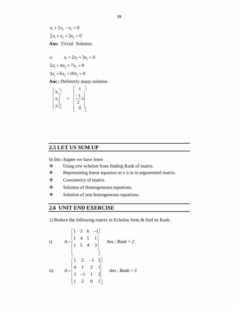
iv) 1 2 3 0x x x

39

1 2 32 0x x x

1 2 32 3 0x x x

Ans: Trivial Solution.

v) 1 2 32 3 0x x x

1 2 32 4 7 0x x x

1 2 33 6 10 0x x x

Ans : Definitely many solution

1

2

3

x1

2

0

x

x

2.5 LET US SUM UP

In this chapter we have learn

Using row echelon from finding Rank of matrix.

Representing linear equation m x n in to argumented matrix.

Consistency of matrix.

Solution of Homogeneous equations.

Solution of non homogeneous equations.


1) Reduce the following matrix in Echolon form & find its Rank.

i)

1 3 6 1

1 4 5 1

1 5 4 3A Ans : Rank = 2

ii)

1 2 1 3

4 1 2 1

3 1 1 2

1 2 0 1

A Ans : Rank = 3

40

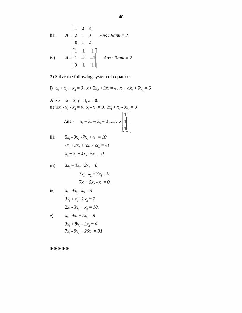
iii)

1 2 3

2 1 0

0 1 2

A Ans : Rank = 2

iv)

1 1 1

1 1 1

3 1 1

A Ans : Rank = 2

2) Solve the following system of equations.

i) 1 2 3 2 3 1 2 3x + x + x = 3, x+2x +3x = 4, x +4x +9x = 6

Ans:- 2, 1, 0.x y z

ii) 1 2 3 1 3 1 2 32x - x - x = 0, x - x = 0, 2x + x - 3x = 0

Ans:- 1 2 3

1

..... 1 .

1

x x x

.

iii) 1 2 3 45x - 3x -7x + x = 10

1 2 3 4-x +2x +6x - 3x = -3

1 2 3 4x + x +4x - 5x = 0

iii) 1 2 32x +3x - 2x = 0

1 2 33x - x +3x = 0

1 2 37x +5x - x = 0.

iv) 1 2 3x - 4x - x = 3

1 2 33x + x - 2x =7

1 2 32x - 3x + x = 10.

v) 1 2 3x - 4x +7x = 8

1 2 33x +8x - 2x = 6

1 2 37x - 8x +26x = 31

*****

41

3 LINEAR DEPENDANCE AND

INDEPENDANCE

OF VECTORS

UNIT STRUCTURE

3.1 Objectives

3.2 Introduction

3.3 Definitions

3.4 The Inner Product

3.5 Eigen Values and Eigen Vectors

3.6 Summary


3.1 Objectives

After going through this chapter you will able to

Find linearly independent & linearly dependent vector.

Inner product of two vector

Find characteristic equation of matrix

Find the of characteristic equation i.e

Find the corresponding .Eigen vector to Eigen value.

3.2 Introduction

In this chapter we are going to discuss linearly dependent &

independent also. Inner two vector using the characteristic equation of

matrix. We are going to evaluate .Eigen value & Eigen.vector of matrix A.

Vector :- An set of n elements written as 1 2 3 4, , , ,............. nx x x x x xis

called a vector of n-dimensions.

Note : Any two or column matrix is called as a vector and numbers are

called as scalars.

3.3 Definitions

Linearly Independent Vector

Let

1 2 , ,............. be n vectors of some ordernLet x x x

42

1 1 2 2 nLet c c ........... c 0nx x x

1 2 c , , ...... are scalars. Where c

1 2 nIf (i) c .............. c 0 thenc

1 2 x , , ........ are linearly independentnx x

i 1 2and (ii) if not all c are zero then , ,.......... nx x x

are linearly dependent

1 2If x , ,......... are linearly dependent then a relation existsnx x

between them which can be found out

Solved examples:-

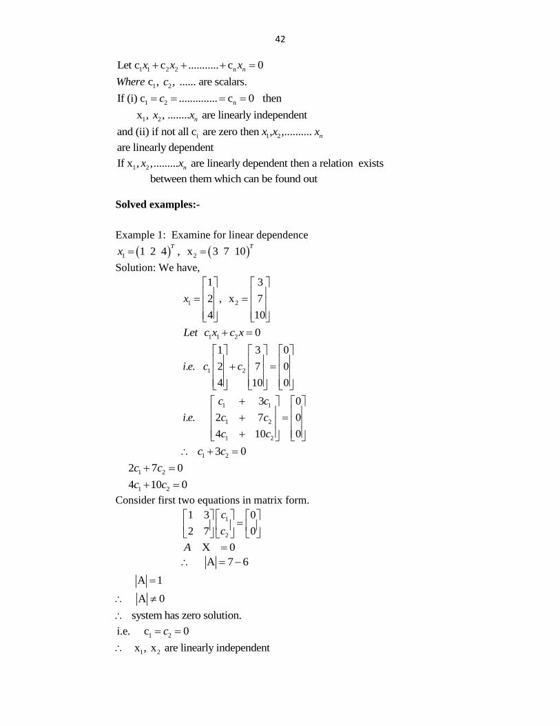
Example 1: Examine for linear dependence

1 21 2 4 , x 3 7 10T T

x

Solution: We have,

1 2

1 3

2 , x 7

4 10

x

1 1 2 0Let c x c x

1 2

1 3 0

. . 2 7 0

4 10 0

i e c c

1 1

1 2

1 2

3 0

. . 2 7 0

4 10 0

c c

i e c c

c c

1 2 3 0c c

1 2 2 7 0c c

1 2 4 10 0c c

Consider first two equations in matrix form.

1

2

1 3 0

2 7 0

c

c

X 0A

A 7 6

A 1

A 0

system has zero solution.

1 2i.e. c 0c

1 2 x , x are linearly independent

43

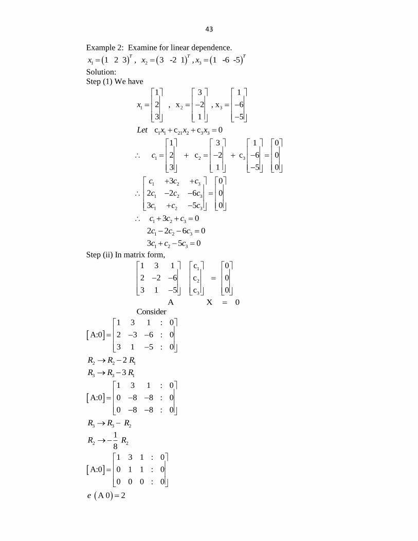
Example 2: Examine for linear dependence.

1 2 31 2 3 , 3 -2 1 , 1 -6 -5T T T

x x x

Solution:

Step (1) We have

1 2 3

1 3 1

2 , x 2 , x 6

3 1 5

x

1 1 21 2 3 3 c c c 0Let x x x

1 2 3

1 3 1 0

2 c 2 c 6 0

3 1 5 0

c

1 2 3

1 2 3

1 2 3

3 0

2 2 6 0

3 5 0

c c c

c c c

c c c

1 2 3 3 0c c c

1 2 3 2 2 6 0c c c

1 2 3 3 5 0c c c

Step (ii) In matrix form,

1

2

3

1 3 1 c 0

2 2 6 c 0

3 1 5 c 0

A X 0

Consider

1 3 1 : 0

A:0 2 3 6 : 0

3 1 5 : 0

2 2 12 R R R

3 3 13 R R R

1 3 1 : 0

A:0 0 8 8 : 0

0 8 8 : 0

3 3 2 R R R

2 2

1

8R R

1 3 1 : 0

A:0 0 1 1 : 0

0 0 0 : 0

A 0 2e

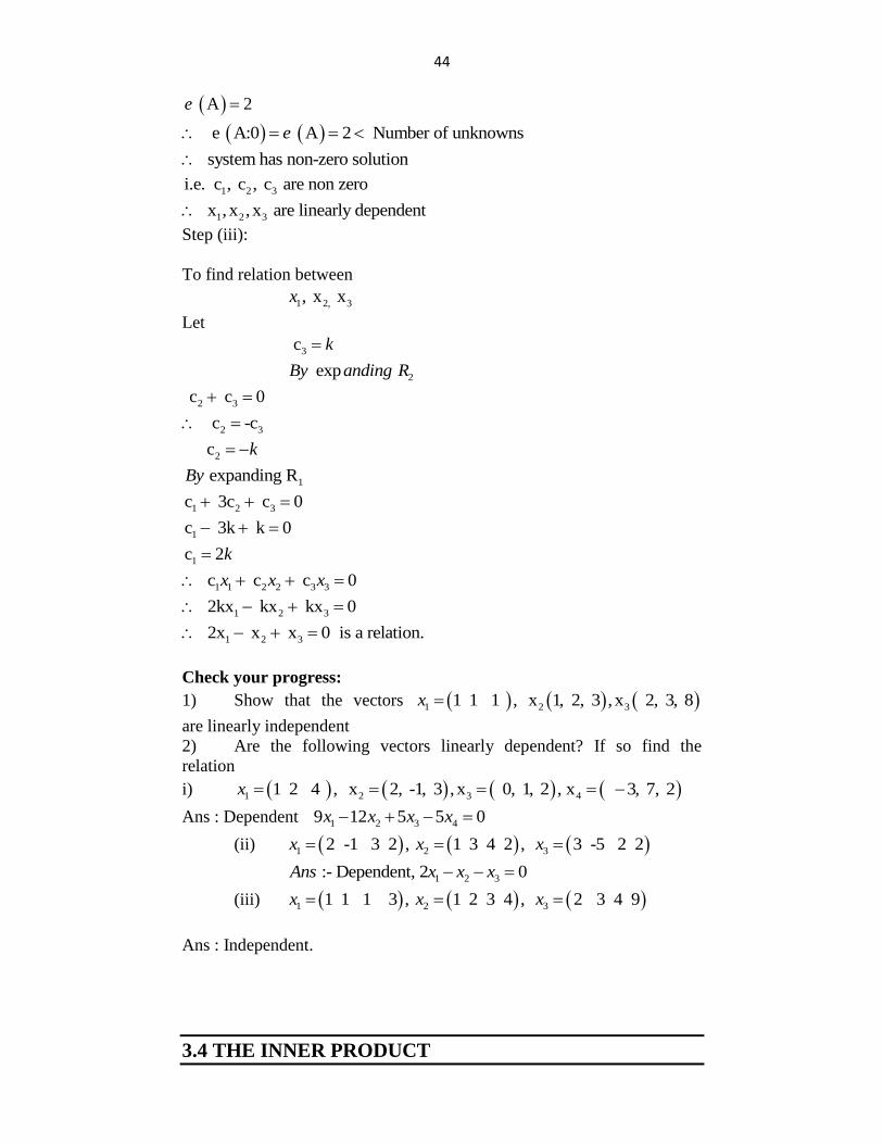
44

A 2e

e A:0 A 2 Number of unknownse

system has non-zero solution

1 2 3i.e. c , c , c are non zero

1 2 3 x , x ,x are linearly dependent

Step (iii):

To find relation between

1 2, 3, x xx

Let

3 c k

2 exp By anding R

2 3 c c 0

2 3 c -c

2 c k

1 expanding RBy

1 2 3c 3c c 0

1c 3k k 0

1c 2k

1 1 2 2 3 3 c c c 0x x x

1 2 3 2kx kx kx 0

1 2 3 2x x x 0 is a relation.

Check your progress:

1) Show that the vectors 1 2 31 1 1 , x 1, 2, 3 ,x 2, 3, 8x

are linearly independent

2) Are the following vectors linearly dependent? If so find the

relation

i) 1 2 3 41 2 4 , x 2, -1, 3 ,x 0, 1, 2 , x 3, 7, 2x

Ans : Dependent 1 2 3 49 12 5 5 0x x x x

(ii) 1 2 32 -1 3 2 , 1 3 4 2 , 3 -5 2 2x x x

1 2 3 :- Dependent, 2 0Ans x x x

(iii) 1 2 31 1 1 3 , 1 2 3 4 , 2 3 4 9x x x

Ans : Independent.

3.4 THE INNER PRODUCT

45

If 1 2( , ....... )nX x x x and

1 2( , ....... )nY y y y

then<X,Y> denotes inner product

1 1 2 2 3 3, ........ n nX Y x y x y x y x y is in inner product of X and Y.

Let V be a vector space and X,Y V then<X,Y> it said to be an inner

product if it satisfies following properties.

i) <X,Y> =0

ii) <X,Y> = <Y,X>

iii) <X,Y+Z> = <X,Y> + <X,Z>

iv) <X, Y> = <X,Y> where is scalar.

v) <X,Y> = 0 if and only if X=0.

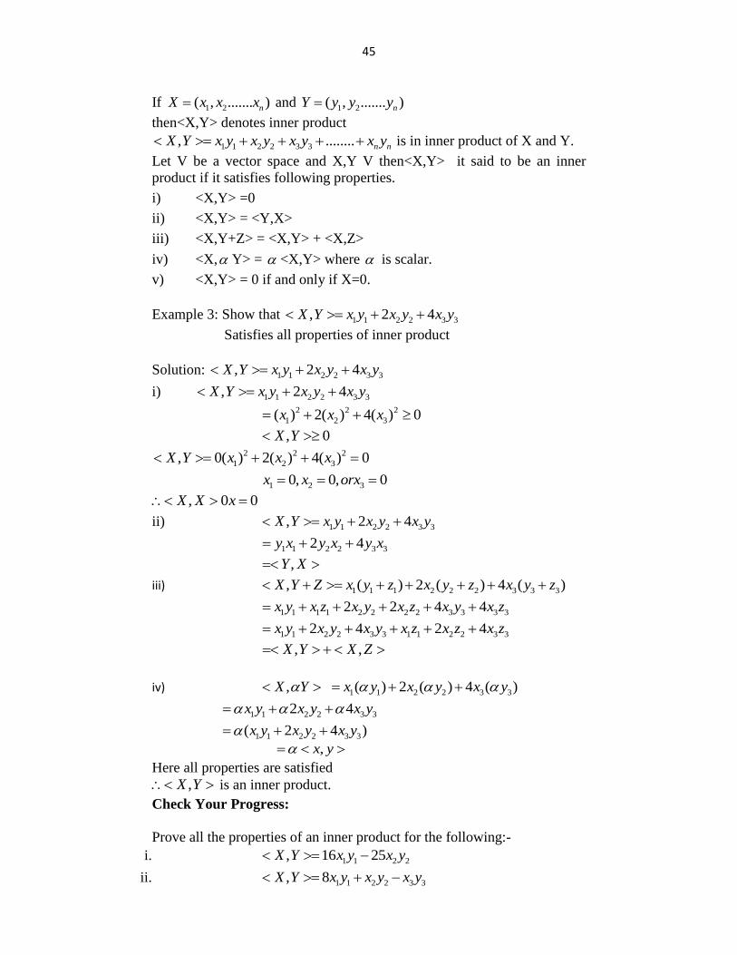
Example 3: Show that 1 1 2 2 3 3, 2 4X Y x y x y x y

Satisfies all properties of inner product

Solution: 1 1 2 2 3 3, 2 4X Y x y x y x y

i) 1 1 2 2 3 3, 2 4X Y x y x y x y

2 2 2

1 2 3( ) 2( ) 4( ) 0x x x

, 0X Y

2 2 2

1 2 3, 0( ) 2( ) 4( ) 0X Y x x x

1 2 30, 0, 0x x orx

, 0 0X X x

ii) 1 1 2 2 3 3, 2 4X Y x y x y x y

1 1 2 2 3 32 4y x y x y x

,Y X

iii) 1 1 1 2 2 2 3 3 3, ( ) 2 ( ) 4 ( )X Y Z x y z x y z x y z

1 1 1 1 2 2 2 2 3 3 3 32 2 4 4x y x z x y x z x y x z

1 1 2 2 3 3 1 1 2 2 3 32 4 2 4x y x y x y x z x z x z

, ,X Y X Z

iv) 1 1 2 2 3 3, ( ) 2 ( ) 4 ( )X Y x y x y x y

1 1 2 2 3 32 4x y x y x y

1 1 2 2 3 3( 2 4 )x y x y x y

,x y

Here all properties are satisfied

,X Y is an inner product.


Prove all the properties of an inner product for the following:-

i. 1 1 2 2, 16 25X Y x y x y

ii. 1 1 2 2 3 3, 8X Y x y x y x y

46

iii. 1 1 2 2 3 3, 3 4X Y x y x y x y

iv. , ( ). ( ).b

a

f g f t g t dt

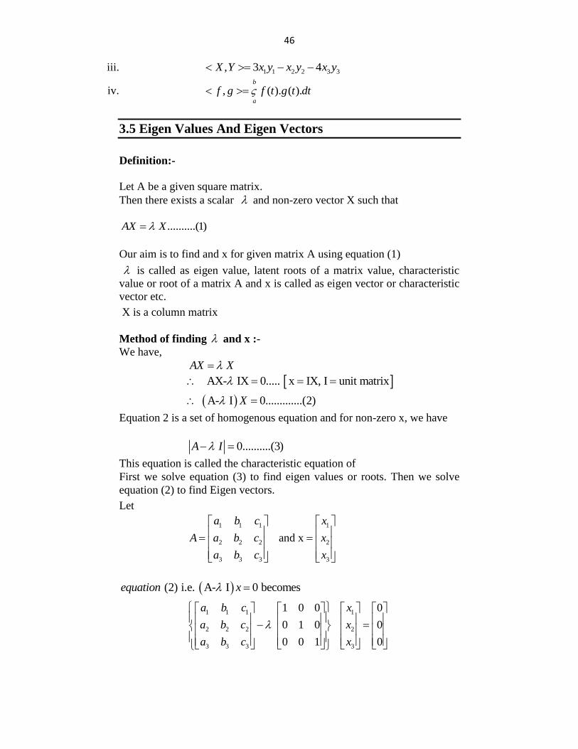
3.5 Eigen Values And Eigen Vectors

Definition:-

Let A be a given square matrix.

Then there exists a scalar and non-zero vector X such that

..........(1)AX X

Our aim is to find and x for given matrix A using equation (1)

is called as eigen value, latent roots of a matrix value, characteristic

value or root of a matrix A and x is called as eigen vector or characteristic

vector etc.

X is a column matrix

Method of finding and x :-

We have,

AX X

AX- IX 0..... x IX, I unit matrix

A- I 0.............(2)X

Equation 2 is a set of homogenous equation and for non-zero x, we have

0..........(3)A I

This equation is called the characteristic equation of

First we solve equation (3) to find eigen values or roots. Then we solve

equation (2) to find Eigen vectors.

Let

1 1 1 1

2 2 2 2

3 3 3 3

and x

a b c x

A a b c x

a b c x

(2) i.e. A- I 0 becomesequation x

1 1 1 1

2 2 2 2

3 3 3 3

1 0 0 0

0 1 0 0

0 0 1 0

a b c x

a b c x

a b c x

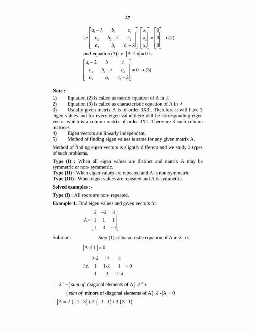
47

1 1 1 1

2 2 2 2

3 3 3 3

0

. . 0 (2)

0

a b c x

i e a b c x

a b c x

equation (3) i.e. A- x 0 isand

1 1 1

2 2 2

3 3 3

0 (3)

a b c

a b c

a b c

Note :

1) Equation (2) is called as matrix equation of A in

2) Equation (3) is called as characteristic equation of A in

3) Usually given matrix A is of order 3X3 . Therefore it will have 3

eigen values and for every eigen value there will be corresponding eigen

vector which is a column matrix of order 3X1. There are 3 such column

matrices.

4) Eigen vectors are linearly independent.

5) Method of finding eigen values is same for any given matrix A.

Method of finding eigen vectors is slightly different and we study 3 types

of such problems.

Type (I) : When all eigen values are distinct and matrix A may be

symmetric or non- symmetric.

Type (II) : When eigen values are repeated and A is non-symmetric

Type (III) : When eigen values are repeated and A is symmetric.

Solved examples :-

Type (I) : All roots are non- repeated.

Example 4: Find eigen values and given vectors for

2 2 3

1 1 1

1 3 1

A

Solution: (1) : Charactristic equation of A in i s Step

A- I 0

2- -2 3

. . 1 1- 1 0

1 3 -1-

i e

3 2 diagonal elements of A sum of

minors of diagonal elements of A - A 0sum of

2 1 3 2 1 1 3 3 1A

48

-8-4 6

A 6

Characteristic equation is given by

3 2 2 4 5 4 - 6 0

3 2 2 -5 6 0

sin sum of coefficient 0ce

-1 is a factor.

Synthetic division: 1 1 -2 -5 6

1 -1 -6

1 -1 -6 0

2 -1 6 0

-1 -3 2 0

1, -2, 3

The roots are non- repeated

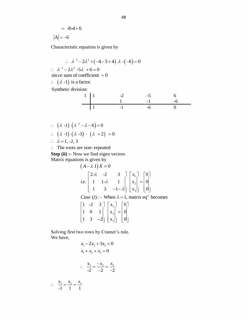
Step (ii) :- Now we find eigen vectors

Matrix equations is given by

I 0A X

1

2

3

2- -2 3 x 0

. . 1 1- 1 x 0

1 3 1 x 0

i e

n ( ) : When 1, matrix eq becomes Case i

1

2

3

1 -2 3 x 0

1 0 1 x 0

1 3 2 x 0

Solving first two rows by Cramer‟s rule.

We have,

1 2 32 3 0x x x

1 2 3 0x x x

31 2x

-2 2 2

xx

31 2x

-1 1 1

xx

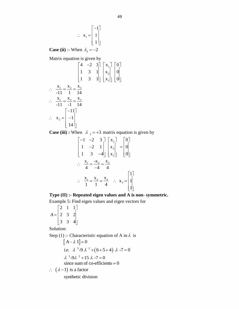
49

1

1

x 1

1

Case (ii) :- When 2 2

Matrix equation is given by

1

2

3

4 2 3 x 0

1 3 1 x 0

1 3 1 x 0

31 2xx x

-11 1 14

31 2xx x

-11 -1 14

2

11

x 1

14

Case (iii) : When 3 3 matrix equation is given by

1

2

3

1 2 3 x 0

1 2 1 x 0

1 3 4 x 0

31 2xx -x

4 4 4

31 23

1xx x

x 11 1 4

1

Type (II) :- Repeated eigen values and A is non- symmetric.

Example 5: Find eigen values and eigen vectors for

2 1 1

2 3 2

3 3 4

A

Solution:

Step (1) :- Characteristic equation of A in is

I 0A

3 2. . -9 6 5 4 -7 0i e

3 2 -9 15 -7 0

since sum of co-efficients 0

1 is a factor

synthetic division

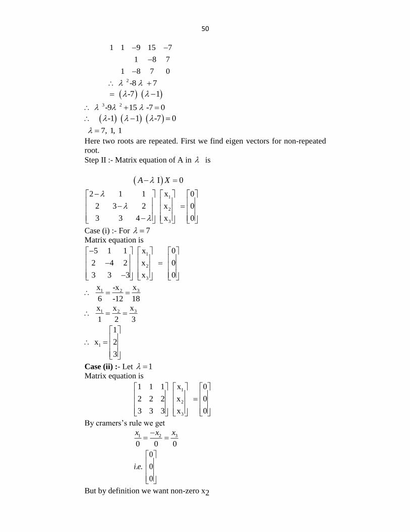
50

1 1 9 15 7

1 8 7

1 8 7 0

2 -8 7

-7 1

3 2 -9 15 -7 0

-1 1 -7 0

7, 1, 1

Here two roots are repeated. First we find eigen vectors for non-repeated

root.

Step II :- Matrix equation of A in is

I 0A X

1

2

3

2 1 1 x 0

2 3 2 x 0

3 3 4 x 0

Case (i) :- For 7

Matrix equation is

1

2

3

5 1 1 x 0

2 4 2 x 0

3 3 3 x 0

31 2xx -x

6 -12 18

31 2xx x

1 2 3

1

1

x 2

3

Case (ii) :- Let 1

Matrix equation is

1

2

3

1 1 1 x 0

2 2 2 x 0

3 3 3 x 0

By cramers‟s rule we get

31 2

0 0 0

xx x

0

. . 0

0

i e

But by definition we want non-zero x2

51

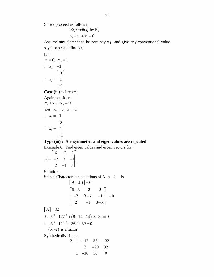
So we proceed as follows

1 by RExpanding

1 2 3 0x x x

Assume any element to be zero say x1 and give any conventional value

say 1 to x2 and find x3

Let

1 20, x 1x

3 1x

2

0

1

1

x

Case (iii) :- Let x=1

Again consider

1 2 3x x x 0

2 1 0, x 1Let x

3 1x

2

0

1

1

x

Type (iii) :- A is symmetric and eigen values are repeated

Example 6: Find eigen values and eigen vectors for .

6 2 2

2 3 1

2 1 3

A

Solution:

Step :- Characteristic equations of A in is

0A I

6 2 2

2 3 1 0

2 1 3

A 32

3 2. . 12 8 14 14 -32 0i e

3 2 12 36 -32 0

-2 is a factor

Synthetic division :-

2 1 12 36 32

2 20 32

1 10 16 0

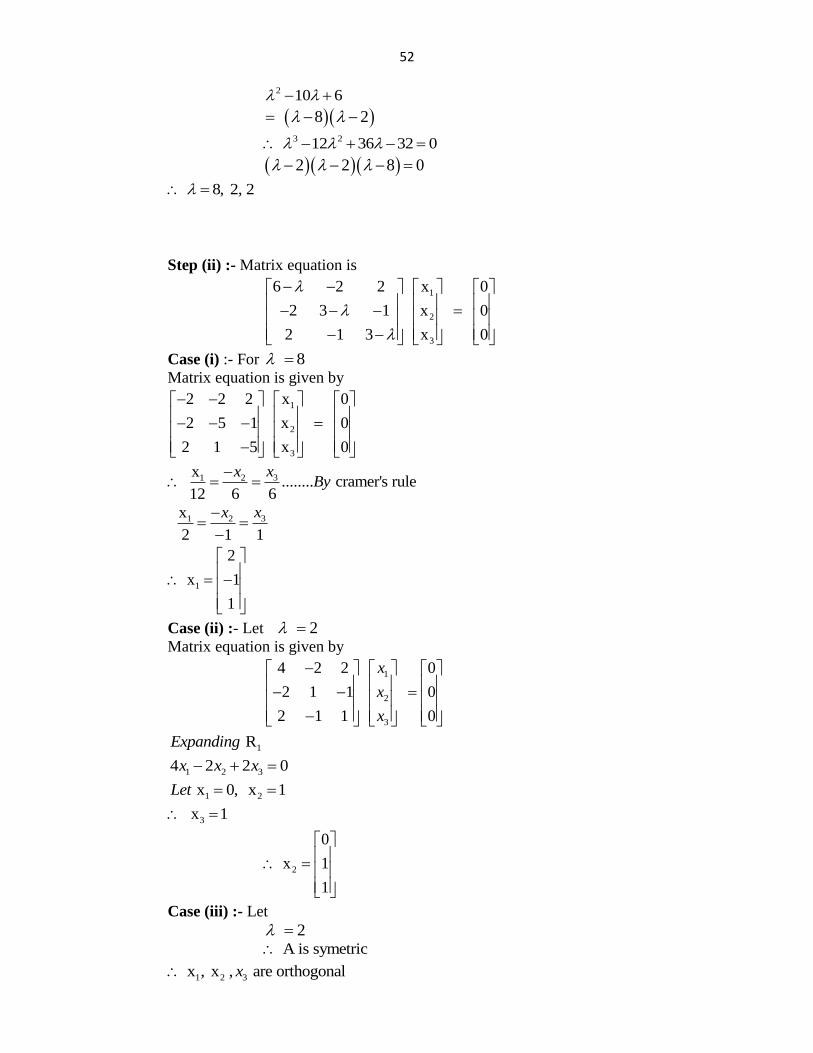
52

2 10 6

8 2

3 2 12 36 32 0

2 2 8 0

8, 2, 2

Step (ii) :- Matrix equation is

1

2

3

6 2 2 x 0

2 3 1 x 0

2 1 3 x 0

Case (i) :- For 8


1

2

3

2 2 2 x 0

2 5 1 x 0

2 1 5 x 0

31 2x ........ cramer's rule 12 6 6

xxBy

31 2x

2 1 1

xx

1

2

x 1

1

Case (ii) :- Let 2


1

2

3

4 2 2 0

2 1 1 0

2 1 1 0

x

x

x

1 RExpanding

1 2 34 2 2 0x x x

1 2 x 0, x 1Let

3 x 1

2

0

x 1

1

Case (iii) :- Let

2 A is symetric

1 2 3 x , x , are orthogonalx

53

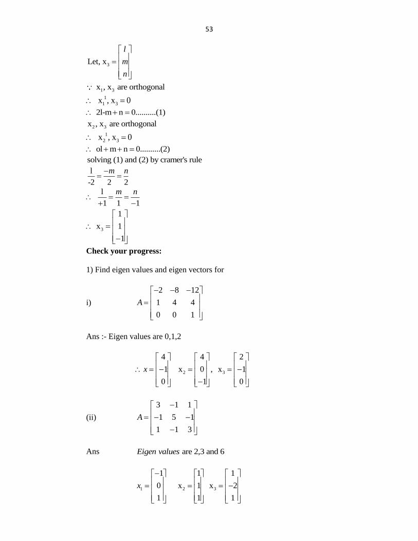
3Let, x

l

m

n

1 3 x , x are orthogonal

1

1 3 x , x 0

2l-m n 0..........(1)

2 3x , x are orthogonal

1

2 3 x , x 0

ol m n 0..........(2)

solving (1) and (2) by cramer's rule

l

-2 2 2

m n

l

1 1 1

m n

3

1

x 1

1


1) Find eigen values and eigen vectors for

i)

2 8 12

1 4 4

0 0 1

A

Ans :- Eigen values are 0,1,2

2 3

4 4 2

1 x 0 , x 1

0 1 0

x

(ii)

3 1 1

1 5 1

1 1 3

A

Ans are 2,3 and 6Eigen values

1 2 3

1 1 1

0 x 1 x 2

1 1 1

x

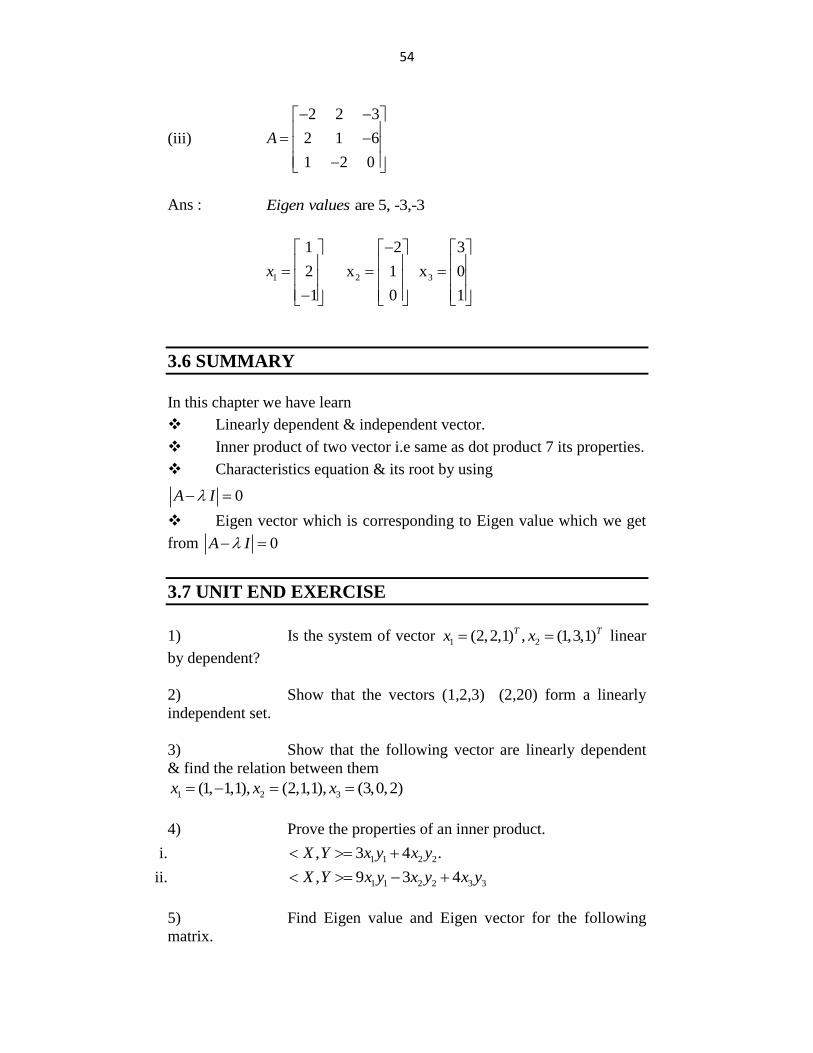
54

(iii)

2 2 3

2 1 6

1 2 0

A

Ans : are 5, -3,-3Eigen values

1 2 3

1 2 3

2 x 1 x 0

1 0 1

x

3.6 SUMMARY


Linearly dependent & independent vector.

Inner product of two vector i.e same as dot product 7 its properties.

Characteristics equation & its root by using

0A I

Eigen vector which is corresponding to Eigen value which we get

from 0A I


1) Is the system of vector 1 2(2,2,1) , (1,3,1)T Tx x linear

by dependent?

2) Show that the vectors (1,2,3) (2,20) form a linearly

independent set.

3) Show that the following vector are linearly dependent

& find the relation between them

1 2 3(1, 1,1), (2,1,1), (3,0,2)x x x

4) Prove the properties of an inner product.

i. 1 1 2 2, 3 4 .X Y x y x y

ii. 1 1 2 2 3 3, 9 3 4X Y x y x y x y

5) Find Eigen value and Eigen vector for the following

matrix.

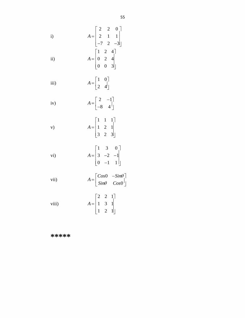
55

i)

2 2 0

2 1 1

7 2 3

A

ii)

1 2 4

0 2 4

0 0 3

A

iii) 1 0

2 4A

iv) 2 1

8 4A

v)

1 1 1

1 2 1

3 2 3

A

vi)

1 3 0

3 2 1

0 1 1

A

vii) 0

0

Cos SinA

Sin Cos

viii)

2 2 1

1 3 1

1 2 1

A

*****

56

4 CAYLEY – HAMILTON THEORY

UNIT STRUCTURE

4.1 Objective

4.2 Introduction

4.3 Cayley – Hamilton Theorem

4.4 Similarity of Matrix

4.5 Characteristics Polynomial

4.6 Minimal Polynomial

4.7 Complex Matrices

4.8 Let Us Sum Up


4.1 OBJECTIVE


Find by using Cayley Hamilton Theorem.

Application of Cayley- Hamilton Theorem.

Find diagonal matrix on similar matrix.

Characteristic Polynomial & Minimal Polynomial of matrix A.

Derogatory & non-derogatory matrix.

Complex matrix like Hermitian, Skew-Hermitian unitary matrix.

4.2 INTRODUCTION

In previous chapter we learn about Eigen values & Eigen Vector. How

here we are going to discuss Cayley Hamilton Theory & its application

also we had study only Real matrix. We introduce here complex matrix

with type of complex matrix also minimal polynomial.

4.3 CAYLEY – HAMILTON THEOREM

Statement: Every square matrix satisfies its own characteristic equation.

If the characteristic Equation for the nth

order square matrix A is

1 2

1 21 ........n n n n

nA I a a a then

1 2

1 21 ........ 0n n n n

nA a A a A a I

57

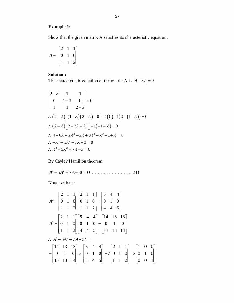
Example 1:

Show that the given matrix A satisfies its characteristic equation.

2 1 1

0 1 0

1 1 2

A

Solution:

The characteristic equation of the matrix A is 0A I

2 1 1

0 1 0 0

1 1 2

2 1 2 0 1 0 1 0 1 0

22 2 3 1 1 0

2 2 34 6 2 2 3 1 0 3 25 7 3 0

3 25 7 3 0

By Cayley Hamilton theorem,

3 25 7 3 0A A A I ………………………..(1)

Now, we have

2

2 1 1 2 1 1 5 4 4

0 1 0 0 1 0 0 1 0

1 1 2 1 1 2 4 4 5

A

3

2 1 1 5 4 4 14 13 13

0 1 0 0 1 0 0 1 0

1 1 2 4 4 5 13 13 14

A

3 25 7 3A A A I

14 13 13 5 4 4 2 1 1 1 0 0

0 1 0 -5 0 1 0 +7 0 1 0 3 0 1 0

13 13 14 4 4 5 1 1 2 0 0 1

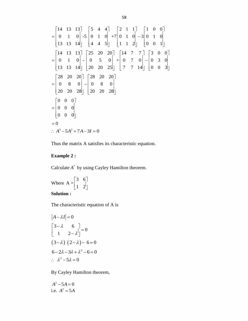
58

14 13 13 5 4 4 2 1 1 1 0 0

0 1 0 -5 0 1 0 +7 0 1 0 3 0 1 0

13 13 14 4 4 5 1 1 2 0 0 1

14 13 13 25 20 20 14 7 7 3 0 0

0 1 0 - 0 5 0 + 0 7 0 0 3 0

13 13 14 20 20 25 7 7 14 0 0 3

28 20 20 28 20 20

0 8 0 0 8 0

20 20 28 20 20 28

0 0 0

0 0 0

0 0 0

0 3 25 7 3 0A A A I

Thus the matrix A satisfies its characteristic equation.

Example 2 :

Calculate 7A by using Cayley Hamilton theorem.

Where

3 6A =

1 2

Solution :

The characteristic equation of A is

0A I

3 60

1 2

3 2 6 0

26 2 3 6 0 2 5 0

By Cayley Hamilton theorem,

2 5 0A A

i.e. 2 5A A

59

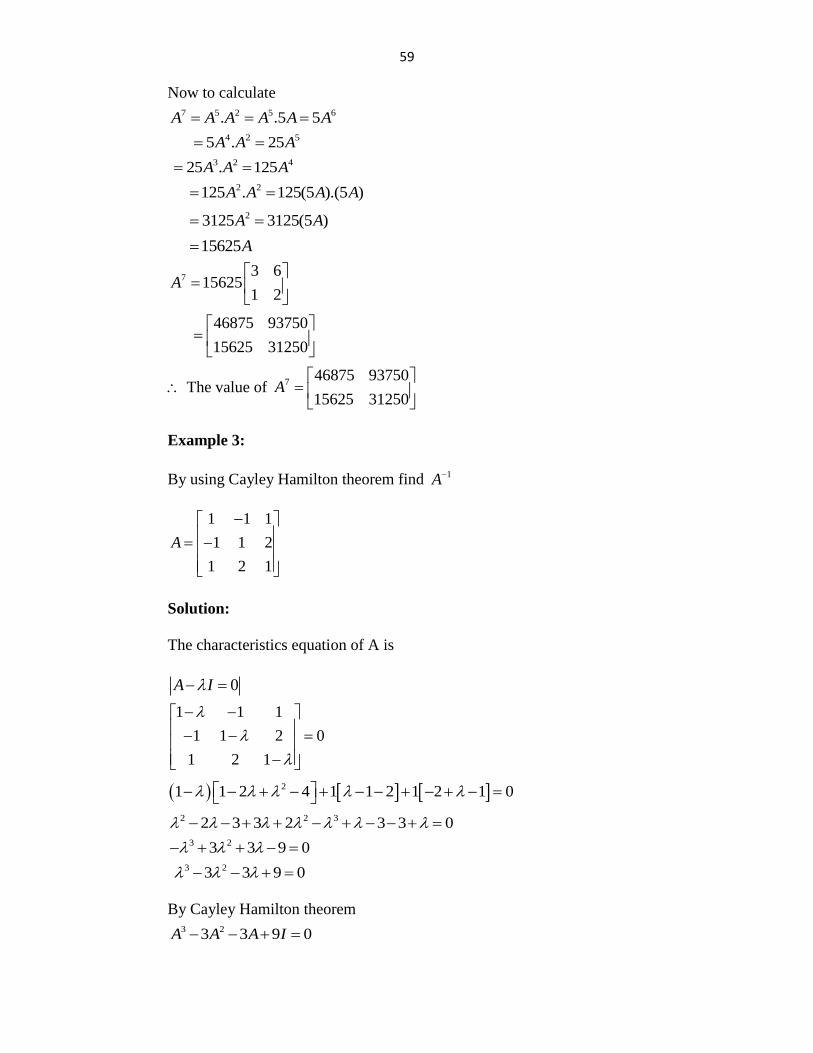
Now to calculate 7 5 2 5 6. .5 5A A A A A A

4 2 55 . 25A A A

3 2 425 . 125A A A

2 2125 . 125(5 ).(5 )A A A A

23125 3125(5 )A A

15625A

73 6

156251 2

A

46875 93750

15625 31250

The value of 7

46875 93750

15625 31250A

Example 3:

By using Cayley Hamilton theorem find 1A

1 1 1

1 1 2

1 2 1

A

Solution:

The characteristics equation of A is

0A I

1 1 1

1 1 2 0

1 2 1

21 1 2 4 1 1 2 1 2 1 0

2 2 32 3 3 2 3 3 0 3 23 3 9 0

3 2 3 3 9 0

By Cayley Hamilton theorem 3 23 3 9 0A A A I

60

Multiply by 1A

3 1 2 1 1 1 1 3 3 9 0A A A A AA IA A

2 1 3 3 9 0A A I A

1 21 3 3

9A A I A …….(1)

2

1 1 1 1 1 1 3 0 0

1 1 2 1 1 2 0 6 3

1 2 1 1 2 1 0 3 6

A

1 1 1 1 0 0 3 0 0

3 3 3 1 1 2 3 0 1 0 0 6 3

1 2 1 0 0 1 0 3 6

A I A

2

3 3 3 3 0 0 3 0 0

3 3 3 3 6 0 3 0 0 6 3

3 6 3 0 0 3 0 3 6

A I A

3 3 3

3 0 3

3 3 0

1 213 3

9A A I A

3 3 31

3 0 39

3 3 0

1 1 11

1 0 13

1 1 0

1

1 1 11

1 0 13

1 1 0

A


1) Find the characteristic polynomial of the matrix.

3 1 1

1 5 1

1 1 3

A

Verify Cayley-Hamilton theorem for this matrix.

61

Hence find 1A

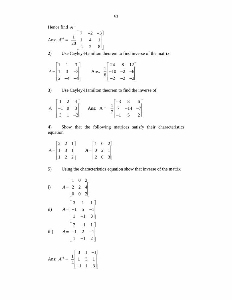
Ans: 1

7 2 31

1 4 120

2 2 8

A

2) Use Cayley-Hamilton theorem to find inverse of the matrix.

1 1 3

1 3 3

2 4 4

A

Ans:

24 8 121

10 2 68

2 2 2

3) Use Cayley-Hamilton theorem to find the inverse of

1 2 4

1 0 3

3 1 2

A

Ans: 1

3 8 61

A 7 14 77

1 5 2

4) Show that the following matrices satisfy their characteristics

equation

2 2 1

1 3 1

1 2 2

A

1 0 2

0 2 1

2 0 3

A

5) Using the characteristics equation show that inverse of the matrix

i)

1 0 2

2 2 4

0 0 2

A

ii)

3 1 1

1 5 1

1 1 3

A

iii)

2 1 1

1 2 1

1 1 2

A

Ans: 1

3 1 11

1 3 14

1 1 3

A

62

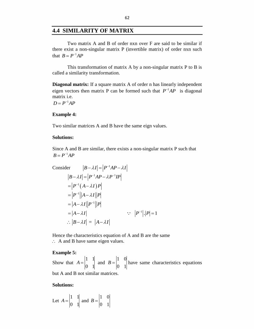
4.4 SIMILARITY OF MATRIX

Two matrix A and B of order nxn over F are said to be similar if

there exist a non-singular matrix P (invertible matrix) of order nxn such

that 1B P AP

This transformation of matrix A by a non-singular matrix P to B is

called a similarity transformation.

Diagonal matrix: If a square matrix A of order n has linearly independent

eigen vectors then matrix P can be formed such that 1P AP is diagonal

matrix i.e. 1D P AP

Example 4:

Two similar matrices A and B have the same eign values.

Solutions:

Since A and B are similar, there exists a non-singular matrix P such that 1B P AP

Consider 1B I P AP I

1 1B I P AP P IP

1P A I P

1P A I P

1A I P P

1 . 1A I P P

= B I A I

Hence the characteristics equation of A and B are the same

A and B have same eigen values.

Example 5:

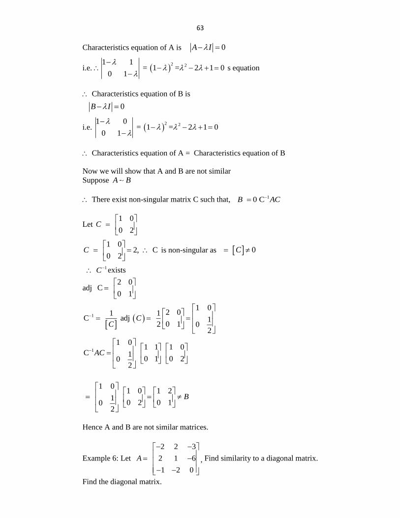
Show that 1 1

0 1A and

1 0

0 1B have same characteristics equations

but A and B not similar matrices.

Solutions:

Let 1 1

0 1A and

1 0

0 1B

63

Characteristics equation of A is 0A I

i.e. 2 2

1 1 = 1 = 2 1 0

0 1

s equation

Characteristics equation of B is

0B I

i.e. 2 2

1 0 = 1 = 2 1 0

0 1

Characteristics equation of A = Characteristics equation of B

Now we will show that A and B are not similar

Suppose A B

There exist non-singular matrix C such that, 1 0 CB AC

Let 1 0

0 2

C

1 0 2, C

0 2C

is non-singular as 0C

1 C exists

adj 2 0

C 0 1

1

1 02 01 1

C adj 10 12 0

2

CC

1

1 01 1 1 0

C 10 1 0 20

2

AC

1 01 0 1 2

10 2 0 10

2

B

Hence A and B are not similar matrices.

Example 6: Let

2 2 3

2 1 6

1 2 0

A

, Find similarity to a diagonal matrix.

Find the diagonal matrix.

64

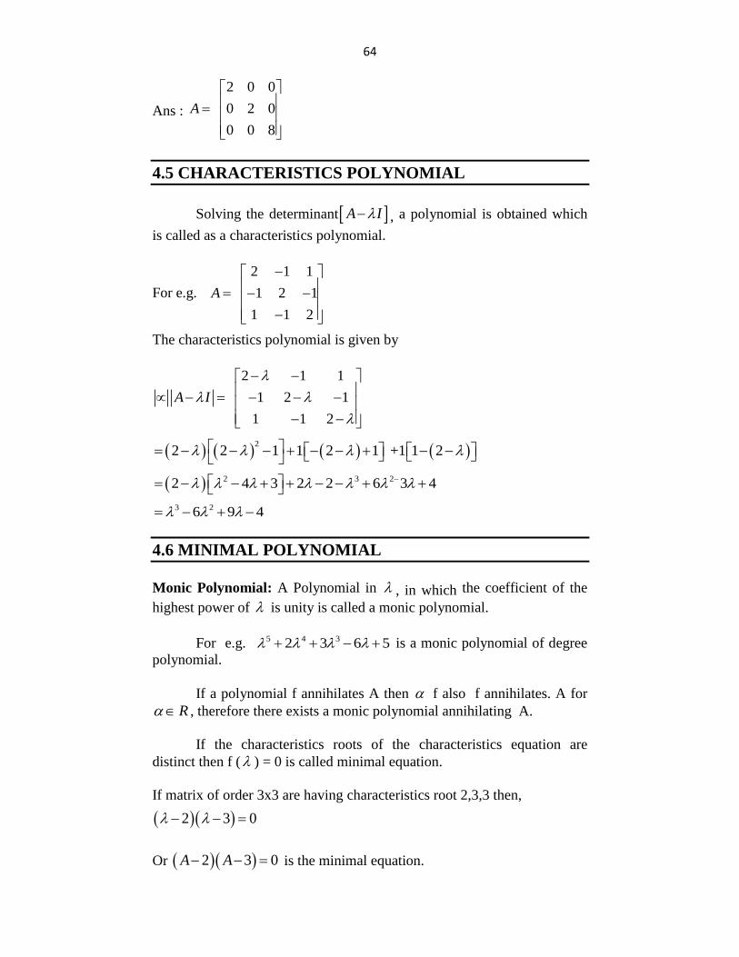
Ans :

2 0 0

0 2 0

0 0 8

A

4.5 CHARACTERISTICS POLYNOMIAL

Solving the determinant A I , a polynomial is obtained which

is called as a characteristics polynomial.

For e.g.

2 1 1

1 2 1

1 1 2

A

The characteristics polynomial is given by

2 1 1

1 2 1

1 1 2

A I

2

2 2 1 1 2 1 +1 1 2

2 3 22 4 3 2 2 6 3 4

3 26 9 4

4.6 MINIMAL POLYNOMIAL

Monic Polynomial: A Polynomial in , in which the coefficient of the

highest power of is unity is called a monic polynomial.

For e.g. 5 4 32 3 6 5 is a monic polynomial of degree

polynomial.

If a polynomial f annihilates A then f also f annihilates. A for

R , therefore there exists a monic polynomial annihilating A.

If the characteristics roots of the characteristics equation are

distinct then f ( ) = 0 is called minimal equation.

If matrix of order 3x3 are having characteristics root 2,3,3 then,

2 3 0

Or 2 3 0A A is the minimal equation.

65

Hence the degree of the equation is 2 and less than the order of the

polynomial.

Derogatory Matrix: A nxn matrix is called derogatory if the degree of its

minimal polynomial is less than n.

Non-Derogatory Matrix: A nxn matrix is called non-derogatory if the

degree of minimal polynomial is equal to n.

Properties of Minimal Polynomial:

(1) There exists a unique minimal polynomial of the matrix A.

(2) The minimal polynomial of A divides the characteristics

polynomial of A.

(3) If is the root of the minimal polynomial of A then is also

characteristics of root of A.

(4) If the n characteristics of root of A are distinct then A is non

derogatory.

Example 7:

Check whether the following matrix is derogatory or non derogatory also

find its minimal polynomial.

i)

2 2 3

1 1 1

1 3 1

A

Solution:

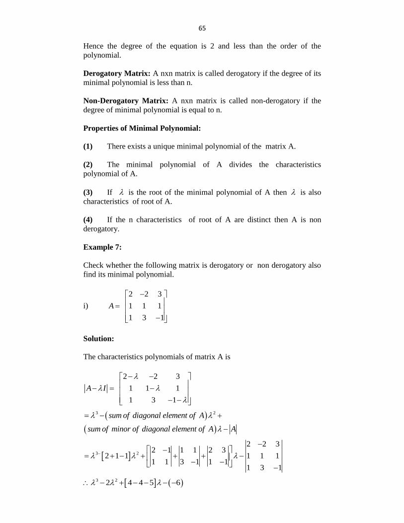
The characteristics polynomials of matrix A is

2 2 3

1 1 1

1 3 1

A I

3 2sum of diagonal element of A

sum of minor of diagonal element of A A

3 2

2 2 32 1 1 1 2 3

2 1 1 1 1 11 1 3 1 1 1

1 3 1

3 22 4 4 5 6

66

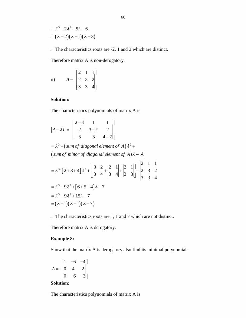
3 22 5 6

2 1 3

The characteristics roots are -2, 1 and 3 which are distinct.

Therefore matrix A is non-derogatory.

ii)

2 1 1

2 3 2

3 3 4

A

Solution:


2 1 1

2 3 2

3 3 4

A I


sum of minor of diagonal element of A A

3 2

2 1 13 2 2 1 2 1

2 3 4 2 3 23 4 3 4 2 3

3 3 4

3 29 6 5 4 7

3 29 15 7

1 1 7

The characteristics roots are 1, 1 and 7 which are not distinct.

Therefore matrix A is derogatory.

Example 8:

Show that the matrix A is derogatory also find its minimal polynomial.

1 6 4

0 4 2

0 6 3

A

Solution:


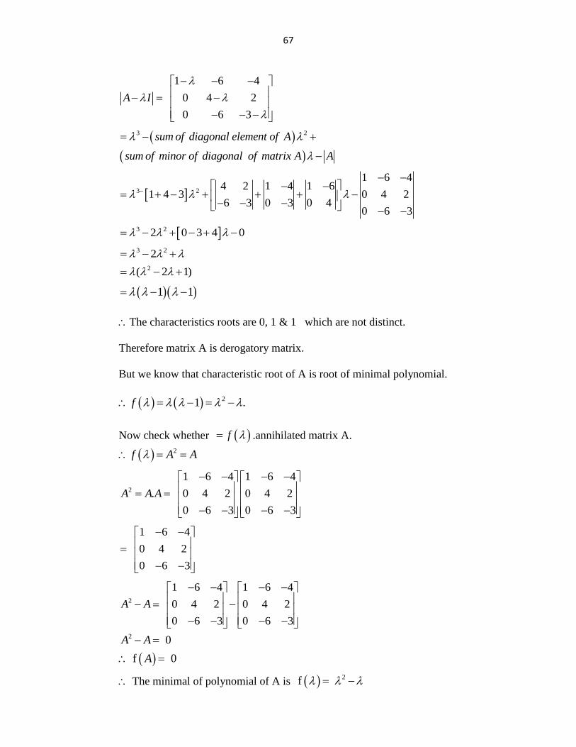
67

1 6 4

0 4 2

0 6 3

A I


sum of minor of diagonal of matrix A A

3 2

1 6 44 2 1 4 1 6

1 4 3 0 4 26 3 0 3 0 4

0 6 3

3 22 0 3 4 0

3 22 2( 2 1)

1 1

The characteristics roots are 0, 1 & 1 which are not distinct.

Therefore matrix A is derogatory matrix.

But we know that characteristic root of A is root of minimal polynomial.

21 .f

Now check whether f .annihilated matrix A.

2f A A

2

1 6 4 1 6 4

. 0 4 2 0 4 2

0 6 3 0 6 3

A A A

1 6 4

0 4 2

0 6 3

2

1 6 4 1 6 4

0 4 2 0 4 2

0 6 3 0 6 3

A A

2 0A A

f 0A

The minimal of polynomial of A is 2f

68

& degree of polynomial is 2 which is less than 3

Hence matrix A is derogatory.

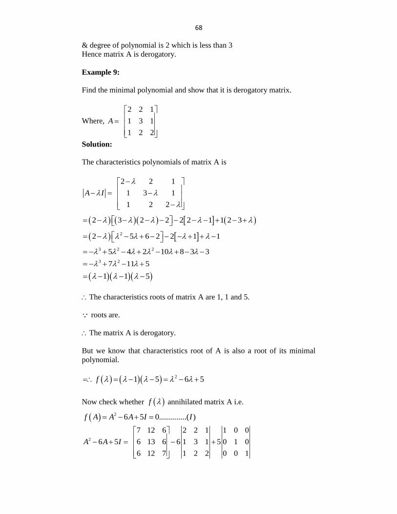
Example 9:

Find the minimal polynomial and show that it is derogatory matrix.

Where,

2 2 1

1 3 1

1 2 2

A

Solution:


2 2 1

1 3 1

1 2 2

A I

2 3 2 2 2 2 1 1 2 3

22 5 6 2 2 1 1 3 2 25 4 2 10 8 3 3

3 27 11 5

1 1 5

The characteristics roots of matrix A are 1, 1 and 5.

roots are.

The matrix A is derogatory.

But we know that characteristics root of A is also a root of its minimal

polynomial.

21 5 6 5f

Now check whether f annihilated matrix A i.e.

2 6 5 0..............( )f A A A I I

2

7 12 6 2 2 1 1 0 0

6 5 6 13 6 6 1 3 1 5 0 1 0

6 12 7 1 2 2 0 0 1

A A I

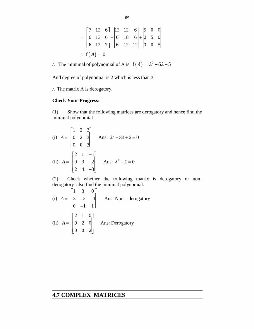
69

7 12 6 12 12 6 5 0 0

6 13 6 6 18 6 0 5 0

6 12 7 6 12 12 0 0 5

f 0A

The minimal of polynomial of A is 2f 6 5

And degree of polynomial is 2 which is less than 3

The matrix A is derogatory.


(1) Show that the following matrices are derogatory and hence find the

minimal polynomial.

(i)

1 2 3

0 2 3

0 0 3

A

Ans: 2 3 2 0

(ii)

2 1 1

0 3 2

2 4 3

A

Ans: 2 0

(2) Check whether the following matrix is derogatory or non-

derogatory also find the minimal polynomial.

(i)

1 3 0

3 2 1

0 1 1

A

Ans: Non – derogatory

(ii)

2 1 0

0 2 0

0 0 2

A

Ans: Derogatory

4.7 COMPLEX MATRICES

70

Z =x+iy is called a complex number, where 1i and ,x y R and

Z x iy

is called a conjugate of the complex number Z

Let A be a mxn matrix having complex numbers as its elements, then the

matrix is called a complex matrix.

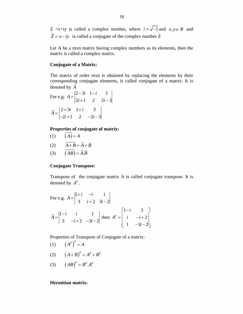
Conjugate of a Matrix:

The matrix of order mxn is obtained by replacing the elements by their

corresponding conjugate elements, is called conjugate of a matrix. It is

denoted by A

For e.g. 2 3 1 3

2 1 2 2 3

i iA

i i

2 3 1 3

2 1 2 2 3

i iA

i i

Properties of conjugate of matrix:

(1) A A

(2) A B A B

(3) .AB A B

Conjugate Transpose:

Transpose of the conjugate matrix A is called conjugate transpose. It is

denoted by A .

For e.g. 1 1

3 2 3 2

i iA

i i

1 1

3 2 3 2

i iA

i i

then

1 3

2

1 3 2

i

A i i

i

Properties of Transpose of Conjugate of a matrix:

(1) A A

(2) A B A B

(3) .AB B A

Hermitian matrix:

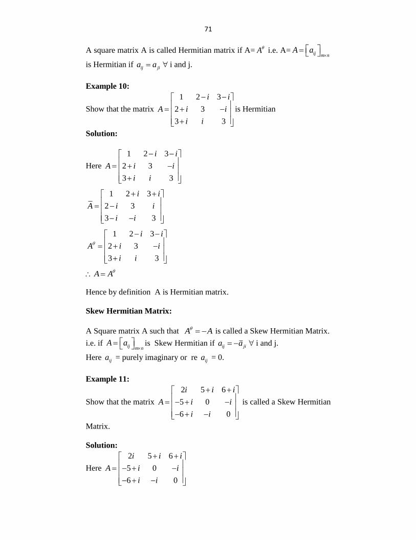
71

A square matrix A is called Hermitian matrix if A= A i.e. A= ij m nA a

is Hermitian if ij jia a i and j.

Example 10:

Show that the matrix

1 2 3

2 3

3 3

i i

A i i

i i

is Hermitian

Solution:

Here

1 2 3

2 3

3 3

i i

A i i

i i

1 2 3

2 3

3 3

i i

A i i

i i

1 2 3

2 3

3 3

i i

A i i

i i

A A

Hence by definition A is Hermitian matrix.

Skew Hermitian Matrix:

A Square matrix A such that A A is called a Skew Hermitian Matrix.

i.e. if ij m nA a

is Skew Hermitian if ij jia a i and j.

Here ija = purely imaginary or

re ija = 0.

Example 11:

Show that the matrix

2 5 6

5 0

6 0

i i i

A i i

i i

is called a Skew Hermitian

Matrix.

Solution:

Here

2 5 6

5 0

6 0

i i i

A i i

i i

72

2 5 6

5 0

6 0

i i i

A i i

i i

2 5 6

5 0

6 0

i i i

A i i

i i

2 5 6

5 0

6 0

i i i

A i i

i i

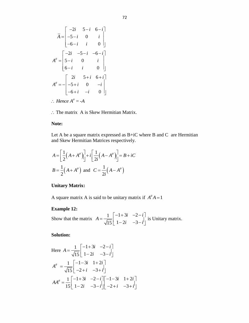
θHence A = -A

The matrix A is Skew Hermitian Matrix.

Note:

Let A be a square matrix expressed as B+iC where B and C are Hermitian

and Skew Hermitian Matrices respectively.

1 1

2 2A A A i A A B iC

i

1

2B A A and

1

2C A A

i

Unitary Matrix:

A square matrix A is said to be unitary matrix if 1A A

Example 12:

Show that the matrix 1 3 21

1 2 315

i iA

i i

is Unitary matrix.

Solution:

Here 1 3 21

1 2 315

i iA

i i

1 3 1 21

2 315

i iA

i i

1 3 2 1 3 1 21

1 2 3 2 315

i i i iAA

i i i i

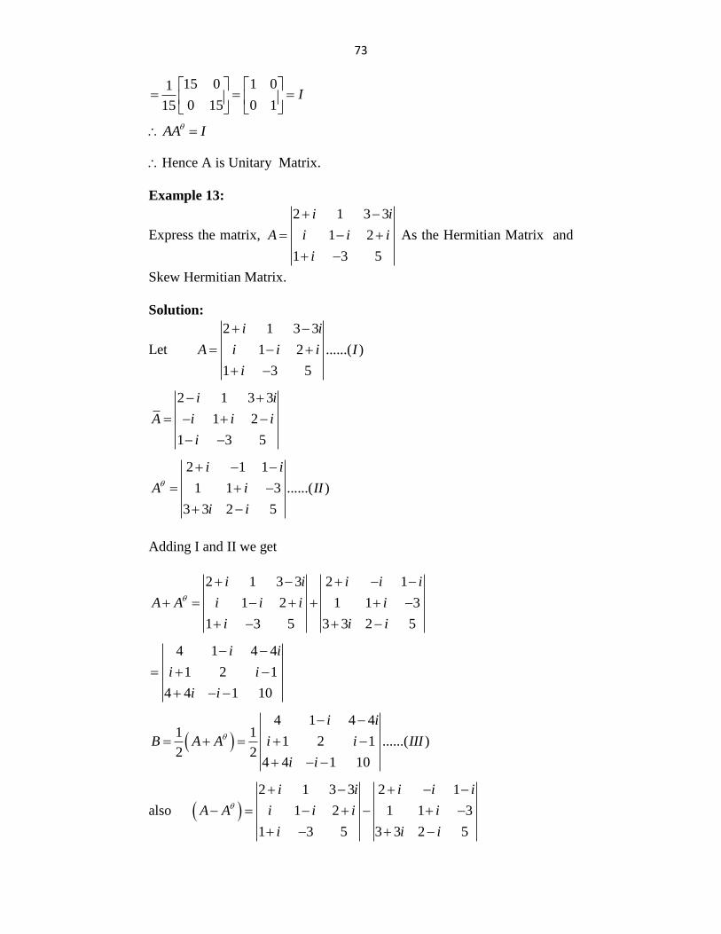
73

15 0 1 01

0 15 0 115I

AA I

Hence A is Unitary Matrix.

Example 13:

Express the matrix,

2 1 3 3

1 2

1 3 5

i i

A i i i

i

As the Hermitian Matrix and

Skew Hermitian Matrix.

Solution:

Let

2 1 3 3

1 2 ......( )

1 3 5

i i

A i i i I

i

2 1 3 3

1 2

1 3 5

i i

A i i i

i

2 1 1

1 1 3 ......( )

3 3 2 5

i i

A i II

i i

Adding I and II we get

2 1 3 3 2 1

1 2 1 1 3

1 3 5 3 3 2 5

i i i i i

A A i i i i

i i i

4 1 4 4

1 2 1

4 4 1 10

i i

i i

i i

4 1 4 4

1 11 2 1 ......( )

2 24 4 1 10

i i

B A A i i III

i i

also 2 1 3 3 2 1

1 2 1 1 3

1 3 5 3 3 2 5

i i i i i

A A i i i i

i i i

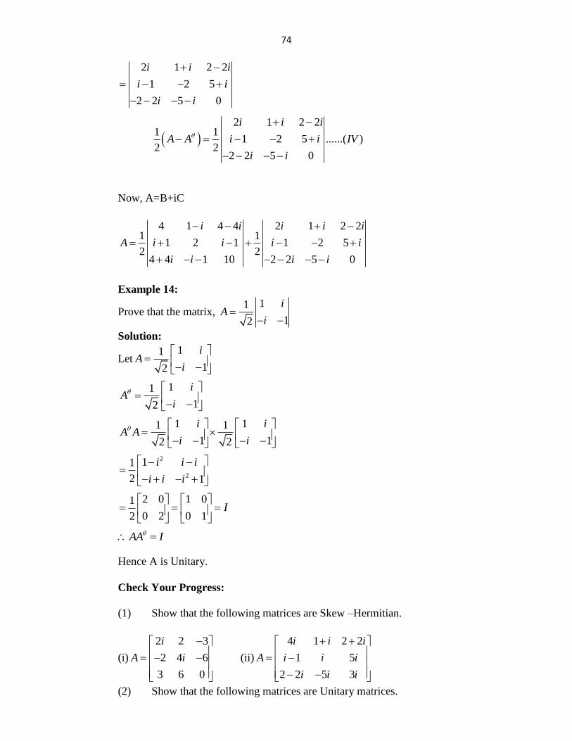
74

2 1 2 2

1 2 5

2 2 5 0

i i i

i i

i i

2 1 2 2

1 11 2 5 ......( )

2 22 2 5 0

i i i

A A i i IV

i i

Now, A=B+iC

4 1 4 4 2 1 2 21 1

1 2 1 1 2 52 2

4 4 1 10 2 2 5 0

i i i i i

A i i i i

i i i i

Example 14:

Prove that the matrix, 11

12

iA

i

Solution:

Let11

12

iA

i

11

12

iA

i

1 11 1

1 12 2

i iA A

i i

2

2

11

2 1

i i i

i i i

2 0 1 01

0 2 0 12I

AA I

Hence A is Unitary.


(1) Show that the following matrices are Skew –Hermitian.

(i)

2 2 3

2 4 6

3 6 0

i

A i

(ii)

4 1 2 2

1 5

2 2 5 3

i i i

A i i i

i i i

(2) Show that the following matrices are Unitary matrices.

75

(i)1 11

1 13

iA

i

(ii)

1 11

1 12

i iA

i i

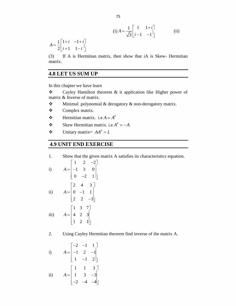
(3) If A is Hermitian matrix, then show that iA is Skew- Hermitian

matrix.

4.8 LET US SUM UP


Cayley Hamilton theorem & it application like Higher power of

matrix & Inverse of matrix.

Minimal .polynomial & derogatory & non-derogatory matrix.

Complex matrix.

Hermitian matrix. i.e A A

Skew Hermitian matrix. i.e A A

Unitary matrix= .AA I


1. Show that the given matrix A satisfies its characteristics equation.

i)

1 2 2

1 3 0

0 2 1

A

ii)

2 4 3

0 1 1

2 2 1

A

iii)

1 3 7

4 2 3

1 2 1

A

2. Using Cayley Hermitian theorem find inverse of the matrix A.

i)

2 1 1

1 2 1

1 1 2

A

ii)

1 1 3

1 3 3

2 4 4

A

76

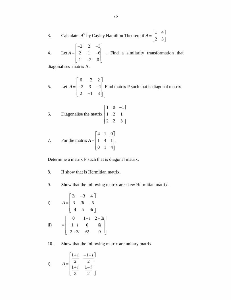
3. Calculate 5A by Cayley Hamilton Theorem if1 4

2 3A

4. Let

2 2 3

2 1 6

1 2 0

A

. Find a similarity transformation that

diagonalises matrix A.

5. Let

6 2 2

2 3 1

2 1 3

A

.

Find matrix P such that is diagonal matrix

6. Diagonalise the matrix

1 0 1

1 2 1

2 2 3

7. For the matrix

4 1 0

1 4 1 .

0 1 4

A

Determine a matrix P such that is diagonal matrix.

8. If show that is Hermitian matrix.

9. Show that the following matrix are skew Hermitian matrix.

i)

2 3 4

3 3 5

4 5 4

i

A i

i

ii)

0 1 2 3

1 0 6

2 3 6 0

i i

i i

i i

10. Show that the following matrix are unitary matrix

i)

1 1

2 2

1 1

2 2

i i

Ai i

77

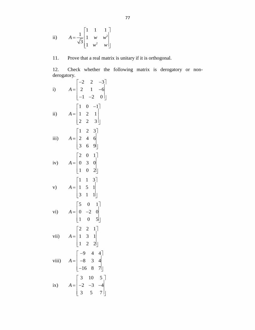
ii) 2

2

1 1 11

13

1

A w w

w w

11. Prove that a real matrix is unitary if it is orthogonal.

12. Check whether the following matrix is derogatory or non-

derogatory.

i)

2 2 3

2 1 6

1 2 0

A

ii)

1 0 1

1 2 1

2 2 3

A

iii)

1 2 3

2 4 6

3 6 9

A

iv)

2 0 1

0 3 0

1 0 2

A

v)

1 1 3

1 5 1

3 1 1

A

vi)

5 0 1

0 2 0

1 0 5

A

vii)

2 2 1

1 3 1

1 2 2

A

viii)

9 4 4

8 3 4

16 8 7

A

ix)

3 10 5

2 3 4

3 5 7

A

78

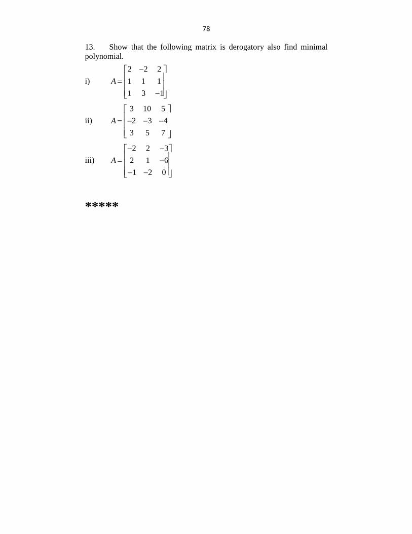
13. Show that the following matrix is derogatory also find minimal

polynomial.

i)

2 2 2

1 1 1

1 3 1

A

ii)

3 10 5

2 3 4

3 5 7

A

iii)

2 2 3

2 1 6

1 2 0

A

*****

79

5 VECTOR CALCULAS

UNIT STRUCTURE

5.0 Objectives

5.1 Introduction

5.2 Vector differentiation

5.3 Vector operator

5.3.1 Gradient

5.3.2 Geometric meaning of gradient

5.3.3 Divergence

5.3.4 Solenoidal function

5.3.5 Curl

5.3.6 Irrational field

5.4 Properties of gradient, divergence and curl

5.5 Let Us Sum Up


5.0 OBJECTIVES

After going through this unit, you will be able to

Learn vector differentiation.

Operators, del, grad and curl.

Properties of operators

5.1 INTRODUCTION

Vector algebra deals with addition, subtraction and multiplication of

vertex. In vector calculus we shall study differentiation of vectors

functions, gradient, divergence and curl.

Vector:

Vector is a physical quantity which required magnitude and direction both.

Unit Vector:

80

Unit Vector is a vector which has magnitude 1. Unit vectors along co-

ordinate axis are i and ˆ j , k respectively.

ˆˆ ˆ 1 i = j = k =

Scalar Triple Vector:

Scalar triple product of three vectors is defined as a. b c or a b c .

Geometrical meaning of a b c

is volume of parallelepiped with cotter

minus edges a, b and c .

We have,

a b c = b c a = c a b

a b c = - b a c

Vector Triple Product:

Vector triple product of a b and c is cross product of a and b c i.e.

a b c or cross product of a b and c

a b c = a . c b a . b c

a b c = a . c b b . c a

Remark : Vector triple product is not associative in general

i.e. a b c a b c

Coplanar Vectors:

Three vectors a, b and c are coplanar if a b c

= 0 for

a 0 , b 0 , c 0

5.2 VECTORS DIFFERENTIATION

Let v be a vector function of a scalar t. Let v be the small increment in

a corresponding to the increment t in t.

Then,

81

v v t + t - v(t)

v t + t - v(t)v =

t t

Taking limit t 0 we get,

t 0 t 0

t 0 t 0

t 0

v t + t - v(t)vlim = lim

t t

v t + t - v(t)dv v = lim = lim

dt t t

v t + t - v(t)dv = lim

dt t

Formulas of vector differentiation:

(i) d dv

= k v = k k is a constantdt dt

(ii) d du dv

u + v = dt dt dt

(iii) d dv du

u . v = u . v .dt dt dt

(iv) d dv du

u v = u vdt dt dt

(v) If 1 2 3ˆ ˆ ˆv v i + v j + v k

Then,

31 2dvdv dvdv ˆ ˆ ˆ i + j + k

dt dt dt dt

Note:

If

ˆ ˆ ˆr xi + yj + zk then r = r 2 2 2= x y z

Example 1:

If

2 2ˆ ˆ ˆr t + 1 i + t + t - 1 j + t - t + 1 k find dr

dt and

2d r

dt

82

Solution:–

2 2

2

2

ˆ ˆ ˆr t + 1 i + t + t - 1 j + t - t + 1 k

dr ˆ ˆ ˆ i + 2t + 1 j + 2t - 1 kdt

d r ˆ ˆ 2j + 2 kdt

Example 2:

If

r a cos wt + b sin wt where w is constant show that

dr

r = w a bdt

and 2

2

d r = -w r

dt

Solution: –

r a cos wt + b sin wt------------ (i)

dr a cos wt + b sin wt------------ (ii)

dt

dr r a cos wt + b sin wt -aw sin wt + bw cos wt

dt

2 2

2 2

2 2

a a = 0 a b w cos wt b a w sin wt

b b = 0

b a = 0 a b w cos wt a b w sin wt

= -a b

a b w cos wt sin

wt

a b w 1

w a b

Again differentiating eqn (ii) w.r.t. „t‟

22 2

2

2

2

d r -a w cos wt - b w sin wt

dt

= -w a cos wt + b sin wt

-w r from (i)

Example 3. Evaluate the following:

i) d

a b cdt

ii)

2

2

d da d a a

dt dt dt

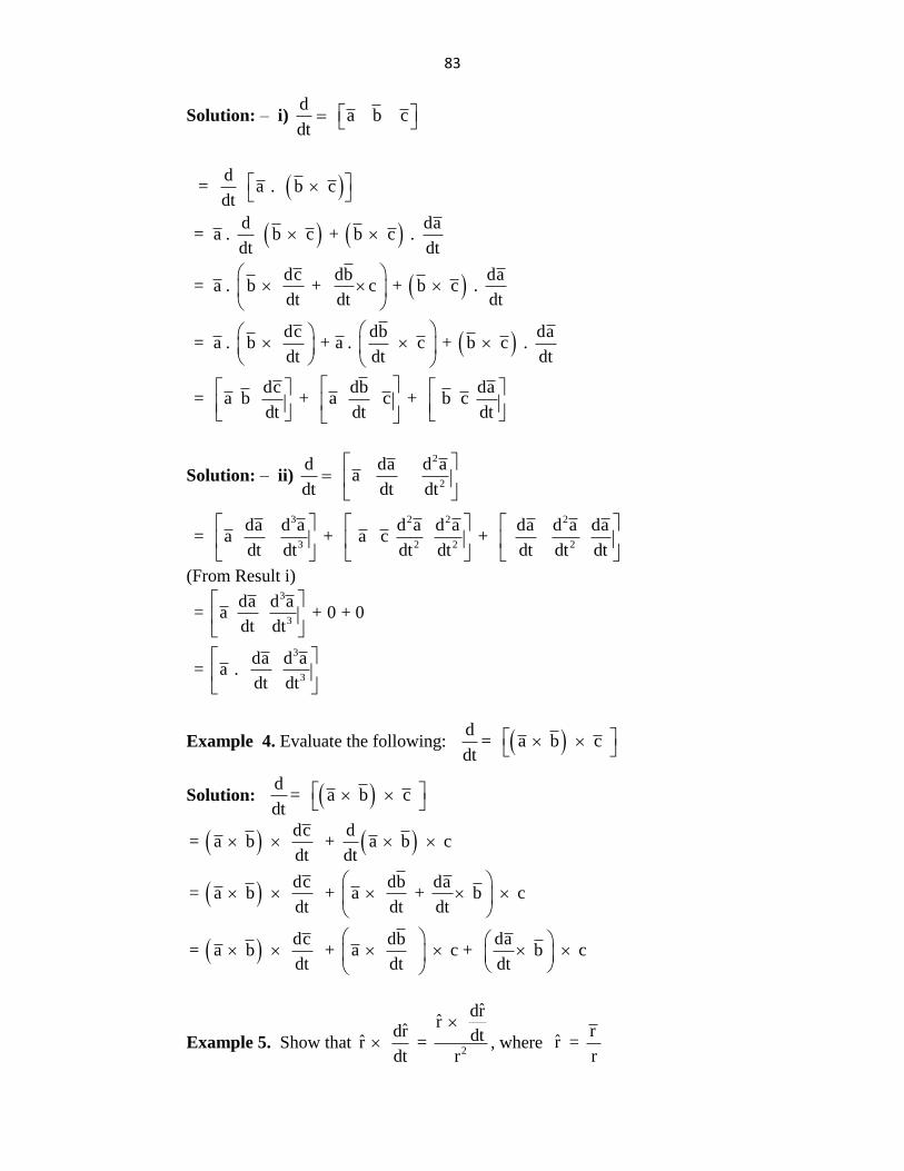
83

Solution: – i) d

a b cdt

d = a . b c

dt

d da = a . b c + b c .

dt dt

dc db da = a . b + c + b c .

dt dt dt

dc db da = a . b + a . c + b c .

dt dt dt

dc db da = a b + a c + b c

dt dt dt

Solution: – ii)

2

2

d da d a a

dt dt dt

3 2 2 2

3 2 2 2

da d a d a d a da d a da = a + a c +

dt dt dt dt dt dt dt

(From Result i)

3

3

3

3

da d a = a + 0 + 0

dt dt

da d a = a .

dt dt

Example 4. Evaluate the following: d

= a b c dt

Solution: d

= a b c dt

dc d= a b + a b c

dt dt

dc db da= a b + a + b c

dt dt dt

dc db da= a b + a c + b c

dt dt dt

Example 5. Show that2

ˆdrr

ˆdr dtˆ r = dt r

, where r

ˆ r = r

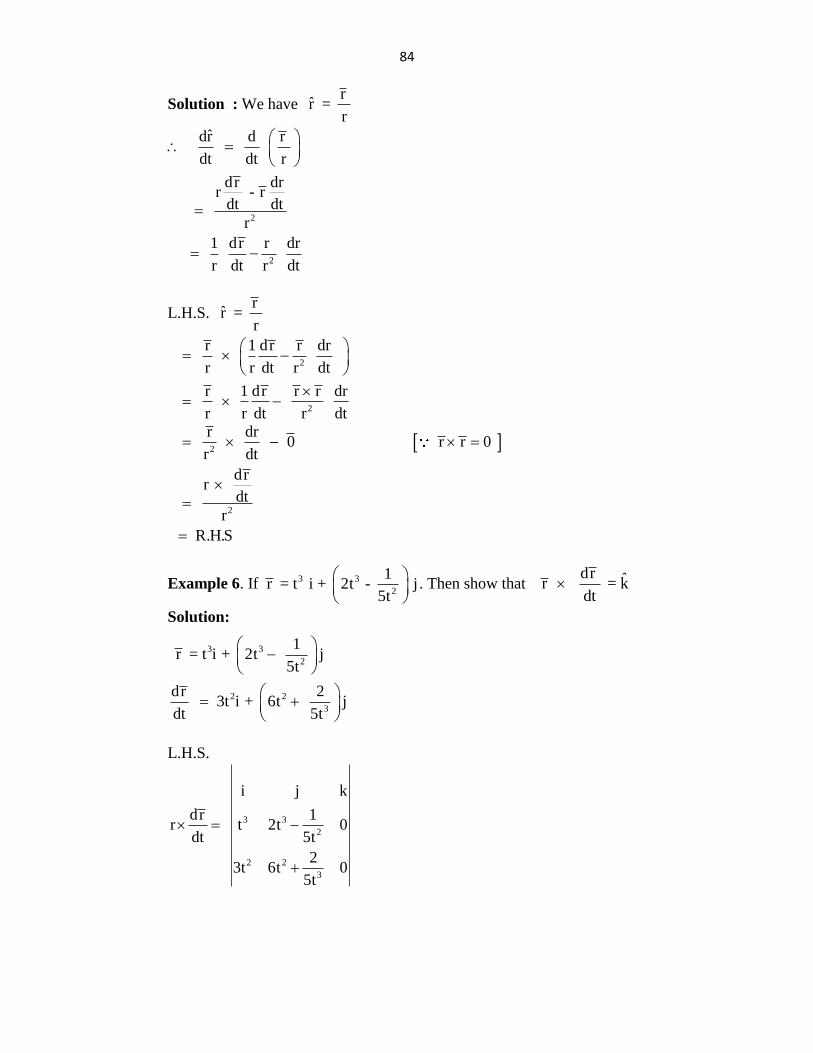
84

Solution : We have

r ˆ r =

r

2

2

ˆdr d r

dt dt r

dr drr - r

dt dt r

1 dr r dr

r dt r dt

L.H.S. r

ˆ r = r

2

2

r 1 dr r dr

r r dt r dt

r 1 dr r r dr

r r dt r dt

2

2

r dr 0 r r 0

r dt

drr

dt r

R.H.S

Example 6. If 3 3

2

1 r = t i + 2t - j

5t

. Then show that dr ˆ r = kdt

Solution:

3 3

2

2 2

3

1 r = t i + 2t j

5t

dr 2 3t i + 6t j

dt 5t

L.H.S.

3 3

2

2 2

3

i j k

dr 1r t 2t 0

dt 5t

23t 6t 0

5t

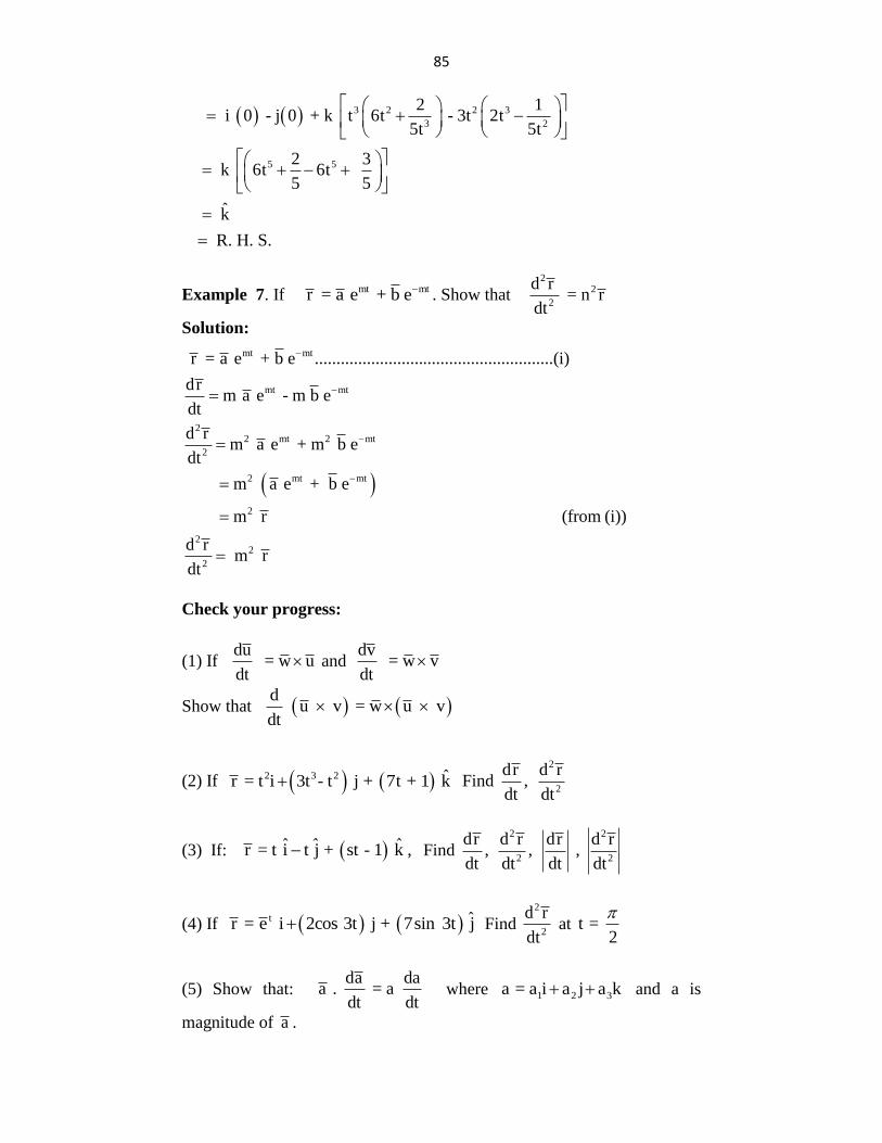
85

3 2 2 3

3 2

5 5

2 1 i 0 - j 0 + k t 6t - 3t 2t

5t 5t

2 3 k 6t 6t

5 5

ˆ k

R. H. S.

Example 7. If mt mt r = a e + b e . Show that

22

2

d r = n r

dt

Solution:

mt mt

mt mt

22 mt 2 mt

2

2 mt mt

2

r = a e + b e .......................................................(i)

drm a e - m b e

dt

d rm a e + m b e

dt

m a e + b e

m r

22

2

(from (i))

d r m r

dt


(1) If du

= w udt

anddv

= w vdt

Show that d

u v = w u vdt

(2) If 2 3 2 ˆ r = t i 3t - t j + 7t + 1 k

Find 2

2

dr d r,

dt dt

(3) If:

ˆ ˆ ˆ r = t i t j + st - 1 k ,

Find 2 2

2 2

dr d r dr d r, , ,

dt dt dt dt

(4) If t ˆ r = e i 2cos 3t j + 7sin 3t j

Find 2

2

d r

dt at t =

2

(5) Show that:

da da

a . = a dt dt

where 1 2 3a = a i a j a k and a is

magnitude of a .

86

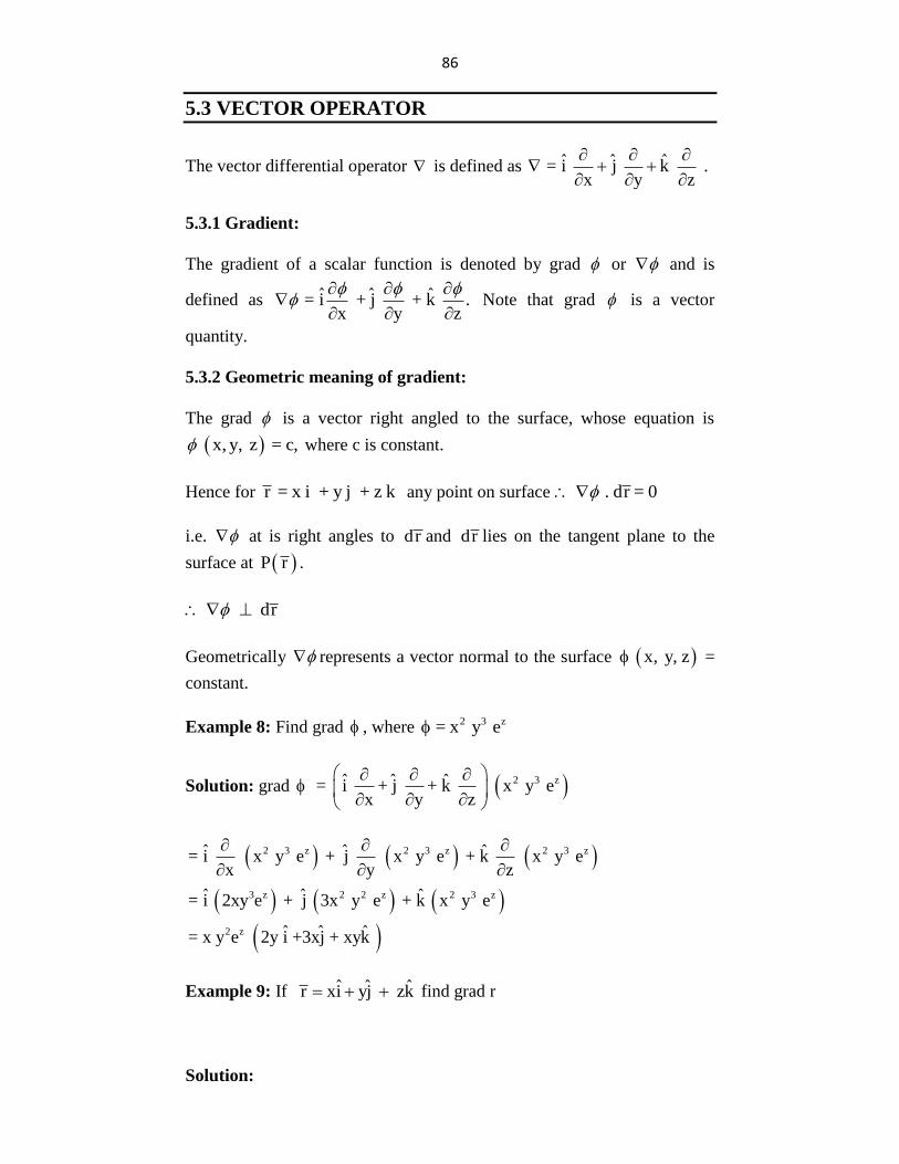
5.3 VECTOR OPERATOR

The vector differential operator

is defined as ˆ ˆ ˆ = i j k x y z

.

5.3.1 Gradient:

The gradient of a scalar function is denoted by grad or and is

defined as ˆ ˆ ˆ = i + j + k .x y z

Note that grad is a vector

quantity.

5.3.2 Geometric meaning of gradient:

The grad is a vector right angled to the surface, whose equation is

x, y, z = c, where c is constant.

Hence for r = x i + y j + z k any point on surface . dr = 0

i.e. at is right angles to dr and dr lies on the tangent plane to the

surface at P r .

dr

Geometrically represents a vector normal to the surface x, y, z =

constant.

Example 8: Find grad , where 2 3 z = x y e

Solution: grad 2 3 zˆ ˆ ˆ= i + j + k x y ex y z

2 3 z 2 3 z 2 3 z

3 z 2 2 z 2 3 z

2 z

ˆ ˆ ˆ= i x y e + j x y e + k x y ex y z

ˆ ˆ ˆ= i 2xy e + j 3x y e + k x y e

ˆ ˆ ˆ= x y e 2y i +3xj + xyk

Example 9: If ˆ ˆ ˆr xi yj zk find grad r

Solution:

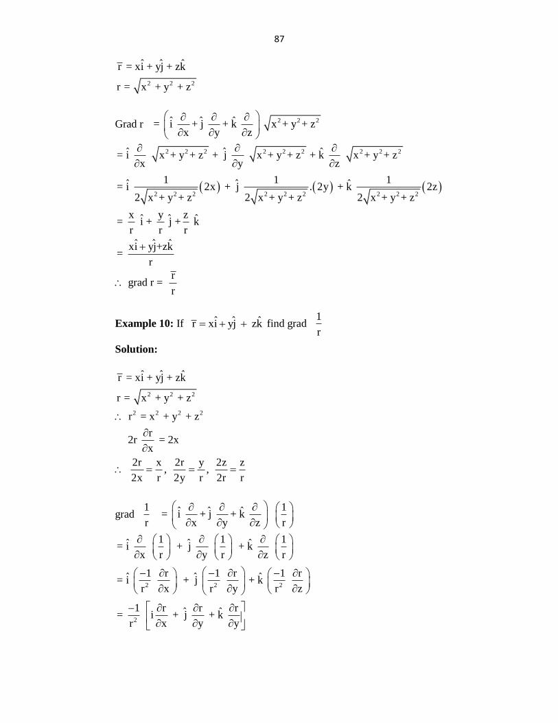
87

2 2 2

ˆ ˆ ˆr = xi + yj + zk

r = x + y + z

Grad r 2 2 2ˆ ˆ ˆ = i + j + k x + y + z

x y z

2 2 2 2 2 2 2 2 2

2 2 2 2 2 2 2 2 2

ˆ ˆ ˆ= i x + y + z + j x + y + z + k x + y + zx y z

1 1 1ˆ ˆ ˆ= i 2x + j . 2y + k 2z2 x + y + z 2 x + y + z 2 x + y + z

x y zˆ ˆ ˆ= i + j + k r r r

ˆ ˆ ˆxi yj+zk=

r

grad r =r

r

Example 10: If ˆ ˆ ˆr xi yj zk find grad 1

r

Solution:

2 2 2

2 2 2 2

ˆ ˆ ˆr = xi + yj + zk

r = x + y + z

r = x + y + z

r 2r = 2x

x

2r x 2r y 2z z , ,

2x r 2y r 2r r

grad 1

r

1ˆ ˆ ˆ = i + j + k x y z r

2 2 2

2

1 1 1ˆ ˆ ˆ= i + j + k x r y r z r

1 r 1 r 1 rˆ ˆ ˆ= i + j + k r x r y r z

1 r r rˆ ˆ= i + j + k r x y y

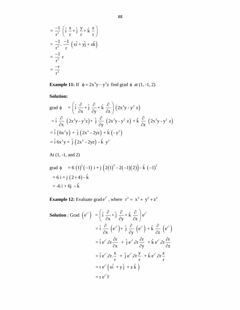
88

2

2

3

3

1 x y zˆ ˆ ˆ= i + j + k r r r r

1 1 ˆ ˆ ˆ= . xi + yj + zkr r

1= r

r

r=

r

Example 11: If 3 22x y y z find grad at (1, -1, 2)

Solution:

grad 3 2ˆ ˆ ˆ= i + j + k 2x y - y zx y z

3 2 3 2 3 2

2 3 2

2 3 2

ˆ ˆ ˆ = i 2x y - y z + j 2x y - y z + k 2x y - y zx y z

ˆ ˆ ˆ= i 6x y + j 2x - 2yz + k - y

ˆ ˆ ˆ= i 6x y + j 2x - 2yz - k y

At (1, -1, and 2)

grad 2 3 2ˆ= 6 1 1 i + j 2 1 2 1 2 k 1

ˆ = 6 i + j 2 4 k

ˆ = -6 i + 6j k

Example 12: Evaluate grad2re , where 2 2 2 2r x y z

Solution : Grad 2re

2rˆ ˆ ˆ = i + j + k ex y z

2 2 2

2 2 2

2 2 2

2

2

r r r

r r r

r r r

r

r

ˆ ˆ ˆ= i e + j e + k ex y z

r r rˆ ˆ ˆ= i e . r + j e . r + k e . rx y z

x y zˆ ˆ ˆ= i e . r. + j e . r + k e . rr r r

ˆ ˆ ˆ= r e xi + y j + z k

= r e r

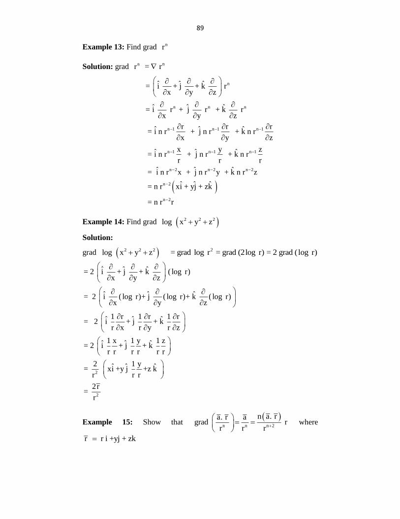
89

Example 13: Find grad nr

Solution: grad nr n= r

n

n n n

ˆ ˆ ˆ= i + j + k r x y z

ˆ ˆ ˆ= i r + j r + k r x y z

n 1 n 1 n 1

n 1 n 1 n 1

n 2 n 2 n 2

n 2

n 2

r r rˆ ˆ ˆ= i n r + j n r + k n rx y z

x y zˆ ˆ ˆ= i n r + j n r + k n rr r r

ˆ ˆ ˆ= i n r x + j n r y + k n r z

ˆ ˆ ˆ= n r xi + yj + zk

= n r r

Example 14: Find grad 2 2 2log x y z

Solution:

grad 2 2 2log x y z 2= grad log r = grad (2log r) = 2 grad ( log r)

2

ˆ ˆ ˆ= 2 i + j + k ( log r)x y z

ˆ ˆ ˆ= 2 i ( log r)+ j ( log r)+ k ( log r) x y z

1 r 1 r 1 rˆ ˆ ˆ= 2 i + j + k r x r y r z

1 x 1 y 1 zˆ ˆ ˆ= 2 i + j + k r r r r r r

2 1 yˆ ˆ ˆ= xi +y j +z k r r r

2

2r=

r

Example 15: Show that

n n n 2

n a. ra. r agrad r

r r r

where

r r i +yj + zk

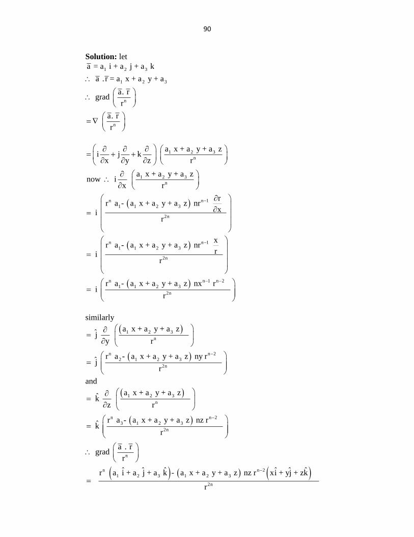
90

Solution: let

1 2 3

1 2 3

n

n

a = a i + a j + a k

a . r = a x + a y + a

a. r grad

r

a. r

r

1 2 3

n

1 2 3

n

n n 1

1 1 2 3

2n

a x + a y + a zi j k

x y z r

a x + a y + a znow i

x r

rr a - a x + a y + a z nr

x i r

n n 1

1 1 2 3

2n

n n 1 n 2

1 1 2 3

2n

xr a - a x + a y + a z nr

r i r

r a - a x + a y + a z nx r i

r

similarly

1 2 3

n

n n 2

2 1 2 3

2n

a x + a y + a z j

y r

r a - a x + a y + a z ny r j

r

and

1 2 3

n

n n 2

3 1 2 3

2n

n

n n 2

1 2 3 1 2 3

2n

a x + a y + a z ˆ k z r

r a - a x + a y + a z nz r ˆ k r

a . r grad

r

ˆ ˆ ˆ ˆ ˆ ˆr a i + a j + a k - a x + a y + a z nz r xi + yj + zk

r

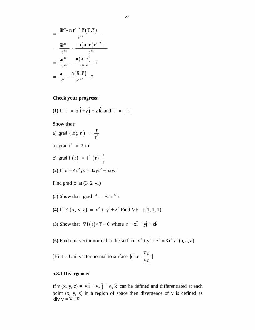
91

n n 2

2n

n 2n

2n 2n

n

2n n 2

n n 2

ar - n r r a . r

r

- n a . r r r ar -

r r

n a . r ar - r

r r

n a . r a - r

r r


(1) If ˆ ˆ ˆr x i +y j + z k

and r r

Show that:

a) 2

rgrad log r

r

b) 3grad r 3 r r

c) 1 r

grad f r f r r

(2) If 2 2 = 4x yz + 3xyz 5xyz

Find grad at (3, 2, -1)

(3) Show that 3 5grad r -3 r r

(4) If 2 2 2F x, y, z x y + z

Find F at (1, 1, 1)

(5) Show that f r r 0 where ˆ ˆ ˆr xi + yj + zk

(6) Find unit vector normal to the surface 2 2 2 2x y z 3a at (a, a, a)

[Hint :- Unit vector normal to surface i.e.

]

5.3.1 Divergence:

If v (x, y, z) = 1 2 3ˆ ˆ ˆv i + v j + v k can be defined and differentiated at each

point (x, y, z) in a region of space then divergence of v is defined as

div v = . v

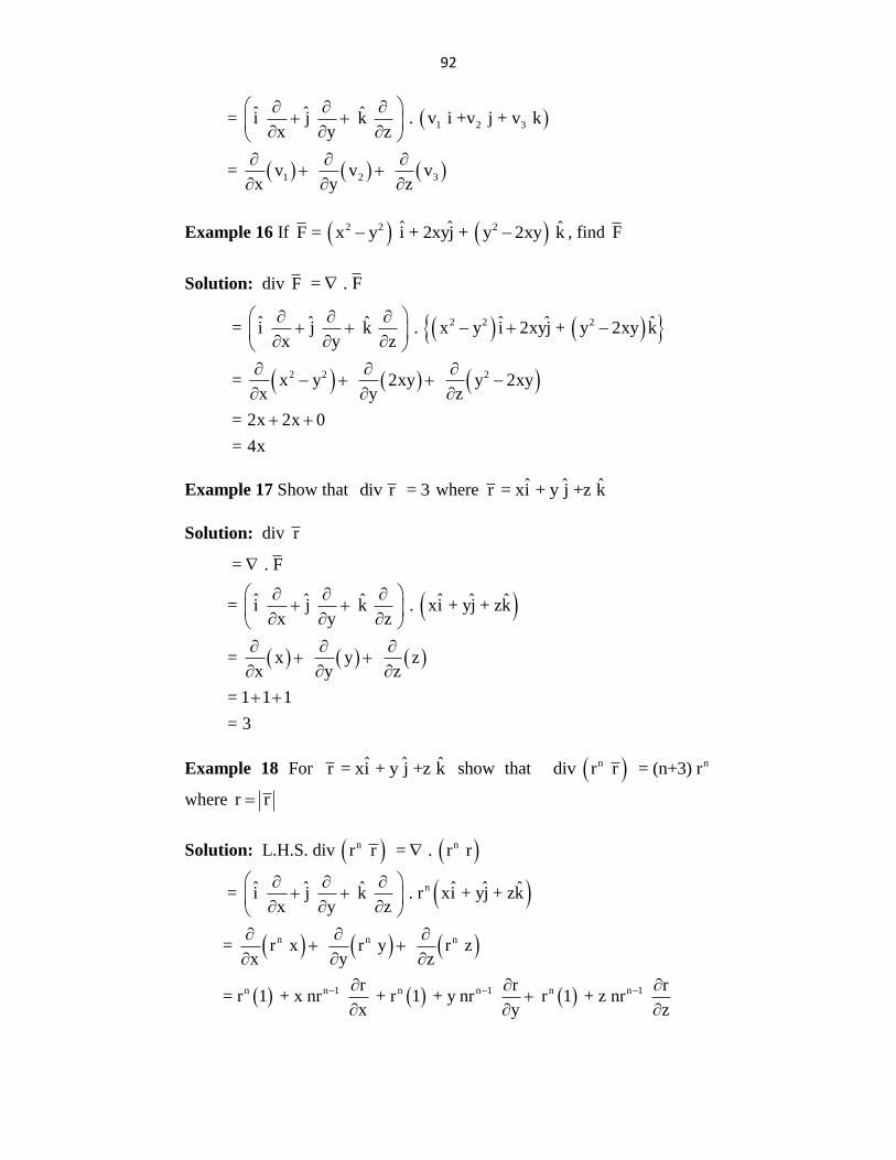
92

1 2 3

1 2 3

ˆ ˆ ˆ = i j k . v i +v j + v kx y z

= v v v x y z

Example 16 If 2 2 2ˆ ˆ ˆF = x y i + 2xyj + y 2xy k ,

find F

Solution: div F = . F

2 2 2

2 2 2

ˆ ˆ ˆ ˆ ˆ ˆ = i j k . x y i 2xyj + y 2xy kx y z

= x y 2xy y 2xy x y z

= 2x 2x 0

= 4x

Example 17 Show that div r = 3

where ˆ ˆ ˆr = xi + y j +z k

Solution: div r

= . F

ˆ ˆ ˆ ˆ ˆ ˆ = i j k . xi + yj + zkx y z

= x y z x y z

= 1 1 1

= 3

Example 18 For ˆ ˆ ˆr = xi + y j +z k show that n ndiv r r = (n+3) r

where r r

Solution: L.H.S. div nr r n = . r r

n

n n n

n n 1 n n 1 n n 1

ˆ ˆ ˆ ˆ ˆ ˆ = i j k . r xi + yj + zk x y z

= r x r y r z x y z

r r r = r 1 + x nr + r 1 + y nr r 1 + z nr

x y z

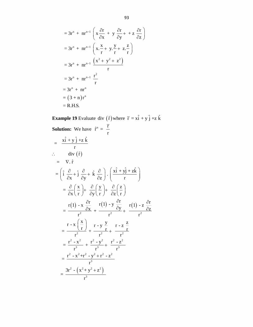
93

n n 1

n n 1

2 2 2

n n 1

2n n 1

n n

n

r r r = 3r + nr x + y + z

x y z

x y z = 3r + nr x. y. z.

r r r

x y z = 3r + nr

r

r = 3r + nr

r

= 3r + nr

= 3 + n r

= R.H.S.

Example 19 Evaluate ˆdiv r where ˆ ˆ ˆr = xi + y j +z k

Solution: We have n r

r = r

2 2

ˆ ˆ ˆxi + y j +z k =

r

ˆ div r

ˆ = . r

ˆ ˆ ˆxi + yj + zkˆ ˆ ˆ = i j k . x y z r

x y z =

x r y r z r

rr r 1 - y r 1 - x yx = +

r r

2

2 2 2

2 2 2 2 2 2

3 3 3

2 2 2 2 2 2

3

2 2 2 2

3

rr 1 - z

z r

x y zr - x r - y r - z r r r = +

r r r

r - x r - y r - z = +

r r r

r - x +r - y r - z =

r

3r - x + y z =

r

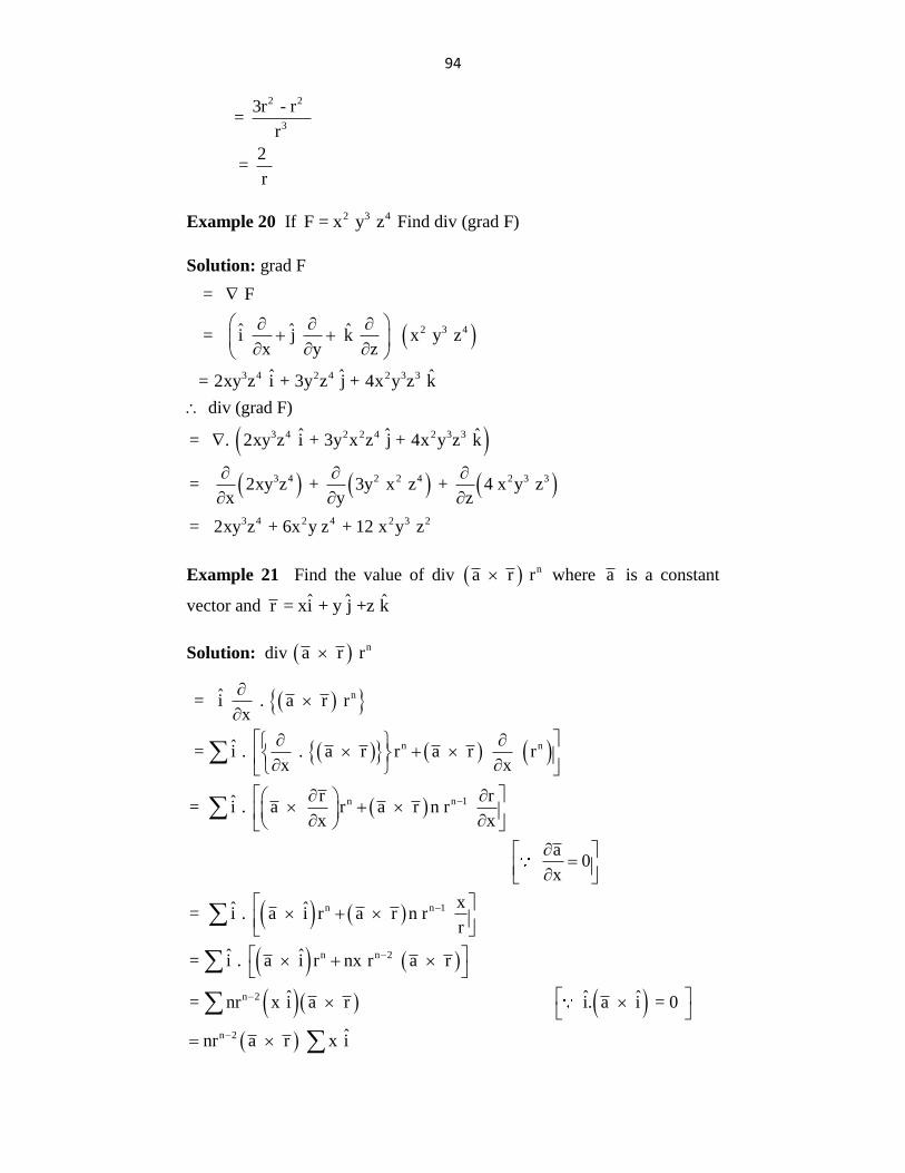
94

2 2

3

3r - r =

r

2 =

r

Example 20 If 2 3 4F = x y z Find div (grad F)

Solution: grad F

2 3 4

3 4 2 4 2 3 3

3 4 2 2 4 2 3 3

3 4 2 2 4 2 3 3

= F

ˆ ˆ ˆ = i j k x y z x y z

ˆ ˆ ˆ = 2xy z i + 3y z j + 4x y z k

div (grad F)

ˆ ˆ ˆ= . 2xy z i + 3y x z j + 4x y z k

= 2xy z + 3y x z + 4 x y zx y z

=

3 4 2 4 2 3 2 2xy z + 6x y z + 12 x y z

Example 21 Find the value of div na r r where a is a constant

vector and ˆ ˆ ˆr = xi + y j +z k

Solution: div na r r

n

n n

n n 1

ˆ = i . a r r x

ˆ = i . . a r r a r rx x

r rˆ= i . a r a r n r x x

a

x

n n 1

n n 2

n 2

n 2

0

xˆ ˆ= i . a i r a r n r r

ˆ ˆ= i . a i r nx r a r

ˆ ˆ ˆ= nr x i a r i. a i = 0

ˆnr a r x i

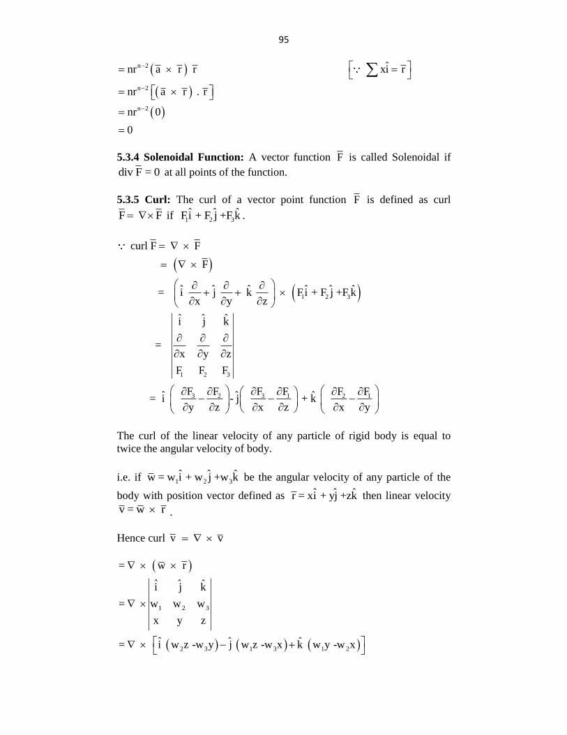
95

n 2

n 2

n 2

ˆnr a r r xi r

nr a r . r

nr 0

0

5.3.4 Solenoidal Function: A vector function F is called Solenoidal if

div F = 0 at all points of the function.

5.3.5 Curl: The curl of a vector point function F is defined as curl

F F if 1 2 3ˆ ˆ ˆFi + F j +F k .

1 2 3

curl F F

F

ˆ ˆ ˆ ˆ ˆ ˆ = i j k F i + F j +F kx y z

1 2 3

3 32 1 2 1

ˆ ˆ î j k

= x y z

F F F

F FF F F Fˆ ˆ ˆ = i - j + k y z x z x y

The curl of the linear velocity of any particle of rigid body is equal to

twice the angular velocity of body.

i.e. if 1 2 3ˆ ˆ ˆw = w i + w j +w k

be the angular velocity of any particle of the

body with position vector defined as ˆ ˆ ˆr = xi + yj +zk then linear velocity

v = w r .

Hence curl

v v

1 2 3

2 3 1 3 1 2

= w r

ˆ ˆ î j k

= w w w

x y z

ˆ ˆ ˆ= i w z -w y j w z -w x k w y -w x

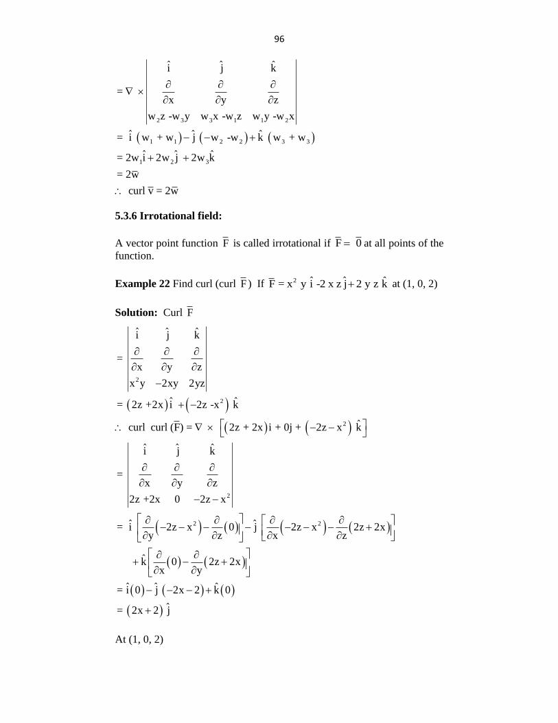
96

2 3 3 1 1 2

1 1 2 2 3 3

1 2 3

ˆ ˆ î j k

= x y z

w z -w y w x -w z w y -w x

ˆ ˆ ˆ= i w + w j w -w k w + w

ˆ ˆ ˆ= 2w i 2w j 2w k

= 2w

curl v = 2w

5.3.6 Irrotational field:

A vector point function F is called irrotational if F 0 at all points of the

function.

Example 22 Find curl (curl F ) If 2 ˆ ˆ ˆF = x y i -2 x z j 2 y z k at (1, 0, 2)

Solution: Curl F

2

2

2

2

2 2

ˆ ˆ î j k

= x y z

x y 2xy 2yz

ˆ ˆ= 2z +2x i 2z -x k

ˆ curl curl (F) = 2z + 2x i + 0j + 2z x k

ˆ ˆ î j k

= x y z

2z +2x 0 2z x

ˆ ˆ= i 2z x 0 j 2z x 2z 2xy z x z

ˆ k 0x

2z 2xy

ˆ ˆ ˆ= i 0 j 2x 2 k 0

ˆ= 2x 2 j

At (1, 0, 2)

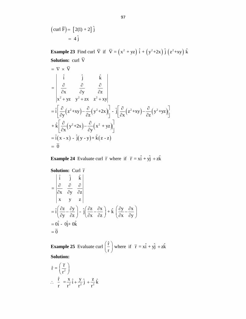
97

ˆcurl F 2(1) + 2 j

ˆ 4 j

Example 23 Find curl V if 2 2 2ˆ ˆ ˆV = x + yz i + y +2x j z +xy k

Solution: curl V

2 2 2

2 2 2 2

V

ˆ ˆ î j k

= x y z

x yz y zx z xy

ˆ î z +xy y +2x - j z +xy y +yzy z x z

2 2ˆ+ k y +2x x + yzx y

ˆ ˆ î x - x - j y - y + k z - z

0

Example 24 Evaluate curl r where if ˆ ˆ ˆr = xi + yj zk

Solution: Curl r

ˆ ˆ î j k

= x y z

x y z

z y z x y xˆ ˆ î - j + k y z x z x y

ˆ ˆ ˆ0i - 0j+ 0k

0

Example 25 Evaluate curl r

r

where if ˆ ˆ ˆr = xi + yj zk

Solution:

2

2 2 2

rr =

r

r x y zˆ ˆ ˆ = i j kr r r r

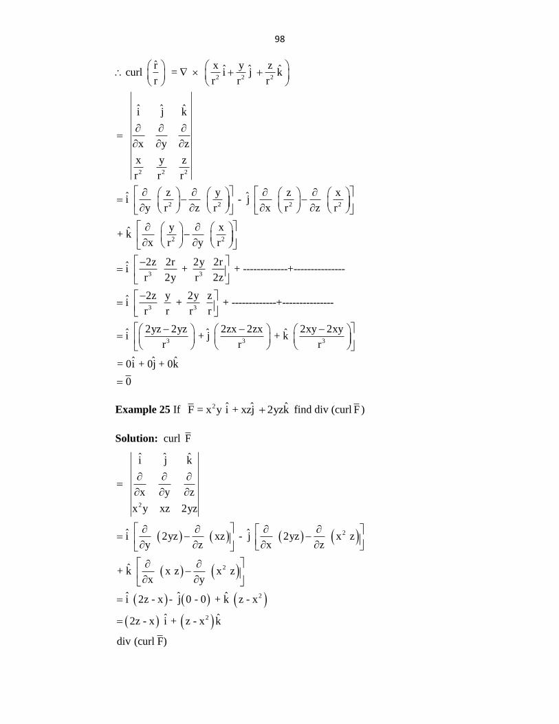
98

2 2 2

2 2 2

2 2 2 2

2 2

3

r x y zˆ ˆ ˆcurl = i j kr r r r

ˆ ˆ î j k

x y z

x y z

r r r

z y z xˆ î - j y r z r x r z r

y xˆ+ k x r y r

2zi

r

3

3 3

3 3 3

2r 2y 2r + + -------------+---------------

2y r 2z

2z y 2y zi + + -------------+---------------

r r r r

2yz 2yz 2zx 2zx 2xy 2xyˆ ˆ î + j + k r r r

ˆ ˆ ˆ= 0i + 0j + 0k

0

Example 25 If 2 ˆ ˆ ˆF = x y i + xzj 2yzk find div (curl F )

Solution: curl F

2

2

2

2

2

ˆ ˆ î j k

x y z

x y xz 2yz

ˆ î 2yz xz - j 2yz x z y z x z

ˆ+ k x z x zx y

ˆ ˆ î 2z - x - j 0 - 0 + k z - x

ˆ ˆ2z - x i + z - x k

div (curl F)

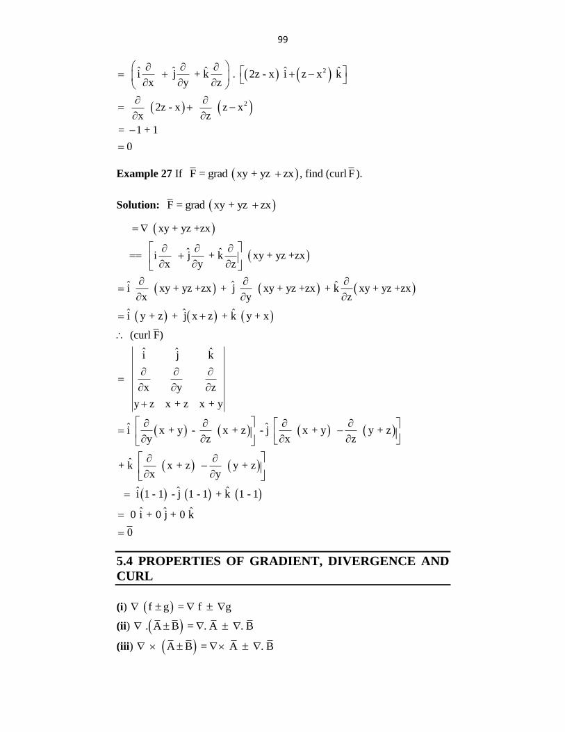
99

2

2

ˆ ˆ ˆ ˆ ˆ i j + k . 2z - x i z x kx y z

2z - x z xx z

= 1 + 1

0

Example 27 If F = grad xy + yz zx , find (curl F ).

Solution: F = grad xy + yz zx

xy + yz +zx

ˆ ˆ i j + k xy + yz +zxx y z

ˆ ˆ î xy + yz +zx + j xy + yz +zx + k xy + yz +zxx y z

ˆ ˆ î y + z + j x z + k y + x

(curl F)

ˆ ˆ î j k

x y z

y z x + z x + y

ˆ î x + y - x + z - j x + y y + z y z x z

ˆ+ k x + z y + zx y

ˆ ˆ ˆ i 1 - 1 - j 1 - 1 + k 1 - 1

ˆ ˆ ˆ 0 i + 0 j + 0 k

0

5.4 PROPERTIES OF GRADIENT, DIVERGENCE AND

CURL

(i) f g = f g

(ii) . A B = . A . B

(iii) A B = A . B

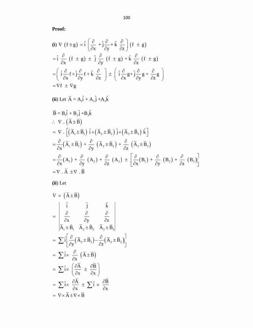
100

Proof:

(i) f g ˆ ˆ î + j + k f gx y z

ˆ ˆ î f g j f g + k f gx y z

ˆ ˆ ˆ ˆ ˆ i f + j f + k i g+ j g + g x y z x y z

f g

(ii) Let 1 2 3ˆ ˆ Â = A i + A j +A k

1 2 3

1 1 2 2 3 3

1 1 2 2 3 3

1 2 3 1 2 3

ˆ ˆ ˆB = B i + B j +B k

. A B

ˆ ˆ ˆ . A B i A B j A B k

A B + A B + A Bx y z

A + A + A B + B + Bx y z x y z

. A . B

(ii) Let

1 1 2 2 3 3

3 3 2 2

A B

ˆ ˆ î j k

x y z

A B A B A B

ˆ i A B A By z

ˆ i A Bx

A Bˆ i x x

A Bˆ ˆ i i x x

A B

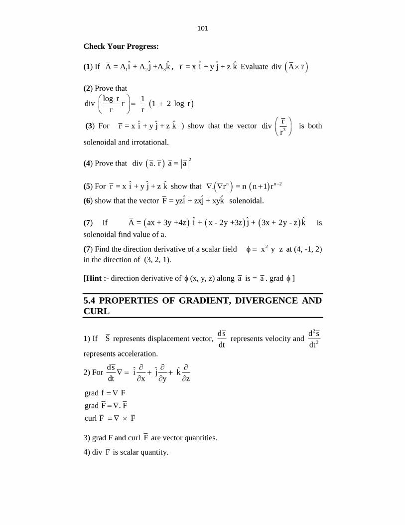
101


(1) If 1 2 3ˆ ˆ Â = A i + A j +A k ,

ˆ ˆ ˆr = x i + y j + z k Evaluate div A r

(2) Prove that

log r 1

div r 1 2 log rr r

(3) For ˆ ˆ ˆr = x i + y j + z k ) show that the vector 3

rdiv

r

is both

solenoidal and irrotational.

(4) Prove that 2

div a. r a = a

(5) For ˆ ˆ ˆr = x i + y j + z k show that n n 2. r = n n 1 r

(6) show that the vector ˆ ˆ ˆF = yzi + zxj + xyk solenoidal.

(7) If ˆ ˆ Â = ax + 3y +4z i + x - 2y +3z j + 3x + 2y - z k is

solenoidal find value of a.

(7) Find the direction derivative of a scalar field 2 x y z at (4, -1, 2)

in the direction of (3, 2, 1).

[Hint :- direction derivative of (x, y, z) along a is = a . grad ]

5.4 PROPERTIES OF GRADIENT, DIVERGENCE AND

CURL

1) If S represents displacement vector, ds

dt represents velocity and

2

2

d s

dt

represents acceleration.

2) For ds ˆ ˆ ˆ i j k dt x y z

grad f F

grad F . F

curl F F

3) grad F and curl F are vector quantities.

4) div F is scalar quantity.

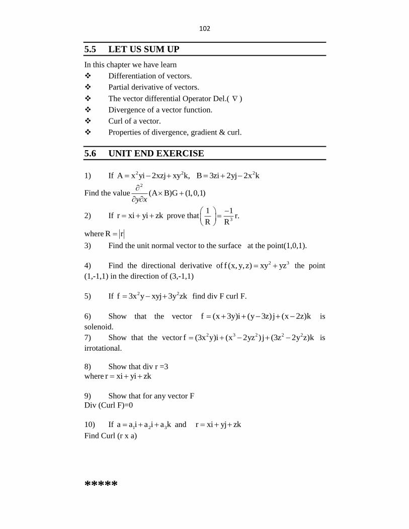
102

5.5 LET US SUM UP


Differentiation of vectors.

Partial derivative of vectors.

The vector differential Operator Del.( )

Divergence of a vector function.

Curl of a vector.

Properties of divergence, gradient & curl.


1) If 2 2A x yi 2xzj xy k,

2B 3zi 2yj 2x k

Find the value2

(A B)G (1,0,1)y x

2) If r xi yi zk prove that3

1 1r.

R R

where R r

3) Find the unit normal vector to the surface at the point(1,0,1).

4) Find the directional derivative of 2 3f (x, y,z) xy yz the point

(1,-1,1) in the direction of (3,-1,1)

5) If 2 2f 3x y xyj 3y zk find div F curl F.

6) Show that the vector f (x 3y)i (y 3z)j (x 2z)k is

solenoid.

7) Show that the vector 2 3 2 2 2f (3x y)i (x 2yz )j (3z 2y z)k is

irrotational.

8) Show that div r =3

where r xi yi zk

9) Show that for any vector F

Div (Curl F)=0

10) If 1 2 3a a i a i a k and

r xi yj zk

Find Curl (r x a)

*****

103

6 DIFFERENTIAL EQUATIONS

UNIT STRUCTURE

6.1 Objective

6.2 Introduction

6.3 Differential Equation

6.4 Formation of differential equation

6.5 Let Us Sum Up


6.1 OBJECTIVE


i. Define differential equation

ii. Order & degree of differential

equation

iii. Formulate the differential equation

6.2 INTRODUCTION

We have already learned differential equation in XIIth . Hence we

are going to discuss differential equation in brief. In this chapter we

discuss only formulation of differential equation.

6.3 DIFFERENTIAL EQUATION

Definition:-

An equation involving independent and dependent variables and the

differential coefficients or differentials is called a differential equation.

e.g. 1 dy

=9dx

x=independent variable

y= depedent variable

2 2

2

d y2 +y=0

dx

dy

dx

3 n

n

d yy=0

dx

104

These are all examples of differential equations.

The differential equation is said to be ordinary if it contains only one

independent variable. All the examples of above are of ordinary

differential equations.

Order and Degree of a Differential Equations:-

(i) Order:-

The order of the differential equations is the order of the highest orderal

derivatives present in the function or equation.

If y = f (x) is a function, then

dy

dx is the first order derivative,

2

2

d y

dx

d dy

dx dx

is the second order derivative.

e.g 1) 2

2

d y2 0

dx

dyy

dx

Order = 2

2) E = Ri + L di

dt

Order = 1

Degree:-

The degree of differential equation is the degree of the highest ordered

derivative in the equation when it is made free from radicals and fractions.

e.g.

1 2

2

2

d y0

dxk y

order = 2, degree = 1

2

22

2

d y2 0

dx

dyY

dx

Order =2, degree =1

3 1

dy

y xdydx

dx

Order=1, degree=2

4 2

32

dy

dx

dy

dx

1 12 3 2

2

d

y dy

dx dx

Cubing both sides

105

3 22

2

dy

dx

yd

dx

Squaring both sides 2 32

2

dy

dx

yd

dx

Order=2, degree=2

Solved examples:

Example 1: Find the order and degree of the following

32 2

2

2

1

i)

dy

dxe

d y

dx

Solution:

32 22

2 e 1

d y dy

dx dx

Squaring both sides

32 222

2 e 1

d y dy

dx dx

order = 2, degree = 2

ii)

32

3sin( ) xd d y

x xy edx dx

Solution:

3 23 3 4

3 3 4

d x 3 sin( )

yxd y d y

xy edx dx dx

Order = 4, degree=1

iii) 5

dy

y xdydx

dx

Solution:

2dy

y 5dy

xdx dx

Order =1, degree=2

106

iv)

2

5 1dy dy

y xdx dx

Solution:

2dy

y x 5 1dy

dx dx

Squaring on both sides

2 2dy

y-x 25 1dx

dy

dx

2 2

2 2 y 2 25 1dy dy dy

xy xdx dx dx

Order =1, degree=2


1) 2

2

u uu

x y

Ans : order =2, degree=1

2)

4 7 113 3 2

3 3 25 7 xd y d y d y dy

y edx dx dx dx

Ans : order=3, degree=7

3) 3 4

11 1 xy y e


4) 11

111

xy

y


5) 11 121y y


2

1 1y x y xy

Ans : order =1, degree=3

6.4 FORMATION OF DIFFERENTIAL EQUATION

Formation of differential equation involves elimination of arbitrary

consonants, in the relation of the variables.

Consider

107

2 1y ax

Where y= independent variable

x = dependent variable

Differentiating equation (1) with respect to x

we have dy

2 (2)dx

ax

From equation (1) we have

2

ya

x

Put value of a in equation (2), we have

2

dy 2

yx

dx x

dy 2

dx

y

x

dy

x 2dx

y

dy

x 2 0dx

y

This is the required differential equation

Note:-

To eliminate two arbitrary constants, three equations are required. To

eliminate three arbitrary constants, four equations are required.

In general to eliminate n arbitrary constants. (n+1) equations are required.

In other words elimination of n arbitrary consonants will bring us to

differential equation of nth order.

Solved Examples:-

Example 2: Form the differential equations if 1 2cos siny c x c x

Solution: We have

Y= c1 cos x + c 2 sinx -------------(1)

This equation contains two arbitrary constants, therefore we shall require

three equations to eliminate c1 and c 2 .

Differentiating equation (1) with respect to x

1 2

dy = -c cos cos .dx

x c x

Again differentiate with respect to x

2

1 22

d = -c cos sin

dx

yx c x

108

2

1 22

d = (c cos +c sin )

yx x

dx

2

2

d = ----(1)

yy from eq

dx

2

2

d + y = 0

dx

y

This is the required differential equation.

Example 3: Form the differential equation from

x= a sin (wt+c) where a and c are arbitrary constants.

Solution: We have,

x= a sin (wt+c)--------(1)

Differentiate equation (1) with respect

dx

+ acos (cot+c) wdt

dx

+ aw cos(cot+c) dt

Again differentiating w.r.t. 't'

2

2

d x -a wsin cot c w

dt

2

2

2

d x -w a sin cot c

dt

2

2

2

d x - ........ sin equation 1w x u g

dt

22

2

d xw x 0

dt

This is the required differential equation

Example 4: From the differential equation if y= log (ax)

Solution:

log( ) (1)y ax

Differentiate equation (1) with respect to x .

dy 1

dx

AAx

dy 1

dx x

dy

x 1dx


109

Example 5: Obtain the differential equation for the equation Y=cx+ c2

Solution: we have,

2 (1)y cx c

Differentiate equation (1) with repect to x

dy

dx

c

Put value of c in equation (1)

2dy dy

y= xdx dx


Example 6: Obtain the differential equation for the relation 2x 3 y= a e a,b are constants.xb e Where

Solution: we have,

2x 3 y= a e -------------(1).xb e

Here the number of arbitrary constants is two

Hence we shall require three equations to

Eliminate and b. So we differentiate the given equations twice.

2x 3dy

= 2a e 3 -------------(2).dx

xb e

2

2x 3

2

d y = 4a e 9 -------------(3)dx

xb e

From equation (1) (2) & (3) elimination of a & b gives directly

2

2

1 1

dy 2 3 0dx

4 9

y

d y

dx

In the determinant

1st column is LHS

Column 2nd column 2nd column contains coefficients 2xa e

Expanding the determinant

2nd column contains coefficients of 3xb e

2

218 12 9 4 3 2 0

dy d yy

dx dx

2

2

dy d y 6y-5 0

dx dx

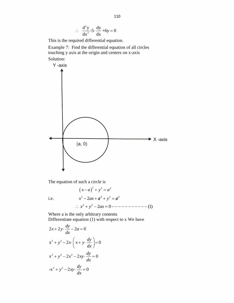
110

2

2

d y dy -5 +6y 0dx dx


Example 7: Find the differential equation of all circles

touching y axis at the origin and centers on x-axis

Solution:

The equation of such a circle is

2 2 2 x a y a

i.e. 2 2 2 2 2x ax a y a

2 2 2 0 (1)x y ax

Where a is the only arbitrary contents

Differentiate equation (1) with respect to x We have

2 2 2 0dy

x y adx

2 2x 2 0dy

y x x ydx

2 2 2x 2 2 0dy

y x xydx

2 2-x 2 0dy

y xydx

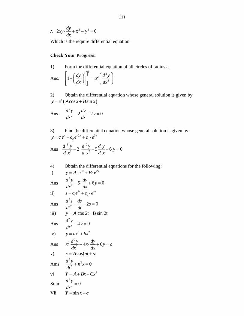
111

2 2 2 x 0dy

xy ydx

Which is the require differential equation.


1) Form the differential equation of all circles of radius a.

Ans.

32 2

2

21

dy d ya

dx dx

2) Obtain the differential equation whose general solution is given by

cos sinxy e A x B x

Ans 2

22 2 0

d y dyy

dx dx

3) Find the differential equation whose general solution is given by 2 3

1 2 3

x x xy c e c e c e

Ans 3 2

3 2

2 5 6 0

d y d y d yy

d x d x d x

4) Obtain the differential equations for the following:

i) 3 2x xy A e B e

Ans 2

25 6 0

d y dyy

dx dx

ii) 2

1 2

t ts c e c e

Ans 2

22 0

d s dss

dt dt

iii) cos 2t+ B sin 2ty A

Ans 2

2

d4 0

yy

dt

iv) 3 2y ax bx

Ans 2

2

24 6

d y dyx x y o

dx dx

v) cos(x A nt

Ams 2

2

20

d yn x

dt

vi 2Y A Bx Cx

Soln 2

20

d y

dx

Vii sinY x c

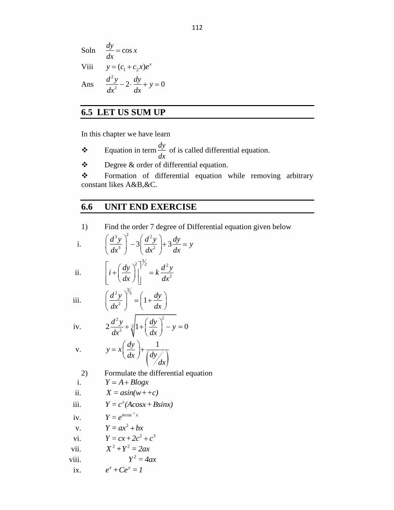
112

Soln cosdy

xdx

Viii 1 2( ) xy c c x e

Ans 2

22 0

d y dyy

dx dx

6.5 LET US SUM UP


Equation in termdy

dx of is called differential equation.

Degree & order of differential equation.

Formation of differential equation while removing arbitrary

constant likes A&B,&C.


1) Find the order 7 degree of Differential equation given below

i.

23 2

3 23 3

d y d y dyy

dx dx dx

ii.

32 2 2

2

dy d yi k

dx dx

iii.

32 5

21

d y dy

dx dx

iv.

22

32

2 1 0d y dy

ydx dx

v.

1dy

y xdydx

dx

2) Formulate the differential equation

i. Y A Blogx

ii. X = asin(w++c)

iii. xY = c (Acosx+Bsinx)

iv. 1cosm xY = e

v. 2Y = ax bx

vi. 2 3Y = cx+2c c

vii. 2 2X +Y = 2ax

viii. 2Y = 4ax

ix. x ye +Ce = 1

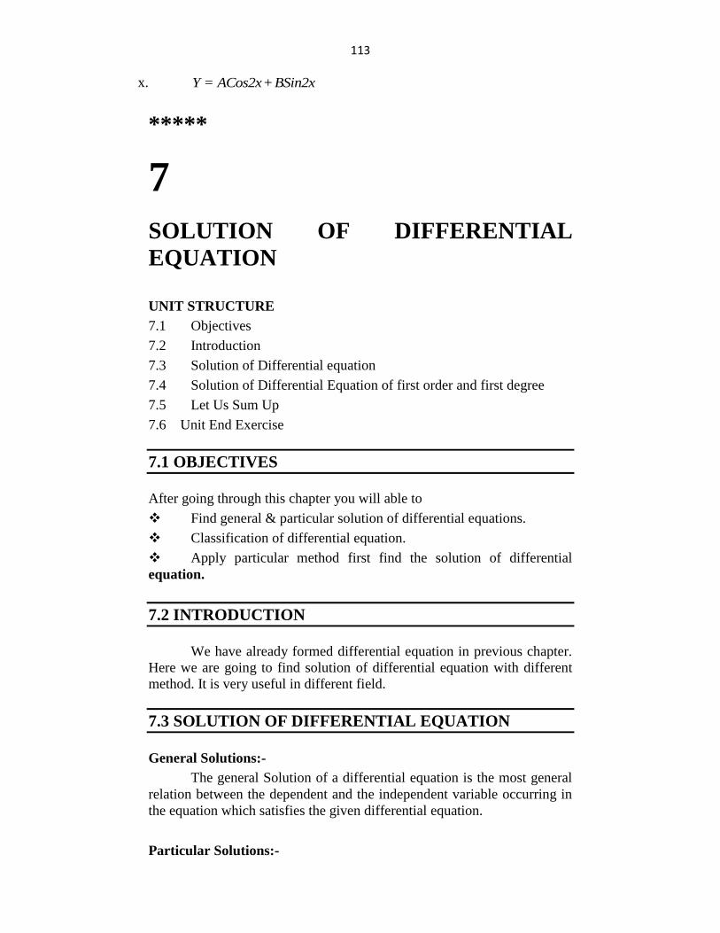
113

x. Y = ACos2x+BSin2x

*****

7

SOLUTION OF DIFFERENTIAL

EQUATION

UNIT STRUCTURE

7.1 Objectives

7.2 Introduction

7.3 Solution of Differential equation

7.4 Solution of Differential Equation of first order and first degree

7.5 Let Us Sum Up


7.1 OBJECTIVES


Find general & particular solution of differential equations.

Classification of differential equation.

Apply particular method first find the solution of differential

equation.

7.2 INTRODUCTION

We have already formed differential equation in previous chapter.

Here we are going to find solution of differential equation with different

method. It is very useful in different field.

7.3 SOLUTION OF DIFFERENTIAL EQUATION

General Solutions:-

The general Solution of a differential equation is the most general

relation between the dependent and the independent variable occurring in

the equation which satisfies the given differential equation.

Particular Solutions:-

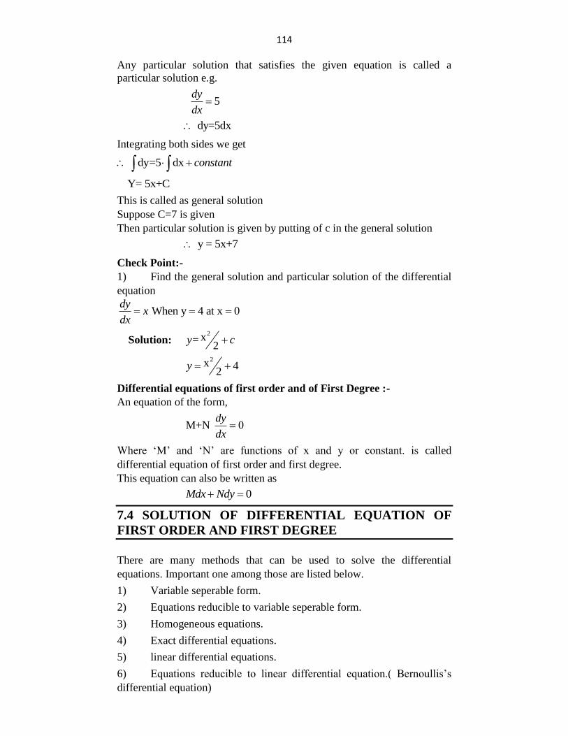
114

Any particular solution that satisfies the given equation is called a

particular solution e.g.

5dy

dx

dy=5dx

Integrating both sides we get

dy=5 dx constant

Y= 5x+C

This is called as general solution

Suppose C=7 is given

Then particular solution is given by putting of c in the general solution

y = 5x+7

Check Point:-

1) Find the general solution and particular solution of the differential

equation

When y 4 at x 0dy

xdx

Solution: 2x=

2y c

2x 4

2y

Differential equations of first order and of First Degree :-

An equation of the form,

M+N 0dy

dx

Where „M‟ and „N‟ are functions of x and y or constant. is called

differential equation of first order and first degree.

This equation can also be written as

0Mdx Ndy

7.4 SOLUTION OF DIFFERENTIAL EQUATION OF

FIRST ORDER AND FIRST DEGREE

There are many methods that can be used to solve the differential

equations. Important one among those are listed below.

1) Variable seperable form.

2) Equations reducible to variable seperable form.

3) Homogeneous equations.

4) Exact differential equations.

5) linear differential equations.

6) Equations reducible to linear differential equation.( Bernoullis‟s

differential equation)

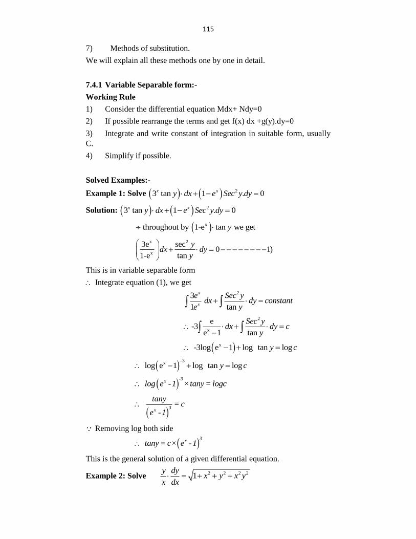
115

7) Methods of substitution.

We will explain all these methods one by one in detail.

7.4.1 Variable Separable form:-

Working Rule

1) Consider the differential equation Mdx+ Ndy=0

2) If possible rearrange the terms and get f(x) dx +g(y).dy=0

3) Integrate and write constant of integration in suitable form, usually

C.

4) Simplify if possible.

Solved Examples:-

Example 1: Solve 23 tan 1 . 0x xy dx e Sec y dy

Solution: 23 tan 1 . 0x xy dx e Sec y dy

x throughout by 1-e tan we get y

x 2

x

3e sec0 1)

1-e tan

ydx dy

y

This is in variable separable form

Integrate equation (1), we get

23

1 tan

x

x

e Sec ydx dy constant

e y

2

x

e-3

e 1 tan

Sec ydx dy c

y

x -3log e 1 log tan logy c

3

x log e 1 log tan logy c

-3

xlog e -1 ×tany = logc

3x

tany= c

e -1

Removing log both side

3

xtany = c× e -1

This is the general solution of a given differential equation.

Example 2: Solve 2 2 2 21

y dyx y x y

x dx

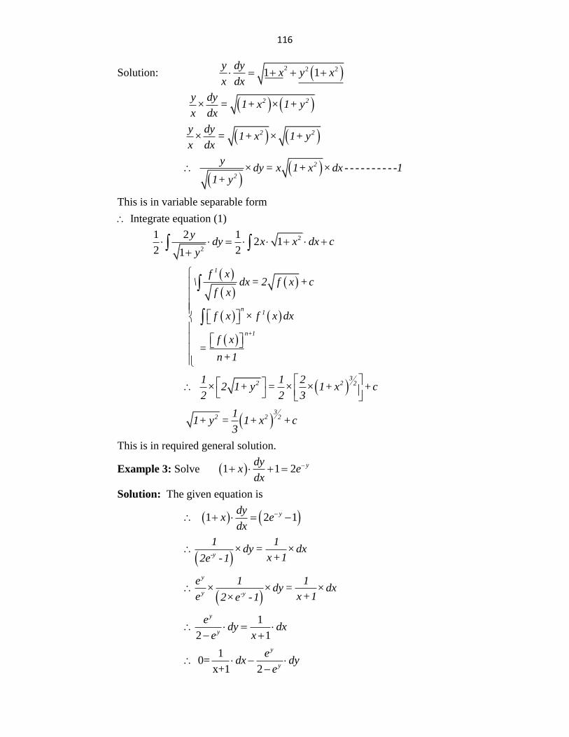
116

Solution: 2 2 21 1y dy

x y xx dx

2 2y dy × = 1+ x × 1+ yx dx

2 2y dy× = 1+ x × 1+ y

x dx

2

2

y×dy = x 1+ x ×dx - - - - - - - - - -1

1+ y


Integrate equation (1)

2

2

1 2 12 1

2 21

ydy x x dx c

y

1

n1

n+1

f x\ dx = 2 f x +c

f x

f x × f x dx

f x =

n+1

3

2 2 21 1 2× 2 1+ y = × × 1+ x +c

2 2 3

3

2 2 211+ y = 1+ x +c

3

This is in required general solution.

Example 3: Solve 1 1 2 ydyx e

dx

Solution: The given equation is

1 2 1ydyx e

dx

-y

1 1 ×dy = ×dx

x+12e -1

y

y -y

e 1 1 × ×dy = ×dxe x+12×e -1

1

2 1

y

y

edy dx

e x

1

0=x+1 2

y

y

edx dy

e

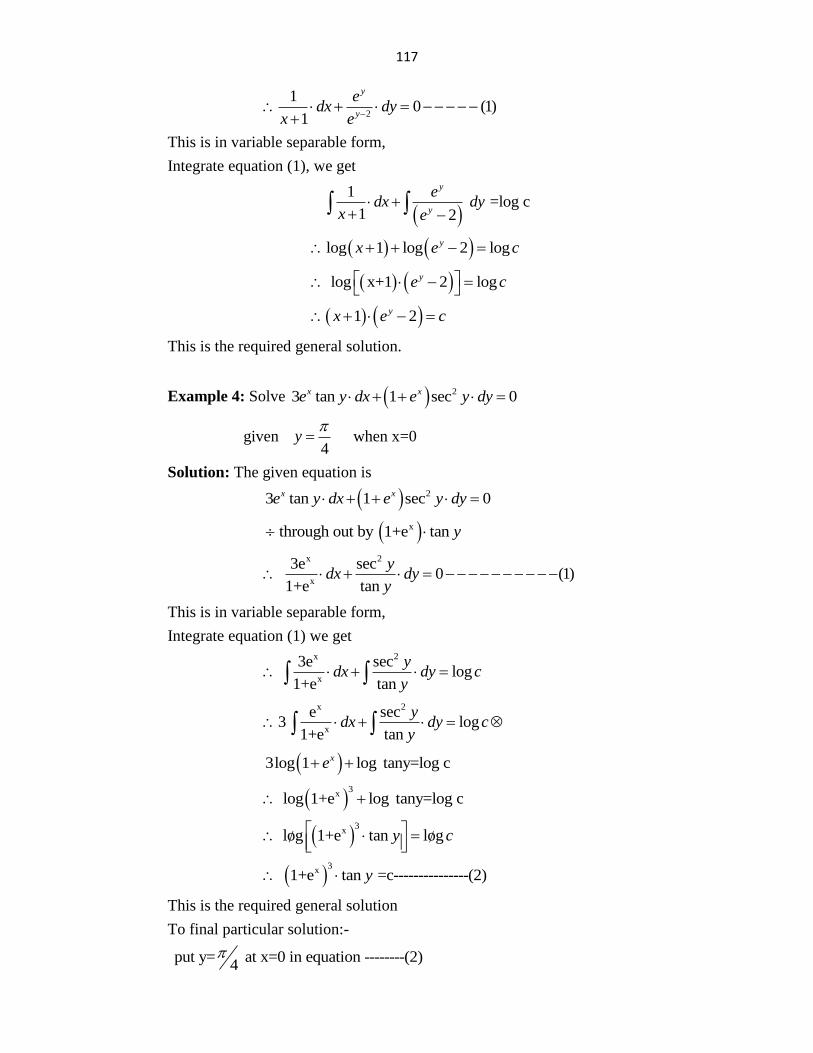
117

2

10 (1)

1

y

y

edx dy

x e

This is in variable separable form,


1 =log c

1 2

y

y

edx dy

x e

log 1 log 2 logyx e c

log x+1 2 logye c

1 2yx e c

This is the required general solution.

Example 4: Solve 23 tan 1 sec 0x xe y dx e y dy

given 4

y

when x=0


23 tan 1 sec 0x xe y dx e y dy

x through out by 1+e tan y

x 2

x

3e sec 0 (1)1+e tan

ydx dy

y

This is in variable separable form,

Integrate equation (1) we get

x 2

x

3e sec log

1+e tan

ydx dy c

y

x 2

x

e sec3 log

1+e tan

ydx dy c

y

3log 1 log tany=log cxe

3

x log 1+e log tany=log c

3

x log 1+e tan logy c

3

x 1+e tan =c---------------(2)y

This is the required general solution

To final particular solution:-

put y= at x=0 in equation --------(2)4

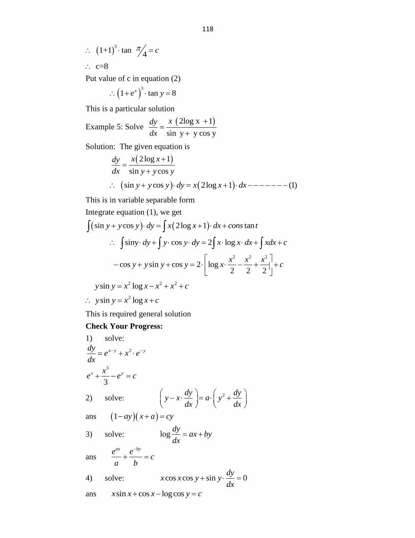
118

3

1+1 tan 4

c

c=8

Put value of c in equation (2)

3

1 tan 8xe y

This is a particular solution

Example 5: Solve 2log x 1

sin y y cos y

xdy

dx


2log 1

sin cos

x xdy

dx y y y

sin cos 2log 1 (1)y y y dy x x dx



sin cos 2log 1 tany y y dy x x dx cons t

siny cos 2 logdy y y dy x x dx xdx c

2 2 2

cos sin cos 2 log2 2 2

x x xy y y y x c

2 2 2 sin logy y x x x x c

2 sin logy y x x c

This is required general solution


1) solve:

2x y ydye x e

dx

3

3

x yxe e c

2) solve: 2dy dy

y x a ydx dx

ans 1 ay x a cy

3) solve: logdy

ax bydx

ans ax bye e

ca b

4) solve: cos cos sin 0dy

x x y ydx

ans sin cos logcosx x x y c

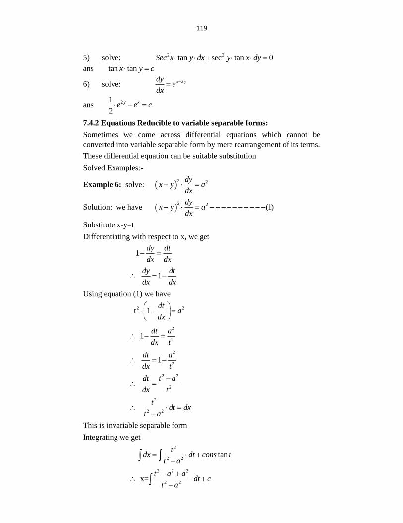
119

5) solve: 2 2tan sec tan 0Sec x y dx y x dy

ans tan tanx y c

6) solve: 2x ydy

edx

ans 21

2

y xe e c

7.4.2 Equations Reducible to variable separable forms:

Sometimes we come across differential equations which cannot be

converted into variable separable form by mere rearrangement of its terms.

These differential equation can be suitable substitution

Solved Examples:-

Example 6: solve: 2 2dy

x y adx

Solution: we have 2 2 (1)

dyx y a

dx

Substitute x-y=t

Differentiating with respect to x, we get

1dy dt

dx dx

1dy dt

dx dx

Using equation (1) we have

2 2 t 1

dta

dx

2

2 1

dt a

dx t

2

2 1

dt a

dx t

2 2

2

dt t a

dx t

2

2 2

tdt dx

t a

This is invariable separable form

Integrating we get

2

2 2 tan

tdx dt cons t

t a

2 2 2

2 2 x=

t a adt c

t a

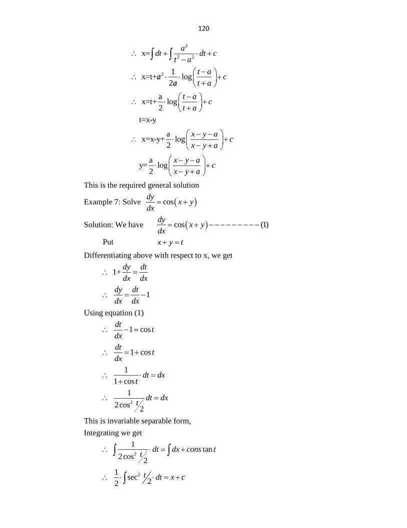
120

2

2 2 x=

adt dt c

t a

2 1

x=t+ log2

t aa c

a t a

a

x=t+ log2

t ac

t a

t=x-y

a

x=x-y+ log2

x y ac

x y a

a

y= log2

x y ac

x y a


Example 7: Solve cosdy

x ydx

Solution: We have cos (1)dy

x ydx

Put x y t

Differentiating above with respect to x, we get

1+dy dt

dx dx

1dy dt

dx dx

Using equation (1)

1 cosdt

tdx

1 cosdt

tdx

1

1 cos

dt dxt

2

1 2cos

2

dt dxt

This is invariable separable form,

Integrating we get

2

1 tan

2cos2

dt dx cons tt

21

sec22

t dt x c

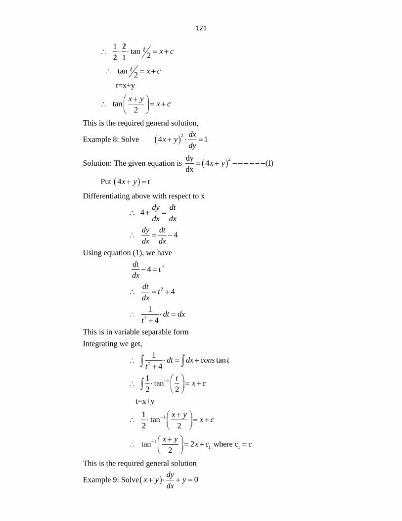
121

1 2

tan22 1

t x c

tan2

t x c

t=x+y

tan2

x yx c

This is the required general solution,

Example 8: Solve 2

4 1dx

x ydy


2dy

4 (1)dx

x y

Put 4x y t

Differentiating above with respect to x

4dy dt

dx dx

4dy dt

dx dx

Using equation (1), we have

24

dtt

dx

2 4

dtt

dx

2

1

4dt dx

t


Integrating we get,

2

1 tan

4dt dx cons t

t

11

tan2 2

tx c

t=x+y

11

tan2 2

x yx c

1

1 1 tan 2 where c2

x yx c c


Example 9: Solve 0dy

x y ydx

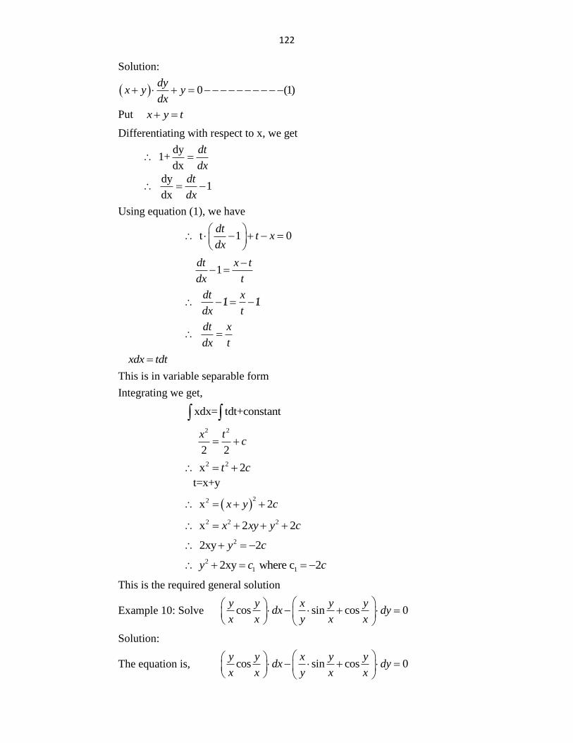
122

Solution:

0 (1)dy

x y ydx

Put x y t

Differentiating with respect to x, we get

dy

1+dx

dt

dx

dy

1dx

dt

dx

Using equation (1), we have

t 1 0dt

t xdx

1dt x t

dx t

1 1dt x

dx t

dt x

dx t

xdx tdt


Integrating we get,

xdx= tdt+constant

2 2

2 2

x tc

2 2 x 2t c

t=x+y

22 x 2x y c

2 2 2 x 2 2x xy y c

2 2xy 2y c

2

1 1 2xy where c 2y c c


Example 10: Solve cos sin cos 0y y x y y

dx dyx x y x x

Solution:

The equation is, cos sin cos 0y y x y y

dx dyx x y x x

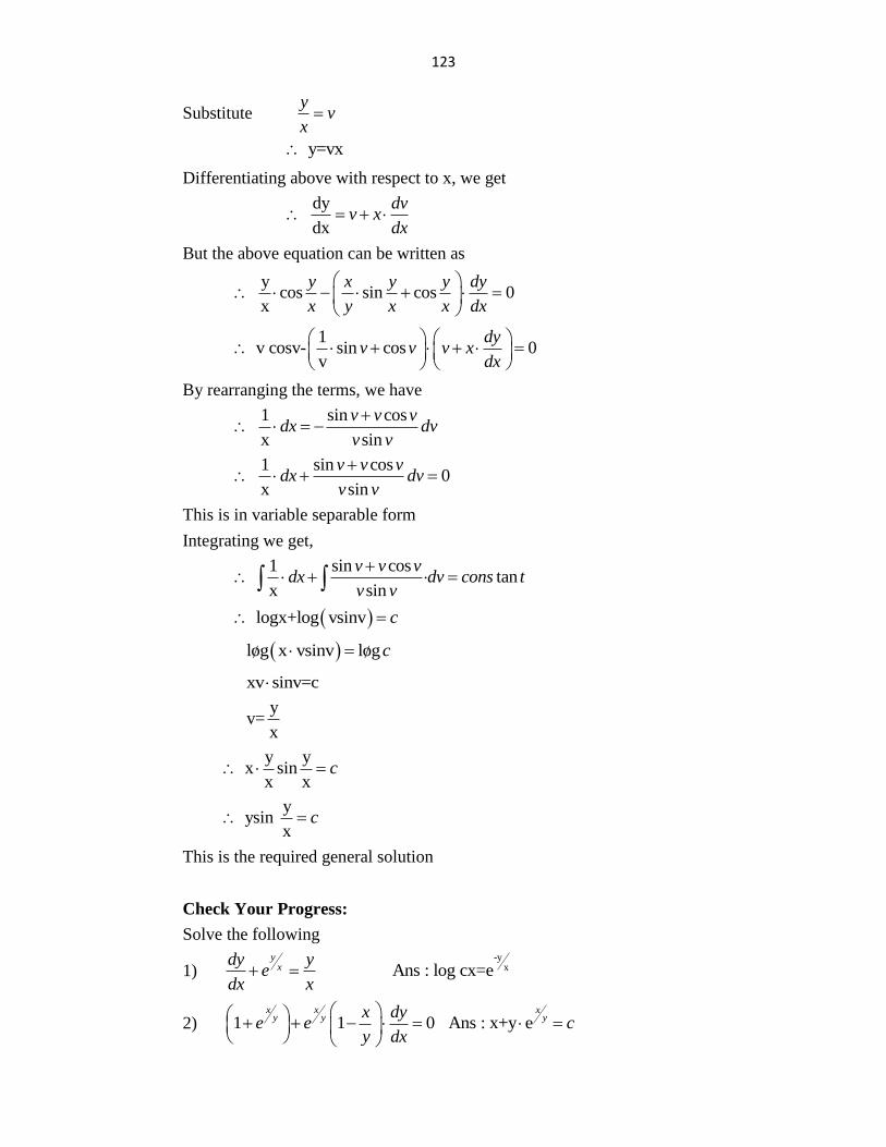
123

Substitute y

vx

y=vx

Differentiating above with respect to x, we get

dy

dx

dvv x

dx

But the above equation can be written as

y

cos sin cos 0x

y x y y dy

x y x x dx

1

v cosv- sin cos 0v

dyv v v x

dx

By rearranging the terms, we have

1 sin cos

x sin

v v vdx dv

v v

1 sin cos

0x sin

v v vdx dv

v v


Integrating we get,

1 sin cos

tanx sin

v v vdx dv cons t

v v

logx+log vsinv c

log x vsinv logc

xv sinv=c

y

v=x

y y

x sinx x

c

y

ysin x

c



Solve the following

1) -y

x Ans : log cx=ey

xdy y

edx x

2) 1 1 0 Ans : x+y ex x x

y y yx dye e c

y dx

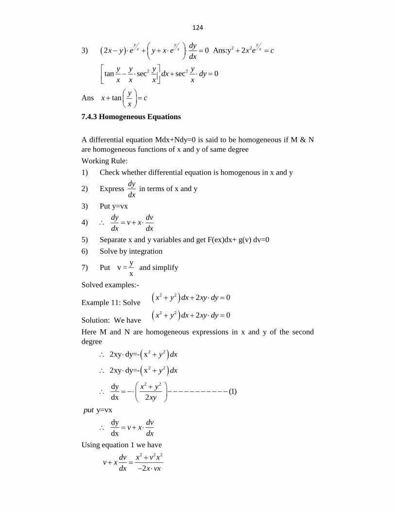
124

3) 2 22 0 Ans:y 2y y y

x x xdy

x y e y x e x e cdx

2 2tan sec sec 0

y y y ydx dy

x x x x

Ans tany

x cx

7.4.3 Homogeneous Equations

A differential equation Mdx+Ndy=0 is said to be homogeneous if M & N

are homogeneous functions of x and y of same degree

Working Rule:

1) Check whether differential equation is homogenous in x and y

2) Express dy

dx in terms of x and y

3) Put y=vx

4) dy dv

v xdx dx

5) Separate x and y variables and get F(ex)dx+ g(v) dv=0

6) Solve by integration

7) Put y

v =x

and simplify

Solved examples:-

Example 11: Solve 2 2 2 0x y dx xy dy

Solution: We have 2 2 2 0x y dx xy dy

Here M and N are homogeneous expressions in x and y of the second

degree

2 2 2xy dy=- x y dx

2 2 2xy dy=- x y dx

2 2dy

(1)dx 2

x y

xy

y=vxput

dy

dx

dvv x

dx

Using equation 1 we have

2 2 2

2

dv x v xv x

dx x vx

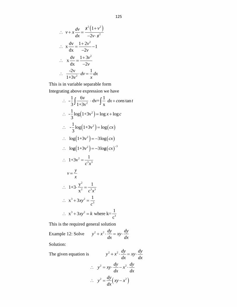
125

2 2

2

1

2

x vdvv x

dx v x

2dv 1 2

x 1dx 2

v

v

2dv 1 3

xdx 2

v

v

2

-2v 1 1+3v

dv dxx


Integrating above expression we have

2

1 6v 1 - dv= tan

3 1+3v xdx cons t

21 - log 1+3v log log

3x c

21 - log 1+3v log

3cx

2 log 1+3v 3log cx

32 log 1+3v 3log cx

2

3 3

1 1+3v

c x

y

vx

2

2 3 3

y 1 1+3

x c x

3 2

3

1 x 3xy

c

3 2

3

1 x 3 where k=

cxy k


Example 12: Solve 2 2 dy dy

y x xydx dx

Solution:

The given equation is 2 2 dy dy

y x xydx dx

2 2

dy dyy xy x

dx dx

2 2 dy

y xy xdx

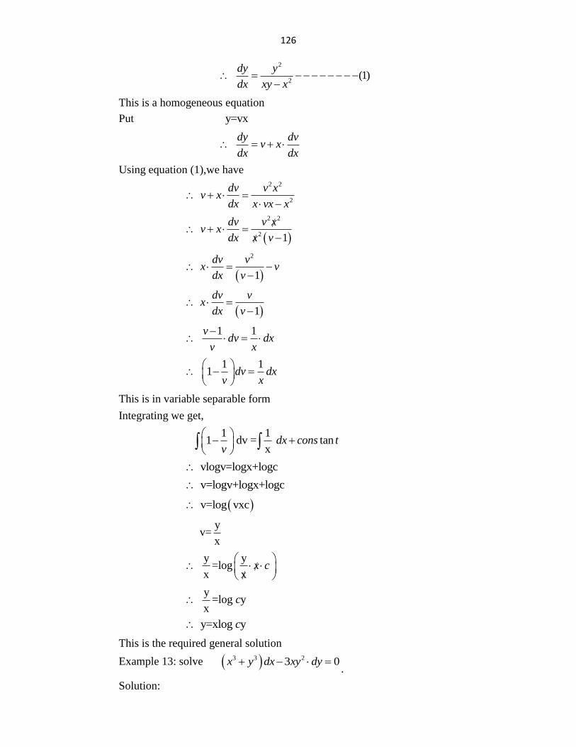
126

2

2 (1)dy y

dx xy x

This is a homogeneous equation

Put y=vx

dy dv

v xdx dx

Using equation (1),we have

2 2

2

dv v xv x

dx x vx x

2 2

2

1

dv v xv x

dx x v

2

1

dv vx v

dx v

1

dv vx

dx v

1 1

v

dv dxv x

1 1

1 dv dxv x


Integrating we get,

1 1

1 dv = tanx

dx cons tv

vlogv=logx+logc

v=logv+logx+logc

v=log vxc

y

v=x

y y

=logx x

x c

y

=log yx

c

y=xlog yc


Example 13: solve 3 3 23 0x y dx xy dy .

Solution:

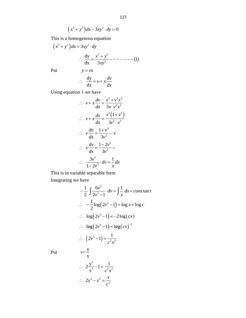
127

3 3 23 0x y dx xy dy

This is a homogenous equation

3 3 2 3x y dx xy dy

3 3

2

dy(1)

dx 3

x y

xy

Put y vx

dy

dx

dvv x

dx


3 3 3

2 2

3

dv x v xv x

dx x v x

3 3

2 3

1

3

x vdvv x

dx v x

3

2

1

3

dv vx v

dx v

3

2

1 2

3

dv vx

dx v

2

3

3 1 1 2

vdv dx

v x


Integrating we have

2

3

1 6 1 tan

2 2 1

vdv dx cons t

v x

31 log 2 1 log log

2v x c

3 log 2 1 2logv cx

23 log 2 1 logv cx

3

2 2

1 2 1v

c x

Put y

v=x

3

3 2 2

y 1 2 1

x c x

3 3

2 2y

xx

c

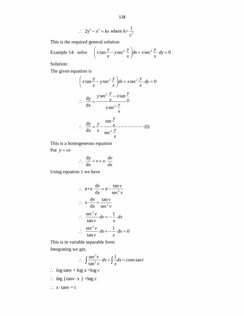
128

3 3

2

1 2y where k=

cx kx


Example 14: solve 2 2tan sec sec 0

y y yx y dx x dy

x x x

Solution:

The given equation is

2 2tan sec sec 0

y y yx y dx x dy

x x x

2

2

sec tandy

dx

sec

y yy x

x xy

xx

2

tandy

(1)dx

sec

y

y xyx

x

This is a homogeneous equation

Put y vx

dy

dx

dvv x

dx


2

dv tan v+x

dx sec

vv

v

2

dv tan x

dx sec

v

v

2sec 1

tan

vdv dx

v x

2sec 1

0tan

vdv dx

v x


Integrating we get,

2

2

sec 1 tan

tan

vdv dx cons t

v x

og tanv + log x =log cl

og tanv x =log cl

x tanv = c

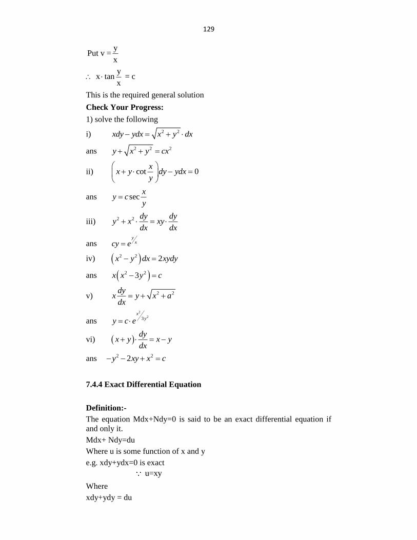
129

yPut v =

x

y x tan = c

x



1) solve the following

i) 2 2xdy ydx x y dx

ans 2 2 2y x y cx

ii) cot 0x

x y dy ydxy

ans secx

y cy

iii) 2 2 dy dy

y x xydx dx

ans y

xcy e

iv) 2 2 2x y dx xydy

ans 2 23x x y c

v) 2 2dy

x y x adx

ans

2

23x

yy c e

vi) dy

x y x ydx

ans 2 22y xy x c

7.4.4 Exact Differential Equation

Definition:-

The equation Mdx+Ndy=0 is said to be an exact differential equation if

and only it.

Mdx+ Ndy=du

Where u is some function of x and y

e.g. xdy+ydx=0 is exact

u=xy

Where

xdy+ydy = du

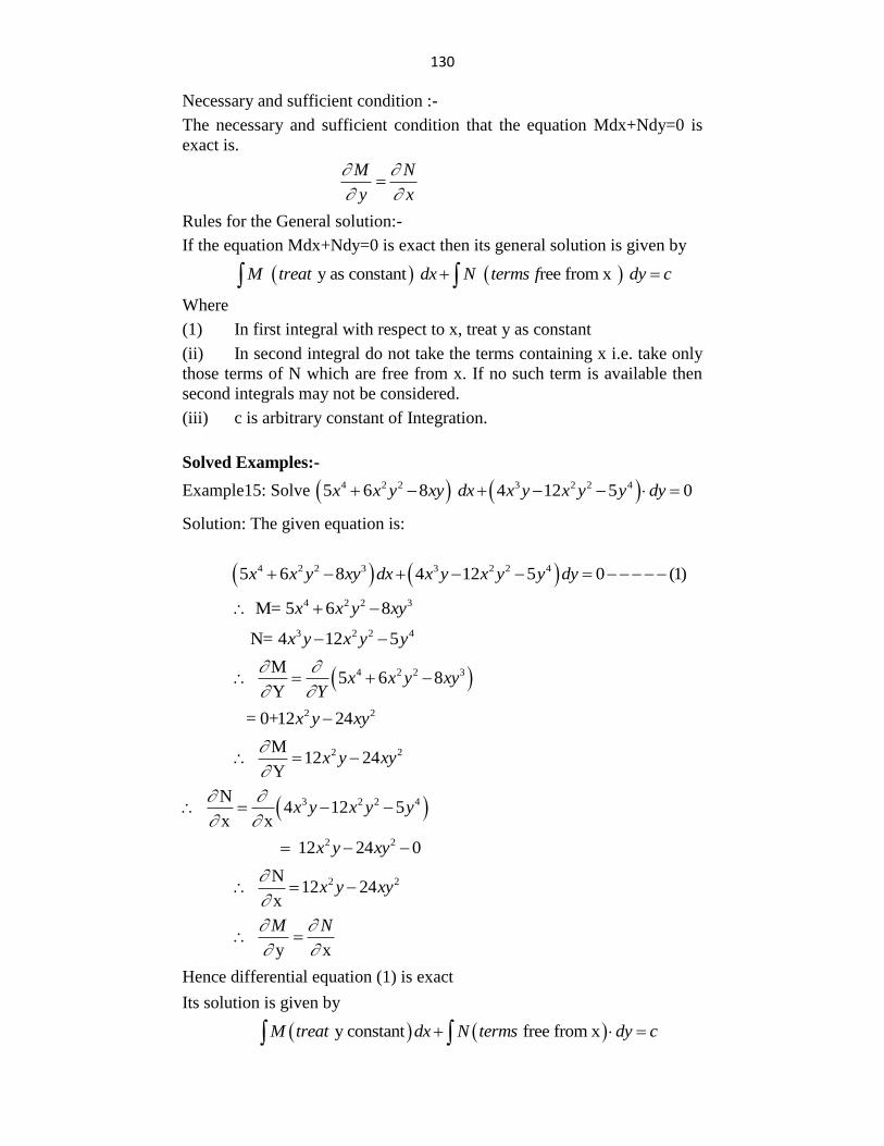
130

Necessary and sufficient condition :-

The necessary and sufficient condition that the equation Mdx+Ndy=0 is

exact is.

M N

y x

Rules for the General solution:-

If the equation Mdx+Ndy=0 is exact then its general solution is given by

y as constant ree from x M treat dx N terms f dy c

Where

(1) In first integral with respect to x, treat y as constant

(ii) In second integral do not take the terms containing x i.e. take only

those terms of N which are free from x. If no such term is available then

second integrals may not be considered.

(iii) c is arbitrary constant of Integration.

Solved Examples:-

Example15: Solve 4 2 2 3 2 2 45 6 8 4 12 5 0x x y xy dx x y x y y dy

Solution: The given equation is:

4 2 2 3 3 2 2 4 5 6 8 4 12 5 0 (1)x x y xy dx x y x y y dy

4 2 2 3 M= 5 6 8x x y xy

3 2 2 4 N= 4 12 5x y x y y

4 2 2 3M 5 6 8

Yx x y xy

Y

2 2 = 0+12 24x y xy

2 2M

12 24Y

x y xy

3 2 2 4N 4 12 5

x xx y x y y

2 2 12 24 0x y xy

2 2N

12 24x

x y xy

y x

M N

Hence differential equation (1) is exact

Its solution is given by

y constant free from xM treat dx N terms dy c

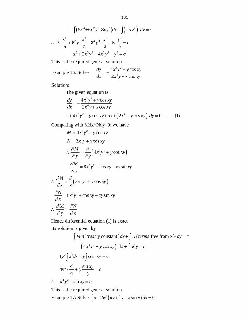
131

4 2 2 3 4 5x +6x y -8xy 5dx y dy c

5 3 2 52 4 3x x x y

5 6 8 55 3 2 5

y y c

5 3 2 2 3 5 x 2 4x y x y y c


Example 16: Solve 3 2

4

4 cos

2 cos

dy x y y xy

dx x y x xy

Solution:


3 3

4

4 cos

2 cos

dy x y y xy

dx x y x xy

3 2 44 cos 2 cos 0...........(1)x y y xy dx x y xy dy

Comparing with Mdx+Ndy=0; we have

3 24 cosM x y y xy

42 cosN x y x xy

3 24 cosM

x y y xyy y

3 2 8 cos sin

Mx y xy xy xy

y

4N2 cosx y y xy

x x

3 8 cos sinN

x y xy xy xyx

M N

y x



y constant free from xMin treat dx N terms dy c

3 24 cos dx ody cx y y xy

2 3 4 cos xy cy x dx y

42 sin

4y4

x xyy c

y

4 2 x siny xy c


Example 17: Solve 2 sin 0yx e dy y x x dx .

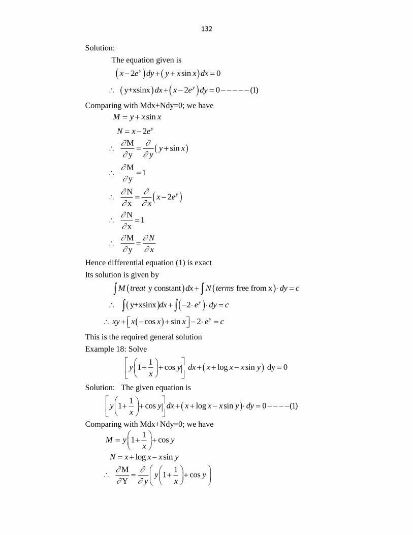
132

Solution:

The equation given is

2 sin 0yx e dy y x x dx

y+xsinx 2 0 (1)ydx x e dy


sinM y x x

2 yN x e

M

siny

y xy

M

1y

N

2x

yx ex

N

1x

M

y

N

x




y+xsinx 2 ydx e dy c

cos sin 2 yxy x x x e c


Example 18: Solve

1

1 cos log sin dy 0y y dx x x x yx


1

1 cos log sin 0 (1)y y dx x x x y dyx


1

1 cosM y yx

log sinN x x x y

M 1

1 cosY

y yy x

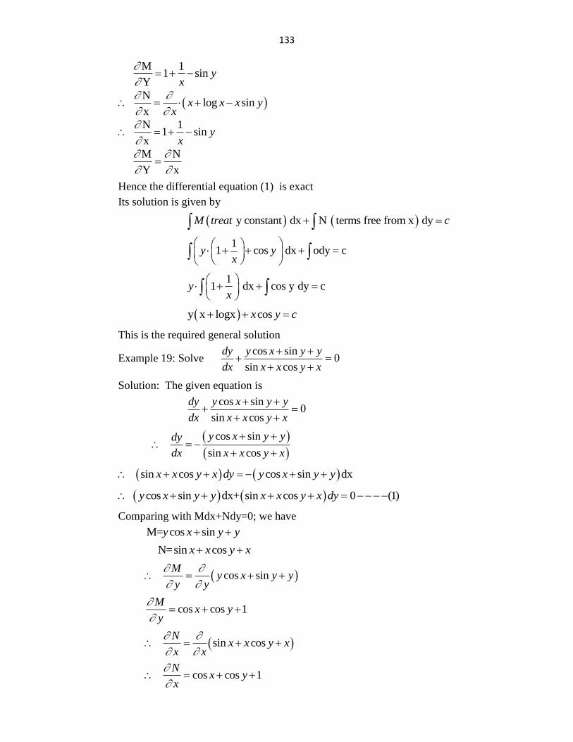
133

M 1 1 sin

Yy

x

N

log sinx

x x x yx

N 1 1 sin

xy

x

M N

Y x

Hence the differential equation (1) is exact


y constant dx N terms free from x dyM treat c

1

1 cos dx ody cy yx

1

1 dx cos y dy cyx

y x logx cosx y c


Example 19: Solve cos sin

0sin cos

dy y x y y

dx x x y x


cos sin

0sin cos

dy y x y y

dx x x y x

cos sin

sin cos

y x y ydy

dx x x y x

sin cos cos sin dxx x y x dy y x y y

cos sin dx+ sin cos 0 (1)y x y y x x y x dy


M= cos siny x y y

N=sin cosx x y x

cos sinM

y x y yy y

cos cos 1M

x yy

sin cosN

x x y xx x

cos cos 1N

x yx

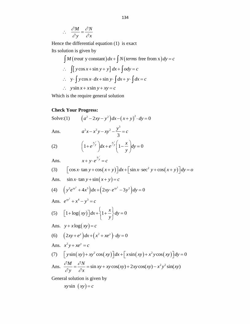
134

M N

y x

Hence the differential equation (1) is exact



cos sin y x y y dx ody c

y cos siny x dx y dx y dx c

sin siny x x y xy c

Which is the require general solution


Solve:(1) 22 22 0a xy y dx x y dy

Ans. 3

2 2 2

3

ya x x y xy c

(2) 1 1 0x x

y y xe dx e dy

y

Ans. x

yx y e c

(3) 2cos tan cos sin sec cosx y x y dx x y x y dy o

Ans. sin tan sinx y x y c

(4) 2 22 3 24 2 3 0xy xyy e x dx xy e y dy

Ans. 2 4 3xye x y c

(5) 1 log 1 0x

xy dx dyy

Ans. logy x xy c

(6) 22 0y yxy e dx x xe dy

Ans. 2 yx y xe c

(7) 2 2sin cos sin cos 0y xy xy xy dx x xy x y xy dy

Ans. 2 2sin cos( ) 2 cos( ) sin( )

M Nxy xy xy xy xy x y xy

y x

General solution is given by

sin xy xy c

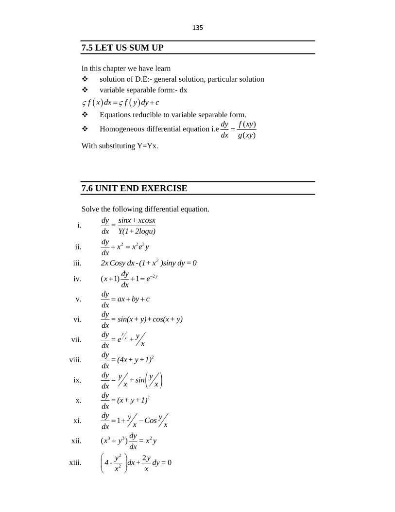
135

7.5 LET US SUM UP


solution of D.E:- general solution, particular solution

variable separable form:- dx

f x dx f y dy c

Equations reducible to variable separable form.

Homogeneous differential equation i.e( )

( )

dy f xy

dx g xy

With substituting Y=Yx.


Solve the following differential equation.

i. dy sinx+ xcosx

=dx Y(1+2logu)

ii. 2 2 3dyx x e y

dx

iii. 22x Cosy dx -(1+ x )siny dy = 0

iv. 2( 1) 1 ydyx e

dx

v. dy

ax by cdx

vi. dy

= sin(x+ y)+cos(x+ y)dx

vii. y

xdy y

= e +xdx

viii. 2dy= (4x+ y+1)

dx

ix. dy y y= +sin

x xdx

x. 2dy= (x+ y+1)

dx

xi. 1dy y y

Cosx xdx

xii. 3 3 2( )dy

x y = x ydx

xiii. 2

2

20

y y4 - dx+ dy =

x x

136

xiv. 2 2

2 2

dy x +3y+ = 0

dx 3x + y

xv. 4( )dy

x y = 3x - 4ydx

*****

8

EQUATION REDUCIBLE TO EXACT

EQUATIONS

UNIT STRUCTURE

8.1 Objective

8.2 Introduction

8.3 Definition

8.4 Linear Equation And Equations Reducible To Linear Form

8.5 Equations reducible to linear form

8.6 Let Us Sum Up

8.7 Check your progress


8.1OBJECTIVE


Find the solution of non-exact .differential equation.

Find the solution of linear .differential equation.

Reducing to non-linear equation into linear equation.

Find the solution of non-linear equation.

8.2 INTRODUCTION

In previous chapter we have learn about exact differential equation & its

solution. Now here we are going to discuss none exact differential

equation. To find the solution of non-exact differential equation we use

integrating factor which convert non-exact differential equation to exact

differential equation. Also we discuss about solution of linear differential

equation.

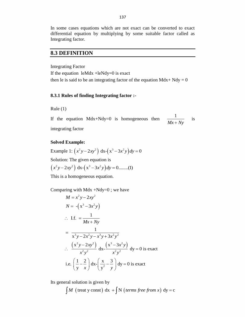
137

In some cases equations which are not exact can be converted to exact

differential equation by multiplying by some suitable factor called as

Integrating factor.

8.3 DEFINITION

Integrating Factor

If the equation leMdx +leNdy=0 is exact

then le is said to be an integrating factor of the equation Mdx+ Ndy = 0

8.3.1 Rules of finding Integrating factor :-

Rule (1)

If the equation Mdx+Ndy=0 is homogeneous then 1

Mx Ny is

integrating factor

Solved Example:

Example 1: 2 2 3 22 dx- x 3 0x y xy x y dy


2 2 3 22 dx- x 3 0........(1)x y xy x y dy

This is a homogeneous equation.

Comparing with Mdx +Ndy=0 ; we have

2 22M x y xy

3 2 - x 3N x y

1

I.f. Mx Ny

3 2 3 2 2

1

x 2 3y x y x y x y

2 2 3 2

2 2 2 2

x 2 x 3 dx- dy 0 is exact

y xy x y

x y x y

2

1 2 x 3i.e. dx- dy 0 is exact

y yx y

Its general solution is given by

treat y const dx N dy c M terms free from x

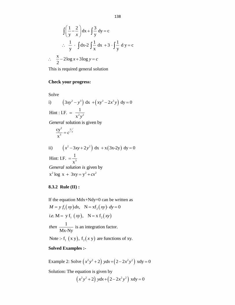
138

1 2 3

dx dy cy yx

1 1 1

dx-2 dx 3 d y cy x y

x 2log 3log

2x y c



Solve

i) 2 3 2 23 dx xy 2 dy 0xy y x y

2 2

1Hint : I.F.

x y

solution is given by General 2

3

cy

x

yxc

ii) 2 23 2 dx x 3x-2y dy 0x xy y

3

1Hint: I.F.

x

given by General solution is 2 2 2x log x 3xy y cx

8.3.2 Rule (II) :

If the equation Mdx+Ndy=0 can be written as

1 2 , N xf 0M y f xy dx xy dy

1 2. . M y f , N x fi e xy xy

1 is an integration factor.Mx-Ny

then

1 2Note :- f x y , f y are functions of xy.x

Solved Examples :-

Example 2: Solve 2 2 2 22 2 2 xdy 0x y ydx x y

Solution: The equation is given by

2 2 2 22 2 2 xdy 0x y ydx x y

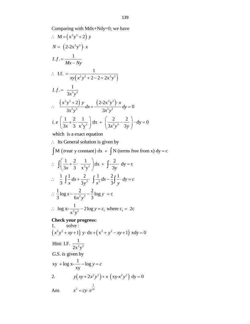
139


2 2 M x y 2 y

2 2 2-2x yN x

1. .I f

Mx Ny

2 2 2 2

1 I.f.

2 2 2x yxy x y

3 3

1. .

3I f

x y

2 2 2 2

3 3 3 3

x y 2 2-2x y 0

3 3

y xdx dy

x y x y

3 2 3 3

1 2 1 2 2. dx dy 0

3 3 x y 3 3i e

x x y y

which is a exact equation

Its General solution is given by

M y constant dx N (terms free from x) dy c treat

3 2

1 2 1 2 dx - dy c

3 3 x y 3yx

2 3

1 1 2 1 2 1

3 3 3dx dx dy c

x y x y

2 2

1 2 2log log c

3 6 3x y

x y

1 12 2

1 log x- 2log where c 2c

x yy c


1. solve :

2 2 2 21 y dx x 1 xdy 0x y xy y xy

2 2

1Hint: I.F.

2x y

. . given by G S is

1xy log x- log

xyy c

2. 2 2 2 22 xydy 0y xy x y x x y

Ans

1

2 xyx cy e

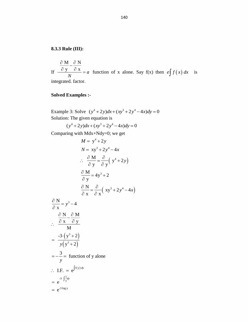
140

8.3.3 Rule (III):

If

M N

y xa

N

function of x alone. Say f(x) then e f x dx is

integrated. factor.

Solved Examples :-

Example 3: Solve 4 3 4( 2 ) ( 2 4 ) 0y y dx xy y x dy


4 3 4( 2 ) ( 2 4 ) 0y y dx xy y x dy

Comparing with Mdx+Ndy=0; we get

4 y 2M y

3 4 xy 2 4N y x

4 M y 2

y yy

3 M

4y 2 y

3 4 N xy 2 4

x xy x

3 N4

xy

N M

x y

M

3

3

-3 y 2

y 2y

3 function of y alone

y

f y

I.F. edy

1-3

y edy

-3 log y e

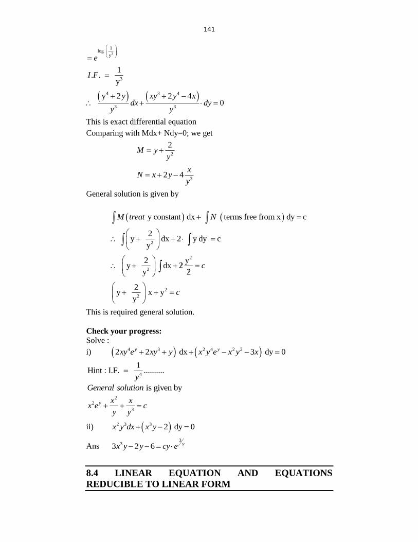
141

3

1log

ye

3

1. .

yI F

4 3 4

3 3

y 2 2 4 0

y xy y xdx dy

y y

This is exact differential equation

Comparing with Mdx+ Ndy=0; we get

2

2M y

y

3

2 4x

N x yy

General solution is given by

y constant dx terms free from x dy c M treat N

2

2 y dx 2 y dy c

y

2

2

2 y y dx 2

y 2c

2

2

2y x y

yc

This is required general solution.


Solve :

i) 4 3 2 4 2 22 2 dx 3 dy 0y yxy e xy y x y e x y x

4

1Hint : I.F. ..........

y

is given by General solution 2

2

3

y x xx e c

y y

ii) 2 3 3 2 dy 0x y dx x y

Ans 3

33 2 6 yx y y cy e

8.4 LINEAR EQUATION AND EQUATIONS

REDUCIBLE TO LINEAR FORM

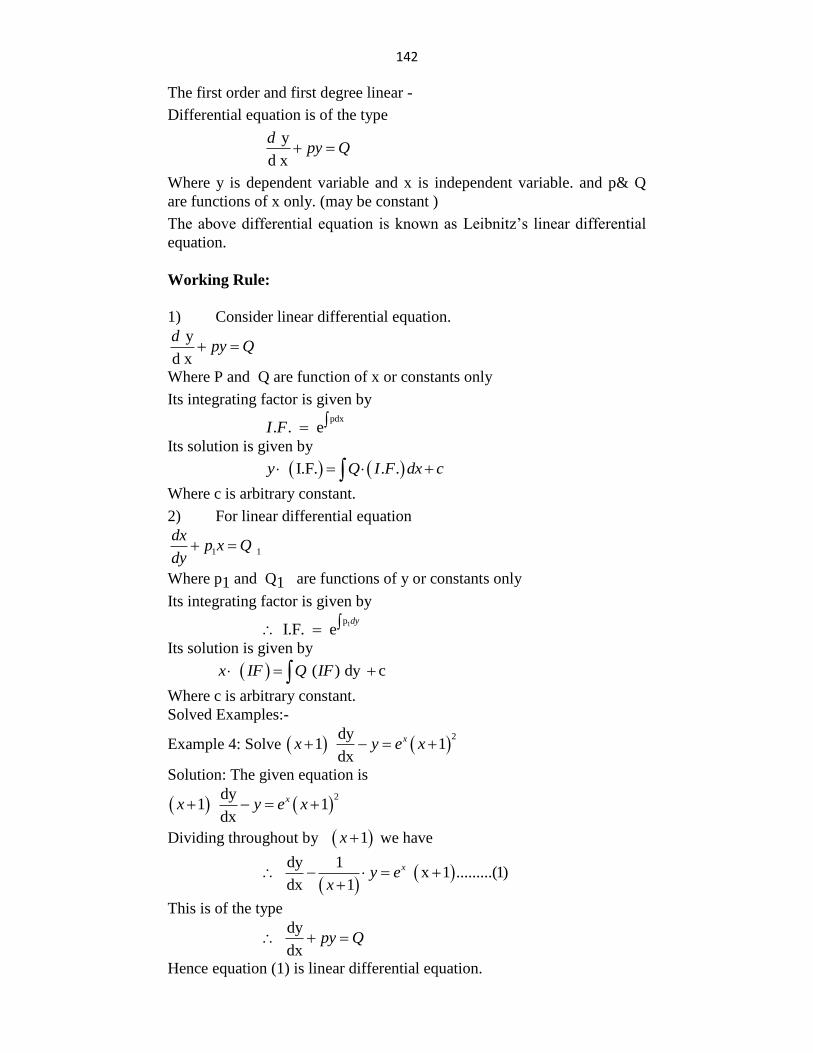
142

The first order and first degree linear -

Differential equation is of the type

y

d x

dpy Q

Where y is dependent variable and x is independent variable. and p& Q

are functions of x only. (may be constant )

The above differential equation is known as Leibnitz‟s linear differential

equation.

Working Rule:

1) Consider linear differential equation.

y

d x

dpy Q

Where P and Q are function of x or constants only

Its integrating factor is given by

pdx

. . eI F


I.F. . .y Q I F dx c

Where c is arbitrary constant.

2) For linear differential equation

1 1 dx

p x Qdy

Where p1 and Q1 are functions of y or constants only

Its integrating factor is given by

1p

I.F. edy


( ) dy cx IF Q IF

Where c is arbitrary constant.

Solved Examples:-

Example 4: Solve 2dy

1 1dx

xx y e x


2dy

1 1dx

xx y e x

Dividing throughout by 1x we have

dy 1

x 1 .........(1)dx 1

xy ex

This is of the type

dy

dx

py Q

Hence equation (1) is linear differential equation.

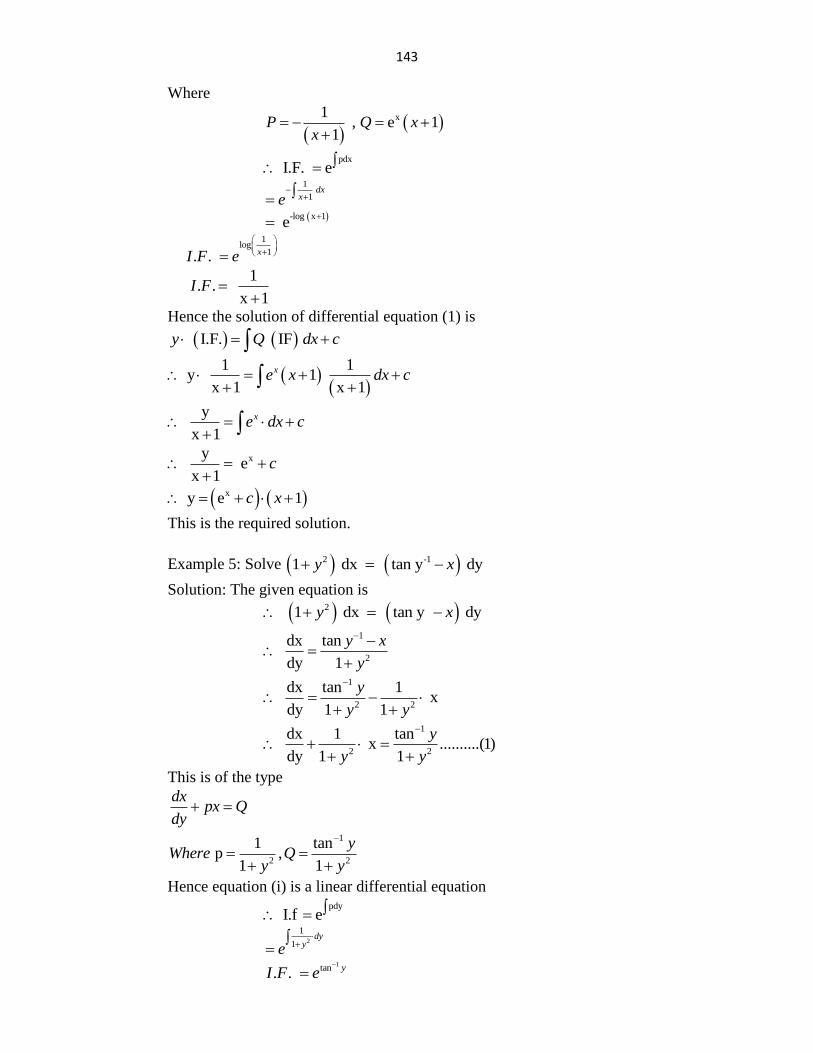
143

Where

x1 , e 1

1P Q x

x

pdx

I.F. e

1

1

dxxe

-log x 1 e

1log

1. . xI F e

1

. . x 1

I F

Hence the solution of differential equation (1) is

I.F. IF y Q dx c

1 1 y 1

x 1 x 1

xe x dx c

y

x 1

xe dx c

xy e

x 1c

x y e 1c x

This is the required solution.

Example 5: Solve 2 -11 dx tan y dyy x


2 1 dx tan y dyy x

1

2

dx tan dy 1

y x

y

1

2 2

dx tan 1 xdy 1 1

y

y y

1

2 2

dx 1 tan x ..........(1)dy 1 1

y

y y

This is of the type

dxpx Q

dy

1

2 2

1 tan p ,

1 1

yWhere Q

y y

Hence equation (i) is a linear differential equation

pdy

I.f e

2

1

1dy

ye

1tan. . yI F e

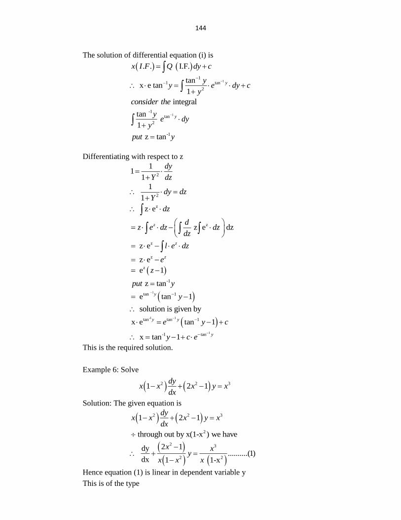
144

The solution of differential equation (i) is

. . I.F.x I F Q dy c

1

11 tan

2

tan x e tan

1

yyy e dy c

y

integral consider the

1

-1tan

2

tan

1

yye dy

y

-1 z tanput y

Differentiating with respect to z

2

11

1

dy

Y dz

2

1 1

dy dzY

z z e dz

z z e dzz d

z e dz dzdz

z z e zl e dz

z z e ze

z e 1z

-1 z tanput y

1tan 1 e tan 1y y

solution is given by

-1 1tan tan 1x e tan 1y ye y c

1-1 tan x tan 1 yy c e


Example 6: Solve

2 2 31 2 1

dyx x x y x

dx


2 2 31 2 1dy

x x x y xdx

2 through out by x(1-x ) we have

2 3

2 2

2 1dy ..........(1)dx 1 1-x

x xy

x x x

Hence equation (1) is linear in dependent variable y

This is of the type

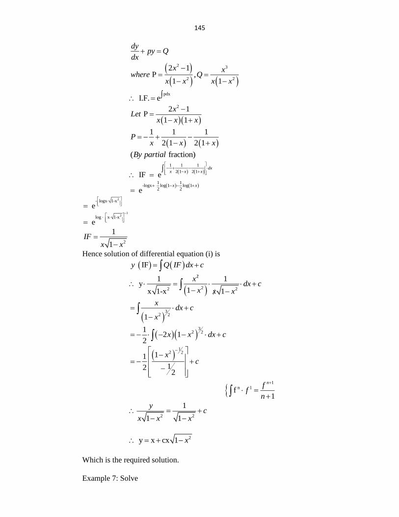
145

dy

py Qdx

2 3

2 2

2 1 P ,

1 1

x xwhere Q

x x x x

pdx

I.F. e

22 1 P

1 1

xLet

x x x

1 1 1

2 1 2 1P

x x x

( fraction)By partial

1 1 1

2 1 2 1 IF e

dxx x x

1 1-logx log 1 log 1

2 2 ex x

2- logx 1-x

e

12log x 1-x

e

2

1

1IF

x x

Hence solution of differential equation (i) is

IFy Q IF dx c

2

22 2

1 1 y

1x 1-x 1

xdx c

x x x

3

2 21

xdx c

x

3

2 212 1

2x x dx c

12 211

122

xc

1

n 1 f1

nff

n

2 2

1

1 1

yc

x x x

2 y x cx 1 x

Which is the required solution.

Example 7: Solve

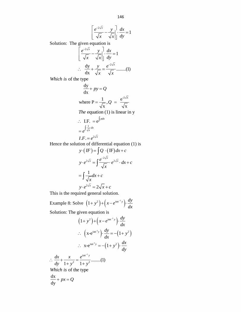
146

2

1xe y dx

dyx x


2

1xe y dx

dyx x

2dy

........(1)dx

xy e

x x

of the type Which is

dy

dx

py Q

-2 x1 e

where P , x x

Q

equation (1) is linear in yThe

I.F. epdx

1dx

xe

2. . xI F e

Hence the solution of differential equation (1) is

IFy IF Q dx c

2

2 2x

x xey e e dx c

x

1

dx cx

2 2xy e x c


Example 8: Solve 12 tan1 y dy

y x edx


12 tan1 y dy

y x edx

-1tan 2 x-e 1y dy

ydx

-1tan 2 x-e 1y dx

ydy

1tan

2 2........(1)

1 1

ydx x e

dy y y

of the type Which is

dx

dypx Q

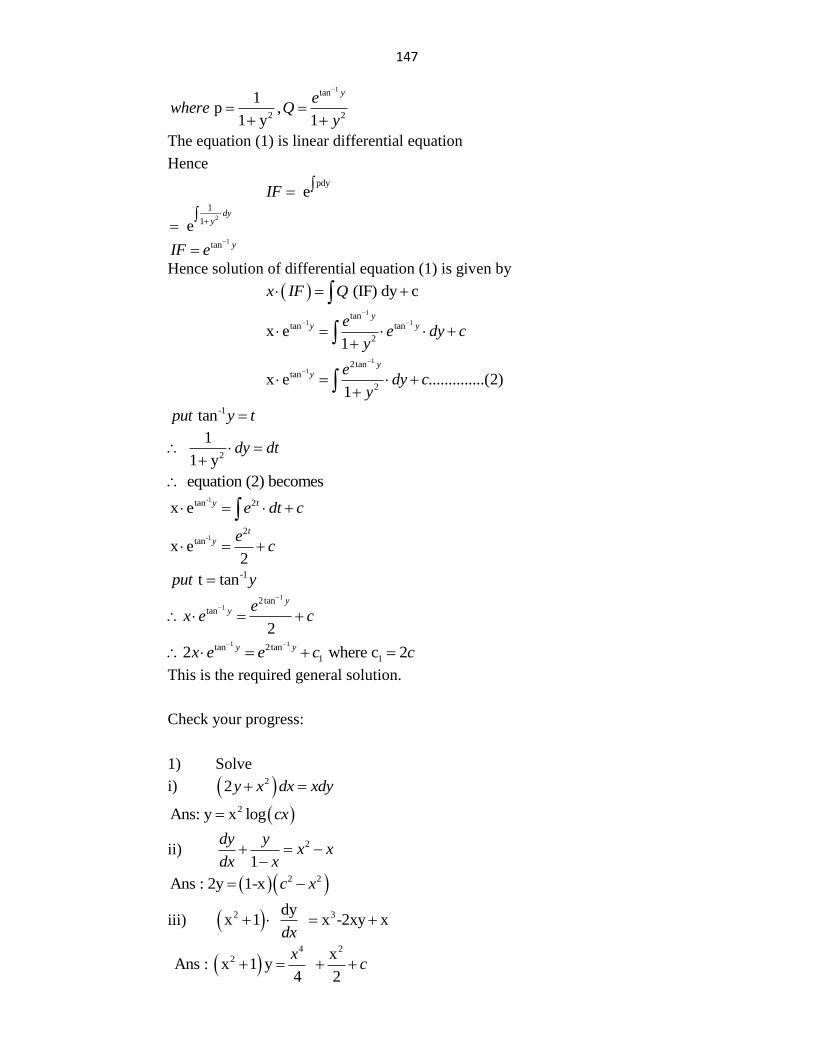
147

1tan

2 2

1 p ,

1 y 1

yewhere Q

y

The equation (1) is linear differential equation

Hence

pdy

eIF

2

1

1 edy

y

1tan yIF e

Hence solution of differential equation (1) is given by

(IF) dy cx IF Q

1

1 1tan

tan tan

2x e

1

yy ye

e dy cy

1

12tan

tan

2x e ..............(2)

1

yy e

dy cy

-1 tanput y t

2

1 1 y

dy dt

equation (2) becomes -1tan 2x e y te dt c

-12

tanx e2

ty e

c

-1 t tanput y 1

12tan

tan

2

yy e

x e c

1 1tan 2tan

1 12 where c 2y yx e e c c



1) Solve

i) 22 y x dx xdy

2Ans: y x log cx

ii) 2 1

dy yx x

dx x

2 2Ans : 2y 1-x c x

iii) 2 3dyx 1 x -2xy x

dx

4 2

2 x Ans : x 1 y

4 2

xc

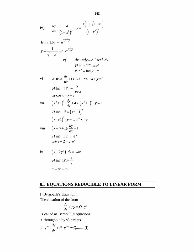
148

iv)

2

3 222 2

1 1

11

x xdy xy

dx xx

2

1-

1int I.F. e xH

2

1

1

2

1

1

xy c cx

v) 2secydx xdy e dy

yint : I.F. eH

tanyx e y c

vi cos cos sin 1dy

x x x x x ydx

x

int : I.F. sec

Hx

cosxy x x c

vii 3 2

2 21 4 1 1dy

x x x ydx

2

2int : If x 1H

2

2 11 tanx y x c

viii 1 1dy

x ydx

-yint : I.F. eH

2 yx y c e

ix 32x y dy ydx

1

int I.F.y

H

3x y cy

8.5 EQUATIONS REDUCIBLE TO LINEAR FORM

I) Bernoulli‟s Equation :

The equation of the form

ndy

py Q ydx

called as Bernoulli's equationsis n throughout by y , we get

1 y .........(1)n ndyP y Q

dx

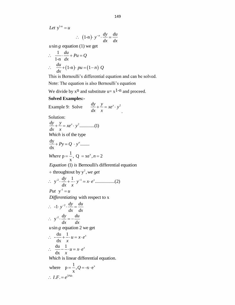
149

1-n yLet u

1-n n dy duy

dx dx

sin equation (1) we getu g

1 1-n

duPu Q

dx

1-n 1 du

pu n Qdx

This is Bernoulli‟s differential equation and can be solved.

Note: The equation is also Bernoulli‟s equation

We divide by xn and substitute u= x1-n and proceed.

Solved Examples:-

Example 9: Solve 2xdy y

xe ydx x

.

Solution:

2.............(1) xdy yxe y

dx x

is of the type Which

dy ........

dx

nPy Q y

x1 p , Q xe , 2

xWhere n

(1) Bernoulli's differential equation Equation is 2 throughtout by y , we get

-2 11 y .................(2)xdy

y x edx x

-1 yPut u

with respect to xDifferentiating

2 -1dy du

ydx dx

-2 ydy du

dx dx

sin equation 2 we get u g

du 1 -

dx

xu x ex

du 1 dx

xu x ex

is linear differential equation. Which

x1where p , -x e

xQ

. . PdxI F e

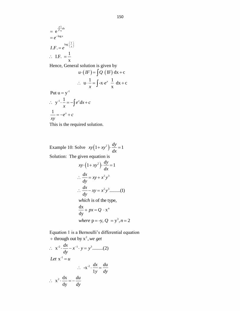
150

1-

x edx

log xe

1log

. . xI F e

1 I.F.

x

Hence, General solution is given by

IF dx cu IF Q

1 1

u -x dx cx

xex

-1Put u y

-1 1 y xe dx c

x

1 xe cxy


Example 10: Solve 21 1dy

xy xydx


21 1dy

xy xydx

2 3dx

xy x ydy

2 3.........(1)

dxxy x y

dy

is of the type,which

ndx

xdy

px Q

3 p -y, y , 2where Q n

Equation 1 is a Bernoulli‟s differential equation 2 through out by x , we get

-2 1 3 x .........(2)dx

x y ydy

-1 xLet u

-2 -x

1

dx du

y dy

2 dx x

dy

du

dy

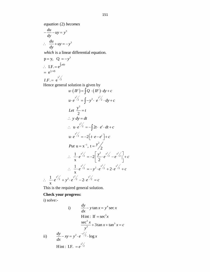
151

(2) equation becomes

3duuy y

dy

3 du

uy ydy

is a linear differential equation.which 3p y, Q y

I.F. epdy

y e y d 2y

2. . eI F

Hence general solution is given by

u IF Q IF dy c

2 2

32 2 y y

u e y e dy c

2y

2

Let t

y dy dt

2

2 u 2 y

te t e dt c

2

2u 2y

te t e e c

2

1 u x , t2

yPut

2 2 22

2 2 21

2x 2

y y yye e e c

2 2 2

22 2 21

2x

y y y

e y e e c

2 2 2

22 2 21

2x

y y y

e y e e c



i) solve:-

i) 4tan sec

dyy x y x

dx

3Hint : If sec x

3

3

3

sec3tan tan

xx x c

y

ii) 2

2 2 logxdy

xy y e xdx

2

2Hint : I.F. x

e

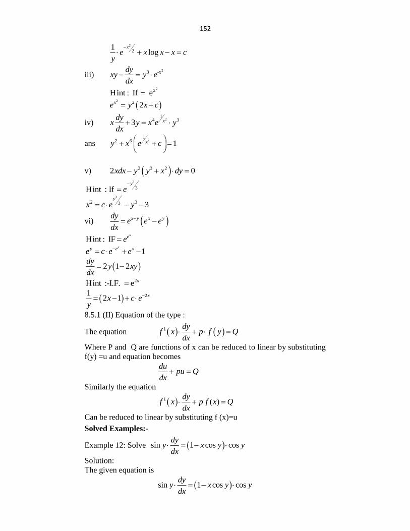
152

2

21

logx

e x x x cy

iii) 23 -xdy

xy y edx

2xHint : If e

2 2 2xe y x c

iv) 2

14 33 x

dyx y x e y

dx

ans 2

12 6 1xy x e c

v) 2 3 22 0xdx y y x dy

3

3Hint : Ify

e

3

2 33 3y

x c e y

vi) x y x ydye e e

dx

Hint : IFxee

1xy e xe c e e

2 1 2dy

y xydx

2xHint :-I.F. e

212 1 xx c e

y

8.5.1 (II) Equation of the type :

The equation 1 dyf x p f y Q

dx

Where P and Q are functions of x can be reduced to linear by substituting

f(y) =u and equation becomes

du

pu Qdx

Similarly the equation

1 ( )dy

f x p f x Qdx

Can be reduced to linear by substituting f (x)=u

Solved Examples:-

Example 12: Solve sin 1 cos cosdy

y x y ydx

Solution:


sin 1 cos cosdy

y x y ydx

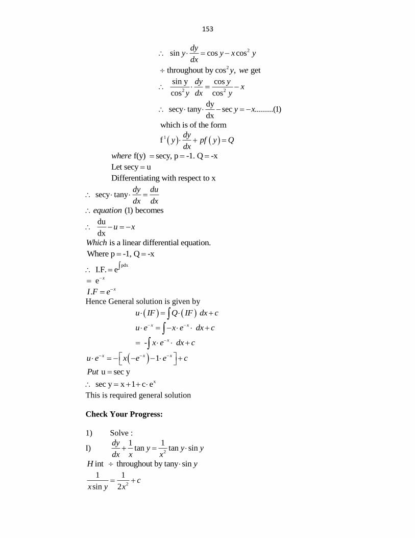
153

2 sin cos cos

dyy y x y

dx

2 throughout by cos , gety we

2 2

sin y cos cos cos

dy yx

y dx y

dy

secy tany sec .........(1)dx

y x

which is of the form

1fdy

y pf y Qdx

f(y) secy, p -1. Q -xwhere

Let secy u

Differentiating with respect to x

secy tanydy du

dx dx

(1) becomes equation

du dx

u x

is a linear differential equation.Which

Where p -1, Q -x

pdx

I.F. e

e x

. xI F e

Hence General solution is given by

u IF Q IF dx c

x xu e x e dx c

- xx e dx c

1x x xu e x e e c

u sec yPut x sec y x 1 c e



1) Solve :

I) 2

1 1tan tan sin

dyy y y

dx x x

int throughout by tany sinH y

2

1 1

sin 2c

x y x

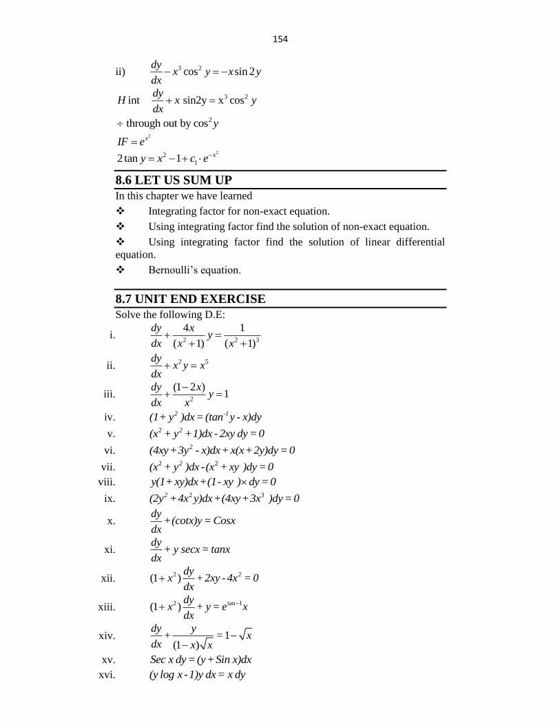
154

ii) 3 2cos sin 2dy

x y x ydx

3 2int sin2y x cosdy

H x ydx

2 through out by cos y 2xIF e

22

12tan 1 xy x c e

8.6 LET US SUM UP

In this chapter we have learned

Integrating factor for non-exact equation.

Using integrating factor find the solution of non-exact equation.

Using integrating factor find the solution of linear differential

equation.

Bernoulli‟s equation.


Solve the following D.E:

i. 2 2 3

4 1

( 1) ( 1)

dy xy

dx x x

ii. 2 5dyx y x

dx

iii. 2

(1 2 )1

dy xy

dx x

iv. 2 -1(1+ y )dx=(tan y - x)dy

v. 2 2(x + y +1)dx - 2xy dy = 0

vi. 2(4xy+3y - x)dx+ x(x+2y)dy = 0

vii. 2 22(x + y )dx -(x + xy )dy = 0

viii. y(1+ xy)dx+(1- xy ) dy =0

ix. 2 32(2y +4x y)dx+(4xy+3x )dy = 0

x. dy

+(cotx)y = Cosxdx

xi. dy

+ y secx = tanxdx

xii. 2 2(1 )dy

x +2xy - 4x = 0dx

xiii. 2 tan 1(1 )dy

x + y = e xdx

xiv. 1(1 )

dy y+ = x

dx x x

xv. Sec x dy =(y+Sin x)dx

xvi. (y log x -1)y dx= x dy

155

xvii. 3 3dy+ xy = x y

dx

xviii. 2

121

dy xy+ = xy

dx x

xix. 2dyy -Cosx = y (1- Sinx)Cosx

dx

xx. 2 2y dx+ x(1- 3x y )dy = 0

*****

9

APPLICATIONS OF DIFFERENTIAL

EQUATIONS

UNIT STRUCTURE

9.1 Objective

9.2 Introduction

9.3 Geometrical

9.4 Physical Application

9.5 Simple Electric Circuits

9.6 Newton‟s Law of Cooling

9.7 Let Us Sum Up


9.1 OBJECTIVE


Use differential equation to find the equation of any curve.

Use differential equation physics like projectile motion, S.H.M‟s,

Rectilinear motion, Newton‟s law of cooling.

Use differential equation in electric circuits.

9.2 INTRODUCTION

In previous chapter we have learn to solve differential equations.

We differ type. Now here we are going use differential equation in

different field its useful to geometrical, physical, and electronic circuits,

civil engineering and so on we are going to discuss few application of

differential equation.

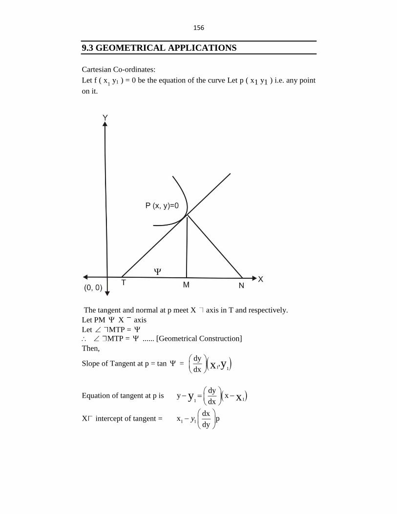
156

9.3 GEOMETRICAL APPLICATIONS

Cartesian Co-ordinates:

Let f ( x1 y1 ) = 0 be the equation of the curve Let p ( x1 y1 ) i.e. any point

on it.

The tangent and normal at p meet X axis in T and respectively.

Let PM X axis

Let MTP =

MTP = ...... [Geometrical Construction]

Then,

Slope of Tangent at p = tan = 1 1

dy,

dxyx

Equation of tangent at p is 11

dyy x

dxy x

X intercept of tangent = 1 1

dxx p

dyy

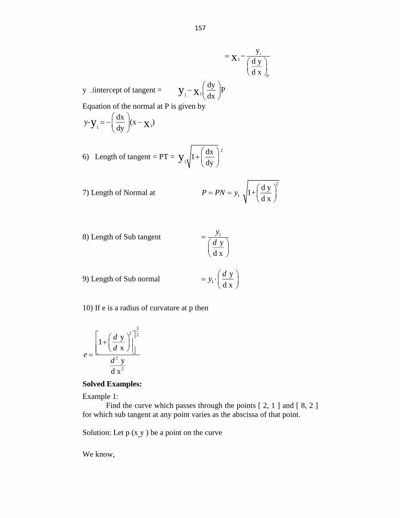
157

1

1

p

y

d y

d x

x

y intercept of tangent = 11

dyP

dxy x

Equation of the normal at P is given by

11

dxy- (x )

dyy x

6) Length of tangent = PT = 2

1

dx1

dyy

7) Length of Normal at

2

1

d y 1+

d xP PN y

8) Length of Sub tangent 1

y

d x

y

d

9) Length of Sub normal 1

y

d x

dy

10) If e is a radius of curvature at p then

32 2

2

2

y1

x

y

d x

d

de

d

Solved Examples:

Example 1:

Find the curve which passes through the points [ 2, 1 ] and [ 8, 2 ]

for which sub tangent at any point varies as the abscissa of that point.

Solution: Let p (x,y ) be a point on the curve

We know,

158

y

subtangentdy

dx

From given condition-

y

xdy

dx

y

kx.....[k constant]dy

dx

dy

y kxdx

1 k

dx dyx y

dy 1

k dxy x

which is in variable seperate form

integrate both side

1

k. dy constanty

k. log y =log x + log c

k

log =log cxy

k

cx ....... 1y

The Curve passes through the points [2,1] and [6, 2]

put x = 2 , y = 1, in equation [1]

k

21 c

1 2c

1

c2

put x = 8, y = 2, in eqn [1]

k

c x 82

4k 1

x 2

82

k

42

k 2

2 2

K 2

put Value of C and K in eqn [1]

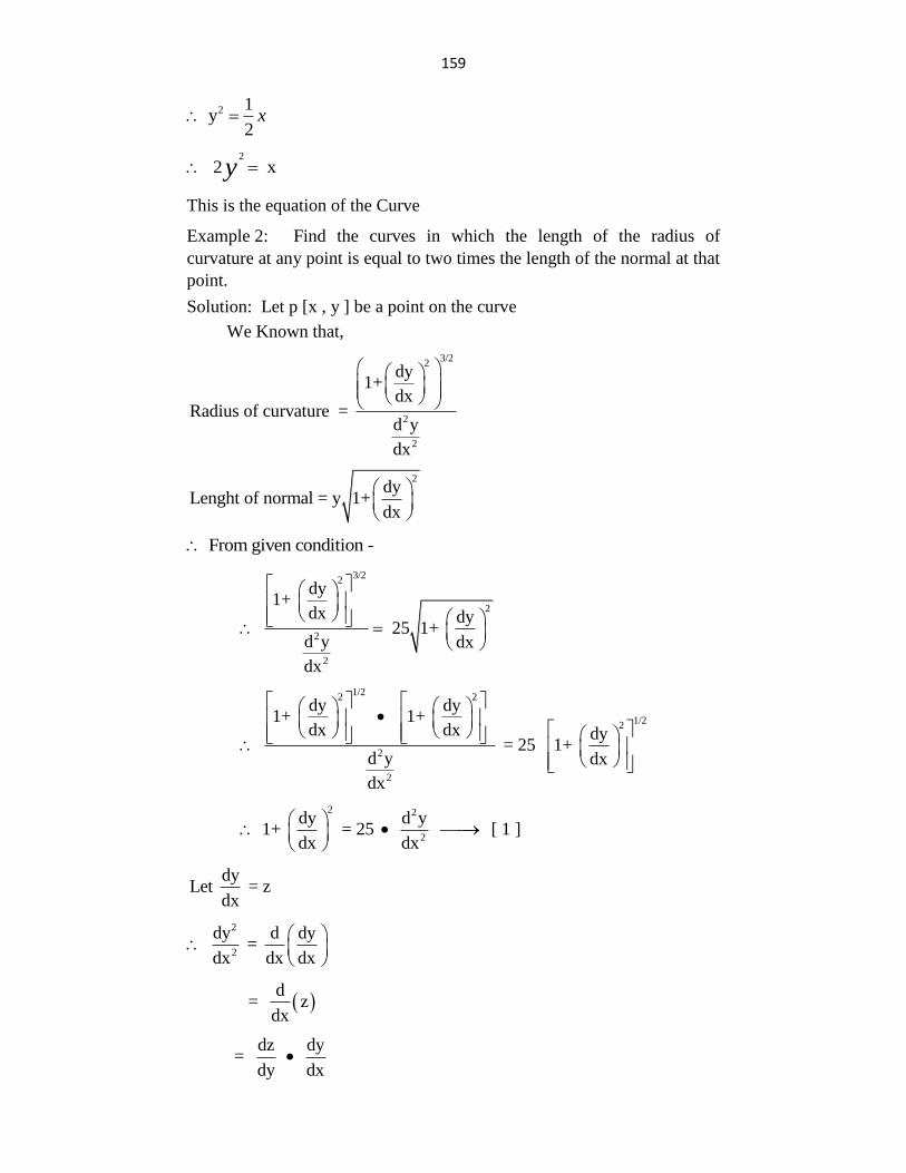
159

2 1 y

2x

2

2 xy

This is the equation of the Curve

Example 2: Find the curves in which the length of the radius of

curvature at any point is equal to two times the length of the normal at that

point.

Solution: Let p [x , y ] be a point on the curve

We Known that,

3/22

2

2

dy1+

dxRadius of curvature =

d y

dx

2dy

Lenght of normal = y 1+dx

From given condition -

3/22

2

2

2

dy1+

dx dy 25 1+

d y dx

dx

1/22 2

1/22

2

2

dy dy1+ 1+

dx dx dy = 25 1+

d y dx

dx

2 2

2

dy d y 1+ = 25 [ 1 ]

dx dx

dyLet = z

dx

2

2

dy d dy = dx dx dx

d

= zdx

dz dy =

dy dx

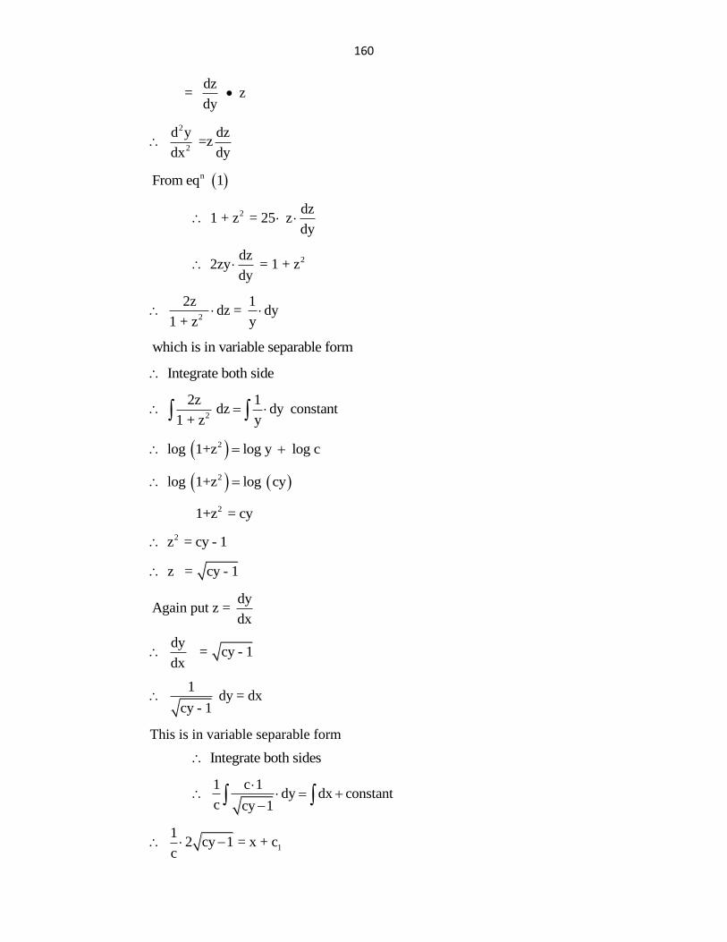
160

dz = z

dy

2

2

d y dz =zdx dy

nFrom eq 1

2 dz 1 + z = 25 z

dy

2dz 2zy = 1 + z

dy

2

2z 1 dz = dy1 + z y

which is in variable separable form

Integrate both side

2

2z 1 dz dy constant

1 + z y

2 log 1+z log y log c

2 log 1+z log cy

2 1+z = cy

2 z = cy - 1

z = cy - 1

dyAgain put z =

dx

dy = cy - 1dx

1 dy = dx

cy - 1


Integrate both sides

1 c 1

dy dx constantc cy 1

1

1 2 cy 1 = x + cc

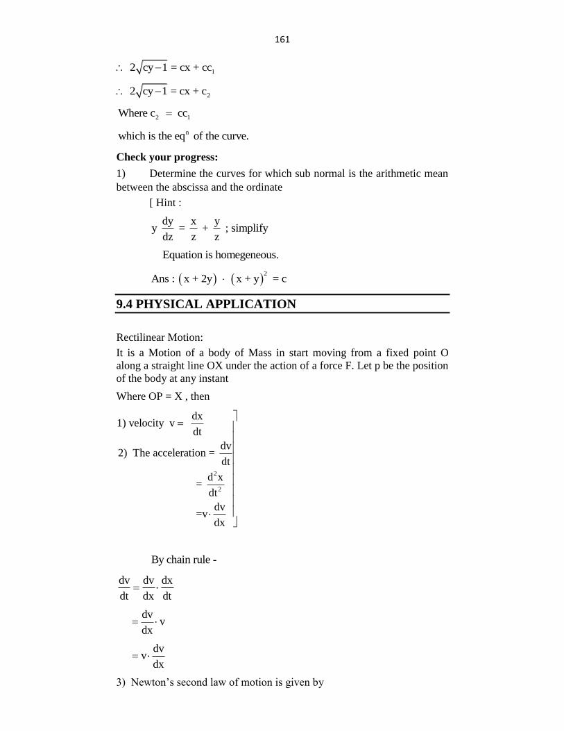
161

1 2 cy 1 = cx + cc

2 2 cy 1 = cx + c

2 1Where c cc

nwhich is the eq of the curve.


1) Determine the curves for which sub normal is the arithmetic mean

between the abscissa and the ordinate

[ Hint :

dy x y

y = + ; simplifydz z z

Equation is homegeneous.

2

Ans : x + 2y x + y = c

9.4 PHYSICAL APPLICATION

Rectilinear Motion:

It is a Motion of a body of Mass in start moving from a fixed point O

along a straight line OX under the action of a force F. Let p be the position

of the body at any instant

Where OP = X , then

2

2

dx1) velocity v

dt

dv2) The acceleration =

dt

d x =

dt

dv =v

dx

By chain rule -

dv dv dx

dt dx dt

dv v

dx

dv v

dx

3) Newton‟s second law of motion is given by

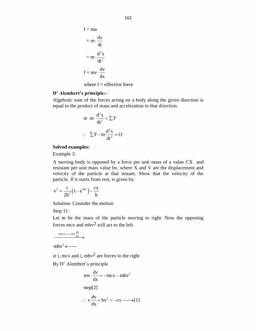
162

f = ma

dv

= mdt

2

2

d x = m

dt

dv

f = mvdx

where f = effective force

D’ Alembert’s principle:-

Algebraic sum of the forces acting on a body along the given direction is

equal to the product of mass and acceleration in that direction.

2

2

d xie m F

dt

2

2

d x F - m O

dt

Solved examples:

Example 3:

A moving body is opposed by a force per unit mass of a value CX and

resistant per unit mass value bv, where X and V are the displacement and

velocity of the particle at that instant. Show that the velocity of the

particle. If it starts from rest, is given by.

2 2bx

2

c cxv 1 e

2b b

Solution: Consider the motion

Step 1) :

Let m be the mass of the particle moving to right. Now the opposing

forces mcx and mbv2 will act to the left.

dvmcx mv

dx

2mbv

ie mcx and mbv2 are forces to the right

By D‟ Alembert‟s principle

2dv

mv mcx mbvdx

step[2]

2dv

v bv cx [1]dx

163

2Let v z

dv dz

2vdx dx

neq [1] becomes

1 dz

bz cx2 dx

dz

2bz 2cxdx

which is a linear equation in z

p = 2b. Q = -2cx.

pdx

2bdx

I.F. = e

= e

2bx

I.F. = e

Its general solution is given by

z [ IF ] = IF dx constantQ

2bx 2bx

1z -2cx dx ce e

2bx

1 -2c x dx ce

2bx 2bx

1

d -2c x dx- x dx c

dne e

2bx 2bx

1 -2c x 1 c2 2

e e dxb b

2bx 2bx

2bx

1

x 1z = 2c +

2b 2b 2b

e ee c

2bx

2 2bx 2bx

2 1

-cx c +

b 2b

ev e e c

2 -2bx

2 1

cx c = [3]

b 2bv c e

1

[III] to find , we impose initial conditionsc

nie for x = o , v = o in eq [3]

164

12

c o = 0 + + c

2b

21

c = -

2bg

n

1put values of in eq [3]g

2 2

2 2

cx c c v = +

b 2b 2b

bxe

2 2

2

c cx v = 1

2b b

bxe

Example 4: A body of mass m. Falling from rest, is subject to the force

of gravity and an air resistance proportional to the square of the velocity

[ie kv2 ]. If it falls through a distance x and possesses a velocity v at that

instant show that

22

2 2

2k x alog , where mg = ka

m a v

Solution:

Step

Let the body of mass m fall from „O‟

The forces acting on the body are

1) Its weight mg acting vertically downwards.

2) The resistance kv2 of the air acting vertically upwards.

The net forces acting on the body vertically downwards

= mg kv2 . . . . [ mg ka2 given]

= ka2 kv2

= k [ a2 v2 ] . . . . . .[ 1 ]

Step [ 2 ] By D‟Alembert‟s Principle

2 2 k a vdv

mvdx

2 2

v k a v m

dv dx


Integrating both sides

1 12 2

1 2 . . . constant

2

v kdv dx c c

a v m

2 2

1

1 log 2

2

ka v x c

m

165

Step [ 3 ] To Final c1 , we put initial conditions

ie when x = o , v = o.

From 2

2

1

1 log a

2c

put value of c1 in eqn [ 2 ]

2 2 21 1 log a v log a

2 2

kx

m

2 2 21 1 log a v log a

2 2

kx

m

2 2 22 log a v log a

kx

m

2 2 2 2 log a log a v

kx

m

2

2 2

2 a log

a v

kx

m


1) A particle of Unit mass is projected upward with velocity u and the

resistance of air produces a retardation kv2 and v is the velocity at any

instant show that the velocity v with which the particle will return to the

point of projection is given by

2 2

1 1 =

u

k

v g

2) Determine the least velocity with which a particle must be

projected vertically upwards so that it does not return to the Earth. Assume

that it is acted upon by the gravitational attraction of the earth only.

Ans : Least Velocity 2vo gR

Radius of earthR

3) A paratrooper and his parachute weigh 50 kg. At the instant

parachute opens. He is Travelling vertically downward at the speed of 20

m/s. If the Air resistance varies directly as the instantaneous velocity and

its 20 Newtons. When the velocity is 10 m/s Find the limiting velocity, the

position and the velocity of the paratrooper at any time “t”.

-gt/255 s . . . = 25 m/sev

-gt/25

1

25x =5 st+

ge c

-gt/25125 =25t 1 ex

g

166

9.5 SIMPLE ELECTRIC CIRCUITS

The following Notations are frequently used. Units are given in Brackets .

secondst Time

q coulombs arg Ch e on capacitor

i ampere Current

e volts voltage

R ohms Re tansis ce

L Hentries tanIndua ce

C Farads tancapaci ce

Current is the rate of electricity

dq i =

dt

[ II ] Current at each point of a network is got from Kirchhoff‟s laws :

1) The algebraic sum of the currents into any point is zero.

2) Around any closed path the algebraic sum of the voltage drops in

any specific direction is zero.

3) Voltage drops as current i flows through a resistance R is Ri ;

through an induction L is di

Ldt

and through a capacitor C is q

c.

Solved examples:

Example 5: A constant emf E volts is applied to a ckt. containing a

constant resistance. R ohms in

series and a constant inductance L henries. It the initial current is zero,

show that the current builds upto half its theoretical maximum

in log 2L

R seconds.

Solution:

Step (1) R

Let i be the current in the circuit at any time „t‟ .

The by Kirchoff‟s law, we have

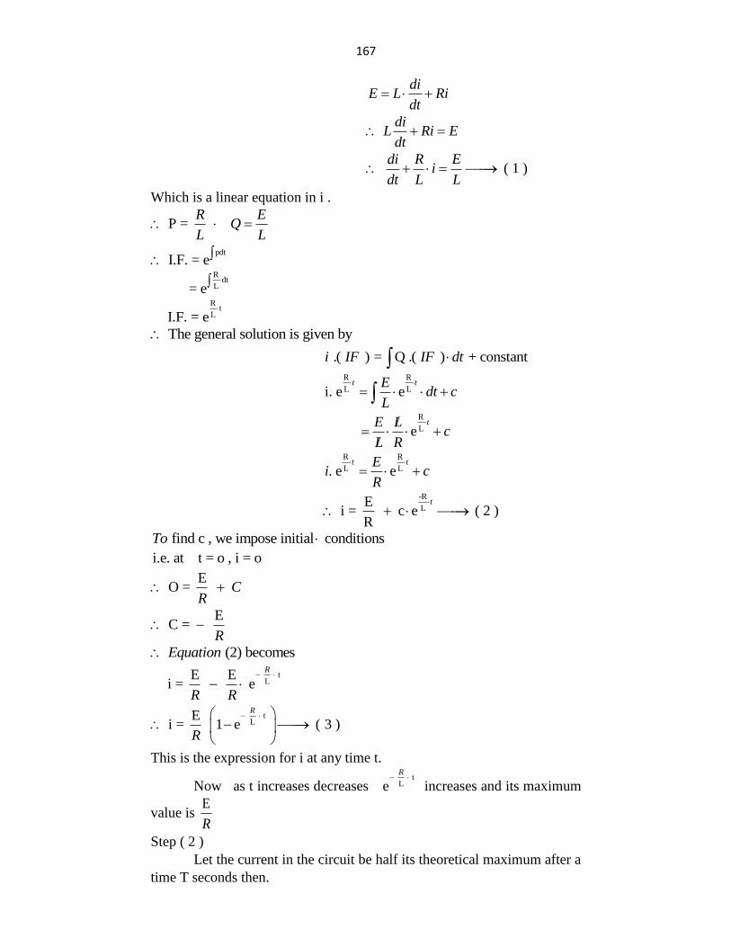
167

di

E L Ridt

di

L Ri Edt

( 1 )di R E

idt L L

Which is a linear equation in i .

P = R E

QL L

pdt

I.F. = e R

dtL = e

R

tL I.F. = e

The general solution is given by

.( ) = Q .( ) + constanti IF IF dt

R R

L Li. e et tE

dt cL

R

L etE L

cL R

R R

L L. e et tE

i cR

-R

LE

i = c e ( 2 )R

t

find c , we impose initial conditionsTo

i.e. at t = o , i = o

E O = C

R

E C =

R

(2) becomesEquation

tL

E E i = e

R

R R

tL

E i = 1 e ( 3 )

R

R

This is the expression for i at any time t.

Now as t increases decreases tLeR

increases and its maximum

value is E

R

Step ( 2 )

Let the current in the circuit be half its theoretical maximum after a

time T seconds then.

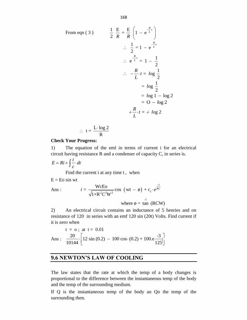
168

From eqn ( 3 ) 1 E E

= 1 e2

Rt

L

R R

1

= 1 e2

Rt

L

1

e = 1 2

Rt

L

1

= og 2

Rt l

L

1

= og 2

l

= og 1 log 2 l

= O og 2l

= og 2R

t lL

L log 2

t = R


1) The equation of the eml in terms of current i for an electrical

circuit having resistance R and a condenser of capacity C, in series is.

iE Ri dt

c

Find the current i at any time t , when

E = Eo sin wt

Ans : 12 2 2

WcEo = cos wt o + c

1+R

t

RCi eC W

-1

where o = tan (RCW)

2) An electrical circuit contains an inductance of 5 henries and on

resistance of 120 in series with an emf 120 sin (20t) Volts. Find current if

it is zero when

t = o ; at t = 0.01

Ans : 20 -3

12 sin (0.2) 100 cos (0.2) + 100.e10144 125

9.6 NEWTON’S LAW OF COOLING

The law states that the rate at which the temp of a body changes is

proportional to the difference between the instantaneous temp of the body

and the temp of the surrounding medium.

If Q is the instantaneous temp of the body an Qo the temp of the

surrounding then.

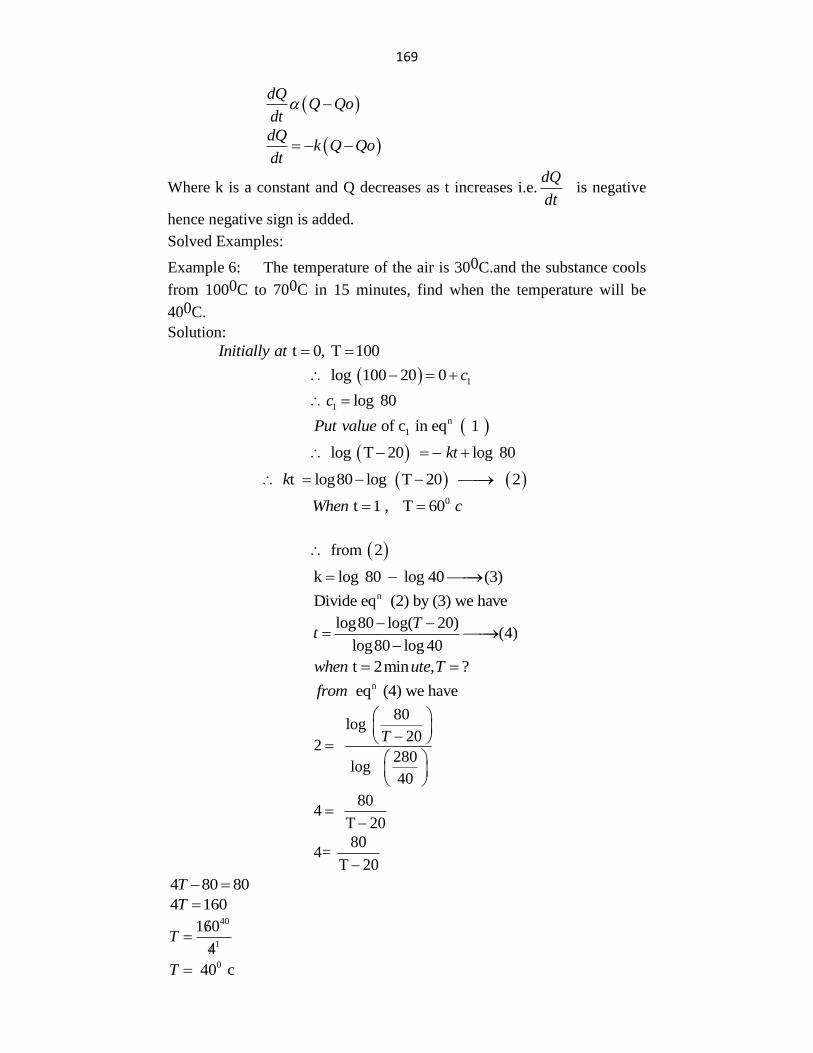
169

dQ

Q Qodt

dQ

k Q Qodt

Where k is a constant and Q decreases as t increases i.e.dQ

dt is negative

hence negative sign is added.

Solved Examples:

Example 6: The temperature of the air is 300C.and the substance cools

from 1000C to 700C in 15 minutes, find when the temperature will be

400C.

Solution:

t 0, T 100Initially at

1 log 100 20 0 c

1 log 80c

n

1 of c in eq 1 Put value

log T 20 log 80kt

t log80 log T 20 2k

0 t 1 , T 60When c

from 2

k log 80 log 40 (3)

n Divide eq (2) by (3) we have

log80 log( 20)

(4)log80 log 40

Tt

t 2min , ?when ute T

n eq (4) we have from

80log

202

280log

40

T

80

4 T 20

80

4= T 20

4 80 80T

4 160T 40

1

160

4T

0 40 cT

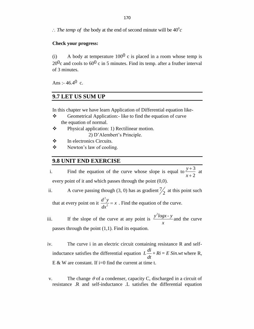
170

0 the body at the end of second minute will be 40The temp of c


(i) A body at temperature 1000 c is placed in a room whose temp is

200c and cools to 600 c in 5 minutes. Find its temp. after a fruther interval

of 3 minutes.

Ans :- 46.40 c.

9.7 LET US SUM UP

In this chapter we have learn Application of Differential equation like-

Geometrical Application:- like to find the equation of curve

the equation of normal.

Physical application: 1) Rectilinear motion.

2) D‟Alembert‟s Principle.

In electronics Circuits.

Newton‟s law of cooling.


i. Find the equation of the curve whose slope is equal to3

2

y

x

at

every point of it and which passes through the point (0,0).

ii. A curve passing though (3, 0) has as gradient 72

at this point such

that at every point on it 2

2

d yx

dx . Find the equation of the curve.

iii. If the slope of the curve at any point is 2y logx - y

xand the curve

passes through the point (1,1). Find its equation.

iv. The curve i in an electric circuit containing resistance R and self-

inductance satisfies the differential equation di

L + Ri = E Sin.wtdt

where R,

E & W are constant. If i=0 find the current at time t.

v. The change of a condenser, capacity C, discharged in a circuit of

resistance .R and self-inductance .L satisfies the differential equation

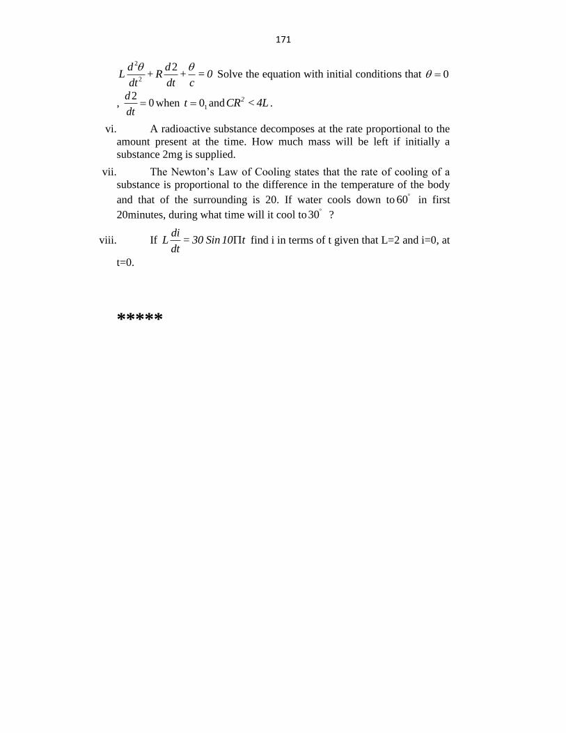
171

2

2

2d dL + R + = 0

dt dt c

Solve the equation with initial conditions that 0

,

20

d

dt when 10t and

2CR < 4L .

vi. A radioactive substance decomposes at the rate proportional to the

amount present at the time. How much mass will be left if initially a

substance 2mg is supplied.

vii. The Newton‟s Law of Cooling states that the rate of cooling of a

substance is proportional to the difference in the temperature of the body

and that of the surrounding is 20. If water cools down to 60 in first

20minutes, during what time will it cool to30 ?

viii. If di

L = 30 Sin 10 tdt

find i in terms of t given that L=2 and i=0, at

t=0.

*****

172

10

SUCCESSIVE DIFFERENTIATION

UNIT STRUCTURE

10.1 Objective

10.2 Introduction

10.3 Some standard results

10.4 Type III: Using Complex Numbers

10.5 Problems

10.6 Let Us Sum Up


10.1 OBJECTIVE


Find higher order derivative

Formula of nth order derivative

Leibnitz‟s theorem

Application of Leibnitz‟s theorem

10.2 INTRODUCTION

In this chapter we shall study the methods of finding higher

ordered derivatives for a given functional expression.

This is done in two stages:

Stage I : We shall establish some standard results and solve some

problems using these results.

Stage II : We shall prove Leibnitz theorem and using it find higher order

derivatives of given function

Notation:- Different notations used for derivatives of y=f(x) with respect

to x are

2

2, ,....... ,....... (Due to Lebinitz)

n

n

dy d y d y

dx dx dx

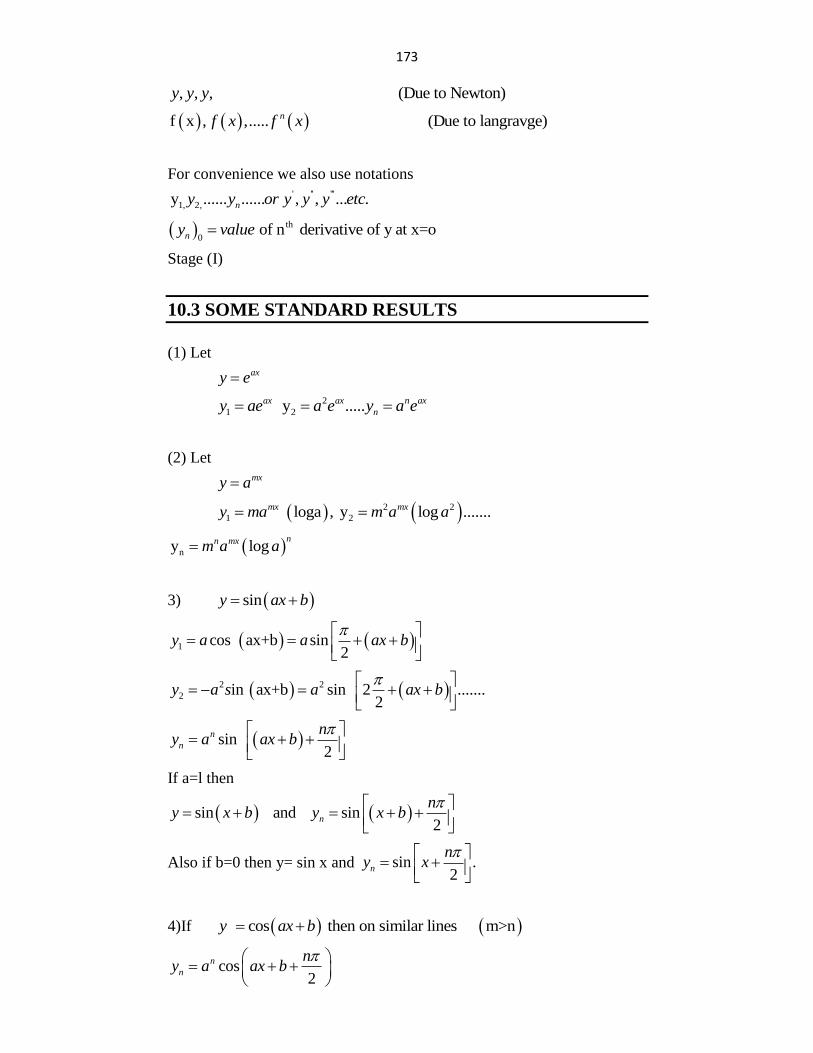
173

, , , (Due to Newton)y y y

f x , ,..... (Due to langravge)nf x f x

For convenience we also use notations ' '' '''

1, 2,y ...... ...... , , ... .ny y or y y y etc

th

0 of n derivative of y at x=ony value

Stage (I)

10.3 SOME STANDARD RESULTS

(1) Let

axy e

2

1 2 y .....ax ax n ax

ny ae a e y a e

(2) Let

mxy a

2 2

1 2 loga , y log .......mx mxy ma m a a

ny lognn mxm a a

3) siny ax b

1 cos ax+b sin2

y a a ax b

2 2

2 in ax+b sin 2 .......2

y a s a ax b

sin 2

n

n

ny a ax b

If a=l then

sin and sin2

n

ny x b y x b

Also if b=0 then y= sin x and sin .2

n

ny x

4)If cos then on similar lines m>ny ax b

cos2

n

n

ny a ax b

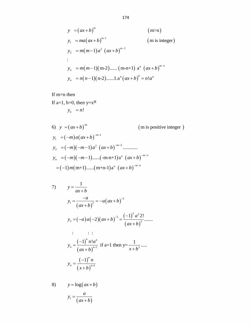
174

m>nm

y ax b

1

1 m is integerm

y ma ax b

22

2 1 m

y m m a ax b

:

. n 1 m-2 ...... m-n+1 a m n

ny m m ax b

0n 1 n-2 ......1.a ! n

ny n n ax b n a

If m=n then

If a=1, b=0, then y=xn

!ny n

6) -m

m is positive integer y ax b

1

1 m

y m a ax b

22

2 1 ............ m

y m m a ax b

n 1 ...... -m-n+1 a m n

ny m m ax b

n 1 m+1 ...... m+n-1 a m n

m ax b

7) 1

yax b

2

1 2

ay a ax b

ax b

2 23

2 3

1 2!2 .......

ay a a ax b

ax b

: : :

1 3

1 ! 1 if a=1 then y= .....

n n

n n

n ay

x bax b

1

1n

n n

ny

x b

8) logy ax b

1

ay

ax b

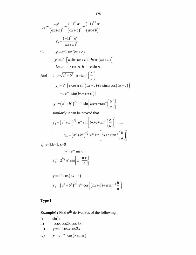
175

1 2 12 22

2 2 2 2

1 1a aa y

ax b ax b ax b

11

n n

n n

a y

ax b

9) sinax y e bx c

1 sin cosax y e a bx c b bx c

cos sin Let a = r , b = r ,

And 2 2 -1 r= a =tan

bb

a

1 y cos sin sin cosaxe r bx c r bx c

sinaxre bx c

1

2 2 ax -12

1 y a e sin x+c+tanb

b ba

it can be proved that similarly

2

2 2 ax -12

2 y a e sin x+c+tan ........b

b ba

n

2 2 ax -12

n y a e sin x+c+tanb

b ba

a=1,b=1, c=0If

ax y e sin x

nx2

n

n y 2 e sin x+

4

ax y e cos bx c

n

2 2 ax 12

n y e cos tanb

a b bx c na

Type I

Example1: Find nth derivatives of the following :

i) 3sin x

ii) osx cos2x cos 3xc

iii) xy e cos cos2x x

iv) cos cos sinxy e x

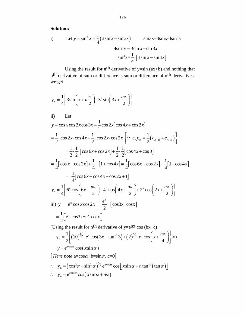
176

Solution:

i) Let 3 31sin 3sin sin3 sin3x=3sinx-4sin

4y x x x x

3 4sin 3sin sin3x x x

3 1 sin x= 3sin sin3

4x x

Using the result for nth derivative of y=sin (ax+b) and nothing that

nth derivative of sum or difference is sum or difference of nth derivatives,

we get

n

1y 3sin 3 sin 3

4 2 2

n nx n x

ii) Let

1

cos cos 2 cos3 cos 2 cos 4 cos 22

y x x x x x x

A B

1 1 1cos 2 cos 4 cos 2 cos 2 c c

2 2 2A B A Bx x x x c c

1 1 1 1cos6 cos 2 cos 4 cos0

2 2 2 2x x x

1 1 1 1

cos cos 2 1 cos 4 cos6 cos 2 1 cos 44 4 4 4

x x x x x x

1 cos6 cos 4 cos 2 14

x x x

n n n16 cos 6 4 cos 4 2 cos 2

4 2 2 2n

n n ny x x x

iii)

xy e cos cos 2 cos3x+cosx 2

xex x

x x1 e cos3x+e cosx

2

[Using the result for nth derivative of y=eax cos (bx+c)

12 2n

1 y 10 cos 3 tan 3 2 cos

2 4

n nx x n

e x e x

iv)

cos cos sinxy e x

a=cos , b=sin , c=0Here note

2 2 cos 12

n y cos sin cos sin tan tann

xe x n

cos

n y cos sinxe x n

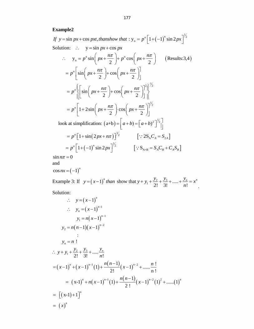
177

Example2

1

2

n sin cos , : y 1 1 sin 2nnIf y px pxt thanshow that p px

Solution: y sin cospx px

n y sin cos Results:3,42 2

n nn np px p px

sin cos2 2

n n np px px

12 2

sin cos2 2

n n np px px

12

1 2sin cos 2 2

n n np px px

1

2 2 look at simplification: a+b ) ) a b a b

1

2A 2 1 sin 2 2Sn

A Ap px n C S

1

2

A+B 1 1 sin 2 Snn

A B A Bp px S C C S

sin 0n

and

cos 1n

nx

Example 3: If 1n

y x than show that 32

1 .....2! 3! !

nny yyy y x

n

.

Solution:

1n

y x

1

1n

ny x

1

1 1n

y n x

2

2 1 1n

y n n x

:

!ny n

321 .....

2! 3! !

ny yyy y

n

1 21 !

1 1 1 1 ......2! n !

n n nn n nx x x

1 2 21

x-1 1 1 1 1 ...... 12 !

n n n nn nn x x

x-1 1n

n

x

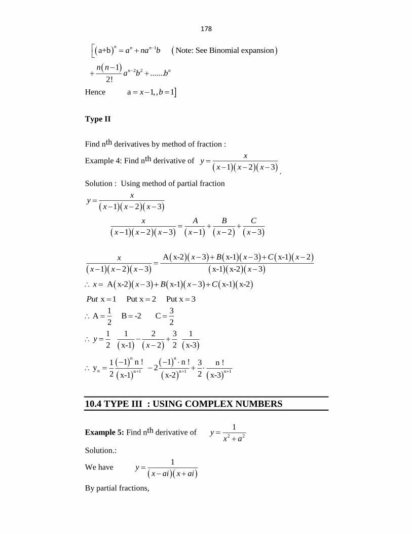
178

1 a+b Note: See Binomial expansionn n na na b

2 21

.......2!

n nn n

a b b

Hence a 1,, 1x b

Type II

Find nth derivatives by method of fraction :

Example 4: Find nth derivative of 1 2 3

xy

x x x

.

Solution : Using method of partial fraction

1 2 3

xy

x x x

1 2 3 1 2 3

x A B C

x x x x x x

A x-2 3 x-1 3 x-1 2

1 2 3 x-1 x-2 3

x B x C xx

x x x x

A x-2 3 x-1 3 x-1 x-2x x B x C

x 1 Put x 2 Put x 3Put

1 3A B -2 C

2 2

1 1 2 3 1

2 x-1 2 2 x-3

yx

n n

n n 1 n 1 n 1

1 n ! 1 n !1 3 n !y 2

2 2x-1 x-2 x-3

10.4 TYPE III : USING COMPLEX NUMBERS

Example 5: Find nth derivative of 2 2

1y

x a

Solution.:

We have

1y

x ai x ai

By partial fractions,

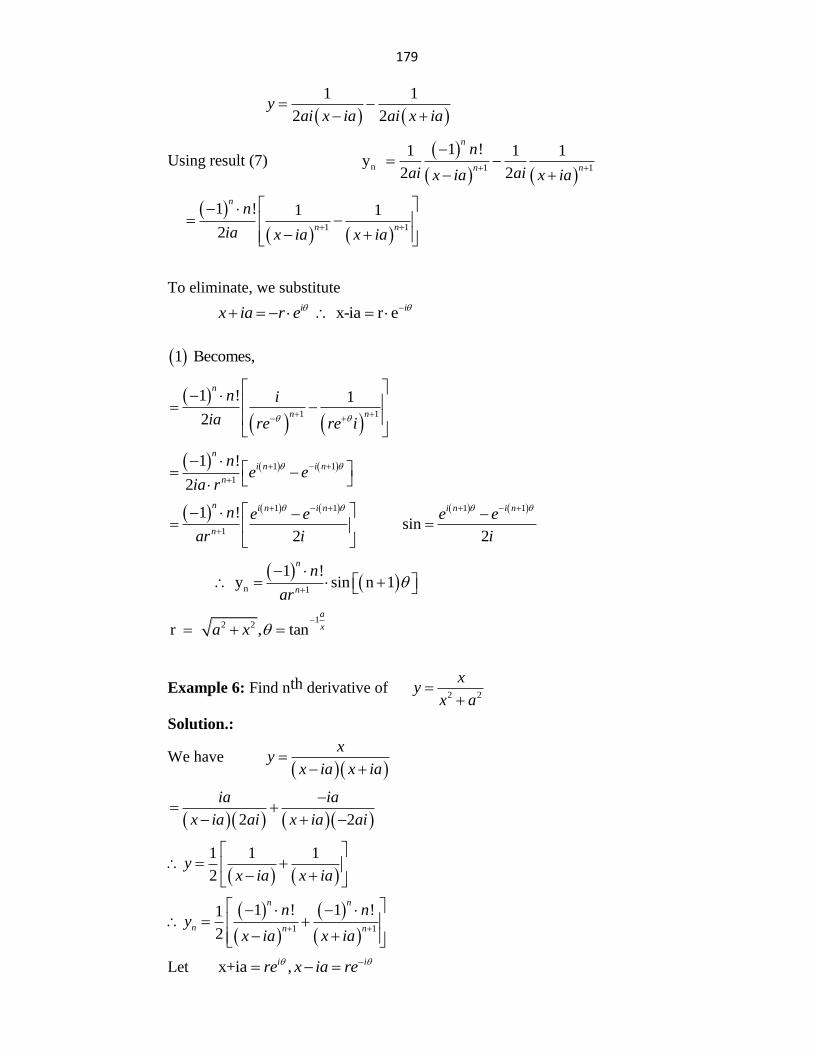
179

1 1

2 2y

ai x ia ai x ia

Using result (7)

n 1 1

1 !1 1 1y

2 2

n

n n

n

ai aix ia x ia

1 1

1 ! 1 1

2

n

n n

n

ia x ia x ia

To eliminate, we substitute

x-ia r ei ix ia r e

1 Becomes,

1 1

1 ! 1

2

n

n n

n i

ia re re i

1 1

1

1 !

2

n

i n i n

n

ne e

ia r

1 1 1 1

1

1 ! sin

2 2

n i n i n i n i n

n

n e e e e

ar i i

n 1

1 ! y sin n 1

n

n

n

ar

12 2r , tan

a

xa x

Example 6: Find nth derivative of 2 2

x

yx a

Solution.:

We have

xy

x ia x ia

2 2

ia ia

x ia ai x ia ai

1 1 1

2y

x ia x ia

1 1

1 ! 1 !1

2

n n

n n n

n ny

x ia x ia

Let x+ia ,i ire x ia re

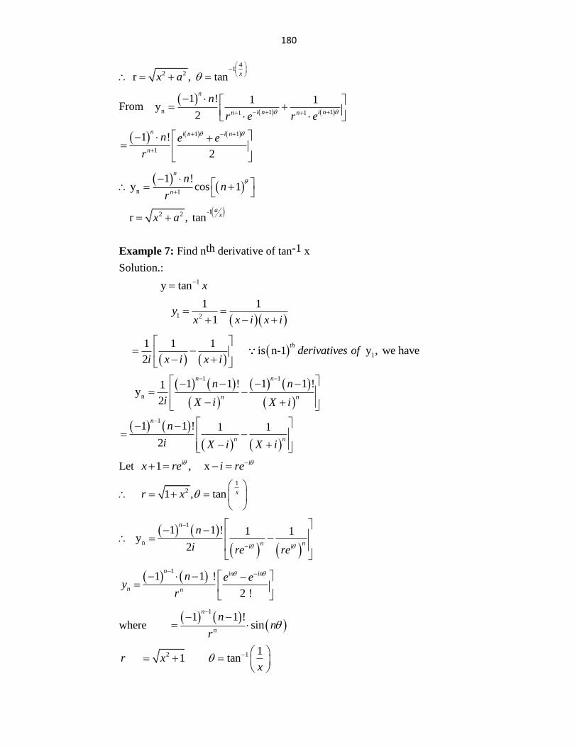
180

41

2 2 r , tan xx a

From

n 1 11 1

1 ! 1 1y

2

n

i n i nn n

n

r e r e

1 1

1

1 !

2

n i n i n

n

n e e

r

n 1

1 !y cos 1

n

n

nn

r

-12 2 r , tana

xx a

Example 7: Find nth derivative of tan-1 x

Solution.:

1 y tan x

1 2

1 1

1y

x x i x i

1

1 1 1 is n-1 y , we have

2

thderivatives of

i x i x i

1 1

n

1 1 ! 1 1 !1 y

2

n n

n n

n n

i X i X i

11 1 ! 1 1

2

n

n n

n

i X i X i

Let 1 , xi ix re i re

1

2 1 , tan xr x

1

n

1 1 ! 1 1 y

2

n

n ni i

n

i re re

1

1 1 !

2 !

n in in

n n

n e ey

r

where

1

1 1 ! sin

n

n

nn

r

2 1 1 1 tanr x

x

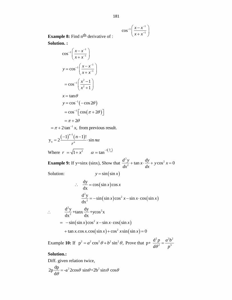
181

Example 8: Find nth derivative of :

11

1cos

x x

x x

Solution. :

1

1

1cos

x x

x x

1

1

1cos

x xy

x x

2

1

2

1 cos

1

x

x

tanx

1cos cos2y

1 cos cos 2

2 1 2 tan , from previous result.x

1

n

1 1 !y 2 sin

n

n

nn

r

Where 112 1 tan xr x

Example 9: If y=sinx (sinx), Show that 2

2

2tan cos 0

d y dyx y x

dx dx

Solution: sin siny x

dy

cos sin cosdx

x x

2

2

2

d y sin sin cos sin cos sin

dxx x x x

22

2

d y dy +tanx +ycos x

dx dx

2 sin sin cos sin cos sinx x x x

2 tan .cos .cos sin cos sin sin 0x x x x x

Example 10: If 2 2 2 2 2 p cos sin ,a b Prove that2 2 2

2 3

d p+

p a b

d p

Solution.:

Diff. given relation twice,

2 2dp2p -a 2cos sin +2b sin cos

d

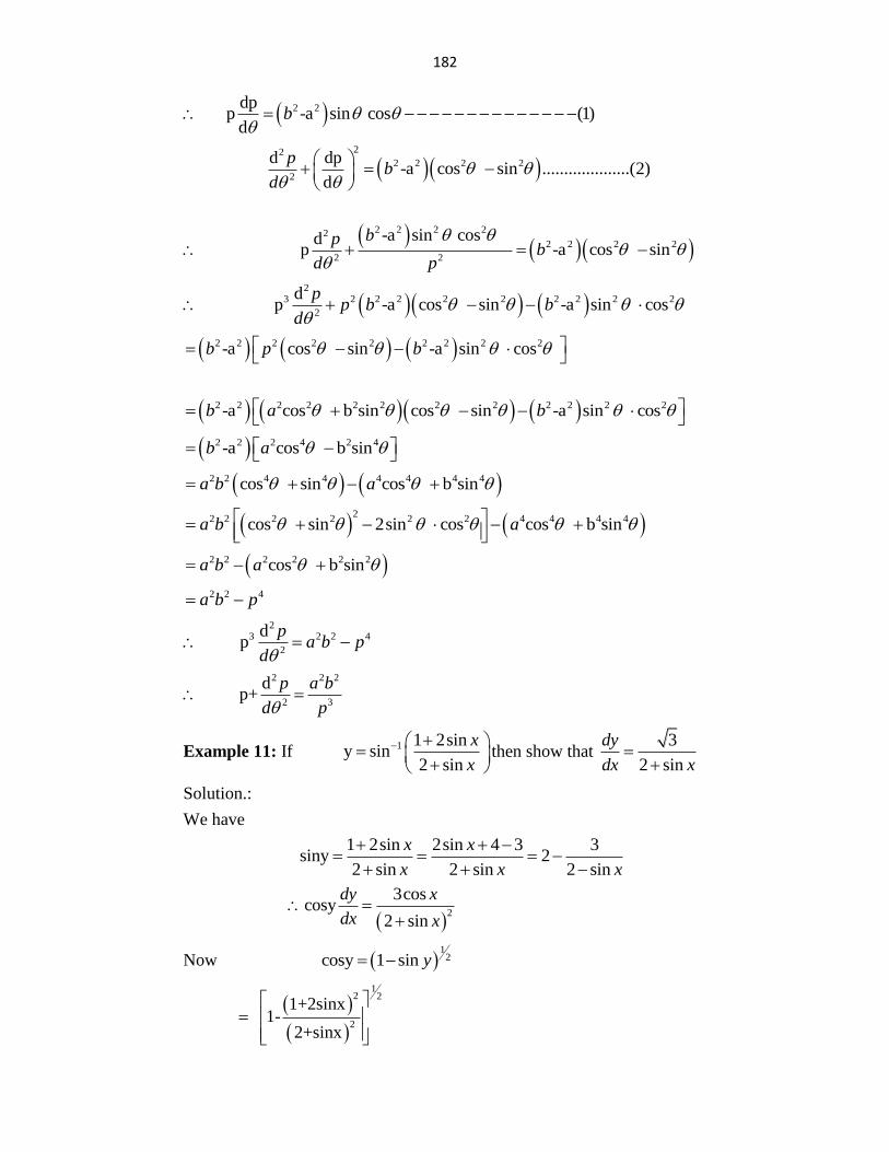
182

2 2dp p -a sin cos (1)

db

22

2 2 2 2

2

d dp -a cos sin ....................(2)

d

pb

d

2 2 2 222 2 2 2

2 2

-a sin cos d p -a cos sin

bpb

d p

2

3 2 2 2 2 2 2 2 2 2

2

d p -a cos sin -a sin cos

pp b b

d

2 2 2 2 2 2 2 2 2-a cos sin -a sin cos b p b

2 2 2 2 2 2 2 2 2 2 2 2-a cos b sin cos sin -a sin cosb a b

2 2 2 4 2 4-a cos b sinb a

2 2 4 4 4 4 4 4cos sin cos b sina b a

2

2 2 2 2 2 2 4 4 4 4cos sin 2sin cos cos b sina b a

2 2 2 2 2 2cos b sina b a

2 2 4a b p

23 2 2 4

2

d p

pa b p

d

2 2 2

2 3

d p+

p a b

d p

Example 11: If 1 1 2sin

y sin2 sin

x

x

then show that

3

2 sin

dy

dx x

Solution.:

We have

1 2sin 2sin 4 3 3

siny 22 sin 2 sin 2 sin

x x

x x x

2

3coscosy

2 sin

dy x

dx x

Now 1

2 cosy 1 sin y

12 2

2

1+2sinx 1-

2+sinx

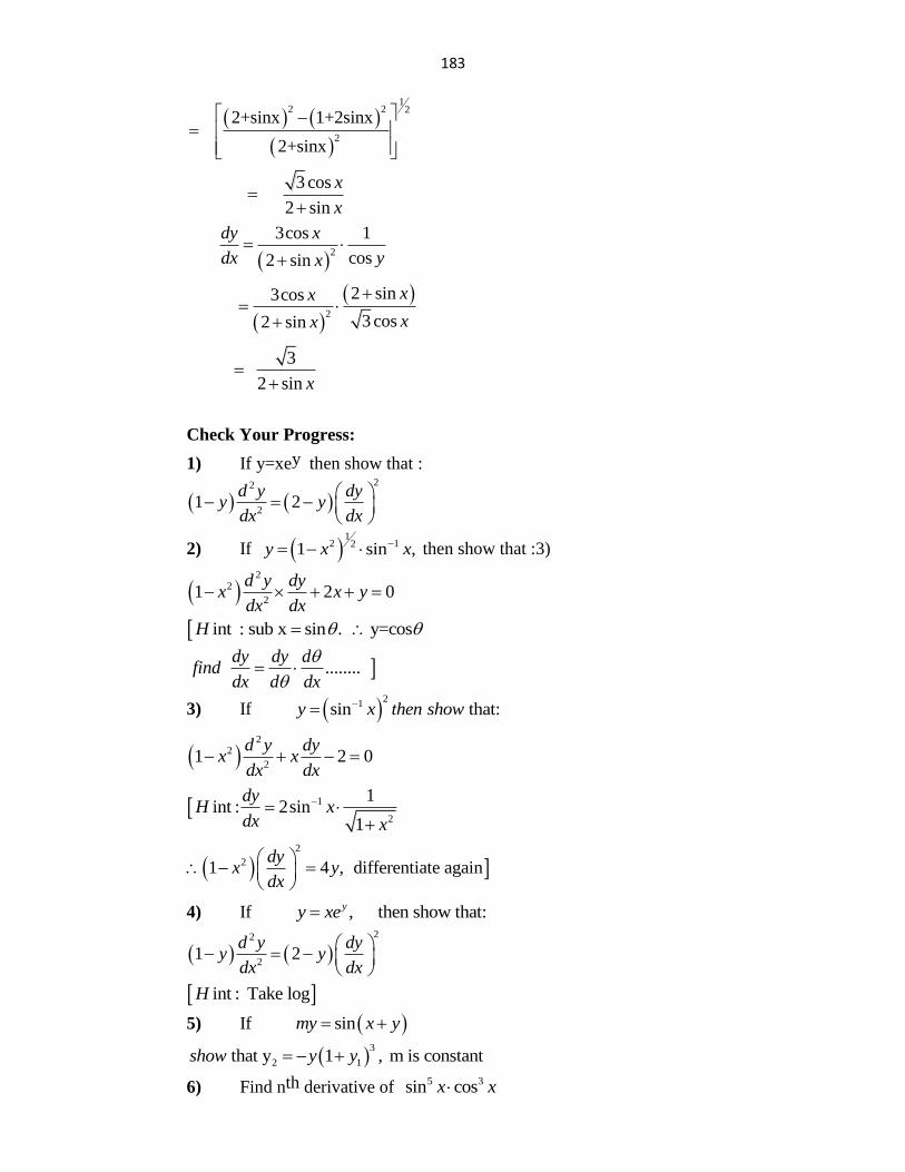
183

12 2 2

2

2+sinx 1+2sinx

2+sinx

3 cos

2 sin

x

x

2

3cos 1

cos2 sin

dy x

dx yx

2

2 sin3cos

3 cos2 sin

xx

xx

3

2 sin x


1) If y=xey then show that :

22

21 2

d y dyy y

dx dx

2) If 1

2 121 sin ,y x x then show that :3)

2

2

21 2 0

d y dyx x y

dx dx

int : sub x sin . y=cosH

........dy dy d

finddx d dx

3) If 2

1sin that:y x then show

2

2

21 2 0

d y dyx x

dx dx

1

2

1int : 2sin

1

dyH x

dx x

2

21 4 , differentiate againdy

x ydx

4) If , then show that:yy xe

22

21 2

d y dyy y

dx dx

int : Take logH

5) If sinmy x y

3

2 1 that y 1 , m is constantshow y y

6) Find nth derivative of 5 3sin cosx x

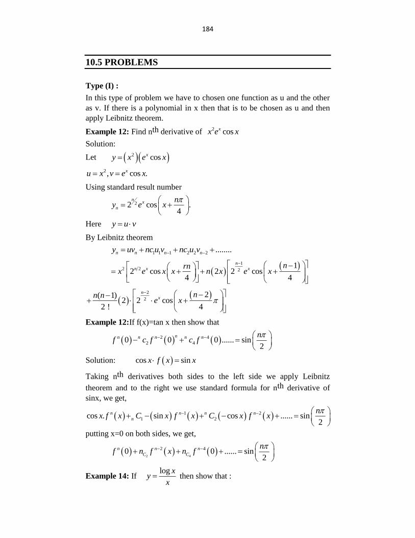
184

10.5 PROBLEMS

Type (I) :

In this type of problem we have to chosen one function as u and the other

as v. If there is a polynomial in x then that is to be chosen as u and then

apply Leibnitz theorem.

Example 12: Find nth derivative of 2 cosxx e x

Solution:

Let 2 cosxy x e x

2 , cos .xu x v e x

Using standard result number

22 cos .4

nx

n

ny e x

Here y u v

By Leibnitz theorem

1 1 1 2 2 2 ........n n n ny uv nc u v nc u v

1

2 2 21

2 cos 2 2 cos4 4

n

n x xnrn

x e x x n x e x

2

22( 1)

2 2 cos2 ! 4

n

xnn n

e x

Example 12:If f(x)=tan x then show that

2 4

2 40 0 0 ...... sin2

nn n n n n nf c f c f

Solution: cos sinx f x x

Taking nth derivatives both sides to the left side we apply Leibnitz

theorem and to the right we use standard formula for nth derivative of

sinx, we get,

1 2

1 2cos . sin cos ...... sin2

n n n n

n

nx f x C x f x C x f x

putting x=0 on both sides, we get,

2 4

2 40 0 ...... sin2

n n n

C C

nf n f x n f

Example 14: If log x

yx

then show that :

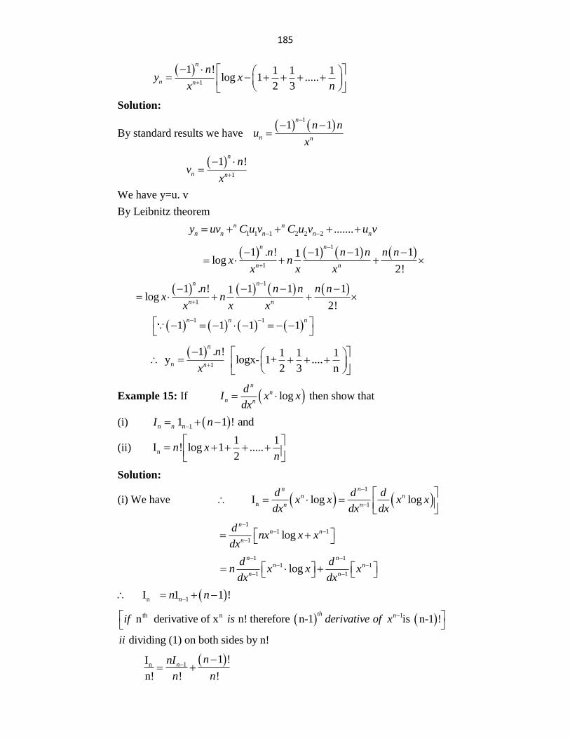
185

1

1 ! 1 1 1log 1 .....

2 3

n

n n

ny x

x n

Solution:

By standard results we have

11 1

n

n n

n nu

x

1

1 !n

n n

nv

x

We have y=u. v

By Leibnitz theorem

1 1 1 2 2 2 .......n n

n n n n ny uv C u v C u v u v

1

1

1 . ! 1 1 11 log

2!

n n

n n

n n n n nx n

x x x

1

1

1 . ! 1 1 11 log

2!

n n

n n

n n n n nx n

x x x

1 1

1 1 1 1n n n

n 1

1 . ! 1 1 1 y logx- 1+ ....

2 3 n

n

n

n

x

Example 15: If logn

n

n n

dI x x

dx then show that

(i) 11 1 ! andn n nI n

(ii) n

1 1I ! log 1 .....

2n x

n

Solution:

(i) We have 1

n 1 I log log

n nn n

n n

d d dx x x x

dx dx dx

1

1 1

1log

nn n

n

dnx x x

dx

1 1

1 1

1 1 log

n nn n

n n

d dn x x x

dx dx

n 1 I 1 1 !nn n

th n 1 n derivative of x n! therefore n-1 is n-1 !

dividing (1) on both sides by n!

th nif is derivative of x

ii

1n1 !I

n! ! !

nnnI

n n

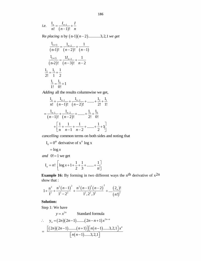
186

1nI

. . n! 1 !

nI Ii e

n n

Re n by n-1 2 ............3,2,1 placing n we get

n-1 2

1 1 1

n-1 ! 2 ! 1

n

n n

n-2 3

1 1 1

n-2 ! 3 ! 2

nI

n n

2 11 1 1

2! 1 2

0111

11! 0!

all the results columnwise we get,Adding

1 2n 2 1

1 11 1 1 .......

n! 1 ! 2 ! 2! 1!

n n

n n

1 2 01

1 1 11 .......

1 ! 2 ! 2! 0!

n n

n n

1 1 1 1 ....... 1

n 1 2 2n n

common terms on both sides and noting that cancelling

0

0 I 0 derivative of x log xth

log x

0! 1 we getand

n

1 1 1 I ! log 1 .......

2 3 nn x

Example 16: By forming in two different ways the nth derivative of x2n

show that :

22 22 22

22 2 2 2 2 2

n 1 n 1 2 2 !n 1 ....

1 1 2 1 ,2 ,3 !

nn n n

n

Solution:

Step 1: We have

2 Standard formulany x

2

n y 2 2 1 ........ 2 1 n nn n n n x

2 2 1 ........ 1 1 ......3,2,1

1 ......3,2,1

nn n n n n x

n n

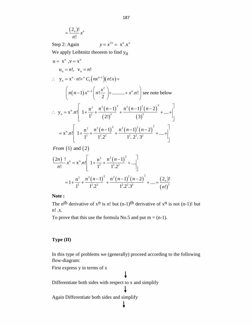
187

2 !

!

n nxn

Step 2: Again 2 n n x .x ny x

We apply Leibtnitz theorem to find yn nu x ,v xn

n n u !, v !n n

n 1

n 1 y x ! !n nn C nx n x

2

2 1 ! .......... . ! see note below2

n nxn n x n x n

22 22 22n

n 2 22

n 1 n 1 2n y x . ! 1 ....

1 2! 3

n n nn

22 22 22

n

2 2 2 2 2 2

n 1 n 1 2n x . ! 1 ....

1 1 .2 1 . 2 . 3

n n nn

1 and 2From

222

n

2 2 2

2 ! n 1nx . ! 1 ....

! 1 1 .2

nn n

x nn

22 22 22

22 2 2 2 2 2

n 1 n 1 2 2 !n 1 ....

1 1 .2 1 .2 .3 !

nn n n

n

Note :

The nth derivative of xn is n! but (n-1)th derivative of xn is not (n-1)! but

n! .x.

To prove that this use the formula No.5 and put m = (n-1).

Type (II)

In this type of problems we (generally) proceed according to the following

flow-diagram:

First express y in terms of x

Differentiate both sides with respect to x and simplify

Again Differentiate both sides and simplify

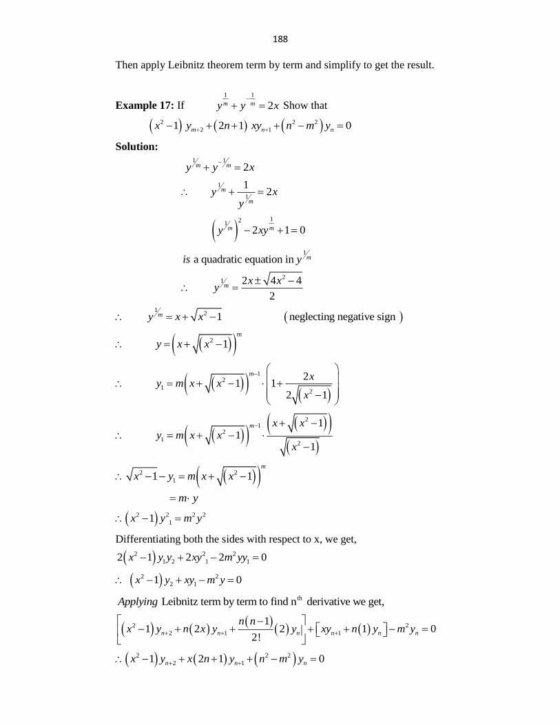
188

Then apply Leibnitz theorem term by term and simplify to get the result.

Example 17: If 1 1

2m my y x

Show that

2 2 2

2 11 2 1 0m n nx y n xy n m y

Solution:

1 1

2m my y x

1

1

1 2m

m

y xy

12

1

2 1 0m my xy

1

a quadratic equation in mis y

2

1 2 4 4

2m

x xy

1

2 1 neglecting negative sign my x x

m

2 1 y x x

12

12

2 1 1

2 1

m xy m x x

x

21

2

12

1 1

1

m x xy m x x

x

2 2

11 1m

x y m x x

m y

2 2 2 2

11x y m y

Differentiating both the sides with respect to x, we get,

2 2 2

1 2 1 12 1 2 2 0x y y xy m yy

2 2

2 1 1 0x y xy m y

th Leibnitz term by term to find n derivative we get,Applying

2 2

2 1 1

11 2 2 1 0

2!n n n n n n

n nx y n x y y xy n y m y

2 2 2

2 11 2 1 0n n nx y x n y n m y

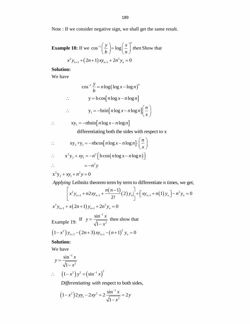
189

Note : If we consider negative sign, we shall get the same result.

Example 18: If we 1cos log

ny x

thenb n

Show that

2 2

2 12 1 2 0n n nx y n xy n y

Solution:

We have

1cos log log logny

n x nb

y bcos log logn x n n

1 y b in log logn

s n x n nx

1 xy b in log logn s n x n n

differentiating both the sides with respect to x

2 1 xy +y b os log logn

n c n x n nx

2 2

2 1 x y bcos log logxy n n x n n

2 n y

2 2

2 1x y 0xy n y

Leibnitz theorem term by term to differentiate n times, we get, Applying

2 2

2 1 1

12 2 1 0

2!n n n n n n

n nx y n xy y xy n y n y

2 2

2 12 1 2 0n n nx y x n y n y

Example 19: If

1

2

sin

1

xy

x

then show that

22

2 11 2 3 1 0n n nx y n xy n y

Solution:

We have

1

2

sin

1

xy

x

2

2 2 1 1 sinx y x

respect to both sides, Differentiating with

1

2 2

12

sin 1 2 2 2 2

1

xx yy xy y

x

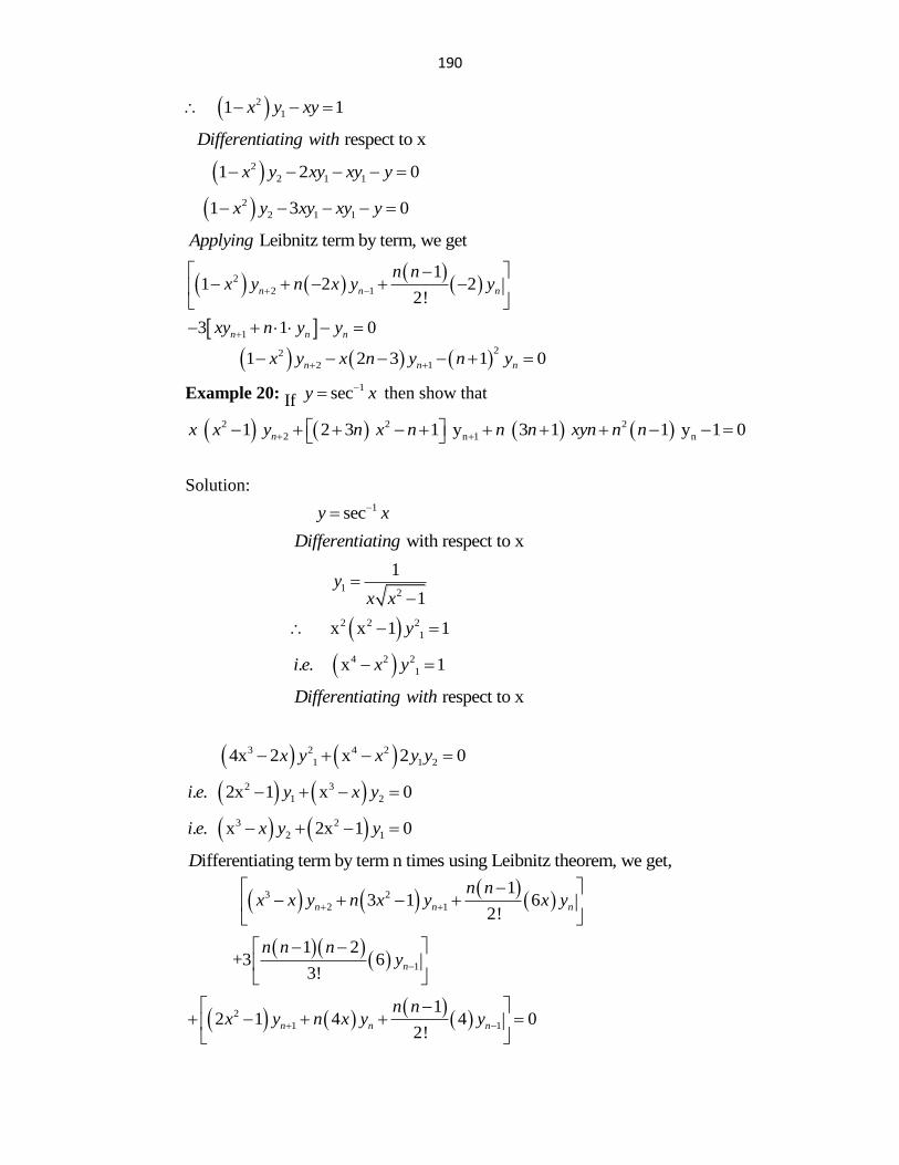
190

2

1 1 1x y xy

respect to xDifferentiating with

2

2 1 1 1 2 0x y xy xy y

2

2 1 1 1 3 0x y xy xy y

Leibnitz term by term, we getApplying

2

2 1

1

11 2 2

2!

3 1 0

n n n

n n n

n nx y n x y y

xy n y y

22

2 11 2 3 1 0n n nx y x n y n y

Example 20: If 1secy x then show that

2 2 2

2 n 1 n 1 2 3 1 y 3 1 1 y 1 0nx x y n x n n n xyn n n

Solution:

1secy x

with respect to xDifferentiating

12

1

1y

x x

2 2 2

1 x x 1 1y

4 2 2

1. . x 1i e x y

respect to xDifferentiating with

3 2 4 2

1 1 2 4x 2 x 2 0x y x y y

2 3

1 2. . 2x 1 x 0i e y x y

3 2

2 1. . x 2x 1 0i e x y y

ifferentiating term by term n times using Leibnitz theorem, we get,D

3 2

2 1

13 1 6

2!n n n

n nx x y n x y x y

1

1 2 +3 6

3!n

n n ny

2

1 1

12 1 4 4 0

2!n n n

n nx y n x y y

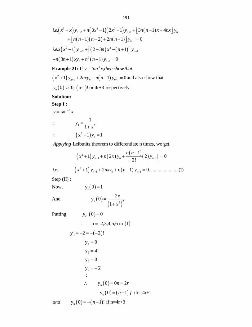
191

3 2 2

2 1. . 3 1 2 1 3 1 4n n ni e x x y n x x y n n x nx y

11 2 2 1 0nn n n n n y

2 2

2 1. . 1 2 3 1n ni e x x y n x n y

2

13 1 1 0n nn n xy n n y

Example 21: If -1y = tan x,then show that.

2

1 11 2 1 0n n nx y nxy n n y and also show that

0 0, n-1 ! or 4r+3ny is respectively

Solution:

Step I : 1tany x

1 2

1 y

1 x

2

1 x 1 y 1

Leibtnitz theorem to differentiate n times, we get, Applying

2

1 1

1 1 2 2 0

2!n n n

n nx y n x y y

2

1 1. . 1 2 1 0........................(1)n n ni e x y nxy n n y

Step (II) :

Now, 1 y 0 1

And

2 22

2 y 0

1

x

x

Putting 2 0 0y

n 2,3,4,5,6 in 1

3 y 2 2 !

4 y 0

5 y 4!

6 y 0

7 y 6!

n

:

y 0 0 2n r

n y 0 1 ifn=4r+1n f

n y 0 1 ! if n=4r+3and n

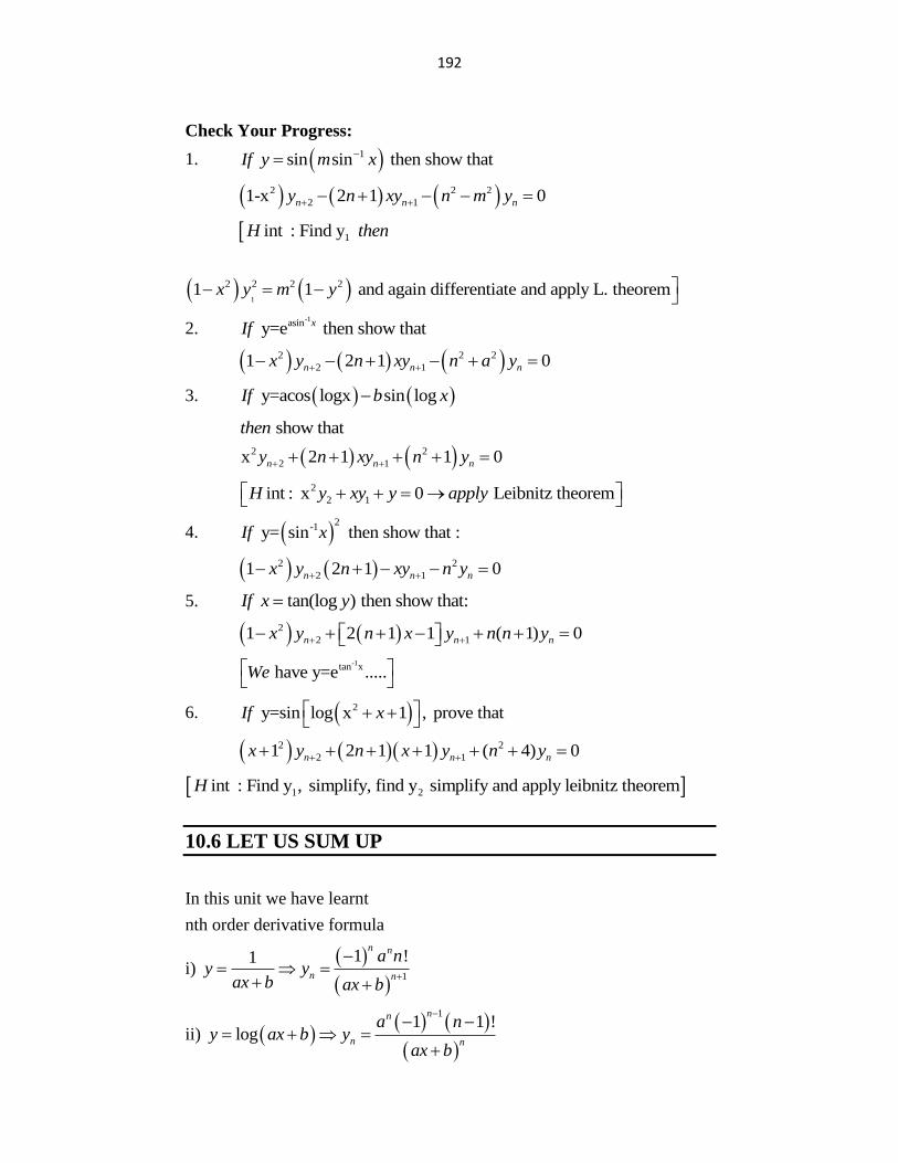
192


1. 1 sin sin then show thatIf y m x

2 2 2

2 11-x 2 1 0n n ny n xy n m y

1int : Find y H then

1

2 2 2 21 1 and again differentiate and apply L. theoremx y m y

2. -1asin y=e then show that xIf

2 2 2

2 11 2 1 0n n nx y n xy n a y

3. y=acos logx sin logIf b x

show thatthen

2 2

2 1x 2 1 1 0n n ny n xy n y

2

2 1int : x 0 Leibnitz theoremH y xy y apply

4. 2

-1 y= sin then show that :If x

2 2

2 11 2 1 0n n nx y n xy n y

5. tan(log ) then show that:If x y

2

2 11 2 1 1 ( 1) 0n n nx y n x y n n y

-1tan x have y=e .....We

6. 2 y=sin log x 1 , prove thatIf x

2 2

2 11 2 1 1 ( 4) 0n n nx y n x y n y

1 2int : Find y , simplify, find y simplify and apply leibnitz theoremH

10.6 LET US SUM UP

In this unit we have learnt

nth order derivative formula

i)

1

1 !1n n

n n

a ny y

ax b ax b

ii)

11 1 !

log

nn

n n

a ny ax b y

ax b

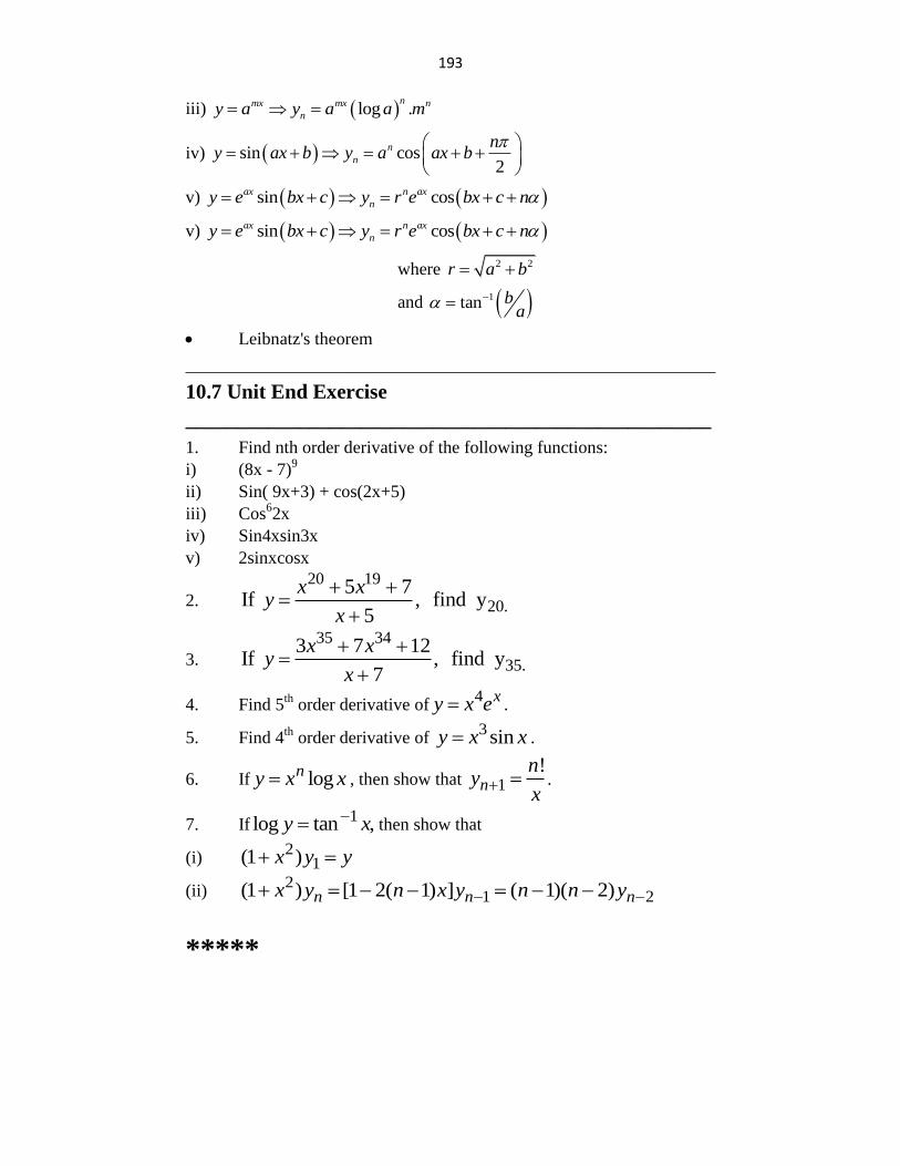
193

iii) log .nmx mx n

ny a y a a m

iv) sin cos2

n

n

ny ax b y a ax b

v) sin cosax n ax

ny e bx c y r e bx c n

v) sin cosax n ax

ny e bx c y r e bx c n

where 2 2r a b

and 1tan ba

Leibnatz's theorem

____________________________________________________________


___________________________________________________

1. Find nth order derivative of the following functions:

i) (8x - 7)9

ii) Sin( 9x+3) + cos(2x+5)

iii) Cos62x

iv) Sin4xsin3x

v) 2sinxcosx

2.

20 19

20.5 7

If , find y5

x xy

x

3.

35 34

35.3 7 12

If , find y7

x xy

x

4. Find 5th

order derivative of4 xy x e .

5. Find 4th

order derivative of 3 siny x x .

6. If logny x x , then show that 1!

nn

yx

.

7. If1log tan ,y x then show that

(i) 2

1(1 )x y y

(ii) 2

1 2(1 ) [1 2( 1) ] ( 1)( 2)n n nx y n x y n n y

*****

194

11

PARTIAL DIFFERENTIATION

UNIT STRUCTURE

11.1 Objective

11.2 Introduction

11.3 Partial Differential Coefficients

11.4 Total differentiation

11.5 Some additional results

11.6 TYPE - III Variable to be treated as constant

11.7 Let Us Sum Up


11.1 OBJECTIVE


Find Partial Differentiation.

Total Partial derivative

Euler's theorem

Approximation and error

Maxima and Minima

11.2 INTRODUCTION

So far, we have been concerned with a functions of a variable, but in many

problems in science and mathematics we have to deal with functions of

two or more independent variables.

e.g. the lift L of an aeroplane wing is a function of three independent

variables : A, the area of the wing, V, the speed at which the wing is

moving; and P the density of the air. The law is 2L Akv p

In the language of mathematics, if variable u has one definite value for any

given values of x,y,z then u is defined as a function of x,y,z.We represent

it as

u= f(x,y,z)

Note that u is independent variable and x,y,z are indepedent variables.

This relation is written as - , ,u x y z

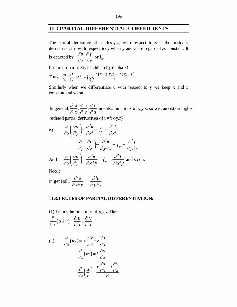
195

11.3 PARTIAL DIFFERENTIAL COEFFICIENTS

The partial derivative of u= f(x,y,z) with respect to x is the oridnary

derivative of u with respect to x when y and z are regarded as constant. It

is denoted by x, or f .u f

x x

(To be pronounced as dabba u by dabba x)

Thus,

x

, , , ,, or f

x®o

f x h y z f x y zu f

x x hlim

Similarly when we differentiate u with respect to y we keep x and z

constant and so on

.

u u uIn general, , , are also functions of x,y,z, so we can obtain higher

x y z

ordered partial derivatives of u=f(x,y,z)

e.g 2 2

2 2xx

u u ff

x y x x

2 2

yx

u u ff

y x y x y x

And 2 2

and so on. xy

u u ff

x y x y x y

Note :

In general , 2 2

u u

x y y x

11.3.1 RULES OF PARTIAL DIFFERENTIATION:

(1) Let,u v be functions of x,y,z Then

u v

x x xu v

(2) u +vv u

uvx x x

v

kv kx x

2

u vv u

u x x

x v v

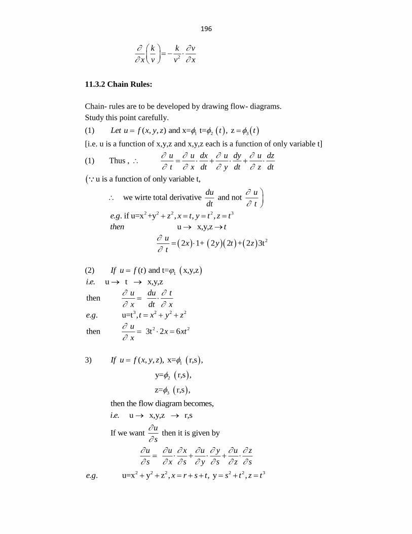
196

2

k k v

x v v x

11.3.2 Chain Rules:

Chain- rules are to be developed by drawing flow- diagrams.

Study this point carefully.

(1) 1 2 3 ( , , ) and x= t= , zLet u f x y z t t

[i.e. u is a function of x,y,z and x,y,z each is a function of only variable t]

(1) Thus ,

u u dx u dy u dz

t x dt y dt z dt

u is a function of only variable t,

we wirte total derivative and not

du u

dt t

2 2 2 2 3. . if u=x +y , , ,e g z x t y t z t

u x,y,zthen t

2 2 1+ 2 2 + 2 3t

ux y t z

t

(2) 1 ( ) and t= x,y,zIf u f t

. . u t x,y,zi e

then

u du t

x dt x

3 2 2 2. . u=t ,e g t x y z

2 2 then 3t 2 6

ux xt

x

3) 1 ( , , ), x= r,s ,If u f x y z

2 y= r,s ,

3 z= r,s ,

then the flow diagram becomes,

. . u x,y,z r,si e

If we want then it is given byu

s

u u x u y u z

s x s y s z s

2 2 2 2 2 3. . u=x y z , , y ,e g x r s t s t z t

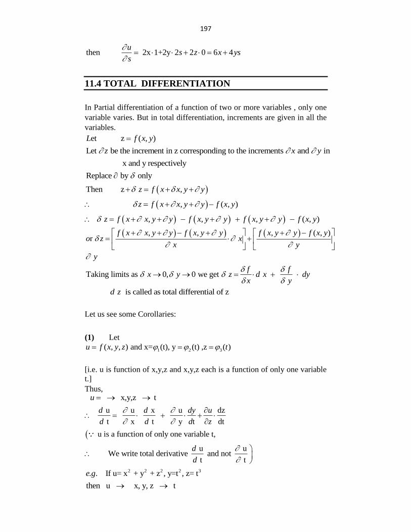
197

then 2x 1+2y 2 2 0 6 4u

s z x yss

11.4 TOTAL DIFFERENTIATION

In Partial differentiation of a function of two or more variables , only one

variable varies. But in total differentiation, increments are given in all the

variables.

et z ( , )L f x y

Let be the increment in z corresponding to the increments and inz x y

x and y respectively

Replace by only

Then z , z f x x y y

, ( , )z f x x y y f x y

, , , ( , )z f x x y y f x y y f x y y f x y

, , , ( , )r

f x x y y f x y y f x y y f x yo z x

x y

y

Taking limits as 0, 0 we get

f fx y z d x dy

x y

is called as total differential of zd z

Let us see some Corollaries:

(1) Let

1 2 3( , , ) and x= (t), y (t) ,z ( )u f x y z t

[i.e. u is function of x,y,z and x,y,z each is a function of only one variable

t.]

Thus, x,y,z tu

u u x u dz

t x t y t dt

u is a function of only one variable t,

d d dy u

d d d z

u u We write total derivative and not

t t

d

d

2 2 2 2 3. . If u= x + y + z , y=t , z= t e g

then u x, y, z t

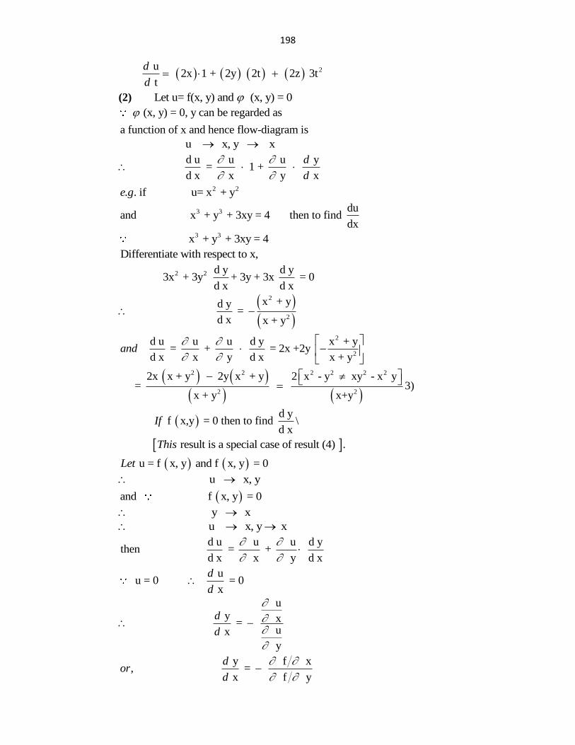
198

2 u 2x 1 + 2y 2t 2z 3t

t

d

d

(2) Let u= f(x, y) and (x, y) = 0

(x, y) = 0, y can be regarded as

a function of x and hence flow-diagram is

u x, y x

d u u u y = 1 +

d x x y x

d

d

2 2. . if u= x + y e g

3 3 duand x + y + 3xy = 4 then to find

dx

3 3 x + y + 3xy = 4

Differentiate with respect to x,

2 2 d y d y 3x + 3y + 3y + 3x = 0

d x d x

2

2

x + yd y =

d x x + y

2

2

d u u u d y x + y = + = 2x +2y

d x x y d x x + yand

2 2 2 2 2 2

2 2

2x x + y 2y x + y 2 x - y xy - x y =

x + y x+y

3)

d y

f x,y = 0 then to find d x

If \

result is a special case of result (4) .This

u = f x, y and f x, y = 0Let

u x, y

and f x, y = 0

y x

u x, y x

d u u u d ythen = +

d x x y d x

u u = 0 = 0

x

d

d

u

y x = u x

y

d

d

y f x, =

x f y

dor

d

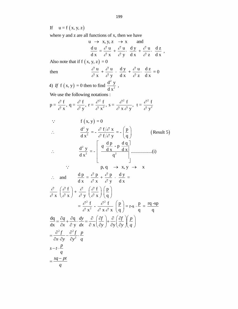
199

If u = f x, y, z

where y and z are all functions of x, then we have

u x, y, z x and

d u u u d y u d z = + + ,

d x x y d x z d x

Also note that if f x, y, z = 0

u u d y u d zthen + + = 0

x y d x z d x

4) 2

2

d y f x, y = 0 then to find ,

d xIf

We use the following notations : 2 2 2

2 2

f f f f fp = , q = , r = , s = , t =

x y x x y y

f x, y = 0

2

2

d y f x p = - = - Result 5

d x f y q

2

2 2

d p d q - p

d y d x d x = - ..................(i)d x q

q

p, q x, y x

d p p p d y and = + =

d x x y d x

f f p +

x x y x q

2 2

2

f f p p rq -sp = - = r-s =

x x x q q q

dq q

dx y x y

q dy f f p

x dx y y q

2 2

2

f f p

x y y q

ps t

q

sq pt

q

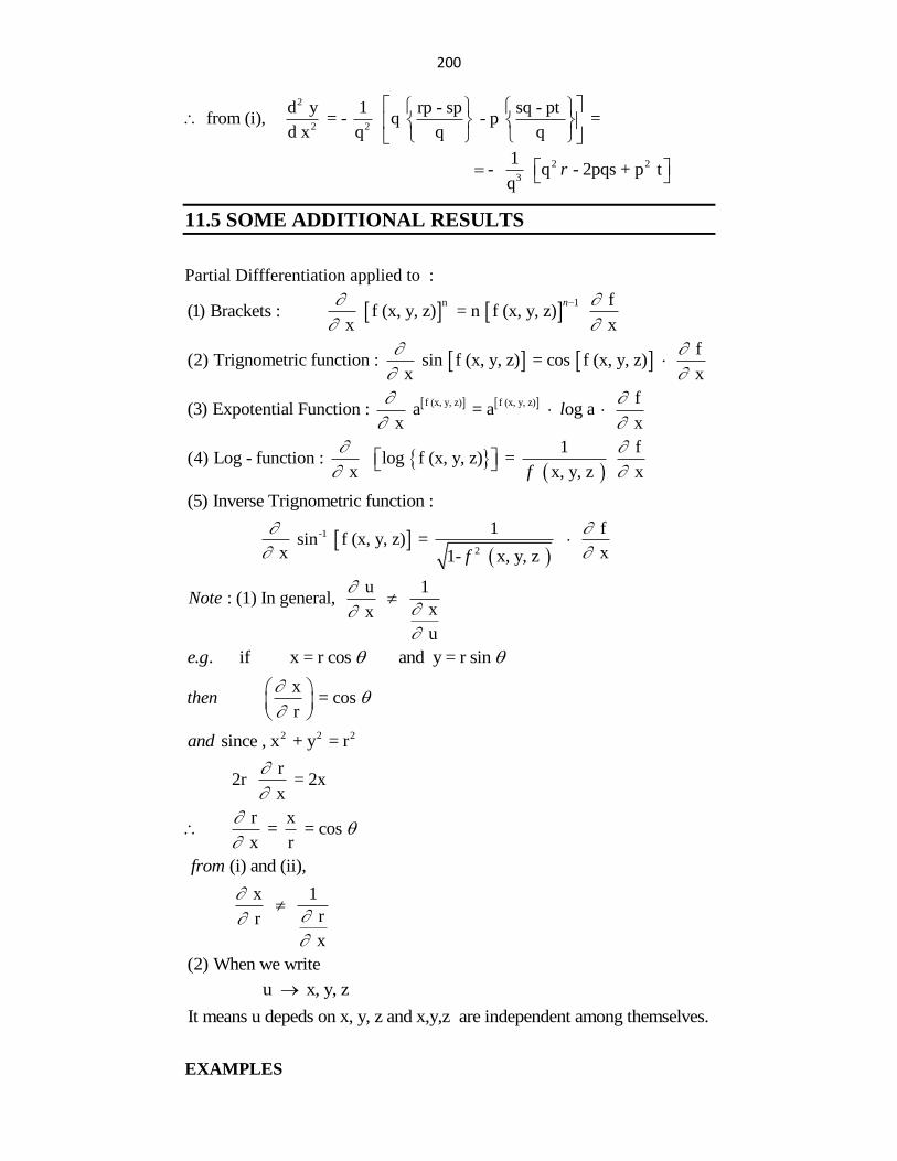
200

2

2 2

d y 1 rp - sp sq - pt from (i), = - q - p =

d x q q q

2 2

3

1 - q - 2pqs + p t

qr

11.5 SOME ADDITIONAL RESULTS

Partial Diffferentiation applied to :

n 1 f

(1) Brackets : f (x, y, z) = n f (x, y, z) x x

n

f

(2) Trignometric function : sin f (x, y, z) = cos f (x, y, z) x x

f (x, y, z) f (x, y, z) f(3) Expotential Function : a = a og a

x xl

1 f(4) Log - function : log f (x, y, z) =

x x, y, z xf

(5) Inverse Trignometric function :

-1

2

1 f sin f (x, y, z) =

x x1- x, y, z f

u 1 : (1) In general,

x x

u

Note

. . if x = r cos and y = r sin e g

x = cos

rthen

2 2 2 since , x + y = rand

r 2r = 2x

x

r x = = cos

x r

(i) and (ii),from

x 1

r r

x

(2) When we write

u x, y, z

It means u depeds on x, y, z and x,y,z are independent among themselves.

EXAMPLES

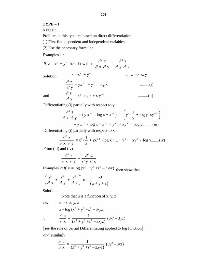
201

TYPE – I

NOTE :

Problem in this type are based on direct differentiation

(1) First find dependent and independent variables.

(2) Use the necessary formulae.

Examples 1 :

y x z = x + y then show that If2 2 z z

= x y y x

.

Solution:y x z = x + y z x, y

y-1 x z = yx + y log x .........(i)

y

y x-1 zand = x log x + x y ..........(ii)

y

Differentiating (i) partially with respect to y,

2

y-1 y-1 x x-1 z 1 = y x log x + x y + log y xy

x y y

y-1 y-1 x-1 x-1 = y x log x + x + y + xy log y..........(iii)

Differentiating (i) partially with respect to x,

2y y-1 x-1 x-1 z 1

= x + yx log x + 1 y + xy log y........(iv) x y x

From (iii) and (iv)

2 2 z z =

x y y x

Examples 2: 3 3 3 u = log (x + y +z 3 ) If xyz then show that

2

2

-9 + + u =

x y z x + y + z

Solution:

Note that u is a function of x, y, z

i.e. u x, y, z

3 3 3 u = log (x + y +z 3 )xyz

2

3 3 3

u 1 = (3x 3 )

x (x + y +z 3 )yz

xyz

the rule of partial Differentiating applied to log functionsee

similarlyand

2

3 3 3

u 1 = (3y 3 )

x (x + y +z 3 )xz

xyz

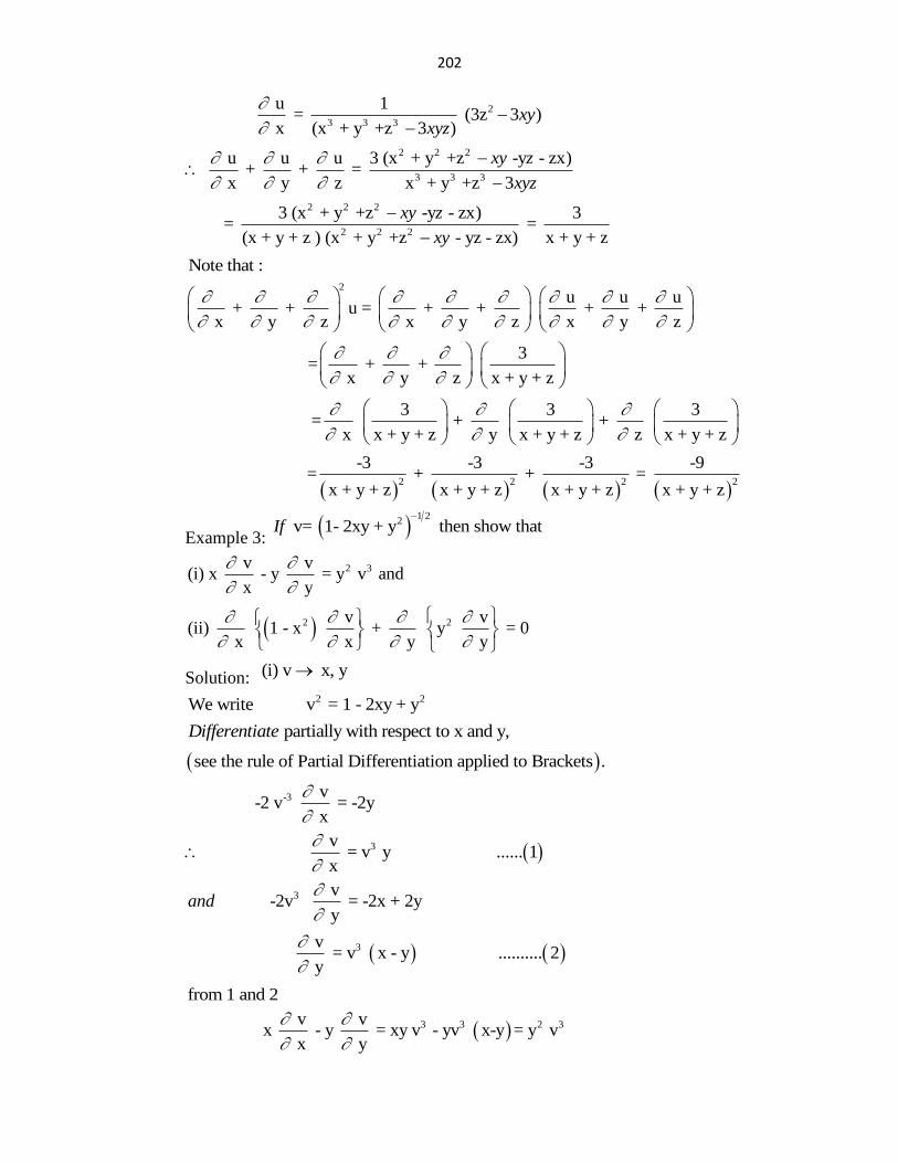
202

2

3 3 3

u 1 = (3z 3 )

x (x + y +z 3 )xy

xyz

2 2 2

3 3 3

u u u 3 (x + y +z -y - zx) + + =

x y z x + y +z 3

xy z

xyz

2 2 2

2 2 2

3 (x + y +z -y - zx) 3 = =

(x + y + z ) (x + y +z - yz - zx) x + y + z

xy z

xy

Note that : 2

u u u + + u = + + + +

x y z x y z x y z

3 = + +

x y z x + y + z

3 3 3 = + +

x x + y + z y x + y + z z x + y + z

2 2 2 2

-3 -3 -3 -9 = + + =

x + y + z x + y + z x + y + z x + y + z

Example 3:

1 22 v= 1- 2xy + y then show thatIf

2 3

2 2

v v(i) x - y = y v and

x y

v v(ii) 1 - x + y = 0

x x y y

Solution: (i) v x, y

2 2We write v = 1 - 2xy + y

partially with respect to x and y, Differentiate

see the rule of Partial Differentiation applied to Brackets .

-3 v -2 v = -2y

x

3 v = v y ...... 1

x

3 v -2v = -2x + 2y

yand

3 v = v x - y .......... 2

y

from 1 and 2

3 3 2 3 v v x - y = xy v - yv x-y = y v

x y

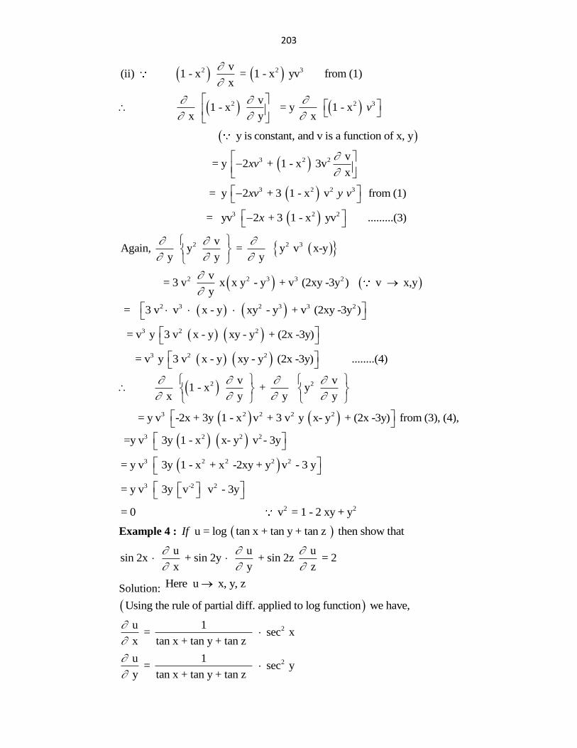
203

2 2 3 v(ii) 1 - x = 1 - x yv from (1)

x

2 2 3 v 1 - x = y 1 - x

x y xv

y is constant, and v is a function of x, y

3 2 2 v = y 2 + 1 - x 3v

xxv

3 2 2 3 = y 2 + 3 1 - x v from (1)xv y v

3 2 2 = yv 2 + 3 1 - x yv .........(3)x

2 2 3 v Again, y = y v x-y

y y y

2 2 3 3 2 v = 3 v x x y - y + v (2xy -3y ) v x,y

y

2 3 2 3 3 2 = 3 v v x - y xy - y + v (2xy -3y )

3 2 2 = v y 3 v x - y xy - y + (2x -3y)

3 2 2 = v y 3 v x - y xy - y (2x -3y) ........(4)

2 2 v v 1 - x + y

x y y y

3 2 2 2 2 = y v -2x + 3y 1 - x v + 3 v y x- y + (2x -3y) from (3), (4),

3 2 2 2 =y v 3y 1 - x x- y v - 3y

3 2 2 2 2= y v 3y 1 - x + x -2xy + y v - 3 y

3 -2 2= y v 3y v v - 3y

2 2= 0 v = 1 - 2 xy + y

Example 4 : u = log tan x + tan y + tan z then show that If

u u usin 2x + sin 2y + sin 2z = 2

x y z

Solution: Here u x, y, z

Using the rule of partial diff. applied to log function we have,

2 u 1 = sec x

x tan x + tan y + tan z

2 u 1 = sec y

y tan x + tan y + tan z

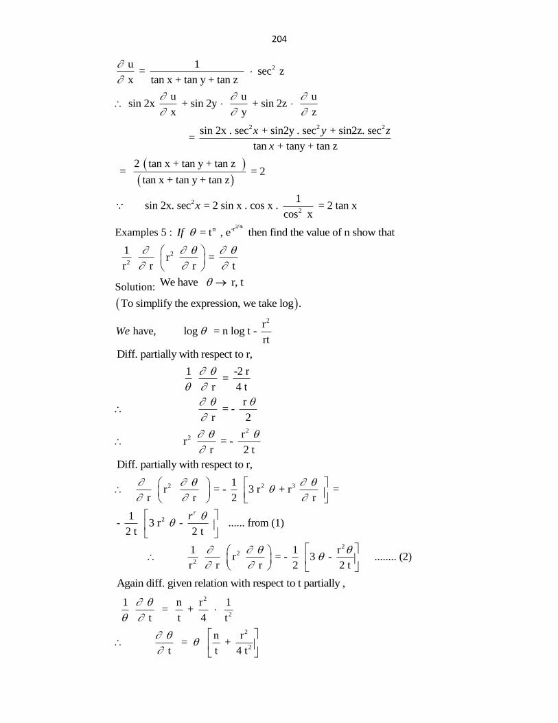
204

2 u 1 = sec z

x tan x + tan y + tan z

u u u sin 2x + sin 2y + sin 2z

x y z

2 2 2sin 2x . sec + sin2y . sec + sin2z. sec =

tan + tany + tan z

x y z

x

2 tan x + tan y + tan z = = 2

tan x + tan y + tan z

2

2

1 sin 2x. sec = 2 sin x . cos x . = 2 tan x

cos xx

Examples 5 : 2 4tn -r = t , e then find the value of n show thatIf

2

2

1 r = r r r t

Solution: We have r, t

To simplify the expression, we take log .

2r have, log = n log t -

rtWe

Diff. partially with respect to r,

1 -2 r =

r 4 t

r = -

r 2

22 r

r = - r 2 t

Diff. partially with respect to r,

2 2 3

2

1 r = - 3 r + r =

r r 2 r

1 - 3 r - ...... from (1)

2 t 2 t

rr

2

2

2

1 1 r r = - 3 - ........ (2)

r r r 2 2 t

Again diff. given relation with respect to t partially ,

2

2

1 n r 1 = +

t t 4 t

2

2

n r = +

t t 4 t

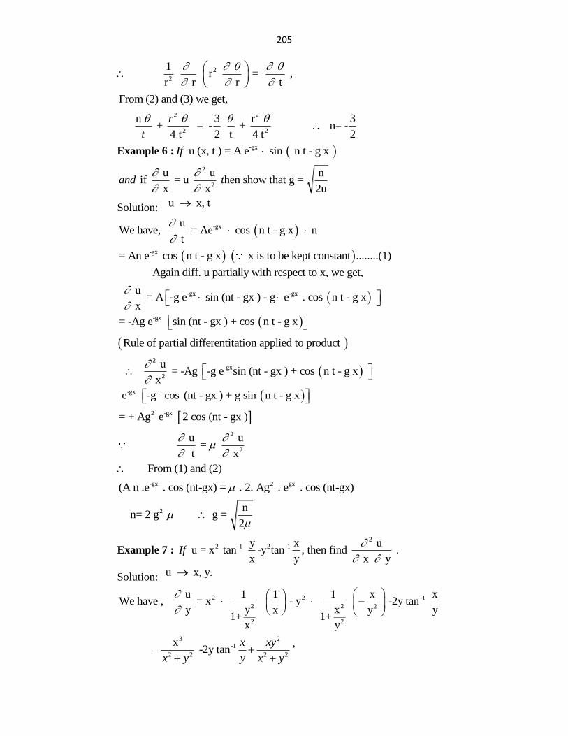
205

2

2

1 r = ,

r r r t

From (2) and (3) we get,

2 2

2 2

n 3 r 3 + = - + n= -

4 t 2 t 4 t 2

r

t

Example 6 : -gx u (x, t ) = A e sin n t - g x If

2

2

u u n if = u hen show that g =

x x 2uand t

Solution: u x, t

-gx uWe have, = Ae cos n t - g x n

t

-gx= An e cos n t - g x x is to be kept constant ........(1)

Again diff. u partially with respect to x, we get,

-gx -gx u = A -g e sin (nt - gx ) - g e . cos n t - g x

x

-gx= -Ag e sin (nt - gx ) + cos n t - g x

Rule of partial differentitation applied to product

2

-gx

2

u = -Ag -g e sin (nt - gx ) + cos n t - g x

x

-gx e -g cos (nt - gx ) + g sin n t - g x

2 -gx= + Ag e 2 cos (nt - gx )

2

2

u u =

t x

From (1) and (2)

-gx 2 gx(A n .e . cos (nt-gx) = . 2. Ag . e . cos (nt-gx)

2 n n= 2 g g =

2

Example 7 : 2

2 -1 2 -1y x u u = x tan -y tan , then find .

x y x yIf

Solution: u x, y.

2 2 -1

2 2 2

2 2

u 1 1 1 x xWe have , = x - y -2y tan

y x y x y y1+ 1+

x y

3 2

-1

2 2 2 2

x -2y tan

x xy

x y y x y

‟

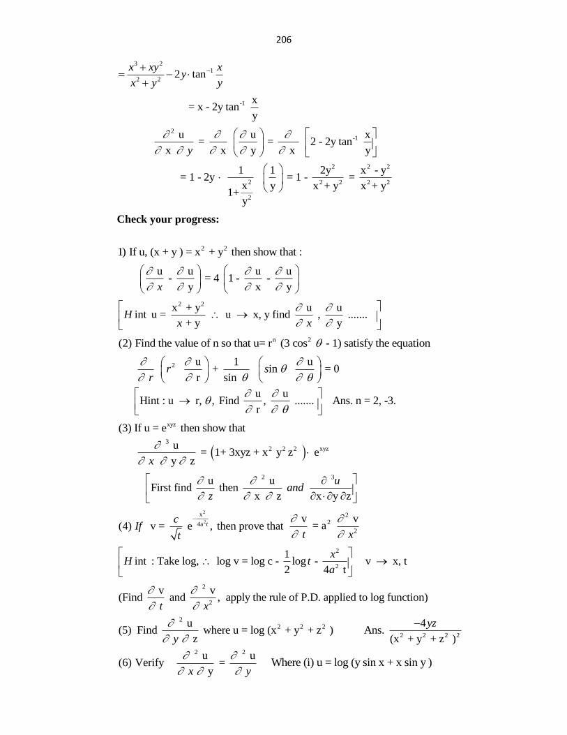
206

3 21

2 22 tan

x xy xy

x y y

-1 x = x - 2y tan

y

2-1 u u x

= = 2 - 2y tan x x y x yy

2 2 2

2 2 2 2 2

2

1 1 2y x - y = 1 - 2y = 1 - =

x y x + y x + y1+

y


2 21) If u, (x + y ) = x + y then show that :

u u u u - = 4 1 - -

y x yx

2 2x + y u uint u = u x, y find , .......

+ y yH

x x

n 2(2) Find the value of n so that u= r (3 cos - 1) satisfy the equation

2 u 1 u + in = 0

r sin r s

r

u u Hint : u r, , Find , ....... Ans. n = 2, -3.

r

xyz(3) If u = e then show that

3

2 2 2 xyz u = 1+ 3xyz + x y z e

y zx

2 3 u u First find then

x z x y z

uand

z

2

2

x

4a(4) v = e , then prove that tc

Ift

2

2

2

v v = a

t x

2

2

1int : Take log, log v = log c - log - v x, t

2 4 t

xH t

a

2

2

v v(Find and , apply the rule of P.D. applied to log function)

t x

2

2 2 2

2 2 2 2

u 4(5) Find where u = log (x + y + z ) Ans.

z (x + y + z )

yz

y

2 2 u u(6) Verify =

y x y

Where (i) u = log (y sin x + x sin y )

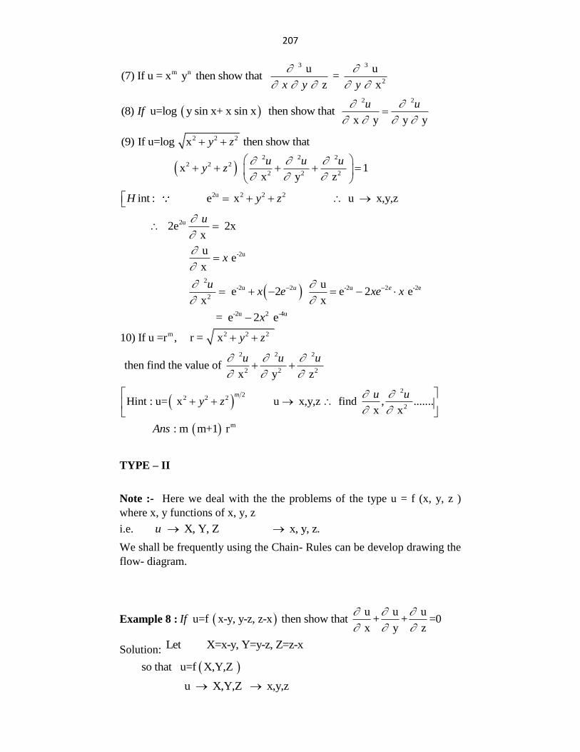
207

m n(7) If u = x y then show that3 3

2

u u =

z xx y y

(8) u=log y sin x+ x sin x then show that If2 2

x y y y

u u

2 2 2(9) If u=log x then show thaty z

2 2 2

2 2 2

2 2 2

x 1

x y z

u u uy z

2u 2 2 2int : e x u x,y,zH y z

2u 2e 2x

x

u

-2u u e

x x

2

-2u 2 -2u 2 -2e

2

u e 2 e 2 e

x x

u eux e xe x

-2u 2 -4u = e 2 e x

m 2 2 210) If u =r , r = x y z

2 2 2

2 2 2

then find the value of

x y z

u u u

2

22 2 2

2

Hint : u= x u x,y,z find , .......

x x

m u uy z

m : m m+1 rAns

TYPE – II

Note :- Here we deal with the the problems of the type u = f (x, y, z )

where x, y functions of x, y, z

i.e. X, Y, Z x, y, z.u

We shall be frequently using the Chain- Rules can be develop drawing the

flow- diagram.

Example 8 : u u u

u=f x-y, y-z, z-x then show that + + =0 x y z

If

Solution: Let X=x-y, Y=y-z, Z=z-x

so that u=f X,Y,Z

u X,Y,Z x,y,z

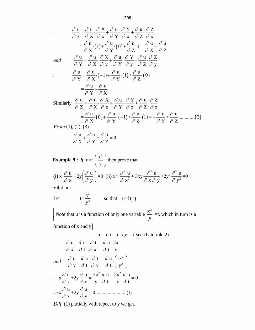
208

u u X u Y u Z = + +

x X x Y x Z x

u u u u u

= 1 + 0 + -1= X Y Z X Z

u u X u Y u Z +

Y X y Y y Z yand

u u u u

1 1 + 0 Y X Y Z

u u =

Y X

u u X u Y u ZSimilarly +

Z X z Y z Z z

u u u u u

= 0 1 + 1 + ............. 3 X Y Z Y Z

(1), (2), (3)From

u u u + 0

X Y Z

Example 9 : 2x

u=f then prove thaty

If

2 2 22 2

2 2

u u u u u(i) x + 2y =0 (ii) x + 3xy +2y =0

x y x x y y

Solution:

2

2Let t= so that u=f t

x

y

2x that u is a function of only one variable =t, which in turn is a Note

y

function of x and y

u t x,y ( see chain rule 2)

u u t u 2x = =

x t x t y

d d

d d

2

2

u u t u -x, = =

y t y t y

d dand

d d

2 2 u u 2 u 2x u x +2y 0

x y t y t

x d d

y d d

u u. .x +2y 0.........................(1)

x yi e

(1) partially with repect to y we get,Diff

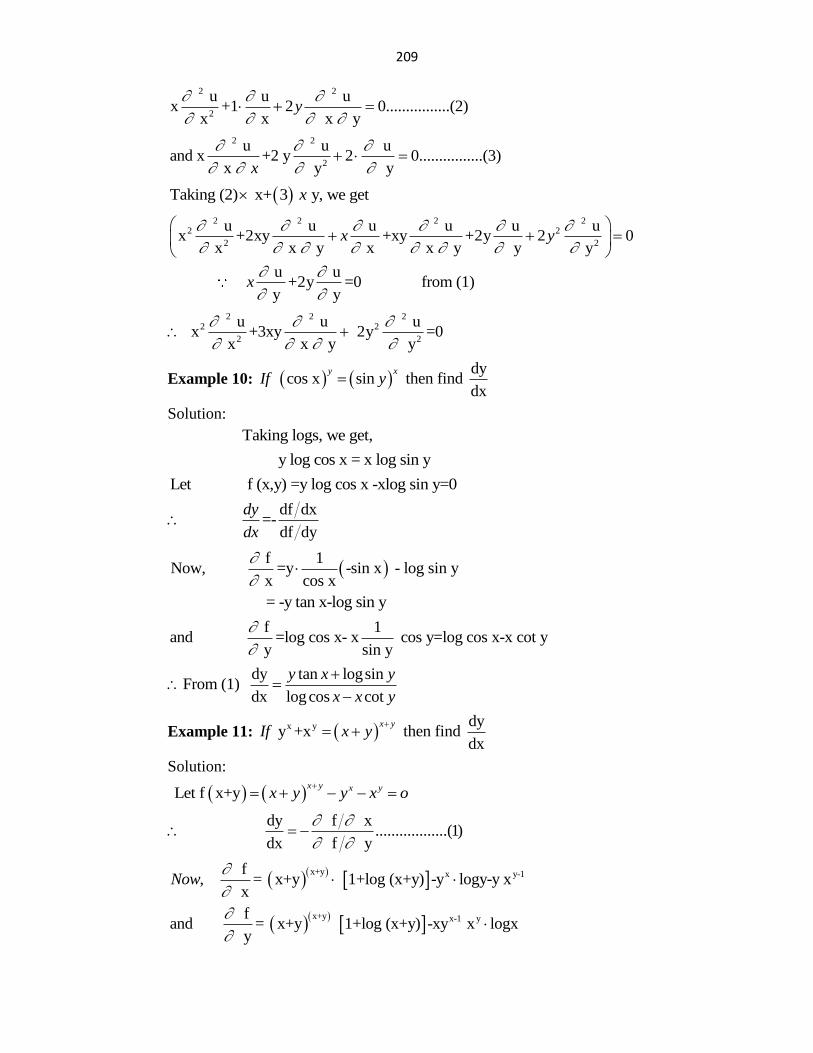
209

2 2

2

u u ux +1 2 0................(2)

x x x yy

2 2

2

u u uand x +2 y 2 0................(3)

x y yx

Taking (2) x+ 3 y, we getx

2 2 2 22 2

2 2

u u u u u ux +2xy +xy +2y 2 0

x x y x x y y yx y

u u

+2y =0 from (1) y y

x

2 2 22 2

2 2

u u u x +3xy 2y =0

x x y y

Example 10: dy

cos x sin then find dx

y xIf y

Solution:

Taking logs, we get,

y log cos x = x log sin y

Let f (x,y) =y log cos x -xlog sin y=0

df dx =-

df dy

dy

dx

f 1

Now, =y -sin x - log sin y x cos x

= -y tan x-log sin y

f 1and =log cos x- x cos y=log cos x-x cot y

y sin y

dy tan logsinFrom (1)

dx logcos cot

y x y

x x y

Example 11: x y dy y +x then find

dx

x yIf x y

Solution:

Let f x+yx y x yx y y x o

dy f x ..................(1)

dx f y

x+y x y-1 f

, = x+y 1+log (x+y) -y logy-y x x

Now

x+y x-1 y f

and = x+y 1+log (x+y) -xy x logx y

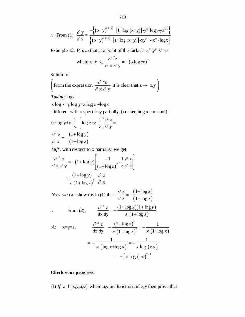
210

x+y x y-1

x+y x-1 y

x+y 1+log (x+y) -y logy-yx y From (1), =

x x+y 1+log (x+y) -xy - x logx

d

d

Example 12: Pr that at a point of the surface ove x y zx y z =c

21

where x=y=z, log y

zx ex

x

Solution: 2

From the expression it is clear that z x,y x y

z

logs Taking

x log x+y log y+z log z =log c

Different with respect to y partially, (i.e. keeping x constant)

1 1 z0+log y+y log z+z

y z y

2 1 log z

x 1 log

y

z

. with respect to x partially, we get,Diff

2

2

z 1 1 z1 log

x y x1 logy

zz

2

1 log z =

x 1 log

y

z z

1 log z, can show (as in (1) that

x 1 log

xNow we

z

2 1 log 1 log z From (2),

x y 1 log

x y

d d z z

2 2

3

1 log z 1 x=y=z,

x y 1+log x 1 log

xAt

d d xx x

1 1

= = log e+log x log e xx x

1

= log exx


(1) z=f x,y,u,v where u,v are functions of x,y then prove that If

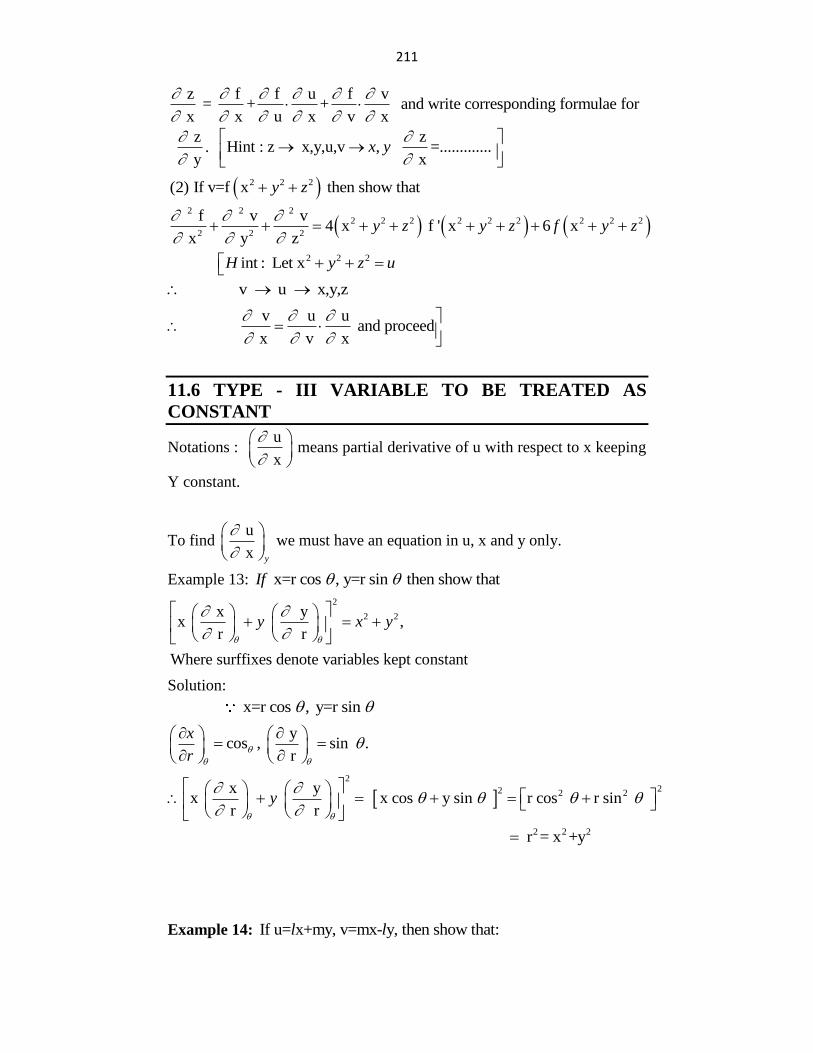
211

z f f u f v = + + and write corresponding formulae for

x x u x v x

z

y

.

zHint : z x,y,u,v , =.............

xx y

2 2 2(2) If v=f x then show that y z

2 2 2

2 2 2 2 2 2 2 2 2

2 2 2

f v v4 x f ' x 6 x

x y zy z y z f y z

2 2 2int : Let x H y z u

v u x,y,z

v u u and proceed

x v x

11.6 TYPE - III VARIABLE TO BE TREATED AS

CONSTANT

Notations : u

x

means partial derivative of u with respect to x keeping

Y constant.

To find u

x y

we must have an equation in u, x and y only.

Example 13: x=r cos , y=r sin then show that If

2

2 2 x yx ,

r r

Where surffixes denote variables kept constant

y x y

Solution:

x=r cos , y=r sin

ycos , sin .

r

x

r

2

22 2 2 x yx x cos y sin r cos r sin

r ry

2 2 2 r = x +y

Example 14: If u= x+my, v=mx- y, then show that:l l

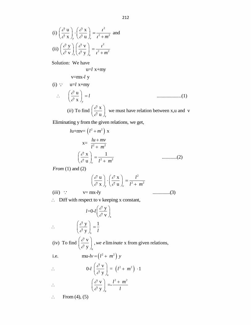
212

2

2 2

u x(i) and

x uy v m

2

2 2

y v(ii)

v yx um

Solution: We have

u= x+myl

v=mx- yl

(i) u= x+myl

u ....................(1)

x y

l

v

x( ) To find we must have relation between x,u and v

uii

Eliminating y from the given relations, we get,

2 2 u+mv= xl l m

2 2 x=

lu mv

l m

2 2

v

x 1 ............(2)

u l m

(1) and (2) From

2

2 2

y v

u x

x u

l

l m

( ) v= mx- y ..............(3)iii l

Diff with respect to v keeping x constant,

x

y =0-

vl l

x

y 1

y l

u

v(iv) To find , lim x from given relations,

ywe e inate

2 2i.e. mu- lv l m y

2 2

u

v 0- = 1

yl l m

2 2

u

v =-

y

l m

l

From (4), (5)

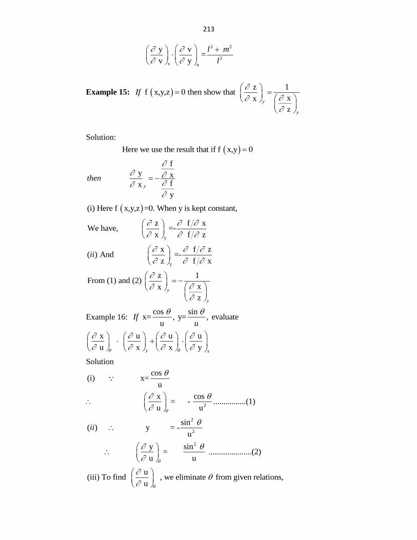
213

2 2

2

x u

y v =

v y

l m

l

Example 15: f x,y,z 0 then show that If z 1

x x

zy

y

Solution:

Here we use the result that if f x,y 0

f

y x f x

y

y

then

(i) Here f x,y,z =0. When y is kept constant,

y

z f xWe have, =-

x f z

y

x f z( ) And =-

z f xii

z 1From (1) and (2)

x x

zy

y

Example 16: cos sin

x= , y= , evaluateu

Ifu

x u u u

u x x yy x

Solution

cos (i) x=

u

2

x cos = - ................(1)

u u

2

2

sin ( ) y = -

uii

2 y sin = .....................(2)

u u

u(iii) To find , we eliminate from given relations,

u

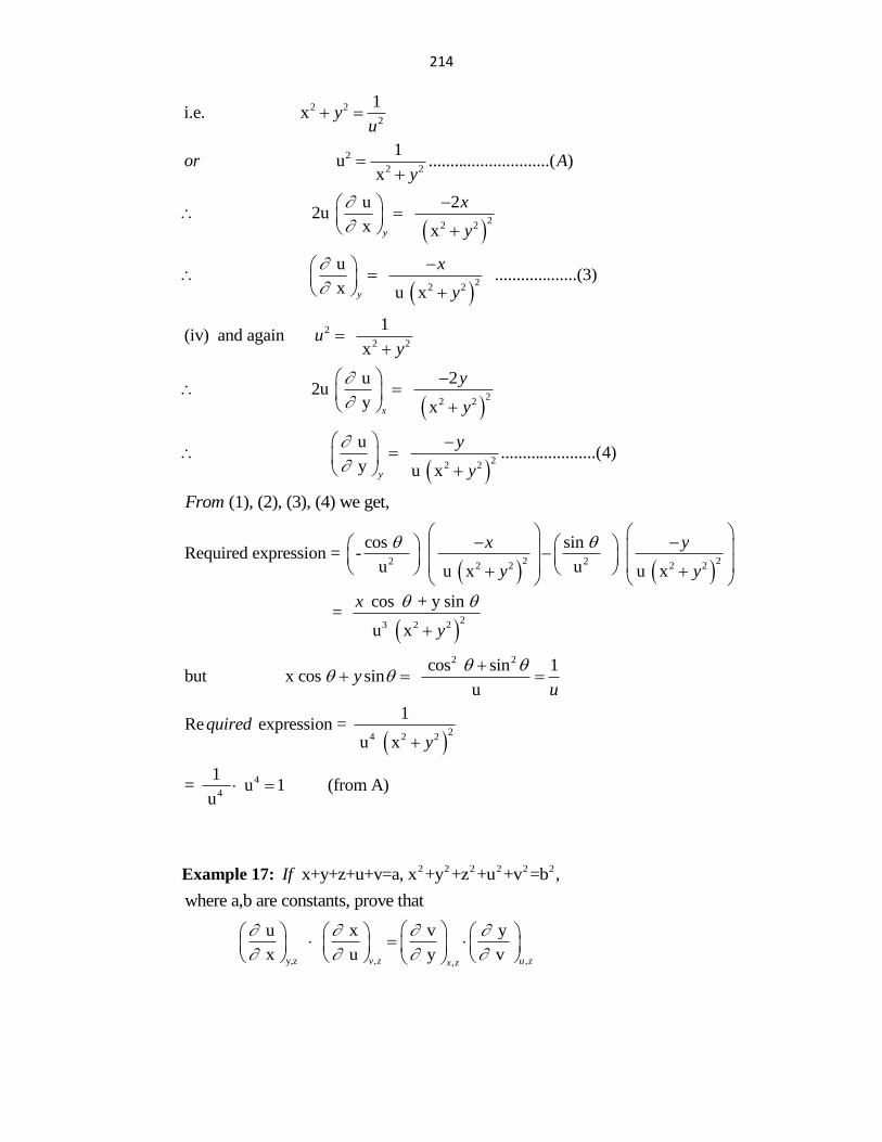
214

2 2

2

1i.e. x y

u

2

2 2

1 u ............................( )

xor A

y

2

2 2

u 2 2u

x xy

x

y

2

2 2

u ...................(3)

x u xy

x

y

2

2 2

1(iv) and again

xu

y

2

2 2

u 2 2u

y xx

y

y

2

2 2

u ......................(4)

y u xy

y

y

(1), (2), (3), (4) we get,From

2 22 22 2 2 2

cos sin Required expression = -

u u u x u x

x y

y y

2

3 2 2

cos + y sin =

u x

x

y

2 2 cos sin 1but x cos sin

uy

u

2

4 2 2

1Re expression =

u xquired

y

4

4

1= u 1 (from A)

u

Example 17: 2 2 2 2 2 2 x+y+z+u+v=a, x +y +z +u +v =b , If

where a,b are constants, prove that

y,z , ,,

u x v y

x u y v v z u zx z

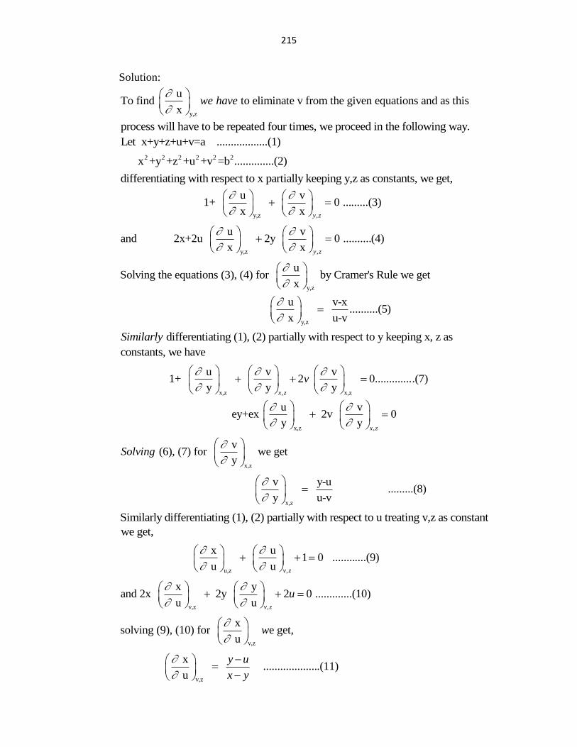
215

Solution:

y,z

uTo find to eliminate v from the given equations and as this

xwe have

process will have to be repeated four times, we proceed in the following way.

Let x+y+z+u+v=a ..................(1)

2 2 2 2 2 2 x +y +z +u +v =b ..............(2)

differentiating with respect to x partially keeping y,z as constants, we get,

y,z ,

u v 1+ 0 .........(3)

x x y z

y,z ,

u vand 2x+2u 2y 0 ..........(4)

x x y z

y,z

uSolving the equations (3), (4) for by Cramer's Rule we get

x

y,z

u v-x ..........(5)

x u-v

differentiating (1), (2) partially with respect to y keeping x, z as Similarly

constants, we have

x,z , x,z

u v v 1+ 2 0..............(7)

y y yx z

v

x,z ,

u v ey+ex 2v 0

y yx z

x,z

v (6), (7) for we get

ySolving

x,z

v y-u .........(8)

y u-v

Similarly differentiating (1), (2) partially with respect to u treating v,z as constant

we get,

u,z ,

x u 1 0 ............(9)

u u v z

v,z ,

x yand 2x 2y 2 0 .............(10)

u u v z

u

v,z

xsolving (9), (10) for e get,

uw

v,z

x ....................(11)

u

y u

x y

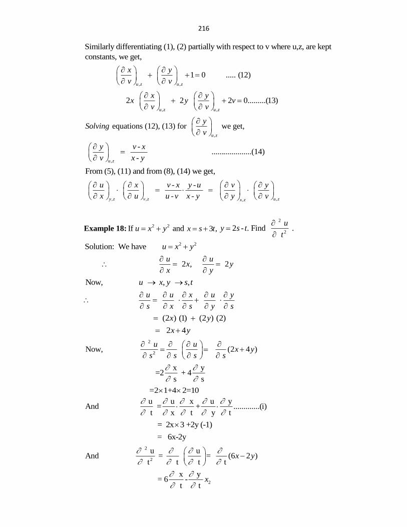
216

Similarly differentiating (1), (2) partially with respect to v where u,z, are kept

constants, we get,

, ,

1 0 ..... (12)

u z u z

x y

v v

, ,

2 2 2 0.........(13)

u z u z

x yx y v

v v

,

equations (12), (13) for we get,

u z

ySolving

v

,

- ....................(14)

- u z

y v x

v x y

From (5), (11) and from (8), (14) we get,

, , ,,

- -

- - y z v z u zx z

u x v x y u v y

x u u v x y y v

Example 18:2 2If andu x y 3 ,x s t

2

2

2 - . Find .

uy s t

t

2 2Solution: We have u x y

2 , 2

u ux y

x y

Now, , ,u x y s t

u u x u y

s x s y s

(2 ) (1) (2 ) (2) x y

2 4x y

2

2

Now, (2 4 )

u ux y

s s s s

x y =2 + 4

s s

=2 1+4 2=10

u u x u yAnd = + .............(i)

t x t y t

= 2x 3 +2y (-1)

= 6x-2y

2

2

u u And = = (6 2 )

t t t tx y

2

x y = 6 -

t tx

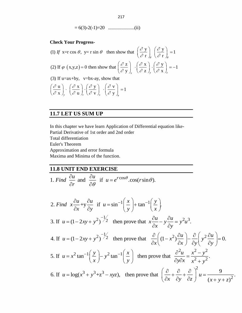
217

= 6(3)-2(-1)=20 ......................(ii)

Check Your Progress-

y y(1) x=r cos , y= r sin then show that 1

r rIf

z x y

(2) If x,y,z 0 then show that 1 y z xy zx

(3) If u=ax+by, v=bx-ay, show that

u x y v 1

x u v yy v x u

11.7 LET US SUM UP

In this chapter we have learn Application of Differential equation like-

Partial Derivative of 1st order and 2nd order

Total differentiation

Euler's Theorem

Approximation and error formula

Maxima and Minima of the function.


cos1. and if .cos( sin ).ru uFind u e r

r

1 12. +y if sin tan .u u x y

Find x ux y y x

12 2 323. If (1 2 ) then prove that .

u uu xy y x y y u

x y

12 2 224. If (1 2 ) then prove that (1 ) 0.

u uu xy y x y

x x y y

2 2 2

2 1 2 1

2 25. If tan tan then prove that .

y x u x yu x y

x y y x x y

2

3 3 3

2

96. If log( +z ), then prove that .

( )u x y xyz u

x y z x y z

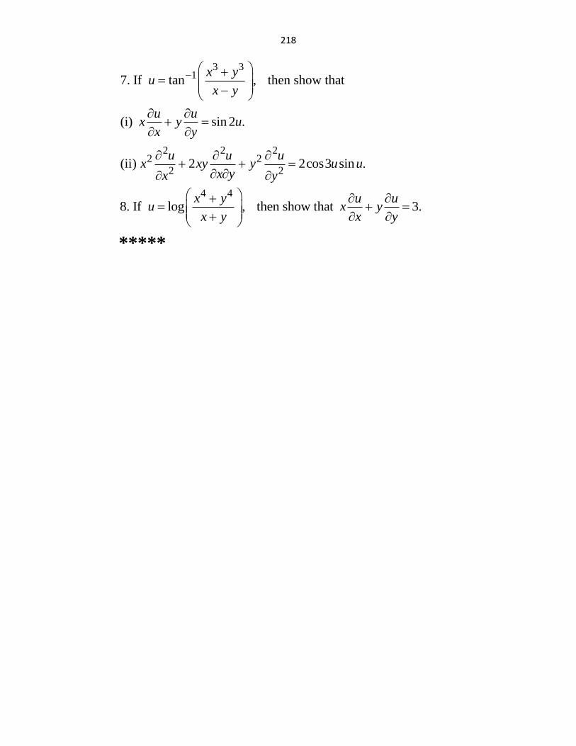
218

3 31

2 2 22 2

2 2

7. If tan , then show that

(i) sin 2 .

(ii) 2 2cos3 sin .

x yu

x y

u ux y u

x y

u u ux xy y u u

x yx y

4 4

8. If log , then show that 3.x y u u

u x yx y x y

*****

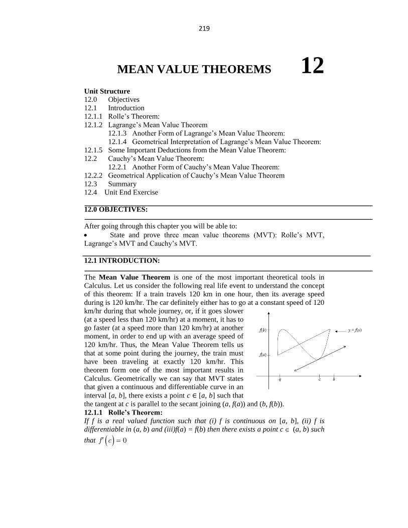
219

MEAN VALUE THEOREMS 12

Unit Structure

12.0 Objectives

12.1 Introduction

12.1.1 Rolle‟s Theorem:

12.1.2 Lagrange‟s Mean Value Theorem

12.1.3 Another Form of Lagrange‟s Mean Value Theorem:

12.1.4 Geometrical Interpretation of Lagrange‟s Mean Value Theorem:

12.1.5 Some Important Deductions from the Mean Value Theorem:

12.2 Cauchy‟s Mean Value Theorem:

12.2.1 Another Form of Cauchy‟s Mean Value Theorem:

12.2.2 Geometrical Application of Cauchy‟s Mean Value Theorem

12.3 Summary


12.0 OBJECTIVES:

After going through this chapter you will be able to:

State and prove three mean value theorems (MVT): Rolle‟s MVT,

Lagrange‟s MVT and Cauchy‟s MVT.

12.1 INTRODUCTION:

The Mean Value Theorem is one of the most important theoretical tools in

Calculus. Let us consider the following real life event to understand the concept

of this theorem: If a train travels 120 km in one hour, then its average speed

during is 120 km/hr. The car definitely either has to go at a constant speed of 120

km/hr during that whole journey, or, if it goes slower

(at a speed less than 120 km/hr) at a moment, it has to

go faster (at a speed more than 120 km/hr) at another

moment, in order to end up with an average speed of

120 km/hr. Thus, the Mean Value Theorem tells us

that at some point during the journey, the train must

have been traveling at exactly 120 km/hr. This

theorem form one of the most important results in

Calculus. Geometrically we can say that MVT states

that given a continuous and differentiable curve in an

interval [a, b], there exists a point c ∈ [a, b] such that

the tangent at c is parallel to the secant joining (a, f(a)) and (b, f(b)).

12.1.1 Rolle’s Theorem:

If f is a real valued function such that (i) f is continuous on [a, b], (ii) f is

differentiable in (a, b) and (iii)f(a) = f(b) then there exists a point c (a, b) such

that f c 0

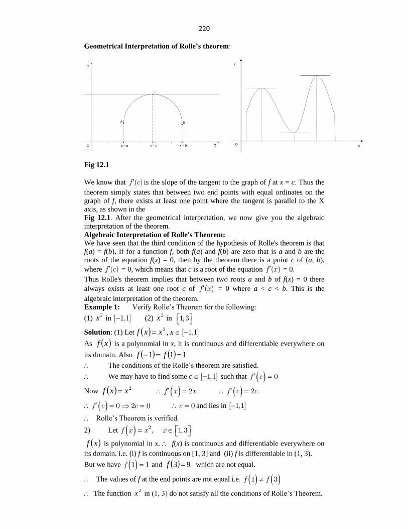
220 Geometrical Interpretation of Rolle’s theorem:

Fig 12.1

We know that f c( ) is the slope of the tangent to the graph of f at x = c. Thus the

theorem simply states that between two end points with equal ordinates on the

graph of f, there exists at least one point where the tangent is parallel to the X

axis, as shown in the

Fig 12.1. After the geometrical interpretation, we now give you the algebraic

interpretation of the theorem.

Algebraic Interpretation of Rolle's Theorem:

We have seen that the third condition of the hypothesis of Rolle's theorem is that

f(a) = f(b). If for a function f, both f(a) and f(b) are zero that is a and b are the

roots of the equation f(x) = 0, then by the theorem there is a point c of (a, b),

where f c( ) = 0, which means that c is a root of the equation f x( ) = 0.

Thus Rolle's theorem implies that between two roots a and b of f(x) = 0 there

always exists at least one root c of f x( ) = 0 where a < c < b. This is the

algebraic interpretation of the theorem.

Example 1: Verify Rolle‟s Theorem for the following:

(1) 2x in [ 1,1] (2)

2x in 1, 3

Solution: (1) Let 2xxf , x [ 1,1]

As xf is a polynomial in x, it is continuous and differentiable everywhere on

its domain. Also 111 ff

The conditions of the Rolle‟s theorem are satisfied.

We may have to find some c [ 1,1] such that f c 0

Now 2xxf f x x2 . f c c2 .

f c c0 2 0 c 0 and lies in [ 1,1]

Rolle‟s Theorem is verified.

2) Let f x x2, x 1, 3

xf is polynomial in x. f(x) is continuous and differentiable everywhere on

its domain. i.e. (i) f is continuous on [1, 3] and (ii) f is differentiable in (1, 3).

But we have f 1 1 and 3f 9 which are not equal.

The values of f at the end points are not equal i.e. f f1 3

The function 2x in (1, 3) do not satisfy all the conditions of Rolle‟s Theorem.

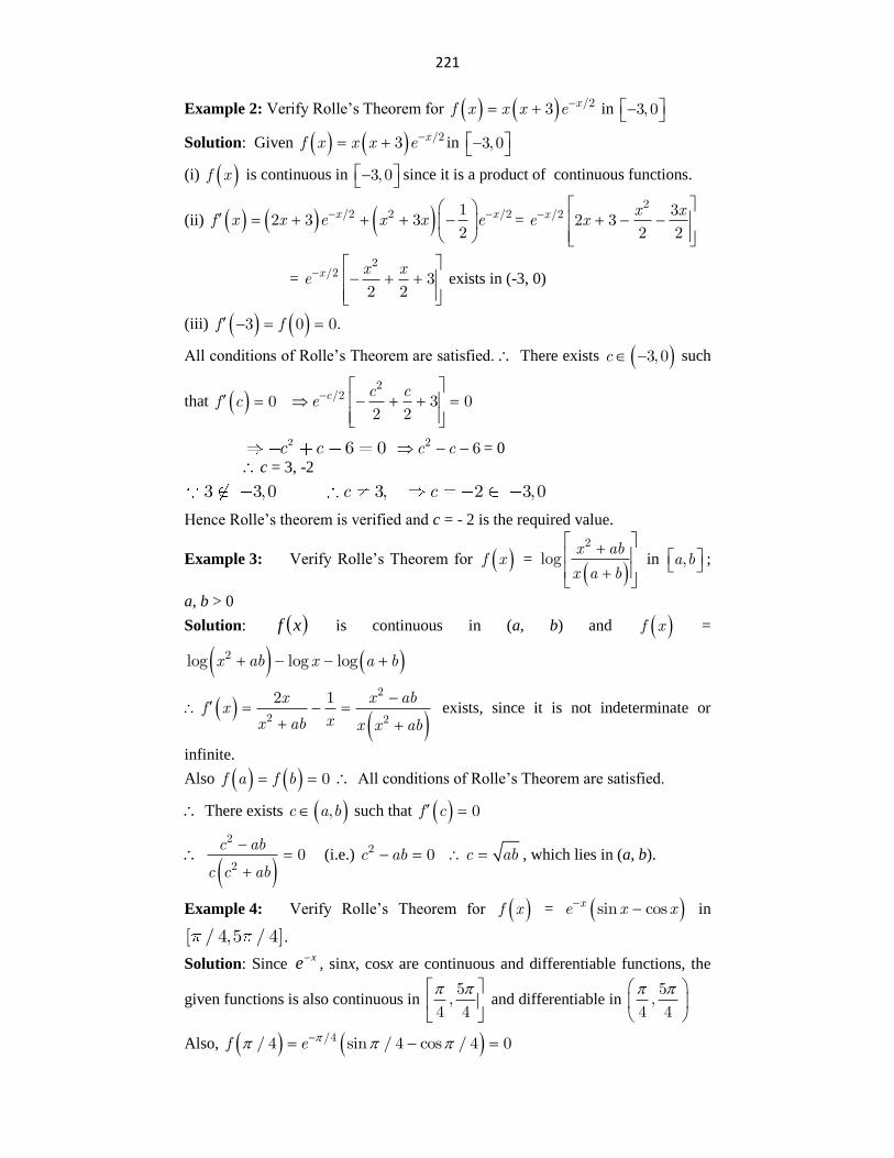
221

Example 2: Verify Rolle‟s Theorem for xf x x x e /23 in 3, 0

Solution: Given xf x x x e /23 in 3, 0

(i) f x is continuous in 3, 0 since it is a product of continuous functions.

(ii) x xf x x e x x e/2 2 /212 3 3

2

= x x xe x

2/2 3

2 32 2

= x x xe

2/2 3

2 2

exists in (-3, 0)

(iii) f f3 0 0.

All conditions of Rolle‟s Theorem are satisfied. There exists c 3, 0 such

that f c 0 c c ce

2/2 3 0

2 2

c c2 6 0 c c2 6 = 0

c = 3, -2

c c3 3,0 3, 2 3,0

Hence Rolle‟s theorem is verified and c = - 2 is the required value.

Example 3: Verify Rolle‟s Theorem for f x = x ab

x a b

2

log

in a b, ;

a, b > 0

Solution: xf is continuous in (a, b) and f x =

x ab x a b2log log log

x x abf x

xx ab x x ab

2

2 2

2 1

exists, since it is not indeterminate or

infinite.

Also f a f b 0 All conditions of Rolle‟s Theorem are satisfied.

There exists c a b, such that f c 0

c ab

c c ab

2

20

(i.e.) c ab2 0 c ab , which lies in (a, b).

Example 4: Verify Rolle‟s Theorem for f x = xe x xsin cos in

[ / 4,5 / 4].

Solution: Since xe, sinx, cosx are continuous and differentiable functions, the

given functions is also continuous in 5

,4 4

and differentiable in 5

,4 4

Also, f e /4/ 4 sin / 4 cos / 4 0

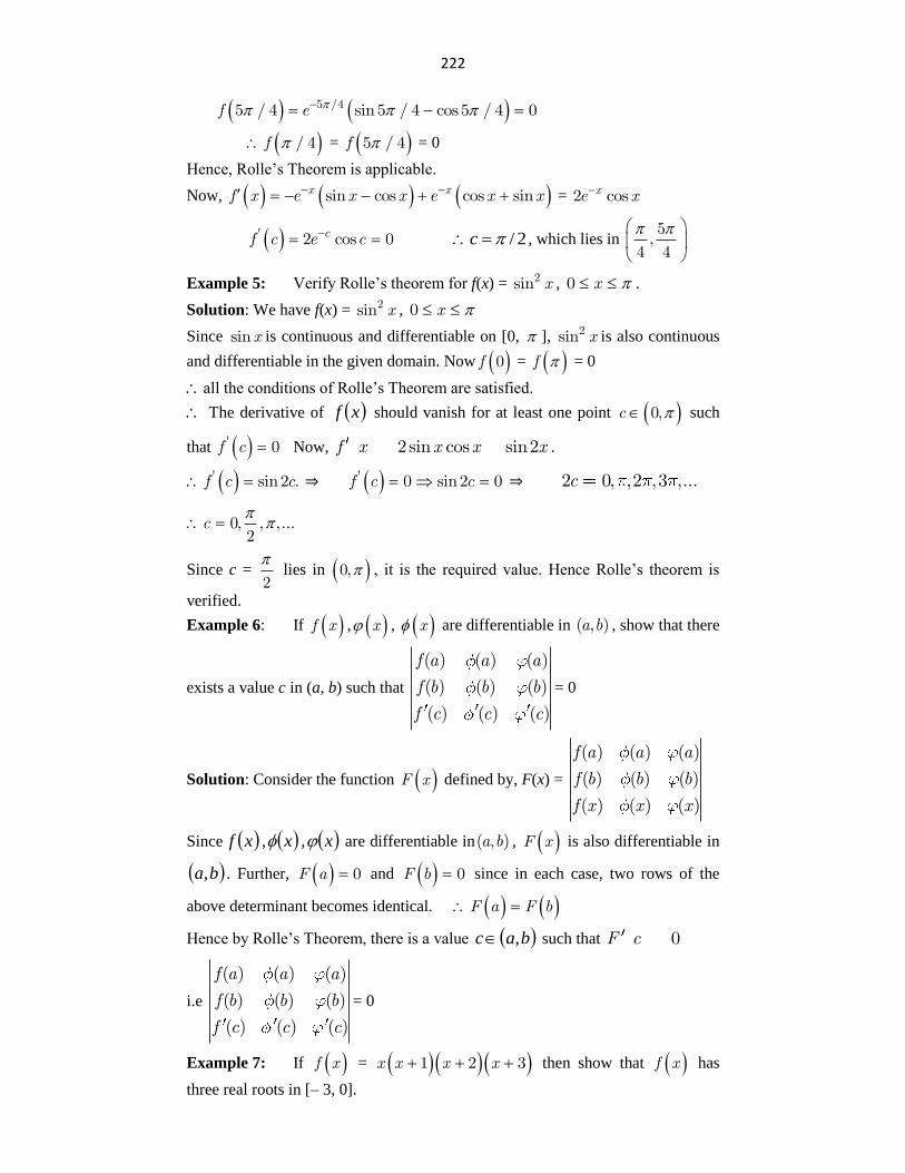
222

f e 5 /45 / 4 sin5 / 4 cos5 / 4 0

f / 4 = f 5 / 4 = 0

Hence, Rolle‟s Theorem is applicable.

Now, x xf x e x x e x xsin cos cos sin = xe x2 cos

cf c e c' 2 cos 0 2/c , which lies in 5

,4 4

Example 5: Verify Rolle‟s theorem for f(x) = x2sin , x0 .

Solution: We have f(x) = x2sin , x0

Since xsin is continuous and differentiable on [0, ], x2sin is also continuous

and differentiable in the given domain. Now f 0 = f = 0

all the conditions of Rolle‟s Theorem are satisfied.

The derivative of xf should vanish for at least one point c 0, such

that f c' 0 Now, f x x x x2sin cos sin2 .

f c c' sin2 . ⇒ f c c' 0 sin2 0 ⇒ c2 0, , ,.2 .,3 .

c 0, ,2

,...

Since c = 2

lies in 0, , it is the required value. Hence Rolle‟s theorem is

verified.

Example 6: If f x , x , x are differentiable in a b( , ) , show that there

exists a value c in (a, b) such that

f a a a

f b b b

f c c c

( ) ( ) ( )

( ) ( ) ( )

( ) ( ) ( )

= 0

Solution: Consider the function F x defined by, F(x) =

( ) ( ) ( )

( ) ( ) ( )

( ) ( ) ( )

f a a a

f b b b

f x x x

Since xf , x , x are differentiable in a b( , ) , F x is also differentiable in

ba, . Further, F a 0 and F b 0 since in each case, two rows of the

above determinant becomes identical. F a F b

Hence by Rolle‟s Theorem, there is a value bac , such that F c 0

i.e

f a a a

f b b b

f c c c

( ) ( ) ( )

( ) ( ) ( )

( ) ( ) ( )

= 0

Example 7: If f x = x x x x1 2 3 then show that f x has

three real roots in [– 3, 0].

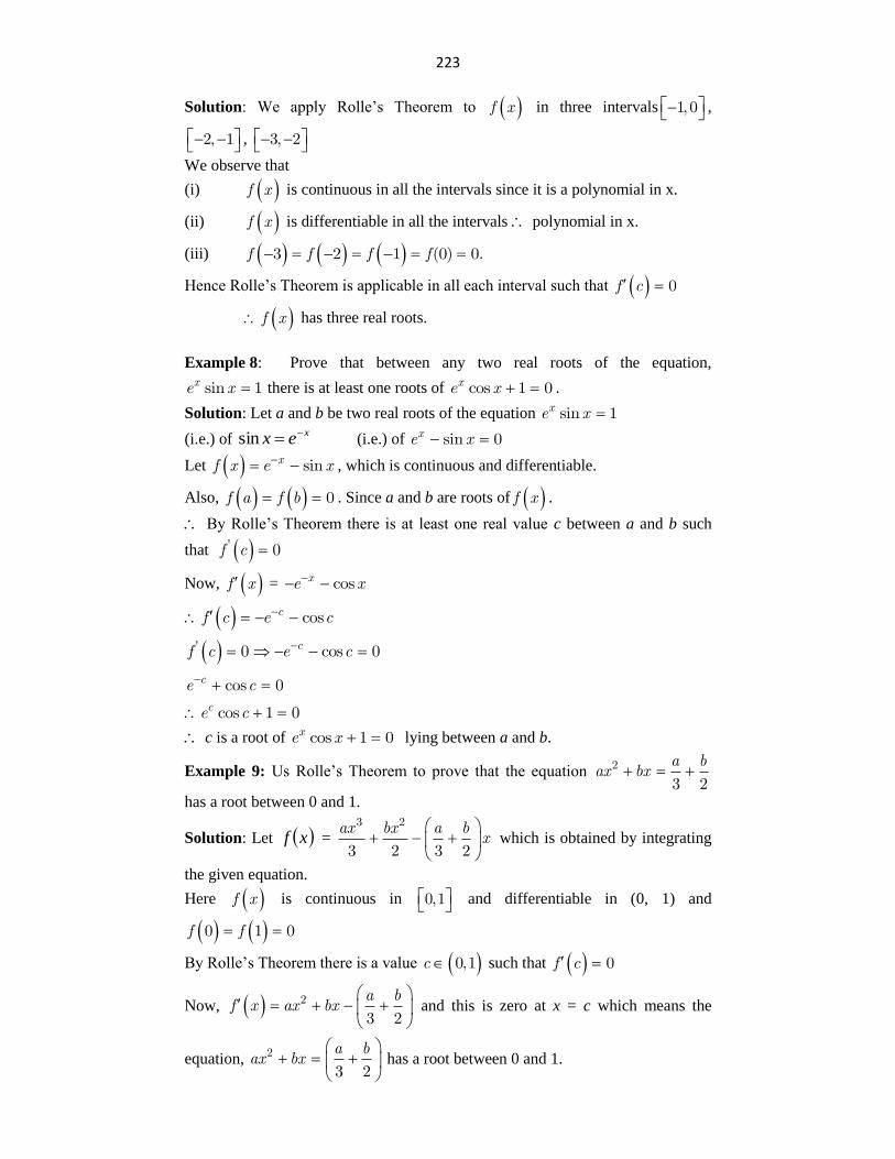
223

Solution: We apply Rolle‟s Theorem to f x in three intervals 1, 0 ,

2, 1 , 3, 2

We observe that

(i) f x is continuous in all the intervals since it is a polynomial in x.

(ii) f x is differentiable in all the intervals polynomial in x.

(iii) f f f f3 2 1 (0) 0.

Hence Rolle‟s Theorem is applicable in all each interval such that f c 0

f x has three real roots.

Example 8: Prove that between any two real roots of the equation, xe xsin 1 there is at least one roots of xe xcos 1 0 .

Solution: Let a and b be two real roots of the equation xe xsin 1

(i.e.) of xex sin (i.e.) of xe xsin 0

Let xf x e xsin , which is continuous and differentiable.

Also, f a f b 0 . Since a and b are roots of f x .

By Rolle‟s Theorem there is at least one real value c between a and b such

that f c' 0

Now, f x = xe xcos

cf c e ccos

cf c e c' 0 cos 0

c

c

e c

e c

cos 0

cos 1 0

c is a root of xe xcos 1 0 lying between a and b.

Example 9: Us Rolle‟s Theorem to prove that the equation a b

ax bx2

3 2

has a root between 0 and 1.

Solution: Let xf = ax bx a b

x3 2

3 2 3 2

which is obtained by integrating

the given equation.

Here f x is continuous in 0,1 and differentiable in (0, 1) and

f f0 1 0

By Rolle‟s Theorem there is a value c 0,1 such that f c 0

Now, a b

f x ax bx2

3 2

and this is zero at x = c which means the

equation, a b

ax bx2

3 2

has a root between 0 and 1.

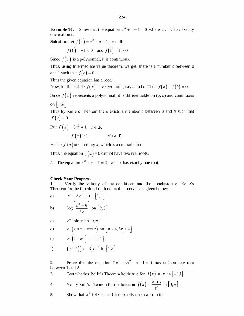
224

Example 10: Show that the equation x x3 1 0 where x has exactly

one real root.

Solution: Let f x x x3 1, x

f 0 1 0 and f 1 1 0

Since f x is a polynomial, it is continuous.

Thus, using Intermediate value theorem, we get, there is a number c between 0

and 1 such that f c 0

Thus the given equation has a root.

Now, let if possible f x have two roots, say a and b. Then f a = f b 0 .

Since f x represents a polynomial, it is differentiable on (a, b) and continuous

on a b,

Thus by Rolle‟s Theorem there exists a member c between a and b such that

f c 0

But f x x23 1, x

f x 1 , x

Hence f x 0 for any x, which is a contradiction.

Thus, the equation f x = 0 cannot have two real roots.

The equation x x3 1 0, x has exactly one root.

Check Your Progress

1. Verify the validity of the conditions and the conclusion of Rolle‟s

Theorem for the function f defined on the intervals as given below:

a) x x2 3 2 on 1,2

b) x

x

2 6log

5

on 2, 3

c) xe xsin on [0, ]

d) xe x xsin cos on / 4,5 / 4

e) x x2 21 on 0,1

f) xx x e1 3 in 1, 3

2. Prove that the equation x x x3 22 3 1 0 has at least one root

between 1 and 2.

3. Test whether Rolle‟s Theorem holds true for xf = x in 1,1

4. Verify Roll‟s Theorem for the function xf = xe

xsin in ,0

5. Show that 0143 xx has exactly one real solution.

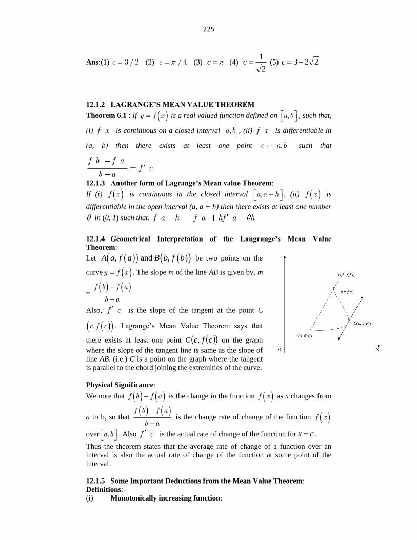
225

Ans:(1) c 3 / 2 (2) c / 4 (3) c (4) 2

1c (5) 223c

12.1.2 LAGRANGE’S MEAN VALUE THEOREM

Theorem 6.1 : If y f x is a real valued function defined on a b, , such that,

(i) f x is continuous on a closed interval ,a b , (ii) f x is differentiable in

(a, b) then there exists at least one point ,c a b such that

f b f af c

b a

12.1.3 Another form of Lagrange’s Mean value Theorem:

If (i) f x is continuous in the closed interval a a h, , (ii) f x is

differentiable in the open interval (a, a + h) then there exists at least one number

in (0, 1) such that, f a h f a hf a h

12.1.4 Geometrical Interpretation of the Langrange’s Mean Value

Theorem:

Let , and ,A a f a B b f b be two points on the

curve y f x . The slope m of the line AB is given by, m

= f b f a

b a

Also, f c is the slope of the tangent at the point C

c f c, . Lagrange‟s Mean Value Theorem says that

there exists at least one point C cfc, on the graph

where the slope of the tangent line is same as the slope of

line AB. (i.e.) C is a point on the graph where the tangent

is parallel to the chord joining the extremities of the curve.

Physical Significance:

We note that f b f a is the change in the function f x as x changes from

a to b, so that f b f a

b a

is the change rate of change of the function f x

over a b, . Also f c is the actual rate of change of the function for cx .

Thus the theorem states that the average rate of change of a function over an

interval is also the actual rate of change of the function at some point of the

interval.

12.1.5 Some Important Deductions from the Mean Value Theorem:

Definitions:-

(i) Monotonically increasing function:

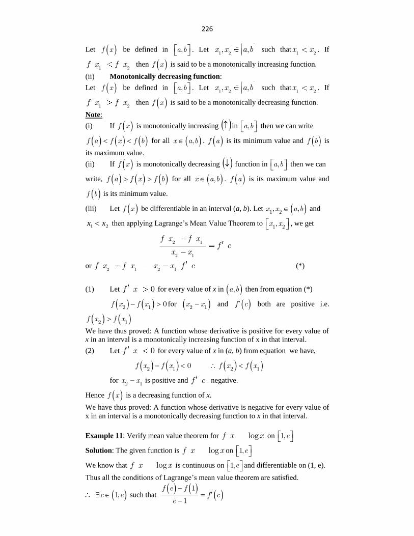
226

Let f x be defined in a b, . Let

1 2, ,x x a b such that

1 2x x . If

1 2f x f x then f x is said to be a monotonically increasing function.

(ii) Monotonically decreasing function:

Let f x be defined in a b, . Let

1 2, ,x x a b such that

1 2x x . If

f x f x1 2

then f x is said to be a monotonically decreasing function.

Note:

(i) If f x is monotonically increasing in a b, then we can write

f a f x f b for all x a b, . f a is its minimum value and f b is

its maximum value.

(ii) If f x is monotonically decreasing function in a b, then we can

write, f a f x f b for all x a b, . f a is its maximum value and

f b is its minimum value.

(iii) Let f x be differentiable in an interval (a, b). Let x x a b1 2, , and

21 xx then applying Lagrange‟s Mean Value Theorem to x x1 2, , we get

2 1

2 1

f x f xf c

x x

or 2 1 2 1

f x f x x x f c (*)

(1) Let 0f x for every value of x in a b, then from equation (*)

f x f x2 1 0 for x x2 1 and f c both are positive i.e.

f x f x2 1

We have thus proved: A function whose derivative is positive for every value of

x in an interval is a monotonically increasing function of x in that interval.

(2) Let 0f x for every value of x in (a, b) from equation we have,

f x f x2 1 0 f x f x2 1

for x x2 1 is positive and f c negative.

Hence f x is a decreasing function of x.

We have thus proved: A function whose derivative is negative for every value of

x in an interval is a monotonically decreasing function to x in that interval.

Example 11: Verify mean value theorem for logf x x on e1,

Solution: The given function is logf x x on e1,

We know that logf x x is continuous on e1, and differentiable on (1, e).

Thus all the conditions of Lagrange‟s mean value theorem are satisfied.

c e1, such that

f e f

f ce

1

1

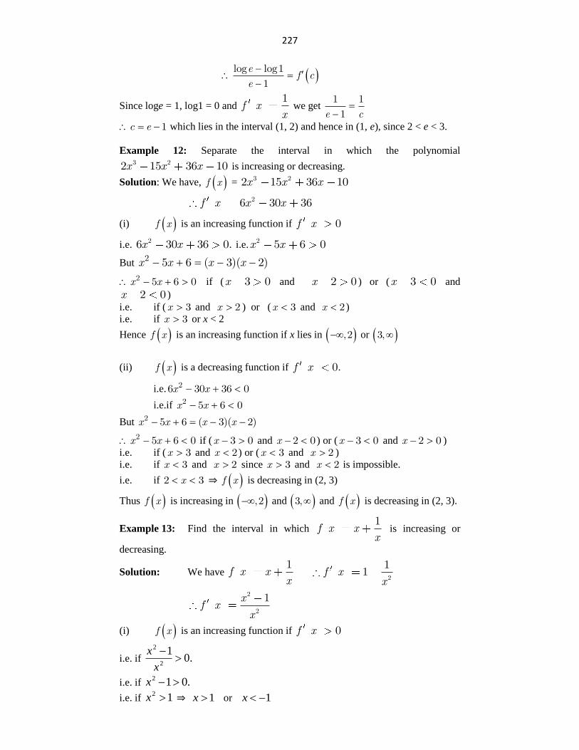
227

e

f ce

log log1

1

Since loge = 1, log1 = 0 and 1

f xx

we get e c

1 1

1

c e 1 which lies in the interval (1, 2) and hence in (1, e), since 2 < e < 3.

Example 12: Separate the interval in which the polynomial

x x x3 22 15 36 10 is increasing or decreasing.

Solution: We have, f x = x x x3 22 15 36 10

26 30 36f x x x

(i) f x is an increasing function if 0f x

i.e. 26 30 36 0.x x i.e.

2 5 6 0x x

But x x x x2 5 6 ( 3)( 2)

x x2 5 6 0 if ( 3 0x and x 2 0 ) or (x 3 0 and

x 2 0 )

i.e. if (x 3 and x 2 ) or (x 3 and x 2 )

i.e. if x 3 or x < 2

Hence f x is an increasing function if x lies in ,2 or 3,

(ii) f x is a decreasing function if 0.f x

i.e. x x26 30 36 0

i.e.if x x2 5 6 0

But x x x x2 5 6 ( 3)( 2)

x x2 5 6 0 if (x 3 0 and x 2 0 ) or (x 3 0 and x 2 0 )

i.e. if (x 3 and x 2 ) or (x 3 and x 2 )

i.e. if x 3 and x 2 since x 3 and x 2 is impossible.

i.e. if x2 3 ⇒ f x is decreasing in (2, 3)

Thus f x is increasing in ,2 and 3, and f x is decreasing in (2, 3).

Example 13: Find the interval in which 1

f x xx

is increasing or

decreasing.

Solution: We have 1

f x xx

2

11f xx

2

2

1xf x

x

(i) f x is an increasing function if 0f x

i.e. if .01

2

2

x

x

i.e. if .012 x

i.e. if 12 x ⇒ 1x or 1x

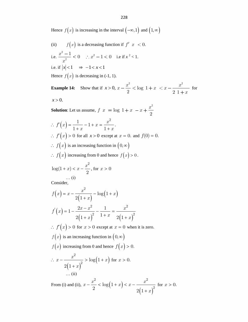
228

Hence f x is increasing in the interval ,1 and 1,

(ii) f x is a decreasing function if 0.f x

i.e.

2

2

10

x

x

2 1 0x i.e if x 2 < 1.

i.e. if 1x ⇒ 11 x

Hence f x is decreasing in (-1, 1).

Example 14: Show that if ,0x2 2

log 12 2 1

x xx x x

x for

.0x

Solution: Let us assume,

2

log 12

xf x x x

x

f x xx x

211 .

1 1

f x 0 for all 0x except at x 0. and f(0) 0.

f x is an increasing function in 0,

f x increasing from 0 and hence f x 0 .

xx x

2

log(1 )2

, for x 0

… (i)

Consider,

x

f x x xx

2

log 12 1

x x xf x

xx x

2 2'

2 2

2 11

12 1 2 1

f x 0 for x 0 except at x 0 when it is zero.

f x is an increasing function in 0,

f x increasing from 0 and hence f x 0.

xx x

x

2

2log 1

2 1

for x 0.

… (ii)

From (i) and (ii),

x xx x x

x

2 2

2log 1

2 2 1

for x 0.

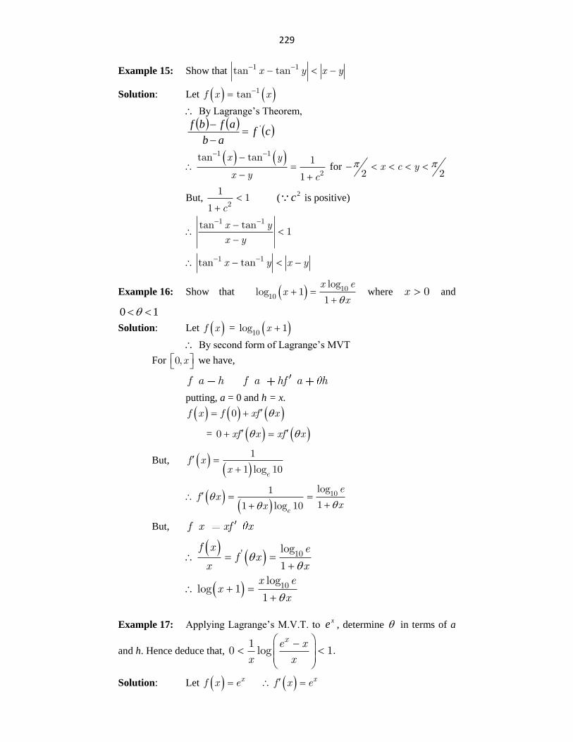
229

Example 15: Show that x y x y1 1tan tan

Solution: Let f x x1tan

By Lagrange‟s Theorem,

cfab

afbf '

x y

x y c

1 1

2

tan tan 1

1

for x c y

2 2

But, c2

11

1

(

2c is positive)

x y

x y

1 1tan tan1

x y x y1 1tan tan

Example 16: Show that x e

xx

1010

loglog 1

1

where x 0 and

10

Solution: Let f x = x10log 1

By second form of Lagrange‟s MVT

For x0, we have,

f a h f a hf a h

putting, a = 0 and h = x.

f x f xf x0

= xf x xf x0

But, e

f xx

1

1 log 10

e

ef x

xx10log1

11 log 10

But, f x xf x

f x e

f xx x

' 10log

1

x e

xx

10loglog 1

1

Example 17: Applying Lagrange‟s M.V.T. to xe , determine in terms of a

and h. Hence deduce that,

xe x

x x

10 log 1.

Solution: Let xf x e xf x e

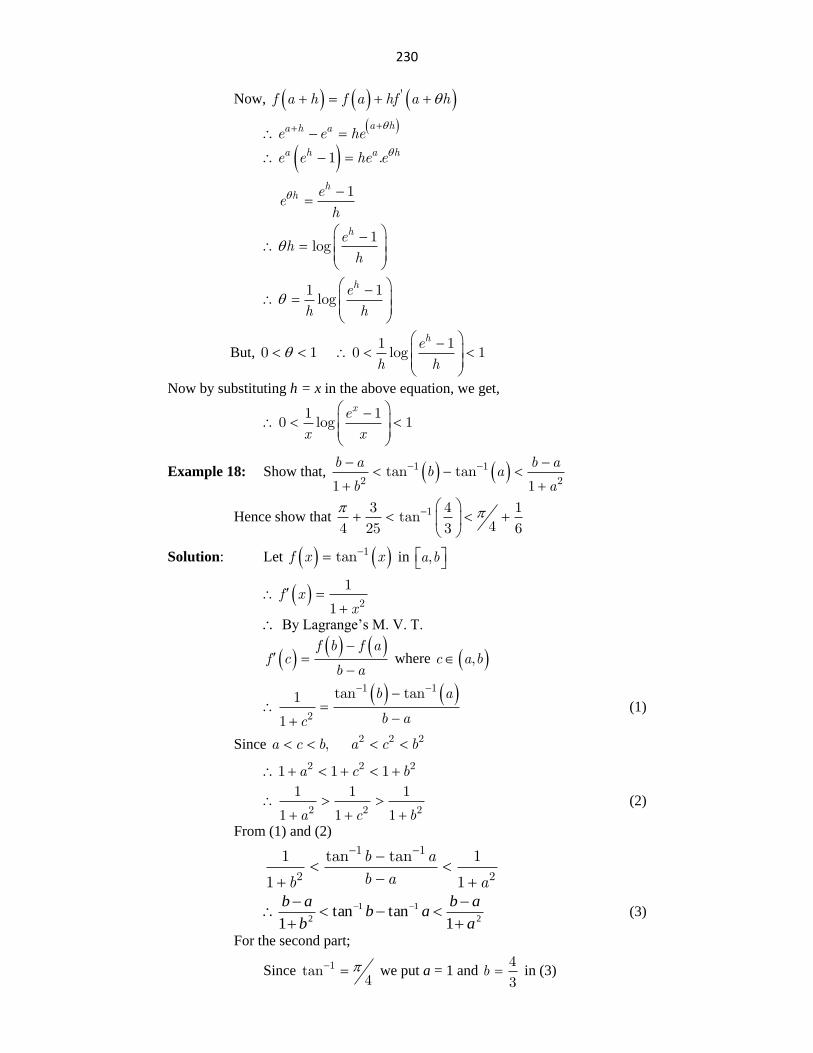
230

Now, f a h f a hf a h'

a ha h ae e he

a h a he e he e1 .

h

h ee

h

1

he

hh

1log

he

h h

1 1log

But, 0 1 he

h h

1 10 log 1

Now by substituting h = x in the above equation, we get,

xe

x x

1 10 log 1

Example 18: Show that, b a b a

b ab a

1 1

2 2tan tan

1 1

Hence show that 13 4 1tan

44 25 3 6

Solution: Let f x x1tan in a b,

f xx2

1

1

By Lagrange‟s M. V. T.

f b f a

f cb a

where c a b,

b a

b ac

1 1

2

tan tan1

1

(1)

Since a c b, a c b2 2 2

a c b2 2 21 1 1

a c b2 2 2

1 1 1

1 1 1

(2)

From (1) and (2)

b a

b ab a

1 1

2 2

1 tan tan 1

1 1

2

11

2 1tantan

1 a

abab

b

ab

(3)

For the second part;

Since 1tan4

we put a = 1 and b4

3 in (3)

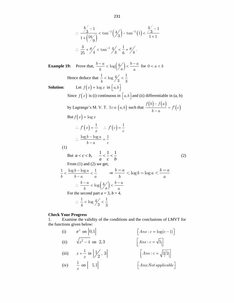
231

1 1

4 41 13 34tan tan 1

3 1 11619

13 14tan .4 3 425 6

Example 19: Prove that, b a b abab a

log

for a b0

Hence deduce that 1 14log

34 3

Solution: Let f x xlog in a b,

Since f x is (i) continuous in a b, and (ii) differentiable in (a, b)

by Lagrange‟s M. V. T. c a b, such that

f b f a

f cb a

But f x xlog

f xx

1 f c

c

1

b a

b a c

log log 1

(1)

But ,bca bca

111 (2)

From (1) and (2) we get,

b a

b b a a

1 log log 1

⇒ log log

b a b ab a

b a

b a b abab a

log

For the second part a = 3, b = 4.

1 14log

34 3

Check Your Progress

1. Examine the validity of the conditions and the conclusions of LMVT for

the functions given below:

(i) xe on 0,1 Ans c e: log( 1)

(ii) x2 4 on 2,3 Ans c: 5

(iii) xx

1 in 1 , 3

2 Ans c: 3 2

(iv) x

1 on 1,1 Ans:Not applicable

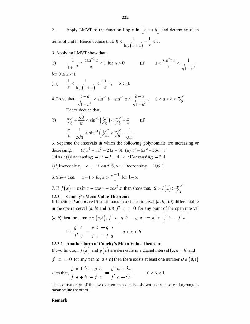
232

2. Apply LMVT to the function Log x in a a h, and determine in

terms of and h. Hence deduce that: xx

1 10 1

log 1

.

3. Applying LMVT show that:

(i) x

xx

1

2

1 tan1

1

for 0x (ii) x

x x

1

2

sin 11

1

for x0 1

(iii)

x

x xx

1 1 1,

log 1

.0x

4. Prove that, b a b a

b aa b

1 1

2 2sin sin ,

1 1

a b02

Hence deduce that,

(i) b b13 13sin

515 8 (ii)

bb11 11sin

42 3 15

5. Separate the intervals in which the following polynomials are increasing or

decreasing. (i)x x x3 23 24 31 (ii) x 3 – 6x

2 – 36x + 7

[ : ( )Increasing , 2 , 4, ;Decreasing 2,4Ans i

( )Increasing , 2 6, ;Decreasing 2,6ii and ]

6. Show that, x

x xx

11 log

for .1 x

7. If f x x x x x2sin cos cos then show that, f x22

12.2 Cauchy’s Mean Value Theorem: If functions f and g are (i) continuous in a closed interval [a, b], (ii) differentiable

in the open interval (a, b) and (iii) 0f x for any point of the open interval

(a, b) then for some c a b, , f c g b g a g c f b f a

i.e. g c g b g a

f c f b f a a c b.

12.2.1 Another form of Cauchy’s Mean Value Theorem:

If two function f x and g x are derivable in a closed interval [a, a + h] and

0f x for any x in (a, a + h) then there exists at least one number 0,1

such that, ,g a h g a g a h

f a h f a f a h 0 1

The equivalence of the two statements can be shown as in case of Lagrange‟s

mean value theorem.

Remark:

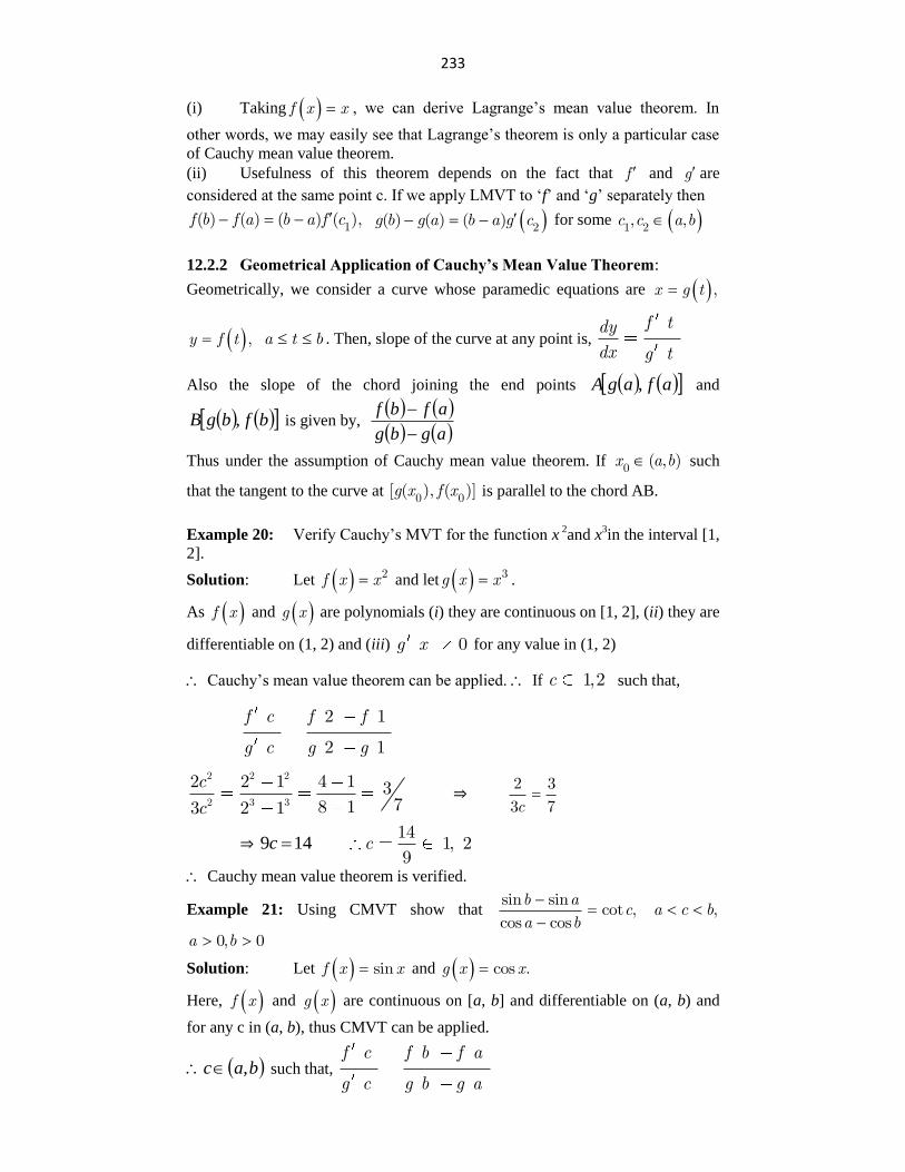
233

(i) Taking f x x , we can derive Lagrange‟s mean value theorem. In

other words, we may easily see that Lagrange‟s theorem is only a particular case

of Cauchy mean value theorem.

(ii) Usefulness of this theorem depends on the fact that f and g are

considered at the same point c. If we apply LMVT to „f‟ and „g‟ separately then

f b f a b a f c1( ) ( ) ( ) ( ), g b g a b a g c2( ) ( ) ( ) for some c c a b1 2, ,

12.2.2 Geometrical Application of Cauchy’s Mean Value Theorem:

Geometrically, we consider a curve whose paramedic equations are x g t ,

y f t , a t b . Then, slope of the curve at any point is, f tdy

dx g t

Also the slope of the chord joining the end points afagA , and

bfbgB , is given by, agbg

afbf

Thus under the assumption of Cauchy mean value theorem. If x a b0 ( , ) such

that the tangent to the curve at g x f x0 0[ ( ), ( )] is parallel to the chord AB.

Example 20: Verify Cauchy‟s MVT for the function x 2and x

3in the interval [1,

2].

Solution: Let f x x2 and let g x x 3 .

As f x and g x are polynomials (i) they are continuous on [1, 2], (ii) they are

differentiable on (1, 2) and (iii) 0g x for any value in (1, 2)

Cauchy‟s mean value theorem can be applied. If 1,2c such that,

2 1

2 1

f c f f

g c g g

2 2 2

2 3 3

2 2 1 4 1 378 13 2 1

c

c ⇒

c

2 3

3 7

⇒ 149 c c14

1, 29

Cauchy mean value theorem is verified.

Example 21: Using CMVT show that b a

ca b

sin sincot ,

cos cos

a c b,

a b0, 0

Solution: Let f x xsin and g x xcos .

Here, f x and g x are continuous on [a, b] and differentiable on (a, b) and

for any c in (a, b), thus CMVT can be applied.

bac , such that, f c f b f a

g c g b g a

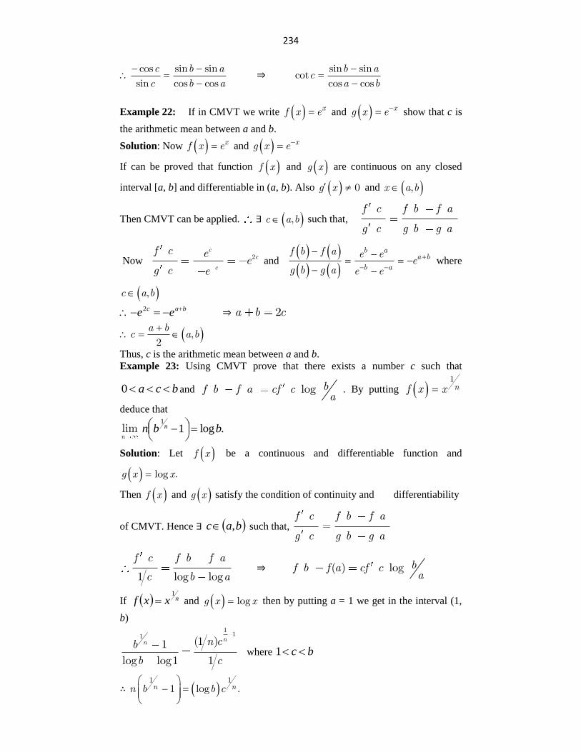
234

c b a

c b a

cos sin sin

sin cos cos

⇒

b ac

a b

sin sincot

cos cos

Example 22: If in CMVT we write xf x e and xg x e show that c is

the arithmetic mean between a and b.

Solution: Now xf x e and xg x e

If can be proved that function f x and g x are continuous on any closed

interval [a, b] and differentiable in (a, b). Also g x 0 and x a b,

Then CMVT can be applied. ∃ c a b, such that, f c f b f a

g c g b g a

Now 2

cc

c

f c ee

g c e and

b aa b

b a

f b f a e ee

g b g a e e

where

c a b,

bac ee 2 ⇒ 2a b c

a b

c a b,2

Thus, c is the arithmetic mean between a and b.

Example 23: Using CMVT prove that there exists a number c such that

bca 0 and log bf b f a cf ca

. By putting nf x x1

deduce that

limn

.log11

bbn n

Solution: Let f x be a continuous and differentiable function and

g x xlog .

Then f x and g x satisfy the condition of continuity and differentiability

of CMVT. Hence ∃ bac , such that, f c f b f a

g c g b g a

1 log log

f c f b f a

c b a ⇒ ( ) log bf b f a cf c

a

If nxxf1

and g x xlog then by putting a = 1 we get in the interval (1,

b) 1

11(1 )1

log log1 1

nn n cb

b c where bc 1

∴ n nn b b c1 1

1 log .

235

limn

nn b b1

1 log

[ nc1

1 as n ]

Example 24: If ba 1 , show that there exists c satisfying bca such

that

b ab

a c

2 2

2log

2

Solution: We have to prove that, b a

b a c2 2 2

log log 1

2

This suggests us to take f x xlog and g x x2 Now, f x and g x are

continuous on [a, b] and differentiable on (a, b) and 0g x for any c in (a,

b).

CMVT can be applied. ∃ c a b, such that,

f c f b f a

g c g b g a ⇒

b acc b a2 2

1log log

2

∴ b a

c b a2 2 2

1 log log

2

⇒

b aba c

2 2

2log

2

Check Your Progress

1. Find c of Cauchy‟s mean value theorem for:

(i) xxf , ,1

xxg ],,[ bax 0a (ii) sin ,f x x

cosg x x on ]2

,0[

(iii) ,23 xxf 12 xxg on .41 x (iv) ,xexf

xexg on [0, 1]

(v) ,xexf ,12

2

x

xxg ]1,1[x

[Ans :- (i) ab (ii) 4 (iii) 25 (iv) 21 (v) 0.]

12.3 Summary

In this chapter we have learnt about the mean value theorems. The

Rolle‟s theorem which is the fundamental theorem in analysis has been proved.

The Lagrange‟s MVT and the Cauchy‟s MVT have also been proved. Problems

based on these theorems have been done in order to understand the Mean Value

theorems. In the next chapter we are going to learn about Taylor‟s theorem and

its applications.

12.4 Unit End Exercise:

1. Verify Rolle‟s theorem for each of the following:

) ( ) ( 1)( 2)( 3) in [-1,1]i f x x x x

2) ( ) ( 3) in [0,3]ii f x x x

) ( ) tan 2 in [0, ]iii f x x

2) ( ) 4 in [-2, 2]iv f x x

236 2. Verify LMVT for the following functions.

2) ( ) 1 in [-1, 1]i f x x

) ( ) ( 1)( 4)( 3) in [0, 7]ii f x x x x

2) ( ) ( 1) in [0, 2]iii f x x x

3. Find „c‟ of CMVT for the following: 2 3) ( ) , ( ) in [1,2]i f x x g x x

2) ( ) 2 4, ( ) 3 in [0,2]ii f x x x g x x

2) ( ) ( 1) 4, ( ) 1 in [0,2]iii f x x g x x

***********

237

APPROXIMATION, ERRORS AND EXTREMA 13

Unit Structure

13.1 Introduction

13.2 Objectives

13.3 Approximation

13.4 Maxima and Minima

13.5 Let Us Sum Up

13.1 INTRODUCTION In the previous units we have seen how we can successively differentiate a

function, partial differentiation of a function and also various mean value

theorems. Differential Calculus has various applications. Some of the physical

and geometrical applications we have seen before. Derivatives can also be used

to find maximum and minimum values of a function in an interval. The

maximum and minimum values are called extreme values of a function. The

extreme values can be absolute or can be local. The first derivative test and the

second derivative tests are used to determine the points of local extrema. In this

chapter we are going to use the differential calculus concept to answer questions

like:

(1) What is the approximate value of sin1 ?

(2) What is the error in calculating the area of a square, if the error in

calculating the side length was 1%?

(3) What are the maximum and minimum values of a function in a given

interval?

13.2 OBJECTIVES

After studying this unit you should be able to:

compute the approximate value of a function at a given point.

compute error, relative error and percentage error

compute maxima and minima for a function in a given interval.

13.3 ERRORS and APPROXIMATION

Let ( , )z f x y be a differentiable function. Let x denote the error in x

and y denote the error in y. Then the corresponding error in z denoted by z is

given by:

z zz x y

x y

The above formula can be extended to more than two variables also. For

example, if u = f(x, y, z) then continuing with the same notations,

u u uu x y z

x y z

.

Relative error: If z is an error in z then the relative error in z is given by: z

z

.

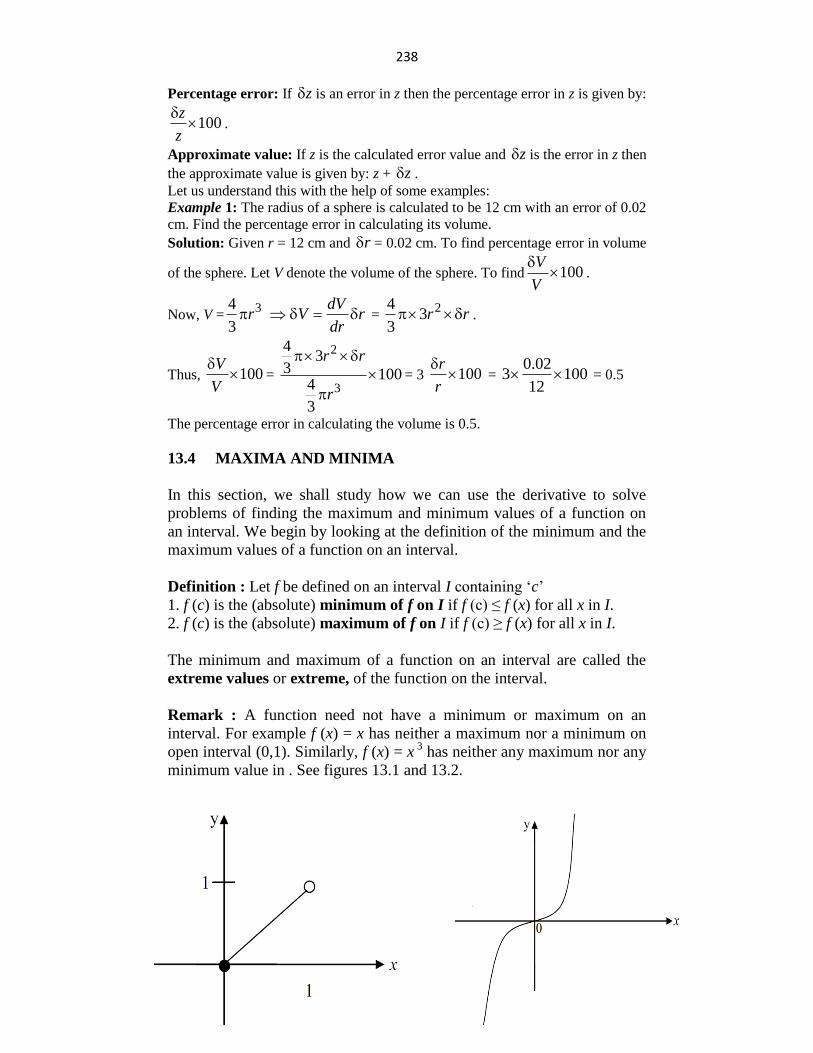
238

Percentage error: If z is an error in z then the percentage error in z is given by:

100z

z

.

Approximate value: If z is the calculated error value and z is the error in z then

the approximate value is given by: z + z .

Let us understand this with the help of some examples:

Example 1: The radius of a sphere is calculated to be 12 cm with an error of 0.02

cm. Find the percentage error in calculating its volume.

Solution: Given r = 12 cm and r = 0.02 cm. To find percentage error in volume

of the sphere. Let V denote the volume of the sphere. To find 100V

V

.

Now, V =34

3r

dVV r

dr =

234

3r r .

Thus, 100V

V

=

2

3

4

3 14

3

00

3

rr

r

= 3 100r

r

=

0.023 100

12 = 0.5

The percentage error in calculating the volume is 0.5.

13.4 MAXIMA AND MINIMA

In this section, we shall study how we can use the derivative to solve

problems of finding the maximum and minimum values of a function on

an interval. We begin by looking at the definition of the minimum and the

maximum values of a function on an interval.

Definition : Let f be defined on an interval I containing „c‟

1. f (c) is the (absolute) minimum of f on I if f (c) ≤ f (x) for all x in I.

2. f (c) is the (absolute) maximum of f on I if f (c) ≥ f (x) for all x in I.

The minimum and maximum of a function on an interval are called the

extreme values or extreme, of the function on the interval.

Remark : A function need not have a minimum or maximum on an

interval. For example f (x) = x has neither a maximum nor a minimum on

open interval (0,1). Similarly, f (x) = x 3

has neither any maximum nor any

minimum value in . See figures 13.1 and 13.2.

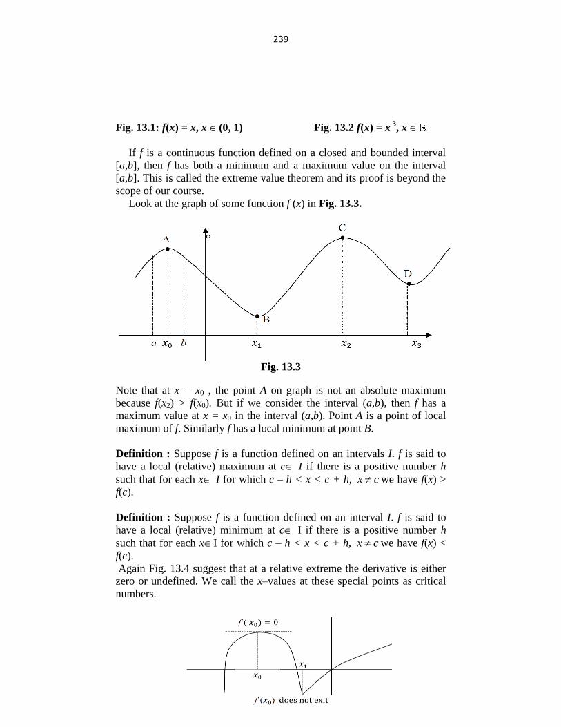
239

Fig. 13.1: f(x) = x, x (0, 1) Fig. 13.2 f(x) = x 3

, x

If f is a continuous function defined on a closed and bounded interval

[a,b], then f has both a minimum and a maximum value on the interval

[a,b]. This is called the extreme value theorem and its proof is beyond the

scope of our course.

Look at the graph of some function f (x) in Fig. 13.3.

Fig. 13.3

Note that at x = x0 , the point A on graph is not an absolute maximum

because f(x2) > f(x0). But if we consider the interval (a,b), then f has a

maximum value at x = x0 in the interval (a,b). Point A is a point of local

maximum of f. Similarly f has a local minimum at point B.

Definition : Suppose f is a function defined on an intervals I. f is said to

have a local (relative) maximum at c I if there is a positive number h

such that for each x I for which c – h < x < c + h, x c we have f(x) >

f(c).

Definition : Suppose f is a function defined on an interval I. f is said to

have a local (relative) minimum at c I if there is a positive number h

such that for each xI for which c – h < x < c + h, x c we have f(x) <

f(c).

Again Fig. 13.4 suggest that at a relative extreme the derivative is either

zero or undefined. We call the x–values at these special points as critical

numbers.

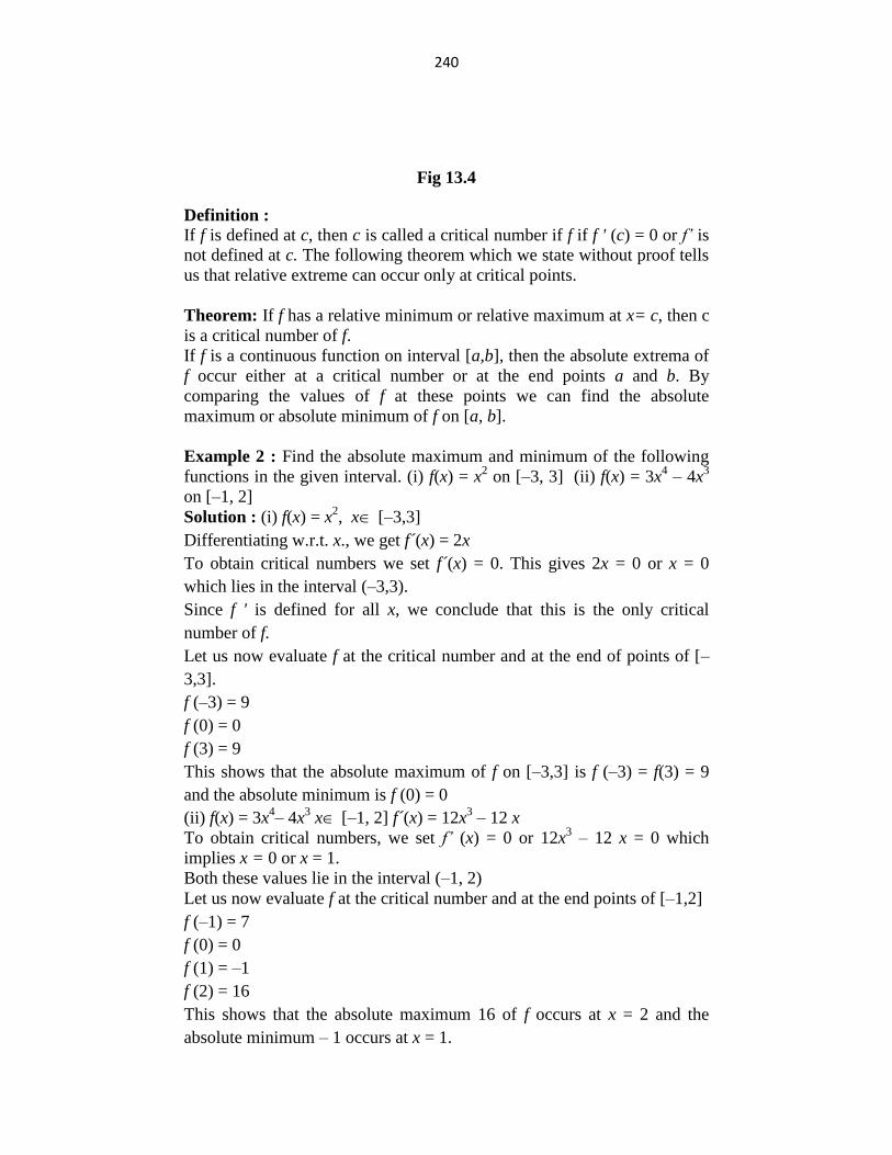
240

Fig 13.4

Definition :

If f is defined at c, then c is called a critical number if f if f ' (c) = 0 or f’ is

not defined at c. The following theorem which we state without proof tells

us that relative extreme can occur only at critical points.

Theorem: If f has a relative minimum or relative maximum at x= c, then c

is a critical number of f.

If f is a continuous function on interval [a,b], then the absolute extrema of

f occur either at a critical number or at the end points a and b. By

comparing the values of f at these points we can find the absolute

maximum or absolute minimum of f on [a, b].

Example 2 : Find the absolute maximum and minimum of the following

functions in the given interval. (i) f(x) = x2 on [–3, 3] (ii) f(x) = 3x

4 – 4x

3

on [–1, 2]

Solution : (i) f(x) = x2, x [–3,3]

Differentiating w.r.t. x., we get f´(x) = 2x

To obtain critical numbers we set f´(x) = 0. This gives 2x = 0 or x = 0

which lies in the interval (–3,3).

Since f ' is defined for all x, we conclude that this is the only critical

number of f.

Let us now evaluate f at the critical number and at the end of points of [–

3,3].

f (–3) = 9

f (0) = 0

f (3) = 9

This shows that the absolute maximum of f on [–3,3] is f (–3) = f(3) = 9

and the absolute minimum is f (0) = 0

(ii) f(x) = 3x4– 4x

3 x [–1, 2] f´(x) = 12x

3 – 12 x

To obtain critical numbers, we set f’ (x) = 0 or 12x3 – 12 x = 0 which

implies x = 0 or x = 1.

Both these values lie in the interval (–1, 2)

Let us now evaluate f at the critical number and at the end points of [–1,2]

f (–1) = 7

f (0) = 0

f (1) = –1

f (2) = 16

This shows that the absolute maximum 16 of f occurs at x = 2 and the

absolute minimum – 1 occurs at x = 1.

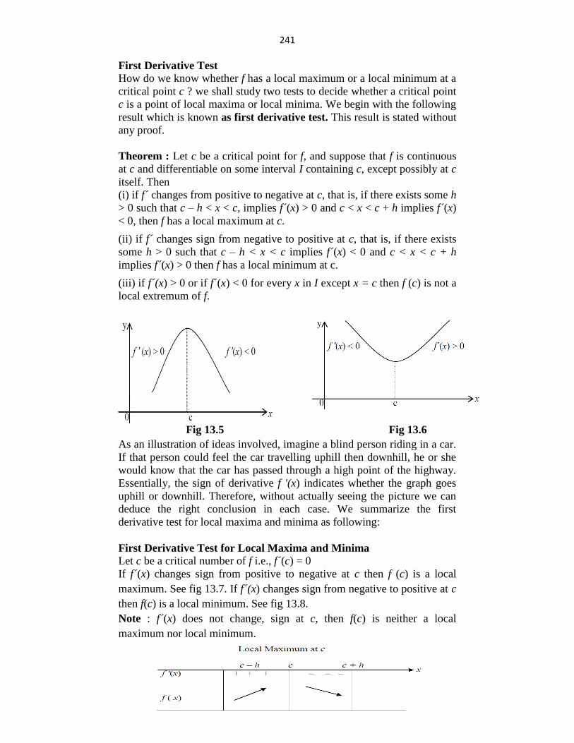
241

First Derivative Test How do we know whether f has a local maximum or a local minimum at a

critical point c ? we shall study two tests to decide whether a critical point

c is a point of local maxima or local minima. We begin with the following

result which is known as first derivative test. This result is stated without

any proof.

Theorem : Let c be a critical point for f, and suppose that f is continuous

at c and differentiable on some interval I containing c, except possibly at c

itself. Then

(i) if f´ changes from positive to negative at c, that is, if there exists some h

> 0 such that c – h < x < c, implies f´(x) > 0 and c < x < c + h implies f´(x)

< 0, then f has a local maximum at c.

(ii) if f´ changes sign from negative to positive at c, that is, if there exists

some h > 0 such that c – h < x < c implies f´(x) < 0 and c < x < c + h

implies f´(x) > 0 then f has a local minimum at c.

(iii) if f´(x) > 0 or if f´(x) < 0 for every x in I except x = c then f (c) is not a

local extremum of f.

Fig 13.5 Fig 13.6

As an illustration of ideas involved, imagine a blind person riding in a car.

If that person could feel the car travelling uphill then downhill, he or she

would know that the car has passed through a high point of the highway.

Essentially, the sign of derivative f '(x) indicates whether the graph goes

uphill or downhill. Therefore, without actually seeing the picture we can

deduce the right conclusion in each case. We summarize the first

derivative test for local maxima and minima as following:

First Derivative Test for Local Maxima and Minima Let c be a critical number of f i.e., f´(c) = 0

If f´(x) changes sign from positive to negative at c then f (c) is a local

maximum. See fig 13.7. If f´(x) changes sign from negative to positive at c

then f(c) is a local minimum. See fig 13.8.

Note : f´(x) does not change, sign at c, then f(c) is neither a local

maximum nor local minimum.

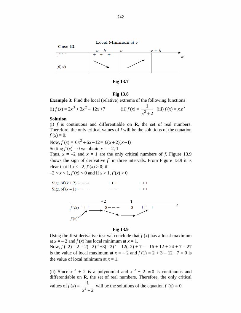
242

Fig 13.7

Fig 13.8

Example 3: Find the local (relative) extrema of the following functions :

(i) f (x) = 2x 3

+ 3x 2

– 12x +7 (ii) f (x) = 2

1

2x (iii) f (x) = x.e

x

Solution (i) f is continuous and differentiable on R, the set of real numbers.

Therefore, the only critical values of f will be the solutions of the equation

f´(x) = 0.

Now, f´(x) = 26 6 12x x = 6( 2)( 1)x x

Setting f´(x) = 0 we obtain x = – 2, 1

Thus, x = –2 and x = 1 are the only critical numbers of f. Figure 13.9

shows the sign of derivative f´ in three intervals. From Figure 13.9 it is

clear that if x < –2, f´(x) > 0; if

–2 < x < 1, f´(x) < 0 and if x > 1, f´(x) > 0.

Fig 13.9

Using the first derivative test we conclude that f (x) has a local maximum

at x = – 2 and f (x) has local minimum at x = 1.

Now, f (–2) – 2 = 2(– 2) 3

+3(– 2) 2

– 12(–2) + 7 = –16 + 12 + 24 + 7 = 27

is the value of local maximum at x = – 2 and f (1) = 2 + 3 – 12+ 7 = 0 is

the value of local minimum at x = 1.

(ii) Since x 2

+ 2 is a polynomial and x 2

+ 2 0 is continuous and

differentiable on R, the set of real numbers. Therefore, the only critical

values of f (x) = 2

1

2x will be the solutions of the equation f '(x) = 0.

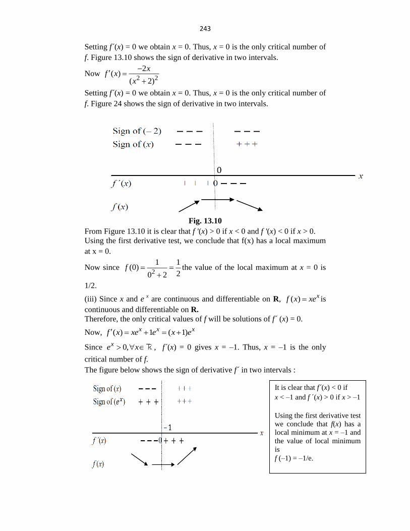
243

Setting f´(x) = 0 we obtain x = 0. Thus, x = 0 is the only critical number of

f. Figure 13.10 shows the sign of derivative in two intervals.

Now 2 2

(( )

)2

2xf x

x

Setting f´(x) = 0 we obtain x = 0. Thus, x = 0 is the only critical number of

f. Figure 24 shows the sign of derivative in two intervals.

Fig. 13.10

From Figure 13.10 it is clear that f '(x) > 0 if x < 0 and f '(x) < 0 if x > 0.

Using the first derivative test, we conclude that f(x) has a local maximum

at x = 0.

Now since 2

1 1(0)

20 2f

the value of the local maximum at x = 0 is

1/2.

(iii) Since x and e x

are continuous and differentiable on R, ( ) xf x xe is

continuous and differentiable on R.

Therefore, the only critical values of f will be solutions of f´ (x) = 0.

Now, ( ) 1 ( 1)x x xf x xe e x e

Since 0,x xe , f´(x) = 0 gives x = –1. Thus, x = –1 is the only

critical number of f.

The figure below shows the sign of derivative f´ in two intervals :

It is clear that f´(x) < 0 if

x < –1 and f ´(x) > 0 if x > –1

Using the first derivative test

we conclude that f(x) has a

local minimum at x = –1 and

the value of local minimum

is

f (–1) = –1/e.

244

Second Derivative Test

The first derivative test is very useful for finding the local maxima and

local minima of a function. But it is slightly cumbersome to apply as we

have to determine the sign of f ' around the point under consideration.

However, we can avoid determining the sign of derivative f ' around the

point under consideration, say c, if we know the sign of second derivative

f at point c. We shall call it as the second derivative test.

Theorem : (Second Derivative Test)

Let f(x) be a differentiable function on I and let c I. Let f ´ (x) be

continuous at c. Then

1. c is a point of local maximum if both f '(c) = 0 and f (c) < 0.

2. c is a point of local minimum if both f '(c) = 0 and f (c) > 0.

Remark : If f´(c) = 0 and f´´(c) = 0, then the second derivative test fails. In

this case, we use the first derivative test to determine whether c is a point

of local maximum or a point of a local minimum.

We summarize the second – derivative test for local maxima and minima

in the following table.

Second Derivative Test for Local Maxima and Minima

( )f c ( )f c ( )f c

0 + Local Minimum

0 - Local Maximum

0 0 Test Fails

We shall adopt the following step to determine local maxima and minima.

Steps to find Local Maxima and Local Minima

The function f is assumed to posses the second derivative on the interval I.

Step 1 : Find f ' (x) and set it equal to 0.

Step 2 : Solve f ' (x) = 0 to obtain the critical numbers of f. Let the

solution of this equation be α, ………. We shall consider only those

values of x which lie in I and which are not end points of I.

Step 3 : Evaluate f ´ (α) If f (α) < 0, f (x) has a local maximum at x = α and

its value if f (α) If f (α) > 0, f (x) has a local minimum at x = α and its value

if f (α) If f (α) = 0, apply the first derivative test.

Step 4 : If the list of values in Step 2 is not exhausted, repeat step 3, with

that value.

Example 4: Find the points of local maxima and minima, if any, of each

of the following functions. Find also the local maximum values and local

minimum values.

(i) f (x) = 3 26 9 1xx x , x

245

(ii) f(x) = 3 2 22 ( 0),x ax a x a x

Solution:

(i) f ´ (x) = 23 12 9x x = 3( 1)( 3)x x

To obtain critical number of f, we set f ´ (x) = 0 this yields x = 1, 3.

Therefore, the critical number of f are x = 1, 3.

Now f ´ (x) = 6x – 12 = 6(x – 2)

We have f ´ (1) = 6(1 – 2) = – 6 < 0 and f (3) = 6(3 – 2) = 6 > 0.

Using the second derivative test, we see that f (x) has a local maximum at

x = 1 and a local minimum at x = 3. The value of local maximum at x = 1 is f

(1) = 1– 6+ 9 +1 = 5 and the value of local minimum at x = 3 is

f (3) = 33 – 6(3)2 + 9(3) + 1 = 27 – 54 + 27 + 1 = 1.

(ii) We have f(x) = 3 2 22 ( 0)x ax a x a

Thus, 2 2( ) 3 4 (3 )( )ax a x af x x x a

As f '(x) is defined for each x R, to obtain critical number of f we set

f '(x) = 0.

This yields x = a/3 or x = a.

Therefore, the critical numbers of f and a/3 and a. Now, ( )f a = 6x – 4a.

We have ( / 3) 6( / 3) 4 2 0f a a a a

and ( ) 6 4 2 0f a a a a

Using the second derivative test, we see that f(x) has a local maximum at x

= a/3 and a local minimum at x = a.

The value of local maximum at / 3x a is 34

( / 3)27

f a a and the value

of local minimum at x = a is ( ) 0f a .

Check Your Progress 1. Find the absolute maximum and minimum of the following functions in

the given intervals.

(i) f(x) = 4 – 7 x + 3 on [–2, 3]

(ii) f(x) =3

2

x

x on [–1,1]

2. Using first derivative test find the local maxima and minima of the

following functions.

(i) 3( ) 12f x x x (ii) 2

( ) , 02

xf x x

x

3. Use second derivative test to find the local maxima and minima of the

following functions.

(i) 3 2( ) 2 1,f x x x x x (ii) ( ) 2 1 , 1f x x x x

246

13.5 LET US SUM UP

The chapter is, as suggested by the title, on applications of differential

calculus. In section 13.4, methods for finding out (local) maxima and

minima, are discussed and explained with examples.

Documents

MATRICES - Muarchive.mu.ac.in/myweb_test/syllFybscit/APM.pdf · 1 1 MATRICES UNIT STRUCTURE 1.0 Objectives 1.1 Introduction 1.2 Definitions 1.3 Illustrative examples 1.4 Rank of matrix