Embed Size (px)
Citation preview
FOXES TEAM Reference Guide for Matrix.xla
Matrices and
Linear Algebra
Volume
R E F E R E NC E G U I D E F O R M AT R I X . X L A
Matrices and Linear Algebra
T U T O R I A L F O R M A T R I X . X L A
2
Index About Matrix.xla ........................................................................................................................ 6
Matrix.xla ................................................................................................................................. 6
Array functions ......................................................................................................................... 7 What is an array function ........................................................................................................ 7 How to insert an array function ............................................................................................... 7
How to get help on line .......................................................................................................... 11
MATRIX installation ................................................................................................................ 12 How to install ......................................................................................................................... 12 Update to a new version ....................................................................................................... 13 How to uninstall ..................................................................................................................... 13
About complex matrix formats.............................................................................................. 14
Functions Reference .............................................................................................................. 16 Function MAbs(V).................................................................................................................. 17 Function MAbsC(V, [Cformat]) .............................................................................................. 17 Function MAdd(A, B)............................................................................................................. 17 Function MAddC(A, B, [Cformat]) ......................................................................................... 18 Function MBAB(A, B) ............................................................................................................ 18 Function MDet(Mat, Mat, [IMode], [Tiny]).............................................................................. 18 Function MDetC (Mat, [Cformat]) .......................................................................................... 19 Function MDet3(Mat3) .......................................................................................................... 20 Function MDetPar(Mat) ......................................................................................................... 20 Function MInv(Mat, [IMode], [Tiny]) ...................................................................................... 21 Function MPseudoInv (A)...................................................................................................... 21 Function MPow(A, n)............................................................................................................. 22 Function MPowC(A, n, [Cformat]) ......................................................................................... 22 Function MExp(A, [Algo], [n]) ................................................................................................ 22 Function MExpErr(A, n)......................................................................................................... 22 Function MProd(A, B, ...)....................................................................................................... 23 Function MMultS(Mat, k) ....................................................................................................... 23 Function MMultSC(Mat, scalar, [Cformat])............................................................................ 24 Function MMult3(Mat3, Mat) ................................................................................................. 24
T U T O R I A L F O R M A T R I X . X L A
3
Function MMultTpz(tpz, v)..................................................................................................... 25 Function MSub(A1, A2) ......................................................................................................... 25 Function MSubC(A1, A2, [Cformat]) ..................................................................................... 26 Function MTrace(Mat) ........................................................................................................... 26 Function MDiag(Diag) ........................................................................................................... 26 Function MDiagExtr(Mat, [Diag])........................................................................................... 26 Function MT(Mat) .................................................................................................................. 27 Function MTC(Mat, [Cformat]) .............................................................................................. 27 Function MTH(Mat, [Cformat]) .............................................................................................. 27 Function MRank(A) ............................................................................................................... 28 Function MIde(n) ................................................................................................................... 28 Function ProdScal(v1, v2)..................................................................................................... 28 Function ProdVect(v1, v2)..................................................................................................... 29 Function VectAngle(v1, v2) ................................................................................................... 29 Function MEigenvalJacobi(Mat, Optional MaxLoops)........................................................... 30
Eigenvalues problem with Jacobi, step by step ................................................................................31 Function MRotJacobi(Mat) .................................................................................................... 32 Function MBlock(Mat) ........................................................................................................... 32 Function MBlockPerm(Mat)................................................................................................... 33 Function MEigenvalQR(Mat)................................................................................................. 34 Function MEigenvalQRC(Mat, [Cformat]) ............................................................................. 35 Function MEigenvec(A, Eigenvalues, [MaxErr]) ................................................................... 35 Function MEigenvecC(A, Eigenvalue, [MaxErr])................................................................... 36 Function MEigenvecJacobi(Mat, Optional MaxLoops).......................................................... 37 Function MEigenSortJacobi(EigvalM, EigvectM, [num]) ....................................................... 37 Function MEigenvalQL(Mat3, [IterMax]) ............................................................................... 37 Function MEigenvalTTpz(n, a, b, c) ...................................................................................... 38 Function MEigenvecT(Mat3, Eigenvalues, [MaxErr])........................................................... 39 Function MChar(A, x) ............................................................................................................ 40 Function MCharC( A, z, [Cformat])........................................................................................ 40 Function MCharPoly(Mat) ..................................................................................................... 41 Function MCharPolyC( Mat, [CFormat])................................................................................ 41 Function PolyRoots(poly) ...................................................................................................... 42 Function MEigenvalMax(Mat, [IterMax]) ............................................................................... 42
A global localization method for real eigenvalues .............................................................................42 Function MEigenvecMax(Mat, [Norm], [IterMax]) ................................................................. 43 Function MEigenvalPow(Mat, [IterMax]) ............................................................................... 44 Function MEigenvecPow(Mat, [Norm], [IterMax]) ................................................................. 44
T U T O R I A L F O R M A T R I X . X L A
4
Function MEigenvecInv(Mat, Eigenvalue) ............................................................................ 44 Function MEigenvecInvC(Mat, Eigenvalue, [CFormat])........................................................ 45
About perturbed eigenvalues............................................................................................................45 Matrix Generator ................................................................................................................... 47 Function GJstep(Mat, [Typ], [IntValue], [tiny])....................................................................... 50 Function SysLin(A, b, [IMode], [Tiny]) ................................................................................... 52 Function SysLin3(Mat3, y) .................................................................................................... 53 Function SysLinIterG(A, b, x0, [Nmax], [w]) .......................................................................... 53 Function SysLinT(Mat, b, [typ], [tiny]).................................................................................... 54 Function SysLinIterJ(A, b, x0, [Nmax]).................................................................................. 55 Function SysLinSing(A, [b], [MaxErr]) ................................................................................... 55 Function SysLinTpz(A, b) ...................................................................................................... 57 Function TraLin(A, x, [B]) ...................................................................................................... 58
Matrix Geometric action....................................................................................................................58 Function MOrthoGS(A) ......................................................................................................... 59
Gram-Schmidt Orthogonalization......................................................................................................60 Function MCholesky(A) ......................................................................................................... 61 Function MLU(A, optional Pivot) ........................................................................................... 61 Function MQR(Mat)............................................................................................................... 63 Function MQRiter(Mat, [MaxLoops]) ..................................................................................... 64 Function MQH(A, b) .............................................................................................................. 65 Function MExtract(A, i_pivot, j_pivot).................................................................................... 65 Function PathFloyd(G) .......................................................................................................... 66 Function PathMin(G) ............................................................................................................. 66
Graphs theory recalls........................................................................................................................66 Shortest path ....................................................................................................................................69
Singular Value Decomposition -........................................................................................... 71 Condition Number ................................................................................................................. 72 Function MMopUp(M, [ErrMin])............................................................................................. 74 Function MCovar(A) .............................................................................................................. 74 Function MCorr(A)................................................................................................................. 74 Function RegrL(Y, X, [Intcpt] )............................................................................................... 75 Function RegrP(Degree, Y, X, [Intcpt] ) ................................................................................ 77 Function RegrCir( X, Y ) ........................................................................................................ 78 Function MCmp(Coeff) .......................................................................................................... 79 Function MCplx([Ar], [Ai], [Cformat]) ..................................................................................... 79 Function PolyRootsQR(poly)................................................................................................. 80 Function PolyRootsQRC(Coefficients).................................................................................. 80 Function MRot(n, theta, p, q) ................................................................................................ 81 Function VarimaxRot(FL, [Normal], [MaxErr], [MaxIter])....................................................... 82
T U T O R I A L F O R M A T R I X . X L A
5
Function VarimaxIndex(Mat, [Normal]) ................................................................................. 83 Function MNormalize(Mat, [NormType], [Tiny]) .................................................................... 83 Function MNormalizeC(Mat, [NormType], [Cformat], [Tiny])................................................. 83 Function MNorm(v, [NORM]) ................................................................................................ 84 Function MMultC(M1, M2, [Cformat]).................................................................................... 85 Function MInvC(A, [Cformat]) ............................................................................................... 86 Function ProdScalC(v1, v2, ) ................................................................................................ 86 Function SysLinC(A, b, [Cformat]) ........................................................................................ 87 Function Simplex(Funct, Constraint, [Opt])........................................................................... 88 Function MPerm(Permutations) ............................................................................................ 90 Function MHessenberg(Mat)................................................................................................. 90 Function MAdm(Branch) ....................................................................................................... 91
Linear Electric Network.....................................................................................................................91 Thermal Network ..............................................................................................................................92
Function MLeontInv(ExTab, Tot)........................................................................................... 94 Input Output Analysis........................................................................................................................94
Matrix Tool............................................................................................................................... 95 The Matrix toolbar ................................................................................................................. 95
Selector tool......................................................................................................................................95 Matrix Generator...............................................................................................................................98
Macro stuff........................................................................................................................... 102 Matrix operations ............................................................................................................................102 Sparse Matrix operations................................................................................................................103 Complex Matrix operations .............................................................................................................104 Macro Gauss-step-by-step .............................................................................................................105 Macro Shortest-Path.......................................................................................................................106 Macro Draw Graph .........................................................................................................................106 Macro Block reduction ....................................................................................................................107
References............................................................................................................................. 108
Credits.................................................................................................................................... 109
D E S I G N C U S T O M I Z A T I O N
About Matrix.xla About Matrix.xla Matrix.xla Matrix.xla is an Excel add-in that contains useful functions for matrices and linear Algebra:
Norm. Matrix multiplication. Similarity transformation. Determinant. Inverse. Power. Trace. Scalar Product. Vector Product.
Eigenvalues and Eigenvectors of a symmetric matrix with Jacobi algorithm. Jacobi's rotation matrix. Eigenvalues with the QR and QL algorithm. Characteristic polynomials. Polynomial roots with the QR algorithm. Eigenvectors for real and complex matrices
Generation of a random matrix with given eigenvalues or of given Rank or Determinant. Generation of useful matrices: Hilbert's, Householder's, Tartaglia's. Vandermonde's
Solving a system of linear equations: Linear System with iterative methods: Gauss-Seidel and Jacobi algorithms. Gauss-Jordan algorithm, step by step. Singular Linear System.
Linear Transformations:. Gram-Schmidt Orthogonalization. Matrix factorizations: LU, QR, SVD and Cholesky decomposition.
This tutorial is divided into two parts. The first part is the reference manual of Matrix.xla. The second part explains with practical examples how to solve several basic problems in matrix theory and linear algebra. Why Matrix.xla has the same functions as Excel? Yes, The same functions, such as determinant, inversion, multiplication, and transpose, are in both Excel and Matrix.xla. They perform the same tasks. And in many case they return the same values. But they are not exchangeable in every situation.
The main difference lies in the algorithms used; in other words, in the way in which the functions are implemented. In Matrix.xla, the algorithms are open, and people can verify how each function works. The function that performs matrix inversion in Excel and in Matrix.xla, for example, can give different results, especially in high-accuracy calculations. Their main difference is that the
Matrix.xla Inversion function uses the popular Gauss-Jordan algorithm - explained in many books and web pages - while the Excel built-in functions are written in inaccessible, proprietary code. In a few other cases we have simply created new functions to avoid the original, verbose names (MTRANSPOSE(), or MATR.TRASPOSTA () in Italian version, are substituted by the more handy MT() )
Chapter
1
Matrix.xla algorithms are open
T U T O R I A L F O R M A T R I X . X L A
7
Array functions What is an array function A function that returns multiple values is called an "array function". Matrix.xla contains lots of these functions. All functions that return a matrix are array functions. Inversion, multiplication, sum, vector product, etc. are examples of array functions. On the contrary, Norm and Scalar product are scalar functions because they return only one value.
In a worksheet, an array function returns always a rectangular (n x m) range of cells. To insert this function, select before the (n x m ) range where you want to insert the function, then, you must use the keys sequence CTRL+SHIFT+ENTER;. The sequence must be used just after inserting the function parameters. Keep down both CTRL and SHIFT keys (the order of depressing them doesn't matter) and then press ENTER.
If you miss this sequence or use only the ENTER key, the function only returns the first cell of the array
How to insert an array function The following example explains, step-by-step, how it works
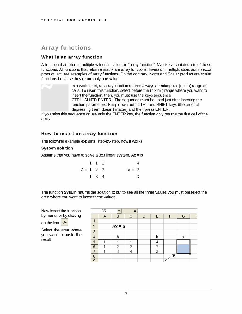
System solution Assume that you have to solve a 3x3 linear system. Ax = b
=
431221111
A
=
324
b
The function SysLin returns the solution x; but to see all the three values you must preselect the area where you want to insert these values.
Now insert the function by menu, or by clicking
on the icon
Select the area where you want to paste the result
Ä
T U T O R I A L F O R M A T R I X . X L A
8
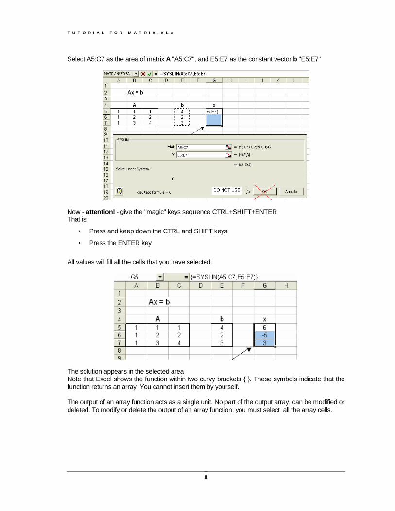
Select A5:C7 as the area of matrix A "A5:C7", and E5:E7 as the constant vector b "E5:E7"
Now - attention! - give the "magic" keys sequence CTRL+SHIFT+ENTER That is:
• Press and keep down the CTRL and SHIFT keys
• Press the ENTER key
All values will fill all the cells that you have selected.
The solution appears in the selected area Note that Excel shows the function within two curvy brackets { }. These symbols indicate that the function returns an array. You cannot insert them by yourself. The output of an array function acts as a single unit. No part of the output array, can be modified or deleted. To modify or delete the output of an array function, you must select all the array cells.
T U T O R I A L F O R M A T R I X . X L A
9
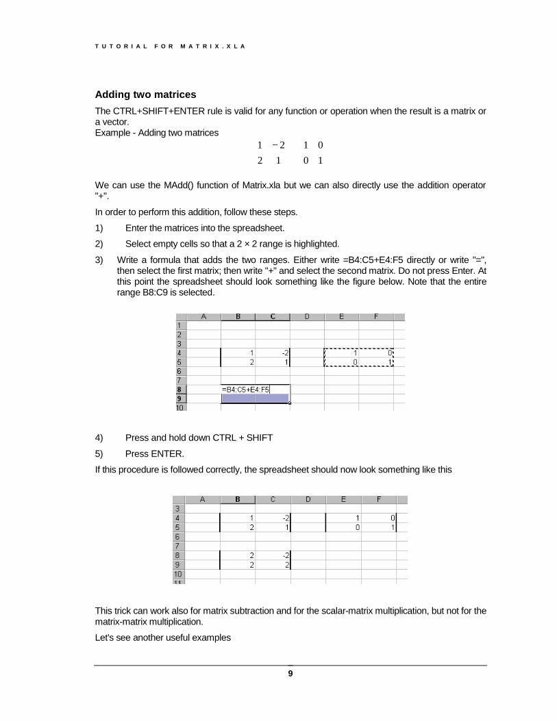
Adding two matrices The CTRL+SHIFT+ENTER rule is valid for any function or operation when the result is a matrix or a vector. Example - Adding two matrices
+
−1001
1221
We can use the MAdd() function of Matrix.xla but we can also directly use the addition operator "+".
In order to perform this addition, follow these steps.
1) Enter the matrices into the spreadsheet.
2) Select empty cells so that a 2 × 2 range is highlighted.
3) Write a formula that adds the two ranges. Either write =B4:C5+E4:F5 directly or write "=", then select the first matrix; then write "+" and select the second matrix. Do not press Enter. At this point the spreadsheet should look something like the figure below. Note that the entire range B8:C9 is selected.
4) Press and hold down CTRL + SHIFT
5) Press ENTER.
If this procedure is followed correctly, the spreadsheet should now look something like this
This trick can work also for matrix subtraction and for the scalar-matrix multiplication, but not for the matrix-matrix multiplication.
Let's see another useful examples
T U T O R I A L F O R M A T R I X . X L A
10
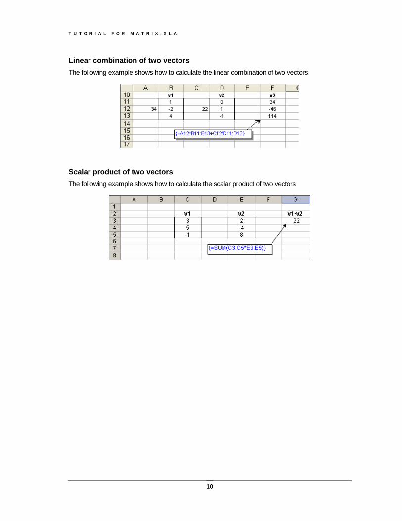
Linear combination of two vectors The following example shows how to calculate the linear combination of two vectors
Scalar product of two vectors The following example shows how to calculate the scalar product of two vectors
T U T O R I A L F O R M A T R I X . X L A
11
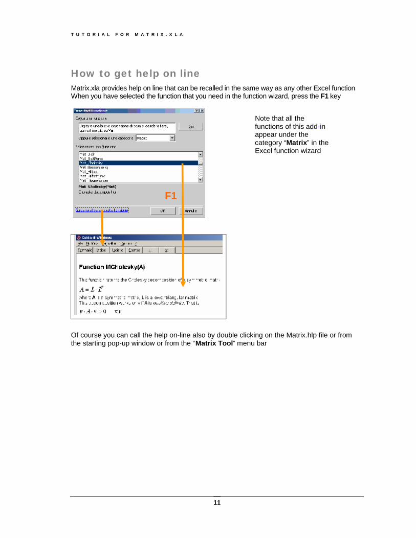
How to get help on line Matrix.xla provides help on line that can be recalled in the same way as any other Excel function When you have selected the function that you need in the function wizard, press the F1 key
Of course you can call the help on-line also by double clicking on the Matrix.hlp file or from the starting pop-up window or from the “Matrix Tool” menu bar
F1
Note that all the functions of this add-in appear under the category “Matrix” in the Excel function wizard
T U T O R I A L F O R M A T R I X . X L A
12
MATRIX installation MATRIX add-in for Excel is a zip file composed of the following files:
• MATRIX.XLA Excel add-in file • MATRIX.HLP Help file • MATRIX.CSV Function information (only for XNUMBERS add-in) • FUNCUSTOMIZE.DLL1 Dynamic Library for add-in
How to install Unzip and place all the above files in a folder of your choice. The add-in is contained entirely in this directory. Your system is not modified in any other way. If you want to uninstall this package, simply delete its folder - it's as simple as that!
To install, follow the usual procedure for installing an Excel add-in:
1) Open Excel
2) From the Excel menu toolbar select "Tools" and then select "Add-in"..
3) Once in the Add-in Manager, browse for “Matrix.xla” and select it
4) Click OK
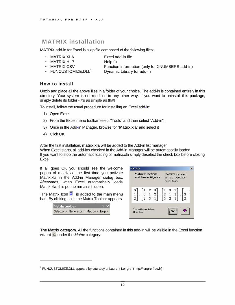
After the first installation, matrix.xla will be added to the Add-in list manager When Excel starts, all add-ins checked in the Add-in Manager will be automatically loaded If you want to stop the automatic loading of matrix.xla simply deselect the check box before closing Excel If all goes OK you should see the welcome popup of matrix.xla the first time you activate Matrix.xla in the Add-in Manager dialog box. Afterwards, when Excel automatically loads Matrix.xla, this popup remains hidden.
The Matrix Icon is added to the main menu bar. By clicking on it, the Matrix Toolbar appears
The Matrix category. All the functions contained in this add-in will be visible in the Excel function wizard under the Matrix category.
1 FUNCUSTOMIZE.DLL appears by courtesy of Laurent Longre ( http://longre.free.fr)
T U T O R I A L F O R M A T R I X . X L A
13
Update to a new version When you update to a new version you must replace the older files with the new version. Do not keep two different versions on your PC, and, in general, never load two different versions, because Excel would make a mess of it.
How to uninstall This package never alters your system files If you want to uninstall this package, simply delete its folder. Once you have canceled the Matrix.xla file, remove the corresponding entry in the Add-in Manager list, by following these steps:
1) Open Excel
2) Select <Add-in...> from the <Tools> menu.
3) Once in the Add-in Manager, click on the Matrix.xla
4) Excel will inform you that the add-in is missing, and ask you if you want to remove it from the list. Answer "yes".
T U T O R I A L F O R M A T R I X . X L A
14
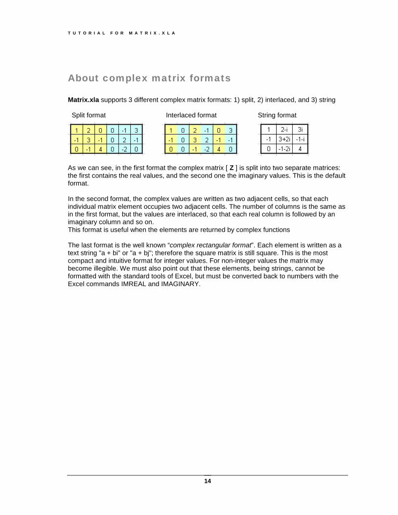
About complex matrix formats Matrix.xla supports 3 different complex matrix formats: 1) split, 2) interlaced, and 3) string Split format Interlaced format String format
As we can see, in the first format the complex matrix [ Z ] is split into two separate matrices: the first contains the real values, and the second one the imaginary values. This is the default format. In the second format, the complex values are written as two adjacent cells, so that each individual matrix element occupies two adjacent cells. The number of columns is the same as in the first format, but the values are interlaced, so that each real column is followed by an imaginary column and so on. This format is useful when the elements are returned by complex functions The last format is the well known “complex rectangular format”. Each element is written as a text string "a + bi" or "a + bj"; therefore the square matrix is still square. This is the most compact and intuitive format for integer values. For non-integer values the matrix may become illegible. We must also point out that these elements, being strings, cannot be formatted with the standard tools of Excel, but must be converted back to numbers with the Excel commands IMREAL and IMAGINARY.

T U T O R I A L F O R M A T R I X . X L A
15
WHITE PAGE
T U T O R I A L F O R M A T R I X . X L A
16
Functions Reference
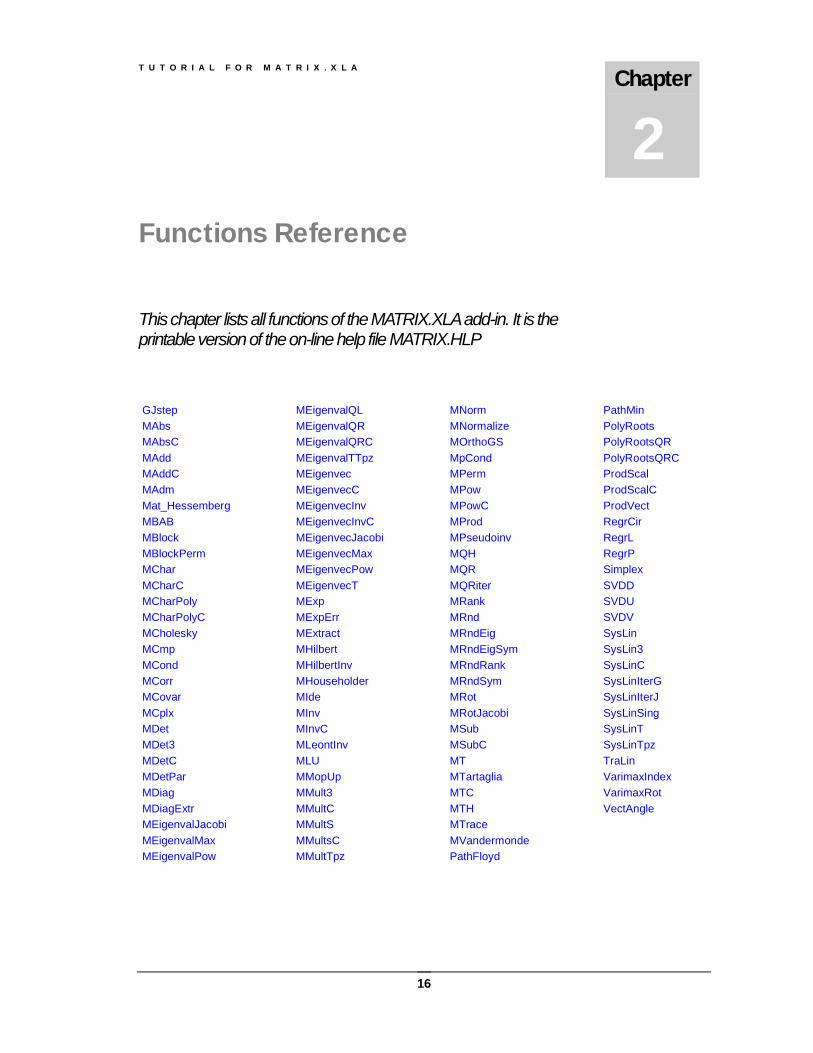
Functions Reference This chapter lists all functions of the MATRIX.XLA add-in. It is the printable version of the on-line help file MATRIX.HLP
GJstep MAbs MAbsC MAdd MAddC MAdm Mat_Hessemberg MBAB MBlock MBlockPerm MChar MCharC MCharPoly MCharPolyC MCholesky MCmp MCond MCorr MCovar MCplx MDet MDet3 MDetC MDetPar MDiag MDiagExtr MEigenvalJacobi MEigenvalMax MEigenvalPow
MEigenvalQL MEigenvalQR MEigenvalQRC MEigenvalTTpz MEigenvec MEigenvecC MEigenvecInv MEigenvecInvC MEigenvecJacobi MEigenvecMax MEigenvecPow MEigenvecT MExp MExpErr MExtract MHilbert MHilbertInv MHouseholder MIde MInv MInvC MLeontInv MLU MMopUp MMult3 MMultC MMultS MMultsC MMultTpz
MNorm MNormalize MOrthoGS MpCond MPerm MPow MPowC MProd MPseudoinv MQH MQR MQRiter MRank MRnd MRndEig MRndEigSym MRndRank MRndSym MRot MRotJacobi MSub MSubC MT MTartaglia MTC MTH MTrace MVandermonde PathFloyd
PathMin PolyRoots PolyRootsQR PolyRootsQRC ProdScal ProdScalC ProdVect RegrCir RegrL RegrP Simplex SVDD SVDU SVDV SysLin SysLin3 SysLinC SysLinIterG SysLinIterJ SysLinSing SysLinT SysLinTpz TraLin VarimaxIndex VarimaxRot VectAngle
Chapter
2
T U T O R I A L F O R M A T R I X . X L A
17
Function MAbs(V) Returns the absolute value ||V|| (Euclidean Norm) of a vector V
∑= 2ivV
The parameter V may be also a matrix; in this case the function returns the Frobenius norm of the matrix
∑= 2ijF
aA
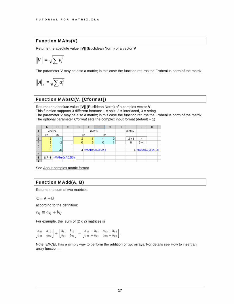
Function MAbsC(V, [Cformat]) Returns the absolute value ||V|| (Euclidean Norm) of a complex vector V This function supports 3 different formats: 1 = split, 2 = interlaced, 3 = string The parameter V may be also a matrix; in this case the function returns the Frobenius norm of the matrix The optional parameter Cformat sets the complex input format (default = 1)
See About complex matrix format
Function MAdd(A, B) Returns the sum of two matrices
according to the definition:
For example, the sum of (2 x 2) matrices is
Note: EXCEL has a simply way to perform the addition of two arrays. For details see How to insert an array function...
T U T O R I A L F O R M A T R I X . X L A
18
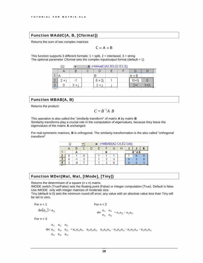
Function MAddC(A, B, [Cformat]) Returns the sum of two complex matrices
This function supports 3 different formats: 1 = split, 2 = interlaced, 3 = string The optional parameter Cformat sets the complex input/output format (default = 1)
Function MBAB(A, B) Returns the product:
BABC 1−= This operation is also called the "similarity transform" of matrix A by matrix B Similarity transforms play a crucial role in the computation of eigenvalues, because they leave the eigenvalues of the matrix A unchanged. For real symmetric matrices, B is orthogonal. The similarity transformation is the also called "orthogonal transform"
Function MDet(Mat, Mat, [IMode], [Tiny]) Returns the determinant of a square (n x n) matrix. IMODE switch (True/False) sets the floating point (False) or integer computation (True). Default is false. Use IMODE only with integer matrices of moderate size. Tiny (default is 0) sets the minimum round-off error; any value with an absolute value less than Tiny will be set to zero.
For n = 1
[ ] 1111det aa =
For n = 2
12212211
2221
1211det aaaaaaaa
−=
For n = 3
122133233211132231322113122331332211
333231
232221
131211
det aaaaaaaaaaaaaaaaaaaaaaaaaaa
−−−++=
T U T O R I A L F O R M A T R I X . X L A
19
Clearly, the computation of the determinant of a large matrix is one of the most tedious of all Math. Fortunately we have Numeric Calculus...! Example - The following matrix is singular, but only the integer computation can give the exact answer
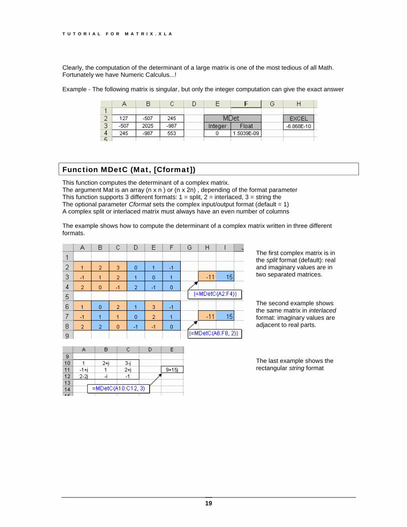
Function MDetC (Mat, [Cformat]) This function computes the determinant of a complex matrix. The argument Mat is an array (n x n ) or (n x 2n) , depending of the format parameter This function supports 3 different formats: 1 = split, 2 = interlaced, 3 = string the The optional parameter Cformat sets the complex input/output format (default = 1) A complex split or interlaced matrix must always have an even number of columns The example shows how to compute the determinant of a complex matrix written in three different formats.
The first complex matrix is in the split format (default): real and imaginary values are in two separated matrices. The second example shows the same matrix in interlaced format: imaginary values are adjacent to real parts. The last example shows the rectangular string format
T U T O R I A L F O R M A T R I X . X L A
20
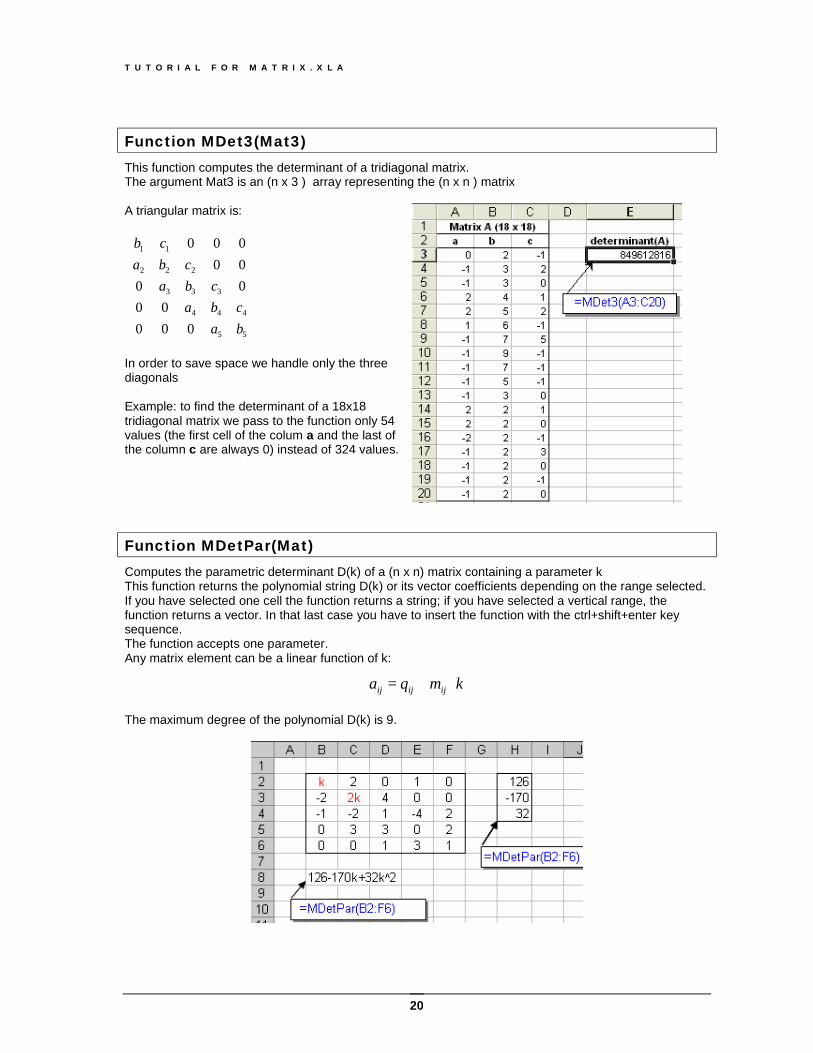
Function MDet3(Mat3) This function computes the determinant of a tridiagonal matrix. The argument Mat3 is an (n x 3 ) array representing the (n x n ) matrix A triangular matrix is:
55
444
333
222
11
00000
0000000
bacba
cbacba
cb
In order to save space we handle only the three diagonals Example: to find the determinant of a 18x18 tridiagonal matrix we pass to the function only 54 values (the first cell of the colum a and the last of the column c are always 0) instead of 324 values.
Function MDetPar(Mat) Computes the parametric determinant D(k) of a (n x n) matrix containing a parameter k This function returns the polynomial string D(k) or its vector coefficients depending on the range selected. If you have selected one cell the function returns a string; if you have selected a vertical range, the function returns a vector. In that last case you have to insert the function with the ctrl+shift+enter key sequence. The function accepts one parameter. Any matrix element can be a linear function of k:
kmqa ijijij ⋅+= The maximum degree of the polynomial D(k) is 9.
T U T O R I A L F O R M A T R I X . X L A
21
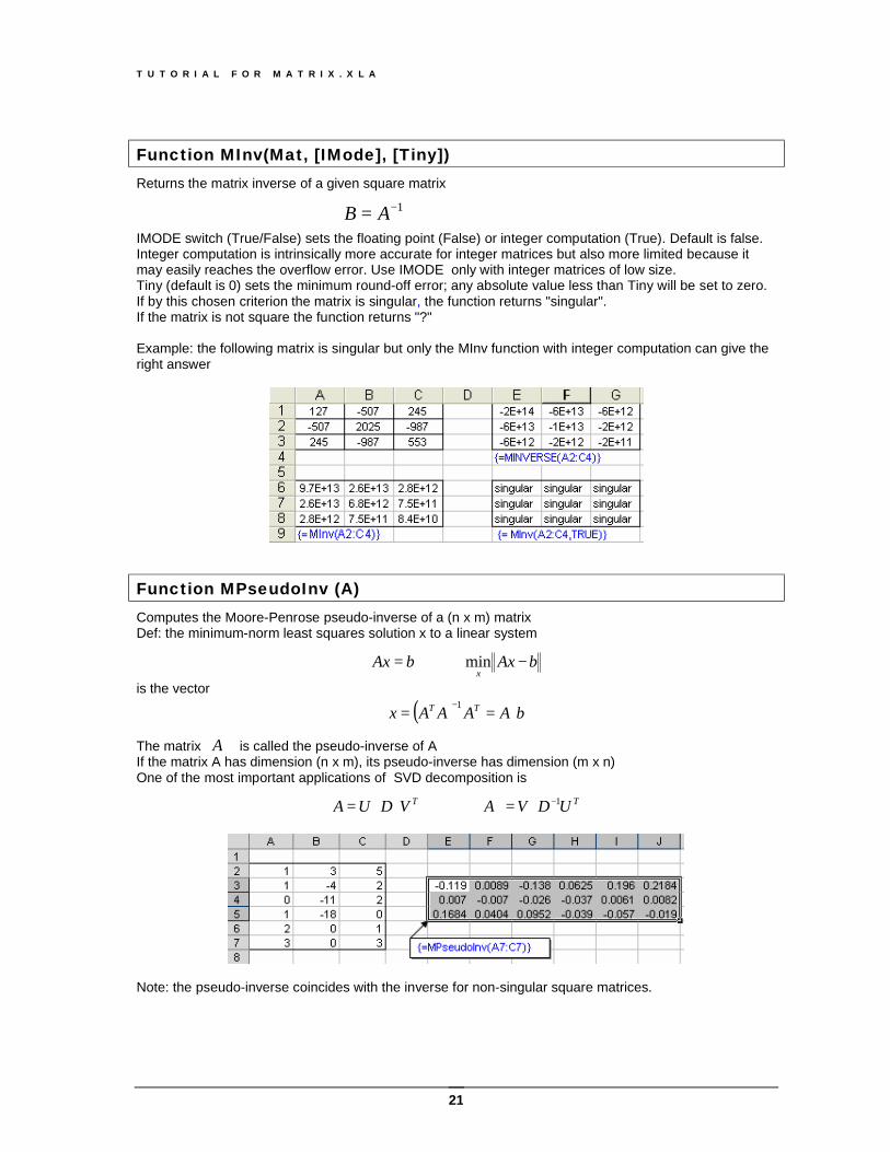
Function MInv(Mat, [IMode], [Tiny]) Returns the matrix inverse of a given square matrix
1−= AB
IMODE switch (True/False) sets the floating point (False) or integer computation (True). Default is false. Integer computation is intrinsically more accurate for integer matrices but also more limited because it may easily reaches the overflow error. Use IMODE only with integer matrices of low size. Tiny (default is 0) sets the minimum round-off error; any absolute value less than Tiny will be set to zero. If by this chosen criterion the matrix is singular, the function returns "singular". If the matrix is not square the function returns "?" Example: the following matrix is singular but only the MInv function with integer computation can give the right answer
Function MPseudoInv (A) Computes the Moore-Penrose pseudo-inverse of a (n x m) matrix Def: the minimum-norm least squares solution x to a linear system
bAxbAxx
−⇒= min
is the vector
( ) bAAAAx TT +−==
1
The matrix +A is called the pseudo-inverse of A If the matrix A has dimension (n x m), its pseudo-inverse has dimension (m x n) One of the most important applications of SVD decomposition is
TVDUA ⋅⋅= ⇒ TUDVA 1−+ ⋅=
Note: the pseudo-inverse coincides with the inverse for non-singular square matrices.
T U T O R I A L F O R M A T R I X . X L A
22
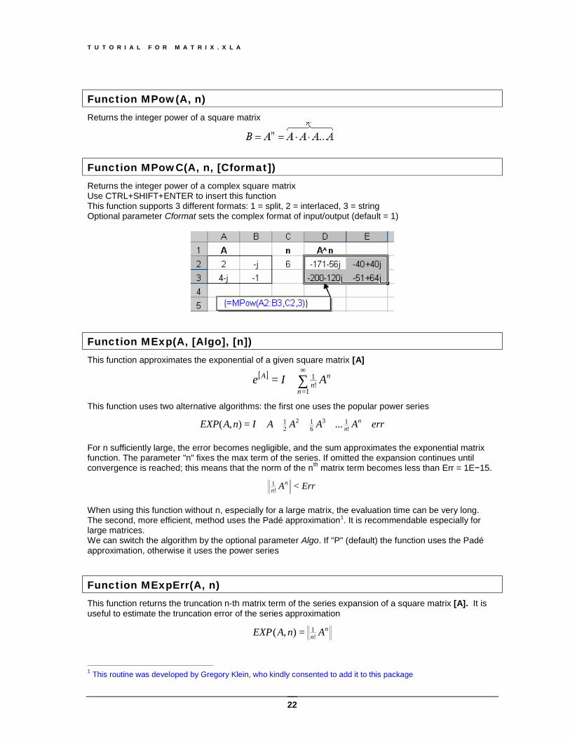
Function MPow(A, n) Returns the integer power of a square matrix
Function MPowC(A, n, [Cformat]) Returns the integer power of a complex square matrix Use CTRL+SHIFT+ENTER to insert this function This function supports 3 different formats: 1 = split, 2 = interlaced, 3 = string Optional parameter Cformat sets the complex format of input/output (default = 1)
Function MExp(A, [Algo], [n]) This function approximates the exponential of a given square matrix [A]
[ ] ∑∞
=+=
1!
1
n
nn
A AIe
This function uses two alternative algorithms: the first one uses the popular power series
errAAAAInAEXP nn +++++= !13
612
21 ...),(
For n sufficiently large, the error becomes negligible, and the sum approximates the exponential matrix function. The parameter "n" fixes the max term of the series. If omitted the expansion continues until convergence is reached; this means that the norm of the nth matrix term becomes less than Err = 1E−15.
ErrAnn <!1
When using this function without n, especially for a large matrix, the evaluation time can be very long. The second, more efficient, method uses the Padé approximation1. It is recommendable especially for large matrices. We can switch the algorithm by the optional parameter Algo. If "P" (default) the function uses the Padé approximation, otherwise it uses the power series
Function MExpErr(A, n) This function returns the truncation n-th matrix term of the series expansion of a square matrix [A]. It is useful to estimate the truncation error of the series approximation
nn AnAEXP !1),( =
1 This routine was developed by Gregory Klein, who kindly consented to add it to this package
T U T O R I A L F O R M A T R I X . X L A
23
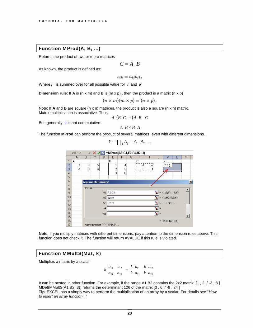
Function MProd(A, B, ...) Returns the product of two or more matrices
BAC ⋅= As known, the product is defined as:
Where j is summed over for all possible value for i and k Dimension rule: If A is (n x m) and B is (m x p) , then the product is a matrix (n x p)
Note: If A and B are square (n x n) matrices, the product is also a square (n x n) matrix. Matrix multiplication is associative. Thus:
( ) ( ) CBACBA ⋅⋅=⋅⋅ But, generally, it is not commutative:
ABBA ⋅≠⋅ The function MProd can perform the product of several matrices, even with different dimensions.
...21 ⋅⋅== ∏ AAAY j j
Note. If you multiply matrices with different dimensions, pay attention to the dimension rules above. This function does not check it. The function will return #VALUE if this rule is violated.
Function MMultS(Mat, k) Multiplies a matrix by a scalar
⋅⋅⋅⋅
=
2221
1211
2221
1211
akakakak
aaaa
k
It can be nested in other function. For example, if the range A1:B2 contains the 2x2 matrix [1 , 2, / -3 , 8 ] MDet(MMultS(A1:B2; 3)) returns the determinant 126 of the matrix [3 , 6, / -9 , 24 ] Tip: EXCEL has a simply way to perform the multiplication of an array by a scalar. For details see "How to insert an array function..."
T U T O R I A L F O R M A T R I X . X L A
24
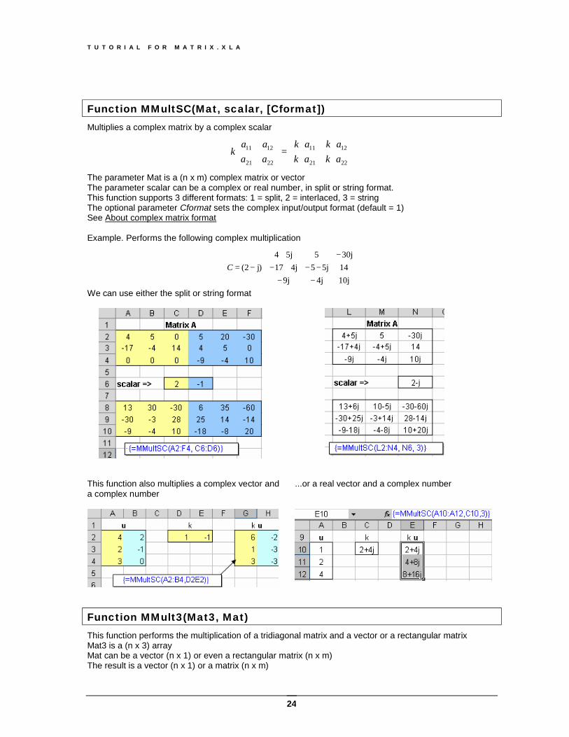
Function MMultSC(Mat, scalar, [Cformat]) Multiplies a complex matrix by a complex scalar
⋅⋅⋅⋅
=
2221
1211
2221
1211
akakakak
aaaa
k
The parameter Mat is a (n x m) complex matrix or vector The parameter scalar can be a complex or real number, in split or string format. This function supports 3 different formats: 1 = split, 2 = interlaced, 3 = string The optional parameter Cformat sets the complex input/output format (default = 1) See About complex matrix format Example. Performs the following complex multiplication
−−−−+−
−+⋅−=
10j4j9j145j54j1730j55j4
)j2(C
We can use either the split or string format
This function also multiplies a complex vector and a complex number
...or a real vector and a complex number
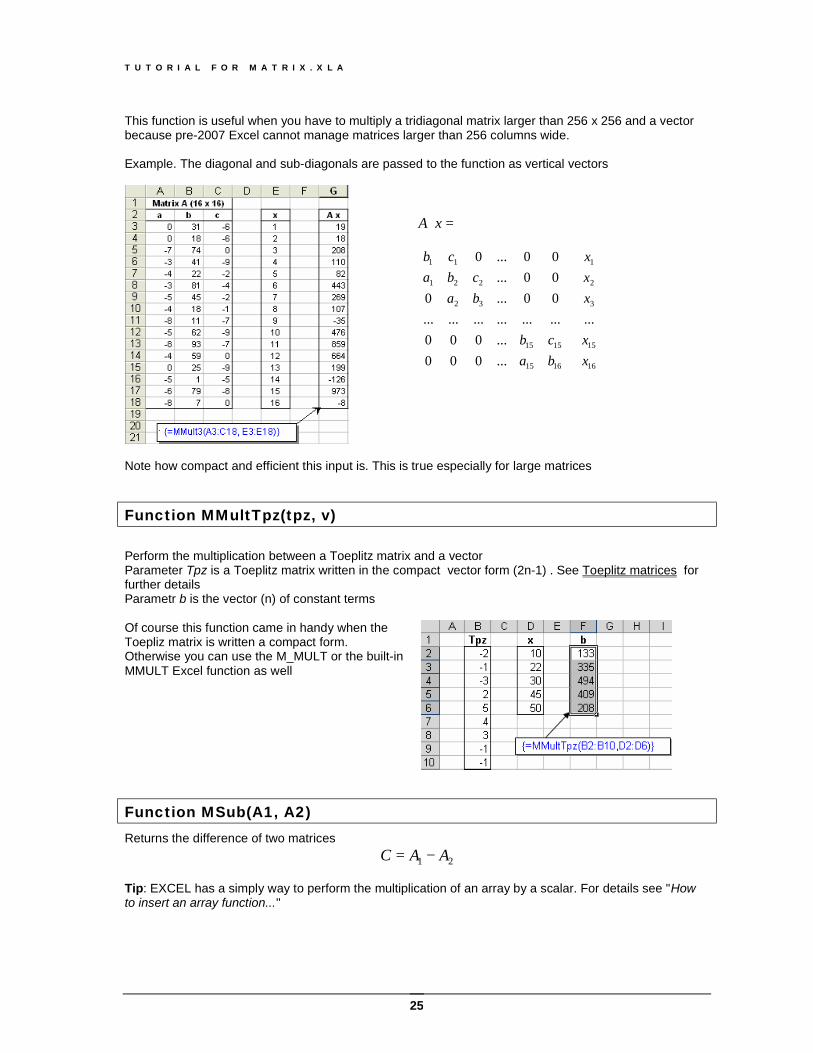
Function MMult3(Mat3, Mat) This function performs the multiplication of a tridiagonal matrix and a vector or a rectangular matrix Mat3 is a (n x 3) array Mat can be a vector (n x 1) or even a rectangular matrix (n x m) The result is a vector (n x 1) or a matrix (n x m)
T U T O R I A L F O R M A T R I X . X L A
25
This function is useful when you have to multiply a tridiagonal matrix larger than 256 x 256 and a vector because pre-2007 Excel cannot manage matrices larger than 256 columns wide. Example. The diagonal and sub-diagonals are passed to the function as vertical vectors
=⋅ xA
⋅
16
15
3
2
1
1615
1515
32
221
11
...
...000
...000..................00...000...00...0
xx
xxx
bacb
bacba
cb
Note how compact and efficient this input is. This is true especially for large matrices
Function MMultTpz(tpz, v) Perform the multiplication between a Toeplitz matrix and a vector Parameter Tpz is a Toeplitz matrix written in the compact vector form (2n-1) . See Toeplitz matrices for further details Parametr b is the vector (n) of constant terms Of course this function came in handy when the Toepliz matrix is written a compact form. Otherwise you can use the M_MULT or the built-in MMULT Excel function as well
Function MSub(A1, A2) Returns the difference of two matrices
21 AAC −= Tip: EXCEL has a simply way to perform the multiplication of an array by a scalar. For details see "How to insert an array function..."
T U T O R I A L F O R M A T R I X . X L A
26
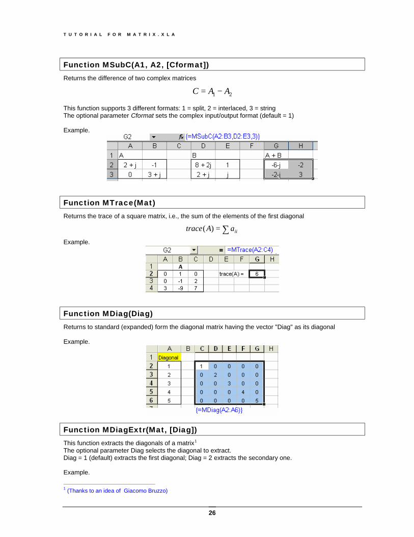
Function MSubC(A1, A2, [Cformat]) Returns the difference of two complex matrices
21 AAC −= This function supports 3 different formats: 1 = split, 2 = interlaced, 3 = string The optional parameter Cformat sets the complex input/output format (default = 1) Example.
Function MTrace(Mat) Returns the trace of a square matrix, i.e., the sum of the elements of the first diagonal
∑= iiaAtrace )( Example.
Function MDiag(Diag) Returns to standard (expanded) form the diagonal matrix having the vector "Diag" as its diagonal Example.
Function MDiagExtr(Mat, [Diag]) This function extracts the diagonals of a matrix1 The optional parameter Diag selects the diagonal to extract. Diag = 1 (default) extracts the first diagonal; Diag = 2 extracts the secondary one. Example.
1 (Thanks to an idea of Giacomo Bruzzo)
T U T O R I A L F O R M A T R I X . X L A
27
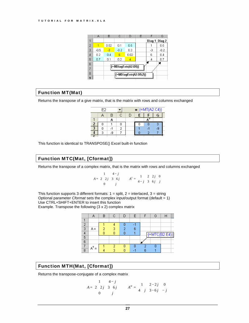
Function MT(Mat) Returns the transpose of a give matrix, that is the matrix with rows and columns exchanged
This function is identical to TRANSPOSE() Excel built-in function
Function MTC(Mat, [Cformat]) Returns the transpose of a complex matrix, that is the matrix with rows and columns exchanged
+−+
=⇒
++−
=jjj
jA
jjjj
A T
6340221
0
632241
This function supports 3 different formats: 1 = split, 2 = interlaced, 3 = string Optional parameter Cformat sets the complex input/output format (default = 1) Use CTRL+SHIFT+ENTER to insert this function Example. Transpose the following (3 x 2) complex matrix
Function MTH(Mat, [Cformat]) Returns the transpose-conjugate of a complex matrix
−−+
−=⇒
++−
=jjj
jA
jjjj
A H
6340221
0
632241
T U T O R I A L F O R M A T R I X . X L A
28
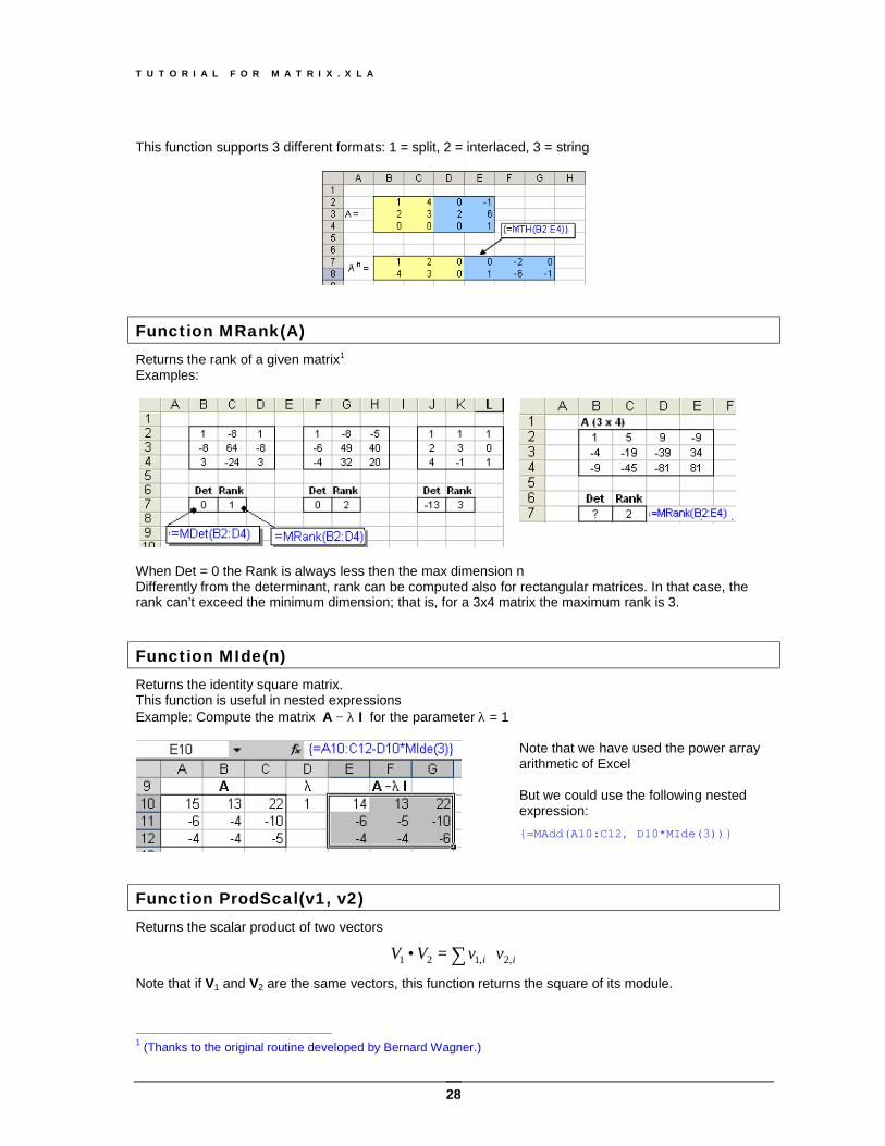
This function supports 3 different formats: 1 = split, 2 = interlaced, 3 = string
Function MRank(A) Returns the rank of a given matrix1 Examples:
When Det = 0 the Rank is always less then the max dimension n Differently from the determinant, rank can be computed also for rectangular matrices. In that case, the rank can’t exceed the minimum dimension; that is, for a 3x4 matrix the maximum rank is 3.
Function MIde(n) Returns the identity square matrix. This function is useful in nested expressions Example: Compute the matrix A − λ I for the parameter λ = 1
Note that we have used the power array arithmetic of Excel But we could use the following nested expression: {=MAdd(A10:C12, D10*MIde(3))}
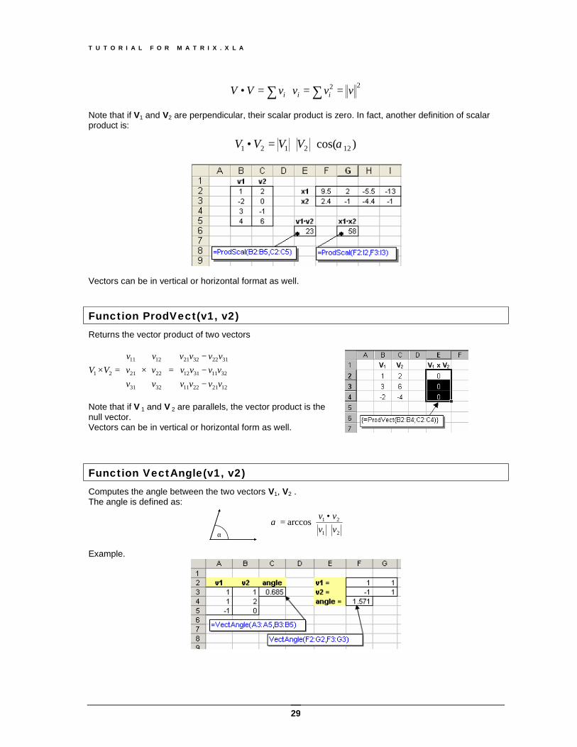
Function ProdScal(v1, v2) Returns the scalar product of two vectors
ii vvVV ,2,121 ⋅=• ∑ Note that if V1 and V2 are the same vectors, this function returns the square of its module.
1 (Thanks to the original routine developed by Bernard Wagner.)
T U T O R I A L F O R M A T R I X . X L A
29
22 vvvvVV iii ==⋅=• ∑∑ Note that if V1 and V2 are perpendicular, their scalar product is zero. In fact, another definition of scalar product is:
)cos( 122121 α⋅⋅=• VVVV
Vectors can be in vertical or horizontal format as well.
Function ProdVect(v1, v2) Returns the vector product of two vectors
−−−
=
×
=×
12212211
32113112
31223221
32
22
12
31
21
11
21
vvvvvvvvvvvv
vvv
vvv
VV
Note that if V 1 and V 2 are parallels, the vector product is the null vector. Vectors can be in vertical or horizontal form as well.
Function VectAngle(v1, v2) Computes the angle between the two vectors V1, V2 . The angle is defined as:
⋅•
=21
21arccosvvvv
α
Example.
α
T U T O R I A L F O R M A T R I X . X L A
30
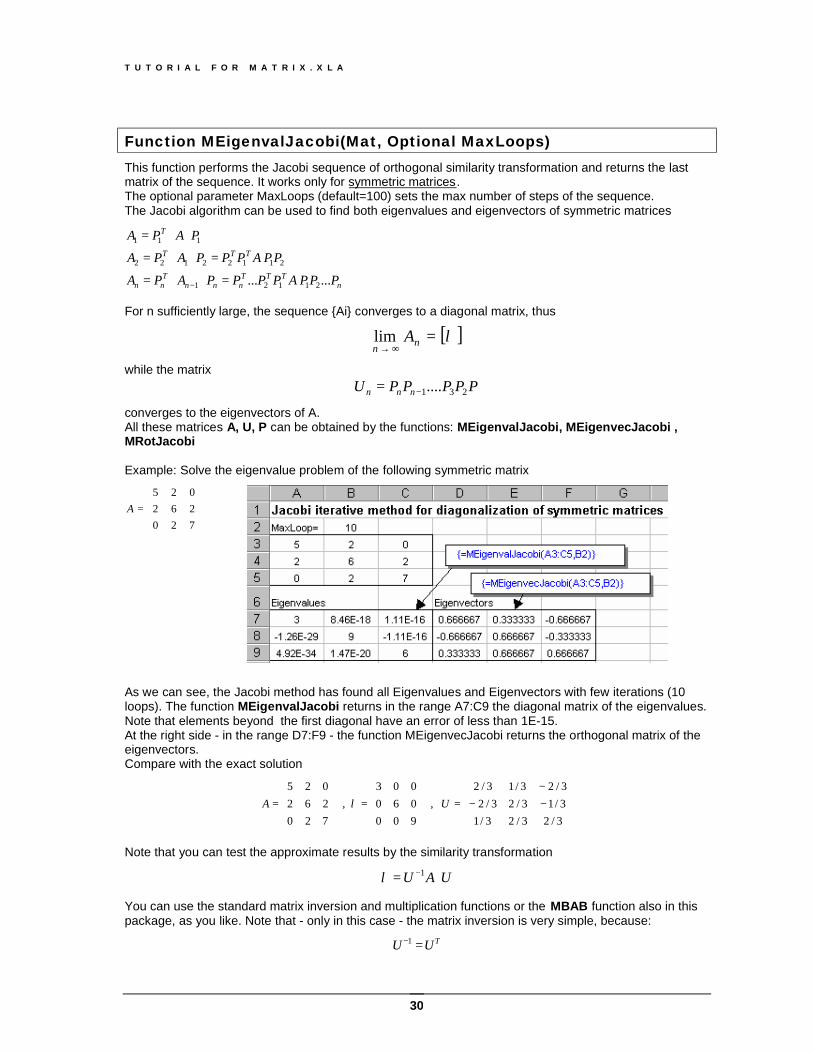
Function MEigenvalJacobi(Mat, Optional MaxLoops) This function performs the Jacobi sequence of orthogonal similarity transformation and returns the last matrix of the sequence. It works only for symmetric matrices. The optional parameter MaxLoops (default=100) sets the max number of steps of the sequence. The Jacobi algorithm can be used to find both eigenvalues and eigenvectors of symmetric matrices
nTTT
nnnT
nn
TTT
T
PPPAPPPPAPA
PPAPPPAPA
PAPA
... ...
21121
21122122
111
=⋅⋅=
=⋅⋅=
⋅⋅=
− For n sufficiently large, the sequence {Ai} converges to a diagonal matrix, thus
[ ]λ=∞→ nn
Alim
while the matrix PPPPPU nnn 231....−=
converges to the eigenvectors of A. All these matrices A, U, P can be obtained by the functions: MEigenvalJacobi, MEigenvecJacobi , MRotJacobi Example: Solve the eigenvalue problem of the following symmetric matrix
=
720262025
A
As we can see, the Jacobi method has found all Eigenvalues and Eigenvectors with few iterations (10 loops). The function MEigenvalJacobi returns in the range A7:C9 the diagonal matrix of the eigenvalues. Note that elements beyond the first diagonal have an error of less than 1E-15. At the right side - in the range D7:F9 - the function MEigenvecJacobi returns the orthogonal matrix of the eigenvectors. Compare with the exact solution
−−−
=
=
=
3/23/23/13/13/23/23/23/13/2
, 900060003
, 720262025
UA λ
Note that you can test the approximate results by the similarity transformation
UAU ⋅= −1λ You can use the standard matrix inversion and multiplication functions or the MBAB function also in this package, as you like. Note that - only in this case - the matrix inversion is very simple, because:
TUU =−1
T U T O R I A L F O R M A T R I X . X L A
31
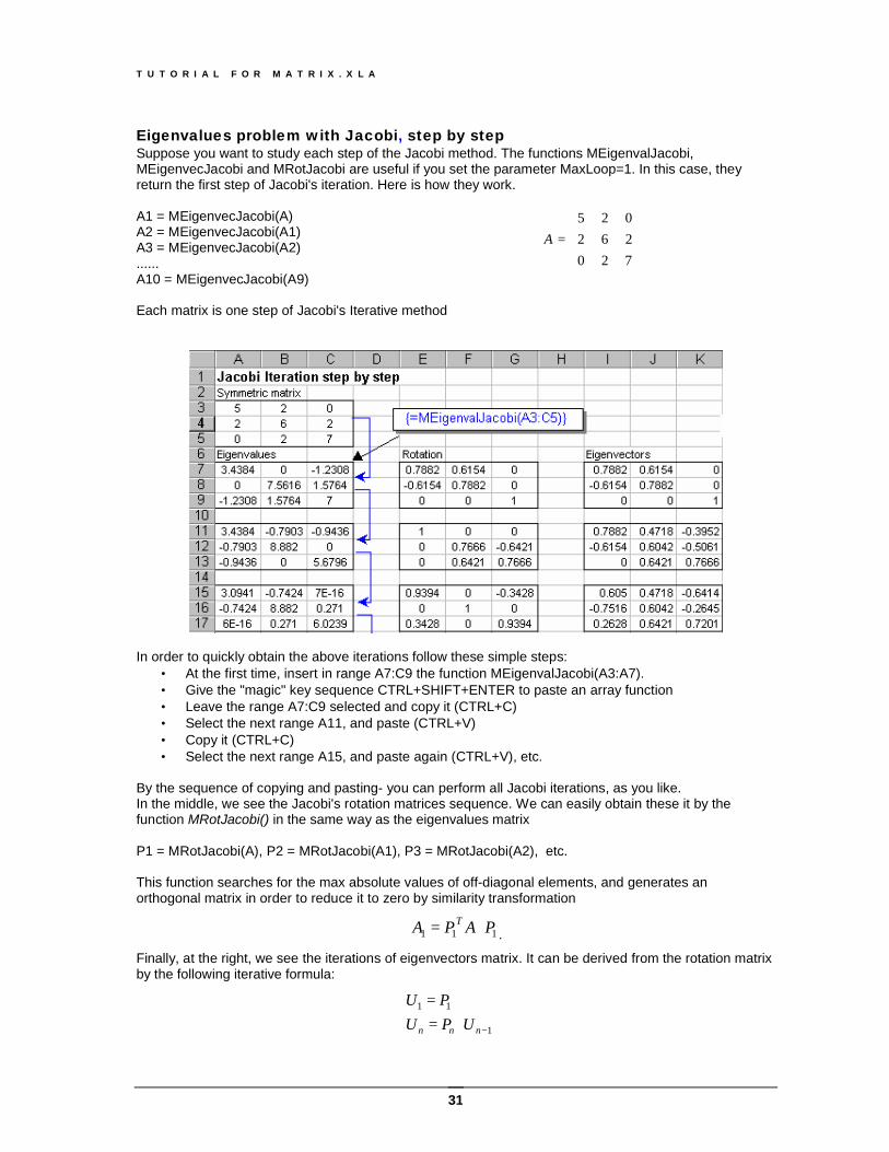
Eigenvalues problem with Jacobi, step by step Suppose you want to study each step of the Jacobi method. The functions MEigenvalJacobi, MEigenvecJacobi and MRotJacobi are useful if you set the parameter MaxLoop=1. In this case, they return the first step of Jacobi's iteration. Here is how they work. A1 = MEigenvecJacobi(A) A2 = MEigenvecJacobi(A1) A3 = MEigenvecJacobi(A2) ...... A10 = MEigenvecJacobi(A9) Each matrix is one step of Jacobi's Iterative method
=
720262025
A
In order to quickly obtain the above iterations follow these simple steps:
• At the first time, insert in range A7:C9 the function MEigenvalJacobi(A3:A7). • Give the "magic" key sequence CTRL+SHIFT+ENTER to paste an array function • Leave the range A7:C9 selected and copy it (CTRL+C) • Select the next range A11, and paste (CTRL+V) • Copy it (CTRL+C) • Select the next range A15, and paste again (CTRL+V), etc.
By the sequence of copying and pasting- you can perform all Jacobi iterations, as you like. In the middle, we see the Jacobi's rotation matrices sequence. We can easily obtain these it by the function MRotJacobi() in the same way as the eigenvalues matrix P1 = MRotJacobi(A), P2 = MRotJacobi(A1), P3 = MRotJacobi(A2), etc. This function searches for the max absolute values of off-diagonal elements, and generates an orthogonal matrix in order to reduce it to zero by similarity transformation
111 PAPA T ⋅= .
Finally, at the right, we see the iterations of eigenvectors matrix. It can be derived from the rotation matrix by the following iterative formula:
1
11
−⋅==
nnn UPUPU
T U T O R I A L F O R M A T R I X . X L A
32
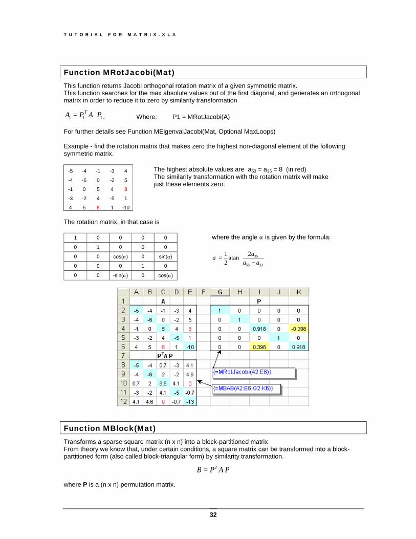
Function MRotJacobi(Mat) This function returns Jacobi orthogonal rotation matrix of a given symmetric matrix. This function searches for the max absolute values out of the first diagonal, and generates an orthogonal matrix in order to reduce it to zero by similarity transformation
111 PAPA T ⋅= . Where: P1 = MRotJacobi(A) For further details see Function MEigenvalJacobi(Mat, Optional MaxLoops) Example - find the rotation matrix that makes zero the highest non-diagonal element of the following symmetric matrix.
-5 -4 -1 -3 4
-4 -6 0 -2 5
-1 0 5 4 8
-3 -2 4 -5 1
4 5 8 1 -10 The rotation matrix, in that case is
1 0 0 0 0
0 1 0 0 0
0 0 cos(α) 0 sin(α)
0 0 0 1 0
0 0 -sin(α) 0 cos(α)
where the angle α is given by the formula:
−
=3355
352atan21
aaa
α
Function MBlock(Mat) Transforms a sparse square matrix (n x n) into a block-partitioned matrix From theory we know that, under certain conditions, a square matrix can be transformed into a block-partitioned form (also called block-triangular form) by similarity transformation.
PAPB T = where P is a (n x n) permutation matrix.
The highest absolute values are a53 = a35 = 8 (in red) The similarity transformation with the rotation matrix will make just these elements zero.
T U T O R I A L F O R M A T R I X . X L A
33
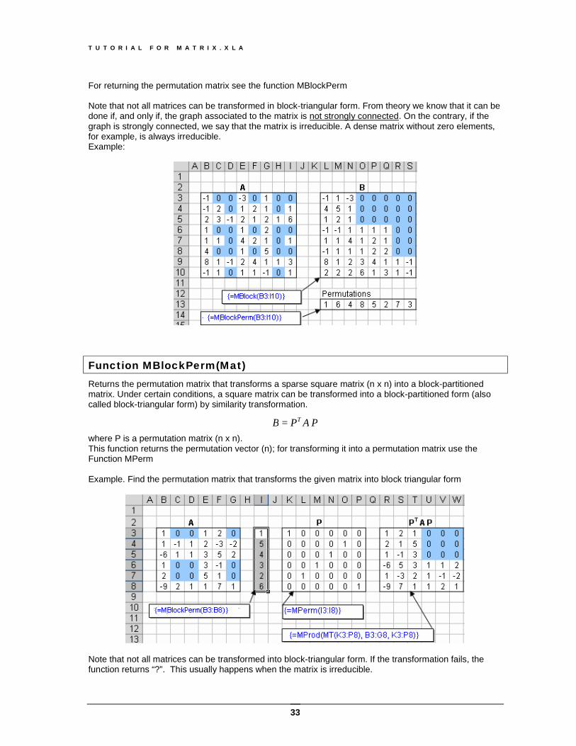
For returning the permutation matrix see the function MBlockPerm Note that not all matrices can be transformed in block-triangular form. From theory we know that it can be done if, and only if, the graph associated to the matrix is not strongly connected. On the contrary, if the graph is strongly connected, we say that the matrix is irreducible. A dense matrix without zero elements, for example, is always irreducible. Example:
Function MBlockPerm(Mat) Returns the permutation matrix that transforms a sparse square matrix (n x n) into a block-partitioned matrix. Under certain conditions, a square matrix can be transformed into a block-partitioned form (also called block-triangular form) by similarity transformation.
PAPB T = where P is a permutation matrix (n x n). This function returns the permutation vector (n); for transforming it into a permutation matrix use the Function MPerm Example. Find the permutation matrix that transforms the given matrix into block triangular form
Note that not all matrices can be transformed into block-triangular form. If the transformation fails, the function returns “?”. This usually happens when the matrix is irreducible.
T U T O R I A L F O R M A T R I X . X L A
34
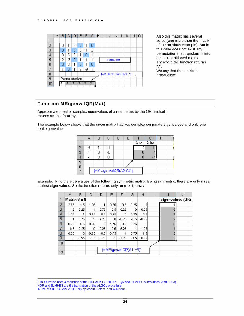
Also this matrix has several zeros (one more then the matrix of the previous example). But in this case does not exist any permutation that transform it into a block-partitioned matrix. Therefore the function returns "?". We say that the matrix is "irreducible"
Function MEigenvalQR(Mat) Approximates real or complex eigenvalues of a real matrix by the QR method1, returns an (n x 2) array The example below shows that the given matrix has two complex conjugate eigenvalues and only one real eigenvalue
Example. Find the eigenvalues of the following symmetric matrix. Being symmetric, there are only n real distinct eigenvalues. So the function returns only an (n x 1) array
1 This function uses a reduction of the EISPACK FORTRAN HQR and ELMHES subroutines (April 1983) HQR and ELMHES are the translation of the ALGOL procedure. NUM. MATH. 14, 219-231(1970) by Martin, Peters, and Wilkinson.
T U T O R I A L F O R M A T R I X . X L A
35
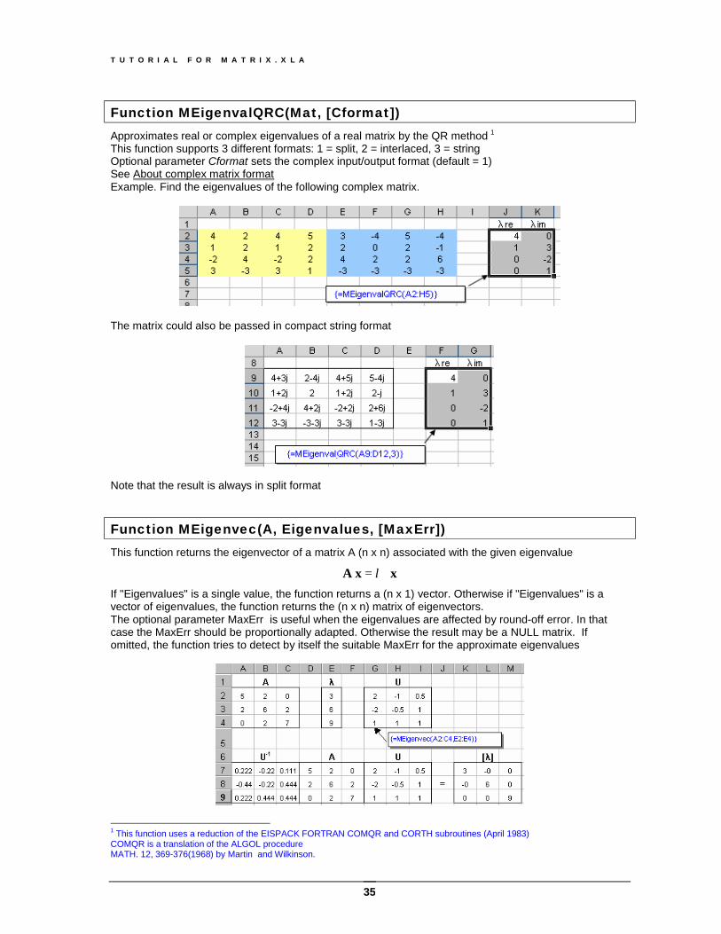
Function MEigenvalQRC(Mat, [Cformat]) Approximates real or complex eigenvalues of a real matrix by the QR method 1 This function supports 3 different formats: 1 = split, 2 = interlaced, 3 = string Optional parameter Cformat sets the complex input/output format (default = 1) See About complex matrix format Example. Find the eigenvalues of the following complex matrix.
The matrix could also be passed in compact string format
Note that the result is always in split format
Function MEigenvec(A, Eigenvalues, [MaxErr]) This function returns the eigenvector of a matrix A (n x n) associated with the given eigenvalue
xx A ⋅= λ
If "Eigenvalues" is a single value, the function returns a (n x 1) vector. Otherwise if "Eigenvalues" is a vector of eigenvalues, the function returns the (n x n) matrix of eigenvectors. The optional parameter MaxErr is useful when the eigenvalues are affected by round-off error. In that case the MaxErr should be proportionally adapted. Otherwise the result may be a NULL matrix. If omitted, the function tries to detect by itself the suitable MaxErr for the approximate eigenvalues
1 This function uses a reduction of the EISPACK FORTRAN COMQR and CORTH subroutines (April 1983) COMQR is a translation of the ALGOL procedure MATH. 12, 369-376(1968) by Martin and Wilkinson.
T U T O R I A L F O R M A T R I X . X L A
36
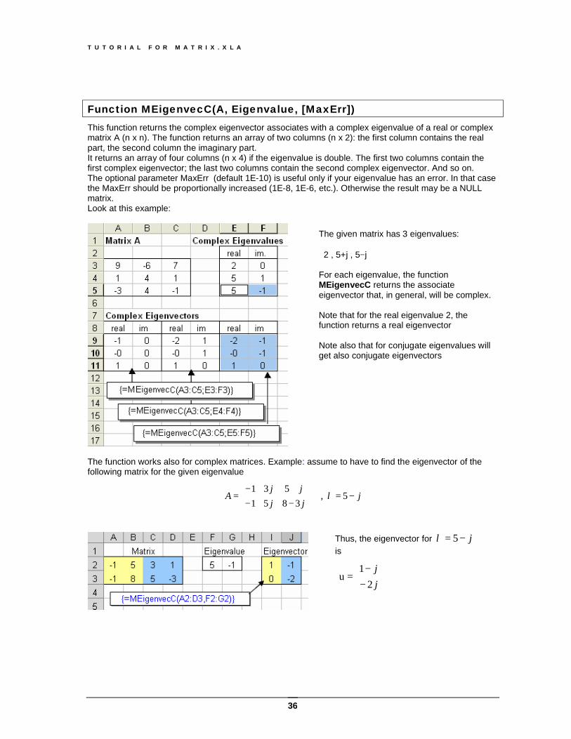
Function MEigenvecC(A, Eigenvalue, [MaxErr]) This function returns the complex eigenvector associates with a complex eigenvalue of a real or complex matrix A (n x n). The function returns an array of two columns (n x 2): the first column contains the real part, the second column the imaginary part. It returns an array of four columns (n x 4) if the eigenvalue is double. The first two columns contain the first complex eigenvector; the last two columns contain the second complex eigenvector. And so on. The optional parameter MaxErr (default 1E-10) is useful only if your eigenvalue has an error. In that case the MaxErr should be proportionally increased (1E-8, 1E-6, etc.). Otherwise the result may be a NULL matrix. Look at this example:
The given matrix has 3 eigenvalues: 2 , 5+j , 5−j For each eigenvalue, the function MEigenvecC returns the associate eigenvector that, in general, will be complex. Note that for the real eigenvalue 2, the function returns a real eigenvector Note also that for conjugate eigenvalues will get also conjugate eigenvectors
The function works also for complex matrices. Example: assume to have to find the eigenvector of the following matrix for the given eigenvalue
jjjjj
A −=
−+−++−
= 5 , 3851
531λ
Thus, the eigenvector for j−= 5λ is
−−
=jj
21
u
T U T O R I A L F O R M A T R I X . X L A
37
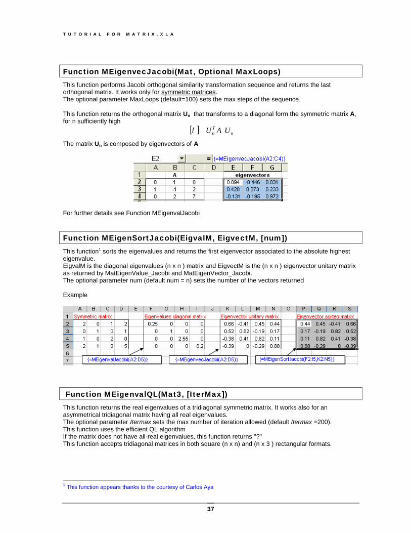
Function MEigenvecJacobi(Mat, Optional MaxLoops) This function performs Jacobi orthogonal similarity transformation sequence and returns the last orthogonal matrix. It works only for symmetric matrices. The optional parameter MaxLoops (default=100) sets the max steps of the sequence. This function returns the orthogonal matrix Un that transforms to a diagonal form the symmetric matrix A, for n sufficiently high
[ ] nTn UAU ⋅≅λ
The matrix Un is composed by eigenvectors of A
For further details see Function MEigenvalJacobi
Function MEigenSortJacobi(EigvalM, EigvectM, [num]) This function1 sorts the eigenvalues and returns the first eigenvector associated to the absolute highest eigenvalue. EigvalM is the diagonal eigenvalues (n x n ) matrix and EigvectM is the (n x n ) eigenvector unitary matrix as returned by MatEigenValue_Jacobi and MatEigenVector_Jacobi. The optional parameter num (default num = n) sets the number of the vectors returned Example
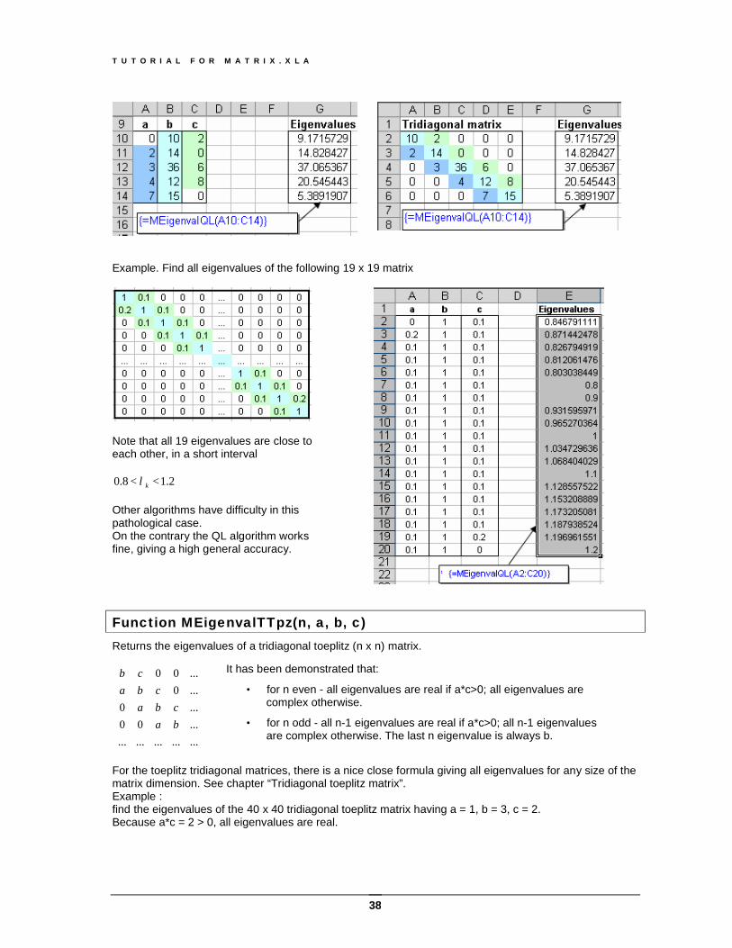
Function MEigenvalQL(Mat3, [IterMax]) This function returns the real eigenvalues of a tridiagonal symmetric matrix. It works also for an asymmetrical tridiagonal matrix having all real eigenvalues. The optional parameter Itermax sets the max number of iteration allowed (default Itermax =200). This function uses the efficient QL algorithm If the matrix does not have all-real eigenvalues, this function returns "?" This function accepts tridiagonal matrices in both square (n x n) and (n x 3 ) rectangular formats.
1 This function appears thanks to the courtesy of Carlos Aya
T U T O R I A L F O R M A T R I X . X L A
38
Example. Find all eigenvalues of the following 19 x 19 matrix
Note that all 19 eigenvalues are close to each other, in a short interval
2.18.0 << kλ Other algorithms have difficulty in this pathological case. On the contrary the QL algorithm works fine, giving a high general accuracy.
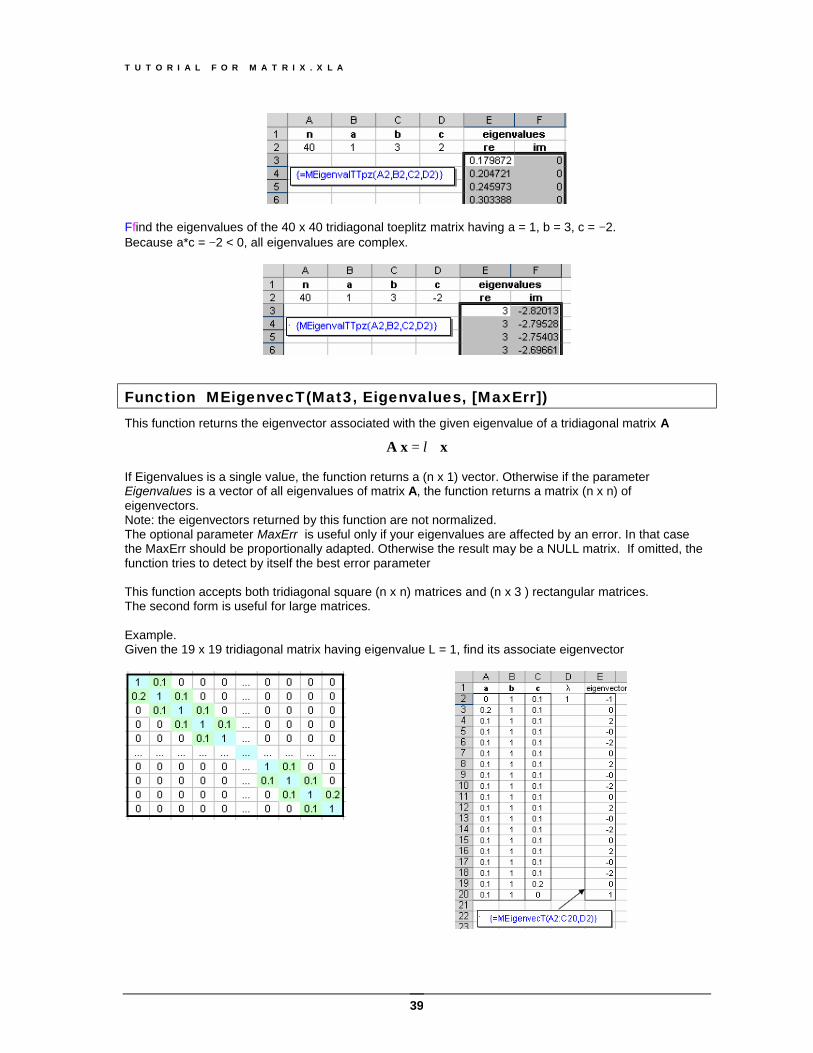
Function MEigenvalTTpz(n, a, b, c) Returns the eigenvalues of a tridiagonal toeplitz (n x n) matrix.
...............
...00
...0
...0
...00
bacba
cbacb
For the toeplitz tridiagonal matrices, there is a nice close formula giving all eigenvalues for any size of the matrix dimension. See chapter “Tridiagonal toeplitz matrix”. Example : find the eigenvalues of the 40 x 40 tridiagonal toeplitz matrix having a = 1, b = 3, c = 2. Because a*c = 2 > 0, all eigenvalues are real.
It has been demonstrated that:
• for n even - all eigenvalues are real if a*c>0; all eigenvalues are complex otherwise.
• for n odd - all n-1 eigenvalues are real if a*c>0; all n-1 eigenvalues are complex otherwise. The last n eigenvalue is always b.
T U T O R I A L F O R M A T R I X . X L A
39
Ffind the eigenvalues of the 40 x 40 tridiagonal toeplitz matrix having a = 1, b = 3, c = −2. Because a*c = −2 < 0, all eigenvalues are complex.
Function MEigenvecT(Mat3, Eigenvalues, [MaxErr]) This function returns the eigenvector associated with the given eigenvalue of a tridiagonal matrix A
xx A ⋅= λ If Eigenvalues is a single value, the function returns a (n x 1) vector. Otherwise if the parameter Eigenvalues is a vector of all eigenvalues of matrix A, the function returns a matrix (n x n) of eigenvectors. Note: the eigenvectors returned by this function are not normalized. The optional parameter MaxErr is useful only if your eigenvalues are affected by an error. In that case the MaxErr should be proportionally adapted. Otherwise the result may be a NULL matrix. If omitted, the function tries to detect by itself the best error parameter This function accepts both tridiagonal square (n x n) matrices and (n x 3 ) rectangular matrices. The second form is useful for large matrices. Example. Given the 19 x 19 tridiagonal matrix having eigenvalue L = 1, find its associate eigenvector
T U T O R I A L F O R M A T R I X . X L A
40
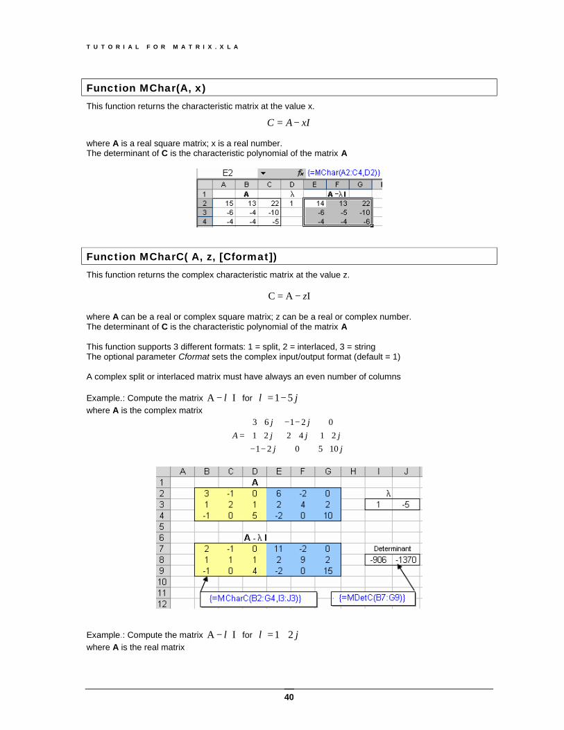
Function MChar(A, x) This function returns the characteristic matrix at the value x.
xIAC −= where A is a real square matrix; x is a real number. The determinant of C is the characteristic polynomial of the matrix A
Function MCharC( A, z, [Cformat]) This function returns the complex characteristic matrix at the value z.
IAC z−= where A can be a real or complex square matrix; z can be a real or complex number. The determinant of C is the characteristic polynomial of the matrix A This function supports 3 different formats: 1 = split, 2 = interlaced, 3 = string The optional parameter Cformat sets the complex input/output format (default = 1) A complex split or interlaced matrix must have always an even number of columns Example.: Compute the matrix I A λ− for j51−=λ where A is the complex matrix
+−−+++
−−+=
jjjjj
jjA
105021214221
02163
Example.: Compute the matrix I A λ− for j21+=λ where A is the real matrix
T U T O R I A L F O R M A T R I X . X L A
41
−
−=
501121013
A
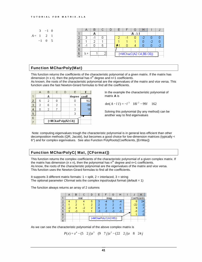
Function MCharPoly(Mat) This function returns the coefficients of the characteristic polynomial of a given matrix. If the matrix has dimension (n x n), then the polynomial has nth degree and n+1 coefficients. As known, the roots of the characteristic polynomial are the eigenvalues of the matrix and vice versa. This function uses the fast Newton-Girard formulas to find all the coefficients.
In the example the characteristic polynomial of matrix A is
1629918)det( 23 +−+−=− λλλλIA Solving this polynomial (by any method) can be another way to find eigenvalues
Note: computing eigenvalues trough the characteristic polynomial is in general less efficient than other decomposition methods (QR, Jacobi), but becomes a good choice for low-dimension matrices (typically < 6°) and for complex eigenvalues. See also Function PolyRoots(Coefficients, [ErrMax])
Function MCharPolyC( Mat, [CFormat]) This function returns the complex coefficients of the characteristic polynomial of a given complex matrix. If the matrix has dimension (n x n), then the polynomial has nth degree and n+1 coefficients. As know, the roots of the characteristic polynomial are the eigenvalues of the matrix and vice versa. This function uses the Newton-Girard formulas to find all the coefficients. It supports 3 different matrix formats: 1 = split, 2 = interlaced, 3 = string The optional parameter Cformat sets the complex input/output format (default = 1) The function always returns an array of 2 columns
As we can see the characteristic polynomial of the above complex matrix is
jzjzjzjzzP 248)222()79()25()( 234 +++−+++−=
T U T O R I A L F O R M A T R I X . X L A
42
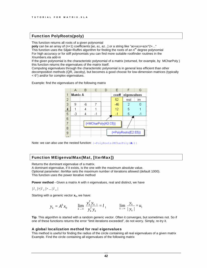
Function PolyRoots(poly) This function returns all roots of a given polynomial poly can be an array of (n+1) coefficients [a0, a1, a2...] or a string like "a0+a1x+a2x^2+..." This function uses the Siljak+Ruffini algorithm for finding the roots of an nth degree polynomial For high accuracy or for stiff polynomials you can find more suitable rootfinder routines in the Xnumbers.xla add-in If the given polynomial is the characteristic polynomial of a matrix (returned, for example, by MCharPoly ) this function returns the eigenvalues of the matrix itself. Computing eigenvalues through the characteristic polynomial is in general less efficient than other decomposition methods (QR, Jacoby), but becomes a good choose for low-dimension matrices (typically < 6°) and/or for complex eigenvalues. Example: find the eigenvalues of the following matrix
Note: we can also use the nested function: {=PolyRoots(MCharPoly(A))}
Function MEigenvalMax(Mat, [IterMax]) Returns the dominant eigenvalue of a matrix. A dominant eigenvalue, if it exists, is the one with the maximum absolute value. Optional parameter: IterMax sets the maximum number of iterations allowed (default 1000). This function uses the power iterative method Power method - Given a matrix A with n eigenvalues, real and distinct, we have
||...|||| 21 nλλλ >> Starting with a generic vector x0, we have: Tip. This algorithm is started with a random generic vector. Often it converges, but sometimes not. So if one of these functions returns the error “limit iterations exceeded”, do not worry. Simply, re-try it. A global localization method for real eigenvalues This method is useful for finding the radius of the circle containing all real eigenvalues of a given matrix Example. Find the circle containing all eigenvalues of the following matrix
11 lim λ=+
∞→k
Tk
kTk
k yyyy
1|| lim u
yy
k
kk
=∞→0xAy k
k =
T U T O R I A L F O R M A T R I X . X L A
43
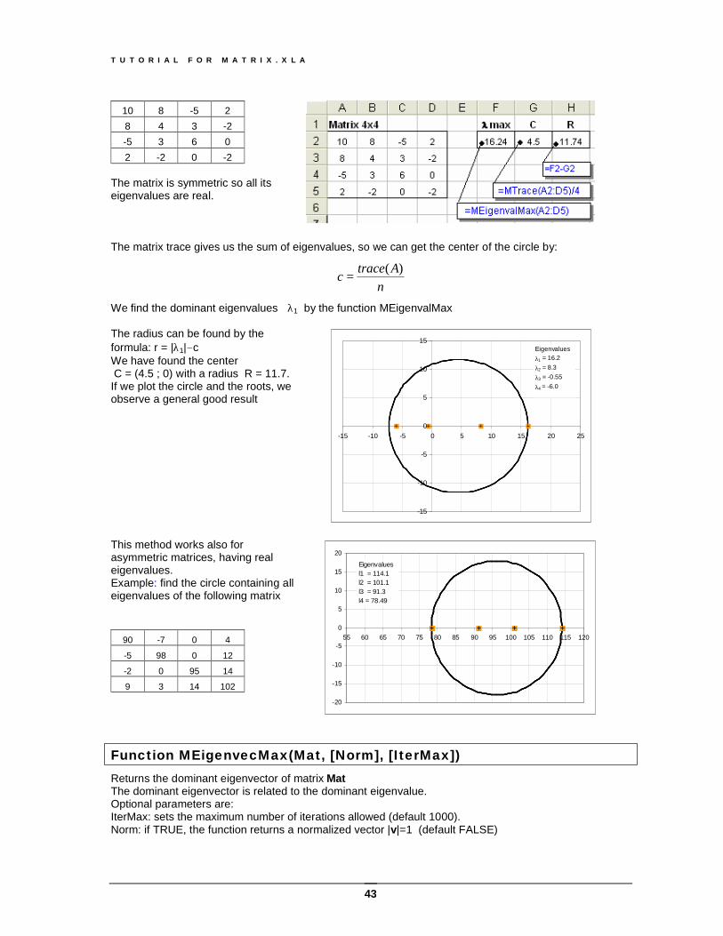
10 8 -5 2 8 4 3 -2 -5 3 6 0 2 -2 0 -2
The matrix is symmetric so all its eigenvalues are real. The matrix trace gives us the sum of eigenvalues, so we can get the center of the circle by:
nAtracec )(
=
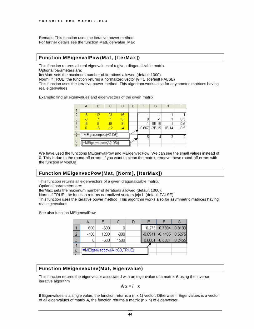
We find the dominant eigenvalues λ1 by the function MEigenvalMax The radius can be found by the formula: r = |λ1|-c We have found the center C = (4.5 ; 0) with a radius R = 11.7. If we plot the circle and the roots, we observe a general good result
-15
-10
-5
0
5
10
15
-15 -10 -5 0 5 10 15 20 25
Eigenvaluesλ1 = 16.2λ2 = 8.3λ3 = -0.55λ4 = -6.0
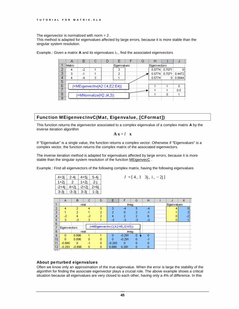
This method works also for asymmetric matrices, having real eigenvalues. Example: find the circle containing all eigenvalues of the following matrix
90 -7 0 4
-5 98 0 12
-2 0 95 14
9 3 14 102 -20
-15
-10
-5
0
5
10
15
20
55 60 65 70 75 80 85 90 95 100 105 110 115 120
Eigenvaluesl1 = 114.1l2 = 101.1l3 = 91.3l4 = 78.49
Function MEigenvecMax(Mat, [Norm], [IterMax]) Returns the dominant eigenvector of matrix Mat The dominant eigenvector is related to the dominant eigenvalue. Optional parameters are: IterMax: sets the maximum number of iterations allowed (default 1000). Norm: if TRUE, the function returns a normalized vector |v|=1 (default FALSE)
T U T O R I A L F O R M A T R I X . X L A
44
Remark: This function uses the iterative power method For further details see the function MatEigenvalue_Max
Function MEigenvalPow(Mat, [IterMax]) This function returns all real eigenvalues of a given diagonalizable matrix. Optional parameters are: IterMax: sets the maximum number of iterations allowed (default 1000). Norm: if TRUE, the function returns a normalized vector |v|=1 (default FALSE) This function uses the iterative power method. This algorithm works also for asymmetric matrices having real eigenvalues Example: find all eigenvalues and eigenvectors of the given matrix
We have used the functions MEigenvalPow and MEigenvecPow. We can see the small values instead of 0. This is due to the round-off errors. If you want to clean the matrix, remove these round-off errors with the function MMopUp
Function MEigenvecPow(Mat, [Norm], [IterMax]) This function returns all eigenvectors of a given diagonalizable matrix. Optional parameters are: IterMax: sets the maximum number of iterations allowed (default 1000). Norm: if TRUE, the function returns normalized vectors |v|=1 (default FALSE) This function uses the iterative power method. This algorithm works also for asymmetric matrices having real eigenvalues See also function MEigenvalPow
Function MEigenvecInv(Mat, Eigenvalue) This function returns the eigenvector associated with an eigenvalue of a matrix A using the inverse iterative algorithm
xx A ⋅= λ If Eigenvalues is a single value, the function returns a (n x 1) vector. Otherwise if Eigenvalues is a vector of all eigenvalues of matrix A, the function returns a matrix (n x n) of eigenvector.
T U T O R I A L F O R M A T R I X . X L A
45
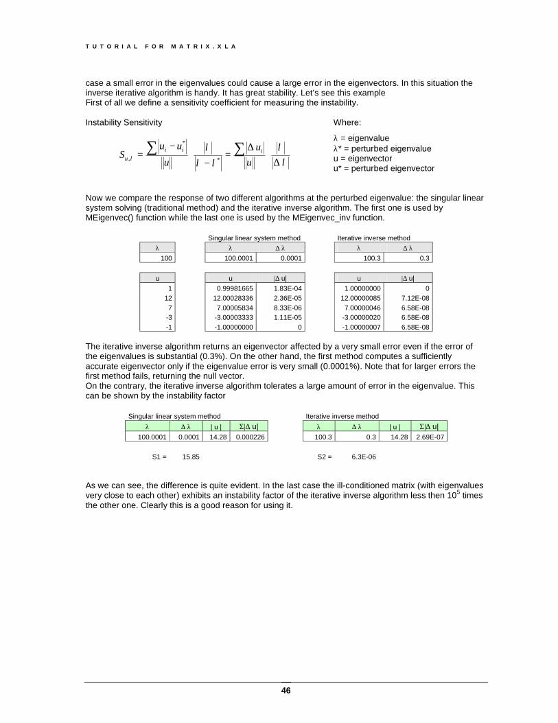
The eigenvector is normalized with norm = 2 . This method is adapted for eigenvalues affected by large errors, because it is more stable than the singular system resolution. Example.: Given a matrix A and its eigenvalues λi , find the associated eigenvectors
Function MEigenvecInvC(Mat, Eigenvalue, [CFormat]) This function returns the eigenvector associated to a complex eigenvalue of a complex matrix A by the inverse iteration algorithm
xx A ⋅= λ If "Eigenvalue" is a single value, the function returns a complex vector. Otherwise if "Eigenvalues" is a complex vector, the function returns the complex matrix of the associated eigenvectors. The inverse iteration method is adapted for eigenvalues affected by large errors, because it is more stable than the singular system resolution of the function MEigenvecC . Example.: Find all eigenvectors of the following complex matrix, having the following eigenvalues
4+3j 2-4j 4+5j 5-4j 1+2j 2 1+2j 2-j -2+4j 4+2j -2+2j 2+6j 3-3j -3-3j 3-3j 1-3j
] 2j , i , 3j1 , 4 [ −+=λ
About perturbed eigenvalues Often we know only an approximation of the true eigenvalue. When the error is large the stability of the algorithm for finding the associate eigenvector plays a crucial role. The above example shows a critical situation because all eigenvalues are very closed to each other, having only a 4% of difference. In this
T U T O R I A L F O R M A T R I X . X L A
46
case a small error in the eigenvalues could cause a large error in the eigenvectors. In this situation the inverse iterative algorithm is handy. It has great stability. Let’s see this example First of all we define a sensitivity coefficient for measuring the instability. Instability Sensitivity
λλ
λλ
λλ
*
*
, ∆⋅
∆=
−⋅
−= ∑∑
uu
uuu
S iiiu
Where:
λ = eigenvalue λ* = perturbed eigenvalue u = eigenvector u* = perturbed eigenvector
Now we compare the response of two different algorithms at the perturbed eigenvalue: the singular linear system solving (traditional method) and the iterative inverse algorithm. The first one is used by MEigenvec() function while the last one is used by the MEigenvec_inv function.
Singular linear system method Iterative inverse method λ λ ∆ λ λ ∆ λ
100 100.0001 0.0001 100.3 0.3
u u |∆ u| u |∆ u| 1 0.99981665 1.83E-04 1.00000000 0
12 12.00028336 2.36E-05 12.00000085 7.12E-08 7 7.00005834 8.33E-06 7.00000046 6.58E-08
-3 -3.00003333 1.11E-05 -3.00000020 6.58E-08 -1 -1.00000000 0 -1.00000007 6.58E-08
The iterative inverse algorithm returns an eigenvector affected by a very small error even if the error of the eigenvalues is substantial (0.3%). On the other hand, the first method computes a sufficiently accurate eigenvector only if the eigenvalue error is very small (0.0001%). Note that for larger errors the first method fails, returning the null vector. On the contrary, the iterative inverse algorithm tolerates a large amount of error in the eigenvalue. This can be shown by the instability factor
Singular linear system method Iterative inverse method λ ∆ λ | u | Σ|∆ u| λ ∆ λ | u | Σ|∆ u|
100.0001 0.0001 14.28 0.000226 100.3 0.3 14.28 2.69E-07
S1 = 15.85 S2 = 6.3E-06 As we can see, the difference is quite evident. In the last case the ill-conditioned matrix (with eigenvalues very close to each other) exhibits an instability factor of the iterative inverse algorithm less then 105 times the other one. Clearly this is a good reason for using it.
T U T O R I A L F O R M A T R I X . X L A
47
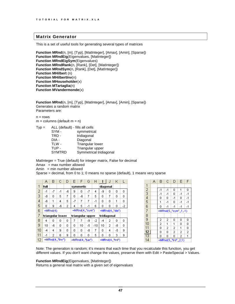
Matrix Generator This is a set of useful tools for generating several types of matrices Function MRnd(n, [m], [Typ], [MatInteger], [Amax], [Amin], [Sparse]) Function MRndEig(Eigenvalues, [MatInteger]) Function MRndEigSym(Eigenvalues) Function MRndRank(n, [Rank], [Det], [MatInteger]) Function MRndSym(n, [Rank], [Det], [MatInteger]) Function MHilbert (n) Function MHilbertInv(n) Function MHouseholder(x) Function MTartaglia(n) Function MVandermonde(x) Function MRnd(n, [m], [Typ], [MatInteger], [Amax], [Amin], [Sparse]) Generates a random matrix Parameters are:
n = rows m = columns (default m = n)
Typ = ALL (default) - fills all cells SYM - symmetrical TRD - tridiagonal DIA - Diagonal TLW - Triangular lower TUP - Triangular upper SYMTRD Symmetrical tridiagonal MatInteger = True (default) for integer matrix, False for decimal Amax = max number allowed Amin = min number allowed Sparse = decimal, from 0 to 1; 0 means no sparse (default), 1 means very sparse
Note: The generation is random; it’s means that each time that you recalculate this function, you get different values. If you don't want change the values, preserve them with Edit > PasteSpecial > Values. Function MRndEig(Eigenvalues, [MatInteger]) Returns a general real matrix with a given set of eigenvalues
T U T O R I A L F O R M A T R I X . X L A
48
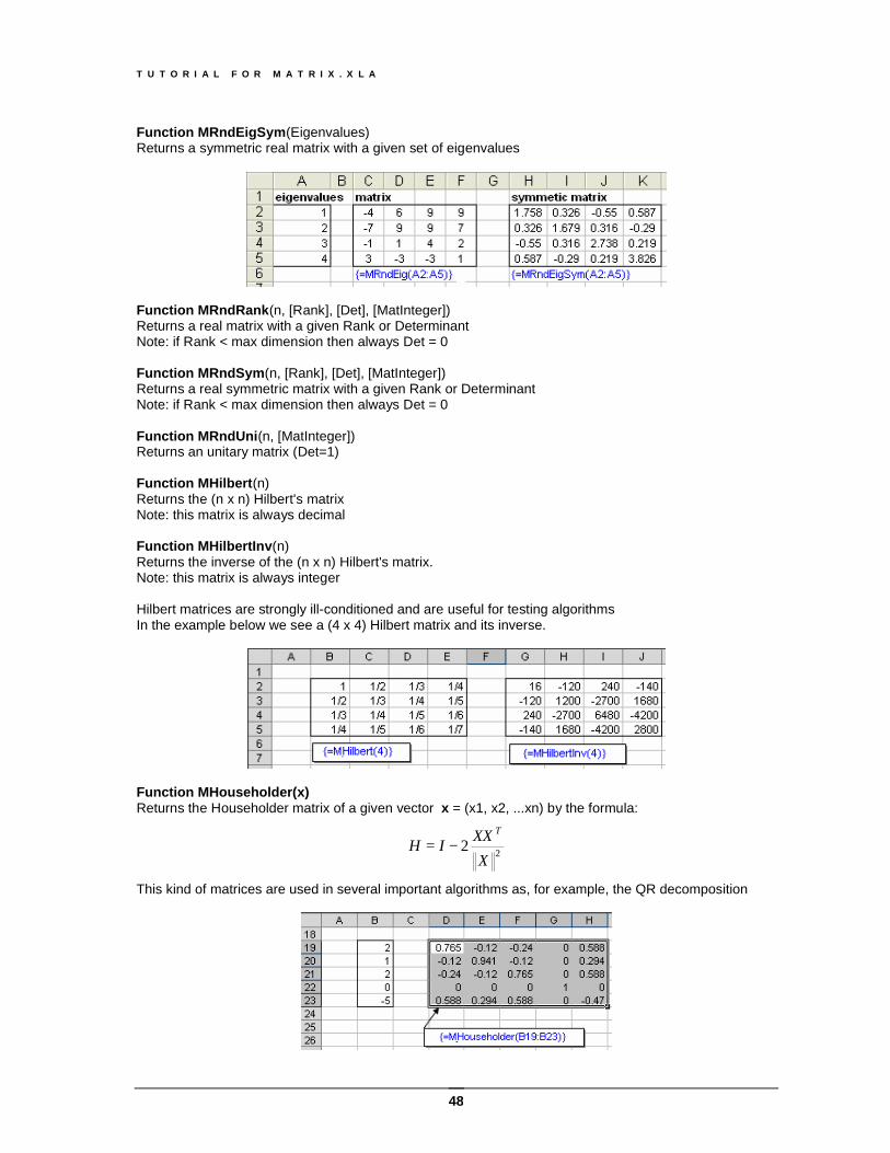
Function MRndEigSym(Eigenvalues) Returns a symmetric real matrix with a given set of eigenvalues
Function MRndRank(n, [Rank], [Det], [MatInteger]) Returns a real matrix with a given Rank or Determinant Note: if Rank < max dimension then always Det = 0 Function MRndSym(n, [Rank], [Det], [MatInteger]) Returns a real symmetric matrix with a given Rank or Determinant Note: if Rank < max dimension then always Det = 0 Function MRndUni(n, [MatInteger]) Returns an unitary matrix (Det=1) Function MHilbert(n) Returns the (n x n) Hilbert's matrix Note: this matrix is always decimal Function MHilbertInv(n) Returns the inverse of the (n x n) Hilbert's matrix. Note: this matrix is always integer Hilbert matrices are strongly ill-conditioned and are useful for testing algorithms In the example below we see a (4 x 4) Hilbert matrix and its inverse.
Function MHouseholder(x) Returns the Householder matrix of a given vector x = (x1, x2, ...xn) by the formula:
22X
XXIHT
−=
This kind of matrices are used in several important algorithms as, for example, the QR decomposition
T U T O R I A L F O R M A T R I X . X L A
49
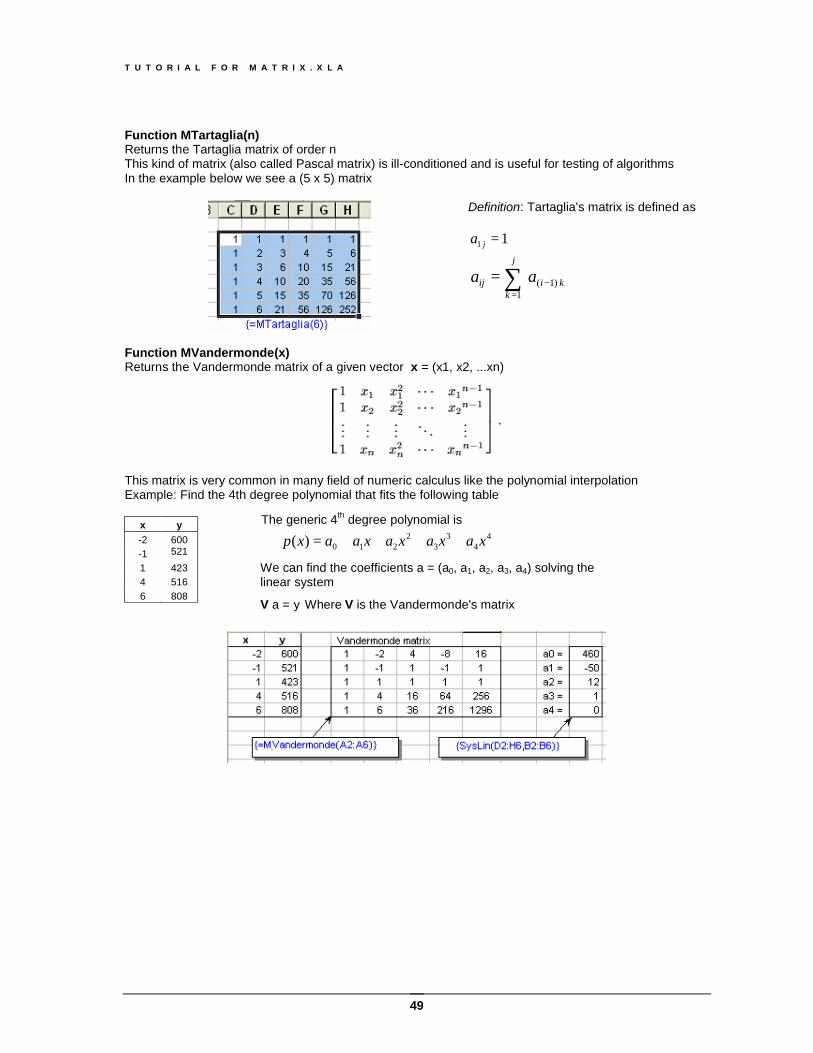
Function MTartaglia(n) Returns the Tartaglia matrix of order n This kind of matrix (also called Pascal matrix) is ill-conditioned and is useful for testing of algorithms In the example below we see a (5 x 5) matrix
Definition: Tartaglia's matrix is defined as
11 =ja
∑=
−=j
kkiij aa
1 )1(
Function MVandermonde(x) Returns the Vandermonde matrix of a given vector x = (x1, x2, ...xn)
This matrix is very common in many field of numeric calculus like the polynomial interpolation Example: Find the 4th degree polynomial that fits the following table
x y -2 600 -1 521 1 423 4 516 6 808
The generic 4th degree polynomial is 4
43
32
210)( xaxaxaxaaxp ++++=
We can find the coefficients a = (a0, a1, a2, a3, a4) solving the linear system
V a = y Where V is the Vandermonde's matrix
T U T O R I A L F O R M A T R I X . X L A
50
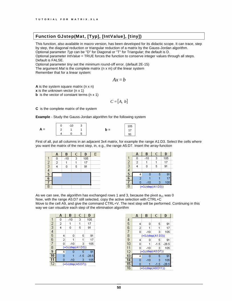
Function GJstep(Mat, [Typ], [IntValue], [tiny]) This function, also available in macro version, has been developed for its didactic scope. It can trace, step by step, the diagonal reduction or triangular reduction of a matrix by the Gauss-Jordan algorithm. Optional parameter Typ can be "D" for Diagonal or "T" for Triangular; the default is D. Optional parameter IntValue = TRUE forces the function to conserve integer values through all steps. Default is FALSE. Optional parameter tiny set the minimum round-off error. (default 2E-15) The argument Mat is the complete matrix (n x m) of the linear system Remember that for a linear system:
bAx = A is the system square matrix (n x n) x is the unknown vector (n x 1) b is the vector of constant terms (n x 1)
[ ]bAC ,= C is the complete matrix of the system Example - Study the Gauss-Jordan algorithm for the following system A = First of all, put all columns in an adjacent 3x4 matrix, for example the range A1:D3. Select the cells where you want the matrix of the next step, in, e.g., the range A5:D7. Insert the array-function
As we can see, the algorithm has exchanged rows 1 and 3, because the pivot a11 was 0 Now, with the range A5:D7 still selected, copy the active selection with CTRL+C Move to the cell A9, and give the command CTRL+V. The next step will be performed. Continuing in this way we can visualize each step of the elimination algorithm
0 -10 3 2 1 1 4 0 5
105 17 91
b =
T U T O R I A L F O R M A T R I X . X L A
51
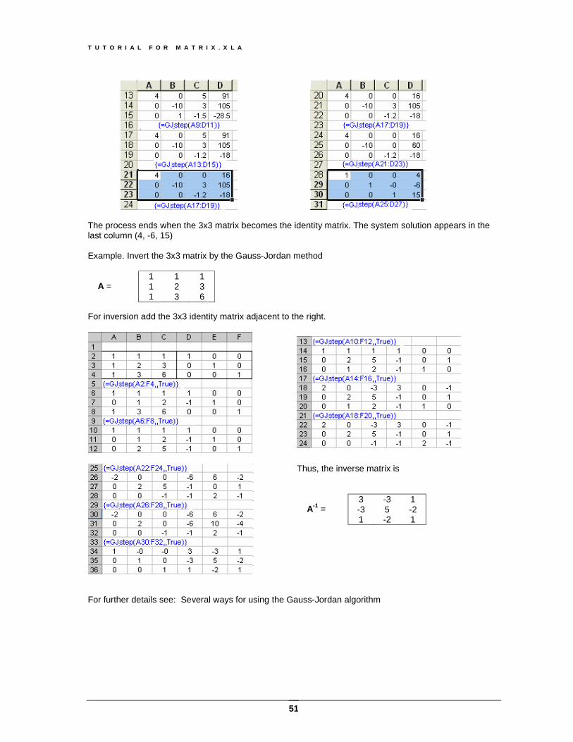
The process ends when the 3x3 matrix becomes the identity matrix. The system solution appears in the last column (4, -6, 15) Example. Invert the 3x3 matrix by the Gauss-Jordan method A = For inversion add the 3x3 identity matrix adjacent to the right.
Thus, the inverse matrix is A-1 =
3 -3 1 -3 5 -2 1 -2 1
For further details see: Several ways for using the Gauss-Jordan algorithm
1 1 1 1 2 3 1 3 6
T U T O R I A L F O R M A T R I X . X L A
52
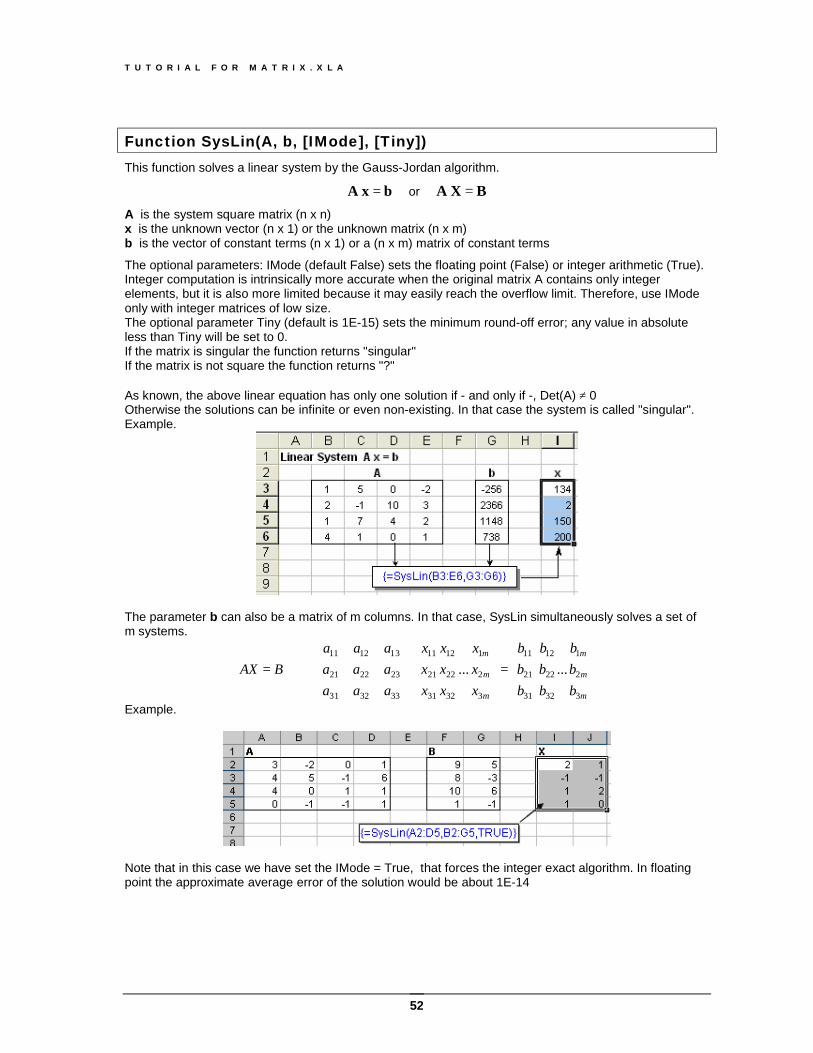
Function SysLin(A, b, [IMode], [Tiny]) This function solves a linear system by the Gauss-Jordan algorithm.
bx A = or BXA =
A is the system square matrix (n x n) x is the unknown vector (n x 1) or the unknown matrix (n x m) b is the vector of constant terms (n x 1) or a (n x m) matrix of constant terms
The optional parameters: IMode (default False) sets the floating point (False) or integer arithmetic (True). Integer computation is intrinsically more accurate when the original matrix A contains only integer elements, but it is also more limited because it may easily reach the overflow limit. Therefore, use IMode only with integer matrices of low size. The optional parameter Tiny (default is 1E-15) sets the minimum round-off error; any value in absolute less than Tiny will be set to 0. If the matrix is singular the function returns "singular" If the matrix is not square the function returns "?" As known, the above linear equation has only one solution if - and only if -, Det(A) ≠ 0 Otherwise the solutions can be infinite or even non-existing. In that case the system is called "singular". Example.
The parameter b can also be a matrix of m columns. In that case, SysLin simultaneously solves a set of m systems.
=
⋅
⇒=
m
m
m
m
m
m
bbb
bbb
bbb
xxx
xxx
xxx
aaaaaaaaa
BAX
3
2
1
32
22
12
31
21
11
3
2
1
32
22
12
31
21
11
33321 3
232221
3 11211
... ...
Example.
Note that in this case we have set the IMode = True, that forces the integer exact algorithm. In floating point the approximate average error of the solution would be about 1E-14
T U T O R I A L F O R M A T R I X . X L A
53
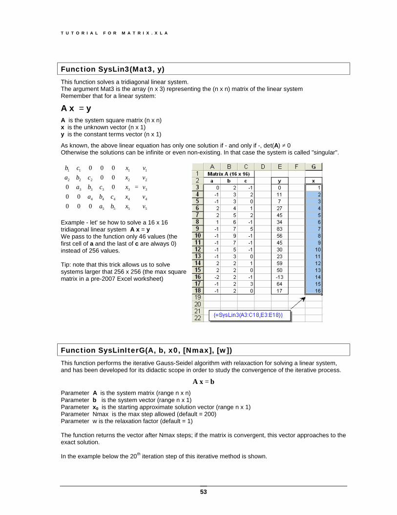
Function SysLin3(Mat3, y) This function solves a tridiagonal linear system. The argument Mat3 is the array (n x 3) representing the (n x n) matrix of the linear system Remember that for a linear system:
A x = y A is the system square matrix (n x n) x is the unknown vector (n x 1) y is the constant terms vector (n x 1)
As known, the above linear equation has only one solution if - and only if -, det(A) ≠ 0 Otherwise the solutions can be infinite or even non-existing. In that case the system is called "singular".
=
⋅
5
4
3
2
1
5
4
3
2
1
55
444
333
222
11
00000
0000000
vvvvv
xxxxx
bacba
cbacba
cb
Example - let' se how to solve a 16 x 16 tridiagonal linear system A x = y We pass to the function only 46 values (the first cell of a and the last of c are always 0) instead of 256 values. Tip: note that this trick allows us to solve systems larger that 256 x 256 (the max square matrix in a pre-2007 Excel worksheet)
Function SysLinIterG(A, b, x0, [Nmax], [w]) This function performs the iterative Gauss-Seidel algorithm with relaxaction for solving a linear system, and has been developed for its didactic scope in order to study the convergence of the iterative process.
bx A =
Parameter A is the system matrix (range n x n) Parameter b is the system vector (range n x 1) Parameter x0 is the starting approximate solution vector (range n x 1) Parameter Nmax is the max step allowed (default = 200) Parameter w is the relaxation factor (default = 1) The function returns the vector after Nmax steps; if the matrix is convergent, this vector approaches to the exact solution. In the example below the 20th iteration step of this iterative method is shown.
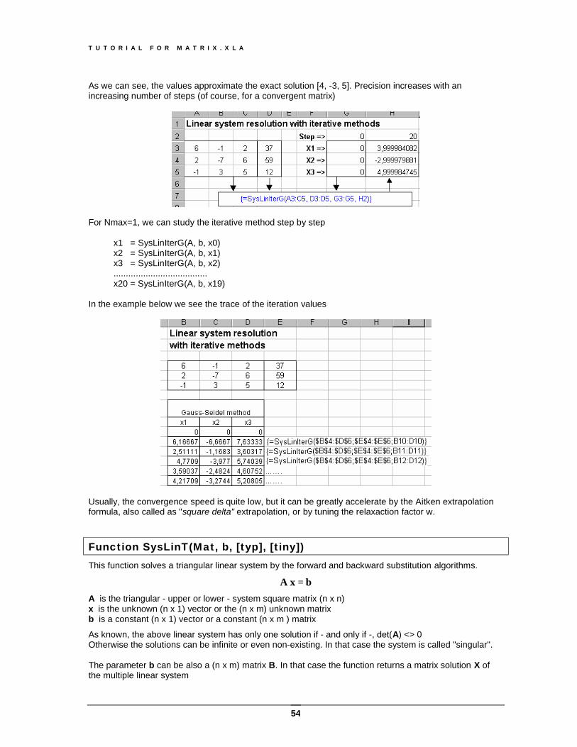
T U T O R I A L F O R M A T R I X . X L A
54
As we can see, the values approximate the exact solution [4, -3, 5]. Precision increases with an increasing number of steps (of course, for a convergent matrix)
For Nmax=1, we can study the iterative method step by step
x1 = SysLinIterG(A, b, x0) x2 = SysLinIterG(A, b, x1) x3 = SysLinIterG(A, b, x2) ...................................... x20 = SysLinIterG(A, b, x19)
In the example below we see the trace of the iteration values
Usually, the convergence speed is quite low, but it can be greatly accelerate by the Aitken extrapolation formula, also called as "square delta" extrapolation, or by tuning the relaxaction factor w.
Function SysLinT(Mat, b, [typ], [tiny]) This function solves a triangular linear system by the forward and backward substitution algorithms.
bx A =
A is the triangular - upper or lower - system square matrix (n x n) x is the unknown (n x 1) vector or the (n x m) unknown matrix b is a constant (n x 1) vector or a constant (n x m ) matrix
As known, the above linear system has only one solution if - and only if -, det(A) <> 0 Otherwise the solutions can be infinite or even non-existing. In that case the system is called "singular". The parameter b can be also a (n x m) matrix B. In that case the function returns a matrix solution X of the multiple linear system
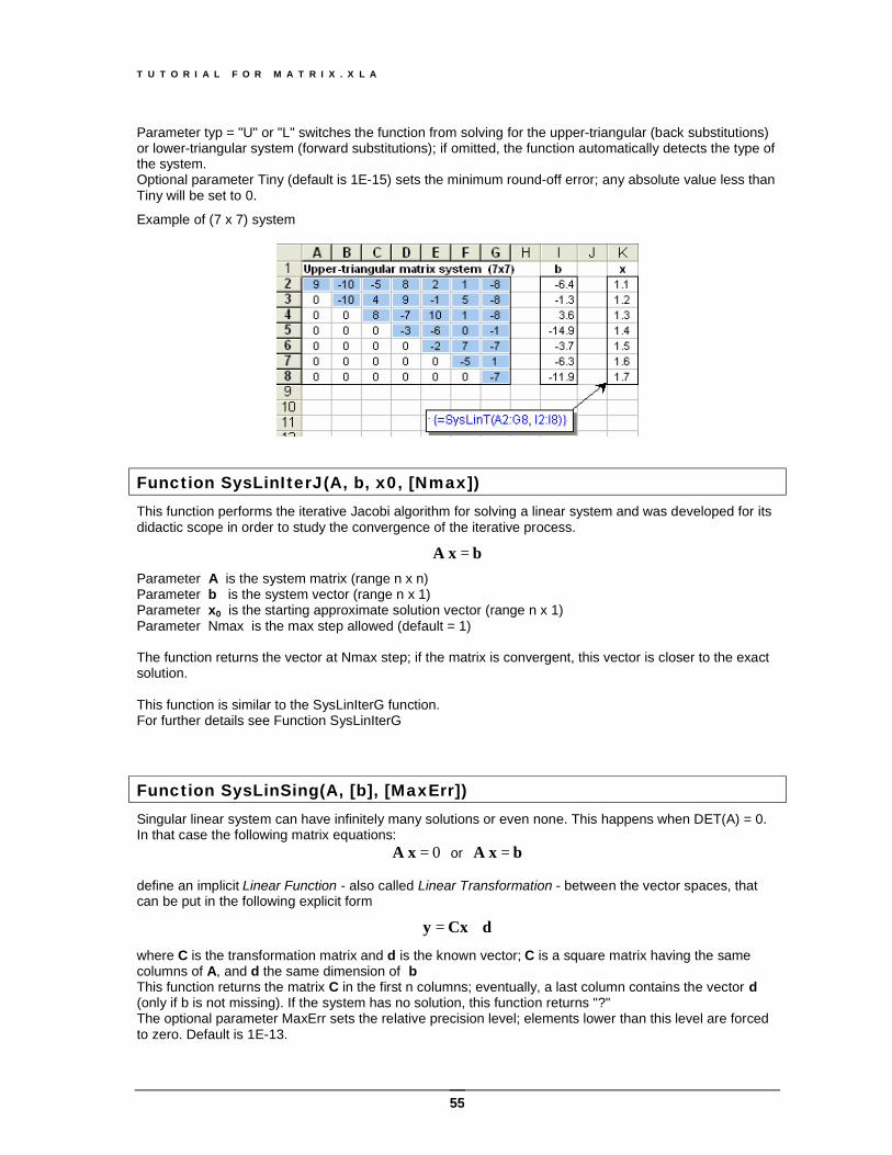
T U T O R I A L F O R M A T R I X . X L A
55
Parameter typ = "U" or "L" switches the function from solving for the upper-triangular (back substitutions) or lower-triangular system (forward substitutions); if omitted, the function automatically detects the type of the system. Optional parameter Tiny (default is 1E-15) sets the minimum round-off error; any absolute value less than Tiny will be set to 0.
Example of (7 x 7) system
Function SysLinIterJ(A, b, x0, [Nmax]) This function performs the iterative Jacobi algorithm for solving a linear system and was developed for its didactic scope in order to study the convergence of the iterative process.
bx A =
Parameter A is the system matrix (range n x n) Parameter b is the system vector (range n x 1) Parameter x0 is the starting approximate solution vector (range n x 1) Parameter Nmax is the max step allowed (default = 1) The function returns the vector at Nmax step; if the matrix is convergent, this vector is closer to the exact solution. This function is similar to the SysLinIterG function. For further details see Function SysLinIterG
Function SysLinSing(A, [b], [MaxErr]) Singular linear system can have infinitely many solutions or even none. This happens when DET(A) = 0. In that case the following matrix equations:
0=x A or bx A = define an implicit Linear Function - also called Linear Transformation - between the vector spaces, that can be put in the following explicit form
dCxy +=
where C is the transformation matrix and d is the known vector; C is a square matrix having the same columns of A, and d the same dimension of b This function returns the matrix C in the first n columns; eventually, a last column contains the vector d (only if b is not missing). If the system has no solution, this function returns "?" The optional parameter MaxErr sets the relative precision level; elements lower than this level are forced to zero. Default is 1E-13.
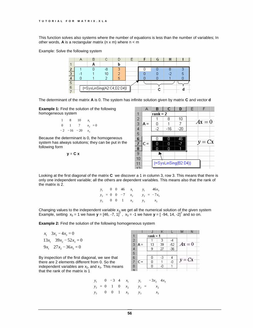
T U T O R I A L F O R M A T R I X . X L A
56
This function solves also systems where the number of equations is less than the number of variables; In other words, A is a rectangular matrix (n x m) where n < m Example: Solve the following system
The determinant of the matrix A is 0. The system has infinite solution given by matrix C and vector d Example 1: Find the solution of the following homogeneous system
020162710
1081
3
2
1
=
⋅
−−− xxx
Because the determinant is 0, the homogeneous system has always solutions; they can be put in the following form
y = C x
Looking at the first diagonal of the matrix C we discover a 1 in column 3, row 3. This means that there is only one independent variable; all the others are dependent variables. This means also that the rank of the matrix is 2.
−=
⇒
⋅
−=
3
3
3
3
2
1
3
2
1
3
2
1
746
100700
4600
xxx
yyy
xxx
yyy
Changing values to the independent variable x3 we get all the numerical solution of the given system Example, setting x3 = 1 we have y = [46, -7, 1]T , x3 = -1 we have y = [ -94, 14, -2]T and so on. Example 2: Find the solution of the following homogeneous system
=−+=−+
=−+
0362790523913
043
321
321
321
xxxxxx
xxx
By inspection of the first diagonal, we see that there are 2 elements different from 0. So the independent variables are x2, and x3. This means that the rank of the matrix is 1
+−=
⇒
⋅
−=
3
2
32
3
2
1
3
2
1
3
2
1 43
100010430
xx
xx
yyy
xxx
yyy
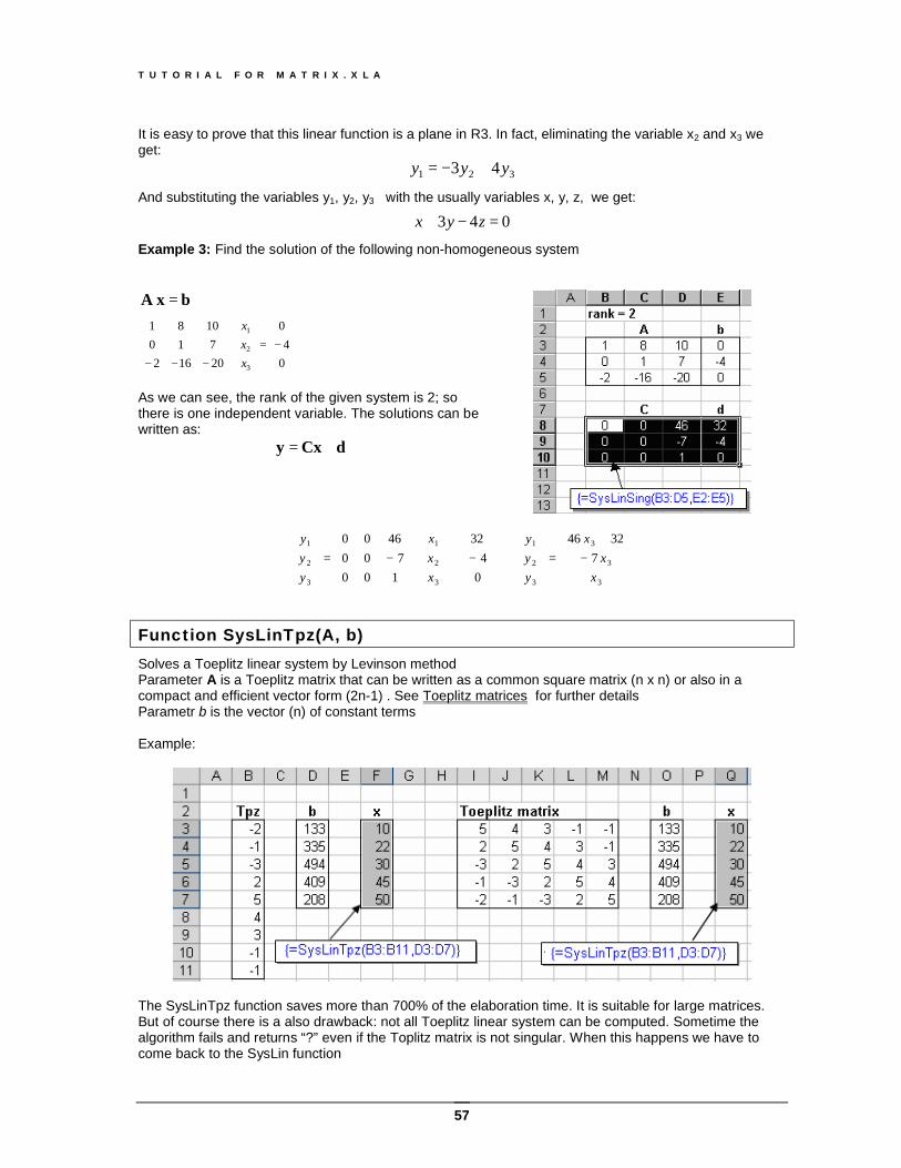
T U T O R I A L F O R M A T R I X . X L A
57
It is easy to prove that this linear function is a plane in R3. In fact, eliminating the variable x2 and x3 we get:
321 43 yyy +−= And substituting the variables y1, y2, y3 with the usually variables x, y, z, we get:
043 =−+ zyx Example 3: Find the solution of the following non-homogeneous system
bx A =
−=
⋅
−−− 04
0
20162710
1081
3
2
1
xxx
As we can see, the rank of the given system is 2; so there is one independent variable. The solutions can be written as:
dCxy +=
−
+=
⇒
−+
⋅
−=
3
3
3
3
2
1
3
2
1
3
2
1
73246
04
32
100700
4600
xx
x
yyy
xxx
yyy
Function SysLinTpz(A, b) Solves a Toeplitz linear system by Levinson method Parameter A is a Toeplitz matrix that can be written as a common square matrix (n x n) or also in a compact and efficient vector form (2n-1) . See Toeplitz matrices for further details Parametr b is the vector (n) of constant terms Example:
The SysLinTpz function saves more than 700% of the elaboration time. It is suitable for large matrices. But of course there is a also drawback: not all Toeplitz linear system can be computed. Sometime the algorithm fails and returns “?” even if the Toplitz matrix is not singular. When this happens we have to come back to the SysLin function
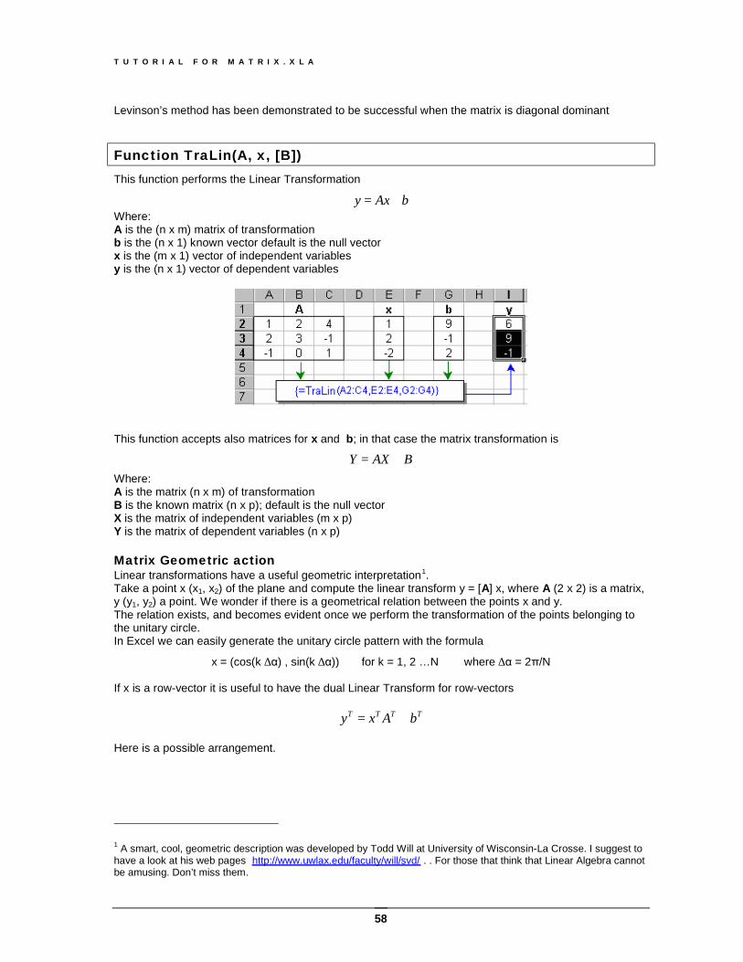
T U T O R I A L F O R M A T R I X . X L A
58
Levinson’s method has been demonstrated to be successful when the matrix is diagonal dominant
Function TraLin(A, x, [B]) This function performs the Linear Transformation
bAxy += Where: A is the (n x m) matrix of transformation b is the (n x 1) known vector default is the null vector x is the (m x 1) vector of independent variables y is the (n x 1) vector of dependent variables
This function accepts also matrices for x and b; in that case the matrix transformation is
BAXY += Where: A is the matrix (n x m) of transformation B is the known matrix (n x p); default is the null vector X is the matrix of independent variables (m x p) Y is the matrix of dependent variables (n x p) Matrix Geometric action Linear transformations have a useful geometric interpretation1. Take a point x (x1, x2) of the plane and compute the linear transform y = [A] x, where A (2 x 2) is a matrix, y (y1, y2) a point. We wonder if there is a geometrical relation between the points x and y. The relation exists, and becomes evident once we perform the transformation of the points belonging to the unitary circle. In Excel we can easily generate the unitary circle pattern with the formula
x = (cos(k⋅∆α) , sin(k⋅∆α)) for k = 1, 2 …N where ∆α = 2π/N If x is a row-vector it is useful to have the dual Linear Transform for row-vectors
TTTT bAxy += Here is a possible arrangement.
1 A smart, cool, geometric description was developed by Todd Will at University of Wisconsin-La Crosse. I suggest to have a look at his web pages http://www.uwlax.edu/faculty/will/svd/ . . For those that think that Linear Algebra cannot be amusing. Don’t miss them.
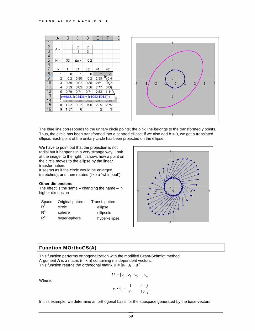
T U T O R I A L F O R M A T R I X . X L A
59
-4
-3
-2
-1
0
1
2
3
4
-4 -3 -2 -1 0 1 2 3 4
The blue line corresponds to the unitary circle points; the pink line belongs to the transformed y points. Thus, the circle has been transformed into a centred ellipse; if we also add b ≠ 0, we get a translated ellipse. Each point of the unitary circle has been projected on the ellipse. We have to point out that the projection is not radial but it happens in a very strange way. Look at the image to the right. It shows how a point on the circle moves to the ellipse by the linear transformation. It seems as if the circle would be enlarged (stretched), and then rotated (like a “whirlpool”). Other dimensions The effect is the same – changing the name – in higher dimension Space Original pattern Transf. pattern R2 circle ⇒ ellipse R3 sphere ⇒ ellipsoid Rn hyper-sphere ⇒ hyper-ellipse
-4
-3
-2
-1
0
1
2
3
4
-4 -2 0 2 4
Function MOrthoGS(A) This function performs orthogonalization with the modified Gram-Schmidt method Argument A is a matrix (m x n) containing n independent vectors. This function returns the orthogonal matrix U = [u1, u2, ..un]
( )nvvvvU ..., , , 321= Where:
≠⇔=⇔
=•jiji
vv ji 0 1
In this example, we determine an orthogonal basis for the subspace generated by the base-vectors
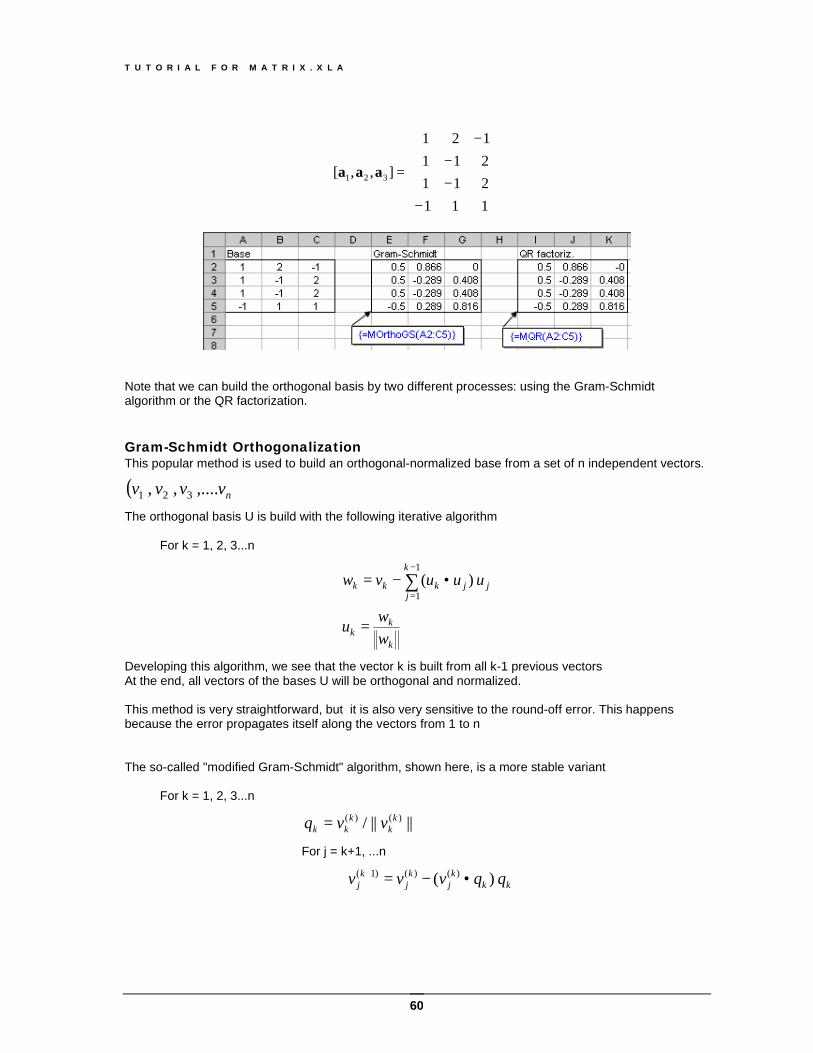
T U T O R I A L F O R M A T R I X . X L A
60
−−−
−
=
1 1 1 2 11 2 11 12 1
],,[ 321 aaa
Note that we can build the orthogonal basis by two different processes: using the Gram-Schmidt algorithm or the QR factorization. Gram-Schmidt Orthogonalization This popular method is used to build an orthogonal-normalized base from a set of n independent vectors.
( )nvvvv ,.... , , 321 The orthogonal basis U is build with the following iterative algorithm
For k = 1, 2, 3...n
k
kk
k
jjjkkk
wwu
uuuvw
=
•−= ∑−
=
1
1 )(
Developing this algorithm, we see that the vector k is built from all k-1 previous vectors At the end, all vectors of the bases U will be orthogonal and normalized. This method is very straightforward, but it is also very sensitive to the round-off error. This happens because the error propagates itself along the vectors from 1 to n The so-called "modified Gram-Schmidt" algorithm, shown here, is a more stable variant
For k = 1, 2, 3...n
||||/ )()( kk
kkk vvq =
For j = k+1, ...n
kkk
jk
jk
j qqvvv )( )()()1( •−=+
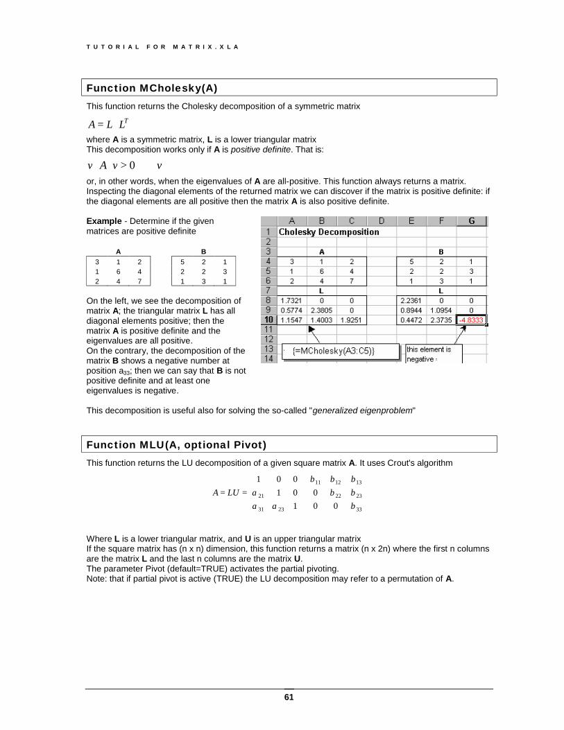
T U T O R I A L F O R M A T R I X . X L A
61
Function MCholesky(A) This function returns the Cholesky decomposition of a symmetric matrix
TLLA ⋅= where A is a symmetric matrix, L is a lower triangular matrix This decomposition works only if A is positive definite. That is:
vvAv ∀>⋅⋅ 0 or, in other words, when the eigenvalues of A are all-positive. This function always returns a matrix. Inspecting the diagonal elements of the returned matrix we can discover if the matrix is positive definite: if the diagonal elements are all positive then the matrix A is also positive definite. Example - Determine if the given matrices are positive definite
A B 3 1 2 5 2 1 1 6 4 2 2 3 2 4 7 1 3 1
On the left, we see the decomposition of matrix A; the triangular matrix L has all diagonal elements positive; then the matrix A is positive definite and the eigenvalues are all positive. On the contrary, the decomposition of the matrix B shows a negative number at position a33; then we can say that B is not positive definite and at least one eigenvalues is negative.
This decomposition is useful also for solving the so-called "generalized eigenproblem"
Function MLU(A, optional Pivot) This function returns the LU decomposition of a given square matrix A. It uses Crout's algorithm
⋅
==
33
2322
131211
2331
21
000
101001
ββββββ
αααLUA
Where L is a lower triangular matrix, and U is an upper triangular matrix If the square matrix has (n x n) dimension, this function returns a matrix (n x 2n) where the first n columns are the matrix L and the last n columns are the matrix U. The parameter Pivot (default=TRUE) activates the partial pivoting. Note: that if partial pivot is active (TRUE) the LU decomposition may refer to a permutation of A.
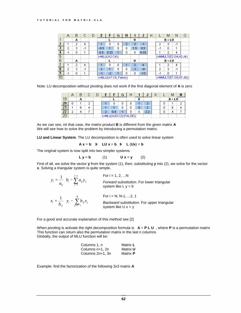
T U T O R I A L F O R M A T R I X . X L A
62
Note: LU decomposition without pivoting does not work if the first diagonal element of A is zero
As we can see, int that case, the matrix product B is different from the given matrix A We will see how to solve the problem by introducing a permutation matrix. LU and Linear System. The LU decomposition is often used to solve linear system
A x = b ⇒ LU x = b ⇒ L (Ux) = b
The original system is now split into two simpler systems.
L y = b (1) U x = y (2)
First of all, we solve the vector y from the system (1), then, substituting y into (2), we solve for the vector x. Solving a triangular system is quite simple. For a good and accurate explanation of this method see [2] When pivoting is activate the right decomposition formula is A = P L U , where P is a permutation matrix This function can return also the permutation matrix in the last n columns Globally, the output of MLU function will be:
Columns 1, n Matrix L Columns n+1, 2n Matrix U Columns 2n+1, 3n Matrix P
Example: find the factorization of the following 3x3 matrix A
−= ∑
−
=
1
1
1 i
jjiji
iii yab
ay
For i = 1, 2, ...N
Forward substitution. For lower triangular system like L y = b
−= ∑
+=
N
ijjiji
iii xyx
1
1β
β
For i = N, N-1, ...2, 1
Backward substitution. For upper triangular system like U x = y
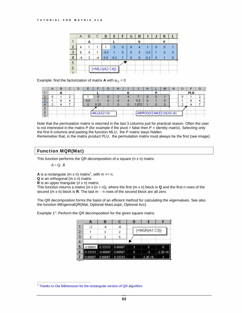
T U T O R I A L F O R M A T R I X . X L A
63
Example: find the factorization of matrix A with a11 = 0
Note that the permutation matrix is returned in the last 3 columns just for practical reason. Often the user is not interested in the matrix P (for example if the pivot = false then P = identity matrix). Selecting only the first 6 columns and pasting the function MLU, the P matrix stays hidden. Rememeber that, in the matrix product PLU, the permutation matrix must always be the first (see image).
Function MQR(Mat) This function performs the QR decomposition of a square (n x n) matrix
RQA ⋅= A is a rectangular (m x n) matrix1, with m >= n. Q is an orthogonal (m x n) matrix R is an upper triangular (n x n) matrix. This function returns a matrix (m x (n + n)), where the first (m x n) block is Q and the first n rows of the second (m x n) block is R. The last m - n rows of the second block are all zero. The QR decomposition forms the basis of an efficient method for calculating the eigenvalues. See also the function MEigenvalQR(Mat, Optional MaxLoops, Optional Acc) Example 1°: Perform the QR decomposition for the given square matrix
1 Thanks to Ola Mårtensson for the rectangular version of QR algorithm
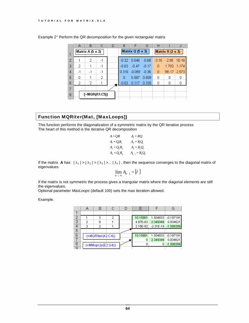
T U T O R I A L F O R M A T R I X . X L A
64
Example 2° Perform the QR decomposition for the given rectangular matrix
Function MQRiter(Mat, [MaxLoops]) This function performs the diagonalization of a symmetric matrix by the QR iterative process The heart of this method is the iterative QR decomposition
nnnnnn QRARQAQRARQAQRARQA
RQAQRA
=⇒==⇒==⇒==⇒=
+1
223222
112111
1
If the matrix A has: | λ1 | > | λ2 | > | λ3 | >... | λn | , then the sequence converges to the diagonal matrix of eigenvalues
[ ]λ=+∞→ 1lim nnA
If the matrix is not symmetric the process gives a triangular matrix where the diagonal elements are still the eigenvalues. Optional parameter MaxLoops (default 100) sets the max iteration allowed. Example.
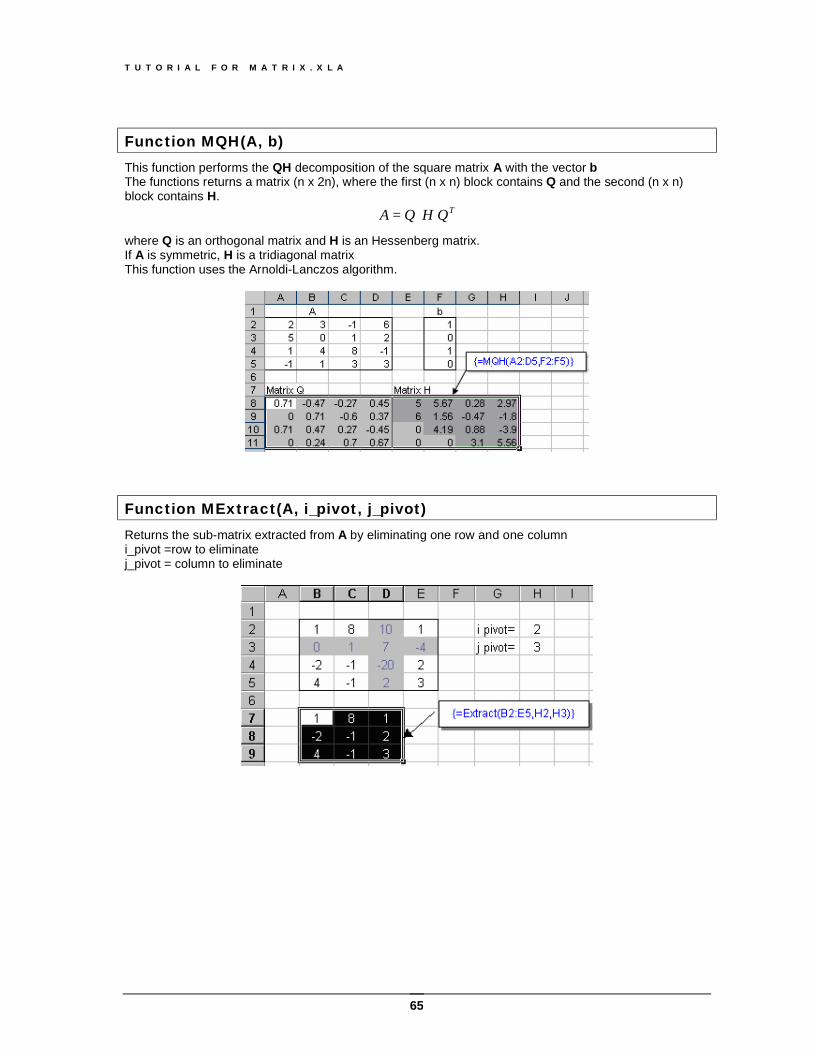
T U T O R I A L F O R M A T R I X . X L A
65
Function MQH(A, b) This function performs the QH decomposition of the square matrix A with the vector b The functions returns a matrix (n x 2n), where the first (n x n) block contains Q and the second (n x n) block contains H.
TQHQA =
where Q is an orthogonal matrix and H is an Hessenberg matrix. If A is symmetric, H is a tridiagonal matrix This function uses the Arnoldi-Lanczos algorithm.
Function MExtract(A, i_pivot, j_pivot) Returns the sub-matrix extracted from A by eliminating one row and one column i_pivot =row to eliminate j_pivot = column to eliminate
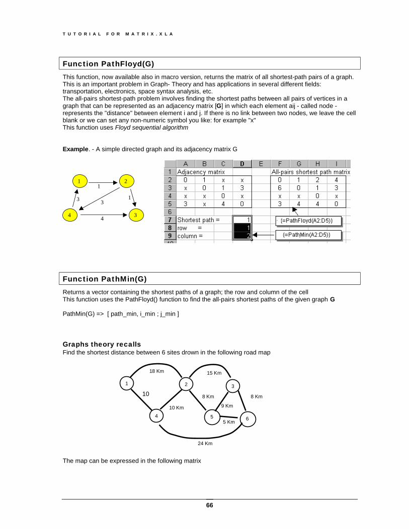
T U T O R I A L F O R M A T R I X . X L A
66
Function PathFloyd(G) This function, now available also in macro version, returns the matrix of all shortest-path pairs of a graph. This is an important problem in Graph- Theory and has applications in several different fields: transportation, electronics, space syntax analysis, etc. The all-pairs shortest-path problem involves finding the shortest paths between all pairs of vertices in a graph that can be represented as an adjacency matrix [G] in which each element aij - called node - represents the "distance" between element i and j. If there is no link between two nodes, we leave the cell blank or we can set any non-numeric symbol you like: for example "x" This function uses Floyd sequential algorithm Example. - A simple directed graph and its adjacency matrix G
1 2
4 3
1
13
4
3
Function PathMin(G) Returns a vector containing the shortest paths of a graph; the row and column of the cell This function uses the PathFloyd() function to find the all-pairs shortest paths of the given graph G PathMin(G) => [ path_min, i_min ; j_min ] Graphs theory recalls Find the shortest distance between 6 sites drown in the following road map The map can be expressed in the following matrix
1 2 3
4 5 6
18 Km
10
15 Km
10 Km
8 Km
5 Km
8 Km
9 Km
24 Km
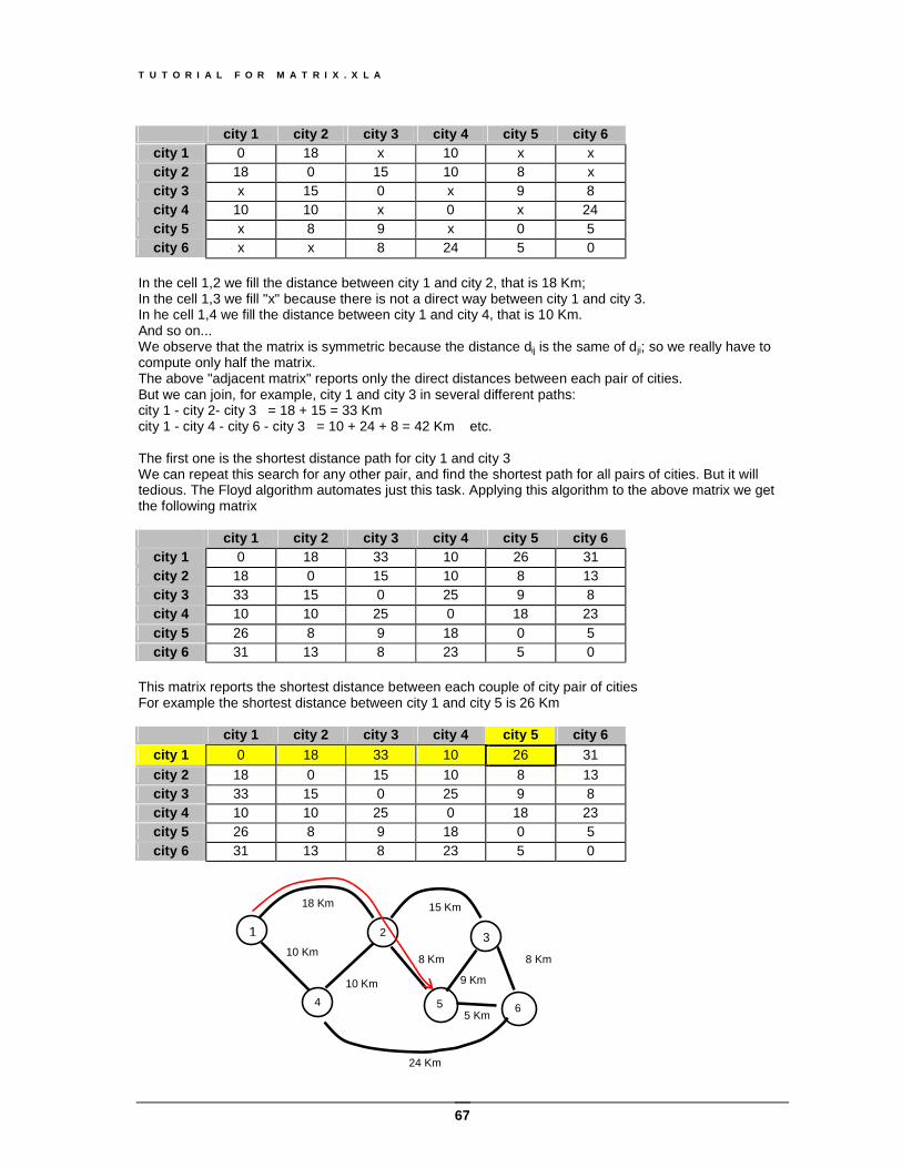
T U T O R I A L F O R M A T R I X . X L A
67
city 1 city 2 city 3 city 4 city 5 city 6 city 1 0 18 x 10 x x city 2 18 0 15 10 8 x city 3 x 15 0 x 9 8 city 4 10 10 x 0 x 24 city 5 x 8 9 x 0 5 city 6 x x 8 24 5 0
In the cell 1,2 we fill the distance between city 1 and city 2, that is 18 Km; In the cell 1,3 we fill "x" because there is not a direct way between city 1 and city 3. In he cell 1,4 we fill the distance between city 1 and city 4, that is 10 Km. And so on... We observe that the matrix is symmetric because the distance dij is the same of dji; so we really have to compute only half the matrix. The above "adjacent matrix" reports only the direct distances between each pair of cities. But we can join, for example, city 1 and city 3 in several different paths: city 1 - city 2- city 3 = 18 + 15 = 33 Km city 1 - city 4 - city 6 - city 3 = 10 + 24 + 8 = 42 Km etc. The first one is the shortest distance path for city 1 and city 3 We can repeat this search for any other pair, and find the shortest path for all pairs of cities. But it will tedious. The Floyd algorithm automates just this task. Applying this algorithm to the above matrix we get the following matrix
city 1 city 2 city 3 city 4 city 5 city 6 city 1 0 18 33 10 26 31 city 2 18 0 15 10 8 13 city 3 33 15 0 25 9 8 city 4 10 10 25 0 18 23 city 5 26 8 9 18 0 5 city 6 31 13 8 23 5 0
This matrix reports the shortest distance between each couple of city pair of cities For example the shortest distance between city 1 and city 5 is 26 Km
city 1 city 2 city 3 city 4 city 5 city 6 city 1 0 18 33 10 26 31 city 2 18 0 15 10 8 13 city 3 33 15 0 25 9 8 city 4 10 10 25 0 18 23 city 5 26 8 9 18 0 5 city 6 31 13 8 23 5 0
1 2 3
4 5 6
18 Km
10 Km
15 Km
10 Km
8 Km
5 Km
8 Km
9 Km
24 Km
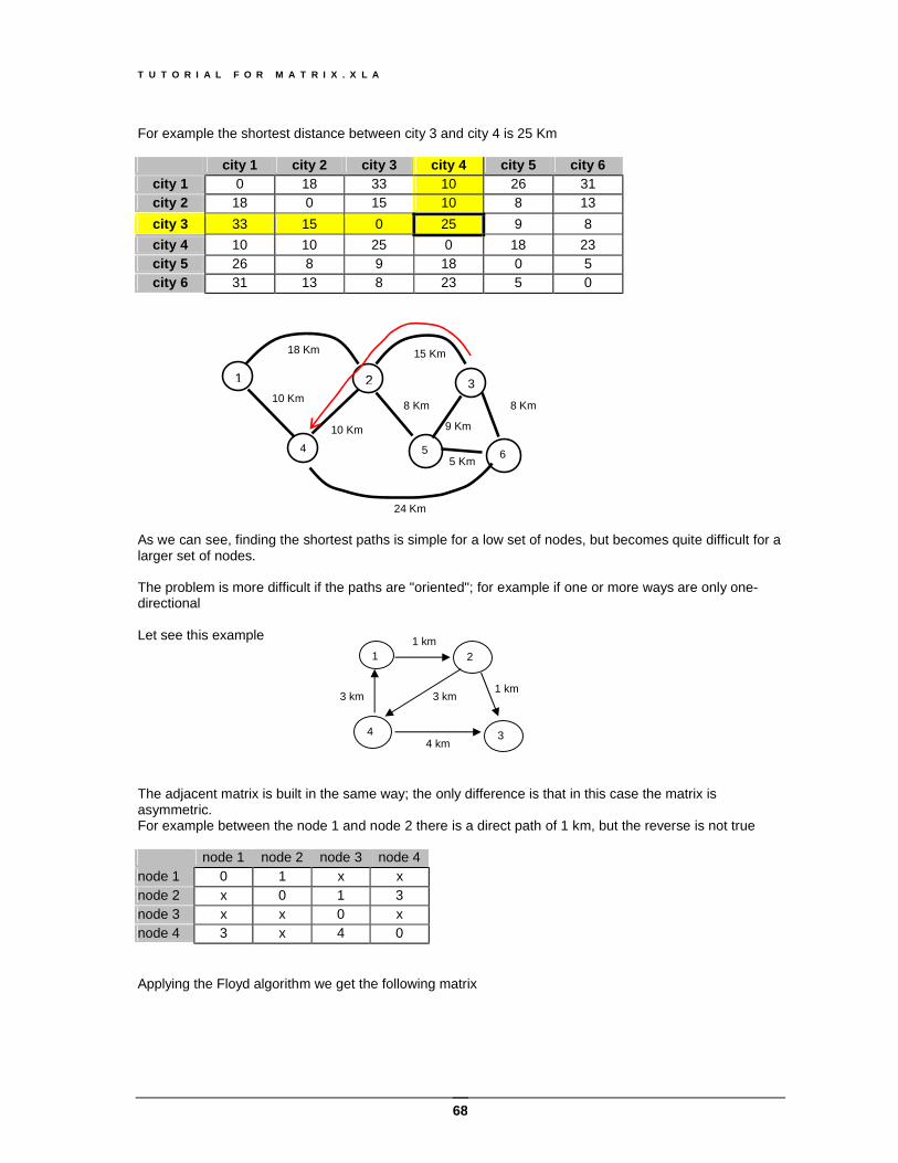
T U T O R I A L F O R M A T R I X . X L A
68
For example the shortest distance between city 3 and city 4 is 25 Km
city 1 city 2 city 3 city 4 city 5 city 6 city 1 0 18 33 10 26 31 city 2 18 0 15 10 8 13 city 3 33 15 0 25 9 8 city 4 10 10 25 0 18 23 city 5 26 8 9 18 0 5 city 6 31 13 8 23 5 0
As we can see, finding the shortest paths is simple for a low set of nodes, but becomes quite difficult for a larger set of nodes. The problem is more difficult if the paths are "oriented"; for example if one or more ways are only one-directional Let see this example The adjacent matrix is built in the same way; the only difference is that in this case the matrix is asymmetric. For example between the node 1 and node 2 there is a direct path of 1 km, but the reverse is not true
node 1 node 2 node 3 node 4 node 1 0 1 x x node 2 x 0 1 3 node 3 x x 0 x node 4 3 x 4 0 Applying the Floyd algorithm we get the following matrix
1 2 3
4 5 6
18 Km
10 Km
15 Km
10 Km
8 Km
5 Km
8 Km
9 Km
24 Km
1 2
4 3
1 km
3 km 1 km
3 km
4 km
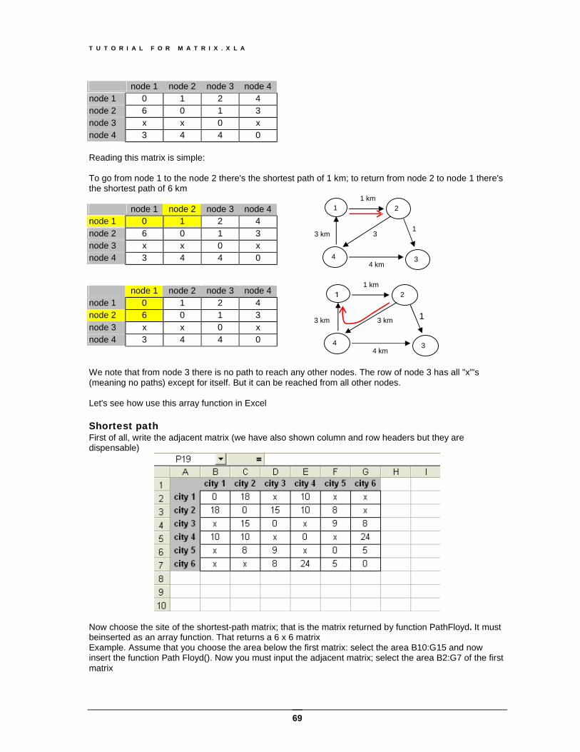
T U T O R I A L F O R M A T R I X . X L A
69
node 1 node 2 node 3 node 4 node 1 0 1 2 4 node 2 6 0 1 3 node 3 x x 0 x node 4 3 4 4 0 Reading this matrix is simple: To go from node 1 to the node 2 there's the shortest path of 1 km; to return from node 2 to node 1 there's the shortest path of 6 km
node 1 node 2 node 3 node 4 node 1 0 1 2 4 node 2 6 0 1 3 node 3 x x 0 x node 4 3 4 4 0
node 1 node 2 node 3 node 4 node 1 0 1 2 4 node 2 6 0 1 3 node 3 x x 0 x node 4 3 4 4 0 We note that from node 3 there is no path to reach any other nodes. The row of node 3 has all "x"'s (meaning no paths) except for itself. But it can be reached from all other nodes. Let's see how use this array function in Excel Shortest path First of all, write the adjacent matrix (we have also shown column and row headers but they are dispensable)
Now choose the site of the shortest-path matrix; that is the matrix returned by function PathFloyd. It must beinserted as an array function. That returns a 6 x 6 matrix Example. Assume that you choose the area below the first matrix: select the area B10:G15 and now insert the function Path Floyd(). Now you must input the adjacent matrix; select the area B2:G7 of the first matrix
1 2
4 3
1 km
3 km 1 k3
km
4 km
1 2
4 3
1 km
3 km 1 3 km
4 km
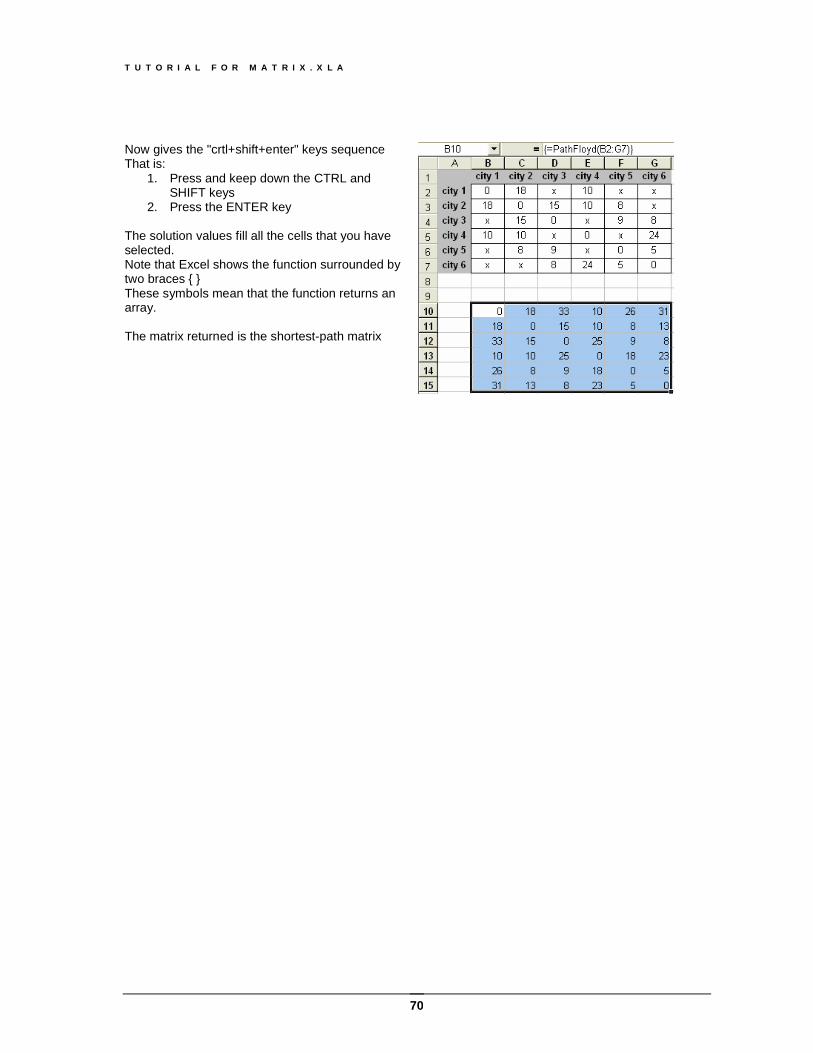
T U T O R I A L F O R M A T R I X . X L A
70
Now gives the "crtl+shift+enter" keys sequence That is:
1. Press and keep down the CTRL and SHIFT keys
2. Press the ENTER key The solution values fill all the cells that you have selected. Note that Excel shows the function surrounded by two braces { } These symbols mean that the function returns an array. The matrix returned is the shortest-path matrix
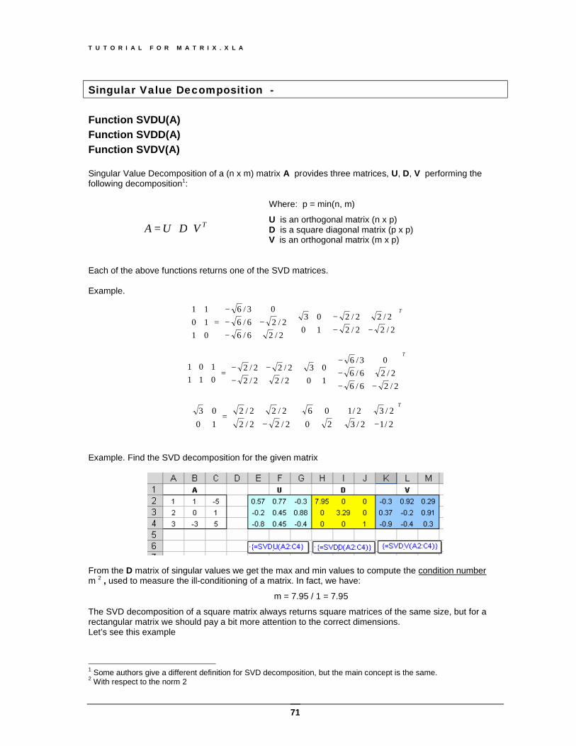
T U T O R I A L F O R M A T R I X . X L A
71
Singular Value Decomposition - Function SVDU(A) Function SVDD(A) Function SVDV(A) Singular Value Decomposition of a (n x m) matrix A provides three matrices, U, D, V performing the following decomposition1:
TVDUA ⋅⋅=
Where: p = min(n, m)
U is an orthogonal matrix (n x p) D is a square diagonal matrix (p x p) V is an orthogonal matrix (m x p)
Each of the above functions returns one of the SVD matrices. Example.
T
−−−
⋅
⋅
−−−
−=
2/22/22/22/2
1003
2/26/62/26/6
03/6
011011
T
−−−−
⋅
⋅
−−−
=
2/26/62/26/6
03/6
1003
2/22/22/22/2
011101
T
−⋅
⋅
−=
2/12/32/32/1
2006
2/22/22/22/2
1003
Example. Find the SVD decomposition for the given matrix
From the D matrix of singular values we get the max and min values to compute the condition number m 2 , used to measure the ill-conditioning of a matrix. In fact, we have:
m = 7.95 / 1 = 7.95
The SVD decomposition of a square matrix always returns square matrices of the same size, but for a rectangular matrix we should pay a bit more attention to the correct dimensions. Let’s see this example
1 Some authors give a different definition for SVD decomposition, but the main concept is the same. 2 With respect to the norm 2
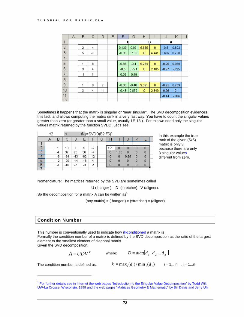
T U T O R I A L F O R M A T R I X . X L A
72
Sometimes it happens that the matrix is singular or “near singular”. The SVD decomposition evidences this fact, and allows computing the matrix rank in a very fast way. You have to count the singular values greater than zero (or greater than a small value, usually 1E-13 ). For this we need only the singular values matrix returned by the function SVDD. Let’s see.
Nomenclature: The matrices returned by the SVD are sometimes called
U ( hanger ), D (stretcher), V (aligner).
So the decomposition for a matrix A can be written as1
(any matrix) = ( hanger ) x (stretcher) x (aligner)
Condition Number This number is conventionally used to indicate how ill-conditioned a matrix is Formally the condition number of a matrix is defined by the SVD decomposition as the ratio of the largest element to the smallest element of diagonal matrix Given the SVD decomposition:
TUDVA = where: [ ] ... , 21 nddddiagD =
The condition number is defined as: )(min/)(max jjii dd=κ i = 1... n , j = 1...n
1 For further details see in Internet the web pages “Introduction to the Singular Value Decomposition” by Todd Will, UW-La Crosse, Wisconsin, 1999 and the web pages “Matrices Geometry & Mathematic” by Bill Davis and Jerry Uhl
In this example the true rank of the given (5x5) matrix is only 3, because there are only 3 singular values different from zero.
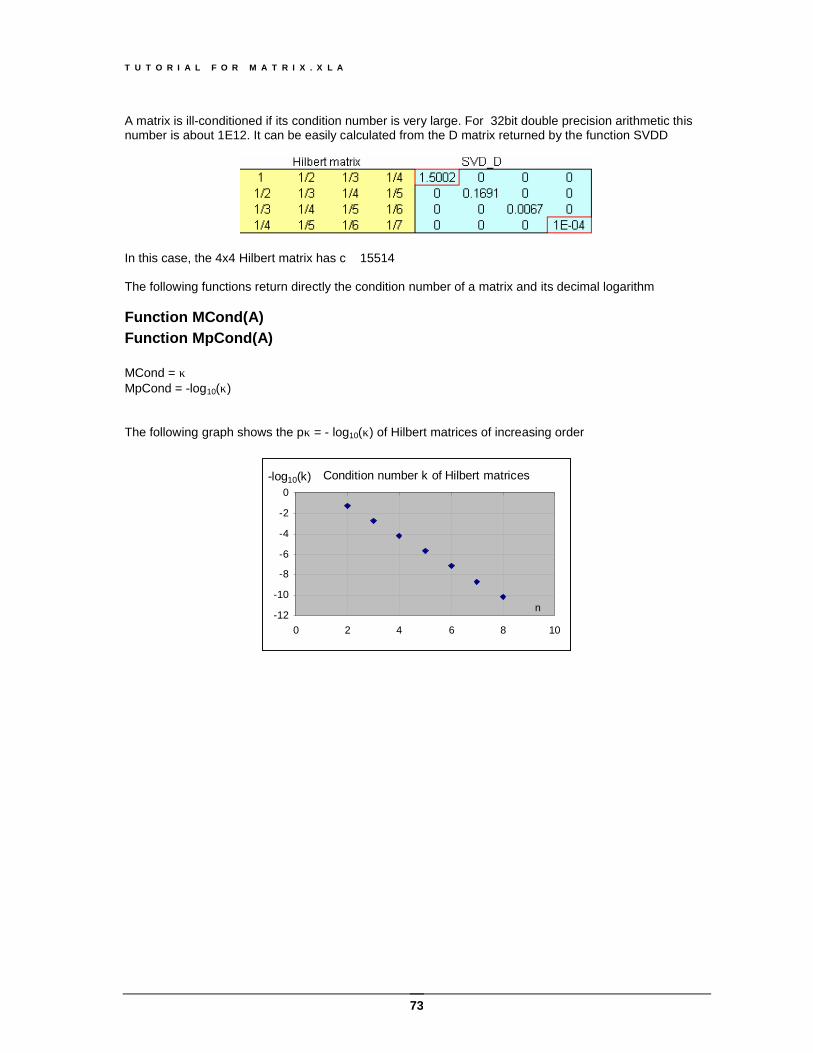
T U T O R I A L F O R M A T R I X . X L A
73
A matrix is ill-conditioned if its condition number is very large. For 32bit double precision arithmetic this number is about 1E12. It can be easily calculated from the D matrix returned by the function SVDD
In this case, the 4x4 Hilbert matrix has c ≅ 15514 The following functions return directly the condition number of a matrix and its decimal logarithm Function MCond(A) Function MpCond(A) MCond = κ MpCond = -log10(κ) The following graph shows the pκ = - log10(κ) of Hilbert matrices of increasing order
-12
-10
-8
-6
-4
-2
0
0 2 4 6 8 10
Condition number k of Hilbert matrices
n
-log10(k)
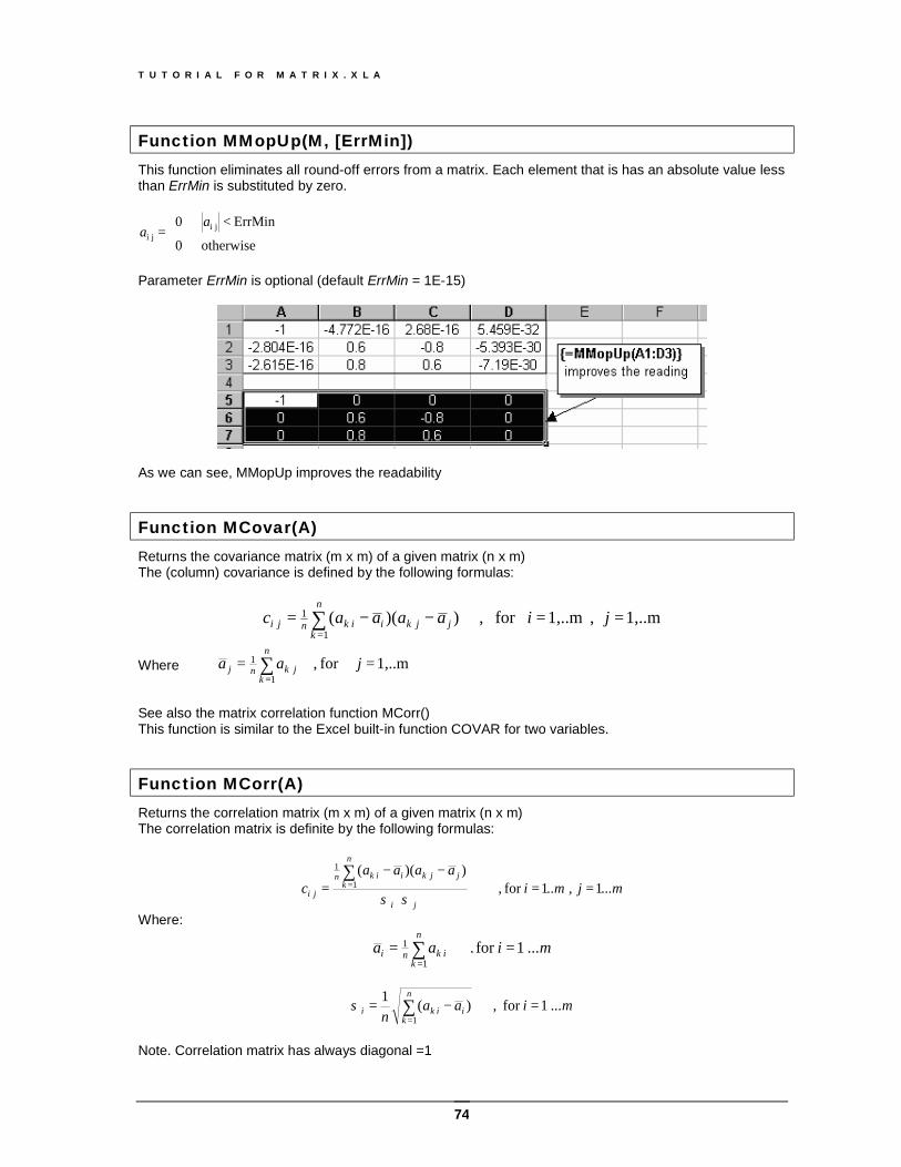
T U T O R I A L F O R M A T R I X . X L A
74
Function MMopUp(M, [ErrMin]) This function eliminates all round-off errors from a matrix. Each element that is has an absolute value less than ErrMin is substituted by zero.
⇒
<⇒=
otherwise0
ErrMin0 j ij i
aa
Parameter ErrMin is optional (default ErrMin = 1E-15)
As we can see, MMopUp improves the readability
Function MCovar(A) Returns the covariance matrix (m x m) of a given matrix (n x m) The (column) covariance is defined by the following formulas:
1,..m , 1,..mfor , ))(( 1
1
==−−= ∑=
jiaaaac jjk
n
kiiknji
Where See also the matrix correlation function MCorr() This function is similar to the Excel built-in function COVAR for two variables.
Function MCorr(A) Returns the correlation matrix (m x m) of a given matrix (n x m) The correlation matrix is definite by the following formulas:
...m j..m iaaaa
cji
n
kjjkiikn
ji 1,1for , ))((
1
1
==⋅
−−=
∑=
σσ Where:
...miaan
kikni 1for .
1
1 == ∑=
...miaan
n
kiiki 1for , )(1
1 =−= ∑
=σ
Note. Correlation matrix has always diagonal =1
1,..mfor , 1
1 == ∑
=jaa
n
kjknj
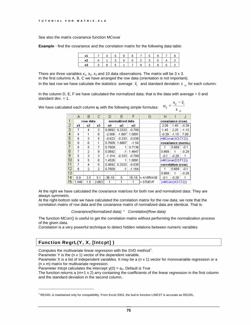
T U T O R I A L F O R M A T R I X . X L A
75
See also the matrix covariance function MCovar Example - find the covariance and the correlation matrix for the following data table:
x1 7 4 6 8 8 7 5 9 7 8 x2 4 1 3 6 5 2 3 5 4 2 x3 3 8 5 1 7 9 3 8 5 2
There are three variables x1, x2, x3 and 10 data observations. The matrix will be 3 x 3. In the first columns A, B, C we have arranged the row data (orientation is not important). In the last row we have calculate the statistics: average ix and standard deviation xiσ for each column. In the column D, E, F we have calculated the normalized data; that is the data with average = 0 and standard dev. = 1. We have calculated each column ui with the following simple formulas:
At the right we have calculated the covariance matrices for both row and normalized data: They are always symmetric. At the right-bottom side we have calculated the correlation matrix for the row data; we note that the correlation matrix of row data and the covariance matrix of normalized data are identical. That is:
Covariance(Normalized data) ≡ Correlation(Row data)
The function MCorr() is useful to get the correlation matrix without performing the normalization process of the given data. Correlation is a very powerful technique to detect hidden relations between numeric variables
Function RegrL(Y, X, [Intcpt] ) Computes the multivariate linear regression with the SVD method1. Parameter Y is the (n x 1) vector of the dependent variable. Parameter X is a list of independent variables. It may be a (n x 1) vector for monovariable regression or a (n x m) matrix for multivariate regression. Parameter Intcpt calculates the intercept y(0) = a0. Default is True The function returns a (m+1 x 2) arry containing the coefficients of the linear regression in the first column and the standard deviation in the second column..
1 REGRL is maintained only for compatibility. From Excel 2003, the buil-in function LINEST is accurate as REGRL.
xi
iijij
xxu
σ−
=
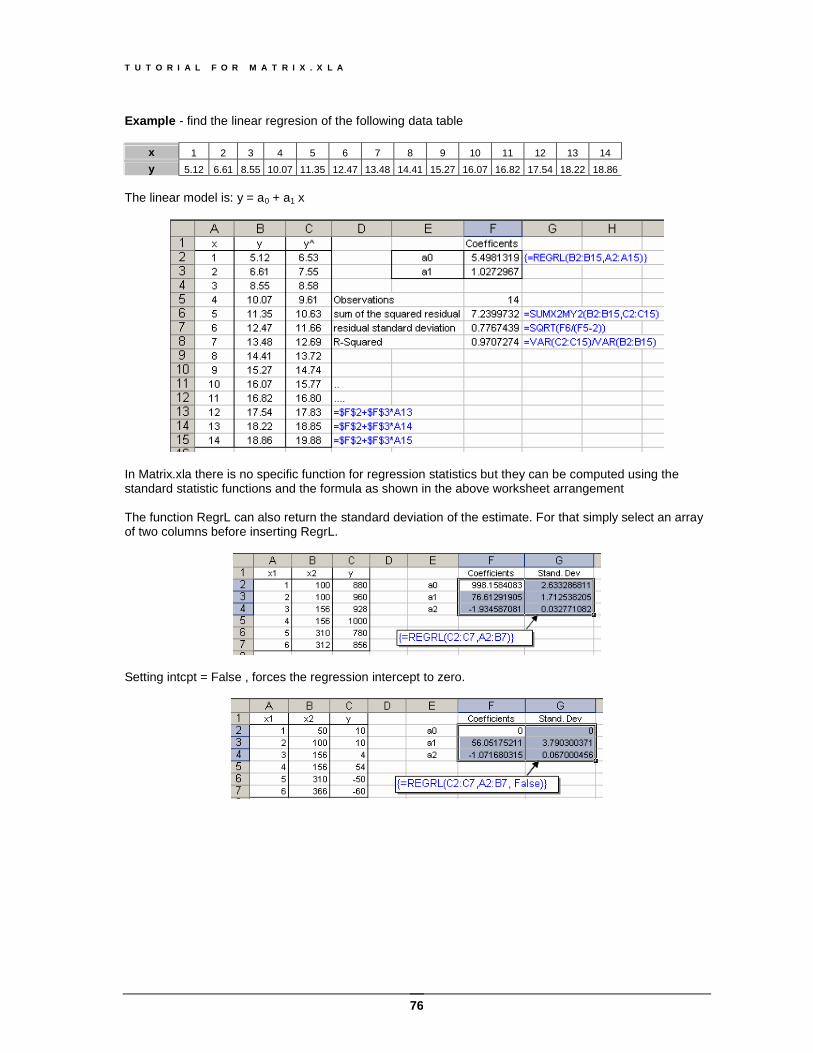
T U T O R I A L F O R M A T R I X . X L A
76
Example - find the linear regresion of the following data table
x 1 2 3 4 5 6 7 8 9 10 11 12 13 14 y 5.12 6.61 8.55 10.07 11.35 12.47 13.48 14.41 15.27 16.07 16.82 17.54 18.22 18.86
The linear model is: y = a0 + a1 x
In Matrix.xla there is no specific function for regression statistics but they can be computed using the standard statistic functions and the formula as shown in the above worksheet arrangement The function RegrL can also return the standard deviation of the estimate. For that simply select an array of two columns before inserting RegrL.
Setting intcpt = False , forces the regression intercept to zero.
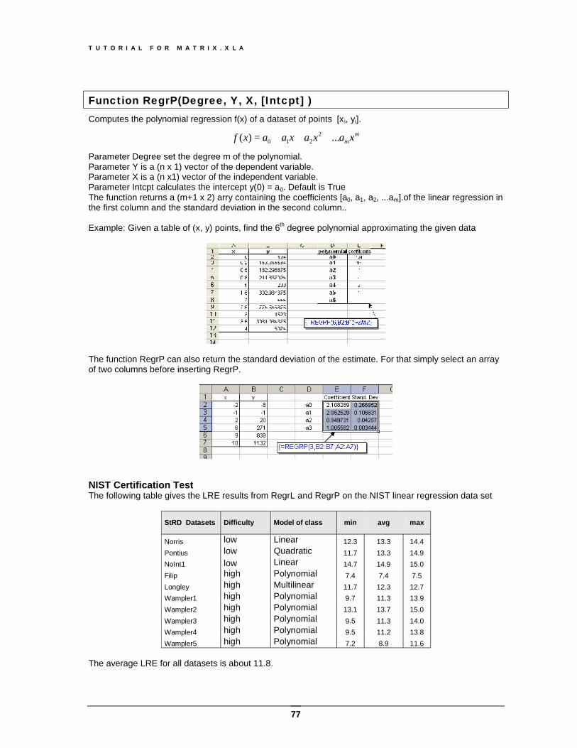
T U T O R I A L F O R M A T R I X . X L A
77
Function RegrP(Degree, Y, X, [Intcpt] ) Computes the polynomial regression f(x) of a dataset of points [x i, yi].
mmxaxaxaaxf ...)( 2
210 +++= Parameter Degree set the degree m of the polynomial. Parameter Y is a (n x 1) vector of the dependent variable. Parameter X is a (n x1) vector of the independent variable. Parameter Intcpt calculates the intercept y(0) = a0. Default is True The function returns a (m+1 x 2) arry containing the coefficients [a0, a1, a2, ...am].of the linear regression in the first column and the standard deviation in the second column.. Example: Given a table of (x, y) points, find the 6th degree polynomial approximating the given data
The function RegrP can also return the standard deviation of the estimate. For that simply select an array of two columns before inserting RegrP.
NIST Certification Test The following table gives the LRE results from RegrL and RegrP on the NIST linear regression data set
StRD Datasets Difficulty Model of class min avg max
Norris low Linear 12.3 13.3 14.4 Pontius low Quadratic 11.7 13.3 14.9 NoInt1 low Linear 14.7 14.9 15.0 Filip high Polynomial 7.4 7.4 7.5 Longley high Multilinear 11.7 12.3 12.7 Wampler1 high Polynomial 9.7 11.3 13.9 Wampler2 high Polynomial 13.1 13.7 15.0 Wampler3 high Polynomial 9.5 11.3 14.0 Wampler4 high Polynomial 9.5 11.2 13.8 Wampler5 high Polynomial 7.2 8.9 11.6
The average LRE for all datasets is about 11.8.
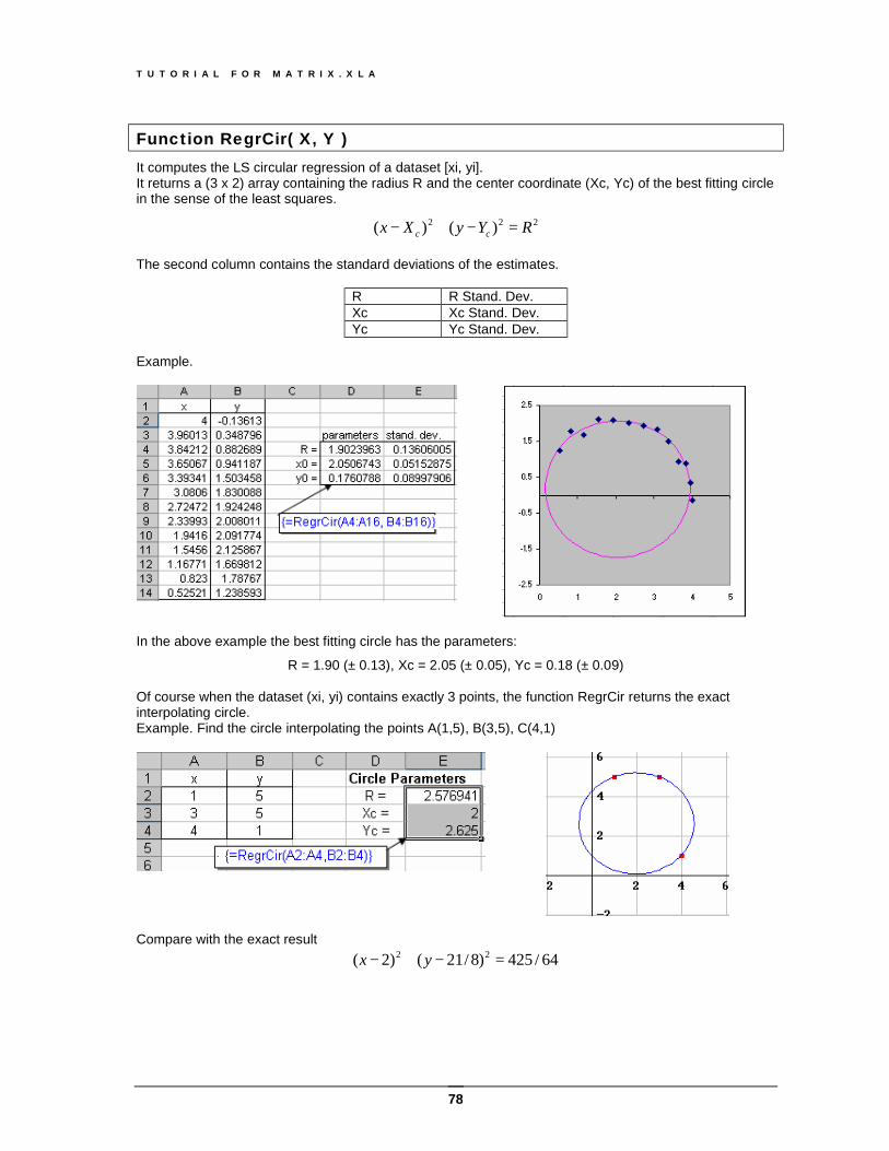
T U T O R I A L F O R M A T R I X . X L A
78
Function RegrCir( X, Y ) It computes the LS circular regression of a dataset [xi, yi]. It returns a (3 x 2) array containing the radius R and the center coordinate (Xc, Yc) of the best fitting circle in the sense of the least squares.
222 )()( RYyXx cc =−+− The second column contains the standard deviations of the estimates.
R R Stand. Dev. Xc Xc Stand. Dev. Yc Yc Stand. Dev.
Example.
In the above example the best fitting circle has the parameters:
R = 1.90 (± 0.13), Xc = 2.05 (± 0.05), Yc = 0.18 (± 0.09) Of course when the dataset (xi, yi) contains exactly 3 points, the function RegrCir returns the exact interpolating circle. Example. Find the circle interpolating the points A(1,5), B(3,5), C(4,1)
Compare with the exact result
64/425)8/21()2( 22 =−+− yx
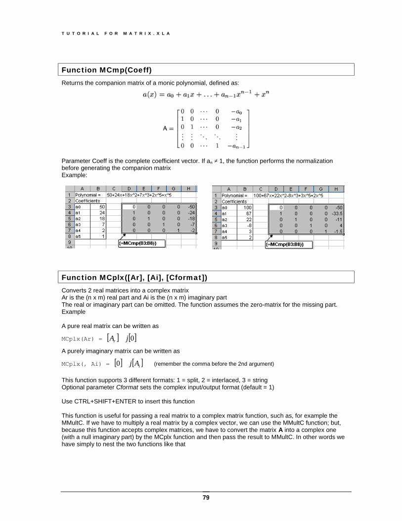
T U T O R I A L F O R M A T R I X . X L A
79
Function MCmp(Coeff) Returns the companion matrix of a monic polynomial, defined as:
Parameter Coeff is the complete coefficient vector. If an ≠ 1, the function performs the normalization before generating the companion matrix Example:
Function MCplx([Ar], [Ai], [Cformat]) Converts 2 real matrices into a complex matrix Ar is the (n x m) real part and Ai is the (n x m) imaginary part The real or imaginary part can be omitted. The function assumes the zero-matrix for the missing part. Example A pure real matrix can be written as
MCplx(Ar) = [ ] [ ]0jAr + A purely imaginary matrix can be written as
MCplx(, Ai) = [ ] [ ]iAj+0 (remember the comma before the 2nd argument)
This function supports 3 different formats: 1 = split, 2 = interlaced, 3 = string Optional parameter Cformat sets the complex input/output format (default = 1) Use CTRL+SHIFT+ENTER to insert this function This function is useful for passing a real matrix to a complex matrix function, such as, for example the MMultC. If we have to multiply a real matrix by a complex vector, we can use the MMultC function; but, because this function accepts complex matrices, we have to convert the matrix A into a complex one (with a null imaginary part) by the MCplx function and then pass the result to MMultC. In other words we have simply to nest the two functions like that
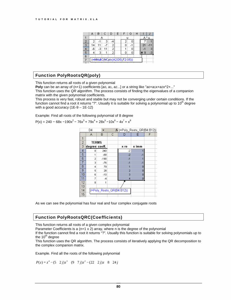
T U T O R I A L F O R M A T R I X . X L A
80
Function PolyRootsQR(poly) This function returns all roots of a given polynomial Poly can be an array of (n+1) coefficients [a0, a1, a2...] or a string like "a0+a1x+a2x^2+..." This function uses the QR algorithm. The process consists of finding the eigenvalues of a companion matrix with the given polynomial coefficients. This process is very fast, robust and stable but may not be converging under certain conditions. If the function cannot find a root it returns “?”. Usually it is suitable for solving a polynomial up to 10th degree with a good accuracy (1E-9 – 1E-12) Example: Find all roots of the following polynomial of 8 degree
P(x) = 240 − 68x −190x2 − 76x3 + 79x4 + 28x5 −10x6 − 4x7 + x8
As we can see the polynomial has four real and four complex conjugate roots
Function PolyRootsQRC(Coefficients) This function returns all roots of a given complex polynomial Parameter Coefficients is a (n+1 x 2) array, where n is the degree of the polynomial If the function cannot find a root it returns “?”. Usually this function is suitable for solving polynomials up to the 10th degree This function uses the QR algorithm. The process consists of iteratively applying the QR decomposition to the complex companion matrix. Example. Find all the roots of the following polynomial
jzjzjzjzzP 248)222()79()25()( 234 +++−+++−=
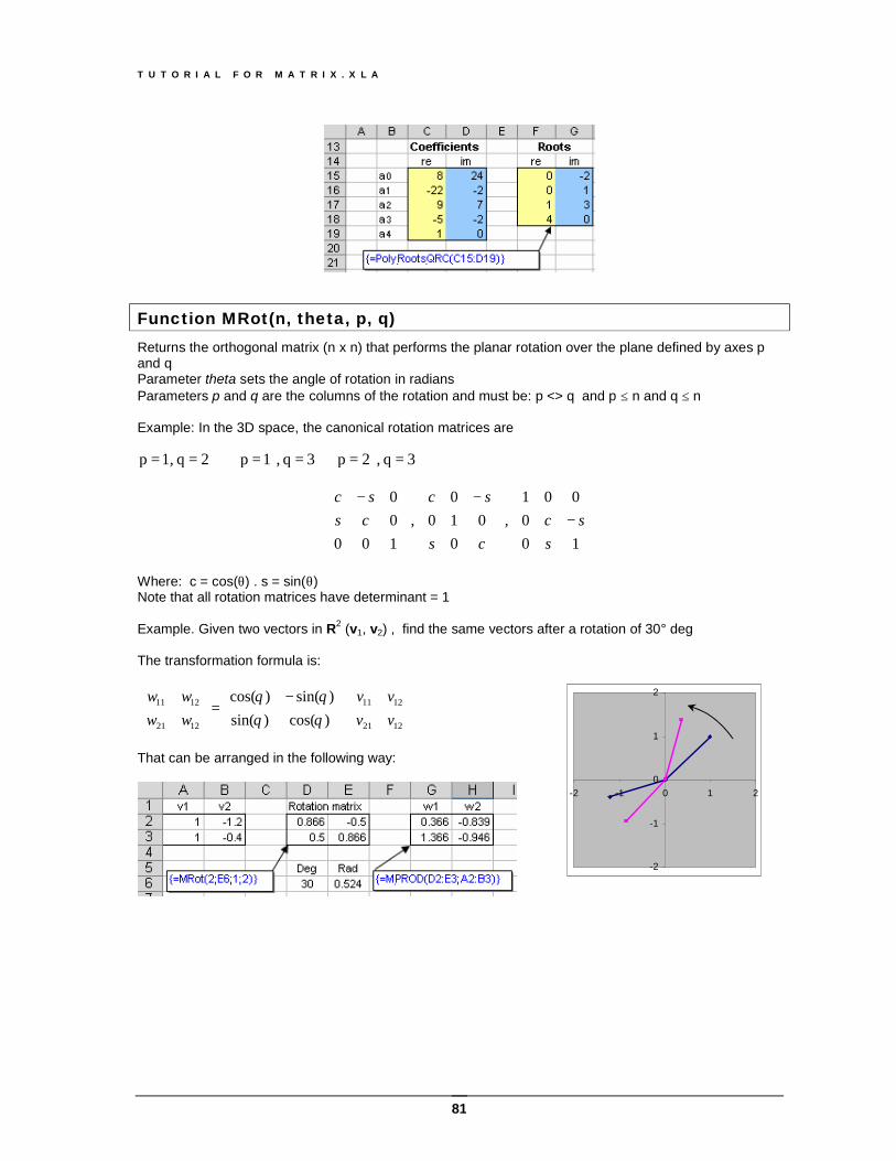
T U T O R I A L F O R M A T R I X . X L A
81
Function MRot(n, theta, p, q) Returns the orthogonal matrix (n x n) that performs the planar rotation over the plane defined by axes p and q Parameter theta sets the angle of rotation in radians Parameters p and q are the columns of the rotation and must be: p <> q and p ≤ n and q ≤ n Example: In the 3D space, the canonical rotation matrices are
3q , 2p 3q , 1p 2q 1,p ======
−
−
−
100
001 ,
0010
0 ,
10000
ssc
cs
sccssc
Where: c = cos(θ) . s = sin(θ) Note that all rotation matrices have determinant = 1 Example. Given two vectors in R2 (v1, v2) , find the same vectors after a rotation of 30° deg The transformation formula is:
⋅
−=
1221
1211
1221
1211
)cos()sin()sin()cos(
vvvv
wwww
θθθθ
That can be arranged in the following way:
-2
-1
0
1
2
-2 -1 0 1 2
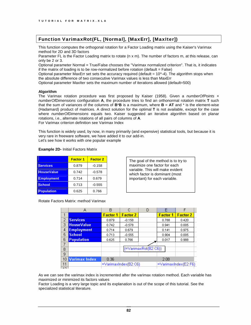
T U T O R I A L F O R M A T R I X . X L A
82
Function VarimaxRot(FL, [Normal], [MaxErr], [MaxIter]) This function computes the orthogonal rotation for a Factor Loading matrix using the Kaiser's Varimax method for 2D and 3D factors Parameter FL is the Factor Loading matrix to rotate (n x m). The number of factors m, at this release, can only be 2 or 3. Optional parameter Normal = True/False chooses the "Varimax normalized criterion". That is, it indicates if the matrix of loading is to be row-normalized before rotation (default = False) Optional parameter MaxErr set sets the accuracy required (default = 10^-4). The algorithm stops when the absolute difference of two consecutive Varimax values is less than MaxErr Optional parameter MaxIter sets the maximum number of iterations allowed (default=500) Algorithm The Varimax rotation procedure was first proposed by Kaiser (1958). Given a numberOfPoints × numberOfDimensions configuration A, the procedure tries to find an orthonormal rotation matrix T such that the sum of variances of the columns of B*B is a maximum, where B = AT and * is the element-wise (Hadamard) product of matrices. A direct solution for the optimal T is not available, except for the case where numberOfDimensions equals two. Kaiser suggested an iterative algorithm based on planar rotations, i.e., alternate rotations of all pairs of columns of A. For Varimax criterion definition see Varimax Index This function is widely used, by now, in many primarily (and expensive) statistical tools, but because it is very rare in freeware software, we have added it to our add-in. Let's see how it works with one popular example Example 2D- Initial Factors Matrix Factor 1 Factor 2
Services 0.879 -0.158
HouseValue 0.742 -0.578
Employment 0.714 0.679
School 0.713 -0.555
Population 0.625 0.766 Rotate Factors Matrix: method Varimax
As we can see the varimax index is incremented after the varimax rotation method. Each variable has maximized or minimized its factors values Factor Loading is a very large topic and its explanation is out of the scope of this tutorial. See the specialized statistical literature.
The goal of the method is to try to maximize one factor for each variable. This will make evident which factor is dominant (most important) for each variable.
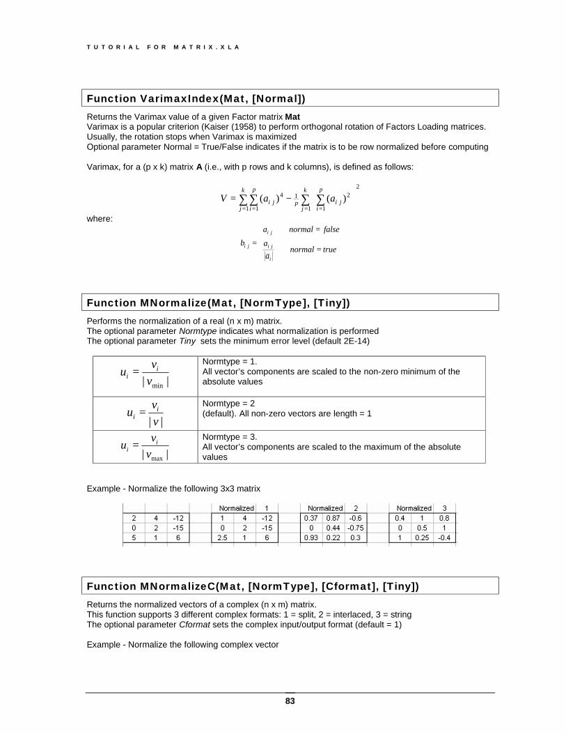
T U T O R I A L F O R M A T R I X . X L A
83
Function VarimaxIndex(Mat, [Normal]) Returns the Varimax value of a given Factor matrix Mat Varimax is a popular criterion (Kaiser (1958) to perform orthogonal rotation of Factors Loading matrices. Usually, the rotation stops when Varimax is maximized Optional parameter Normal = True/False indicates if the matrix is to be row normalized before computing Varimax, for a (p x k) matrix A (i.e., with p rows and k columns), is defined as follows:
2
1
2
1
14
1 1 )()( ∑ ∑∑∑
= == =
−=
k
j
p
ijip
k
j
p
iji aaV
where:
=⇒
=⇒
=truenormal
aa
falsenormalab
i
ji
ji
ji
Function MNormalize(Mat, [NormType], [Tiny]) Performs the normalization of a real (n x m) matrix. The optional parameter Normtype indicates what normalization is performed The optional parameter Tiny sets the minimum error level (default 2E-14)
|| minvvu i
i =
Normtype = 1. All vector’s components are scaled to the non-zero minimum of the absolute values
|| vvu i
i =
Normtype = 2 (default). All non-zero vectors are length = 1
|| maxvvu i
i =
Normtype = 3. All vector’s components are scaled to the maximum of the absolute values
Example - Normalize the following 3x3 matrix
Function MNormalizeC(Mat, [NormType], [Cformat], [Tiny]) Returns the normalized vectors of a complex (n x m) matrix. This function supports 3 different complex formats: 1 = split, 2 = interlaced, 3 = string The optional parameter Cformat sets the complex input/output format (default = 1) Example - Normalize the following complex vector
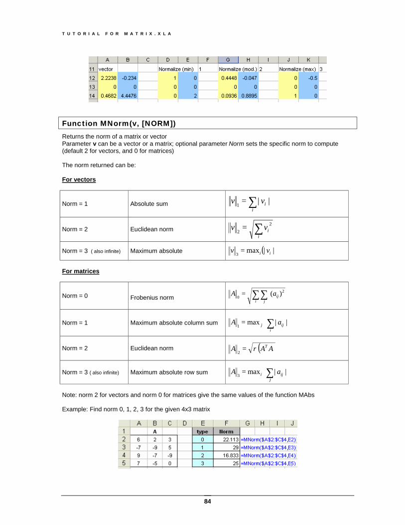
T U T O R I A L F O R M A T R I X . X L A
84
Function MNorm(v, [NORM]) Returns the norm of a matrix or vector Parameter v can be a vector or a matrix; optional parameter Norm sets the specific norm to compute (default 2 for vectors, and 0 for matrices) The norm returned can be: For vectors
Norm = 1 Absolute sum ∑=i
ivv ||1
Norm = 2 Euclidean norm ∑=i
ivv 22
Norm = 3 ( also infinite) Maximum absolute ( )||max3 ii vv =
For matrices
Norm = 0 Frobenius norm ∑∑=i j
ijaA 20
)(
Norm = 1 Maximum absolute column sum
= ∑
iijj aA ||max
1
Norm = 2 Euclidean norm ( )AAA Tρ=2
Norm = 3 ( also infinite) Maximum absolute row sum
= ∑
jiji aA ||max
3
Note: norm 2 for vectors and norm 0 for matrices give the same values of the function MAbs Example: Find norm 0, 1, 2, 3 for the given 4x3 matrix
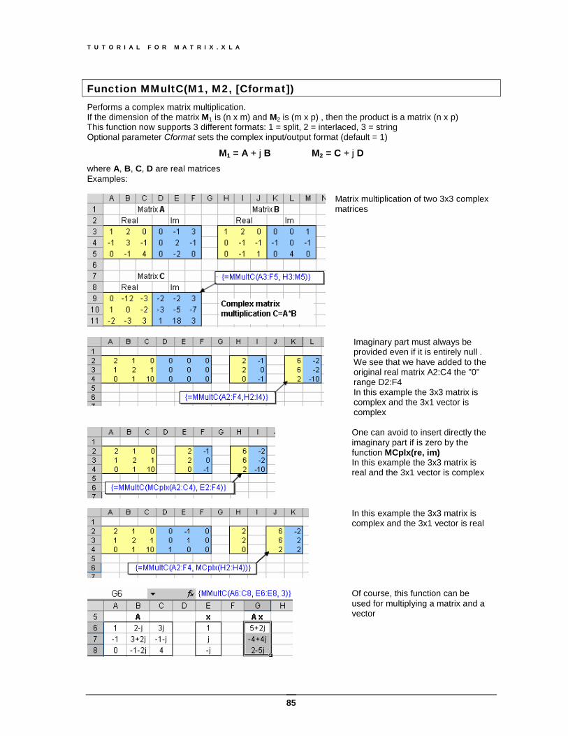
T U T O R I A L F O R M A T R I X . X L A
85
Function MMultC(M1, M2, [Cformat]) Performs a complex matrix multiplication. If the dimension of the matrix M1 is (n x m) and M2 is (m x p) , then the product is a matrix (n x p) This function now supports 3 different formats: 1 = split, 2 = interlaced, 3 = string Optional parameter Cformat sets the complex input/output format (default = 1)
M1 = A + j B M2 = C + j D where A, B, C, D are real matrices Examples:
Matrix multiplication of two 3x3 complex matrices
Imaginary part must always be provided even if it is entirely null . We see that we have added to the original real matrix A2:C4 the "0" range D2:F4 In this example the 3x3 matrix is complex and the 3x1 vector is complex
One can avoid to insert directly the imaginary part if is zero by the function MCplx(re, im) In this example the 3x3 matrix is real and the 3x1 vector is complex
In this example the 3x3 matrix is complex and the 3x1 vector is real
Of course, this function can be used for multiplying a matrix and a vector
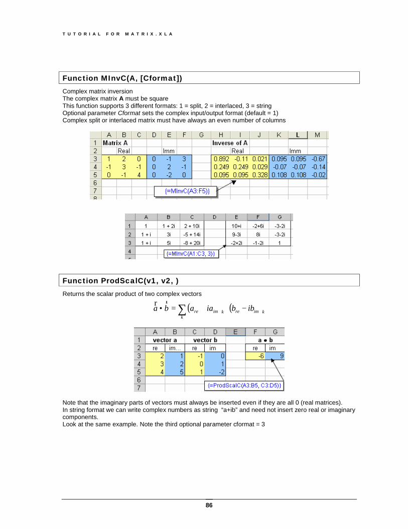
T U T O R I A L F O R M A T R I X . X L A
86
Function MInvC(A, [Cformat]) Complex matrix inversion The complex matrix A must be square This function supports 3 different formats: 1 = split, 2 = interlaced, 3 = string Optional parameter Cformat sets the complex input/output format (default = 1) Complex split or interlaced matrix must have always an even number of columns
Function ProdScalC(v1, v2, ) Returns the scalar product of two complex vectors
( ) ( )kimrek
kimre ibbiaaba −⋅+=• ∑rr
Note that the imaginary parts of vectors must always be inserted even if they are all 0 (real matrices). In string format we can write complex numbers as string “a+ib” and need not insert zero real or imaginary components. Look at the same example. Note the third optional parameter cformat = 3
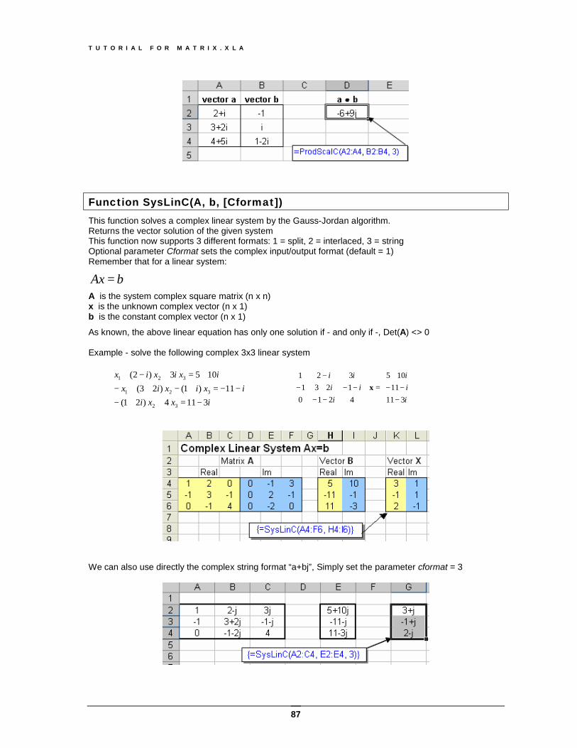
T U T O R I A L F O R M A T R I X . X L A
87
Function SysLinC(A, b, [Cformat]) This function solves a complex linear system by the Gauss-Jordan algorithm. Returns the vector solution of the given system This function now supports 3 different formats: 1 = split, 2 = interlaced, 3 = string Optional parameter Cformat sets the complex input/output format (default = 1) Remember that for a linear system:
bAx = A is the system complex square matrix (n x n) x is the unknown complex vector (n x 1) b is the constant complex vector (n x 1)
As known, the above linear equation has only one solution if - and only if -, Det(A) <> 0 Example - solve the following complex 3x3 linear system
−=++−−−=+−++−
+=+−+
ixxiixixix
ixixix
311 4 )21(11 )1( )23(
105 3 )2(
32
321
321
We can also use directly the complex string format “a+bj”, Simply set the parameter cformat = 3
−−−
+=⋅
−−−−+−
−
iii
iii
ii
31111
105
42101231321
x
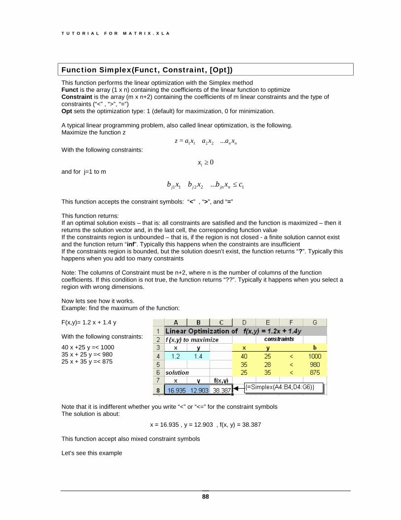
T U T O R I A L F O R M A T R I X . X L A
88
Function Simplex(Funct, Constraint, [Opt]) This function performs the linear optimization with the Simplex method Funct is the array (1 x n) containing the coefficients of the linear function to optimize Constraint is the array (m x n+2) containing the coefficients of m linear constraints and the type of constraints (“<” , “>”, “=”) Opt sets the optimization type: 1 (default) for maximization, 0 for minimization. A typical linear programming problem, also called linear optimization, is the following. Maximize the function z
nn xaxaxaz ...2211 ++= With the following constraints:
0≥ix and for j=1 to m
12211 ... cxbxbxb njnjj ≤++
This function accepts the constraint symbols: “<” , “>”, and “=” This function returns: If an optimal solution exists – that is: all constraints are satisfied and the function is maximized – then it returns the solution vector and, in the last cell, the corresponding function value If the constraints region is unbounded – that is, if the region is not closed - a finite solution cannot exist and the function return “inf”. Typically this happens when the constraints are insufficient If the constraints region is bounded, but the solution doesn’t exist, the function returns “?”. Typically this happens when you add too many constraints Note: The columns of Constraint must be n+2, where n is the number of columns of the function coefficients. If this condition is not true, the function returns “??”. Typically it happens when you select a region with wrong dimensions. Now lets see how it works. Example: find the maximum of the function: F(x,y)= 1.2 x + 1.4 y With the following constraints:
40 x +25 y =< 1000 35 x + 25 y =< 980 25 x + 35 y =< 875
Note that it is indifferent whether you write “<” or “<=” for the constraint symbols The solution is about:
x = 16.935 , y = 12.903 , f(x, y) = 38.387 This function accept also mixed constraint symbols Let’s see this example
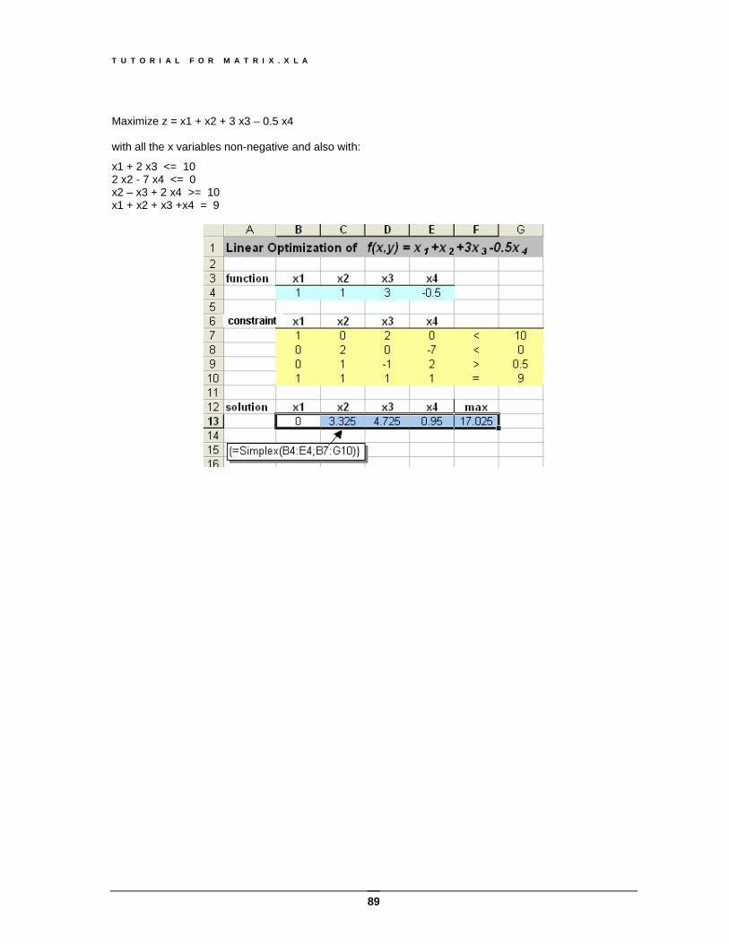
T U T O R I A L F O R M A T R I X . X L A
89
Maximize z = x1 + x2 + 3 x3 – 0.5 x4 with all the x variables non-negative and also with:
x1 + 2 x3 <= 10 2 x2 - 7 x4 <= 0 x2 – x3 + 2 x4 >= 10 x1 + x2 + x3 +x4 = 9
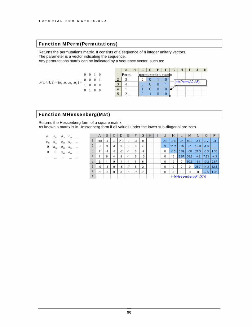
T U T O R I A L F O R M A T R I X . X L A
90
Function MPerm(Permutations) Returns the permutations matrix. It consists of a sequence of n integer unitary vectors. The parameter is a vector indicating the sequence. Any permutations matrix can be indicated by a sequence vector, such as:
==
0010000110000100
) , , , ()2 ,1 ,4 ,3( 2143 uuuuP
Function MHessenberg(Mat) Returns the Hessenberg form of a square matrix As known a matrix is in Hessenberg form if all values under the lower sub-diagonal are zero.
...............
...00
...0
...
...
4443
343332
24232221
14131211
aaaaaaaaaaaaa
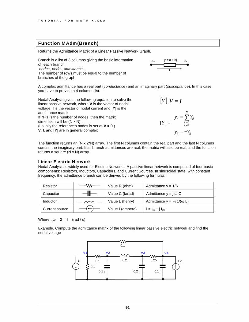
T U T O R I A L F O R M A T R I X . X L A
91
Function MAdm(Branch) Returns the Admittance Matrix of a Linear Passive Network Graph. Branch is a list of 3 columns giving the basic information of each branch: node+, node-, admittance . The number of rows must be equal to the number of branches of the graph
n-n+ y = a + bj
I
A complex admittance has a real part (conductance) and an imaginary part (susceptance). In this case you have to provide a 4 columns list. Nodal Analysis gives the following equation to solve the linear passive network, where V is the vector of nodal voltage, I is the vector of nodal current and [Y] is the admittance matrix. If N+1 is the number of nodes, then the matrix dimension will be (N x N). (usually the references nodes is set at V = 0 ) V, I, and [Y] are in general complex
[ ] IVY =⋅
−=
==
∑≠=
ijij
N
ikk
ikii
Yy
YyY 0][
The function returns an (N x 2*N) array. The first N columns contain the real part and the last N columns contain the imaginary part. If all branch-admittances are real, the matrix will also be real, and the function returns a square (N x N) array. Linear Electric Network Nodal Analysis is widely used for Electric Networks. A passive linear network is composed of four basic components: Resistors, Inductors, Capacitors, and Current Sources. In sinusoidal state, with constant frequency, the admittance branch can be derived by the following formulas
Resistor Value R (ohm) Admittance y = 1/R
Capacitor Value C (farad) Admittance y = j ω C
Inductor Value L (henry) Admittance y = −j 1/(ω L)
Current source Value I (ampere) I = Ire + j Iim
Where : ω = 2 π f (rad / s) Example. Compute the admittance matrix of the following linear passive electric network and find the nodal voltage
0.1 j 0.2 j 0.1 j
−0.2 j0.1 0.25
0.1
0.1
1.21
V1 V2 V3 V4
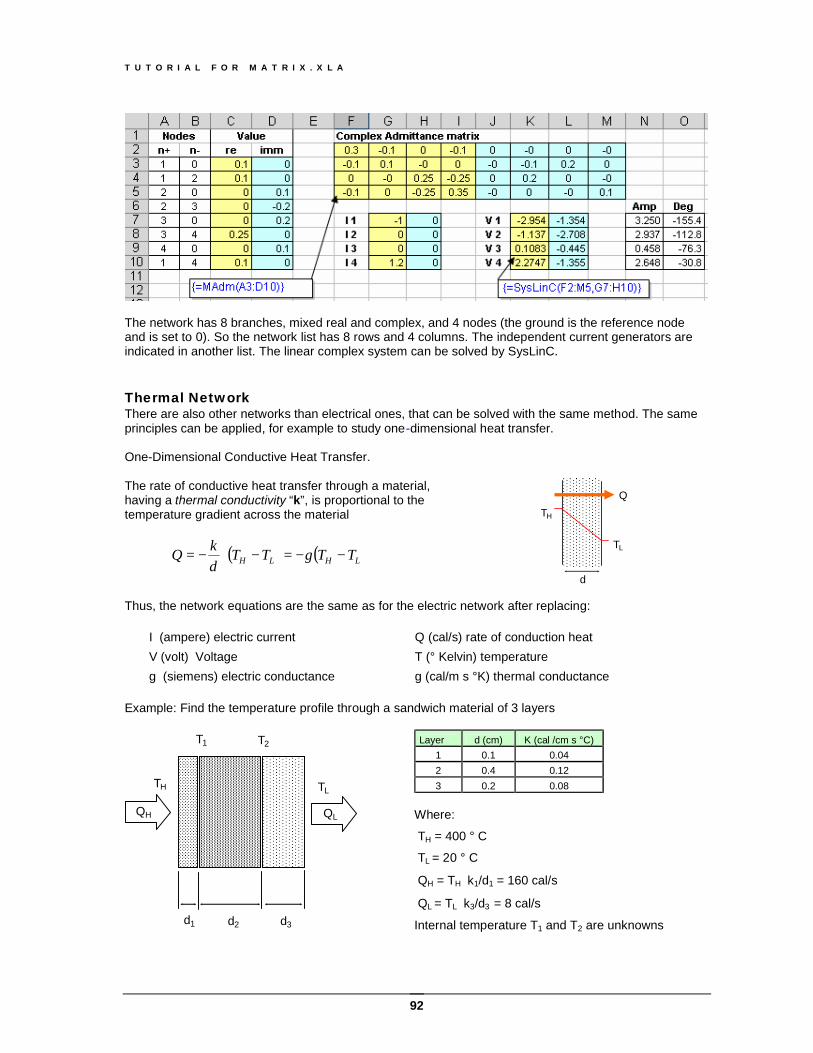
T U T O R I A L F O R M A T R I X . X L A
92
The network has 8 branches, mixed real and complex, and 4 nodes (the ground is the reference node and is set to 0). So the network list has 8 rows and 4 columns. The independent current generators are indicated in another list. The linear complex system can be solved by SysLinC. Thermal Network There are also other networks than electrical ones, that can be solved with the same method. The same principles can be applied, for example to study one-dimensional heat transfer. One-Dimensional Conductive Heat Transfer. The rate of conductive heat transfer through a material, having a thermal conductivity “k”, is proportional to the temperature gradient across the material
( ) ( )LHLH TTgTT
dkQ −−=−⋅−=
TH
TL
d
Q
Thus, the network equations are the same as for the electric network after replacing:
I (ampere) electric current ⇔ Q (cal/s) rate of conduction heat V (volt) Voltage ⇔ T (° Kelvin) temperature g (siemens) electric conductance ⇔ g (cal/m s °K) thermal conductance
Example: Find the temperature profile through a sandwich material of 3 layers
TH TL
T1 T2
d1d1 d2 d3
QH QL
Layer d (cm) K (cal /cm s °C) 1 0.1 0.04 2 0.4 0.12 3 0.2 0.08
Where:
TH = 400 ° C
TL = 20 ° C
QH = TH ⋅k1/d1 = 160 cal/s
QL = TL ⋅k3/d3 = 8 cal/s
Internal temperature T1 and T2 are unknowns
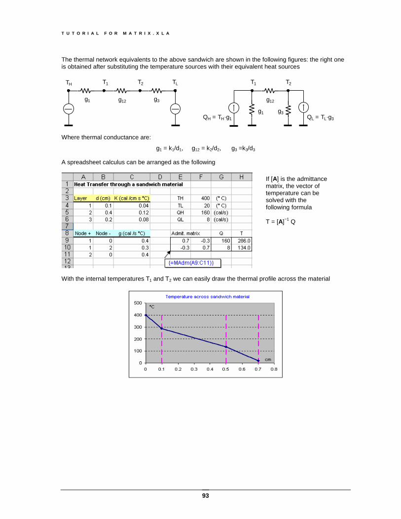
T U T O R I A L F O R M A T R I X . X L A
93
The thermal network equivalents to the above sandwich are shown in the following figures: the right one is obtained after substituting the temperature sources with their equivalent heat sources
T1 T2 TLTH
g1 g12 g3
Where thermal conductance are:
g1 = k1/d1, g12 = k2/d2, g3 =k3/d3 A spreadsheet calculus can be arranged as the following
With the internal temperatures T1 and T2 we can easily draw the thermal profile across the material
If [A] is the admittance matrix, the vector of temperature can be solved with the following formula T = [A]−1 Q
T1 T2
QH = TH·g1
g1
g12
g3QL = TL·g3
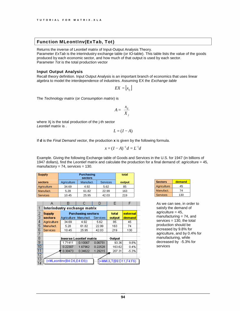
T U T O R I A L F O R M A T R I X . X L A
94
Function MLeontInv(ExTab, Tot) Returns the inverse of Leontief matrix of Input-Output Analysis Theory. Parameter ExTab is the interindustry exchange table (or IO-table). This table lists the value of the goods produced by each economic sector, and how much of that output is used by each sector. Parameter Tot is the total production vector Input Output Analysis Recall theory definition. Input Output Analysis is an important branch of economics that uses linear algebra to model the interdependence of industries. Assuming EX the Exchange table
[ ]ijxEX =
The Technology matrix (or Consumption matrix) is
=
j
ij
Xx
A
where Xj is the total production of the j-th sector Leontief matrix is .
)( AIL −= If d is the Final Demand vector, the production x is given by the following formula.
dLdAIx 11)( −− =−= Example. Giving the following Exchange table of Goods and Services in the U.S. for 1947 (in billions of 1947 dollars), find the Leontief matrix and calculate the production for a final demand of: agricolture = 45, manufactory = 74, services = 130. Supply Purchasing
sectors total
sectors Agriculture Manufact. Services output Agriculture 34.69 4.92 5.62 85 Manufact. 5.28 61.82 22.99 163 Services 10.45 25.95 42.03 219
As we can see, in order to satisfy the demand of agriculture = 45, manufacturing = 74, and services = 130, the total production should be increased by 9.8% for agriculture, and by 0.4% for manufacturing, while decreased by -5.3% for services
Sectors demand Agriculture 45 Manufact. 74 Services 130
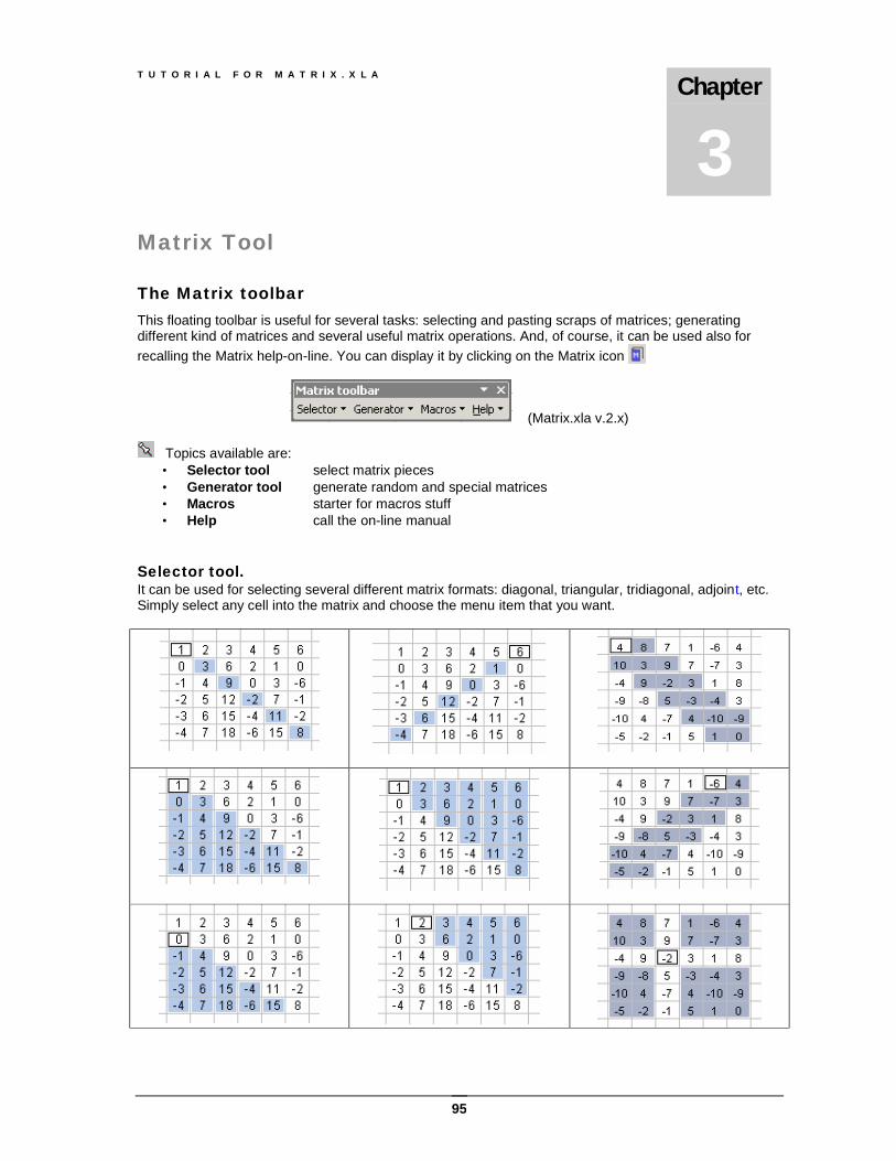
T U T O R I A L F O R M A T R I X . X L A
95
Matrix Tool The Matrix toolbar This floating toolbar is useful for several tasks: selecting and pasting scraps of matrices; generating different kind of matrices and several useful matrix operations. And, of course, it can be used also for recalling the Matrix help-on-line. You can display it by clicking on the Matrix icon
(Matrix.xla v.2.x)
Topics available are: • Selector tool select matrix pieces • Generator tool generate random and special matrices • Macros starter for macros stuff • Help call the on-line manual
Selector tool. It can be used for selecting several different matrix formats: diagonal, triangular, tridiagonal, adjoint, etc. Simply select any cell into the matrix and choose the menu item that you want.
Chapter
3
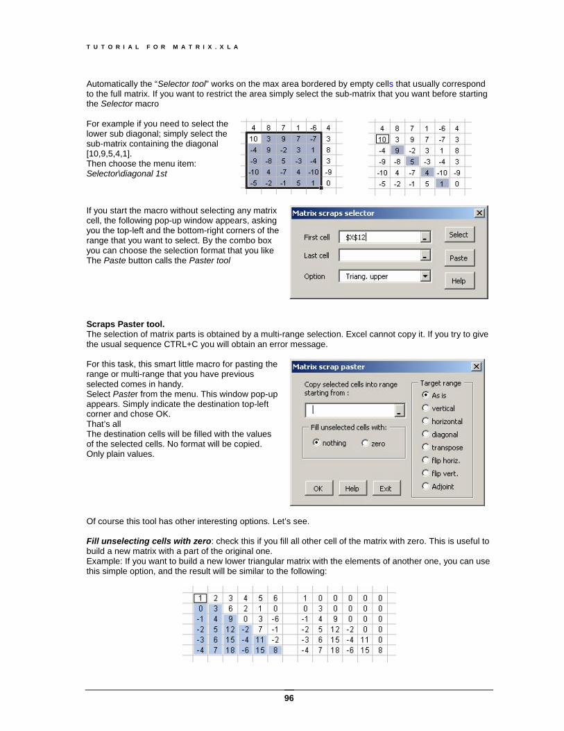
T U T O R I A L F O R M A T R I X . X L A
96
Automatically the “Selector tool” works on the max area bordered by empty cells that usually correspond to the full matrix. If you want to restrict the area simply select the sub-matrix that you want before starting the Selector macro For example if you need to select the lower sub diagonal; simply select the sub-matrix containing the diagonal [10,9,5,4,1]. Then choose the menu item: Selector\diagonal 1st
If you start the macro without selecting any matrix cell, the following pop-up window appears, asking you the top-left and the bottom-right corners of the range that you want to select. By the combo box you can choose the selection format that you like The Paste button calls the Paster tool
Scraps Paster tool. The selection of matrix parts is obtained by a multi-range selection. Excel cannot copy it. If you try to give the usual sequence CTRL+C you will obtain an error message. For this task, this smart little macro for pasting the range or multi-range that you have previous selected comes in handy. Select Paster from the menu. This window pop-up appears. Simply indicate the destination top-left corner and chose OK. That’s all The destination cells will be filled with the values of the selected cells. No format will be copied. Only plain values.
Of course this tool has other interesting options. Let’s see. Fill unselecting cells with zero: check this if you fill all other cell of the matrix with zero. This is useful to build a new matrix with a part of the original one. Example: If you want to build a new lower triangular matrix with the elements of another one, you can use this simple option, and the result will be similar to the following:
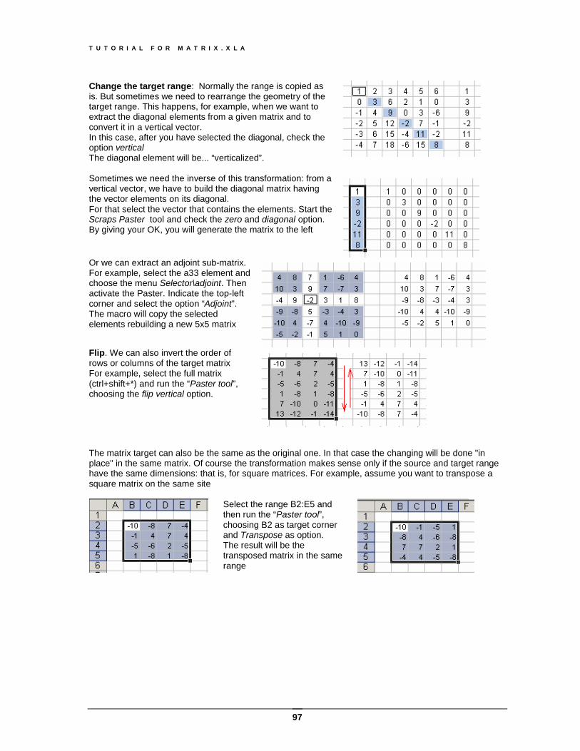
T U T O R I A L F O R M A T R I X . X L A
97
Change the target range: Normally the range is copied as is. But sometimes we need to rearrange the geometry of the target range. This happens, for example, when we want to extract the diagonal elements from a given matrix and to convert it in a vertical vector. In this case, after you have selected the diagonal, check the option vertical The diagonal element will be... “verticalized”.
Sometimes we need the inverse of this transformation: from a vertical vector, we have to build the diagonal matrix having the vector elements on its diagonal. For that select the vector that contains the elements. Start the Scraps Paster tool and check the zero and diagonal option. By giving your OK, you will generate the matrix to the left
Or we can extract an adjoint sub-matrix. For example, select the a33 element and choose the menu Selector\adjoint. Then activate the Paster. Indicate the top-left corner and select the option “Adjoint”. The macro will copy the selected elements rebuilding a new 5x5 matrix
Flip. We can also invert the order of rows or columns of the target matrix For example, select the full matrix (ctrl+shift+*) and run the “Paster tool”, choosing the flip vertical option.
The matrix target can also be the same as the original one. In that case the changing will be done "in place" in the same matrix. Of course the transformation makes sense only if the source and target range have the same dimensions: that is, for square matrices. For example, assume you want to transpose a square matrix on the same site
Select the range B2:E5 and then run the “Paster tool”, choosing B2 as target corner and Transpose as option. The result will be the transposed matrix in the same range
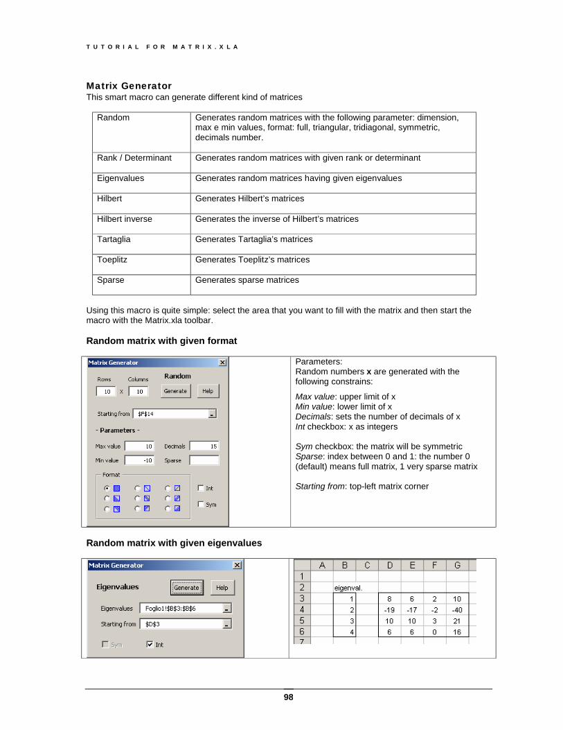
T U T O R I A L F O R M A T R I X . X L A
98
Matrix Generator This smart macro can generate different kind of matrices
Random
Generates random matrices with the following parameter: dimension, max e min values, format: full, triangular, tridiagonal, symmetric, decimals number.
Rank / Determinant
Generates random matrices with given rank or determinant
Eigenvalues
Generates random matrices having given eigenvalues
Hilbert
Generates Hilbert’s matrices
Hilbert inverse
Generates the inverse of Hilbert’s matrices
Tartaglia
Generates Tartaglia’s matrices
Toeplitz Generates Toeplitz’s matrices
Sparse
Generates sparse matrices
Using this macro is quite simple: select the area that you want to fill with the matrix and then start the macro with the Matrix.xla toolbar. Random matrix with given format
Parameters: Random numbers x are generated with the following constrains:
Max value: upper limit of x Min value: lower limit of x Decimals: sets the number of decimals of x Int checkbox: x as integers Sym checkbox: the matrix will be symmetric Sparse: index between 0 and 1: the number 0 (default) means full matrix, 1 very sparse matrix Starting from: top-left matrix corner
Random matrix with given eigenvalues
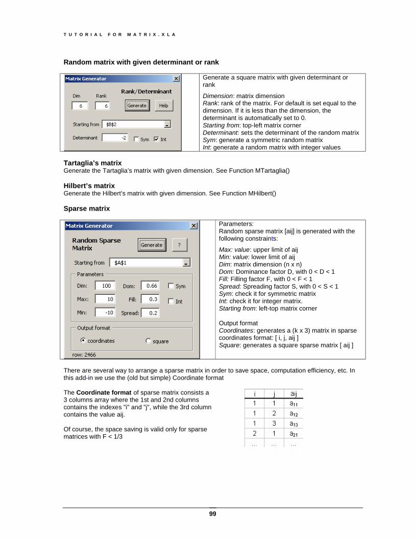
T U T O R I A L F O R M A T R I X . X L A
99
Random matrix with given determinant or rank
Generate a square matrix with given determinant or rank
Dimension: matrix dimension Rank: rank of the matrix. For default is set equal to the dimension. If it is less than the dimension, the determinant is automatically set to 0. Starting from: top-left matrix corner Determinant: sets the determinant of the random matrix Sym: generate a symmetric random matrix Int: generate a random matrix with integer values
Tartaglia’s matrix Generate the Tartaglia’s matrix with given dimension. See Function MTartaglia() Hilbert’s matrix Generate the Hilbert’s matrix with given dimension. See Function MHilbert() Sparse matrix
Parameters: Random sparse matrix [aij] is generated with the following constraints:
Max: value: upper limit of aij Min: value: lower limit of aij Dim: matrix dimension (n x n) Dom: Dominance factor D, with 0 < D < 1 Fill: Filling factor F, with 0 < F < 1 Spread: Spreading factor S, with 0 < S < 1 Sym: check it for symmetric matrix Int: check it for integer matrix. Starting from: left-top matrix corner Output format Coordinates: generates a (k x 3) matrix in sparse coordinates format: [ i, j, aij ] Square: generates a square sparse matrix [ aij ]
There are several way to arrange a sparse matrix in order to save space, computation efficiency, etc. In this add-in we use the (old but simple) Coordinate format The Coordinate format of sparse matrix consists a 3 columns array where the 1st and 2nd columns contains the indexes "i" and "j", while the 3rd column contains the value aij. Of course, the space saving is valid only for sparse matrices with F < 1/3
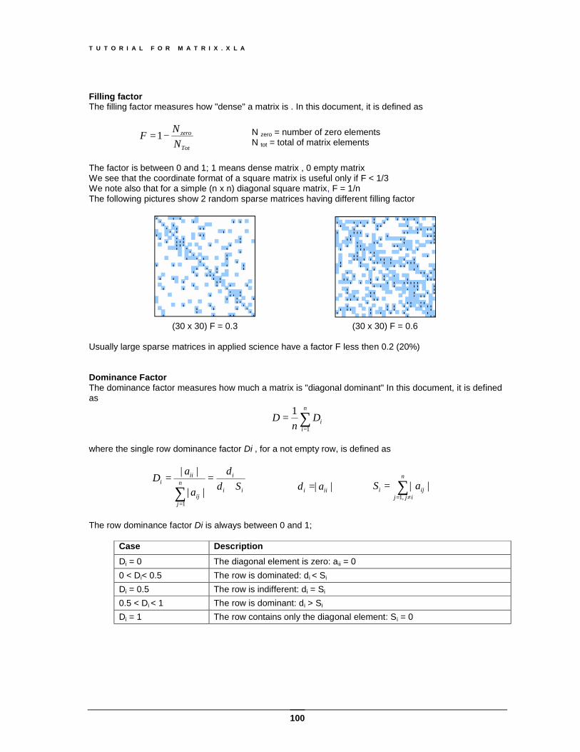
T U T O R I A L F O R M A T R I X . X L A
100
Filling factor The filling factor measures how "dense" a matrix is . In this document, it is defined as
Tot
zero
NNF −=1
N zero = number of zero elements N tot = total of matrix elements
The factor is between 0 and 1; 1 means dense matrix , 0 empty matrix We see that the coordinate format of a square matrix is useful only if F < 1/3 We note also that for a simple (n x n) diagonal square matrix, F = 1/n The following pictures show 2 random sparse matrices having different filling factor
(30 x 30) F = 0.3 (30 x 30) F = 0.6
Usually large sparse matrices in applied science have a factor F less then 0.2 (20%) Dominance Factor The dominance factor measures how much a matrix is "diagonal dominant" In this document, it is defined as
∑=
=n
iiD
nD
1
1
where the single row dominance factor Di , for a not empty row, is defined as
ii
i
ij
n
j
iii Sd
d
a
aD+
==
∑=
| |
||
1
|| iii ad = | |,1
ij
n
ijji aS ∑
≠=
=
The row dominance factor Di is always between 0 and 1;
Case Description Di = 0 The diagonal element is zero: aii = 0 0 < Di< 0.5 The row is dominated: di < Si Di = 0.5 The row is indifferent: di = Si 0.5 < Di < 1 The row is dominant: di > Si Di = 1 The row contains only the diagonal element: Si = 0
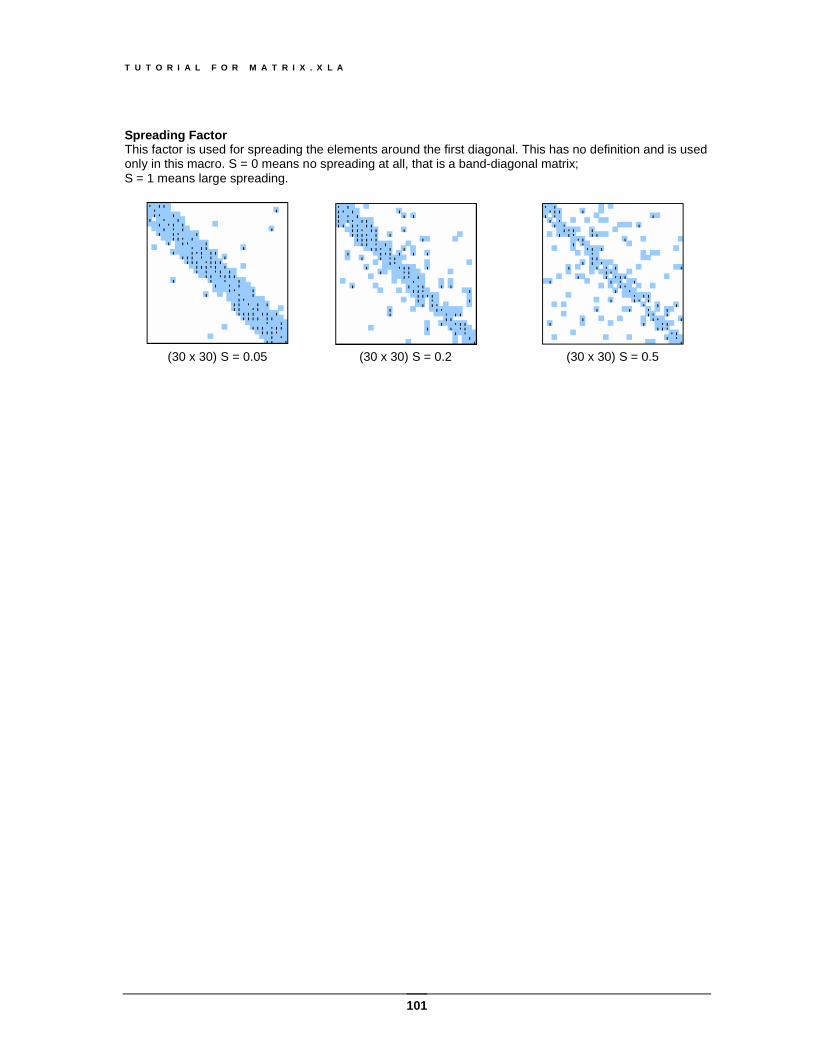
T U T O R I A L F O R M A T R I X . X L A
101
Spreading Factor This factor is used for spreading the elements around the first diagonal. This has no definition and is used only in this macro. S = 0 means no spreading at all, that is a band-diagonal matrix; S = 1 means large spreading.
(30 x 30) S = 0.05 (30 x 30) S = 0.2 (30 x 30) S = 0.5
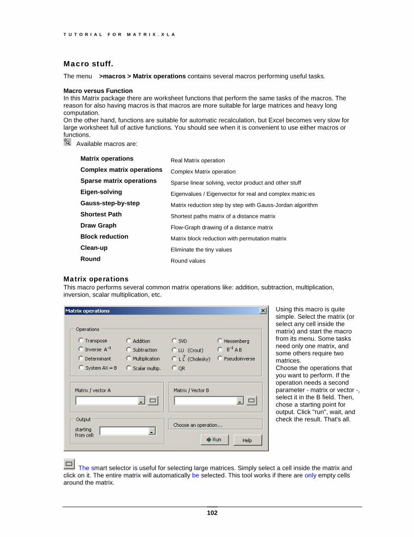
T U T O R I A L F O R M A T R I X . X L A
102
Macro stuff. The menu >macros > Matrix operations contains several macros performing useful tasks. Macro versus Function In this Matrix package there are worksheet functions that perform the same tasks of the macros. The reason for also having macros is that macros are more suitable for large matrices and heavy long computation. On the other hand, functions are suitable for automatic recalculation, but Excel becomes very slow for large worksheet full of active functions. You should see when it is convenient to use either macros or functions.
Available macros are:
Matrix operations Real Matrix operation Complex matrix operations Complex Matrix operation Sparse matrix operations Sparse linear solving, vector product and other stuff Eigen-solving Eigenvalues / Eigenvector for real and complex matric ies Gauss-step-by-step Matrix reduction step by step with Gauss-Jordan algorithm Shortest Path Shortest paths matrix of a distance matrix Draw Graph Flow-Graph drawing of a distance matrix Block reduction Matrix block reduction with permutation matrix Clean-up Eliminate the tiny values Round Round values
Matrix operations This macro performs several common matrix operations like: addition, subtraction, multiplication, inversion, scalar multiplication, etc.
Using this macro is quite simple. Select the matrix (or select any cell inside the matrix) and start the macro from its menu. Some tasks need only one matrix, and some others require two matrices. Choose the operations that you want to perform. If the operation needs a second parameter - matrix or vector -, select it in the B field. Then, chose a starting point for output. Click "run", wait, and check the result. That's all.
The smart selector is useful for selecting large matrices. Simply select a cell inside the matrix and click on it. The entire matrix will automatically be selected. This tool works if there are only empty cells around the matrix.
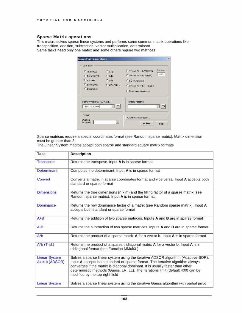
T U T O R I A L F O R M A T R I X . X L A
103
Sparse Matrix operations This macro solves sparse linear systems and performs some common matrix operations like: transposition, addition, subtraction, vector multiplication, determinant Same tasks need only one matrix and some others require two matrices
Sparse matrices require a special coordinates format (see Random sparse matrix). Matrix dimension must be greater than 3. The Linear System macros accept both sparse and standard square matrix formats Task Description
Transpose Returns the transpose. Input A is in sparse format
Determinant Computes the determinant. Input A is in sparse format
Convert Converts a matrix in sparse coordinates format and vice versa. Input A accepts both standard or sparse format
Dimensions Returns the true dimensions (n x m) and the filling factor of a sparse matrix (see Random sparse matrix). Input A is in sparse format.
Dominance Returns the row dominance factor of a matrix (see Random sparse matrix). Input A accepts both standard or sparse format
A+B Returns the addition of two sparse matrices. Inputs A and B are in sparse format
A-B Returns the subtraction of two sparse matrices. Inputs A and B are in sparse format
A*b Returns the product of a sparse matrix A for a vector b. Input A is in sparse format
A*b (Trid.) Returns the product of a sparse tridiagonal matrix A for a vector b. Input A is in tridiagonal format (see Function MMult3 )
Linear System Ax = b (ADSOR)
Solves a sparse linear system using the iterative ADSOR algorithm (Adaptive-SOR). Input A accepts both standard or sparse format. The Iterative algorithm always converges if the matrix is diagonal dominant. It is usually faster than other deterministic methods (Gauss. LR, LL). The iterations limit (default 400) can be modified by the top-right field
Linear System Solves a sparse linear system using the iterative Gauss algorithm with partial pivot
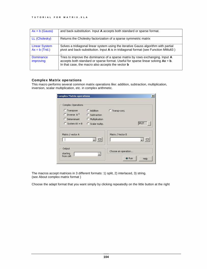
T U T O R I A L F O R M A T R I X . X L A
104
Ax = b (Gauss) and back-substitution. Input A accepts both standard or sparse format.
LL (Cholesky) Returns the Cholesky factorization of a sparse symmetric matrix
Linear System Ax = b (Trid.)
Solves a tridiagonal linear system using the iterative Gauss algorithm with partial pivot and back-substitution. Input A is in tridiagonal format (see Function MMult3 ) ..
Dominance improving
Tries to improve the dominance of a sparse matrix by rows exchanging. Input A accepts both standard or sparse format. Useful for sparse linear solving Ax = b. In that case, the macro also accepts the vector b
Complex Matrix operations This macro performs several common matrix operations like: addition, subtraction, multiplication, inversion, scalar multiplication, etc. in complex arithmetic.
The macros accept matrices in 3 different formats: 1) split, 2) interlaced, 3) string. (see About complex matrix format ) Choose the adapt format that you want simply by clicking repeatedly on the little button at the right
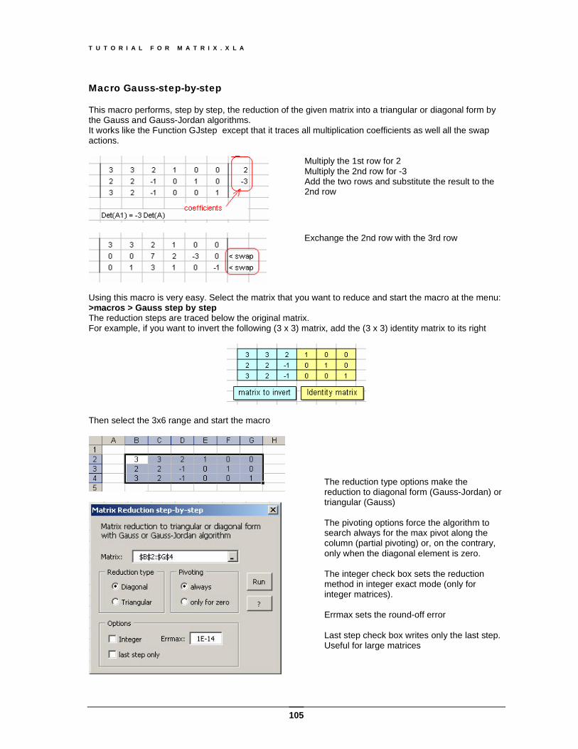
T U T O R I A L F O R M A T R I X . X L A
105
Macro Gauss-step-by-step This macro performs, step by step, the reduction of the given matrix into a triangular or diagonal form by the Gauss and Gauss-Jordan algorithms. It works like the Function GJstep except that it traces all multiplication coefficients as well all the swap actions.
Multiply the 1st row for 2 Multiply the 2nd row for -3 Add the two rows and substitute the result to the 2nd row
Exchange the 2nd row with the 3rd row
Using this macro is very easy. Select the matrix that you want to reduce and start the macro at the menu: >macros > Gauss step by step The reduction steps are traced below the original matrix. For example, if you want to invert the following (3 x 3) matrix, add the (3 x 3) identity matrix to its right
Then select the 3x6 range and start the macro
The reduction type options make the reduction to diagonal form (Gauss-Jordan) or triangular (Gauss) The pivoting options force the algorithm to search always for the max pivot along the column (partial pivoting) or, on the contrary, only when the diagonal element is zero. The integer check box sets the reduction method in integer exact mode (only for integer matrices). Errmax sets the round-off error Last step check box writes only the last step. Useful for large matrices
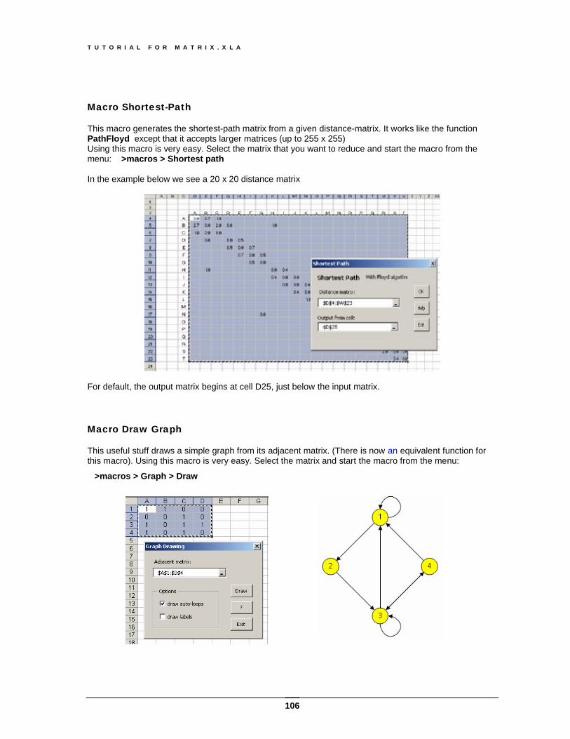
T U T O R I A L F O R M A T R I X . X L A
106
Macro Shortest-Path This macro generates the shortest-path matrix from a given distance-matrix. It works like the function PathFloyd except that it accepts larger matrices (up to 255 x 255) Using this macro is very easy. Select the matrix that you want to reduce and start the macro from the menu: >macros > Shortest path In the example below we see a 20 x 20 distance matrix
For default, the output matrix begins at cell D25, just below the input matrix. Macro Draw Graph This useful stuff draws a simple graph from its adjacent matrix. (There is now an equivalent function for this macro). Using this macro is very easy. Select the matrix and start the macro from the menu:
>macros > Graph > Draw
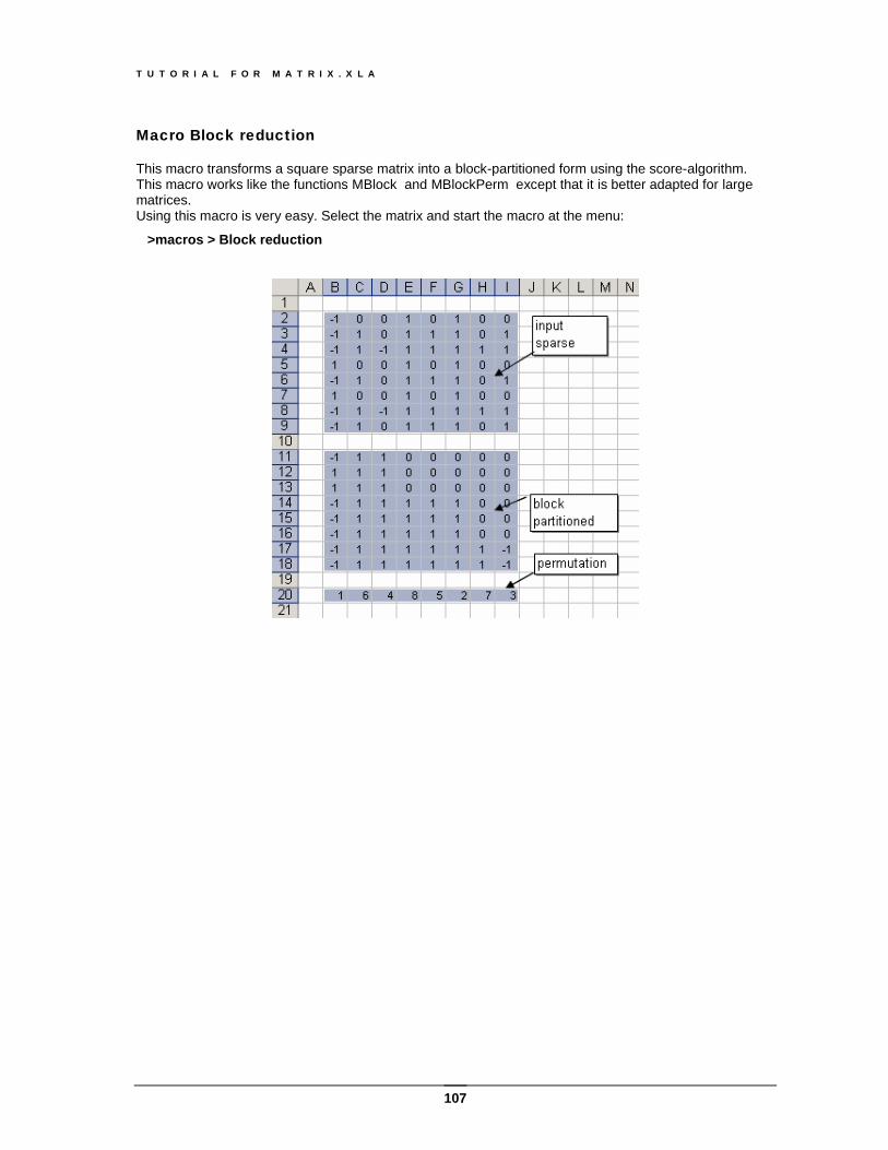
T U T O R I A L F O R M A T R I X . X L A
107
Macro Block reduction This macro transforms a square sparse matrix into a block-partitioned form using the score-algorithm. This macro works like the functions MBlock and MBlockPerm except that it is better adapted for large matrices. Using this macro is very easy. Select the matrix and start the macro at the menu:
>macros > Block reduction
108
References In this chapter we have collected, listed for subject, all the documents that we have consulted without regarding their source (paper books, electronics books, html web pages, pdf notes, etc.). For all internet documents we have used the web engine GOOGLE . "LAPACK -- Linear Algebra PACKage" 3.0, Update: May 31, 2000
"Numerical Analysis" F. Sheid, McGraw-Hill Book Company, New-York, 1968
"Numerical Recipes in FORTRAN 77- The Art of Scientific Computing" - 1986-1992 by Cambridge University Press. Programs Copyright (C) 1986-1992 by Numerical Recipes Software
"Matrix Analysis and Applied Linear Algebra", C. D. Mayer, Siam, 2000 "Nonlinear regression", Gordon K. Smyth, John Wiley & Sons, 2002, Vol. 3, pp 1405-1411
"Linear Algebra" vol 2 of Handbook for Automatic Computation, Wilkinson, Martin, and Peterson, 1971
“Linear Algebra” Jim Hefferon, Saint Michael’s College, Colchester (Vermont), July 2001.
“Linear Algebra - Answers to Exercises” Jim Hefferon, Saint Michael’s College, Colchester ( Vermont), July 2001
“Calcolo Numerico” Giovanni Gheri, Università degli Studi di Pisa, 2002
“Introduction to the Singular Value Decomposition” by Todd Will, UW-La Crosse, University of Wisconsin, 1999
“Calcul matriciel et équation linéaires”, Jean Debord, Limoges Cedex, 2003
“Leontief Input-Output Modelling” Addison-Wesley, Pearson Education
“Computational Linear Algebra with Models”, Gareth Williams, (Boston: Allyn and Bacon, 1978), pp. 123-127.
“Scalar, Vectors & Matrices”, J. Walt Oler, Texas Teach University, 1980
EISPACK Guide, “Matrix Eigensystem Routines”, Smith B. T. at al. 1976
"Numerical Methods that usually work", F. S. Acton, The Mathematical Association of America, 1990
"Analysis Nunerical Methods", E. Isaacson, H. B. Keller, Wiley & Sons, 1966
"Calculo Numérico", Neide M. B. Franco, 2002
"Metodos Numericos" Sergio R. De Freitas, 2000
"Numerical Mathematics in Scientific Computation", G. Dahlquist, Å. Björck, vol II.
"Advanced Excel for scientific data analysis" , Robert de Levie, Oxford University Press, 2004

109
Credits Manu thanks to: Gregory Klein,
Bernard Wagner
and Carlos Aya
The library FunCustomize.dll, appears by courtesy of Laurent Longre (http://longre.free.fr)
Many thanks are also due to Prof. Robert de Levie for numerous corrections and valuable comments.

110
WHITE PAGE

111
2006, by Foxes Team ITALY
Dic. 2006