Matrices and Systems of Linear Equationsstecher/LinearAlgebraPdfFiles/...Chapter 1 Matrices and Systems of Linear Equations In Chapter 1 we discuss how to solve a system of linear

Chapter 1

Matrices and Systems of

Linear Equations

In Chapter 1 we discuss how to solve a system of linear equations. If there arenot too many equations or unknowns our task is not very difficult; what welearned in high school will suffice. Fortunately our world is fairly complicated.We quite often meet problems that can be reduced to solving a system of severalhundred or more equations with an equally large number of unknowns. Thus ourmethod of solution should simplify the bookkeeping involved and be as directand straightforward as possible. This simplification process leads in a naturalmanner to objects called matrices and various rules for manipulating them.

A great amount of time and effort will be spent on matrices, but we alwaysneed to keep in mind that we are discussing systems of linear equations.

1.1 Systems of Linear Equations

Let’s look at a simple example of a system of linear equations:

2x1 + 3x2 = 6−x1 + 4x2 = 8

(1.1)

The problem is to determine all possible pairs of numbers, which we denote byx1 and x2, such that these numbers will satisfy both equations in (1.1). Thetrick (technique) in solving (1.1) is to first remove one of the unknowns fromone of the equations. To accomplish this, multiply the second equation by 2 andthen add the resulting equation to the first. This gives us the following system:

11x2 = 22−x1 + 4x2 = 8

(1.2)

This system of equations is easy to solve. Clearly x2 = 2211 = 2, and replacing

x2 with 2 in the second equation we have −x1 + 4(2) = 8 or −x1 = 0. Hence,

1

2 CHAPTER 1. MATRICES AND SYSTEMS OF LINEAR EQUATIONS

x1 = 0. We now check that we have actually found a solution to our originalsystem (1.1). That is, we replace x1 by 0 and x2 by 2 and verify that bothequations are satisfied.

Let’s go back to the beginning and try to reduce some of the work involved.We started with (1.1), but now instead of writing the unknowns every time let’sjust write the coefficients. This leads us to

2x1 + 3x2 = 6−x1 + 4x2 = 8

List coefficients

2 3 : 6−1 4 : 8

2R2 +R1 0 11 : 22−1 4 : 8

R1 ↔ R2 −1 4 : 80 11 : 22

−R1 1 −4 : −8111R2 0 1 : 2

(1.3)

The notation is almost self-explanatory. For example, 2R2+R1 means multiplythe second row (equation) by 2 and then add it to the first row, which gives usa new first row (equation). R1 ↔ R2 means interchange the first and secondrows. −R1 and 1

11R2 mean multiply the first row by −1 and the second rowby 1

11 . The colons are used to distinguish the right-hand side of equations (1.3)from the coefficients of the unknowns. Later we will not bother with the colons.

The next step in our procedure is to realize that the final array in (1.3)represents the equations

x1 − 4x2 = −8x2 = 2

(1.4)

From (1.4) we again get the solution x2 = 2, x1 = −8+ 8 = 0. The form of thisfinal array should be noted; namely, there are ones in the “main diagonal” andzeros below it, which means that we can easily solve for x2 and then x1.

Let’s look at one more specific example before discussing linear systems ingeneral.

Example 1.

2x1 + 3x2 − x3 = 6−4x1 + x3 = 7

x2 − 2x3 = 1(1.5)

Remember that we’re going to delete the variables and manipulate the rows inorder to arrive at the following form if possible

1 . . : b10 1 . : b20 0 1 : b3

(1.6)

1.1. SYSTEMS OF LINEAR EQUATIONS 3

From (1.5) we have

2 3 −1 : 6−4 0 1 : 70 1 −2 : 1

2R1 +R2

2 3 −1 : 60 6 −1 : 190 1 −2 : 1

R2 ↔ R3

2 3 −1 : 60 1 −2 : 10 6 −1 : 19

−6R2 +R3

2 3 −1 : 60 1 −2 : 10 0 11 : 13

1

2R1

1

11R3

13

2R3 −1

2: 3

0 1 −2 : 1

0 0 1 :13

11

(1.7)

With this last array we associate the following system:

x1 +3

2x2 −

1

2x3 = 3

x2 − 2x3 = 1 (1.8)

x3 =13

11

Since the leading coefficients are one, we can easily solve this system for x3 = 1311 ,

x2 = 1+2(1311 ) =3711 , and x1 = 3+ 1

2x3− 32x2 = 3+(12 )(

1311 )−(32 )(

3711 ) = − 16

11 . Theease with which (1.8) is solved demonstrates why the form in (1.6) is desirable.

�

Question: The numbers x1, x2, and x3 satisfy (1.8). Do they also satisfy(1.5)? They had better! The fact that they do can be demonstrated by eitherputting these numbers into equations (1.5) or observing that the row operations,which were performed, are all reversible. For example, the reverse (inverse) of−6R2 + R3 would be 6R2 + R3. Starting with the final array of (1.7), if weexecute the sequence of operations 11R3, 2R1, 6R2 +R3, R3 ↔ R2, −2R1+R2,we will get the original array. Since (1.8) may be algebraically manipulatedto get (1.5), every solution of (1.8) will also satisfy (1.5), and conversely everysolution of (1.5) will also be a solution of (1.8).

We next discuss the form of a general system of m linear equations in n


unknowns:a11x1 + a12x2 + · · ·+ a1nxn = b1a21x2 + a22x2 + · · ·+ a2nxn = b2. . . . . . . . . . . . . . . . . . . . . . . . . . . . . . . . . . .am1x1 + am2x2 + · · ·+ amnxn = bm

(1.9)

Thus symbols x1, x2, . . . , xn represent the unknowns that we are trying tofind. The aij , 1 ≤ i ≤ m, 1 ≤ j ≤ n, are called the coefficients of the system. Itis assumed that the coefficients aij and the terms bj, 1 ≤ j ≤ m, are all known.A few words about the subscripts are in order. The first subscript, i, of aijrefers to the equation in which this term appears, while the second subscript,j, tells us which of the n unknowns aij multiplies. Thus, if a23 = 6 we knowthat the variable x3 in the second equation is multiplied by 6. To make surethis convention is understood, let’s go back to (1.5):

2x1 + 3x2 − x3 = 6−4x1 + x3 = 7

x2 − 2x3 = 1(1.5)

For the above system of equations we would have

a11 = 2 a12 = 3 a13 = −1 b1 = 6a21 = −4 a22 = 0 a23 = 1 b2 = 7a31 = 0 a32 = 1 a33 = −2 b3 = 1

One more bit of terminology. The procedure we’ve been using is referred to asGaussian elimination. We summarize it below.

1. List the coefficients only.

2. Use row operations to obtain zeros below the “main diagonal.”

3. Solve the new system.

The phrase “main diagonal” in 2 above refers to those aij for which i = j.

Example 2.

x1 + x2 − x3 = 1x1 + x3 = 0[

1 1 −1 : 11 0 1 : 0

]

−R1 +R2

[

1 1 −1 : 10 −1 2 : −1

]

−R2

[

1 1 −1 : 10 1 −2 : 1

]

−R2 +R1

[

1 0 1 : 00 1 −2 : 1

]

This last matrix implies that

x1 = −x3 x2 = 1 + 2x3 �


Here we did not get numbers for an answer, but equations relating two ofthe unknowns to the third. This means that we have an infinite number ofsolutions, a different one for each choice of x3. For example, if we set x3 = 0,then x1 = 0 and x2 = 1 is a solution. Similarly the triple x3 = 1, x2 = 3,x1 = −1 is also a solution.

Example 3.

x1 + x2 = 1x2 + 3x3 = 4

x1 + 2x2 + 3x3 = 6

1 1 0 : 10 1 3 : 41 2 3 : 6

−R1 +R3

1 1 0 : 10 1 3 : 40 1 3 : 5

−R2 +R3

1 1 0 : 10 1 3 : 40 0 0 : 1

Now what?This last array represents the system of equations:

x1 + x2 = 1

x2 + 3x3 = 4

0x1 + 0x2 + 0x3 = 1

Clearly the third equation has no solution, which means that our original systemcan have no solution. �

These examples indicate that for an arbitrary linear system we may haveone of three possibilities:

1. No solution: Example 3

2. Exactly one solution: Example 1

3. An infinite number of solutions: Example 2

It is not clear that these are the only possibilities. For example, is therea system with exactly two solutions or some other finite number? We shallsee later that this cannot happen, and that the above three cases are the onlypossible ones.

Before concluding this first section we discuss in the next example the ge-ometry of systems of equations, at least in two unknowns.


Example 4. Sketch the solutions of each of the following systems of equations:

a. 2x1 + x2 = 1 4x1 + 2x2 = 2

x2

4x1 + 2x2 = 2

2x1 + x2 = 1

x1

( 12, 0)

(0, 1)

The locus of points that satisfy this system is a straight line as shownabove.

b. 2x1 + x2 = 1

x1 − x2 = 0

x2

x1 − x2 = 0

x1

2x1 + x2 = 1

( 13, 13)

The locus of points that satisfy both equations is all points common toboth straight lines. In this case there is only one such point, namely,x1 = 1

3 = x2.

c. 2x1 + x2 = 1

2x1 + x2 = 4

2x1 + x2 = 1

x2

2x1 + x2 = 4

x1


Each equation describes a straight line, and these lines are parallel. Sincethey do not intersect, the system of equations has no solution. �

Problem Set 1.1

1. Find all solutions, if any, of the following systems of linear equations:

a. −3x1 − 6x2 = 02x1 + 4x2 = 0

b. −3x1 − 6x2 = 32x1 + 4x2 = 2

2. Solve the following systems of linear equations:

a. 2x1 + 3x2 = 7−6x1 + x2 = 1

b. 2x1 + 3x2 = b1−6x1 + x2 = b2

3. Find all solutions, if any, of the following systems of linear equations:

a. 2x1 + x2 − x3 = 1x1 + x2 + x3 = 2

b. 2x1 + x2 − x3 = 1x1 + x2 + x3 = 2x1 − x2 = 2

4. Find all numbers k such that the following system of equations has asolution and then solve that system.

2x1 + x2 − x3 = 1

x1 + x2 + x3 = 2

3x1 + 2x2 = k

5. Find all solutions of the following system of linear equations:

2x1 + 3x2 − x3 + x4 = 2

x1 + x2 + x3 − 2x4 = −6

x1 + 2x3 + 4x4 = 13

2x2 + x3 − x4 = −5

6. Find all solutions of the following system:

x1 − x3 + x4 = 0

4x1 + x3 + 2x4 = 0

x1 + 2x2 − x3 − x4 = 0

2x2 + 5x3 − 4x4 = 0


7. Matt’s, Dave’s, and Abe’s ages are not known but are related as follows:The sum of Dave’s and Abe’s ages is 3 more than Matt’s. Matt’s age plusAbe’s age is 9 more than Dave’s. If the sum of their ages is 35, how old isAbe?

8. Granny’s favorite recipe for pecan pie calls for 1 cup of pecans, 3 cupsof sugar, and 3 eggs. Her recipe for one batch of pecan puffs calls for 1cup of sugar, 1 cup of pecans, and 2 eggs. If she has 2 pounds of pecans,6 pounds of sugar, and a henhouse next door (i.e., as many eggs as sheneeds), how many pecans pies and batches of pecan puffs can she makewhile using up all her supplies? (1 pound = 2 cups)

9. Two cars are traveling toward each other. The first is moving at a speedof 45 mph and the second at 65 mph. If, at the start, they are 35 milesapart, how long before they meet and how far will each car have traveled?

10. Find all solutions of the following system:

2x1 + x3 + 6x4 = 0−x1 + 3x2 + 4x3 + 2x4 = 0

x2 + 3x3 + 4x4 = 1x1 + x2 − x3 − x4 = 1

11. Find all solutions of the following system of equations:

2x1 + 2x2 + x4 = 0x1 − x2 + 2x3 + x4 = 1x1 + x2 + 4x4 = 1

12. If possible, solve the following systems of equations:

a. 3x1 − 2x2 + 3x3 = 0 x1 + x2 + x4 = 0 x1 − x3 − x4 = 0

b. x1 − x2 = 1 x1 + x2 − x3 = −2 x1 − 5x2 + 2x3 = 1

13. Dabs cement plant makes mortar and cement. Each ton of mortar requires12 ton of lime and 1

5 ton of sand. Each ton of cement requires 13 ton of

lime and 34 ton of sand. If Dabs has 9 tons of lime and 11 tons of sand

available, how many tons of mortar and cement can the company make?

14. Graph the solution sets for each of the following systems of equations.Since there are two unknowns, the solution set is the set consisting of allpairs of numbers (x1, x2) that satisfy the equations

a. x1 − 2x2 = 62x1 + x2 = 1

b. 3x1 + 4x2 = 1


15. Graph the solution sets of the following systems of equations. Here, thesolution set consists of those triples of numbers (x1, x2, x3) that satisfythe equations

a. x1 + x2 + x3 = 0

b. x1 + x2 + x3 = 0 x1 + x3 = 0

c. x1 + x2 + x3 = 0 x1 + x3 = 0 x1 − x3 = 0

16. Find an equation for the straight line that passes through the followingpoints:

a. (1, 6), (−1, 4)

b. (−2, 6), (4, 3)

17. Is there a straight line that passes through the following sets of points?

a. (1, 6), (−1, 4), (3, 7)

b. (−4, 2), (3, 7), (1, 8)

18. Find an equation for the circle that passes through the three points (−4, 2),(3, 7), (1, 8).

19. Find the solution set to the equations

a. x1 + x2 = 0

b. x1 + x2 = 1

c. Graph the solution sets of a and b. How are they related?

20. Suppose we have an infinite sequence of numbers xk, k = 1, 2, . . . , thatare related to each other by the equations xk+1 = 2xk.

a. Find a formula for xk in terms of x1. For example, x2 = 2x1 andx3 = 4x1.

b. Suppose the xk are related by the equation xk+2 = xk + xk+1. Thusx3 = x1 + x2 and x4 = x2 + x3 = x1 + 2x2. Can you find a formulafor xk(k > 3) in terms of x1 and x2?

21. Suppose we have two sequences of numbers xk and yk for k = 1, 2, . . . ,and that the sequences are related by the equations

xk+1 = xk + yk

yk+1 = xk − yk

Find a formula for xk and yk in terms of x1 and y1 for all k if you can.If you cannot discover such a formula, compute x3 and y3 in terms of x1and y1.


1.2 Matrices

In the preceding section the first step taken in solving a system of equationswas to remove the variables, which left us with a rectangular array of numbers.These arrays are given a special name.

Definition 1.1. An m× n matrix is a rectangular array of numbers arrangedin m rows and n columns.

In most of this book we use real numbers, but from time to time, as the incli-nation or need arises, complex number will appear.

Example 1.

A =

[

1 23 4

]

is a 2× 2 matrix

B =

[

13

]

is a 2× 1 matrix

C =

1 0 −1 64 0 1 01 0 0 0

is a 3× 4 matrix �

We will often denote an m × n matrix A by writing A = [aij ], 1 ≤ i ≤ m,1 ≤ j ≤ n. The symbol aij is used to indicate the entry in the ith row andjth column. Thus, counting from the top left corner of the matrix, the firstsubscript tells us which row and the second subscript which column the entryappears in.

Example 2.

A =

[

1 23 4

]

a11 = 1, a12 = 2a21 = 3, a22 = 4

B =

[

13

]

b11 = 1b21 = 3

C =

1 5 −1 64 0 −2 81 2 3 4

c11 = 1, c12 = 5, c13 = −1, c14 = 6c22 = 0, c23 = −2, c24 = 8

c33 = 3, c34 = 1�

There are various operations that we may perform involving matrices, andwe will spend the next few pages defining and exemplifying them. Before doingso, however, we need to state clearly what it means to say that two matricesare equal. Let A and B be two matrices. We say A = B if they are of the samesize and their corresponding entries are equal. For example, the matrices

[

1 20 1

]

and

[

1 21 1

]

1.2. MATRICES 11

are not equal since the entries in the second row and first column are not equal.The matrices

[

1 20 1

]

and[

1 2]

are not equal since the first is a 2× 2 matrix and the second is a 1× 2 matrix.A precise definition of matrix equality is:

Definition 1.2. Let A = [aij ], 1 ≤ i ≤ m, 1 ≤ j ≤ n. Let B = [bij ], 1 ≤ i ≤ p,1 ≤ j ≤ q, be two matrices. We say A = B if and only if m = p, n = q, andaij = bij for each i and j.

One algebraic operation involving matrices is that of addition. Given twomatrices of the same size, we form their sum by adding together their respectiveentries. Thus

[

1 2−1 3

]

+

[

0 14 6

]

=

[

1 33 9

]

and[

1 2 6]

+[

1 −1 4]

=[

2 1 10]

A formal definition of matrix addition is:

Definition 1.3. Let A = [aij ], 1 ≤ i ≤ m, 1 ≤ j ≤ n. Let B = [bij ], 1 ≤ i ≤ m,1 ≤ j ≤ n. The sum S = A+B of these two m×n matrices is the m×n matrixwhose i, j entry, sij , equals aij + bij .

Example 3.

a.

[

1 −2 3−7 0 4

]

+

[

6 −2 61 −8 0

]

=

[

7 −4 9−6 −8 4

]

b.

[

−1 12

3 5

]

+

[

12 01 −2

]

=

[

− 12

12

4 3

]

�

There are also times when we wish to multiply a matrix by a number. To dothis, just multiply every entry in the matrix by that number. For example,

2

[

−1 14 3

]

=

[

−2 28 6

]

Definition 1.4. Let A = [aij ] be any m× n matrix and c any number. ThencA is the m× n matrix whose i, j entry is caij .

Example 4.

a. 2

1 −14 31 20 8

=

2 −28 62 40 16

b. −1

[

1 −23 4

]

=

[

−1 2−3 −4

]

�


As with real or complex numbers, these two operations satisfy certain laws,which we state in the following theorem:

Theorem 1.1. Let A = [aij ], B = [bij ], and C = [cij ] be any m× n matrices.Let a and b be any numbers. Then the following properties hold:

1. A+B = B +A

2. (A+B) + C = A+ (B + C)

3. a(A+B) = aA+ aB

4. (a+ b)A = aA+ bA

5. a(bA) = (ab)A

Proof. The proofs of these statements are straightforward, and we shall gothrough the details of properties 1 and 3 only

1. A+B = [aij ] + [bij ]

= [aij + bij ] = [bij + aij ]

= B +A

3. a(A+B) = a([aij ] + [bij ])

= a([aij + bij ])

= [a(aij + bij)]

= [aaij + abij ]

= [aaij ] + [abij ]

= a[aij ] + a[bij ]

= aA+ aB

The next example repeats the above computations using particular matricesand numbers.

Example 5.

3

([

1 2 0−1 6 7

]

+

[

−1 −1 40 5 8

])

= 3

[

0 1 4−1 11 15

]

=

[

0 3 12−3 33 45

]

3

[

1 2 0−1 6 7

]

+ 3

[

−1 −1 40 5 8

]

=

[

3 6 0−3 18 21

]

+

[

−3 −3 120 15 24

]

=

[

0 3 12−3 33 45

]

�

1.2. MATRICES 13

We see that our answer does not depend upon whether we first add and thenmultiply, or multiply and then add.

There is a special m×n matrix, called the zero matrix, which we denote byOmn (when the size is clear we will drop the subscripts). This matrix has all itsentries equal to zero. Thus,

O21 =

[

00

]

and O22 =

[

0 00 0

]

It is clear that the following is true:

Theorem 1.2. Let A be any m× n matrix. Then

1. A+Omn = A

2. 0A = Omn

Our next task is to learn how to multiply matrices. The rule at first seemsunusual, but after we relate it in the next section to systems of equations, itwill be clear that we are not being unreasonable. The first thing to rememberis that two arbitrary sized matrices A and B cannot be multiplied together toform AB. The number of columns in the first factor A must equal the numberof rows in the second factor B. To calculate the i, j entry of AB, we multiplythe entries of the ith row of A by the corresponding entries of the jth columnof B, and then sum these products. For example, if

A =

[

1 2−4 3

]

B =

[

−26

]

then AB will be the 2× 1 matrix C, where

C =

[

c11c21

]

=

[

(first row of A) “times” (first column of B)(second row of A) “times” (first column of B)

]

or2× 2 2× 1 2× 1

[

1 2−4 3

] [

−26

]

=

[

(1)(−2) + (2)(6)(−4)(−2) + (3)(6)

]

=

[

1026

]

The precise definition of matrix multiplication is:

Definition 1.5. Let A = [aij ] be an m × n matrix. Let B = [bij ] be an n× pmatrix. Then AB = C = [cij ] is an m× p matrix where

cij = ai1b1j + ai2b2j + · · ·+ ainbnj

=

n∑

k=1

aikbkj

Note the respective sizes of these matrices:


(m× n)(n× p) = m× p

The number of columns in A must equal the number of rows in B. The numberof rows in AB is the same as the number of rows in A and the number ofcolumns in AB is the same as the number of columns in B. Readers unfamiliarwith summation notation should refer to Appendix B. Figure 1.1 illustrates thisdefinition.

...

...ai1 · · · ain

...

...

b1jb2j...

· · · bij · · ·...bnj

=

...

...· · · cij · · ·

...

...

where

cij = ai1b1j + ai2b2j + · · ·+ ainbnj

Figure 1.1

Example 6.

a.

[

1 1 04 3 6

]

1 −1 6−2 0 38 1 2

=

[

1− 2 + 0 −1 + 0 + 0 6 + 3 + 04− 6 + 48 −4 + 0 + 6 24 + 9 + 12

]

=

[

−1 −1 946 2 45

]

Note that we cannot multiply these two matrices in opposite order sincethe number of columns (three) in the second matrix does not equal thenumber of rows (two) in the first matrix.

b.

[

0 11 0

] [

2 31 4

]

=

[

0 + 1 0 + 42 + 0 3 + 0

]

=

[

1 42 3

]

Multiplying these matrices in the opposite order, we have

c.

[

2 31 4

] [

0 11 0

]

=

[

0 + 3 2 + 00 + 4 1 + 0

]

=

[

3 24 1

]

Note that the products in b and c are not equal. Thus, even though AB andBA are both defined, they may not be equal. �

Matrix multiplication does satisfy some algebraic laws, which are stated in thefollowing theorem:

1.2. MATRICES 15

Theorem 1.3. Let A,B, and C denote matrices of appropriate size; that is, ifwe write AB, then A has the same number of columns as B has rows. Let a beany real number. Then the following formulas hold:

1. (A+B)C = AC +BC,A(B + C) = AB +AC

2. (AB)C = A(BC)

3. a(AB) = aA(B) = A(aB)

Proof. Let A = [aij ] be an m × n matrix, B = [bij ] be an m × n matrix, andC = [cij ] be an n× p matrix. Then

(A+B)C = [aij + bij ][cij ]

=

[

n∑

k=1

(aik + bik)ckj)

]

=

[

n∑

k=1

aikckj +

n∑

k=1

bikckj

]

=

[

n∑

k=1

aikckj

]

+

[

n∑

k=1

bikckj

]

= AC +BC

The proof that A(B + C) = AB + AC is essentially the same as that for(A + B)C = AC + BC; so we omit it. Properties 2 and 3 may be proved in asimilar manner, and the reader is asked to do so in the problems at the end ofthis section.

We’ve seen that there is a zero matrix Omn. There is also an identity matrixIn which plays the role of the number 1 in matrix multiplication. The n × nmatrices, In, are defined as follows:

I1 = [1] I2 =

[

1 00 1

]

I3 =

1 0 00 1 00 0 1

For an arbitrary natural number n we define

In = [δij ]

where δij =

{

1 if i = j

0 if i 6= j

That is, the symbol δij , which is called the Kronecker delta, is equal to 1 if iequals j and zero if the subscripts are different.


Example 7. Let A =

[

a bc d

]

be any 2× 2 matrix. Show that I2A = AI2 = A.

I2A =

[

1 00 1

] [

a bc d

]

=

[

a+ 0 b+ 00 + c 0 + d

]

=

[

a bc d

]

= A

AI2 =

[

a bc d

] [

1 00 1

]

=

[

a+ 0 0 + bc+ 0 0 + d

]

=

[

a bc d

]

= A �

Theorem 1.4. Let A be an m×n matrix. Let In and Im denote the n×n andm×m identity matrices, respectively. Then

ImA = AIn = A

Proof. Let A = [aij ]. Then

ImA = [δij ][aij ] =

[

m∑

k=1

δikakj

]

= [aij ] = A

Since δij = 0 unless k = i, the sum of the m terms δikakj has only one nonzerosummand, the one for which k = i. Similarly AIn = A. Note that if A is asquare n× n matrix, InA = AIn = A.

By this time the reader should have the feeling that if a rule is true fornumbers it is also true for matrices. This feeling should be maintained with twoimportant exceptions:

1. AB 6= BAThis does not mean that AB always differs from BA but rather that equalityneed not hold.

2. AB = AC does not imply that B = CThe reader will find examples of this in the problems at the end of this section.

There is one other operation that we need to discuss. It’s called taking thetranspose of a matrix. The operation is very simple to perform. We merelyinterchange rows and columns; that is, the ith row of A become the ith columnof AT (A transpose). For example, if

A =

[

1 −1 04 2 −6

]

then

AT =

1 4−1 20 −6

Definition 1.6. Let A = [aij ] be an m×nmatrix. The transpose of A, denotedby AT = [aTij ], is an n×m matrix where

aTij = aji

1.2. MATRICES 17

In the future rather than write

1−124

we will write[

1 −1 2 4]T

.

Example 8.

1.

[

1 23 4

]T

=

[

1 32 4

]

2.[

1 2 3]T

=

123

3.

1 2 4 0−1 −2 0 36 2 1 0

T

=

1 −1 62 −2 24 0 10 3 0

�

The following theorem, whose proof we omit, is stated for future reference.

Theorem 1.5. Let A and B be two matrices. Then

(AB)T = BTAT

Example 9. Let A =

[

1 20 3

]

and B =

[

−1 03 4

]

. Verify Theorem 1.5 for these

two matrices.

(AB)T =

([

1 20 3

] [

−1 03 4

])T

=

[

5 89 12

]T

=

[

5 98 12

]

BTAT =

[

−1 30 4

] [

1 02 3

]

=

[

5 98 12

]

�

Definition 1.7. A square matrix A is said to be symmetric if A = AT . Thusa 2× 2 matrix

A =

[

a bc d

]

is symmetric if and only if c = b.

Problem Set 1.2

1. Let A =

[

1 2 3−1 0 −2

]

and let B =

[

−1 6 −4−2 −3 0

]

. Compute the fol-

lowing matrices:


a. 3A b. A−B c. 2A+ 3B

2. Perform the indicated operations.

a. 2

[

6 7 1 1−1 3 1 −1

]

b. −2

[

1 6 06 −1 1

]

+

[

−2 4 −1−1 −2 −1

]

c.

6 −1 4−2 1 −33 1 00 2 5

−

2 3 −20 1 11 0 16 2 −1

3. Let A =

[

1 24 −3

]

. Let B =

[

−1 00 3

]

. Compute the following:

a. AB b. BA c. 2A−B

4. Let A =

[

2 2 1−3 6 1

]

. Let B =

1 0 −1−2 1 46 0 3

. Compute if possible the

following matrix products: AB, BA, A2 = AA, and B2 = BB.

5. Compute the following products:

a.

[

1 02 1

] [

3 64 9

]

b.

[

3 64 9

] [

1 02 1

]

6. Let A =

[

1 6−1 2

]

. Are there any numbers x1 and x2 such that if B =[

x1 01 x2

]

, then AB = BA?

7. For each of the matrices below compute A2 and A3. Note A2 = AA andA3 = AA2 = A2A.

a.

[

1 00 2

]

b.

[

1 10 2

]

c.

[

a bc d

]

8. Find all numbers k such that the matrix K =

[

k 1 + k1− k −k

]

satisfies the

equation K2 = I2.

9. If A =

[

a bc d

]

, show that A2 =

[

0 10 0

]

is not possible for any choice of

a, b, c, or d.

1.2. MATRICES 19

10. Let D =

[

d 00 d

]

, where d is an arbitrary number. Show that DA = AD

for any 2 × 2 matrix A. Conversely show that if D is a matrix for whichAD = DA for every 2× 2 matrix A, then D has the above form for somenumber d. Such matrices are called scalar matrices.

11. Let A =

[

2 −14 1

]

. Let B =

[

2 3 61 −1 0

]

. Do there exist matrices X or Y

such that the equations AX = B or Y A = B have solutions?

12. Let A =

1 0 00 2 00 0 3

and let B =

1 1 00 −2 00 0 3

. Compute the following

matrices:

a. A2, B2, AB,BA

b. AT , BT

c. A3, B3

d. A4, B4

13. Let A be an arbitrary n× n matrix. Define A0 = In, A1 = A, A2 = AA,

and An+1 = AAn, for n = 1, 2, 3, . . . . Show that if p and q are arbitrarynonnegative integers then ApAq = Ap+q. Thus, we may conclude thatApAq = AqAp. (Hint: Use induction.)

14. Let A =

[

1 12 4

]

, B =

0 21 4

−1 −1

, C =

[

6 0 1−4 1 0

]

, D =

[

−1 0 1−2 −2 3

]

.

Calculate, when defined, each of the following matrices:

a. 2A+B, 2C −D,B +D b. AB,BA c. A2, B2 d. AT , BT

15. Let A =

[

2 1 34 2 6

]

, B =

112

. Show (AB)T = BTAT .

16. Let A =

[

−1 64 5

]

, X =[

1 2]

. Show that (XAT )T = AXT .

17. Prove properties 2 and 3 of Theorem 1.3.

18. Let A =

[

−1 64 3

]

, B =

[

7 5−2 1

]

. Verify that A[

7 −2]T

is the first

column of AB and that A[

5 1]T

is the second column of AB.

19. Let A and B be the matrices in problem 18. Verify that[

−1 6]

B is the

first row of AB and that[

4 3]

B is the second row of AB.

20. Show that


a.

[

2 −16 7

] [

x1x2

]

= x1

[

26

]

+ x2

[

−17

]

b.[

x1 x2]

[

2 −16 7

]

= x1[

2 −1]

+ x2[

6 7]

21. Let A be any 3 × 3 matrix whose last row has only zeros. Let B be any3× 3 matrix. Show that the third row of AB has only zeros in it.

22. Generalize problem 21.

23. Which of the following matrices is symmetric?

a.

[

1 −11 2

]

b.

1 6 46 1 −14 −1 2

c.

−1 0 40 4 64 6 2

24. Let A and B be two m× n matrices. Show that (A+B)T = AT +BT .

25. Show that (AT )T = A, for any matrix A.

26. Verify Theorem 1.5 for the matrices in problem 3.

27. Prove Theorem 1.5 for A, any 2× 2 matrix, and B, any 2× 3 matrix.

28. Show that if A and B are symmetric matrices of the same size, then(AB)T = BA. Find two symmetric 2× 2 matrices A and B such that ABis symmetric; then find two more 2×2 symmetric matrices such that theirproduct is not symmetric.

29. Show that if A and B are symmetric, then so is A+B.

30. Prove Theorem 1.5 for A an arbitrary 2×3 matrix and B any 3×1 matrix.

31. An n× n matrix is upper triangular if aij = 0 when i > j, that is, all theterms below the main diagonal are zero. Show that the sum and productof two upper triangular matrices of the same size are also upper triangular.

32. A matrix is said to be lower triangular if its transpose is upper triangular.Show that a matrix is lower triangular if and only if aij = 0 when i < j.Show that the sum and product of two lower triangular matrices are alsolower triangular.

33. Show that AAT and ATA are symmetric for any matrix A.

34. Prove Theorem 1.2.

35. Let

A =

[

2 −13 − 3

2

]

B =

[

0 1−5 3

]

C =

[

−1 −3−7 −5

]

Show that AB = AC. Thus, it is possible for AB = AC with A differentfrom the zero matrix and B not equal to C.

1.3. ELEMENTARY ROW OPERATIONS 21

1.3 Elementary Row Operations

In this section we discuss in more detail the basic ideas involved in Gaussianelimination, and how one systematically reduces a matrix to the form (1.6).

The operations used in Gaussian elimination are called the elementary rowoperations. There are three of them which we list below.

Definition 1.8. The three elementary row operations are:

1. Interchange any two rows.

2. Multiply a row by a nonzero constant.

3. Add a multiple of one row to another.

The following example illustrates these three operations.

Example 1. Let A =

4 1 0−1 2 38 −2 5

a. Interchange rows 1 and 2 of A:

R1 ↔ R2

4 1 0−1 2 38 −2 5

⇒

−1 2 34 1 08 −2 5

b. Multiply row 3 of A by 18 :

18R3

4 1 0−1 2 38 −2 5

⇒

4 1 0−1 2 3

1 −1

4

5

8

c. Add four times the second row of A to the first row.

4R2 +R1

4 1 0−1 2 38 −2 5

⇒

0 9 12−1 2 38 −2 5

�

Definition 1.9. Let A and B be two m × n matrices. We say that B isrow equivalent to A if there is a sequence of elementary row operations thattransforms A into B.


Example 2a. Let A =

[

2 41 3

]

. Show that I2 =

[

1 00 1

]

is row equivalent to A.

R1 ↔ R2

[

2 41 3

]

⇒[

1 32 4

]

−2R1 +R2

[

1 32 4

]

⇒[

1 30 −2

]

− 12R2

[

1 30 −2

]

⇒[

1 30 1

]

−3R2 +R1

[

1 30 1

]

⇒[

1 00 1

]

�

Thus, the sequence of row operations R1 ↔ R2, −2R1 + R2, − 12R2, and

(−3R2 +R1) performed in the given order transforms A into I2. �

Example 2b. Show that the matrix A above is row equivalent to I2.

Solution. We know there is a sequence of elementary row operations that trans-forms A into I2, and we expect that the row operations that undo the effectof these operations should then transform I2 into A. The operations we usedabove and their “inverses” are

R1 ↔ R2 R1 ↔ R2

−2R1 + R2 2R1 +R2

− 12R2 −2R2

−3R2 + R1 3R2 +R1

Performing the row operations in the second column in reverse order upon I2we have

3R2 +R1

[

1 00 1

]

⇒[

1 30 1

]

−2R2

[

1 30 1

]

⇒[

1 30 −2

]

2R1 +R2

[

1 30 −2

]

⇒[

1 32 4

]

R1 ↔ R2

[

1 32 4

]

⇒[

2 41 3

]

= A

�

The previous example is a particular case of a general fact.

Lemma 1.1. Given any sequence of elementary row operations that transformsA into B, there is another sequence that transforms B into A. This is the sameas saying that if B is row equivalent to A, then A is row equivalent to B.


Proof. We first show that each elementary row operation has a correspondingelementary row operation that cancels the effect of the first operation. Thus,let A be an arbitrary m× n matrix. Suppose

Rj ↔ Rk A⇒ B

That is, rows j and k of A are interchanged, and the resulting matrix is B.Clearly if we interchange the same two rows, then we transform B back into A.We also have:

If cRj : A⇒ B, then (1/c)Rj : B ⇒ A

If cRj +Rk : A⇒ B, then − cRj +Rk : B ⇒ A

Now suppose B is row equivalent to A. Then there is a sequence of elementaryrow operations E1, . . . , Em which when performed in the given order, that is,Em followed by Em−1, . . . , followed by E1, transforms A into B. Let Fj denotethe “inverse” of Ej . Thus, if E1 is 2R3, then F1 is 1

2R3. Then Fm, . . . , F1 whenperformed on B, in this order, will transform B into A; cf. Example 2.

The following theorem lists some properties of row equivalence:

Theorem 1.6. Let A,B, and C be m× n matrices, Then:

a. A is row equivalent to itself.

b. If A is row equivalent to B, then B is row equivalent to A.

c. If A is row equivalent to B and B is row equivalent to C, then A is rowequivalent to C.

Proof. Part a is obvious, and b is Lemma 1.1. To see that c is true, let E1, . . . , Ep

denote a sequence of elementary row operations that transform A into B. LetF1, . . . , Fq denote a sequence of elementary row operations that transform Binto C. Clearly the following sequence of row operations, F1, . . . , Fq, E1, . . . , Ep,transform A into C. Properties a, b, and c are called reflexivity, symmetry, andtransitivity, respectively.

A more explicit description of what we meant by (1.6) is:

Definition 1.10. The matrix A is said to be in row echelon form if it satisfiesthe following conditions:

1. All rows consisting entirely of zeros must be at the bottom of the matrix;i.e., no row of zeros may precede any row that has a nonzero entry.

2. The first nonzero entry of any row must be the number 1.

3. All entries directly below the first nonzero entry of any row must be zero.

4. The number of the column containing the first nonzero entry of a rowmust increase as we move down the rows of the matrix.


Example 3.

a. The matrix

[

1 0 10 3 0

]

is not in row echelon form since the first nonzero

entry in row 2 is not a 1. If row 2 is divided by 3, we get the row equivalentmatrix

[

1 0 10 1 0

]

which is in row echelon form.

b.

[

0 0 00 1 0

]

is not in row echelon form but the matrix

[

0 1 00 0 0

]

which comes from the preceding matrix after a row interchange is in rowechelon form.

c.

1 1 0 10 1 1 10 1 0 0

is not in row echelon form, since there is a nonzero entry

in the 3,2 position, which is directly below the first nonzero entry of row2.

d.

1 0 00 0 10 1 0

is not in row echelon form, since condition 4 of Definition 1.10

is not satisfied by this matrix. The first nonzero terms do not move to theright as we go down the rows. �

Definition 1.11. A matrix is said to be in reduced row echelon form if it is inrow echelon form and also satisfies:

5. All entries above the first nonzero entry of any row are zero.

Example 4.

a.

[

1 1 00 1 0

]

is in row echelon form, but not in reduced row echelon form.[

1 0 00 1 0

]

is in reduced row echelon form.

b.

1 0 10 1 00 1 1

is in neither row echelon form nor reduced row echelon form.

Condition 3 does not hold for this matrix.

c.

1 0 20 1 10 0 0

is in reduced row echelon form. �


We next state two theorems but do not give their proofs.

Theorem 1.7. Every matrix is row equivalent to a unique matrix in reducedrow echelon form.

Theorem 1.8. Two matrices are row equivalent if and only if they are rowequivalent to the same matrix in reduced row echelon form.

In general if we wish to determine whether or not two matrices are row equiva-lent, we use row operations to find the reduced row echelon form they are rowequivalent to, and then compare these two forms.

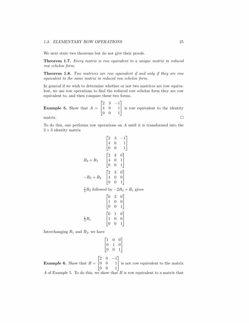
Example 5. Show that A =

2 3 −14 0 10 0 1

is row equivalent to the identity

matrix. �

To do this, one performs row operations on A until it is transformed into the3× 3 identity matrix

2 3 −14 0 10 0 1

R3 +R1

2 3 04 0 10 0 1

−R3 +R2

2 3 04 0 00 0 1

14R2 followed by −2R2 +R1 gives

0 3 01 0 00 0 1

13R1

0 1 01 0 00 0 1

Interchanging R1 and R2, we have

1 0 00 1 00 0 1

Example 6. Show that B =

2 0 −10 0 10 0 1

is not row equivalent to the matrix

A of Example 5. To do this, we show that B is row equivalent to a matrix that


cannot be row equivalent to I3. We deduce from this, via Theorem 1.8, that Aand B cannot be row equivalent.

2 0 −10 0 10 0 1

R3 +R1

2 0 00 0 10 0 1

−R2 +R3

2 0 00 0 10 0 0

12R1

1 0 00 0 10 0 0

�

Since the last matrix is in reduced row echelon form, and I3 is also in reducedrow echelon form, Theorem 1.7 implies B cannot be row equivalent to I3, andhence B cannot be row equivalent to A. For if B were row equivalent to A, thenby Theorem 1.8 and Example 3, B would be row equivalent to I3. Actuallythere was no need to perform any row operations on B at all, since it is clearfrom the structure of B that no sequence of row operations can put a 1 in itssecond column.

For each of the elementary row operations there is a corresponding elemen-tary column operation. For the most part, however, when solving systems oflinear equations, only the elementary row operations are used.

The reader should also know that each of the elementary row (column)operations has an elementary row (column) matrix associated with it. Forexample, if we are dealing with 3×n matrices, then the elementary row matrixassociated with a particular elementary row operation is that matrix whichresults when the given elementary row operation is performed upon I3.

1. R1 ↔ R2 :

1 0 00 1 00 0 1

⇒

0 1 01 0 00 0 1

2. cR2 :

1 0 00 1 00 0 1

⇒

1 0 00 c 00 0 1

3. cR2 +R3 :

1 0 00 1 00 0 1

⇒

1 0 00 1 00 c 1

These examples demonstrate the relationship between the elementary row op-eration and its associated matrix. If we are in the class of m×n matrices (3× 3above), we would start out with Im; i.e., the number of columns is irrelevant.


Example 7. Let A be any 3×3 matrix. Let E be the elementary matrix associ-ated with 2R1+R3. Show that EA equals the matrix obtained by transformingA with this row operation.

Solution. The matrix E, obtained by transforming I3 with 2R1 +R3, equals

1 0 00 1 02 0 1

Computing EA for an arbitrary 3× 3 matrix, we have

EA =

1 0 00 1 02 0 1

a b cd e fg h i

=

a b cd e f

2a+ g 2b+ h 2c+ i

and

2R1 +R3 :

a b cd e fg h i

⇒

a b cd e f

2a+ g 2b+ h 2c+ i

= EA �

The equality demonstrated in this example is not a coincidence. It is true ingeneral, and the reader is asked to show this in the problems at the end of thissection.

Example 8. Let A =

2 4 84 3 15 0 2

. Let E =

1 0 0−2 1 0− 5

2 0 1

. Show that the first

column of the matrix product EA equals[

2 0 0]T

. Note that E is the matrixproduct

E =

1 0 00 1 0

−5

20 1

1 0 0−2 1 00 0 1

That is, E is the result of applying the two elementary row operations−2R1+R2

and − 52R1 +R3 consecutively to I3.

EA =

1 0 0−2 1 0

−5

20 1

2 4 84 3 15 0 2

=

2 4 80 − 5 −150 −10 −18

Thus, EA equals the matrix that results from applying the above two rowoperations to A. �

Problem Set 1.3

1. Which of the following matrices are in row echelon form?


a.

[

0 11 2

]

,

[

1 −20 1

]

,

[

0 01 0

]

,

[

1 00 0

]

b.

1 1 1 00 1 1 30 0 1 0

,

0 1 2 40 0 0 10 0 1 6

,

1 1 0 −60 1 1 10 0 0 1

2. Which of the following matrices are in reduced row echelon form?

a.

[

0 11 2

]

,

[

1 −20 1

]

,

[

0 01 0

]

,

[

1 00 0

]

b.

1 1 1 00 1 1 30 0 1 0

,

0 1 2 40 0 0 10 0 1 6

,

1 1 0 −60 1 1 10 0 0 1

c.

1 2 0 0 10 0 1 2 80 0 0 0 1

,

1 2 0 0 00 0 1 2 00 0 0 0 1

3. Find the reduced row echelon form to which each of the following matricesis row equivalent.

a.

[

6 12 4

]

,

[

−1 23 −6

]

b.

1 −2 04 0 63 0 8

,

6 − 5 13 1 43 −13 10

c.

1 2 8 −12 0 4 −23 0 1 1

4. Find the reduced row echelon form to which each of the following matricesis row equivalent.

a.

[

6 −21 4

]

b.

[

3 31 1

]

5. Find the reduced row echelon form of each of the following matrices:

a.

1 2−4 −85 6

10 12

b.[

−4 3 6 −8]

c.

−4237

d.

[

9 2 8 4 56 1 0 3 −2

]

6. For each of the following elementary row operations, write the 3 × 3 ele-mentary row matrix that corresponds to it.

a. 2R2 +R3 b. R1 ↔ R3 c. −3R2


7. For each of the following sequences of row operations find a 2× 2 matrixE such that, if A is any 2× 3 matrix, EA equals the matrix derived fromA after the given sequence of row operations is performed on A.

a. R1 ↔ R2, 2R2 +R1

b. −R1 +R2, 2R1 +R2, 3R2 +R1

8. Let E be the matrix

[

0 11 0

]

. We know that if A is any 2 × 2 matrix

then EA is the matrix we get after interchanging the first two rows of A.Describe EA in terms of A.

9. Let E =

[

1 −20 1

]

. Let A be any 2 × 2 matrix. What column operations

performed upon A will produce the product matrix AE?

10. If E is the m×m elementary matrix that corresponds to multiplying rowi by c, then EA is the matrix we get when row i of A is multiplied by c.Show this for m = 2 or 3. How is AE related to A?

11. If E is the m × m elementary matrix that corresponds to interchangingrow i with row j, then EA is the matrix we get when rows i and j of Aare interchanged. Show this for m = 2 or 3. How is AE related to A?

12. An n × n matrix D = [dij ] is said to be a diagonal matrix if dij = 0whenever i 6= j. That is, the only nonzero entries of D are on the main

diagonal. Let D equal

[

−1 00 2

]

. For each of the following matrices, A,

compute DA and AD.

a.

[

4 00 3

]

b.

[

2 01 0

]

c.

[

2 10 0

]

13. Let D =

d1 0 00 d2 00 0 d3

, E =

e1 0 00 e2 00 0 e3

. Compute DE.

14. Let A be an arbitrary 3×3 matrix, and let D be any 3×3 diagonal matrix.Describe the rows of DA and the columns of AD.

15. Let A = [ajk] be any 3× 3 matrix for which a11 is not zero. Let E be the

matrix

1 0 0−a21/a11 1 0−a31/a11 0 1

. Describe the first column of EA.

16. How many different 2× 2 matrices in reduced row echelon form are there?Find at least four.


17. Let A =

[

a bc d

]

. SupposeE is a 2×2 matrix such thatEA =

[

a+ c b + dc d

]

.

Clearly E =

[

1 10 1

]

is one such matrix. Are there any others?

18. For which 2× 2 diagonal matrices D is there at least one nonzero matrixA such that DA is the 2× 2 zero matrix?

19. Find all 2× 2 matrices A such that AB is symmetric, where B =

[

1 00 0

]

.

1.4 Matrices and Linear Equations

In this section we show how to write a system of linear equations as a matrixequation, and then demonstrate that the elementary row operations do notchange the solution set.

Let’s take a simple system of linear equations and rewrite it as an equationinvolving matrices.

2x1 + 6x2 = 5−x1 + 3x2 = 4

(1.10)

Let A =

[

2 6−1 3

]

and let X =

[

x1x2

]

. Then we can write (1.10) as

AX =

[

2 6−1 3

] [

x1x2

]

=

[

54

]

(1.11)

Now let’s write the general linear system of m equations in n unknowns:

a11x1 + a12x2 + · · ·+ a1nxn = b1a21x1 + a22x2 + · · ·+ a2nxn = b2. . . . . . . . . . . . . . . . . . . . . . . . . . . . . . . . . . .am1x1 + am2x2 + · · ·+ amnxn = bm

(1.12)

as a matrix equation.Let A = [aij ], X = [x1, . . . , xn]

T , and B = [b1, . . . , bm]T . The matrix A willbe referred to as the coefficient matrix of (1.12) and X as the unknown solutionIf some of the bj are nonzero, B is called the nonhomogeneous term. We see,keeping in mind the definitions of matrix multiplication and equality, that (1.12)can be written as

AX = B (1.13)

Another matrix associated with (1.12) is

A =

a11 a12 . . . a1n b1a21 a22 . . . a2n b2. . . . . . . . . . . . . . . . . . . . . . . . . .am1 am2 . . . amn bm

(1.14)

1.4. MATRICES AND LINEAR EQUATIONS 31

It is called the augmented matrix of (1.12). Notice that the augmented matrixA is just the coefficient matrix A with the right-hand side of (1.12) added onas an (n+ 1)st column.

We want to show that if we have a system of equations and change it to asecond system by performing some elementary row operations, we have neitherlost nor gained any solutions. That is, the solution sets for the two systems arethe same.

Theorem 1.9. Let A and B be the augmented matrices of two systems oflinear equations. If A and B are row equivalent, the two systems have the samesolutions sets.

Proof. Since A and B are row equivalent only if there is a sequence of elementaryrow operations that transforms A into B, it suffices to prove this theorem in thecase where only one of the three elementary row operations is used.

Case 1. Suppose two rows of A, when interchanged, yield B. Clearly all thatwe’ve done is to write the equations in a different order. Hence the solutions toboth of these systems must coincide.

Case 2. Some row of A when multiplied by a nonzero constant yields B. Herewe’ve multiplied one of the equations of the first system by a nonzero constant.This too leaves the solution set invariant.

Case 3. Suppose cRj is added to Rk; that is, the kth row of B is c times thejth row of A added to the kth row of A. Suppose the numbers x1, x2, . . . , xnsatisfy the first system. In particular this means

aj1x1 + · · ·+ xjnxn = bj

ak1x1 + · · ·+ aknxn = bk

Adding c times the first equation to the second equation gives us the followingpair of equations:

aj1x1 + · · ·+ ajnxn = bj

(caj1 + ak1)x1 + · · ·+ (cajn + akn)xn = cbj + bk

But the coefficients of these two equations are the jth and kth rows of B,respectively. Since the remaining m− 2 rows of A and B are equal, we see thatthese n numbers xi also satisfy the second system. Moreover since −cRj + Rk

when performed upon B will yield A, a similar argument shows that everysolution to the second system is also a solution to the first system

Example 1. Solve the following system of equations by finding a matrix in rowechelon form which is row equivalent to the augmented matrix.

2x1 − x2 + x4 = −1

x2 + x3 + x4 = 0

x1 + x2 + x3 = 6


The augmented matrix is

2 −1 0 1 −10 1 1 1 01 1 1 0 6

and it is row equivalent to the following matrices:

R1 ↔ R3

1 1 1 0 60 1 1 0 02 −1 0 1 −1

−2R1 + R3

1 1 1 0 60 1 1 1 00 −3 −2 1 −13

3R2 +R3

1 1 1 0 60 1 1 1 00 0 1 4 −13

The above matrix is in row echelon form. The system of equations for which itis the augmented matrix has as solutions:

x3 = −13− 4x4x2 = 13 + 3x4x1 = 6 + x4

(1.15)

If a numerical value for x4 is specified, setting x1, x2, and x3 equal to thosenumbers which satisfy (1.15) gives us a solution to the original system of equa-tions. Moreover, every solution may be generated in this manner. We obtaintwo explicit solutions by setting x4 equal to 0 and then 1:

(6, 13,−13, 0) (7, 16,−17, 1) �

As usual let A = [aij ] and X = [x1, . . . , xn]T be m× n and n× 1 matrices,

respectively. Let B = [b1, . . . , bm]T be an m× 1 matrix.

Definition 1.12. A system of equations AX = B is said to be homogeneous ifB = Om1, i.e., b1 = 0, b2 = 0, . . . , bm = 0. The zero solution to a homogeneoussystem is called the trivial solution. If B 6= Om1, the system is said to benonhomogeneous.

The following result, which is almost obvious, is extremely useful.

Theorem 1.10. Let A and B be as above. If Xp is any solution to AX = B,every other solution to AX = B can be written in the form X = H+Xp, whereH is a solution to the associated homogeneous equation AX = Om1.

Proof. Suppose AX = B. Set H = X − Xp. Clearly X = Xp + (X − Xp) =Xp +H . Moreover AH = A(X −Xp) = AX −AXp = B −B = Om1.


Note also that if AH = Om1, then A(Xp +H) = AXp +AH = B +Om1 = B.

Example 2. Write the solutions to the system of equations in Example 1 inthe form H +Xp.

Solution. From (1.15) one particular solution (obtained by setting x4 equal tozero), is (6, 13,−13, 0). Thus, we have

X =

613

−130

+ x4

13

−41

= Xp +H

where H equals x4(1, 3,−4, 1)T . It is easy to show that, no matter what valuex4 is given, H is a solution to the homogeneous system. �

Later we will need to know that every homogeneous system of equationswith more unknowns than equations always has a nontrivial solution, that is, asolution for which not all the xj ’s are zero. Before proving this, we look at aspecific example.

Example 3. Show that the following system has a nontrivial solution (twoequations—three unknowns).

3x1 + 2x2 = 0−2x1 + x2 − x3 = 0

Solution. Writing the coefficient matrix, we have[

3 2 0−2 1 −1

]

This matrix is row equivalent to

1 02

7

0 1 −3

7

This matrix implies that x1 = − 27x3 and x2 = 3

7x3 are the only solutions to thesystem. Clearly there are many nontrivial solutions. One is obtained by settingx3 equal to 1, another by setting x3 equal to 2, etc. �

Theorem 1.11. Let A = [aij ] be an m×n matrix with m < n (more unknownsthan equations). Then there is a nontrivial solution to the homogeneous equationAX = Om1.

Proof. We prove this by induction on the number of equations. Suppose firstthat m = 1, i.e., only one equation.

a1x1 + a2x2 + · · ·+ anxn = 0 (1.16)


Since we have an equation, at least one of the coefficients aj is not zero. Supposea1 6= 0. Set x2 = 1 and x3 = · · · = xn = 0. Setting x1 = −a2/a1 gives usa nontrivial solution to (1.16). Now suppose that the theorem is true for pequations, 1 ≤ p < m. Using this we show that the theorem must be true form equations. Let A1 be the matrix in reduced row echelon form that is rowequivalent to A. To show that AX = Om1 has a nontrivial solution it sufficesto show that A1X = Om1 has a nontrivial solution.

Case 1. Assume A1 has no row of zeros. Then there are exactly m columnswith the number 1 as the only nonzero entry. Let xi1 , xi2 , . . . , xim , 1 ≤ i1 <i2 < · · · < im ≤ n be the unknowns associated with these columns. Let k beany integer, 1 ≤ k ≤ n, not equal to any of the ij , 1 ≤ j ≤ m. Set xk = 1. Setall the other variables, excepting the xij , equal to 0. Solve the resulting systemfor the remaining m unknowns xij . Since xk = 1, we have a nontrivial solutionto our homogeneous system.

Case 2. A1 has a row of zeros. This means that A1X = Om1 is actually asystem of p equations with p < m. By our induction hypothesis this system hasa nontrivial solution.

We conclude this section with two examples of how matrices may arise fromdifferent problems.

Example 4. Suppose that a rabbit store starts out with 5 male rabbits and 4female rabbits. Suppose also that every 6 months each female rabbit gives birthto 3 male rabbits and 3 female rabbits. How many male and female rabbits willthere be (assuming no deaths) after 2 years?

Solution. We need to express how many males and females we have duringany 6-month time period. Let mk and fk represent the number of males andfemales, respectively, during the kth time period. Then the following equationsdescribe how the rabbit population grows from one time period to the next:

mk+1 = mk + 3fk

fk+1 = fk + 3fk

Thus[

mk+1

fk+1

]

=

[

1 30 1 + 3

] [

mk

fk

]

Let A be the matrix

[

1 30 4

]

. We have

[

mk+1

fk+1

]

= A

[

mk

fk

]

= A2

[

mk−1

fk−1

]

= · · · = Ak+1

[

m0

f0

]

= Ak+1

[

54

]


For a proof of this by induction see Appendix A. Thus, after 2 years or fourtime periods, we have

[

m4

f4

]

= A4

[

54

]

The reader is asked to complete this example by computing A4. �

Example 5. Suppose we have some system that can be in any one of threedifferent states, which are denoted by S1, S2, and S3. The system is such thatit can pass directly from some states to other states, as Figure 1.2 indicates.The diagram tells us that from S1 the system can either stay in S1 or enter S2.From S3

S2S1

S3

Figure 1.2

it must enter S1 or S2, and once the system is in S2 it cannot leave. We catalogthese data in a matrix T = [tjk]. T is often referred to as a transition matrix.The tjk are defined by

tjk = 1, if the system can pass directly from state j to k.

tjk = 0, if the system cannot pass directly from state j to state k.

Thus T equals

1 1 00 1 01 1 0

Notice that the third column has all zeros; this is because the system can neverenter the third state. We note too that each row must have at least one nonzeroentry.

The positive powers of the transition matrix T contain information aboutthe system. For example T 2 = [t2jk] equals

1 2 00 1 01 2 0

where

t2jk = tj1t1k + tj2t2k + tj3t3k

Now tjptpk = 1 or 0, and it equals 1 only if the system can pass from state Sj

to state Sk by going through state Sp first. Thus t2jk counts the number of


ways that the system can pass from Sj to Sk with one intermediate state. Inparticular

t212 = t11t12 + t12t22 + t13t12

= (1)(1) + (1)(1) + (0)(1) = 2

Hence the system can pass from S1 to S2 with one intermediate state (both S1

and S2 are allowed to be used as intermediate states) in two different ways.A similar analysis shows that the j, k entry of the matrix T n counts the

number of ways the system can pass from state Sj to state Sk with n − 1intermediate states. We note that any of the n possible states can function asan intermediate state. For our particular T we have

T n =

1 n 00 1 01 n 0

Thus, there must be three different ways in which the system can pass fromstate S1 to S2 with two intermediate stops, etc. �

Problem Set 1.4

1. For each of the following systems of equations, write the correspondingcoefficient matrix and augmented matrix, and then determine the solutionsets.

a. 10x1 − x2 + x3 = 9−x1 + 6x2 = 4x1 + 5x2 − 7x3 = 1

b. −3x2 + 7x3 − x1 = −1x3 + x1 − x2 = 4x1 − x2 − x3 = 5

c. x1 + x2 = 1x2 + x3 = 2x3 + x4 = 3x4 + x5 = 4

−x1 + x5 = 5

2. Assume each of the following matrices is the coefficient matrix for a systemof homogeneous equations. Write the system and find all solutions.

a.

[

7 53 2

]

b.

[

4 6 −2−3 2 1

]

c.

−2 74 −13 2


3. Assume each of the matrices in problem 2 is the augmented matrix of asystem of equations. Write out the system and solve if possible.

4. Assume each of the following matrices is the augmented matrix of a systemof linear equations. Write the system and then find all solutions.

a.

[

4 6 0−3 0 1

]

b.

1 −1 0 21 1 1 10 1 1 −2

5. Assume each of the matrices in problem 4 is the coefficient matrix of ahomogeneous system. What are the systems? What are the solution sets?

6. Suppose that you have money in two separate investments, I1 and I2.Assume I1 returns 10 percent per year and I2 5 percent per year. At theend of each year half of the money you made in I1 you reinvest in I1, andthe other half you invest in I2, always leaving the original amount investedwhere it is. Suppose also that any monies made in I2 are left there. Ifyou invest $1000 in I1 and $2000 in I2, how much will be invested in eachaccount during the second year? During the third year?

7. This is a continuation of problem 6. If a1k and a2k represent the amountof money invested in accounts I1 and I2, respectively, during the kth year,find a formula that gives a1(k+1) and a2(k+1) in terms of a1k and a2k. Seeif you can describe a1k and a2k in terms of a11 and a21, i.e., in terms ofthe original investment.

8. Let B =

[

a 01 b

]

.

a. Show that B4 =

[

a4 0a3 + a2b+ ab2 + b3 b4

]

.

b. Show that Bn =

an 0n−1∑

k=0

an−1−kbk bn

.

Notice that if a = b we have

Bn =

[

an 0nan−1 an

]

9. The following diagrams describe the transition properties of three differ-ent systems. Determine the transition matrix for each system and thencalculate the nth power of each matrix.

10. The following diagram describes the transition properties of a four-statesystem.

a. Determine the transition matrix T for this system.


S1 S2 S2S1 S1 S2

(a) (b) (c)

S1 S2 S3 S4

b. In how many ways can the system go from S1 to S3 with one inter-mediate state?

c. In how many ways can the system go from S3 to S4 with one inter-mediate state?

d. T 2 =?

11. Let T be the transition matrix of Example 5. Show that T n equals

1 n 00 1 01 n 0

12. Let T be a transition matrix. Suppose the 1, 2 entry of (T 2 + T ) is zero.Suppose also that the 1,2 entry of T 3 is not zero. What does this sayabout going from state 1 to state 2?

13. Show that if xxx1 and xxx2 solve Axxx = 0, then so does c1xxx1 + c2xxx2 for anyconstants c1 and c2.

14. Using Theorem 1.10 and the preceding problem, show that if the equationAxxx = bbb has at least two different solutions, then there are an infinitenumber of solutions; cf. the remark preceding Example 4 in Section 1.1.

15. Let A = [ajk] be an m × n matrix. Let Ck denote the kth column of A.That is,

Ck =[

a1k a2k a3k · · · amk

]T1 ≤ k ≤ n

Let X =[

x1 x2 · · · xn]T

. Show that AX = x1C1 + · · ·+ xnCn.

16. Solve the equation AX − XA = B for X , where A,B, and X are 2 × 2matrices. The matrix A equals

[

1 2−1 4

]

while the matrix B is assumed known but arbitrary.

1.5. INVERSES OF MATRICES 39

1.5 Inverses of Matrices

If we were taking a beginning algebra course, one of the first things we wouldstudy would be how to solve one equation in one unknown. For example, tosolve 2x = 3, the technique is to divide the equation by 2 and get x = 3

2 . Insteadof saying divide by 2, let’s say multiply by 1

2 , and then, instead of writing 12 ,

let’s write 2−1, and our answer can be written x = (2−1)(3). The reason forthis discussion is that for some systems of linear equations we can do somethinganalogous.

For an example of this approach we solve the following matrix equation:[

2 6−1 3

] [

x1x2

]

=

[

54

]

(1.17)

Before solving this equation we note that

1

4−1

21

12

1

6

[

2 6−1 3

]

=

[

1 00 1

]

(1.18)

Multiplying (1.17) on the left by the first matrix in (1.18) we have

1

4−1

21

12

1

6

[

2 6−1 3

] [

x1x2

]

=

1

4−1

21

12

1

6

[

54

]

Thus we have the equations

[

1 00 1

] [

x1x2

]

=

1

4−1

21

12

1

6

[

54

]

=

−3

413

12

These imply that

[

x1x2

]

=

−3

4

13

12

Formally, given an equation of the form AX = B, we found a matrix A−1, suchthat A−1A = I2, and then multiplied the equation (on the left) by A−1. Thatis, AX = B implies the following string of equalities:

A−1(AX) = A−1B

(A−1A)X = A−1B

(In)X = A−1B

X = A−1B

Before proceeding any further we need:


Definition 1.13. A square matrix A is said to be nonsingular or invertible ifthere is a matrix, which we denote by A−1 (A inverse) such that

A−1A = AA−1 = I = identity matrix

If no such matrix exists, A is said to be singular or noninvertible.

Example 1. Show that the matrix A =

[

0 10 0

]

does not have an inverse.

Solution. Suppose that there is some matrix B =

[

a bc d

]

such that BA = I2.

Then we must have[

a bc d

] [

0 10 0

]

=

[

1 00 1

]

However, the first column of BA can only have zeros in it. Thus, the 1,1 entriesof BA and I2 are never equal. Hence A is a singular matrix. �

The following lemmas are used to show that an n× n matrix is invertible ifand only if it is row equivalent to the n× n identity matrix In.

Lemma 1.2. Let A be a nonsingular matrix. Let B1 and B2 be two inverses ofA. That is, BjA = ABj = I for j = 1, 2. Then B1 = B2.

Proof.B1 = B1I = B1(AB2) = (B1A)B2 = IB2 = B2

Since each of the elementary row operations is reversible, we would expecteach elementary row matrix to have an inverse. The next example illustratesthis for a few 3× 3 elementary row matrices.

Example 2. Let E1 =

1 0 00 0 10 1 0

. LetE2 =

1 0 00 6 00 0 1

. LetE3 =

1 0 00 1 −40 0 1

.

Determine the inverses of these matrices.

a. E1 corresponds to interchanging rows two and three. Hence E−11 should

equal E1. In fact we have:

E1E1 =

1 0 00 0 10 1 0

1 0 00 0 10 1 0

=

1 0 00 1 00 0 1

b. E2 corresponds to multiplying row two by 6. Thus we would expect E−12

to be the matrix that corresponds to multiplying row two by 16 . Indeed

we have

1 0 0

01

60

0 0 1

1 0 00 6 00 0 1

=

1 0 00 1 00 0 1


c. E3 is associated with the row operation −4R3 +R2 and we would expectto have its inverse associated with the row operation 4R3 + R2. A quickcomputation shows that

1 0 00 1 40 0 1

1 0 00 1 −40 0 1

=

1 0 00 1 00 0 1

To really verify that the above matrices are the inverses, we need to check thatnot only does E−1E = I but also that EE−1 = I. The reader may easily dothis. It is also a fact that if we have a square n × n matrix A and anothern×n matrix B such that either AB = In or BA = In, then A is invertible withA−1 = B. �

Lemma 1.3. Every elementary row matrix has an inverse.

Proof. We prove this for just one type of elementary row matrix, and ask thereader to supply the details for the other two cases. Let E be an n×n elementaryrow matrix obtained from In by adding c times row p to row q (p 6= q). That is,E = [eij ] where eij = δij if i 6= q and eqj = cδpj + δqj . Let F be the elementaryrow matrix obtained from In by adding −c times row p to row q. So F = [fij ],where fij = δij if i 6= q and fqj = −cδpj + δqj . To see that FE and EF equalIn, one can actually compute each entry in the product of FE or just thinkabout what is being done to the qth row. That is, first c times row p and then−c times row p is added to row q. The end result is to add 0 times row p torow q; i.e., we wind up with the identity matrix. Hence FE = In. Similarly wehave EF = In.

Lemma 1.4. If A and B are both invertible n×n matrices, then AB is invertibleand (AB)−1 = B−1A−1.

Proof.

(B−1A−1)(AB) = B−1(A−1A)B = B−1(I)B = B−1B = I

Similarly (AB)(B−1A−1) = In. Thus, since we have exhibited a matrix thatsatisfies the condition of Definition 1.13, AB is invertible.

For a generalization of Lemma 1.4 to products of more than two invertiblematrices, see the problems at the end of this section.

Lemma 1.5. If A is an invertible matrix, A−1 is also invertible, and its inverseis A. That is, (A−1)−1 = A.

Proof. From the definition of A−1 we have AA−1 = A−1A = I. Thus the matrixA is such that when we multiply A−1 on either side by A we get the identitymatrix. Thus A is the inverse of A−1.

Lemmas 1.3 and 1.4 are the crucial facts needed to prove the following the-orem.


Theorem 1.12. An n×n matrix is invertible if and only if it is row equivalentto the identity matrix.

Proof. Suppose A is row equivalent to the identity matrix. Then there is amatrix E, which is a product of elementary row matrices and hence invertible,such that EA = I. We then have

AE = (E−1E)AE = E−1(EA)E = E−1(I)E = E−1E = I

Thus A is invertible and its inverse is the product of the elementary row matricesthat transform A into the identity matrix (this is our algorithm for computingA−1). Suppose now that A is invertible. We want to show that A is rowequivalent to the identity matrix. Suppose it isn’t. Then, when we transform Ato its reduced row echelon form B, at least one row of B must consist entirelyof zeros. Thus, there is a matrix E such that EA = B, where E is a product ofelementary row matrices and hence cannot have any row with only zeros in it.Since A has an inverse, we have the following:

E = E(AA−1) = (EA)A−1 = BA−1

A quick check of the rule for matrix multiplication tells us that since the lastrow of B is all zeros so too is the last row of BA−1, and hence E must also haveits last row filled with zeros, a contradiction. Thus A must be row equivalentto the identity matrix.

An easy consequence of Theorem 1.12 is that an n × n matrix A = [aij ] isnonsingular if and only if the homogeneous system of equations

a11x1 + · · ·+ a1nxn = 0. . . . . . . . . . . . . . . . . . . . . . . .an1x1 + · · ·+ annxn = 0

has only the trivial solution x1 = x2 = · · · = xn = 0.Before computing the inverses of a few matrices, we discuss how to keep

track of the elementary row operations that are used to transform A into I(remember the product of the corresponding elementary row matrices will beA−1). The technique is to write the identity matrix next to A and every timewe perform a row operation on A perform the same operation on the matrixnext to A. In this way we keep a running record of the cumulative effect of theseelementary row operations. Moreover, when A has been transformed into I, theidentity matrix will have been transformed into A−1. The following examplesillustrate this.

Example 3. Determine whether the following matrices are nonsingular. If theyare, compute their inverses.

a. A =

[

1 2 30 1 2

]

is singular, since A is not a square matrix.


b. A =

1 2 31 0 20 0 1

.

Solution. Since A is a square matrix, A−1 might exist. To see if this is the case,we simultaneously transform A into its reduced row echelon form, and computeA−1.

1 2 3 1 0 01 0 2 0 1 00 0 1 0 0 1

−R1 +R2

1 2 3 1 0 00 −2 −1 −1 1 00 0 1 0 0 1

R3 +R2

1 2 3 1 0 00 −2 0 −1 1 10 0 1 0 0 1

R2 +R1

1 0 3 0 1 10 −2 0 −1 1 10 0 1 0 0 1

−3R3 +R1

1 0 0 0 1 −20 −2 0 −1 1 10 0 1 0 0 1

−1

2R2

1 0 0 0 1 −2

0 1 01

2−1

2−1

20 0 1 0 0 1

Since A is row equivalent to the identity matrix, it is invertible, and its inverseis

A−1 =

0 1 −2

1

2−1

2−1

2

0 0 1

The reader should check that

0 1 −2

1

2−1

2−1

2

0 0 1

1 2 31 0 20 0 1

=

1 0 00 1 00 0 1

=

1 2 31 0 20 0 1

0 1 −2

1

2−1

2−1

2

0 0 1


c. A =

1 0 20 1 11 −1 1

Solution. We again need to see if A is row equivalent to I3.

1 0 2 1 0 00 1 1 0 1 01 −1 1 0 0 1

−R1 +R3

1 0 2 1 0 00 1 1 0 1 00 −1 −1 −1 0 1

R2 +R3

1 0 2 1 0 00 1 1 0 1 00 0 0 −1 1 1

Since A is not row equivalent to I3, it is not invertible. �

Example 4. Solve the following systems of equations by finding the inverse ofthe coefficient matrix.

a. x1 + 2x2 + 3x3 = 1x1 + 2x3 = −2

x3 = 6

Write this as a matrix equation we have

1 2 31 0 20 0 1

x1x2x3

=

1−26

From Example 3b we know that the coefficient matrix A is invertible with

A−1 =

0 1 −2

1

2−1

2−1

2

0 0 1

Thus [x]T = A−1[

1 −2 6]T

, or

x1x2x3

=

0 1 −2

1

2−1

2−1

2

0 0 1

1−26

=

−14

−3

2

6

b. 2x1 + x2 − x3 = −1x1 + x2 + 4x4 = 6

x3 − 2x4 = 0x1 + x3 + x4 = 2


Writing the above as a matrix equation, we have

2 1 −1 01 1 0 40 0 1 −21 0 1 1

x1x2x3x4

=

−1602

Computing the inverse of the coefficient matrix, we have

2 1 −1 0 1 0 0 01 1 0 4 0 1 0 00 0 1 −2 0 0 1 01 0 1 1 0 0 0 1

row equivalent to

1 0 0 01

3−1

3−1

3

2

3

0 1 0 01

9

8

9

11

9−10

9

0 0 1 0 −2

9

2

9

5

9

2

9

0 0 0 1 −1

9

1

9−2

9

1

9

Thus the inverse of the coefficient matrix is

A−1 =

1

3−1

3−1

3

2

31

9

8

9

11

9−10

9

−2

9

2

9

5

9

2

9

−1

9

1

9−2

9

1

9

Using this inverse we have

x1x2x3x4

= A−1

−1602

=

(

1

9

)

3 −3 − 3 61 8 11 −10

−2 2 5 2−1 1 −2 1

−1602

=

(

1

9

)

−927189

=

−1321

�


We now have two methods for solving systems of equations when the coef-ficient matrix A is nonsingular: Gaussian elimination or computing A−1. Themost efficient method is, in general, Gaussian elimination. This is true evenwhen we wish to solve Axxx = bbbk, for different bbbk. One just keeps track of theelementary row operations that transform A into a matrix that is in row echelonform. Then these operations are performed upon each bbbk. This new system,which has an upper triangular coefficient matrix, is then solved by back substi-tution. It turns out that usually fewer arithmetical operations are involved inthis procedure than in computing A−1bbbk, for each individual bbbk.

The main use of matrix inversions is of a theoretical nature. For example,what are the consequences if a particular matrix is invertible? For us, onesuch consequence is that if the coefficient matrix of a system of equations isnonsingular, not only does the system have a solution, but the solution is unique.

We next illustrate how matrices and their inverses can be used to model andthen solve problems that arise in actual applications.

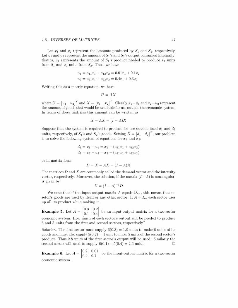
W. Leontief, who received a Nobel prize for economics in 1974, developeda method called input-output analysis in his study of economic systems andtheir component sectors. For example, a manufacturing plant might be thesystem and the various sectors could represent the different products made inthat plant. Or our system could be the entire economic complex of this countrywith some of the sectors being energy, agriculture, sports, manufacturing, etc.

To avoid unnecessary complications we describe this analysis for a two-sectoreconomic system. Thus, let S1 and S2 represent the two sectors involved. Weassume that part of each sector’s output is used within each of the sectors. Thatis, part of Sj ’s output is used by both S1 and S2 to produce their products. Forexample, suppose each unit of S1’s product requires 0.01 unit from S1 and 0.4unit from S2 while each unit of S2’s product requires 0.1 unit from S1 and 0.3unit from S2. We construct a matrix A using these data.

A = [aij ] =

[

0.01 0.10.4 0.3

]

is called the input-output matrix of the system. We need to make sure that theconvention used to construct A is understood. Thus,

a11 = 0.01 = amount of x1 needed to produce 1 unit of x1.




More generally,

ajk = amount of sector j’s output needed to produce 1 unit of sector

k’s goods.

Thus, the jth row of A tells us how much is needed from sector j by each ofthe other sectors, and the kth column of A tells how much the kth sector needsfrom each of the sectors.


Let x1 and x2 represent the amounts produced by S1 and S2, respectively.Let u1 and u2 represent the amount of S1’s and S2’s output consumed internally;that is, u1 represents the amount of S1’s product needed to produce x1 unitsfrom S1 and x2 units from S2. Thus, we have

u1 = a11x1 + a12x2 = 0.01x1 + 0.1x2

u2 = a21x1 + a22x2 = 0.4x1 + 0.3x2

Writing this as a matrix equation, we have

U = AX

where U =[

u1 u2]T

andX =[

x1 x2]T

. Clearly x1−u1 and x2−u2 representthe amount of goods that would be available for use outside the economic system.In terms of these matrices this amount can be written as

X −AX = (I −A)X

Suppose that the system is required to produce for use outside itself d1 and d2units, respectively, of S1’s and S2’s goods. Setting D =

[

d1 d2]T

, our problemis to solve the following system of equations for x1 and x2:

d1 = x1 − u1 = x1 − (a11x1 + a12x2)

d2 = x2 − u2 = x2 − (a21x1 + a22x2)

or in matrix formD = X − AX = (I −A)X

The matricesD andX are commonly called the demand vector and the intensityvector, respectively. Moreover, the solution, if the matrix (I−A) is nonsingular,is given by

X = (I −A)−1D

We note that if the input-output matrix A equals Onn, this means that nosetor’s goods are used by itself or any other sector. If A = In, each sector usesup all its product while making it.

Example 5. Let A =

[

0.3 0.20.1 0.4

]

be an input-output matrix for a two-sector

economic system. How much of each sector’s output will be needed to produce6 and 5 units from the first and second sectors, respectively?

Solution. The first sector must supply 6(0.3) = 1.8 units to make 6 units of itsgoods and must also supply 5(0.2) = 1 unit to make 5 units of the second sector’sproduct. Thus 2.8 units of the first sector’s output will be used. Similarly thesecond sector will need to supply 6(0.1) + 5(0.4) = 2.6 units. �

Example 6. Let A =

[

0.2 0.010.4 0.1

]

be the input-output matrix for a two-sector

economic system.


a. How much of the second sector’s product will be used in producing 6 unitsof the first sector’s goods and 3 units of the second sector’s goods?

Solution. In terms of the above notation, we are asked to find u2.

u2 = 6(0.4) + 3(0.1) = 2.4 + 0.3 = 2.7

Thus 2.7 units of the second sector’s output is needed to produce 6 and 3 unitsof the first and second sector’s products, respectively.

b. If D =

[

103

]

is a demand vector, how much should the economic system

produce in order to supply this demand from outside the system?

Solution. We need to find X =[

x1 x2]T

such that

(I −A)X = D =

[

103

]

Thus we should calculate (I − A)−1 if possible, for then X = (I −A)−1D.

I −A =

[

1 00 1

]

−[

0.2 0.010.4 0.1

]

=

[

0.8 −0.01−0.4 0.9

]

We easily see that (I −A) is invertible and its inverse is approximately equal to

(I −A)−1 ≈[

1.256 0.01390.5587 1.1173

]

Thus, since X = (I −A)−1[10, 3]T , we have

x1 ≈ 12.6017 x2 ≈ 8.9389 �

Problem Set 1.5

1. Determine which of the following matrices are invertible and then calculatetheir inverses

a.

[

2 31 4

]

b.

[

−2 −16 3

]

c.

[

1 −2 3−1 0 4

]

d.

−1 4 −10 2 11 0 3

2. Find the inverses of the following matrices if they exist.


a.

1 2 3 42 3 4 53 4 5 64 5 6 7

b.

1 0 1 00 1 0 11 1 0 00 1 1 0

c.

2 3 1 −13 −2 0 21 −1 −1 12 3 1 2

d.

6 −4 34 2 81 2 3

3. Suppose A is an n × n invertible matrix. If k is any positive integer, letA−k = (A−1)k. Show that ApAq = Ap+q where p and q are any integers,positive, negative, or zero.

4. Let A =

[

0.3 0.10 0.2

]

be an input-output matrix for some two-sector eco-

nomic system. Suppose 10 units of the second sector’s product are pro-duced.

a. how many units of the first sector’s product are needed by the secondsector?

b. How many units of the second sector’s product are needed by thesecond sector?

c. If the first sector produces exactly 10 units, what is the largest num-ber of units that sector 2 can make?

5. A biologist has been studying two different species of plants. Let xk andyk represent the population of each species in the kth year. Suppose shehas observed the following relationships between the populations:

xk+1 = 2xk + yk

yk+1 = 3xk + yk

a. Find a matrix A such that[

xk+1

yk+1

]

= A

[

xkyk

]

b. Show that[

xk+1

yk+1

]

= A2

[

xk−1

yk−1

]

c. Show that[

xkyk

]

= Ak

[

x0y0

]

for k = 1, 2, . . . .

d. If the population sizes in the third year are known, how can theinitial populations be determined; i.e.; what population size at timezero leads to the known populations?


e. Compute A3 and A−3.

Questions 6 and 7 refer to the input-output matrix A given below:

A =

0.1 0.2 0.10.2 0.1 0.40.0 0.2 0.3

6. How much of sector 2’s output is needed to produce 6 units of sector 3’sgoods?

7. How much of the first sector’s product is needed to produce 5, 8, and 9units of each of the first, second, and third sector’s products, respectively?

8. The matrix

1

2

1

30

1

2

1

2

1

31

4

1

5

1

2

is the input-output matrix for a three-sector economic system. How manyunits of the third sector’s product will be needed to simultaneously pro-duce 8 units from sector 1, 30 units from sector 2, and 14 units from sector3?

9. The matrix

1

2

1

20

1

20

1

2

01

2

1

3

is the input-output matrix for a three-sector economic system. If someoutside agency wants to purchase 2 units of sector 1’s product, 4 unitsof sector 2’s product, and 1 unit of the third sector’s, how much of thesecond product must be made?

10. Let E be the m × m elementary row matrix that corresponds to inter-changing row i and row j. Show that E−1 = E.

11. Let E be them×m elementary row matrix that corresponds to multiplyingrow i by c(c 6= 0). Find E−1.

12. Let A1, A2, . . . , Ak be a collection of n × n invertible matrices, k ≥ 3.Show (A1 . . . Ak)

−1 = (Ak)−1 . . . (A1)

−1.


13. An invertible matrix P such that each row has exactly one entry equal toone and all the other entries in this row equal to zero is called a permuta-tion matrix. There are exactly two 2× 2 permutation matrices, namely,

[

1 00 1

]

and

[

0 11 0

]

Notice that not only the rows of these matrices but also the columnscontain exactly one nonzero entry.

a. List all the 3 × 3 permutation matrices. There are 3! = 3(2) = 6 ofthem.

b. Show there are n! = n(n−1)(n−2) . . . (1) n×n permutation matrices.

c. If P is a permutation matrix, show that it can be obtained from theidentity matrix by a sequence of row interchanges.

14. Let P be an n × n permutation matrix (see problem 13). Show that PT

is also a permutation matrix and that PT = P−1.

15. Let D be any 2 × 2 diagonal matrix. Give a necessary and sufficientcondition on the diagonal entries so that D has an inverse. Compute theinverse of any such matrix.

16. Generalize problem 15 to n× n diagonal matrices.

17. Suppose A is a 3× 3 upper triangular matrix. Show that A has an inverseif and only if the diagonal elements of A are nonzero.

18. Suppose that A is an invertible matrix. Show that AT is also invertibleand that (AT )−1 = (A−1)T . (Hint: Use Theorem 1.5.)

19. Show that if A is symmetric and invertible, then A−1 is also symmetric.

20. Let A =

[

12 −1

−1 13

]

. Show that I −A is invertible and that all its entries

are positive.

Supplementary Problems

1. Define and give examples of each of the following:

a. The coefficient matrix of a nonhomogeneous system of equations

b. An elementary row matrix

c. An elementary row operation

d. A singular matrix

2. For each of the following find a system of equations for which the givenstatement is correct:


a. The solution set equals {(1,−2, 0)}.b. The solution set equals {(x1, x2) : x1 = 2}.c. The system has no solution.

3. Find the solution set for the system of equations:

6x1 − 4x3 = 1

2x1 + 3x2 = 2

+ x3 + x4 = −1

4. If A is a finite set of numbers, let av(A) denote the numerical averageof the numbers in A. Thus, if A = {1, 2,−4}, then av(A) = − 1

3 . LetA = {a, b, c} and B = {a, b, c, d}.

a. Show that, in general, it is not true that av(B) =[av(A) + d]/2.

b. Let A1 and A2 be two sets of numbers. Find a condition that willguarantee

av(A1 ∪ A2) =av(A1) + av(A2)

2

5. Find the solution sets for each of the following systems of equations:

a. x1 + x2 − x3 = 42x1 + 5x2 − 2x3 = 10

b. x1 − x2 + 2x3 = 1x1 + x2 + x3 = 2

3x1 + x2 + 4x3 = −4

c. x1 − x2 + 2x3 = 1x1 + x2 + x3 = 2

3x1 + x2 + 4x3 = 5

6. Suppose A =

[

a bc d

]

is invertible with A−1 =

[

e fg h

]

. Let B =

[

c da b

]

;

that is, B is obtained from A by a row interchange. Show that B−1 =[

f eh g

]

.

7. Let A be any n × n invertible matrix. Let B be the matrix obtainedby interchanging rows i and j of A. Show that B−1 equals the matrixobtained by interchanging columns i and j of A−1. (Hint: B = EA,where E is an elementary row matrix. What happens if we interchangetwo columns of A?)

8. Let M =

{[

a bc d

]

: ad− bc = 1

}

.


a. Show that M is closed under the operations of inversion and trans-position; that is, if A is in M , so are A−1 and AT .

b. If A and B are inM , must A+B be inM? What about their productAB?

9. The matrix A =

[

a bc d

]

is invertible if and only if there is a matrix

B =

[

x1 x2x3 x4

]

such that AB = I2 = BA. Write out the system of

four equations in the unknowns xj that arises from the matrix equationAB = I. Show that there is a solution if and only if ad−bc 6= 0. Assumingthis is true, solve for the unknowns xj ; then show that not only doesAB = I, but so too does BA.

10. Let B be any fixed n× n matrix. Let C(B) be the set of n× n matricesthat commute with B. That is, A is in C(B) if and only if AB = BA.Let A1 and A2 be any two matrices that are in C(B).

a. Show that aA1 + bA2 is in C(B) for any choice of constants a and b.

b. Show that A1A2 is in C(B).

11. Let A = [ajk] be an n× n invertible matrix. Suppose yj equalsn∑

k=1

ajkxk.

Show that xj =n∑

k=1

bjkyk, where [bjk] = A−1.

12. Let A be an n × n invertible matrix. Let Ej be the n × 1 matrix whoseonly nonzero entry is a 1 in the jth row. Show that the solution to theequation AX = Ej is the jth column of A−1.

13. Show that an n × n matrix A is invertible if and only if the equationAX = On1 has exactly one solution, namely, On1.

14. Let A be an 4 × 4 matrix that has been partitioned into four 2 × 2 sub-matrices. That is,

A =

[

A11 A12

A21 A22

]

where each Ajk is a 2 × 2 matrix. Let B = [Bjk] be a 4 × 4 matrixpartitioned in the same manner as A. Thus, each Bjk is also a 2 × 2matrix. Show that AB equals

[

A11B11 +A21B21 A11B12 +A12B22

A21B11 +A22B21 A21B12 +A22B22

]

15. Let A(t) = [ajk(t)] be an m×n matrix with its entries ajk(t) differentiablefunctions of t. Define A′(t) by A′(t) = [a′jk(t)]. Thus, if

A(t) =

[

cos t sin t− sin t cos t

]

then A′(t) =

[

− sin t cos t− cos t − sin t

]


Let A(t) and B(t) be two matrices whose entries are differentiable func-tions. Show that (A + B)′ = A′ + B′ and that (AB)′ = A′B + AB′

whenever it is possible to add or multiply the two given matrices.

16. Prove Theorem 1.5.

Documents

Matrices and Systems of Linear Equationsstecher/LinearAlgebraPdfFiles/...Chapter 1 Matrices and Systems of Linear Equations In Chapter 1 we discuss how to solve a system of linear