Matrix Compression using the Nystrom Method

Arik Nemtsov1 Amir Averbuch1 Alon Schclar2

1School of Computer Science

Tel Aviv University, Tel Aviv 69978

2School of Computer Science

The Academic College of Tel Aviv-Yaffo ,Tel Aviv, 61083

Abstract

The Nystrom method is routinely used for out-of-sample extension of kernel matrices.

We describe how this method can be applied to find the singular value decomposition

(SVD) of general matrices and the eigenvalue decomposition (EVD) of square matrices.

We take as an input a matrix M ∈ Rm×n, a user defined integer s ≤ min(m, n) and

AM ∈ Rs×s, a matrix sampled from columns and rows of M . These are used to construct

an approximate rank-s SVD of M in O(s2 (m + n)

)operations. If M is square, the

rank-s EVD can be similarly constructed in O(s2n)

operations. In this sense, AM is a

compressed version of M .

We discuss theoretical considerations for the choice of AM and how it relates to the

approximation error. Finally, we propose an algorithm that selects a good initial sample

for a pivoted version of M . The algorithm relies on a previously computed approximate

rank-s decomposition of M , termed Mdecomp. We show that ||Mdecomp − M ||2 is related

to the Nystrom approximation error when the selected sample is employed. Then, the

user can choose a more computationally expensive algorithm for computing Mdecomp when

higher accuracy is required.

We present experimental results that evaluate our sample selection algorithm for gen-

eral matrices and kernel matrices. The algorithm is shown to work well for matrices whose

spectra exhibit fast decay.

Key words: {SVD, EVD, Nystro, out-of-sample extension}2000 MSC: {65F15, 65F30, 65F50}

1

1 Introduction

Low rank approximation of linear operators is an important problem in the areas of scien-

tific computing and statistical analysis. Approximation reduces storage requirements for large

datasets and improves the runtime complexity of algorithms operating on the matrix. When

the matrix contains affinities between elements, low rank approximation can be used to reduce

the dimension of the original problem ([25, 26, 28]) and to eliminate statistical noise ([27]).

Our approach involves the choice of a small sub-sample from the matrix, followed by the

application of the Nystrom method for out-of-sample extension. The Nystrom method ([1]),

which originates from the field of integral equations, is a way of discretizing an integral equation

using a simple quadrature rule. When given an eigenfunction problem of the form

λf(x) =

∫ b

a

M (x, y) f (y) dy,

the Nystrom method employs a set of s sample points y1, . . . , ys that approximate f(x) as

λf (x) � b − a

s

s∑j=1

M (x, yj) f (yj).

In recent years, the Nystrom method has gained widespread use in the field of spectral clus-

tering. It was first popularized by [16] for sparsifying kernel matrices by approximating their

entries. The matrix completion approach of [2] also enables the approximation of eigenvectors.

It was now possible to use the Nystrom method in order to speed up algorithms that require the

spectrum of a kernel matrix. Over time, Nystrom based out-of-sample extensions have been de-

veloped for a wide range of spectral methods, including Normalized-Cut ([17, 18]), Geometric

Harmonics ([19]) and others ([20]).

In this paper, we present two extensions of the matrix completion approach of [2]. These allow

us to form the SVD and EVD of a general matrix through the application of the Nystrom

method on a previously chosen sample.

In addition, we present a novel algorithm for selecting the initial sample to be used with the

Nystrom method. Our algorithm is applicable to general matrices whereas previous methods

focused on kernel matrices. The algorithm uses a pre-existing low-rank decomposition of the

input matrix. We show that our sample choice reduces the Nystrom approximation error.

The paper is organized as follows: Section 2 describes the basic Nystrom matrix form and the

methods of [2] for finding the EVD of a Nystrom approximated symmetric matrix. Section 3

outlines a Nystrom-like method for out-of-sample extension of general matrices, starting with

2

the SVD of a sample matrix. In section 4 we describe procedures that explicitly generate the

canonical SVD and EVD forms for general matrices. Section 5 introduces the problem of sample

choice and presents results that bound the accuracy of the algorithm in section 6. Section 6

presents our sample selection algorithm and analyzes its complexity. Experimental results on

general and kernel matrices are presented in section 7.

2 Preliminaries

2.1 Square Nystrom Matrix Form

Let M ∈ Rn×n be a square matrix. We assume that the M can be decomposed as

M =

⎡⎣ AM BM

FM CM

⎤⎦ (2.1)

where AM ∈ Rs×s, BM ∈ R

s×(n−s), FM ∈ R(n−s)×s and CM ∈ R

(n−s)×(n−s). The matrix AM is

designated to be our sample matrix. The size of our sample is s, which is the size of AM .

Let UΛU−1 be the eigen-decomposition of AM , where U ∈ Rs×s is the eigenvectors matrix

and Λ ∈ Rs×s is the eigenvalues matrix. Let ui ∈ R

s be the column eigenvector belonging to

eigenvalue λi. We aim to extend the column eigenvector (the discrete form of an eigenfunction)

to the rest of M . Let ui =[

ui ui

]T∈ R

n be the extended eigenvector, where ui ∈ Rn−s is

the extended part. By applying the Nystrom method to ui, we get the following form for the

kth coordinate in ui:

λiuik � b − a

s

s∑j=1

Mkj · uij. (2.2)

By setting [a, b] = [0, 1] and presenting Eq. (2.2) in matrix product form we obtain

λiui =

1

sFM · ui. (2.3)

This can be done for all the eigenvalues {λi}si=1 of AM . Denote U =

[u1 . . . us

]∈ R

(n−s)×s.

By placing all expressions of the form Eq. (2.3) side by side we have UΛ = FMU . Assuming

the matrix AM has non-zero eigenvalues (we will return to this assumption later), we obtain:

U = FMUΛ−1. (2.4)

Analogically, we can derive a matrix representation for extending the left eigenvectors of M ,

denoted as V ∈ Rs×n−s:

V = Λ−1U−1BM . (2.5)

3

Combining Eqs. (2.4) and (2.5) with the eigenvectors of AM yields the full left and right

approximated eigenvectors:

U =

⎡⎣ U

FMUΛ−1

⎤⎦ , V =

[U−1 Λ−1U−1BM

]. (2.6)

The explicit “Nystrom” representation of M becomes:

M = UΛV =

⎡⎣ U

FMUΛ−1

⎤⎦Λ

[U−1 Λ−1U−1BM

]=

⎡⎣ AM BM

FM FMA+MBM

⎤⎦ =

⎡⎣ AM

FM

⎤⎦A+

M

[AM BM

] (2.7)

where A+M denotes the pseudo-inverse of AM .

Equation (2.7) shows that the Nystrom extension does not modify AM , BM and FM , and that

it approximates CM by FMA+MBM .

2.2 Decomposition of Symmetric Matrices

The algorithm given in [2] is a commonly used method for SVD approximation of symmetric

matrices. For a given matrix, it computes the SVD of its Nystrom approximated form. The SVD

and EVD of a symmetric matrix coincide, therefore the SVD approximates both simultaneously.

We describe the method of [2] in section 2.2.2.

2.2.1 Symmetric Nystrom Matrix Form

When M is symmetric, the matrix M has the decomposition

M =

⎡⎣ AM BM

BTM CM

⎤⎦ (2.8)

where AM ∈ Rs×s, BM ∈ R

s×(n−s) and CM ∈ R(n−s)×(n−s). We replace FM in Eq. (2.1) with

BTM .

By using reasoning similar to section 2.1, we can express the right and left approximated

eigenvectors as:

U =

⎡⎣ U

BTMUΛ−1

⎤⎦ , V =

[U−1 Λ−1U−1BM

]. (2.9)

4

The explicit “Nystrom” representation of M becomes:

M = UΛV =

⎡⎣ U

BTMUΛ−1

⎤⎦Λ

[U−1 Λ−1U−1BM

]=

⎡⎣ AM BM

BTM BT

MA+MBM

⎤⎦ =

⎡⎣ AM

BTM

⎤⎦A+

M

[AM BM

].

(2.10)

2.2.2 Construction of SVD for Symmetric M

Our goal is to find the s leading eigenvalues and eigenvectors of M without explicitly forming

the entire matrix.

We begin with the decomposition of M as in Eq. (2.8). The approximation technique in [2] uses

the standard Nystrom method in Eq. (2.9) to obtain U . Then, the algorithm forms the matrix

Z = UΛ1/2 such that M = ZZT = UΛUT . The symmetric s × s matrix ZT Z is diagonalized

as FΣF T . The eigenvectors of M are given by Uo = ZFΣ−1/2 and the eigenvalues are given by

Σ. To qualify for use in the SVD, Uo and Σ must meet the following requirements:

1. The columns of Uo must be orthogonal. Namely, UTo Uo = I.

2. The SVD form of Uo and Σ must form M . Formally, M = UoΣUTo .

The following identities can be readily verified using our expressions for Uo and Σ:

1. Bi-orthogonality: UTo Uo = Σ−1/2F T ZT ZFΣ−1/2 = Σ−1/2F T

(FΣF T

)FΣ−1/2 = I;

2. SVD form: UoΣUTo = ZFΣ−1/2 · Σ · Σ−1/2F T ZT = ZZT = M.

The computational complexity of the algorithm is O (s2n), where s is the sample size and n is

the number of rows and columns of M . The bottleneck is in the computation of the matrix

product ZT Z.

2.2.3 A Single-Step Solution for the SVD of M

The “one-shot” solution in [2] assumes that AM has a square root matrix A1/2M . This assumption

is true if the matrix is positive definite. Otherwise, it imposes some limitations on AM . These

will be discussed later.

Let A−1/2M be the pseudo-inverse of the square root matrix of AM . Denote GT = A

−1/2M

[AM BM

].

From this definition we have M = GGT . The matrix S ∈ Rs×s was defined in [2], where

5

S = GT G = AM + A−1/2M BMBT

MA−1/2M . S is fully decomposed as USΛSUT

S . The orthogonal

eigenvectors of M are formed as Uo = GUSΛ−1/2S and the eigenvalues are given in ΛS.

The following required identities, as in section 2.2.2, can again be verified as follows:

1. Bi-orthogonality:

UTo Uo = Λ

−1/2S UT

S GT GUSΛ−1/2S = Λ

−1/2S UT

S SUSΛ−1/2S = Λ

−1/2S UT

S · USΛSUTS · USΛ

−1/2S = I.

2. SVD form: UoΛSUTo = GUSΛ

−1/2S · ΛS · Λ−1/2

S UTS GT = GGT = M.

The computational complexity remains the same (the bottleneck of the algorithm is the for-

mation of BMBTM). However this version is numerically more accurate. According to [2], the

extra calculations in the general method of solution lead to an increase in the loss of significant

digits.

3 Nystrom-like SVD approximation

The SVD of a matrix can also be approximated via the basic quadrature technique of the

Nystrom method. In this case, we do not require an eigen-decomposition. Therefore, M does

not necessarily have to be square. Let M ∈ Rm×n be a matrix with the decomposition given in

Eq. (2.1). We begin with the SVD form AM = UΛH where U,H ∈ Rs×s are unitary matrices

and Λ ∈ Rs×s is diagonal. We assume that zero is not a singular value of AM . Accordingly, U

can be formulated as:

U = AMHΛ−1. (3.1)

Let ui, hi ∈ Rs be the ith columns in U and H, respectively. Let ui = {ui

l}sl=1 be the partition

of ui into elements. By using Eq. (3.1), each element uil can be presented as the sum ui

l =

1λi

∑nj=1 Mlj · hi

j.

We can use the entries of FM as interpolation weights for extending the singular vector ui

to the kth row of M , where s + 1 ≤ k ≤ n. Let ui = {uik−s}n

k=s+1 ∈ Rn−s be a column

vector that contains all the approximated entries. Each element uik−s will be calculated as

uik−s = 1

λi

∑nj=1 Mkj · hi

j. Therefore, the matrix form of ui becomes ui = 1λi

FM · hi.

Putting together all the ui’s as U =[

u1 u2 . . . us

]∈ R

n−s×s, we get U = FMHΛ−1.

The basic SVD equation of AM can also be written as H = ATMUΛ−1. We approximate the

right singular vectors of the out-of-sample columns by employing a symmetric argument. We

obtain H = BTMUΛ−1.

6

The full approximations of the left and right singular vectors of M , denoted by U and H,

respectively, are

U =

⎡⎣ U

FMHΛ−1

⎤⎦ , H =

⎡⎣ H

BTMUΛ−1

⎤⎦ . (3.2)

The explicit “Nystrom” form of M becomes

M = UΛHT =

⎡⎣ U

FMHΛ−1

⎤⎦Λ

[HT Λ−1UT BM

]=

⎡⎣ AM BM

FM FMA+MBM

⎤⎦ =

⎡⎣ AM

FM

⎤⎦A+

M

[AM BM

] (3.3)

where A+M denotes the pseudo-inverse of AM . M does not modify AM , BM and FM but approx-

imates CM by FMA+MBM . Note that the Nystrom matrix form of the SVD is similar to Eq.

(2.7), which is the Nystrom form of the EVD matrix.

4 Decomposition of General Matrices

We will refer to a decomposition of M given in Eq. (2.1) with the corresponding decomposition

into AM , BM , FM and CM . M denotes the approximated Nystrom matrix.

This section presents procedures for explicit orthogonalization of the singular-vectors and eigen-

vectors of M . Starting with M in the form of Eqs. (2.7) and (3.3), we find its canonical SVD

and EVD form, respectively. Constructing these representations takes time and space that are

linear in the dimensions of M .

4.1 Construction of EVD for M

Let M be a square matrix. We will approximate the eigenvalue decomposition of M without

explicitly forming M .

We begin with a matrix M that is partitioned as in Eq. (2.1). By explicitly employing the

Nystrom method, we construct U and V as defined in Eq. (2.6). Then, we proceed by defining

the matrices GU = UΛ1/2 and GV = Λ1/2V . We directly compute the EVD of GV GU as FΣF−1.

The eigenvalues of M are given by Σ and the right and left eigenvectors are Uo = GUFΣ−1/2

and Vo = Σ−1/2F−1GV , respectively.

The left and right eigenvectors are mutually orthogonal since

VoUo = Σ−1/2F−1GV · GUFΣ−1/2 = Σ−1/2F−1 · FΣF−1 · FΣ−1/2 = I.

7

The EVD form of Uo, Vo and Σ gives M , as we see from

UoΣVo = GUFΣ−1/2 · Σ · Σ−1/2F−1GV = GUGV = UΛ1/2 · Λ1/2V = M.

These two properties qualify UoΣVo as the EVD of M .

When M is symmetric, the matrix GV is simply GTU . By using the terminology in section

2.2.2, we denote GV = Z and the matrix GV GU is transformed into ZZT . From here on the

method of solution in section 2.2.2 coincides with the current section. Hence, this form of EVD

approximation generalizes the symmetric case.

The computational complexity is O(s2n), where s is the sample size (the size of AM) and n is

the size of M . The computational bottleneck is in the formation of GV GU .

4.1.1 A Single-Step Solution for the EVD for M

This solution method assumes that AM has a square root matrix A1/2M . From this assumption,

we can modify the algorithm in section 4.1 to construct the EVD of M with fewer steps.

We define the matrices GU and GV to be

GU =

⎡⎣ AM

FM

⎤⎦A

−1/2M , GV = A

−1/2M

[AM BM

].

We proceed to explicitly compute the eigen-decomposition of GV GU ∈ Rs×s as GV GU =

FΣF−1. The eigenvalues of M are given by Σ and the right and left eigenvectors of M are

formed by Uo = GUFΣ−1/2 and Vo = Σ−1/2F−1GV , respectively. Again, we can verify the

eigenvectors are mutually orthogonal:

VoUo = Σ−1/2F−1GV ·GUFΣ−1/2 = Σ−1/2F−1 ·GV GU ·FΣ−1/2 = Σ−1/2F−1 ·FΣF−1 ·FΣ−1/2 = I,

and the matrices Uo, Vo and ΛS form M as

UoΛSVo = GUFΣ−1/2 · Σ · Σ−1/2F−1GV = GUGV =

⎡⎣ AM

FM

⎤⎦A

−1/2M · A−1/2

M

[AM BM

]= M.

The reduction to the symmetric case is straightforward here as well. We have GV = GTU when

M is symmetric. By using the terms of section 2.2.3, we have GTU = GV = G. The expression

GV GU turns into GT G. After that point the methods of solution coincide.

Again, the algorithm takes O(s2n) operations due to the need to calculate GV GU . Compared

to the solution given in section 4.1, the single-step solution performs fewer matrix operations.

Therefore, it achieves better numerical accuracy.

8

4.2 Construction of SVD for M

Let M be a general m×n matrix with the decomposition in Eq. (2.1). Given an initial sample

AM , we present an algorithm that efficiently computes the SVD of M (defined by Eq. (2.7)).

We explicitly compute the SVD of AM and use the technique outlined in section 3 to obtain U

and H as in Eq. (3.2). We form the matrices ZU = UΛ1/2 and ZH = HΛ1/2. We proceed by

forming the symmetric s × s matrices ZTU ZU and ZT

HZH and compute their SVD as ZTU ZU =

FUΣUF TU and ZT

HZH = FHΣHF TH , respectively. The next stage derives an SVD form for the

s × s matrix D = Σ1/2U F T

U FHΣ1/2H . This is given explicitly by computing D = UDΛDHT

D. The

singular values of M are given in ΛD and the leading left and right singular vectors of M are

Uo = ZUFUΣ−1/2U UD and Ho = ZHFHΣ

−1/2H HD, respectively. The columns of Uo and Ho are

orthogonal since

UTo Uo = UT

DΣ−1/2U F T

U ZTU · ZUFUΣ

−1/2U UD = UT

DΣ−1/2U F T

U · FUΣUF TU · FUΣ

−1/2U UD = UT

DUD = I,

HTo Ho = HT

DΣ−1/2H F T

HZTH ·ZHFHΣ

−1/2H HD = HT

DΣ−1/2H F T

H ·FHΣHF TH ·FHΣ

−1/2H HD = HT

DHD = I.

The SVD of M is formed by using Uo, Ho and VD

UoΛDoHTo = ZUFUΣ

−1/2U UD · ΛD · HT

DΣ−1/2H F T

HZTH = ZUFUΣ

−1/2U · D · Σ−1/2

H F THZT

H =

= ZUFUΣ−1/2U · Σ1/2

U F TU FHΣ

1/2H · Σ−1/2

H F THZT

H = ZUZTH = UΛ1/2 · Λ1/2HT = M.

When M is symmetric, this solution method coincides with the method in section 2.2.2. The

matrices ZU and ZH correspond to Z in section 2.2.2. The matrix D becomes the diagonal ma-

trix Σ of the symmetric case. The computational complexity of the procedure is O (s2 (m + n)).

The bottleneck is the computation of ZTU ZU and ZT

HZH .

4.2.1 A Single-Step Solution for the SVD of M

This solution method assumes that AM has a square root matrix A1/2M . Similar to section 4.1.1,

this assumption allows us to modify the algorithm of the general case to achieve the same result

in fewer steps.

Let A−1/2M be the pseudo-inverse of the square root matrix of AM . We begin by forming the

matrices GU and GH such that

GU =

⎡⎣ AM

FM

⎤⎦A

−1/2M , GH =

(A

−1/2M

[AM BM

])T

.

9

The symmetric matrices GTUGU and GT

HGH are diagonalized by GTUGU = FUΣUF T

U and GTHGH =

FHΣHF TH . From these parts we form D = Σ

1/2U F T

U FHΣ1/2H which is explicitly diagonalized as

D = UDΛDHTD. The singular values of M are given by ΛD and the left and right singular

vectors are given by Uo = GUFUΣ−1/2U UD and Ho = GHFHΣ

−1/2H HD, respectively.

As in section 4.2, we can verify the identities that make this decomposition a valid SVD. The

singular vectors are orthogonal:

UTo Uo = UT

DΣ−1/2U F T

U GTU · GUFUΣ

−1/2U UD = UT

DΣ−1/2U F T

U · FUΣUF TU · FUΣ

−1/2U UD = UT

DUD = I,

HTo Ho = HT

DΣ−1/2H F T

HGTH ·GHFHΣ

−1/2H HD = HT

DΣ−1/2H F T

H ·FHΣHF TH ·FHΣ

−1/2H HD = HT

DHD = I.

The SVD is formed by Uo, Ho and ΛD:

UoΛDHTo = GUFUΣ

−1/2U UD · ΛD · HT

DΣ−1/2H F T

HGTH = GUFUΣ

−1/2U · D · Σ−1/2

H F THGT

H =

= GUFUΣ−1/2U · Σ1/2

U F TU FHΣ

1/2H · Σ−1/2

H F THGT

H = GUGTH =

⎡⎣ AM

FM

⎤⎦A

−1/2M · A−1/2

M

[AM BM

]= M.

If M is symmetric, this method reduces to the single-step solution described in section 2.2.3.

The matrices GU and GH correspond to G in the symmetric case. The matrix D becomes ΛS.

The computational complexity of the procedure remains O (s2 (m + n)). The computational

bottleneck of the algorithm is in the formation of GTUGU .

4.3 Prerequisite for the Single-Step methods

The single-step methods, described in sections 2.2.3, 4.1.1 and 4.2.1, require that AM have a

square root matrix.

When a matrix is positive semi-definite, a square root can be found via the Cholesky factor-

ization algorithm ([5] chapter 4.2.3). But positive-definiteness is not a necessary prerequisite.

For example, the square root of a diagonalizable matrix can be found via its diagonalization. If

AM = UΛU−1, then, A1/2M = UΛ1/2U−1. In this case, the matrix does not need to be invertible.

It can be shown that under a complex realm, every non-singular matrix has a square root. An

algorithm for calculating the square root for a given non-singular matrix is given in [15]. This

suggests a way of assuring the existence of a square root matrix. We can make AM non-singular,

or equivalently, a full rank matrix.

The rank of AM will also have a role in bounding the approximation error of the Nystrom

procedure. This will be elaborated in section 5.3.

10

5 Choice of Sub-Sample

The choice of initial sample for performing the Nystrom extension is an important part in the

approximation procedure. The sample matrix AM is determined by permutation of the rows

and columns of M (as given in Eq. (2.1)). Our goal is to choose a (possibly constrained)

permutation of M such that the resulting matrix can be approximated more accurately by the

Nystrom method. Here accuracy is measured by L2 distance between the pivoted version of M

and the Nystrom approximated version. This notion is made precise in section 5.3.

We allow for complete pivoting in the choice of a permutation for M . This means that both

columns and rows can be independently permuted. This kind of pivoting does not generally

preserve the eigenvalues and eigenvectors of the matrix. However, the singular values of the

matrix remain unchanged and the singular vectors are permuted. Formally, let Er and Ec be the

row and column permutation matrices, respectively. Using the SVD of M , the pivoted matrix

is decomposed as ErMEc = ErUΣV T Ec = (ErU) Σ(V T Ec

). Row and column permutations

leave U and V T unitary. Therefore (ErU) Σ(V T Ec

)is the SVD of ErMEc. The singular vectors

of M can be easily regenerated by permuting the left and right singular vectors of ErMEc by

E−1r and E−1

c respectively.

Section 5.3 shows the choice of AM determines the Nystrom approximation error. Hence, the

problem of choosing a sample is equivalent to choosing the rows and columns of M whose

intersection forms AM . Therefore, it makes sense to use the size s of AM as our sample size.

This size largely determines the time and space complexity of the presented approximation

procedures. The complexities are O (s2 (m + n)) and O (s (m + n)), respectively.

5.1 Related Work on Sub-Sample Selection

Previous works on sub-sample selection focused on kernel matrices. These were done for sym-

metric matrices where the entries represent affinities. In these settings, we can use a single

permutation for the columns and rows without changing the original meaning of the matrix.

This pivoting variant is called symmetric pivoting. Sample selection algorithms for kernel ma-

trices try to find a permutation matrix Ep such that ETp MEp is most accurately approximated

by the Nystrom method.

The simplest sample selection method is based on random sampling. It works well for dense

image data ([2]). Random sampling is also used in [23] while employing a greedy criterion that

helps to determine the quality of the sample. A different greedy approach for sample selection is

11

used in [21], where a new point is added to the sample based on its distance from a constrained

linear combination of previously selected points.

In [22], the k -means clustering algorithm is used for selecting the sub-sample. The k -means

cluster centers are shown to minimize an error criterion related to the Nystrom approximation

error. Finally, Incomplete Cholesky Decomposition (ICD) ([12]) employs the pivoted Choleksy

algorithm and uses a greedy stopping criterion to determine the required sample size for a given

approximation accuracy.

The Cholesky decomposition of a matrix factors it into ZT Z, where Z is an upper triangular

matrix. Initially, Z = 0. The ICD algorithm applies the Cholesky decomposition to M while

symmetrically pivoting the columns and rows of M according to a greedy criterion. The al-

gorithm has an outer loop that scans the columns of M according to a pivoting order. The

results for each column determine the next column to scan. This loop is terminated early after

s columns were scanned by using a heuristic on the trace of the residual ZT Z − M . This

algorithm ([12]) approximates M . This is equivalent to a Nystrom approximation where the

initial sample is taken as the intersection of the pivoted columns and rows.

When M is a Gram matrix, it can be expressed as the product of two matrices. Let M be

decomposed into M = XT X where X ∈ Rn×n. The special properties of M were exploited

differently in [13]. Specifically, the fact that Mii is the norm of the column Xi is used. A

non-Gram matrix requires O(n2) additional operations to compute XTi Xi, which is impractical

for large matrices. Once the norms of the columns in X are known, a method similar to [6] is

used to choose a good column sample from X. The intersection in M of the pivoted columns

and the corresponding rows is a good choice for AM . The Nystrom procedure is then performed

similarly to what was described in section 2.2.2. The runtime complexity of the algorithm in

[13] is O(n).

5.2 Preliminaries

Definition 5.1. Approximate ‘thin’ Matrix Decomposition. Given a matrix M ∈ Rm×n.

A ”thin” matrix decomposition is an approximation of the form M = GS where G ∈ Rm×k,

S ∈ Rk×n and k ≤ min(m,n).

This form effectively approximates M using a rank-k matrix product. A good example for such

an approximation is the truncated rank-k SVD. It approximates a m×n matrix as UΛV T , where

U ∈ Rm×k, Λ ∈ R

k×k and V ∈ Rn×k. When this decomposition is employed, we can choose,

12

for example, G = U, S = ΛV T . Many algorithms ([6, 9, 10, 11]) exist for approximating the

rank-k SVD with a runtime close to O(mn).

Truncated SVD is a popular choice, but it is by no means the only one. Other examples include

truncated pivoted QR ([7]) or the interpolative decomposition (ID) as outlined in [8].

Definition 5.2. Numerical Rank. A matrix A has numerical rank r with respect to a

threshold ε if σr+1(A) is the first singular value such that

σ1 (A)

σr+1(A)> ε.

This definition generalizes the L2 condition number (κ2 (A)), since it also applies to non-

invertible and non-square matrices.

Definition 5.3. Rank Revealing QR Decomposition (RRQR). Let A ∈ Rm×n be a

matrix and let k be a user defined threshold. A RRQR algorithm finds a permutation matrix E

such that AE has a QR decomposition with special properties. Formally, we write AE = QR

such that Q is an orthogonal matrix and R is upper triangular. Let R have the following

decomposition:

R =

⎡⎣ R11 R12

0 R22

⎤⎦ (5.1)

where R11 ∈ Rk×k, R12 ∈ R

k×(n−k) and R22 ∈ R(m−k)×(n−k). Let p (k, n) be a fixed non-negative

function bounded by a low degree polynomial in k and n. A RRQR algorithm tries to permute

the columns of A such that

σk (R11) ≥ σk (A)

p(k, n), σ1 (R22) ≤ σk+1 (A) · p(k, n).

An overview on this topic is given in [3].

The relation between A and R can shed some light on the rank-revealing properties of RRQR.

Let AE =[

A1 A2

]be a partitioning of AE such that A1 contains the first k columns. The

RRQR decomposition is rank-revealing in the sense that it tries to put a set of k maximally

independent columns of A into A1. We formalize this statement with Lemma 5.4.

Lemma 5.4. Assume that the RRQR algorithm found a pivoting of A such that σk (R11) ≥σk (A)/β, where β ≥ 1. If A has numerical rank of at least k with respect to the threshold ε,

then, the numerical rank of A1 (the first k columns of AE) is k with respect to the threshold

β · ε.

13

Proof. The RRQR algorithm yields A1 = Q[

R11 0]T

. Since Q is orthogonal, it does not

modify singular values. Therefore, we have σk (A1) = σk

[R11 0

]T= σk (R11). By combining

the above with our assumption on the RRQR algorithm, we get

β · σk (A1) ≥ σk (A) . (5.2)

The interlacing property of singular values (Corollary 8.6.3 in [5]) gives us

σ1 (A) ≥ σ1 (A1) . (5.3)

By employing definition 5.2 for A and incorporating Eqs. (5.2) and (5.3), we get

ε ≥ σ1 (A)

σk(A)≥ σ1 (A1)

σk(A)≥ σ1 (A1)

β · σk (A1).

By rearranging terms, we getσ1 (A1)

σk (A1)≤ β · ε.

Therefore the numerical rank of A1 is at least k with respect to the threshold β · ε. Since A1

has only k columns, it has precisely this rank.

5.3 Analysis of Nystrom Error

Let M be a matrix with the decomposition given by Eq. (2.1). This partitioning corresponds

to sampling s columns and rows from M to form the matrix AM . Our error analysis depends

on an approximate decomposition of M into a product of two ‘thin’ matrices. Let M � GS be

a decomposition of M where G ∈ Rm×s and S ∈ R

s×n. The approximation error of M by GS

is denoted by es. Formally, ||M − GS||2 ≤ es. Let G =[

GA GB

]Tbe a row partitioning of

G where GA ∈ Rs×r and GB ∈ R

(m−s)×r. Let S = [ SA SB ] be a column partitioning of S

where SA ∈ Rr×s, SB ∈ R

r×(n−s). This notation yields the following forms for the sub-matrices

of M :

AM � GASA, BM � GASB, FM � GBSA, CM � GBSB. (5.4)

where AM , BM , FM and CM were defined in Eq. 2.1.

Lemma 5.5. (based on Corollary 8.6.2 in [5]) If A and A + E are in Rm×n then for

k ≤ min (m,n) we have |σk (A + E) − σk (A)| ≤ σ1 (E) = ||E||2.

Proof. Corollary 8.6.2 in [5] states the same lemma with the requirement m ≥ n. If m < n,

we can use the original version of the lemma to get∣∣σk

(AT + ET

)− σk

(AT)∣∣ ≤ ∣∣∣∣ET

∣∣∣∣2.

Transposition neither modifies the singular values nor the norm of a matrix.

14

Theorem 5.6. Assuming that

1. σs (G) σs (S) = σs (GS) /γ for some constant γ ≥ 1;

2. The matrices GA and SA are non-singular;

3. σs(GA) ≥ σs(G)/β and σs(SA) ≥ σs(S)/β for some constant β ≥ 1;

4. es < (σs (M) − es) /β2γ, where es is the error given by the rank-s approximation of M by

GS.

Then, AM is non-singular.

Proof. Lemma 5.5 yields |σs (M) − σs (GS)| ≤ ||M − GS||2 = es, or

σs (M) − es ≤ σs (GS) . (5.5)

From assumptions 1 and 3 we obtain

σs (GS) /β2γ ≤ σs (G) σs (S) /β2 ≤ σs (GA) σs (SA) . (5.6)

GA and SA are s × s non-singular matrices. Thus, we obtain

σs (GA) σs (SA) =1∣∣∣∣G−1

A

∣∣∣∣ ∣∣∣∣S−1A

∣∣∣∣ ≤ 1∣∣∣∣S−1A G−1

A

∣∣∣∣ =1∣∣∣∣(GASA)−1

∣∣∣∣ = σs (GASA) . (5.7)

By combining Eqs. (5.5), (5.6) and (5.7) we get

(σs (M) − es) /β2γ ≤ σs (GASA) . (5.8)

AM and GASA are the top left s × s corners of M and GS, respectively. Hence, we can write

||AM − GASA||2 ≤ ||M − GS||2 = es. By combining this expression with Eq. (5.8) and using

assumption 4, we have ||AM − GASA||2 ≤ σs (GASA). Equivalently,

||AM − GASA||2||GASA||2

<1

κ (GASA). (5.9)

The matrix GASA is non-singular since it is the product of the non-singular matrices GA and

SA. Equation 2.7.6 in [5] states that for any matrix A and perturbation matrix ΔA we have

1

κ2 (A)= min

A+ΔA singular

||ΔA||2||A||2

.

This equation in effect gauges the minimal L2 distance from A to a singular matrix. By setting

GASA = A in Eq. (5.9) we conclude that AM is non-singular.

15

Assumption 1 can be verified for different types of rank-s approximations of M . For the

approximated SVD we have Corollary 5.7.

Corollary 5.7. When the approximated SVD is used to form GS, we have γ = 1 (where γ is

defined by assumption 1 in Theorem 5.6).

Proof. Let M � UΣV T be the approximated SVD of M . We can choose G = UΣ and S = V T .

From the properties of the SVD, we have σs (G) = σs (UΣ) = Σss = σs (GS) and σs (S) = 1. It

follows that σs (G) σs (S) = σs (GS).

Similarly, the β in assumption 3 depends on the algorithm that is used to pick GA and SA

from within G and S, respectively. When a state-of-the-art RRQR algorithm is used, we derive

Corollary 5.8.

Corollary 5.8. When the RRQR version given in Algorithm 1 in [4] is used to choose GA and

SA, we have β ≤√s (min (m,n) − s) + 1 , where β is defined by assumption 3 in Theorem 5.6.

Proof. Let A ∈ Rn×k be a matrix where k ≤ n and a let A =

[A1 A2

]be a partition of A

where A1 ∈ Rk×k. The concept of local μ-maximum volume was used in [4] to find a pivoting

scheme such that σmin (A1) is bounded from below. Formally, Lemma 3.5 in [4] states that when

A1 is a local μ-maximum volume in A, we have σmin (A1) ≥ σk (A) /√

k (n − k) μ2 + 1. μ is

a user-controlled parameter that has negligible effect in this bound. For instance, [4] suggests

setting μ = 1 + u, where u is the machine precision. Therefore, we omit μ in subsequent

references of this bound.

Algorithm 1 in [4] describes how a local μ-maximum volume can be found for a given matrix

A. This algorithm can be applied to the choice of GA and STA from the rows of G and ST ,

respectively. It follows from Lemma 3.5 in [4] that σs (GA) ≥ σs (G) /√

s (m − s) + 1 and

σs (SA) = σs

(ST

A

) ≥ σs

(ST)/√

s (n − s) + 1 = σs (S) /√

s (n − s) + 1. The definition of β

yields the required expression.

Later the RRQR algorithm will be used to select GTA and SA as columns from GT and S,

respectively. This is equivalent to choosing rows from G and ST . The latter form was used for

compatibility with the notation of [4].

Theorem 5.6 states that if our rank-s approximation of M is sufficiently accurate and our

RRQR algorithm managed to pick s non-singular columns from GT and S, then our sample

matrix AM is non-singular.

16

We bring a few definitions in order to bound the error of the Nystrom approximation procedure.

We will decompose the matrix M into a sum of two matrices: Mlg that contains the energy of

the top s singular values and Msm that contains the residual. If Mlg and Msm are given in SVD

outer product form, then we have Mlg =∑s

i=1 σiuivi and Msm =∑min(m,n)

i=s+1 σiuivi, respectively.

Based on this decomposition, we define the following decompositions of Mlg and Msm:

M = Mlg + Msm =

⎡⎣ AM BM

FM CM

⎤⎦ =

⎡⎣ Alg Blg

Flg Clg

⎤⎦+

⎡⎣ Asm Bsm

Fsm Csm

⎤⎦ . (5.10)

Lemma 5.9. If all the assumptions of Theorem 5.6 hold and if we have

σs+1 (M) <σs (M) − es

β2γ− es (5.11)

(where es is defined by assumption 4 in Theorem 5.6), then Alg is non-singular.

Proof. We employ Lemma 5.5 to bound |σs (AM) − σs (GASA)|. Formally, we have

|σs (AM) − σs (GASA)| ≤ ||AM − GASA||2 ≤ ||M − GS||2 = es.

By rearranging terms, we obtain σs (GASA) − es ≤ σs (AM). Combining this expression with

Eq. (5.8) from the proof of Theorem 5.6 yields

σs (M) − es

β2γ− es ≤ σs (AM) . (5.12)

The quantity ||AM − Alg||2 can be bounded by ||AM − Alg||2 ≤ ||M − Mlg||2 = σs+1 (M).

Combining the above with Eqs. (5.11) and (5.12) yields

||AM − Alg||2 ≤ σs+1 (M) <σs (M) − es

β2γ− es ≤ σs (AM) .

The terms are rearranged to get

||AM − Alg||2 / ||AM ||2 < 1/κ (AM) , (5.13)

where κ is the standard L2-norm condition number. This expression is similar to Eq. (5.9) in

the proof of Theorem 5.6. As before, if AM is non-singular, then Eq. (5.13) implies that Alg is

non-singular.

We define the rank-s approximation of M that is based on the truncated SVD form of Mlg.

Let Mlg = UsΣsVTs be the truncated SVD of M . Denote X = UsΣs and Y = V T

s such that

Mlg = XY . We define X =[

XA XB

]Tand Y =

[YA YB

]where XA, YA ∈ R

s×s. We get

the following forms for the components of Mlg: Alg = XAYA, Blg = XAYB, Flg = XBYA and

Clg = XBYB.

The Nystrom approximation error can now be formulated.

17

Lemma 5.10. Assume that AM and Alg are non-singular. Then, the error of the Nystrom

approximation procedure is bounded by

σs+1 (M)

σs (AM)

(σ1 (M)2

σs (Alg)+ 2σ1 (M) + σs+1 (M)

). (5.14)

Proof. As seen from Eq. (3.3), the matrices AM , BM and FM are not modified by the Nystrom

extension. CM is approximated as FMA+MB. Assuming that A is non-singular, then FMA+

MB

is equivalent to FMA−1M B. The latter can be decomposed using the partitioning in Eq. (5.10):

FMA−1M B = (Flg + Fsm) A−1

M (Blg + Bsm) =

= FlgA−1Blg + FlgA

−1Bsm + FsmA−1Blg + FsmA−1Bsm.(5.15)

Since AM and Alg are non-singular, we have A−1M −A−1

lg = −A−1lg (A − Alg) A−1

M = −A−1lg AsmA−1

M .

The first term of Eq. (5.15) can be written as

FlgA−1Blg = Flg

(A−1

lg − A−1lg AsmA−1

M

)Blg = FlgA

−1lg Blg − FlgA

−1lg AsmA−1

M Blg. (5.16)

By our assumption, the matrices XA and YA are non-singular since Alg = XAYA is non-singular.

The first term of Eq. (5.16) becomes:

FlgA−1lg Blg = XBYA (XAYA)−1 XAYB = XBYAY −1

A X−1A XAYB = XBYB = Clg.

This means that FlgA−1lg Blg is the best rank-s approximation to CM , as given by the truncated

SVD of M . We can bound the error by collecting all the other terms in Eqs. (5.15) and (5.16):

Enys = −FlgA−1lg AsmA−1

M Blg + FlgA−1Bsm + FsmA−1Blg + FsmA−1Bsm.

By the definition of Msm in Eq. (5.10), we have ||Msm||2 ≤ σs+1 (M). Therefore, we can

bound ||Asm||2 , ||Bsm||2 and ||Fsm||2 by σs+1 (M). Similarly, ||Blg||2 and ||Flg||2 are bounded

by σ1 (M). The overall bound on ||Enys||2 is

||Enys||2 =∣∣∣∣−FlgA

−1lg AsmA−1

M Blg + FlgA−1Bsm + FsmA−1Blg + FsmA−1Bsm

∣∣∣∣2≤∣∣∣∣FlgA

−1lg AsmA−1

M Blg

∣∣∣∣2+ ||FlgA

−1Bsm||2 + ||FsmA−1Blg||2 + ||FsmA−1Bsm||2 ≤σ1(M)2σs+1(M)

σs(AM )σs(Alg)+ σ1(M)σs+1(M)

σs(AM )+ σ1(M)σs+1(M)

σs(AM )+ σs+1(M)2

σs(AM )=

σs+1(M)σs(AM )

(σ1(M)2

σs(Alg)+ 2σ1 (M) + σs+1 (M)

).

Corollary 5.11 is derived straightforwardly:

18

Corollary 5.11. If AM is non-singular and the matrix M is rank-s, then, the Nystrom exten-

sion approximates M perfectly.

Proof. If M is rank-s then Alg = AM and the conditions in Lemma 5.10 hold. We obtain the

result by setting σs+1 (M) = 0 in Eq. (5.14).

We proceed to express the Nystrom approximation error in relation to the parameters β, γ and

es, as defined by the assumptions in Theorem 5.6.

Theorem 5.12. Assume that the assumptions of Theorem 5.6 hold as well as the assumptions

of Lemmas 5.9 and 5.10. The error term of the Nystrom procedure is bounded by:

σs+1 (M) β2γ

σs (M) − (1 + β2γ) es

(σ1 (M)2 β2γ

σs (M) − (1 + β2γ) es − σs+1 (M) β2γ+ 2σ1 (M) + σs+1 (M)

).

(5.17)

Proof. We use Lemma 5.5 to obtain:

|σs (AM) − σs (Alg)| ≤ ||AM − Alg||2 ≤ ||M − Mlg||2 = σs+1 (M) .

Equivalently, σs (AM) − σs+1 (M) ≤ σs (Alg). We substitute σs (AM) with the left side of Eq.

(5.12) to getσs (M) − es

β2γ− es − σs+1 (M) ≤ σs (Alg) . (5.18)

The result follows when the expressions for σs (AM) and σs (Alg) in Eq. (5.14) are replaced

with the left sides of Eqs. (5.12) and (5.18), respectively.

When AM is non-singular, the eigengap in the sth singular value governs the approximation

error. This can be seen from Eq. (5.17), where the eigengap appears in the expressionσs+1(M)β2γ

σs(M)−(1+β2γ)es. Theorem 5.12 bounds the general case. Corollary 5.11 shows what happens in

the limit case when the eigengap is infinite.

6 Sample Selection Algorithm

Our algorithm is based on Theorem 5.6 and Corollaries 5.7 and 5.8. It receives as its input

a matrix M ∈ Rm×n and a parameter s that determines the sample size. It returns AM - a

“good” sub-sample of M . If the algorithm succeeds, we can use Theorem 5.12 to bound the

approximation error. The algorithm is described in Algorithm 1.

19

Algorithm 1 (M, s)

1. Form a rank-s decomposition of M . Formally M � GS, where G ∈ Rm×s and S ∈ R

s×n.

2. Apply the RRQR algorithm to GT to find a column pivoting matrix EG such that[GT

A GTB

]= GT EG = QGRG, where GA ∈ R

s×s and GB ∈ Rs×m−s. Let Is be the

group of indices in M that correspond to the first s columns of EG.

3. Apply the RRQR algorithm to S to find a column pivoting matrix ES such that[SA SB

]= SES = QSRS, where SA ∈ R

s×s and SB ∈ Rs×n−s. Let Js be the group of

indices in M that correspond to the first s columns of ES.

4. if rank (GA) �= s or rank (SA) �= s then

return “Algorithm failed. Please pick a different value for s.”

end if

5. Form the matrix AM ∈ Rs×s such that AM = [Mij]i∈Is,j∈Js

. Returns AM as the sub-sample

matrix.

6.1 Algorithm Rationale

Algorithm 1 first decomposes M into G · S. The RRQR algorithm chooses the s most non-

singular columns of GT and S into GTA and SA, respectively. The RRQR algorithm measures

non-singularity according to the magnitude of the last singular value (see the proof of Corollary

5.8). The non-singularity of GA and SA bounds the non-singularity of GASA (see Eq. (5.7)).

On a higher level, the algorithm tries to perform an exhaustive search for the s × s most non-

singular square in GS. However, since GS approximates M , choosing AM from the same rows

and columns of M amounts to choosing one of its most non-singular squares. These notions

are formalized in Theorem 5.6.

A non-singular AM is useful for deriving the bound of the approximation error in Theorem 5.12.

Nevertheless, non-singularity of AM is not a mandatory condition and the approximation error

can also be derived even when AM has a certain degree of singularity. Specifically, we show in

the experimental results section (section 7) that at least empirically, the magnitude of the last

singular-value in AM is related to the approximation error.

20

6.2 Algorithm Complexity Analysis

Step 1 is the computational bottleneck of the algorithm and can take up to O (min (mn2, nm2))

operations if full SVD is used. Approximate SVD algorithms are typically faster. For example,

the algorithm in [10] runs in O (mn) time, which is linear in the number of elements in the

matrix. If we have some prior knowledge about the structure of the matrix, it can take even

less time. For example, if an approximation of the norms of the columns is known, we can use

the LinearT imeSvd [6] to achieve a sub-linear runtime complexity of O (s2m + s3). We denote

the runtime complexity of this step by Tapprox. Using the RRQR algorithm in [3], steps 2 and

3 in Algorithm 1 take O(ms2) and O(ns2) operations, respectively. Finally, the formation of

AM takes O(s2) time. The total runtime complexity becomes O (Tapprox + (m + n) s2) and it is

usually dominated by O (Tapprox).

Denote the space requirements of step 1 in Algorithm 1 by Sapprox. Then, the total space

complexity becomes O (Sapprox + s (m + n)). Typically, a total of O((m + n) sO(1)

)space is

used.

6.3 Relation to ICD

Let M be decomposed into M = XT X where X ∈ Rn×n. In this case, the R factor in

the QR decomposition of X is the Cholesky factor of M since X = QR means that M =

XT X = RT QT QR = RT R. Similarly, the Cholesky decomposition of a symmetrically pivoted

M corresponds to a column pivoted QR of X. The pivoting strategy used by the Cholesky

algorithm in the ICD algorithm is the greedy scheme of the classical pivoted-QR algorithm in

[14]. Applying ICD to M gives the R factor of the pivoted QR on X, and vice versa. The

special structure of the matrix enables the ICD to unite steps 1, 2 and 3 in Algorithm 1, creating

a rank-s approximation to M while at the same time choosing pivots according to a greedy QR

criterion. This allows the ICD to achieve a runtime complexity of O (s2n).

7 Experimental Results

In our experiments, we employ two versions of the sample selection algorithm. The first version

(termed “fast”) uses an inaccurate sub-linear SVD approximation in Algorithm 1. The second

version (termed “slow”) uses an SVD approximation that is slower but more accurate than the

“fast” version. The fast SVD first randomly samples the columns of the matrix. Then, it uses

21

these columns in the LinearT imeSV D algorithm in [6] to compute an SVD approximation

in O (s2m + s3) operations. For this SVD algorithm, the total complexity of Algorithm 1 is

O (s2 (m + n) + s3).

The slow SVD is based on a method presented in [24], where the matrix M is first applied

to a random vector followed by several iterations of the Block Lanczos method. This approx-

imate SVD algorithm operates in roughly O(mns) time and it dominates the computational

complexity of the “fast” version of Algorithm 1.

7.1 Kernel Matrices

First, we compare between the performance of Algorithm 1 and the state-of-the-art sample

selection algorithms for kernel matrices. We construct a kernel matrix for a given dataset, then

each of the algorithms is used to choose a fixed sized sample. From the notation of Eqs. (2.1)

and (2.7), the error is displayed as∣∣∣∣∣∣M − M

∣∣∣∣∣∣.The following algorithms were compared: 1. The ICD algorithm presented in section 5.1; 2.

The k -means based algorithm presented in section 5.1; 3. Random choice of sub-sample as

given in [2]; 4. Slow version of Algorithm 1; 5. Fast version of Algorithm 1; 6. SVD. The SVD

algorithm was taken as a benchmark, since it provides rank-s approximation with the lowest

L2-norm error. We use a Gaussian kernel of the form k(x, y) = exp(− ||x − y||2 /ε

)where ε is

the average squared distance between data points and the means of each dataset. Results for

methods which contain probabilistic components are presented as averages over 20 trials. These

include methods 2, 3, 4 and 5. The sample size is gradually increased from 1% to 10% of the

total data and the error is measured in terms of the Frobenius norm. The benchmark datasets,

summarized in Table 1, were taken from the LIBSVM archive [29]. The overall experimental

parameters were chosen to allow for comparison with Fig. 1 in [22].

The results are presented in Fig. 7.1. On most datasets, the “slow” version of Algorithm 1

produced the best approximation error, on par with the k -means based algorithm of [22]. The

“fast” version also generally outperforms random, particularly on datasets with fast spectrum

decay such as german, segment and svmguide1a. This fits our expression for the approximation

error given by Theorem 5.12.

22

dataset german splice adult1a dna segment w1a svmgd1a satimage

sample count 1000 1000 1605 2000 2310 2477 3089 4435

dimension 24 60 123 180 19 300 4 36

Table 7.1: Summary of benchmark datasets (taken from [29])

0.02 0.04 0.06 0.08 0.10

50

100

150

200

250

ratio(sample/size)

appr

oxim

atio

n er

ror

(Fro

beni

us n

orm

)

german

0.02 0.04 0.06 0.08 0.110

20

30

40

50

60

70

80

90

100

ratio(sample/size)

appr

oxim

atio

n er

ror

(Fro

beni

us n

orm

)

splice

randomslow Algorithm 1fast Algorithm 1ICDkmeansSVD

0.02 0.04 0.06 0.08 0.10

20

40

60

80

100

120

140

160

180

ratio(sample/size)ap

prox

imat

ion

erro

r (F

robe

nius

nor

m)

adult1a

randomslow Algorithm 1fast Algorithm 1ICDkmeansSVD

0.02 0.04 0.06 0.08 0.120

30

40

50

60

70

80

90

100

110

ratio(sample/size)

appr

oxim

atio

n er

ror

(Fro

beni

us n

orm

)

dna

randomslow Algorithm 1fast Algorithm 1ICDkmeansSVD

0.02 0.04 0.06 0.08 0.10

50

100

150

200

250

300

ratio(sample/size)

appr

oxim

atio

n er

ror

(Fro

beni

us n

orm

)

segment

randomslow Algorithm 1fast Algorithm 1ICDkmeansSVD

0.02 0.04 0.06 0.08 0.10

50

100

150

200

250

300

350

400

450

ratio(sample/size)

appr

oxim

atio

n er

ror

(Fro

beni

us n

orm

)

w1a

randomslow Algorithm 1fast Algorithm 1ICDkmeansSVD

0.02 0.04 0.06 0.08 0.10

10

20

30

40

50

60

70

ratio(sample/size)

appr

oxim

atio

n er

ror

(Fro

beni

us n

orm

)

svmguide1a

randomslow Algorithm 1fast Algorithm 1ICDkmeansSVD

0.02 0.04 0.06 0.08 0.10

50

100

150

200

250

ratio(sample/size)

appr

oxim

atio

n er

ror

(Fro

beni

us n

orm

)

satimage

randomslow Algorithm 1fast Algorithm 1ICDkmeansSVD

randomslow Algorithm 1fast Algorithm 1ICDkmeansSVDdata7

Figure 7.1: Nystrom approximation errors for kernel matrices. The X-axis is the sampling

ratio, given as sample size divided by matrix size. The Y-axis is the approximation error, given

in Frobenius norm.

7.2 General Matrices

We evaluate the performance of Algorithm 1 on general matrices by comparing it to a random

choice of sub-sample. We use the full SVD as a benchmark that achieves the theoretically best

accuracy. The approximation error is measured by∣∣∣∣∣∣M − M

∣∣∣∣∣∣2.

The testing matrices in this section were chosen to have non-random spectra but random

singular subspaces. Initially, a non-random diagonal matrix L is chosen with non-increasing

diagonal entries. L will serve as the spectrum of our testing matrix. Then, two random unitary

matrices U and V are generated. Our testing matrix is formed by ULV T . We examine three

degrees of spectrum decay: slow linear decay, fast linear decay, fast decay with step-like gaps.

23

The error is presented in L2 norm and we vary the sample size to be between 1%-10% of the

matrix size. The presented results are from an averaging of 20 iterations, in order to reduce

statistical variability. For simplicity, we produce results only for 500 × 500 square matrices.

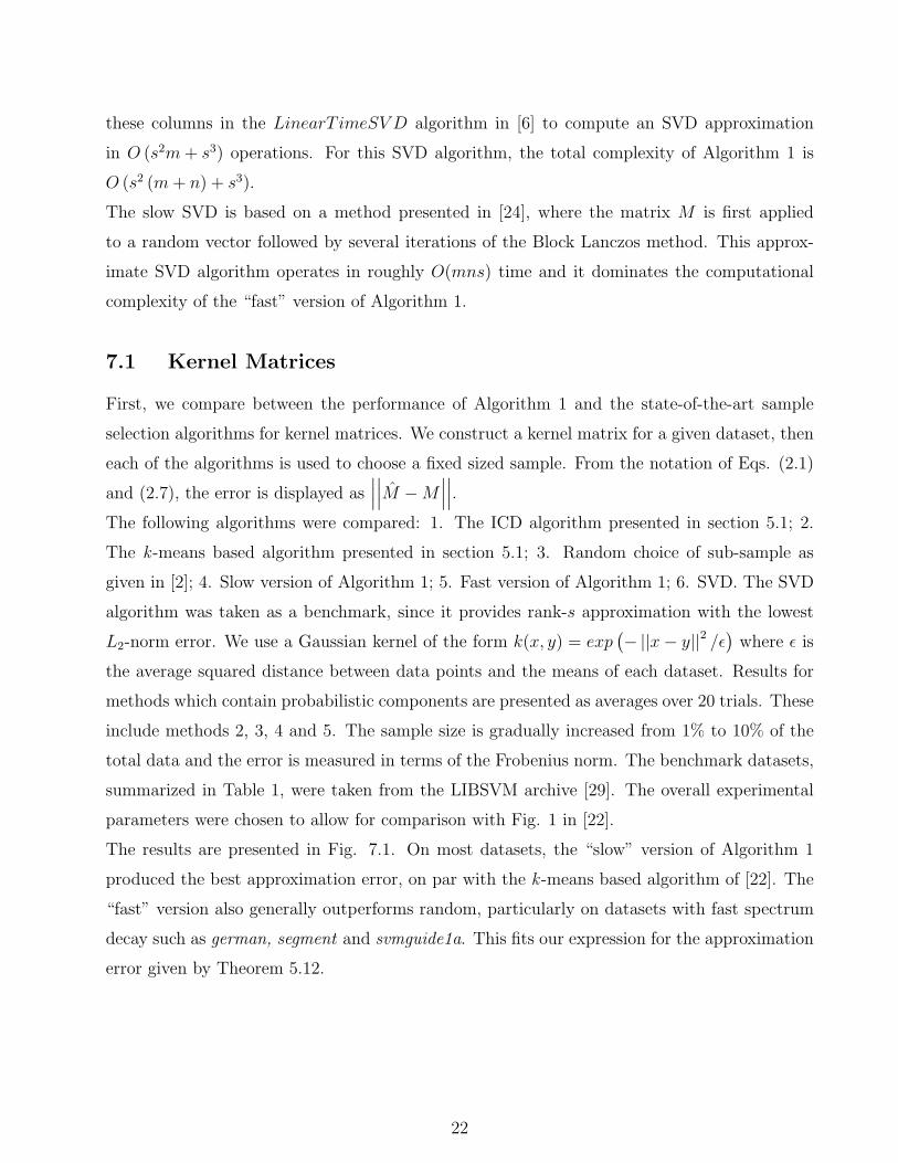
The results are presented in Fig. 7.2. When the spectrum decays slowly, Algorithm 1 has no

advantage over random sample selection. However, the “slow” version has significant advantages

in the presence of large eigen-gaps. This is seen in the “fast decay” and “steps“ graphs.

0.02 0.04 0.06 0.08 0.10

1

2

3

4

5

6

7

x 104

ratio(sample/size)

appr

oxim

atio

n er

ror

(spe

ctra

l nor

m)

slow spectrum decay

randomslow Algorithm 1fast Algorithm 1SVD

0 0.02 0.04 0.06 0.08 0.19.9

9.92

9.94

9.96

9.98

10

10.02

ratio(sample/size)

sing

ular

val

ue

slow decay − matrix spectrum

0.02 0.04 0.06 0.08 0.10

500

1000

1500

2000

2500

ratio(sample/size)

appr

oxim

atio

n er

ror

(spe

ctra

l nor

m)

fast spectrum decay

randomslow Algorithm 1fast Algorithm 1SVD

0 0.02 0.04 0.06 0.08 0.10

5

10

15

20

25

ratio(sample/size)

sing

ular

val

ue

fast decay − matrix spectrum

0.02 0.04 0.06 0.08 0.10

2

4

6

8

x 104

ratio(sample/size)

appr

oxim

atio

n er

ror

(spe

ctra

l nor

m)

steps − fast decay

randomslow Algorithm 1fast Algorithm 1SVD

0 0.02 0.04 0.06 0.08 0.10

200

400

600

800

1000

ratio(sample/size)si

ngul

ar v

alue

fast decay, steps − matrix spectrum

Figure 7.2: Nystrom approximation errors for random matrices. The X-axis is the sampling

ratio, given as sample size divided by matrix size. The Y-axis is the approximation error, given

in L2 norm.

7.3 Non-Singularity of Sample Matrix

We empirically examine the relationship between the Nystrom approximation error and the

non-singularity of the sub-sample matrix. The approximation error is measured in L2-norm

and the non-singularity of AM ∈ Rs×s is measured by the magnitude of σs (AM). We employ

the same three testing matrices as in section 7.2. These feature a non-random spectrum and

random singular subspaces. The sample was chosen to be 5% of the data of the matrix. In

this test, we compare between the random sample selection algorithm and our two versions of

Algorithm 1. Each algorithm was run 100 times on each matrix. The results of each run were

recorded. Figure 7.3 features a log-log scale plot of the approximation error as a function of

σs (AM). When the performance of the different algorithm versions is compared, we arrive at

conclusions similar to those in section 7.2. Our algorithms do no better than random sampling

when the spectrum decay is slow, but consistently outperform random selection in the presence

24

of fast spectrum decay. The performance of the “slow” version of Algorithm 1 is more consistent,

with less variation in accuracy. Figure 7.3 also shows a strong negative correlation between

the variables in all examined matrices. Hence, a large σs (AM) implies small approximation

error. The linear shape of the graphs, drawn in a log-log scale, suggests that this relationship

is exponential. The results hint at a possible extension of the Nystrom procedure to a Monte-

Carlo method: the “fast” version of Algorithm 1 can be run many times, choosing the sample

for which σs (AM) is maximal.

10−4

10−3

10−2

10−1

100

102

103

104

105

106

non−singularity of sample matrix (log scale)

appr

oxim

atio

n er

ror

in 2−

norm

(lo

g sc

ale)

slow spectrum decay

randomslow Algorithm1fast Algorithm1

0 0.02 0.04 0.06 0.08 0.19.9

9.92

9.94

9.96

9.98

10

10.02

ratio (sample/data size)

sing

ular

val

ue

slow decay − matrix spectrum

10−5

10−4

10−3

10−2

10−1

100

101

102

103

104

105

non−singularity of sample matrix (log scale)

appr

oxim

atio

n er

ror

in 2−

norm

(lo

g sc

ale)

fast spectrum decay

randomslow Algorithm1fast Algorithm1

0 0.02 0.04 0.06 0.08 0.10

5

10

15

20

25

ratio (sample/data size)

sing

ular

val

ue

fast decay − matrix spectrum

10−3

10−2

10−1

100

101

102

103

104

105

106

107

non−singularity of sample matrix (log scale)

appr

oxim

atio

n er

ror

in 2−

norm

(lo

g sc

ale)

steps − fast decay

randomslow Algorithm1fast Algorithm1

0 0.02 0.04 0.06 0.08 0.10

200

400

600

800

1000

1200

ratio (sample/data size)

sing

ular

val

ue

fast decay, steps − matrix spectrum

Figure 7.3: Error in Nystrom approximation as a function of σs (AM)

8 Conclusion and Future Research

In this paper, we showed how the Nystrom approximation method can be used to find the

canonical SVD and EVD of a general matrix. In addition, we developed a sample selection

algorithm that operates on general matrices. Experiments performed on real-world kernels

random matrices have shown that the algorithm performs well when the matrix spectrum

exhibits fast decay. Another experiment showed that the non-singularity of the sample matrix

(as measured by the magnitude of the smallest singular value) is exponentially inversely related

25

to the error in approximation.

Future research should focus on further formalizing the relationship between the smallest sin-

gular value of the sample matrix and the Nystrom approximation error. Another interesting

possibility is to find a constrained class of matrices, and develop a sample selection algorithm

for the Nystrom method to take advantage of the constraint. This algorithm can potentially

have much better computational complexity.

References

[1] C.T.H. Baker, The Numerical Treatment of Integral Equations. Oxford: Clarendon Press,

1977.

[2] Charless Fowlkes, Serge Belongie, Fan Chung, Jitendra Malik, ”Spectral Grouping Using

the Nystrom Method,” IEEE Transactions on Pattern Analysis and Machine Intelligence,

vol. 26, no. 2, pp. 214-225, February, 2004.

[3] M. Gu, S.C. Eisenstat, An efficient algorithm for computing a strong rank revealing QR

factorization, SIAM J. Sci. Comput., 17 (1996), pp. 848-869.

[4] C. T. Pan. On the existence and computation of rank-revealing LU factorizations. Linear

Algebra Appl, 316:199-222, 2000.

[5] Golub, G. H. and Van Loan, C. F. 1996 Matrix Computations (3rd Ed.). Johns Hopkins

University Press.

[6] Petros Drineas, Ravi Kannan, and Michael W. Mahoney, Fast Monte Carlo Algorithms

for Matrices II: Computing a Low-Rank Approximation to a Matrix SIAM J. Comput. 36,

158 (2006)

[7] G. W. Stewart, Four algorithms for the efficient computation of truncated QR approxima-

tions to a sparse matrix, Numer. Math., 83 (1999), pp. 313-323.

[8] E. Liberty, F. Woolfe, P.-G. Martinsson, V. Rokhlin, and M. Tygert. Randomized algo-

rithms for the low-rank approximation of matrices. Proc. Natl. Acad. Sci. USA, 104(51):

20167-20172, 2007.

26

[9] A. Deshpande and S. Vempala, Adaptive sampling and fast low-rank matrix approxima-

tion, Technical report TR06-042, Electronic Colloquium on Computational Complexity,

2006.

[10] S. Har-Peled. Low rank matrix approximation in linear time. Manuscript. January 2006.

[11] T. Sarlos, Improved approximation algorithms for large matrices via random projections,

in Proceedings of the 47th Annual IEEE Symposium on Foundations of Computer Science,

2006, pp. 143-152.

[12] S. Fine and K. Scheinberg. Efficient SVM training using low-rank kernel representations.

J. Mach. Learn. Res., 2:243-264, 2001.

[13] P. Drineas and M. W. Mahoney, On the Nystrom method for approximating a Gram matrix

for improved kernel-based learning, J. Machine Learning, 6 (2005), pp. 2153-2175.

[14] P. A. Businger and G. H. Golub, Linear least squares solution by Householder transfor-

mation, Numerische Mathematik, 7 (1965), pp. 269-276.

[15] A. Bjorck and S. Hammarling, A Schur method for the square root of a matrix, Linear

Algebra and Appl., 52/53 (1983) pp. 127-140.

[16] C. K. I. Williams and M. Seeger, Using the Nystrom method to speed up kernel machines,

Advances in Neural Information Processing Systems 2000, MIT Press, 2001.

[17] C. Fowlkes, S. Belongie, and J. Malik, Efficient Spatiotemporal Grouping Using the

Nystrom Method, Proc. IEEE Conf. Computer Vision and Pattern Recognition, Dec. 2001.

[18] S. Belongie, C. Fowlkes, F. Chung, and J. Malik, Spectral Partitioning with Indefinite

Kernels Using the Nystrom Extension, Proc. European Conf. Computer Vision, 2002.

[19] R.R. Coifman and S. Lafon. Geometric harmonics: a novel tool for multiscale out-of-sample

extension of empirical functions. Appl. Comp. Harm. Anal., 21(1):31-52, 2006.

[20] Bengio, Y., Delalleau, O., Roux, N., Paiement, J., Vincent, P., and Ouimet, M. (2004).

Learning eigenfunctions links spectral embedding and kernel PCA. Neural Computation,

16, 2197-2219.

[21] M. Ouimet and Y. Bengio. Greedy spectral embedding. In Proceedings of the Tenth In-

ternational Workshop on Artificial Intelligence and Statistics, 2005.

27

[22] Zhang, K., Tsang, I. W., and Kwok, J. T. 2008. Improved Nystrom low-rank approxima-

tion and error analysis. In Proceedings of the 25th international Conference on Machine

Learning (Helsinki, Finland, July 05 - 09, 2008). ICML ’08, vol. 307. ACM, New York,

NY, 1232-1239.

[23] Sparce greedy matrix approximation for machine learning. A. Smola and B. Scholkopf.

Proceedings of the 17th international conference on machine learning, pp 911-918. June,

2000.

[24] V. Rokhlin, A. Szlam, and M. Tygert, A randomized algorithm for principal component

analysis, Tech. Rep. 0809.2274, arXiv, 2008. Available at http://arxiv.org.

[25] S.T. Roweis and L.K. Saul. Nonlinear dimensionality reduction by Locally Linear Embed-

ding. Science, 290(5500):2323-2326, 2000.

[26] T. Cox and M. Cox. Multidimensional scaling. Chapman & Hall, London, UK, 1994.

[27] H. Hotelling. Analysis of a complex of statistical variables into principal components.

Journal of Educational Psychology, 24:417-441, 1933.

[28] S. Lafon and A.B. Lee. Diffusion maps and coarse-graining: A unified framework for dimen-

sionality reduction, graph partitioning, and data set parameterization. IEEE Transactions

on Pattern Analysis and Machine Intelligence, 28(9):1393-1403, 2006.

[29] Chih-Chung Chang and Chih-Jen Lin, LIBSVM : a library for support vector machines,

2001. Software available at http://www.csie.ntu.edu.tw/∼cjlin/libsvmtools/datasets/

28