Matrix concentration inequalities

STAT 37797: Mathematics of Data Science

Matrix concentration inequalities

Cong Ma

University of Chicago, Autumn 2021

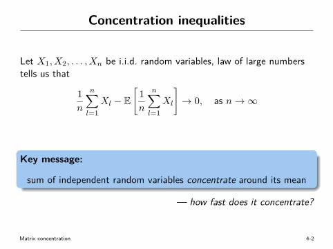
Concentration inequalities

Let X1, X2, . . . , Xn be i.i.d. random variables, law of large numberstells us that

1n

n∑l=1

Xl − E[

1n

n∑l=1

Xl

]→ 0, as n→∞

Key message:

sum of independent random variables concentrate around its mean

— how fast does it concentrate?

Matrix concentration 4-2

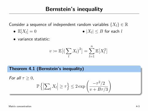
Bernstein’s inequality

Consider a sequence of independent random variables Xl ∈ R• E[Xl] = 0 • |Xl| ≤ B for each l

• variance statistic:

v := E[(∑

l

Xl

)2] =n∑l=1E[X2l

]

Theorem 4.1 (Bernstein’s inequality)

For all τ ≥ 0,

P∣∣∣∑

lXl

∣∣∣ ≥ τ ≤ 2 exp(−τ2/2

v +Bτ/3

)


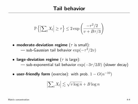
Tail behavior

P∣∣∣∑

lXl

∣∣∣ ≥ τ ≤ 2 exp(−τ2/2

v +Bτ/3

)

• moderate-deviation regime (τ is small):— sub-Gaussian tail behavior exp(−τ2/2v)

• large-deviation regime (τ is large):— sub-exponential tail behavior exp(−3τ/2B) (slower decay)

• user-friendly form (exercise): with prob. 1−O(n−10)∣∣∣∑lXl

∣∣∣ . √v logn+B logn


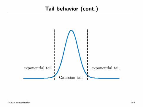
Tail behavior (cont.)

Gaussian tail exponential tail

1


1


1


There are exponential concentration inequalities forspectral norm of sum of independent random matrices

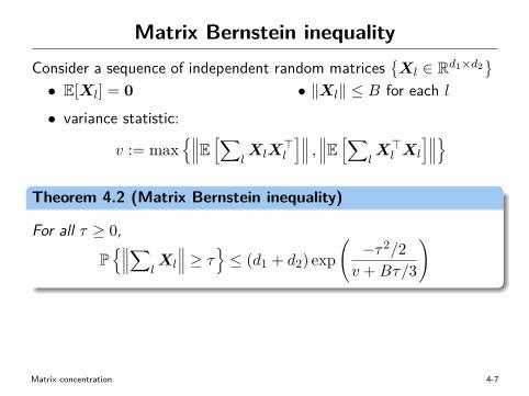
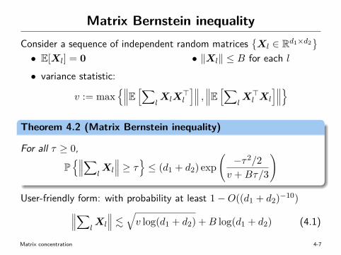
Matrix Bernstein inequalityConsider a sequence of independent random matrices

Xl ∈ Rd1×d2

• E[Xl] = 0 • ‖Xl‖ ≤ B for each l


v := max∥∥∥E [∑

lXlX

>l

]∥∥∥ , ∥∥∥E [∑lX>l Xl

]∥∥∥Theorem 4.2 (Matrix Bernstein inequality)

For all τ ≥ 0,

P∥∥∥∑

lXl

∥∥∥ ≥ τ ≤ (d1 + d2) exp(−τ2/2

v +Bτ/3

)

User-friendly form: with probability at least 1−O((d1 + d2)−10)∥∥∥∑lXl

∥∥∥ . √v log(d1 + d2) +B log(d1 + d2) (4.1)


Matrix Bernstein inequalityConsider a sequence of independent random matrices

Xl ∈ Rd1×d2

• E[Xl] = 0 • ‖Xl‖ ≤ B for each l


v := max∥∥∥E [∑

lXlX

>l

]∥∥∥ , ∥∥∥E [∑lX>l Xl

]∥∥∥Theorem 4.2 (Matrix Bernstein inequality)

For all τ ≥ 0,

P∥∥∥∑

lXl

∥∥∥ ≥ τ ≤ (d1 + d2) exp(−τ2/2

v +Bτ/3

)

User-friendly form: with probability at least 1−O((d1 + d2)−10)∥∥∥∑lXl

∥∥∥ . √v log(d1 + d2) +B log(d1 + d2) (4.1)


This lecture: detailed introduction to matrix Bernstein

An introduction to matrix concentration inequalities— Joel Tropp ’15

Outline

• Background on matrix functions

• Matrix Laplace transform method

• Matrix Bernstein inequality


Background on matrix functions

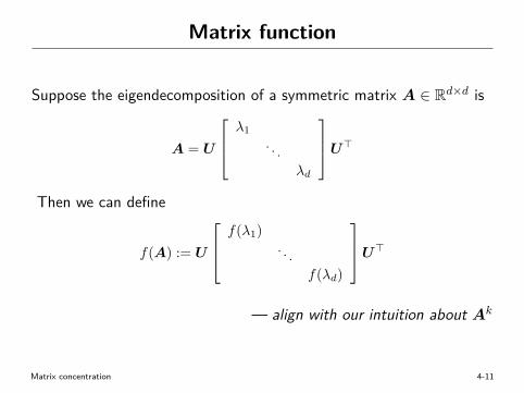
Matrix function

Suppose the eigendecomposition of a symmetric matrix A ∈ Rd×d is

A = U

λ1. . .

λd

U>

Then we can define

f(A) := U

f(λ1). . .

f(λd)

U>

— align with our intuition about Ak


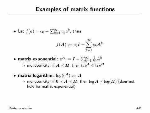
Examples of matrix functions

• Let f(a) = c0 +∑∞k=1 cka

k, then

f(A) := c0I +∞∑k=1

ckAk

• matrix exponential: eA := I +∑∞k=1

1k!A

k

monotonicity: if A H, then tr eA ≤ tr eH

• matrix logarithm: log(eA) := A

monotonicity: if 0 A H, then logA log(H) (does nothold for matrix exponential)


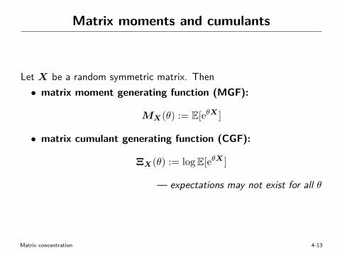
Matrix moments and cumulants

Let X be a random symmetric matrix. Then• matrix moment generating function (MGF):

MX(θ) := E[eθX ]

• matrix cumulant generating function (CGF):

ΞX(θ) := logE[eθX ]

— expectations may not exist for all θ


Matrix Laplace transform method

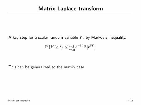
Matrix Laplace transform

A key step for a scalar random variable Y : by Markov’s inequality,

P Y ≥ t ≤ infθ>0

e−θt E[eθY

]

This can be generalized to the matrix case


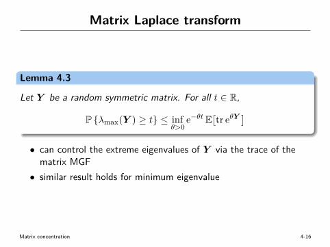
Matrix Laplace transform

Lemma 4.3

Let Y be a random symmetric matrix. For all t ∈ R,

P λmax(Y ) ≥ t ≤ infθ>0

e−θt E[tr eθY

]• can control the extreme eigenvalues of Y via the trace of the

matrix MGF• similar result holds for minimum eigenvalue


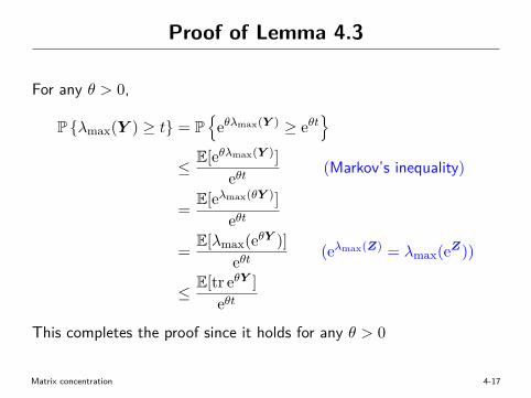
Proof of Lemma 4.3

For any θ > 0,

P λmax(Y ) ≥ t = P

eθλmax(Y ) ≥ eθt

≤ E[eθλmax(Y )]eθt (Markov’s inequality)

= E[eλmax(θY )]eθt

= E[λmax(eθY )]eθt (eλmax(Z) = λmax(eZ))

≤ E[tr eθY ]eθt

This completes the proof since it holds for any θ > 0


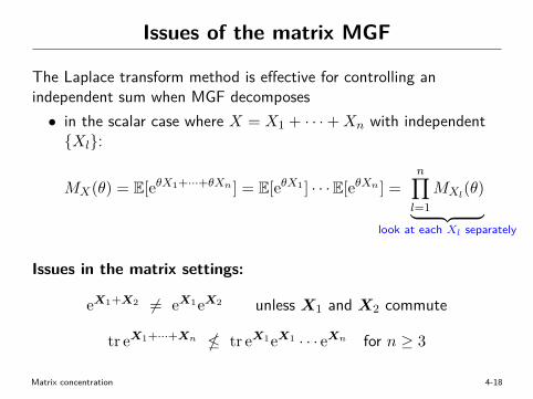
Issues of the matrix MGF

The Laplace transform method is effective for controlling anindependent sum when MGF decomposes• in the scalar case where X = X1 + · · ·+Xn with independentXl:

MX(θ) = E[eθX1+···+θXn ] = E[eθX1 ] · · ·E[eθXn ] =n∏l=1

MXl(θ)︸︷︷︸

look at each Xl separately

Issues in the matrix settings:

eX1+X2 6= eX1eX2 unless X1 and X2 commute

tr eX1+···+Xn tr eX1eX1 · · · eXn for n ≥ 3


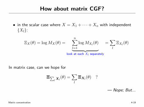
How about matrix CGF?

• in the scalar case where X = X1 + · · ·+Xn with independentXl:

ΞX(θ) = logMX(θ) =n∑l=1

logMXl(θ)︸︷︷︸

look at each Xl separately

=∑l

ΞXl(θ)

In matrix case, can we hope for

Ξ∑lXl

(θ) =∑l

ΞXl(θ) ?

— Nope; But...


Subadditivity of matrix CGF

Fortunately, the matrix CGF satisfies certain subadditivity rules,allowing us to decompose independent matrix components

Lemma 4.4

Consider a finite sequence Xl1≤l≤n of independent randomsymmetric matrices. Then for any θ ∈ R,

E[tr eθ

∑lXl

]︸︷︷︸tr exp

(ΞΣlXl

(θ)) ≤ tr exp

(∑llogE

[eθXl

])︸︷︷︸

tr exp(∑

lΞXl

(θ))

• this is a deep result — based on Lieb’s Theorem!


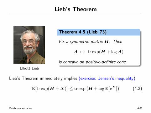
Lieb’s Theorem

Elliott Lieb

Theorem 4.5 (Lieb ’73)

Fix a symmetric matrix H. Then

A 7→ tr exp(H + logA)

is concave on positive-definite cone

Lieb’s Theorem immediately implies (exercise: Jensen’s inequality)

E[tr exp(H + X)

]≤ tr exp

(H + logE

[eX])

(4.2)


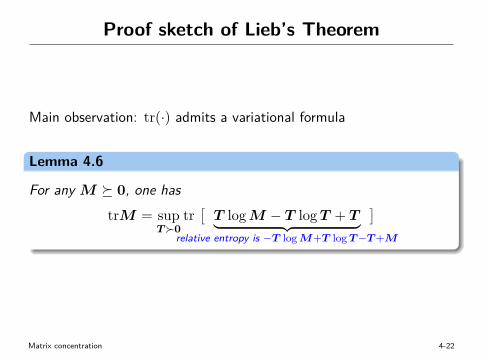
Proof sketch of Lieb’s Theorem

Main observation: tr(·) admits a variational formula

Lemma 4.6

For any M 0, one has

trM = supT0

tr[T logM − T logT + T︸︷︷︸

relative entropy is −T logM+T logT−T+M

]


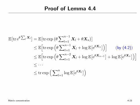
Proof of Lemma 4.4

E[tr eθ

∑lXl]

= E[tr exp

(θ∑n−1

l=1Xl + θXn

)]≤ E

[tr exp

(θ∑n−1

l=1Xl + logE

[eθXn

])](by (4.2))

≤ E[tr exp

(θ∑n−2

l=1Xl + logE

[eθXn−1

]+ logE

[eθXn

])]≤ · · ·

≤ tr exp(∑n

l=1logE

[eθXl

])


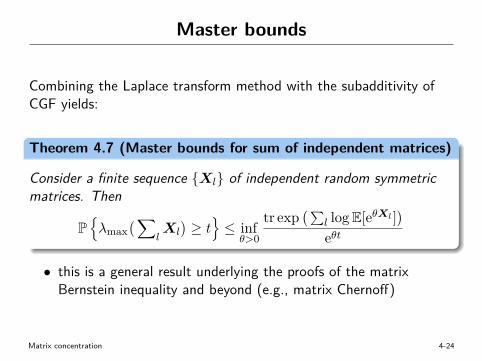
Master bounds

Combining the Laplace transform method with the subadditivity ofCGF yields:

Theorem 4.7 (Master bounds for sum of independent matrices)

Consider a finite sequence Xl of independent random symmetricmatrices. Then

Pλmax

(∑lXl

)≥ t≤ inf

θ>0

tr exp(∑

l logE[eθXl ])

eθt

• this is a general result underlying the proofs of the matrixBernstein inequality and beyond (e.g., matrix Chernoff)


Matrix Bernstein inequality

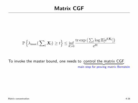
Matrix CGF

Pλmax

(∑lXl

)≥ t≤ inf

θ>0

tr exp(∑

l logE[eθXl ])

eθt

To invoke the master bound, one needs to control the matrix CGF︸︷︷︸main step for proving matrix Bernstein


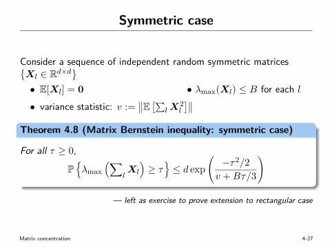
Symmetric case

Consider a sequence of independent random symmetric matricesXl ∈ Rd×d

• E[Xl] = 0 • λmax(Xl) ≤ B for each l

• variance statistic: v :=∥∥E [∑lX

2l

]∥∥Theorem 4.8 (Matrix Bernstein inequality: symmetric case)

For all τ ≥ 0,

Pλmax

(∑lXl

)≥ τ

≤ d exp

(−τ2/2

v +Bτ/3

)

— left as exercise to prove extension to rectangular case


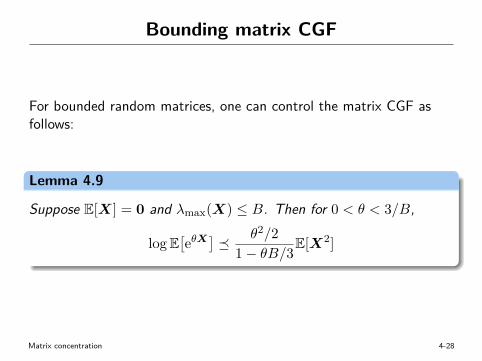
Bounding matrix CGF

For bounded random matrices, one can control the matrix CGF asfollows:

Lemma 4.9

Suppose E[X] = 0 and λmax(X) ≤ B. Then for 0 < θ < 3/B,

logE[eθX

] θ2/2

1− θB/3E[X2]


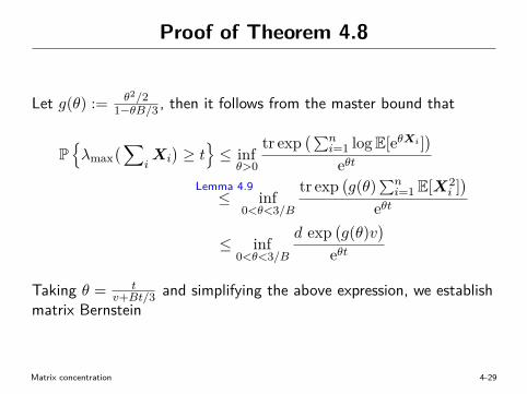
Proof of Theorem 4.8

Let g(θ) := θ2/21−θB/3 , then it follows from the master bound that

Pλmax

(∑iXi)≥ t≤ inf

θ>0

tr exp(∑n

i=1 logE[eθXi ])

eθtLemma 4.9≤ inf

0<θ<3/B

tr exp(g(θ)

∑ni=1 E[X2

i ])

eθt

≤ inf0<θ<3/B

d exp(g(θ)v

)eθt

Taking θ = tv+Bt/3 and simplifying the above expression, we establish

matrix Bernstein


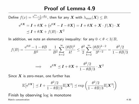
Proof of Lemma 4.9Define f(x) = eθx−1−θx

x2 , then for any X with λmax(X) ≤ B:

eθX = I + θX +(eθX − I − θX

)= I + θX + X · f(X) ·X

I + θX + f(B) ·X2

In addition, we note an elementary inequality: for any 0 < θ < 3/B,

f(B) = eθB − 1− θBB2 = 1

B2

∞∑k=2

(θB)k

k! ≤ θ2

2

∞∑k=2

(θB)k−2

3k−2 = θ2/21− θB/3

=⇒ eθX I + θX + θ2/21− θB/3 ·X

2

Since X is zero-mean, one further has

E[eθX

] I + θ2/2

1− θB/3E[X2] exp(

θ2/21− θB/3E[X2]

)Finish by observing log is monotoneMatrix concentration 4-30

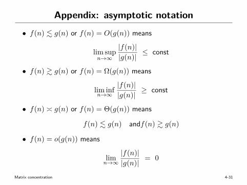
Appendix: asymptotic notation

• f(n) . g(n) or f(n) = O(g(n)) means

lim supn→∞

|f(n)||g(n)| ≤ const

• f(n) & g(n) or f(n) = Ω(g(n)) means

lim infn→∞

|f(n)||g(n)| ≥ const

• f(n) g(n) or f(n) = Θ(g(n)) means

f(n) . g(n) andf(n) & g(n)

• f(n) = o(g(n)) means

limn→∞

|f(n)||g(n)| = 0


Documents

Matrix concentration inequalities