Planning for the future

Matthew Wyble

Econ 495 Project 3

April 17th, 2008

Professor Frank Stafford

Matt Wyble

[1]

Introduction

“He who fails to plan, plans to fail.”

For Project 3, I explored and analyzed both the causes and effects of planning for the

future. In order to determine these outcomes, my analysis looked at a variety of variables from

the early 1970’s that serve as rough metrics for the focus individuals put on planning for their

futures. To consider the effects planning has on various aspects of a person’s life, my analysis

controls for many of the additional factors that impact the ending result, such as wage, gender,

and income level. In order to further bolster this analysis, I used data that is causal when

related to planning (gender, race, age, etc.) in order to determine the underlying motivations

these agents had in using their chosen level planning. Factors such as genetic predisposition

due to background effects are good examples of these obviously causal relationships.

When taken together, these analyses provide some insight into individuals’ motivations

for planning and the payoffs they experience from doing so. The intent of this project is to

provide insight into individuals’ rationality, their ability to plan, and the efficacy of their plans

from a long-term perspective when exogenous factors are controlled for. My hypothesis for

this project is that those who focus on planning should lead to objectively better outcomes on

average than those who do not, because they will be more rational in their long term decision

making and utility maximization.

Methods

For this study, I used data from the Panel Study of Income Dynamics (PSID) from a

number of years. As a proxy for the importance placed on planning, I used a set of variables

that asked respondents if they often planned ahead consistently or if they lived life day by day.

Matt Wyble

[2]

This question was asked between 1968-1972 and 1975 (variables V296, V771, V1438, V2149,

V2744, and V4089, respectively.) I used responses given to a question regarding views of the

future that was asked between 1968 to 1972 (variables V308, V783, V1450, V2161, V2755.) This

question asked the heads of the household how thought about the future and planned. Their

answers were reported on a 5 point scale, with 1 signifying that the respondent “Think[s] a lot

about things that might happen” and 5 signifying that the respondent “Usually just take[s]

things as they come.” The values of 2, 3, and 4 represented a middle ground of ascending

spontaneity acceptance. The respondents who did not answer the planning question (signified

by a value of 9) were omitted for the purposes of these analyses after being shown to have no

statistically predictive power and small size (less than 1% of the sample.) The remaining

variables were used to make a single dummy variable which was given a value of 1 for

responses 1, 2, and 3 and a value of 0 for responses 4 and 5 in the case of both the variables

relating to philosophy towards planning and amount of time spent planning (see the section

labeled “Self reported planning as a proxy for actual planning” for a discussion of the

effectiveness and potential issues of this approach.)

I used a composite of the planning response values for all 6 years to determine what

factors affected their planning. Furthermore, I also examined individual annual responses

separately in the context of a number of potential “event variables” to see if agents were likely

to change their planning tactic after a major event such as a birth or death in the family. Finally,

I used the findings from these analyses to determine what effects planning had on an

individual’s future with respect to various timeframes and numerous aspects of the

respondent’s life: marriage, parenthood, retirement, health, income, and quality of life were

Matt Wyble

[3]

some of the many factors considered. The results of these analyses, their interrelationships,

and their relationship to individuals’ focus on planning for the future are all analyzed and

interpreted.

Results and Discussion

This project explored planning’s effect on a number of variables as mentioned above.

The following is an overview of the interpretable results this project discovered in relation to

the efficacy of planning. The results and their interpretations appear in terms of the

interrelationships between answers in various years to questions regarding planning, the

correlation between self-reported focus on planning and actual planning, factors that influence

individuals’ tendency to plan, and finally the effect that various levels of planning have on other

variables—in other words, how planning more or less affected the respondents’ lives.

Planning over time

In order to determine how people’s planning habits and self reported foci change over

time, I examined all five years (1968-1972) of future focus data combined with the six years of

data (1968-1972, 1975) on planning tactics. As mentioned above, both data sets were divided

into dummy variables representing focus on planning and the future.

Unsurprisingly, these variables exhibited strong correlation, both across individual time

periods as well as over time periods both within and across variables. In other words, those

who “take life as it comes” were far more likely to plan less and live day by day than those that

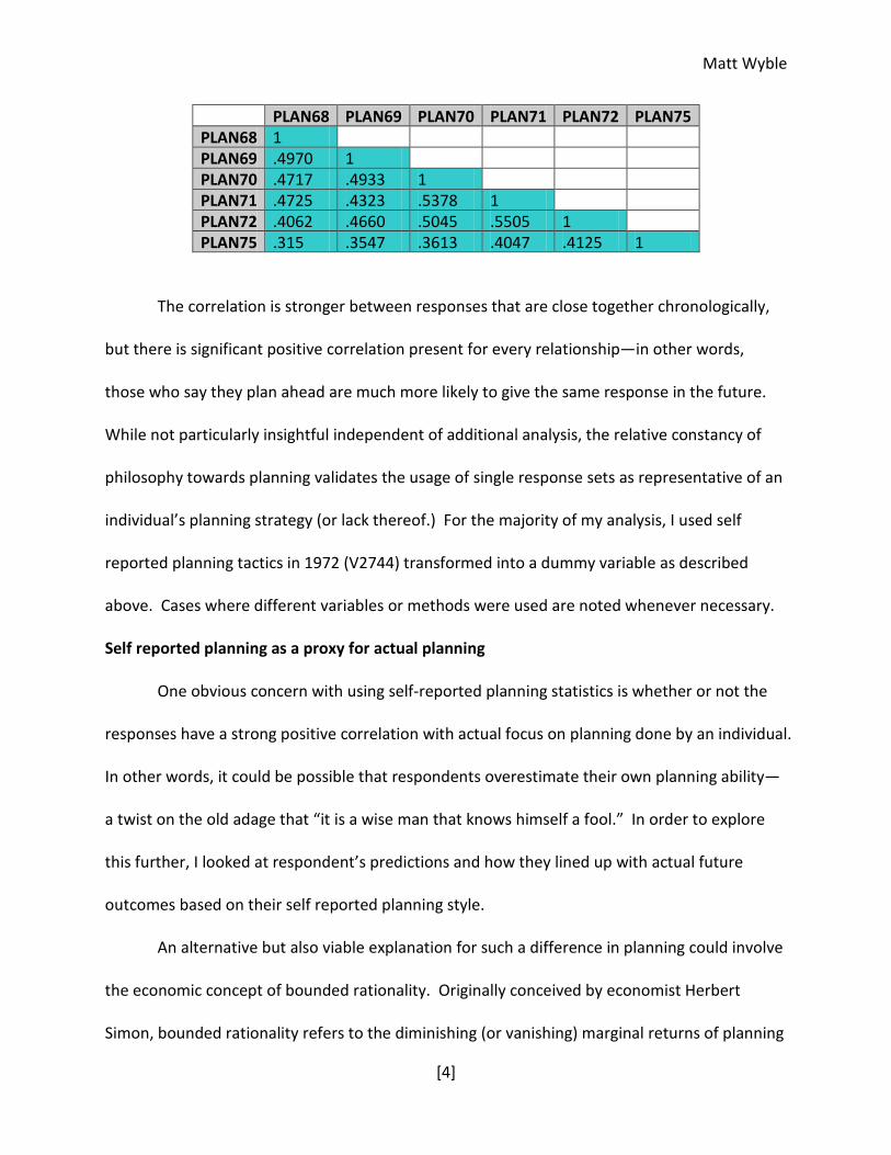
plan for the future and “plan ahead” regularly. The relationships between the planning

variables are indicated in the chart below, where the correlations between years are listed.

Matt Wyble

[4]

PLAN68 PLAN69 PLAN70 PLAN71 PLAN72 PLAN75 PLAN68 1 PLAN69 .4970 1 PLAN70 .4717 .4933 1 PLAN71 .4725 .4323 .5378 1 PLAN72 .4062 .4660 .5045 .5505 1 PLAN75 .315 .3547 .3613 .4047 .4125 1

The correlation is stronger between responses that are close together chronologically,

but there is significant positive correlation present for every relationship—in other words,

those who say they plan ahead are much more likely to give the same response in the future.

While not particularly insightful independent of additional analysis, the relative constancy of

philosophy towards planning validates the usage of single response sets as representative of an

individual’s planning strategy (or lack thereof.) For the majority of my analysis, I used self

reported planning tactics in 1972 (V2744) transformed into a dummy variable as described

above. Cases where different variables or methods were used are noted whenever necessary.

Self reported planning as a proxy for actual planning

One obvious concern with using self-reported planning statistics is whether or not the

responses have a strong positive correlation with actual focus on planning done by an individual.

In other words, it could be possible that respondents overestimate their own planning ability—

a twist on the old adage that “it is a wise man that knows himself a fool.” In order to explore

this further, I looked at respondent’s predictions and how they lined up with actual future

outcomes based on their self reported planning style.

An alternative but also viable explanation for such a difference in planning could involve

the economic concept of bounded rationality. Originally conceived by economist Herbert

Simon, bounded rationality refers to the diminishing (or vanishing) marginal returns of planning

Matt Wyble

[5]

farther into the future due to imperfect forecasting and random events. Unlike simple

macroeconomic models, the act of planning itself requires time and resources that may be

better utilized by other pursuits. Given this, it could be that the “most rational” agents would

be those that plan only to a certain point, instead of sacrificing utility by planning farther into

the future than is efficient.

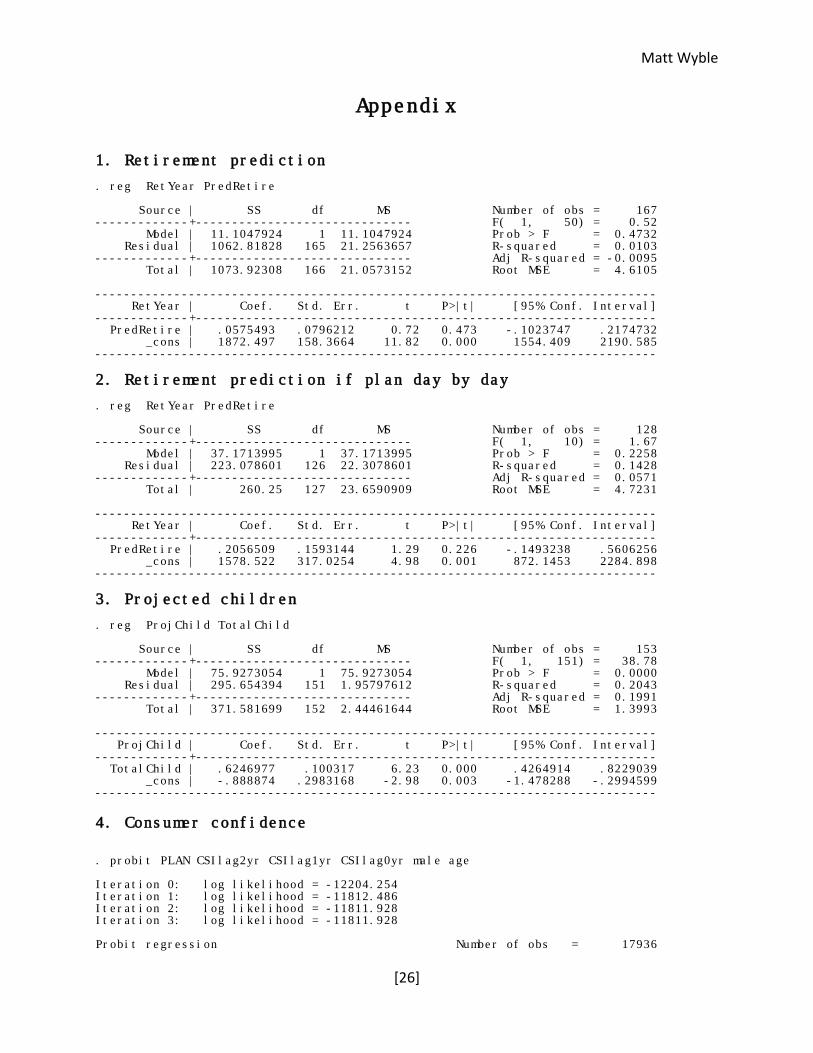
The first variable I considered to determining the validity of self-reported planning was

projected retirement age. I created a new variable for retirement years by combining

responses from a 1978 question about self predicted age of retirement (V5951) with the

respondent’s age in 1972 (V2542), adding six years to account for the time gap between the

questions. Based on this, I created a new variable for the projected year that respondents

thought they would retire, and compared it to actual year of retirement reported in 1995

(ER5071) for both those that were classified as being heavier planners in 1972 and those who

claimed to live more day to day.

I regressed actual retirement year on predicted retirement year for both those that self

reported as planning more1 as well as those that reported planning less.2 As expected, the

standard errors of those who planned more were much smaller—roughly one half the size of

those who reported living for the moment. Another way to consider this is to look at the

average differences between actual and predicted retirement age. On average, those who

planned more were 2.02 years off in their predicted and actual retirement year, while those

who planned less were 2.17 years off. While this is not an extremely large difference, it is

statistically significant at the 5% level. It may be that other factors at play cause it to be an

1 Appendix: Retirement prediction for plan ahead 2 Appendix: Retirement prediction if plan day by day

Matt Wyble

[6]

underestimate of the actual difference—namely, that those who planned more may have been

more responsive to random changes in macroeconomic or individual conditions, and may

therefore be willing to adapt at times when those who planned less would not. Regardless,

those that planned were more accurate when estimating when they would retire than were

those that planned less, as my hypothesis predicted.

Another test that serves as a strong validation of the efficacy of planning and its

correlation with self-reported planning is the link between the predicted number of children

given by a head of household and the actual number of children the household has in the

future. In order to examine this, I compared the projected number of children in 1972 to the

actual total number of children as of 1984. Even when age and other factors had been taken

into account, regressions on the responses of those who planned more had significantly greater

predictive power and lower standard error than of those who were not as future focused.3 Not

surprisingly, this was especially true among women, who have a greater control over the

reproductive process. However, even in the gender nonspecific data, as the attached log

shows, the standard error was 0.0724097 for those who planned more, and 0.100317 for those

who planned less, a clear difference in accuracy between the two groups.

These are some of the many tests that show the predictive accuracy of those that plan

more into the future. In each case, those who live day-to-day have significantly higher

deviations from the predicted output than do those who plan. One interesting question from

this is the planning causality involved—are those who report planning ahead simply better at

forecasting their own actions, or do they instead have an above-average discipline in

3 Appendix: Projected children

Matt Wyble

[7]

conforming to their predictions? This point is certainly both interesting and statistically difficult

to determine. However, it is not central to this project’s analysis of the planning variable. The

important point is that all analyzed prediction data validates the use of self reported planning

focus as a strong proxy for actual planning focus.

Causes of planning

In order to look at planning more in-depth, it is helpful to determine some of the

psychological and economic factors that determine how individuals look at the future. There

are three main areas for this portion of the study: macroeconomic and political changes,

background and demographics, and specific events. This project analyzed each in turn, starting

with macroeconomic and political changes.

Macroeconomic and political changes

For this area of the project, I decided to look at how people’s planning attitudes shift in

aggregate with changing times. Do people plan more during a recession, when war is imminent,

in an election year, etcetera? Unfortunately, the limited time series (only 6 years of responses)

makes some of these questions difficult to answer with a reasonable degree of statistical

significance. However, some strong inferences can still be drawn.

In order to determine how individuals’ perception of the economy might affect how

they plan, this project used data from the Consumer Sentiment index (CSI) (run, of course, by

the University of Michigan.) For the purposes of this analysis I looked at data from 1966 to

1972. The unit-less measure of consumer confidence was collected quarterly at the time. I

generated a new variable by averaging the responses of each quarter in order to create an

average of consumer confidence by year. I also generated a new variable on the change in

Matt Wyble

[8]

consumer confidence from the previous year. Finally, I created a variable containing all

responses to questions of planning for the entire five year period.

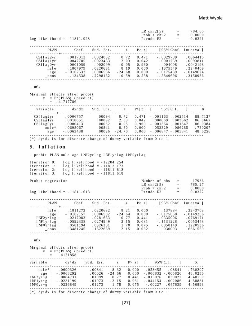
Subsequently, I ran a regression of reported planning style on one year, two year, and

current year CSI values.4 As you can see from the attached regression result, the one year

lagged value of consumer confidence is statistically significant at the 5% level, and is positively

correlated with planning behavior, even when other pertinent factors had been accounted for.

Current consumer confidence has surprisingly little effect on current planning behavior, which

suggests that individual agents take time to modify their behavior in a shifting marketplace and

are reacting to the results of the previous year in their current planning strategy. It appears

that a higher CSI index value in the previous year encourages more planning. In a stronger

market, individuals are able to spend more time forecasting and planning their actions, such as

those dealing with financial investing or saving for college. The reverse often has the opposite

effect—during an economic downturn, individuals have less time and resources to focus on the

future due to their more immediate concerns.

It is interesting that the change from the previous year has a strong negative

relationship to planning percentage. The economic intuition to this is not immediately obvious.

However, there are some reasons why this might occur: one could imagine that individuals

having recently experienced a more challenging economic market may be wary and more

cautious in the following year, even if market conditions have improved dramatically since then.

A similar effect occurs with inflation and planning variables. Using historic data from the

Bureau of Labor Statistics I measured the effect of inflation and lagged inflation on tendency to

4 Appendix: Consumer confidence

Matt Wyble

[9]

plan. When regressed separately against planning tendency, these factors are relatively

significant; however when used in conjunction as in the attached log, they are both statistically

insignificant at the 5% level.5

As can be seen in the attached, inflation is positively correlated with planning. Higher

inflation during the time that the respondents answered the question about planning made it

more likely that they planned more. There are some basic macroeconomic intuitions for this:

inflation tends to be higher in times of high GDP growth, which could also cause people to plan

ahead more. Also, it could be that an influx of money into the stock and bond markets by those

consumers eager to invest in order to prepare for the future lowered the interest rates,

creating lower costs of capital and larger economic investment and growth.

The effect of the previous year’s inflation is also statistically significant when considering

time spent planning in the current year. This is not surprising—consumers in a year after a year

of high inflation would be more likely to focus on the present because they have just

experienced a year where the real value of money dropped rapidly. In such situations, future

returns become less appealing because the real value of money in the future (given sustained

inflation at the same rate) would be lower.

These two examples both underscore the same point: effects from the previous year

shake consumers’ confidence or future outlook and make it more likely that respondents spend

less time planning for the future. When future prospects seem poor, individuals are less likely

to plan for the future. Furthermore, times of poor economic performance create situations

where more immediate needs may trump those of planning for the future—it is certainly more

5 Appendix: Inflation

Matt Wyble

[10]

difficult to plan for the future when one is struggling to make enough money to cover food and

shelter.

Background and demographics

Another area that I hypothesized would be significant were the effects of demographics

and specifics of origin on planning behavior. For this project I focused on gender, race, age,

family background, and other factors in an effort to determine what factors had significant

influence on respondents’ tendency to plan. The first area I considered was gender.

Gender

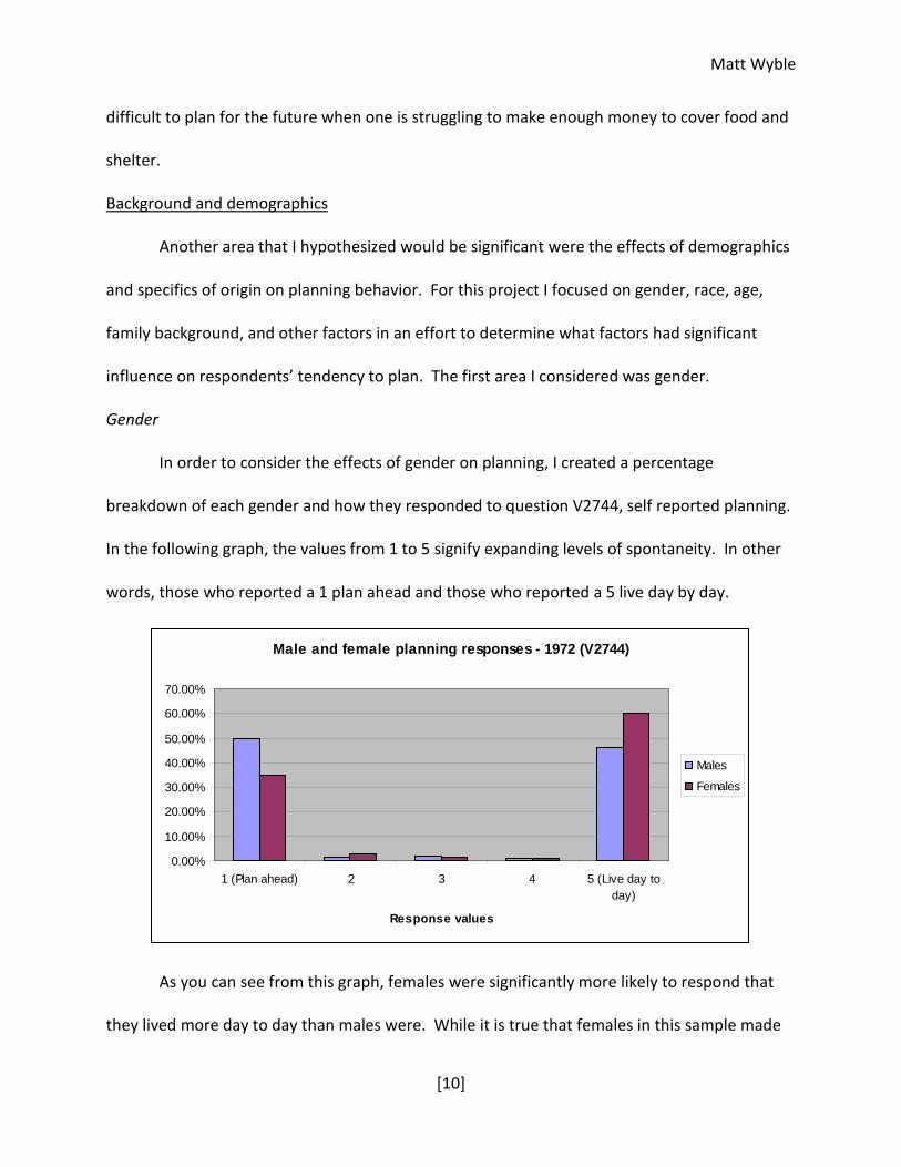
In order to consider the effects of gender on planning, I created a percentage

breakdown of each gender and how they responded to question V2744, self reported planning.

In the following graph, the values from 1 to 5 signify expanding levels of spontaneity. In other

words, those who reported a 1 plan ahead and those who reported a 5 live day by day.

Male and female planning responses - 1972 (V2744)

0.00%

10.00%

20.00%

30.00%

40.00%

50.00%

60.00%

70.00%

1 (Plan ahead) 2 3 4 5 (Live day today)

Response values

Males

Females

As you can see from this graph, females were significantly more likely to respond that

they lived more day to day than males were. While it is true that females in this sample made

Matt Wyble

[11]

less money than the males on average, this relationship holds even when considerations of

income are taken into account. Men are significantly more likely to report planning ahead at

any reasonable level of significance.

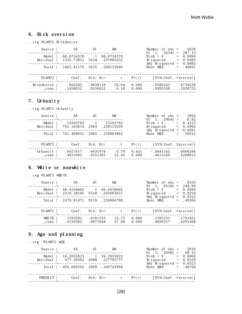
Risk avoidance

One area that can be shown to influence planning behavior significantly is feelings

towards risk. Those who are more risk averse also plan more often. This is in line with

microeconomic concepts of insurance—planning is in a sense a form of personal insurance. The

“payment” is the increased time and energy required to plan ahead, and the payoff is that

future consumption and wealth can be smoothed out as a result. It is not hard to imagine that

more risk averse people would find the marginal utility of spending an additional unit of time or

effort on planning more and would therefore plan ahead more than would someone who is risk

neutral or even risk loving. Unsurprisingly, this relationship holds in the data.6 Using V397, a

metric for risk avoidance based off responses to a number of questions in 1968, it is clear that

being more risk averse is strongly correlated with planning more often.

Childhood home

The area where one spent their childhood was another factor that I hypothesized would

be a significant factor influencing planning strategy. My hypothesis was that those that grew

up in a fast-paced urban environment would plan more than those who were from a rural or

farm environment. In order to test this, I ran regressions on a series of dummy variables

created from V312, a variable that asks the respondents the urbanity of the area where they

grew up. These dummy variables were then regressed against planning. However, no

6 Appendix: Risk aversion

Matt Wyble

[12]

statistically significant variables were found—it appears that those from urban areas are just as

likely as those from rural areas to plan ahead. A similar test using the Beale-Ross Rural-Urban

Continuum Code which ranks urbanity based on a specified metric was also performed.7 This

also produced similarly uncorrelated results—apparently neither the childhood home nor the

current population setting of the respondent affect how they plan for the future.

Race

Race is also a potential factor that could affect how a person plans. This project uses a

set of dummy variables based upon of the original variable (V2828) that corresponds to various

racial identifications. Regressing against these variables creates no statistically significant

relationship. However, regressing on planning with only the dummy variable of white or

nonwhite produced a statistically significant value. This has some intuition behind it—the

dummy variable serves as a measure of the responses of whites and nonwhites in the

population. Those identified as white were far more likely to plan ahead than their nonwhite

counterparts, even when age, region, and income have all been accounted for.8

Age

I took a look at age as a metric and used it in conjunction with V1942 in order to

determine the affects of age on planning. The null hypothesis that age has a positive affect on

planning ahead is rejected at the 1% significance level, and it seems clear that as one gets older,

one does focus more on day-to-day activities.9

7 Appendix: Urbanity 8 Appendix: White or nonwhite 9 Appendix: Age and planning

Matt Wyble

[13]

As you can see, there is a strong, statistically significant negative correlation between

age and time spent planning. In other words, those that are older tend to live more day-by-day

than those that are younger. This holds over the entire sample—running separate regressions

for different age brackets (18-30, 31-40, 41-50, 51-60, 61-70, 71+) yielded similar results across

the board. I found this result interesting, considering the common belief that the young are not

as concerned about the future—this result strongly contradicts the commonly held belief that

youth do not actively consider and plan for their future. There may also be some survivor bias

that diminishes the strength of the relationship—perhaps those who are more methodical in

their planning live longer as a result.

Religion

Another area that had strong significance in determining planning was the respondent’s

religion. As you can see in the graph below, Presbyterians were nearly 15% more likely to plan

than were non-denominational Protestants. This could have something to do with the each

religion’s different theology. For example, some faiths stress trusting in their deity and this may

affect the planning habits of members of different religions or denominations. In addition,

some socioeconomic trends in various denomination membership could also affect these

responses.

Matt Wyble

[14]

There is also reason to think that religion itself might not be a completely causal variable

with respect to planning. For instance, those who plan more may find that the social network

available through some of these organizations advantageous for non-religious reasons. In

addition, a version of Pascal's Wager may be in effect—perhaps those that plan more often

would be attracted to some religions because their planning goes so far as to extend into the

afterlife.10

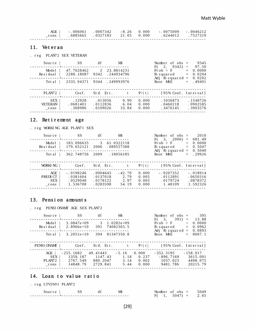
Military veteran status

Since the responses to this question occurred during the Vietnam War and during a time

when military veterans from the Korean War and World War II were middle aged, the

proportion of war veterans in the respondent sample was significant, 31.97% of all respondents.

Using the 1972 responses to whether or not the respondent was a military veteran (V2825), I

regressed their planning tendencies on veteran status and gender (age was shown to be

statistically insignificant.) As you can see in the attached regression, both factors were

10 http://en.wikipedia.org/wiki/Pascal's_Wager

Matt Wyble

[15]

statistically significant at any reasonable significance level. 11 While the gender statistic

remained similar to that of previous regressions, veteran status was also positively correlated.

In other words, those who were veterans were significantly more like to plan ahead, even after

the effects of age, gender, and other variables had been accounted for.

This finding, while not completely surprising, does lead to some interesting results. As

mentioned later, self reported planning tendency has strong positive correlation to individuals’

savings rate—the more you plan, the more you save. With proportionally fewer armed services

veterans today, it seems plausible that the overall drop in average personal savings rates may

have occurred, at least in part, because fewer citizens have been through the sort of traumatic

experiences that war brought over 30 years ago. It makes some intuitive sense that such trying

experiences might make a person more sober and cautious in the future and therefore more

likely to plan ahead, even though notable exceptions such as veterans who have suffered from

Post-Traumatic Stress Disorder have also occurred.

Effects of planning

Having considered the validity and causes of a person’s desire to plan, the final aspect of

study for this project is the effect that planning has on an individual’s current and future life,

actions, and circumstances. In order to provide some clarity, this project is organized into

major thematic sections with subsections for analyses of different portions of the data. The

main areas considered are success and money, family, and health and wellness.

Success and money

11 Appendix: Veteran

Matt Wyble

[16]

When considering how planning affected long-term financial success, I hypothesized

that in most cases, those who planned more would be more successful since they would be less

myopic and more likely to look at the long term effects of their actions instead of merely the

short term gain or loss. While effects that would suggest this sort of success were sometimes

observed, at times additional planning had little (or even negative) influence on future

outcomes. For this portion of the analysis I focused on retirement age, pension level, and

housing debt, and their relationships to self-reported practices of planning ahead.

Retirement

In order to analyze retirement age and how it is affected by planning, I created a set of

dummy variables for the age, sex, and retirement status (retired or still working) of the

respondents in 1980. In order to slightly increase the time distance between questions, I used

responses to a 1971 question about planning (V2161.) For all employment status observations,

I excluded all options except retired and working (i.e. student, housewife, etc.) in order to

control for my desired statistic. The attached results show that even when controlling for age,

one’s self-reported future-looking status is statistically significant in determining the age at

which one will retire.12

There are some interesting results from the regression of retirement age on planning

strategy. Age, planning, and sex are all statistically significant to the 1% level. Retirement and

age have an obvious effect: as age increases, individuals are more likely to be retired. The

effects of sex and focus on planning are even more interesting. Being male significantly

increases the likelihood that one will still be working later in life. This may be because of early

12 Appendix: Retirement age

Matt Wyble

[17]

retirement by mothers. Planning focus has an unexpected effect on retirement: those who

reported being more focused on the future were less likely to be retired. It seems unlikely that

this is the result of poor planning, but rather who those who plan more clearly for the future

were also more likely to work for more years in order to save for a comfortable retirement and

to ensure their financial security. They have a level of risk aversion greater than that of those

who plan less and might retire earlier and with less money and financial security.

Pensions

Pensions are an indispensable portion of retirement income for many Americans.

Therefore, this project hypothesized that individuals who planned more would see significantly

greater pension amounts. To analyze this, the amount of the respondent’s yearly pension

earnings in 1992 (V22045) was regressed on using age, sex, and planning level.13 The null that

planning had no or little effect on pension size was rejected at the 5% significance level, with

those that reported planning ahead having pension payments of $2,163.72 more per year than

those who lived day by day, even when age and gender had been taken into. This certainly ties

into the preceding analysis of working longer if one plans more, but it also has a significantly

positive effect when the extra time spent working is accounted for.

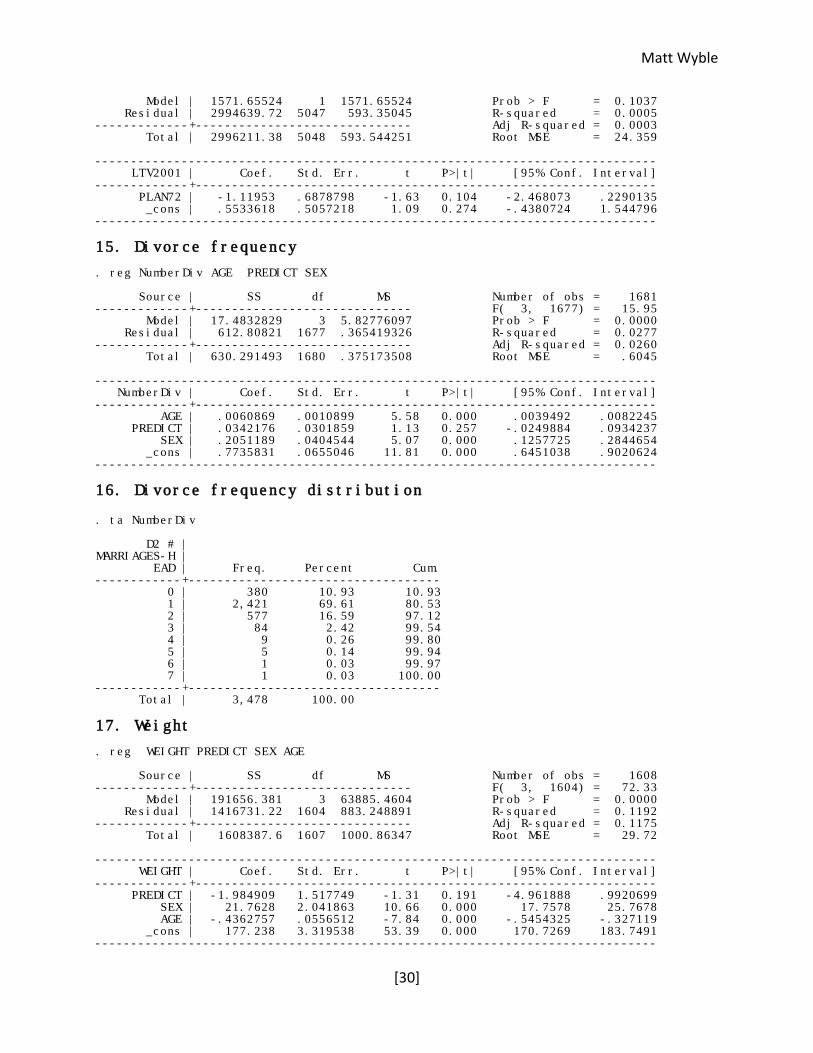
Loan to value ratios

Given the current subprime crisis, the topic of planning and loan-to-value ratios is

especially important. One common characterization of those who are now defaulting on these

types of mortgages is that those who applied for and achieved these mortgages were unable to

pay them off, in part, because they failed to look ahead at the future value of their assets. This

13 Appendix: Pension amounts

Matt Wyble

[18]

assertion is not strongly backed up by tests relating to planning to loan to value ratios. After

considering many different factors, there was not sufficient evidence to reject the null of no

effect, even at the 10% significance level.14

Family

Another large area of interest is how planning more affects familial interaction. While it

does look like some financial success and security comes with planning more, it is not

immediately obvious that similar results will appear in more emotional, qualitative topics that

often permeate considerations of family life. For this area of analysis, I considered topics of

marital success and reproduction rates.

Marital success

Marital success as a function of planning is obviously difficult to determine

quantitatively. How does one define a successful marriage? As an admittedly rough proxy for

this, I used the number of marriages the head of household had had by 1985. The rationale for

this is that those who have been married more often would also have been divorced more

often as well (I assumed that the probability of being widowed was uncorrelated with the

effects of planning.) My hypothesis that those who planned more would have significantly

lower divorce rates was not shown to have statistical significance.15

As you can also see from the attached results, the number of individuals in the sample

that had been married more than 2 times was only 121, which was little more than 3% of the

3999 sample observations.16 However, this relative infrequency could theoretically lead to

14 Appendix: Loan to value ratio 15 Appendix: Divorce frequency 16 Appendix: Divorce frequency distribution

Matt Wyble

[19]

some problems with such regressions, but the outcomes were similar even when all

respondents claiming more than two spouses were removed. In both cases, linear and

quadratic regressions returned values indicating that planning had no statistically significant

effect on divorce rates, even when accounting for other potential variables (age, income,

gender, etc.). It seems that we are less capable of planning matters of the heart than matters

of the pocketbook.

Number of children

To continue in the familial trend, I also looked at the effect of planning methodology on

the number of children that the male head of household had fathered by 1985 (V11844.) These

data points were gathered into the two side-by-side histograms shown below. Families with

more than 12 children were truncated (less than .5% of the sample) to increase the graph

readability.

Number of children born to respondent

39.6

4%

6.80

%

16.3

5%

13.5

3%

9.29

%

4.85

%

2.69

%

2.49

%

1.88

%

0.40

%

0.61

%

0.54

%

0.40

%

25.7

2%

9.47

%

23.9

8%

16.6

6%

10.8

8%

6.04

%

2.62

%

1.41

%

1.21

%

0.60

%

0.54

%

0.34

%

0.20

%

0.00%5.00%

10.00%15.00%20.00%25.00%30.00%35.00%40.00%45.00%

0 1 2 3 4 5 6 7 8 9 10 11 12

Number of children

Live day by day

Plan ahead

These graphs reveal some clear trends: those who plan tend to have more children,

even after age and marital status are controlled for. The most compelling statistic here is

Matt Wyble

[20]

clearly the disparity between those having zero or two children. This is counterbalanced with

the smaller difference in proportions of those having one or three children. Perhaps those who

plan more carefully are able to fulfill at least one part of the American Dream: two kids.

Obviously, there are more than just one or two factors that can be used to more accurately

determine the number of children likely to be born to any head of household, but this chart

represents at least a portion of the difference that is caused by differing planning strategies

among households.

Another consideration is the effect of children on planning—having a child could make

the new parent more forward looking than they had previously been. New concerns such as

saving for college and considering the child’s future become more important than they had

been previously. This statistic almost certainly has causal effects on each other: having a child

affects one’s planning habits, and planning affects the number of children one has.

Health and wellness

The final area of planning’s effects that this analysis explored was the effects of planning

on health and wellness. In order to consider this, I looked at metrics of quality of life, physical

attributes, smoking habits, and overall health.

Quality of life

Rational, utility—maximizing agents in an economy should only plan if it served their

own interests. In other words, additional time and energy spent planning should serve to make

the planner happier in the long run. In order to test this theory, I looked at planners and non-

planners and their self-reported satisfaction over the five year period from 1968 to 1972 using

variable V2788. Following the theme of reporting throughout this project, I eliminated the

Matt Wyble

[21]

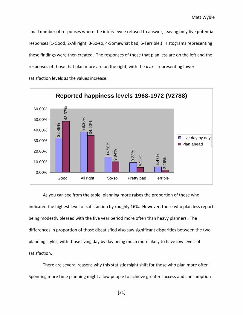
small number of responses where the interviewee refused to answer, leaving only five potential

responses (1-Good, 2-All right, 3-So-so, 4-Somewhat bad, 5-Terrible.) Histograms representing

these findings were then created. The responses of those that plan less are on the left and the

responses of those that plan more are on the right, with the x axis representing lower

satisfaction levels as the values increase.

Reported happiness levels 1968-1972 (V2788)

32.4

5% 38.3

0%

14.5

6%

9.23

%

5.47

%

48.3

7%

34.9

0%

9.94

%

4.53

%

2.26

%

0.00%

10.00%

20.00%

30.00%

40.00%

50.00%

60.00%

Good All right So-so Pretty bad Terrible

Live day by dayPlan ahead

As you can see from the table, planning more raises the proportion of those who

indicated the highest level of satisfaction by roughly 16%. However, those who plan less report

being modestly pleased with the five year period more often than heavy planners. The

differences in proportion of those dissatisfied also saw significant disparities between the two

planning styles, with those living day by day being much more likely to have low levels of

satisfaction.

There are several reasons why this statistic might shift for those who plan more often.

Spending more time planning might allow people to achieve greater success and consumption

Matt Wyble

[22]

levels. However, this comes at the price of additional time spent planning and the potentially

higher stress levels of those who do not adopt a laissez-faire attitude towards the future. Still,

there is a significantly higher proportion of happy people among those who plan more, even

when relevant variables had been accounted for. Furthermore, planning greatly reduces the

probability of having an exceptionally bad five year period, which agrees with the project’s early

analysis of planning as a type of insurance.

Physical health

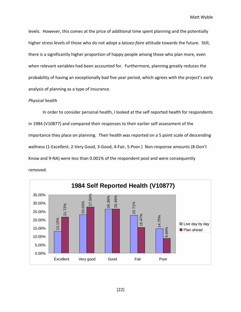
In order to consider personal health, I looked at the self reported health for respondents

in 1984 (V10877) and compared their responses to their earlier self assessment of the

importance they place on planning. Their health was reported on a 5 point scale of descending

wellness (1-Excellent, 2-Very Good, 3-Good, 4-Fair, 5-Poor.) Non-response amounts (8-Don’t

Know and 9-NA) were less than 0.001% of the respondent pool and were consequently

removed.

1984 Self Reported Health (V10877)

13.1

5%

23.0

3% 26.3

6%

22.7

1%

14.7

5%

21.7

2%

27.5

0%

26.4

6%

15.4

7%

8.84

%

0.00%

5.00%

10.00%

15.00%

20.00%

25.00%

30.00%

35.00%

Excellent Very good Good Fair Poor

Live day by dayPlan ahead

Matt Wyble

[23]

The results for this analysis were perhaps the starkest, even when income level, age,

and sex had been accounted for. People who plan more were significantly more likely to report

excellent health. What is most interesting is that the shift came from the “Fair” and “Poor”.

This indicates that planning allows people to avoid the most dire health problems. It is likely

that a combination of behavioral differences and more proliferate and higher quality health

insurance (and higher income) among those who plan contributed significantly to this

avoidance of poor health levels.

Weight

Another area that I considered was the effect of planning on weight in 1980 when

regressed against age, planning ability, and sex. While age and sex were obviously strong

predictors of weight, planning had no statistically significant effect.17 It seems that, as with

their average marriage failure rates, serious planners do not transfer their forward-looking

mindset to their own dietary habits.

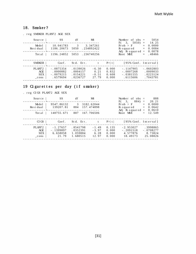
Smoking

The final area that I considered was the effect of planning on smoking cigarettes. To

study this behavior, I looked at two main variables which were collected in 1986: whether or

not the respondent smokes (V13441), and if they do smoke how many cigarettes they smoke a

day (13442.) I regressed each of these individually on planning (1972 value), sex, and age. As

can be seen in the attached regression, whether or not the respondent smokes, planning ahead

is statistically significant and decreases the probability that one smokes by roughly 9%.18

17 Appendix: Weight 18 Appendix: Smoker?

Matt Wyble

[24]

Interestingly, neither gender nor age had a statistically significant impact on whether or not an

individual smoked.

The second area of analysis was the number of cigarettes smoked per day. Running a

regression on these values produced very different results.19 In this case, both age and sex are

statistically significant factors in determining smoking frequency. Furthermore, planning ahead

is not statistically significant, even at the 10% significance level. It seems that although

planning does decrease the likelihood that one will smoke, it does not have a significant effect

on the number of cigarettes smoked if an individual has a habit.

Conclusions

When considering data on planning, basic economic theory would suggest that those

who are forward looking tend to achieve higher levels of utility than those who are more

myopic in their outlook. It is clear that self reported planning attitude is a strong indicator of

actual planning methodology. This correlation can be used to determine the efficacy of

individual’s planning in their own lives as well as being useful in studying those events and

circumstances that cause individuals to plan more.

It is clear that difficult events in individuals’ lives make it more likely that they will plan

in the future—the effects of lagged inflation, consumer confidence, military service, and more

all show this. Additionally, factors such as age, gender, and race have significant effects on how

people plan. However, factors such as current environment (physical, political, and economic)

have varying and often insignificant effects on planning strategy.

19 Appendix: Cigarettes per day (if smoker)

Matt Wyble

[25]

There are many areas wherein those that plan more tend to be rewarded in the

future—better paying jobs, larger pensions, a healthier body, and a higher quality of life are all

likely outcomes of planning more. However, while there are also some areas in which planning

has the sort of positive effect that one would expect, there are also some where no discernible

pattern or relationship could be surmised. This is especially true among the more personal,

emotional, and harder to quantify statistics like marriage, wellness, and personal happiness for

which a numerical value is difficult to determine. However, those who plan are far more likely

to achieve financial security and avoid many of the larger pitfalls encountered by those who

simply live day by day, even as their planning intensity gradually declines with age.

Matt Wyble

[26]

Appendix

1. Retirement prediction . reg RetYear PredRetire Source | SS df MS Number of obs = 167 -------------+------------------------------ F( 1, 50) = 0.52 Model | 11.1047924 1 11.1047924 Prob > F = 0.4732 Residual | 1062.81828 165 21.2563657 R-squared = 0.0103 -------------+------------------------------ Adj R-squared = -0.0095 Total | 1073.92308 166 21.0573152 Root MSE = 4.6105 ------------------------------------------------------------------------------ RetYear | Coef. Std. Err. t P>|t| [95% Conf. Interval] -------------+---------------------------------------------------------------- PredRetire | .0575493 .0796212 0.72 0.473 -.1023747 .2174732 _cons | 1872.497 158.3664 11.82 0.000 1554.409 2190.585 ------------------------------------------------------------------------------

2. Retirement prediction if plan day by day . reg RetYear PredRetire Source | SS df MS Number of obs = 128 -------------+------------------------------ F( 1, 10) = 1.67 Model | 37.1713995 1 37.1713995 Prob > F = 0.2258 Residual | 223.078601 126 22.3078601 R-squared = 0.1428 -------------+------------------------------ Adj R-squared = 0.0571 Total | 260.25 127 23.6590909 Root MSE = 4.7231 ------------------------------------------------------------------------------ RetYear | Coef. Std. Err. t P>|t| [95% Conf. Interval] -------------+---------------------------------------------------------------- PredRetire | .2056509 .1593144 1.29 0.226 -.1493238 .5606256 _cons | 1578.522 317.0254 4.98 0.001 872.1453 2284.898 ------------------------------------------------------------------------------

3. Projected children . reg ProjChild TotalChild Source | SS df MS Number of obs = 153 -------------+------------------------------ F( 1, 151) = 38.78 Model | 75.9273054 1 75.9273054 Prob > F = 0.0000 Residual | 295.654394 151 1.95797612 R-squared = 0.2043 -------------+------------------------------ Adj R-squared = 0.1991 Total | 371.581699 152 2.44461644 Root MSE = 1.3993 ------------------------------------------------------------------------------ ProjChild | Coef. Std. Err. t P>|t| [95% Conf. Interval] -------------+---------------------------------------------------------------- TotalChild | .6246977 .100317 6.23 0.000 .4264914 .8229039 _cons | -.888874 .2983168 -2.98 0.003 -1.478288 -.2994599 ------------------------------------------------------------------------------

4. Consumer confidence . probit PLAN CSIlag2yr CSIlag1yr CSIlag0yr male age Iteration 0: log likelihood = -12204.254 Iteration 1: log likelihood = -11812.486 Iteration 2: log likelihood = -11811.928 Iteration 3: log likelihood = -11811.928 Probit regression Number of obs = 17936

Matt Wyble

[27]

LR chi2(5) = 784.65 Prob > chi2 = 0.0000 Log likelihood = -11811.928 Pseudo R2 = 0.0321 ------------------------------------------------------------------------------ PLAN | Coef. Std. Err. z P>|z| [95% Conf. Interval] -------------+---------------------------------------------------------------- CSIlag2yr | .0017313 .0024032 0.72 0.471 -.0029789 .0064415 CSIlag1yr | .0047785 .0023483 2.03 0.042 .0001759 .0093811 CSIlag0yr | .0001059 .002099 0.05 0.960 -.004008 .0042198 male | .1807979 .0220631 8.19 0.000 .1375549 .2240409 age | -.0162532 .0006586 -24.68 0.000 -.0175439 -.0149624 _cons | -.134538 .2298162 -0.59 0.558 -.5849696 .3158936 ------------------------------------------------------------------------------ . mfx Marginal effects after probit y = Pr(PLAN) (predict) = .41717786 ------------------------------------------------------------------------------ variable | dy/dx Std. Err. z P>|z| [ 95% C.I. ] X ------------+----------------------------------------------------------------- CSIlag2yr | .0006757 .00094 0.72 0.471 -.001163 .002514 88.7137 CSIlag1yr | .0018651 .00092 2.03 0.042 .000069 .003662 86.0667 CSIlag0yr | .0000413 .00082 0.05 0.960 -.001564 .001647 86.0384 male*| .0698067 .00841 8.30 0.000 .053329 .086285 .730207 age | -.0063438 .00026 -24.70 0.000 -.006847 -.005841 48.0256 ------------------------------------------------------------------------------ (*) dy/dx is for discrete change of dummy variable from 0 to 1

5. Inflation . probit PLAN male age INF2yrlag INF1yrlag INF0yrlag Iteration 0: log likelihood = -12204.254 Iteration 1: log likelihood = -11812.173 Iteration 2: log likelihood = -11811.618 Iteration 3: log likelihood = -11811.618 Probit regression Number of obs = 17936 LR chi2(5) = 785.27 Prob > chi2 = 0.0000 Log likelihood = -11811.618 Pseudo R2 = 0.0322 ------------------------------------------------------------------------------ PLAN | Coef. Std. Err. z P>|z| [95% Conf. Interval] -------------+---------------------------------------------------------------- male | .1811272 .0220632 8.21 0.000 .137884 .2243703 age | -.0162157 .0006582 -24.64 0.000 -.0175058 -.0149256 INF2yrlag | .0217083 .0281683 0.77 0.441 -.0335006 .0769171 INF1yrlag | -.0592338 .0274949 -2.15 0.031 -.1131228 -.0053448 INF0yrlag | .0581194 .0326201 1.78 0.075 -.0058149 .1220536 _cons | .3481245 .1622639 2.15 0.032 .030093 .6661559 ------------------------------------------------------------------------------ . mfx Marginal effects after probit y = Pr(PLAN) (predict) = .4171858 ------------------------------------------------------------------------------ variable | dy/dx Std. Err. z P>|z| [ 95% C.I. ] X ---------+-------------------------------------------------------------------- male*| .0699326 .00841 8.32 0.000 .053455 .08641 .730207 age | -.0063292 .00026 -24.66 0.000 -.006832 -.005826 48.0256 INF2yr~g | .0084731 .01099 0.77 0.441 -.013076 .030022 4.40159 INF1yr~g | -.0231199 .01073 -2.15 0.031 -.044154 -.002086 4.58881 INF0yr~g | .0226849 .01273 1.78 0.075 -.00227 .047639 4.56898 ------------------------------------------------------------------------------ (*) dy/dx is for discrete change of dummy variable from 0 to 1

Matt Wyble

[28]

6. Risk aversion . reg PLAN72 RiskAverse Source | SS df MS Number of obs = 5636 -------------+------------------------------ F( 1, 5634) = 287.13 Model | 68.0734378 1 68.0734378 Prob > F = 0.0000 Residual | 1335.73831 5634 .237085252 R-squared = 0.0485 -------------+------------------------------ Adj R-squared = 0.0483 Total | 1403.81175 5635 .249123646 Root MSE = .48691 ------------------------------------------------------------------------------ PLAN72 | Coef. Std. Err. t P>|t| [95% Conf. Interval] -------------+---------------------------------------------------------------- RiskAverse | .066285 .0039118 16.94 0.000 .0586163 .0739536 _cons | .1458032 .0236022 6.18 0.000 .0995338 .1920725 ------------------------------------------------------------------------------

7. Urbanity . reg PLAN72 Urbanity Source | SS df MS Number of obs = 2966 -------------+------------------------------ F( 1, 2964) = 0.62 Model | .15503763 1 .15503763 Prob > F = 0.4312 Residual | 741.343614 2964 .250115929 R-squared = 0.0002 -------------+------------------------------ Adj R-squared = -0.0001 Total | 741.498651 2965 .250083862 Root MSE = .50012 ------------------------------------------------------------------------------ PLAN72 | Coef. Std. Err. t P>|t| [95% Conf. Interval] -------------+---------------------------------------------------------------- Urbanity | .0027617 .0035078 0.79 0.431 -.0041162 .0096396 _cons | .4911992 .0151381 32.45 0.000 .4615169 .5208815 ------------------------------------------------------------------------------

8. White or nonwhite . reg PLAN72 WHITE Source | SS df MS Number of obs = 9520 -------------+------------------------------ F( 1, 9518) = 248.00 Model | 60.4336605 1 60.4336605 Prob > F = 0.0000 Residual | 2319.38105 9518 .243683657 R-squared = 0.0254 -------------+------------------------------ Adj R-squared = 0.0253 Total | 2379.81471 9519 .250006798 Root MSE = .49364 ------------------------------------------------------------------------------ PLAN72 | Coef. Std. Err. t P>|t| [95% Conf. Interval] -------------+---------------------------------------------------------------- WHITE | .1593591 .0101193 15.75 0.000 .1395231 .1791951 _cons | .4150382 .0071944 57.69 0.000 .4009357 .4291408 ------------------------------------------------------------------------------

9. Age and planning . reg PLAN72 AGE Source | SS df MS Number of obs = 2010 -------------+------------------------------ F( 1, 2008) = 68.15 Model | 16.2055823 1 16.2055823 Prob > F = 0.0000 Residual | 477.49392 2008 .237795777 R-squared = 0.0328 -------------+------------------------------ Adj R-squared = 0.0323 Total | 493.699502 2009 .245743904 Root MSE = .48764 ------------------------------------------------------------------------------ PREDICT | Coef. Std. Err. t P>|t| [95% Conf. Interval] -------------+----------------------------------------------------------------

Matt Wyble

[29]

AGE | -.006061 .0007342 -8.26 0.000 -.0075009 -.0046212 _cons | .6885665 .0327183 21.05 0.000 .6244012 .7527319 ------------------------------------------------------------------------------

11. Veteran . reg PLAN72 SEX VETERAN Source | SS df MS Number of obs = 9345 -------------+------------------------------ F( 2, 9342) = 97.50 Model | 47.7628462 2 23.8814231 Prob > F = 0.0000 Residual | 2288.18087 9342 .244934796 R-squared = 0.0204 -------------+------------------------------ Adj R-squared = 0.0202 Total | 2335.94371 9344 .249993976 Root MSE = .49491 ------------------------------------------------------------------------------ PLAN72 | Coef. Std. Err. t P>|t| [95% Conf. Interval] -------------+---------------------------------------------------------------- SEX | .12928 .013056 9.90 0.000 .1036873 .1548726 VETERAN | .0681401 .0112836 6.04 0.000 .0460218 .0902585 _cons | .368986 .0109026 33.84 0.000 .3476145 .3903576 ------------------------------------------------------------------------------

12. Retirement age . reg WORKING AGE PLAN71 SEX Source | SS df MS Number of obs = 2010 -------------+------------------------------ F( 3, 2006) = 681.49 Model | 183.096635 3 61.0322118 Prob > F = 0.0000 Residual | 179.652121 2006 .089557388 R-squared = 0.5047 -------------+------------------------------ Adj R-squared = 0.5040 Total | 362.748756 2009 .18056185 Root MSE = .29926 ------------------------------------------------------------------------------ WORKING | Coef. Std. Err. t P>|t| [95% Conf. Interval] -------------+---------------------------------------------------------------- AGE | -.0198246 .0004643 -42.70 0.000 -.0207352 -.018914 PREDICT | .0381604 .0137018 2.79 0.005 .0112891 .0650316 SEX | .0529048 .0178122 2.97 0.003 .0179724 .0878372 _cons | 1.536708 .0283598 54.19 0.000 1.48109 1.592326 ------------------------------------------------------------------------------

13. Pension amounts . reg PENSIONAMT AGE SEX PLAN72 Source | SS df MS Number of obs = 395 -------------+------------------------------ F( 3, 391) = 13.88 Model | 3.0847e+09 3 1.0282e+09 Prob > F = 0.0000 Residual | 2.8966e+10 391 74082365.5 R-squared = 0.0962 -------------+------------------------------ Adj R-squared = 0.0893 Total | 3.2051e+10 394 81347350.8 Root MSE = 8607.1 ------------------------------------------------------------------------------ PENSIONAMT | Coef. Std. Err. t P>|t| [95% Conf. Interval] -------------+---------------------------------------------------------------- AGE | -255.1682 49.41443 -5.16 0.000 -352.3195 -158.017 SEX | 1359.187 1147.43 1.18 0.237 -896.7169 3615.091 PLAN72 | 2767.549 880.2047 3.14 0.002 1037.023 4498.075 _cons | 14848.79 2729.841 5.44 0.000 9481.786 20215.79 ------------------------------------------------------------------------------

14. Loan to value ratio . reg LTV2001 PLAN72 Source | SS df MS Number of obs = 5049 -------------+------------------------------ F( 1, 5047) = 2.65

Matt Wyble

[30]

Model | 1571.65524 1 1571.65524 Prob > F = 0.1037 Residual | 2994639.72 5047 593.35045 R-squared = 0.0005 -------------+------------------------------ Adj R-squared = 0.0003 Total | 2996211.38 5048 593.544251 Root MSE = 24.359 ------------------------------------------------------------------------------ LTV2001 | Coef. Std. Err. t P>|t| [95% Conf. Interval] -------------+---------------------------------------------------------------- PLAN72 | -1.11953 .6878798 -1.63 0.104 -2.468073 .2290135 _cons | .5533618 .5057218 1.09 0.274 -.4380724 1.544796 ------------------------------------------------------------------------------

15. Divorce frequency . reg NumberDiv AGE PREDICT SEX Source | SS df MS Number of obs = 1681 -------------+------------------------------ F( 3, 1677) = 15.95 Model | 17.4832829 3 5.82776097 Prob > F = 0.0000 Residual | 612.80821 1677 .365419326 R-squared = 0.0277 -------------+------------------------------ Adj R-squared = 0.0260 Total | 630.291493 1680 .375173508 Root MSE = .6045 ------------------------------------------------------------------------------ NumberDiv | Coef. Std. Err. t P>|t| [95% Conf. Interval] -------------+---------------------------------------------------------------- AGE | .0060869 .0010899 5.58 0.000 .0039492 .0082245 PREDICT | .0342176 .0301859 1.13 0.257 -.0249884 .0934237 SEX | .2051189 .0404544 5.07 0.000 .1257725 .2844654 _cons | .7735831 .0655046 11.81 0.000 .6451038 .9020624 ------------------------------------------------------------------------------

16. Divorce frequency distribution . ta NumberDiv D2 # | MARRIAGES-H | EAD | Freq. Percent Cum. ------------+----------------------------------- 0 | 380 10.93 10.93 1 | 2,421 69.61 80.53 2 | 577 16.59 97.12 3 | 84 2.42 99.54 4 | 9 0.26 99.80 5 | 5 0.14 99.94 6 | 1 0.03 99.97 7 | 1 0.03 100.00 ------------+----------------------------------- Total | 3,478 100.00

17. Weight . reg WEIGHT PREDICT SEX AGE Source | SS df MS Number of obs = 1608 -------------+------------------------------ F( 3, 1604) = 72.33 Model | 191656.381 3 63885.4604 Prob > F = 0.0000 Residual | 1416731.22 1604 883.248891 R-squared = 0.1192 -------------+------------------------------ Adj R-squared = 0.1175 Total | 1608387.6 1607 1000.86347 Root MSE = 29.72 ------------------------------------------------------------------------------ WEIGHT | Coef. Std. Err. t P>|t| [95% Conf. Interval] -------------+---------------------------------------------------------------- PREDICT | -1.984909 1.517749 -1.31 0.191 -4.961888 .9920699 SEX | 21.7628 2.041863 10.66 0.000 17.7578 25.7678 AGE | -.4362757 .0556512 -7.84 0.000 -.5454325 -.327119 _cons | 177.238 3.319538 53.39 0.000 170.7269 183.7491 ------------------------------------------------------------------------------

Matt Wyble

[31]

18. Smoker? . reg SMOKER PLAN72 AGE SEX Source | SS df MS Number of obs = 5054 -------------+------------------------------ F( 3, 5050) = 14.25 Model | 10.041783 3 3.347261 Prob > F = 0.0000 Residual | 1186.20673 5050 .234892422 R-squared = 0.0084 -------------+------------------------------ Adj R-squared = 0.0078 Total | 1196.24852 5053 .236740256 Root MSE = .48466 ------------------------------------------------------------------------------ SMOKER | Coef. Std. Err. t P>|t| [95% Conf. Interval] -------------+---------------------------------------------------------------- PLAN72 | -.0875354 .0139026 -6.30 0.000 -.1147905 -.0602803 AGE | .0000882 .0004157 0.21 0.832 -.0007268 .0009033 SEX | -.0079215 .0154221 -0.51 0.608 -.0381555 .0223124 _cons | .6579694 .0236727 27.79 0.000 .6115606 .7043781 ------------------------------------------------------------------------------

19 Cigarettes per day (if smoker) . reg CIGS PLAN72 AGE SEX Source | SS df MS Number of obs = 888 -------------+------------------------------ F( 3, 884) = 20.21 Model | 9547.86132 3 3182.62044 Prob > F = 0.0000 Residual | 139207.81 884 157.474898 R-squared = 0.0642 -------------+------------------------------ Adj R-squared = 0.0610 Total | 148755.671 887 167.706506 Root MSE = 12.549 ------------------------------------------------------------------------------ CIGS | Coef. Std. Err. t P>|t| [95% Conf. Interval] -------------+---------------------------------------------------------------- PLAN72 | -1.27657 .8541798 -1.49 0.135 -2.953027 .3998865 AGE | -.1399897 .0352391 -3.97 0.000 -.2091518 -.0708277 SEX | 6.658058 1.059884 6.28 0.000 4.577876 8.73824 _cons | 21.79 1.680515 12.97 0.000 18.49173 25.08826 ------------------------------------------------------------------------------