98:1883-1897, 2007. First published Jun 27, 2007;  doi:10.1152/jn.00233.2007 J NeurophysiolWood and Mark C. W. van Rossum Matthijs A. A. van der Meer, James J. Knierim, D. Yoganarasimha, Emma R.

You might find this additional information useful...

61 articles, 28 of which you can access free at: This article cites http://jn.physiology.org/cgi/content/full/98/4/1883#BIBL

3 other HighWire hosted articles: This article has been cited by

  [PDF]  [Full Text]  [Abstract]

, January 14, 2009; 29 (2): 493-507. J. Neurosci.B. J. Clark, A. Sarma and J. S. Taube

Interpeduncular NucleusHead Direction Cell Instability in the Anterior Dorsal Thalamus after Lesions of the 

[PDF]  [Full Text]  [Abstract], March 28, 2009; 367 (1891): 1063-1078. Phil Trans R Soc A

R. Nijhawan and S. Wu Compensating time delays with neural predictions: are predictions sensory or motor?

  [PDF]  [Full Text]  [Abstract]

, November 18, 2009; 29 (46): 14521-14533. J. Neurosci.S. Taube G. M. Muir, J. E. Brown, J. P. Carey, T. P. Hirvonen, C. C. Della Santina, L. B. Minor and J.

in the Freely Moving ChinchillaDisruption of the Head Direction Cell Signal after Occlusion of the Semicircular Canals

including high-resolution figures, can be found at: Updated information and services http://jn.physiology.org/cgi/content/full/98/4/1883

can be found at: Journal of Neurophysiologyabout Additional material and information http://www.the-aps.org/publications/jn

This information is current as of September 16, 2010 .  

http://www.the-aps.org/.American Physiological Society. ISSN: 0022-3077, ESSN: 1522-1598. Visit our website at (monthly) by the American Physiological Society, 9650 Rockville Pike, Bethesda MD 20814-3991. Copyright © 2007 by the

publishes original articles on the function of the nervous system. It is published 12 times a yearJournal of Neurophysiology

on Septem

ber 16, 2010 jn.physiology.org

Dow

nloaded from

Anticipation in the Rodent Head Direction System Can Be Explained by anInteraction of Head Movements and Vestibular Firing Properties

Matthijs A. A. van der Meer,1 James J. Knierim,4 D. Yoganarasimha,4 Emma R. Wood,2

and Mark C. W. van Rossum3

1Neuroinformatics Doctoral Training Centre, 2Centre for Cognitive and Neural Systems, and 3Institute for Adaptive and NeuralComputation, University of Edinburgh, Edinburgh, United Kingdom; and 4Department of Neurobiology and Anatomy, W. M. Keck Centerfor the Neurobiology of Learning and Memory, The University of Texas Medical School, Houston, Texas

Submitted 4 March 2007; accepted in final form 25 June 2007

van der Meer MA, Knierim JJ, Yoganarasimha D, Wood ER, vanRossum MC. Anticipation in the rodent head direction system can beexplained by an interaction of head movements and vestibular firingproperties. J Neurophysiol 98: 1883–1897, 2007. First published June27, 2007; doi:10.1152/jn.00233.2007. The rodent head-direction (HD)system, which codes for the animal’s head direction in the horizontalplane, is thought to be critically involved in spatial navigation.Electrophysiological recording studies have shown that HD cells cananticipate the animal’s HD by up to 75–80 ms. The origin of thisanticipation is poorly understood. In this modeling study, we providea novel explanation for HD anticipation that relies on the firingproperties of neurons afferent to the HD system. By incorporatingspike rate adaptation and postinhibitory rebound as observed inmedial vestibular nucleus neurons, our model produces realistic an-ticipation on a large corpus of rat movement data. In addition, HDanticipation varies between recording sessions of the same cell,between active and passive movement, and between different studies.Such differences do not appear to be correlated with behavioral variablesand cannot be accounted for using earlier models. In the present model,anticipation depends on the power spectrum of the head movements. Bydirect comparison with recording data, we show that the model explains60–80% of the observed anticipation variability. We conclude that HDafferent dynamics and the statistics of rat head movements are importantin generating HD anticipation. This result contributes to understandingthe functional circuitry of the HD system and has methodological impli-cations for studies of HD anticipation.

I N T R O D U C T I O N

To support complex behaviors, the brain must convert sen-sory information into abstract and persistent representations.The rodent head-direction (HD) system (Ranck 1984; Sharp etal. 2001a; Taube et al. 1990a,b; Wiener and Taube 2005) is astriking example of a “cognitive” representation without adirect sensory correlate. A given HD cell is maximally activewhen the animal’s head is facing that cell’s preferred firingdirection in the horizontal plane, irrespective of location orongoing behaviors (Taube et al. 1990a). Different cells havedifferent preferred directions, evenly covering the directionalspace to form a “neural compass” representing the animal’scurrent HD (Baird et al. 2001; Johnson et al. 2005). Thecompass can be updated by visual inputs, yet it persists indarkness (Blair and Sharp 1996; Goodridge and Taube 1995;but see Chen et al. 1994; Mizumori and Williams 1993). The

HD system is thought to be a critical component for severalforms of spatial navigation (Gallistel 1990; McNaughton et al.1991, 1996, 2006; Redish 1999; Taube 1998; but see Dud-chenko et al. 2005; Muir and Taube 2002).

When viewed as a sensory system, HD cells would beexpected to encode with some delay or time lag caused bytransduction, transmission, and other delays. However, HD cellactivity (in some brain areas) correlates best with future HD, asrevealed by time-slide analyses (Blair and Sharp 1995; Taubeand Muller 1998). Following the HD literature, we refer to thiseffect as anticipation; however, it should be noted that this doesnot necessarily imply an active prediction process. Experimen-tally, anticipatory time intervals (ATIs) of up to 75–80 mshave been observed (Blair et al. 1997; Stackman and Taube1998; note erratum). These ATIs vary both between differentHD cells and between different recording sessions of the samecell. Blair et al. (1997) report that ATIs of the same HD cellrecorded during multiple recording sessions can differ by asmuch as 50 ms, although on average, within-cell ATI variabil-ity is smaller than that between cells (Blair et al. 1997; Taubeand Muller 1998). Additionally, estimates of the mean ATI(recorded from the same brain area, but across cells andsubjects) can differ by 25–30 ms between different studies(comparing Blair et al. 1998 and Stackman and Taube 1998)including studies from the same group (comparing Bassett etal. 2005 and Taube and Muller 1998). Finally, a recent report(Bassett et al. 2005) showed an ATI increase of 40 ms whenrats were passively rotated compared with freely moving.Where examined, such ATI differences could not be explainedby behavioral variables such as average turning velocity orturning bias (Bassett et al. 2005; Blair et al. 1997). Thusalthough individual cells to some extent have a characteristicATI, there are also unexplained differences.

Previous theoretical models exploring the possible origin of HDanticipation (Goodridge and Touretzky 2000; Redish et al. 1996;Xie et al. 2002) do not account for these variations. Additionally,they fall short of generating the long ATIs observed in the lateralmammillary nuclei (LMN): simulations reported in Goodridgeand Touretzky (2000) only resulted in 30 ms of anticipation in themost favorable case, whereas mean experimental values range upto 67 ms (Stackman and Taube 1998).

In this modeling study, we present a novel hypothesis for thegeneration of anticipation in the HD system. Like authors of

Present address and address for reprint requests and other correspondence:M.A.A. van der Meer, Dept. of Neuroscience, University of Minnesota, 6-145Jackson Hall, 321 Church St. SE, Minneapolis, MN 55455 (E-mail:vande642@umn.edu).

The costs of publication of this article were defrayed in part by the paymentof page charges. The article must therefore be hereby marked “advertisement”in accordance with 18 U.S.C. Section 1734 solely to indicate this fact.

J Neurophysiol 98: 1883–1897, 2007.First published June 27, 2007; doi:10.1152/jn.00233.2007.

18830022-3077/07 $8.00 Copyright © 2007 The American Physiological Societywww.jn.org

on Septem

ber 16, 2010 jn.physiology.org

Dow

nloaded from

previous models (e.g., Redish et al. 1996; Skaggs et al. 1995;Song and Wang 2005), we assume that the HD system inte-grates angular head velocity (AHV) from the vestibular sys-tem. However, we consider the firing dynamics of vestibularneurons such that instead of being updated by a perfect ves-tibular AHV signal, the HD system effectively receives ahigh-pass filtered version of that signal, which results inanticipation. This filtering is achieved by incorporating theeffects of vestibular spike rate adaptation (a decreasing firingrate response to a constant persistent stimulus) and postinhibi-tory rebound firing (a transient increase in firing rate followingrelease from inhibitory input) as reported in Sekirnjak and duLac (2002). We show that for physiological amounts of ves-tibular adaptation and rebound, the model generates realisticATIs on a large set of rat tracking data. Critically, the resultinganticipation depends on the statistics of the input head move-

ment pattern, thus providing an explanation for the observedATI variability as well as way to test the model directly againstexperimental ATI values. In support of our hypothesis, we firstshow that rats exhibit variations in the statistics of their headmovements. ATIs generated by the model on these head move-ments correlate strongly with experimental values, accounting forover half of the experimentally observed ATI variability.

M E T H O D S

Ring attractor network model

Our model of the HD system uses a “ring” attractor network ofnonlinear units with generic rate-based dynamics, similar to previousmodels (Redish et al. 1996; Skaggs et al. 1995; Trappenberg 2002;Zhang 1996). However, the critical component of the model lies in thedynamics of the input signal to this network (described in Inputdynamics). Figure 1A shows a schematic of the complete model, of

updateHDring

in

out

adaptation rebound

leftMVNunittracking

data frommoving rat

inputangular head velocity

modified outputangular head velocity

0 2

120

0 2

0 2

120

0 2

adaptationreboundMVN activity

time (s) time (s)

head

dire

ctio

n (d

eg)

0 2

-30

30

actual HDmodel outputshifted output

time (s)

inp

utA

HV

(º/s

)M

VN

act

ivity

left rightC

A

D

E left right left

gain

γ

A Rτ τ

1 2

3

4 5

B

rightMVNunit

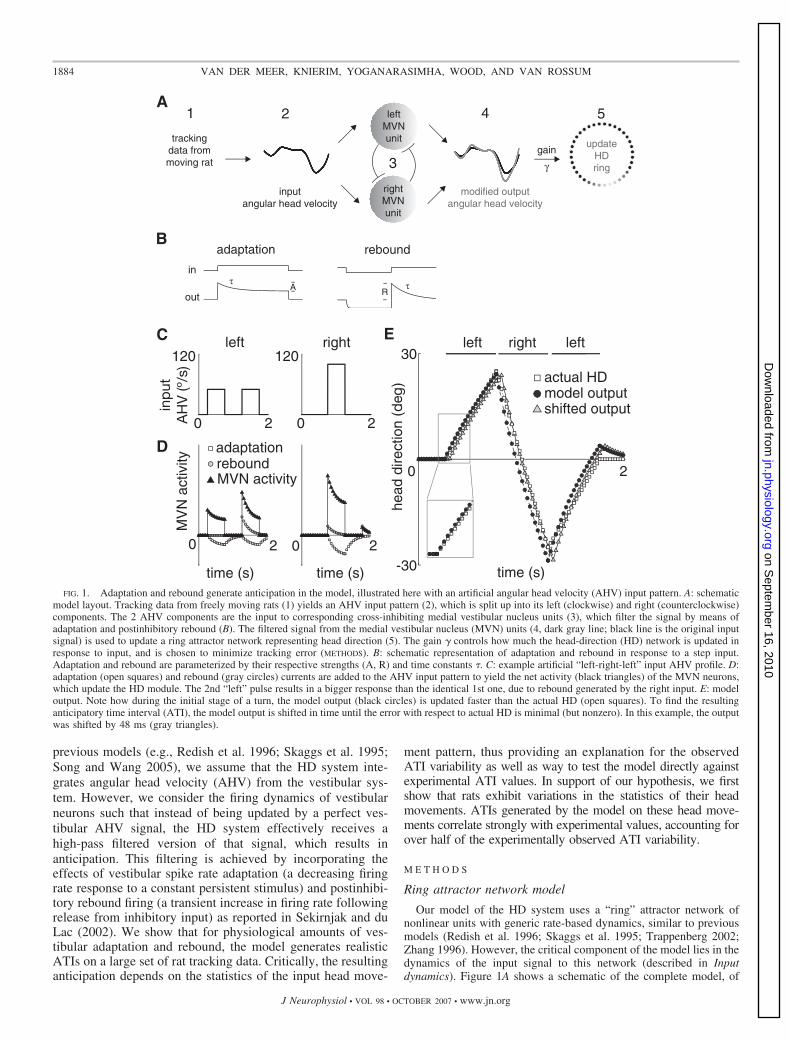
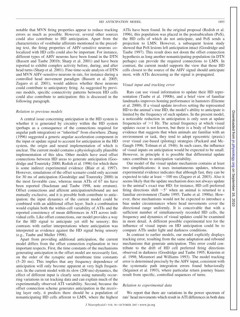
FIG. 1. Adaptation and rebound generate anticipation in the model, illustrated here with an artificial angular head velocity (AHV) input pattern. A: schematicmodel layout. Tracking data from freely moving rats (1) yields an AHV input pattern (2), which is split up into its left (clockwise) and right (counterclockwise)components. The 2 AHV components are the input to corresponding cross-inhibiting medial vestibular nucleus units (3), which filter the signal by means ofadaptation and postinhibitory rebound (B). The filtered signal from the medial vestibular nucleus (MVN) units (4, dark gray line; black line is the original inputsignal) is used to update a ring attractor network representing head direction (5). The gain � controls how much the head-direction (HD) network is updated inresponse to input, and is chosen to minimize tracking error (METHODS). B: schematic representation of adaptation and rebound in response to a step input.Adaptation and rebound are parameterized by their respective strengths (A, R) and time constants �. C: example artificial “left-right-left” input AHV profile. D:adaptation (open squares) and rebound (gray circles) currents are added to the AHV input pattern to yield the net activity (black triangles) of the MVN neurons,which update the HD module. The 2nd “left” pulse results in a bigger response than the identical 1st one, due to rebound generated by the right input. E: modeloutput. Note how during the initial stage of a turn, the model output (black circles) is updated faster than the actual HD (open squares). To find the resultinganticipatory time interval (ATI), the model output is shifted in time until the error with respect to actual HD is minimal (but nonzero). In this example, the outputwas shifted by 48 ms (gray triangles).

1884 VAN DER MEER, KNIERIM, YOGANARASIMHA, WOOD, AND VAN ROSSUM

J Neurophysiol • VOL 98 • OCTOBER 2007 • www.jn.org

on Septem

ber 16, 2010 jn.physiology.org

Dow

nloaded from

which the ring attractor network is the last processing stage. Ingeneral, like previous models, the ring network integrates AHV inputto yield a persistent representation of HD. Briefly, the network units(representing populations of neurons) are placed on a ring, whereangular position on the ring corresponds to the unit’s preferred firingdirection. A rotationally symmetric matrix of recurrent weights isconstructed so that a subset of units is persistently active, forming aGaussian-shaped activity packet, or attractor state, even in the absenceof input (Amari 1977). The packet is stable at any position along thering, and its position corresponds to the HD encoded by the network.The packet is moved around the ring by external inputs throughaddition of an asymmetric component to the weight matrix propor-tional to the magnitude of the input (Zhang 1996).

Specifically, following Stringer et al. (2002), the activity level u(t)of unit i in the HD ring is modeled by

�dui�t�

dt� �ui�t)��

j

wij(t)F[uj(t)]

where � is the time-constant of the unit and the activation function Fis a sigmoid

F�u� � 1/�1 � e��u)

with a slope denoted by �. The weight matrix w of the recurrentconnections in the network consists of a constant symmetric compo-nent ws, and two variable asymmetric components w{l,r}

a , which movethe activity packet left (clockwise) and right (counterclockwise),respectively.

w�t� � ws � ��vl�t)wla�vr�t)wr

a� (1)

The symmetric weight matrix ws implements a standard local excita-tion and global inhibition connectivity. The strength of the recurrentexcitation depends on the difference angle between the preferreddirections of the units

wijs � wEe

�dij2

2�2 � wI (2)

where dij is the angular difference between the preferred firingdirections of the units i, j; � denotes the width of the Gaussian weightprofile, and wE and wI determine the strength of the excitation andinhibition, respectively. These are chosen such that the network has astable attractor state.

The asymmetric components in Eq. 1 are obtained by multiplyingthe asymmetric weight profiles w{l,r}

a with the activity of the vestib-ular inputs v{l,r} and a constant gain (scaling) factor � (see sectionInput dynamics). For the asymmetric weights w{l,r}

a , we use thederivative of the symmetric weights given by Eq. 2, as in previousmodels (Stringer et al. 2002; Zhang 1996)

�wla�ij �

dij

�2 e�dij

2

2�2

for the left-turning weights and wra � �wl

a for the right-turningweights.

In summary, rotation of HD is effectively implemented through amodulation of the weights. We chose this simple implementationbecause the details of the update mechanism are not relevant for thisstudy, and the actual biological mechanism is not known, althoughmore detailed, biologically plausible, update mechanisms have beensuggested (Boucheny et al. 2005; Compte et al. 2000; Goodridge andTouretzky 2000; Song and Wang 2005).

Visual input

The attractor network described above provides a way for the HDrepresentation to be updated by idiothetic (self-motion) informationfrom the vestibular system. However, the HD system can also beupdated by visual information (Blair and Sharp 1996; Goodridge andTaube 1995; Taube et al. 1990b; Zugaro et al. 2003). Such visual“fixes,” where the animal uses visual cues in the environment to set itsHD representation, could affect anticipation. To quantify this, wemodel visual fixes as an instantaneous resetting of the HD represen-tation in the network to the animal’s actual HD. Specifically, at thetime of a fix, the activity packet is uniformly moved such that theabsolute angular difference between the model and actual HD isminimized.

Input dynamics

The core of the model describes how the input units that update theHD representation respond to the AHV �(t) to be tracked by themodel. The AHV signal is split up into “left” and “right” components,which feed into cross-inhibiting left (vl ) and right (vr ) units, consis-tent with vestibular system physiology (Markham et al. 1978;Shimazu and Precht 1966). These units correspond to a population ofAHV-sensitive neurons afferent to the HD system (see DISCUSSION).The firing properties of the input units are augmented with adaptationand rebound firing, as described in MVN neurons by Sekirnjak and duLac (2002); for clarity, we refer to the input units as “MVN units”.This arrangement is shown schematically in Fig. 1A. MVN unitactivity equals the AHV minus an adaptation current (IA), plus arebound current (IR), as follows

vr(t) � ��r�t) � I Ar �t� � I R

r �t� � vl�t)]� (3)

vl�t� � ��l�t� � I Al �t� � I R

l �t� � vr�t���

The last term describes vestibular cross-inhibition from the contralat-eral MVN unit. The angular velocity inputs �l(t) [and �r(t)] aresimply the right (left) components of the input angular velocity signal,i.e., �l(t) � [�(t)]� and �r(t) � [��(t)]�, where [x]� � max(x,0).

Prolonged activation of a MVN unit activates an adaptive currentIA, illustrated in Fig. 1B. The adaptive current is linear in the AHVinput and is modeled with a first-order differential equation. For theleft unit

�A

dI Al

dt� �IA

l � A�l�t) (4)

and similar for the right unit. The parameter �A describes the timeconstant of the adaptation build-up, and the parameter A denotes theadaptation strength. The adaptation current was chosen to depend onthe input rather than the activity of the unit itself to allow straight-forward interpretation of the parameter A as a fraction of the input, in

TABLE 1. Model parameters used for the results presented, unlessstated otherwise

Symbol Parameter Value

� Single unit time constant 10 ms�A Input adaptation current time constant 200 ms�R Input rebound current time constant 200 msdt Simulation time step 1 msN Number of neurons in ring 100� Activation function slope 0.07wE Recurrent weights scale factor 15� Recurrent weight profile width 21.6 degwI Recurrent weights global inhibition level 9A MVN unit adaption 0.4R MVN unit rebound 0.4

1885HD ANTICIPATION MODEL

J Neurophysiol • VOL 98 • OCTOBER 2007 • www.jn.org

on Septem

ber 16, 2010 jn.physiology.org

Dow

nloaded from

line with Sekirnjak and du Lac (2002). This does not change thequalitative features of the model. A parameter value A � 0 corre-sponds to no adaptation and A � 0.4 to a steady-state firing rate of60% of initial activity.

The postinhibitory rebound currents IRl (and IR

r , illustrated in Fig.1B) build up due to cross-inhibition from the contralateral side. Therebound current has a time constant �R and a net rebound gain factorR, which combines the strength of the contralateral inhibition andamount of rebound of the MVN unit

�R

I Rl

dt� �I R

l � R�r(t) (5)

and vice versa for IRr . Thus R � 0.2 means that when the left input ceases

to be active after a long time of activity (t �� �R), the right MVN unitrebounds with an initial activity level of 20% of the left input (cf. Eq. 3).For shorter rotation times, the rebound current is less. In Fig. 1, theadaptation and rebound currents are shown for a simple velocity profile.

Choice of parameters

For all simulations, we used A � R � 0.4 and �A � �R � 200 msunless stated otherwise. A � 0.4 corresponds to a strongly adaptingMVN neuron in Sekirnjak and du Lac (2002). The time constants wereextracted from a single-exponential fit to the published data. Thephysiological value of R is more difficult to estimate using currentlyavailable data because it depends on both the characteristics of theMVN neuron and on the strength of the cross-inhibition it receives.

To assess the effect of the simplifications and parameter choices ofour input implementation, we also simulated the MVN units v usingthe two conductance-based spiking MVN neuron models described inSekirnjak and du Lac (2002). Although we were unable to exactlyreproduce background firing rate of the reported model, the ratedynamics matched closely those reported there. To accommodatethese neuron models into our HD network, the left model neuronreceived excitatory input current proportional to �l and inhibitoryinput proportional to �r (and vice versa for the otherwise identicalright model neuron). The neurons’ spiking output was convolved witha Gaussian of 100 ms SD to serve as input v to our rate model. As theprecise proportionality between AHV and input current is not known,we have chosen values which make use of the full dynamic range ofthe neurons: we used 100 nA s/° (i.e., the instantaneous net inputcurrent to the neuron is 100 nA per unit angular velocity, which is indegrees per second) for excitation and 1,000 nA s/° for inhibition.This corresponds to strong inhibition and thus strong rebound; hence,the rebound simulation results should be viewed as an upper bound onhow much anticipation this mechanism generates.

Computing ATIs

The HD encoded by the model is extracted using a linear populationvector read-out (the vector sum of the preferred firing directions of themodel cells weighted by their firing rate) (Georgopoulos et al. 1982).To accurately track AHV input, the gain � needs to be set. The gaindetermines by how much the HD representation is updated in responseto a given input. An incorrect gain value leads to build-up of error inthe HD representation over time and can lead to artifactual anticipa-tion or lag. For each HD input profile [e.g., a 60-s segment of trackingdata (see following text), or an artificial step pattern], the optimal gainis found by minimizing the error between the model’s populationvector output and the time-shifted actual HD. The error is defined asthe summed absolute difference per second between input pattern anddecoded model output; using a sum of squares error yielded compa-rable results on a representative subset of the data. Both gain and timeshift were varied to minimize the error; the time shift correspondingto the minimal error output is the ATI for that pattern. To assess theeffect of computing the gain for each input separately, we also ran the

model on the set of tracking data with a fixed gain equal to the meangain previously obtained for each input pattern separately using theerror-minimizing procedure described in the preceding text. MeanATI values obtained this way did not differ significantly from thevalues reported, although both tracking error and ATI variability werehigher.

Using the model’s population vector output to compute ATIs ismuch more precise than the single-cell-based method used in theexperimental literature because all units in the model are accessible.To obtain the ATI of single cells in the model, the time shift whichmaximized the mutual information between the cell’s activity and theHD input was calculated, as was done for HD recording data (Taubeand Muller 1998).

Poisson HD cell simulation

To assess the anticipation variability that can be expected fromspiking variability alone (Fig. 3C), we used the fact that HD cell firingis thought to be approximately Poisson (Blair et al. 1998). Wesimulated a Poisson HD cell where the probability of a spike at eachsimulation time step (1 ms) was defined by a Gaussian tuning curve(� � 21°) for direction, with the mean 5° different for clockwiseversus counterclockwise turns respectively, to generate anticipation.The cell has a 100-Hz peak firing rate, 20-Hz mean firing rate, and 40ms of anticipation on average. The simulation used a 0.1-Hz sinusoi-dal directional profile 8 min in length, covering the entire directionalrange. For comparison with the experimental data from Blair et al.(1997), we used their method for computing ATIs in this simulation:two tuning curves for clockwise and counterclockwise turns wereconstructed, and the HD cell spikes were shifted in time until the twocurves overlap (Blair and Sharp 1995).

Tracking data

To provide the model with realistic inputs, rat HD tracking datawere used. Tracking data were obtained from adult male Long-Evans rats (n � 3) running a plus maze 1.8 m in diameter duringthe Neural Systems and Behavior summer course at the MarineBiological Laboratory, Woods Hole, MA. A color camera mountedoverhead sampled the light-emitting diode (LED) pattern of aHS-54 recording headstage (Neuralynx, Tucson, AZ) and a 10-cm-long boom attached to the rats’ head at 30Hz, as described inYoganarasimha et al. (2006). The effect of missing samples wasminimized first by only accepting recording sessions where 90%of the tracking samples were sufficient to determine instantaneousHD at the sampling points and second by extracting AHV frompairs of consecutive nonmissing samples only and using those toreconstruct a continuous HD profile. In other words, only AHVinformation known to sampling precision was used. This procedureleft 2 h and 22 min of usable data.

Because rat HD movements are sampled with finite precision and attoo coarse a time scale to be used as model inputs directly, weapproximated the rat’s true HD profile by fitting three different cubicsplines to each dataset: a spline that is forced to pass through allsampled points (natural or variational spline; no smoothing), as wellas a “weak” and a “strong” smoothing spline (MATLAB SplineToolbox function spaps, tolerances 0.001 and 0.002, respectively),which need not pass through every sample but are constrained by anerror function instead. The type of smoothing/interpolation applied tothe data slightly affects the absolute ATIs reported here but not thequalitative pattern of the results. All simulations are done on theweakly smoothed data.

We randomly selected 100 2-s- and 30 nonoverlapping 60-s-longsegments that had a mean absolute angular velocity between 45 and1,000°/s. The same set of 60-s segments was used for all tracking datasimulations except for the spiking models from Sekirnjak and du Lac(2002), for which the 2-s set was used to reduce simulation time. The

1886 VAN DER MEER, KNIERIM, YOGANARASIMHA, WOOD, AND VAN ROSSUM

J Neurophysiol • VOL 98 • OCTOBER 2007 • www.jn.org

on Septem

ber 16, 2010 jn.physiology.org

Dow

nloaded from

mean SD absolute AHV was 86.4 8.5°/s on the 60-s data(smallest: 67.0°/s, largest: 97.9°/s) and 100.5 29.3°/s on the 2-s data(smallest: 49.6°/s, largest: 179.6°/s). All input tracking data werearbitrarily assumed to start at zero HD; that is, the activity packet wasalways initialized at the same point in the ring. Because of therotational symmetry of the system, this does not affect the generalityof the results.

Experimental anticipation data

To compare the model’s predictions directly to experimental HDcell data, we used two recording data sets from two different behav-ioral tasks. The first set is a subset of the data described in Yoga-narasimha et al. (2006). Rats ran on an elevated circular track whileHD cell activity from the anterodorsal thalamic nucleus (ADN) wasrecorded and their head movements tracked. We used the “baseline”sessions, where apparatus and cues are always in the same, stableconfiguration. The second set is of rats foraging for randomly scat-tered chocolate sprinkles in a walled square box with a prominentpolarizing cue card, using the same recording procedure. This exper-iment is similar to recording conditions in previously reported HDanticipation data. A smoothing spline was fitted to the tracking data asin the preceding text.

The first “circular track” dataset included 12 3- to 6-min-longrecording sessions from a total of two animals, the second “squarebox” set consisted of 9 9- to 12-min-long sessions from three animals(1 of which also contributed to the circle dataset). In one animal in thesquare box data set, the recording electrode was identified as being inthe anteroventral thalamus (in the border region between the AV andVA nuclei). Data from this animal did not appear different in firing oranticipation properties and were therefore included. Every recordingsession was split up into 60-s segments, such that segment 1 for thatsession was the first 60 s, segment 2 the second 60 s, and so on. TheATI for each segment was then computed using the mutual informa-tion method described in Taube and Muller (1998). Segments �45 slong, or containing �400 spikes from a HD cell, were rejected. Forcomparison with model output, when multiple cells were recordedsimultaneously during a segment, the experimental ATI was taken tobe the mean of individual cells’ ATIs. ATIs for complete recording

sessions were obtained by averaging across the segments of thatsession.

R E S U L T S

We implement a single-layer continuous “ring” attractornetwork model of the rodent HD system, similar to previousmodels (Boucheny et al. 2005; Goodridge and Touretzky 2000;Redish et al. 1996; Song and Wang 2005; Stringer et al. 2002;Xie et al. 2002; Zhang 1996). This type of model has acontinuum of stable states in which a subset of HD cellsrepresenting the animal’s current directional heading is persis-tently active. To track the animal’s movement, the position ofthe packet needs to be updated. In contrast to earlier modelsand in accordance with physiology, we incorporate spike rateadaptation and postinhibitory rebound of MVN neurons(Sekirnjak and du Lac 2002) (Fig. 1B) into the update mech-anism. MVN neurons are thought to provide the vestibularinput to the HD system (Stackman and Taube 1997). As aresult, the input signal integrated by the model HD network isa modified version of the actual AHV. Following vestibularanatomy (Markham et al. 1978; Shimazu and Precht 1966), themodel contains left and right input units, the activity of whichprovides the update signal for the HD “ring.” These units,representing populations of MVN neurons, increase their ac-tivity during a left and a right turn, respectively. They adapt inresponse to constant input and cross-inhibit each other, result-ing in postinhibitory rebound when a turn stops and inhibitionis released. Adaptation and rebound are characterized by theirstrengths (A, R) and time constants (�A, �R); we fitted these tothe data in Sekirnjak and du Lac (2002) (METHODS). A sche-matic diagram of the model layout is shown in Fig. 1A.

The effect of MVN adaptation and rebound on our modelHD system is illustrated in Fig. 1, C–E, where a model ratmoves its head in an artificial left-right-left pattern. The AHVinput to be tracked by the model is first split up into left

100

101

102

103

0

40

80

120

160

200

AHV (deg/s)

AT

I (m

s)

-A-R+A-R-A+R+A+R

10

40

80

120

160

200

input frequency (Hz)

-A-R+A-R-A+R+A+R

AH

V

AH

V

A B

0.1 5

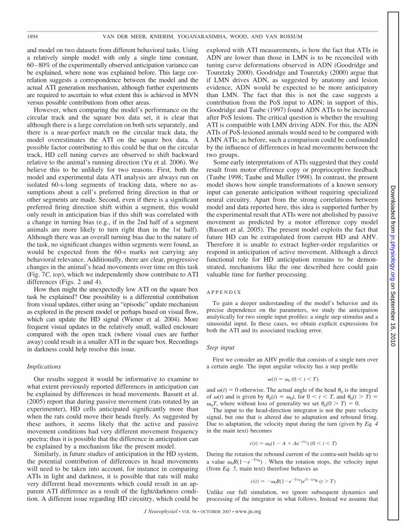
FIG. 2. Anticipation in the model depends on input frequency but not on input magnitude. A: ATI as a function of AHV using a step input. Adaptation (A)and rebound (R) can both generate anticipation independently (�A�R/gray diamonds and �A�R/gray triangles, respectively), and add supralinearly(�A�R/black squares). B: ATI as a function of frequency of a sinusoidal input. Higher input frequencies result in less anticipation. At low frequencies, adaptationgenerates more anticipation than rebound. For analytical results supporting these simulations, see the APPENDIX. The step input patterns were 6 s long: 1 s ofconstant input followed by 5 s of rest. The sinusoidal input patterns were 10 s long, the ATI was computed over the last 5 s to eliminate the effects of initialtransients. Parameters in METHODS.

1887HD ANTICIPATION MODEL

J Neurophysiol • VOL 98 • OCTOBER 2007 • www.jn.org

on Septem

ber 16, 2010 jn.physiology.org

Dow

nloaded from

(clockwise) and right (counterclockwise) components (Fig.1C). This input is then modified by adaptation (Fig. 1D, opensquares) and rebound currents (Fig. 1D, gray circles) to yieldthe net MVN activity (Fig. 1D, black triangles). Specifically,the left MVN unit responds to the constant leftward input andadapts, whereas rebound current builds up in the right MVNunit. The rebound becomes active once left movement stops(releasing cross-inhibition), coinciding with the start of theright turn. The right MVN response to the right turn is boostedby the rebound current. Meanwhile, as the right unit adapts,rebound builds up in the left MVN unit. This rebound thenboosts the response to the following left turn: compare theresponse to the two identical turns in the left MVN unit. Thesecond response is larger due to the rebound current generatedby the intervening right turn.

The net activity of the left and right MVN units described inthe preceding text moves the HD representation in the corre-sponding direction, allowing the system to track a given inputpattern. Exactly how much the HD activity packet moves inresponse to MVN activity is determined by a fixed gainparameter �, which is chosen to minimize tracking error(METHODS). For our example, the model’s resulting HD repre-

sentation can be seen in Fig. 1E. As the movement stimulusstarts, the model output (black circles) initially updates fasterthan the actual HD (open squares). When the stimulus changesdirection, rebound provides an additional update boost. Thesemechanisms effectively implement a high-pass filter or angularacceleration component (Song and Wang 2005; Zhang 1996),although it cannot simply be described as a linear filter (see theAPPENDIX). The result is anticipation: the model output precedesthe actual HD in time. To calculate by how much the modelanticipates, the model output is shifted in time to minimize theerror with respect to the actual HD (METHODS). The time shiftcorresponding to the minimal error (gray triangles in Fig. 1E)is the model’s ATI. For this example, the model’s ATI was 48ms.

Anticipation on artificial input patterns

To characterize the model’s behavior further, we firstpresent simple artificial AHV patterns to the model. On stepinputs of constant AHV (Fig. 2A), adaptation only (�A�R)and rebound only (�A�R) both generate anticipation. Whenadaptation and rebound are combined (�A�R), the resulting

0 0.1 0.2 0.3 0.40

20

40

60

80

100

120

adaptation

AT

I (m

s)

rebound = 0rebound = 0.4rebound = 0.8

+A-R +A+R -A-R0

20

40

60

80

100

120

AT

I (m

s)

neuron Aneuron B

AT

I std

. dev

. (m

s)

A B

C D

adaptation

rebo

und

0 0.1 0.2 0.3 0.40

0.1

0.2

0.3

0.4

0.1

0.15

0.2

0.25

0.3+

error (deg/s) per ms anticipation

simul.Poisson

0

5

10

15

20

model-A-R

model+A+R

dataall

datawithin

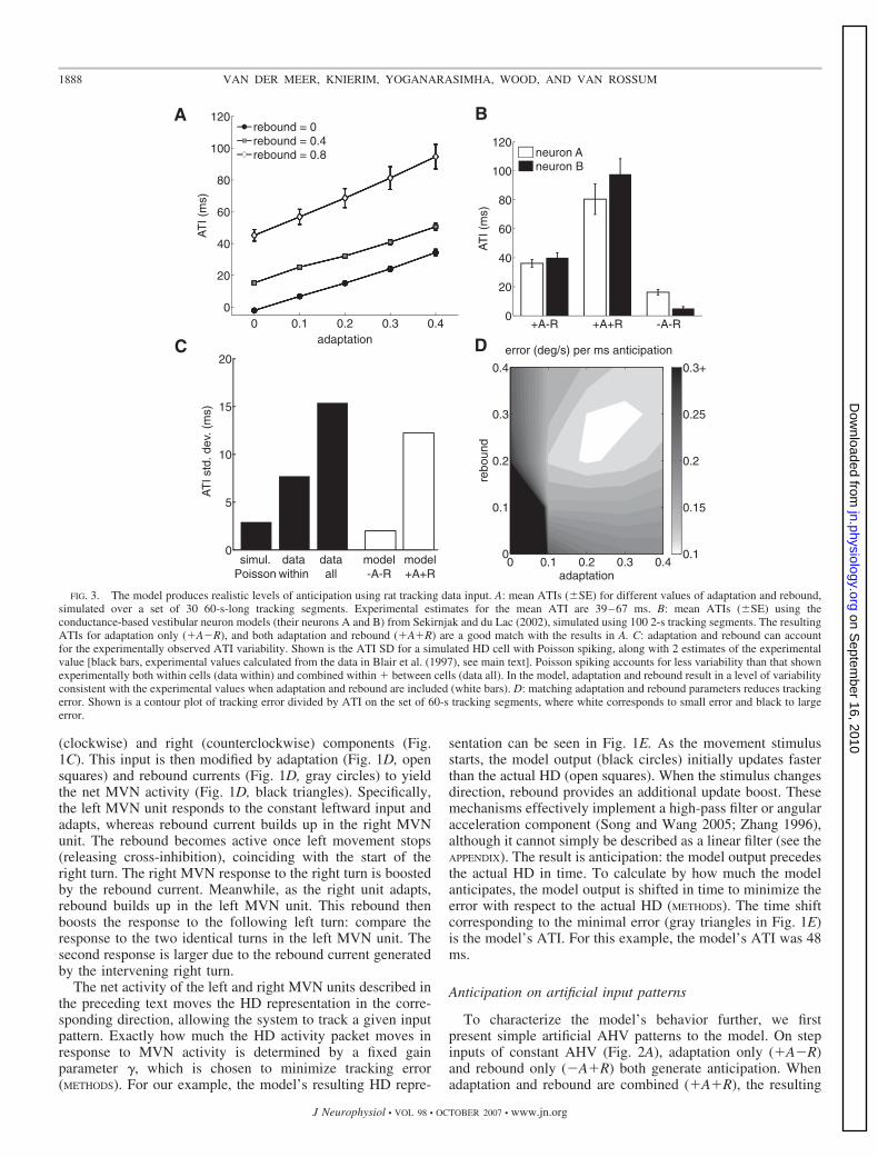
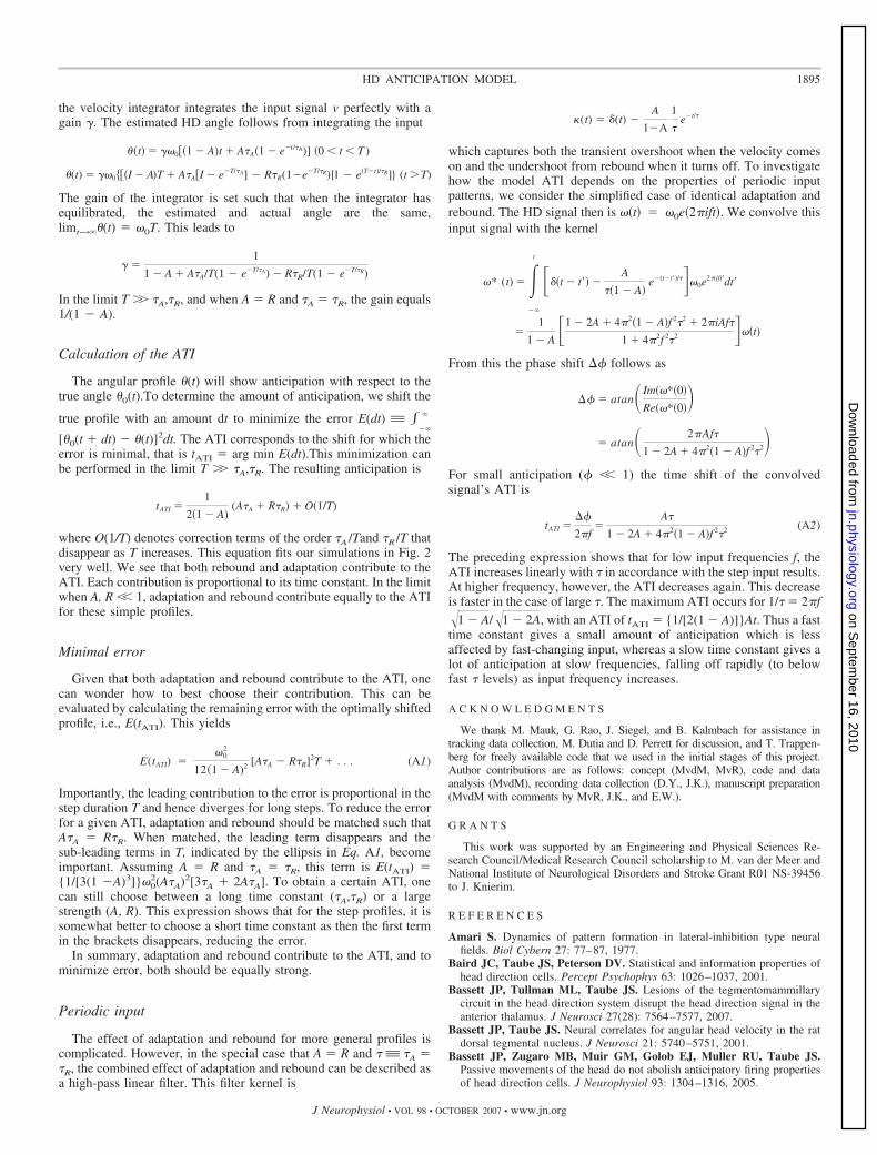
FIG. 3. The model produces realistic levels of anticipation using rat tracking data input. A: mean ATIs (SE) for different values of adaptation and rebound,simulated over a set of 30 60-s-long tracking segments. Experimental estimates for the mean ATI are 39–67 ms. B: mean ATIs (SE) using theconductance-based vestibular neuron models (their neurons A and B) from Sekirnjak and du Lac (2002), simulated using 100 2-s tracking segments. The resultingATIs for adaptation only (�A�R), and both adaptation and rebound (�A�R) are a good match with the results in A. C: adaptation and rebound can accountfor the experimentally observed ATI variability. Shown is the ATI SD for a simulated HD cell with Poisson spiking, along with 2 estimates of the experimentalvalue [black bars, experimental values calculated from the data in Blair et al. (1997), see main text]. Poisson spiking accounts for less variability than that shownexperimentally both within cells (data within) and combined within � between cells (data all). In the model, adaptation and rebound result in a level of variabilityconsistent with the experimental values when adaptation and rebound are included (white bars). D: matching adaptation and rebound parameters reduces trackingerror. Shown is a contour plot of tracking error divided by ATI on the set of 60-s tracking segments, where white corresponds to small error and black to largeerror.

1888 VAN DER MEER, KNIERIM, YOGANARASIMHA, WOOD, AND VAN ROSSUM

J Neurophysiol • VOL 98 • OCTOBER 2007 • www.jn.org

on Septem

ber 16, 2010 jn.physiology.org

Dow

nloaded from

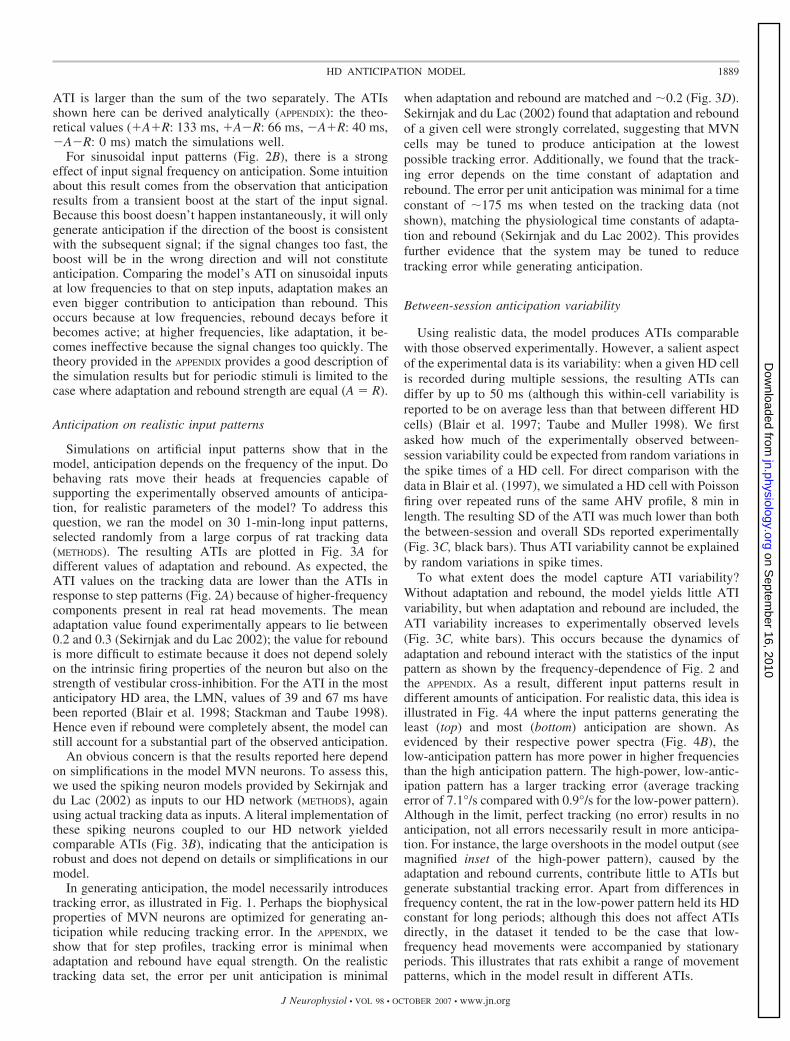
ATI is larger than the sum of the two separately. The ATIsshown here can be derived analytically (APPENDIX): the theo-retical values (�A�R: 133 ms, �A�R: 66 ms, �A�R: 40 ms,�A�R: 0 ms) match the simulations well.

For sinusoidal input patterns (Fig. 2B), there is a strongeffect of input signal frequency on anticipation. Some intuitionabout this result comes from the observation that anticipationresults from a transient boost at the start of the input signal.Because this boost doesn’t happen instantaneously, it will onlygenerate anticipation if the direction of the boost is consistentwith the subsequent signal; if the signal changes too fast, theboost will be in the wrong direction and will not constituteanticipation. Comparing the model’s ATI on sinusoidal inputsat low frequencies to that on step inputs, adaptation makes aneven bigger contribution to anticipation than rebound. Thisoccurs because at low frequencies, rebound decays before itbecomes active; at higher frequencies, like adaptation, it be-comes ineffective because the signal changes too quickly. Thetheory provided in the APPENDIX provides a good description ofthe simulation results but for periodic stimuli is limited to thecase where adaptation and rebound strength are equal (A � R).

Anticipation on realistic input patterns

Simulations on artificial input patterns show that in themodel, anticipation depends on the frequency of the input. Dobehaving rats move their heads at frequencies capable ofsupporting the experimentally observed amounts of anticipa-tion, for realistic parameters of the model? To address thisquestion, we ran the model on 30 1-min-long input patterns,selected randomly from a large corpus of rat tracking data(METHODS). The resulting ATIs are plotted in Fig. 3A fordifferent values of adaptation and rebound. As expected, theATI values on the tracking data are lower than the ATIs inresponse to step patterns (Fig. 2A) because of higher-frequencycomponents present in real rat head movements. The meanadaptation value found experimentally appears to lie between0.2 and 0.3 (Sekirnjak and du Lac 2002); the value for reboundis more difficult to estimate because it does not depend solelyon the intrinsic firing properties of the neuron but also on thestrength of vestibular cross-inhibition. For the ATI in the mostanticipatory HD area, the LMN, values of 39 and 67 ms havebeen reported (Blair et al. 1998; Stackman and Taube 1998).Hence even if rebound were completely absent, the model canstill account for a substantial part of the observed anticipation.

An obvious concern is that the results reported here dependon simplifications in the model MVN neurons. To assess this,we used the spiking neuron models provided by Sekirnjak anddu Lac (2002) as inputs to our HD network (METHODS), againusing actual tracking data as inputs. A literal implementation ofthese spiking neurons coupled to our HD network yieldedcomparable ATIs (Fig. 3B), indicating that the anticipation isrobust and does not depend on details or simplifications in ourmodel.

In generating anticipation, the model necessarily introducestracking error, as illustrated in Fig. 1. Perhaps the biophysicalproperties of MVN neurons are optimized for generating an-ticipation while reducing tracking error. In the APPENDIX, weshow that for step profiles, tracking error is minimal whenadaptation and rebound have equal strength. On the realistictracking data set, the error per unit anticipation is minimal

when adaptation and rebound are matched and 0.2 (Fig. 3D).Sekirnjak and du Lac (2002) found that adaptation and reboundof a given cell were strongly correlated, suggesting that MVNcells may be tuned to produce anticipation at the lowestpossible tracking error. Additionally, we found that the track-ing error depends on the time constant of adaptation andrebound. The error per unit anticipation was minimal for a timeconstant of 175 ms when tested on the tracking data (notshown), matching the physiological time constants of adapta-tion and rebound (Sekirnjak and du Lac 2002). This providesfurther evidence that the system may be tuned to reducetracking error while generating anticipation.

Between-session anticipation variability

Using realistic data, the model produces ATIs comparablewith those observed experimentally. However, a salient aspectof the experimental data is its variability: when a given HD cellis recorded during multiple sessions, the resulting ATIs candiffer by up to 50 ms (although this within-cell variability isreported to be on average less than that between different HDcells) (Blair et al. 1997; Taube and Muller 1998). We firstasked how much of the experimentally observed between-session variability could be expected from random variations inthe spike times of a HD cell. For direct comparison with thedata in Blair et al. (1997), we simulated a HD cell with Poissonfiring over repeated runs of the same AHV profile, 8 min inlength. The resulting SD of the ATI was much lower than boththe between-session and overall SDs reported experimentally(Fig. 3C, black bars). Thus ATI variability cannot be explainedby random variations in spike times.

To what extent does the model capture ATI variability?Without adaptation and rebound, the model yields little ATIvariability, but when adaptation and rebound are included, theATI variability increases to experimentally observed levels(Fig. 3C, white bars). This occurs because the dynamics ofadaptation and rebound interact with the statistics of the inputpattern as shown by the frequency-dependence of Fig. 2 andthe APPENDIX. As a result, different input patterns result indifferent amounts of anticipation. For realistic data, this idea isillustrated in Fig. 4A where the input patterns generating theleast (top) and most (bottom) anticipation are shown. Asevidenced by their respective power spectra (Fig. 4B), thelow-anticipation pattern has more power in higher frequenciesthan the high anticipation pattern. The high-power, low-antic-ipation pattern has a larger tracking error (average trackingerror of 7.1°/s compared with 0.9°/s for the low-power pattern).Although in the limit, perfect tracking (no error) results in noanticipation, not all errors necessarily result in more anticipa-tion. For instance, the large overshoots in the model output (seemagnified inset of the high-power pattern), caused by theadaptation and rebound currents, contribute little to ATIs butgenerate substantial tracking error. Apart from differences infrequency content, the rat in the low-power pattern held its HDconstant for long periods; although this does not affect ATIsdirectly, in the dataset it tended to be the case that low-frequency head movements were accompanied by stationaryperiods. This illustrates that rats exhibit a range of movementpatterns, which in the model result in different ATIs.

1889HD ANTICIPATION MODEL

J Neurophysiol • VOL 98 • OCTOBER 2007 • www.jn.org

on Septem

ber 16, 2010 jn.physiology.org

Dow

nloaded from

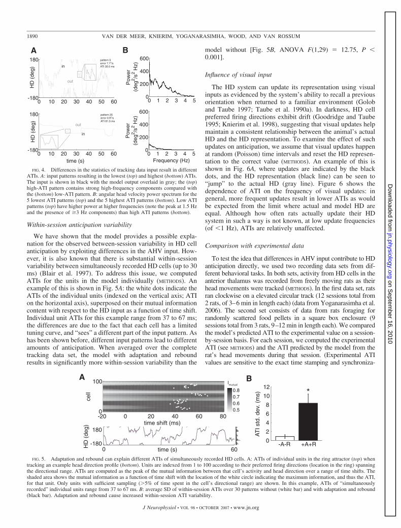
Within-session anticipation variability

We have shown that the model provides a possible expla-nation for the observed between-session variability in HD cellanticipation by exploiting differences in the AHV input. How-ever, it is also known that there is substantial within-sessionvariability between simultaneously recorded HD cells (up to 30ms) (Blair et al. 1997). To address this issue, we computedATIs for the units in the model individually (METHODS). Anexample of this is shown in Fig. 5A: the white dots indicate theATIs of the individual units (indexed on the vertical axis; ATIon the horizontal axis), superposed on their mutual informationcontent with respect to the HD input as a function of time shift.Individual unit ATIs for this example range from 37 to 67 ms;the differences are due to the fact that each cell has a limitedtuning curve, and “sees” a different part of the input pattern. Ashas been shown before, different input patterns lead to differentamounts of anticipation. When averaged over the completetracking data set, the model with adaptation and reboundresults in significantly more within-session variability than the

model without [Fig. 5B, ANOVA F(1,29) � 12.75, P �0.001].

Influence of visual input

The HD system can update its representation using visualinputs as evidenced by the system’s ability to recall a previousorientation when returned to a familiar environment (Goloband Taube 1997; Taube et al. 1990a). In darkness, HD cellpreferred firing directions exhibit drift (Goodridge and Taube1995; Knierim et al. 1998), suggesting that visual updates helpmaintain a consistent relationship between the animal’s actualHD and the HD representation. To examine the effect of suchupdates on anticipation, we assume that visual updates happenat random (Poisson) time intervals and reset the HD represen-tation to the correct value (METHODS). An example of this isshown in Fig. 6A, where updates are indicated by the blackdots, and the HD representation (black line) can be seen to“jump” to the actual HD (gray line). Figure 6 shows thedependence of ATI on the frequency of visual updates: ingeneral, more frequent updates result in lower ATIs as wouldbe expected from the limit where actual and model HD areequal. Although how often rats actually update their HDsystem in such a way is not known, at low update frequencies(of �1 Hz), ATIs are relatively unaffected.

Comparison with experimental data

To test the idea that differences in AHV input contribute to HDanticipation directly, we used two recording data sets from dif-ferent behavioral tasks. In both sets, activity from HD cells in theanterior thalamus was recorded from freely moving rats as theirhead movements were tracked (METHODS). In the first data set, ratsran clockwise on a elevated circular track (12 sessions total from2 rats, of 3–6 min in length each) (data from Yoganarasimha et al.2006). The second set consists of data from rats foraging forrandomly scattered food pellets in a square box enclosure (9sessions total from 3 rats, 9–12 min in length each). We comparedthe model’s predicted ATI to the experimental value on a session-by-session basis. For each session, we computed the experimentalATI (see METHODS) and the ATI predicted by the model from therat’s head movements during that session. (Experimental ATIvalues are sensitive to the exact time stamping and synchroniza-

FIG. 4. Differences in the statistics of tracking data input result in differentATIs. A: input patterns resulting in the lowest (top) and highest (bottom) ATIs.The input is shown in black with the model output overlaid in gray; the (top)high-ATI pattern contains strong high-frequency components compared withthe (bottom) low-ATI pattern. B: angular head velocity power spectrum for the5 lowest ATI patterns (top) and the 5 highest ATI patterns (bottom). Low ATIpatterns (top) have higher power at higher frequencies (note the peak at 1.5 Hzand the presence of 3 Hz components) than high ATI patterns (bottom).

-20 0 20 40 60 80

100

time shift (ms)

cell

0 60-180

180

time (s)HD

(de

g)

0.50.60.70.8

-A-R +A+R0

2

4

6

8

10

12*

AT

I std

. dev

. (m

s)

BA

0

Imutual

FIG. 5. Adaptation and rebound can explain different ATIs of simultaneously recorded HD cells. A: ATIs of individual units in the ring attractor (top) whentracking an example head direction profile (bottom). Units are indexed from 1 to 100 according to their preferred firing directions (location in the ring) spanningthe directional range. ATIs are computed as the peak of the mutual information between that cell’s activity and head direction over a range of time shifts. Theshaded area shows the mutual information as a function of time shift with the location of the white circle indicating the maximum information, and thus the ATI,for that unit. Only units with sufficient sampling (�5% of time spent in the cell’s directional range) are shown. In this example, ATIs of “simultaneouslyrecorded” individual units range from 37 to 67 ms. B: average SD of within-session ATIs over 30 patterns without (white bar) and with adaptation and rebound(black bar). Adaptation and rebound cause increased within-session ATI variability.

1890 VAN DER MEER, KNIERIM, YOGANARASIMHA, WOOD, AND VAN ROSSUM

J Neurophysiol • VOL 98 • OCTOBER 2007 • www.jn.org

on Septem

ber 16, 2010 jn.physiology.org

Dow

nloaded from

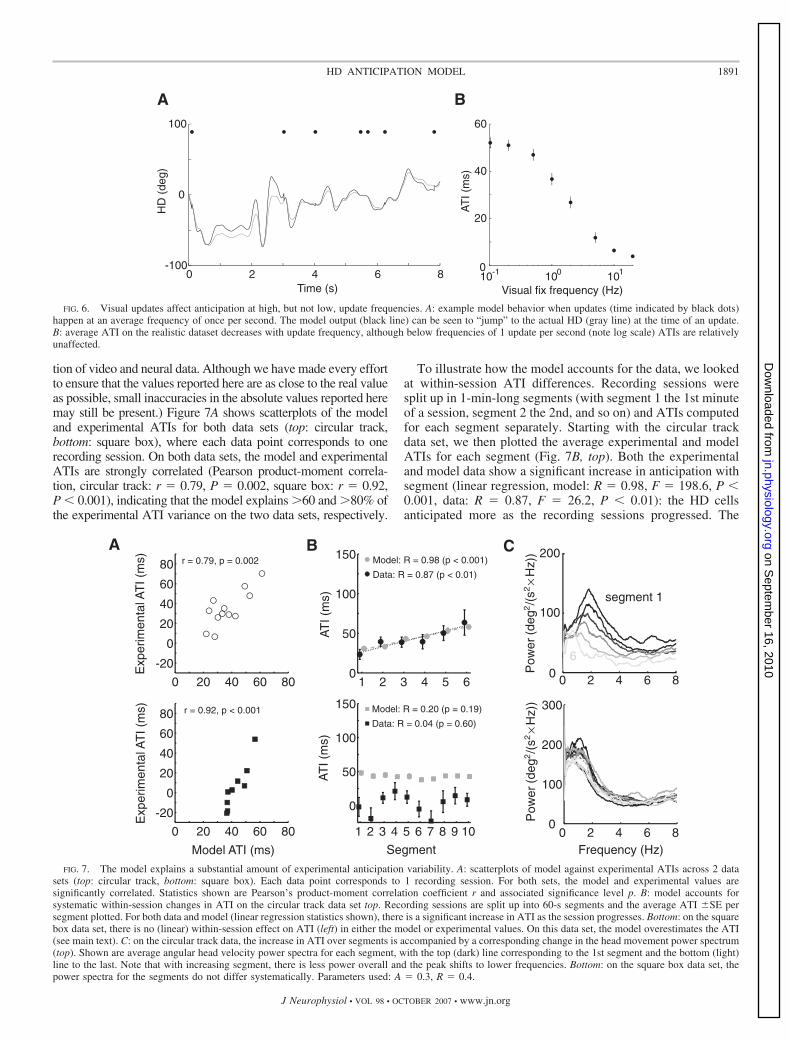
tion of video and neural data. Although we have made every effortto ensure that the values reported here are as close to the real valueas possible, small inaccuracies in the absolute values reported heremay still be present.) Figure 7A shows scatterplots of the modeland experimental ATIs for both data sets (top: circular track,bottom: square box), where each data point corresponds to onerecording session. On both data sets, the model and experimentalATIs are strongly correlated (Pearson product-moment correla-tion, circular track: r � 0.79, P � 0.002, square box: r � 0.92,P � 0.001), indicating that the model explains �60 and �80% ofthe experimental ATI variance on the two data sets, respectively.

To illustrate how the model accounts for the data, we lookedat within-session ATI differences. Recording sessions weresplit up in 1-min-long segments (with segment 1 the 1st minuteof a session, segment 2 the 2nd, and so on) and ATIs computedfor each segment separately. Starting with the circular trackdata set, we then plotted the average experimental and modelATIs for each segment (Fig. 7B, top). Both the experimentaland model data show a significant increase in anticipation withsegment (linear regression, model: R � 0.98, F � 198.6, P �0.001, data: R � 0.87, F � 26.2, P � 0.01): the HD cellsanticipated more as the recording sessions progressed. The

FIG. 6. Visual updates affect anticipation at high, but not low, update frequencies. A: example model behavior when updates (time indicated by black dots)happen at an average frequency of once per second. The model output (black line) can be seen to “jump” to the actual HD (gray line) at the time of an update.B: average ATI on the realistic dataset decreases with update frequency, although below frequencies of 1 update per second (note log scale) ATIs are relativelyunaffected.

B

AT

I (m

s)

0 2 4 6 80

100

200

Pow

er (d

eg2/(

s2 × H

z))

segment 1

6

A

Segment

AT

I (m

s)

0 2 4 6 8 0

100

200

300

Frequency (Hz)

Pow

er (d

eg2/(

s2 × H

z))

C

1 2 3 4 5 6 7 8 9 10

0

50

100

150

Model: R = 0.20 (p = 0.19)

Data: R = 0.04 (p = 0.60)

1 2 3 4 5 60

50

100

150

Model: R = 0.98 (p < 0.001)

Data: R = 0.87 (p < 0.01)

Model ATI (ms)

Exp

erim

enta

l AT

I (m

s) r = 0.79, p = 0.002

Exp

erim

enta

l AT

I (m

s) r = 0.92, p < 0.001

0 20 40 60 80

-20

0

20

40

60

80

0 20 40 60 80

-20

0

20

40

60

80

FIG. 7. The model explains a substantial amount of experimental anticipation variability. A: scatterplots of model against experimental ATIs across 2 datasets (top: circular track, bottom: square box). Each data point corresponds to 1 recording session. For both sets, the model and experimental values aresignificantly correlated. Statistics shown are Pearson’s product-moment correlation coefficient r and associated significance level p. B: model accounts forsystematic within-session changes in ATI on the circular track data set top. Recording sessions are split up into 60-s segments and the average ATI SE persegment plotted. For both data and model (linear regression statistics shown), there is a significant increase in ATI as the session progresses. Bottom: on the squarebox data set, there is no (linear) within-session effect on ATI (left) in either the model or experimental values. On this data set, the model overestimates the ATI(see main text). C: on the circular track data, the increase in ATI over segments is accompanied by a corresponding change in the head movement power spectrum(top). Shown are average angular head velocity power spectra for each segment, with the top (dark) line corresponding to the 1st segment and the bottom (light)line to the last. Note that with increasing segment, there is less power overall and the peak shifts to lower frequencies. Bottom: on the square box data set, thepower spectra for the segments do not differ systematically. Parameters used: A � 0.3, R � 0.4.

1891HD ANTICIPATION MODEL

J Neurophysiol • VOL 98 • OCTOBER 2007 • www.jn.org

on Septem

ber 16, 2010 jn.physiology.org

Dow

nloaded from

model explains this increase by changes in the frequencycontent of rat’s head movements. Average power spectra foreach segment are shown in Fig. 7C (top); the darkest linecorresponds to the first segment, with the line for each subse-quent segment colored progressively lighter. The first segment(top black line) has higher overall power and a peak at a higherfrequency than the last segment (bottom, light gray line). As inFigs. 2B and 4, higher frequency components result in lessanticipation in the model and in the recording data.

In contrast, the square box data set did not show an effect ofsegment on ATI for either model or experimental data (Fig. 7B,bottom; linear regression, model: R � 0.2, F � 2.0, P � 0.19;data: R � 0.04, F � 1.3, P � 0.60). Consistent with this, theaverage power spectra per segment (Fig. 7, bottom) do notshow a clear progression as in the circular track data set. AsFig. 7, A and B (bottom) illustrates, although there is a strongcorrelation between the model and the data, the model over-estimates the experimentally observed ATI on the square boxdata set in absolute terms and underestimates its modulation.The fact that the model does not always reproduce the exactATI values is not surprising. Apart from the potential influenceof different visual update frequencies (Fig. 6), the modelimplements a simplified view of AHV input signal processing.In modeling MVN adaptation and rebound with a singleexponential, it does not include contributions from mecha-nisms with different time constants (e.g., adaptation in thevestibular apparatus itself). Such contributions would respondto different components of the head movement power spec-trum, potentially contributing differences between differentdata sets not seen in the current implementation. Also severalexperimental factors beyond the scope of the model may affectabsolute ATI values, including the use of different subjects forthe two data sets or the walls of the square box environmentrestricting head movements artificially (e.g., the rat spendsmuch time searching for food pellets along the walls or in thecorners and thus does not have the freedom to move its head inall directions). In our view, the fact that the model can accountfor much of the experimentally observed anticipation varianceon both data sets without tuning of parameters is more com-pelling than if we had fit the parameters to the anticipation datawithout physiological justification or if we had invoked artifi-cial mechanisms to produce a better fit.

D I S C U S S I O N

We provide a novel hypothesis on how anticipation isgenerated in the HD system. Following the in vitro firingproperties of MVN neurons, which are thought to provideAHV information to the HD system, we incorporate physio-logical levels of adaptation and rebound firing in our model.The model produces realistic anticipation without further pa-rameter tuning when run on a corpus of rat tracking data. In themodel, the statistics of the rat’s head movements interact withthe high-pass filtering generated by adaptation and rebound,such that movement patterns with high-frequency componentsresult in lower anticipation than lower-frequency movements.We show that rats exhibit variations in the power spectrum oftheir head movements in the relevant frequency range. Whenthe model output is compared directly against experimentalrecording data from two different behavioral tasks, the modelaccounts for 60–80% of the experimentally observed variance,

although some differences between the two data sets remainunexplained. We conclude that the firing properties of neuronsafferent to the HD system, specifically their dynamic responseto head movements, may be important in generating HDanticipation. This idea has implications for our understandingof the circuitry of the HD system as it stands in contrast toprevious proposals that treat anticipation as a consequence ofcircuitry within the HD system. Furthermore, the result thatATIs depend on the statistics of head movements has method-ological implications for the study of ATIs.

Origin of the HD update signal

The present model uses the firing properties of neurons inthe MVN to generate anticipation in the HD system. Severallines of evidence indicate that the MVN are a likely origin ofvestibular inputs to the HD system (for a review, see Brown etal. 2002). Anatomically, the MVN project to the dorsal teg-mental nuclei of Gudden (DTN), through the nucleus preposi-tus hyperglossi (nPH) and possibly also directly (Brown et al.2005; Hayakawa and Zyo 1985; Liu et al. 1984). DTN, in turn,is reciprocally connected with the LMN (Gonzalo-Ruiz et al.1992). Both these areas contain AHV as well as HD cells, andcause loss of downstream directional firing when lesioned(Bassett et al. 2007; Blair et al. 1998; Sharp et al. 2001b).Similarly, bilateral lesions of the vestibular apparatus itselfabolish directional activity in HD areas (Stackman and Taube1997). Recording studies (albeit to our knowledge not in rats)have shown that semicircular canal-dependent MVN neuronalactivity contains AHV information (e.g., Fuchs and Kimm1975; Melvill Jones and Milsum 1971; Vidal and Sans 2004),which is theoretically sufficient to update the HD representa-tion. Thus given that the vestibular AHV signal appears to beresponsible for updating the HD system, its properties arerelevant to models of the HD system.

We based our model on the intrinsic firing properties ofMVN neurons (Sekirnjak and du Lac 2002) as reported in ratbrain slices. In recordings from intact animals, the MVNresponse is reported to have a phase lead relative to a sinusoi-dal AHV input (Fuchs and Kimm 1975; Melvill Jones andMilsum 1971; Vidal and Sans 2004), which decreases and evenlags with increasing frequency (Kaufman et al. 2000). Thispattern is consistent with our model. Although it is possiblethat this phase lead results from the properties of vestibularafferents (e.g., Fernandez and Goldberg 1971) rather than, or inaddition to, intrinsic MVN firing properties, our implementa-tion captures the relevant dynamics.

In principle, the model’s ability to generate anticipation onlydepends on the HD input signal being a high-pass filtered AHVsignal. More generally, any input signal that also contains atime-derivative component (in the HD system, AHV plus anacceleration component) will result in anticipation when inte-grated and decoded provided that the encoded quantity (HD)varies smoothly (Puccini et al. 2007). The neural mechanismsthat accomplish this in the HD system need not exclusively beimplemented in the MVN. Because the precise update circuit isnot yet known, we have concentrated on the possible contri-bution from the MVN for two reasons. First, it is a likelysource of input to the HD system as discussed in the precedingtext. Second, known physiological properties of MVN explaina large fraction of the observed ATI. In this respect, it is

1892 VAN DER MEER, KNIERIM, YOGANARASIMHA, WOOD, AND VAN ROSSUM

J Neurophysiol • VOL 98 • OCTOBER 2007 • www.jn.org

on Septem

ber 16, 2010 jn.physiology.org

Dow

nloaded from

notable that MVN firing properties appear to reduce trackingerrors as much as possible. However, several other sourcescould also contribute to HD anticipation. Apart from thecharacteristics of vestibular afferents mentioned in the preced-ing text, the firing properties of AHV-sensitive neurons co-localized with HD cells could also be important. For instance,different types of AHV neurons have been found in the DTN(Bassett and Taube 2001b; Sharp et al. 2001) and have beenreported to exhibit complex activity before, during, and afterhead turns (Sharp et al. 2001). Fine-time-scale analysis of DTNand MVN AHV-sensitive neurons in rats, for instance during acontrolled head movement paradigm (Bassett et al. 2005;Zugaro et al. 2001), would address whether these neuronscould contribute to anticipatory firing. As suggested by previ-ous models, specific connectivity patterns between HD cellscould also contribute to anticipation: this is discussed in thefollowing paragraph.

Relation to previous models

A central issue concerning anticipation in the HD system iswhether it is generated by circuitry within the HD system(perhaps as a consequence of the connections required forangular path integration) or “inherited” from elsewhere. Zhang(1996) suggested a generic angular acceleration component inthe input or update signal to account for anticipation in the HDsystem, the origin and neural implementation of which isunclear. The current model contains a physiologically plausibleimplementation of this idea. Other models have used offsetconnections between HD areas to generate anticipation (Goo-dridge and Touretzky 2000; Redish et al. 1996) for which thereis some indirect experimental evidence (Blair et al. 1997).However, simulations of the offset scenario could only accountfor 30 ms of anticipation (Goodridge and Touretzky 2000) inthe most favorable case, whereas mean ATIs of 67 ms havebeen reported (Stackman and Taube 1998, note erratum).Offset connections and afferent anticipation/rebound are notmutually exclusive, and it is possible both contribute to antic-ipation: the input dynamics of the current model could becombined with an additional offset layer. Such a combinationwould explain both the within-cell variability of ATIs and thereported consistency of mean differences in ATI across indi-vidual cells. Like offset connections, our model provides a wayfor the HD signal to anticipate yet still be sensory; thiscontrasts with earlier interpretations where anticipation wasinterpreted as evidence against the HD signal being sensory(e.g., Taube and Muller 1998).

Apart from providing additional anticipation, the currentmodel differs from the offset connection explanation in twoimportant respects. First, the time constants of the mechanismsgenerating anticipation in the offset model are necessarily fast,on the order of the synaptic and membrane time constants(5–20 ms). This implies that any frequency dependence ofanticipation will only become apparent at very high frequen-cies. In the current model with its slow (200 ms) dynamics, theeffect of different input is clearly seen using naturally occur-ring variations in rat tracking data and can explain much of theexperimentally observed ATI variability. Second, because theoffset connection scheme generates anticipation in the receiv-ing layer only, it predicts there should be a population ofnonanticipating HD cells afferent to LMN, where the highest

ATIs have been found. In the original proposal (Redish et al.1996), this population was placed in the postsubiculum (PoS),the HD cells of which do not anticipate, and PoS sends aprojection to LMN. However, a subsequent lesion studyshowed that PoS lesions left anticipation intact (Goodridge andTaube 1997). This result does not doom the offset connectionhypothesis as long another nonanticipating population (in DTNperhaps) can provide the required connections to LMN. Incontrast, the current model supports the view that those HDcells closest to the source of the AHV signal should anticipatemost, with ATIs decreasing as the signal is propagated.

Visual input and tracking error

Rats can use visual information to update their HD repre-sentation (Taube et al. 1990b), and a brief view of familiarlandmarks improves homing performance in hamsters (Etienneet al. 2000). If a visual update involves setting the representedHD to the animal’s true HD, the model’s ability to anticipate islimited by the frequency of such updates. In the present model,a noticeable reduction in anticipation is only seen at updatefrequencies of �1 Hz. The actual frequency at which visualupdates occur is not known, but there is a body of behavioralevidence that suggests that when animals are familiar with anenvironment or task, they tend to adopt egocentric (praxic)over visual cue-based (piloting) strategies (Packard and Mc-Gaugh 1996; Tolman et al. 1946). In such cases, the influenceof visual inputs on anticipation would be expected to be small.However, in principle it is possible that differential updaterates contribute to anticipation variability.

Our model of the visual update mechanism contains at leasttwo simplifications: it uses instantaneous updates, whereasexperimental evidence indicates that although fast, they can beexpected to take at least 100 ms (Zugaro et al. 2003). Also itseems likely that the update mechanism does not always updateto the animal’s exact true HD: for instance, HD cell preferredfiring directions shift 5° when an animal is returned to afamiliar environment (Taube 1995; Taube et al. 1990a). How-ever, these mechanisms would not be expected to introduce abias under circumstances where head movements cover thedirectional range uniformly. It is conceivable that with asufficient number of simultaneously recorded HD cells, thefrequency and dynamics of visual updates could be examinedin more detail. A different possible experimental test for theinfluence of visual inputs on HD anticipation could be tocompare ATIs under light and darkness conditions.

In contrast to earlier models, our model explicitly displaystracking error, resulting from the same adaptation and reboundmechanisms that generate anticipation. This error could con-tribute to the drift of HD cell preferred firing directionsobserved in darkness (Goodridge and Taube 1995; Knierim etal. 1998; Mizumori and Williams 1993). The model trackingerror is determined precisely by the AHV input, consistent withthe systematic path integration errors found behaviorally(Seguinot et al. 1993), where particular return journey biasesresult from specific, controlled sequences of turns.

Relation to experimental data

We report that there are variations in the power spectrum ofrats’ head movements which result in ATI differences in both data

1893HD ANTICIPATION MODEL

J Neurophysiol • VOL 98 • OCTOBER 2007 • www.jn.org

on Septem

ber 16, 2010 jn.physiology.org

Dow

nloaded from

and model on two datasets from different behavioral tasks. Usinga relatively simple model with only a single time constant,60–80% of the experimentally observed anticipation variance canbe explained, where none was explained before. This large cor-relation suggests a correspondence between the model and theactual ATI generation mechanism, although further experimentsare required to ascertain to what extent this is achieved in MVNversus possible contributions from other areas.

However, when comparing the model’s performance on thecircular track and the square box data set, it is clear thatalthough there is a large correlation on both sets separately, andthere is a near-perfect match on the circular track data, themodel overestimates the ATI on the square box data. Apossible factor contributing to this could be that on the circulartrack, HD cell tuning curves are observed to shift backwardrelative to the animal’s running direction (Yu et al. 2006). Webelieve this to be unlikely for two reasons. First, both themodel and experimental data ATI analysis are always run onisolated 60-s-long segments of tracking data, where no as-sumptions about a cell’s preferred firing direction in that orother segments are made. Second, even if there is a significantpreferred firing direction shift within a segment, this wouldonly result in anticipation bias if this shift was correlated witha change in turning bias (e.g., if in the 2nd half of a segmentanimals are more likely to turn right than in the 1st half).Although there was an overall turning bias due to the nature ofthe task, no significant changes within segments were found, aswould be expected from the 60-s marks not carrying anybehavioral relevance. Additionally, there are clear, progressivechanges in the animal’s head movements over time on this task(Fig. 7C, top), which we independently show contribute to ATIdifferences (Figs. 2 and 4).

How then might the unexpectedly low ATI on the square boxtask be explained? One possibility is a differential contributionfrom visual updates, either using an “episodic” update mechanismas explored in the present model or perhaps based on visual flow,which can update the HD signal (Wiener et al. 2004). Morefrequent visual updates in the relatively small, walled enclosurecompared with the open track (where visual cues are furtheraway) could result in a smaller ATI in the square box. Recordingsin darkness could help resolve this issue.

Implications

Our results suggest it would be informative to examine towhat extent previously reported differences in anticipation canbe explained by differences in head movements. Bassett et al.(2005) report that during passive movement (rats rotated by anexperimenter), HD cells anticipated significantly more thanwhen the rats could move their heads freely. As suggested bythese authors, it seems likely that the active and passivemovement conditions had very different movement frequencyspectra; thus it is possible that the difference in anticipation canbe explained by a mechanism like the present model.

Similarly, in future studies of anticipation in the HD system,the potential contribution of differences in head movementswill need to be taken into account, for instance in comparingATIs in light and darkness, it is possible that rats will makevery different head movements which could result in an ap-parent ATI difference as a result of the light/darkness condi-tion. A different issue regarding HD circuitry, which could be

explored with ATI measurements, is how the fact that ATIs inADN are lower than those in LMN is to be reconciled withtuning curve deformations observed in ADN (Goodridge andTouretzky 2000). Goodridge and Touretzky (2000) argue thatif LMN drives ADN, as suggested by anatomy and lesionevidence, ADN would be expected to be more anticipatorythan LMN. The fact that this is not the case suggests acontribution from the PoS input to ADN; in support of this,Goodridge and Taube (1997) found ADN ATIs to be increasedafter PoS lesions. The critical question is whether the resultingATI is compatible with LMN driving ADN. For this, the ADNATIs of PoS-lesioned animals would need to be compared withLMN ATIs; as before, such a comparison could be confoundedby the influence of differences in head movements between thetwo groups.

Some early interpretations of ATIs suggested that they couldresult from motor efference copy or proprioceptive feedback(Taube 1998; Taube and Muller 1998). In contrast, the presentmodel shows how simple transformations of a known sensoryinput can generate anticipation without requiring specializedneural circuitry. Apart from the strong correlations betweenmodel and data reported here, this idea is supported further bythe experimental result that ATIs were not abolished by passivemovement as predicted by a motor efference copy model(Bassett et al. 2005). The present model exploits the fact thatfuture HD can be extrapolated from current HD and AHV.Therefore it is unable to extract higher-order regularities orrespond in anticipation of active movement. Although a directfunctional role for HD anticipation remains to be demon-strated, mechanisms like the one described here could gainvaluable time for further processing.

A P P E N D I X

To gain a deeper understanding of the model’s behavior and itsprecise dependence on the parameters, we study the anticipationanalytically for two simple input profiles: a single step stimulus and asinusoidal input. In these cases, we obtain explicit expressions forboth the ATI and its associated tracking error.

Step input

First we consider an AHV profile that consists of a single turn overa certain angle. The input angular velocity has a step profile

��t) � �0 (0 � t � T )

and �(t) � 0 otherwise. The actual angle of the head 0 is the integralof �(t) and is given by 0(t) � �0t, for 0 � t � T, and 0(t � T) ��0T, where without loss of generality we set 0(0 � T) � 0.

The input to the head-direction integrator is not the pure velocitysignal, but one that is altered due to adaptation and rebound firing.Due to adaptation, the velocity input during the turn (given by Eq. 4in the main text) becomes

v�t� � �0(1 � A � Ae�t/�A) (0 � t � T)

During the rotation the rebound current of the contra-unit builds up toa value �0R(1�e�T/�R) . When the rotation stops, the velocity input(from Eq. 5, main text) therefore behaves as

v�t� � ��0R(1�e�T/�R)e(T�t)/�R (t � T )

Unlike our full simulation, we ignore subsequent dynamics andprocessing of the integrator in what follows. Instead we assume that

1894 VAN DER MEER, KNIERIM, YOGANARASIMHA, WOOD, AND VAN ROSSUM

J Neurophysiol • VOL 98 • OCTOBER 2007 • www.jn.org

on Septem

ber 16, 2010 jn.physiology.org

Dow

nloaded from

the velocity integrator integrates the input signal v perfectly with again �. The estimated HD angle follows from integrating the input

�t� � ��0��1 � A)t � A�A�1 � e�r/�A)] �0 � t � T )

(t) � ��0���I � A)T � A�A�I � e�T/�A] � R�R(1�e�T/�R)[1 � e(T�t)/�R]} (t �T)

The gain of the integrator is set such that when the integrator hasequilibrated, the estimated and actual angle are the same,limt3 (t) � �0T. This leads to

� �1

1 � A � A�A/T(1 � e�T/�A) � R�R/T(1 � e�T/�R)

In the limit T �� �A,�R, and when A � R and �A � �R, the gain equals1/(1 � A).

Calculation of the ATI

The angular profile (t) will show anticipation with respect to thetrue angle 0(t).To determine the amount of anticipation, we shift the

true profile with an amount dt to minimize the error E(dt) ' ��

[0(t � dt) � (t)]2dt. The ATI corresponds to the shift for which theerror is minimal, that is tATI � arg min E(dt).This minimization canbe performed in the limit T �� �A,�R. The resulting anticipation is

tATI �1

2�1 � A)(A�A � R�R) � O�1/T)

where O(1/T) denotes correction terms of the order �A /Tand �R /T thatdisappear as T increases. This equation fits our simulations in Fig. 2very well. We see that both rebound and adaptation contribute to theATI. Each contribution is proportional to its time constant. In the limitwhen A, R �� 1, adaptation and rebound contribute equally to the ATIfor these simple profiles.

Minimal error

Given that both adaptation and rebound contribute to the ATI, onecan wonder how to best choose their contribution. This can beevaluated by calculating the remaining error with the optimally shiftedprofile, i.e., E(tATI). This yields

E(tATI) ��0

2

12�1 � A)2 [A�A � R�R]2T � . . . (A1)

Importantly, the leading contribution to the error is proportional in thestep duration T and hence diverges for long steps. To reduce the errorfor a given ATI, adaptation and rebound should be matched such thatA�A � R�R. When matched, the leading term disappears and thesub-leading terms in T, indicated by the ellipsis in Eq. A1, becomeimportant. Assuming A � R and �A � �R, this term is E(tATI) �{1/[3(1 �A)3]}�0

2(A�A)2[3�A � 2A�A]. To obtain a certain ATI, onecan still choose between a long time constant (�A,�R) or a largestrength (A, R). This expression shows that for the step profiles, it issomewhat better to choose a short time constant as then the first termin the brackets disappears, reducing the error.

In summary, adaptation and rebound contribute to the ATI, and tominimize error, both should be equally strong.

Periodic input

The effect of adaptation and rebound for more general profiles iscomplicated. However, in the special case that A � R and � ' �A ��R, the combined effect of adaptation and rebound can be described asa high-pass linear filter. This filter kernel is

(t) � �(t) �A

1�A

1

�e�t/�

which captures both the transient overshoot when the velocity comeson and the undershoot from rebound when it turns off. To investigatehow the model ATI depends on the properties of periodic inputpatterns, we consider the simplified case of identical adaptation andrebound. The HD signal then is ��t� � �0e�2�ift�. We convolve thisinput signal with the kernel

�* (t) ���

t

���t � t�� �A

��1 � A�e�(t�t�)/���0e

2�ift�dt�

�1

1 � A �1 � 2A � 4�2�1 � A�f 2�2 � 2�iAf�

1 � 4�2f 2�2 ���t)

From this the phase shift �� follows as

�� � atan� Im��*�0�

Re��*�0��

� atan� 2�Af�

1 � 2A � 4�2�1 � A�f 2�2�For small anticipation (� �� 1) the time shift of the convolvedsignal’s ATI is

tATI ���

2�f�

A�

1 � 2A � 4�2�1 � A�f 2�2 (A2)

The preceding expression shows that for low input frequencies f, theATI increases linearly with � in accordance with the step input results.At higher frequency, however, the ATI decreases again. This decreaseis faster in the case of large �. The maximum ATI occurs for 1/� � 2�f�1 � A/�1 � 2A, with an ATI of tATI � {1/[2(1 � A)]}At. Thus a fasttime constant gives a small amount of anticipation which is lessaffected by fast-changing input, whereas a slow time constant gives alot of anticipation at slow frequencies, falling off rapidly (to belowfast � levels) as input frequency increases.

A C K N O W L E D G M E N T S

We thank M. Mauk, G. Rao, J. Siegel, and B. Kalmbach for assistance intracking data collection, M. Dutia and D. Perrett for discussion, and T. Trappen-berg for freely available code that we used in the initial stages of this project.Author contributions are as follows: concept (MvdM, MvR), code and dataanalysis (MvdM), recording data collection (D.Y., J.K.), manuscript preparation(MvdM with comments by MvR, J.K., and E.W.).

G R A N T S

This work was supported by an Engineering and Physical Sciences Re-search Council/Medical Research Council scholarship to M. van der Meer andNational Institute of Neurological Disorders and Stroke Grant R01 NS-39456to J. Knierim.

R E F E R E N C E S

Amari S. Dynamics of pattern formation in lateral-inhibition type neuralfields. Biol Cybern 27: 77–87, 1977.

Baird JC, Taube JS, Peterson DV. Statistical and information properties ofhead direction cells. Percept Psychophys 63: 1026–1037, 2001.

Bassett JP, Tullman ML, Taube JS. Lesions of the tegmentomammillarycircuit in the head direction system disrupt the head direction signal in theanterior thalamus. J Neurosci 27(28): 7564–7577, 2007.

Bassett JP, Taube JS. Neural correlates for angular head velocity in the ratdorsal tegmental nucleus. J Neurosci 21: 5740–5751, 2001.

Bassett JP, Zugaro MB, Muir GM, Golob EJ, Muller RU, Taube JS.Passive movements of the head do not abolish anticipatory firing propertiesof head direction cells. J Neurophysiol 93: 1304–1316, 2005.

1895HD ANTICIPATION MODEL

J Neurophysiol • VOL 98 • OCTOBER 2007 • www.jn.org

on Septem

ber 16, 2010 jn.physiology.org

Dow

nloaded from

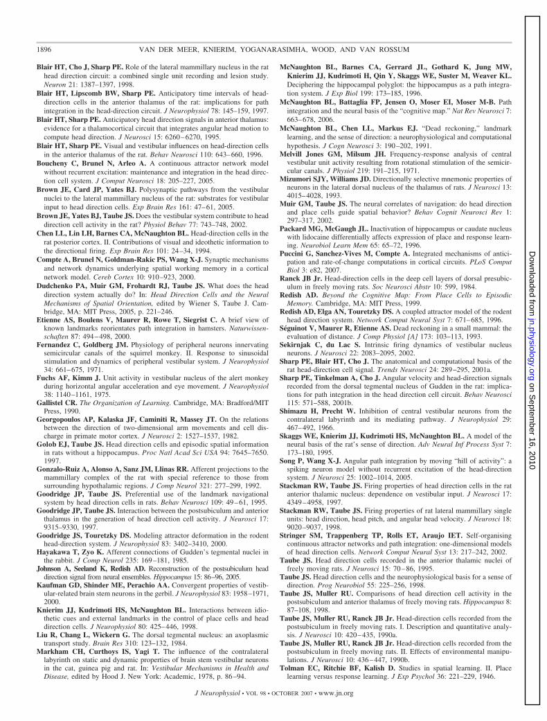
Blair HT, Cho J, Sharp PE. Role of the lateral mammillary nucleus in the rathead direction circuit: a combined single unit recording and lesion study.Neuron 21: 1387–1397, 1998.

Blair HT, Lipscomb BW, Sharp PE. Anticipatory time intervals of head-direction cells in the anterior thalamus of the rat: implications for pathintegration in the head-direction circuit. J Neurophysiol 78: 145–159, 1997.

Blair HT, Sharp PE. Anticipatory head direction signals in anterior thalamus:evidence for a thalamocortical circuit that integrates angular head motion tocompute head direction. J Neurosci 15: 6260–6270, 1995.

Blair HT, Sharp PE. Visual and vestibular influences on head-direction cellsin the anterior thalamus of the rat. Behav Neurosci 110: 643–660, 1996.

Boucheny C, Brunel N, Arleo A. A continuous attractor network modelwithout recurrent excitation: maintenance and integration in the head direc-tion cell system. J Comput Neurosci 18: 205–227, 2005.

Brown JE, Card JP, Yates BJ. Polysynaptic pathways from the vestibularnuclei to the lateral mammillary nucleus of the rat: substrates for vestibularinput to head direction cells. Exp Brain Res 161: 47–61, 2005.

Brown JE, Yates BJ, Taube JS. Does the vestibular system contribute to headdirection cell activity in the rat? Physiol Behav 77: 743–748, 2002.

Chen LL, Lin LH, Barnes CA, McNaughton BL. Head-direction cells in therat posterior cortex. II. Contributions of visual and ideothetic information tothe directional firing. Exp Brain Res 101: 24–34, 1994.

Compte A, Brunel N, Goldman-Rakic PS, Wang X-J. Synaptic mechanismsand network dynamics underlying spatial working memory in a corticalnetwork model. Cereb Cortex 10: 910–923, 2000.

Dudchenko PA, Muir GM, Frohardt RJ, Taube JS. What does the headdirection system actually do? In: Head Direction Cells and the NeuralMechanisms of Spatial Orientation, edited by Wiener S, Taube J. Cam-bridge, MA: MIT Press, 2005, p. 221–246.

Etienne AS, Boulens V, Maurer R, Rowe T, Siegrist C. A brief view ofknown landmarks reorientates path integration in hamsters. Naturwissen-schaften 87: 494–498, 2000.

Fernandez C, Goldberg JM. Physiology of peripheral neurons innervatingsemicircular canals of the squirrel monkey. II. Response to sinusoidalstimulation and dynamics of peripheral vestibular system. J Neurophysiol34: 661–675, 1971.

Fuchs AF, Kimm J. Unit activity in vestibular nucleus of the alert monkeyduring horizontal angular acceleration and eye movement. J Neurophysiol38: 1140–1161, 1975.

Gallistel CR. The Organization of Learning. Cambridge, MA: Bradford/MITPress, 1990.

Georgopoulos AP, Kalaska JF, Caminiti R, Massey JT. On the relationsbetween the direction of two-dimensional arm movements and cell dis-charge in primate motor cortex. J Neurosci 2: 1527–1537, 1982.

Golob EJ, Taube JS. Head direction cells and episodic spatial informationin rats without a hippocampus. Proc Natl Acad Sci USA 94: 7645–7650.1997.

Gonzalo-Ruiz A, Alonso A, Sanz JM, Llinas RR. Afferent projections to themammillary complex of the rat with special reference to those fromsurrounding hypothalamic regions. J Comp Neurol 321: 277–299, 1992.

Goodridge JP, Taube JS. Preferential use of the landmark navigationalsystem by head direction cells in rats. Behav Neurosci 109: 49–61, 1995.

Goodridge JP, Taube JS. Interaction between the postsubiculum and anteriorthalamus in the generation of head direction cell activity. J Neurosci 17:9315–9330, 1997.

Goodridge JS, Touretzky DS. Modeling attractor deformation in the rodenthead-direction system. J Neurophysiol 83: 3402–3410, 2000.

Hayakawa T, Zyo K. Afferent connections of Gudden’s tegmental nuclei inthe rabbit. J Comp Neurol 235: 169–181, 1985.

Johnson A, Seeland K, Redish AD. Reconstruction of the postsubiculum headdirection signal from neural ensembles. Hippocampus 15: 86–96, 2005.

Kaufman GD, Shinder ME, Perachio AA. Convergent properties of vestib-ular-related brain stem neurons in the gerbil. J Neurophysiol 83: 1958–1971,2000.

Knierim JJ, Kudrimoti HS, McNaughton BL. Interactions between idio-thetic cues and external landmarks in the control of place cells and headdirection cells. J Neurophysiol 80: 425–446, 1998.

Liu R, Chang L, Wickern G. The dorsal tegmental nucleus: an axoplasmictransport study. Brain Res 310: 123–132, 1984.

Markham CH, Curthoys IS, Yagi T. The influence of the contralaterallabyrinth on static and dynamic properties of brain stem vestibular neuronsin the cat, guinea pig and rat. In: Vestibular Mechanisms in Health andDisease, edited by Hood J. New York: Academic, 1978, p. 86–94.

McNaughton BL, Barnes CA, Gerrard JL, Gothard K, Jung MW,Knierim JJ, Kudrimoti H, Qin Y, Skaggs WE, Suster M, Weaver KL.Deciphering the hippocampal polyglot: the hippocampus as a path integra-tion system. J Exp Biol 199: 173–185, 1996.

McNaughton BL, Battaglia FP, Jensen O, Moser EI, Moser M-B. Pathintegration and the neural basis of the “cognitive map.” Nat Rev Neurosci 7:663–678, 2006.

McNaughton BL, Chen LL, Markus EJ. “Dead reckoning,” landmarklearning, and the sense of direction: a neurophysiological and computationalhypothesis. J Cogn Neurosci 3: 190–202, 1991.

Melvill Jones GM, Milsum JH. Frequency-response analysis of centralvestibular unit activity resulting from rotational stimulation of the semicir-cular canals. J Physiol 219: 191–215, 1971.

Mizumori SJY, Williams JD. Directionally selective mnemonic properties ofneurons in the lateral dorsal nucleus of the thalamus of rats. J Neurosci 13:4015–4028, 1993.

Muir GM, Taube JS. The neural correlates of navigation: do head directionand place cells guide spatial behavior? Behav Cognit Neurosci Rev 1:297–317, 2002.

Packard MG, McGaugh JL. Inactivation of hippocampus or caudate nucleuswith lidocaine differentially affects expression of place and response learn-ing. Neurobiol Learn Mem 65: 65–72, 1996.

Puccini G, Sanchez-Vives M, Compte A. Integrated mechanisms of antici-pation and rate-of-change computations in cortical circuits. PLoS ComputBiol 3: e82, 2007.

Ranck JB Jr. Head-direction cells in the deep cell layers of dorsal presubic-ulum in freely moving rats. Soc Neurosci Abstr 10: 599, 1984.

Redish AD. Beyond the Cognitive Map: From Place Cells to EpisodicMemory. Cambridge, MA: MIT Press, 1999.

Redish AD, Elga AN, Touretzky DS. A coupled attractor model of the rodenthead direction system. Network Comput Neural Syst 7: 671–685, 1996.

Seguinot V, Maurer R, Etienne AS. Dead reckoning in a small mammal: theevaluation of distance. J Comp Physiol [A] 173: 103–113, 1993.

Sekirnjak C, du Lac S. Intrinsic firing dynamics of vestibular nucleusneurons. J Neurosci 22: 2083–2095, 2002.

Sharp PE, Blair HT, Cho J. The anatomical and computational basis of therat head-direction cell signal. Trends Neurosci 24: 289–295, 2001a.

Sharp PE, Tinkelman A, Cho J. Angular velocity and head-direction signalsrecorded from the dorsal tegmental nucleus of Gudden in the rat: implica-tions for path integration in the head direction cell circuit. Behav Neurosci115: 571–588, 2001b.

Shimazu H, Precht W. Inhibition of central vestibular neurons from thecontralateral labyrinth and its mediating pathway. J Neurophysiol 29:467–492, 1966.

Skaggs WE, Knierim JJ, Kudrimoti HS, McNaughton BL. A model of theneural basis of the rat’s sense of direction. Adv Neural Inf Process Syst 7:173–180, 1995.

Song P, Wang X-J. Angular path integration by moving “hill of activity”: aspiking neuron model without recurrent excitation of the head-directionsystem. J Neurosci 25: 1002–1014, 2005.

Stackman RW, Taube JS. Firing properties of head direction cells in the ratanterior thalamic nucleus: dependence on vestibular input. J Neurosci 17:4349–4958, 1997.

Stackman RW, Taube JS. Firing properties of rat lateral mammillary singleunits: head direction, head pitch, and angular head velocity. J Neurosci 18:9020–9037, 1998.

Stringer SM, Trappenberg TP, Rolls ET, Araujo IET. Self-organisingcontinuous attractor networks and path integration: one-dimensional modelsof head direction cells. Network Comput Neural Syst 13: 217–242, 2002.

Taube JS. Head direction cells recorded in the anterior thalamic nuclei offreely moving rats. J Neurosci 15: 70–86, 1995.

Taube JS. Head direction cells and the neurophysiological basis for a sense ofdirection. Prog Neurobiol 55: 225–256, 1998.

Taube JS, Muller RU. Comparisons of head direction cell activity in thepostsubiculum and anterior thalamus of freely moving rats. Hippocampus 8:87–108, 1998.

Taube JS, Muller RU, Ranck JB Jr. Head-direction cells recorded from thepostsubiculum in freely moving rats. I. Description and quantitative analy-sis. J Neurosci 10: 420–435, 1990a.

Taube JS, Muller RU, Ranck JB Jr. Head-direction cells recorded from thepostsubiculum in freely moving rats. II. Effects of environmental manipu-lations. J Neurosci 10: 436–447, 1990b.

Tolman EC, Ritchie BF, Kalish D. Studies in spatial learning. II. Placelearning versus response learning. J Exp Psychol 36: 221–229, 1946.

1896 VAN DER MEER, KNIERIM, YOGANARASIMHA, WOOD, AND VAN ROSSUM

J Neurophysiol • VOL 98 • OCTOBER 2007 • www.jn.org

on Septem

ber 16, 2010 jn.physiology.org

Dow

nloaded from

Trappenberg TP. Fundamentals of Computational Neuroscience. Oxford,UK: Oxford Univ. Press, 2002.

Vidal P-P, Sans A. Vestibular system. In: The Rat Nervous System (3rd ed.),edited by Paxinos G. New York: Academic, 2004, p. 965–996.

Wiener SI, Arleo A, Dejean C, Boucheny C, Khamassi M, Zugaro MB.Optic field flow signals update the activity of head direction cells in the ratanterodorsal thalamus. Soc Neurosci Abstr 209.2, 2004.

Wiener SI, Taube JS. Head Direction Cells and the Neural Mechanisms ofSpatial Orientation. Cambridge, MA: MIT Press, 2005.

Xie W, Hahnloser RHR, Seung HS. Double ring model of the head-directionsystem. Phys Rev E 66: 41902–41910, 2002.

Yoganarasimha D, Yu X, Knierim JJ. Head direction cell representationsmaintain internal coherence during conflicting proximal and distal cue

rotations: comparison with hippocampal place cells. J Neurosci 26: 622–631, 2006.

Yu X, Yoganarasimha D, Knierim JJ. Backward shift of head directiontuning curves of the anterior thalamus: comparison with ca1 place fields.Neuron 52: 717–729, 2006.

Zhang K. Representation of spatial orientation by the intrinsic dynamics of thehead-direction cell ensemble: a theory. J Neurosci 16: 2112–2126, 1996.

Zugaro MB, Arleo A, Berthoz A, Wiener SI. Rapid spatial reorientation andhead direction cells. J Neurosci 23: 3478–3482, 2003.

Zugaro MB, Tabuchi E, Fouquier C, Berthoz A, Wiener SI. Activelocomotion increases peak firing rates of anterodorsal thalamic head direc-tion cells. J Neurophysiol 86: 692–702, 2001.

1897HD ANTICIPATION MODEL

J Neurophysiol • VOL 98 • OCTOBER 2007 • www.jn.org

on Septem

ber 16, 2010 jn.physiology.org

Dow

nloaded from