Max flows in O(nm) time, or better

James B. Orlin∗

Revised: July 25, 2012

Abstract

In this paper, we present improved polynomial time algorithms for the max flow problemdefined on a network with n nodes and m arcs. We show how to solve the max flow problem inO(nm) time, improving upon the best previous algorithm due to King, Rao, and Tarjan, whosolved the max flow problem in O(nm logm/(n log n) n) time. In the case that m = O(n), weimprove the running time to O(n2/ log n).

We further improve the running time in the case that U∗ = Umax/Umin is not too large,where Umax denotes the largest finite capacity and Umin denotes the smallest non-zero capacity.If log(U∗) = O(n1/3 log−3 n), we show how to solve the max flow problem in O(nm/ log n) steps.In the case that log(U∗) = O(logk n) for some fixed positive integer k, we show how to solve themax flow problem in O(n8/3) time. This latter algorithm relies on a subroutine for fast matrixmultiplication.

1 Introduction

Network flow problems form an important class of optimization problems and are central problemsin operations research, computer science and combinatorial optimization. A special network flowproblem, the max flow problem, has been widely investigated since the seminal research of Fordand Fulkerson in the 1950s. The max flow problem has applications in transportation, logistics,telecommunications, and scheduling. Numerous efficient algorithms for this problem exist including[7] and [4]. A comprehensive discussion of such algorithms and applications can be found in [1].

We consider the max flow problem on a directed graph with n nodes, m arcs, and integervalued arc capacities (possibly infinite), in which the largest finite capacity is bounded by U .The fastest strongly polynomial time algorithm is due to King et al. [21]. Its running time isO(nm logm/(n logn) n). When m = Ω(n1+ε) for any positive constant ε, the running time is O(nm).When m = O(n log n), the running time is O(nm log n). The fastest weakly polynomial timealgorithm is due to Goldberg and Rao [16]. Their algorithm solves the max flow problem as asequence of O(logU) scaling phases, each of which transforms a ∆-optimal flow into a ∆/2-optimalflow. The running time per scaling phase is O(Λm log(n2/m)), where Λ = minn2/3,m1/2.

Our contribution. We show that the max flow problem can be solved in O(nm+m31/16 log2 n)time. When m = O(n(16/15)−ε), this running time is O(nm). Because the algorithm by King etal. [21] solves the max flow problem in O(nm) time for m > n1+ε , our improvement establishesthat the max flow problem can be solved in O(nm) time for all n and m.∗Sloan School of Management and Operations Research Center, Massachusetts Institute of Technology, Cambridge,

Massachusetts 02139, E-mail: jorlin@mit.edu

1

We also develop an O(n2/ log n) algorithm for max flow problems in which m = O(n).Our algorithm solves the max flow problem as a sequence of improvement phases, similar to the

scaling phases in the Goldberg-Rao algorithm. We obtain a strongly polynomial time algorithmby replacing the residual network of the ∆-improvement phase by a more compact representation.The bottleneck operation for our algorithms is the creation of the compact representation. Theother bottleneck operation is the transformation of flows in the compact network to flows in theresidual network.

In addition, we present improved polynomial time algorithms for the max flow problem underseveral different parameter settings. Let U∗ = (Umax/Umin), where Umax is the largest finite capac-ity, and Umin is the smallest non-zero capacity. If U∗ is not too large (e.g., logU∗ = O(n1/3/ log3 n)),then one can solve the max flow problem in strongly polynomial time by first using the Goldberg-Rao algorithm to obtain a ∆-optimal flow for ∆ = Umin/2, and subsequently using our stronglypolynomial time algorithm to transform the ∆-optimal flow into an optimal flow. Suppose that welet T (n,m) denote the running time to find an optimal flow starting with the ∆-optimal flow. Weshow that

1. T (n,m) = O(nm/ log n) for all n and m.

2. T (n,m) = O(n17/12m5/8 + n1+2ω/3) = O(n8/3).

Our algorithm relies on fast matrix multiplication, which runs in O(nω) time, where ω is 2.3727.This bound is due to Williams [24], which improves upon the previous bound due to Coppersmithand Winograd [8]. The time to find the ∆-optimal flow is O(n2/3m). The time it takes to find anoptimal flow is O(n8/3). (The O bounds ignore factors that are polynomial in log n.) In the casethat m = Ω(n2), this bound is a factor n1/3 faster than the best previous strongly polynomial timemax flow algorithm.

Our paper is organized as follows. In Section 2, we provide preliminary notation and definitions.In Section 3, we describe how the max flow problem is solved as a sequence of improvement phases.In Section 4, we describe the abundance graph and how contraction can speed up the algorithm.In Section 5, we show how abundant directed cycles as well as some other arcs may be contractedso as to result in a smaller max flow problem. In Section 6, we explain how nodes incident toonly abundant arcs may be “compacted”. Compaction is a concept that is new to this paper. InSection 7, we show how to run the improvement phase for the max flow problem on the compactnetwork (when appropriate) rather than on the original network. We reduce the total running timeto O(nm + m31/16 log2 n), which is O(nm) time if m = O(n(16/15)−ε). The bottleneck operationfor our algorithm is the time it takes to maintain the transitive closure of the “abundance graph”.In Section 8, we show how to solve the max flow problem in O(n2/ log n) time in the case thatm = O(n). In Section 9, we show how to speed up the algorithm further if logU∗ is not too large.

2 Preliminary notation, definitions, and lemmas

We consider a directed graph G = (N,A) with node set N and arc set A. We let n = |N | and welet m = |A|. Each arc (i, j) ∈ A has an associated integral capacity uij . We permit some of thearc capacities to be infinite. We let Umax denote the maximum of the finite arc capacities. We letUmin denote the minimum of the non-zero arc capacities.

There are two distinguished nodes in N : a source s and a sink t. A single commodity must berouted through G from s to t. The arcs incident to s or t are referred to as external arcs. The

2

remaining arcs are called internal arcs. A node i is internal if i 6= s and i 6= t. To simplify notation,we assume without loss of generality that whenever an internal arc (i, j) is in A, arc (j, i) is also inA. For every internal node i, we assume that (s, i) and (i, t) are in A, possibly with a capacity of0.

To contract an arc (i, j) is to replace the nodes i and j by a single new node, referred to as thecontracted node. Any arc that was formerly incident to node i or j before contraction is incidentto the contracted node subsequently. Contraction is a standard operation in graph and networkalgorithms.

A flow is a function x : A→ R+ ∪ 0 that satisfies the flow conservation constraints; that is,∑j:(i,j)∈A

xij −∑

j:(j,i)∈A

xji = 0 for all i ∈ N \ s, t.

A flow x is called feasible if it obeys the capacity constraints, that is, xij ≤ uij for each arc(i, j) ∈ A. We refer to xij as the flow on arc (i, j). The value of a flow x is the net flow out ofthe source, which is equal to the net flow into the sink. In a max flow problem, one seeks a feasibleflow whose value is maximum.

Suppose that x is a feasible flow. For each internal node i, the residual capacity of arc (s, i) isrsi = usi − xsi. The residual capacity of arc (i, t) is rit = uit − xit. For each internal arc (i, j) ∈ A,rij = uij + xji − xij . The residual capacity expresses how much additional flow can be sent from ito j, starting with the flow x. We let r[x] denote the vector of residual capacities. Often, we willdenote the residual capacities more briefly as r. The residual network is denoted G[r]. The arcs(i, s) and (t, i) are not present in G and they also not present in G[r].

An s-t cut is a partition of the node set N into two parts, S and T , such that s ∈ S and t ∈ T .The capacity of the cut (S, T ) is u(S, T ) =

∑i∈S,j∈T uij . If r is the vector of residual capacities and

if (S, T ) is an s-t cut, then the residual capacity of the cut (S, T ) is r(S, T ) =∑

i∈S,j∈T rij . Thefollowing is the max-flow min-cut theorem of Ford and Fulkerson [11], as applied to the residualnetwork.

Lemma 1. (Max residual flow, min residual cut). Suppose that r is a vector of residualcapacities and (S, T ) is an s-t cut. Then r(S, T ) is an upper bound on the maximum amount offlow that can be sent from source to sink in the residual network G[r]. Moreover, the maximumflow with respect to r is the minimum residual capacity of an s-t cut.

We let A(j) denote the subset of arcs incident to node j. We say that A′(j) is an anti-symmetricsubset of A(j) if for every arc (i, j) ∈ A(j), either (i, j) ∈ A′(j) or (j, i) ∈ A′(j) but not both. Notethat if A′(j) is antisymmetric, then (s, j) ∈ A′(j) and (j, t) ∈ A′(j).

Lemma 2. (Anti-symmetry lemma). Suppose that A′(j) is an anti-symmetric subset of A(j).Suppose further that x is a feasible flow, and r = r[x]. Then

∑(i,j)∈A′(j)

rij −∑

(j,i)∈A′(j)

rji =∑

(i,j)∈A′(j)

uij −∑

(j,i)∈A′(j)

uji.

Proof. We note that rij = uij − xij + xji. The lemma is true because of the following.

3

∑(i,j)∈A′(j)

(uij − rij)−∑

(j,i)∈A′(j)

(uji − rji)

=∑

(i,j)∈A′(j)

(xji − xij) +∑

(j,i)∈A′(j)

(xji − xij) =∑

(i,j)∈A(j)

(xji − xij) = 0.

Suppose that P is a directed path in G from node i to node j, and suppose that (i, j) ∈ A.Suppose further that |P | ≥ 2. To transfer δ units of capacity from path P to arc (i, j) is to reduceuk` by δ of each arc (k, `) of P and to increase uij by δ.

Lemma 3. (Capacity transfer lemma). Let P be a path in G from node i to node j. Let (S, T )be an s-t cut. Suppose that u′ is obtained from u by transferring δ units of capacity from P to arc(i, j). Then u′(S, T ) ≤ u(S, T ).

Proof. Except in the case that i ∈ S and j ∈ T , the lemma is trivially true because u′k` ≤ uk` unlessi = k and j = `. Suppose now that i ∈ S and j ∈ T . Let ` be the first node of P that is in T , andlet k be the preceding node of P . Then u(S, T )− u′(S, T ) ≤ uk` − u′k` + uij − u′ij = δ − δ = 0.

In general, transferring capacity from paths to arcs decreases the amount of flow that can besent from source to sink. In essence it requires that δ units of the capacity of each of the arcs inP be reserved for sending flow from i to j. In Section 6, we will see an important special case oftransferring capacity from a path to an arc that does not result in a decrease in the max flow.

3 Improvement phases

Our algorithm solves the max flow problem as a sequence of improvement phases. The input for animprovement phase is a flow x, a vector r = r[x] of residual capacities, and an s-t cut (S, T ). Wetypically denote the input for an improvement phase as the triple (r, S, T ). We refer to the phaseas the ∆-improvement phase, where ∆ = r(S, T ).

The output of the ∆-improvement phase is a flow x′, a vector r′ = r[x′] of residual capacitiesand an s-t cut (S′, T ′) such that r′(S′, T ′) ≤ ∆/(4m).

We will run the improvement phase either on the network G or on a “compact network” Gc,described later.

4 ∆-abundant arcs and the abundance graph

Let (r, S, T ) be the input for an improvement phase, and let ∆ = r(S, T ). An arc (i, j) is called∆-abundant if rij ≥ 2∆. We sometimes refer to it as abundant if ∆ is obvious from context. Thechange in flow in any arc is at most ∆ during an improvement phase. Therefore, the followinglemma is true.

Lemma 4. Suppose that (r, S, T ) is the input at the beginning of the ∆-improvement phase, where∆ = r(S, T ). If arc (i, j) is ∆-abundant at the beginning of the ∆-improvement phase, then (i, j)remains abundant at all subsequent improvement phases.

4

Abundant arcs play two roles in the speed-up of our max flow algorithm. (1) Directed cycles ofabundant arcs are “contracted” into a single node. The contracted arcs are expanded subsequent tothe algorithm identifying an optimal flow in the contracted graph. (2) A node can be “compacted”if every incident arc is either abundant or it has very small capacity. Compacted nodes are notpresent in the compact network. We describe compaction in Section 6.

The abundance graph is the graph with node set N and whose arc set is the set of abundantarcs. We denote it as Gab. By Lemma 4, once an arc becomes abundant, it remains abundant. Theabundance graph increases dynamically over time.

An arc (i, j) is in the transitive closure of Gab if there is a directed path in Gab from node ito node j. Our algorithm maintains the transitive closure of Gab over all iterations. This maybe accomplished in O(nm) time using Italiano’s [18] algorithm for dynamically maintaining thetransitive closure of a graph.

If there is an abundant path from node i to node j, we denote it as i⇒ j. The transitive closurealgorithm maintains a path from node i to node j whenever i⇒ j. If there is more than one path,it will maintain the first path it determines. It maintains paths implicitly by using a matrix M. Ifthere is a path from node i to node j in Gab, then Mij is the node that precedes j on the path inGab from i to j. The time it takes to reconstruct a path P from the matrix M is O(|P |).

The transitive closure algorithm is valid even if Gab contains directed cycles. However, as we willsee in Section 5, our algorithm contracts any abundant directed cycles. Contraction of abundantcycles does not increase the time needed to maintain the dynamic transitive closure.

5 Contraction of abundant cycles

If the abundance graph contains the internal arcs (i, j) and (j, i), then we can contract nodes i andj into a single node, and find an optimal flow in the contracted graph. After obtaining an optimalflow in this contracted graph, one can then expand the contracted node into their original pair ofarcs (i, j) and (j, i). The flow in the expanded graph can be made feasible by sending flow on (i, j)or (j, i), whichever is needed in order to balance the flow in nodes i and j.

We illustrate this contraction on arcs (5, 6) and (6, 5) in Figures 1 and 2. After contraction,the total change in flow in each arc is less than 2∆. When the node labeled 5-6 is ultimatelyexpanded, it is possible that the flow conservation constraints are violated for nodes 5 and 6, butby an amount that is less than 2∆. By sending flow from 5 to 6 or from 6 to 5, the conservationof flow constraints are reestablished.

It is also possible to contract abundant external arcs. We illustrate this type of contractionon arcs (s, 1) and (3, t) in Figures 3 and 4. When the nodes labeled s-1 and 3-t are ultimatelyexpanded, it is possible that the flow conservation constraints are not satisfied at nodes 1 or 3.Flow conservation can be reestablished by sending flow in (s, 1) and (3, t).

In addition, one can contract any abundant cycle of internal arcs.

The total time for contraction in an improvement phase is O(m). The time for expansionof contracted cycles is also O(m). For more details on contraction and expansion of cycles, seeGoldberg and Rao [16].

5

1 2

3 4

5 6

≥ 2 Δ

≥ 2 Δ

Figure 1. A residual network in which arcs (5, 6) and (6, 5) are both abundant.

1 2

3 4

5 5-­‐6

Figure 2. The residual network aCer contracDng the arcs (5, 6) and (6, 5).

1 2

3 4

t s

≥ 2 Δ

≥ 2 Δ

1

2

3

4

3-­‐t s-­‐1

1 2

3 4

6 5

≥ 2 Δ ≥ 2 Δ

≥ 2 Δ

≥ 2 Δ

≥ 2 Δ

1 2

3 4

Figure 3. A residual network in which arcs (s, 1) and (3, t) are both abundant.

Figure 4. The residual network aCer contracDng (s, 1) and (3, t).

Figure 5. Part of a network in which nodes 5 and 6 are both strongly compacDble. The solid arcs are all abundant.

Figure 6. The subgraph of the strongly compact network obtained from Figure 5.

6

6 The compact network

In this section, we will define compact networks. We start by showing how to construct an inter-mediate version of the compact network that we refer to as the “strongly compact network”. Thisnetwork is essentially the same as the residual network except that we will eliminate any node forwhich all incident arcs are abundant. Subsequently, we will define the compact network and showhow to construct it.

Algorithm 1. A procedure for creating the strongly compact network Gsc = (N sc, Asc).

Step 1. Iteratively contract abundant cycles. Iteratively contract abundant external arcs. Let(r, S, T ) denote the input after contraction of the abundant cycles.

Step 2. Let N sc be the subset of nodes incident to a non-abundant arc whose residual capacity ispositive. A node in N\N sc is referred to as strongly compactible.

Step 3. Asc = A1 ∪ A2, where A1 = (i, j) ∈ A : i ∈ N sc and j ∈ N sc, and A2 = (i, j) : i ∈N sc and j ∈ N sc and i⇒ j. An (i, j) ∈ A1 is referred to as an original arc and its capacityis rij . An arc (i, j) ∈ A2 is referred to as a pseudo-arc and its residual capacity is 2∆.

Algorithm 1 runs in O(m+ |Asc|) time. We can create each pseudo-arc in O(1) time because weare maintaining the transitive closure of the abundance graph. (We will only create the compactnetworks in cases in which |Asc| = O(m9/8), a bound that arises from the analysis.)

We illustrate this construction in Figures 5 and 6. In Figure 6, nodes 5 and 6 do not appearbecause neither node was incident to a non-abundant arc with residual capacity. Figure 6 includespseudo-arcs from nodes 1 and 4 to nodes 2 and 3.

Theorem 1. Let v∗ be the max flow in the residual network G[r], and let vsc be the max flow inthe strongly compact network Gsc. Then vsc = v∗.

Proof. Consider first a flow in Gsc. This can be transformed into a flow in G[r] by replacing theflows in pseudo-arcs of Gsc by flows on the corresponding paths in G[r].

Now consider a flow x in G[r]. One can use flow decomposition (see, e.g., Ahuja et al. [1]) torepresent x as the sum of flows on paths from s to t. For each path P in the flow decomposition,we carry out the following additional operations. Subdivide P into the union of subpaths, whereeach subpath begins and ends at a node in N sc, but the other nodes of the subpath are in N\N sc.If P ′ is a subpath of P from node i to node j, then replace the flow on the subpath P ′ by flow inthe corresponding pseudo-arc (i, j) ∈ Asc. Repeating this process yields a flow decomposition inGsc, which, in turn, can be expressed as a flow in Gsc.

We next describe how to obtain the ∆-compact network, which is similar to the strongly com-pact network, but which may contain far fewer nodes. Our O(nm) algorithm for the max flowproblem exploits the fact that the running time to find an approximate max flow in the ∆-compactnetwork may be less than the time it takes to find the approximate max flow in the original network.

An arc (i, j) is said to have small capacity with respect to ∆ if rij + rji < ∆/(64m2). An arc(i, j) is said to have medium capacity with respect to ∆ if rij ≥ ∆/(64m2) and if rij + rji < 4∆.

An internal arc (i, j) is referred to as anti-abundant if rij < 2∆ and rji ≥ 2∆. An external arc(s, j) or (j, t) is referred to as anti-abundant if it is not abundant.

7

The arcs of the ∆-compact network will consist of original arcs and pseudo-arcs. The abun-dant pseudo-arcs will be created in the same manner as in Algorithm 1. There will also be non-abundant pseudo-arcs that will be created by transferring capacity from a path P of anti-abundantarcs. (Transferring capacity was described in Section 2.) After transferring flows on paths, ourconstruction of the compact network is very similar to our construction of the strongly compactnetwork.

Our analysis relies on a potential function. For a given node j ∈ N , vector r of residualcapacities and for a subset A of arcs, we define the potential function Φ(j, r, A) as follows.

Φ(j, r, A) =∑

(i,j)∈ eArij −

∑(j,i)∈ eA

rji. (1)

Let A′(∆) denote the set of anti-abundant arcs at the ∆-improvement phase. In the next lemma,the potential function is defined on A = A′. We rely on other choices of A in the proof of Lemma2.

Lemma 5. Let (S, T ) be an s-t cut in G with r(S, T ) ≤ ∆, and let A′ = A′(∆). Suppose thatP ⊆ A′ is a path from node i to node j, and suppose that (i, j) ∈ A′. Let r′ be obtained from r bytransferring δ units of residual capacity from path P to arc (i, j). Then (1) Φ(k, r′, A′) = Φ(k, r, A′)for each k ∈ N , and (2) r′(S, T ) = r(S, T ).

Proof. The proof of statement (1) is straightforward. We now consider statement (2). Statement(2) is trivially true if |P | = 1. Assume that |P | ≥ 2, and let P = i1, i2, . . . , ik. The lemma is clearlytrue in the case that every node of P is in S or if every node of P is in T . So, we consider thecase in which at least one node of P is in S and at least one node of P is in T . Since the reversalof each arc of (P ) is abundant, and since r(S, T ) ≤ ∆, there must be an index ` ∈ [1, k − 1] suchthat (a) ij ∈ S for j ≤ `, and (b) ij ∈ T for j > `. Under these circumstances, one can verify thatr′(S, T ) = r(S, T ).

We say that a node j is ∆-compactible if |Φ(j, r′, A′)| < ∆/(16nm) and if j is not incident to amedium capacity arc. We say that node j is very ∆-compactible if it is ∆-compactible and if everyincident anti-abundant arc has capacity less than ∆/(16nm). The proof of the following lemma isimmediate from our definition of the potential function Φ.

Lemma 6. Suppose that node j is ∆-compactible. Suppose further that there is no pair of anti-abundant arcs (i, j) and (j, k) with positive residual capacity. Then j is very ∆-compactible.

Prior to constructing the compact network at the ∆-improvement phase, our algorithm williteratively transfer the residual capacity of a path to a pseudo-arc. (Step 3A of Algorithm 2).The transfer of capacities will not affect the maximum flow value. Each transfer of capacities willeliminate at least one anti-abundant arc from the network. The transfer of capacities will continueuntil every ∆-compactible node becomes very ∆-compactible.

We say that a path P has transferrable residual capacity if (i) |P | ≥ 2, (ii) r(P ) > 0, and (iii)each arc of P is anti-abundant. If P is a path from node i to node j such that P has transferrablecapacity, then to transfer the residual capacity of P is to transfer r(P ) units of capacity from Pto (i, j). If arc (i, j) were not in A, we would add (i, j) as an anti-abundant pseudo-arc prior totransferring the capacity.

We say that a node j is ∆-critical if it is not ∆-compactible. The set of nodes in the ∆-compactnetwork are the ∆-critical nodes. We next bound the total number of nodes in compact networks.

8

Theorem 2. The total number of ∆-critical nodes over all improvement phases is O(m).

Proof. Let ∆k denote the parameter for the k-th improvement phase. Our improvement algorithmensures that for each k, ∆k+1 ≤ ∆k/(4m).

We first consider nodes in compact networks that are incident to arcs of medium capacity. Letr denote the residual capacities after Step 1 of Algorithm 1 at Improvement Phase k. Let r′ denotethe residual capacities at the beginning of Phase k+ 4. If (i, j) or (j, i) is of medium capacity withrespect to ∆k, then ∆k/(64m2) ≤ rij + rji ≤ 4∆k. Then r′ij + r′ji = rij + rji > 4∆k+3. It followsthat each arc is of medium capacity for at most four improvement phases. And the total numberof medium arcs over all improvement phases is O(m).

We next consider the remaining ∆-critical nodes, which we refer to as ∆-special nodes. If nodej is ∆-special, then |Φ(j, r, A′)| ≥ ∆/(16nm) and there are no medium capacity arcs incident to j.

We claim the following: if node j is ∆-special, then within four more improvement phases, nodej will be on an abundant directed cycle, and will thus be contracted. If the claim is true, then wewill have shown that the number of ∆-special nodes over all improvement phases is O(n), which willcomplete the proof that the total number of ∆-critical nodes is O(m). (We assume that m ≥ n.)

Suppose that node j is ∆-special. Let A′(j) be the set of arcs arcs incident to node j that areanti-abundant at Phase k. Let A′′(j) consist of arc (s, j) plus all of the arcs directed out of nodej that are neither abundant nor anti-abundant at Phase k. (All of these arcs have small capacitywith respect to ∆k). Then A′(j)∪A′′(j) is an anti-symmetric subset of A(j). By Lemma 2 and byLemma 5, Φ(j, r, A′(j) ∪A′′(j)) = Φ(j, r′, A′(j) ∪A′′(j)). Therefore,

|Φ(j, r′, A′(j))| ≥ |Φ(j, r, A′(j))| − |Φ(j, r, A′′(j))| − |Φ(j, r′, A′′(j))| (2)

≥ ∆k/(16nm)− 2n∆k/(64m2) (3)≥ ∆k/(32nm) > 4n∆k+4. (4)

Inequality (3) relies on the fact that there at most n arcs in A′′(j), each with capacity less than∆k/(64m2). Since A′(j) has fewer than 2n arcs, inequality (4) implies that there must be an arca ∈ A′(j) such that r′a ≥ 2∆k+4. Since the reversal of arc a is also abundant, it follows that arc aand its reversal is an abundant cycle, and thus arc a would be contracted.

We next show how to create the ∆-compact network Gc = (N c, Ac). The node set N c is the setof ∆-critical nodes. To obtain the arc set Ac, one first transfers capacities on paths whose arcs areanti-abundant.

Algorithm 2. A procedure for creating the ∆-compact network Gc = (N c, Ac).

Step 1. Iteratively contract abundant cycles. Iteratively contract abundant external arcs.

Step 2. Let N c be the set of ∆-critical nodes.

Step 3A. If there is a ∆-compactible node with an entering anti-abundant arc and a leavinganti-abundant arc, find a path P with transferrable residual capacity such that the first andlast nodes of P are in N c and every other node of P is in N\N c. (Such a path will exist).Transfer the residual capacity from this path to a pseudo-arc. Continue finding paths withtransferrable residual capacity until there is no ∆-compactible node with an entering anti-abundant arc and a leaving anti-abundant arc. (In Section B, we will show how to implementStep 3A efficiently using dynamic trees.)

9

Step 3B. Let r′ denote the residual capacities of arcs and pseudo-arcs after Step 3A. Let Ac =A1 ∪A2, where A1 = (i, j) : i ∈ N c , j ∈ N c, and r′ij > 0, and A2 = (i, j) : i ∈ N c and j ∈N c and i⇒ j. An arc (i, j) ∈ A1 has capacity r′ij . An arc in A2 is referred to as a pseudo-arcand has residual capacity 2∆.

Theorem 3. Let v∗ be the max flow in the residual network G[r], and let v′ be the max flow in the∆-compact network Gc . Then v′ ≤ v∗ < v′ + ∆/8m.

Proof. Contracting abundant cycles or abundant external arcs does not affect the max flow value,nor does it increase the number of arcs.

We now consider Step 3A. Lemma 5 shows that transferring flow from transferrable paths topseudo-arcs does not affect the value of the max flow, nor does it affect the potential function Φ.

We now consider Step 3B. If the only arcs incident to the ∆-compactible nodes were abundantarcs, then by Theorem 1, the max flow in Gc would be the same as the max flow in G[r]. However,in creating Gc, we also eliminate all small capacity arcs incident to ∆-compactible nodes as wellas the anti-abundant arcs incident to the ∆-compactible nodes after the transfer of capacity frompaths. There are at most m arcs with small capacity, and the sum of their capacities is less thanm(∆/(64m2)) = ∆/(64m). The total capacity of anti-abundant arcs incident to ∆-compactiblenodes after Step 3A is less than n∆/(16nm) = ∆/(16m). We conclude that v′ ≤ v∗ ≤ v′ +∆/(64m) + ∆/(16m) < v′ + ∆/(8m).

Theorem 3 establishes that the transformation used to create the ∆-compact network decreasesthe maximum amount of flow by at most ∆/(8m).

7 Maximum flows in O(nm) time

In this section, we show that the running time for our max flow algorithm is O(nm), and thebottleneck is due to the maintenance of the transitive closure of Gab.

The procedure improve-approx-2 finds an approximately optimal flow in an improvement phaseby considering three different cases. Let c denote the number of ∆-critical nodes. (i) If c > m9/16,then the procedure finds a ∆′-optimal solution on G[r], where ∆′ = ∆/(4m). (ii) If m1/3 ≤c < m9/16, then the procedure finds a ∆′/2-optimal solution on Gc, and transforms this into a ∆′-optimal solution on G[r]. If c < m1/3, then the procedure first chooses a parameter Γ, where Γ < ∆′.It then determines an optimal flow on what is referred to as the “(∆,Γ)-compact network”, andtransforms this flow into a Γ-optimal flow for G. We will show that this third case occurs O(m2/3)times, and the running time for the flow subroutines on each of these instances is O(m).

The (∆,Γ)-compact network is created in the same way as the ∆-compact network with thefollowing exception. For a node j to be (∆,Γ)-critical, it is incident to an arc (i, j) such that(i) Γ/(64m2) < rij + rji < 4∆ or (ii) |Φ(j, r, A′)| ≥ Γ/(16nm). As before, abundance and anti-abundance are still defined with respect to ∆.

The following procedure transforms a ∆-optimal solution into a ∆/(4m)-optimal solution.

Procedure improve-approx-2(r, S, T );01. ∆ := r(S, T )02. let c be the number of ∆-critical nodes03. if c > m9/16 then find a ∆/(4m)-optimal flow on the residual network G[r]04. else, if m1/3 ≤ c < m9/16 then05. let G′ denote ∆-compact network

10

06. find a ∆/(8m)-optimal flow x′ on G′

07. transform the flow x′ into a ∆/(4m)-optimal flow x∗ on G[r]08. else, if c < m1/3 then09. choose the minimum value Γ such that the number of nodes10. in the (∆,Γ′)-compact network is less than 2m1/3

11. let G′ denote (∆,Γ)-compact network12. find an optimal flow x′ on G′

13. transform the flow x′ into a Γ-optimal flow x∗ on G[r]

In the following lemma, when we refer to the time to find flows in improve-approx-2, we arereferring steps 3 and 6. We are not referring to the time to create the compact networks.

Lemma 7. Let c be the number of ∆-critical nodes for the procedure improve-approx-2. If c ≥ m1/3,then the running time of the flow subroutine is O(cm15/16 log2 n).

Proof. If c > m9/16, then the running time per improvement phase is O(m3/2 log2 n). Multiplyingthe running time by c/m9/16 shows that the running time is O(cm15/16 log2 n). If m1/3 < c <m9/16, then the running time for determining an approximate max flow on the compact network isO(c8/3 log n), which is O(cm15/16 log n).

Lemma 8. Let c be the number of ∆-critical nodes for the procedure improve-approx-2. The numberof phases for which c < m1/3 is O(m2/3). The running time of the flow subroutines that find theoptimal flow in the compact network is O(m) for each of these phases.

Proof. The final statement of the theorem is obvious. If the number of nodes is c and if c < m1/3,then the running time per max flow is O(c3) = O(m).

We next prove that the number of improvement phases is O(m2/3). We first note that thecondition for a node to be (∆,Γ)-critical is more restrictive than the condition that a node be∆-critical. Therefore, by Theorem 2, the number of nodes in compact (∆,Γ)-compact networks isO(m) over all improvement phases.

Suppose that in the k-th improvement phase, the parameters are ∆k and Γk and that thereare additional improvement phases beyond Phase k. By our rule for choosing Γk, the number of(∆k,Γk/2)-critical nodes is greater than 2m1/3. Using a similar argument to the one in the proofof Theorem 2, we will show that within four more scaling phases m1/3 arcs of medium capacity willhave large capacity, or m1/3 nodes will be contracted or both. This will establish that there areO(m2/3) such phases.

We have already established that ∆k+1 ≤ Γk. Any arc that is medium capacity with respectto Γk/2 will become abundant or anti-abundant within 4 additional improvement phases. Supposethat node j is (∆k,Γk/2)-critical but is not incident to an arc that is medium capacity with respectto Γk/2. Then node k will be contracted within four more improvement phases. This shows thatthe number of phases for which c < m1/3 is O(m2/3).

Theorem 4. For m = O(n16/15−ε), the max flow problem is solvable in O(nm) time by iterativelycalling the procedure improve-approx-2.

Proof. We first consider the time spent in flow operations; i.e., Steps 4, 7, and 13 of procedureimprove-approx-2. The total number of ∆-critical nodes over all improvement phases is O(m). ByLemma 7, the time to find the approximate max flows is O(m31/16 log2 n) over all phases with atleast m1/3 ∆-critical nodes. By Lemma 8, the number of improvement phases is O(m2/3). If there

11

are fewer than m1/3 ∆-critical nodes, the time for the flow operations is O(m). Thus, the totaltime for finding flows in these improvement phases is bounded by O(m5/3).

The remaining operations to consider are the following: (1) the time to contract abundant cyclesand to expand them; (2) the time to create the abundant pseudo-arcs of the compact networks;(3) the time to transform flows in abundant pseudo-arcs of the compact networks into flows onpaths in the original network; (4) the time to transfer capacities from paths of anti-abundant arcsto pseudo-arcs of the compact networks, and (5) the time to transform flows in the non-abundantpseudo-arcs of the compact networks into flows on paths in the original network.

We have already stated that the time to contract abundant cycles and expand them is O(m)per improvement phase, which is O(m5/3) time in total.

We now consider (2). If c is the number of nodes of the compact network, then the time tocreate the abundant pseudo-arcs is O(c2) plus the time required to maintain the transitive closureof Gab. The bottleneck is the time for the dynamic transitive closure, which is O(nm) in total usingthe algorithm of Italiano [18].

We now consider (3). Let x′ denote the flow in the compact network. In principle, we couldjust convert x′ to a spanning tree flow. However, in order to use our definition of abundant arc, weneed to ensure that flows do not change by more than ∆ in an improvement phase. So, instead wemodify only the flows in the pseudo-arcs.

We transform x′ by iteratively sending flow around (undirected) cycles consisting of pseudo-arcs. We continue until there is no cycle of pseudo-arcs with positive flow. The resulting flow x′′

has at most c pseudo-arcs that have positive flow. This “cycle canceling” approach can be carriedout in O(c log n) steps using the dynamic tree data structure as described in Goldberg and Tarjan[17]. If (i, j) is an abundant pseudo-arc, its corresponding path of abundant arcs can be determinedin O(n) time from the matrix M. Thus, the positive components of x′′ corresponding to abundantpseudo-arcs can be transformed into flows on paths in O(nc) time. Since there are O(m) criticalnodes over all phases, the running time over all phases for these transformations is O(nm), whichis the same time bound as for maintaining the transitive closure.

We establish in Appendix B that the time for transferring capacities and creating non-abundantpseudo-arcs is O(m log n) per improvement phase, and O(m5/3 log n) in total. We establish inAppendix C that the time for transforming flows in non-abundant pseudo-arcs into flows on pathsis O(m log n) per improvement phase, and O(m5/3 log n) in total.

8 An O(n2/ log n) algorithm for max flows when m = O(n)

In this section, we describe how to solve the max flow problem in O(n2/ log n) time when m = O(n).In this case, the number of ∆-critical nodes in all iterations is O(n). In order to achieve theO(n2/ log n) running time, we need to create the compact network in O(cn/ log n) time, where c isthe number of its nodes. We also need to transform the flow in the compact network into a flowin the residual network in O(cn/ log n) time. This latter problem is less straightforward than theproblem of creating the compact networks.

If we were to use a standard graph search algorithm to determine the abundant pseudo-arcs of acompact network with c nodes, it would take O(cm) time. We can gain a factor log n improvementby relying on a technique developed by Gabow and Tarjan [13] in the context of a set union datastructure. They represented subsets of a ground set S for which |S| = .3 log n using integers inthe range [0, n1/3]. They also create tables in O(n) time so that operation on subsets of S takesO(1) steps using table lookup. Our approach relies on the same framework. Here, we assume thatS = 1, 2, 3, ...,K. We assume that every element i ∈ S has an associated value ai.

12

Our algorithm relies (in principle) on six tables, each of which can be created in O(n) time.The tables permit each of the following operations to be carried out in O(1) steps for subsets Sand T of S.

1. (Union.) W := S ∪ T .2. (Intersection.) W := S ∩ T .3. (Set difference.) W := S\T4. (Subset sum.) w :=

∑i∈S ai.

5. (First element.) First(S) is the first element of S. If S = ∅, then First(S) = ∅.6. (Is an element of.) Element(S, x) = TRUE if x ∈ S; otherwise, Element(S, x) = FALSE.

We suppose without loss of generality that the node set S is 1, 2, 3, ...,K. We next show howto determine in O(m) steps the set of pairs i, j : i ∈ S, j ∈ N, and i ⇒ j. We assume that thearc set Aab has no directed cycles, or equivalently that we have already contracted the abundantdirected cycles.

For each j ∈ V , we let F (j) = k ∈ S : k ⇒ j. For each k ∈ F (j), our algorithm will (im-plicitly) identify an abundant path Pk(j). We let F (i, j) = k ∈ S : (i, j) ∈ Pk(j). Our algorithmadapts the standard graph search algorithm so that it can identify paths from the subset S. Afterthe sets F (·), F (·, ·) are determined with respect to the set S, one can add the O(cK) abundantpseudo-arcs from S to other nodes in the compact network in O(cK) = O(c log n) time. We willultimately run the procedure forward-search on c/ log n different subsets for nodes of the compactnetwork.

Procedure forward-search;01. Initialize02. for each i ∈ S, F (i) := i03. for each j ∈ N\S, F (j) := ∅04. for each (i, j) ∈ A, F (i, j) := ∅05. scan nodes of N in topological order06. for each node i and for each arc (i, j) do07. F (i, j) := F (i)\F (j)08. F (j) := F (i) ∪ F (j)

Procedure forward-search is run to determine the abundant pseudo-arcs of the ∆-compact net-work (or the (∆,Γ)-compact network). One can easily verify that the algorithm correctly identifiesthe sets F (·), F (·, ·) in O(m) steps.

Subsequent to creating the compact network, the algorithm determines flows in the arcs of thecompact network (Steps 6 or 12 of improve-approx-2). Let Q denote the set of abundant pseudo-arcs in the compact network. Consider the flow on these pseudo-arcs. As in the proof of Theorem4, the algorithm then converts y into a spanning tree flow on Q by sending flow around cycles. Innthe resulting spanning tree flow, there are at most c− 1 arcs of Q with positive flow.

Let y be the vector of flows on the pseudo-arcs of Q after this post-processing. Let K =b.3 log nc. We next transform y into a flow in the residual network by considering three differentcases. In the first two of these cases, we transform K pseudo-arcs with flow at a time.

1. There is a node i ∈ N that are incident to at least K pseudo-arcs with positive flow in y.

2. There are K independent arcs of Q with positive flow. (A set of arcs is independent if no twoarcs have a node in common.)

13

3. The remaining cases.

We first consider Case 1. We develop a procedure for processing nodes i that are incident to atleast log n arcs with positive flow in y. We illustrate with a node i for which there are at least log narcs directed out with positive flow. Let W (i) = j : yij > 0. Using a graph search algorithm,determine a tree T ⊆ Gab directed out of node i and containing all nodes j such that i⇒ j. ThusW (i) ⊆ T . Then convert the flows yik for k ∈ W (i) into flows y′ for G, by finding the unique flowy′ in T such that (i) for each k ∈ W , the flow into node k is yik, and (ii) the flow out of node i is∑

k∈W (i) yik. The time to carry out this procedure for node i is O(m). Subsequent to carrying outthis procedure on all arcs directed out of node i or directed into node i, we set yij = 0 and yji = 0for all j.

We now consider Case 2. Assume for now that we have transformed flows for all nodes i thatare incident to at least log n pseudo-arcs with positive flow in y. Subsequently, for any node i, thereare fewer than log n pseudo-arcs in Q with positive flow with respect to y.

In this case, we use a greedy algorithm to determine K independent pseudo-arcs of Q withpositive flow. The greedy algorithm runs in O(m) time. If the greedy algorithm fails to find Kindependent arcs, our procedure moves on to Case 3.

We consider the case in which the greedy algorithm succeeded in obtaining K independent arcswith positive flow. We first relabel the nodes, so that the K psuedo-arcs are (i,K + i) for i = 1 toK.

As before, for each j ∈ V , we let F (j) = k ∈ [1,K] : k ⇒ j. For each k ∈ F (j), we will(implicitly) identify an abundant path Pk(j). We let F (i, j) = k ∈ S : (i, j) ∈ Pk(j). We first useprocedure forward-search to determine F (·), F (·, ·). We now define sets B(i, j) and B(j) as follows:B(i, j) = k ∈ [1,K] : (i, j) ∈ Pk(K + k); B(j) = k ∈ [1,K] : j ∈ Pk(K + k). The procedurethat determines B(i, j) and B(j) relies on the following recurrence relations.

1. The arc (i, j) is on path Pk(K + k) if and only if j ∈ Pk(K + k) and (i, j) ∈ Pk(j).

2. If i ∈ Pk(K + k), then i = K + k or else there is some arc (i, j) that is on path Pk(K + k).

We will determine B(i, j) and B(j) in Steps 1 to 8 of procedure backward-search. Step 9 ofbackward-search transforms the flows on the K pseudo-arcs into flows on abundant paths.

Procedure backward-search;01. Initialize02. for each j ∈ [1,K], B(j) := j +K03. for each j ∈ N\[1,K], B(j) := ∅04. for each (i, j) ∈ Gab, B(i, j) := ∅05. scan nodes of Gab in reverse topological order06. for each node i and for each arc (i, j) do07. B(i, j) := B(j) ∩ F (i, j)08. B(i) := B(i) ∪B(i, j)09. for each arc (i, j) ∈ Gab, y′ij := y′ij +

∑k∈B(i,j) yk,k+K

10. for k = 1 to K do yk,k+K := 0

We note that Step 9 takes O(m) time because it consists of m calls of the subset sum operation,each on a subset of [1,K].

We have now completed Case 1 and Case 2. Eventually, there is an iteration in which no node isincident to K arcs with positive flow with respect to y, and the greedy algorithm fails to determine

14

K independent arcs of Q with positive flow. But since each node of Q is incident to O(K) arcswith positive flow, it follows that O(K2) arcs remain with positive flow. These final arcs can betransformed one at a time in O(nK2) = O(n log2 n) = O(cn/ log n) time. (Recall that c > n1/3).

9 Further improvements if log(Umax/Umin) = O(n1/3−ε)

The analysis of the previous section extends to the case in which m′ = O(n), where m′ is thenumber of arcs with finite capacity. If m′ = O(n), the bottleneck operations are the creation ofthe abundant pseudo-arcs and the transformation of flows on these arcs to flows on paths in G[r].Each of these two bottleneck operations runs in O(nm/ log n) time. In this section, we will showhow to solve the max flow problem faster in this case when m > n1.7. Our approach relies on usingfast matrix multiplication to create the compact networks and modify the flows.

The special case of m′ = O(n) arises in a variety of situations. Of special note is the case thatone can efficiently obtain a ∆-optimal spanning tree flow for some ∆ ≤ Umin/2. In such a case, thenon spanning tree arcs are at their upper or lower bound. That is, only the spanning tree arcs canhave a flow between 0 and 2∆. All other arcs either have no capacity or are abundant.

Recall that U∗ = Umax/Umin. If logU∗ = O(n1/3−ε), then the Goldberg-Rao algorithm de-termines a (Umin/2)-optimal flow x′ in O(n2/3m log(n2/m) logU∗) = O(n1−εm log(n2/m)) time.The solution x′ can be converted into a basic feasible solution x′′ with the same flow value inO(m log n) additional steps using dynamic trees (see, e.g., Goldberg and Tarjan [17]). Thus, iflogU∗ = O(n1/3−ε), then the max flow problem is solvable in O(nm/ log n) time.

If m = O(n4/3) and if logU∗ = O(n1−ε/m1/2), then then the Goldberg-Rao algorithm deter-mines a (Umin/2)-optimal flow x′ in O(m3/2m log n logU∗) = O(n1−εm log n) time. In this case, itcan determine an optimal flow in O(nm/ log n) time.

If m′ = O(n), fast matrix multiplication can be used to obtain the transitive closure in O(nω)time, where ω = 2.3727. This running time was developed by Williams [24]. In the case that m′ =O(n), using fast matrix multiplication, our algorithms solve the max flow problem in O(T (n,m))time , where

T (n,m) =

O(nm/ log n) if m ≤ n2ω/3,

O(n1+2ω/3) if n2ω/3 ≤ m ≤ n(16ω/15)−2/3,

O(n17/12m5/8) if n(16ω/15)−2/3 ≤ m ≤ n2.

(5)

We note that n1+2ω/3 = O(n2.582), and that for m = O(n2), n17/12m5/8 = O(n8/3).

In the following algorithm, we let α = lognm, and we let β = (2 + 3α)/8. The value β wasselected so as to minimize the running time. We apply the following procedure if m > n2ω/3, andif the number of non-abundant arcs is O(n).

Procedure improve-approx-3(r, S, T )01. ∆ := r(S, T )02. let c be the number of ∆-critical nodes03. if c ≥ nβ then find a ∆/(4m)-optimal solution on the residual network G[r]04. else, if nω/3 < c < nβ then05. find a ∆/(8m)-optimal flow x′ on the ∆-compact network

15

06. transform x′ into a ∆/(4m)-optimal flow x′′ on the residual network G[r]07. else, if c < nω/3 then08. choose Γ minimal so that the number of (∆,Γ)-critical nodes is less than 2nω/3

09. find an optimal flow x′ on the (∆,Γ)-compact network10. transform x′ into a Γ-optimal flow x′′ on the residual network G[r]

In the following theorem, we use O notation, which ignores terms that are polynomial in log n.

Theorem 5. Suppose that m′ = O(n) and that the max flow problem is solved by iteratively callingimprove-approx-3. Then the running time is O(n1+2ω/3 + n17/12m5/8), which is O(n5/3).

Proof. We first consider all phases in which c ≥ nβ. In this case, the running time per phase isO(n2/3m) = O(nα+2/3). By Theorem 2, the number of these phases is O(n/nβ). Thus the totalrunning time of these phases is O(nα−β+5/3).

We next consider phases in which nω/3 < c < nβ. During these phases, we find the ∆-optimalsolution on the compact network in O(c8/3) time, and we determine the compact network usingfast matrix multiplication in O(nω) time. The number of these phases is O(n/nω/3), and so theworst case running time for the fast matrix multiplication over all of these phases is O(n1+2ω/3).We next consider the running time due to the flow subroutines only. The worst case running timefor the flow subroutines over all phases withnω/3 ≤ c ≤ nβ occurs when c = nβ. This running timeis O((n/nβ)n8β/3) = O(n1+5β/3).

If we balance the running times of the flow procedures in these phases with those of the phasesin which c ≥ nβ , we let β = 1/4 + 3α/8. Then the total running time of the flow subroutines isO(n(17/12)+(5α/8)) = O(n17/12m5/8).

Finally, we consider phases in which c < nω/3. In these phases, the bottleneck operation isthe fast matrix multiplication, which takes O(nω) time. The number of these phases is O(n/nω/3).Thus, the total running time of these phases is O(n1+2ω/3). We conclude that the running time overall phases is O(n1+2ω/3 +n17/12m5/8). For α ≤ 16ω/15− 2/3, the first term dominates. Otherwise,the second term dominates.

Acknowledgments The author thanks Ebrahim Nasrabadi for his help in improving the read-ability of this paper. The author also thanks him for many useful discussions on the technicalresults of this paper. The author also gratefully acknowledge support of this research through theOffice of Naval Research grant N000141110056.

References

[1] R. K. Ahuja, T. L. Magnanti, and J. B. Orlin. Network Flows. Theory, Algorithms, andApplications. Prentice Hall, Englewood Cliffs, NJ, 1993.

[2] R. K. Ahuja and J. B. Orlin. A fast and simple algorithm for the maximum flow problem.Operations Research, 37:748–759, 1989.

[3] R. K. Ahuja, J. B. Orlin, and R. E. Tarjan. Improved time bounds for the maximum flowproblem. SIAM Journal on Computing, 18:939–954, 1989.

[4] B.G. Chandran and D.S. Hochbaum. A computational study of the pseudoflow and push-relabel algorithms for the maximum flow problem. Operations research, 57(2):358, 2009.

16

[5] J. Cheriyan, T. Hagerup, and K. Mehlhorn. An O(n3)-time maximum-flow algorithm. SIAMJournal on Computing, 45:1144–1170, 1996.

[6] B. V. Cherkasky. Algorithm for construction of maximal flow in networks with complexity ofO(V 2

√E) operations. Mathematical Methods of Solution of Economical Problems, 17:112–125,

1977. (In Russian).

[7] B.V. Cherkassky and A.V. Goldberg. On implementing the push—relabel method for themaximum flow problem. Algorithmica, 19(4):390–410, 1997.

[8] D. Coppersmith and S. Winograd. Matrix multiplication via arithmetic progressions. J.Symbolic Computation, 9, 1990.

[9] E. A. Dinic. Algorithm for solution of a problem of maximum flow in networks with powerestimation. Soviet Mathematics Doklady, 11:1277–1280, 1970.

[10] J. Edmonds and R. M. Karp. Theoretical improvements in algorithmic efficiency for networkflow problems. Journal of the ACM, 19:248–264, 1972.

[11] L. R. Ford and D. R. Fulkerson. Maximal flow through a network. Canadian Journal ofMathematics, 8:399–404, 1956.

[12] H. N. Gabow. A data structure for dynamic trees. J. Computer and System Sciences, 31:148–168, 1985.

[13] H.N. Gabow and R.E. Tarjan. A linear-time algorithm for a special case of disjoint set union.Journal of computer and system sciences, 30(2):209–221, 1985.

[14] Z. Galil. An O(V 5/3E2/3) algorithm for the maximal flow problem. Acta Informatica,14(3):221–242, 1980.

[15] Z. Galil and A. Naamad. An O(V E log2E) algorithm for the maximal flow problem. J.Computer and System Sciences, 21:203–217., 1980.

[16] A. V. Goldberg and S. Rao. Beyond the flow decomposition barrier. Journal of the ACM,45:783–797, 1998.

[17] A. V. Goldberg and R. E. Tarjan. A new approach to the maximum flow problem. Journal ofthe ACM, 35:921–940, 1988.

[18] G.F. Italiano. Amortized efficiency of a path retrieval data structure. Theoretical ComputerScience, 48(0):273–281, 1986.

[19] A. V. Karzanov. Determining the maximal flow in a network by the method of preflows. SovietMathematics Doklady, 15:434–437, 1974.

[20] V. King, S. Rao, and R.E. Tarjan. A faster deterministic maximum flow algorithm. In Pro-ceedings of the 8th Annual ACM–SIAM Symposium on Discrete Algorithms, pages 157–164,1992.

[21] V. King, S. Rao, and R.E. Tarjan. A faster deterministic maximum flow algorithm. J. Algo-rithms, 23:447–474, 1994.

17

[22] V. M. Malhotra, P. Kumar, and S. N. Maheshwari. An O(V 3) algorithm for finding themaximum flows in networks. Information Processing Letters, 7:277–278, 1978.

[23] D. D. Sleator and R. E. Tarjan. A data structure for dynamic trees. J. Computer and SystemSciences, 24:362–391, 1983.

[24] V. V. Williams. Breaking the Coppersmith-Winograd barrier. 2012.

A Running times of max flow algorithms

Table 1: Polynomial algorithms for the max flow problem

# Due to Year Running Time1 Ford & Fulkerson [11] 1956 O(nmU)2 Edmonds and Karp [10] 1972 O(nm2)3 Dinic [9] 1970 O(n2m)4 Karzanov [19] 1974 O(n3)5 Cherkasky [6] 1977 O(n2√m)6 Malhotra, Kumar & Maheshwari [22] 1977 O(n3)7 Galil [14] 1980 O(n5/3m2/3)8 Galil & Naamad [15] 1980 O(nm log2 n)9 Sleator & Tarjan [23] 1983 O(nm log n)10 Gabow [12] 1985 O(nm logU)11 Goldberg & Tarjan [17] 1988 O(nm log(n2/m))12 Ahuja & Orlin [2] 1989 O(nm+ n2 logU)13 Ahuja, Orlin & Tarjan [3] 1989 O(nm log(n

√U/(m+ 2))

14 King, Rao & Tarjan [20] 1992 O(nm+ n2+ε)15 King, Rao & Tarjan [21] 1994 O(nm logm/nlogn n)16 Cheriyan, Hagerup & Mehlhorn [5] 1996 O(n3/ log n)17 Goldberg & Rao [16] 1998 O(minn2/3,m1/2m log(n2/m) logU)18 Orlin [this paper] 2012 O(nm)19 Orlin [this paper] 2012 O(n2/ log n) if m = O(n)

In Table 1, we summarize the ruining time of the polynomial algorithms for solving the maxflow problem with n nodes and m arcs. This table is essentially the same as the one provided in[16]. Those algorithms whose running times are a function of U assume integral capacities whosevalues are bounded by U = Umax.

B Transferring residual capacities from paths

In this section, we show how to transfer flow from paths whose arcs are anti-abundant. In thesubsequent section, we will show how transform the flow in these arcs of the compact network intoa flow in the residual network.

The algorithm for creating the pseudo-arcs is a variant of flow decomposition. (See, for example,[1].) Our variant of flow decomposition transforms residual capacities on paths into residual capacity

18

on pseudo-arcs. In order to create the pseudo-arcs sufficiently quickly, we rely on the dynamic treesdata structure, which was developed by Sleator and Tarjan [23].

We use dynamic trees once again in order to transform flows on pseudo-arcs into flows on thecorresponding paths. The dynamic trees data structure is a remarkably efficient data structure forcarrying out flow operations and other tree-based operations on a forest. Each tree of the foresthas a root node. The root node for the tree containing node i is denoted as root(i). The nodethat follows node i on the path from i to root(i) is the parent of node i and it is denoted as p(i).We let Path(i) denote the path from node i to root(i). We consider Path(i) to include both nodesand arcs. Associated with each non-root node i is a real number value(i), which refers to a realnumber associated with arc (i, p(i)). In the algorithms of this section, value(i) refers to the residualcapacity of (i, p(i)), and it will be called res-cap(i) in the procedures. In the next section, it refersto the flow on (i, p(i)), and we will call it flow(i) in the procedures.

Dynamic trees support various operations, each with an amortized time complexity of O(log n)per operation. That is, over a sequence of K > n consecutive operations on the dynamic trees, therunning time is O(K log n). We next list a collection of dynamic tree operations that are sufficientfor our purposes.

(i) create-tree. This operation initializes an empty dynamic tree.

(ii) link(i, j). This operation assumes that i and j belong to two different trees. It merges thetree containing node i with the tree containing node j, lets p(i) = j, and sets the root ofthe merged tree to root(j). It sets value(j) to r′j,p(j). (In the next section, it sets value(j) toy′j,p(j).)

(iii) cut(j). This operation breaks the dynamic tree containing node j into two trees by deletingthe arc (j, p(j)). Node j becomes the root of its tree. It lets r′j,p(j) := value(j). (In the nextsection, it lets y′j,p(j) := value(j).)

(iv) add-value(i, val). Value(i) := Value(i) + val for all nodes of Path(i).

(v) find-value(i). Returns Value(i) ;

(vi) find-root(i). Finds the root of node i.

(viii) find-min(i). This operation finds argmin value(i) : i ∈ Path(i).

The residual capacities in the reversal of arcs of dynamic trees are also updated appropriately,but we omit the details. The dynamic tree data structure can efficiently support other operationsas well, but the above operations are sufficient for our purposes. Initially, the residual capacitiesare denoted by the vector r. As residual capacities are transferred, we let r′ denote the modifiedcapacities.

We say that an arc (i, j) is admissible with respect to r′ if r′ij > 0 and at most one of the nodesi and j are in N c. All arcs in the dynamic trees of the following algorithms will be admissible. Wesay that a node i is a valid initial node if i ∈ N c and if there is some admissible arc emanating fromi. A path P is admissible with respect to r′ if (i) it has positive residual capacity, (ii) its first andlast nodes are in N c, and (iii) no other node of P is in N c. OpList is an array of all links and cutsthat are carried out by the four procedures of this section that are described below. We keep trackof the links and cuts for use in the procedure transform-flows, which is presented in the next sec-tion. OpList(k) is k-th operation on the dynamic tree data structure, as restricted to links and cuts.

19

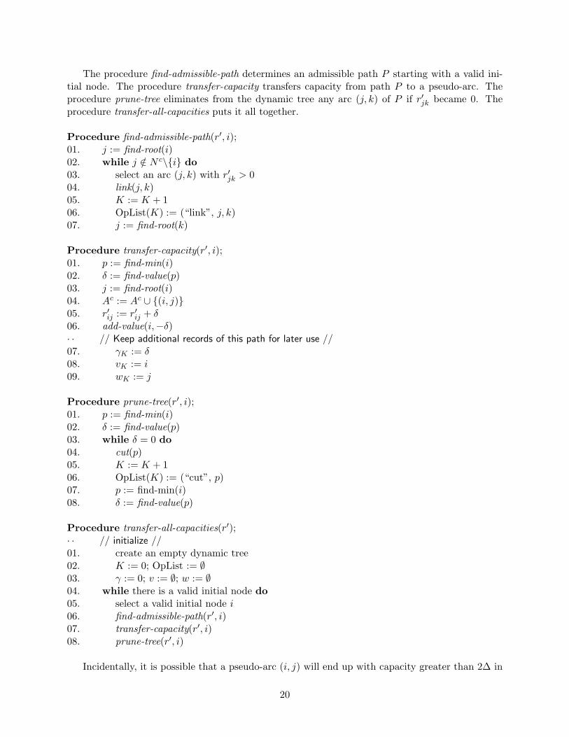
The procedure find-admissible-path determines an admissible path P starting with a valid ini-tial node. The procedure transfer-capacity transfers capacity from path P to a pseudo-arc. Theprocedure prune-tree eliminates from the dynamic tree any arc (j, k) of P if r′jk became 0. Theprocedure transfer-all-capacities puts it all together.

Procedure find-admissible-path(r′, i);01. j := find-root(i)02. while j /∈ N c\i do03. select an arc (j, k) with r′jk > 004. link(j, k)05. K := K + 106. OpList(K) := (“link”, j, k)07. j := find-root(k)

Procedure transfer-capacity(r′, i);01. p := find-min(i)02. δ := find-value(p)03. j := find-root(i)04. Ac := Ac ∪ (i, j)05. r′ij := r′ij + δ06. add-value(i,−δ)· · // Keep additional records of this path for later use //07. γK := δ08. vK := i09. wK := j

Procedure prune-tree(r′, i);01. p := find-min(i)02. δ := find-value(p)03. while δ = 0 do04. cut(p)05. K := K + 106. OpList(K) := (“cut”, p)07. p := find-min(i)08. δ := find-value(p)

Procedure transfer-all-capacities(r′);· · // initialize //01. create an empty dynamic tree02. K := 0; OpList := ∅03. γ := 0; v := ∅; w := ∅04. while there is a valid initial node do05. select a valid initial node i06. find-admissible-path(r′, i)07. transfer-capacity(r′, i)08. prune-tree(r′, i)

Incidentally, it is possible that a pseudo-arc (i, j) will end up with capacity greater than 2∆ in

20

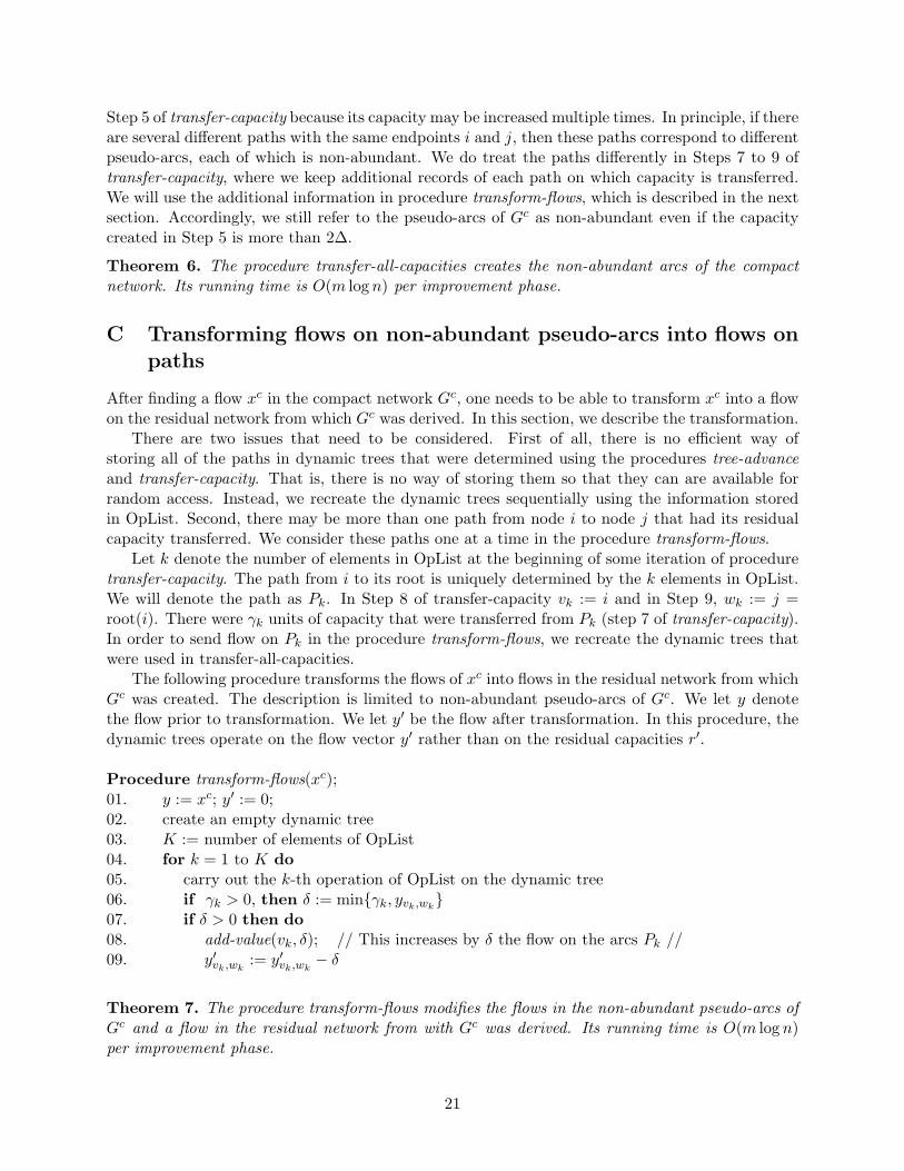
Step 5 of transfer-capacity because its capacity may be increased multiple times. In principle, if thereare several different paths with the same endpoints i and j, then these paths correspond to differentpseudo-arcs, each of which is non-abundant. We do treat the paths differently in Steps 7 to 9 oftransfer-capacity, where we keep additional records of each path on which capacity is transferred.We will use the additional information in procedure transform-flows, which is described in the nextsection. Accordingly, we still refer to the pseudo-arcs of Gc as non-abundant even if the capacitycreated in Step 5 is more than 2∆.

Theorem 6. The procedure transfer-all-capacities creates the non-abundant arcs of the compactnetwork. Its running time is O(m log n) per improvement phase.

C Transforming flows on non-abundant pseudo-arcs into flows onpaths

After finding a flow xc in the compact network Gc, one needs to be able to transform xc into a flowon the residual network from which Gc was derived. In this section, we describe the transformation.

There are two issues that need to be considered. First of all, there is no efficient way ofstoring all of the paths in dynamic trees that were determined using the procedures tree-advanceand transfer-capacity. That is, there is no way of storing them so that they can are available forrandom access. Instead, we recreate the dynamic trees sequentially using the information storedin OpList. Second, there may be more than one path from node i to node j that had its residualcapacity transferred. We consider these paths one at a time in the procedure transform-flows.

Let k denote the number of elements in OpList at the beginning of some iteration of proceduretransfer-capacity. The path from i to its root is uniquely determined by the k elements in OpList.We will denote the path as Pk. In Step 8 of transfer-capacity vk := i and in Step 9, wk := j =root(i). There were γk units of capacity that were transferred from Pk (step 7 of transfer-capacity).In order to send flow on Pk in the procedure transform-flows, we recreate the dynamic trees thatwere used in transfer-all-capacities.

The following procedure transforms the flows of xc into flows in the residual network from whichGc was created. The description is limited to non-abundant pseudo-arcs of Gc. We let y denotethe flow prior to transformation. We let y′ be the flow after transformation. In this procedure, thedynamic trees operate on the flow vector y′ rather than on the residual capacities r′.

Procedure transform-flows(xc);01. y := xc; y′ := 0;02. create an empty dynamic tree03. K := number of elements of OpList04. for k = 1 to K do05. carry out the k-th operation of OpList on the dynamic tree06. if γk > 0, then δ := minγk, yvk,wk

07. if δ > 0 then do08. add-value(vk, δ); // This increases by δ the flow on the arcs Pk //09. y′vk,wk

:= y′vk,wk− δ

Theorem 7. The procedure transform-flows modifies the flows in the non-abundant pseudo-arcs ofGc and a flow in the residual network from with Gc was derived. Its running time is O(m log n)per improvement phase.

21