arX

iv:0

912.

0108

v1 [

astr

o-ph

.SR

] 1

Dec

200

9

Modeling the Sun’s open magnetic flux and the heliospheric current sheet

J. Jiang, R. Cameron, D. Schmitt and M. Schussler

Max-Planck-Institut fur Sonnensystemforschung, 37191 Katlenburg-Lindau, Germany

jiang@mps.mpg.de

ABSTRACT

By coupling a solar surface flux transport model with an extrapolation of the he-

liospheric field, we simulate the evolution of the Sun’s open magnetic flux and the

heliospheric current sheet (HCS) based on observational data of sunspot groups since

1976. The results are consistent with measurements of the interplanetary magnetic field

near Earth and with the tilt angle of the HCS as derived from extrapolation of the ob-

served solar surface field. This opens the possibility for an improved reconstruction of

the Sun’s open flux and the HCS into the past on the basis of empirical sunspot data.

Subject headings: solar-terrestrial relations – Sun: activity – Sun: magnetic fields

1. Introduction

The Sun’s open magnetic flux is the part of its flux which is not contained in closed loops, but

extends into the heliosphere. It is the source of the heliospheric magnetic field (HMF) whose varia-

tions are an important source of geomagnetic activity (Pulkkinen 2007) and control the production

of cosmogenic isotopes by galactic cosmic rays (Beer 2000). A crucial feature of the HMF is the

heliospheric current sheet (HCS), the interface separating the opposite polarities of the HMF. The

tilt angle of the HCS (defined as the mean of the maximum northern and southern extensions of

the HCS) is a key parameter for the modulation of the flux of galactic cosmic rays in the inner he-

liosphere (Kota & Jokipii 1983; Ferreira & Potgieter 2004; Alanko-Huotari et al. 2007; Heber et al.

2009).

At a given distance from the Sun, the HMF has an almost uniform magnitude in latitude

and longitude (Balogh et al. 1995). Therefore, its radial component near Earth, which has been

measured by spacecraft since the 1960s, faithfully represents the Sun’s total open flux (Owens et al.

2008; Lockwood et al. 2009). The tilt angle of the HCS could, in principle, be measured by multiple

spacecraft orbiting at different heliolatitudes. However, with the exception of the Ulysses probe, all

measurements of the HMF have been obtained near the ecliptic plane, so that direct measurements

of the tilt angle of the HCS are not available most of the time. Therefore, such data are derived

by extrapolation of solar surface field maps, such as those taken at the Wilcox Solar Observatory

(WSO) since 1976. This yields the current sheet distribution at the source surface, where the field

– 2 –

is assumed to become radial (e.g., Hoeksema et al. 1982). In the inner heliosphere, we may ignore

dynamical effects such as the acceleration of slow plasma and the deceleration of fast plasma that

occur when neighboring parcels of plasma interact (Riley et al. 2002), so the field lines are assumed

to stay purely radial beyond the source surface. Under these conditions, the morphology of the

HCS may be inferred from the position of the current sheet at the source surface.

A limitation of this semi-empirical determination of the HCS tilt angle arises from the de-

creasing reliability of the surface field measurements at higher latitudes and from magnetographic

saturation effects, which cannot be corrected without further assumptions. Flux transport mod-

els based upon observed large-scale magnetic flux emergence (e.g., in sunspot groups) provide a

complementary possibility to obtain information about the high-latitude surface fields, which con-

trol the open flux and the HCS tilt angle during solar minimum periods (e.g. Wang et al. 1989a,

2000; Mackay et al. 2002). Schussler & Baumann (2006) showed that such an approach reproduces

well the HMF over multiple solar cycles, provided that the heliospheric current sheet is explicitly

included in the field extrapolation (current sheet source surface method, cf. Zhao & Hoeksema

1995a)

The present paper serves a two-fold purpose. Firstly, it extends the study of Schussler & Baumann

(2006) until the current solar minimum period and includes an explicit account of the HCS and its

tilt angle, which can be compared with the corresponding observational quantities. Secondly, such

comparison provides the validation for the application of these methods to reconstruct the open

flux and HCS tilt angle backward in time.

The paper is organized as follows. In Sect. 2, we give the description of the models used. The

results are presented in Sect. 3: photospheric flux distributions in Sect. 3.1, the solar open flux in

Sect. 3.2, and the heliospheric current sheet in Sect. 3.3. We give our conclusions in Sect. 4.

2. Methods

2.1. Surface flux transport model

The surface flux transport (SFT) model describes the evolution of the magnetic flux distribu-

tion at the solar surface as a combined result of the emergence of bipolar magnetic regions (BMRs),

flux cancellation, and transport by surface flows. The evolution of the radially orientated surface

field (Wang & Sheeley 1992; Solanki 1993; Petrie & Patrikeeva 2009) is controlled by latitudinal

differential rotation and meridional flow, together with turbulent diffusion due to granulation and

supergranulation (e.g., Wang et al. 1989b; Mackay et al. 2002).

The SFT uses the radial component of the induction equation in the form

∂Br

∂t= − ω(θ)

∂Br

∂φ− 1

R⊙ sin θ

∂

∂θ[υ(θ)Br sin θ]

– 3 –

+ηh

R2⊙

[

1

sin θ

∂

∂θ

(

sin θ∂Br

∂θ

)

+1

sin2 θ

∂2Br

∂φ2

]

− Dr(ηrB) + S(θ, φ, t), (1)

where S(θ, φ, t) is the source term describing the emergence of new magnetic flux and Dr(ηrB)

is the decay term parameterizing the radial diffusion of the magnetic field (Baumann et al. 2006).

Following Jiang et al. (2009), the horizontal diffusivity ηh and radial diffusivity ηr are taken as

600 km2 s−1 and 100 km2 s−1, respectively. For the meridional flow υ(θ), we adopt the profile

υ(θ) =

−υ0 sin(2.4 ∗ (90 − θ)) 15 ≤ θ ≤ 165

0 otherwise,(2)

where υ0 = 11 m s−1. This profile is largely consistent with helioseismic results (Gizon & Duvall

2004). For the latitudinal differential rotation ω(θ), we use the empirical profile determined by

Snodgrass (1983).

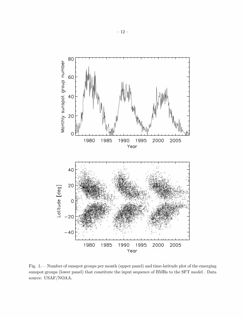
The basis for magnetic flux input to the SFT model by emerging BMRs is the USAF/NOAA

sunspot group record 1. Since a sunspot group typically appears more than once in the record, we

consider a group only at the day of its maximum area. Figure 1 gives the monthly number and the

latitude distribution (butterfly diagram) of the emerging sunspot groups for the time interval 1976

– 2009, which provide the flux input for the SFT model.

The observed sunspot areas have been converted to the areas of the corresponding BMRs

following the procedure of Baumann et al. (2004). We include the magnetic flux contained in

faculae and plages by employing the statistical relationship between sunspot area, As, and facular

area, Af , determined by Chapman et al. (1997),

Af = 414 + 21As − 0.0036A2s , (3)

(in units of millionths of the solar hemisphere) and take ABMR = As +Af as area of the correspond-

ing BMR. Since there is no information about the magnetic polarity in the USAF/NOAA data,

we use Hale’s polarity law to infer the polarities of the leading and following parts of the BMRs.

We resolve the ambiguity arising from the overlap of cycles around activity minima by assuming

that BMRs emerging below ±15 latitude during the overlap period belong to the old cycle while

all others belong to the new cycle. The angular separation, ∆β (in degrees), between the leading

and following polarity patches of a BMR is assumed to be proportional to the square root of the

BMR area (given in square degrees): ∆β = 0.6√

ABMR. The angular separation is separated into

latitudinal and longitudinal components, depending on the BMR tilt angle, γ, with respect to the

E–W direction. We assume the relation γ = 0.15λ , which is consistent with observational results

1http://solarscience.msfc.nasa.gov/greenwch.shtml

– 4 –

(Howard 1991; Sivaraman et al. 1999, Dasi Espuig et al., in preparation)2. Finally, we calibrate the

conversion factor between BMR area and magnetic flux by matching the observed and simulated

values of the disk-averaged unsigned flux density, Bs =∫ ∫

| Br | dφ cos(λ)dλ/4π.

2.2. Field extrapolation model

In order to determine the coronal and heliospheric magnetic field from its source in the photo-

spheric field, a field extrapolation method is required. For the field distribution on a global scale,

the most widely used approach is the potential field source surface (PFSS) model (Schatten et al.

1969; Altschuler & Newkirk 1969). However, the PFSS model (which includes only volume currents

beyond the spherical source surface, where the field is assumed to become purely radial) does neither

reproduce the latitude-independent radial field found with Ulysses (Balogh et al. 1995) nor does

it match the measured interplanetary radial field near Earth (Schussler & Baumann 2006). The

current sheet source surface (CSSS) model (Zhao & Hoeksema 1995a,b; Zhao et al. 2002), which

explicitly takes into account the existence of the HCS, does not suffer from these deficiencies and

provides a reasonable match to the measured quantities (Schussler & Baumann 2006).

We briefly describe the main features of the CSSS model as follows. To include the effects of

volume and sheet currents, the exterior of the Sun is divided into three parts, which are separated by

two spherical surfaces, the cusp surface at r = Rcs, and the source surface at r = Rss (Rcs < Rss).

In the region inside the cusp surface, the field is potential. In the region between Rcs and Rss,

all flux loops are reconfigured with volume currents and current sheets, so that the field becomes

completely open. In the region beyond Rss, the field is purely radial. Apart from Rcs and Rss,

the third adjustable parameter of the CSSS model is the height scale, a, of the horizontal current.

Following Zhao et al. (2002), we take a = 0.2R⊙ in our calculations. We choose Rss = 10.0R⊙

according to the estimate of Marsch & Richter (1984). The value of Rcs = 1.8R⊙ is determined by

the comparison between the magnetic flux at the cusp surface and the measured radial field from

OMNI2 data in Sect. 3.2.

Technically, the opening of the flux beyond Rcs and the introduction of the current sheet(s)

is carried out by first calculating a global potential-field extrapolation for the entire volume above

the solar surface. The unsigned radial component of the field at the cusp surface is then used as

the boundary condition for calculating a magnetic field distribution between Rcs and Rss of the

form in Bogdan & Low (1986) and used by Zhao & Hoeksema (1995a). The orientation of the field

2Schussler & Baumann (2006) attempted to fix the latitude-dependence of the tilt angle independently by cali-

brating with the longitude-averaged surface field integrated over latitude, viz.R

|R

Brdφ | cos(λ)dλ/4π. However,

some exploratory experiments we performed have shown that this quantity is rather sensitive to the observed scatter

of the BMR tilt angles about the latitude-dependent mean. Since the effect of this scatter is not significant for the

quantities that we study in this paper (open flux and tilt of the heliospheric current sheet), we do not consider BMR

tilt angle fluctuations here.

– 5 –

lines is then changed where necessary so that the sign and magnitude of the radial field at Rcs is

continuous. The distribution of the field outside Rcs can then be determined.

3. Results

3.1. Photospheric magnetic field distributions

The initial condition for the photospheric flux distribution is the same as the one assumed

by Baumann et al. (2004). It satisfies an approximate balance between the effects of poleward

meridional flow and equatorial diffusion (van Ballegooijen et al. 1998). The memory of the system

regarding the initial field depends on the value of the radial diffusion parameter, ηr (Baumann et al.

2006). We use ηr = 100 km2 s−1, which leads to a memory of about 20 yrs. We start all our

simulations from the beginning of the USAF/NOAA sunspot group record in 1874, but consider

the results only for the time period 1976–2009. Therefore, there is no remaining influence of the

initial fields on the results presented below.

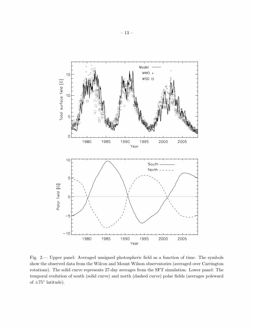
The upper panel of Fig. 2 shows a comparison of observed and simulated time evolution of the

averaged unsigned flux density at the solar surface, Bs (defined in Sec. 2.1), which has been used to

calibrate the relation between area and magnetic flux of the BMRs providing the input for the flux

transport model. Note that, without any other parameter adjustment, the model reproduces well

the ratio between the maximum and minimum values as well as the very low surface flux during

the current minimum.

The lower panel of Fig. 2 gives the corresponding time evolution of the high-latitude surface

field, averaged over the caps poleward of ±75 latitude. The field amplitude and reversal times

before 2002 are consistent with the observational results given by Arge et al. (2002). For the current

minimum, the reported values of the polar field do not give a consistent picture, reflecting the

difficulties and limitations of polar field measurement. Petrie & Patrikeeva (2009) obtained polar

fields of 5 – 6 G by analyzing photospheric and chromospheric vector polarimetric data obtained

with SOLIS at NSO, which is consistent with our model. On the other hand, MWO magnetograph

(Svalgaard et al. 2005) data and more indirect indices (Schatten 2005) suggest that the present

polar field could possibly be a factor 2 smaller than that during the previous activity minimum

around 1997 (see further discussion in Sect. 3.4).

3.2. Open flux and near-Earth radial field

We can calculate the total open flux Φopen resulting from our extrapolation model by integrat-

ing the unsigned radial magnetic field over the source surface, viz.

Φopen(t) = R2ss

∫ ∫

|Br(Rss, λ, φ)|dΩ. (4)

– 6 –

Actually, in the CSSS model the open flux is already fixed at the cusp surface, Rcs, smaller values

of which leading to a larger amount of open flux. In order to compare with data provided by

near-Earth measurements, we also calculate the longitudinally averaged unsigned radial field near

Earth (at rE = 1 AU and λ = 0, thus ignoring the slight variation due to the angle of about 7

degrees between the equatorial plane of the Sun and the ecliptic plane),

BE(t) =1

2π

(

Rss

rE

)2 ∫ 2π

0

|Br (Rss, 0, φ, t) | dφ . (5)

Since extrapolations with the CSSS model reproduce the latitude-independence of the radial field

at r = rE (Schussler & Baumann 2006), we have BE ≃ Φopen/(4πr2E) to a high degree of accuracy,

so that BE also represents the open flux. Similarly, it has been shown that, possibly after some

correction for kinematical effects due to the solar wind, the measured radial field near Earth can

be taken as a reliable proxy for the total open flux (Owens et al. 2008; Lockwood et al. 2009).

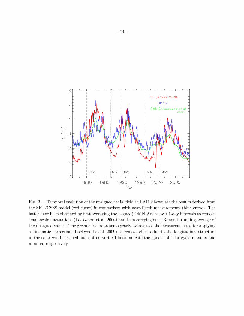
Figure 3 shows 27-day averages of BE from our combined SFT/CSSS model (with Rcs = 1.8R⊙,

Rss = 10R⊙, a = 0.2R⊙, red curve) in comparison with the measured radial field from OMNI2 data

(blue curve) 3. Lockwood et al. (2009) have suggested that the observed data better represent the

open flux of the Sun if a correction of kinematical effects due to the longitudinal structure of the

solar wind is applied. Data modified in this way are also shown in Fig. 3 (green curve).

The phase relation between the solar activity cycle and the near-Earth field (and thus the open

flux) is well represented by our model, with BE reaching its peak values ∼ 2 – 3 yr after activity

maximum (cf. Mackay et al. 2002; Wang et al. 2002; Schussler & Baumann 2006). Including the

diffusion in radial direction in the SFT model and the realistic tilt angles of BMRs with respect to

the E–W direction are the main reasons that lead to the correct phase relation. The only periods

showing a significant disagreement between our model and the data are the ascending phases of the

activity cycles, where the model values are too low. Possibly the model misses open flux from small

coronal holes at intermediate latitude during this phase. In principle, this could be corrected by

putting the cusp surface nearer to the Sun during this cycle phase or by assuming a non-spherical

cusp surface. The amplitude of the variation of BE is also affected by the value of radial diffusion

in the SFT model. However, such parameter tuning would not provide further physical insight

while the overall agreement between model and data is already encouraging and sufficient for the

purposes of this paper.

3.3. Heliospheric current sheet (HCS)

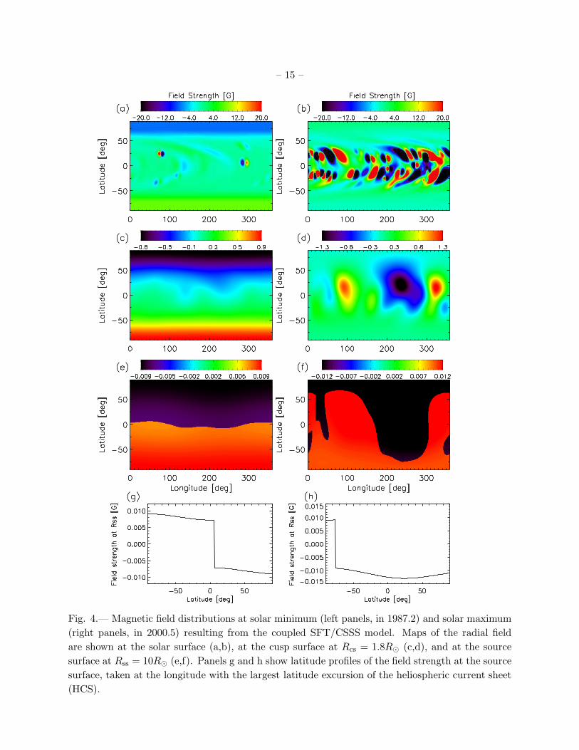
Figure 4 shows the distributions of the magnetic field on the solar surface, on the cusp surface,

and on the source surface during typical solar minimum and solar maximum conditions in our

3http://omniweb.gsfc.nasa.gov/

– 7 –

coupled SFT/CSSS model. Around solar minimum (left panels), the field at (and outward of) the

source surface assumes a ‘split-monopole’ structure (Banaszkiewicz et al. 1998), the HCS separating

the two polarities being located near the equatorial plane (Hu et al. 2008). Near activity maximum

(right panels), the HCS shows strong excursions in latitude and additional localized current sheets

may occur. Apart from the current sheets, the field is always largely latitude-independent. The tilt

angle of the HCS is defined by convention as the arithmetic mean of the maximum northward and

southward excursions of the HCS (see http://wso.stanford.edu/Tilts.html). At the moments shown

in Fig. 4, the HCS tilt angle is 6.5 in the activity minimum period and 71.3 in the maximum

period.

A comparison between the tilt angle of the HCS resulting from our SFT model with the values

derived by PFSS extrapolations of WSO maps of the surface magnetic field is shown in Fig. 5a.

The results from our standard CSSS extrapolation (solid red line) do not significantly deviate from

those obtained by a PFSS extrapolation of the same SFT results with Rss = 3.25R⊙ (dashed red

line), suggesting that the calculated tilt angle does not sensitively depend on the extrapolation

method (in contrast to the distribution of open flux). The other two curves in Fig. 5a represent

PFSS extrapolations based on observed photospheric magnetic fields using two different boundary

conditions for the photospheric magnetic field (see http://wso.stanford.edu/Tilts.html). Both the

‘classic’ (green curve) and ‘new’ (blue curve) extrapolations provided by the WSO website assume

that the field is potential between the photosphere and the source surface. The two models differ

in the way the photospheric field observations are used as the inner boundary condition and in the

height of the source surface. In the ‘classic’ case the surface observations are taken to correspond

to the line-of-sight component of the potential field, and the source surface is assumed to be at 2.5

R⊙. In the ‘new’ model, the observed field is matched to the radial component of the potential

field projected onto the line of sight: the assumption is that the field in the photosphere is purely

radial and becomes potential only above the surface. Extrapolation for the ‘new’ case exist on the

WSO website for source surface heights of 2.5 R⊙ and 3.25 R⊙. We show the result for 3.25 R⊙

which is claimed to better match Ulysses data.

The result from our model is consistent with both extrapolations. Figure 5b shows the dif-

ference between the HCS tilt angle derived from the SFT model with CSSS extrapolation and the

other three cases. The agreement with the WSO ‘new’ method is somewhat worse than that of

the ‘classic’ method, especially around the activity minimum periods. For physical reasons, it is

expected that the ‘new’ method assuming a purely radial photospheric field should be a better

representation of the real solar situation (Wang & Sheeley 1992; Petrie & Patrikeeva 2009). Note,

however, that inferring the radial field strength from the measured line-of-sight component requires

quite large corrections factors at high solar latitudes together with the larger uncertainties of the

high-latitude data. This suggests that the tilt angles derived from observed synoptic maps during

solar minimum periods should be considered with some caution.

– 8 –

3.4. The minimum of cycle 23

The current solar minimum appears to be rather extended, with particularly low activity levels.

There are indications that the polar field strength is significantly lower than during the two previous

minima (e.g. Svalgaard et al. 2005; Schatten 2005; Schrijver & Liu 2008). A low polar field strength

would be consistent with the small measured values of the near-Earth interplanetary magnetic field

(and thus also the open flux, see Fig. 3) and the relatively large tilt angle of the HCS inferred by

the ‘classic’ PFSS extrapolation (blue curve in Fig. 5a). However, the uncertainties in the inferred

values of the polar field are large and the HCS tilt angle determined with the (presumably more

relevant) ‘new’ PFSS model using a radial-field photospheric boundary condition does not show

unusually large minimum values.

Our SFT model yields a polar field during the present minimum which is is not significantly

weaker than that of the previous minimum (see Fig. 2). The open flux determined from the model

is consistent with the low OMNI2 measurements during the current minimum; however, the model

results tend to be too low during minima, so that the present agreement might well be fortuitous.

The tilt angle of the HCS derived from the SFT model decreases to low values during the current

minimum, which is consistent with the ‘normal’ polar field strength that the model yields. The

tilt angles inferred from PFSS extrapolations based on observed photospheric field distributions

provide a confusing picture (cf. Fig. 5a): while the ‘classic’ line-of-sight boundary condition leads

rather large tilt angles, which would be in accordance with a weak polar field, the ‘new’ radial-field

boundary condition predicts values not much different from those during previous cycles. As the

‘new’ method is considered to be physically more realistic (Petrie & Patrikeeva 2009), this would

dilute the case for an unusually weak polar field during the present minimum.

In the SFT model, the magnitude reached by the polar field in the second half of a cycle

crucially depends on the tilt angle (with respect to the East-West direction) of the emerging bipolar

magnetic regions during the cycle. We have assumed the same relationship, γ = 0.15λ, between tilt

angle and emergence latitude for all cycles considered. However, the analysis of sunspot group data

indicates that the factor of proportionality in this relation may actually vary from cycle to cycle

(Dasi Espuig et al., in preparation). Systematically smaller tilt angles during cycle 23 could lead

to a unusually weak polar field during the present minimum. Alternatively, Schrijver & Liu (2008)

proposed an increased strength of the diverging meridional flow near the equator as an explanation

for the weak polar field.

4. Conclusions

We have simulated the temporal evolution of the Sun’s total open magnetic flux and the

heliospheric current sheet (HCS) since 1976 by coupling a surface flux transport (SFT) model and

the current sheet source surface (CSSS) extrapolation method, using the observed sunspot groups

to provide the magnetic flux input for the model. We draw the following conclusion from our

– 9 –

results:

1) The simulated open flux matches the OMNI2 data quite well, except for systematically

lower values in the ascending phase of the activity cycle. This is consistent with the view that the

solar open flux is largely determined by the instantaneous photospheric sources.

2) At the source surface, the magnetic field satisfies the ‘split monopole’ configuration suggested

by the Ulysses out-of-ecliptic measurements.

3) The temporal variation of the tilt angle of the HCS from the SFT/CSSS model matches the

values derived from potential field source surface(PFSS) extrapolations of the observed photospheric

magnetic field. The best agreement is found for the ‘classic’ line-of-sight condition.

4) The conditions during the present minimum period of cycle 23 as provided by the SFT/CSSS

model are similar to those at previous minima: the polar field has about the same strength as that

of cycle 22, the tilt angle of the HCS is small, and the open flux is roughly at the level of the last

minimum. Since 2007, however, the HCS tilt angle has deviated significantly from the WSO PFSS

values with line-of-sight boundary condition (‘classic’ case) and approached those with the ‘new’

radial boundary condition. These results may well be affected by a systematic variations of the

sunspot group tilts with respect to the E–W direction from cycle to cycle, as indicated by recent

analysis of sunspot observations.

5) In spite of some deviations in detail, the overall agreement of the model results with ob-

servationally inferred values of open flux and current sheet geometry is encouraging. It opens the

possibility to extend the model backward in time by using the sunspot group record since 1874.

This will be the topic of a subsequent paper.

Acknowledgments: Y.-M. Wang kindly provided the observational datasets of the averaged

unsigned photospheric field shown in Fig. 2. M. Lockwood kindly provided the kinematically

corrected OMNI2 data shown in Fig. 3.

REFERENCES

Alanko-Huotari, K., Usoskin, I. G., Mursula, K., & Kovaltsov, G. A. 2007, Adv. Space Res., 40,

1064

Altschuler, M. D., & Newkirk, G. 1969, Sol. Phys., 9, 131

Arge, C. N., Hildner, E., Pizzo, V. J., & Harvey, J. W. 2002, J. Geophys. Res., 107, 1319

Balogh, A., Smith, E. J., Tsurutani, B. T., Southwood, D. J., Forsyth, R. J., & Horbury, T. S.

1995, Science, 268, 1007

Banaszkiewicz, M., Axford, W. I., & McKenzie, J. F. 1998, A&A, 337, 940

– 10 –

Baumann, I., Schmitt, D., Schussler, M., & Solanki, S. K. 2004, A&A, 426, 1075

Baumann, I., Schmitt, D., & Schussler, M. 2006, A&A, 446, 307

Beer, J. 2000, Space Sci. Rev., 94, 53

Bogdan, T. J., & Low, B. C. 1986, ApJ, 306, 271

Chapman, G. A., Cookson, A. M., & Dobias, J. J. 1997, ApJ, 482, 541

Ferreira, S. E. S., & Potgieter, M. S. 2004, ApJ, 603, 744

Gizon, L. & Duvall, T. L. 2004, in Multi-Wavelength Investigations of Solar Activity, ed. Stepanov,

A. V., Benevolenskaya, E. E., & Kosovichev, A. G., IAU Symp., 223, 41

Heber, B., Kopp, A., Gieseler, J., Muller-Mellin, R., Fichtner, H., Scherer, K., Potgieter, M. S., &

Ferreira, S. E. S. 2009, ApJ, 699, 1956

Hoeksema, J. T., Wilcox, J. M., & Scherrer, P. H. 1982, J. Geophys. Res., 87, 10331

Howard, R. F. 1991, Sol. Phys., 136, 251

Hu, Y. Q., Feng, X. S., Wu, S. T., & Song, W. B. 2008, J. Geophys. Res., 113, A03106

Jiang, J, Cameron, R., Schmitt, D., & Schussler, M. 2009, ApJ, 693, L96

Kota, J., & Jokipii, J. R. 1983, ApJ, 265, 573

Leighton, R. B. 1964, ApJ, 140, 1547

Lockwood, M., Rouillard, A. P., Finch, I., & Stamper, R. 2006, J. Geophys. Res., 111, A09109

Lockwood, M., Rouillard, A. P., & Finch, I. D. 2009, ApJ, 700, 937

Mackay, D. H., Priest, E. R., & Lockwood, M. 2002, Sol. Phys., 209, 287

Marsch, E., & Richter, A. K. 1984, J. Geophys. Res., 89, 5386

Owens, M. J., Arge, C. N., Crooker, N. U., Schwadron, N. A., & Horbury, T. S. 2008, J. Geophys.

Res., 113, 12103

Petrie, G. J. D., & Patrikeeva, I. 2009, ApJ, 699, 871

Pulkkinen, T. 2007, Living Rev. Solar Phys., 1, 4

Riley, P., Linker, J. A., & Mikic, Z. 2002, J. Geophys. Res., 107, 1136

Schatten, K., 2005, Geophys. Res. Lett., 32, 21106

Schatten, K. H., Wilcox, J. M., & Ness, N. F. 1969, Sol. Phys., 6, 442

– 11 –

Schussler, M., & Baumann, I. 2006, A&A, 459, 945

Schrijver, C. J., & Liu, Y. 2008, Sol. Phys., 252, 19

Sivaraman, K. R., Gupta, S. S., & Howard, R. F. 1999, Sol. Phys., 189, 69

Snodgrass, H. B. 1983, ApJ, 501, 866

Solanki, S. K., 1993, Space Sci. Rev., 63, 1

Svalgaard, L., Cliver, E. W. & Kamide, Y. 2005, Geophys. Res. Lett., 32, L01104

van Ballegooijen, A. A., Cartledge, N. P., & Priest, E. R., 1998, ApJ, 501, 866

Wang, Y.-M., Nash, A. G., & Sheeley, N. R., Jr. 1989a, Sol. Phys., 347, 529

Wang, Y.-M., Nash, A. G., & Sheeley, N. R., Jr. 1989b, Science, 245, 712

Wang, Y.-M., & Sheeley, N. R., Jr. 1992, ApJ, 392, 310

Wang, Y.-M, Sheeley, N. R., Jr., & Lean, J. 2000, Geophys. Res. Lett., 27, 621

Wang, Y.-M., Sheeley, N. R., Jr., & Lean, J. 2002, ApJ, 580, 1188

Zhao, X. P., Hoeksema, J. T. 1995a, J. Geophys. Res., 100, 19

Zhao, X. P., Hoeksema, J. T. 1995b, Space Sci. Rev., 72, 189

Zhao, X. P., Hoeksema, J. T., & Rich, N. R. 2002, Adv. Space Res., 29, 411

This preprint was prepared with the AAS LATEX macros v5.2.

– 12 –

Fig. 1.— Number of sunspot groups per month (upper panel) and time-latitude plot of the emerging

sunspot groups (lower panel) that constitute the input sequence of BMRs to the SFT model . Data

source: USAF/NOAA.

– 13 –

Fig. 2.— Upper panel: Averaged unsigned photospheric field as a function of time. The symbols

show the observed data from the Wilcox and Mount Wilson observatories (averaged over Carrington

rotations). The solid curve represents 27-day averages from the SFT simulation. Lower panel: The

temporal evolution of south (solid curve) and north (dashed curve) polar fields (averages poleward

of ±75 latitude).

– 14 –

Fig. 3.— Temporal evolution of the unsigned radial field at 1 AU. Shown are the results derived from

the SFT/CSSS model (red curve) in comparison with near-Earth measurements (blue curve). The

latter have been obtained by first averaging the (signed) OMNI2 data over 1-day intervals to remove

small-scale fluctuations (Lockwood et al. 2006) and then carrying out a 3-month running average of

the unsigned values. The green curve represents yearly averages of the measurements after applying

a kinematic correction (Lockwood et al. 2009) to remove effects due to the longitudinal structure

in the solar wind. Dashed and dotted vertical lines indicate the epochs of solar cycle maxima and

minima, respectively.

– 15 –

Fig. 4.— Magnetic field distributions at solar minimum (left panels, in 1987.2) and solar maximum

(right panels, in 2000.5) resulting from the coupled SFT/CSSS model. Maps of the radial field

are shown at the solar surface (a,b), at the cusp surface at Rcs = 1.8R⊙ (c,d), and at the source

surface at Rss = 10R⊙ (e,f). Panels g and h show latitude profiles of the field strength at the source

surface, taken at the longitude with the largest latitude excursion of the heliospheric current sheet

(HCS).

– 16 –

Fig. 5.— (a) Temporal evolution of the HCS tilt angle. Solid red curve: SFT result with CSSS

extrapolation (a = 0.2R⊙, Rcs=1.8R⊙,Rss=10R⊙); dashed red curve: SFT result with PFSS extrapola-

tion (Rss = 3.25R⊙); blue curve: PFSS extrapolation of WSO synoptic maps with line-of-sight field

boundary condition (‘classic’ model, Rss = 2.5R⊙); green curve: PFSS extrapolation of WSO syn-

optic maps with radial field boundary condition (‘new’ model, Rss = 3.25R⊙). The data for the blue

and green curves have been obtained from the WSO website (http://wso.stanford.edu/Tilts.html).

(b) The difference between the HCS tilt angle from the SFT/CSSS and the three other methods

shown in the same color scheme as used in (a).