Embed Size (px)
Citation preview
Max-Plus Algebra
Kasie G. Farlow
Master’s Thesis submitted to the Faculty of the
Virginia Polytechnic Institute and State University
in partial fulfillment of the requirements for the degree of
Masters
in
Mathematics
Dr. Martin Day, Chair
Dr. Peter Haskell,
Dr. Robert Wheeler
April 27, 2009
Blacksburg, Virginia
Keywords: Max-Plus, Linear Algebra, Markov Chains
Copyright 2009, Kasie G. Farlow
Max-Plus Algebra
Kasie G. Farlow
(Abstract)
In max-plus algebra we work with the max-plus semi-ring which is the set Rmax = {−∞}∪R
together with operations a⊕ b = max(a, b) and a⊗ b = a+ b. The additive and multiplica-
tive identities are taken to be ε = −∞ and e=0 respectively. Max-plus algebra is one of
many idempotent semi-rings which have been considered in various fields of mathematics.
Max-plus algebra is becoming more popular not only because its operations are associative,
commutative and distributive as in conventional algebra but because it takes systems that
are non-linear in conventional algebra and makes them linear. Max-plus algebra also arises
as the algebra of asymptotic growth rates of functions in conventional algebra which will
play a significant role in several aspects of this thesis. This thesis is a survey of max-plus
algebra that will concentrate on max-plus linear algebra results. We will then consider from
a max-plus perspective several results by Wentzell and Freidlin for finite state Markov chains
with an asymptotic dependence.
Contents
Abstract ii
Table Of Contents iii
List of Figures v
1 Introduction 1
1.1 Brief History . . . . . . . . . . . . . . . . . . . . . . . . . . . . . . . . . . . 1
1.2 Definitions and Basic Algebraic Properties . . . . . . . . . . . . . . . . . . . 8
1.3 Matrices and Vectors in Max Plus Algebra . . . . . . . . . . . . . . . . . . . 11
1.3.1 Matrices . . . . . . . . . . . . . . . . . . . . . . . . . . . . . . . . . . 11
1.3.2 Vectors . . . . . . . . . . . . . . . . . . . . . . . . . . . . . . . . . . . 13
1.4 Max-Plus and Graph Theory . . . . . . . . . . . . . . . . . . . . . . . . . . . 13
2 Max-Plus Linear Algebra 18
2.1 Inverse Matrices . . . . . . . . . . . . . . . . . . . . . . . . . . . . . . . . . . 18
2.2 Determinants . . . . . . . . . . . . . . . . . . . . . . . . . . . . . . . . . . . 23
iii

2.3 Linear Systems . . . . . . . . . . . . . . . . . . . . . . . . . . . . . . . . . . 26
2.3.1 Principal Sub-Solution . . . . . . . . . . . . . . . . . . . . . . . . . . 26
2.3.2 Cramer’s Rule . . . . . . . . . . . . . . . . . . . . . . . . . . . . . . . 28
2.3.3 Solving x = (A⊗ x) ⊕ b . . . . . . . . . . . . . . . . . . . . . . . . . 31
2.4 Eigenvalue and Eigenvectors . . . . . . . . . . . . . . . . . . . . . . . . . . . 32
2.5 Cayley-Hamilton and the Max-Plus Characteristic Equation . . . . . . . . . 45
2.6 Linear Dependence and Independence . . . . . . . . . . . . . . . . . . . . . . 51
2.6.1 Bases . . . . . . . . . . . . . . . . . . . . . . . . . . . . . . . . . . . . 52
2.7 Asymptotic and Limiting Behavior . . . . . . . . . . . . . . . . . . . . . . . 53
3 Markov Chains 61
3.0.1 Problem 1 . . . . . . . . . . . . . . . . . . . . . . . . . . . . . . . . . 63
3.0.2 Problem 2 . . . . . . . . . . . . . . . . . . . . . . . . . . . . . . . . . 72
3.0.3 Problem 3 . . . . . . . . . . . . . . . . . . . . . . . . . . . . . . . . . 77
4 Concluding Remarks 80
Bibliography 81
List of Symbols 85
iv
List of Figures
1.1 Train problem . . . . . . . . . . . . . . . . . . . . . . . . . . . . . . . . . . . 3
3.1 G(U1) . . . . . . . . . . . . . . . . . . . . . . . . . . . . . . . . . . . . . . . 66
3.2 G(U2) . . . . . . . . . . . . . . . . . . . . . . . . . . . . . . . . . . . . . . . 68
3.3 G(U3) . . . . . . . . . . . . . . . . . . . . . . . . . . . . . . . . . . . . . . . 75
v
Chapter 1
Introduction
1.1 Brief History
In max-plus algebra we work with the max-plus semi-ring which is the set Rmax = {−∞}∪R
together with operations a⊕b = max(a, b) and a⊗b = a+b. The additive and multiplicative
identities are taken to be ε = −∞ and e = 0 respectively. Its operations are associative,
commutative and distributive as in conventional algebra.
Max-plus algebra is one of many idempotent semi-rings which have been considered in vari-
ous fields of mathematics. One other is min-plus algebra. There ⊕ means minimum and the
additive identity is ∞. See [26] for other examples. We will only be concerned with max-plus
algebra. It first appeared in 1956 in Kleene’s paper on nerve sets and automata [18],[15].
It has found applications in many areas such as combinatorics, optimization, mathematical
physics and algebraic geometry [15]. It is also used in control theory, machine scheduling,
discrete event processes, manufacturing systems, telecommunication networks, parallel pro-
cessing systems and traffic control, see [7], [12] and [9]. Many equations that are used to
describe the behavior of these applications are nonlinear in conventional algebra but become
linear in max-plus algebra. This is a primary reason for its utility in various areas [7].
1
Kasie G. Farlow Chapter 1. Introduction 2
Many of the theorems and techniques we use in classical linear algebra have analogues in
the max-plus semi-ring. Cunningham-Green, Gaubert, Gondran and Minoux are among the
researchers who have devoted a lot of time creating much of the max-plus linear algebra
theory we have today. Many of Cunningham-Greens’ results are found in [9]. They have
studied concepts such as solving systems of linear equations, the eigenvalue problem, and
linear independence in the max-plus sense. In Chapter 2 we will see the extent to which max-
plus algebra is an analogue of classical linear algebra and look at many max-plus counterparts
of conventional results.
To illustrate the usefulness of max-plus algebra in a simple example, let’s look at a railroad
network between two cities. A similar example can be found in [16]. This is an example of
how max-plus algebra can be applied to a discrete event system. Assume we have two cities
such that S1 is the station in the first city, and S2 is the station in the second city. This
system contains 4 trains. The time it takes a train to go from S1 to S2 is 3 hours where the
train travels along track 1. It takes 2 hours to go from S2 to S1 where the train travels along
track 2. These tracks can be referred to as the long distance tracks. There are two more
tracks in this network, one which runs through city 1 and one which runs through city 2.
We can refer to these as the inner city tracks. Call them tracks 3 and 4 respectively. We can
picture track 3 as a loop beginning and ending at S1. Similarly, track 4 starts and ends at
S2. The time it takes to traverse the loop on track 3 is 2 hours. The time it takes to travel
from S2 to S2 on track 4 is 4 hours. Track 3 and track 4 each contain a train. There are
two trains that circulate along the two long distance tracks. In this network we also have
the following criteria:
1. The travel times along each track indicated above are fixed
2. The frequency of the trains must be the same on all four tracks
3. Two trains must leave a station simultaneously in order to wait for the changeover of
passengers

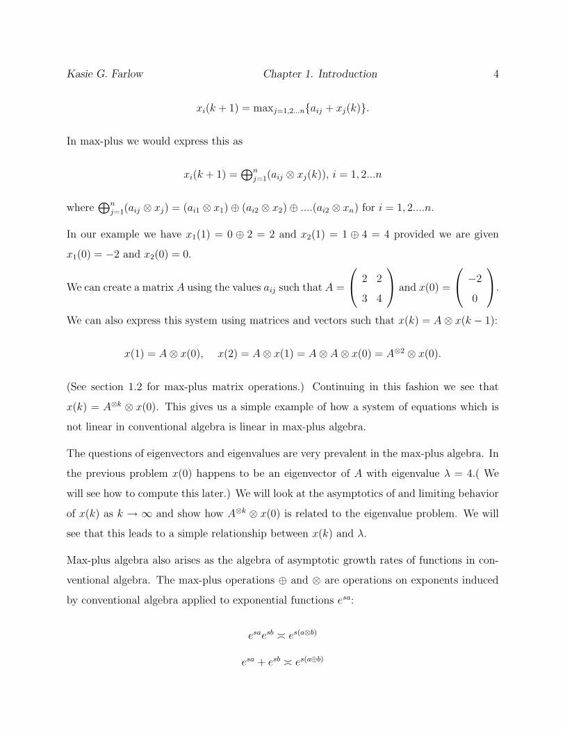
Kasie G. Farlow Chapter 1. Introduction 3
4. The two (k + 1)st trains leaving Si can not leave until the kth train that left the other
station arrives at Si.
xi(k− 1) will denote the the kth departure time for the two trains from station i. Therefore
x1(k) denotes the departure time of the pair of k+1 trains from S1 and x2(k) is the departure
time of the k + 1 trains from S2. x(0) is a vector denoting the departure times of the first
trains from S1 and S2. So x1(0) denotes the departure time of the first pair of trains from
station 1 and likewise x2(0) denotes the departure time of the first pair of trains from station
2. See figure 1.1.
S1 S2
3
2
2 4
Figure 1.1: Train problem
Let’s say we want to determine the departure time of the kth trains from station 1. We can
see that
x1(k + 1) ≥ x1(k) + a11 + δ and
x1(k + 1) ≥ x2(k) + a12 + δ
where aij denotes the travel time from station j to station i and δ is the time allowed for the
passengers to get on and off the train. So in our situation we have a12 = 2, a11 = 2, a22 = 4
and a21 = 3. We will assume δ = 0 in this example. So it follows that
x1(k + 1) = max{x1(k) + a11, x2(k) + a12}.
Similarly we can see that
x2(k + 1) = max{x1(k) + a21, x2(k) + a22}.
In conventional algebra we would determine successive departure times by iterating the
nonlinear system
Kasie G. Farlow Chapter 1. Introduction 4
xi(k + 1) = maxj=1,2...n{aij + xj(k)}.
In max-plus we would express this as
xi(k + 1) =⊕n
j=1(aij ⊗ xj(k)), i = 1, 2...n
where⊕n
j=1(aij ⊗ xj) = (ai1 ⊗ x1) ⊕ (ai2 ⊗ x2) ⊕ ....(ai2 ⊗ xn) for i = 1, 2....n.
In our example we have x1(1) = 0 ⊕ 2 = 2 and x2(1) = 1 ⊕ 4 = 4 provided we are given
x1(0) = −2 and x2(0) = 0.
We can create a matrix A using the values aij such that A =
2 2
3 4
and x(0) =
−2
0
.
We can also express this system using matrices and vectors such that x(k) = A⊗ x(k − 1):
x(1) = A⊗ x(0), x(2) = A⊗ x(1) = A⊗ A⊗ x(0) = A⊗2 ⊗ x(0).
(See section 1.2 for max-plus matrix operations.) Continuing in this fashion we see that
x(k) = A⊗k ⊗ x(0). This gives us a simple example of how a system of equations which is
not linear in conventional algebra is linear in max-plus algebra.
The questions of eigenvectors and eigenvalues are very prevalent in the max-plus algebra. In
the previous problem x(0) happens to be an eigenvector of A with eigenvalue λ = 4.( We
will see how to compute this later.) We will look at the asymptotics of and limiting behavior
of x(k) as k → ∞ and show how A⊗k ⊗ x(0) is related to the eigenvalue problem. We will
see that this leads to a simple relationship between x(k) and λ.
Max-plus algebra also arises as the algebra of asymptotic growth rates of functions in con-
ventional algebra. The max-plus operations ⊕ and ⊗ are operations on exponents induced
by conventional algebra applied to exponential functions esa:
esaesb � es(a⊗b)
esa + esb � es(a⊕b)
Kasie G. Farlow Chapter 1. Introduction 5
The following definition and lemma makes this precise. (We follow the conventions ln(0) =
−∞ and e−∞ = 0.)
Definition 1. If p : (0,∞) → (0,∞) and u ∈ [−∞,∞), we define p � esu to mean
lims→∞ s−1 ln(p) = u.
Lemma 1. If f � esa and g � esb, then
f + g � es(a⊕b) and fg � es(a⊗b).
Proof. First we see that
lims→∞ s−1 ln(fg) = lims→∞ s−1 ln(f) + lims→∞ s−1 ln(g) = a+ b = a⊗ b
Thus fg � es(a⊗b) Now notice that max(f, g) ≤ f + g ≤ 2 max(f, g). Then by applying
Definition 1 we have
lims→∞
s−1 ln(max(esa, esb)) ≤ lims→∞
s−1 ln(esa + esb) ≤ lims→∞
s−1[ln(max(esa, esb)) + ln(2)].
Since s−1 ln(max(esa, esb)) = max(a, b), by applying the squeeze theorem we see that
lims→∞
s−1 ln(f + g) = max(a, b) = a⊕ b.
This connection with conventional algebra has been used to prove many properties in max
plus-algebra [16]. It is used to generalize Cramer’s Rule and the Cayley-Hamilton Theorem
as we will see in Chapter 2. We will also exploit it in Chapter 3 where we will see how some
results of Wentzell and Freidlin about finite Markov chains relate to max-plus linear algebra.
Applications of max-plus in infinite dimensional settings is an emerging area of research.
Although this thesis is limited to finite dimensional settings, we want to indicate what
Kasie G. Farlow Chapter 1. Introduction 6
some of the infinite dimensional issues are. Instead of vectors v ∈ Rmax this will involve
problems for Rmax-valued functions φ : X → Rmax defined on some domain. We might call
this max-plus functional analysis. Just as many finite dimensional optimization problems
become linear from the max-plus perspective, the nonlinear equations of continuous state
optimization problems (such as optimal control) likewise become linear in a max-plus context.
Imagine that we are considering optimization problems for a controlled system of ordinary
differential equations,
x(t) = f(x(t), u(t)),
where the control function u(t) takes values in some prescribed control set U . Typical
optimization problems involve some sort of running cost function L(x, u). For instance a
finite horizon problem would have a specified terminal time T and terminal cost function
Φ(·). For a given initial state x(t) = x, t < T the goal would be to maximize
J(x, t, u(·)) =
∫ T
t
L(x(s), u(s)) ds+ Φ(x(T ))
for a given initial condition x = x(t) over all allowed control functions u(·). In other words
we would want
V (x) = ST [Φ](x),
where
ST [φ](x) = supu(·)
{∫ T
0
L(x(s), u(s)) ds+ φ(x(T ))
}
.
So ST is the solution operator. In other problems, like the nonlinear H∞ problem of [21],
the desired solution turns out to be a fixed point: W = ST [W ].
In the conventional sense ST is a nonlinear operator. (In fact {ST : T ≥ 0} forms a nonlinear
semigroup; see [11].) However it is linear in the max-plus sense:
ST [c⊗ φ] = ST [c + φ] = c+ ST [φ] = c⊗ ST [φ]
and
ST [φ⊕ ψ] = ST [max(φ, ψ)] = max(ST [φ], ST [ψ]) = ST [φ] ⊕ ST [ψ].

Kasie G. Farlow Chapter 1. Introduction 7
With this observation one naturally asks if it is possible to develop max-plus analogues of
eigenfunction expansions and something like the method of separation of variables in the
context of these nonlinear problems. The idea would be to make an appropriate choice of
basis functions ψi : X → Rmax, use an approximation
ψ(x) ≈N⊕
1
ai ⊗ ψi(x),
and then take advantage of the max-plus linearity to write
ST [ψ](x) ≈N⊕
1
ai ⊗ ST [ψi](x).
If the ψi are chosen so that the expansion ST [ψi] ≈⊕
j bijψj can be worked out, then an
approximation to the finite time optimization problems ST [Φ] �⊕N
1 ci ⊗ ψi where Φ =⊕
ajψi would be given by a max-plus matrix product:
[ci] = B ⊗ [aj].
For problems that reduce to a fixed point of ST , we might hope to obtain approximations
by solving a (finite-dimensional) max-plus eigenvector problem:
[ci] = B ⊗ [ci].
To do all this carefully, one must choose the appropriate function spaces in which to work,
and carry out some sort of error analysis. This has in fact been done by W. M. McEneany
for the H∞ problem referred to above; see [21], [22]. Moreover methods of this type offer the
prospect of avoiding the so-called “curse of dimensionality;” see [23]. But there are many
questions about how to do this effectively in general cases. For instance, what basis functions
should one use? At present relatively little research has been done in this direction, aside
from the papers of McEneaney cited. McEneaney’s book [20] provides an introduction to
many of these ideas.

Kasie G. Farlow Chapter 1. Introduction 8
1.2 Definitions and Basic Algebraic Properties
In this section we look more carefully at the algebraic properties of max-plus algebra. Many
references discuss this material, such as [3], [6], [16], [20] and [25]. Recall that in max-plus
algebra for a, b ∈ Rmax = {−∞} ∪ {R}, we define two operations ⊕ and ⊗ by
a⊕ b = max(a, b) a⊗ b = a+b.
For example,
6 ⊕ 2 = max(6, 2) = 6 = max(2, 6) = 2 ⊕ 6
7 ⊗ 5=7+5=12=5+7=5⊗ 7.
In max-plus algebra e = 0 is the multiplicative identity:
a⊗ e = e⊗ a = a+ 0 = a for all a ∈ Rmax.
The additive identity is ε = −∞:
a⊕ ε = ε⊕ a = max(a,−∞) = a for a ∈ Rmax.
Clearly ⊕ and ⊗ are commutative, and obey many other properties similar to + and × in
conventional algebra. For instance we can see that ⊗ distributes over ⊕ as follows:
for a, b, c ∈ Rmax we have
a⊗ (b⊕ c) = a+ max(b, c) = max(a+ b, a+ c) = (a⊗ b) ⊕ (a⊗ c).
This and other basic algebraic properties are listed in the following lemma. The proofs are
elementary and are not included.
Lemma 2. For all x, y, z ∈ Rmax

Kasie G. Farlow Chapter 1. Introduction 9
1. Associativity x⊕ (y ⊕ z) = (x⊕ y) ⊕ z and x⊗ (y ⊗ z) = (x⊗ y) ⊗ z
2. Commutativity x⊕ y = y ⊕ x and x⊗ y = y ⊗ x
3. Distributivity x⊗ (y ⊕ x) = (x⊗ y) ⊕ (x⊗ z)
4. Zero Element x⊕ ε = ε⊕ x = x
5. Unit Element x⊗ e = e⊗ x = x
6. Multiplicative Inverse if x 6= ε then there exists a unique y with x⊗ y = e
7. Absorbing Element x⊗ ε = ε⊗ x = ε
8. Idempotency of Addition x⊕ x = x
Definition 2. For x ∈ Rmax and n ∈ N
x⊗n = x⊗ x⊗ ....⊗ x︸ ︷︷ ︸
n times
.
In the max-plus algebra exponentiation reduces to conventional multiplication x⊗n = nx.
It would be natural to extend max-plus exponentiation to more general exponents as follows.
• if x 6= ε, x⊗0 = e = 0.
• if α ∈ R, x⊗α = αx
• if k > 0 then ε⊗k = ε (k ≤ 0 is not defined)
However none of these are needed below.
Here are the laws of exponents in max-plus.
Lemma 3. For m,n ∈ N, x ∈ Rmax
1. x⊗m ⊗ x⊗n = mx + nx = (m+ n)x = x⊗(m⊗n)
Kasie G. Farlow Chapter 1. Introduction 10
2. (x⊗m)⊗n = (mx)⊗n = nmx = x⊗(m⊗n)
3. x⊗1 = 1x = x
4. x⊗m ⊗ y⊗m = (x⊗ y)⊗m
Using ⊕ we can define the existence of order in the max- plus semi-ring.
Definition 3. We say that:
a ≤ b if a⊕ b = b
The following definitions which are used to describe max-plus algebra and can be found in
[17]:
Definition 4. A binary operation ∗ is called idempotent on a set R if for all x ∈ R x∗x = x
Definition 5. A monoid is a closed set under an associative binary operations which has a
multiplicative identity.
Definition 6. A semi-ring is a commutative monoid which has no additive identity.
Two important aspects of max-plus algebra are that it does not have additive inverses and
it is idempotent. This is why max-plus algebra is considered a semi-ring and not a ring. The
following lemma from [16] generalizes to all idempotent semi-rings.
Lemma 4. The idempotency of ⊕ in the max-plus semi-ring implies that for every a ∈
Rmax\{ε}, a does not have an additive inverse.
Proof. Suppose a ∈ Rmax such that a 6= ε has a inverse with respect to ⊕. Let b be the
inverse of a. Then we would have
a⊕ b = ε.
Kasie G. Farlow Chapter 1. Introduction 11
By adding a to the left of both sides of the equation we get
a⊕ (a⊕ b) = a⊕ ε = a.
Using the associativity property and the idempotency property of ⊕
a = a⊕ (a⊕ b) = (a⊕ a) ⊕ b = a⊕ b = ε
which is a contradiction since we assumed a 6= ε.
1.3 Matrices and Vectors in Max Plus Algebra
We have pointed out that many nonlinear optimization problems become linear in Rmax. In
this section we define vectors and matrices in Rmax. In the next chapter we will develop
max-plus versions of the standard results of linear algebra. Much of the material discussed
in this section can be found in [3], [12], [16] and [4].
1.3.1 Matrices
Here we will begin a discussion on matrices over Rmax. The set of n×m matrices for n,m ∈ N
over Rmax is denoted by Rn×mmax . The number of rows in such a matrix is n and m denotes
the number of columns. As in conventional algebra we write a matrix A ∈ Rn×mmax as follows:
A =
a11 a12 · · · a1m
a21 a22 · · · a2m
. . . . . . . . . . . . . . . . . .
an1 an2 · · · anm
Kasie G. Farlow Chapter 1. Introduction 12
The entry in the ith row and jth column of A is denoted by aij or sometimes as [A]ij.
Sums and products of max-plus vectors and matrices are defined in the usual way, replacinf
+ and × by ⊕ and ⊗.
Definition 7. 1. For A,B ∈ Rn×nmax define their sum, A⊕ B by
[A⊕ B]ij = aij ⊕ bij = max(aij, bij)
2. For A ∈ Rn×kmax and B ∈ Rk×m
max , define their product, A⊗B by
[A⊗B]il =⊕k
j=1(aij ⊗ bjl) = maxj∈{1,2,...,k}(aij + bjl)
3. The transpose of a matrix is denoted by AT and is defined as in conventional algebra
[AT ]ij = [A]ji.
4. The n× n max-plus identity matrix, En, is defined as
[En]ij =
e if i = j
ε if i 6= j.
We will use E when the dimension is clear.
5. For a square matrix and positive integer k, the kth power of A is denoted by A⊗k is
defined by
A⊗k = A⊗ A⊗ ...⊗ A︸ ︷︷ ︸
k times
.
For k = 0, A⊗0 = En
6. For any matrix A ∈ Rn×mmax and any scalar α ∈ Rmax, α⊗ A is defined by:
[α⊗ A]ij = α⊗ [A]ij

Kasie G. Farlow Chapter 1. Introduction 13
We have the following examples and and elementary observations.
Example: Let A =
2 3
e 4
and B =
3 5
−1 4
, then A ⊕ B = B ⊕ A =
3 5
e 4
,
A⊗ B =
5 7
3 8
, and B ⊗ A =
5 9
4 8
As usual ⊕ is commutative for matrices, but ⊗ is not.
The identity matrix is an identity with respect to ⊗.
A⊗ En = A for all A ∈ Rm×nmax , and
Em ⊗ A = A for all A ∈ Rn×mmax
Observe that as before ⊗ distributes over ⊕ for matrices. Also ⊕ is idempotent in Rn×nmax
since we have A ⊕ A = A. So Rn×nmax is another idempotent semi-ring. Note however that it
is an idempotent semi-ring in which ⊗ is noncommutative.
1.3.2 Vectors
The elements x ∈ Rnmax are called vectors (or max-plus vectors). The j th component of a
vector x is denoted by xj or [x]j The jth column of the identity matrix En is known as the
jth basis vector of Rnmax.This vector is denoted by ej=(ε, ε, ..., ε, e, ε, ε, ...ε), in other words e
is in the jth entry of the vector. The concept of bases will be discussed further in Chapter 2.
1.4 Max-Plus and Graph Theory
Many results in max-plus algebra can be interpreted graphically. In particular, graph theory
plays an important role in the eigenvalue and eigenvector problem, as we will discuss in the
next chapter. We collect some basic definitions and results from [16] in this section.
Kasie G. Farlow Chapter 1. Introduction 14
Definition 8. A directed graph G is a pair (V,E) where V is the set of vertices of the graph
G and E ⊂ V × V is the set of edges of G.
A typical edge (i, j) ∈ E where i, j ∈ V is thought of as an arrow directed from i to j.
Definition 9. For A ∈ Rn×nmax the communication graph of A is the graph G(A) with vertices
V = {1, 2, ...n} and edges E = {(i, j) : aji 6= ε} . For (i, j) ∈ E aji is the weight of the edge.
The “edge reversal” is common in max-plus literature where weight of edge (i, j) is denoted
by aji.
Definition 10. A path p from i to j in a graph is a sequence of edges p = (i1, i2, ...is+1)
with i1 = i, is+1 = j such that each (ik, ik+1) is an edge of the graph. We say this path has
length s and denote the length of the path by ‖p‖l = s. The set of paths from i to j of length
k will be denoted by P (i, j, k).
Definition 11. To say that a vertex j is reachable from a vertex i means that there exists
a path from i to j. A strongly connected graph is a graph such that every vertex is reachable
from every other vertex. We say a matrix A ∈ Rn×mmax is irreducible if G(A) is strongly
connected.
Definition 12. A circuit of length s is a closed path i.e. a path such that i1 = is+1. We call
a circuit consisting of one edge a loop. An elementary circuit is one in which i1, i2, ...is are
distinct.
The paths and circuits of G(A) have weights. These weights are determined by the entries
in the matrix A.
Definition 13. The weight of a path p from vertex i to j of length s is denoted by ‖p‖w =⊗s
k=1 aik+1,ik where i = i1 and j = is+1.
Kasie G. Farlow Chapter 1. Introduction 15
For circuits we will be especially concerned with the average weight of a circuit. This plays
an important role in the eigenvalue problem.
Definition 14. The average weight of a circuit c is given by ‖c‖w
‖c‖l(calculated in conventional
algebra).
The ijth entry in A⊗k is the maximum weight of all paths of length k from vertex j to i in
G(A). The entry is ε if no such paths exist. This is stated as the following theorem.
Theorem 1. Let A ∈ Rn×nmax . For all k ≥ 1
[A⊗k]ji = max{‖p‖w : p ∈ P (i, j, k)},
[A⊗k]ji = ε if P (i, j, k) = ∅
Proof. This proof is by induction. Choose i and j arbitrarily.
Let k = 1. The only path in P (i, j, 1) is the edge (i, j) which has weight [A]ji. Note that if
[A]ji = ε then P (i, j : 1) = ∅. Now assume the theorem holds true for k − 1 and consider a
path p ∈ P (i, j; k). We know that p is made up of a path p of length k − 1 from i to some
vertex ` followed by and edge from ` to j. So
p = ((i1, i2), (i2, i3), ....(ik−1, ik)) with p = ((i1, i2), ....(ik−2, ik−1)), ` = ik−1.
With this decomposition we can now obtain the maximal weight of the paths in P (i, j, k) as
max`([A]j` + max{|p|w : p ∈ P (i, `, k − 1)}).
By the induction hypothesis we know that
max`{||p||w : p ∈ P (i, `, k − 1)} = [A⊗k−1]`i,
is the maximum path of length k − 1 from i to `. Therefore the maximum weight of paths
of length k from i to j is
Kasie G. Farlow Chapter 1. Introduction 16
max`(aj` + [A⊗k−1]`i) =⊕n
`=1(aj` ⊗ [A⊗k]`i) = [A⊗ A⊗k−1]ji = [A⊗k]ji.
We need to mention the case where P (i, j : k) = ∅. This means that for any vertex ` either
there exists no path of length k − 1 from i to ` or there exists no edge from ` to j or both.
So P (i, j, k) = ∅ and [A⊗k]ji = ε.
We will see the significance of the following definitions and lemma in Chapter 2 when dealing
with the eigenvalue problem, as well as in Chapter 3 with Markov chains.
Definition 15. For A ∈ Rn×nmax let A+ =
⊕∞k=1A
⊗k and A∗ = E ⊕ A+ =⊕
k≥0A⊗k
This says that [A+]ij is the maximal weight of any path from vertex j to i. [A+]ij = ε if no
such path exists. It is also possible that [A+]ij = ∞. In this case we would say that [A+]ij
is undefined.
Lemma 5. Suppose that A ∈ Rn×nmax is such that the maximum average weight of any circuit
in G(A) is less then or equal to e then A+ exists and is given by
A+ = A⊕ A⊗2 ⊕ ...⊕ A⊗n =
n⊕
k=1
A⊗k.
Proof. By definition of A+ we have [A+]ji ≥ max{[A⊗k]ji : 1 ≤ k ≤ n}. Since A is a n × n
matrix, all paths in G(A) from i to j of length greater then n must be made up of at least
one circuit and a path from i to j of length at most n. By assumption the circuits in G(A)
have weights less then or equal to zero. Therefore [A+]ji ≤ max{[A⊗k]ji : 1 ≤ k ≤ n} which
gives us A+ = A⊕ A⊗2 ⊕ ...⊕ A⊗n =⊕n
k=1A⊗k.
Lemma 6. If the circuits of G(A) all have negative weight then for all x ∈ Rnmax
limk→∞
A⊗k ⊗ x = ε
where ε is the matrix with all entries equal to ε.
Kasie G. Farlow Chapter 1. Introduction 17
This is obvious since the entries [A⊗k]ij tend to ε as k → ∞.
Next we define the cyclicity of a graph. This definition is the same as in conventional algebra
and is equivalent to the period of a Markov chain.
Definition 16. The cyclicity of a graph G, denoted by σG, is defined as follows:
• If G is strongly connected, then σG is the greatest common divisor of the lengths of all
the elementary circuits in G.
• If G consists of just one node without a loop, then σG is one.
• If G is not strongly connected, then σG is the least common multiple of all the maximal
strongly connected subgraphs of G.
Chapter 2
Max-Plus Linear Algebra
This chapter is devoted to max-plus linear algebra. We will see that many concepts of
conventional linear algebra have a max-plus version. Cuningham-Green [9], Gaubert [12],
Gondran and Minoux [13] are all contributors to the development of max-plus linear algebra.
Specifically we will consider matrix inverses, generalization of the determinant of a matrix,
the solvability of linear systems such as A⊗ x = b and linear independence and dependence.
We will also study the eigenvalue and eigenvector problem. The main question is whether
these conventional linear algebra concepts have max-plus versions and if so, how they are
similar and or different from the conventional algebra results.
2.1 Inverse Matrices
In conventional algebra we know that not all matrices have inverses. We will see that in max-
plus algebra the invertible matrices are even more limited. First we need a few definitions.
Definition 17. A matrix A ∈ Rn×nmax is called invertible in the max-plus sense if there exists
a matrix B such that A⊗ B = E, and we write A⊗−1 = B .
To be precise we should say “right inverse” in the above definition. But Theorem 3 below
18

Kasie G. Farlow Chapter 2. Max-Plus Linear Algebra 19
will show that a right inverse is also a left inverse. Our immediate task is to identify the
invertible matrices
Definition 18. A permutation matrix is a matrix in which each row and each column
contains exactly one entry equal to e and all other entries are equal to ε. If σ : {1, 2, ...n} →
{1, 2, ...n} is a permutation we define the max-plus permutation matrix Pσ = [pij] where
pij =
e : i = σ(j)
ε : i 6= σ(j).
So that the jth column of Pσ has e in the σ(j)th row.
Left multiplication by Pσ permutes the rows of a matrix, so that the ith row of A appears as
the σ(i)th row of Pσ ⊗ A.
Definition 19. If λ1, λ2, ...λn ∈ Rmax, λi 6= ε we define the diagonal matrix:
D(λi) =
λ1 ε · · · ε
ε λ2 ε · · · ε
. . . . . . . . . . . . . . . . . .
ε ε · · · ε λn
Theorem 2. A ∈ Rn×nmax has a right inverse if and only if there is a permutation σ and values
λi > ε, i ∈ {1, 2, ...n} such that A = Pσ ⊗D(λi) .
Proof. Suppose there exists B such that A⊗ B = E. This implies that
(1) maxk(aik + bki) = e = 0 for each i
(2) maxk(aik + bkj) = ε = −∞ for all i 6= j
By (1) for each i there exists a k so the aik + bki = e. Therefore we have a function k = θ(i)
with aiθ(i) > ε and bθ(i)i > ε. From (2) we find that

Kasie G. Farlow Chapter 2. Max-Plus Linear Algebra 20
(3) aiθ(j) = ε for all i 6= j.
Since aiθ(i) > ε = aiθ(j) for i 6= j, it follows that θ is an injection and therefore a permutation.
(3) also tells us that aiθ(i) is the only entry of the θ(i)th column of A that is not ε. Now let
A = Pθ ⊗ A. The θ(i)th row of A is the ith row of A, which has an entry greater then ε in
the θ(i)th column. Thus we have that all the diagonal entries of A are greater then ε. We
also have that A has only one non-ε entry in each column . It follows that this is also true
of A. Thus
Pθ ⊗ A = A = D(λi) with λi = aθ−1(i)i > ε.
Let σ = θ−1. Since Pσ ⊗ Pθ = E, it follows that
A = Pσ ⊗D(λi).
Now for the converse we assume that A = Pσ ⊗D(λi) with λi ∈ Rmax and λi > ε. If this is
true then we let B = D(−λi) ⊗ Pσ−1 . Note that −λi = λ⊗−1i . So it follows that:
A⊗ B = Pσ ⊗D(λi) ⊗D(−λi) ⊗ Pσ−1 = Pσ ⊗ Pσ−1 = E
So A⊗B = E and B is the right inverse of A.
The previous theorem gives us a simple characterization of invertible matrices in the max-
plus algebra. We now know that an invertible matrix is a permuted diagonal matrix.
Theorem 3. For A,B ∈ Rn×nmax if A⊗B = E then B⊗A = E, and B is uniquely determined
by A.
Proof. By Theorem 2 we know that A = Pσ ⊗D(λi) for some values λi > ε and permutation
σ. Observe that B = D(−λi) ⊗ Pσ−1 is a left inverse of A. If A ⊗ B = E, then B =
B ⊗ (A⊗B) = (B ⊗A)⊗B = E ⊗B = B, showing that B uniquely determined and also a
left inverse.
Kasie G. Farlow Chapter 2. Max-Plus Linear Algebra 21
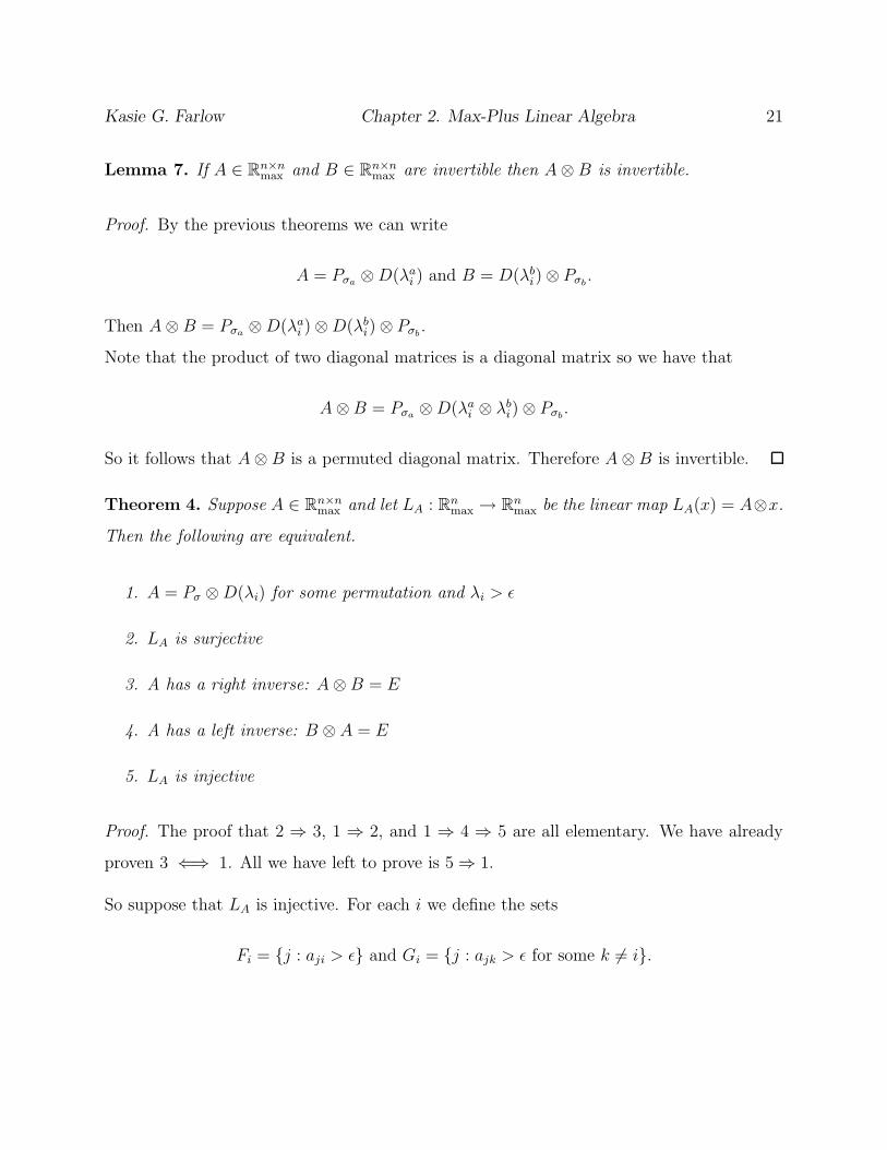
Lemma 7. If A ∈ Rn×nmax and B ∈ Rn×n
max are invertible then A⊗ B is invertible.
Proof. By the previous theorems we can write
A = Pσa ⊗D(λai ) and B = D(λb
i) ⊗ Pσb.
Then A⊗ B = Pσa ⊗D(λai ) ⊗D(λb
i) ⊗ Pσb.
Note that the product of two diagonal matrices is a diagonal matrix so we have that
A⊗B = Pσa ⊗D(λai ⊗ λb
i) ⊗ Pσb.
So it follows that A⊗ B is a permuted diagonal matrix. Therefore A⊗B is invertible.
Theorem 4. Suppose A ∈ Rn×nmax and let LA : Rn
max → Rnmax be the linear map LA(x) = A⊗x.
Then the following are equivalent.
1. A = Pσ ⊗D(λi) for some permutation and λi > ε
2. LA is surjective
3. A has a right inverse: A⊗ B = E
4. A has a left inverse: B ⊗ A = E
5. LA is injective
Proof. The proof that 2 ⇒ 3, 1 ⇒ 2, and 1 ⇒ 4 ⇒ 5 are all elementary. We have already
proven 3 ⇐⇒ 1. All we have left to prove is 5 ⇒ 1.
So suppose that LA is injective. For each i we define the sets
Fi = {j : aji > ε} and Gi = {j : ajk > ε for some k 6= i}.
Kasie G. Farlow Chapter 2. Max-Plus Linear Algebra 22
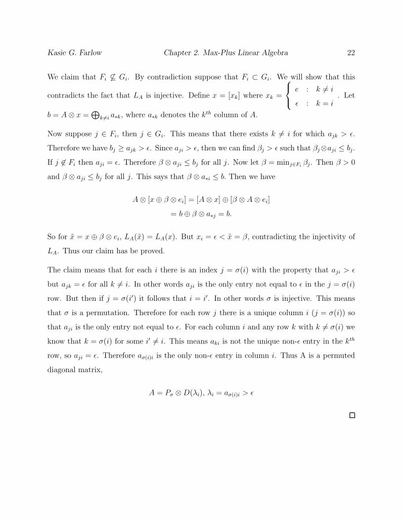
We claim that Fi 6⊆ Gi. By contradiction suppose that Fi ⊂ Gi. We will show that this
contradicts the fact that LA is injective. Define x = [xk] where xk =
e : k 6= i
ε : k = i. Let
b = A⊗ x =⊕
k 6=i a∗k, where a∗k denotes the kth column of A.
Now suppose j ∈ Fi, then j ∈ Gi. This means that there exists k 6= i for which ajk > ε.
Therefore we have bj ≥ ajk > ε. Since aji > ε, then we can find βj > ε such that βj⊗aji ≤ bj.
If j 6∈ Fi then aji = ε. Therefore β ⊗ aji ≤ bj for all j. Now let β = minj∈Fiβj. Then β > 0
and β ⊗ aji ≤ bj for all j. This says that β ⊗ a∗i ≤ b. Then we have
A⊗ [x⊕ β ⊗ ei] = [A⊗ x] ⊕ [β ⊗ A⊗ ei]
= b⊕ β ⊗ a∗j = b.
So for x = x⊕ β ⊗ ei, LA(x) = LA(x). But xi = ε < x = β, contradicting the injectivity of
LA. Thus our claim has be proved.
The claim means that for each i there is an index j = σ(i) with the property that aji > ε
but ajk = ε for all k 6= i. In other words aji is the only entry not equal to ε in the j = σ(i)
row. But then if j = σ(i′) it follows that i = i′. In other words σ is injective. This means
that σ is a permutation. Therefore for each row j there is a unique column i (j = σ(i)) so
that aji is the only entry not equal to ε. For each column i and any row k with k 6= σ(i) we
know that k = σ(i) for some i′ 6= i. This means aki is not the unique non-ε entry in the kth
row, so aji = ε. Therefore aσ(i)i is the only non-ε entry in column i. Thus A is a permuted
diagonal matrix,
A = Pσ ⊗D(λi), λi = aσ(i)i > ε
Kasie G. Farlow Chapter 2. Max-Plus Linear Algebra 23
2.2 Determinants
In conventional algebra we know that for A ∈ Rn×n det(A) =∑
σ∈Pnsgn(σ)
∏ni=1 aiσ(i), where
Pn denotes the set of all permutations of {1, 2...n} and sgn(σ) is the sign of the permutation
σ. In max-plus algebra the determinant has no direct analogue because of the absence of
additive inverses. Two related quantities, the permanent of A and the dominant of A, which
are defined below, partially take over the role of the determinant. The permanent of A is
defined similarly to the determinant but with the sgn(σ) simply omitted[25]. The following
definitions of the permanent and dominant are from [25].
Definition 20. For a matrix A ∈ Rn×nmax the permanent of A is defined to be perm(A) =
⊕
σ∈Pn
⊗ni=1(aiσ(i)), with σ and Pn is the set of all permutations of {1, 2, ...n}.
Lemma 8. If A ∈ Rn×nmax is invertible, then perm(A) 6= ε.
Proof. In max-plus algebra an invertible matrix is a diagonal matrix times a permutation
matrix. So if A is invertible the perm(A) is just the max-plus product of the diagonal entries
of the diagonal matrix. Therefore if A is invertible perm(A) 6= ε.
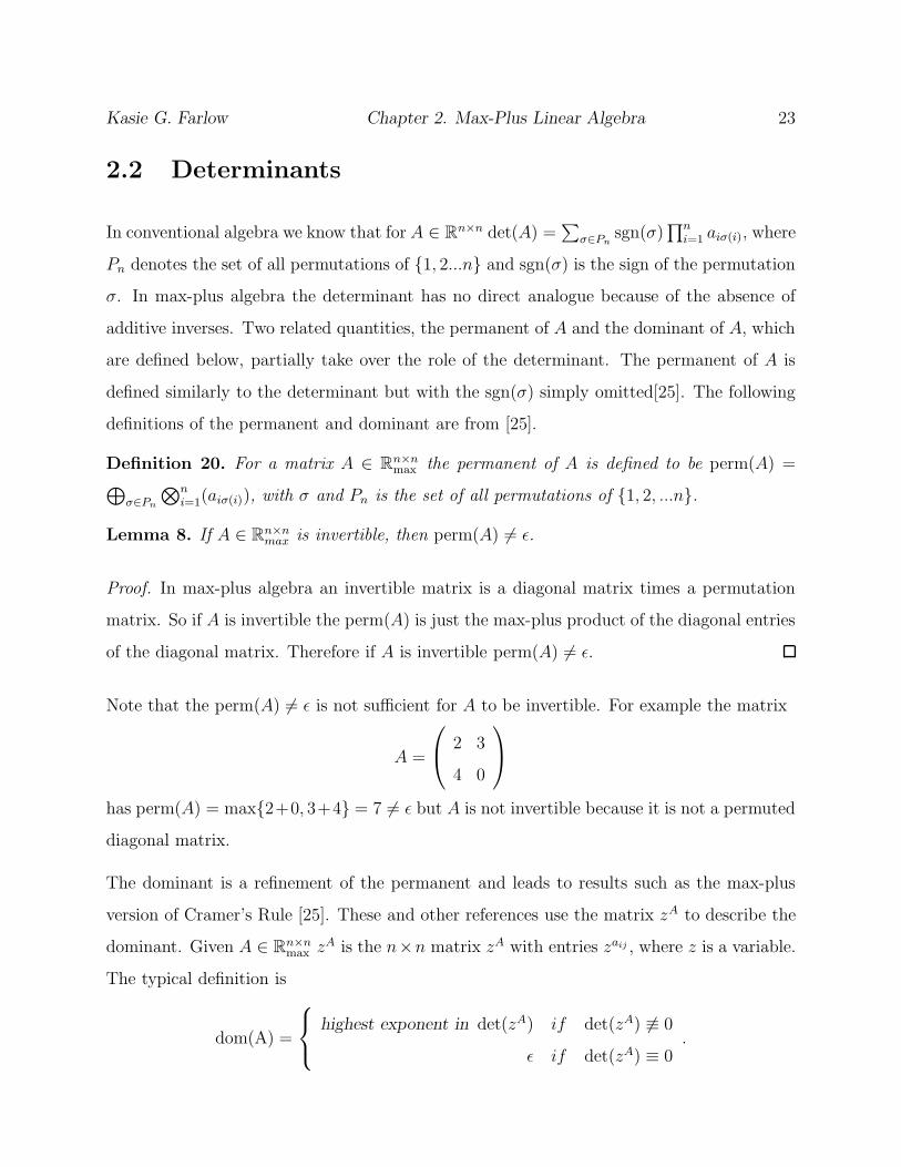
Note that the perm(A) 6= ε is not sufficient for A to be invertible. For example the matrix
A =
2 3
4 0
has perm(A) = max{2+0, 3+4} = 7 6= ε but A is not invertible because it is not a permuted
diagonal matrix.
The dominant is a refinement of the permanent and leads to results such as the max-plus
version of Cramer’s Rule [25]. These and other references use the matrix zA to describe the
dominant. Given A ∈ Rn×nmax z
A is the n×n matrix zA with entries zaij , where z is a variable.
The typical definition is
dom(A) =
highest exponent in det(zA) if det(zA) 6≡ 0
ε if det(zA) ≡ 0.

Kasie G. Farlow Chapter 2. Max-Plus Linear Algebra 24
In light of Lemma 1, we replace z by es, leading to the following two definition.
Definition 21. Given a matrix A ∈ Rn×nmax the matrix esA has entries esaij where aij ∈ Rmax
are the entries in A.
Note that this does not refer to the matrix exponential. There is no analogue of the matrix
exponential in this thesis. Here [esA]ij = esaij .
Definition 22. dom(A) =
lims→∞
1sln | det(esA)| if det(esA) 6≡ 0
ε if det(esA) ≡ 0
In terms of Definition 1, this says that | det(esA)| � esdom(A). This asymptotic connection
with the conventional determinants provides the basic approach to generalizing Cramer’s
Rule and the Cayley- Hamilton Theorem. (Note that a similar connection holds for perma-
nent : perm(esA) � esperm(A)).
Since perm(A) is the maximum diagonal value for all permutations of the columns of A, we
have the following lemma [25].
Lemma 9. dom(A) ≤ perm(A)
By the diagonal value we mean⊗n
i aiσ(i) for some σ ∈ Pn. This is true since when calculating
the dominant we can have cancellations which will not occur when calculating the permanent.
Note that due to the cancellations the dom(A) can be ε. In order for it to be possible to
have perm(A) = ε each column of A must have at least one entry equal to ε. For example
take the matrix
A =
7 4
5 2
.
We can see that dom(A) = ε since det(esA) = es9 − es9 = 0. But perm(A) = 9 ⊕ 9 = 9.
Lemma 10. If A ∈ Rn×nmax is invertible, then dom(A) 6= ε
Kasie G. Farlow Chapter 2. Max-Plus Linear Algebra 25
Proof. Since A is invertible A is a permuted diagonal matrix. Therefore the dom(A) is
equal to the max-plus product of the diagonal entries of the diagonal matrix. Therefore
dom(A) 6= ε.
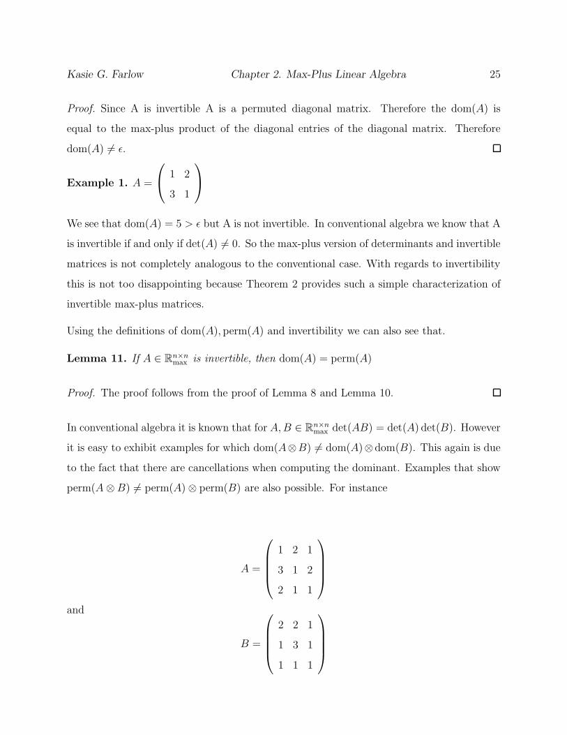
Example 1. A =
1 2
3 1
We see that dom(A) = 5 > ε but A is not invertible. In conventional algebra we know that A
is invertible if and only if det(A) 6= 0. So the max-plus version of determinants and invertible
matrices is not completely analogous to the conventional case. With regards to invertibility
this is not too disappointing because Theorem 2 provides such a simple characterization of
invertible max-plus matrices.
Using the definitions of dom(A), perm(A) and invertibility we can also see that.
Lemma 11. If A ∈ Rn×nmax is invertible, then dom(A) = perm(A)
Proof. The proof follows from the proof of Lemma 8 and Lemma 10.
In conventional algebra it is known that for A,B ∈ Rn×nmax det(AB) = det(A) det(B). However
it is easy to exhibit examples for which dom(A⊗B) 6= dom(A)⊗dom(B). This again is due
to the fact that there are cancellations when computing the dominant. Examples that show
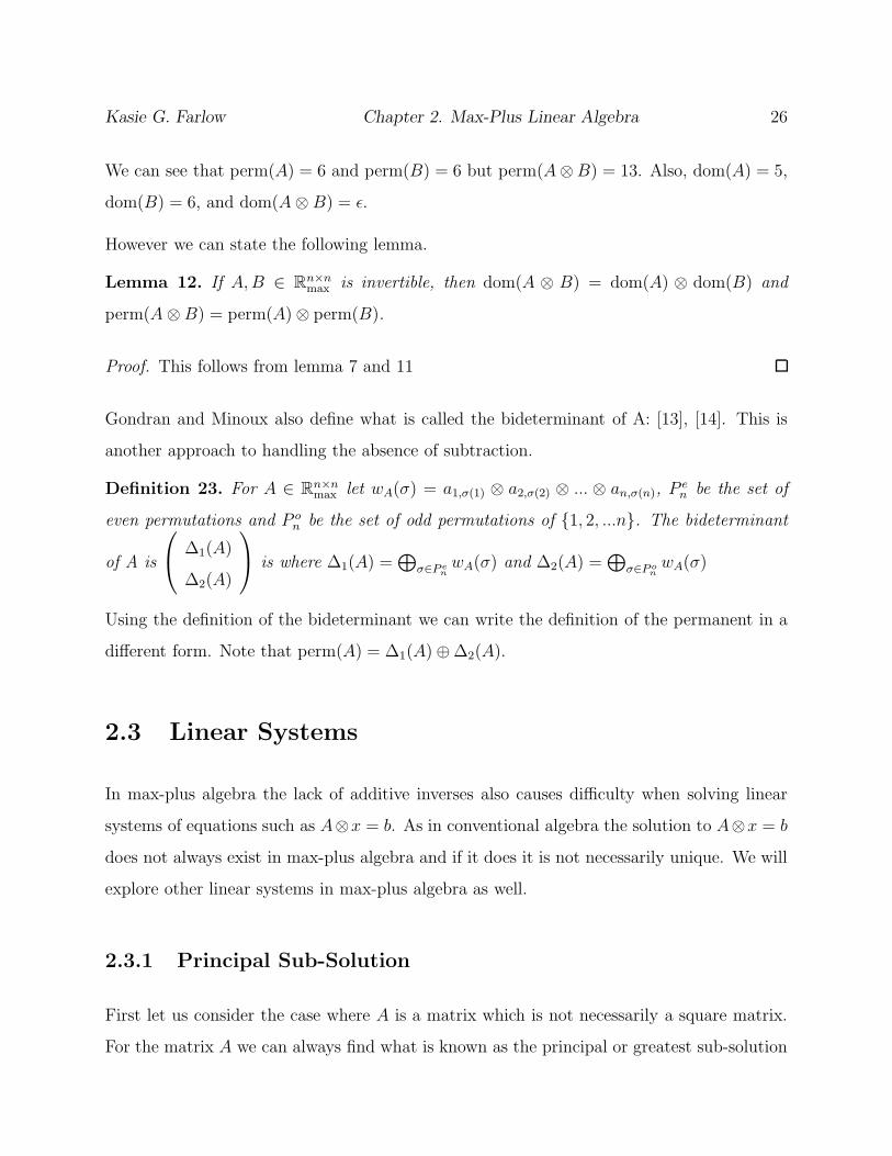
perm(A⊗B) 6= perm(A) ⊗ perm(B) are also possible. For instance
A =
1 2 1
3 1 2
2 1 1
and
B =
2 2 1
1 3 1
1 1 1
Kasie G. Farlow Chapter 2. Max-Plus Linear Algebra 26
We can see that perm(A) = 6 and perm(B) = 6 but perm(A⊗B) = 13. Also, dom(A) = 5,
dom(B) = 6, and dom(A⊗ B) = ε.
However we can state the following lemma.
Lemma 12. If A,B ∈ Rn×nmax is invertible, then dom(A ⊗ B) = dom(A) ⊗ dom(B) and
perm(A⊗B) = perm(A) ⊗ perm(B).
Proof. This follows from lemma 7 and 11
Gondran and Minoux also define what is called the bideterminant of A: [13], [14]. This is
another approach to handling the absence of subtraction.
Definition 23. For A ∈ Rn×nmax let wA(σ) = a1,σ(1) ⊗ a2,σ(2) ⊗ ... ⊗ an,σ(n), P
en be the set of
even permutations and P on be the set of odd permutations of {1, 2, ...n}. The bideterminant
of A is
∆1(A)
∆2(A)
is where ∆1(A) =⊕
σ∈P enwA(σ) and ∆2(A) =
⊕
σ∈P onwA(σ)
Using the definition of the bideterminant we can write the definition of the permanent in a
different form. Note that perm(A) = ∆1(A) ⊕ ∆2(A).
2.3 Linear Systems
In max-plus algebra the lack of additive inverses also causes difficulty when solving linear
systems of equations such as A⊗x = b. As in conventional algebra the solution to A⊗x = b
does not always exist in max-plus algebra and if it does it is not necessarily unique. We will
explore other linear systems in max-plus algebra as well.
2.3.1 Principal Sub-Solution
First let us consider the case where A is a matrix which is not necessarily a square matrix.
For the matrix A we can always find what is known as the principal or greatest sub-solution
Kasie G. Farlow Chapter 2. Max-Plus Linear Algebra 27
to A⊗ x = b The principal sub-solution is the vector largest vector x such that A ⊗ x ≤ b.
This sub-solution will be denoted by x∗(A, b). The principle sub-solution is not necessarily
a solution of A⊗ x = b. The following theorem is found in [9],[16] and [3].
Theorem 5. Let A ∈ Rm×nmax is an irreducible matrix and b ∈ Rm
max. Then [x∗(A, b)]j =
min{bi − aij : i ∈ {1, 2, ...m}and aij > ε}.
Proof. First observe that A⊗ x ≤ b is equivalent to each of the following:
1. for all i and j, aij + xj ≤ bi
2. for all i and j, xj ≤ bi − aij or aij = ε
3. for all j, xj ≤ min{bi − aij : i ∈ {1, 2....m}and aij > ε}.
This tells us that x is a solution to A⊗x ≤ b if and only if xj ≤ min{bi −aij : i ∈ {1, 2...m}}
for all j. So x∗(A,B)j = min{bi − aij : i ∈ {1, 2...m}and aij > ε} for all j is the maximum
solution of A⊗ x ≤ b.
Lemma 13. If a solution of A⊗ x = b exists, then the principle sub-solution is a solution.
Proof. let x′ be the maximum solution of A⊗ x = b then x satisfies the equation A⊗ x ≤ b.
So x′ must be the principle sub-solution. Like wise the principle sub-solution x∗(A, b) is the
maximum solution of A ⊗ x ≤ b. Which means x∗(A, b) must be the maximum solution
of A ⊗ x = b since we know a solution exists. Therefore the principle sub-solution is a
solution.
The following examples illustrate the above lemma.

Kasie G. Farlow Chapter 2. Max-Plus Linear Algebra 28
1. Let A =
2 0
1 3
, b=
5
4
. Using the previous theorem we see that the principle
solution is x =
3
1
. We find that it is in fact a solution to A⊗ x = b.
2. Let A =
3 2
1 4
, b=
20
4
. The principle solution is x =
3
0
. In this case
A⊗ x 6= b so there are no solutions.
Going back to our train example in the introduction, suppose that A is the matrix of travel
times in the train network between stations and suppose that b is the vector containing
the planned departure times of the trains for each station. Then x∗(A, b) gives the latest
departure times of the trains from the previous station such that the times contained in b
still can be met [16].
2.3.2 Cramer’s Rule
In conventional matrix algebra, when A is a non-singular matrix, Cramer’s Rule yields a
solution to the linear equation Ax = b. The solution is given by:
xi = det(a∗1,...a∗i−1,b,a∗i+1,...a∗n)det(A)
, i = 1, 2, ...n,
where a∗j denotes the jth column of A and 1 ≤ j ≤ n.
The max-plus analog to this formula developed in [25] is :
xi ⊗ dom(A) = dom(a∗1, ...a∗i−1, b, a∗i+1....a∗n).
Note that (a∗1, ...a∗i−1, b, a∗i+1, ...a∗n) is the matrix A with its ith column replaced by the
vector b. Unlike the conventional case, however, dom(A) > ε is not sufficient for this formula
to produce a solution. An additional condition is needed. The extra condition is that
Kasie G. Farlow Chapter 2. Max-Plus Linear Algebra 29
sign(a∗1, ...a∗i−1, b, a∗i+1, ....a∗n) = sign(A) for all 1 ≤ i ≤ n. Intuitively sign(A) is the sign of
the coefficient in det(esA) that contributes to the dom(A). To define sign(A) more precisely
let Pn be the set of permutations σ : {1, 2, ...n} → {1, 2, ..., n} and let t1, t2, ....tL be all
possible values such that ti =⊗n
1 (aiσ(i)) for some σ ∈ Pn.
Definition 24. Let
Si = {σ ∈ Pn : ti =⊗n
1 (aiσ(i)) for some σ ∈ Pn}
Sie = {σ ∈ Si : σ ∈ P en}
Sio = {σ ∈ Si : σ ∈ P on}
kie = |Sie| and kio = |Sio|
Then we say sign(A) = 1 if kie − kio ≥ 0 and sign(A) = −1 if kie − kio ≤ 0. If dom(A) = ε
then sign(A) = ε.
Using the above definition we can write, det(esA) =∑L
i=1(kie − kio)esti. Observe that if
sign(A) 6= ε, then sign(A) det(esA) > 0 for all sufficiently large s.
Theorem 6. If sign(a∗1, ....a∗i−1, b, a∗i+1, ....a∗n) = sign(A) for all i and dom(A) > ε then
xi ⊗ dom(A) = dom(a∗1, ...a∗i−1, b, a∗i+1....a∗n) (2.1)
yields a solution to A⊗ x = b.
Proof. Assume that dom(A) > ε and sign(a∗1, ...a∗i−1, b, a∗i+1, ...a∗n) = sign(A). We consider
the equation
esAζ = esb.
Since dom(A) > ε then det(esA) 6≡ 0 so we can use Cramer’s Rule to solve the equation
above. Cramer’s Rule yields the following:
ζi(s) = det(esa∗i ,...esa∗i−1 ,esb,esa∗i+1 ,...esa∗n)det(esA)
, 1 ≤ i ≤ n.
Kasie G. Farlow Chapter 2. Max-Plus Linear Algebra 30
Because of the hypothesis on the signs, ζi(s) > 0 for all sufficiently large s. Using Lemma 1
we see that
lims→∞
1sln ζi = (di − dom(A)), 1 ≤ i ≤ n
where di = dom(a∗1, ...a∗i−1, b, a∗i+1, ...a∗n).
The value xi = di − dom(A) are the unique solutions of (2.1). So what we have shown is
that ζi(s) � esxi. By substitution into esAζ(s) = esb we have
esb = esAζ(s) � esAesx � es(A⊗x).
By applying Lemma 1 we have shown that A⊗ x = b.
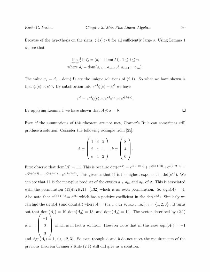
Even if the assumptions of this theorem are not met, Cramer’s Rule can sometimes still
produce a solution. Consider the following example from [25]:
A =
1 3 5
2 e 1
e 4 2
, b =
8
4
6
.
First observe that dom(A) = 11. This is because det(esA) = es(1+0+2) +es(3+1+0) +es(5+2+4)−
es(0+0+5)−es(4+1+1)−es(2+2+3). This gives us that 11 is the highest exponent in det(esA). We
can see that 11 is the max-plus product of the entries a13, a32 and a21 of A. This is associated
with the permutation (13)(32)(21)=(132) which is an even permutation. So sign(A) = 1.
Also note that es(5+2+4) = es11 which has a positive coefficient in the det(esA). Similarly we
can find the sign(Ai) and dom(Ai) where Ai = (a1, ...ai−1, b, ai+1, ...an), i = {1, 2, 3} . It turns
out that dom(A1) = 10, dom(A2) = 13, and dom(A3) = 14. The vector described by (2.1)
is x =
−1
2
3
which is in fact a solution. However note that in this case sign(A1) = −1
and sign(Ai) = 1, i ∈ {2, 3}. So even though A and b do not meet the requirements of the
previous theorem Cramer’s Rule (2.1) still did give us a solution.
Kasie G. Farlow Chapter 2. Max-Plus Linear Algebra 31
2.3.3 Solving x = (A⊗ x) ⊕ b
Now we want to consider solving the linear equation x = (A⊗ x) ⊕ b. We will see this type
of equation in Chapter 3. Under certain constraints we can solve this linear system. The
following is found in [16] and [3]. (A∗ below is the same as defined in Definition 15 on pg 16.)
Theorem 7. Let A ∈ Rn×nmax and b ∈ Rn
max. If G(A) has maximal average circuit weight less
than or equal to e, then the vector x = A∗ ⊗ b solves the equation x = (A ⊗ x) ⊕ b. If the
circuit weights of G(A) are negative then the solution is unique.
Proof. We will show that A∗ ⊗ b = A⊗ (A∗ ⊗ b)⊕ b. Using Definition 15 of A∗, and Lemma
5 on page 16 we know that since the maximal average circuit in G(A) is less then or equal
to e then A∗ exists. First observe that A∗ = A⊗ A∗ ⊕ E. Therefore we have:
A∗ ⊗ b =⊕
k≥0A⊗k ⊗ b
= (⊕
k≥1A⊗k ⊗ b) ⊕ (E ⊗ b)
= A⊗ (⊕
k≥0A⊗k ⊗ b) ⊕ (E ⊗ b)
= A⊗ (A∗ ⊗ b) ⊕ b.
This shows that x = A∗ ⊗ b is a solution. To show uniqueness we assume that all circuits
in G(A) are negative. Suppose that x is a solution of x = (A⊗ x) ⊕ b. Now substitute this
expression for x in for x on the right side. It follows that
x = b⊕ A⊗ [(A⊗ x) ⊕ b] = b⊕ (A⊗ b) ⊕ (A⊗2 ⊗ x).
By repeating this argument we see that:
x = b⊕ (A⊗ b) ⊕ (A⊗2 ⊗ b) ⊕ (A⊗3 ⊗ x)
= b⊕ (A⊗ b) ⊕ ....⊕ (A⊗(k−1) ⊗ b) ⊕ (A⊗k ⊕ x)
=⊕k−1
l=0 (A⊗l ⊗ b) ⊕ (A⊗k ⊗ x).
Using Lemma 6,Definition 15 and letting k → ∞ we get that:

Kasie G. Farlow Chapter 2. Max-Plus Linear Algebra 32
limk→∞
⊕k−1l=0 (A⊗l ⊗ b) ⊕ (A⊗k ⊗ x)
= limk→∞
⊕k−1l=0 (A⊗l ⊗ b) ⊕ lim
k→∞(A⊗k ⊗ x)
= limk→∞
(⊕k−1
l=0 A⊗l) ⊗ b⊕ lim
k→∞(A⊗k ⊗ x)
= A∗ ⊗ b⊕ ε
So x = A∗ ⊗ b is the unique solution.
2.4 Eigenvalue and Eigenvectors
Here we will study max-plus eigenvalues and eigenvectors. The max-plus eigenvalue and
eigenvectors have a graph theoretical interpretation. The relevance of many of the theorems,
lemmas and definitions from the graph theory section will be seen here. The significance of
max-plus eigenvalues and eigenvectors will also be seen in Chapter 3. The results in this
section are from [16] and [3].
Definition 25. Let A ∈ Rn×nmax be a square matrix. If µ ∈ Rmax is a scalar, v ∈ Rn
max is a
vector that contains at least one element not equal to ε, and
A⊗ v = µ⊗ v,
then µ is called an eigenvalue of A and v is an associated eigenvector of A.
Definition 26. An eigenvector is called a finite eigenvector if it has all finite entries.
In general there can be more then one eigenvalue. The definition above also allows the
eigenvalue to be equal to ε and the eigenvector to have entries equal to ε. Consider the
following lemma.
Lemma 14. ε is an eigenvalue of A if and only if A has a column of all ε entries.
Proof. Let u be an eigenvector of A associated with eigenvalue λ = ε. Define the set
I = {i : ui > ε} then J = {i : ui = ε}. Since λ is an eigenvalue the following is true.
Kasie G. Farlow Chapter 2. Max-Plus Linear Algebra 33
• For each, j ∈ J⊕
i∈I aji ⊗ ui = ε. Then aji = ε for all j.
• For each, i ∈ I⊕
i′∈I aii′ ⊗ ui′ = ε Therefore aii′ = ε for all i.
Therefore A has a column of all ε.
As a result of the previous lemma we have the following corollary.
Corollary 1. ε is not an eigenvalue of A if A is irreducible.
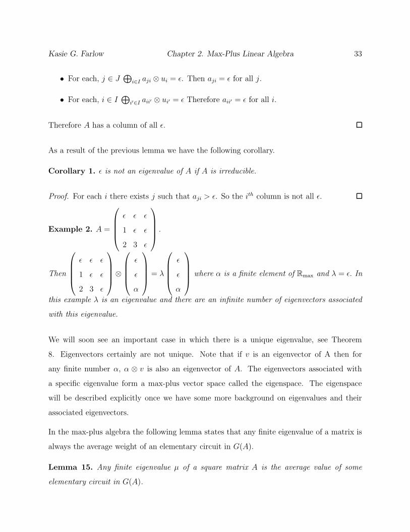
Proof. For each i there exists j such that aji > ε. So the ith column is not all ε.
Example 2. A =
ε ε ε
1 ε ε
2 3 ε
.
Then
ε ε ε
1 ε ε
2 3 ε
⊗
ε
ε
α
= λ
ε
ε
α
where α is a finite element of Rmax and λ = ε. In
this example λ is an eigenvalue and there are an infinite number of eigenvectors associated
with this eigenvalue.
We will soon see an important case in which there is a unique eigenvalue, see Theorem
8. Eigenvectors certainly are not unique. Note that if v is an eigenvector of A then for
any finite number α, α ⊗ v is also an eigenvector of A. The eigenvectors associated with
a specific eigenvalue form a max-plus vector space called the eigenspace. The eigenspace
will be described explicitly once we have some more background on eigenvalues and their
associated eigenvectors.
In the max-plus algebra the following lemma states that any finite eigenvalue of a matrix is
always the average weight of an elementary circuit in G(A).
Lemma 15. Any finite eigenvalue µ of a square matrix A is the average value of some
elementary circuit in G(A).
Kasie G. Farlow Chapter 2. Max-Plus Linear Algebra 34
Proof. By definition an associated eigenvector v of µ has at least one finite element. This
means that there exists ν1 such that vν1 6= ε. Therefore [A⊗v]ν1 = µ⊗vν1 6= ε. Hence we can
find a vertex ν2 with aν1ν2⊗vν2 = µ⊗vν1 , implying that aν1ν2 6= ε, vν2 6= ε and (ν2, ν1) ∈ E(A).
Similarly there exists ν3 such that aν2ν3 ⊗ vν3 = µ⊗ vν2 with (ν3, ν2) ∈ E(A). Continuing in
this fashion there exists a vertex νk that we will encounter twice for the first time, νk = νk+`,
since the number of vertices in finite. So we have found an elementary circuit,
c = ((νk, νk+`−1), (νk+`−1, νk+`−2), ..., (νk+1, νk)).
This has length ||c||l = ` and weight ||c||w =⊗`−1
j=0 aνk+jνk+j+1, where νk = νk+`. By con-
struction we have
⊗`−1j=0(aνk+jνk+j+1
⊗ vνk+j+1) = µ⊗` ⊗
⊗`−1j=0 vνk+j
.
Since ⊗ converts to + in conventional algebra the equation above can be written as
∑`−1j=0(aνk+jνk+j+1
+ vνk+j+1) = `µ+
∑`−1j=0 vνk+j
.
We also have that
∑`−1j=0 vνk+j+1
=∑`−1
j=0 vνk+j
since νk = νk+`. Using this fact we can subtract∑`−1
j=0 vνk+jfrom both sides giving us,
⊗`−1j=0 aνk+jνk+j+1
= `× µ.
This means that ||c||w = `× µ = µ⊗`. Then the average value of the circuit c is
||c||w||c||`
= µ⊗`
`= µ.
Lemma 16. Let C(A) denote the set of elementary circuits in G(A). Then
Kasie G. Farlow Chapter 2. Max-Plus Linear Algebra 35
maxp∈C(A)||p||w||p||l
is the maximal average circuit.
The proof follows from the fact that every circuit is made up of elementary circuits. Recall
Definition 12 of an elementary circuit.
Definition 27. A circuit p ∈ C(A) is called critical if its average weight is maximal.
Definition 28. The critical graph of A is denoted by Gc(A) and contains the vertices and
edges belonging to the critical circuits of G(A). The set of vertices in Gc(A) are denoted by
V c(A).
The vertices in Gc(A) are often called the critical vertices. We now have the following
definition from [1].
Definition 29. The critical classes of A are the strongly connected components of Gc(A)
Lemma 17. If G(A) contains at least one circuit then any circuit in Gc(A) is critical.
Proof. Let λ be the maximal average circuit of A. Without loss of generality we can assume
that λ = 0. Now suppose by contradiction that Gc(A) contains a circuit ρ with average
value not equal to zero. Since ρ is a circuit in Gc(A) then ρ is a circuit in G(A). If the
average weight of ρ is larger then zero , then the maximal average circuit weight of A is
larger then zero which contradicts the fact that λ = 0. Now consider the case when ρ is
less then zero. Note that ρ is a path made up of sub-paths ρi, a sub-path of some critical
circuit ci, i ∈ {1, 2..., k}. Therefore there exists sub-paths ζi such that ci is made up of the
two sub-paths ζi and ρi. Since all circuits ci have weight zero then the circuit made of the
sub-paths ζi is a circuit with weight greater then zero. This again contradicts the fact that
λ = 0. Therefore every circuit in Gc(A) is a critical circuit.
Definition 30. Let λ be a finite eigenvalue of A. The matrix Aλ is defined by [Aλ]ij = aij−λ
Kasie G. Farlow Chapter 2. Max-Plus Linear Algebra 36
This matrix is called the normalized matrix and will be important in the proof of Lemma 19.
Note that the eigenspace of A and Aλ coincide and e is an eigenvalue of Aλ. This is easy to
see since
[λ⊗ v]j = [A⊗ v]j if and only if vj = [A⊗ v]j − λ if and only if e⊗ vj = [Aλ ⊗ v]j.
Similarly we have the following lemma.
Lemma 18. Let A ∈ Rn×nmax be an irreducible matrix with finite eigenvalue λ, and let v be an
associated eigenvector. Then, A∗λ has eigenvalue e and v is an associated eigenvector.
Proof. It can be shown that
(E ⊕ Aλ) ⊗ v = v.
It follows from Lemma 5 that
A∗λ = (E ⊕ Aλ)
⊗(n−1).
Therefore,
A∗λ ⊗ v = (E ⊕ Aλ)
⊗(n−1) ⊗ v = v.
Lemma 19. Let the communication graph G(A) of A ∈ Rn×nmax have a finite maximal average
circuit weight λ. Then λ is an eigenvalue of A and for any ν ∈ V c(A), the column [A∗λ]ν is
an eigenvector of A associated with λ.
Proof. Let λ be the maximal average circuit of G(A). It is clear that the maximal average
circuit of G(Aλ) is e = 0. Therefore, by Lemma 5 on pg 16, A+λ is well defined. As we saw
Kasie G. Farlow Chapter 2. Max-Plus Linear Algebra 37
above the critical circuits of A and Aλ coincide. Likewise except for the weights of the edges,
the graphs Gc(A) and Gc(Aλ) coincide. Therefore
for any ν ∈ V c(A), [A+λ ]νν = e, (2.2)
since any critical circuit from ν to ν in G(A) has average weight λ.
Recalling Definition 15 and Lemma 5 on page 16, we see that
A∗λ = E ⊕ A+.
It follows that
[A∗λ]iν = [E ⊕ A+
λ ]iν =
ε⊕ [A+λ ]iν : for i 6= ν
e⊕ [A+λ ]iν : for i = ν
.
Using (2.2) this implies [A∗λ]ν = [A+
λ ]ν . It is easy to see that A+λ = Aλ ⊗ A∗
λ. So we have
that, for ν ∈ V c(A);
Aλ ⊗ [A∗λ]ν
= [Aλ ⊕ A∗λ]ν
= [A+λ ]ν
= [A∗λ]ν.
Therefore A⊗ [A∗λ]ν = λ⊗ Aλ ⊗ [A∗
λ]ν = λ⊗ [A∗λ]ν.
Thus λ is an eigenvalue of A and the νth column of A∗λ is an eigenvector of A for any
ν ∈ V c(A).
Definition 31. The columns of [A∗λ]ν for ν ∈ V c(A) are called the critical columns of A.
We have mentioned that eigenvalues and eigenvectors are not unique. However if A ∈ Rn×nmax
is an irreducible matrix then we have the following theorem
Kasie G. Farlow Chapter 2. Max-Plus Linear Algebra 38
Theorem 8. If A ∈ Rn×nmax is an irreducible matrix the maximal average circuit weight is the
unique eigenvalue.
Proof. Assume A is irreducible and λ is the maximal average circuit in G(A). If A is
irreducible then G(A) contains at least one circuit so λ must be finite where λ is a eigenvalue
by Lemma 15. Now we will show that the eigenvalue of A is unique if A is irreducible. First
pick an elementary circuit c = ((i1, i2), (i2, i3), ...(il, i`+1)) in G(A) of length ||c||l = ` and
i1 = i`+1. So aik+1ik 6= ε for k = {1, 2...`}. Let µ be the eigenvalue of A and let v be an
associated eigenvector. Since A is irreducible the µ must be finite. By assumption we have
µ⊗ v = A⊗ v so it follows that
aik+1ik ⊗ vik ≤ µ⊗ vik+1for k ∈ {1, 2...`}.
Using the same argument as lemma 15 we have that
||c||w||c||l
≤ µ⊗`
`= µ.
This holds for any circuit in C(A). So any finite eigenvalue µ has to be larger or equal to
the maximal average circuit λ. By lemma 15 we know that any finite eigenvalue is the
average value of a circuit in G(A). Therefore λ is a finite eigenvalue of A which is uniquely
determined.
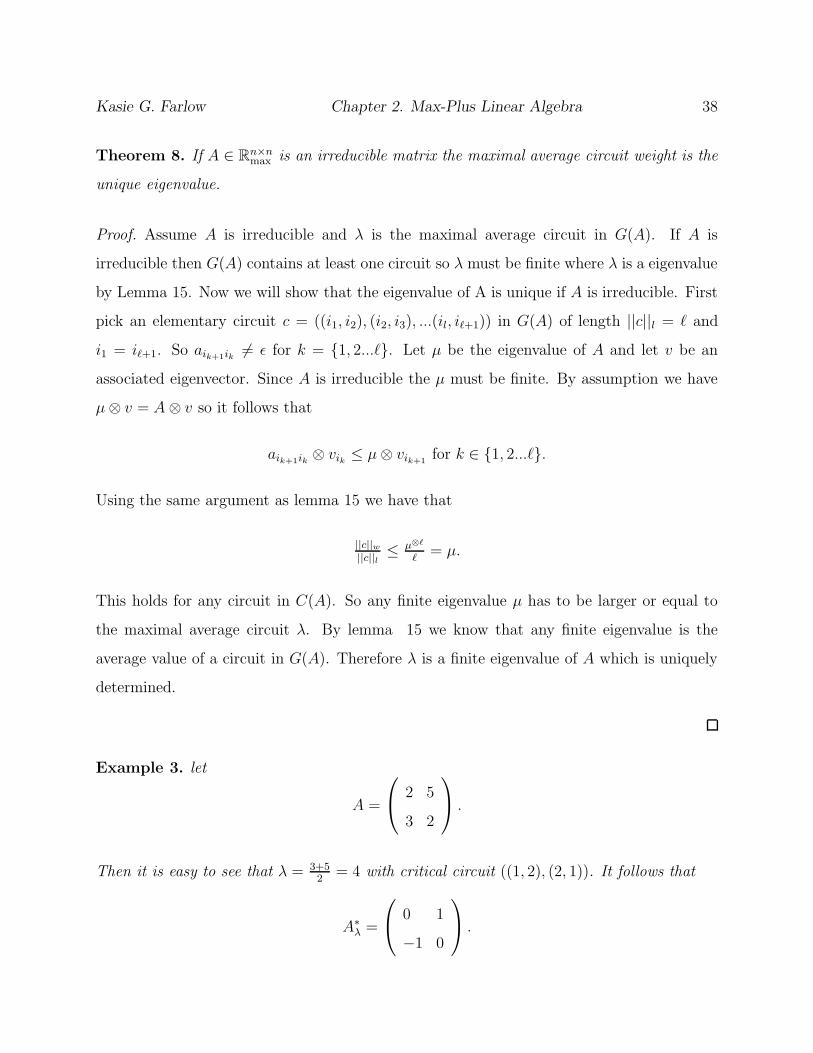
Example 3. let
A =
2 5
3 2
.
Then it is easy to see that λ = 3+52
= 4 with critical circuit ((1, 2), (2, 1)). It follows that
A∗λ =
0 1
−1 0
.
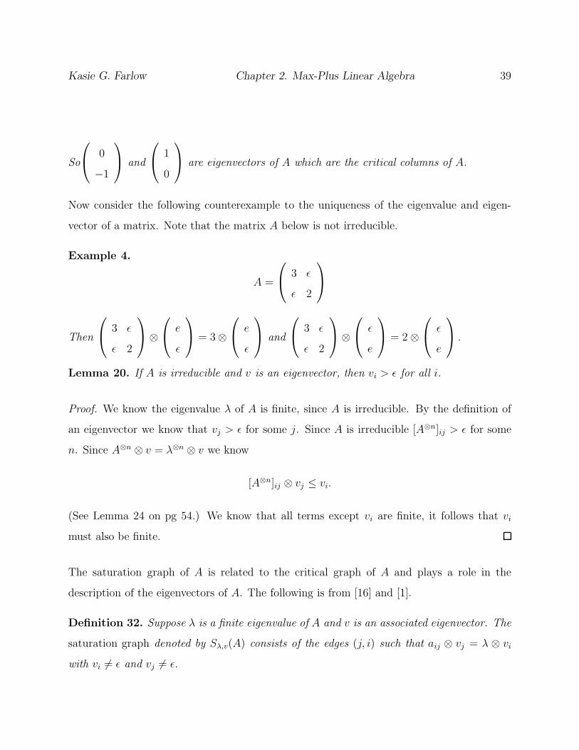
Kasie G. Farlow Chapter 2. Max-Plus Linear Algebra 39
So
0
−1
and
1
0
are eigenvectors of A which are the critical columns of A.
Now consider the following counterexample to the uniqueness of the eigenvalue and eigen-
vector of a matrix. Note that the matrix A below is not irreducible.
Example 4.
A =
3 ε
ε 2
Then
3 ε
ε 2
⊗
e
ε
= 3 ⊗
e
ε
and
3 ε
ε 2
⊗
ε
e
= 2 ⊗
ε
e
.
Lemma 20. If A is irreducible and v is an eigenvector, then vi > ε for all i.
Proof. We know the eigenvalue λ of A is finite, since A is irreducible. By the definition of
an eigenvector we know that vj > ε for some j. Since A is irreducible [A⊗n]ij > ε for some
n. Since A⊗n ⊗ v = λ⊗n ⊗ v we know
[A⊗n]ij ⊗ vj ≤ vi.
(See Lemma 24 on pg 54.) We know that all terms except vi are finite, it follows that vi
must also be finite.
The saturation graph of A is related to the critical graph of A and plays a role in the
description of the eigenvectors of A. The following is from [16] and [1].
Definition 32. Suppose λ is a finite eigenvalue of A and v is an associated eigenvector. The
saturation graph denoted by Sλ,v(A) consists of the edges (j, i) such that aij ⊗ vj = λ ⊗ vi
with vi 6= ε and vj 6= ε.
Kasie G. Farlow Chapter 2. Max-Plus Linear Algebra 40
Recall that a finite vector has all finite entries. As a result of the previous definition we have
the following lemma.
Lemma 21. Suppose A ∈ Rn×nmax with finite eigenvalue λ and associated finite eigenvector v
(1) For each vertex i ∈ Sλ,v(A) there exists a circuit in Sλ,v(A) from which i can be reached
in a finite number of steps.
(2) All circuits of Sλ,v(A) have average circuit weight λ.
(3) If A is irreducible, then circuits of Sλ,v(A) are critical.
(4) If A is irreducible, Gc(A) ⊆ Sλ,v(A) .
Proof. For (1) let i be a vertex in Sλ,v(A). Then there exists a vertex j ∈ Sλ,v(A) such
that λ ⊗ vi = aij ⊗ vj with vi, vj 6= ε. Repeating this we can find a vertex k such that
λ⊗ vj = ajk ⊗ vk with vj, vk 6= ε. We can repeat this an arbitrary number of times. Assume
we continue this m times, then we get a path of length m in Sλ,v(A). If n < m then the path
we constructed contains an elementary circuit. Thus our proof of (1) is complete.
For (2) Consider the elementary circuit c ∈ Sλ,v(A) where c = ((i1, i2), (i2, i3), ...(i`, i`+1 =
i1)). By the definition of a saturation graph we have
λ⊗ vik+1= aik+1ik ⊗ vik , 1 ≤ k ≤ l.
This implies that
λ⊗` ⊗ vi1 =⊗`
k=1 aik+1ik ⊗ vi1 .
Therefore we have λ⊗l =⊗`
k=1 aik+1ik .The expression on the right-hand side is the weight of
circuit c. Therefore c has average weight λ.
For (3) we recall that since A is irreducible it has a unique eigenvalue λ which is the maximum
average circuit weight. By part (2) we know that any circuit in the saturation graph has
Kasie G. Farlow Chapter 2. Max-Plus Linear Algebra 41
average circuit weight λ . Therefore the average circuit weight of any circuit in the saturation
graph is the maximal average circuit weight of G(A), so it belongs to the critical graph of
A.
For (4) since A is irreducible, then A has a unique finite eigenvalue λ. The irreducibility of
A also implies that vi > ε for all the entries of the eigenvector v.(See the previous lemma.)
Consider any edge (i, j) ∈ Gc(A). We want to show that
aji ⊗ vi = λ⊗ vj, (2.3)
which would imply that (i, j) ∈ Sλ,v(A). Since A ⊗ v = λ ⊗ v we know aji ⊗ vi ≤ λ ⊗ vj.
Suppose that the inequality was strict,
aji ⊗ vi < λ⊗ vj. (2.4)
Since (i, j) ∈ Gc(A) there is a critical circuit c : ((i1, i2), (i2, i3), ...(i`, i`+1 = i1)) with i1 = i
and i2 = j. Then for each k = 1, 2, ...` we have
aik+1ik ⊗ vk ≤ λ⊗ vk+1
and for the first (k = 1) the inequality is strict. Summing around the circuit gives us,
⊗`k=1 aik+1ik ⊗
⊗`k=1 vik < λ⊗` ⊗
⊗`k=1 vik+1
= λ⊗` ⊗⊗`
k=1 vik .
The inequality is strict because of (2.4). Since vi > ε it follows that
⊗`k=1 aik+1ik < λ⊗`.
But this means the average weight of out circuit c is less then λ, which is contrary to
the assumption that c is critical. Therefore aji ⊗ vi = λ ⊗ vj so (i, j) ∈ Sλv(A). Thus
Gc(A) ⊆ Sλv(A).

Kasie G. Farlow Chapter 2. Max-Plus Linear Algebra 42
As previously mentioned the eigenvectors of A form a max-plus vector space called the
eigenspace of A which is the set of all eigenvectors of A. Let A have finite eigenvalue λ. We
will denote the eigenspace of A by Vλ(A).
Theorem 9. If A is an irreducible matrix then the eigenspace of A is given by:
Vλ(A) = {v ∈ Rnmax : v =
⊕
i∈V c(A) ai ⊗ [A∗λ]i for ai ∈ Rmax}
Proof. First we know from Lemma 19 that [A∗λ]i for all i ∈ V c(A) are eigenvectors of A.
Since any max-plus linear combination of eigenvectors is an eigenvector, it follows that
⊕
i∈V c(A) ai ⊗ [A∗λ]i
is an eigenvector where ai ∈ Rmax and at least one ai 6= ε. For the converse we will show that
any eigenvector can be be written as a linear combination of the critical columns of A. Since
A has eigenvalue λ with associated eigenvector v then A∗λ has eigenvalue e and eigenvector v.
Now consider vertices i and j in the saturation graph Se,v(Aλ) such that there exists a path
from i to j. By Lemma 21, for each j there exists i that belongs to a critical circuit. Now
Let ((i1, i2), (i2, i3)..., (i`, i`+1)), with i = i1 and j = i`+1. By the definition of the saturation
graph we have
[Aλ]ik+1ik ⊗ vik = vik+1, 1 ≤ k ≤ `.
Hence
vj = α⊗ vi,
where α =⊗
k=1
[Aλ]ik+1ik ≤ [A⊗`λ ]ji ≤ [A∗
λ]ji. (2.5)
Using the fact that vj = α⊗ vi for any vertex η we have
Kasie G. Farlow Chapter 2. Max-Plus Linear Algebra 43
[A∗λ]ηj ⊗ vj = [A∗
λ]ηj ⊗ α⊗ vi
≤ [A∗λ]ηj ⊗ [A∗
λ]ji ⊗ vi ( by (2.5))
≤ [A∗λ]ηi ⊗ vi (2.6)
The last inequality follows from the fact that A∗λ ⊗ A∗
λ = A∗λ. (2.6) gives us that
⊕
j∈Se,v(Aλ)
[A∗λ]ηj ⊗ vj ≤
⊕
i∈V c(Aλ)
[A∗λ]ηi ⊗ vi. (2.7)
Since v is the eigenvector of Aλ associated with eigenvalue e, we know v = A∗λ ⊗ v. This
means that vη = [A∗λ]ηj ⊗ vj for some j in the saturation graph. We don’t know which j but
since j is in the saturation graph it holds that
vη =⊕
j∈Se,v(Aλ)[A∗λ]ηj ⊗ vj ≤
⊕
i∈V c(Aλ)[A∗λ]ηi ⊗ vi (by (2.7)).
Therefore
vη ≤⊗
i∈V c(Aλ)[A∗λ]ηi ⊗ vi.
Conversely since v is an eigenvector of A∗λ for eigenvalue e,
vη = [A∗λ ⊗ v]η =
⊕nj=1[A
∗λ]ηj ⊗ vj ≥
⊕
i∈V c(Aλ)[A∗λ]ηi ⊗ vi.
Hence vη =⊕
i∈V c(Aλ)[A∗λ]ηi ⊗ vi.
Lemma 22. Let A be an irreducible matrix. For vertices i and j which belong to the critical
graph of A, there exists a ∈ R such that
a⊗ [A∗λ]∗i = [A∗
λ]∗j
if and only if i and j belong to the same critical class.
Kasie G. Farlow Chapter 2. Max-Plus Linear Algebra 44
In other words all columns from the same critical class are scalar multiples of each other.
Proof. First assume that i and j belong to the same critical class of Aλ (recall that the
critical classes of A and Aλ coincide). It follows that [A∗λ]ji ⊗ [A∗
λ]ij = e. Therefore for all `,
[A∗λ]`i ⊗ [A∗
λ]ij ≤ [A∗λ]`j
= [A∗λ]`j ⊗ [A∗
λ]ji ⊗ [A∗λ]ij (since[A∗
λ]ji ⊗ [A∗λ]ij = e)
≤ [A∗λ]`i ⊗ [A∗
λ]ij.
Which tells us that
[A∗λ]`i ⊗ [A∗
λ]ij ≤ [A∗λ]`j ≤ [A∗
λ]`i ⊗ [A∗λ]ij,
so [A∗λ]`i ⊗ [A∗
λ]ij = [A∗λ]`j. By letting a = [A∗
λ]ij we have shown that a⊗ [A∗λ]∗i = [A∗
λ]∗j .
Now we want to show that if i and j do not belong to the same critical class then a⊗ [A∗λ]∗i =
[A∗λ]∗j does not hold. So suppose that i and j do not belong to the same critical class but
that a⊗ [A∗λ]∗i = [A∗
λ]∗j . It follows that
a⊗ e = [A∗λ]ij and a⊗ [A∗
λ]ji = e
so that [A∗λ]ji ⊗ [A∗
λ]ij = e. Therefore the circuits formed by the edges (i, j) and (j, i) have
average weight e where i and j belong to the critical graph of A. So they belong to the same
critical class which is a contradiction.
In general the eigenvectors of A ∈ Rn×nmax are not unique. However we will consider a situation
when the eigenvectors are unique (up to scalar multiples).
Definition 33. For A ∈ Rn×nmax the eigenvector of A is unique if for any two eigenvectors
v, w ∈ Rnmax v = α⊗ w for some α ∈ R
As result of the previous lemma we have:
Kasie G. Farlow Chapter 2. Max-Plus Linear Algebra 45
Lemma 23. If A ∈ Rn×nmax is irreducible the A has a unique critical class if and only if the
eigenvector of A is unique.
Proof. First assume A has a unique critical class. By Lemma 22 we know if i and j belong
to the same critical class then a ⊗ [A∗λ]∗i = [A∗
λ]∗j . So since A has only one critical class
then the eigenvector is unique. For the other direction if v is a unique eigenvector then
a⊗ [A∗λ]∗i = [A∗
λ]∗j for all critical vertices. By the previous theorem these vertices belong to
the same critical class. Hence A has a unique critical class.
There are several algorithms for computing the eigenvalue of an irreducible matrix such as
Karp’s algorithm and the power algorithm; see [16] and [5]. These algorithms will not be
described here.
For reducible matrices the eigenvalue and eigenvectors of A are not necessarily finite and the
eigenvalue may not be unique. Thus the eigenspace is much more complicated than in the
irreducible case. We will not discuss the case when A is reducible here. See [16] for more
discussion on this matter.
2.5 Cayley-Hamilton and the Max-Plus Characteristic
Equation
Recall that in conventional linear algebra the Cayley-Hamilton Theorem states that every
square matrix A satisfies its own characteristic equation. The characteristic equation in
conventional algebra is used to solve for the eigenvalue of a matrix. We begin with the
following theorem which is the conventional version of the Cayley-Hamilton Theorem. Let
Ckn be the set of all subsets of k elements of the set {1, 2, ..., n}. If A is a n× n matrix and
ϕ ⊂ {1, 2...n}, the submatrix obtained by removing all rows and columns of A except those
denoted by ϕ is denoted by Aϕϕ.

Kasie G. Farlow Chapter 2. Max-Plus Linear Algebra 46
Theorem 10. Suppose A ∈ Rn×n, if
det(λI − A) = λn + c1λn−1 + ...+ cn−1λ+ cn then
An + c1An−1 + ... + cn−1A+ cnI = 0
where the ck are given by ck = (−1)k∑
σ∈Ckndet(Aσσ).
We will show how the Cayley- Hamilton Theorem can be translated into max-plus algebra.
These results are found in [25] and [6]. Again we consider the matrix esA. We also need a
few more definitions. First we have that the characteristic polynomial of the matrix- valued
function esA is given by:
det(λI − esA) = λn + γ1(s)λn−1 + ...+ γn−1(s)λ+ γn(s) (2.8)
with coefficients
γk(s) = (−1)k∑
ϕ∈Ckndet(esAϕϕ).
Therefore
(esA)n + γ1(s)(esA)n−1 + ... + γn−1(s)e
sA + γnI = 0. (2.9)
This is just the result of applying Theorem 10 to the matrix esA. Next recall that Pn
represents the set of permutations σ : {1, 2, ...n} → {1, 2, ..., n} where P en represents the even
permutations and P on represents the odd permutations.
Now we define Γk = {ζ : ∃{i1, i2, ..., ik} ∈ Ckn, ∃ρ ∈ Pk such that ζ =
∑kr=1 airiρ(r)} for
k = 1, 2, ...n. These values are the values ζ for which esζ occurs in γk(s). To describe the
coefficients of esζ in γk(s) we define the following. For every k ∈ {1, 2, ...n} and for every
ζ ∈ Γk we define the values:
Iek(ζ) is the number of ρ ∈ P e
k such that there exists {i1, i2, ...ik} ∈ Ckn and ζ =
∑kr airiρ(r)
Iok(ζ) is the number of ρ ∈ P o
k such that there exists {i1, i2, ...ik} ∈ Ckn and ζ =
∑kr airiρ(r)
.
Kasie G. Farlow Chapter 2. Max-Plus Linear Algebra 47
Then Ik(ζ) = Iek(ζ) − Io
k(ζ).
Now we can write
γk(s) = (−1)k∑
ζ∈Γk
Ik(s)esζ . (2.10)
The dominant term in γk(s) is given by edk where
dk = max{ζ ∈ Γk : Ik(ζ) 6= 0}.
Applying Lemma 1 to (2.10) we have
|γk(s)| � esdk .
Now define the leading coefficients of γk(s): γk = (−1)kI(dk) for k = 1, 2...n. In brief
γk(s) = γkesdk + (lower order terms). We need to separate the terms (k) with positive γk
from those with negative γk. Let ` = {k : γk > 0} and = {k : γk < 0}. For every
ζ ∈ Γ1 = {aii : i = 1, 2, ...n}, we have that Io1(ζ) = 0 and Ie
1(ζ) > 0. This implies that
I1(d1) > 0 and that γ1 < 0. Therefore we always have 1 ∈ .
The max-plus characteristic equation of A is also found by rearranging (2.8) and moving the
γk(s)λn−k for which γk(s) has a negative leading coefficient to the right side, replace λ with
esλ, and then applying Lemma 1. The reason for doing this is that subtraction is not defined
in the max-plus algebra. We state this in the following definition.
Definition 34. The max-plus characteristic equation of A ∈ Rn×nmax is defined as
λ⊗n ⊕⊕
k∈`
dk ⊗ λ⊗n−k =⊕
k∈
dk ⊗ λ⊗n−k (2.11)
Now we can state and prove the following theorem
Theorem 11. A ∈ Rn×nmax . The A satisfies its own characteristic equation:
A⊗n ⊕⊕
k∈`
dk ⊗ A⊗n−k =⊕
k∈
dk ⊗ A⊗n−k. (2.12)
Kasie G. Farlow Chapter 2. Max-Plus Linear Algebra 48
Proof. We continue with the application of the conventional Cayley-Hamilton Theorem to
the matrix esA. If A ∈ Rn×nmax then it is easy to see that
(esA)k � esA⊗k
.
Now since γk(s) � γkesdk so after rearrangement (2.9) becomes
esA⊗n
+∑
k∈`
γk(s)esdkesA⊗n−k
� −∑
k∈
γk(s)esdkeA⊗n−k
. (2.13)
Using Lemma 1 we get the following expression in Rmax,
A⊗n ⊕⊕
k∈`
dk ⊗ A⊗n−k =⊕
k∈
dk ⊗ A⊗n−k. (2.14)
Let us now consider an example from [6].
Example 5. Let
A =
−2 1 ε
1 0 1
ε 0 2
.
Using the definitions above we find that Γ1 = {2, 0,−2}, Γ2 = {2, 1, 0,−2, ε} and Γ3 =
{4, 0,−1, ε}. Now we see that
I1(2) = 1, I1(0) = 1, I1(−2) = 1
I2(2) = 0, I2(1) = −1, I2(0) = 1, I2(−2) = 1, I2(ε) = −1
I3(4) = −1, I3(0) = 1, I3(−1) = −1, I3(ε) = 1.
Hence d1 = 2, d2 = 1 and d3 = 4. Note that the maximum value in Γ2 is 2 however
I2(2) = 0 So an even and an odd permutation gives us the diagonal value 2 which means the
Kasie G. Farlow Chapter 2. Max-Plus Linear Algebra 49
two permutations cancel each other out so d2 = 1. γ1 = −1, γ2 = −1 and γ3 = 1 so ` = 3
and = {1, 2}. Therefore the max-plus characteristic equation of A is
λ⊗3 ⊕ 4 = 2 ⊗ λ⊗2 ⊕ 1 ⊗ λ (2.15)
and A satisfies its max plus characteristic equation with
A⊗3 ⊕ 4 ⊗ E = 2 ⊗ A⊗2 ⊕ 1 ⊗ A =
4 3 4
3 4 5
3 4 6
. (2.16)
In [25] Olsder and Roos described the max-plus characteristic equation, but had a subtle
flaw. De Schutter and De Moor [6] found a counterexample, and were able to fix Olsder and
Roos’s mistake. The correction will be summarized here. In [25] Olsder and Roos claimed
that the highest exponential factor in γk(s) is equal to the max{dom(Aσσ) : σ ∈ Ckn} rather
than dk and that
γk(s) = (−1)kγkes max{dom(Aσσ):σ∈Ck
n}.
However this is not necessarily true because the even and odd permutations may cancel,
eliminating that exponential factor. Our example A above is the counterexample cited by
De Schutter and De Moor. Consider γk(s). First we have that
det(esA{1,2}{1,2}) = es(−2) − es2
det(esA{1,3}{1,3}) = es0 − es(−∞) = 1
det(esA{2,3}{2,3}) = es2 − es1.
dom(A{1,2}{1,2}) = 2, dom(A{1,3}{1,3}) = 0 and dom(A{2,3}{2,3}) = 2 , so max{dom(Aσσ) : σ ∈
C23} = 2. However,
γ2(s) = (−1)2(det(esA{1,2}{1,2}) + det(esA{1,3}{1,3}) + det(esA{2,3}{2,3}))
= es(−2) − es2 + es0 − es(−∞) + es2 − es1
= es(−2) + es0 − es(−∞) − es1
Kasie G. Farlow Chapter 2. Max-Plus Linear Algebra 50
and the highest degree in γ2(s) is 1.
Now consider the following theorem.
Theorem 12. The eigenvalues of A ∈ Rn×nmax satisfy the characteristic equation of A
Proof. Suppose v is an eigenvalue associated with the eigenvalue λ of A. Now consider (2.14).
We can multiply v on both sides of that equation giving us
λ⊗n ⊗ v ⊕⊕
k∈` dk ⊗ λ⊗n−k ⊗ v =⊕
k∈ dk ⊗ λ⊗n−k ⊗ v.
(See Lemma 24 on pg 54.) Now we can subtract (in the conventional sense) v from both
sides of the equation which gives us
λ⊗n ⊕⊕
k∈` dk ⊗ λ⊗n−k =⊕
k∈ dk ⊗ λ⊗n−k.
Thus our proof is complete.
If ρ is a root of the characteristic equation of A then ρ is not necessarily an eigenvalue of A.
To see this consider the matrix
A =
2 7
−3 4
.
Using the formulas we have defined for the max-plus characteristic equation of A we see
that:
Γ1 = {2, 4} and Γ2 = {6, 4} with I1(2) = 1 , I1(4) = 1, I2(6) = 1 and I2(4) = −1.
Therefore d1 = 4, d2 = 6, γ1 = −1 and γ2 = 1 with ` = {2} and = {1}. So the characteristic
equation is λ⊗2 ⊕ 6 = 4 ⊗ λ. We observe that both 2 and 4 are roots of the characteristic
equation but since A is irreducible it has a unique eigenvalue given by the maximal average
circuit weight, which turns out to be 4. Thus ρ = 2 satisfies the characteristic equation of A
but is not an eigenvalue of A.

Kasie G. Farlow Chapter 2. Max-Plus Linear Algebra 51
2.6 Linear Dependence and Independence
As in conventional linear algebra we can define the linear dependence and independence
of vectors in the max-plus sense. However the definitions are a little more complex. The
following can be found in [12], [13], [3] and [2].
Recall that the max-plus algebra is an idempotent semi-ring. In order to define linear
dependence, independence and bases we need the definition of a semi-module. A semi-
module is essentially a linear space over a semi-ring. Semimodules and subsemimodules are
analogous to modules and submodules over rings [2].
Definition 35. A set V ⊂ Rnmax is a commutative idempotent semi-module over Rmax if it
is closed under ⊕ and scalar multiplication; α⊗ v ∈ V and u⊕ v ∈ V for all α ∈ Rmax and
u, v ∈ Rnmax.
Definition 36. A finitely generated semi-module V ⊂ Rnmax is the set of all linear combina-
tions of a finite set {u1, u2, ...ur} of vectors in Rnmax:
V = {⊕r
i=1 αi ⊗ ui|α1, α2, ...αr ∈ Rmax}.
Definition 37. A element x can be written as a finite linear combination of elements of
F ⊆ V if x =⊕
f∈F λf ⊗ f , for some λf ∈ Rmax such that λf = ε for all but finitely many
f ∈ F .
As noted above linear independence and dependence in the max-plus sense are not com-
pletely analogous to the conventional definition. There are different interpretations of linear
independence, dependence and bases. We will consider the definitions of linear dependence
and linear independence due to Gondran and Minoux [13].
Definition 38. A set of p vectors {v1, v2, ...vp} ∈ Rnmax is linearly dependent if the set
{1, 2, ...p} can be partitioned into disjoint subsets I and K such that for j ∈ I ∪K there exist
αj ∈ Rmax, not all equal to ε and
Kasie G. Farlow Chapter 2. Max-Plus Linear Algebra 52
⊕
i∈I αivi =⊕
k∈K αkvk.
Definition 39. A set of p vectors {v1, v2, ...vp} ∈ Rnmax is linearly independent if for all
disjoint subsets I and K of {1, 2, ...p} j ∈ I ∪K and all αj ∈ Rmax we have
⊕
i∈I αivi 6=⊕
k∈K αkvk
unless αj = ε for all j ∈ I ∪K
In other words linearly independent simply means not linearly dependent.
Definition 40. A subset F of a semi-module M over Rmax spans M or is a spanning family
of M if every element x ∈ M can be written as a finite linear combination of the elements
of F
Definition 41. A family of vectors {ui}pi=1 is a weak basis of a semi-module V if it is a
minimal spanning family.
Definition 42. A semi-module is finitely generated if it has a finite spanning family.
2.6.1 Bases
The following basis theorem and definitions are found in [13] and [12]. The proof is not
stated but can be derived from the results found in [26].
Theorem 13. A finitely generated semi-module V ⊂ Rnmaxhas a weak bases. Any two
weak bases have the same number of generators. For any two week bases {ui, u2, ....ur}
and {v1, v2, ....vr} there exist invertible scalars in Rmax and a permutation σ of {1, 2, ...r}
such that ui = αi ⊗ vσ(i).
Definition 43. The cardinality of a week basis is called the weak rank of the semi-module.

Kasie G. Farlow Chapter 2. Max-Plus Linear Algebra 53
We can also identify the column space and row space of a matrix. For the column space of
a matrix A consider the n× p matrix A = [c1, c2, ...cp] where ci are the p columns of A. The
column space of A is the semi-module V = {A ⊗ x : x ∈ Rpmax}. The row space of A is the
column space of AT .
Definition 44. The Gorndran-Minoux row rank of A ∈ Rn×nmax is the maximum r ≥ 1 such
that A has r linearly independent rows in the Gondran- Minoux sense. The column rank is
the maximum r ≥ 1 such that A has r linearly independent columns in the Gondran-Minoux
sense.
Using these definitions we can find a weak basis which is linear dependent. Take X =
{(e, ε), (ε, e), (e, e)}. It is not hard to see that X generates R2max. However we can write
(e, e) = (e, ε)⊕ (ε, e) so X is not linear independent [26]. Therefore we see that independence
is not needed to form a weak basis.
Note that in Chapter 1 we defined standard bases in the max-plus sense. (See Section 1.3.2.)
2.7 Asymptotic and Limiting Behavior
We now want to consider the sequences {x(k) : k ∈ N} which are generated by x(k + 1) =
A ⊗ x(k) with A ∈ Rn×nmax and x(0) ∈ Rn
max as the initial condition. The sequences x(k) can
also be described by
x(k) = A⊗ x(k − 1) = A⊗ A⊗ x(k − 2) = A⊗2 ⊗ x(k − 2).
Continuing in the fashion we see that x(k) = A⊗k ⊗ x(0).
We want to look at the quantitative asymptotic behavior of x(k). This involves the cycle
time vector and the asymptotic growth rate of x(k) which are defined below. In particular
if A is irreducible the asymptotic growth rate of any xj(k) j ∈ {1, 2...n} is equal to the

Kasie G. Farlow Chapter 2. Max-Plus Linear Algebra 54
unique eigenvalue of A. We will also consider the limiting behavior of x(k) and see when
x(k) ultimately behaves like an eigenvector of A. The results here are from [16].
Definition 45. Let {x(k) : k ∈ N} be a sequence in Rnmax such that for all j ∈ 1, 2...n
τj = limk→∞
xj(k)
k
exists . Then vector τ = (τ1, τ2, ....., τn) is called the cycle time vector of x(k). If all τi are
equal then this value is called the asymptotic growth rate of the sequence x(k).
An interesting observation is that for an irreducible matrix A ∈ Rn×nmax with unique eigenvalue
λ and associated eigenvector v, an eigenvalue of A⊗k is λ⊗k with the same corresponding
eigenvector v. This is stated in the following lemma.
Lemma 24. If v is an eigenvector of A with eigenvalue λ, then
A⊗k ⊗ v = λ⊗k ⊗ v for all k ≥ 0
Proof. Note that since A ⊗ (λ⊗k ⊗ v) = λ⊗k ⊗ (A ⊗ v) = λk ⊗ (λ ⊗ v) = λ⊗(k+1) ⊗ v, the
proof follows by induction.
This tells us that if v is an eigenvector then for any j ∈ {1, 2, ...n}
limk→∞
xj(k)
k= λ.
So we see that for x(0) = v, where v is an eigenvector, the asymptotic growth rate of x(k)
coincides with the associated eigenvalue of A. The question we want to consider is what
happens when the sequence x(k) is initialized with a vector other then an eigenvector of A.
We will soon see conditions under which the cycle time vector will always exist.
Kasie G. Farlow Chapter 2. Max-Plus Linear Algebra 55
Before we go any further we need the following lemma which uses the l∞ norm for a vector
v ∈ Rn and a definition. The l∞ norm is defined by ||v||∞ = maxi∈{1,2,...n} |vi| for every
v ∈ Rn.
Definition 46. A matrix is called regular if it contains at least one element different from
ε in each row.
Lemma 25. Let A ∈ Rm×nmax be a regular (not necessarily square) matrix and v, u ∈ Rn. Then
||(A⊗ u) − (A⊗ v)||∞ ≤ ||u− v||∞
Proof. First we note that A ⊗ u and A ⊗ v are finite vectors in Rm. Define β = ||(A ⊗
u) − (A ⊗ v)||∞. This means that there exists io ∈ {1, 2, ..., m} such that β = |[(A ⊗
u) − (A ⊗ v)]io|. So the io is the index of the entry with the maximum absolute value in
(A⊗u)− (A⊗v). Without loss of generality assume that that β = [(A⊗u)− (A⊗v)]io ≥ 0.
Then β = maxj∈{1,2,..n}(aioj + uj) − maxl∈{1,2,...n}(aiol + vl) by the definition of max-plus
matrix multiplication. Therefore there exists a jo ∈ {1, 2, ...n} such that β = (aiojo +
ujo) − maxl∈{1,2,...}(aiol + vl) ≤ (aiojo + uiojo) − (aiojo + viojo) = ujo − vjo. This implies that
β ≤ ujo −vjo ≤ maxj∈{1,2,...n}(uj −vj) ≤ maxj∈{1,2,..n} |uj −vj| = ||u−v||∞. So β ≤ ||u−v||∞.
Hence our proof is complete.
In the next theorem we consider what happens when x(0) is not necessarily an eigenvector of
A and A is not necessarily irreducible. We use the notation x(k, x(0)) to denote the vector
x(k) initiated by x(0). Also note that for x(0) to be a vector in Rn means that x(0) has no
ε entries.
Theorem 14. Consider the recurrence relation x(k+1) = A⊗x(k) for k ≥ 0 and A ∈ Rn×nmax
and initial condition x(0) where A ∈ Rn×nmax is regular. If x(0) ∈ Rn is a initial condition such
that limk→∞
x(k,x(0))k
exists, then this limit has the same value for any initial condition y(0) ∈ Rn.
Kasie G. Farlow Chapter 2. Max-Plus Linear Algebra 56
Proof. Assume that x(0) ∈ Rn and that limk→∞
x(k,x(0))k
= τ with τ ∈ Rn. Then for any
y(0) ∈ Rn we have,
0 ≤ ||x(k,y(0))k
− x(k,x(0))k
||∞ ≤ 1k||(A⊗k ⊗ y(0))− (A⊗k ⊗ x(0))||∞ ≤ 1
k||y(0)− x(0)||∞.
Taking the limit as k → ∞ the last inequality goes to 0. Therefore we have that
||x(k,y(0))k
− x(k,x(0))k
||∞ → 0 as k → ∞,
and consequently limk→∞
x(k,y(0))k
= τ
So by the previous theorem we know that if the cycle time vector exists it is independent of the
finite initial condition for any regular matrix. For an irreducible matrix A, the next lemma
gives us the existence of the cycle time vector. The next lemma follows from Theorem 14
and Lemma 24. It tells us that we can initiate the recurrence relation x(k) with any initial
vector and the cycle time vector is still equal to λ as we saw in Lemma 24.
Lemma 26. Consider the recurrence relation x(k+1) = A⊗x(k) for k ≥ 0, with A ∈ Rn×nmax
irreducible such that v is an eigenvector associated with eigenvalue λ ∈ R . Then for all
j ∈ {1, 2, ...n}
limk→∞
xj(k,x(0))
k= λ
for any initial condition x(0) ∈ Rnmax.
Proof. Let v be an eigenvector of A. Initializing the above recurrence relation with x(0) =
v ∈ Rn gives
limk→∞
xj(k,x(0))
k= λ
Kasie G. Farlow Chapter 2. Max-Plus Linear Algebra 57
for all j as we saw above. Note that since A is irreducible then A is regular and v is finite.
By the previous theorem we know that once the cycle time vector (i.e. asymptotic growth
rate) exists it is independent of x(0) therefore the result follows.
So we have looked at the asymptotic growth rate of the sequence x(k). Now we want to
consider the limiting behavior of x(k). For an irreducible matrix A the qualitative limiting
behavior of x(k) has two possibilities. Either x(k) enters in to the eigenspace of A or x(k)
enters a periodic regime. In order to see this we need to examine the cyclicity of A.
Definition 47. Let A ∈ Rn×nmax be a matrix whose communication graph contains at least one
circuit. The cyclicity of A, σ(A), is the cyclicity of the critical graph of A.
Here we are defining the cyclicity of a matrix. Previously we defined the cyclicity of a graph.
So the cyclicity of a matrix A ∈ Rn×nmax is the cyclicity of Gc(A).
The following theorem gives us some insight about the cyclicity of A. We will omit the proof,
as we stated above it can be found in [16]
Theorem 15. Let A ∈ Rn×nmax be an irreducible matrix with eigenvalue λ and cyclicity σ =
σ(A). Then there is N such that A⊗(k+σ) = λ⊗σ ⊗ A⊗k for all k ≥ N
Because of the previous theorem there exists a smallest number t(A) called the transient
time.
Definition 48. Suppose A ∈ Rn×nmax is an irreducible matrix with eigenvalue λ and cyclicity
σ = σ(A). The smallest number t(A) such that A⊗(k+σ) = λ⊗σ ⊗ A⊗k for all k ≥ t(A). t(A)
is called the transient time of A.
So for any initial condition x(0)we have
x(k + σ) = A⊗(k+σ) ⊗ x(0) = λ⊗σ ⊗ A⊗k ⊗ x(0) = λ⊗σ ⊗ x(k) (2.17)
for all k ≥ t(A). This says that the sequence x(k) will show a periodic behavior after at
most t(A) transition. So the periodic behavior of x(k) is characterized by the eigenvalue and
the cyclicity of A.
Kasie G. Farlow Chapter 2. Max-Plus Linear Algebra 58
Lemma 27. If A ∈ Rn×nmax is irreducible and has cyclicity one then x(k + 1) = A ⊗ x(k) =
λ⊗ x(k) for k ≥ t(A).
Proof. This lemma is a consequence of the previous theorem and follows from the definition
of the transient time and (2.17).
So if A has cyclicity one then for any initial vector x(0), x(k) becomes an eigenvector of A
after t(A) steps. So the effect of the initial vector dies out after t(A) steps. Now what about
the case where A does not have cyclicity one? To consider this case we need to define a
periodic regime.
Definition 49. Let A ∈ Rn×nmax . A periodic regime is a set of vectors {x1, x2, ...xd} ∈ Rn
max,
each xi contains at least one finite entry, for some d ≥ 1 such that there exists a finite
number ρ that satisfies
ρ⊗ x1 = A⊗ xd and xi+1 = A⊗ xi, i ∈ {1, 2, ...d− 1}.
{x1, x2, ..., xd} is said to be of period d.
Its not hard to see that x1, x2, ...xd are all eigenvectors of A⊗d with eigenvalue ρ. If A is
irreducible with cyclicity σ(A) then A will posses a periodic regime of period σ(A) or less.
Theorem 16. Let {x1, ...xd} be a periodic regime for the matrix A with ρ ⊗ x1 = A ⊗ xd.
Then A has an eigenvalue λ that satisfies ρ = λ⊗d and a corresponding eigenvector v given
by v =⊕d
j=1 λ⊗(d−j) ⊗ xj
Proof. Let v be defined as above in the theorem. We must show that A⊗ v = λ⊗ v
A⊗ v = A⊗ (⊕d
j=1 λ⊗(d−j) ⊗ xj) =
⊕dj=1A⊗ λ⊗(d−j) ⊗ xj
By the definition of a periodic regime we have A ⊗ xj = xj+1 and A ⊗ xd = λ⊗d ⊗ x1 This
gives us:
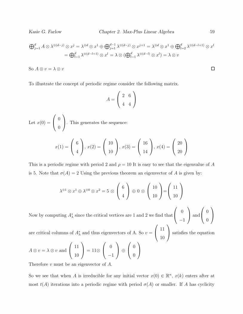
Kasie G. Farlow Chapter 2. Max-Plus Linear Algebra 59
⊕dj=1A⊗ λ⊗(d−j) ⊗ xj = λ⊗d ⊗ x1 ⊕
⊕d−1j=1 λ
⊗(d−j) ⊗ xj+1 = λ⊗d ⊗ x1 ⊕⊕d
l=2 λ⊗(d−l+1) ⊗ xl
=⊕d
l=1 λ⊗(d−l+1) ⊗ xl = λ⊗ (
⊕dl=1 λ
⊗(d−l) ⊗ xl) = λ⊗ v
So A⊗ v = λ⊗ v
To illustrate the concept of periodic regime consider the following matrix.
A =
2 6
4 4
Let x(0) =
0
0
. This generates the sequence:
x(1) =
6
4
, x(2) =
10
10
, x(3) =
16
14
, x(4) =
20
20
This is a periodic regime with period 2 and ρ = 10 It is easy to see that the eigenvalue of A
is 5. Note that σ(A) = 2 Using the previous theorem an eigenvector of A is given by:
λ⊗1 ⊗ x1 ⊕ λ⊗0 ⊗ x2 = 5 ⊗
6
4
⊕ 0 ⊗
10
10
=
11
10
Now by computing A∗λ since the critical vertices are 1 and 2 we find that
0
−1
and
0
0
are critical columns of A∗λ and thus eigenvectors of A. So v =
11
10
satisfies the equation
A⊗ v = λ⊗ v and
11
10
= 11⊗
0
−1
⊕
0
0
Therefore v must be an eigenvector of A.
So we see that when A is irreducible for any initial vector x(0) ∈ Rn, x(k) enters after at
most t(A) iterations into a periodic regime with period σ(A) or smaller. If A has cyclicity
Kasie G. Farlow Chapter 2. Max-Plus Linear Algebra 60
one then x(k) enters after at most t(A) iterations the eigenspace of A and x(k) behaves like
an eigenvector of A. If x(k) enters a periodic regime the effect of the initial condition doesn’t
fade away and the sequence x(k) does not ultimately behave like an eigenvector of A. So for
an irreducible matrix A we have determined the limiting behavior of x(k).
Chapter 3
Markov Chains
We indicated above that max-plus algebra arises as the “algebra of exponents” for quantities
having asymptotic expressions of the form esu as s → ∞; see Lemma 1. Such asymptotic
expressions arise in many places. One in particular is large deviations analysis in probability.
Large deviations analysis is concerned with the asymptotic decay of some probability pε which
depends on a vanishing parameter ε ↓ 0. The large deviations rate, if it exists, is defined by
V = − limε↓0
ε2 ln(pε).
Using our notation this is expressed as pε � e−V
ε2 , where V ≥ 0. For the connection with
standard max-plus algebra we replace −V by u (with u ≤ 0). (Otherwise we would need
to work in the min-plus algebra — we prefer to stay with the standard max-plus algebra
throughout this thesis.) We also replace ε−2 (ε ↓ 0) by s → ∞. This is because we want to
reserve ε for the max-plus additive identity ε = −∞, as is customary.
The book [27] of Wentzell and Freidlin is concerned with large deviations analysis of con-
tinuous processes (diffusions) on Euclidean spaces, and connected manifolds in general. In
Chapter 6 they show that for certain problems involving large time intervals, the analysis
can be reduced to the study of transitions between a finite number of compact subsets Ki.
The continuous process moves between the Ki in a way which can be approximated by a
61
Kasie G. Farlow Chapter 3. Markov Chains 62
Markov chain on a finite set of states, one for each Ki, having transition probabilities of the
form
pij � esuij , as s→ ∞. (3.1)
(This is after changing from their V, ε notation to our u, s notation as above.) Wentzell
and Freidlin establish several results for finite state Markov chains with this kind of asymp-
totic dependence. Our purpose in this chapter is to consider their Markov chain results as
applications of the max-plus linear algebra results described in the previous chapter.
We begin with the definition of a Markov chain. A random process X = {X0, X1...} is a
sequence of random variables which take values in some countable set L, called the state
space, is a Markov chain if it satisfies the Markov condition: P (Xn = s|X0 = x0, X1 =
x1, ....Xn−1 = xn−1) = P (Xn = s|Xn−1 = xn−1) for all n ≥ 1. The chain is described
by its transition probabilities P (Xn+1 = j|Xn = i) = pij. We want to consider a Markov
chain where the pij depend on a parameter s converging to infinity, in such a way that
lims→∞
s−1 ln(pij) = uij, in other words pij � esuij . To be transition probabilities of a Markov
chain we require pij ≥ 0 and∑
j pij = 1 for each i. This implies that uij ≤ e and⊕
j uij = e.
Note that in this chapter uij represents the weight of an edge from (i, j), not (j, i) as is the
customary max-plus interpretation.
For a Markov chain with such an asymptotic description the following three problems are
considered by Wetzell and Freidlin in [27]. We will describe the max-plus interpretation of
their results.
1. Determine the asymptotics of the stationary distribution.
2. For B ⊂ L, determine the asymptotic probability that the first contact with B occurs
at k ∈ B.
3. Determine the asymptotics of the expected number of steps to reach B ⊂ L.
In this chapter we consider these results from a max-plus perspective assuming that L is
finite.
Kasie G. Farlow Chapter 3. Markov Chains 63
3.0.1 Problem 1
In conventional algebra the stationary distribution is a vector v such that v = vP , with
vi ≥ 0 and∑vi = 1. It is unique if the probability matrix P is irreducible. It will follow
from Theorem 17 there exist wi for which we have vi � eswi. Our goal is to characterize
w = [wi] in max-plus terms. Now let U be the matrix of entries uij taken from the asymp-
totic description ,(3.1) of P . From Lemma 1 it follows that w = UT ⊗w. It is assumed in [27]
that P is irreducible (for each s ≥ 0). That does not necessarily imply that U is irreducible.
However if U is irreducible then P is irreducible. The fact that vi ≥ 0 and∑
i vi = 1 tells us
that⊕
wi = e and ε ≤ wi ≤ e.
We see that the exponents wi for the stationary distribution form a max-plus eigenvector for
UT with eigenvalue e = 0. Since uij ≤ e we know that all circuits have weight less then or
equal to e. Lemma 19 and the existence of an eigenvector tells us that there is a circuit of
average weight e. Thus UT has a maximal average circuit weight e, even though it may fail
to be irreducible. In the conventional sense we know that the stationary distribution v is
unique when the probability matrix P is irreducible. However even for an irreducible matrix
the max-plus eigenvector is not unique in general, see Example 1 below. Recall that if U is
irreducible the critical columns of UT are eigenvectors associated with eigenvalue λ = e and
every other eigenvector is a max-plus linear combination of the critical columns of U T . So
for an irreducible matrix we would like to know which linear combination of columns gives
us the correct eigenvector for the asymptotic description v? In general we would like to have
a concise max-plus characterization of the eigenvector w for the asymptotic description of v.
Although we do not know of a simple criteria which uniquely identifies w out of all max-plus
eigenvectors, we will be able to identify it constructively; see Theorem 17. In [1] Akian,
Bapat and Gaubert have some additional insight into this question. We will discuss their
results shortly.
Freidlin and Wentzell describe a graph theoretical approach to finding the stationary distri-

Kasie G. Farlow Chapter 3. Markov Chains 64
bution. In this approach they use B-graphs, which we will now define.
Definition 50. Suppose we have a subset B of a finite set L. A B-graph is a graph with
vertices L which consists of edges (m,n) with m ∈ L\B, n ∈ L and n 6= m and which satisfies
the following conditions:
1. every point m ∈ L\B is an initial point of exactly one edge.
2. for any point m ∈ L\B there is a sequence of edges leading from it to some point n ∈ B
The set of B-graphs is denoted by G(B). For g ∈ G(B) we define π(g) =∏
(m,n)∈g pmn where
pij are the transition probabilities for the Markov chain.
The following is Lemma 3.1 of Chapter 6 from [27], describing the stationary distribution in
terms of B-graphs.
Lemma 28. Consider an irreducible Markov chain with finite set of states L and transition
probabilities pij. Then the stationary distribution of the chain is vi = {(∑
i∈LQi)−1Qi}
where,
Qi =∑
g∈G{i} π(g).
The B-graphs translate directly into the max-plus setting. Since pij � esuij we have π(g) �
esρ(g) where ρ(g) =⊗
(i,j)∈g uij. Thus ρ(g) is the max-plus product of the weights of the
edges in g. Now we can state the max-plus version of the previous lemma.
Theorem 17. Consider an irreducible Markov chain with the set of finite states L and
transition probabilities pij � esuij . There exists a max-plus eigenvector w of UT whose kth
component is wk = wk −⊕
k∈L wk, where
wk =⊕
g∈G({k}) ρ(g).
Kasie G. Farlow Chapter 3. Markov Chains 65
Moreover vk � eswk where vk is the kth component of the unique stationary distribution of
P .
Proof. Applying Lemma 1 to the Qk of Lemma 28 we have that Qk � eswk. In other words
wk = lims→∞
s−1 ln(Qk) =⊕
g∈G({k}) ρ(g). Since vk = Qk∑
j Qjit follows that vk � eswk . Since
v = vP � es(w⊗U)(coordinate wise) the equation vP = v implies UT ⊗ w = w.
This theorem tells us that the max-plus version of Freidlin and Wentzell’s graph theoretical
construction of the stationary distribution produces the max-plus eigenvector w associated
with the asymptotic description of P . Note that w is the normalized vector of w in the
max-plus sense. So using this construction we can identify the right max-plus eigenvector
w that corresponds to the asymptotic description of the stationary distribution even though
max-plus eigenvectors are not unique. From Chapter 2, if U is irreducible, then w is a linear
combination of the critical columns of UT . However we do not have a procedure that tells
us which linear combination gives us the eigenvector w we are concerned with.
Below we emphasize the important results of Problem 1.
• Assuming the transition matrix P is an irreducible probability matrix, the stationary
distribution (normalized left Perron eigenvector) v does have exponential asymptotics
vi � eswi where w is a max-plus eigenvector of the max-plus matrix UT associated with
P .
• Although the eigenspace for the Perron eigenvalue of P (pij � esuij) is one-dimensional
(for each s), the max-plus eigenspace is not “one-dimensional” in general (i.e. there
can be other eigenvectors beyond c ⊗ w, c ∈ Rmax) except in the case that U has a
unique critical class ( see Lemma 23 on page 45).
• The correct max-plus eigenvector w for the asymptotic description of the stationary
distribution is determined by the max-plus matrix U . The max-plus version of the

Kasie G. Farlow Chapter 3. Markov Chains 66
B-graph gives us a graph theoretical procedure for finding w. What we don’t know is a
nice characterizing property that picks w out of all the possible max-plus eigenvectors
of UT . As far as we know this is an unsolved problem except for the case that U has
a unique critical class.
To get a better idea of what a B-graph is in max-plus, let’s consider the example illustrated
in Figure 3.1. In addition to the matrix U the figure shows the graph with the uij indicated
as edge weights.
U1=
0 0 −∞ −∞
−1 0 −9 −9
−∞ −6 0 −6
−∞ 0 0 0
1 2
3 4
0
−1
0
0
00
−9
−6
0−9
−6
0Figure 3.1: G(U1)
Let us calculate the set of graphs in G({1}) of the Markov chain with transition probabilities
uij below. Here L = {1, 2, 3, 4} and B = {1}. For each vertex in L\B = {2, 3, 4} we pick one
edge with that vertex as its initial point and so that there are no circuits for our selected edges.
(If we limit ourselves to g with ρ(g) > ε, then we can ignore edges with uij = ε.) Each such
selection of edges produces a g ∈ G({1}). For example g1 = {(2, 1), (3, 2), (4, 2)} make up
one graph in G({1}). We also have g2 = {(2, 1), (3, 2), (4, 3)} and g3 = {(3, 4), (4, 2), (2, 1)}
in G({1}).
To demonstrate Theorem 17 we will consider a few examples. Given a matrix U T1 obtained
from the asymtotics of P we will uses the previous theorem to find the max-plus eigenvector
w associated with P . We will also show that w satisfies the max-plus linear algebra results in
Chapter 2 about eigenvectors. As you will see the eigenspace of U T1 is rather complicated and
there is no obvious way to determine which linear combination of critical columns determine

Kasie G. Farlow Chapter 3. Markov Chains 67
the eigenvector w.
Example 6. Continuing with the example of Figure 3.1, we compute the max-plus eigenvec-
tor w for UT1 .
First we will compute w1 using Theorem 17. For each gj ∈ G({1}) we need to compute
ρ(gj). Note that this is just the max-plus product of the edges in gj for each i ∈ L.
ρ(g1) = −1 ⊗−6 ⊗ 0 = −7
ρ(g2) = −1 ⊗−6 ⊗ 0 = −7
ρ(g3) = −6 ⊗ 0 ⊗−1 = −7.
Therefore w1 = ⊕gj∈G({1})ρ(gj) = −7 ⊕−7 ⊕−7 = −7. Similarly we find that
w2 = −6, w3 = −9, w4 = −15.
Normalizing w in the max-plus sense we see that w =
−1
0
−3
−9
.
Now since w is an eigenvector of UT1 we should be able to write w as a max-plus linear
combination of the critical columns of UT1 . By Chapter 2 we find that
(UT1 )∗ =
0 −1 −7 −1
0 0 −6 0
−9 −9 0 0
−9 −9 −6 0
.
Notice that since the graph of U1 contains a loop of weight e on each vertex then V c(UT1 ) =
{1, 2, 3, 4} and

Kasie G. Farlow Chapter 3. Markov Chains 68
−1
0
−3
−9
=
−1
0
−9
−9
⊕ −3 ⊗
−7
−6
0
−6
. This shows us that w can be written as a linear
combination of the second and third critical columns of UT1 .
Example 7. : Consider the Markov chain described by matrix and graph in Figure 3.2.
U2=
0 −4 −∞ −∞ −∞ −9
0 0 −0 −∞ −∞ −∞
−∞ −5 0 −10 −∞ −∞
−∞ −∞ −0 0 0 −∞
−∞ −∞ −∞ −8 0 −9
0 −∞ −∞ −∞ 0 0
1 2
3 4
5 6
−4
0
0
0
00
0
0
0
6
−5
−90
−8
0
−10
00
Figure 3.2: G(U2)
We can calculate the stationary distribution using Theorem 17. We find that
w1 =⊕
g∈G({1}) ρ(g) = −13
{(2, 1), (3, 2), (4, 3), (5, 4), (6, 1)} is an example of a graph from G({1}) with ρ(g) = −13.
Similarly we find that w2 = −17, w3 = −17, w4 = −19, w5 = −14, w6 = −19.
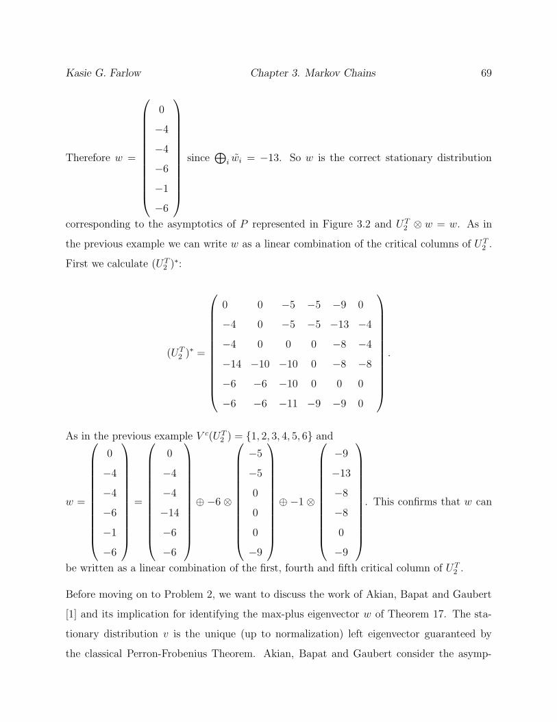
Kasie G. Farlow Chapter 3. Markov Chains 69
Therefore w =
0
−4
−4
−6
−1
−6
since⊕
i wi = −13. So w is the correct stationary distribution
corresponding to the asymptotics of P represented in Figure 3.2 and U T2 ⊗ w = w. As in
the previous example we can write w as a linear combination of the critical columns of U T2 .
First we calculate (UT2 )∗:
(UT2 )∗ =
0 0 −5 −5 −9 0
−4 0 −5 −5 −13 −4
−4 0 0 0 −8 −4
−14 −10 −10 0 −8 −8
−6 −6 −10 0 0 0
−6 −6 −11 −9 −9 0
.
As in the previous example V c(UT2 ) = {1, 2, 3, 4, 5, 6} and
w =
0
−4
−4
−6
−1
−6
=
0
−4
−4
−14
−6
−6
⊕ −6 ⊗
−5
−5
0
0
0
−9
⊕ −1 ⊗
−9
−13
−8
−8
0
−9
. This confirms that w can
be written as a linear combination of the first, fourth and fifth critical column of U T2 .
Before moving on to Problem 2, we want to discuss the work of Akian, Bapat and Gaubert
[1] and its implication for identifying the max-plus eigenvector w of Theorem 17. The sta-
tionary distribution v is the unique (up to normalization) left eigenvector guaranteed by
the classical Perron-Frobenius Theorem. Akian, Bapat and Gaubert consider the asymp-

Kasie G. Farlow Chapter 3. Markov Chains 70
totics of the Perron eigenvalue and eigenvector of irreducible non-negative matrices. They
consider the matrix A = lims→∞A(s)1/s which going back to Lemma 1 is the same as our
U = lims→∞ s−1 ln(A(s)) with U = ln(A). The natural logarithm maps their max-times
algebra on [0,∞) to the usual max-plus algebra on [−∞,∞). They consider matrices A(s)
which are nonnegative, but not necessarily probability matrices. That is very significant.
They offer the following example:
A(s) =
1 + cos(s)e−s e−2s
e−2s 1
.
The (right) Perron eigenvector turns out to be U(s) = (es cos(s) +√
4 + e2s cos2(s), 2).
We find that s−1 ln of the first coordinate is oscillatory as s → ∞. This shows that the
Perron eigenvector U(s) can be such that lims→∞ Ui(s)1/s fails to exist even though the
lims→∞Aij(s)1/s do exist. However their matrix A is not a probability matrix; neither the
rows nor the columns sum to 1. For irreducible probability matrices we know that the (left)
Perron eigenvector (which is the stationary distribution, when normalized) always does have
exponential asymptotics, because of applying Theorem 17. We can transpose their A(s)
(so that what was a left eigenvector becomes a right eigenvector) and then multiply the
rows by constants so that they sum to 1. The left Perron eigenvector now works out to
be U(s) =(
1+e2s+es cos(s)1+e2s , 1
)
. The point is that lims→∞ s−1 ln does exist for this. Thus the
asymptotic behavior of the Perron eigenvector is much better for probability matrices than
for nonnegative matrices in general. In Problem 1 we considered only probability matrices.
In the general case of [1], there need not exist a particular max-plus eigenvector U associated
with the Perron eigenvector of A(s); there could be multiple limit points of U(s)1/si as
s → ∞.In [1] they use U to represent the max-plus eigenvector which is not the same as
our max-plus probability matrix U . In [1] they do not consider the problem of identifying
the correct eigenvector if the eigenspace is multidimensional. In general there need not be
one. They simply focus on sufficient conditions for the max-plus eigenspace to be “one-
dimensional.” They do this first with just max-plus ideas in their Theorem 2 which is stated
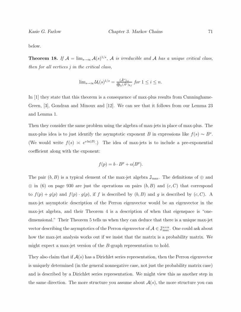
Kasie G. Farlow Chapter 3. Markov Chains 71
below.
Theorem 18. If A = lims→∞A(s)1/s, A is irreducible and A has a unique critical class,
then for all vertices j in the critical class,
lims→∞ Ui(s)1/s =
(A∗)ij⊕
k(A∗)kjfor 1 ≤ i ≤ n.
In [1] they state that this theorem is a consequence of max-plus results from Cunninghame-
Green, [3], Gondran and Minoux and [12]. We can see that it follows from our Lemma 23
and Lemma 1.
Then they consider the same problem using the algebra of max-jets in place of max-plus. The
max-plus idea is to just identify the asymptotic exponent B in expressions like f(s) ∼ Bs.
(We would write f(s) � es ln(B).) The idea of max-jets is to include a pre-exponential
coefficient along with the exponent:
f(p) = b ·Bp + o(Bp).
The pair (b, B) is a typical element of the max-jet algebra Jmax. The definitions of ⊕ and
⊗ in (6) on page 930 are just the operations on pairs (b, B) and (c, C) that correspond
to f(p) + g(p) and f(p) · g(p), if f is described by (b, B) and g is described by (c, C). A
max-jet asymptotic description of the Perron eigenvector would be an eigenvector in the
max-jet algebra, and their Theorem 4 is a description of when that eigenspace is “one-
dimensional.” Their Theorem 5 tells us when they can deduce that there is a unique max-jet
vector describing the asymptotics of the Perron eigenvector of A ∈ Jn×nmax . One could ask about
how the max-jet analysis works out if we insist that the matrix is a probability matrix. We
might expect a max-jet version of the B-graph representation to hold.
They also claim that if A(s) has a Dirichlet series representation, then the Perron eigenvector
is uniquely determined (in the general nonnegative case, not just the probability matrix case)
and is described by a Dirichlet series representation. We might view this as another step in
the same direction. The more structure you assume about A(s), the more structure you can

Kasie G. Farlow Chapter 3. Markov Chains 72
expect the eigenvector to have. We have already seen this if the structure is a probability
matrix. We should expect the same thing if the structure is in terms of a more specific type
of asymptotic description or series representation.
3.0.2 Problem 2
As in Problem 1 we will consider a Markov chain on a state space L with B ⊂ L. Let
D = L \B and pick k ∈ B. We want to determine the probability of starting at state i ∈ D
and hitting B first at state k. In conventional algebra for i ∈ D we let hi be the probability
that the chain starting at i ∈ D will first reach B at k ∈ B. Denote the size of D by d. The
hi i ∈ D are characterized by the equation hi =∑
j∈D pijhj + pik, i ∈ D. So h is a d × 1
vector. We define PD = [Pij] where i, j ∈ D and b(k) = [pik] with i ∈ D. Then we have the
matrix equation h = PDh + bk. According to Lemma 3.3 from Chapter 6 of [27], hi � esai
for some ai ∈ Rmax. Continuing to assume P is an irreducible matrix with pij � esuij we
apply Lemma 1 to see that for each i ∈ D, ai = [⊕
j∈D uij ⊗ aj ]⊕uik. As a max-plus matrix
equation this is a = [UD ⊗ a] ⊕ ck where ck = [uik], i ∈ D.
We know that the average circuit of UD must be less then or equal to e = 0, since −∞ ≤
uij ≤ e. By Theorem 7 on page 31 the equation a = [UD ⊗ a] ⊕ ck has at least one
solution. But in general this solution in not unique unless the maximal average circuit in
UD is negative. So the question is how to identify the correct solution for the asymptotic
description of hi.
As in problem 1, Freidlin and Wentzell have a graph theoretical technique for determining
the probability hi described above. Again we will consider the set of B-graphs. We need to
consider a subset of G(B) denoted by Gik(B) where i ∈ D and k ∈ B.
Definition 51. The set of Gik(B) graphs are a subset of the B-graphs such that each graph
is Gik(B) has the following properties:
• They do not contain circuits.

Kasie G. Farlow Chapter 3. Markov Chains 73
• For each vertex in D there is a sequence of edges going into B.
• There exists a sequence of edges from i to k.
• The remaining vertices j 6= i in D may be included in this sequence of edges or may be
contained in a sequence of edges ending in B.
The following is a restatement of Lemma 3.3 found in Chapter 6 of [27].
Lemma 29. Given an irreducible Markov chain on a finite state space L, the probability that
chain starting at i ∈ D = L\B hits B ⊂ L first at k ∈ B is given by:
hi =∑
g∈Gik(B) π(g)∑
g∈G(B) π(g).
Now we state the max-plus version of the previous lemma.
Theorem 19. Given an irreducible Markov chain on a finite state space L and transition
probabilities pij � esuij where U is irreducible, let h be the probability of first hitting B at
k ∈ B. Then hi � esai where ai =⊕
g∈Gik(B) ρ(g) −⊕
g∈G(B) ρ(g) for each i ∈ L\B. This is
the solution to a = [UD ⊗ a] ⊕ ck which provides the asymptotic description of h.
We have added the extra hypothesis that U is irreducible to guarantee that⊕
g∈G(B) ρ(g) 6= ε.
Note that if U is irreducible,⊕
g∈G(B) ρ(g) > ε.
Proof. Using Lemma 1 and the same notation from problem 1, we see that the description
of hi in Lemma 29 implies that hi � esai where ai =⊕
g∈Gik(B) ρ(g) −⊕
g∈G(B) ρ(g).
We have already observed that a = [ai], i ∈ D is a solution of a = [UD ⊗a]⊕ ck. Theorem 19
provides an explicit construction of the correct solution for the asymptotic description of h.
To illustrate the procedure of finding the probability of hitting B ⊂ L first at k ∈ B we will
consider the examples of Figure 3.1 and Figure 3.2 again.
Kasie G. Farlow Chapter 3. Markov Chains 74
Example 8. Consider the example of Figure 3.1. Let B = {1, 3} and D = {2, 4} and k = 3.
We see that
⊕
g∈G23(B) ρ(g) = u24 + u43 = −9,⊕
g∈G43(B) ρ(g) = u43 + u21 = −1⊕
g∈G(B) ρ(g) = u21 + u43 = −1.
Therefore
a =
−8
0
.
We can check directly that a = (UD1 ⊗a)⊕ck:
0 −9
0 0
⊗
−8
0
⊕
−9
0
=
−8
0
.
Example 9. Consider the example of Figure 3.2. Let B = {4, 5, 6} and k = 4.
We see that
⊕
g∈G16(B) ρ(g) = u12 + u23 + u34 = −14,⊕
g∈G26(B) ρ(g) = u12 + u23 + u34 = −14,⊕
g∈G36(B) ρ(g) = u12 + u23 + u34 = −14⊕
g∈G(B) ρ(g) = u32 + u21 + u16 = −11.
Therefore
a =
−3
−3
−3
.
This is the solution that corresponds to the asymptotics of h. Again we check that a =
[UD2 ⊗ a] ⊕ ck directly.
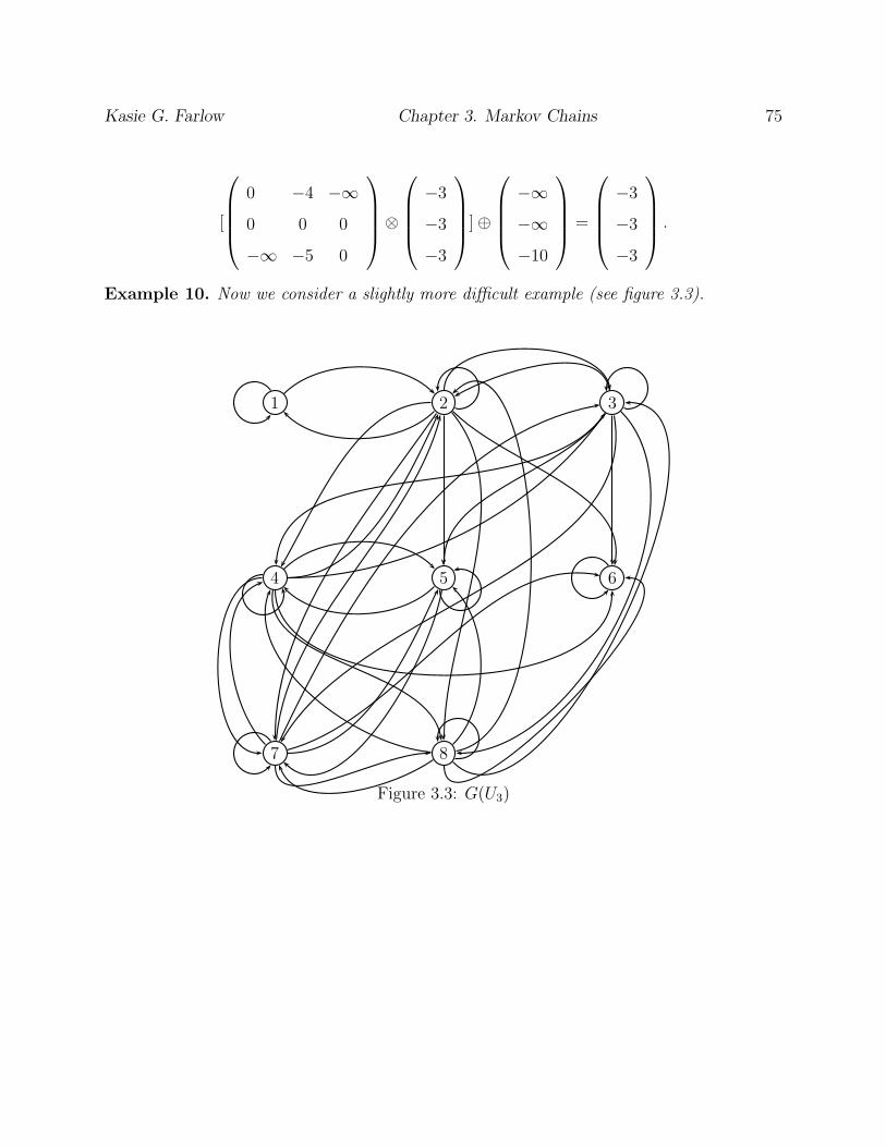
Kasie G. Farlow Chapter 3. Markov Chains 75
[
0 −4 −∞
0 0 0
−∞ −5 0
⊗
−3
−3
−3
] ⊕
−∞
−∞
−10
=
−3
−3
−3
.
Example 10. Now we consider a slightly more difficult example (see figure 3.3).
1 2 3
4 5 6
7 8
Figure 3.3: G(U3)

Kasie G. Farlow Chapter 3. Markov Chains 76
U3 =
0 −0 −∞ −∞ −∞ −∞ −∞ −∞
−1 0 −9 −9 −10 −9 −12 −8
−∞ −6 0 −6 −7 −6 −7 −7
−∞ 0 0 0 −5 −4 −7 −5
−∞ 0 0 0 0 0 −5 0
−∞ −3 0 −3 −7 0 −5 −5
−∞ 0 0 0 −5 0 0 0
−∞ 0 −8 −8 −10 −9 −11 0
Let B = {5, 6, 7, 8} and k = 5. We see that
⊕
g∈G15(B) ρ(g) = −16,⊕
g∈G25(B) ρ(g) = −16,⊕
g∈G35(B) ρ(g) = −15,⊕
g∈G45(B) ρ(g) = −15⊕
g∈G(B) ρ(g) = −14
a =
−2
−2
−1
−1
.
Again we check that a also satisfies the equation a = [UD3 ⊗ a] ⊕ ck:
[
0 −0 −∞ −∞
−1 0 −9 −9
−∞ −6 0 −6
−∞ 0 0 0
⊗
−2
−2
−1
−1
] ⊕
−∞
−10
−7
−5
=
−2
−2
−1
−1
.
Kasie G. Farlow Chapter 3. Markov Chains 77
3.0.3 Problem 3
As in Problem 1 and 2 we have a Markov chain on a state space L with pij � esuij . In
this problem we will compute the expected number of steps to reach B ⊂ L from an initial
state i ∈ D = L\B. Let nB be the smallest n for which Xn ∈ B and mB(i) = Ei[nB]. In
conventional algebra we have for i ∈ L\B, mB(i) = 1 +∑
j 6∈B pijmB(j) where 1 = [1]i∈D. If
PD = [pij]i,j∈D and mB = [mB(i)]i∈D then mB = 1+PDmB . Using Lemma 1 as in Problem
1 and 2 the conventional equation converts to a max-plus equation, provided mB(i) � eszi
and pij = esuij . So we get z = e ⊕ [UD ⊗ z], where e is the max-plus vector of all zeros. By
Theorem 7 on page 31 since U has circuits of average weight less then or equal to e then one
solution is z = (UD)∗ ⊗ e. But, as in Problem 1 and Problem 2, the solution z found using
Theorem 7 is not unique unless the maximal average circuit in UD is negative. Therefore
that solution may not be the correct solution corresponding to the asymptotic description
of mB. We will consider Freidlin and Wentzell’s graph theoretical approach to solving this
problem (in the conventional sense) and find the max-plus analogue of their results. Here is
the result from [27](Lemma 3.4 of Chapter 6).
Lemma 30. Given an irreducible Markov chain on a finite state space L the expected number
of steps until the first entrance into B ⊂ L starting at i ∈ D is given by
mB(i) =
∑
g∈G(B∪{i}) π(g)+∑
i∈D,j 6=i
∑
g∈Gij (B∪{j}) π(g)∑
g∈G(B) π(g)
Note that the numerator in the equation for mB(i) contains graphs without cycles and d− 1
edges (m,n), m ∈, n ∈ L,m 6= n such that the sequence of edges does not contain a path
from i into B. From this lemma we now derive the following max-plus theorem that gives
the correct solution to z = e ⊕ [UD ⊗ z] that corresponds to mB(i) above.
Theorem 20. Under the same hypotheses as Theorem 19 with mB(i) � eszi,
zi = [⊕
g∈G(B∪{i}) ρ(g)] ⊕ [⊕
i∈D,j 6=i
⊕
g∈Gij(B∪{j}) ρ(g)] −⊕
g∈G(B) ρ(g)
Kasie G. Farlow Chapter 3. Markov Chains 78
is the expected number of steps until the first entrance into B ⊂ L starting at i ∈ D where
z = [zi]i∈D satisfies z = e⊕ [UD ⊗ z].
Proof. As in the Theorem 19 we just apply Lemma 1 to Lemma 30.
Now let’s look at a few examples that demonstrate the previous result for Problem 3.
Example 11. Consider again the example of Figure 3.1 with B = {3, 4}.
First we see that
⊕
g∈G(B∪{1}) ρ(g) = u21 = −1 and⊕
g∈G(B∪{2}) ρ(g) = u12 = 0.
Next we consider the Gij(B ∪ {j}):
⊕
g∈G12(B∪{2}) ρ(g) = u12 = 0 and⊕
g∈G21(B∪{1}) ρ(g) = u21 = −1.
Since⊕
g∈G(B) ρ(g) = −9 we conclude that
z = [
−1
0
⊕
0
−1
] −
−9
−9
=
9
9
.
We check that z satisfies the equation z = e ⊕ [UD1 ⊗ z]:
z =
9
9
=
0
0
⊕ [
0 0
−1 0
⊗
9
9
].
Example 12. Consider the example of figure 3.2 with B = {4, 5, 6}.
First we see that:
Kasie G. Farlow Chapter 3. Markov Chains 79
⊕
g∈G(B∪{1}) ρ(g) = u21 + u32 = −4⊕
g∈G(B∪{2}) ρ(g) = u12 + u32 = −9⊕
g∈G(B∪{3}) ρ(g) = u12 + u23 = −4.
Next we consider the Gij(B ∪ {j}).
For i = 1 we have
⊕
g∈G12(B∪{2}) ρ(g) = u12 + u34 = −9 and⊕
g∈G13(B∪{3}) ρ(g) = u21 + u23 = −4.
For i = 2 we have
⊕
g∈G21(B∪{1}) ρ(g) = u21 + u32 = −5 and⊕
g∈G23(B∪{3}) ρ(g) = u21 + u23 = −4.
For i = 3 we have
⊕
g∈G31(B∪{1}) ρ(g) = u32 + u21 = −5 and⊕
g∈G32(B∪{2}) ρ(g) = u32 + u12 = −9.
Finally we see that⊕
g∈G(B) ρ(g) = −11. Therefore we conclude that
z = [
−5
−9
−4
⊕
−4
−4
−5
] −
−11
−11
−11
=
7
7
7
.
We find that z does indeed satisfy the required max-plus equation:
z =
7
7
7
=
0
0
0
⊕ [
0 −4 −∞
−0 0 0
−∞ −5 0
⊗
7
7
7
].
Chapter 4
Concluding Remarks
This thesis has given the reader a survey of max-plus algebra which focuses on the linear
algebra aspects of max-plus algebra. We also described how we could apply these results to
several results by Wentzell and Freidlin for finite state Markov chains with an asymptotic
dependence. We would like to consider directions for future investigation of max-plus. Below
we describe a few possibilities.
1. One obvious direction is the issue we came across in Problem 1 of Chapter 3. We would
like to try and develop a nice max-plus characterization of the stationary distribution
produced in Theorem 17.
2. Professor Marianne Akian, who gave us some insight into our issue in Problem 1, has
developed a theory of max-plus probabilities motivated by dynamical programming
and large deviations [12]. We might want to explore her research and continue in this
direction with our work in max-plus algebra.
3. The authors in [3] briefly mentioned the max-plus analogues of Brownian motion and
probability laws such as the central limit theorem. This is an intriguing avenue to
pursue further.
80
Kasie G. Farlow Chapter 4. Concluding Remarks 81
4. As previously mentioned this thesis focused on the finite dimensional linear algebra
results. Another path to take is to explore the infinite dimensional max-plus algebra.
Above we briefly discussed this and what we called max-plus function analysis. We
may consider proceeding in this direction and the path Professor McEeaney has taken
with max-plus algebra.
Bibliography
[1] M Akian R. Bapat, and S. Gaubert, Asymptotics of the perron eigenvalue and eigen-
vector using max-algebra C. R. Acad. Sci. Paris, t.327, Seire 1,(1998) pp. 927–932 .
[2] M.Akian, R. Bapat, S. Gaubert, Max-plus algebras, Chapter 25 in the Handbook of
Linear Algebra, L. Hogben, R. Brualdi, A. Greenbaum, and R. Mathias (editors),
Discrete Mathematics and Its Applications, 39, Chapman and Hall, 2007.
[3] F. Baccelli, G. Cohen, G.L. Olsder and J.P Quadrat, Syncronization and Linear-
ity, Wiley, New York, 1992.
[4] R.B. Bapat, David P. Standford, P. Van Den Driessche, Pattern, properties and spectral
inequalities in max algebra, SIAM. J Matrix Anal Appl. 16 No 3 (1985), pp. 964-976.
[5] J.G. Braker and G.J. Olsder, The power algorithm in the max algebra, Linear Algebra
and its Applications. 182 (1993) pp. 67-89.
[6] Bart De Schutter, Bart De Moor A note on the Characteristice Equation in the Max-Plus
Algebra, Linear Albebra and its Applications. 261 (1997), pp. 237-250.
[7] Bart De Shutter, On the ultimate behavior of the sequence of consecutive powers of
a matrix in the max-plus algebra, Linear Algebra and it Applications. 30 (2000), pp.
103-117.
[8] R.A. Cuninghame-Green and P Butkovic, Bases in max-algebra, Linear Algebra and its
Applications, 389 (2004), pp. 104-120.
82
Kasie G. Farlow Bibliography 83
[9] R.A. Cuninghame-Green, Minimax Algbera Lecture notes in Economics and
Mathematical Systems. 166 Springer, 1979.
[10] Wendell H. Fleming and William M. McEneaney, A max-plus based algorithm for a
Hamilton-Jacobi-Bellman equation of nonlinear filtering, SIAM J. Control Optim. 38
(2000), pp. 683–710.
[11] Wendell H. Fleming and H. Mete Soner, Controlled Markov Processes and
Viscosity Solutions, Springer-Verlag, New York, 1993.
[12] Gaubert,S, Methods and applications of (max,+) linear algebra, STACS 1997, Lecure
Notes in Computer Science 500, Springer-Verlag, Berlin, (1997), pp. 261-282.
[13] M. Gondran, and M.Minoux, Linear algebra in diodids: A survey of recent results,
Annals of Discrete Mathematics, 19 (1984), pp. 147-164.
[14] M.Gondran and M.Minoux, L’independence lineaire dans les dioides, Bulletin De La
Direction Des Etudes et Recherches Series C. 1, (1978), pp. 67-90.
[15] R.G. Halburd, N.J. Southall, Tropical nevanlinna theory and ultra -disctete equations,
Loughborough University, 2007.
[16] B. Heidergot, G.J.Olsder, J.Woude, Max Plus at Work, Princeton Universty Press,
New Jersey, 2006.
[17] T.W. Hungerford, Algebra: Graduate texts in mathematics, Springer-Verlag,
New York, 1974.
[18] S.C. Kleene. Representation of events in nerve sets and finite automa, Automata Stud-
ies, Annals of Mathematical Studies. No.34 (1956), pp. 3-41.
[19] G.L. Litvinov, V.P. Maslov and G.B. Shipz, Idempotent functional analysis: an alge-
braic approach, Mathematical Notes. 69(5): (2001), pp. 696-729.
Kasie G. Farlow Bibliography 84
[20] William M. McEneaney, Max-Plus Methods for Nonlinear Control and Es-
timation, Birkhauser, Boston, 2006.
[21] William M. McEneaney, Max-plus eigenvector representations for solution of nonlinear
H∞ problems: basic concepts, IEEE Trans. Automat. Control 48 (2003), pp. 1150–1163.
[22] William M. McEneaney, Max-plus eigenvector methods for nonlinear H problems: error
analysis, SIAM J. Control Optim. 43 (2004), pp. 379–412.
[23] William M. McEneaney, A curse-of-dimensionality-free numerical method for solution
of certain HJB pdes, SIAM J. Control Optim. 46 (2007), pp. 1239–1276.
[24] G.J. Olsder, On the Characteristic Equation and Minimal Realizations for Disctrete-
event Dynamic Systmes, Lecture Notes in Control and Inform. Sci. 83 (1986), pp.189-
2001.
[25] G.J. Olsder and C. Roos,Cramer and Cayley-Hamilton in the max-algebra, Linear Al-
gebra and its Applications. 101 (1988), pp. 87-108.
[26] E. Wagneur, Moduloids and pseudomodules.1.dimesion theory, Discrete Math. 98(1991),
pp. 57-73.
[27] M. I. Freidlin and A. D. Wentzell, Random Perturbations of Dynamical Sys-
tems, Springer-Verlag, New York, 1984.
Kasie G. Farlow List of Symbols 85
List of Figures:
• ⊕,⊗: pg 8
• E : pg 12
• G(A) : pg 14 item ‖p‖l : pg 14
• ‖p‖w : pg 14
• ‖c‖w
‖c‖l: pg 15
• A⊗k : pg 15
• P (i, j, k) : pg 15
• A∗ : pg 16
• A+ : pg 16
• perm(A) : pg 23
• dom(A): pg 23
•
∆1(A)
∆2(A)
: pg 26
• C(A) : pg 35
• Gc(A) : pg 35
• Aλ : pg 35
• V c(a) : pg 37
• Sλv(A) : pg 39
• Vλ(A) : pg 42

Kasie G. Farlow List of Symbols 86
• Aσσ : pg 45
• G(B) : pg 64
• π(g) : pg 64
• ρ(g) : pg 64
• Gij(B) : pg 73