MAXIMIZING PEAK CAPACITY-

Peak capacity is affected by: —Gradient duration (tg) —Flow rates (F) —Column length (L) —Particle size (dp)

Recommended starting flow rates, to be adjusted according to the separation.

We see above that for a 32 minute gradient run on a 4.6 x 20 mm ISTM column, a flow rate of 1.1 mL/min is predicted to maximize the peak capacity. But, for a 4 minute gradient, a fast flow rate of 2.6 mL/min is predicted for maximum peak capacity. We can now run experiments to test the theory.

We observe above that a flow rate of 3 mL/min offers the best solution as far as peak capacity, sol-vent consumption and fast separations.

-0.005

0.000

0.005

0.010

0.015

0.020

0.025

0.030

0.035

0.00 0.10 0.20 0.30 0.40 0.50 0.60 0.70 0.80 0.90 1.00 1.10 1.20 1.30 1.40 1.50

tg

w ww w

w

wt

1P g+=

Gradient Duration

Peak Width-0.005

0.000

0.005

0.010

0.015

0.020

0.025

0.030

0.035

0.00 0.10 0.20 0.30 0.40 0.50 0.60 0.70 0.80 0.90 1.00 1.10 1.20 1.30 1.40 1.50

tg

w ww w

w

wt

1P g+=

Gradient Duration

Peak Width

Peak capacity is a measure of the separation power of a gradient on a particular column.

1tt∆cB

∆cB4

tL

Dcd

LtDbda

L

1P

g

0

0M

2p0

Mp

+⋅⋅

⋅⋅⋅

⋅+⋅⋅+⋅

+=

We can now generate a 3-dimensional plot to examine how the gradient time and flow rate effect the peak capacity of a separation.

wt

1P g+=Start with the simple equation for peak capacity

Make a few substitutions

Neue, U. D., Mazzeo, J. R. J. Sep. Sci. 2001, 24, 921-929.Cheng, Y-F., Lu, Z., Neue, U. Rapid Commun. Mass Spectrom. 2001, 15, 141-151.

0.0 0.1 0.1 0.1 0.2 0.3 0.4 0.5 0.7 1.1 1.5 2.1 3.0 4.2 6.0 8.41.00

2.00

4.008.00

16.0032.00

0

50

100

150

Peak

Cap

acity

Flow Rate [mL/min]

Gradient Duration [min]

Long gradients require

slow flow rates

1.1 mL/min

4.6 x 20 mm, 3.5 µm Column

32 minute gradient

0.0 0.1 0.1 0.1 0.2 0.3 0.4 0.5 0.7 1.1 1.5 2.1 3.0 4.2 6.0 8.41.00

2.00

4.008.00

16.0032.00

0

50

100

150

Peak

Cap

acity

Flow Rate [mL/min]

Gradient Duration [min]

4.6 x 20 mm, 3.5 µm Column

Short gradientsrequire FAST

flow rates

2.6 mL/min

4 minute gradient

2 mL/min790 psi

3 mL/min1200 psi

4 mL/min1650 psi

AU

0.000

0.050

0.080

Minutes0.20 0.40 0.60 0.80 1.00 1.20 1.40 1.60 1.80 2.00 2.20 2.40 2.60 2.80 3.00 3.20 3.40 3.60 3.80 4.00

AU

0.000

0.050

0.080

Minutes0.20 0.40 0.60 0.80 1.00 1.20 1.40 1.60 1.80 2.00 2.20 2.40 2.60 2.80 3.00 3.20 3.40 3.60 3.80 4.00

AU

0.000

0.050

0.070

Minutes0.20 0.40 0.60 0.80 1.00 1.20 1.40 1.60 1.80 2.00 2.20 2.40 2.60 2.80 3.00 3.20 3.40 3.60 3.80 4.00

AU

0.000

0.050

0.070

Minutes0.20 0.40 0.60 0.80 1.00 1.20 1.40 1.60 1.80 2.00 2.20 2.40 2.60 2.80 3.00 3.20 3.40 3.60 3.80 4.00

AU

0.000

0.050

Minutes0.20 0.40 0.60 0.80 1.00 1.20 1.40 1.60 1.80 2.00 2.20 2.40 2.60 2.80 3.00 3.20 3.40 3.60 3.80 4.00

AU

0.000

0.050

Minutes0.20 0.40 0.60 0.80 1.00 1.20 1.40 1.60 1.80 2.00 2.20 2.40 2.60 2.80 3.00 3.20 3.40 3.60 3.80 4.00

1 2 34

5

1 2 34

5

1 2 34

5

P = 32

P = 39

P = 41

XTerra® MS C18 4.6 x 20 mm IS™, 3.5 µm

1 mL/min384 psi

AU

0.000

0.090

Minutes0.20 0.40 0.60 0.80 1.00 1.20 1.40 1.60 1.80 2.00 2.20 2.40 2.60 2.80 3.00 3.20 3.40 3.60 3.80 4.00

P = 231 2 3

4

5

AU

0.000

0.090

Minutes0.20 0.40 0.60 0.80 1.00 1.20 1.40 1.60 1.80 2.00 2.20 2.40 2.60 2.80 3.00 3.20 3.40 3.60 3.80 4.00

P = 231 2 3

4

5

0.63 mL/min2.1 x 20 mm1.28 mL/min3.0 x 20 mm2.16 mL/min3.9 x 20 mm3.0 mL/min4.6 x 20 mmFlow RateColumn Dimensions

0.63 mL/min2.1 x 20 mm1.28 mL/min3.0 x 20 mm2.16 mL/min3.9 x 20 mm3.0 mL/min4.6 x 20 mmFlow RateColumn Dimensions

SCALING SEPARATIONS- To successfully scale separations run on long columns to the 20 mm length columns, we use the following equation to scale the gradient:

We developed this separation on a long column:

Compounds: 1. Caffeine 2. Aniline 3. N-Methylaniline 4. 2-Ethylaniline 5. 4-Nitroanisole 6. N-N-Dimethylaniline Conditions: Column: XTerra® MS C18, 4.6 x 150 mm, 5 µm Mobile Phase A: Water Mobile Phase B: Acetonitrile Mobile Phase C: 100 mM NH4HCO3, pH 10 Flow Rate: 1.4 mL/min Gradient: Time Profile (min) %A %B %C 0.0 80 10 10 20.0 50 40 10 21.0 80 10 10 25.0 80 10 10 Injection Volume: 10 µL Sample concentration: 20 µg/mL Temperature: 30°C Detection: UV @ 254 nm Sampling Rate: 5 pts/sec Filter: 0 (no filter) Instrument: Alliance® 2695 with 996 PDA

To scale the separation to a 20 mm column, we first scale the gradient using the previous equation: We ran a 2.7 minute gradient on a 4.6 x 20 mm IS™, 3.5 µm column at 3 mL/min for a total cycle time of 4 minutes – down from 25 minutes! We further optimized the separation for a total cycle time of 3 minutes.

LC/MS SEPARATIONS-

To scale a gradient

2g1g1

2 ttLL

=×L1 = Long column lengthL2 = Short column length

tg1 = Gradient time on long columntg2 = Gradient time on short column

2

4

3

56

1

AU

0.00

0.02

0.04

0.06

Minutes

0.00 2.00 4.00 6.00 8.00 10.00 12.00 14.00 16.00 18.00 20.00

AU

0.00

0.02

0.04

0.06

Minutes

0.00 2.00 4.00 6.00 8.00 10.00 12.00 14.00 16.00 18.00 20.00

Six peaks resolved in a cycle time of 25 minutes.

Can we go faster?

min7.2min2015020 =×

mmmm

AU

0.00

0.02

0.04

0.06

0.08

0.10

Minutes0.00 0.20 0.40 0.60 0.80 1.00 1.20 1.40 1.60 1.80 2.00 2.20 2.40 2.60

AU

0.00

0.02

0.04

0.06

0.08

0.10

Minutes0.00 0.20 0.40 0.60 0.80 1.00 1.20 1.40 1.60 1.80 2.00 2.20 2.40 2.60

24

3

56

1 2 minute elution!

0.00 0.20 0.40 0.60 0.80 1.00Time0

100

%

0

100

%

0

100

%

0

100

%

1: Scan ES+ TIC

1.15e90.88

0.65

0.59

1: Scan ES+ 263

4.05e70.590.65

0.88

1: Scan ES+ 262

1.19e80.65

1: Scan ES+ 233

1.28e80.89

0.00 0.20 0.40 0.60 0.80 1.00Time0

100

%

0

100

%

0.00 0.20 0.40 0.60 0.80 1.00Time0

100

%

0

100

%

0

100

%

0

100

%

1: Scan ES+ TIC

1.15e9

0

100

%

0

100

%

1: Scan ES+ TIC

1.15e90.88

0.65

0.59

1: Scan ES+ 263

4.05e70.590.65

0.88

1: Scan ES+ 262

1.19e8

0.88

0.65

0.59

1: Scan ES+ 263

4.05e70.590.65

0.88

1: Scan ES+ 262

1.19e80.65

1: Scan ES+ 233

1.28e8

0.65

1: Scan ES+ 233

1.28e80.89

Analytes MWCinoxacin 262.2Oxolinic Acid 261.2Nalidixic Acid 232.2

ConditionsColumn: AtlantisTM dC18, 2.1x 20 mm IS™, 3 µmMobile Phase A: H2OMobile Phase B: MeOHMobile Phase C: 1% HCOOH in H2OFlow Rate: 0.4 mL/minGradient: Time Profile

(min) %A %B %C 0.0 50 40 101.0 30 60 10

Injection Volume: 2 µLSample Concentration: 10 µg/mLTemperature: 30 oCInstruments: Alliance® 2795 and Waters ZQTM

Cinoxacin

Nalidixic acid

Oxolinic acid

With a 2.1 mm i.d. column,lower flow rates enable DIRECT flow into the MS and the separation is only 1 minute long!

No flow splitting!

1 Minute!

TIC

Second peak is isotope from oxolinic acid

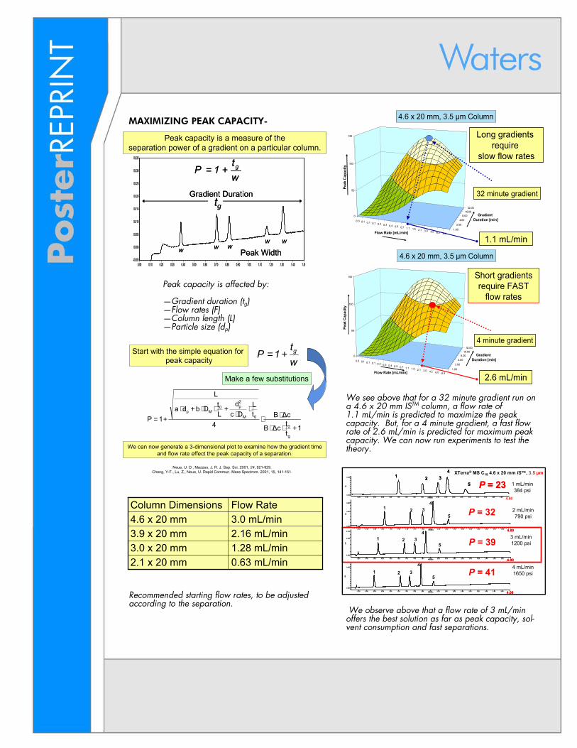
COST SAVINGS CALCULATIONS- Assume that an HPLC is running about 67% of the year, or 4000 hr. We used the previous separation as an example. We can calculate the solvent cost savings. Assume that 5000 samples need to be ana-lyzed for a study.

4.6 x 150 mm 4.6 x 20 mm IS™

Cycle time (min) 25 3

# of Samples Run per Year

9600 80,000

This is 8.3x as many samples run in one year, on ONE HPLC by using an intelligently designed column!

4.6 x 150 mm 4.6 x 20 mm IS™

Cycle time (min) 25 3

Total time for 5000 samples (hours)

2083 (87 days) 250 (10 days)

Flow rate (mL/min) 1.4 3

Total solvent consumption (L) 175 45

Amount ACN Consumed (L)(~ 25% is ACN)

43.75 11.25

Cost for ACN ($42.50/L) $1860 $480

Cost for waste disposal (~$2.50/L)

$438 $113

Total solvent costs $2298 $593

Cost savings of $1705 in solvents alone. *Additional cost savings in overhead.

To scale a flow rate for different internal diameters

( )( ) 212

1

22 FFx

dd

=

d1 = Diameter of original columnd2 = Diameter of second columnF1 = Flow rate on original columnF2 = Flow rate on second column

Scale from a 4.6 mm i.d. to a 2.1 mm i.d. column.

Flow rate scales from 3 mL/min to 0.6 mL/min.

$23$438Cost for waste disposal (~$2.50/L)

$119$2298Total solvent costs

2.2543.75Amount ACN Consumed (L)(~ 25% is ACN)

$96$1860Cost for ACN ($42.50/L)

0.61.4Flow rate (mL/min)

9175Total solvent consumption (L)

2.1 x 20 mm IS™4.6 x 150 mm

$23$438Cost for waste disposal (~$2.50/L)

$119$2298Total solvent costs

2.2543.75Amount ACN Consumed (L)(~ 25% is ACN)

$96$1860Cost for ACN ($42.50/L)

0.61.4Flow rate (mL/min)

9175Total solvent consumption (L)

2.1 x 20 mm IS™4.6 x 150 mm

Cost savings of $2179!

2.1 x 20 mm IS™, 3.5 µm

AU

0.00

0.02

0.04

0.06

0.08

0.10

Minutes0.00 0.20 0.40 0.60 0.80 1.00 1.20 1.40 1.60 1.80 2.00

1

23

4 5 6

2.1 x 20 mm IS™, 3.5 µm

AU

0.00

0.02

0.04

0.06

0.08

0.10

Minutes0.00 0.20 0.40 0.60 0.80 1.00 1.20 1.40 1.60 1.80 2.00

AU

0.00

0.02

0.04

0.06

0.08

0.10

Minutes0.00 0.20 0.40 0.60 0.80 1.00 1.20 1.40 1.60 1.80 2.00

1

23

4 5 6

For even further cost savings, we can scale the inner diameter from a 4.6 to a 2.1 mm and calculate the savings:

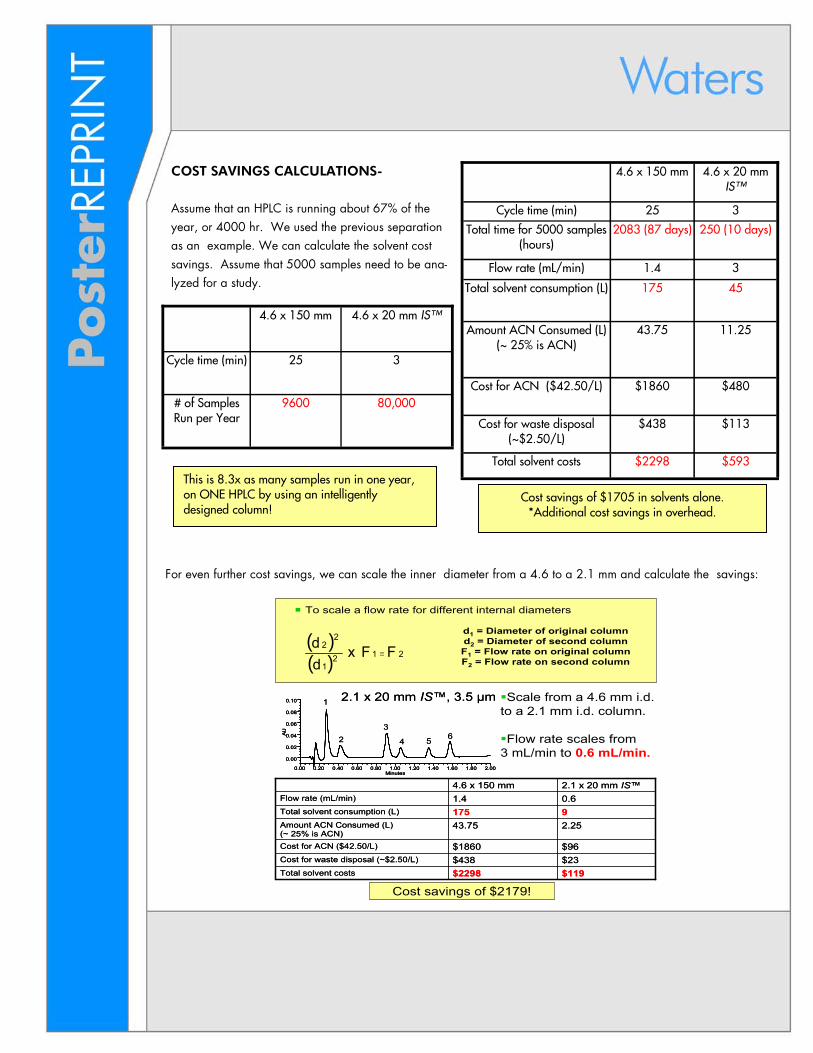
COMPARISON TO MONOLITH- We ran a separation originally run on the monolith, modified the mobile phase, and ran it on the ISTM column. We achieved a better separation.

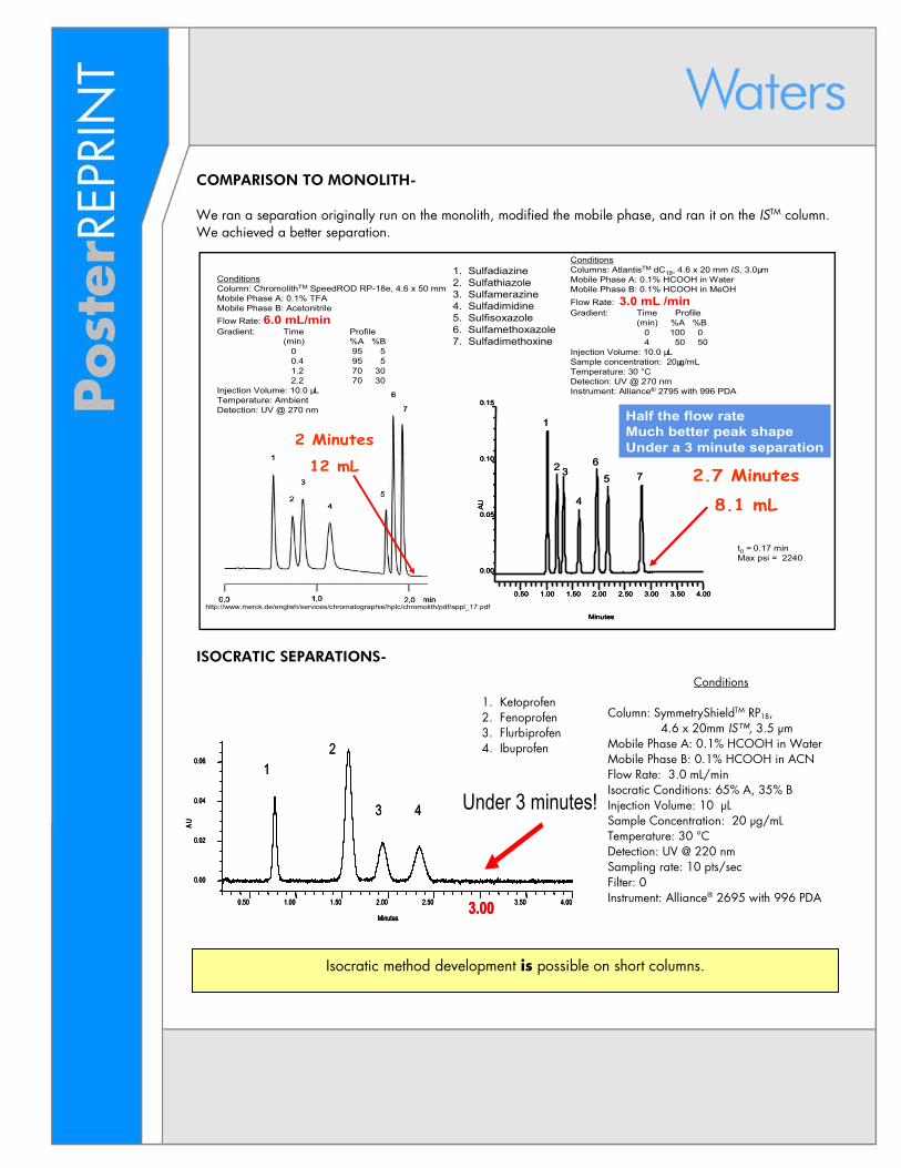
ISOCRATIC SEPARATIONS-

ConditionsColumn: ChromolithTM SpeedROD RP-18e, 4.6 x 50 mmMobile Phase A: 0.1% TFAMobile Phase B: AcetonitrileFlow Rate: 6.0 mL/minGradient: Time Profile

(min) %A %B0 95 50.4 95 51.2 70 302.2 70 30

Injection Volume: 10.0 µLTemperature: AmbientDetection: UV @ 270 nm

1. Sulfadiazine2. Sulfathiazole3. Sulfamerazine4. Sulfadimidine5. Sulfisoxazole6. Sulfamethoxazole7. Sulfadimethoxine

http://www.merck.de/english/services/chromatographie/hplc/chromolith/pdf/appl_17.pdf

ConditionsColumns: AtlantisTM dC18, 4.6 x 20 mm IS, 3.0 µmMobile Phase A: 0.1% HCOOH in WaterMobile Phase B: 0.1% HCOOH in MeOHFlow Rate: 3.0 mL /minGradient: Time Profile

(min) %A %B0 100 0 4 50 50

Injection Volume: 10.0 µLSample concentration: 20 µg/mLTemperature: 30 °CDetection: UV @ 270 nmInstrument: Alliance® 2795 with 996 PDA

t0 = 0.17 minMax psi = 2240

AU

0.00

0.05

0.10

0.15

Minutes

0.50 1.00 1.50 2.00 2.50 3.00 3.50 4.00

4

5

1

2 36

7A

U

0.00

0.05

0.10

0.15

Minutes

0.50 1.00 1.50 2.00 2.50 3.00 3.50 4.00

AU

0.00

0.05

0.10

0.15

Minutes

0.50 1.00 1.50 2.00 2.50 3.00 3.50 4.00

4

5

1

2 36

7

Half the flow rate Much better peak shapeUnder a 3 minute separation

2.7 Minutes

8.1 mL

2 Minutes

12 mL

12

43

AU

0.00

0.02

0.04

0.06

Minutes

0.50 1.00 1.50 2.00 2.50 3.00 3.50 4.00

12

43

AU

0.00

0.02

0.04

0.06

Minutes

0.50 1.00 1.50 2.00 2.50 3.00 3.50 4.00

AU

0.00

0.02

0.04

0.06

Minutes

0.50 1.00 1.50 2.00 2.50 3.00 3.50 4.00

Under 3 minutes!

Isocratic method development is possible on short columns.

Conditions

Column: SymmetryShieldTM RP18, 4.6 x 20mm IS™, 3.5 µm Mobile Phase A: 0.1% HCOOH in Water Mobile Phase B: 0.1% HCOOH in ACN Flow Rate: 3.0 mL/min Isocratic Conditions: 65% A, 35% B Injection Volume: 10 µL Sample Concentration: 20 µg/mL Temperature: 30 °C Detection: UV @ 220 nm Sampling rate: 10 pts/sec Filter: 0 Instrument: Alliance® 2695 with 996 PDA

1. Ketoprofen 2. Fenoprofen 3. Flurbiprofen 4. Ibuprofen

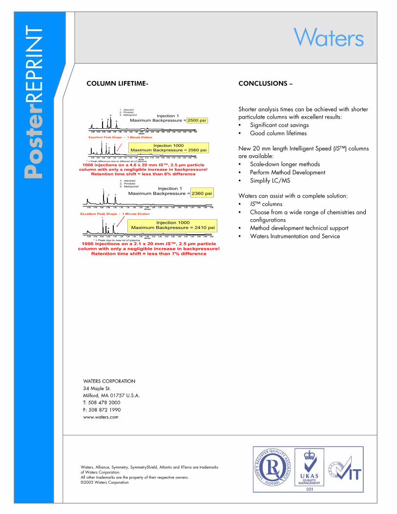
COLUMN LIFETIME-

CONCLUSIONS – Shorter analysis times can be achieved with shorter particulate columns with excellent results: • Significant cost savings • Good column lifetimes New 20 mm length Intelligent Speed (IS™) columns are available: • Scale-down longer methods • Perform Method Development • Simplify LC/MS Waters can assist with a complete solution: • IS™ columns • Choose from a wide range of chemistries and

configurations • Method development technical support • Waters Instrumentation and Service

Waters, Alliance, Symmetry, SymmetryShield, Atlantis and XTerra are trademarks of Waters Corporation. All other trademarks are the property of their respective owners. ©2003 Waters Corporation

Injection 1Maximum Backpressure = 2500 psi

Injection 1000Maximum Backpressure = 2560 psi

1000 injections on a 4.6 x 20 mm IS™, 2.5 µm particlecolumn with only a negligible increase in backpressure!

Retention time shift = less than 6% difference

Minutes0.20 0.40 0.60 0.80 1.00 1.20 1.40 1.60 1.80 2.00 2.20 2.40 2.60 2.80 3.00 3.20 3.40 3.60 3.80 4.00

1 23

Minutes0.20 0.40 0.60 0.80 1.00 1.20 1.40 1.60 1.80 2.00 2.20 2.40 2.60 2.80 3.00 3.20 3.40 3.60 3.80 4.00

Minutes0.20 0.40 0.60 0.80 1.00 1.20 1.40 1.60 1.80 2.00 2.20 2.40 2.60 2.80 3.00 3.20 3.40 3.60 3.80 4.00

1 23

Minutes0.20 0.40 0.60 0.80 1.00 1.20 1.40 1.60 1.80 2.00 2.20 2.40 2.60 2.80 3.00 3.20 3.40 3.60 3.80 4.00

Minutes0.20 0.40 0.60 0.80 1.00 1.20 1.40 1.60 1.80 2.00 2.20 2.40 2.60 2.80 3.00 3.20 3.40 3.60 3.80 4.00

12 3

Excellent Peak Shape – 1 Minute Elution

1. Atenolol2. Pindolol3. Metoprolol

* = Peak difference due to different lot of plasma

*

*

Minutes0.20 0.40 0.60 0.80 1.00 1.20 1.40 1.60 1.80 2.00 2.20 2.40 2.60 2.80 3.00 3.20 3.40 3.60 3.80 4.00

Minutes0.20 0.40 0.60 0.80 1.00 1.20 1.40 1.60 1.80 2.00 2.20 2.40 2.60 2.80 3.00 3.20 3.40 3.60 3.80 4.00

1

2 3

Injection 1Maximum Backpressure = 2360 psi

Minutes0.20 0.40 0.60 0.80 1.00 1.20 1.40 1.60 1.80 2.00 2.20 2.40 2.60 2.80 3.00 3.20 3.40 3.60 3.80 4.00

Minutes0.20 0.40 0.60 0.80 1.00 1.20 1.40 1.60 1.80 2.00 2.20 2.40 2.60 2.80 3.00 3.20 3.40 3.60 3.80 4.00

1

2 3 Injection 1000Maximum Backpressure = 2410 psi

1000 injections on a 2.1 x 20 mm IS™, 2.5 µm particle column with only a negligible increase in backpressure!

Retention time shift = less than 7% difference

Excellent Peak Shape - 1 Minute Elution

*

* = Peak due to new lot of plasma

1. Atenolol2. Pindolol3. Metoprolol