Embed Size (px)
Citation preview
Maximum Entropy andMaximum Entropy andMaximum Entropy andMaximum Entropy andMaximum Entropy andSpecies Distribution ModelingSpecies Distribution ModelingSpecies Distribution ModelingSpecies Distribution ModelingSpecies Distribution Modeling
Rob Schapire
Steven PhillipsMiro Dudık
Also including work by or with: Rob Anderson, Jane Elith, Catherine Gra-
ham, Chris Raxworthy, NCEAS Working Group, ...

The Problem: Species Habitat ModelingThe Problem: Species Habitat ModelingThe Problem: Species Habitat ModelingThe Problem: Species Habitat ModelingThe Problem: Species Habitat Modeling
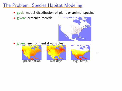
• goal: model distribution of plant or animal species

The Problem: Species Habitat ModelingThe Problem: Species Habitat ModelingThe Problem: Species Habitat ModelingThe Problem: Species Habitat ModelingThe Problem: Species Habitat Modeling
• goal: model distribution of plant or animal species
• given: presence records
The Problem: Species Habitat ModelingThe Problem: Species Habitat ModelingThe Problem: Species Habitat ModelingThe Problem: Species Habitat ModelingThe Problem: Species Habitat Modeling
• goal: model distribution of plant or animal species
• given: presence records
• given: environmental variables
precipitation wet days avg. temp.
· · ·
The Problem: Species Habitat ModelingThe Problem: Species Habitat ModelingThe Problem: Species Habitat ModelingThe Problem: Species Habitat ModelingThe Problem: Species Habitat Modeling
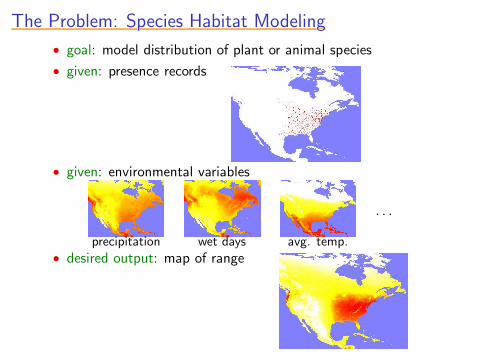
• goal: model distribution of plant or animal species
• given: presence records
• given: environmental variables
precipitation wet days avg. temp.
· · ·
• desired output: map of range

Biological ImportanceBiological ImportanceBiological ImportanceBiological ImportanceBiological Importance
• fundamental question: what are survival requirements (niche)of given species?
• core problem for conservation of species
• first step for many applications:
• reserve design• impact of climate change• discovery of new species• clarification of taxonomic boundaries

A Challenge for Machine LearningA Challenge for Machine LearningA Challenge for Machine LearningA Challenge for Machine LearningA Challenge for Machine Learning
• no negative examples
• very limited data• often, only 20-100 presence records• usually, not systematically collected• may be museum records years or decades old
• sample bias• (toward most accessible locations)

Our ApproachOur ApproachOur ApproachOur ApproachOur Approach
• assume presence records come from probability distribution π
• try to estimate π
• apply maximum entropy approach
Maxent ApproachMaxent ApproachMaxent ApproachMaxent ApproachMaxent Approach
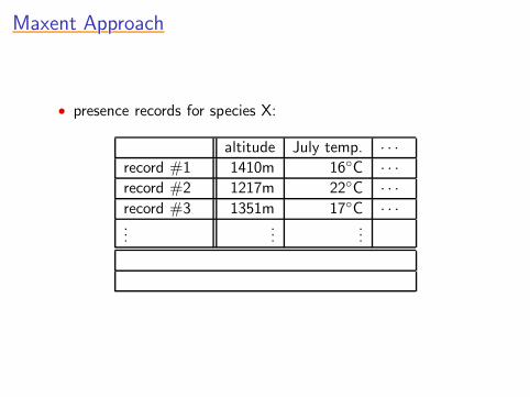
• presence records for species X:
altitude July temp. · · ·
record #1 1410m 16◦C · · ·
record #2 1217m 22◦C · · ·
record #3 1351m 17◦C · · ·...
......
Maxent ApproachMaxent ApproachMaxent ApproachMaxent ApproachMaxent Approach
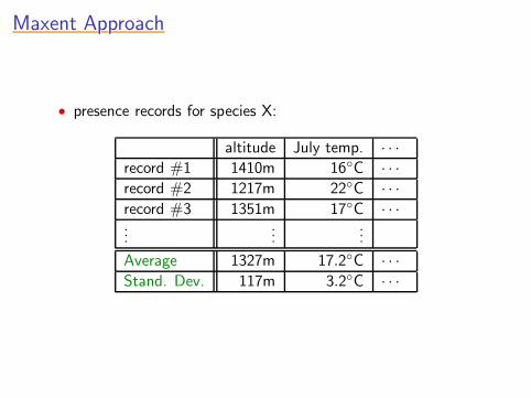
• presence records for species X:
altitude July temp. · · ·
record #1 1410m 16◦C · · ·
record #2 1217m 22◦C · · ·
record #3 1351m 17◦C · · ·...
......
Average 1327m 17.2◦C · · ·
Stand. Dev. 117m 3.2◦C · · ·
Maxent Approach (cont.)Maxent Approach (cont.)Maxent Approach (cont.)Maxent Approach (cont.)Maxent Approach (cont.)
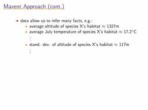
• data allow us to infer many facts, e.g.:• average altitude of species X’s habitat ≈ 1327m• average July temperature of species X’s habitat ≈ 17.2◦C
...• stand. dev. of altitude of species X’s habitat ≈ 117m
...
Maxent Approach (cont.)Maxent Approach (cont.)Maxent Approach (cont.)Maxent Approach (cont.)Maxent Approach (cont.)
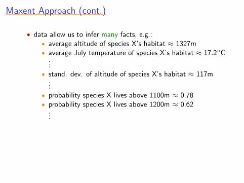
• data allow us to infer many facts, e.g.:• average altitude of species X’s habitat ≈ 1327m• average July temperature of species X’s habitat ≈ 17.2◦C
...• stand. dev. of altitude of species X’s habitat ≈ 117m
...• probability species X lives above 1100m ≈ 0.78• probability species X lives above 1200m ≈ 0.62
...
Maxent Approach (cont.)Maxent Approach (cont.)Maxent Approach (cont.)Maxent Approach (cont.)Maxent Approach (cont.)
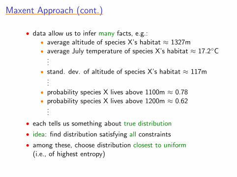
• data allow us to infer many facts, e.g.:• average altitude of species X’s habitat ≈ 1327m• average July temperature of species X’s habitat ≈ 17.2◦C
...• stand. dev. of altitude of species X’s habitat ≈ 117m
...• probability species X lives above 1100m ≈ 0.78• probability species X lives above 1200m ≈ 0.62
...
• each tells us something about true distribution
• idea: find distribution satisfying all constraints
• among these, choose distribution closest to uniform(i.e., of highest entropy)
This TalkThis TalkThis TalkThis TalkThis Talk
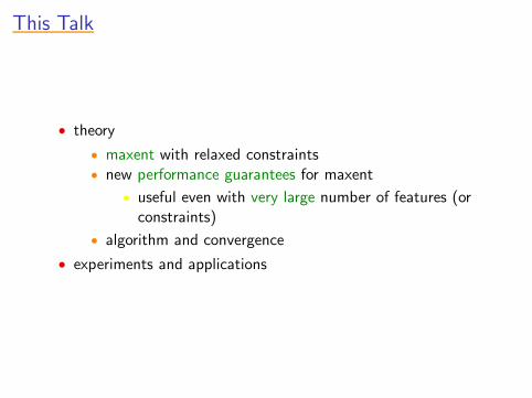
• theory
• maxent with relaxed constraints• new performance guarantees for maxent
• useful even with very large number of features (orconstraints)
• algorithm and convergence
• experiments and applications

The Abstract FrameworkThe Abstract FrameworkThe Abstract FrameworkThe Abstract FrameworkThe Abstract Framework
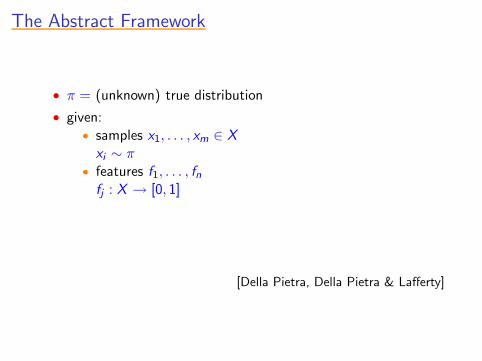
• π = (unknown) true distribution
[Della Pietra, Della Pietra & Lafferty]
The Abstract FrameworkThe Abstract FrameworkThe Abstract FrameworkThe Abstract FrameworkThe Abstract Framework
• π = (unknown) true distribution
• given:• samples x1, . . . , xm ∈ X
xi ∼ π• features f1, . . . , fn
fj : X → [0, 1]
[Della Pietra, Della Pietra & Lafferty]
The Abstract FrameworkThe Abstract FrameworkThe Abstract FrameworkThe Abstract FrameworkThe Abstract Framework
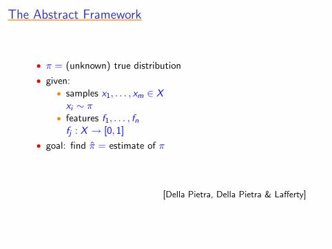
• π = (unknown) true distribution
• given:• samples x1, . . . , xm ∈ X
xi ∼ π• features f1, . . . , fn
fj : X → [0, 1]
• goal: find π = estimate of π
[Della Pietra, Della Pietra & Lafferty]
Maxent and Habitat ModelingMaxent and Habitat ModelingMaxent and Habitat ModelingMaxent and Habitat ModelingMaxent and Habitat Modeling
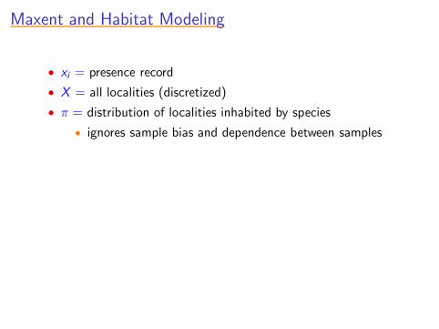
• xi = presence record
• X = all localities (discretized)
• π = distribution of localities inhabited by species
• ignores sample bias and dependence between samples
Maxent and Habitat ModelingMaxent and Habitat ModelingMaxent and Habitat ModelingMaxent and Habitat ModelingMaxent and Habitat Modeling
• xi = presence record
• X = all localities (discretized)
• π = distribution of localities inhabited by species
• ignores sample bias and dependence between samples
• features: use raw environmental variables vk
• linear: fj = vk
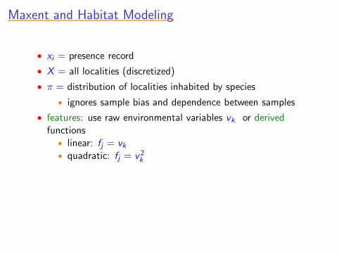
Maxent and Habitat ModelingMaxent and Habitat ModelingMaxent and Habitat ModelingMaxent and Habitat ModelingMaxent and Habitat Modeling
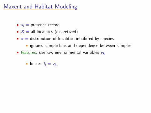
• xi = presence record
• X = all localities (discretized)
• π = distribution of localities inhabited by species
• ignores sample bias and dependence between samples
• features: use raw environmental variables vk or derivedfunctions
• linear: fj = vk
• quadratic: fj = v2
k
Maxent and Habitat ModelingMaxent and Habitat ModelingMaxent and Habitat ModelingMaxent and Habitat ModelingMaxent and Habitat Modeling
• xi = presence record
• X = all localities (discretized)
• π = distribution of localities inhabited by species
• ignores sample bias and dependence between samples
• features: use raw environmental variables vk or derivedfunctions
• linear: fj = vk
• quadratic: fj = v2
k
• product: fj = vkv`
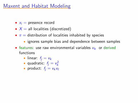
• threshold: fj =
{1 if vk ≥ a
0 else
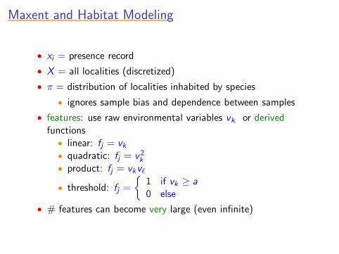
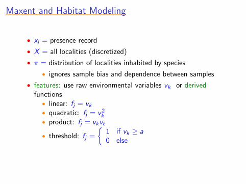
• # features can become very large (even infinite)
A Bit More NotationA Bit More NotationA Bit More NotationA Bit More NotationA Bit More Notation
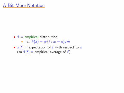
• π = empirical distribution• i.e., π(x) = #{i : xi = x}/m
• π[f ] = expectation of f with respect to π(so π[f ] = empirical average of f )

MaxentMaxentMaxentMaxentMaxent
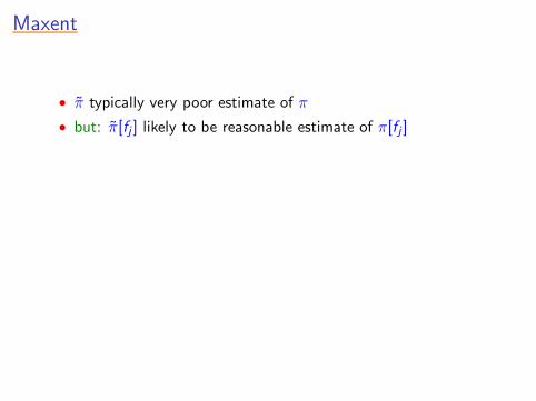
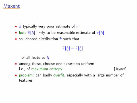
• π typically very poor estimate of π
MaxentMaxentMaxentMaxentMaxent
• π typically very poor estimate of π
• but: π[fj ] likely to be reasonable estimate of π[fj ]
MaxentMaxentMaxentMaxentMaxent
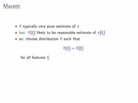
• π typically very poor estimate of π
• but: π[fj ] likely to be reasonable estimate of π[fj ]
• so: choose distribution π such that
π[fj ] = π[fj ]
for all features fj
MaxentMaxentMaxentMaxentMaxent
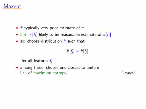
• π typically very poor estimate of π
• but: π[fj ] likely to be reasonable estimate of π[fj ]
• so: choose distribution π such that
π[fj ] = π[fj ]
for all features fj
• among these, choose one closest to uniform,i.e., of maximum entropy [Jaynes]
MaxentMaxentMaxentMaxentMaxent
• π typically very poor estimate of π
• but: π[fj ] likely to be reasonable estimate of π[fj ]
• so: choose distribution π such that
π[fj ] = π[fj ]
for all features fj
• among these, choose one closest to uniform,i.e., of maximum entropy [Jaynes]
• problem: can badly overfit, especially with a large number offeatures
A More Relaxed VersionA More Relaxed VersionA More Relaxed VersionA More Relaxed VersionA More Relaxed Version
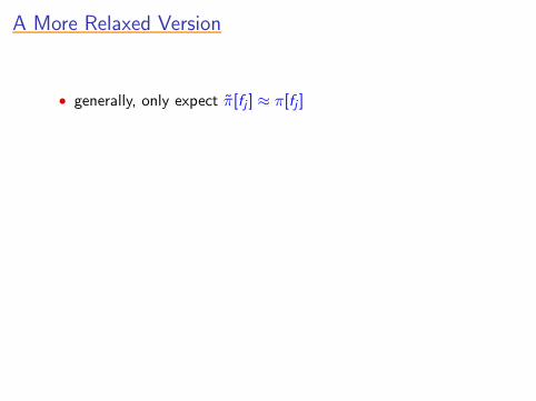
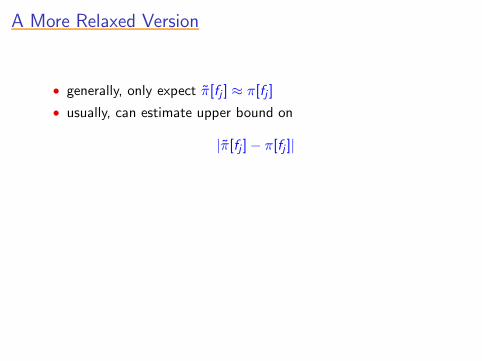
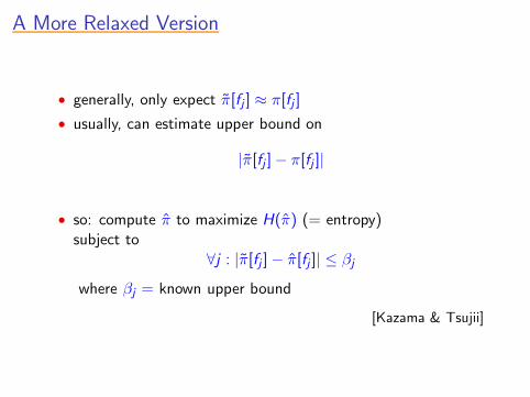
• generally, only expect π[fj ] ≈ π[fj ]
A More Relaxed VersionA More Relaxed VersionA More Relaxed VersionA More Relaxed VersionA More Relaxed Version
• generally, only expect π[fj ] ≈ π[fj ]
• usually, can estimate upper bound on
|π[fj ] − π[fj ]|
A More Relaxed VersionA More Relaxed VersionA More Relaxed VersionA More Relaxed VersionA More Relaxed Version
• generally, only expect π[fj ] ≈ π[fj ]
• usually, can estimate upper bound on
|π[fj ] − π[fj ]|
• so: compute π to maximize H(π) (= entropy)subject to
∀j : |π[fj ] − π[fj ]| ≤ βj
where βj = known upper bound
[Kazama & Tsujii]
DualityDualityDualityDualityDuality
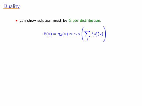
• can show solution must be Gibbs distribution:
π(x) = qλ(x) ∝ exp
∑
j
λj fj(x)

DualityDualityDualityDualityDuality
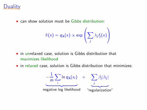
• can show solution must be Gibbs distribution:
π(x) = qλ(x) ∝ exp
∑
j
λj fj(x)
• in unrelaxed case, solution is Gibbs distribution thatmaximizes likelihood, i.e., minimizes:
−1
m
∑
i
ln qλ(xi )
︸ ︷︷ ︸
negative log likelihood
DualityDualityDualityDualityDuality
• can show solution must be Gibbs distribution:
π(x) = qλ(x) ∝ exp
∑
j
λj fj(x)
• in unrelaxed case, solution is Gibbs distribution thatmaximizes likelihood
• in relaxed case, solution is Gibbs distribution that minimizes:
−1
m
∑
i
ln qλ(xi )
︸ ︷︷ ︸
negative log likelihood
+∑
j
βj |λj |
︸ ︷︷ ︸
“regularization”
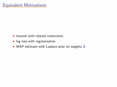
Equivalent MotivationsEquivalent MotivationsEquivalent MotivationsEquivalent MotivationsEquivalent Motivations
• maxent with relaxed constraints
• log loss with regularization
• MAP estimate with Laplace prior on weights λ

How Good Is Maxent Estimate?How Good Is Maxent Estimate?How Good Is Maxent Estimate?How Good Is Maxent Estimate?How Good Is Maxent Estimate?
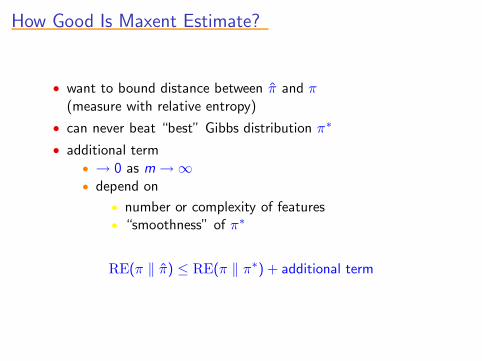
• want to bound distance between π and π(measure with relative entropy)
RE(π ‖ π) ≤
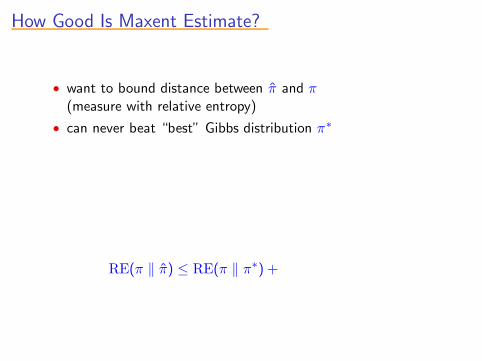
How Good Is Maxent Estimate?How Good Is Maxent Estimate?How Good Is Maxent Estimate?How Good Is Maxent Estimate?How Good Is Maxent Estimate?
• want to bound distance between π and π(measure with relative entropy)
• can never beat “best” Gibbs distribution π∗
RE(π ‖ π) ≤ RE(π ‖ π∗) +
How Good Is Maxent Estimate?How Good Is Maxent Estimate?How Good Is Maxent Estimate?How Good Is Maxent Estimate?How Good Is Maxent Estimate?
• want to bound distance between π and π(measure with relative entropy)
• can never beat “best” Gibbs distribution π∗
• additional term• → 0 as m → ∞• depend on
• number or complexity of features• “smoothness” of π∗
RE(π ‖ π) ≤ RE(π ‖ π∗) + additional term
Bounds for Finite Feature ClassesBounds for Finite Feature ClassesBounds for Finite Feature ClassesBounds for Finite Feature ClassesBounds for Finite Feature Classes
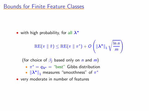
• with high probability, for all λ∗
RE(π ‖ π) ≤ RE(π ‖ π∗) + O
(
‖λ∗‖
1
√
lnn
m
)
(for choice of βj based only on n and m)
• π∗ = qλ∗ = “best” Gibbs distribution• ‖λ∗‖
1measures “smoothness” of π∗
• very moderate in number of features
Bounds for Infinite Binary Feature ClassesBounds for Infinite Binary Feature ClassesBounds for Infinite Binary Feature ClassesBounds for Infinite Binary Feature ClassesBounds for Infinite Binary Feature Classes
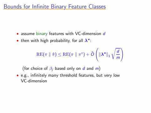
• assume binary features with VC-dimension d
• then with high probability, for all λ∗:
RE(π ‖ π) ≤ RE(π ‖ π∗) + O
(
‖λ∗‖1
√
d
m
)
(for choice of βj based only on d and m)
• e.g., infinitely many threshold features, but very lowVC-dimension
Main TheoremMain TheoremMain TheoremMain TheoremMain Theorem
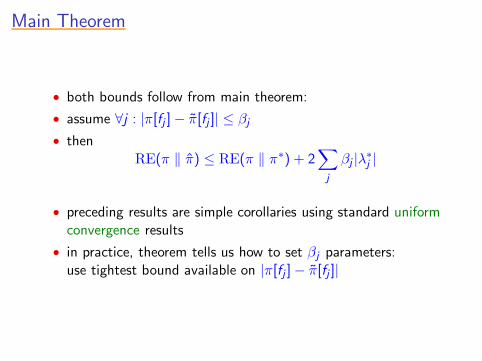
• both bounds follow from main theorem:
• assume ∀j : |π[fj ] − π[fj ]| ≤ βj
• thenRE(π ‖ π) ≤ RE(π ‖ π∗) + 2
∑
j
βj |λ∗
j |
• preceding results are simple corollaries using standard uniformconvergence results
• in practice, theorem tells us how to set βj parameters:use tightest bound available on |π[fj ] − π[fj ]|
Finding an AlgorithmFinding an AlgorithmFinding an AlgorithmFinding an AlgorithmFinding an Algorithm
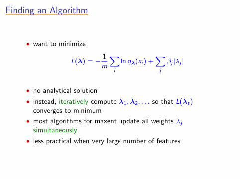
• want to minimize
L(λ) = −1
m
∑
i
ln qλ(xi) +∑
j
βj |λj |
• no analytical solution
• instead, iteratively compute λ1,λ2, . . . so that L(λt)converges to minimum
• most algorithms for maxent update all weights λj
simultaneously
• less practical when very large number of features
Sequential-update AlgorithmSequential-update AlgorithmSequential-update AlgorithmSequential-update AlgorithmSequential-update Algorithm
• instead update just one weight at a time
• leads to sparser solution
• sometimes can search for best weight to update very efficiently
• analogous to boosting• weak learner acts as oracle for choosing function (weak
classifier) from large space
• can prove convergence to minimum of L
Experiments and ApplicationsExperiments and ApplicationsExperiments and ApplicationsExperiments and ApplicationsExperiments and Applications
• broad comparison of algorithms• improvements by handling sample bias
• case study
• discovering new species
• clarification of taxonomic boundaries
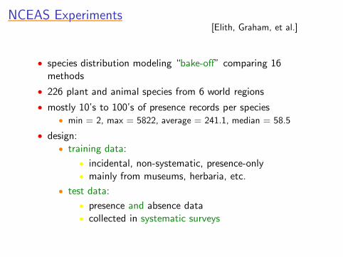
NCEAS ExperimentsNCEAS ExperimentsNCEAS ExperimentsNCEAS ExperimentsNCEAS Experiments[Elith, Graham, et al.]
• species distribution modeling “bake-off” comparing 16methods
• 226 plant and animal species from 6 world regions
• mostly 10’s to 100’s of presence records per species• min = 2, max = 5822, average = 241.1, median = 58.5
• design:• training data:
• incidental, non-systematic, presence-only• mainly from museums, herbaria, etc.
• test data:
• presence and absence data• collected in systematic surveys
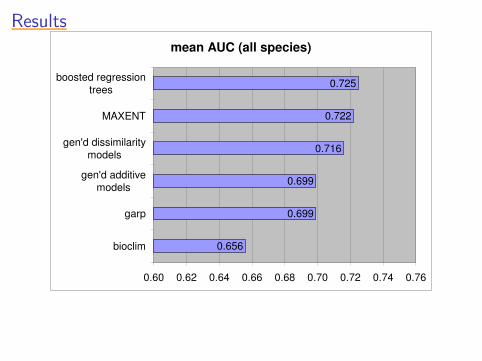
ResultsResultsResultsResultsResults
mean AUC (all species)
0.656
0.699
0.699
0.716
0.722
0.725
0.60 0.62 0.64 0.66 0.68 0.70 0.72 0.74 0.76
bioclim
garp
gen'd additivemodels
gen'd dissimilaritymodels
MAXENT
boosted regressiontrees
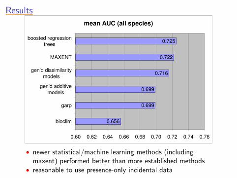
ResultsResultsResultsResultsResults
mean AUC (all species)
0.656
0.699
0.699
0.716
0.722
0.725
0.60 0.62 0.64 0.66 0.68 0.70 0.72 0.74 0.76
bioclim
garp
gen'd additivemodels
gen'd dissimilaritymodels
MAXENT
boosted regressiontrees
• newer statistical/machine learning methods (includingmaxent) performed better than more established methods
• reasonable to use presence-only incidental data
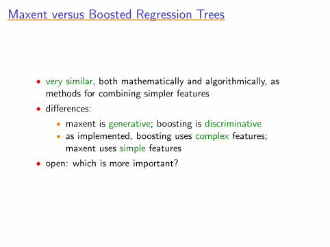
Maxent versus Boosted Regression TreesMaxent versus Boosted Regression TreesMaxent versus Boosted Regression TreesMaxent versus Boosted Regression TreesMaxent versus Boosted Regression Trees
• very similar, both mathematically and algorithmically, asmethods for combining simpler features
• differences:
• maxent is generative; boosting is discriminative• as implemented, boosting uses complex features;
maxent uses simple features
• open: which is more important?
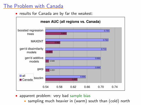
The Problem with CanadaThe Problem with CanadaThe Problem with CanadaThe Problem with CanadaThe Problem with Canada• results for Canada are by far the weakest:
mean AUC (all regions vs. Canada)
0.632
0.560
0.582
0.601
0.656
0.699
0.699
0.722
0.725
0.549
0.551
0.716
0.54 0.58 0.62 0.66 0.70 0.74
bioclim
garp
gen'd additivemodels
gen'd dissimilaritymodels
MAXENT
boosted regressiontrees
allCanada
• apparent problem: very bad sample bias• sampling much heavier in (warm) south than (cold) north
Sample BiasSample BiasSample BiasSample BiasSample Bias
• can modify maxent to handle sample bias
• use sampling distribution (assume known) as “default”distribution (instead of uniform)
• then factor bias out from final model
• problem: where to get sampling distribution

Sample BiasSample BiasSample BiasSample BiasSample Bias
• can modify maxent to handle sample bias
• use sampling distribution (assume known) as “default”distribution (instead of uniform)
• then factor bias out from final model
• problem: where to get sampling distribution
• typically, modeling many species at once
• so, for sampling distribution, use all locations where anyspecies observed
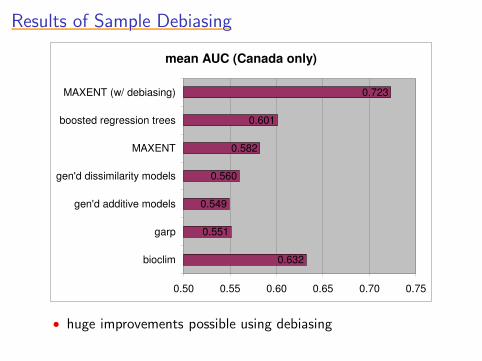
Results of Sample DebiasingResults of Sample DebiasingResults of Sample DebiasingResults of Sample DebiasingResults of Sample Debiasing
mean AUC (Canada only)
0.632
0.551
0.549
0.560
0.582
0.601
0.723
0.50 0.55 0.60 0.65 0.70 0.75
bioclim
garp
gen'd additive models
gen'd dissimilarity models
MAXENT
boosted regression trees
MAXENT (w/ debiasing)
• huge improvements possible using debiasing
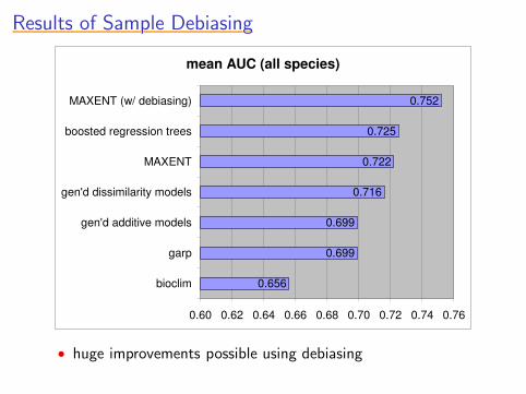
Results of Sample DebiasingResults of Sample DebiasingResults of Sample DebiasingResults of Sample DebiasingResults of Sample Debiasing
mean AUC (all species)
0.656
0.699
0.699
0.716
0.722
0.725
0.752
0.60 0.62 0.64 0.66 0.68 0.70 0.72 0.74 0.76
bioclim
garp
gen'd additive models
gen'd dissimilarity models
MAXENT
boosted regression trees
MAXENT (w/ debiasing)
• huge improvements possible using debiasing
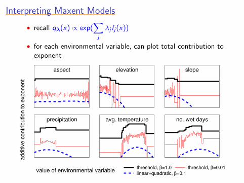
Interpreting Maxent ModelsInterpreting Maxent ModelsInterpreting Maxent ModelsInterpreting Maxent ModelsInterpreting Maxent Models
• recall qλ(x) ∝ exp(∑
j
λj fj(x))
• for each environmental variable, can plot total contribution toexponent
value of environmental variable
addi
tive
cont
ribut
ion
to e
xpon
ent
threshold, β=1.0 threshold, β=0.01linear+quadratic, β=0.1
aspect elevation slope
precipitation avg. temperature no. wet days
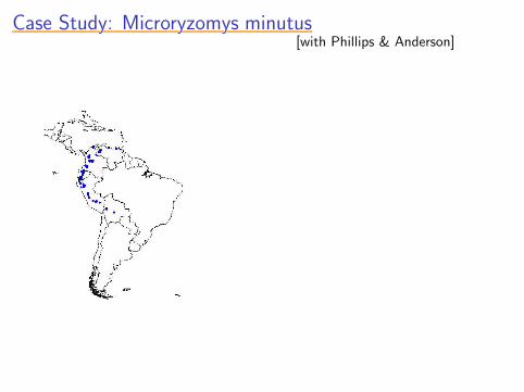
Case Study: Microryzomys minutusCase Study: Microryzomys minutusCase Study: Microryzomys minutusCase Study: Microryzomys minutusCase Study: Microryzomys minutus[with Phillips & Anderson]

Case Study: Microryzomys minutusCase Study: Microryzomys minutusCase Study: Microryzomys minutusCase Study: Microryzomys minutusCase Study: Microryzomys minutus[with Phillips & Anderson]
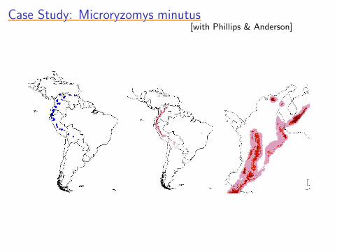
Case Study: Microryzomys minutusCase Study: Microryzomys minutusCase Study: Microryzomys minutusCase Study: Microryzomys minutusCase Study: Microryzomys minutus[with Phillips & Anderson]

Case Study (cont.)Case Study (cont.)Case Study (cont.)Case Study (cont.)Case Study (cont.)
• accurately captures realized range
• did not predict other wet montane forest areas where could
live, but doesn’t• examined predictions of maxent on six of these (chosen
by biologist)• found all had characteristics well outside typical range for
actual presence records
• e.g., four sites had July precipitation ≥ 5 standarddeviations above mean
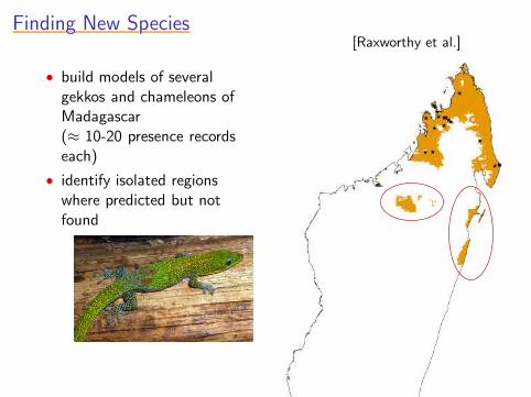
Finding New SpeciesFinding New SpeciesFinding New SpeciesFinding New SpeciesFinding New Species[Raxworthy et al.]
• build models of severalgekkos and chameleons ofMadagascar(≈ 10-20 presence recordseach)
• identify isolated regionswhere predicted but notfound
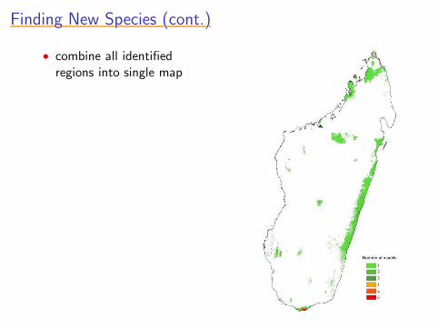
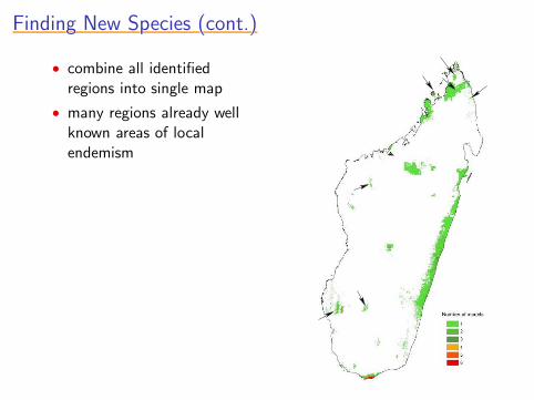
Finding New Species (cont.)Finding New Species (cont.)Finding New Species (cont.)Finding New Species (cont.)Finding New Species (cont.)
• combine all identifiedregions into single map
Finding New Species (cont.)Finding New Species (cont.)Finding New Species (cont.)Finding New Species (cont.)Finding New Species (cont.)
• combine all identifiedregions into single map
• many regions already wellknown areas of localendemism
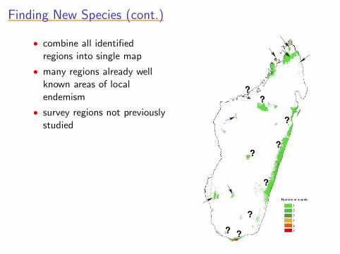
Finding New Species (cont.)Finding New Species (cont.)Finding New Species (cont.)Finding New Species (cont.)Finding New Species (cont.)
• combine all identifiedregions into single map
• many regions already wellknown areas of localendemism
• survey regions not previouslystudied
?
?
??
?
?? ?
?

New SpeciesNew SpeciesNew SpeciesNew SpeciesNew Species
• result: discovery of many new species (possibly 15-30)
Thanks to Chris Raxworthy for all maps and photos!
Clarifying Taxonomic BoundariesClarifying Taxonomic BoundariesClarifying Taxonomic BoundariesClarifying Taxonomic BoundariesClarifying Taxonomic Boundaries[Raxworthy et al.]
• “cryptic species”: classified as single species, but suspectedmixture of ≥ 2 species
• sometimes, maxent model is wildly wrong if trained on allrecords
• but model is much more reasonable if trained on eachsub-population separately
• gives strong evidence actually dealing with multiple species
• can then follow up with morphological or genetic study
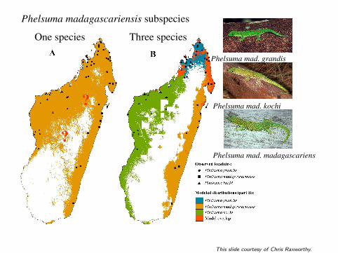
Phelsuma madagascariensis subspecies
Phelsuma mad. grandis
Phelsuma mad. kochi
Phelsuma mad. madagascariensis
One species Three species
?
?
This slide courtesy of Chris Raxworthy.
SummarySummarySummarySummarySummary
• maxent provides clean and effective fit to habitat modelingproblem
• works with positive-only examples
• seems to perform well with limited number of examples
• theoretical guarantees indicate can be used even with a verylarge number of features
• other nice properties:• easy to interpret by human expert• can be extended to handle sample bias
• many biological applications